analysis of a herding model in social economics · analysis of a herding model in social economics...

Analysis of a herding model in social economics

Lara Trussardi1 Ansgar Jungel1 C. Kuhn1

1 Technische Universitat Wien

Taormina - June 13, 2014

www.itn-strike.eu

L. Trussardi, A. Jungel, C. Kuhn (TUW) Analysis of a herding model Taormina - June 13, 2014 1 / 15

www.itn-strike.eu

Index

1 Introduction

2 Mathematical study

3 Bifurcation approach

4 Outlook


Hearding and aim

Herd behavior:a large number of people actingin the same way at the sametime

Stock market:greed in frenzied buying (namedbubbles) and fear in selling(named crash)

Goal

To model information herding in a macroscopic settingwith mathematical analysis


The model

Ω ⊂ Rd : bounded domain, e.g. Ω = (−1, 1)d

x ∈ Ω : multidimensional information variable (political opinion,wealth of individual or company. . . )

u(x , t) : number of people having information x at time t, 0 ≤ u ≤ 1

v(x , t) : influence potential (∇v : influence field), v ∈ R

opinion distribution u

diffusion+source−−−−−−−−−−→←−−−−−−−−−−

drift

influence potential v


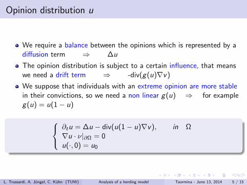
Opinion distribution u

We require a balance between the opinions which is represented by adiffusion term ⇒ ∆u

The opinion distribution is subject to a certain influence, that meanswe need a drift term ⇒ -div(g(u)∇v)

We suppose that individuals with an extreme opinion are more stablein their convictions, so we need a non linear g(u) ⇒ for exampleg(u) = u(1− u)

∂tu = ∆u − div(u(1− u)∇v), in Ω∇u · ν|∂Ω = 0u(·, 0) = u0


Influence potential v

We require averaging i.e. diffusion term with a positive constant⇒ κ∆v , κ > 0

We need a relaxation term that is represented with a linear term in vwith a positive constant ⇒ −αv , α > 0

There is a herding effect that is modelled with a source term⇒ f (u) = u(1− u)

We need a term as a regularization of the equation, enabling us toderive some entropy structure. This is represented with a diffusion inu ⇒ δ∆u for “small“ |δ|

∂tv = δ∆u + κ∆v + u(1− u)− αv , in Ω∇v · ν|∂Ω = 0v(·, 0) = v0

Remark: δ 6= 0 useful for mathematical analysis


The model

Goal: existence of solutions, behaviour for t →∞, stability, bifurcationanalysis

Cross-diffusion model

∂tu = div(∇u − g(u)∇v), in Ω∂tv = δ∆u + κ∆v + f (u)− αv , in Ω(∇u − g(u)∇v) · ν = (δ∇u + κ∇v) · ν = 0, on ∂Ω, t > 0u(·, 0) = u0, v(·, 0) = v0

Main difficulties: the diffusion matrix

(1 −g(u)δ κ

)is not positive

definite

Main idea: entropy method (for δ 6= 0!)


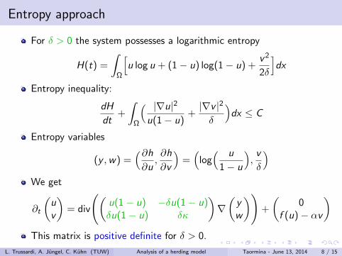
Entropy approach

For δ > 0 the system possesses a logarithmic entropy

H(t) =

∫Ω

[u log u + (1− u) log(1− u) +

v2

2δ

]dx

Entropy inequality:

dH

dt+

∫Ω

( |∇u|2u(1− u)

+|∇v |2

δ

)dx ≤ C

Entropy variables

(y ,w) =(∂h∂u,∂h

∂v

)=(

log( u

1− u

),v

δ

)We get

∂t

(uv

)= div

((u(1− u) −δu(1− u)δu(1− u) δκ

)∇(yw

))+

(0

f (u)− αv

)This matrix is positive definite for δ > 0.


Main result

Global existence theorem

Let Ω ⊂ R2 be a bounded domain with smooth boundary, δ > 0,0 ≤ u0, v0 ∈ L1(Ω) such that H(u0, v0) ≥ 0,⇒ ∃ a weak solution (u, v) with u ≥ 0 in Ω× (0,∞) to

∂tu = div(∇u − u(1− u)∇v)∂tv = δ∆u + κ∆v + u(1− u)− αv

Idea of the proof:

1 approximate elliptic problem: for τ > 0 time discretisation andaddition of the term ε∆2y + εw

2 Leray-Schauder fixed point theorem

3 estimates from entropy inequality for (τ, ε)→ 0

The existence result can be extended to δ < 0 (not too negative)


Steady state

Goal: study under which condition there is congestion of opiniondiv(∇u∞ − u∞(1− u∞)∇v∞) = 0δ∆u∞ + κ∆v∞ + u∞(1− u∞)− αv∞ = 0

Possible steady states (u∞, v∞):

1 constants (u∞, v∞) =(u, u(1−u)α ) with u ∈ [0, 1]

2 non constant (u∞, v∞) = ( 11+e−φ , φ) with φ = v∞ − c

0 = ∇u∞ − u∞(1− u∞)∇v∞ = ∇(v∞ − log

( u∞1− u∞

))and φ solves ∆φ = F (φ,∇φ)


Long time behaviour

Goal: study the exponential decay of the weak solution to thehomogeneous steady state (u∞, v∞)

Long time behaviour by studying the relative entropy

H(u, v) =

∫Ω

[u log(

u

u∞) + (1− u) log(

1− u

1− u∞)]

+(v − v∞)2

2δdx

Conclusion:

positive δ: decay to the constant steady state for t → 0

|u(t)− u∞|2L2(Ω) → 0, |v(t)− v∞|2L2(Ω) → 0,

negative δ: decay to the constant steady state IF AND ONLY IFδ > −4κ

NO herding occurs if δ > −4κ


Bifurcation approach

Goal: study the existence of non-constant steady states

Choose δ as a bifurcation parameter

We can apply bifurcation theory to show that the solutions maybifurcate from the constant steady state (u∞, v∞)

Idea:

1 linearization of the system around the constant steady state (u∞, v∞)

2 study the eigenvalue problem


Crandall-Rabinowitz theorem

We consider ∆U = F(U, δ), with Neumann boundary condition andhomogeneous steady state (w.l.o.g.) U∞ = 0.The eigenvalue problem is:

∆U − (DUF)(0, δ)U = λU

In our model:

U =

(uv

)F(u, v , δ) =

(∇ · (−∇u + g(u)∇v)

−δ∆u − κ∆v + αv − f (u)

)We need to incorporate the mass constraint:

∫Ω u(x)dx − |Ω|u0

Hypothesis:

the Fredholm index of DUF(0, δ) is zero

the null space N(DUF(0, δ)) 6= 0, in particularN(DUF(0, δ)) = span[U]

DδUF(0, δ∗)(U) /∈ R(DUF(0, δ∗))


Crandall-Rabinowitz theorem

Theorem

Assume the previous hypothesis, then there is a non trivial continuoslydifferentiable curve through (0, δ∗)

(U(s), δ(s))|s ∈ (−σ, σ), (U(0), δ(0)) = (0, δ∗)

such that F(U(s), δ(s)) = 0 for s ∈ (−σ, σ) and all solutions ofF(U, δ) = 0 in a neighborhood of (0, δ∗) belong to this curve. Theintersection (0, δ∗) is called a bifurcation point.

Main problems:

prove that the Frechet derivatives of F is a Fredholm operator withindex zerocheck the transversality condition δ′(0) 6= 0study the derivatives of F

We expect a transcritical bifurcation


Further studies

To study under which conditions this model describes herding

Analysis and numerics for negative δ (kind of bifurcation and in whichdirection)

Modelling of herding using a kinetic approach

Possibly identification of this diffusion model as the mean-field limitof the kinetic equation

Thanks for your attention

www.itn-strike.eu


www.itn-strike.eu

analysis of a herding model in social economics · analysis of a herding model in social economics...

Documents