analysis of a dynamically loaded beam bridge in torsion

i

Analysis of a dynamically loaded beam bridge in torsion

Pia Hannewald

TRITA-BKN. Master Thesis 236, Structural Design and Bridges 2006

ISSN 1103-4297

ISRN KTH/BKN/EX--236--SE

iii

Preface This thesis was carried out at the Division of Structural Design and Bridges at the Department of Civil and Architectural Engineering at the Royal Institute of Technology (KTH). The supervisor has been Professor Håkan Sundquist, who also presented the idea for the work done in this thesis. I would like to thank my supervisor Professor Håkan Sundquist and co-supervisor PhD student Johan Wiberg for making it possible for me to write this thesis and thereby take part in the research project at the Årsta Bridge. Thank You very much for Your help and guidance throughout the work and all the time You invested. Stockholm, May 2006 Pia Hannewald

v

Abstract In this thesis, a simple model was developed to analyse the natural torsional frequencies of a concrete box-girder bridge with a simply symmetric, non-uniform cross-section. The superstructure of the bridge is a slender pre-stressed construction with thin walls. Torsional warping can have a significant influence on the behaviour of this kind of box-girder bridges. Therefore, both St.Venant’s torsional stiffness and warping stiffness were considered in the calculation and the influence of warping on the natural frequencies was examined. Vlasov’s theory for thin-walled beams was assumed applicable and used for the calculation of the frequencies. The influence of the non-coincidence of the shear centre and the centre of gravity, as well as the influence of cross-section deformations, were assumed negligible. The calculation of the natural frequencies was done with the finite difference method of central differences. The differential equation for torsion was expressed by finite difference formulations and applied for a single bridge span with boundary conditions determined mainly by the character of the supports. Thereby, matrices representing the span’s torsional stiffness were derived. The eigenvalues and –vectors of these matrices, i.e. the bridge span’s natural frequencies and mode shapes, were calculated with the MATLAB® software. Furthermore, an attempt was made to take the behaviour of the piers into account and thereby develop a model to calculate the frequencies of the whole bridge. The calculated frequencies were compared with frequencies derived from the analysis of in-situ measurements as the bridge is equipped with accelerometers and other instruments for long term monitoring. Accelerometer signals from one main span during train passage were used to calculate the natural frequencies.

vii

Zusammenfassung In dieser Arbeit wurde ein einfaches Model für die Berechnung der Torsionseigen-frequenzen einer Hohlkastenbrücke aus Beton mit einfachsymmetrischem, veränderlichem Querschnitt entwickelt. Der Brückenoberbau ist eine schlanke, dünnwandige Spannbeton Konstruktion. Wölbkraft-torsion kann auf das Torsionsverhalten solcher Brücken einen großen Einfluss haben, weshalb bei der Berechnung der Eigenfrequenzen sowohl die St. Venant’sche Torsions-steifigkeit als auch die Wölbsteifigkeit berücksichtigt wurde. Der Einfluss der Wölbsteifig-keit auf die Torsionseigenfrequenzen dieser Brücke wurde dabei untersucht. Die Berechnungen der Torsionseigenfrequenzen basieren auf Wlassows Theorie für dünn-wandige elastische Stäbe, deren Gültigkeit für diesen Querschnitt vorausgesetzt wurde. Des Weiteren wurde die ungekoppelte Differentialgleichung der Torsion verwendet unter der Vorraussetzung, dass es nur einen geringen Einfluss auf die Eigenfrequenzen hat, dass der Schubmittelpunkt nicht gleich dem Schwerpunkt ist. Eventuelle Querschnitts-verformungen wurden ebenfalls nicht berücksichtigt. Für die Berechnung wurde die Finite Differenzen Methode mit zentralen Differenzen verwendet. Dazu wurde die Differentialgleichung der Torsion mit Hilfe von zentralen Differenzen formuliert und auf die Geometrie des Brückenträgers unter Berücksichtigung der durch die Lagerung vorgegebenen Randbedingungen angewendet. Die Eigenwerte und –vektoren der mit dieser Methode erhaltenen Torsionssteifigkeitsmatrix, d.h. die Eigen-frequenzen und –formen des Brückenträgers, wurden mit der Computersoftware MATLAB® berechnet. Es wurde ausserdem versucht, nicht nur die Frequenzen eines einzelnen Feldes zu berechnen, sondern auch die Schwingungen der Brückenpfeiler zu erfassen und somit ein Model für die Berechnung der Frequenzen der gesamten Brücke zu entwickeln. Die berechneten Frequenzen wurden mit gemessenen Frequenzen verglichen. Diese Frequenzen wurden durch die Analyse von in-situ Messungen während Zugüberfahrten gewonnen. Die Brücke ist unter anderem mit Beschleunigungsmessern instrumentiert, um Langzeitmessungen durchzuführen.

ix

Contents PREFACE ............................................................................................................... iii

ABSTRACT.............................................................................................................. v

ZUSAMMENFASSUNG......................................................................................... vii

1 INTRODUCTION............................................................................................... 1

1.1 Introduction .......................................................................................................................................... 1

1.2 Bridge Information .............................................................................................................................. 2

1.3 Aims of the Study ................................................................................................................................. 2

1.4 Thesis Layout........................................................................................................................................ 3

2 LITERATURE STUDY ...................................................................................... 5

2.1 Introduction .......................................................................................................................................... 5

2.2 Torsion................................................................................................................................................... 5

2.3 Concrete Box-Girders under Torsion................................................................................................ 5

2.4 Influence of Warping on Vibrations .................................................................................................. 6

2.5 Finite Difference Method .................................................................................................................... 7

3 THE FINITE DIFFERENCE METHOD FOR TORSIONAL PROBLEMS......... 9

3.1 Introduction .......................................................................................................................................... 9

3.2 Derivations with Finite Differences.................................................................................................... 9

3.3 Error Terms........................................................................................................................................ 11

3.4 Differential Equation for Torsion .................................................................................................... 11

3.5 Equation Matrices.............................................................................................................................. 13 3.5.1 Matrices for Single Span Model ..................................................................................................... 14 3.5.2 Matrices for Multi Span Model....................................................................................................... 16

3.6 Convergence of Results...................................................................................................................... 20

4 MEASUREMENTS AND SIGNAL ANALYSIS............................................... 23

4.1 Introduction ........................................................................................................................................ 23

4.2 Instrumentation.................................................................................................................................. 24

x

4.3 Fourier Series and the Fast Fourier Transform..............................................................................26

4.4 Time and Frequency Domain ............................................................................................................27

4.5 Windowing...........................................................................................................................................28

4.6 Filtering................................................................................................................................................29

5 RESULTS........................................................................................................31

5.1 Bridge Properties ................................................................................................................................31

5.2 Natural Torsional Frequencies from Single Span Bridge Model..................................................34

5.3 Natural Torsional Frequencies from Multi Span Bridge Model...................................................37

5.4 Natural Torsional Frequencies from Measurements......................................................................39

5.5 Comparison..........................................................................................................................................40

6 DISCUSSION AND CONCLUSION................................................................42

LITERATURE.........................................................................................................44

APPENDIX A..........................................................................................................46

APPENDIX B..........................................................................................................48

APPENDIX C..........................................................................................................50

CHAPTER 1 INTRODUCTION

1

1 Introduction

1.1 Introduction In this thesis, the torsional vibration of the New Årsta Railway Bridge was analysed. Natural torsional frequencies were calculated with a finite difference method and compared with measurements. For both the finite difference calculation of the frequencies and the signal analysis the MATLAB® Software was used. The bridge, located south of Stockholm, was completed and inaugurated in the summer of 2005 after a construction time of five years. It is made of pre-stressed concrete and has a very slender superstructure. The superstructure is a non-uniform box-girder with varying height and diaphragms over the piers. In the calculation of the natural frequencies, the contribution of Saint Venant torsional stiffness and warping stiffness were considered. Two bridge spans were instrumented with amongst others accelerometers to monitor the bridge during construction and in service. Accelerometer signals were analysed to determine the bridge’s natural torsional frequencies. Those were compared with the calculated ones to find out whether the finite difference model satisfactorily describes the actual behaviour. An overview of the bridge location and shape is given in Figure 1.1. An existing bridge next to it is indicated, as well as the island Årsta Holmar and the lake Årstaviken crossed by the bridge.

( )

( )( )

( )( )

( )( )( )( )

( )( )( )( )

( )

( ) ( )( )

( )

( )

( )

ÅRSTAHOLMAR

ÅRSTAVIKEN

TANTO

ÅRSTA

( )( )

( )( )( )( )( )( )( )( )( )( )( )

NL P1 P2 P3 P4 P5 P6 P7 P8 P9 P10 SL

( )

P5 P6 P7 P8 P9 P10 SLP4P3P2

P1

NL EXISTING BRIDGE

Figure 1.1 Overview of the bridge location; from [21].

INTRODUCTION CHAPTER 1

2

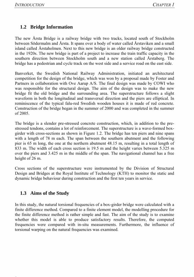
1.2 Bridge Information The new Årsta Bridge is a railway bridge with two tracks, located south of Stockholm between Södermalm and Årsta. It spans over a body of water called Årstaviken and a small island called Årstaholmen. Next to this new bridge is an older railway bridge constructed in the 1920s. The new bridge is part of a project to increase the train traffic capacity in the southern direction between Stockholm south and a new station called Årstaberg. The bridge has a pedestrian and cycle track on the west side and a service road on the east side. Banverket, the Swedish National Railway Administration, initiated an architectural competition for the design of the bridge, which was won by a proposal made by Foster and Partners in collaboration with Ove Aarup A/S. The final design was made by COWI who was responsible for the structural design. The aim of the design was to make the new bridge fit the old bridge and the surrounding area. The superstructure follows a slight waveform in both the longitudinal and transversal direction and the piers are elliptical. In reminiscence of the typical falu-red Swedish wooden houses it is made of red concrete. Construction of the bridge began in the summer of 2000 and was completed in the summer of 2005. The bridge is a slender pre-stressed concrete construction, which, in addition to the pre-stressed tendons, contains a lot of reinforcement. The superstructure is a wave-formed box-girder with cross-sections as shown in Figure 1.2. The bridge has ten piers and nine spans with a length of 78 m each. The span between the southern abutment and the following pier is 65 m long, the one at the northern abutment 48.15 m, resulting in a total length of 833 m. The width of each cross section is 19.5 m and the height varies between 5.325 m over the piers and 3.425 m in the middle of the span. The navigational channel has a free height of 26 m. Cross sections of the superstructure were instrumented by the Division of Structural Design and Bridges at the Royal Institute of Technology (KTH) to monitor the static and dynamic bridge behaviour during construction and the first ten years in service.

1.3 Aims of the Study In this study, the natural torsional frequencies of a box-girder bridge were calculated with a finite difference method. Compared to a finite element model, the modelling procedure for the finite difference method is rather simple and fast. The aim of the study is to examine whether this model is able to produce satisfactory results. Therefore, the computed frequencies were compared with in-situ measurements. Furthermore, the influence of torsional warping on the natural frequencies was examined.

CHAPTER 1 INTRODUCTION

3

116603670 36703425

116603670 3670

5325

Figure 1.2 Cross-sections of the bridge; from [21]. The upper picture shows the cross

section at midspan, the lower picture the cross-section over the piers.

1.4 Thesis Layout Below, each chapter is presented with a short description to give an overview of the thesis. Chapter 2 contains a literature study and general information about the topics dealt with in this thesis. It includes information about the theory of torsion and the behaviour of concrete box-girder bridges subjected to torsion. Information about warping of concrete box-girders and the influence of warping on the natural torsional frequencies of beams is included as well as information on the application of the finite difference method for similar problems. In chapter 3 methods and formulas used for the calculations are explained. The finite difference method of centred differences is introduced and the formulations for the derivatives up to the fourth order are given. The differential equation for torsion of a beam and its notation using finite difference formulations are presented. The composition of the matrices, which are obtained by applying the finite difference equation for every calculation point and which are needed for the calculation with MATLAB®, is presented as

INTRODUCTION CHAPTER 1

4

well. Furthermore, the convergence of the results of finite difference calculations towards the exact analytical result is examined. Chapter 4 contains a short introduction to signal analysis. Fourier Series, which form the mathematical basis for the analysis, are introduced as well as concepts - windowing and filtering - that can be used in the signal analysis process. Moreover, the instrumentation of the bridge with accelerometers is described and the location of the instrumented cross sections as well as the location of the accelerometers in those sections is presented. Chapter 5 contains the results of the finite difference calculations and the signal analysis. The results of the finite difference calculations with a single span bridge model and with a multi span bridge model are presented. The graphs with the cross section properties used for the calculations are included in this chapter as well. The effect of the warping stiffness on the natural frequencies is examined with the single span model. The chapter also includes frequency spectrums from the signal analysis and the comparison of the frequencies in those signals with those from the finite difference calculations. Chapter 6 contains conclusions from the work done in this thesis.

CHAPTER 2 LITERATURE STUDY

5

2 Literature Study

2.1 Introduction A literature study was conducted to study the theory of torsion and the finite difference method. Therefore, literature covering the following topics was searched:

• Torsion: Differential equation for torsion with regard to St. Venant torsion and warping, explanation of the theory and conditions for its application

• Concrete box-girders under torsion: studies on torsional behaviour of box-girders, application of torsional theory and significance of warping

• Influence of warping on vibrations: Significance of considering warping stiffness for the calculation of natural frequencies

• The finite difference method: Derivation of the finite difference formulations and statements about their accuracy, examples for the use of this method for similar problems

2.2 Torsion The theory of torsion is mainly based on the works done by B. de Saint Venant and V. S. Vlasov. St. Venant’s theory is usually applied when the cross-section is non-deformable out of its plain or those deformations are very small. In other cases the more general theory according to Vlasov [22] needs to be applied. Vlasov derives formulations for thin-walled elastic beams with regard to deformations out of the plain, i.e. warping, based on some assumptions regarding the beams geometry and material properties. To develop thin-walled behaviour, the beams length should be ten times greater than the width, and the width ten times greater than the wall thicknesses. Shear deformations are neglected in this theory and the twist is assumed to be small, so that the deformations can be linearised. The material behaviour is assumed linear-elastic and the shear stresses constant over the wall thickness. Based on these assumptions a system of four differential equations, representing four equilibrium conditions, is derived by using geometrical proportions and equilibrium conditions. The system of equations is derived for a general case, where shear centre and centre of gravity need not be the same. If they are on the same axis, this system resolves into four independent equations, one for axial loading, two for bending and one for torsion. In many cases, those four equations are independent of each other, or the interaction is assumed negligible. This was also assumed in this study and the uncoupled differential equation for torsion was applied.

2.3 Concrete Box-Girders under Torsion Box-girders provide a very efficient way of building bridges with low weight and high torsional stiffness. The closed cell of a box-girder can take up and distribute the stresses

LITERATURE STUDY CHAPTER 2

6

resulting from eccentric loading. To spare weight, even concrete box-girder bridges have thin walls compared to the outer dimensions of the cross-section. Nevertheless, compared to a girder made of steel, concrete box-girders do not evidently appear to be thin-walled beams. This, and the fact that closed cells do not warp as much as open sections, often leads to the assumption that warping deformations are negligible and torsion can be treated according to St. Venant’s theory. The application of Vlasov’s theory requires not only thin walls but also linear-elastic material behaviour, which is only approximately fulfilled by concrete for rather low stresses. For these reasons, literature about the behaviour of concrete beams and bridges under torsion was searched. Maisel et al. [9] conducted studies on concrete box-girders to examine amongst others torsional behaviour. Single cell rectangular box-girders with different geometrical proportions and loaded with an eccentric point-load at midspan were examined. The maximum longitudinal stress at the bottom line was increased through warping and distortion of the girder. Waldron et al. [19] conducted studies specifically on the influence of warping on concrete box girders. Rectangular single-cell box-girders with different geometries, i.e. different ratios between wall-thickness and width, were examined in the study. The relation of longitudinal warping stresses to longitudinal bending stresses under an equally distributed eccentric load, instead of a point load as in Maisel’s study, was calculated, for a single span box-girder with diaphragms over the supports. The maximum warping stress at mid-span of a single span bridge was 5 % for the girder geometry analysed in this example, instead of 29 % obtained through a point load. The maximum warping stress in a multi-span bridge was 6 % at midspan, but up to 22 % over the supports in the analysed example. The ratio of warping to bending stresses is influenced by girder geometry and loading and the rather simple geometrical criteria given by Vlasov were found to be insufficient to determine the warping influence. In general it can be stated that, depending on the geometry, torsional warping can have a significant influence on concrete box girder bridges. Mehlhorn, Rützel examined warping torsion in thin-walled reinforced concrete beams with more accurate assumptions for the constitutive equations [12]. Because of the material properties of concrete, the deformation is underestimated when applying Hooke’s Law, especially after the rated strength value of concrete is reached. The stiffness depends on the loading and a low increase of the stress resultants causes a high decrease in stiffness. When a material has a non-linear behaviour, the resistance as well as the shear centre therefore do not only depend on geometry, but also on the stress resultants. In another study by Waldron et al. [20], attention was given to deformation of thin-walled concrete box-girders and the stresses arising through that. Those stresses were significant and higher than the warping stresses in the analysed girders. Depending on the girder geometry, the influence of deformations is therefore considerable.

2.4 Influence of Warping on Vibrations Studies on the effect of warping on the torsional vibrations of thin-walled elastic beams show that the natural frequencies increase when warping stiffness is considered. Li et al. [8] examined the effect of warping on torsional vibration of members with open cross sections and coinciding centre of gravity and shear centre. The effect of considering

CHAPTER 2 LITERATURE STUDY

7

warping in calculating the natural frequencies of beams with constant cross-sections and varying boundary conditions was investigated by setting the frequencies computed with and without regard to warping in relation to each other. The ratio of the jth angular frequencies of a simply supported beam calculated with considering warping stiffness, i.e.

jω , and without considering warping stiffness, i.e. jϖ , is then

1π 2W

2

2

+⎟⎠⎞

⎜⎝⎛=

lj

CC

j

j

ϖω

where CW is the warping stiffness, C the torsional stiffness and l the length of the beam. The influence of warping decreases with increasing l and increases with increasing j, i.e. becomes significant for short beams and high frequencies. The same result was derived in a study by Subrahmanyam, Kaza [18], where pretwisted cantilever beams were examined and the natural torsional frequencies with regard to warping stiffness were always higher than those calculated without it. Warping is especially important for beams with low aspect ratios, i.e. length/ width, and low thickness ratios, i.e. wall thickness/ width, as well as for higher modes. The cross-section geometry and boundary conditions influence the significance of warping as well. In a study by Jun et al. [5] the natural torsional frequencies of axially loaded monosymmetrical Euler-Bernoulli beams with two different cross-section geometries were compared. Warping was significant for all frequencies of a beam with monosymmetrical channel cross-section. In contrast to that, the first three of the five computed frequencies of a beam with semi-circular cross-section were not significantly affected by warping but the next two. When this beam had clamped supports on both ends, all frequencies were influenced by warping as well.

2.5 Finite Difference Method Finite difference formulations for ordinary differential equations can found in manuals for numerical methods with computer programmes [10][15]. Derivatives of a function may be expressed by finite difference formulations of different accuracy. To express the accuracy of a formulation, error terms obtained by Taylor series expansion can be used. Those terms depend on the grid spacing and therefore become smaller with a finer grid. The centred difference approach mainly used in this thesis depends on the squared spacing, but there are also more accurate formulations. To calculate the eigenfrequencies of a beam, its differential equation is expressed by finite difference formulations and the eigenvalues are computed. Petersen [14] gives examples for the use of this method for eigenfrequency calculations of beams with constant cross section. Those calculations are rather simple, but accurate even with regard to elastic supports and only few points for the numerical calculation. A collection of examples for the expression of the differential equations of beams with variable cross-sections and varying boundary conditions is found in [23]. The Årsta Bridge is comparable with the continuous beam in this paper or, if only one span is considered, with a simple beam and the necessary boundary conditions.

LITERATURE STUDY CHAPTER 2

8

A finite difference analysis can be used to calculate the natural frequencies of non-uniform Euler-Bernoulli or cantilever beams with good results, as the following studies show. In a study where the natural frequencies of non-uniform Euler-Bernoulli beams were calculated, Richardson extrapolation was used to improve the results [13]. The relative error increased for higher modes but was in general very small. Another way of improving the results was chosen in another study, where finite difference formulations with better accuracy, i.e. error terms depending on λ4 instead of λ2, with λ being the grid spacing, were used [17]. Nevertheless, the results obtained with lesser accuracy were also satisfactory. It can generally be stated, that the accuracy of the method increases with refined grid spacing, resulting in more points for the numerical calculation, and decreases for higher modes. As a part of a doctoral thesis at KTH, the response of cable-stayed and suspension bridges to vehicles was studied using a finite difference method [6]. Even for this rather complex bridge model, taking into account cables and vehicles, the results were satisfying and considered accurate enough for preliminary studies. However, for a more detailed analysis, taking into account exact cable behaviour, for instance, this method was found to be unsuitable

CHAPTER 3 THE FINITE DIFFERENCE METHOD FOR TORSIONAL PROBLEMS

9

3 The Finite Difference Method for Torsional Problems

3.1 Introduction The finite difference method is based on the numerical approximation for the derivative

)(xf ′ of a function f(x):

λλ

λ

)()(lim)('0

xfxfxf −+=

→ (3.1)

An approximation of the derivative is therefore given by

λλ )()()(' xfxfxf −+

≈ . (3.2)

Equation (3.2) is a so called forward difference approximation. Hereby, the derivative of the function is expressed through the derivative of a secant through the two points f(x) and f(x+λ). If instead of f(x) another value to the left is taken into account, the derivative can be approximated by a centred difference

),(2

)()()(' λλ

λλ fExfxfxf +−−+

= (3.3)

where E(f ,λ) is the error. The centred difference approximates the first derivative more exact than a one sided difference. Using Taylor series expansion the error in this centred difference is dependent on λ², whereas it is dependent on λ in the one sided approach in (3.2). Error terms will be addressed later on.

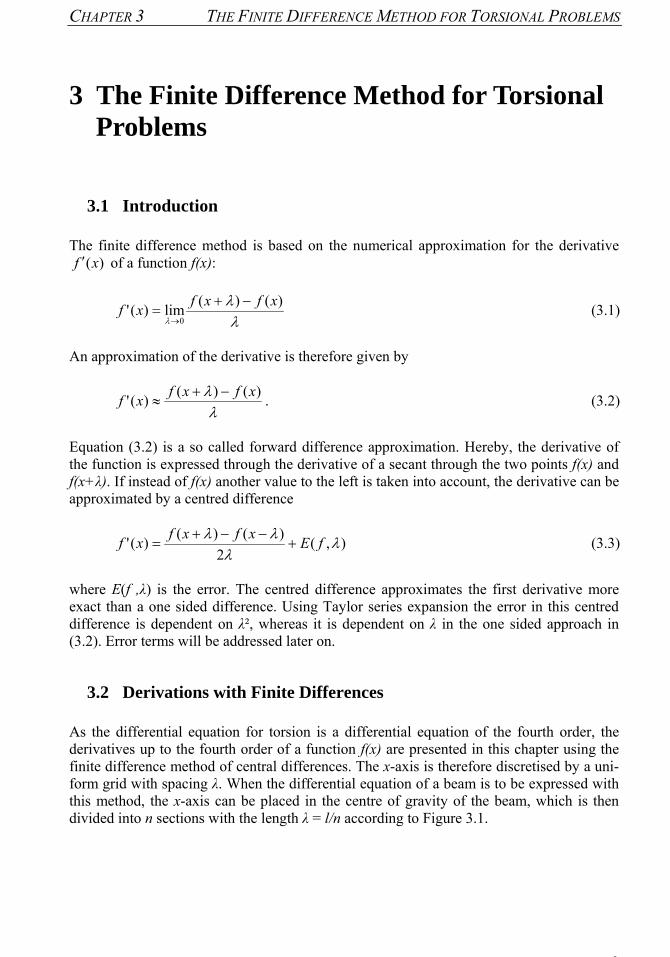
3.2 Derivations with Finite Differences As the differential equation for torsion is a differential equation of the fourth order, the derivatives up to the fourth order of a function f(x) are presented in this chapter using the finite difference method of central differences. The x-axis is therefore discretised by a uni-form grid with spacing λ. When the differential equation of a beam is to be expressed with this method, the x-axis can be placed in the centre of gravity of the beam, which is then divided into n sections with the length λ = l/n according to Figure 3.1.

THE FINITE DIFFERENCE METHOD FOR TORSIONAL PROBLEMS CHAPTER 3

10

Figure 3.1 Beam with n sections.

The derivatives of the function f(x) from the first to the fourth order at a point j on the grid are:

)(21

dd

11 +− +−≈ jj ffxf

λ

)2(²

1²d

²d11 +− +−≈ jjj fff

xf

λ

)22(³2

1³d

³d2112 ++−− +−+−≈ jjjj ffff

xf

λ

)464(1dd

211244

4

++−− +−+−≈ jjjjj fffffx

fλ

(3.4 a-d)

The error terms of the derivatives expressed with the formulas in equations (3.4 a-d) depend on λ². The accuracy of the finite difference expressions can be increased with other formulations. With an error term depending on λ4 the derivatives are:

( )2112 8812

1dd

++−− −+−≈ jjjj ffffxf

λ

( )211222

2

16301612

1dd

++−− −+−+−≈ jjjjj fffffx

fλ

( )32112333

3

81313881

dd

+++−−− −+−+−≈ jjjjjj ffffffx

fλ

( )32112344

4

123956391261

dd

+++−−− −+−+−+−≈ jjjjjjj fffffffx

fλ

(3.5 a-d)

0 1 2 3 …. j-1 j j+1 n-2 n-1 n

λ

l


11

In the following paragraphs, the derivation of the differential equation in finite difference notation and composition of the matrices is presented for equations (3.4 a-d) only. Matrices including the higher order difference equations (3.5 a-d) are obtained the same way.

3.3 Error Terms The central difference formulas given in (3.4a-d) are approximations of the derivatives. Taylor series expansion can be used to approximate the values for f(x+λ) and f(x−λ) and thereby describe the difference between the exact derivative and the numerical approach. The functions f(x+λ) and f(x−λ) expressed by Taylor series expansion are

K+′′′

+′′

+′+=+6

)(2

)()()()(32 λλλλ xfxfxfxfxf

K+′′′

−′′

+′−=−6

)(2

)()()()(32 λλλλ xfxfxfxfxf (3.6)

These terms are subtracted and the Taylor series is truncated at the third derivative. Taylor’s theorem states that there is a value c with |c – x| < λ so that

6)(2)(2)()(

3λλλλ cfxfxfxf′′′

+′=−−+ (3.7)

This equation is solved for ( )xf ′ , which yields

6)(

2)()()(

2λλ

λλ cfxfxfxf′′′

−−−+

=′ (3.8)

The first part of the formula on the right side is the finite difference formula for the first derivative as in equation (3.4a) and the second part is the truncation error. As the truncation error depends on λ² this finite difference formula is called a formula of order O(λ²). The error terms for the difference formulas (3.5 a-d) are derived in a similar way. In numerical calculations, the round-off error, which is depending on the number of decimal places, might also become considerable [10]. However, with the precision of a computer program this should not be a problem, as the number of decimal places is high.

3.4 Differential Equation for Torsion The partial differential equation for torsion for a beam with both variable warping stiffness and St. Venant torsional stiffness along its axis and coinciding centre of gravity and shear centre is:

),(²

²)()(²

²)(²²

RW txmt

xJx

xCxx

xCx

=∂∂

+⎟⎠⎞

⎜⎝⎛

∂∂

∂∂

−⎟⎠⎞

⎜⎝⎛

∂∂

∂∂ φφφ (3.9)


12

With: CW = ECSC = Warping stiffness kNm4

E = Modulus of elasticity MPa

CSC = Warping constant m6

C = GIR = Torsional stiffness kNm²

G = Shear modulus MPa

IR = Torsional moment of inertia m4

J = Mass moment of inertia per unit length kgm²/m

= ( ) PIII zy ⋅=+⋅ ρρ

ρ = Mass density kg/m³

Iy, Iz = Moments of inertia relating to axis y, z m4

φ = Torsional angle rad

Rm = External twisting moment per unit length kNm/m

Equation (3.9) is a partial differential equation including derivatives with respect to space, i.e. x, and time, i.e. t. In the function ),( txφ the variables can be separated by making the following harmonic approach

txtTxtx ωΦΦφ ie)()()(),( =⋅= (3.10)

where ω is the angular frequency and 1i −= . This changes the partial differential equation into an ordinary differential equation and a harmonic time function:

),(e)(dd)(

dd

dd)(

dd

Ri2

2

2

W2

2

txmxJx

xCxx

xCx

t =⎥⎦

⎤⎢⎣

⎡−⎟

⎠⎞

⎜⎝⎛−⎟⎟

⎠

⎞⎜⎜⎝

⎛ ωΦωΦΦ (3.11)

Expressed by the finite difference notations of equations (3.4 a-d) and applied for a grid point j the partial differential equation (3.11) becomes:


13

{ ( )[( )

( )( )( ) ]

[ ( )( )( ) ]

} )(e

125.025.0

2

25.025.0

15.05.0

62

2102

26

5.05.0

,Ri2

2111

111

41,W,W1,W2

,W1,W1

1,W,W1,W

1,W,W1

1,W,W1,W2

tmJ

CCC

C

CCC

CCC

CC

CCC

CC

CCC

jt

jj

jjjj

jj

jjjj

jjjj

jjj

jjjj

jjj

jjjj

=−

++−+

−+

−+−

++−+

−+

−+−+

+−+

−+

+−+

+−−

+−+

−+

+−

+−

+−−

ωωΦλ

Φ

Φ

Φλ

Φ

Φ

Φ

Φ

Φ

(3.12)

This equation is applied for all j = 0, 1…n, which results in a system of equations that can be written in matrix form

[ ] [ ] { }( ){ } ( ){ }tmJBA tR

i2 e =−− ωΦω (3.13) The matrices [A] and [B] are sparse band matrices containing warping and St.Venant torsional stiffness, respectively. {J} is a vector containing the mass moment of inertia for each point j; {Φ} is the vector with the torsional angles, and the external twisting moments at each point are contained in the vector ( ){ }tmR . To calculate the natural frequencies, the external twisting moment in equation (3.13) must be set to zero. As 0ei ≠tω for all ω and t, the equation that needs to be solved then is [ ] [ ]( ){ } 02 =−′−′ ΦωBA (3.14) where [ ]A′ and [ ]B′ are the matrices [A] and [B] from (3.13) where each row j is divided by Jj. Equation (3.14) is an eigenvalue problem with the eigenvalues ωj² and corresponding eigenvectors {Φ}. The square-roots of the eigenvalues are the natural circular frequencies.

3.5 Equation Matrices The two band matrices [ ]A′ and [ ]B′ are composed using equation (3.12) and (3.14). For a beam divided into n sections, matrix [ ]A′ is a (n – 1)×(n – 1) band matrix, consisting of the part the differential equation that contains the warping stiffness. Each row contains five elements, which are the five expressions in brackets with the warping constants in equation (3.12) divided by Jj. The indices of the matrix elements show which angle they are multiplied by. The first index specifies the row and the second the column or angle. In row j element aj,-2 is then multiplied by angle Φj,−2, element aj,-1 by Φj,−1 and element aj, which is placed on the main diagonal, is multiplied by angle Φj.


14

41,W,W1,W2,1

21

21

λjjjjj J

CCCa ⎟⎠⎞

⎜⎝⎛ −+= +−−

( ) 41,W,W1,126λj

jjj JCCa +− +−=

( ) 41,W,W1,W12102λj

jjjj JCCCa +− −+−= (3.15 a-e)

( ) 4,W1,W1,162λj

jjj JCCa −= −

41,W,W1,W2,1

21

21

λjjjjj J

CCCa ⎟⎠⎞

⎜⎝⎛ ++−= +−

[ ]B′ is a (n – 1)×(n – 1) band matrix with three elements in each row containing the St. Venant torsional stiffness. Those elements are also taken from (3.12):

2111,1

41

41

λjjjjj J

CCCb ⎟⎠⎞

⎜⎝⎛ −+= +−−

( ) 2

12λj

jj JCb −= (3.16 a-c)

2111,1

41

41

λjjjjj J

CCCb ⎟⎠⎞

⎜⎝⎛ ++−= +−

The matrices have the size (n – 1)×(n – 1) because of the first boundary condition. If equation (3.12) is applied for all points 0, 1, 2…n it yields (n + 1)×(n + 1) matrices. As Φ0 and Φn are the angles at the supports of the beam and therefore known to be zero, the first and the last column would be multiplied by zero and are not taken into account. The first and last row of the (n + 1)×(n + 1) matrices are crossed out as well, to obtain square matrices of size (n – 1)×(n – 1).

3.5.1 Matrices for Single Span Model Two different boundary conditions were considered in the one span model to test which one describes the actual support condition best. The support of the piers itself was assumed to resemble a fork bearing, where the torsional angle and its second derivative are zero, i.e. warping is not constrained. The boundary conditions are then:

• 0)()0( ==== lxx ΦΦ

• 0²d

)(²d²d

)0(²d=

==

=x

lxxx ΦΦ (3.17 a-b)

Written in the finite difference notation these conditions become:


15

• 00 == nΦΦ

• 0)(²

1)2(²

111101 =+=+− −− ΦΦ

λΦΦΦ

λ → 11 ΦΦ −=−

0)(²

1)2(²

11111 =+=+− +−+− nnnnn ΦΦ

λΦΦΦ

λ → 11 −+ −= nn ΦΦ (3.18 a-c)

It was assumed to be another possibility that the support is rigid and warping constrained because of the stiffness contribution of the adjacent spans. In this case, the torsional angle and the first derivative of the angle are zero.

• 00 == nΦΦ

• ( ) ( ) 0d

dd

0d=

==

=x

lxx

x ΦΦ (3.19 a-b)

Written in the finite difference notation these two conditions become:

• 00 == nΦΦ

• ( ) 021

11 =+− − ΦΦλ

→ 11 ΦΦ =−

( ) 021

11 =+− +− nn ΦΦλ

→ 11 −+ = nn ΦΦ (3.20 a-c)

The matrices [ ]A′ and [ ]B′ are composed according to (3.14) with equations (3.15 a-e) and (3.16 a-c). When the equations are applied for the points 1 and n – 1 the boundary condi-tions have to be considered. Considering the boundary conditions (3.17) then yields the equations for j = 1

( ) ( )21,11132,121,11112,1 ΦΦΦΦΦΦ bbaaaa +−+++−− (3.21) and for j = n – 1:

( ) ( )1121,112,11121,132,1 −−−−−−−−−−−−−−− +−−+++ nnnnnnnnnnnn bbaaaa ΦΦΦΦΦΦ (3.22) Considering (3.21) and (3.22), matrices [ ]A′ and [ ]B′ are the following:


16

[ ]

⎥⎥⎥⎥⎥⎥⎥⎥

⎦

⎤

⎢⎢⎢⎢⎢⎢⎢⎢

⎣

⎡

−

−

=′

−−−−−−

−−−−−−

−−

−

−

2,111,12,1

1,221,22,2

2,31,331,32,3

2,21,221,2

2,11,12,11

nnnn

nnnn

aaaaaaaa

aaaaaaaaa

aaaa

AOO

(3.23)

[ ]

⎥⎥⎥⎥⎥⎥⎥⎥

⎦

⎤

⎢⎢⎢⎢⎢⎢⎢⎢

⎣

⎡

=′

−−−

−−−−

−

−

11,1

1,221,2

1,331,3

1,221,2

1,11

nn

nnn

bbbbb

bbbbbb

bb

BOO

(3.24)

When instead the boundary conditions in equations (3.19) are applied, matrix [ ]A′ is changed in the first and last row. By contrast, matrix [ ]B′ is the same as in (3.24) as it is only affected by the condition that the angle is zero. Matrix [ ]A′ becomes:

[ ]

⎥⎥⎥⎥⎥⎥⎥⎥

⎦

⎤

⎢⎢⎢⎢⎢⎢⎢⎢

⎣

⎡

+

+

=′

−−−−−−

−−−−−−

−−

−

−

2,111,12,1

1,221,22,2

2,31,331,32,3

2,21,221,2

2,11,12,11

nnnn

nnnn

aaaaaaaa

aaaaaaaaa

aaaa

AOO

(3.25)

3.5.2 Matrices for Multi Span Model The multi span bridge model consists of several equal spans with the piers modelled as torsional springs. In Figure 3.2 this is illustrated for four spans.


17

l l l l

kp kp kp

Figure 3.2 Model with four bridge spans.

The piers were considered to be rigidly supported at the foundations and free at the top, i.e. the superstructure was not assumed stiff enough to prevent horizontal movement. Based on these assumptions the torsional spring constants of the piers are calculated with the following equation:

( )

pier

pierp l

IEk

⋅= (3.26)

where (E ⋅I)pier and lpier are the bending rigidity and length of the pier, respectively. The cross-section properties of the pier and the modulus of elasticity are [21]:

• Moment of inertia Ipier = 43.8186 m4

• Pier length lpier = 25 m

• Modulus of elasticity E = 36 000 MN/m2

This resulted in a spring stiffness kp = 63 099 MNm. Considering springs changes the matrices for the calculation. To regard a spring the beam is divided at the point with the spring and virtual points are inserted as shown in Figure 3.3 where the virtual points are marked with an index v. For the cross section properties this index is not used as the cross section at the virtual points are the same as at the other points.


18

h h+1, v h+2, vh-1h-2

h-2, v h-1, v h, v h+1 h+2

kp

Figure 3.3 Intersected beam with virtual points.

At the point of intersection the following boundary conditions were applied:

1) constant torsional angle hvh φφ =,

2) no break in the beam, i.e. constant first derivative of the torsional angle

hvh φφ ′=′,

3) constant warping moment hvh CC φφ ′′=′′ W,W

4) changing twisting moment vhhh MkM ,,Rp,R =− φ

5) constant twisting moment per unit length vhmm ,,RR =

For condition 5) equation (3.12) was used and the equation for condition 4) was derived out of (3.9):

R2

3

3

W2

2

W MdxJx

Cx

Cx

Cx

=−∂∂

−∂∂

+⎟⎟⎠

⎞⎜⎜⎝

⎛∂∂

∂∂

∫ φωφφφ (3.27)


19

Conditions 1)-5) were written in the following finite difference notations:

1) vhh ,ΦΦ =

2) ( ) ( )1,1,11 21

21

+−+− +−=+− hvhvhh ΦΦλ

ΦΦλ

3) ( ) ( )1,,12,112 2121+−+− +−=+− hvhvhvhhh ΦΦΦ

λΦΦΦ

λ

4) ( )

( ) thhhhvhvhhWvhh

thhhvhvhhhhhh

JCC

kJCC

ω

ω

Φλωλ

ΦΦΦΦΦ

ΦΦλωλ

ΦΦΦΦΦ

i2321,1,2,,,W

ip

23,2,112,W,W

e2122

e2122

⎥⎦⎤

⎢⎣⎡ −+−+−+′′′

=⎥⎦⎤

⎢⎣⎡ −−+−+−+′′′

++−−

++−−

5)

( ) ( ) ( )

( ) ( ) ( )t

vhh

hhhhhhhvhhhvhhvh

t

hh

hvhhhvhhhhhhhhh

J

abababaa

J

abababaa

ω

ω

Φω

ΦΦΦΦΦ

Φω

ΦΦΦΦΦ

i

,2

2,21,1,1,1,1,,12,,2

i2

2,,21,1,,11,1,12,2

e

e

⎥⎥⎦

⎤

⎢⎢⎣

⎡

−

+−+−+−+

=⎥⎥⎦

⎤

⎢⎢⎣

⎡

−

+−+−+−+

++−−−−−

++−−−−−

The abbreviations in 5) are the ones from equations (3.15) and (3.16). The first part of 4) contains the same derivative as 3) and was therefore not written out. Out of these conditions the virtual angles were determined as:

• hvh ΦΦ =,

• 1,1 −− = hvh ΦΦ

• 1,1 ++ = hvh ΦΦ

• hh

hvh Ck

Φλ

ΦΦ,W

3p

2,2 += −−

• hh

phvh C

kΦ

λΦΦ

,W

3

2,2 += ++

The matrices [ ]A′ and [ ]B′ for the multi span model are composed the same way as for the single span model with each span divided into n sections. When the matrices are composed, the modified grid points have to be considered at the points n, 2n … (z – 1)n, with z being the number of spans. Matrix [ ]A′ is thereby modified along the main diago-nals at the points ( )nnA ,′ , ( )nnA 2,2′ and so on, while matrix [ ]B′ only contained unmodi-fied angles. The resulting matrices [ ]A′ and [ ]B′ were then:


20

[ ]

⎥⎥⎥⎥⎥⎥⎥⎥⎥⎥⎥⎥⎥

⎦

⎤

⎢⎢⎢⎢⎢⎢⎢⎢⎢⎢⎢⎢⎢

⎣

⎡

+

+

+

=′

−−−−−−

−−−−−−

+++−+−+

−−

−−−−−−−

−

−

2,111,12,1

1,221,22,2

2,11,111,12,1

2,1,p

1,2,

2,11,111,12,1

2,21,221,2

2,11,12,11

znznznzn

znznznzn

nnnnn

nnnnn

nnnnn

aaaaaaaa

aaaaa

aak

aaa

aaaaa

aaaaaaaa

A

OO

OO

λ (3.28)

[ ]

⎥⎥⎥⎥⎥⎥⎥⎥

⎦

⎤

⎢⎢⎢⎢⎢⎢⎢⎢

⎣

⎡

=′

−−−

−−−−

−

−

11,1

1,221,2

1,331,3

1,221,2

1,11

znzn

znznzn

bbbbb

bbbbbb

bb

BOO

(3.29)

3.6 Convergence of Results The accuracy of the finite difference calculations depends partly on the number of points used for the computation. To examine how fast the finite difference result converges towards the exact analytical solution, the natural torsional frequencies of a single beam with constant cross-section were calculated with varying grid sizes and compared with the analytical results. The natural frequencies were calculated using equation (3.11). The external twisting moment was set to zero and the warping stiffness CW as well as the torsional stiffness C assumed constant. Equation (3.11) is then ( ) 0ei2

W =−′′−′′′′ tJCC ωΦωΦΦ (3.30)

with xd

dΦΦ =′ .

The calculations were done for a simple beam with fork bearing and the torsional angle, i.e. Φ(x), therefore assumed to be a sine wave function Φ(x)=sin( jπx/l). Equation (3.30) is then solved for the angular frequencies ωj, which is divided by 2π to obtain the j natural frequencies fj in Hertz. The equation for fj is:

JC

JC

lj

ljf j +⋅= W

2

22π2

(3.31)


21

To calculate the natural frequencies with both the finite difference method and the analytical equation the following material and cross-section properties were used:

• Modulus of elasticity E = 36 000 MPa

• Poisson’s ratio µ = 0.2

• Shear modulus G = 15 000 MPa

• Mass density ρ = 2 500 kg/m³

• Warping constant CSC = 146.1999 m6

• Torsional moment of inertia IR = 32.0042 m4

• Polar moment of inertia IP = 609.9098 m4

• Warping stiffness CW = 5 263 196.4 MNm4

• Torsional stiffness C = 480 063 MNm²

• Mass moment of inertia J = 1.5248 MNm6

The material values are the characteristic ones for concrete with a nominal compressive strength of 60 MPa (concrete K60) and the cross-section properties are the mean values of the properties taken from [21]. In Table 3.1 and Table 3.2 the analytical and the finite difference results using varying grid sizes are compared. Generally, it can be stated that the finite difference results were always lower than the exact solution and the accuracy increased with an increasing number of grid points. The number of calculation points necessary to obtain satisfactory results depended on the calculated frequency in this example. In Table 3.1 the frequencies were computed with the derivatives (3.4 a-d), i.e. those with error terms depending on the squared grid section length λ2. With only eight points, the first natural frequency was already well approximated with these formulations, whereas the error was large for the eighth eigenfrequency. An error of about 0.04 % for the first natural frequency was obtained by using 32 grid points, whereas as much as 300 points were necessary to obtain the same accuracy for the eighth natural frequency. The frequencies in Table 3.2 were computed with the more accurate formulations from equations (3.5 a-d) and converged faster towards the exact results. Already when 100 grid points were used, the error for the eighth eigenfrequency was less than 0.005 %. However, for the calculations done in this thesis, the accuracy achieved by the use of equations (3.4a-c) was assumed satisfactory, as the number of grid points seemed sufficiently high and the high modes were not calculated.


22

Table 3.1 Convergence of finite difference results with errors terms depending on λ2.

fn Number of grid points N = n= Analytical 4 8 16 32 64 128 155 200 3001 3.629 3.568 3.610 3.623 3.627 3.628 3.629 3.629 3.629 3.6292 7.445 6.936 7.285 7.400 7.433 7.442 7.444 7.445 7.445 7.4453 11.622 9.794 11.031 11.454 11.577 11.611 11.619 11.620 11.621 11.6224 16.306 11.743 14.758 15.859 16.187 16.275 16.299 16.301 16.303 16.3055 21.616 18.293 20.632 21.350 21.547 21.598 21.604 21.609 21.6136 27.640 21.401 25.737 27.122 27.505 27.605 27.616 27.625 27.6337 34.444 23.841 31.091 33.522 34.204 34.383 34.402 34.419 34.4338 42.077 25.400 36.579 40.546 41.677 41.975 42.007 42.035 42.058 Errors % 1 -1.66 -0.52 -0.14 -0.04 -0.01 0.00 0.00 0.00 0.002 -6.84 -2.15 -0.61 -0.16 -0.04 -0.01 -0.01 0.00 0.003 -15.73 -5.09 -1.45 -0.39 -0.10 -0.03 -0.02 -0.01 0.004 -27.99 -9.49 -2.75 -0.74 -0.19 -0.05 -0.03 -0.02 -0.015 -15.37 -4.55 -1.23 -0.32 -0.08 -0.06 -0.03 -0.016 -22.57 -6.88 -1.87 -0.49 -0.12 -0.08 -0.05 -0.027 -30.78 -9.73 -2.68 -0.70 -0.18 -0.12 -0.07 -0.038 -39.64 -13.07 -3.64 -0.95 -0.24 -0.17 -0.10 -0.04

Table 3.2 Convergence of finite difference results with error terms depending on λ4.

fn Number of grid points N = n = Analytical 4 8 16 32 64 100

1 3.629 3.626 3.628 3.629 3.629 3.629 3.629 2 7.445 7.347 7.435 7.444 7.445 7.445 7.445 3 11.622 10.911 11.537 11.615 11.622 11.622 11.622 4 16.306 13.612 15.926 16.272 16.304 16.306 16.306 5 21.616 20.415 21.497 21.607 21.615 21.616 6 27.640 24.645 27.312 27.614 27.638 27.639 7 34.444 28.153 33.676 34.381 34.440 34.443 8 42.077 30.481 40.482 41.941 42.067 42.075

Errors % 1 -0.09 -0.01 0.00 0.00 0.00 0.00 2 -1.32 -0.14 -0.01 0.00 0.00 0.00 3 -6.12 -0.73 -0.06 0.00 0.00 0.00 4 -16.52 -2.33 -0.21 -0.02 0.00 0.00 5 -5.55 -0.55 -0.04 0.00 0.00 6 -10.83 -1.18 -0.09 -0.01 0.00 7 -18.26 -2.23 -0.18 -0.01 0.00 8 -27.56 -3.79 -0.32 -0.02 0.00

CHAPTER 4 MEASUREMENTS AND SIGNAL ANALYSIS

23

4 Measurements and Signal Analysis

4.1 Introduction To investigate the behaviour of the new Årsta Railway Bridge, it has been equipped with accelerometers amongst other instruments. An illustration of how the cross-sections can be instrumented is Figure 4.1. The aim of the signal processing in this work was to analyse the signals of the accelerometers to obtain the natural frequencies of the bridge. In signal analysis, the signals are described mathematically, which can be done with a Fourier transform. This mathematical expression of the signal is then used to calculate the desired information. Measured signals are distorted by noise, i.e. the waveform describing the real vibration is disturbed by random signals which do not describe the real behaviour. Before the signal is processed further, some noise can be filtered out and the signal can in some cases be windowed to improve the results.

Fibre optic sensors

Thermocouples

Fibre optic cableFibre optic sensors

Data acquisition system Central unit

Accelerometer

Electric cable

Strain transducers

Figure 4.1 Illustration of the instrumentation system of the new Årsta Railway Bridge;

from [21].

MEASUREMENTS AND SIGNAL ANALYSIS CHAPTER 4

24

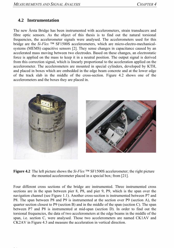
4.2 Instrumentation The new Årsta Bridge has been instrumented with accelerometers, strain transducers and fibre optic sensors. As the object of this thesis is to find out the natural torsional frequencies, the accelerometer signals were analysed. The accelerometers used for this bridge are the Si-Flex ™ SF1500S accelerometers, which are micro-electro-mechanical-systems (MEMS) capacitive sensors [2]. They sense changes in capacitance caused by an accelerated mass moving between two electrodes. Based on these changes, an electrostatic force is applied on the mass to keep it in a neutral position. The output signal is derived from this correction signal, which is linearly proportional to the acceleration applied on the accelerometer. The accelerometers are mounted in special cylinders, developed by KTH, and placed in boxes which are embedded in the edge beam concrete and at the lower edge of the track slab in the middle of the cross-section. Figure 4.2 shows one of the accelerometers and the boxes they are placed in.

Figure 4.2 The left picture shows the Si-Flex ™ SF1500S accelerometer; the right picture the mounted accelerometer placed in a special box; from [21].

Four different cross sections of the bridge are instrumented. Three instrumented cross sections are in the span between pier 8, P8, and pier 9, P9, which is the span over the navigation channel (see Figure 1.1). Another cross-section is instrumented between P7 and P8. The span between P8 and P9 is instrumented at the section over P9 (section A), the quarter section closest to P9 (section B) and in the middle of the span (section C). The span between P7 and P8 is instrumented at mid-span (section D). In order to find out the torsional frequencies, the data of two accelerometers at the edge beams in the middle of the span, i.e. section C, were analysed. Those two accelerometers are named CK1AV and CK2AV in Figure 4.3 and measure the acceleration in vertical direction.


25

Figure 4.3 Instrumented cross-section C; from [21].

CK2

CK1

CK7

CK4

CK5

CK6

CK3

Tra

nsv

ersal stra

in tra

nsd

ucers

Longitu

din

al stra

in tra

nsd

ucers

Connectio

n b

ox

Accelero

meters

CKCB

CK3AV

CK4AH

CK1AV

CK2AV

Ped

estrian a

nd cy

cle path


26

4.3 Fourier Series and the Fast Fourier Transform Each periodic signal is composed of sine waves with different amplitude, phase and frequency as discovered by Baron Jean Baptiste de Fourier. An arbitrary periodic signal can therefore be mathematically described by a sum of sine-waves, the so-called Fourier-Series. Using the Euler identity to express cosine and sine, the Fourier Series of a signal x(t) is transformed to its exponential form and becomes:

∑∞

∞−=

=k

tkkatX 0ie)( ω (4.1)

with the coefficients

∫−

−=0

0

0

π

π

i0 de)(π2

ω

ω

ωωttxa tk

k (4.2)

and the fundamental frequency 0

0π2

T=ω , where T0 is the signals period.

In the above equation, and all following ones, the function itself is denoted with a lower case letter, its Fourier series or Fourier transform with an upper case letter. The coefficients ak are calculated by multiplying the function itself by exponential functions of different frequencies and integrating over one period. The magnitude of the coefficient ak depends on whether a frequency kω0 is actually contained in the signal x(t) and on the magnitude of the wave with that frequency. To describe a signal accurately, an infinite number of terms might be necessary, but to compute the Fourier series the amount of terms has to be limited and the signal approximated. When the signal is not continuous but discrete, like the acceleration signal sampled at a certain rate, the series becomes a discrete Fourier series. In this case, the integration over the period in equation (4.2) changes to a summation of the N discrete values of a period. Fourier analysis can also be applied for aperiodic sequences with the period T0 of a continuous, or period N of a discrete signal, approaching infinity. An aperiodic signal is described by a Fourier Transform. The Discrete Fourier Transform (DFT) of an aperiodic discrete signal, defined over the range 0 ≤ n ≤ N – 1, is

[ ] [ ]∑−

=

=1

0

2i-

eN

n

nkNnxkXπ

(4.3)

where 2π /N=Ω 0 describes the fundamental frequency, comparable to ω0 in (4.1) and (4.2). The DFT is a function of the frequency Ω(k)= k ⋅Ω0 and converges to being a continuous function with N→ ∞. In contrast to periodic signals, non-periodic signals are not composed of a few distinct frequencies, but their energy is distributed over a frequency range. In the frequency spectrum, the energy of the signal over the frequencies is displayed, i.e. the signal’s power spectral density (PSD). This density is the product of the transform and its complex conjugate. The peaks in the frequency spectrum indicate the frequencies with the highest spectral energy, which are the main components of the signal. Although the


27

processed signal is in reality aperiodic, it is in fact assumed periodic for the computation of the DFT with period N. For practical purposes N will of course not be infinite, as assumed in deriving equation (4.3), but have a finite value. The computation of a DFT can take a long time, as many values need to be calculated. Therefore, Fast Fourier Transform (FFT) algorithms have been developed to cut down computation time. As the exponential function in (4.3) is periodic, many values would be computed several times if a DFT algorithm was implemented. FFT algorithms make use of this fact and break the long DFT down into a number of shorter and simpler DFT’s which are then composed to the transform of the signal. To use these FFT algorithms the number of sample values must be a power of two. Those FFT algorithms are implemented in computer programs, such as MATLAB® and can be used for the transformation of both periodic and aperiodic signals.

4.4 Time and Frequency Domain The time and the frequency domain provide two ways of displaying the same signal. In the time domain, the amplitude of the signal is displayed over the time axis. An accelerometer signal is usually displayed in this way, as the acceleration is recorded over a certain time period. In the frequency domain, the amplitudes of the sinusoids, which the signal is composed of, are displayed over the respective frequencies. The two domains visualise different information of the same signal and the display of the signal can be changed from one domain to the other without loosing information. Mathematically, this change is conducted via Fourier transform and inverse Fourier transform. The frequency spectrum computed with a FFT covers a frequency range from the reciprocal of the time record T0, which can also be expressed by sample frequency fS divided by the number of samples N, to half the sample frequency:

Nf

Tf S==

0min

1 2max

Sff = (4.4)

Between those frequencies lie N/2 equally spaced frequencies. That means there are only half as many points in the frequency domain as in the time domain, because each point contains two pieces of information: phase and magnitude. Figure 4.4 shows the correlation between the two domains, viewing the signal as three-dimensional. This is achieved by decomposing a two dimensional signal, e.g. acceleration over time, into its sine-waves components.


28

Figure 4.4 Time and Frequency Domain; from [1].

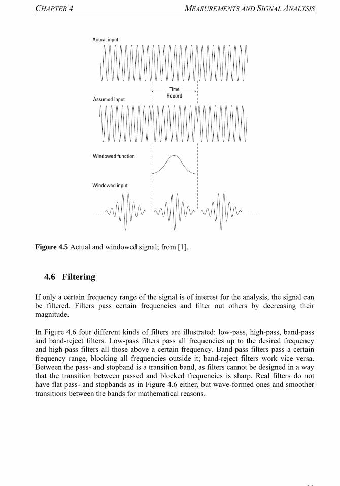
4.5 Windowing Windowing can be used to make the signal periodic over the sample period. Even a periodic signal might not be periodic over the recorded time span, if this is not a multiple of the signal’s period, and can therefore be windowed. For the computation it is assumed that the actual signal is a repetition of the recorded signal as illustrated in Figure 4.5. If this is non-periodic, the assumed input is a distorted signal with sharp transitions. Sharp transitions in one domain always cause wide spread results in the other domain. In this case that means there is no single peak at the sine-wave’s frequency in the frequency domain, but the energy is distributed over a range of frequencies, i.e. leakage occurs. To avoid this, the recorded signal is made periodic by multiplying it with a windowing function. Such a function attenuates the signal towards the beginning and end of the time record by multiplying it with zero at the ends. Although the windowed signal is altered, it still contains the same frequencies and the results of the spectral analysis are better than before. There are different windowing functions, which one is the most suitable depends on the problem. Popular windows are Hanning, Hamming and Flattop windows which all belong to the cosine window type. Some signals, like transient signals, do not need to be windowed, or alternatively can be windowed with a uniform window, because they already are zero at the boundaries of the time record.


29

Figure 4.5 Actual and windowed signal; from [1].

4.6 Filtering If only a certain frequency range of the signal is of interest for the analysis, the signal can be filtered. Filters pass certain frequencies and filter out others by decreasing their magnitude. In Figure 4.6 four different kinds of filters are illustrated: low-pass, high-pass, band-pass and band-reject filters. Low-pass filters pass all frequencies up to the desired frequency and high-pass filters all those above a certain frequency. Band-pass filters pass a certain frequency range, blocking all frequencies outside it; band-reject filters work vice versa. Between the pass- and stopband is a transition band, as filters cannot be designed in a way that the transition between passed and blocked frequencies is sharp. Real filters do not have flat pass- and stopbands as in Figure 4.6 either, but wave-formed ones and smoother transitions between the bands for mathematical reasons.


30

Figure 4.6 Filter types; from [16].

CHAPTER 5 RESULTS

31

5 Results

5.1 Bridge Properties The properties of a bridge span, which were used for the calculations, are shown in the following graphs. Those properties were obtained through a beam stress analysis for cross-sections every 0.5 m, starting at the point x = 0.25 m from the centre of a main span pier using the exact bridge geometry [21]. As the distance between those sections is 0.5 m, this was also chosen as distance between the calculation points in the finite difference model, starting at x = 0 m. The cross-section properties at those points were derived by linear interpolation between the values of the adjacent cross-section. The values for the section at x = 0 m were derived through extrapolation from the values at x = 0.25 m and x = 0.75 m. The graphs were drawn with MATLAB® and show the interpolated values that were used for the calculation. The material properties used for the graphs are the characteristic ones of concrete K60 with a cubic strength of 60 MPa. The values for Poisson’s ratio and mass density are the common ones for reinforced concrete.

• Modulus of elasticity E = 36 GPa

• Poisson’s ratio µ = 0.2

• Shear modulus ( )μ+=12

EG = 15 GPa

• Mass density ρ = 2 500 kg/m³

Figure 5.1 shows the distribution of the mass m along the bridge span in kg/m. It is derived by multiplying density by area, i.e. Am ⋅= ρ . In Figure 5.2 the torsional stiffness C in kNm² relating to the centre of gravity is displayed along the span. The torsional rigidity describes the resistance of a structure to St. Venant Torsion and is defined as a product of the shear modulus and the torsional moment of inertia, i.e. RIGC ⋅= . Figure 5.3 shows the warping stiffness CW in kNm4 along the span. CW describes the resistance of a structure to warping torsion and is calculated by multiplying the modulus of elasticity and the warping constant, i.e. SCW CEC ⋅= . For dynamic calculations the mass moment of inertia per unit length, J in kgm²/m, as shown in Figure 5.4 is needed. J is the product of the density and the polar moment of inertia, which is the sum of the moments of inertia related to the two elemental axis s and t perpendicular to the beam, i.e. ( )stP IIIJ +⋅=⋅= ρρ .

RESULTS CHAPTER 5

32

0 10 20 30 40 50 60 704

5

6

7

8

9

10

11x 104

length / m

mas

s / k

g/m

Figure 5.1 Mass distribution.

0 10 20 30 40 50 60 700.2

0.4

0.6

0.8

1

1.2

1.4

1.6

1.8x 109

length / m

C /

kNm

²

Figure 5.2 Torsional stiffness.

CHAPTER 5 RESULTS

33

0 10 20 30 40 50 60 703

4

5

6

7

8

9

10

11x 109

length / m

Cw

/ kN

m4

Figure 5.3 Warping stiffness.

0 10 20 30 40 50 60 701.3

1.4

1.5

1.6

1.7

1.8

1.9

2

2.1x 106

length / m

J /

kgm

2 /m

Figure 5.4 Mass moment of inertia per unit length.

RESULTS CHAPTER 5

34

5.2 Natural Torsional Frequencies from Single Span Bridge Model The natural torsional frequencies of the single span bridge model were calculated using equation (3.14), i.e.

[ ] [ ]( ){ } 02 =−′−′ ΦωBA (5.1) where [ ]A′ and [ ]B′ are the matrices (3.23) and (3.24), respectively, if the boundary conditions are chosen as fork bearings, and matrices (3.25) and (3.24) if they are assumed rigid. The span was divided into 156 sections, as explained in chapter 5.1, which results in matrices of the size 155×155. The natural torsional circular frequencies are the square-

roots of the eigenvalues 2jj ωω = .

The calculation of those eigenvalues was done with the eigs function in MATLAB®. The command [v,e]=eigs(A,k,’sm’) returns the k smallest eigenvalues e and the corre-sponding eigenvectors v of the matrix A. Eigenvalue calculations in MATLAB® are done using the Implicitly Restart Arnoldi Method (IRAM) [11]. The MATLAB® code for the composition of the matrices and the eigenvalue calculation of the single span bridge model is included in Appendix A. The calculation of the first three natural frequencies and the corresponding mode shapes yielded the results displayed in Table 5.1 and Figure 5.5, respectively. The mode shapes, i.e. the eigenvectors, were normalised to a maximum angle of one and drawn as unit mode shapes. To find out which boundary conditions describe the real situation best, the frequencies were calculated with both possibilities. In the first two columns of Table 5.1, results obtained for a single span with fork bearing are displayed; in the last two columns those calculated with a rigid support. The modulus of elasticity first chosen for the calculations was that of K60 concrete. Considering the pre-stressed tendons in the superstructure, the modulus of elasticity of the whole structure was found to be higher than that [21] and was therefore varied in the calculations. The modulus of elasticity was varied with the aim to come close to the measured frequencies. The mode shapes in Figure 5.5 are drawn for the frequencies given in the second column of Table 5.1.

Table 5.1 Natural torsional frequencies for different modulus of elasticity and different boundary conditions.

fn / Hz fork bearing rigid support n = E = 36 GPa E = 42.5 GPa E = 36 GPa E = 39.5 GPa

1 3.9143 4.2530 4.0503 4.2427 2 7.3180 7.9513 7.6750 8.0394 3 11.1144 12.0762 11.7561 12.3144

CHAPTER 5 RESULTS

35

0 10 20 30 40 50 60 70 78-1

-0.8

-0.6

-0.4

-0.2

0

0.2

0.4

0.6

0.8

1

length / m

norm

alis

ed to

rsio

nal a

ngle

/ ra

d

f = 4.25 Hz

f = 7.95 Hz

f = 12.08 Hz

Figure 5.5 Mode shapes number 1 to 3 of the single span bridge model.

To show the influence of the St. Venant and warping torsion on the natural frequencies, they have been calculated regarding only one component at a time. The results for the first 10 frequencies are shown in Table 5.2. In the first column the natural frequencies computed with regard to torsional stiffness and warping stiffness are displayed. The second column shows the frequencies obtained by considering only torsional stiffness; the third those obtained with regard to warping stiffness only. The last two columns show the relations between the results obtained with regard to both stiffness component to those with only one of the components. It is evident, that considering torsional warping only had a minor effect on low frequencies, but became significant for higher ones. The first natural frequency increased only 2% by considering torsional warping in comparison to neglecting it. In general, St. Venant torsional stiffness was determining for the low frequencies and warping stiffness for the high frequencies. In Figure 5.6 the first and fifth eigenmode calculated with only St. Venant torsional stiffness and with both St. Venant torsional and warping stiffness were plotted. The modes calculated without considering warping stiffness are the ones with the dashed lines. The figure shows that the influence of warping was smaller for the lower frequency.

RESULTS CHAPTER 5

36

Table 5.2 Comparison of n Eigenfrequencies of the single span bridge model.

n fn,torsion+warping fn, torsion fn, warping fn,torsion+warping

/ fn, torsion

fn,torsion+warping / fn, warping

1 3.9143 3.8191 0.4422 1.02 8.85 2 7.3180 6.9068 1.8595 1.06 3.94 3 11.1144 9.9413 4.2351 1.12 2.62 4 15.5752 13.0938 7.5024 1.19 2.08 5 20.7026 16.2929 11.7122 1.27 1.77 6 26.5703 19.4580 16.8960 1.37 1.57 7 33.2273 22.6507 22.9649 1.47 1.45 8 40.6914 25.8763 29.9752 1.57 1.36 9 48.9884 29.0939 37.9305 1.68 1.29

10 58.1227 32.2960 46.7862 1.80 1.24

0 10 20 30 40 50 60 70 78-1

-0.8

-0.6

-0.4

-0.2

0

0.2

0.4

0.6

0.8

1

length / m

norm

alis

ed to

rsio

nal a

ngle

/ ra

d

Figure 5.6 Eigenmodes number 1 and 5 with and without considering warping stiffness.

Modes without considering warping stiffness are the ones with dashed lines.

CHAPTER 5 RESULTS

37

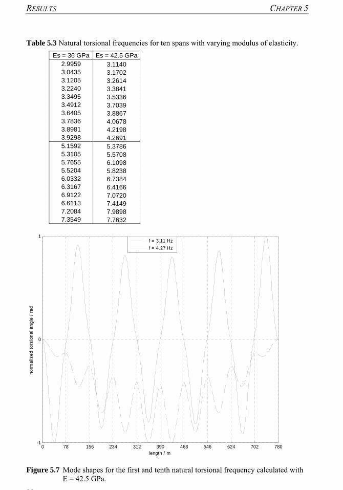
5.3 Natural Torsional Frequencies from Multi Span Bridge Model The multi span bridge model was developed with the intention to model the behaviour of the single span better and to eventually calculate the natural torsional frequencies of the whole bridge. In the first model, the natural torsional frequencies of a single span, which are higher than the frequencies of the complete bridge, were calculated. As the piers and the adjacent spans influence the vibration of the span, a model was developed taking this into consideration. The calculation was in principal the same as for the single span model, but using matrices (3.28) and (3.29) instead. Frequencies were calculated considering three spans, with the intention to model the span in the middle more accurately, considering the six straight spans and finally considering nine and ten spans, as the bridge has nine spans of equal length and two that are a bit shorter. In the ten span model one short span was neglected and the other end span modelled a bit longer. Both abutments were assumed very stiff and therefore modelled as rigid support. Two of the ten spans have a horizontal curvature, which was neglected in the calculations. The MATLAB® code for the multi span bridge model is included in Appendix B. Table 5.3 shows the results of the calculations for 10 spans with varying material properties. The pier’s modulus of elasticity remained unchanged, as it is not as heavily reinforced as the superstructure and was therefore not assumed equally stiff. The first ten and the next ten frequencies were close together with a gap in between them. The 10th and the 20th frequency were similar to the ones for a single span with a fork bearing. The mode shapes of those frequencies resemble sine-waves, where the torsional angles are zero at the points with a spring, which means the springs had no influence on those frequencies. The normalised mode shapes for the first and tenth frequency, calculated with a modulus of elasticity of 42.5 GPa, are displayed in Figure 5.7. The vertical dashed lines indicate the location of the piers.

RESULTS CHAPTER 5

38

Table 5.3 Natural torsional frequencies for ten spans with varying modulus of elasticity. Es = 36 GPa Es = 42.5 GPa

2.9959 3.1140 3.0435 3.1702 3.1205 3.2614 3.2240 3.3841 3.3495 3.5336 3.4912 3.7039 3.6405 3.8867 3.7836 4.0678 3.8981 4.2198 3.9298 4.2691 5.1592 5.3786 5.3105 5.5708 5.7655 6.1098 5.5204 5.8238 6.0332 6.7384 6.3167 6.4166 6.9122 7.0720 6.6113 7.4149 7.2084 7.9898 7.3549 7.7632

0 78 156 234 312 390 468 546 624 702 780-1

0

1

length / m

norm

alis

ed to

rsio

nal a

ngle

/ ra

d

f = 3.11 Hzf = 4.27 Hz

Figure 5.7 Mode shapes for the first and tenth natural torsional frequency calculated with

E = 42.5 GPa.

CHAPTER 5 RESULTS

39

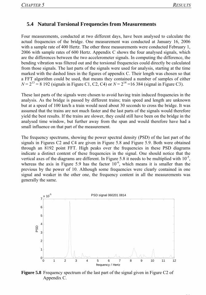
5.4 Natural Torsional Frequencies from Measurements Four measurements, conducted at two different days, have been analysed to calculate the actual frequencies of the bridge. One measurement was conducted at January 16, 2006 with a sample rate of 400 Hertz. The other three measurements were conducted February 1, 2006 with sample rates of 600 Hertz. Appendix C shows the four analysed signals, which are the differences between the two accelerometer signals. In computing the difference, the bending vibration was filtered out and the torsional frequencies could directly be calculated from those signals. The last parts of the signals were used for analysis, starting at the time marked with the dashed lines in the figures of appendix C. Their length was chosen so that a FFT algorithm could be used, that means they contained a number of samples of either N = 213 = 8 192 (signals in Figure C1, C2, C4) or N = 214 =16 384 (signal in Figure C3). These last parts of the signals were chosen to avoid having train induced frequencies in the analysis. As the bridge is passed by different trains; train speed and length are unknown but at a speed of 100 km/h a train would need about 30 seconds to cross the bridge. It was assumed that the trains are not much faster and the last parts of the signals would therefore yield the best results. If the trains are slower, they could still have been on the bridge in the analysed time window, but further away from the span and would therefore have had a small influence on that part of the measurement. The frequency spectrums, showing the power spectral density (PSD) of the last part of the signals in Figures C2 and C4 are given in Figure 5.8 and Figure 5.9. Both were obtained through an 8192 point FFT. High peaks over the frequencies in these PSD diagrams indicate a distinct content of these frequencies in the signal. One should notice that the vertical axes of the diagrams are different. In Figure 5.8 it needs to be multiplied with 10-5, whereas the axis in Figure 5.9 has the factor 10-6, which means it is smaller than the previous by the power of 10. Although some frequencies were clearly contained in one signal and weaker in the other one, the frequency content in all the measurements was generally the same.

0 1 2 3 4 5 6 7 8 9 10 11 120

1

2

3

4

5

6

7x 10

-5

frequency / Hertz

PS

D

PSD signal 060201 0814

Figure 5.8 Frequency spectrum of the last part of the signal given in Figure C2 of

Appendix C.

RESULTS CHAPTER 5

40

0 1 2 3 4 5 6 7 8 9 10 11 120

0.5

1

1.5

2

2.5

3x 10

-6

frequency / Hertz

PS

D

PSD signal 060201 1512

Figure 5.9 Frequency spectrum of the last part of the signal given in Figure C4 of Appendix C.

5.5 Comparison All the natural torsional frequencies lower than 5 Hz that were most prevalent in the analysis of all four signals are included in Table 5.4. Some higher frequencies, close to the ones that have been calculated, are included as well. As it is visible in the spectrums, the frequency content in the area of 8 Hz could not clearly be determined. There were peaks between 7.9 and 8.13 Hz in all signals, but none of the frequencies had clearly higher energy content than the surrounding ones. A comparison between the measured and calculated frequencies shows that there are computed results near the measured ones, both for the single span with fork bearing and E = 42.5 GPa and for the span with rigid support and E = 39.5 GPa. Considering the results of the multi span model it seems to be reasonable to assume fork bearings as supports. The second natural frequency could not clearly be determined in the measurements and the third one was not included. As shown in chapter 3.6 the method becomes more inaccurate for higher frequencies and yields frequencies lower than the accurate ones. In this case, the error would be large already for the third frequency, whereas the first and second could be found in the measurements. The calculations made with the multi span models yielded different results. A few of the calculated frequencies of the models with nine and ten spans were contained in the measurements, but in general the frequencies calculated with this model were too high. There were single frequencies in each model contained also in the measurements, but all the frequencies could never be calculated. Those frequencies that were found had other mode shapes than the ones calculated with an FEM model [21] and matched therefore accidentally.

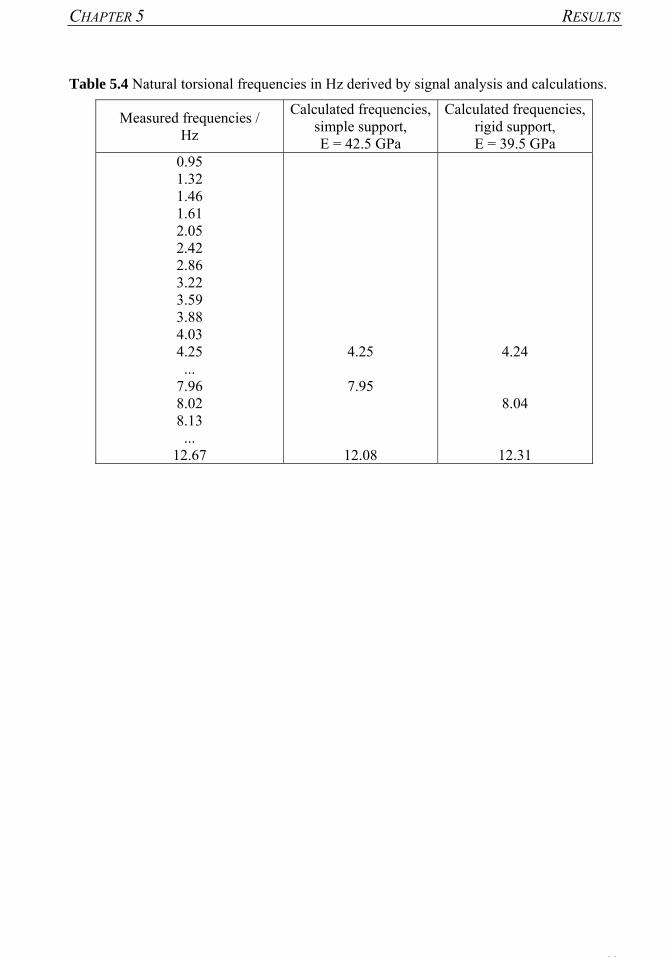
CHAPTER 5 RESULTS

41

Table 5.4 Natural torsional frequencies in Hz derived by signal analysis and calculations.

Measured frequencies / Hz

Calculated frequencies, simple support, E = 42.5 GPa

Calculated frequencies, rigid support, E = 39.5 GPa

0.95 1.32 1.46 1.61 2.05 2.42 2.86 3.22 3.59 3.88 4.03 4.25 ...

7.96 8.02 8.13 ...

12.67

4.25

7.95

12.08

4.24

8.04

12.31

DISCUSSION AND CONCLUSION CHAPTER 6

42

6 Discussion and Conclusion In this thesis, finite difference models for the calculation of the natural torsional frequencies of the new Årsta Railway Bridge were developed. Based on the partial differential equation for torsion of thin-walled elastic beams a single span bridge model and a multi span bridge model were implemented. The aim was to develop a rather simple model providing satisfactory results. Therefore, the following simplifications and approximations have been made for the calculations, which influence the results:

• The application of the differential equation for torsion for this kind of cross-section is only an approximation. As the cross-section is monosymmetrical, shear centre and the centre of gravity are not the same and torsion and horizontal bending coupled.

• The cross-section properties of the bridge used for the calculations are in relation to the centre of gravity. In the model the centre of gravity is straight whereas it varies in height along the bridge span in reality.

• The assumption that the cross-section of the bridge is non-deformable might also lead to erroneous results. Deformation of the cross-section can have a significant influence on the frequencies [4].

In the multi span bridge model the following further approximations have been made mainly regarding the bridge geometry:

• The length of the bridge in the model is not the same as in reality and one short end span has been neglected. This span was, together with abutment and pier, assumed very stiff and modelled as support with warping restraint, as well as the abutment on the other side.

• The piers were modelled as torsional springs. This, as well as the spring stiffness itself, is only an approximation. For the calculation of the spring stiffness the piers were assumed to be cantilever beams with properties as given in [21].

• The horizontal curvature of two of the bridge spans and thereby the coupled bending and torsional vibration was neglected.

The natural torsional frequencies calculated with the single span bridge model were close to frequencies contained in the measurements. The calculated first and second frequency were found in the measurements, whereas the third frequency was not contained, which means the calculations were rather inaccurate already for the third frequency. Even for the first and second frequency, the analysis done in this thesis is not sufficient to verify the calculation results with the measurements, as spans with two different boundary conditions yielded similar results. Further analysis of the measurements would be necessary to find out which of the frequencies belong to the vibrations of the whole bridge and which to the vibrations of the analysed single span only. It might be helpful to analyse the mode shapes to find out if the calculated and measured ones match. As the modulus of elasticity used in the calculations is much lower than the one that is obtained for the bridge through a more accurate finite element analysis [21], the calculated frequencies might be erroneous and match frequencies belonging to other mode shapes accidentally.

CHAPTER 6 DISCUSSION AND CONCLUSION

43

The calculations with the ten span bridge model yielded no useful results. The model overestimates the bridge stiffness as the lowest frequencies calculated with this model were much higher than the lowest measured ones. The method used in this thesis is therefore not suitable for calculating the natural torsional frequencies of such a multi-span box-girder bridge. The model was of course very approximate, but the frequencies should be lower nevertheless, if the model was suitable. The behaviour of the bridge is too complex to be calculated with this rather simple model and further improvements would be necessary, which would make the calculations with this model quite elaborate. In this case it seems necessary to implement a more accurate finite-element model, which can describe the bridge behaviour more accurately. For the calculation of the frequency of a simple beam the finite difference method usually yields good results. As the bridge is vibrating with its global modes, the frequencies that belong to only one span cannot easily be found in the measurements and further analysis would be necessary to verify the suitability of the method. However, as the vibrations of the single spans were not prevalent in this multi-span bridge the method seems to be suited better for the calculation of the frequencies of single span bridges. Warping had no significant influence on the low natural torsional frequencies of this bridge although the cross-sections with its edge beams are comparable to open cross-sections. The influence of warping decreases with the span length and increases for the higher frequencies, as shown in studies. In this case, the span is apparently long enough to keep the influence small for the low frequencies, which could therefore also be calculated satisfactorily without regarding warping stiffness.

LITERATURE

44

Literature [1] Agilent Technologies, Application Note 243, The Fundamentals of Signal Analysis,

1994-2000 [2] Colibrys Inc., Product description SF1500S, available on the internet

<http://www.colibrys.com/e/page/337/>, April 2006 [3] Francke, W.; Friemann, H., Schub und Torsion in geraden Stäben, Vieweg-Verlag,

Wiesbaden, 3. Auflage 2005 [4] Hamed, E., Frostig, Y., Free Vibrations of Multi-Girder and Multi-Cell Box Bridges

with Transverse Deformations Effects, Journal of Sound and Vibration, Vol. 279, No. 3-5, 2005, p. 699-722

[5] Jun, L, Rongying, S., Hongxing, H., Xianding, J., Coupled Bending and Torsional Vibration of axially loaded Bernoulli-Euler Beams including Warping Effects, Applied Acoustics, 65, 2004, p. 153-170

[6] Karoumi, R., Response of Cable-Stayed and Suspension Bridges to Moving Vehicles, Doctoral Thesis, Royal Institute of Technology (KTH), 1998

[7] Lehoucq, R.B., D.C. Sorensen, and C. Yang, ARPACK Users' Guide: Solution of Large-Scale Eigenvalue Problems with Implicitly Restarted Arnoldi Methods, 1997 <http://www.caam.rice.edu/software/ARPACK/> January 2006

[8] Li, D.-B., Chui, Y.H., Smith, I., Effect of Warping on Torsional Vibration of Members with open Cross Sections, Journal of Sound and Vibration, Vol.170, No 2, 1994, p. 270-275

[9] Maisel, B.I., Rowe, R.E., Swann, R.A., Concrete Box-Girders, The Structural Engineer, Vol.51, No.10, 1973, p. 363-376

[10] Mathews, J. H., Numerical Methods for Computer Science, Engineering and Mathematics, Prentice-Hall, Inc, Englewood Cliffs, New Jersey, 1987

[11] MathWorks, MATLAB function reference, 1984-2004 [12] Mehlhorn, G., Rützel H., Wölbkrafttorsion bei dünnwandigen Stahlbetonträgern, Der

Bauingenier 47, 1972, p. 430-438 [13] Orduña-Bustamente, F., Accurate Finite Difference Calculation of the Natural

Frequencies of Euler-Bernoulli Beams using Richardson Extrapolation, Journal of Sound and Vibration, Vol. 162, No 2, 1993, p. 361-367

[14] Petersen, C., Dynamik der Baukonstruktionen, Vieweg Verlag, Braunschweig/ Wiesbaden, 1. korrigierte Auflage 2000

[15] Pelinovsky, D., The Matlab Notebook v1.5.2, available on the internet <http://dmpeli.math.mcmaster.ca/Matlab/Math1J03/LectureNotes/Lecture4_1.htm> February 2006

[16] Smith, S.W., The Scientist and Engineer’s Guide to Digital Signal Processing, California Technical Publishing, 1997-98, available on the internet <http://www.DSPguide.com>

LITERATURE

45

[17] Subramahmanyam, K. B., Leissa, A. W., An Improved Finite Difference Analysis of Uncoupled Vibrations of Cantilevered Beams, Journal of Sound and Vibration, Vol. 98, No 1, 1985, p. 1-11

[18] Subrahmanyam, K. B., Kaza, K. R. V., Finite Difference Analysis of Torsional Vibrations of Pretwisted, Rotating Cantilever Beams with the Effect of Warping, Journal of Sound and Vibration, Vol. 99, No 2, 1985, p. 213-224

[19] Waldron, P., The Significance of Warping Torsion in the Design of straight Concrete Box Girder Bridges, Canadian Journal of Civil Engineering, Vol. 15, No 5, 1988, p. 879-889

[20] Waldron, P.; Kermani, B., Behaviour of Concrete Box-Girder Bridges of Deformable Cross-Section, Proceedings of the Institution of Civil Engineers Structures & Buildings, Vol. 99, Issue 2, 1993, p. 109-122

[21] Wiberg, J. Bridge Monitoring to Allow for Reliable Dynamic FE Modelling: A Case Study of the New Årsta Railway Bridge, Licentiate Thesis, Royal Institute of Technology (KTH), 2006

[22] Wlassow, W. S., Dünnwandige elastische Stäbe Band 1, VEB Verlag für Bauwesen Berlin, 2. übearbeitete Auflage 1964

[23] Zweidler, S., Hauswirth, D., Mathematische Behandlung von variablen Biegesteifigkeiten im konstruktiven Ingenieurbau, Semesterarbeit Mathematik, Fachhochschule Aargau, 2002

APPENDIX A

46

Appendix A

MATLAB® Code for the Calculation with the Single Span Bridge Model The following shows the MATLAB® Code for the calculation of the natural torsional frequencies of a single bridge span. Cscmean, TImean, SImean and RImean denote the following cross-section properties: warping constant, moment of inertia relating to elemtal axis t and s, and torsional moment of inertia, respectively. They have the ending mean because they were calculated as mean values of the given cross-section properties as explained in chapter 5.1. Instead of including the material properties in the matrices as in chapter 3, the matrices were multiplied by the modulus of elasticity E, the shear modulus G and the mass density ρ later, to make it easier to change those values for the calculations. The matrices in this example have the size n×n, which means the bridge span was divided into n+1 sections. % column vectors for A and B matrix for i = 1:n a(i,1) = (0.5*Cscmean(i)+Cscmean(i+1)-0.5*Cscmean(i+2))/... (TImean(i+1)+SImean(i+1)); a(i,2) = (-6*Cscmean(i+1)+2*Cscmean(i+2))/(TImean(i+1)+SImean(i+1)); a(i,3) = (-2*Cscmean(i)+10*Cscmean(i+1)-2*Cscmean(i+2))/... (TImean(i+1)+SImean(i+1)); a(i,4) = (2*Cscmean(i)-6*Cscmean(i+1))/(TImean(i+1)+SImean(i+1)); a(i,5) = (-0.5*Cscmean(i)+Cscmean(i+1)+0.5*Cscmean(i+2))/... (TImean(i+1)+SImean(i+1)); b(i,1) = (0.25*RImean(i)+RImean(i+1)-0.25*RImean(i+2))/... (TImean(i+1)+SImean(i+1)); b(i,2) = (-2*RImean(i+1))/(TImean(i+1)+SImean(i+1)); b(i,3) = (-0.25*RImean(i)+RImean(i+1)+0.25*RImean(i+2))/... (TImean(i+1)+SImean(i+1)); end ac = a; bc = b; %consider boundary conditions %phi(0) = 0, d^2phi(0)/dx^2 = 0, same for x=l a(1,3) = a(1,3)-a(1,1); a(n,3) = a(n,3)-a(n,5); %phi(0) = 0, dphi(0)/dx = 0, same for x=l ac(1,3) = ac(1,3)+ac(1,1); ac(n,3) = ac(n,3)+ac(n,5); %modify columns to fit sparse matrices a(:,1) = [a(3:n,1); 0; 0]; a(:,2) = [a(2:n,2); 0]; a(:,4) = [0; a(1:n-1,4)]; a(:,5) = [0; 0; a(1:n-2,5)]; b(:,1) = [b(2:n,1); 0];

APPENDIX A

47

b(:,3) = [0; b(1:n-1,3)]; ac(:,1) = [ac(3:n,1); 0; 0]; ac(:,2) = [ac(2:n,2); 0]; ac(:,4) = [0; ac(1:n-1,4)]; ac(:,5) = [0; 0; ac(1:n-2,5)]; bc(:,1) = [bc(2:n,1); 0]; bc(:,3) = [0; bc(1:n-1,3)]; %set up matrices A = spdiags(a,-2:2,n,n); B = spdiags(b,-1:1,n,n); Ac = spdiags(ac,-2:2,n,n); Bc = spdiags(bc,-1:1,n,n); rho = 0.0025; %kg*10^-6 E=36000; G=E/(2*(1+poisratio)); %MN/m^2 %eigenvalues [ce36,cv36]=eigs([A*E/(rho*lambda^4)-B*G/(rho*lambda^2)],10,'sm'); o = sqrt(diag(cv36)); f36 = o/(2*pi); [ce36c,cv36c]=eigs([Ac*E/(rho*lambda^4)-Bc*G/(rho*lambda^2)],10,'sm'); o = sqrt(diag(cv36c)); fc36 = o/(2*pi); E=55000; G=E/(2*(1+poisratio)); %MN/m^2 [ce55,cv55]=eigs([A*E/(rho*lambda^4)-B*G/(rho*lambda^2)],10,'sm'); o = sqrt(diag(cv55)); f55 = o/(2*pi); [ce55c,cv55c]=eigs([Ac*E/(rho*lambda^4)-Bc*G/(rho*lambda^2)],10,'sm'); o = sqrt(diag(cv55c)); fc55 = o/(2*pi); %draw eigenmodes for i = 1:10 vect(:,i) = ce36(:,i)/norm(ce36(:,i),inf); end vect = [zeros(1,12); vect; zeros(1,12)]; figure(1), hold on x = [0:0.5:78];

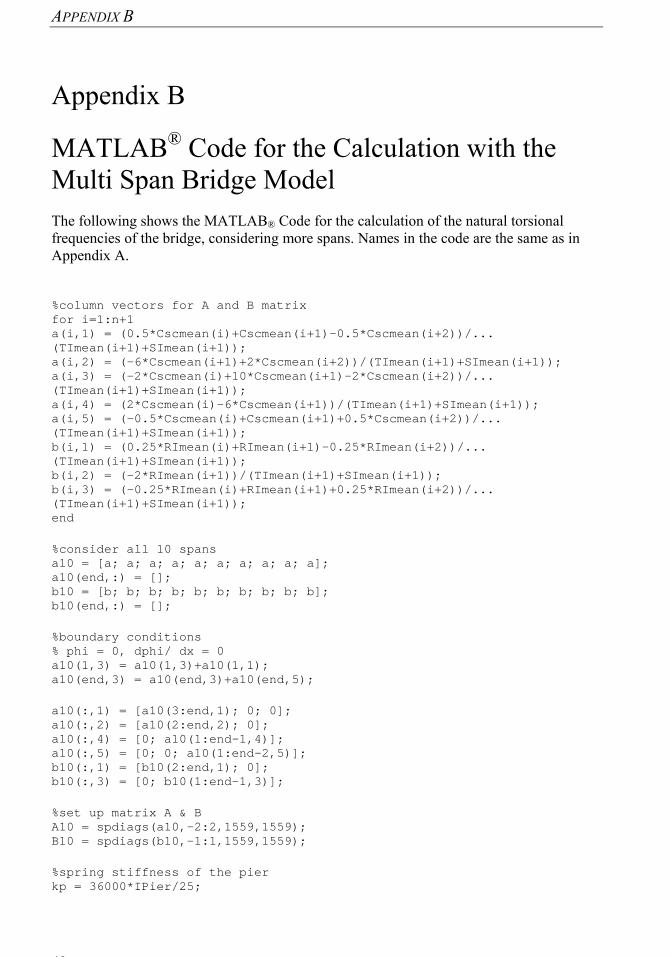
APPENDIX B

48

Appendix B

MATLAB® Code for the Calculation with the Multi Span Bridge Model The following shows the MATLAB® Code for the calculation of the natural torsional frequencies of the bridge, considering more spans. Names in the code are the same as in Appendix A. %column vectors for A and B matrix for i=1:n+1 a(i,1) = (0.5*Cscmean(i)+Cscmean(i+1)-0.5*Cscmean(i+2))/... (TImean(i+1)+SImean(i+1)); a(i,2) = (-6*Cscmean(i+1)+2*Cscmean(i+2))/(TImean(i+1)+SImean(i+1)); a(i,3) = (-2*Cscmean(i)+10*Cscmean(i+1)-2*Cscmean(i+2))/... (TImean(i+1)+SImean(i+1)); a(i,4) = (2*Cscmean(i)-6*Cscmean(i+1))/(TImean(i+1)+SImean(i+1)); a(i,5) = (-0.5*Cscmean(i)+Cscmean(i+1)+0.5*Cscmean(i+2))/... (TImean(i+1)+SImean(i+1)); b(i,1) = (0.25*RImean(i)+RImean(i+1)-0.25*RImean(i+2))/... (TImean(i+1)+SImean(i+1)); b(i,2) = (-2*RImean(i+1))/(TImean(i+1)+SImean(i+1)); b(i,3) = (-0.25*RImean(i)+RImean(i+1)+0.25*RImean(i+2))/... (TImean(i+1)+SImean(i+1)); end %consider all 10 spans a10 = [a; a; a; a; a; a; a; a; a; a]; a10(end,:) = []; b10 = [b; b; b; b; b; b; b; b; b; b]; b10(end,:) = []; %boundary conditions % phi = 0, dphi/ dx = 0 a10(1,3) = a10(1,3)+a10(1,1); a10(end,3) = a10(end,3)+a10(end,5); a10(:,1) = [a10(3:end,1); 0; 0]; a10(:,2) = [a10(2:end,2); 0]; a10(:,4) = [0; a10(1:end-1,4)]; a10(:,5) = [0; 0; a10(1:end-2,5)]; b10(:,1) = [b10(2:end,1); 0]; b10(:,3) = [0; b10(1:end-1,3)]; %set up matrix A & B A10 = spdiags(a10,-2:2,1559,1559); B10 = spdiags(b10,-1:1,1559,1559); %spring stiffness of the pier kp = 36000*IPier/25;

APPENDIX B

49

%matrix for spring stiffness of the piers C10 = zeros(1559,1559); C10(156,156) = 1; C10(312,312) = 1; C10(468,468) = 1; C10(624,624) = 1; C10(780,780) = 1; C10(936,936) = 1; C10(1092,1092) = 1; C10(1248,1248) = 1; C10(1404,1404) = 1; %material properties E=55000; G=E/(2*1.2); [v10,w10]=eigs([A10*E/(rho*lambda^4)-B10*G/(rho*lambda^2)+C10*kp/(rho*(SImean(157)+TImean(157))*lambda)],20,'sm'); o = sqrt(diag(w10)); f10_55=o/(2*pi)

APPENDIX C

50

Appendix C

Measurements of Acceleration

Figure C 1 Signal measured 06/01/16. Figure C 2 Signal measured 06/02/01 08:14.

Figure C 3 Signal measured 06/02/01 14:12. Figure C 4 Signal measured 06/02/01 15:12.

056.68

70.3-2

-1.5 -1

-0.5 0

0.5 1

1.5 2

time / s

acceleration / m/s2

032.36

59.7-2

-1.5 -1

-0.5 0

0.5 1

1.5 2

time / s

acceleration / m/s2

033.5

47-2.5 -2

-1.5 -1

-0.5 0

0.5 1

1.5 2

2.5

time / s

acceleration / m/s2

0 30.77

51.25-2

-1.5 -1

-0.5 0

0.5 1

1.5 2

2.5

time / seconds

acceleration / m/s2

analysis of a dynamically loaded beam bridge in torsion

Documents