analysis - monash universityusers.monash.edu.au/~dprice/research/spmhd/morris_phd.pdf · 3.4.2.1 w...
TRANSCRIPT

Analysis of Smoothed Particle
Hydrodynamics with
Applications
Thesis submitted for the degree of
Doctor of Philosophy
Department of Mathematics,
Monash University
Joseph Peter Morris
B.Sc.(Hons)
July 1996

Contents
Summary : : : : : : : : : : : : : : : : : : : : : : : : : : : : : : : : : : : : : : : : : : iv
Statement : : : : : : : : : : : : : : : : : : : : : : : : : : : : : : : : : : : : : : : : : : v
Publications : : : : : : : : : : : : : : : : : : : : : : : : : : : : : : : : : : : : : : : : : vi
Acknowledgements : : : : : : : : : : : : : : : : : : : : : : : : : : : : : : : : : : : : : vii
1 Introduction 1
1.1 The Fundamentals of SPH : : : : : : : : : : : : : : : : : : : : : : : : : : : : : : 3
1.1.1 The basic idea : : : : : : : : : : : : : : : : : : : : : : : : : : : : : : : : 4
1.1.2 The Momentum Equation : : : : : : : : : : : : : : : : : : : : : : : : : : 5
1.1.3 The Continuity Equation : : : : : : : : : : : : : : : : : : : : : : : : : : 6
1.1.4 The Thermal Energy Equation : : : : : : : : : : : : : : : : : : : : : : : 7
1.1.5 The Arti�cial Viscosity : : : : : : : : : : : : : : : : : : : : : : : : : : : 8
1.1.6 Thermal Conduction : : : : : : : : : : : : : : : : : : : : : : : : : : : : : 9
1.1.7 The Choice of Kernel : : : : : : : : : : : : : : : : : : : : : : : : : : : : 9
1.1.8 Variable Smoothing Length : : : : : : : : : : : : : : : : : : : : : : : : : 11
1.1.9 Initialising the Particles : : : : : : : : : : : : : : : : : : : : : : : : : : : 12
1.2 The Nearest Neighbour Problem : : : : : : : : : : : : : : : : : : : : : : : : : : 13
1.2.1 Locating neighbours with h constant : : : : : : : : : : : : : : : : : : : : 14
1.2.2 Locating neighbours with variable h : : : : : : : : : : : : : : : : : : : : 15
1.3 Time Integration : : : : : : : : : : : : : : : : : : : : : : : : : : : : : : : : : : : 16
1.3.1 An Overview : : : : : : : : : : : : : : : : : : : : : : : : : : : : : : : : : 16
1.3.2 The Predictor Corrector Scheme : : : : : : : : : : : : : : : : : : : : : : 17
2 Stability Analysis 19
2.1 Seeking the Source of the Instability : : : : : : : : : : : : : : : : : : : : : : : : 20
2.2 Stability Analysis and SPH : : : : : : : : : : : : : : : : : : : : : : : : : : : : : 21
2.2.1 The Linearised Equations : : : : : : : : : : : : : : : : : : : : : : : : : : 21
2.2.2 Obtaining a Dispersion Relation : : : : : : : : : : : : : : : : : : : : : : 23
2.2.2.1 The simple integral approximation : : : : : : : : : : : : : : : : 23
2.2.2.2 Using Poisson's Summation Formula : : : : : : : : : : : : : : : 23
2.2.2.3 Using Direct Summation : : : : : : : : : : : : : : : : : : : : : 24
2.2.3 Stability of Another Formulation : : : : : : : : : : : : : : : : : : : : : : 24
2.2.4 The Numerical Sound Speed : : : : : : : : : : : : : : : : : : : : : : : : 25
2.3 Results : : : : : : : : : : : : : : : : : : : : : : : : : : : : : : : : : : : : : : : : : 25
2.3.1 General Results : : : : : : : : : : : : : : : : : : : : : : : : : : : : : : : : 26
i

CONTENTS ii
2.3.2 A Pack of Camels : : : : : : : : : : : : : : : : : : : : : : : : : : : : : : 29
2.3.3 Numerical Results : : : : : : : : : : : : : : : : : : : : : : : : : : : : : : 30
2.3.3.1 The Spline Kernel, W
0
: : : : : : : : : : : : : : : : : : : : : : 31
2.3.3.2 The First Order \Camel", W
1
: : : : : : : : : : : : : : : : : : 37
2.3.3.3 A Tailor Made Kernel for < = �0:1, h = 1:2 : : : : : : : : : : 39
2.3.3.4 A Tailor Made Kernel for < = �1, h = 1 : : : : : : : : : : : : 41
2.3.3.5 A Kernel Tailor-made for < = 10, h = 1:2 : : : : : : : : : : : : 43
2.3.3.6 The Pressure Di�erencing Formulation of SPH : : : : : : : : : 45
2.4 Analysis for Variable Particle Spacing : : : : : : : : : : : : : : : : : : : : : : : 47
2.5 Stability Analysis with Viscosity : : : : : : : : : : : : : : : : : : : : : : : : : : 50
2.6 Two-Dimensional Stability Analysis : : : : : : : : : : : : : : : : : : : : : : : : 52
2.6.1 A Rectangular Grid : : : : : : : : : : : : : : : : : : : : : : : : : : : : : 52
2.6.2 A Hexagonal Grid : : : : : : : : : : : : : : : : : : : : : : : : : : : : : : 60
2.7 An Investigation of Alternative Kernels : : : : : : : : : : : : : : : : : : : : : : 63
2.7.1 Hexagonal Lattices : : : : : : : : : : : : : : : : : : : : : : : : : : : : : : 68
2.8 Three-Dimensional Stability Analysis : : : : : : : : : : : : : : : : : : : : : : : : 70
2.8.1 Cubic Lattices : : : : : : : : : : : : : : : : : : : : : : : : : : : : : : : : 71
2.8.2 Body-Centred Cubic Lattice : : : : : : : : : : : : : : : : : : : : : : : : : 75
2.9 Discussion : : : : : : : : : : : : : : : : : : : : : : : : : : : : : : : : : : : : : : : 78
2.9.1 Di�erent Methods for Dealing with Negative Stress : : : : : : : : : : : : 78
2.9.2 What Should You Do? : : : : : : : : : : : : : : : : : : : : : : : : : : : : 78
2.9.3 Dealing with Instabilities in 2D and 3D SPH : : : : : : : : : : : : : : : 79
2.10 Conclusion : : : : : : : : : : : : : : : : : : : : : : : : : : : : : : : : : : : : : : 80
3 Modelling MHD with SPH 82
3.1 The Various Approaches : : : : : : : : : : : : : : : : : : : : : : : : : : : : : : : 83
3.1.1 Modelling the Lorentz Force : : : : : : : : : : : : : : : : : : : : : : : : : 83
3.1.2 Updating the Magnetic Field : : : : : : : : : : : : : : : : : : : : : : : : 84
3.1.2.1 Evolving Particle Fields : : : : : : : : : : : : : : : : : : : : : : 85
3.1.2.2 Interpolating Particle Fluxes : : : : : : : : : : : : : : : : : : : 87
3.1.2.3 Other Possibilities : : : : : : : : : : : : : : : : : : : : : : : : : 89
3.2 The Arti�cial Viscosity : : : : : : : : : : : : : : : : : : : : : : : : : : : : : : : : 89
3.3 The Consistency of the Equations : : : : : : : : : : : : : : : : : : : : : : : : : : 90
3.4 Modelling MHD Shocks : : : : : : : : : : : : : : : : : : : : : : : : : : : : : : : 91
3.4.1 Perpendicular Shocks : : : : : : : : : : : : : : : : : : : : : : : : : : : : 92
3.4.2 Oblique Shocks : : : : : : : : : : : : : : : : : : : : : : : : : : : : : : : : 95
3.4.2.1 Slow Shocks : : : : : : : : : : : : : : : : : : : : : : : : : : : : 96
3.4.2.2 Fast Shocks : : : : : : : : : : : : : : : : : : : : : : : : : : : : : 101
3.5 The E�ect of Non-Zero Divergence : : : : : : : : : : : : : : : : : : : : : : : : : 102
3.6 Testing the Evolution of the Field in 2D : : : : : : : : : : : : : : : : : : : : : : 104
3.6.1 Shear Flow : : : : : : : : : : : : : : : : : : : : : : : : : : : : : : : : : : 105
3.6.2 A Single Eddy : : : : : : : : : : : : : : : : : : : : : : : : : : : : : : : : 105
3.6.2.1 Reproducing a Steady Result : : : : : : : : : : : : : : : : : : : 106
CONTENTS iii
3.6.2.2 Maintenance of a Solenoidal Field : : : : : : : : : : : : : : : : 107
3.7 Conclusion : : : : : : : : : : : : : : : : : : : : : : : : : : : : : : : : : : : : : : 112
4 Closed Pulsar Magnetosphere 113
4.1 The Model : : : : : : : : : : : : : : : : : : : : : : : : : : : : : : : : : : : : : : 118
4.2 Numerical Considerations : : : : : : : : : : : : : : : : : : : : : : : : : : : : : : 120
4.2.1 Detecting the Magnetosphere : : : : : : : : : : : : : : : : : : : : : : : : 120
4.2.2 Obtaining the Field Numerically : : : : : : : : : : : : : : : : : : : : : : 123
4.2.3 A Particle Representation of the Magnetosphere Boundary : : : : : : : 125
4.2.4 Modelling Accretion : : : : : : : : : : : : : : : : : : : : : : : : : : : : : 127
4.2.5 Modelling the Infalling Material : : : : : : : : : : : : : : : : : : : : : : 129
4.3 Test Cases : : : : : : : : : : : : : : : : : : : : : : : : : : : : : : : : : : : : : : : 130
4.3.1 Constant External Pressure : : : : : : : : : : : : : : : : : : : : : : : : : 130
4.3.2 Steady, Supersonic Accretion : : : : : : : : : : : : : : : : : : : : : : : : 133
4.4 Discussion and Conclusion : : : : : : : : : : : : : : : : : : : : : : : : : : : : : : 138
5 Shock Detection with SPH 139
5.1 The new switch : : : : : : : : : : : : : : : : : : : : : : : : : : : : : : : : : : : : 140
5.2 Test cases : : : : : : : : : : : : : : : : : : : : : : : : : : : : : : : : : : : : : : : 143
5.2.1 Stationary shock front : : : : : : : : : : : : : : : : : : : : : : : : : : : : 143
5.2.2 Cold streams colliding : : : : : : : : : : : : : : : : : : : : : : : : : : : : 146
5.2.3 A Shock Striking a Bubble : : : : : : : : : : : : : : : : : : : : : : : : : 148
5.3 Discussion and Summary : : : : : : : : : : : : : : : : : : : : : : : : : : : : : : 149
A Details of MHD Derivations 154
A.1 Obtaining the Consistency Equations : : : : : : : : : : : : : : : : : : : : : : : : 154
A.2 Deriving the Interpolated Particle Flux Approach : : : : : : : : : : : : : : : : : 155
B Halton Sequences 157
C A Form of SPH Boundary Condition 158
D The Errors at a Contact Discontinuity 161

iv
Summary
This thesis is a study of the numerical stability properties and several speci�c applications of
the method of Smoothed Particle Hydrodynamics (SPH).
Chapter 1 gives an overview of previous applications of SPH and outlines many improve-
ments that have been made to the original method. The theory upon which SPH is based is
presented and the standard approach to modelling pure hydrodynamics with SPH is described
in detail.
Chapter 2 presents extensive stability analysis of SPH. Previous work is reviewed and many
new results are presented. When using a formulation of SPH which conserves momentum
exactly, the motion of the particles is observed to be unstable to negative stress. The nature of
this instability is investigated and approaches which may be used to eliminate it are presented.
The properties of standard two-dimensional and three-dimensional SPH are studied in detail
and it is shown that the use of kernels with compact support introduces instabilities. In general
it is found that the stability properties of SPH improve as higher order spline interpolant
approximations to a Gaussian are used as kernels.
The modelling of magnetohydrodynamics (MHD) by SPH raises many technical issues.
Chapter 3 applies the acquired knowledge of SPH's stability properties to the speci�c case of
modelling MHD. Apart from potential numerical instabilities there are problems concerning
exact conservation of momentum and energy. The maintenance of the solenoidal �eld is also
crucial. These di�culties are investigated and solutions are suggested and tested.
In Chapter 4 a method whereby SPH may be used to model the interaction between a closed
magnetosphere and a surrounding, �eld-free plasma is presented. This method allows the
dynamic interaction of the magnetosphere and surrounding �eld-free plasma to be simulated.
This application involves exploiting SPH's ability to model complicated, dynamic boundaries.
In solving this problem several enhancements of SPH are introduced, including the development
of an accretion boundary condition at the magnetopause. The resulting three-dimensional,
time dependent method is tested against established time independent axisymmetric results.
Results obtained for some steady con�gurations are compared with previous work for closed
magnetospheres. Possible application of the technique to modelling of spin up and spin down of
pulsars is discussed. Other possible applications and enhancements of the method are outlined.
In Chapter 5 a new approach to detecting shocks is investigated. SPH simulates shocks by
using an arti�cial viscosity. Unlike Eulerian methods it is not convenient to reduce the e�ects
of viscosity by means of switches based on spatial gradients. In this chapter, a new form of
switch for the SPH viscosity is proposed. Each SPH particle has a viscosity coe�cient which
satis�es a di�erential equation designed to increase the coe�cient near a shock and cause it
to decay to a small value elsewhere. Examples applying the switch to one-dimensional shock
problems and to the case of a weak shock hitting a bubble con�rm that the switch is e�ective.

v
Statement
This thesis contains no material which has been accepted for the award of any other degree
or diploma in any university or other institution, and, to the best of my knowledge, contains
no material previously published or written by another person, except where due reference is
made in the text. Chapter 5 is the result of work done in collaboration with Prof. Dr Joseph
Monaghan.

vi
Publications
During the author's candidature, several articles relating to the subject matter of this thesis
were published or submitted for publication:
� Morris, J. P. (1994), \A Study of the Stability Properties of SPH", Applied Mathematics
Reports and Preprints, Monash University 94/22.
� Morris, J. P. (1994), \Modelling MHD with Particle Methods: An Overview of SPMHD",
in Cataclysmic Variables (proceedings of conference in Abano Terme, Italy), A.Bianchini,
M. Della Valle and M. Orio, eds.
� Morris, J. P. (1995), \An Overview of the Method of SPH", Technical Report Series,
Fachbereich Mathematik, Universit�at Kaiserslautern 152.
� Morris, J. P. (1996), \A Study of the Stability Properties of SPH", Publ. Astron. Soc.
Aust. 13, 97-102.
� Morris, J. P. (1995), \Modeling Pulsar Magnetospheres with SPH", Applied Mathematics
Reports and Preprints, Monash University.
� Morris, J. P. (1996), \Modeling Pulsar Magnetospheres with SPH", Proceedings of the
187th Meeting of the AAS, San Antonio, U.S.A.
� Morris, J. P. and Monaghan, J. J. (1996), \Shock Detection with SPH", submitted to J.
Comp. Phys.
� Morris, J. P. (1996), \Improved Kernels for use with SPH", Applied Mathematics Reports
and Preprints, Monash University

vii
Acknowledgements
I would like to thank my supervisor Prof. Dr Joseph Monaghan for his insight, advice and
collaboration. Thanks also to the members of my o�ce, J. Paul Hunter, Tony Papenfuss and
Daniel Prager, for many useful discussions and suggestions. Thanks also to Drs Uli Anzer and
Gerhard B�orner for suggesting the interesting problem of pulsar accretion and for inviting me
to visit the Max-Planck Institute for Astrophysics, Garching. I would like to thank Dr Tomasz
Plewa for allowing me to modify his PPM code to simulate the interaction of a weak shock
and a bubble of gas for comparison with the SPH results.
I would also like to thank all my fellow research students and the sta� of the Applied
Mathematics section. In particular, thanks to Barbara Innes for always knowing how things
can be done. Thanks also to my family and friends for their support.
In the course of my candidature I was supported �nancially by the Silver Jubilee Scholarship
of Monash University. Thanks to the British Council whose postgraduate bursary scheme made
my visit to the Department of Applied Maths and Theoretical Physics and the Institute of
Astronomy, Cambridge possible. Thanks also to Prof. Dr Helmut Neunzert for inviting me to
visit the Department of Mathematics of the University of Kaiserslautern.

Chapter 1
Introduction
\Particle Man, particle man.
Doing the things a particle can..."
They Might Be Giants, Particle Man
Smoothed Particle Hydrodynamics (SPH) is a Lagrangian, numerical method for modelling
uid dynamics. The uid is represented by particles, typically of �xed mass, which follow the
uid motion, advecting contact discontinuities, preserving Galilean invariance, and reducing
the computational di�usion of various uid properties including momentum. The equations
governing the evolution of the uid become expressions for inter-particle forces and uxes
when written in SPH form. It often possible to formulate SPH such that mass, momentum
and energy are conserved exactly. Several reviews of SPH have been published, including Benz
(1989) and Monaghan (1992). This chapter covers much of the theory upon which SPH is
based and introduces the reader to the standard equations used in most applications of SPH.
SPH was �rst developed to simulate astrophysical uid dynamics, in particular polytropes
(Lucy 1977, Gingold & Monaghan 1977). It is relatively easy to incorporate complicated
physical e�ects into the SPH formalism and thus SPH has been applied successfully to a
vast range of problems. These include elastic ow (Swegle 1992), magnetohydrodynamics (see
Chapt. 3), quasi-incompressible hydrodynamics (Monaghan 1994), gravity currents (Monaghan
1995c), the fracture of brittle solids (Benz & Asphaug 1993), the interaction of a weak shock
with a bubble of gas (x 5.2.3) and accretion onto a pulsar magnetosphere (Chapt. 4) to name
a few. SPH is an extremely versatile method, however, the errors in results can sometimes be
substantially larger than those obtained using methods tailored for a speci�c problem. There
are many problems, though, which can only be practically handled by SPH. Problems where
the geometry is highly irregular, or even dynamic, for example, are quite readily handled by
SPH. There are many applications where the Lagrangian nature of SPH can be exploited to
give accurate results without requiring the use of complicated grid re�nement algorithms.
For example, in early implementations of SPH the global particle resolution length (smooth-
ing length) was decreased or increased depending on the average density of the system. There
are, however, many problems where the uid expands or contracts locally (Hernquist & Katz
1

INTRODUCTION 1 2
1989) and the resolution should follow these local variations if consistent accuracy is to be
maintained throughout space. This can be done easily with SPH by allowing each particle to
have its own smoothing length based on the local number density of particles. This approach
is described in x 1.1.8. A further consideration is that in many systems the contraction or
expansion need not necessarily be isotropic. For example, rotating astrophysical systems often
produce attened or �lamentary structures. Such structures suggest that the resolution should
itself be anisotropic. This can be achieved with SPH by allowing the resolution length to vary
with direction about each particle according to the derivatives of the velocity �eld (Fulbright,
Benz & Davies 1995, Shapiro, Martel, Villumsen & Owen 1996). Such a modi�cation is far
easier to implement with SPH than a grid based method. While the results obtained using an
anisotropic resolution length are very good, there can be problems with conservation of angular
momentum and the smoothing lengths themselves becoming disordered. The results obtained
in this thesis use either a constant resolution (chapters 2 and 3) or an isotropic resolution
length which varies in space and time (chapters 4, and 5).
The typical systems SPH was �rst applied to had very low dissipation. Later an arti�cial
viscosity was developed (x 1.1.5) to allow strong shocks to be simulated. At a shock front,
the viscosity provides the necessary dissipation to convert kinetic energy into heat. Away
from the shock front, however, this arti�cial viscosity can also lead to unphysical damping
of the uid motion. In Chapt. 5 this issue is discussed and a new switch for the viscosity is
introduced which can be used to introduce the viscosity only where it is needed. It can be
shown (Pongracic 1988, Meglicki, Wickramasinghe & Bicknell 1993) that the arti�cial viscosity
produces a shear and bulk viscosity. This result has been used to model the transfer of angular
momentum in accretion disks (Murray 1996). In this thesis, however, the standard arti�cial
viscosity is used only to provide the necessary smoothing at a shock front. In some applications
it may be necessary to use a di�erent form of arti�cial viscosity from the standard. In this
work the simulation of oblique magnetohydrodynamic shocks, for example, required a modi�ed
arti�cial viscosity (x 3.2).
Most astrophysical applications of SPH involve an isolated, often gravitationally bound,
cloud of gas with no de�nite boundary. Under these circumstances contributions from the
e�ective boundary of the uid are usually neglected. SPH has also been used to simulate
the energetic collision of large bodies (Pongracic 1988) where surface terms are often negli-
gible. There are circumstances where contributions from boundary terms should be included
to improve the accuracy of a simulation. Such terms are needed, for example, to improve
conservation of angular momentum when anisotropic smoothing lengths are employed (Owen
& Fisher 1994). Also, if a uid with a distinct boundary is modelled, boundary terms are often
necessary. There are several approaches to including such contributions. It is possible to de-
velop additional terms in the SPH summations which are non-zero only at the edge of the uid
(Randles & Libersky n.d.). Often it is more convenient to include special boundary particles
in the simulation to provide the contribution from the boundaries. Such boundary particles
have been used successfully to model solid surfaces interacting with quasi-incompressible ows
(Monaghan 1995b). Special boundary particles have also been considered in the modelling of
long-time evolution of accreting binaries (Bate 1995). In this thesis, boundary particles are
used to simulate accretion onto a closed pulsar magnetosphere (Chapt. 4).

INTRODUCTION: The Fundamentals of SPH 1.1 3
The application of SPH to a wide range of problems has lead to signi�cant extensions
and improvements to the original method. Until relatively recently, however, the numerical
analysis of SPH had lagged behind these developments. It is not straightforward to apply
the techniques developed to analyse grid-based Eulerian numerical methods to a Lagrangian
method where the particle con�guration can become disordered. Most tests of SPH, therefore,
have involved applying SPH to problems with established analytic or numerical solutions.
Results of linear wave propagation tests and shock tube simulations (Monaghan & Gingold
1983) using SPH suggest SPH is usually accurate to within several percent for the typical levels
of resolution employed in astrophysical simulations. Steinmetz & Mueller (1993) presents an
investigation of the capabilities and limitations of SPH which involves modelling oscillating
polytropes. They �nd that their approach to varying the smoothing length greatly reduces the
intrinsic numerical di�usion of SPH to much less than that of most multidimensional Eulerian
and Lagrangian schemes. There have been many comparisons between SPH and Eulerian
schemes (e.g. x 5.2.3 and Smith, Houser & Centrella (1996)).
Several authors have performed theoretical numerical analysis on SPH (Monaghan 1989,
Morris 1994, Balsara 1995, Meglicki 1995, Ben Moussa & Vila 1996a, Ben Moussa & Vila
1996b). This often involves considering relatively ordered con�gurations of particles to simplify
the analysis. The results obtained by such analyses may be used to understand the e�ectiveness
and limitations of SPH under idealised circumstances. This, in turn, can lead to a qualitative
understanding of the method's performance under more general circumstances. It is through
such studies that the stability, accuracy and convergence properties of SPH are becoming
understood. Investigations of the stability properties of SPH for ordered arrangements of
particles have appeared in Monaghan (1989), Morris (1994), Balsara (1995), Morris (1996b)
and Morris (1996a). Chapter 2 studies the stability properties of SPH in detail, reviewing
previous results and extending the theory.
Some work has been done to establish practical estimates of the errors present in SPH
simulations. For example, Meglicki (1995) discusses a \�gure of merit" which can be used to
estimate the error in the SPH estimate of derivatives. Ben Moussa & Vila (1996a) presents a
study of SPH's ability to evaluate second order derivatives. Recently, the convergence of SPH
for speci�c equations of state has been proven (Ben Moussa & Vila 1996b, Ben Moussa & Vila
1996c). The accuracy of SPH is touched upon in x 5.2.3 in connection with errors present at
contact discontinuities.
1.1 The Fundamentals of SPH
This section is intended to introduce the reader to the concepts of SPH which are fundamental
to the method. Similar introductions may be found in Monaghan (1992) and Benz (1989).
Slightly di�erent approaches are used by each author to obtain essentially the same equations.

INTRODUCTION: The Fundamentals of SPH 1.1.1 4
1.1.1 The basic idea
We start with the equation
A(r) =
Z
A(r
0
)�(r� r
0
)dr
0
: (1.1)
If we replace the delta function by an interpolating kernel W (r; h) we obtain an integral
interpolant of the function A(r)
A
i
(r) =
Z
A(r
0
)W (r� r
0
; h)dr
0
: (1.2)
The kernel W has the following properties:
Z
W (r� r
0
; h)dr
0
= 1 (1.3)
and
lim
h!0
W (r� r
0
; h) = �(r � r
0
): (1.4)
The integral interpolant, A
i
, can be thought of a smoothed version of the original function
A. This is the origin of \Smoothed" in SPH. The next step, is to approximate the integral
interpolant with a summation interpolant over a number of points (particles) r
b
in space:
A
s
(r) =
X
b
A
b
m
b
�
b
W (r� r
b
; h): (1.5)
The �eld quantities at particle b are denoted by a subscript b. The mass associated with
particle b is m
b
and so we see that the quantity m
b
=�
b
is the inverse of the number density
(ie- the speci�c volume) and is, in some sense, a volume element.
The density, for example, can be obtained using
�(r) =
X
b
m
b
W (r� r
b
; h): (1.6)
It is now possible to obtain an estimate of the gradient of the �eld (provided W is di�er-
entiable) simply by di�erentiating the summation interpolant:
rA
s
(r) =
X
b
A
b
m
b
�
b
rW (r� r
b
; h): (1.7)
In practice, however, it is more accurate to use:
rA =
1
�
[r(�A) �Ar�] ; (1.8)
=
1
�
a
X
b
m
b
(A
b
�A
a
)rW (r � r
b
; h); (1.9)
since here the gradient of A is more explicit and thus is less susceptible to particle disorder.
Similarly, while the divergence of v could be obtained using
r � v =
X
b
m
b
�
b
v
b
� rW (r � r
b
; h); (1.10)
it is more accurate to use:
r � v =
r � (�v) � v � r�
�
(1.11)
=
1
�
a
X
b
m
b
(v
b
� v
a
) � r
a
W (r� r
b
; h): (1.12)

INTRODUCTION: The Fundamentals of SPH 1.1.2 5
For brevity, we will now introduce the notation
W
ab
=W (r
a
� r
b
; h); (1.13)
and let r
a
W
ab
denote the gradient of W
ab
taken with respect to r
a
(the co-ordinates of
particle a). Also, quantities such as v
a
� v
b
shall be written v
ab
.
1.1.2 The Momentum Equation
If we move the particles with the velocity of the uid, then
dr
a
dt
= v
a
; (1.14)
and
dv
a
dt
= �
1
�
a
(rp)
a
; (1.15)
where the pressure is given by an equation of state. For example, if the gas is isothermal we
take
p = c
2
�; (1.16)
where c is the speed of sound, and for an ideal gas
p = ( � 1) �u; (1.17)
where is the ratio of speci�c heats and u is the internal energy. It is now a matter of choosing
an SPH representation of the pressure gradient. We could use (1.9) and obtain
(rp)
a
=
1
�
a
X
b
m
b
(p
b
� p
a
)r
a
W
ab
: (1.18)
For this expression, the force between particles is zero for constant pressure, and the stabil-
ity properties (see x 2.3.3.6) are quite appealing, but linear and angular momentum are not
conserved exactly. If, however, we use
rp
�
= r
�
p
�
�
+
p
�
2
r�; (1.19)
then we have
dv
a
dt
= �
X
b
m
b
�
p
a
�
a
2
+
p
b
�
b
2
�
r
a
W
ab
; (1.20)
and linear and angular momentum are conserved exactly, since the particle forces are equal and
opposite and act along the line joining their centres (provided that the kernel is symmetric).
This form is also preferable because it is quite straightforward to obtain a consistent energy
equation(see x 1.1.4), but there are many possible symmetric forms (Monaghan 1992). The
expression
rp
�
=
p
�
�
r
�
1
�
1��
�
+
1
�
2��
r
�
p
�
��1
�
; (1.21)
leads to
dv
a
dt
= �
X
b
m
b
�
p
a
�
a
�
�
b
2��
+
p
b
�
b
�
�
a
2��
�
r
a
W
ab
; (1.22)
while
rp = 2
p
pr
p
p; (1.23)

INTRODUCTION: The Fundamentals of SPH 1.1.3 6
gives
dv
a
dt
= �
X
b
m
b
2
p
p
a
p
p
b
�
a
�
b
r
a
W
ab
: (1.24)
1.1.3 The Continuity Equation
We can solve the continuity equation
d�
dt
= ��r � v; (1.25)
implicitly, taking advantage of the Lagrangian motion of the particles using
�
a
=
X
b
m
b
W
ab
: (1.26)
Since the number and masses of the particles remains constant, total mass is conserved. Under
some circumstances, such as nearly incompressible ow (Monaghan 1994), it is advantageous
to use
d�
a
dt
=
X
b
m
b
v
ab
� r
a
W
ab
; (1.27)
since this allows the densities to be set at each particle initially. This may be employed to
eliminate arti�cial oscillations at free surfaces (Monaghan 1995b). Also, normally the density
must be obtained �rst by a sum over all the particles before other quantities may be interpo-
lated (involving a second pass over the particles). Having a di�erential equation for � means
that it can be updated at the same time as other particle quantities and only one pass over
the particles is required to obtain all the required information. The main disadvantage is that
this expression does not conserve mass exactly, but this does not cause problems in many
applications. It can be computationally advantageous to use (1.27) for several time steps and
then correct the density by using (1.26).
Sources and sinks of matter are quite readily introduced. Consider a continuity equation
of the form
d�
dt
= ��r � v + f(r): (1.28)
Since, total mass is no longer conserved, the particle masses must be allowed to vary with
time. Taking the time derivative of (1.26) we �nd
d�
a
dt
=
X
b
m
b
dW
ab
dt
+
X
b
dm
b
dt
W
ab
: (1.29)
Since the SPH expression for (1.28) is
d�
a
dt
=
X
b
m
b
v
ab
� r
a
W
ab
+
X
b
m
b
�
b
f
b
W
ab
; (1.30)
we make the identi�cation
dm
b
dt
=
m
b
�
b
f
b
: (1.31)

INTRODUCTION: The Fundamentals of SPH 1.1.4 7
1.1.4 The Thermal Energy Equation
If we are modelling an ideal gas (1.17) we must solve for the thermal energy of each particle.
The equation for the evolution of thermal energy per unit mass is
du
dt
= �
�
p
�
�
r � v: (1.32)
We can simply translate this (using (1.12)) to the SPH expression
du
a
dt
=
�
p
a
�
a
2
�
X
b
m
b
v
ab
� r
a
W
ab
(1.33)
when using (1.20), this conserves total energy exactly. To see this, we must consider the rate
of change of kinetic energy resulting from (1.20). The total kinetic energy of the particles is
E
k
=
X
a
1
2
m
a
v
a
2
(1.34)
so the time rate of change is given by
dE
k
dt
=
X
a
m
a
v
a
�
dv
a
dt
; (1.35)
=
X
a
m
a
v
a
�
(
�
X
b
m
b
�
p
a
�
a
2
+
p
b
�
b
2
�
r
a
W
ab
)
; (1.36)
= �
X
a
X
b
m
a
m
b
�
p
a
�
a
2
+
p
b
�
b
2
�
v
a
� r
a
W
ab
: (1.37)
Simply swapping the dummy indices we obtain
dE
k
dt
= �
X
b
X
a
m
b
m
a
�
p
b
�
b
2
+
p
a
�
a
2
�
v
b
� r
b
W
ba
; (1.38)
= �
X
b
X
a
m
b
m
a
�
p
b
�
b
2
+
p
a
�
a
2
�
v
b
� (�r
a
W
ab
) (1.39)
since r
b
W
ba
= �r
a
W
ab
by antisymmetry. Thus, we can combine these results to get a
symmetric form and write
dE
k
dt
= �
1
2
X
a
m
a
X
b
m
b
�
p
a
�
a
2
+
p
b
�
b
2
�
v
ab
� r
a
W
ab
: (1.40)
Similarly, the time rate of change of the total internal energy resulting from (1.33) is
dU
dt
=
d
dt
X
a
m
a
u
a
; (1.41)
=
X
a
X
b
m
a
m
b
p
a
�
a
2
v
ab
� r
a
W
ab
; (1.42)
=
X
a
X
b
m
a
m
b
p
b
�
b
2
v
ba
� r
b
W
ba
; (1.43)
=
1
2
X
a
m
a
X
b
m
b
�
p
a
�
a
2
+
p
b
�
b
2
�
v
ab
� r
a
W
ab
: (1.44)
Total energy is conserved since it is the sum of the kinetic and internal energy of the particles.
INTRODUCTION: The Fundamentals of SPH 1.1.5 8
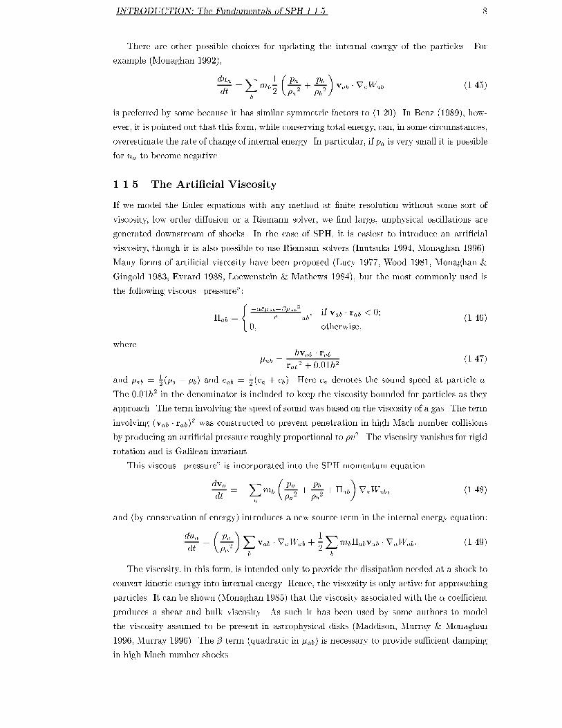
There are other possible choices for updating the internal energy of the particles. For
example (Monaghan 1992),
du
a
dt
=
X
b
m
b
1
2
�
p
a
�
a
2
+
p
b
�
b
2
�
v
ab
� r
a
W
ab
(1.45)
is preferred by some because it has similar symmetric factors to (1.20). In Benz (1989), how-
ever, it is pointed out that this form, while conserving total energy, can, in some circumstances,
overestimate the rate of change of internal energy. In particular, if p
a
is very small it is possible
for u
a
to become negative.
1.1.5 The Arti�cial Viscosity
If we model the Euler equations with any method at �nite resolution without some sort of
viscosity, low order di�usion or a Riemann solver, we �nd large, unphysical oscillations are
generated downstream of shocks. In the case of SPH, it is easiest to introduce an arti�cial
viscosity, though it is also possible to use Riemann solvers (Inutsuka 1994, Monaghan 1996).
Many forms of arti�cial viscosity have been proposed (Lucy 1977, Wood 1981, Monaghan &
Gingold 1983, Evrard 1988, Loewenstein & Mathews 1984), but the most commonly used is
the following viscous \pressure":
�
ab
=
(
���c�
ab
+��
ab
2
��
ab
; if v
ab
� r
ab
< 0;
0; otherwise,
(1.46)
where
�
ab
=
hv
ab
� r
ab
r
ab
2
+ 0:01h
2
(1.47)
and ��
ab
=
1
2
(�
a
+ �
b
) and �c
ab
=
1
2
(c
a
+ c
b
). Here c
a
denotes the sound speed at particle a.
The 0:01h
2
in the denominator is included to keep the viscosity bounded for particles as they
approach. The term involving the speed of sound was based on the viscosity of a gas. The term
involving (v
ab
� r
ab
)
2
was constructed to prevent penetration in high Mach number collisions
by producing an arti�cial pressure roughly proportional to �v
2
. The viscosity vanishes for rigid
rotation and is Galilean invariant.
This viscous \pressure" is incorporated into the SPH momentum equation
dv
a
dt
= �
X
b
m
b
�
p
a
�
a
2
+
p
b
�
b
2
+�
ab
�
r
a
W
ab
; (1.48)
and (by conservation of energy) introduces a new source term in the internal energy equation:
du
a
dt
=
�
p
a
�
a
2
�
X
b
v
ab
� r
a
W
ab
+
1
2
X
b
m
b
�
ab
v
ab
� r
a
W
ab
: (1.49)
The viscosity, in this form, is intended only to provide the dissipation needed at a shock to
convert kinetic energy into internal energy. Hence, the viscosity is only active for approaching
particles. It can be shown (Monaghan 1985) that the viscosity associated with the � coe�cient
produces a shear and bulk viscosity. As such it has been used by some authors to model
the viscosity assumed to be present in astrophysical disks (Maddison, Murray & Monaghan
1996, Murray 1996). The � term (quadratic in �
ab
) is necessary to provide su�cient damping
in high Mach number shocks.

INTRODUCTION: The Fundamentals of SPH 1.1.6 9
The arti�cial viscosity can, however, cause problems in regions of high shear. Here particles
are in relative motion, but one does not wish this motion to be critically damped. There are
di�erent approaches to correcting this problem, but most involve using some sort of switch
which detects the presence of a shock. See Chap. 5 for a detailed examination of this problem
and a new form of switch for the viscosity.
1.1.6 Thermal Conduction
Heat conduction may be introduced into a simulation either because it is present in the physics
of the real problem, or because it is needed to reduce excess heating (for example when cold
streams of gas collide). The standard di�erential equation for heat conduction is
@u
@t
=
1
�
r � �ru (1.50)
where � is the thermal conductivity. One could attempt to convert this directly into an SPH
form, but it would either require two sweeps over the particles (one for each gradient) or
directly involve second order derivatives. Estimation of second order derivatives with SPH
approximations which use second order derivatives of the kernel are very sensitive to particle
disorder (Brookshaw 1986, Monaghan 1988). So an alternative expression has been developed,
which only employs the gradient of the kernel:
@u
a
@t
=
X
b
m
b
(�
a
+ �
b
)(u
a
� u
b
)r
ab
� r
a
W
ab
�
a
�
b
(r
ab
2
+ 0:01h
2
)
: (1.51)
It can be shown (Monaghan 1995a) by taking a Taylor expansion about a particle, that this
does reduce to the heat equation. The contributions particles make to each other's heat uxes
are antisymmetric, so total heat is conserved.
If the conduction is intended to be arti�cial, it may be more convenient to use (Monaghan
1992):
@u
a
@t
=
X
b
m
b
(q
a
+ q
b
)(u
a
� u
b
)r
ab
� r
a
W
ab
��
ab
(r
ab
2
+ 0:01h
2
)
(1.52)
where q = �=� has the dimension of length squared per unit time. This allows us to readily
introduce conduction where it is needed by replacing q
a
+q
b
with
1
2
h(�c
ab
+4j�
ab
j). This term is
intended to provide conduction in those regions of the ow where large amounts of compression
(at shocks, for example) occurs, but could be improved upon by taking the approach outlined
in Chapt. 5 for shock detection.
1.1.7 The Choice of Kernel
Theoretically, the choice of kernel is arbitrary, provided it satis�es (1.3) and (1.4). We will
consider kernels of the form
W (r; h) =
1
h
�
f
�
r
h
�
; (1.53)
where � is the number of dimensions. The requirements of (1.3) and (1.4) can then be written
Z
f(s)dV = 1; (1.54)
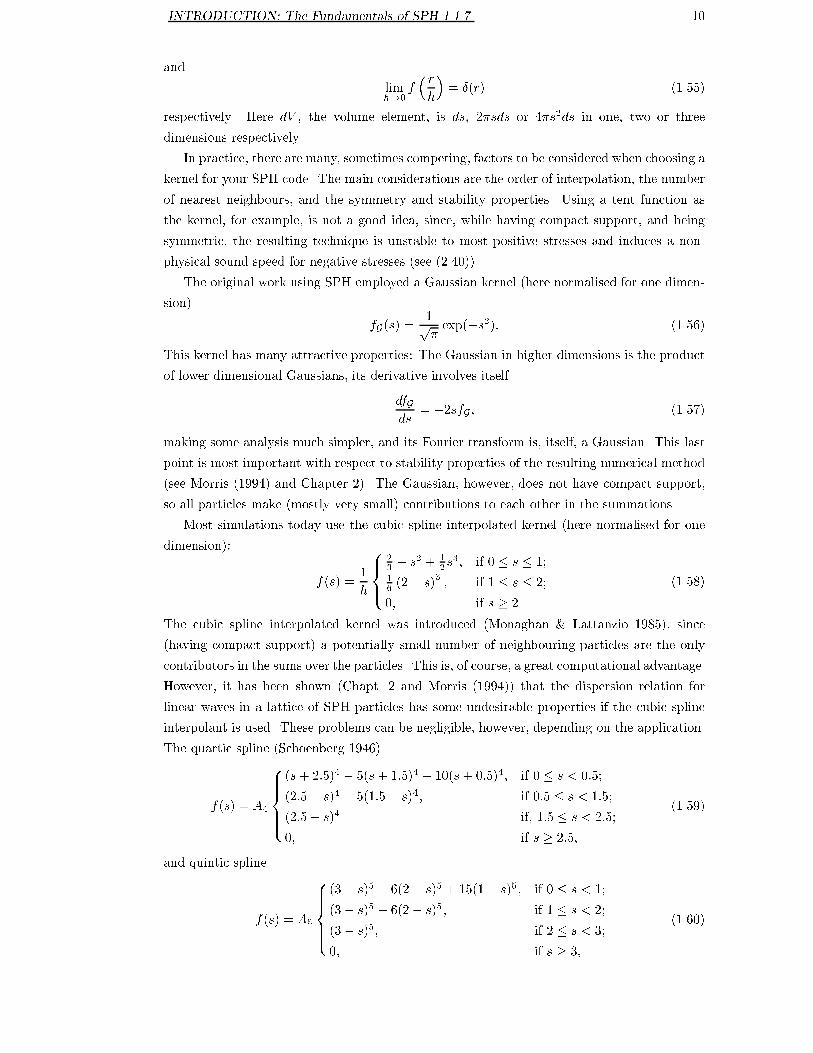
INTRODUCTION: The Fundamentals of SPH 1.1.7 10
and
lim
h!0
f
�
r
h
�
= �(r) (1.55)
respectively. Here dV , the volume element, is ds, 2�sds or 4�s
2
ds in one, two or three
dimensions respectively.
In practice, there are many, sometimes competing, factors to be considered when choosing a
kernel for your SPH code. The main considerations are the order of interpolation, the number
of nearest neighbours, and the symmetry and stability properties. Using a tent function as
the kernel, for example, is not a good idea, since, while having compact support, and being
symmetric, the resulting technique is unstable to most positive stresses and induces a non-
physical sound speed for negative stresses (see (2.40)).
The original work using SPH employed a Gaussian kernel (here normalised for one dimen-
sion)
f
G
(s) =
1
p
�
exp(�s
2
): (1.56)
This kernel has many attractive properties: The Gaussian in higher dimensions is the product
of lower dimensional Gaussians, its derivative involves itself
df
G
ds
= �2sf
G
; (1.57)
making some analysis much simpler, and its Fourier transform is, itself, a Gaussian. This last
point is most important with respect to stability properties of the resulting numerical method
(see Morris (1994) and Chapter 2). The Gaussian, however, does not have compact support,
so all particles make (mostly very small) contributions to each other in the summations.
Most simulations today use the cubic spline interpolated kernel (here normalised for one
dimension):
f(s) =
1
h
8
>
<
>
:
2
3
� s
2
+
1
2
s
3
; if 0 � s � 1;
1
6
(2� s)
3
; if 1 � s � 2;
0; if s � 2.
(1.58)
The cubic spline interpolated kernel was introduced (Monaghan & Lattanzio 1985), since
(having compact support) a potentially small number of neighbouring particles are the only
contributors in the sums over the particles. This is, of course, a great computational advantage.
However, it has been shown (Chapt. 2 and Morris (1994)) that the dispersion relation for
linear waves in a lattice of SPH particles has some undesirable properties if the cubic spline
interpolant is used. These problems can be negligible, however, depending on the application.
The quartic spline (Schoenberg 1946)
f(s) = A
4
8
>
>
>
<
>
>
>
:
(s+ 2:5)
4
� 5(s+ 1:5)
4
+ 10(s+ 0:5)
4
; if 0 � s < 0:5;
(2:5� s)
4
� 5(1:5� s)
4
; if 0:5 � s < 1:5;
(2:5� s)
4
if, 1:5 � s < 2:5;
0; if s � 2:5,
(1.59)
and quintic spline
f(s) = A
5
8
>
>
>
<
>
>
>
:
(3� s)
5
� 6(2� s)
5
+ 15(1� s)
5
; if 0 � s < 1;
(3� s)
5
� 6(2� s)
5
; if 1 � s < 2;
(3� s)
5
; if 2 � s < 3;
0; if s � 3,
(1.60)

INTRODUCTION: The Fundamentals of SPH 1.1.8 11
interpolants, have progressively better stability properties, but at an increased computational
cost, since the region of contributing neighbours is larger. Here A
4
and A
5
are normalisation
constants. It is possible (see x 2.7) to use a di�erent kernel for interpolation of density and
momentum. If appropriate kernels are chosen, it is possible to achieve improved stability
properties without an increase in the number of nearest neighbours.
Simply on account of their symmetry, all of these kernels interpolate to order h
2
accuracy
(since all odd moments are eliminated). It is possible, to formulate kernels which interpolate
to higher order accuracy by cancelling higher order moments in s. One such kernel is the
super-Gaussian (Gingold & Monaghan 1982). One possible disadvantage is that this kernel
is negative in a region of its domain and, thus, �
a
obtained by (1.26) could be negative in
some circumstances. Also, it is not clear that the super-Gaussian will give more accurate
interpolation than standard kernels once the particle positions become disordered.
1.1.8 Variable Smoothing Length
Changing the smoothing length in SPH corresponds to changing the numerical resolution. If
the uid modelled does not undergo substantial compression or rarefaction, constant h is su�-
cient. If particles become so distant, that they cease to interact, or so close that a large number
are within a smoothing length, h should be changed accordingly. All of the interpolation used
by SPH depends on having a su�cient number of particles within a smoothing length and the
speed of the computation depends on this number being relatively small. In one dimension,
the number of neighbours (including the \home" particle itself) should be about 5. In two
dimensions, it should be about 21 and in three dimensions, about 57. These numbers all cor-
respond to the number of neighbours on a cubic lattice with a smoothing length of 1:2 times
the particle spacing, and a kernel which extends to 2h (such as the cubic spline). If a kernel
with a larger area of compact support is used, the number of interacting neighbours should be
increased. There are many ways to dynamically change h such that the number of neighbours
is kept relatively constant.
The simplest approach is to let
h
a
= h
0
�
�
0
�
a
�
1
�
; (1.61)
where � is the number of dimensions. This only really makes sense if the particles are of equal
masses, since � is being used here as an estimate of the number density. The trouble with this
approach is that it requires �
a
to be known, before h
a
can be known. However, h
a
is needed
to obtain �
a
using either (1.26) or (1.27). The �
a
could be used from the previous step, but
this results in the smoothing length responding too slowly as a particle enters a shock. An
interesting and successful approach suggested by (Benz 1989) is to take the time derivative of
(1.61) and substitute the continuity equation
dh
dt
= �
1
�
h
�
d�
dt
(1.62)
=
1
�
hr � v (1.63)
This equation can then be integrated alongside the other di�erential equations. It may be

INTRODUCTION: The Fundamentals of SPH 1.1.9 12
prudent to reset h
a
according to (1.61) once �
a
is known, to ensure errors in the time integration
of h
a
do not lead to inappropriate smoothing lengths.
Since each particle now has its own smoothing length, each particle pair interaction must
have a smoothing length h
ab
associated with it. If we wish to conserve momentum exactly,
this must be done in such a way as to preserve the former symmetry of particle interactions:
W
ab
=W (r
ab
; h
ab
) (1.64)
where
h
ab
=
1
2
(h
a
+ h
b
); (1.65)
h
ab
= min(h
a
; h
b
); (1.66)
h
ab
= max(h
a
; h
b
); (1.67)
or h
ab
=
2h
a
h
b
(h
a
+ h
b
)
(1.68)
or we can average the kernels:
W =
1
2
fW (h
a
) +W (h
b
)g : (1.69)
There are advantages and disadvantages in using each of these. For example, for the arithmetic
mean in the limit of h
a
being dominant, h
ab
�
1
2
h
a
. This means that if, somehow, a particle
has an anomalously large h, it can overly smooth out interactions with surrounding particles.
This applies also when the maximum of the smoothing lengths is used. The geometric mean,
however, tends to 2h
b
as h
a
becomes large, so the resolution of the method is kept small.
Similarly, if the minimum of the smoothing lengths is used, the resolution of the method is
kept small. It is possible, however, that this approach may deprive a particle of the required
number of neighbours. Taking an average of the kernels may be a good compromise. In any
case, if variable smoothing length is being employed, the results obtained should be invariant
to the method used, provided the method has converged. The choice of combined smoothing
length also a�ects the speed with which nearest neighbours can be located (see x 1.2.2).
It should also be pointed out that it is not entirely consistent to allow h to vary in space
and time. The original SPH equations of motion were derived assuming h was a constant. It
is possible to rederive the SPH approximations, allowing h to vary (Bicknell 1991, Monaghan
1992). It has been found that, provided h varies on a scale similar to other variables, the
errors are of O(h
2
) (Hernquist & Katz 1989). More recent work (Hernquist 1993) suggests
that neglecting the correction terms when h is varied can lead to larger errors under some
circumstances.
1.1.9 Initialising the Particles
Initialising the SPH particles can sometimes require substantial care and e�ort. In some cases,
however, this may be because the initial conditions themselves are somewhat \arti�cial". In
most situations, we attempt to construct a \quiet" start, that is, a con�guration of particles
which does not have too much internal energy due to particles being placed in \unnatural"
ways. The approach taken depends very much on the precise application, but there are some
basic considerations to keep in mind.

INTRODUCTION: The Nearest Neighbour Problem 1.2 13
If the initial conditions involve discontinuities (either a shock or a contact discontinuity),
the interpolation used by SPH will smooth them out. This, typically, will lead to some extra
particle motion at the interface as the SPH particles respond to the pressure gradients induced
by the smoothed �elds. If (1.20) is used, we see that, even if the pressure is constant everywhere,
for the total force on each particle to be zero, all other particles must be placed symmetrically
about each other. In particular, at a contact discontinuity, where either the particle spacing or
particle masses will change, it is almost impossible to have an absolutely quiet start (see x D
for more detail). The noise can be minimised, however, by smoothing the initial conditions. In
the case of incompressible SPH (Monaghan 1994) these problems are avoided by using (1.27),
setting the density appropriately everywhere and subtracting the background pressure.
It may be convenient to place particles on a regular lattice, but care must be taken. Such a
lattice will have directions along which particles form straight lines. Compression along any of
these axes will cause particles to squeeze up into a dense line. If h is being reduced in response
to this compression, particles may lose \sight" of neighbours in parallel lines of particles. In
any case, the forces along such lines are arti�cially large, and eventually such lines buckle,
releasing substantial energy. If the initial velocity �eld naturally disturbs the initial, regular
lattice, these problems may be negligible.
Placing particles in a purely random fashion is certainly not advisable, since this results
in a great deal of noise which viscosity will convert into internal energy. As a compromise,
however, it is possible to use quasi-random sequences (such as the Halton sequences described
in x B) to choose the particle positions. Most such sequences select fairly evenly spaced points
in a unit interval. In many problems it is quite straightforward to develop a transformation
from a constant density on a unit interval to the desired density �eld. Residual noise may be
removed by introducing a relaxation term to the equations of motion, until the con�guration
has settled:
dv
dt
= ��v+ F: (1.70)
Here � is the co-e�cient of the damping and F includes the standard forces.
1.2 The Nearest Neighbour Problem
It has already been mentioned that, in practice, kernels with compact support are used in SPH
simulations. This is so that each particle has a �nite number of \neighbouring" particles which
make non-zero contributions to it. The problem still remains, however, to �nd these interacting
particles quickly. There are several solutions to this problem, and the optimal algorithm will
depend on the nature of the problem being solved. Here, we will consider methods which
assume that the SPH interactions are the only ones which need to be calculated. If, for
example, SPH is being used to provide hydrodynamics within a self-gravitating problem being
solved by a hierarchical tree-code (Hernquist & Katz 1989), the same structures used by the
tree-code to organise the gravitational approximations can readily be used to �nd nearest
neighbours to SPH particles. The methods we will consider involve creating a collection of
cells which cover real space and allow us to order and locate particles in space. These cells,
or grid, are simply used as a means of locating particles, and do not a�ect the results of the
simulation, only the speed with which it is obtained.

INTRODUCTION: The Nearest Neighbour Problem 1.2.1 14
1.2.1 Locating neighbours with h constant
Let us �rst consider the simpler case of constant smoothing length. In this case, all particles
have the same \interaction radius"
r
0
= s
k
h
0
(1.71)
where s
k
is the \extent" of the kernel in the co-ordinate s = r=h
0
. We can then divide the
computational domain into cells of width r
0
, and create lists of particles belonging to each
cell. A particle within a given cell, then, need only consider interactions with particles in
neighbouring cells. The lists of particles within each cell are most easily implemented as
linked lists. That is, there is a pointer to the �rst particle in a cell, and that particle then
points to the second particle and so on.
Let us consider the algorithm for one dimension in detail.
for i = 1 to n do
j = int((x
i
� x
min
)=r
0
)
next
i
= head
j
head
j
= i
Here head
j
is a pointer to the �rst particle in cell j, and is initially set to 0, while next
i
is a
pointer from particle i to the next particle in the linked list. Note that head
j
will point to 0
if cell j is empty and next
i
will point to 0 if it is the last particle in the list. Finding nearest
neighbours of particles i in cell j is now a much cheaper operation:
for cell = j � 1 to j + 1 do
k = head
cell
while (k 6= 0) do
consider particle k
k = next
k
However, in practice we do not consider an individual particle and search for its nearest
neighbours. It is much more e�cient to create a temporary list of particles in a given cell
and interacting neighbouring cells and evaluate the interactions between them. Also, since we
need only consider each pair of particles once, it is enough to consider the neighbouring cell to
one side of our home cell. The cell on the other side will consider the current home cell as its
neighbour and include it. For example, considering the SPH interactions for cell j, we create
a list of particles from cell j (the home cell) and cell j +1 (the neighbouring cell to the right):
i = 0
k = head
j
while (k 6= 0) do
i = i+ 1
list
i
= k
k = next
k
n
home
= i
k = head
j+1

INTRODUCTION: The Nearest Neighbour Problem 1.2.2 15
while (k 6= 0) do
i = i+ 1
list
i
= k
k = next
k
n
total
= i
The SPH contributions can be readily obtained by considering the pairs:
for i
1
= 1 to n
home
do
a = list
i
1
for i
2
= i
1
to n
total
do
b = list
i
2
consider particle a and b
This loop considers all the interactions between particles in the home cell (j) with each other
and with those particles in the neighbouring cell (j + 1). Since we don't wish to consider the
interactions between particles in the neighbouring cell with themselves, the �rst loop is over
n
home
particles while the second is over n
total
particles.
1.2.2 Locating neighbours with variable h
Once h is allowed to vary, the interaction radius for each particle is di�erent. In fact, since
we must apply some rule to obtain the e�ective h for a pair of particles, the interaction radius
will be di�erent for each pair of particles in general. Some of the ways smoothing lengths can
be combined appear in x 1.1.8. Only symmetric combinations are considered here since this is
necessary for exact conservation of momentum. The interaction length, for a pair of particles
is:
r
ab
= s
k
h
ab
: (1.72)
Now, if h does not vary by much in the simulation, it may be feasible to use the approach
described in the previous section, taking:
r
0
= max(r
ab
): (1.73)
However, as the variation in h is increased, there will be regions where large numbers of
particles (with small h) are clustered into single cells. Calculating the interactions between
these particles is very expensive. The cell sizes should stretch according to the local number
density of the particles. When using constant h, the cell boundaries are equispaced in real
space, since the particles are equispaced in real space. The most straightforward way to extend
this (using a Cartesian grid) is to consider cell boundaries which are equispaced in particle
rank space. That is, if we consider the particles ranked from left-most (say) to right-most
(ie- rank listed in x), the cell boundaries occur between every n
cell
-th particle. The choice of
n
cell
is made such that it is expected that one or two particles will be in each cell. In two
dimensions, for example, n
cell
=
p
n may be a good choice.
So, �rstly, the particles must be sorted lowest to highest in each dimension. The particles
must also be sorted at each time step, to obtain the new rank list and thence the cell grid. There
are many algorithms for sorting lists and they each have their advantages and disadvantages.
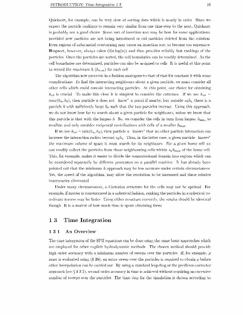
INTRODUCTION: Time Integration 1.3 16
Quicksort, for example, can be very slow at sorting data which is nearly in order. Since we
expect the particle rankings to remain very similar from one time-step to the next, Quicksort
is probably not a good choice. Some sort of insertion sort may be best for some applications,
provided new particles are not being introduced or old particles deleted from the solution.
Even regions of substantial overturning may cause an insertion sort to become too expensive.
Heapsort, however, always takes O(n log(n)) and thus provides reliably fast rankings of the
particles. Once the particles are sorted, the cell boundaries can be readily determined. As the
cell boundaries are determined, particles can also be assigned to cells. It is useful at this point
to record the maximum h (h
max
) for each cell.
The algorithm now proceeds in a fashion analogous to that of that for constant h with some
complications. To �nd the interacting neighbours about a given particle, we must consider all
other cells which could contain interacting particles. At this point, our choice for obtaining
h
ab
is crucial. To make this clear it is simplest to consider the extremes. If we use h
ab
=
max(h
a
; h
b
), then particle a does not \know" a priori if nearby, but outside s
k
h
a
there is a
particle b with su�ciently large h
b
such that the two particles interact. Using this approach,
we do not know how far to search about a given particle for neighbours, unless we know that
this particle is that with the largest h. So, we consider the cells in turn from largest h
max
to
smallest and only consider reciprocal contributions with cells of a smaller h
max
.
If we use h
ab
= min(h
a
; h
b
), then particle a \knows" that no other particle interaction can
increase the interaction radius beyond s
k
h
a
. Thus, in the latter case, a given particle \knows"
the maximum volume of space it must search for its neighbours. For a given home cell we
can readily collect the particles from those neighbouring cells within s
k
h
max
of the home cell.
This, for example, makes it easier to divide the computational domain into regions which can
be considered separately by di�erent processors on a parallel machine. It has already been
pointed out that the minimum h approach may be less accurate under certain circumstances.
Yet, the speed of the algorithm, may allow the resolution to be increased and these relative
inaccuracies eliminated.
Under many circumstances, a Cartesian structure for the cells may not be optimal. For
example, if matter is concentrated in a spherical fashion, ranking the particles in a spherical co-
ordinate system may be faster. Using either structure correctly, the results should be identical
though. It is a matter of how much time is spent obtaining them.
1.3 Time Integration
1.3.1 An Overview
The time integration of the SPH equations can be done using the same basic approaches which
are employed for other explicit hydrodynamic methods. The chosen method should provide
high order accuracy with a minimum number of sweeps over the particles. If, for example, �
must is evaluated using (1.26), an extra sweep over the particles is required to obtain � before
other interpolation can be carried out. By using a standard leap-frog or the predictor-corrector
approach (see x 1.3.2), second-order accuracy in time is achieved without requiring an excessive
number of sweeps over the particles. The time step for the simulation is chosen according to

INTRODUCTION: Time Integration 1.3.2 17
the CFL (Courant, Friedrichs & Lewy 1928) condition (see x 1.3.2) so the time-integration
is stable. In some applications, the time step required by the CFL condition varies greatly
between di�erent regions of the ow. In such cases it is possible to use individual time steps for
the particles. If the time steps are chosen to �t a hierarchy of powers of 2, then it is relatively
straightforward to integrate the equations of motion (Bate 1995).
A second order Runge-Kutta integrator has also been used with SPH. In this case (Benz
1984) it is possible to use adaptive time stepping. The time step is chosen to minimise an
estimate of the error in the integration within certain tolerances. The method requires more
sweeps over the particles per time step, however. In practice, it turns out that this time step
may be larger than that estimated using the CFL condition, and thus, this approach may have
de�nite computational advantages. As has been pointed out previously, one of the advantages
of using (1.27) is that it allows the density to be updated alongside other �eld quantities. It
may then be possible to integrate (1.27) for several time steps and then occasionally correct
with (1.26), to ensure conservation of mass.
Note that the stability properties discussed in Chapter 2 are independent of the time
integrator used. Chapter 2 deals with instabilities which are inherent in the SPH equations
for certain equations of state and certain kernels.
1.3.2 The Predictor Corrector Scheme
In this, one of the more popular integration schemes applied to SPH, the following equations
are used to obtain the �eld quantities at the next time step
~v
1=2
= v
0
+
�t
2
f
0
; (1.74)
~x
1=2
= x
0
+
�t
2
v
0
; (1.75)
�
1=2
= �(~x
1=2
); (1.76)
f
1=2
= f(~x
1=2
; ~v
1=2
; �
1=2
; : : :); (1.77)
v
1=2
= v
0
+
�t
2
f
1=2
; (1.78)
x
1=2
= x
0
+
�t
2
v
1=2
; (1.79)
x
1
= 2x
1=2
� x
0
; (1.80)
v
1
= 2v
1=2
� v
0
: (1.81)
Here, the superscripts refer to the time step index, and f is the force per unit mass (accelera-
tion). In practice we take f
0
� f
�1=2
, since this reduces the work required without changing
the order of the scheme.
The time step should be chosen to accommodate the CFL condition which, essentially,
states that the maximum rate of propagation of information numerically must exceed the
physical rate. In SPH, this translates to,
h
�t
� c
s
: (1.82)

INTRODUCTION: Time Integration 1.3.2 18
However, if viscosity is present, it should also be taken into account:
�t
cv
= min
a
h
c
a
+ 0:6(�c
a
+ �max
b
�
ab
)
: (1.83)
To ensure that the forces exerted on individual particles are integrated correctly, the time step
should also be less than
�t
f
= min
a
(
h
a
jf
a
j
): (1.84)
Here f
a
is a force per unit mass. So, a suitable time step for the scheme is
�t =
1
4
min(�t
cv
;�t
f
): (1.85)
The exact choice of coe�cients can be varied slightly. For example, simulations suggest (Mon-
aghan 1992)
�t = min(0:4�t
cv
; 0:25�t
f
) (1.86)
is adequate. If other processes are at work, for example heat conduction, then the time step
should be chosen to accommodate them using similar arguments. The main point to keep
in mind is that the natural SPH length scale is h. Other scales for the phenomenon under
consideration should be constructed from the relevant physical constants (as in (1.83)).

Chapter 2
Stability Analysis
\Nothing will come of nothing"
William Shakespeare, King Lear
The early applications of SPH (Lucy 1977, Gingold & Monaghan 1977) were to problems
involving a compressible gas which always had a positive gas pressure. The equations governing
the motion of the particles, when written in a form which conserves momentum exactly, result
in particles repelling each other with equal and opposite forces. As particles approach, the
density increases, the pressure increases, and the particles tend to repel each other. When
applied to di�erent problems where the stress can become negative, the momentum conserving
form of SPH is observed to become unstable to short wavelength perturbations. For negative
stress, the particles no longer repel, but attract. Each particle is, in e�ect, at the bottom
of a potential well, and it becomes possible for the particles to pair up and \slide" into each
other's wells, causing \clumping" initially and subsequently disrupting the solution. Recently
many people have commented upon this instability in connection with many problems (e.g.
elastic ow (Swegle 1992)), but much earlier Phillips & Monaghan (1985) had detected and
studied the problem in connection with smoothed particle magnetohydrodynamics (SPMHD).
The original subject of this thesis was the application of SPH to MHD (Chapt. 3), however, the
broader issue of stability analysis for SPH became the focus of the author's research for a time.
At the commencement of this thesis very little analytical work had been done in the study of
the stability properties of SPH and previous methods (Monaghan 1989) actually broke down
in the region where the stability we seek to understand �rst appears. In recent years, however,
there has been a substantial improvement in the understanding of the stability properties of
SPH (Morris 1994, Balsara 1995, Morris 1996b, Morris 1996a). This work seeks to extend the
stability analysis of SPH in order to not only understand the nature of potential instabilities
but to give insight into how methods giving most accurate results may be formulated.
One-dimensional stability analysis is used to gain insight into the nature of the instability re-
sulting from negative stress. The stability properties of two-dimensional and three-dimensional
SPH are also investigated in detail. It turns out that the use of spline interpolated kernels with
compact support introduces instabilities to the standard implementation of two-dimensional
19

STABILITY: Seeking the Source of the Instability 2.1 20
SPH. These instabilities are studied in detail and methods are suggested for dealing with them.
The possibility of using di�erent kernels to interpolate density and momentum is investigated.
One of the attractive attributes of SPH is its ability to give accurate solutions to a huge
range of problems. In dealing with potential numerical instability, it is important to ensure
that the resulting formulation is robust and accurate. In particular, approaches which attempt
to smooth out potential instabilities by increasing viscosity, may result in a less physical
solution and generally should be avoided. In fact, the e�ectiveness of viscosity in reducing
the instability may be quite limited (x 2.5). This report shows that, for many problems, it is
possible to modify SPH to be both stable and accurate. Naturally, the degree to which this is
possible and methods involved will depend upon the nature of the speci�c problem. Some of
these issues are explored further for the case of MHD in Chapt. 3.
2.1 Seeking the Source of the Instability
In order to understand the problem better we must seek the fundamental source of instability.
We have seen that the reported instability occurs when a stress tensor is implemented in a
form which conserves momentum exactly. In magneto-hydrodynamics, this implementation
takes the following form:
dv
a;i
dt
= �
X
b
m
b
�
p
a
�
2
a
+
p
b
�
2
b
�
r
a;i
W
ab
+
X
b
m
b
��
M
ij
�
2
�
a
+
�
M
ij
�
2
�
b
�
r
a;j
W
ab
; (2.1)
�
a
=
X
b
m
b
W
ab
(2.2)
p
a
= c
2
�
a
(2.3)
where
W
ab
=W (x
a
� x
b
; h) (2.4)
and the magnetic stress tensor
M
ij
=
1
�
0
�
B
i
B
j
�
1
2
�
ij
B
2
�
: (2.5)
Here, r
a;j
W
ab
denotes the j-th component of the gradient of W
ab
with respect to r
a
. We will
be considering one-dimensional ows initially, with symmetric kernels. Typically, we might
use a Gaussian kernel
W (x; h) =
1
h
p
�
e
�
�
jxj
h
�
2
(2.6)
or the cubic spline interpolant
W (x; h) =
1
h
8
>
>
<
>
>
:
2
3
�
�
jxj
h
�
2
+
1
2
�
jxj
h
�
3
; if 0 � jxj � h;
1
6
�
2�
�
jxj
h
��
3
; if h � jxj � 2h;
0; if jxj � 2h.
(2.7)
Choosing a symmetric kernel guarantees exact conservation of momentum, since inter-particle
forces form action-reaction pairs.

STABILITY: Stability Analysis and SPH 2.2 21
Let us consider the speci�c case of one-dimensional magneto-hydrodynamical ow, with
a constant magnetic induction B
0
parallel to the direction of the ow, say along the x-axis.
Since the magnetic induction is constant, the equations of magneto-hydrodynamics reduce to
those for hydrodynamics. However, the corresponding SPH equations behave di�erently. The
stress tensor becomes
M =
1
�
0
2
6
4
1
2
B
2
0
0 0
0 �
1
2
B
2
0
0
0 0 �
1
2
B
2
0
3
7
5
(2.8)
and the equations of motion for the particles may be written
dv
a
dt
= �
X
b
m
b
p
a
�
1
2�
0
B
2
0
�
2
a
+
p
b
�
1
2�
0
B
2
0
�
2
b
!
@W
ab
@x
a
; (2.9)
�
a
=
X
b
m
b
W
ab
; (2.10)
p
a
= c
2
�
a
: (2.11)
So, in this case, the SPH equations for magneto-hydrodynamical equations are equivalent to
those for pure hydrodynamical ow with the pressure adjusted by a constant. Similar analysis
may be done for any problem involving a stress tensor of the form similar to (2.5). So, the
stability properties of one-dimensional magneto-hydrodynamical SPH will be exhibited by the
equations
dv
a
dt
= �
X
b
m
b
�
p
a
�
2
a
+
p
b
�
2
b
�
@W
ab
@x
a
; (2.12)
�
a
=
X
b
m
b
W
ab
; (2.13)
p
a
= c
2
�
a
+ P; (2.14)
where P = �
1
2�
0
B
2
0
. In our analysis, however, it will be useful to allow P � 0 also.
2.2 Stability Analysis and SPH
2.2.1 The Linearised Equations
A simple way to analyse the stability of an implementation of SPH is to consider the dispersion
relation for sound waves propagating in a one-dimensional ow. We can imagine an in�nite
line of identical particles oscillating about a constant mean separation. Such a wave may be
described by
x
a
= a�x+Xe
i�
; (2.15)
v
a
= V e
i�
; (2.16)
�
a
= �
0
+Re
i�
(2.17)
where
� = ka�x� !t; (2.18)

STABILITY: Stability Analysis and SPH 2.2.2 22
with
m
a
= m; (2.19)
�
0
= m
X
b
W
ab
(2.20)
where, for the purposes of this analysis, we will simply write
W
ab
=W ([a� b]�x; h) : (2.21)
As short hand we will introduce the notation
e
a
� exp (ikx
a
� i!t) ; (2.22)
e
ba
� exp (�ikx
a
+ ikx
b
) : (2.23)
We now linearise (2.12) through (2.14) by substituting (2.17) and neglecting higher order terms
to obtain
�i!V = �
mc
2
�
0
X
b
�
2<X
@
2
W
ab
@x
2
a
(1� e
ba
)
+R(1� 2<)
@W
ab
@x
a
(1 + e
ba
)
�
; (2.24)
R = mX
X
b
@W
ab
@x
a
(1� e
ba
) (2.25)
where we have chosen
P = c
2
�
0
(<� 1) : (2.26)
< is, for the moment, an arbitrary constant. This choice of P gives
p
a
= c
2
�
0
�
�
a
�
0
� 1 + <
�
: (2.27)
Thus, if < > 0, then p
a
should be positive for small perturbations and if < < 0, then p
a
may
become negative. We can think of the quantity c
2
�
0
< as being the \background" pressure
upon which the linear wave perturbations occur. Combining (2.25), we obtain
!
2
=
2mc
2
<
�
0
X
b
(1� e
ba
)
@
2
W
ab
@x
2
a
+
m
2
c
2
�
2
0
(1� 2<)
X
b
(1 + e
ba
)
@W
ab
@x
a
X
b
0
(1� e
b
0
a
)
@W
ab
0
@x
a
: (2.28)
Substituting back for e
ba
and tidying up the summations we �nd
!
2
=
2mc
2
<
�
0
+1
X
j=�1
(1� e
�ik�xj
)
@
2
W
@x
2
(�xj; h)
+
�
mc
�
0
�
2
(1� 2<)
+1
X
j=�1
(1 + e
�ik�xj
)
@W
@x
(�xj; h)
�
+1
X
j
0
=�1
(1� e
�ik�xj
0
)
@W
@x
(�xj
0
; h): (2.29)

STABILITY: Stability Analysis and SPH 2.2.2.1 23
2.2.2 Obtaining a Dispersion Relation
In this section we consider several ways of analysing (2.29).
2.2.2.1 The simple integral approximation
This method has been used previously (Monaghan 1989) to give indications of stability prop-
erties for long wavelengths. The idea is to use the approximation:
X
a
f (a) �
Z
1
�1
f (x) dx: (2.30)
This is only valid for cases where f(a) varies su�ciently slowly with integral changes in a. We
then de�ne the Fourier transform of the kernel to be
U(k; h) =
Z
1
�1
e
�iku
W (u; h)du (2.31)
so
Z
1
�1
e
�iku
@
n
W
@u
n
du = (ik)
n
U(k; h) (2.32)
provided that
lim
u!�1
@
j
W (u; h)
du
j
= 0; for all 0 < j < n� 1. (2.33)
Using these expressions, we can write (2.29) in the form
!
2
= c
2
k
2
"
2m<
�
0
�x
U(k; h)�
�
m
��x
�
2
(2<� 1)U
2
(k; h)
#
(2.34)
Normally, for large
h
�x
, we take �
0
�
m
�x
. At this point, to keep results more general, we
will not make that approximation. Since we have used the approximation (2.30), the result
(2.34) will only apply for relatively small values of k, ie: those for which the integrand is slowly
varying. The limits of this approximation are explored in more detail in x 2.3.1.
2.2.2.2 Using Poisson's Summation Formula
Poisson's summation formula may be written
+1
X
n=�1
f
n
=
+1
X
l=�1
Z
+1
�1
f(x)e
�2�ilx
dx;where f(n) = f
n
: (2.35)
Using this formula we can write
+1
X
j=�1
e
�ik�xj
@
2
W
@x
2
(�xj; h)
=
+1
X
l=�1
Z
+1
�1
e
�ik�xu
0
@
2
W
@x
2
(�xu
0
; h)e
�2�ilu
0
du
0
; (2.36)
=
+1
X
l=�1
1
�x
Z
+1
�1
e
�i(k+
2�l
�x
)u
@
2
W
@u
2
du; (2.37)
=
+1
X
l=�1
�
(k +
2�l
�x
)
2
�x
U
�
k +
2�l
�x
; h
�
(2.38)

STABILITY: Stability Analysis and SPH 2.2.2.3 24
using (2.32). In a similar manner we can express all the summations of (2.29) in terms of sums
of Fourier transforms and obtain the result
!
2
=
2mc
2
<
�
0
�x
+1
X
l=�1
(
�
k +
2�l
�x
�
2
U
�
k +
2�l
�x
; h
�
�
�
2�l
�x
�
2
U
�
2�l
�x
; h
�
)
�
�
mc
�
0
�x
�
2
(1� 2<)
�
+1
X
l=�1
�
2�l
�x
U
�
2�l
�x
; h
�
+
�
k +
2�l
�x
�
U
�
k +
2�l
�x
; h
��
�
+1
X
l=�1
�
2�l
�x
U
�
2�l
�x
; h
�
�
�
k +
2�l
�x
�
U
�
k +
2�l
�x
; h
��
(2.39)
Some people might argue that this is not an improvement on (2.29), however, there are some
very useful results which we can obtain from this form. Such results will be derived and
discussed in x 2.3.1.
2.2.2.3 Using Direct Summation
If we make the assumption that the kernel, W, is even, then one can readily show that
!
2
=
2mc
2
<
�
0
X
j
(1� cos k�xj)
@
2
W
@x
2
(�xj; h)
+
�
mc
�
0
�
2
(1� 2<)
8
<
:
X
j
sin k�xj
@W
@x
(�xj; h)
9
=
;
2
: (2.40)
For a kernel with compact support, such as the spline interpolant (2.7), the summation is over
a �nite number of neighbours and may be done numerically with ease.
2.2.3 Stability of Another Formulation
It is possible to develop an alternative formulation to (2.12) which has stability properties
independent of the background pressure:
dv
a
dt
= �
X
b
m
b
p
b
� p
a
�
a
�
b
@W
ab
@x
a
; (2.41)
�
a
=
X
b
m
b
W
ab
; (2.42)
p
a
= c
2
�
0
�
�
a
�
0
� 1 + <
�
: (2.43)
Since the di�erences of the pressures are taken in the momentum equation, (2.41), the value
of < is irrelevant. However, the forces exerted upon the particles according to (2.41) no
longer form action-reaction pairs but are estimates of the local pressure gradient. Thus, this
formulation does not conserve momentum exactly, except in the continuum limit (ie: h ! 0
and in�nitely many particles). This pressure di�erence formulation has a very simple equation

STABILITY: Stability Analysis and SPH 2.2.4 25
governing its stability
!
2
= �
�
mc
�
0
�
2
2
4
+1
X
j=�1
�
1� e
�ik�xj
�
@W
@x
(�xj; h)
3
5
2
; (2.44)
which becomes
!
2
=
�
mc
�
0
�
2
2
4
+1
X
j=�1
sin k�xj
@W
@x
(�xj; h)
3
5
2
; (2.45)
if we use a symmetric kernel. The properties of (2.45) will be discussed in x 2.3.3.6.
2.2.4 The Numerical Sound Speed
The dispersion relation for the phase speed of hydrodynamic sound waves satisfying the exact
equations is
!
2
= c
2
k
2
: (2.46)
That is
c
2
=
!
2
k
2
: (2.47)
Thus, the numerical sound speed, c
num
, for our SPH approximation, will be given by
c
2
num
=
!
2
k
2
(2.48)
where !
2
is the dispersion relation for sound waves travelling in the SPH simulation. It is
useful to de�ne a scaled numerical sound speed, C
num
, de�ned by
C
2
num
=
c
2
num
c
2
=
!
2
k
2
c
2
(2.49)
where c is the analytic sound speed. Ideally, of course, C
num
should be as close to 1 as possible,
so that sound waves are propagated realistically. If C
2
num
becomes negative, the perturbations
in the numerical solution are no longer travelling waves, but are exponentially growing and
decaying disturbances. Thus, we have
C
2
num
�
� 0; stable; and
< 0; unstable.
(2.50)
For many applications, modelling the sound speed correctly (ie: C
2
num
� 1) is crucial. There
are situations, however, where the value of the numerical sound speed is not so important, yet
C
2
num
� 0 must be satis�ed at least.
2.3 Results
In this section we will draw some general results from the expressions derived in x 2.2.2 and
consider some speci�c cases. Keep in mind that it is the case where particles experience a
negative pressure (ie: < < 0) which people have found to be unstable. In particular, oscillations
with a wavelength of two particle separations usually become unstable �rst. Thus, we might
expect the instability to be present for
k �
�
�x
: (2.51)

STABILITY: Results 2.3.1 26
2.3.1 General Results
It is clear that the dispersion relation obtained using the Poisson summation formula (2.39) is
periodic in k with period 2�=�x. This is the result of aliasing, whereby waves of wavenumber
k and k + 2�=�x look identical at a series of points separated by �x. Thus, for the purposes
of stability analysis, we need only consider the stability of the \window" of wavenumbers
satisfying, say, 0 � k �
2�
�x
.
We can see that (2.39) reduces to the simple approximation (2.34) if we neglect all terms
but those for l = 0. This is not always a valid approximation. For a symmetric kernel, U(k; h)
will also be symmetric. Looking at (2.39) we see that, for a symmetric kernel and k = �=�x,
the magnitudes of the terms corresponding to l = 0 and l = �1 are the same. Thus, this
simple approximation is inappropriate for k � �=�x. Unfortunately, as we have seen, this is
the wavenumber at which the instability we are seeking to understand seems most severe. For
our purposes, then, we must use a more general approximation.
From now on we shall assume a symmetric kernel. Eq. (2.39) then becomes
!
2
=
2mc
2
<
�
0
�x
+1
X
l=�1
(
�
k +
2�l
�x
�
2
U
�
k +
2�l
�x
; h
�
�
�
2�l
�x
�
2
U
�
2�l
�x
; h
�
)
+
�
mc
�
0
�x
�
2
(1� 2<)
(
+1
X
l=�1
�
k +
2�l
�x
�
U
�
k +
2�l
�x
; h
�
)
2
(2.52)
Now, let us consider some of the properties of (2.52). It has been established experimentally
that the \problem" wavenumber is
�
�x
. For k =
�
�x
, (2.52), remembering that U is symmetric,
becomes
!
2
=
2mc
2
<
�
0
�x
+1
X
l=�1
(
�
�(2l + 1)
�x
�
2
U
�
�(2l+ 1)
�x
; h
�
�
�
2�l
�x
�
2
U
�
2�l
�x
; h
�
)
: (2.53)
This equation shows that, for wavenumber �=�x, the sign of !
2
, and hence C
2
num
, changes
sign with <. Thus, for any symmetric kernel, as the background pressure c
2
�
0
< changes sign,
it will change stability. There can be no kernel of this type which is stable for both signs of
<, using this implementation of SPH. The numerical results of x 2.3.3 support this. Thus, to
achieve general stability for di�erent background pressures, we must modify the kernel as <
changes sign. Let us consider the corresponding form of the direct summation (2.40) when
k = �=�x
!
2
=
2mc
2
<
�
0
X
j
(1� (�1)
j
)
@
2
W
@x
2
(�xj; h) ; (2.54)
=
4mc
2
<
�
0
1
X
j=�1
@
2
W
@x
2
(�x[2j + 1]; h) : (2.55)
We see that the sign of !
2
changes with that of < for k = �=�x as in (2.53). Let us consider

STABILITY: Results 2.3.1 27
(2.55) for the simple case where W (�xj; h) = 0 for jjj > 2. Then
!
2
=
8mc
2
<
�
0
@
2
W
@x
2
(�x; h) : (2.56)
So, for this case, the sign of
@
2
W
@x
2
(�x; h) must change when the background pressure changes
sign. This is particularly important to remember if we are seeking a kernel which changes
continuously with < to provide stability. The appropriate kernels for < being slightly positive
and slightly negative have di�erent signs for
@
2
W
@x
2
, so
@
2
W
@x
2
must be zero at the nearest neighbour
when < = 0 for continuity. In the case of the Gaussian, we �nd that !
2
= 0 when h =
p
2�x.
Thus, varying the smoothing length may be su�cient to ensure stability for this wavenumber.
A useful solution, however, must be stable for all wavenumbers.
We can see from the form of (2.52) and (2.40) that for any given h and k, C
2
num
varies
linearly with <. This includes the ideal case where C
2
num
is independent of < (ie: the terms
involving < cancel). In general, however, the best we can hope for is that C
2
num
varies slowly
with <. It is, therefore, informative to consider the quantity
@C
2
num
@<
, since this re ects the
degree of dependence of the stability properties on <. For su�ciently large < we have that
C
2
num
/ < where the constant of proportionality (for a given k and h) is
@C
2
num
@<
.
@C
2
num
@<
=
2m
k
2
�
0
�x
+1
X
l=�1
(
�
k +
2�l
�x
�
2
U
�
k +
2�l
�x
; h
�
�
�
2�l
�x
�
2
U
�
2�l
�x
; h
�
)
� 2
�
m
k�
0
�x
�
2
(
+1
X
l=�1
�
k +
2�l
�x
�
U
�
k +
2�l
�x
; h
�
)
2
; (2.57)
=
2m
k
2
�
0
X
j
(1� cos k�xj)
@
2
W
@x
2
(�xj; h)
� 2
�
m
k�
0
�
2
8
<
:
X
j
sin k�xj
@W
@x
(�xj; h)
9
=
;
2
: (2.58)
The limit of (2.52) as k approaches zero is of particular signi�cance. It is in this limit that
we expect our numerical method will resolve the wave best, since it corresponds to an in�nite
number of particles �tting into each wavelength. Let us consider the terms corresponding to
l = �1, 0 and 1 in (2.52) as k approaches zero and assume the other terms are negligible and
take m � �x�
0
.
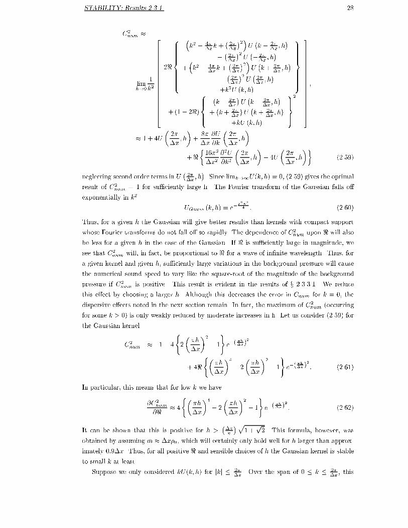
STABILITY: Results 2.3.1 28
C
2
num
�
lim
k!0
1
k
2
2
6
6
6
6
6
6
6
6
6
6
6
6
6
6
6
6
4
2<
8
>
>
>
>
>
>
>
<
>
>
>
>
>
>
>
:
�
k
2
�
4�
�x
k +
�
2�
�x
�
2
�
U
�
k �
2�
�x
; h
�
�
�
2�
�x
�
2
U
�
�
2�
�x
; h
�
+
�
k
2
+
4�
�x
k +
�
2�
�x
�
2
�
U
�
k +
2�
�x
; h
�
�
�
2�
�x
�
2
U
�
2�
�x
; h
�
+k
2
U (k; h)
9
>
>
>
>
>
>
>
=
>
>
>
>
>
>
>
;
+(1� 2<)
8
>
>
<
>
>
:
�
k �
2�
�x
�
U
�
k �
2�
�x
; h
�
+
�
k +
2�
�x
�
U
�
k +
2�
�x
; h
�
+kU (k; h)
9
>
>
=
>
>
;
2
3
7
7
7
7
7
7
7
7
7
7
7
7
7
7
7
7
5
;
� 1 + 4U
�
2�
�x
; h
�
+
8�
�x
@U
@k
�
2�
�x
; h
�
+ <
�
16�
2
�x
2
@
2
U
@k
2
�
2�
�x
; h
�
� 4U
�
2�
�x
; h
��
(2.59)
neglecting second order terms in U
�
2�
�x
; h
�
. Since lim
h!1
U(k; h) = 0, (2.59) gives the optimal
result of C
2
num
= 1 for su�ciently large h. The Fourier transform of the Gaussian falls o�
exponentially in k
2
U
Gauss
(k; h) = e
�
k
2
h
2
4
: (2.60)
Thus, for a given h the Gaussian will give better results than kernels with compact support
whose Fourier transforms do not fall o� so rapidly. The dependence of C
2
num
upon < will also
be less for a given h in the case of the Gaussian. If < is su�ciently large in magnitude, we
see that C
2
num
will, in fact, be proportional to < for a wave of in�nite wavelength. Thus, for
a given kernel and given h, su�ciently large variations in the background pressure will cause
the numerical sound speed to vary like the square-root of the magnitude of the background
pressure if C
2
num
is positive. This result is evident in the results of x 2.3.3.1. We reduce
this e�ect by choosing a larger h. Although this decreases the error in C
num
for k = 0, the
dispersive e�ects noted in the next section remain. In fact, the maximum of C
2
num
(occurring
for some k > 0) is only weakly reduced by moderate increases in h. Let us consider (2.59) for
the Gaussian kernel
C
2
num
� 1� 4
(
2
�
�h
�x
�
2
� 1
)
e
�
(
�h
�x
)
2
+ 4<
(
�
�h
�x
�
4
� 2
�
�h
�x
�
2
� 1
)
e
�
(
�h
�x
)
2
: (2.61)
In particular, this means that for low k we have
@C
2
num
@<
� 4
(
�
�h
�x
�
4
� 2
�
�h
�x
�
2
� 1
)
e
�
(
�h
�x
)
2
: (2.62)
It can be shown that this is positive for h >
�
�x
�
�
p
1 +
p
2. This formula, however, was
obtained by assuming m � �x�
0
, which will certainly only hold well for h larger than approx-
imately 0:9�x. Thus, for all positive < and sensible choices of h the Gaussian kernel is stable
to small k at least.
Suppose we only considered kU(k; h) for jkj �
2�
�x
. Over the span of 0 � k �
2�
�x
, this

STABILITY: Results 2.3.2 29
amounts to neglecting all but l = 0 and l = �1 in (2.39) to obtain
!
2
=
2mc
2
<
�
0
�x
(
�
k �
2�
�x
�
2
U
�
k �
2�
�x
; h
�
�
�
2�
�x
�
2
U
�
�
2�
�x
; h
�
+ k
2
U (k; h)
)
+
�
mc
�
0
�x
�
2
(1� 2<)
��
k �
2�
�x
�
U
�
k �
2�
�x
; h
�
+ kU (k; h)
�
2
: (2.63)
This approximation, by contrast with (2.34), is valid for all k satisfying 0 � k �
2�
�x
provided
kU(k; h) is negligible outside this band.
2.3.2 A Pack of Camels
We have seen that no single kernel can provide us with the stability we seek. We need some
way of modifying the present Gaussian shaped kernel. Any kernel, W (x; h) we choose must
have the following properties (in one-dimension):
Z
+1
�1
W (x; h)dx = 1; (2.64)
lim
h!0
W (x; h) = �(x) (2.65)
and, if we wish momentum to be conserved exactly,
W (x; h) =W (�x; h): (2.66)
We will take the kernel to be of the form:
W
0
(x; h) =
1
h
f
�
x
h
�
(2.67)
where, in the case of the cubic spline interpolated kernel,
f(s) =
8
>
<
>
:
2
3
� s
2
+
1
2
jsj
3
; if 0 � jsj � 1;
1
6
(2� jsj)
3
; if 1 � jsj � 2;
0; if jsj � 2.
(2.68)
We can now de�ne an in�nite series of symmetric kernels satisfying (2.65) of the following
form:
W
n
(x; h) =
A
n
h
�
x
h
�
2n
f
�
x
h
�
(2.69)
where A
n
is chosen to satisfy (2.65). For our choice of cubic spline kernel, (2.68), we �nd
A
n
=
(3 + 2n)(n+ 2)(n+ 1)(1 + 2n)
2(4
n+1
� 1)
(2.70)
giving A
0
= 1, A
1
= 3, A
2
=
30
9
, A
3
=
126
51
, and so on. Now we have a set of kernels which we
can combine to form a kernel with the necessary properties for stability,
W (x; h) =
N
X
j=0
B
n
W
n
(x; h) (2.71)

STABILITY: Results 2.3.3 30
where
N
X
j=0
B
n
= 1: (2.72)
Such kernels are typically not as accurate as W
0
, since they do not weight the central point
most heavily. In particular for small h=�x these cubic spline \camels" do not provide good
estimates of the density. For h=�x � 1, errors of several percent in the density are possible
for some choices of the coe�cients B
n
. The loss of accuracy is negligible, provided only small
B
n
for n > 1 is used.
We need to develop some method for choosing the co-e�cients B
n
such that the resulting
kernel has the desired stability properties. One approach would be to choose several matching
points that we want the numerical sound speed to pass through. For example, we might
require that !
2
= 0 at k
1
= �=�x and !
2
= c
2
k
2
2
at a suitably small k
2
. The �rst condition
ensures stability at the \troublesome" wavelength while the second leads to an appropriate
sound speed for small wavenumbers. We could then make an appropriate initial guess at the
kernel, say B
0
n
, and solve for our next iterate B
1
n
= B
0
n
+ �B
1
n
. Substituting the perturbed
co-e�cients into (2.40) and neglecting all but �rst order terms in the perturbations, we obtain
a set of linear equations for the perturbations. Each matching point provides another equation
such that the number of constraints should be the same as the number of free co-e�cients.
This system will be solvable provided certain attributes of (2.40) are respected.
Each particle has a number of particles which in uence it. Let such particles be called
neighbours. If a kernel with compact support is used, each particle has a �nite number of
neighbours. By symmetry the contribution from neighbours on either side of a particle is
identical in (2.40). No contribution to !
2
is made by the central particle. Each unique
neighbour makes a contribution in the form of
@
2
W
@x
2
and
@W
@x
. Thus, each unique neighbour can
provide two degrees of freedom to the quantity !
2
. However, if < = 0 then �rst term in (2.40)
vanishes, while, if < = 1=2 the second term vanishes. Thus, for < = 0 and < = 1=2 the number
of degrees of freedom is reduced by a factor of two. Care must be taken near these points to
ensure that the number of co-e�cients solved for (the number of degrees of freedom of the
kernel) does not exceed that of the system being solved. The form of !
2
is symmetric about
k =
�
�x
so care should be taken that equivalent matching points are not repeated. Generally, it
is safe to allow the kernel to have as many degrees of freedom as there are unique neighbours.
Having solved this system of linear equations for the perturbations, we repeat the process
solving for perturbations to B
1
n
and so on. This is essentially Newton's method and exhibits
quadratic convergence.
2.3.3 Numerical Results
For the purposes of obtaining numerical results, we will choose to take
�x = 1; (2.73)
m = 1: (2.74)

STABILITY: Results 2.3.3.1 31
2.3.3.1 The Spline Kernel, W
0
Using, (2.40) we can evaluate the scaled sound speed for a given kernel, h, < and k. Fig. 2.1
shows such results for the standard spline kernel, W
0
. Notice also that C
2
num
changes sign
Figure 2.1: Contour plot of C
2
num
for < vs k with h = 1:2 using W
0
. Contours are
separated by 0:1 with dotted lines denoting negative values.
at k = � and < = 0 as predicted. Indeed, the instability at k = � is the �rst to appear for
negative <, according to Fig. 2.1, in agreement with numerical experiment. Fig. 2.2 shows
Figure 2.2: A numerical run of an initial one percent perturbation, in the form of a
Gaussian pulse to the velocity, using W
0
with < = �1 and h = 1:2. One hundred
particles are used.
a simulation using this kernel and taking < = �1. After a short time (5 time units) we see
that the solution is developing oscillations with a wavelength of two particle separations (ie:
k = �). Let us consider (2.58) for this kernel. Fig. 2.3 shows a contour plot of the quantity
@C
2
num
@<
for h vs k. Careful inspection of Fig. 2.3 reveals that the largest gradient of C
2
num
as
a function of < for h = 1:2 occurs when k � �=2. For k � 0 the variation in C
2
num
is very

STABILITY: Results 2.3.3.1 32
slight. Thus, we will expect that, as < increases beyond 1, C
2
num
will increase most rapidly at
k � �=2, inducing strong dispersive e�ects. The theory also indicated that, if < became large
Figure 2.3: A contour plot of
@C
2
num
@<
for h vs k. The contours are 0:1 apart. The grey
areas are scaled with 0 white and �0:1 black.
enough in magnitude, C
2
num
for k = 0 would be proportional <. Fig. 2.4 shows that this is
indeed the case. We see C
2
num
increasing in proportion to <. Also, for a given value of < at
k � �=2, C
2
num
has a signi�cant maximum. Thus, the scheme is highly dispersive for large <.
A numerical simulation for the case of < = 10, Fig. 2.5, shows these dispersive e�ects. We
Figure 2.4: A contour plot of C
2
num
for < vs k with h = 1:2 for W
0
and a larger range
of < than for Fig. 2.1. Contours are separated by 1.
notice that smaller wavelength perturbations are travelling faster than the longer wavelengths.
This causes the Gaussian shape, consisting of a spectrum of wavelengths, to become askew.
It should be pointed out that this case is stable, but not particularly useful. The large forces
acting between the particles require a small time step to be used. The large background

STABILITY: Results 2.3.3.1 33
Figure 2.5: A numerical simulation using 200 particles and W
0
with < = 10 and
h = 1:2. The initial perturbation is a one percent Gaussian to the velocity.
pressure may also cause \arti�cial" non-linearity to occur. That is, the terms neglected in the
linearising of (2.12) through (2.14) to obtain (2.29) may become signi�cant before non-linear
e�ects are observed in the analytic wave equations. Let us now consider how the sound speed
Figure 2.6: A contour plot of C
2
num
for h vs k with < = 1 for W
0
. The contour lines
are separated by 0:1.
varies with the smoothing length h. Fig. 2.6 displays C
2
num
as a function of h and k for constant
< = 1. This is the \normal" un-adjusted background pressure corresponding to p = c
2
�
0
. We
notice that the squared sound speed does vary noticeably with h for h < 2 (the variations in
the sound speed itself are smaller). Beyond h = 2, the sound speed is much more reliable.
This is noteworthy since h = 1:2�x is the typical smoothing length employed by many people.
The corresponding plot for the pressure di�erencing formulation of SPH appears in Fig. 2.21.
In Fig. 2.3 we see that @C
2
num
=@< is actually negative for some values of k and h. In
particular, at k = 0 for h = 1:5 we have @C
2
num
=@< � �0:33. Therefore, we expect the
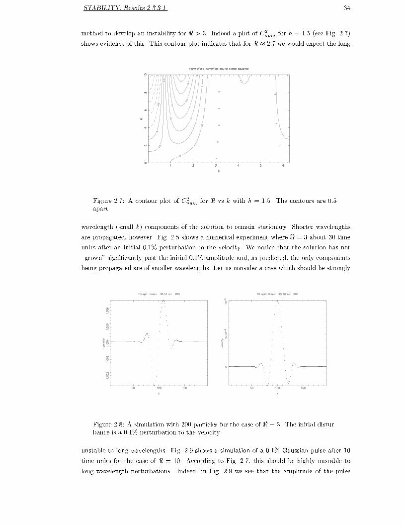
STABILITY: Results 2.3.3.1 34
method to develop an instability for < > 3. Indeed a plot of C
2
num
for h = 1:5 (see Fig. 2.7)
shows evidence of this. This contour plot indicates that for < � 2:7 we would expect the long
Figure 2.7: A contour plot of C
2
num
for < vs k with h = 1:5. The contours are 0:5
apart.
wavelength (small k) components of the solution to remain stationary. Shorter wavelengths
are propagated, however. Fig. 2.8 shows a numerical experiment where < = 3 about 30 time
units after an initial 0:1% perturbation to the velocity. We notice that the solution has not
\grown" signi�cantly past the initial 0:1% amplitude and, as predicted, the only components
being propagated are of smaller wavelengths. Let us consider a case which should be strongly
Figure 2.8: A simulation with 200 particles for the case of < = 3. The initial distur-
bance is a 0:1% perturbation to the velocity.
unstable to long wavelengths. Fig. 2.9 shows a simulation of a 0:1% Gaussian pulse after 10
time units for the case of < = 10. According to Fig. 2.7, this should be highly unstable to
long wavelength perturbations. Indeed, in Fig. 2.9 we see that the amplitude of the pulse

STABILITY: Results 2.3.3.1 35
has grown by a factor of 9 in this time. This example is a reminder of how an apparently
smooth solution can be very non-physical. This is especially true of the case of no propagation
where the solution may appear �ne (no instability develops) but has very little relevance to
reality. The kernel considered above is the standard cubic spline interpolant (2.7). If we use a
Figure 2.9: A simulation with 200 particles for the case of < = 9 after 10 time units.
The initial disturbance is a 0:1% perturbation to the velocity.
higher order spline interpolant, the Fourier transform will drop o� faster in kh. By (2.59) we
would expect the numerical sound speed to have a weaker dependence upon the background
pressure (at least for small k). For example, we could use a quartic spline interpolant (1.59)
which is continuous in the third derivative. A contour plot of @C
2
num
=@< for this smoother
kernel appears in Fig. 2.10. We see that the stability properties of this kernel depend much
Figure 2.10: A contour plot of @C
2
num
=@< for h vs k using a quartic spline interpolated
kernel. The contours are 0:1 apart. The grey areas are scaled with 0 white and �0:1
black.
less strongly upon the background pressure. The most negative point is near k = 0, h = 1:2

STABILITY: Results 2.3.3.1 36
where @C
2
num
=@< � �6:0 � 10
�2
. So with this kernel, we require < � 17 before the sound
waves are halted. Of course, the sound speed will be unacceptably reduced before this. This
is, however, for the worst choice of smoothing length. Fig. 2.11 displays similar contour plot
Figure 2.11: A contour plot of
@C
2
num
@<
for h vs k using the Gaussian kernel. The
contours are 0:1 apart. The grey areas are scaled with 0 white and �0:1 black (notable
by their absence).
for the Gaussian kernel (2.6). As we might expect from (2.62), there are no regions for which
@C
2
num
=@< is negative, so the Gaussian kernel is stable for all < > 0. In particular at k = 0
and h = 1:5, we have @C
2
num
=@< � 4:5 � 10
�3
. Thus, the variation of sound speed with
background pressure is very low indeed. The observation that the faster the transform of the
kernel falls o�, the more weakly C
2
num
depends upon < is consistent with (2.59). Thus, the
numerical sound speed depends more strongly upon < in the case of the spline interpolated
kernels.

STABILITY: Results 2.3.3.2 37
2.3.3.2 The First Order \Camel", W
1
We might expect W
1
to be a suitable kernel for negative pressures since, when the pressure
between two particles is negative, this kernel e�ectively introduces a potential well to either
side of each particle. If the particles have an appropriate spacing, this kernel will encourage
them to oscillate about that spacing. Fig. 2.12 is a contour plot of C
2
num
for this kernel for
Figure 2.12: Contour plot of C
2
num
for < vs k using W
1
with h = 1. Contours are
separated by 1.
h = 1 and varying k and <. We see that this kernel is, in fact, stable for < < 0. Notice, once
again, that C
2
num
changes sign at k = �, < = 0. While this kernel is stable for < < 0, we
see that the sound speed is not generally realistic. For example, at < = �1, k = 0 the sound
speed is about 2:6. This may be improved by selecting a linear combination of \camel" kernels
which gives us the correct sound speed. We might expect that W
1
would become unstable for
some values of h since its stability depends upon the particles oscillating in the bottom of the
potential wells. Fig. 2.13 demonstrates that the stability of W
1
is strongly dependent upon h.
We see that, for 1:06 < h < 1:31, C
2
num
is negative. It is possible to �nd an appropriate kernel
for a given h, but in practice one might use an h to guarantee stability for the kernel in use.
Fig. 2.14 shows a run for which W
1
was used. The waves appear to have propagated about 26
units in about 10 time units (consistent with the predicted speed of 2:6).

STABILITY: Results 2.3.3.2 38
Figure 2.13: Contour plot of C
2
num
for h vs k using W
1
with < = �1.
Figure 2.14: Numerical simulation, using 100 particles and W
1
with an initial one
percent Gaussian disturbance to the velocity.

STABILITY: Results 2.3.3.3 39
2.3.3.3 A Tailor Made Kernel for < = �0:1, h = 1:2
Using the method outlined previously (x 2.3.2), requiring that !
2
pass through 0 when k = �
and through
�
�
100
�
2
when k =
�
100
, we obtain the co-e�cients
B
0
= 0:92552;
B
1
= 0:16740;
B
2
= �9:29241� 10
�2
;
B
n
= 0; for n � 3 (2.75)
in (2.71). Fig. 2.15 illustrates the stability properties of this kernel for < vs k with h = 1:2.
Figure 2.15: A contour plot of C
2
num
for < vs k with h = 1:2 using a kernel designed
for < = �0:1 and h = 1. The contours are separated by 0:1. The zero contour is the
vertical line above k = �.
We see that the kernel is stable for < < 0 for this choice of h and produces a sound speed of
one for k = 0 and < = �0:1. Looking at Fig. 2.16, however, we see that this kernel becomes
unstable for h over about 1:5 and less than 1:2. Stability in a wider band of h can be achieved
by requiring that !
2
be some appropriate positive quantity when k = �.

STABILITY: Results 2.3.3.3 40
Figure 2.16: A contour plot of C
2
num
for h vs k with < = �0:1 using a kernel designed
for < = �0:1 and h = 1:2. The contours are separated by 0:1. The shaded areas
designate those regions where C
2
num
< 0. The gray areas are scaled from white (0) to
black (�0:1).

STABILITY: Results 2.3.3.4 41
2.3.3.4 A Tailor Made Kernel for < = �1, h = 1
We can choose to linearly combine kernels using (2.71) such that the resulting kernel is stable
and provides a realistic sound speed for < = �1 and h = 1:2. By requiring that !
2
pass
through
�
�
100
�
2
when k =
�
100
, 0:6 when k = 2:0 and 0:6 when k = � we obtain
B
0
= 0:89835;
B
1
= 0:18619;
B
2
= �7:55544� 10
�2
;
B
3
= �8:97919� 10
�3
and
B
n
= 0; for n � 3: (2.76)
Fig. 2.17 is a contour plot of C
2
num
for this kernel for h = 1:2. We see that this kernel is
Figure 2.17: Contour plot of C
2
num
for < vs k with h = 1:2 using a kernel tailor-made
for < = �1 and h = 1:2. Contour levels are separated by 0:1.
stable for < < 0 and, once again, changes stability at k = � and < = 0. Once more, however,
we might expect the stability to change with h. We see, from Fig. 2.18, that a quite small
decrease in h to h � 1:16 gives an unstable method. For waves with perturbations of less than
about four percent, then, with h = 1:2 the method will be stable but arti�cially dispersive.

STABILITY: Results 2.3.3.4 42
Figure 2.18: Contour plot of C
2
num
for h vs k with < = �1 for a kernel tailor-made
for < = �1 and h = 1:2. Contour levels are separated by 0:1.

STABILITY: Results 2.3.3.5 43
2.3.3.5 A Kernel Tailor-made for < = 10, h = 1:2
We recall that W
0
was stable for < = 10 and h = 1:2 (see Fig. 2.4), but gave the wrong sound
speed and was dispersive. Once again requiring that !
2
pass through
�
�
100
�
2
when k =
�
100
,
0:6 when k = 2:0 and 0:6 when k = �, our method gives the kernel
B
0
= 0:95008;
B
1
= 0:14627;
B
2
= �7:54057� 10
�2
;
B
3
= �2:09470� 10
�2
and
B
n
= 0; for n � 4: (2.77)
Fig. 2.19 is a contour plot of C
2
num
for this kernel. We see that it is stable for < > 0. The
Figure 2.19: A contour plot of C
2
num
for < vs k with h = 1:2 using a kernel tailor-made
for < = 10 and h = 1:2. Contour levels are separated by 0:5.
contour line passing through k = 0, < = 10 corresponds to C
2
num
= 1. The variation with
h, however, is quite drastic. In Fig. 2.20 we see that a very slight variation in h, less than
one percent, is enough to produce an instability. Even while remaining stable, the dispersion
relation will alter radically with a small change to h. Thus, this implementation is of limited
use. We have found a kernel which gives us the correct sound speed, but has limited stability.
We recall that W
0
was stable for this level of background pressure (see Fig. 2.4), but gave the
wrong sound speed and was strongly dispersive. This particular choice of < was quite extreme.
In most applications we would not expect a background pressure to vary so greatly from the
normal < = 1. Thus, the approach of tailoring a kernel for a given background pressure is still
of use. However, as we have seen, it may be of limited use for large <.

STABILITY: Results 2.3.3.5 44
Figure 2.20: Contour plot of C
2
num
for h vs k with < = 10 using a kernel tailor-made
for < = 10 and h = 1:2. Contour levels are separated by 0:1.

STABILITY: Results 2.3.3.6 45
2.3.3.6 The Pressure Di�erencing Formulation of SPH
We have seen in Fig. 2.6 that the sound speed for the momentum conserving implementation
of SPH varies noticeably with h for small h. In Fig. 2.21 we see that the corresponding vari-
Figure 2.21: A contour plot of C
2
num
using the pressure di�erencing formulation (2.41)
and W
0
for h vs k. Contour levels are separated by 0:1 and the grey density is scaled
linearly from zero(black) to 2:0(white). We see that the variation of C
2
num
with h
is much less for this formulation than the momentum conserving formulation (see
Fig. 2.6)
ation is much reduced when using a pressure di�erencing formulation of SPH (2.41). This
implementation, of course, has stability independent of < since all pressures appear as dif-
ferences in (2.41). This implementation, however, does not conserve momentum exactly and,
thus, is not as good as the momentum conserving formulation for modelling strong shocks.
Simulations of the same hydrodynamic shock (with a strength of 3:332 and Mach number
of 3:873) obtained using the pressure di�erencing technique and an exactly momentum con-
serving formulation appear in Fig. 2.22. In both simulations, the pre-shock particle spacing
is 1 and the smoothing length is 1:2 throughout. The simulations use the arti�cial viscosity
(x 1.1.5) with � = 1 and � = 2. We see that the pressure di�erencing formulation exhibits
much larger oscillations, though these might be tamed by using a di�erent form of viscosity.
The exactly momentum-conserving method calculates the net particle forces as the sum of
individual repelling interactions. This is less subject to oscillations than a method where the
forces exerted on the particles are calculated from an estimate of the pressure gradient. In
this case, far enough away from the shock, both methods compare excellently with theory.
However, when modelling stronger shocks, the pressure di�erencing formulation becomes less
accurate as exact conservation of momentum becomes more necessary. This issue is presented
in detail in Chapt. 3.

STABILITY: Results 2.3.3.6 46
Figure 2.22: Two shock simulations. The upper uses a pressure di�erencing formu-
lation (2.41) and the lower uses an exactly momentum-conserving method (2.12).

STABILITY: Analysis for Variable Particle Spacing 2.4 47
2.4 Analysis for Variable Particle Spacing
In practice, a simulation will not involve particles oscillating about a constant separation. In
order to deal with a number of di�erent particle spacings, we could solve for a kernel appropriate
to each particle spacing and then use symmetric combinations of these when particles interact.
If the expression (2.40) is used to �nd appropriate kernels, it is found that the numerical
sound speed is signi�cantly reduced. E�ectively, the kernel is being changed continuously in
such a fashion as to slightly oppose the propagation of the wave. If, however, we reformulate
the stability analysis to include the assumption that the kernel is a function of the particle
spacing, the sound speed will be more accurate. We need an appropriate variable to re ect
the local spacing of particles. The distance to a nearest neighbour and other similar quantities
are quite clumsy to use for such analysis. The speci�c volume
V
a
=
m
�
a
(2.78)
is much more suitable. We now consider (2.12) through (2.14) with the consideration that
W
ab
=W (x
ab
; h; V
ab
) (2.79)
where
V
ab
=
1
2
(V
a
+ V
b
) : (2.80)
Using the same de�nitions as in (2.17), (2.20) and (2.23) we can linearise the new system about
a uniform state. For example, we now have
W (x
ab
; h; V
ab
) = W
�
[a� b] �x; h;
m
�
0
�
+X (e
a
� e
b
)
@W
@x
a
�
[a� b] �x; h;
m
�
0
�
�
mP
2�
2
0
(e
a
+ e
b
)
@W
@V
�
[a� b]�x; h;
m
�
0
�
(2.81)
and proceeding to substitute such expressions into (2.12) through (2.14), we obtain
!
2
=
m
�
2
8
>
>
>
>
>
>
>
<
>
>
>
>
>
>
>
:
X
j
2P
0
(1� cos k�xj)
@
2
W
@x
2
�
m
2
P
0
�
2
0
�
X
j
sin k�xj
@
2
W
@x@V
+m
�
c
2
�
2P
0
�
0
�
�
X
j
sin k�xj
@W
@x
9
>
>
>
>
>
>
>
=
>
>
>
>
>
>
>
;
(2.82)
where
� =
X
j
sin k�xj
@W
@x
1 +
m
2
2�
2
0
X
j
(1 + cos k�xj)
@W
@V
(2.83)
and
P
0
� c
2
�
0
+ P: (2.84)
Note that, from (2.26) that we have the relationship
P
0
= c
2
�
0
<: (2.85)

STABILITY: Analysis for Variable Particle Spacing 2.4 48
Clearly, if W is independent of V then (2.82) and (2.83) when combined reduce to (2.40). We
can now solve for a kernel which varies with particle spacing in a consistent fashion such that
stability and correct sound speed are ensured. The equation of state we are using (2.14) is the
usual hydrodynamical equation of state adjusted by a constant. Once P is chosen, variations
in the background pressure are caused by variations in particle spacing only. Thus, for this
equation of state, for a given simulation, we can only solve for the kernel as a function of V for a
given P . If the simulation involved forces other than hydrodynamic employing a form of stress
tensor, the background pressure would be a function of these extra forces. The appropriate
kernel would become a function of these in uences. (2.82) contains only �rst derivatives of W
with respect to V so it is appropriate to solve for W as a function of V in the form of an initial
value problem. We can discretise (2.82) by considering the kernel at a �nite number of grid
points V
q
W
q
=W (x; h; V
q
): (2.86)
We can now use �nite di�erence approximations for derivatives with respect to V in (2.82). The
approach used by the author has been to use second order accurate centred di�erences to obtain
a �nite di�erence approximation to (2.82) at the mid-point V
q+
1
2
. We can solve for a kernel
which is suitable for a given particle spacing using the method outlined previously and use this
as an initial condition. The kernel at the next grid point is considered to be a perturbation on
that at the previous grid point. Linearising the �nite di�erence mid-point expression for (2.82)
we obtain a linear equation for the parameters of the kernel. Choosing appropriate conditions
to �x the kernel, in a similar fashion to the �xed particle spacing case, we generate a set
of simultaneous linear equations for the perturbations. Once solved, the parameters for the
kernel at this grid point are adjusted and the process is repeated until su�cient convergence is
achieved. The kernel at the current grid point is used as an initial iterate for the kernel at the
next grid point and so on. It is possible, and may in fact be desirable, to vary the conditions
required of the kernel as a function of V ; provided the restrictions which are necessary for the
existence of a solution (x 2.3.2) are respected.
For example, we could generate a kernel for �x = 1, P = �0:3 which causes C
2
num
to pass
through
�
�
100�x
�
2
when k =
�
100�x
, and 0 when k =
�
�x
. We can then make discrete steps
towards �x = 0:8 using the method outlined above, while requiring that C
2
num
pass through
�
�
100�x
�
2
when k =
�
100�x
, and 1��x when k =
�
�x
. This later condition helps to ensure that
C
2
num
is positive for all k. A simulation using the kernel so obtained appears in Fig. 2.23. The
solution is stable and exhibits the correct soundspeed. While this method works for this very
simple case, in more realistic simulations, it may be impractical to use an approach of this
kind to remove the instability. In higher dimensions, in particular, once particles have become
disordered, it may not be possible to reliably eliminate the instability. It may be possible,
however, to reduce it or improve the soundspeed of the simulation.

STABILITY: Analysis for Variable Particle Spacing 2.4 49
Figure 2.23: Numerical simulation, using 200 particles for a kernel which consistently
mutates with particle spacing. The initial condition was a perturbation to the velocity
3% of the soundspeed.

STABILITY: Stability Analysis with Viscosity 2.5 50
2.5 Stability Analysis with Viscosity
One might think that introducing viscosity to the equations of motion would eliminate the
instability resulting from negative stress. In particular, since the �rst instability is of short
wavelength (k �
�
�x
) we would expect viscosity to have a strong damping e�ect upon it. Let
us consider the previous equations with the addition of numerical viscosity
dv
a
dt
= �
X
b
m
b
�
p
a
�
2
a
+
p
b
�
2
b
+�
ab
�
@W
ab
@x
a
; (2.87)
�
ab
= �
�c�
ab
1
2
(�
a
+ �
b
)
; (2.88)
�
ab
=
hv
ab
� r
ab
r
2
ab
+ �
2
=
hv
ab
x
ab
x
2
ab
+ �
2
; (2.89)
�
a
=
X
b
m
b
W
ab
; (2.90)
p
a
= c
2
�
0
�
�
a
�
0
� 1 + <
�
: (2.91)
Here we have taken the viscosity to be present for both approaching and receding particles.
This was done to simplify the analysis, but complicates the interpretation of the results. Once
again, we consider a linear wave perturbing an in�nite line of particles parallel to the x-axis
and obtain the following dispersion relation
!
2
+ ia! � b = 0 (2.92)
where
a = �
m�ch
�
0
�x
X
jnf0g
1� cos k�xj
j
@W
@x
(2.93)
and
b =
2mc
2
<
�
0
X
j
(1� cos k�xj)
@
2
W
@x
2
+
�
mc
�
0
�
2
(1� 2<)
2
4
X
j
sin k�xj
@W
@x
3
5
2
: (2.94)
The de�nitions of a and b are chosen such that they are real and, for the standard kernel and
< = 1, are positive. Thus, we have
! = �
p
4b� a
2
2
� i
a
2
: (2.95)
From (2.17) we �nd
v = V exp (ikx� i!t) = V exp
ikx� i
p
4b� a
2
2
t�
a
2
t
!
: (2.96)
We see that a is responsible for dampening the motion and reducing the speed of propagation.
Let us now consider the crucial wavenumber k =
�
�x
. Substituting into (2.93) and (2.94) we
obtain
a = �
m�ch
�
0
�x
X
jnf0g
1� (�1)
j
j
@W
@x
; (2.97)
b =
2mc
2
<
�
0
X
j
(1� (�1)
j
)
@
2
W
@x
2
: (2.98)

STABILITY: Stability Analysis with Viscosity 2.5 51
Let us consider the case where W (�xj; h) = 0 for jjj > 2
a = �
4m�ch
�
0
�x
@W
@x
(�x; h) ; (2.99)
b =
8mc
2
�
0
<
@
2
W
@x
2
(�x; h) : (2.100)
Typically
@
2
W
@x
2
(�x; h) > 0 so, if < < 0 (ie: negative stress) then b < 0. Thus, we obtain
! = �i
p
4� + a
2
2
� i
a
2
(2.101)
where � = �b. The component of this which leads to the instability is
! =
i
2
�
p
4� + a
2
� a
�
(2.102)
since when substituted into (2.96) it leads to waves with exponential growth in amplitude
provided a > 0 and � > 0. So we see that the instability is not removed by the introduction
of viscosity. If
a
2
4�
� 1 then
! � i
�
p
� �
�
a
2
�
a
2
8�
��
: (2.103)
If
a
2
>
a
2
8�
, the we see that the e�ect of introducing a small amount of viscosity is to reduce
the growth rate of the instability. In most simulations, the arti�cial viscosity is only used for
approaching particles. If the viscosity is present for receding particles, it induces an attractive
force since it works against the relative motion of the particles. We know that SPH particles are
unstable to negative stress so it may be that only using the arti�cial viscosity for approaching
particles is more e�ective in damping the negative stress instability. Unfortunately, there was
not time to analyse the stability properties for this case as part of this study.

STABILITY: Two-Dimensional Stability Analysis 2.6 52
2.6 Two-Dimensional Stability Analysis
So far we have only considered the stability properties of one-dimensional SPH. In one-
dimensional SPH, the uid is modelled by a single row of particles. These particles describe
the variation of uid properties in this single dimension. When using two-dimensional SPH,
the particles describe variations of uid properties in two directions. Even if the uid is one-
dimensional, the grid of particles will only approximately simulate the invariability of the uid
in the other dimension. Thus, we expect that the step to two-dimensional stability analysis
will introduce variations in the propagation of one-dimensional waves.
We will only consider the analysis of the two-dimensional SPH formulation of isothermal
hydrodynamics
dv
ab;i
dt
= �
X
c
X
d
m
cd
�
P
ab
�
2
ab
+
P
cd
�
2
cd
�
r
ab;i
W
abcd
; (2.104)
P
ab
= c
2
�
ab
; (2.105)
�
ab
=
X
c
X
d
m
cd
W
abcd
(2.106)
where
W
abcd
= W (x
ab
� x
cd
;y
ab
� y
cd
; h); (2.107)
r
ab
= (
@
@x
ab
;
@
@y
ab
); (2.108)
where a and b are indices along the x and y axes respectively.
2.6.1 A Rectangular Grid
Let us consider the propagation of linear waves across a rectangular lattice of particles
x
ab
= a�x+Xe
i�
; (2.109)
y
ab
= b�y + Y e
i�
; (2.110)
u
ab
= Ue
i�
; (2.111)
v
ab
= V e
i�
; (2.112)
�
ab
= �
0
+Re
i�
(2.113)
where
� = k
x
a�x+ k
y
b�y � !t; (2.114)
with
m
ab
= m; (2.115)
�
0
= m
X
ab
W
abcd
(2.116)
where, for the purposes of this analysis, we will simply write
W =W ([a� c]�x; [b� d]�y; h): (2.117)

STABILITY: Two-Dimensional Stability Analysis 2.6.1 53
As a short hand, we introduce the notation:
e
ab
= exp (ik
x
a�x+ ik
y
b�y � i!t) ; (2.118)
e
cdab
= exp (�ik
x
�x(a� c)� ik
y
�y(b� d)) : (2.119)
Proceeding in a similar fashion to the one-dimensional analysis, we substitute (2.113) into the
equations of motion (2.106) and neglect all but �rst order terms in the perturbations. We �nd
that
!
2
X =
X
8
>
>
>
>
>
>
>
>
<
>
>
>
>
>
>
>
>
:
mc
2
�
0
2
X
c
X
d
(1� e
cdab
)
@
2
W
@x
2
�
�
mc
�
0
�
2
"
X
c
X
d
(1� e
cdab
)
@W
@x
#
�
"
X
c
X
d
(1 + e
cdab
)
@W
@x
#
9
>
>
>
>
>
>
>
>
=
>
>
>
>
>
>
>
>
;
+Y
8
>
>
>
>
>
>
>
>
<
>
>
>
>
>
>
>
>
:
mc
2
�
0
2
X
c
X
d
(1� e
cdab
)
@
2
W
@x@y
�
�
mc
�
0
�
2
"
X
c
X
d
(1� e
cdab
)
@W
@y
#
�
"
X
c
X
d
(1 + e
cdab
)
@W
@x
#
9
>
>
>
>
>
>
>
>
=
>
>
>
>
>
>
>
>
;
and, a similar expression for !
2
Y . If we assume that W is even in both x and y we obtain
!
2
X = X�+ Y ; (2.120)
!
2
Y = Y � +X (2.121)
where
� =
mc
2
�
0
2
X
i
X
j
(1� cos k
x
i�x cos k
y
j�y)
@
2
W
@x
2
�
�
mc
�
0
�
2
2
4
X
i
X
j
sin k
x
i�x cos k
y
j�y
@W
@x
3
5
2
; (2.122)
� =
mc
2
�
0
2
X
i
X
j
(1� cos k
x
i�x cos k
y
j�y)
@
2
W
@y
2
�
�
mc
�
0
�
2
2
4
X
i
X
j
cos k
x
i�x sin k
y
j�y
@W
@y
3
5
2
; (2.123)
=
mc
2
�
0
2
X
i
X
j
sin k
x
i�x sin k
y
j�y
@
2
W
@x@y
�
�
mc
�
0
�
2
2
4
X
i
X
j
sin k
x
i�x cos k
y
j�y
@W
@x
3
5
�
2
4
X
i
X
j
cos k
x
i�x sin k
y
j�y
@W
@y
3
5
: (2.124)

STABILITY: Two-Dimensional Stability Analysis 2.6.1 54
Eliminating X and Y from (2.121) we obtain the dispersion relation
!
4
� (� + �)!
2
+ (�� �
2
) = 0: (2.125)
That is,
!
2
=
(� + �)�
p
(�+ �)
2
� 4(�� �
2
)
2
(2.126)
=
(� + �)�
p
(�� � + )(�� � � )
2
: (2.127)
We see that for a given k
x
and k
y
there are two possible plane wave solutions, corresponding
to di�erent choices of X and Y . There is only one linear plane wave solution of the exact
equations of hydrodynamics, a compressive plane wave. The lattice of SPH particles supports
the propagation of two forms of plane wave solution. In particular, if �� �
2
< 0, one of the
solutions will have !
2
< 0 and will be unstable. In order to gain insight into the nature of
these two solutions, it is informative to consider the case of a plane wave travelling along one
of the axes. If we take
k
x
= k; k
y
= 0 (2.128)
we obtain, from (2.127), a longitudinal wave corresponding to Y = 0
!
2
=
mc
2
�
0
2
X
i
X
j
(1� cos ki�x)
@
2
W
@x
2
�
�
mc
�
0
�
2
8
<
:
X
i
X
j
sin ki�x
@W
@x
9
=
;
2
(2.129)
and a transverse wave solution corresponding to X = 0
!
2
=
mc
2
�
0
2
X
i
X
j
(1� cos ki�x)
@
2
W
@y
2
: (2.130)
The longitudinal solution is identical to the one-dimensional result, (2.40), with < = 1 and the
kernel is replaced by a summation over the kernel in the y direction. There is no transverse
solution to the exact equations governing an isothermal gas, since the pressure forces will not
provide a restoring force to transverse motions. However, variations in the gradient of the
kernel as the particles \jostle" around on the lattice result in two-dimensional SPH supporting
such waves. However, as we shall see, such waves may be unstable. For the purposes of
obtaining numerical results we shall take m = 1, �x = 1, �y = 1 and c = 1. Fig. 2.24 shows
the stability properties of the cubic spline interpolated kernel. I have chosen to plot C
2
num
for
the longitudinal waves since in this case we are most interested in C
num
being as close to one
as possible for these waves. However, a contour plot of !
2
is presented for the transverse waves
since this, when negative, is the square of growth rate of the resulting instability. We see that
the lattice is unstable to transverse waves for about half of the possible choices of smoothing
length. Although such waves will not normally be present in the initial conditions of the system,
round-o� error will introduce small amounts of these unstable modes which will eventually grow
and swamp the solution. In actual simulations, particles with no initial motion eventually start
to \jostle" about and wander from their initial positions. Such instabilities were not previously

STABILITY: Two-Dimensional Stability Analysis 2.6.1 55
Figure 2.24: Contour plots of C
2
num
for the longitudinal wave and !
2
for the transverse
waves solution when a cubic spline interpolated kernel is used.
known to exist. There is also a slight instability apparent in the longitudinal wave solution for
large h and k � �. If the choice of h is too large it becomes possible for the particles to move
relative to their nearest neighbours without causing a signi�cant change in the density. Thus,
particles can \wander" away from their positions on the lattice, as this instability indicates.
Fig. 2.24 also shows that the sound speed for k = 0 (in�nite wavelength) varies quite strongly
with h for h < 1:5. Let us now consider how the stability properties vary with direction.
Figure 2.25: Contour plots of C
2
num
for the fast and slow plane wave solutions when
a cubic spline interpolated kernel with h = 1:1 is used.
Fig. 2.25 and Fig. 2.26 provide contour plots of the lower and upper branches of (2.127). We see
that the transverse wave instability present for h = 1:1 extends away from the boundaries in
the k
x
�k
y
plane. The upper branch of the solution, corresponding to the SPH approximation
to the sound speed, shows quite strong variation with direction. A moderate increase in h
to h = 1:2 and the solution is found to be free of instabilities. The sound speed now varies
much less strongly with direction. Fig. 2.27 shows the results of a simulation of a periodic

STABILITY: Two-Dimensional Stability Analysis 2.6.1 56
Figure 2.26: Contour plots of C
2
num
for the fast and slow plane wave solutions when
a cubic spline interpolated kernel with h = 1:2 is used.
box containing a grid of 40 by 40 particles, using the cubic spline kernel with h = 1:1. The
exact soundspeed is still 1. The particles are set up to have no initial velocity. Round-o� error
\feeds" the instabilities present for this choice of smoothing length and the rectangular lattice
is disrupted. However, although slightly disordered, the particle arrangements in Fig. 2.27
are clearly not random. So we expect that the kinetic energy given to the particles by this
instability is much less than their thermal energy. The average kinetic energy per particle is
given by the solid line in Fig. 2.28. On this logarithmic scale, the zero line corresponds to
the thermal energy per particle. We see that, initially the kinetic energy grows slowly due to
round o�. Later the kinetic energy grows exponentially until the resulting disturbances are no
longer linear perturbations to the rectangular lattice. The kinetic energy then settles down to
rest about two orders of magnitude below the thermal energy. Thus, the disturbance is enough
to disrupt the rectangular lattice, but does not result in total disorder. The dotted line in the
same �gure describes the average kinetic energy per particle if the stable choice of h = 1:2 is
used. In this case, the kinetic energy rises only slightly due to round o�.
Fig. 2.29 and Fig. 2.30 show the stability properties of quartic (1.59) and quintic (1.60)
spline approximations to the Gaussian are used. We see that these smoother spline approxima-
tions are still unstable to transverse waves, but that the instabilities are reduced. So it would
seem that, once again, the stability properties of SPH improve as smoother approximations to
a Gaussian kernel are used. The results obtained for the Gaussian itself (see Fig. 2.31) show
that the instabilities in the transverse component are negligible for h � 1. The quintic kernel
extends out as far as 3h. The value of the Gaussian at this radius is quite small, so we might
consider truncating a Gaussian past 3h and using it as a kernel. The stability properties of
such a kernel appear in Fig. 2.32. The quintic kernel gives similar, but smoother stability
properties for the same number of interacting neighbours.

STABILITY: Two-Dimensional Stability Analysis 2.6.1 57
Figure 2.27: A simulation of an initially stationary periodic box of particles at times
2:62, 67:96 and 104:61. The choice of h = 1:1 with the cubic spline interpolated kernel
is unstable to non-physical transverse waves which are introduced by round-o� error.
Figure 2.28: A comparison of the kinetic energy per particle as a function of time
for h = 1:1 (solid line) and h = 1:2 (dotted line) using the cubic spline interpolated
kernel. Note that the vertical scale is a logarithmic scale (to base 10) where the zero
line corresponds to the thermal energy per particle.

STABILITY: Two-Dimensional Stability Analysis 2.6.1 58
Figure 2.29: Contour plots of C
2
num
for longitudinal waves and !
2
for transverse waves
when a quartic spline interpolated kernel is used.
Figure 2.30: Contour plots of C
2
num
for the longitudinal waves and !
2
for transverse
waves when a quintic spline interpolated kernel is used.

STABILITY: Two-Dimensional Stability Analysis 2.6.1 59
Figure 2.31: Contour plots of C
2
num
for the longitudinal waves and !
2
for transverse
waves when the Gaussian kernel is used.
Figure 2.32: Contour plots of C
2
num
for the longitudinal waves and !
2
for transverse
waves when a Gaussian kernel, truncated at r = 3h is used.

STABILITY: Two-Dimensional Stability Analysis 2.6.2 60
2.6.2 A Hexagonal Grid
It is quite common for particles in two-dimensional simulations to be initially arranged on a
hexagonal grid. We might expect such an arrangement to have di�erent stability properties.
The sound speed should vary less with direction than for the rectangular case, since a hexagonal
lattice has a higher degree of rotational symmetry. A hexagonal lattice can be thought of as
the combination of two rectangular lattices o�set from each other. If the distance to the
nearest neighbour on the hexagonal lattice is �r, then an appropriate choice of spacings on
the rectangular grids is:
�x = �r;�y =
p
3�r: (2.131)
Thus, the appropriate equations of motion for the particles on a hexagonal lattice are
dv
ab;i
dt
= �
X
c
X
d
m
cd
�
P
ab
�
2
ab
+
P
cd
�
2
cd
�
r
ab;i
W
abcd
�
X
c
0
X
d
0
m
c
0
d
0
�
P
ab
�
2
ab
+
P
c
0
d
0
�
2
c
0
d
0
�
r
ab;i
W
abc
0
d
0
; (2.132)
P
ab
= c
2
�
ab
; (2.133)
�
ab
=
X
c
X
d
m
cd
W
abcd
+
X
c
0
X
d
0
m
c
0
d
0
W
abc
0
d
0
(2.134)
with
x
ab
= �xa+Xe
i�
; (2.135)
y
ab
= �yb+ Y e
i�
; (2.136)
x
a
0
b
0
= �x(a
0
+ 1=2) +Xe
i�
0
; (2.137)
y
a
0
b
0
= �y(b
0
+ 1=2) + Y e
i�
0
; (2.138)
where
� = k
x
a�x+ k
y
b�y � !t; (2.139)
�
0
= k
x
(a
0
+
1
2
)�x+ k
y
(b
0
+
1
2
)�y � !t: (2.140)
We now proceed in an identical fashion to the case of the rectangular grid, and �nd, if we
assume that W is even in both x and y, that the waves obey the same dispersion relation
(2.125) and (2.127) but with
� =
mc
2
�
0
2
8
>
>
>
>
>
<
>
>
>
>
>
:
X
i
X
j
(1� cos k
x
i�x cos k
y
j�y)
@
2
W
@x
2
+
X
i
X
j
�
1� cos k
x
(i�
1
2
)�x cos k
y
(j �
1
2
)�y
�
@
2
W
@x
2
9
>
>
>
>
>
=
>
>
>
>
>
;
�
�
mc
�
0
�
2
8
>
>
>
>
<
>
>
>
>
:
X
i
X
j
sin k
x
i�x cos k
y
j�y
@W
@x
+
X
i
X
j
sin k
x
(i�
1
2
)�x cos k
y
(j �
1
2
)�y
@W
@x
9
>
>
>
>
=
>
>
>
>
;
2
; (2.141)

STABILITY: Two-Dimensional Stability Analysis 2.6.2 61
� =
mc
2
�
0
2
8
>
>
>
>
>
<
>
>
>
>
>
:
X
i
X
j
(1� cos k
x
i�x cos k
y
j�y)
@
2
W
@y
2
+
X
i
X
j
�
1� cos k
x
(i�
1
2
)�x cos k
y
(j �
1
2
)�y
�
@
2
W
@y
2
9
>
>
>
>
>
=
>
>
>
>
>
;
�
�
mc
�
0
�
2
8
>
>
>
>
<
>
>
>
>
:
X
i
X
j
cos k
x
i�x sin k
y
j�y
@W
@y
+
X
i
X
j
cos k
x
(i�
1
2
)�x sin k
y
(j �
1
2
)�y
@W
@y
9
>
>
>
>
=
>
>
>
>
;
2
; (2.142)
=
mc
2
�
0
2
8
>
>
>
>
>
<
>
>
>
>
>
:
X
i
X
j
sin k
x
i�x sin k
y
j�y
@
2
W
@x@y
+
X
i
X
j
sin k
x
(i�
1
2
)�x sin k
y
(j �
1
2
)�y
@
2
W
@x@y
9
>
>
>
>
>
=
>
>
>
>
>
;
�
�
mc
�
0
�
2
8
>
>
>
>
<
>
>
>
>
:
X
i
X
j
sin k
x
i�x cos k
y
j�y
@W
@x
+
X
i
X
j
sin k
x
(i�
1
2
)�x cos k
y
(j �
1
2
)�y
@W
@x
9
>
>
>
>
=
>
>
>
>
;
�
8
>
>
>
>
<
>
>
>
>
:
X
i
X
j
cos k
x
i�x sin k
y
j�y
@W
@y
+
X
i
X
j
cos k
x
(i�
1
2
)�x sin k
y
(j �
1
2
)�y
@W
@y
9
>
>
>
>
=
>
>
>
>
;
: (2.143)
These expressions are periodic in k
x
with period
4�
�x
and periodic in k
y
with period
4�
�y
. Once
again, for the purposes of obtaining numerical results, we will take m = 1, �r = 1 and c = 1.
Initially we will consider a plane wave propagating along the x-axis, with k
x
= k and k
y
= 0
as before. Fig. 2.33 shows the results for a wave travelling along the x axis. We see that the
Figure 2.33: Contour plots of C
2
num
for the longitudinal waves and !
2
for the trans-
verse waves when a cubic spline interpolant is used. Contour lines for !
2
> 1:2 have
been masked out for clarity.

STABILITY: Two-Dimensional Stability Analysis 2.6.2 62
particles are even more unstable to transverse waves when arranged on a hexagonal lattice.
(c.f. Fig. 2.24). Recall that the hexagonal lattice can be considered to be the combination
of two rectangular lattices. It is possible for these two lattices to \slip" past each other for
certain choices of h. Such instabilities correspond to k � 2�. Once again, however, the stability
properties improve radically as smoother approximations to a Gaussian kernel are employed
(see Fig. 2.34). The sound speed varies less strongly with direction for the hexagonal grid, as
Figure 2.34: Contour plots of C
2
num
for the longitudinal waves and !
2
for the trans-
verse waves when a quintic spline interpolant is used.
Figure 2.35: Contour plots of C
2
num
for the fast and slow plane wave solutions when
a cubic spline interpolated kernel with h = 1:0 is used.
expected (see Fig. 2.35). Naturally these contour plots exhibit six-fold rotational symmetry
about k
x
= 0, k
y
= 0.

STABILITY: An Investigation of Alternative Kernels 2.7 63
2.7 An Investigation of Alternative Kernels
We have seen that the stability properties of two-dimensional SPH are dependent upon the
kernel used. In particular (see Fig. 2.24) the commonly used cubic spline interpolant leads to
a formulation which is potentially unstable to transverse waves. In addition, the sound speed
is observed to vary quite strongly for h less than 2. This is seen most clearly in Fig. 2.36
which depicts the percentage error in the longitudinal sound speed for an in�nite wavelength
perturbation (k = 0).
Figure 2.36: The percentage error in the soundspeed as a function of h using the
standard cubic spline kernel.
A cubic spline interpolant approximating a Gaussian
f(s) =
8
>
>
<
>
>
:
f
1
(s); 0 � s < s
1
f
2
(s); s
1
� s < 2
0; s � 2
(2.144)
is obtained by requiring (Schoenberg 1946)
f
1
(0) = 0 (2.145)
f
1
(s
1
) = f
2
(s
1
); f
0
1
(s
1
) = f
0
2
(s
1
); f
00
1
(s
1
) = f
00
2
(s
1
) (2.146)
f
2
(2) = f
0
2
(2) = f
00
2
(2) = 0 (2.147)
and
Z
1
0
f (s) 2�sds = 1 (2.148)
where
W (x; h) =
1
h
2
f
�
jxj
h
�
: (2.149)
In the case of the standard cubic spline we choose s
1
= 1 and obtain
f(s) =
10
7�
8
>
>
<
>
>
:
1� 3s
2
=2 + 3s
3
=4; 0 � s < 1
(2� s)
3
=4; 1 � s < 2
0; s � 2
(2.150)

STABILITY: An Investigation of Alternative Kernels 2.7 64
Fig. 2.37 b shows the cubic spline and its �rst and second derivatives. The central peak of the
cubic spline is substantially higher than that of the Gaussian (Fig. 2.37 a). This is related to the
fact that the normalisation condition (2.148) involves an integration over area and thus weights
regions of large s more heavily. As the number of dimensions is increased, when normalising
a given kernel, a larger proportional volume is contained in its outer region. Thus, the cubic
spline interpolant with h = 1 looks very similar to the Gaussian with h = 1 in one-dimensional
analysis. However, in two-dimensional analysis, they do not resemble each other as closely.
The central peak of the cubic spline interpolant is exaggerated to compensate for its lack of
volume outside of r > 2h. The e�ect is worse in three dimensions. This would suggest that
better results might be obtained if the cubic spline interpolant were constructed from cubics
matched at the mid-area point (s
1
=
p
2), rather than the mid-radius point (s
1
= 1). If a
Figure 2.37: Comparison of kernels (see text for details).
matching point of s
1
=
p
2 is used, we obtain
f(s) =
10
�(4�
p
2)
8
>
>
<
>
>
:
s
3
=8 + 3(1�
p
2)s
2
=4 + (2�
p
2)=2; 0 � s <
p
2
�s
3
=8 + 3s
2
=4� 3s=2 + 1;
p
2 � s < 2
0; s � 2
(2.151)
This spline more closely resembles the Gaussian (see Fig. 2.37 d), however, the stability prop-

STABILITY: An Investigation of Alternative Kernels 2.7 65
erties it induces are much worse (see Fig. 2.38). In fact, the longitudinal wave mode is unstable
for some wave numbers. However, it is possible to use this kernel in conjunction with a second
spline approximation to the derivative for better results.
Both cubic splines have quadratic �rst and linear second derivatives, of course. Since the
kernel appears as a derivative in the momentum equation, momentum is e�ectively interpo-
lated using a quadratic spline. The sound speed (2.129) depends on the second derivative of
the kernel. This, in part, is responsible for the quite strong variations in sound speed with
smoothing length, since the sound speed relies on the interaction of linear kernels about each
particle.
Figure 2.38: The percentage error in the soundspeed as a function of h using a cubic
spline kernel with matching point at s =
p
2.
The derivation of the usual SPH equations assumes that the kernel used to interpolate
density is the same as that used in the interpolation of momentum. It is possible to use a
second cubic spline to represent the derivative of the kernel
f
0
(s) � g(s): (2.152)
Then, instead of using
rW =
1
h
3
f
0
�
jrj
h
�
r
r
; (2.153)
we use
rW =
1
h
3
g
�
jrj
h
�
r
r
: (2.154)
It is straightforward to derive equations for the longitudinal and transverse wave modes
(analogous to (2.129) and (2.130)) for the case where one kernel W is used to interpolate
the density equation and another W is used to interpolate gradients. The longitudinal mode
satis�es
!
2
=
mc
2
�
0
2
X
i
X
j
(1� cos ki�x)
@
2
W
@x
2
�
�
mc
�
0
�
2
X
i
X
j
sin ki�x
@W
@x
X
i
X
j
sin ki�x
@W
@x
: (2.155)

STABILITY: An Investigation of Alternative Kernels 2.7 66
and the transverse mode
!
2
=
mc
2
�
0
2
X
i
X
j
(1� cos ki�x)
@
2
W
@y
2
: (2.156)
If g is a cubic spline
g(s) =
8
>
>
<
>
>
:
g
1
(s); 0 � s < s
1
g
2
(s); s
1
� s < 2
0; s � 2
(2.157)
it will have the following properties:
g
1
(0) = 0 (2.158)
g
1
(s
1
) = g
2
(s
1
); g
0
1
(s
1
) = g
0
2
(s
1
); g
00
1
(s
1
) = g
00
2
(s
1
) (2.159)
g
2
(2) = g
0
2
(2) = g
00
2
(2) = 0 (2.160)
If g
1
and g
2
are cubics then these conditions with a normalisation constraint determine the
coe�cients. The suitable normalisation is to require that the kernel corresponding to the
integral of g satis�es the usual normalisation:
Z
1
0
G(s)2�sds = 1 (2.161)
where
G(s) =
Z
s
1
g(s)ds: (2.162)
If we apply these constraints using a matching point s
1
= 1 we �nd
g(s) =
15
14�
8
>
>
<
>
>
:
�7s
3
+ 18s
2
� 12s; 0 � s < 1
s
3
� 6s
2
+ 12s� 8; 1 � s < 2
0; s � 2
(2.163)
The percentage error in the soundspeed using this interpolated derivative and the standard
Figure 2.39: The percentage error in the soundspeed as a function of h using cubic
splines matched at s = 1.
cubic spline appears in Fig. 2.39. We see the sound speed is continuous in the �rst derivative.

STABILITY: An Investigation of Alternative Kernels 2.7 67
We see that for h greater than about 1:45 particle spacings, the error in the sound speed is
less than 5%. This is a substantial improvement over an error of about 10% for h � 1:6 and
5% for h � 2:5 when the standard spline is used (see Fig. 2.36).
If we apply (2.158) through (2.160) using a matching point at s
1
=
p
2 we �nd
g(s) =
15
4�(4�
p
2)
8
>
>
<
>
>
:
(1� 2
p
2)s
3
+ 6s
2
+ 12(1�
p
2)s; 0 � s <
p
2
s
3
� 6s
2
+ 12s� 8;
p
2 � s < 2
0; s � 2
(2.164)
Figure 2.40: The percentage error in the soundspeed as a function of h using a cubic
spline and spline interpolated derivative (matched at s
1
=
p
2).
The percentage error in the sound speed using this interpolant to obtain the derivative of
the kernel and (2.151) for the kernel itself appears in Fig. 2.40. We see that for h greater than
1:25 of a particle spacing, the error in the sound speed is less than 5 percent. For the normal
cubic spline the error is as large as 13 percent over this region.
We see then that this new approach, employing a separate spline for the kernel derivative
provides a much more reliable sound speed at no extra computational expense since the region
of compact support is the same. Further investigation is necessary, however, to determine if
these kernels have any disadvantages in practice.

STABILITY: An Investigation of Alternative Kernels 2.7.1 68
2.7.1 Hexagonal Lattices
In typical simulations (for example see Fig. 2.27) SPH particles more often form a hexagonal
lattice in two dimensions. Thus it is useful to consider the properties of the new kernels on
a hexagonal lattice. We will use the same lattice as was described in x 2.6.2. We will take
�r =
q
2=
p
3 since this leads to the same number density of particles as a square lattice with
�x = 1. This means that for a given h there will be approximately the same number of nearest
neighbours and similar computational e�ort.
If we consider the results of x 2.6.2 for the case of a disturbance along the x-axis we obtain:
!
2
=
mc
2
�
0
2
8
<
:
X
i
X
j
(1� cos ki�x)
@
2
W
@x
2
+
X
i
0
X
j
0
(1� cos k(i
0
� 1=2)�x)
@
2
W
@x
2
9
=
;
�
�
mc
�
0
�
2
8
<
:
X
i
X
j
sin ki�x
@W
@x
+
X
i
0
X
j
0
sin k(i
0
� 1=2)�x
@W
@x
9
=
;
�
8
<
:
X
i
X
j
sin ki�x
@W
@x
+
X
i
0
X
j
0
sin k(i
0
� 1=2)�x
@W
@x
9
=
;
; (2.165)
and the transverse mode
!
2
=
mc
2
�
0
2
8
<
:
X
i
X
j
(1� cos ki�x)
@
2
W
@y
2
+
X
i
0
X
j
0
(1� cos k(i
0
� 1=2)�x)
@
2
W
@y
2
9
=
;
: (2.166)
In these equations, quantities present in summations over primed dummy indices are evaluated
on the second, displaced lattice.
Figure 2.41: The percentage error in the soundspeed as a function of h using the
standard cubic spline using a hexagonal lattice.
Fig. 2.41 shows the percentage error in the sound speed for the standard cubic spline. We
see that (for this choice of �r) the sound speed is in error by up to 20% at h � 1:4.

STABILITY: An Investigation of Alternative Kernels 2.7.1 69
Figure 2.42: The percentage error in the soundspeed as a function of h using the
cubic spline interpolated derivative on a hexagonal lattice.
Figure 2.43: The percentage error in the soundspeed as a function of h using the
cubic spline derivative with matching point at s
1
=
p
2 using a hexagonal lattice.
Using a cubic spline interpolant for the derivative of the kernel (2.163) the error in the
sound speed is less than a few percent for h greater than 1:4 (see Fig. 2.42). The error is less
than 10% for h larger than approximately 1:2.
If cubic splines matched at s =
p
2 are employed (Fig. 2.43), the error is less than about
10% for h greater than 1:1. For h larger than 1:4 the error is less than a few percent.

STABILITY: Three-Dimensional Stability Analysis 2.8 70
2.8 Three-Dimensional Stability Analysis
Since most astrophysical SPH simulations are three-dimensional, it is appropriate to provide
some speci�c results using three-dimensional stability analysis. A cubic spline approximating
a Gaussian in three dimensions
f(s) =
8
>
>
<
>
>
:
f
1
(s); 0 � s < s
1
f
2
(s); s
1
� s < 2
0; s � 2
(2.167)
is obtained by requiring
f
1
(0) = 0 (2.168)
f
1
(s
1
) = f
2
(s
1
); f
0
1
(s
1
) = f
0
2
(s
1
); f
00
1
(s
1
) = f
00
2
(s
1
) (2.169)
f
2
(2) = f
0
2
(2) = f
00
2
(2) = 0 (2.170)
and
Z
1
0
f (s) 4�s
2
ds = 1 (2.171)
where
W (x; h) =
1
h
3
f
�
jxj
h
�
: (2.172)
The cubic spline satisfying these conditions for the mid-volume point (s
1
= 2
2=3
) is
f(s) = �
15
16�(4� s
1
)
8
>
>
<
>
>
:
(1� s
1
)s
3
+ (3s
2
1
� 6)s
2
� 8 + 4s
1
; 0 � s < s
1
s
3
� 6s
2
+ 12s� 8; s
1
� s < 2
0; s � 2
(2.173)
The analysis presented here does not assume the same kernel is used for derivatives. We
use
f
0
(s) � g(s); (2.174)
and
rW =
1
h
4
g
�
jrj
h
�
r
r
: (2.175)
If g is a cubic spline (2.157) it will satisfy (2.158) through (2.160). The suitable normalisation is
to require that the kernel corresponding to the integral of g satis�es the usual three-dimensional
normalisation:
Z
1
0
G(s)4�s
2
ds = 1 (2.176)
where
G(s) =
Z
s
1
g(s)ds: (2.177)
If we apply these conditions using a matching point at s
1
= 2
2=3
we �nd
g(s) =
105
32�(4� s
1
)
8
>
>
<
>
>
:
�s
3
+ 6(s
1
� 1)s
2
+ 6(2� s
2
1
)s; 0 � s < s
1
s
3
� 6s
2
+ 12s� 8; s
1
� s < 2
0; s � 2
(2.178)

STABILITY: Three-Dimensional Stability Analysis 2.8.1 71
2.8.1 Cubic Lattices
We consider a lattice of particles
x
abc
= a�x+Xe
i�
; (2.179)
y
abc
= b�x+ Y e
i�
; (2.180)
z
abc
= c�x+ Ze
i�
; (2.181)
where
� = �
x
a�x+ �
y
b�y + �
z
c�y � !t: (2.182)
It is possible to follow similar analysis to that of x 2.6 and obtain a dispersion relation for plane
waves at various angles to the particle lattice. We will, however, consider only the simpler
case of plane waves parallel to the x-axis (�
x
= �; �
y
= �
z
= 0). We �nd the longitudinal
dispersion relation (Y = Z = 0)
!
2
=
mc
2
�
0
2
X
i
X
j
X
k
(1� cos�i�x)
@
2
W
@x
2
�
�
mc
�
0
�
2
X
i
X
j
X
k
sin�i�x
@W
@x
�
X
i
X
j
X
k
sin�i�x
@W
@x
(2.183)
and a transverse wave solution (perturbations parallel to the y-axis, X = Z = 0):
!
2
=
mc
2
�
0
2
X
i
X
j
X
k
(1� cos�i�x)
@
2
W
@y
2
: (2.184)
Contour plots for h vs � using the standard cubic spline interpolant ((2.150) normalised
Figure 2.44: A contour plot of sound speed squared for the cubic spline for h vs �.
for three dimensions) appear in Fig. 2.44. As one might expect, the stability properties are
qualitatively similar to those for the two-dimensional square lattice (Fig. 2.24). The regions
of instability in the transverse mode occur at di�erent ranges of h and the longitudinal sound
speed exhibits similar uctuations (compare Fig. 2.36 and Fig. 2.46). The smoothing length
must be greater than almost 1:6 to ensure the errors are less than 8%.
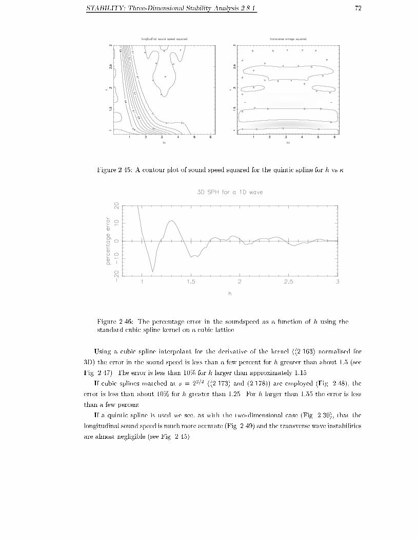
STABILITY: Three-Dimensional Stability Analysis 2.8.1 72
Figure 2.45: A contour plot of sound speed squared for the quintic spline for h vs �.
Figure 2.46: The percentage error in the soundspeed as a function of h using the
standard cubic spline kernel on a cubic lattice.
Using a cubic spline interpolant for the derivative of the kernel ((2.163) normalised for
3D) the error in the sound speed is less than a few percent for h greater than about 1:5 (see
Fig. 2.47). The error is less than 10% for h larger than approximately 1:15.
If cubic splines matched at s = 2
2=3
((2.173) and (2.178)) are employed (Fig. 2.48), the
error is less than about 10% for h greater than 1:25. For h larger than 1:55 the error is less
than a few percent.
If a quintic spline is used we see, as with the two-dimensional case (Fig. 2.30), that the
longitudinal sound speed is much more accurate (Fig. 2.49) and the transverse wave instabilities
are almost negligible (see Fig. 2.45).

STABILITY: Three-Dimensional Stability Analysis 2.8.1 73
Figure 2.47: The percentage error in the soundspeed as a function of h using the cubic
spline and spline interpolated derivative (matched at s
1
= 1) on a cubic lattice.
Figure 2.48: The percentage error in the soundspeed as a function of h using a cubic
spline and spline interpolated derivative (matched at s
1
= 2
2=3
) on a cubic lattice.

STABILITY: Three-Dimensional Stability Analysis 2.8.1 74
Figure 2.49: The percentage error in the soundspeed as a function of h using the
standard quintic spline kernel.

STABILITY: Three-Dimensional Stability Analysis 2.8.2 75
2.8.2 Body-Centred Cubic Lattice
Here we consider the properties of a body-centred cubic lattice. Such a lattice is \close packed"
and thus gives most neighbours within a volume for a given nearest neighbour distance. We
consider two lattices of particles using a similar approach to x 2.6.2
x
abc
= a�x+Xe
i�
; (2.185)
y
abc
= b�x+ Y e
i�
; (2.186)
z
abc
= c�x+ Ze
i�
; (2.187)
x
a
0
b
0
c
0
= (a
0
� 1=2)�x+Xe
i�
0
; (2.188)
y
a
0
b
0
c
0
= (b
0
� 1=2)�x+ Y e
i�
0
; (2.189)
z
a
0
b
0
c
0
= (c
0
� 1=2)�x+ Ze
i�
0
; (2.190)
where
� = �
x
a�x+ �
y
b�y + �
z
c�y � !t; (2.191)
�
0
= �
x
(a
0
� 1=2)�x+ �
y
(b
0
� 1=2)�y + �
z
(c
0
� 1=2)�y � !t: (2.192)
As in x 2.8.1 and x 2.6 we proceed to linearise the SPH momentum and continuity equations
and obtain a dispersion relation for waves parallel to the x-axis. We �nd the longitudinal
dispersion relation:
!
2
=
mc
2
�
0
2
8
<
:
X
i
X
j
X
k
(1� cos�i�x)
@
2
W
@x
2
+
X
i
0
X
j
0
X
k
0
(1� cos�(i
0
� 1=2)�x)
@
2
W
@x
2
9
=
;
�
�
mc
�
0
�
2
8
<
:
X
i
X
j
X
k
sin�i�x
@W
@x
+
X
i
0
X
j
0
X
k
0
sin�(i
0
� 1=2)�x
@W
@x
9
=
;
�
8
<
:
X
i
X
j
X
k
sin�i�x
@W
@x
+
X
i
0
X
j
0
X
k
0
sin�(i
0
� 1=2)�x
@W
@x
9
=
;
(2.193)
and a transverse wave solution (perturbations parallel to the y-axis, X = Z = 0):
!
2
=
mc
2
�
0
2
8
<
:
X
i
X
j
X
k
(1� cos�i�x)
@
2
W
@y
2
+
X
i
0
X
j
0
X
k
0
(1� cos�(i
0
� 1=2)�x)
@
2
W
@y
2
9
=
;
(2.194)
In these equations quantities present in summations over primed dummy indices are evaluated
on the second, displaced lattice. We wish to make a comparison with the results using the
cubic lattice such that there is approximately the same number of nearest neighbours for a
given smoothing length (ie- similar computational e�ort). Thus, we should choose a particle
spacing which gives the same number density. Since the body-centred cubic lattice consists of
two cubic lattices of spacing �x we require �x
3
= 2, giving,
�x = 2
1=3
: (2.195)

STABILITY: Three-Dimensional Stability Analysis 2.8.2 76
Figure 2.50: The percentage error in the soundspeed as a function of h using the
standard cubic spline on a body-centred cubic lattice.
Figure 2.51: The percentage error in the soundspeed as a function of h using the
cubic spline and spline interpolated derivative (matched at s
1
= 1) on a body-centred
cubic lattice.

STABILITY: Three-Dimensional Stability Analysis 2.8.2 77
Figure 2.52: The percentage error in the soundspeed as a function of h using the
modi�ed cubic spline and spline interpolated derivative matched at s
1
= 2
2=3
on a
body-centred cubic lattice.
Using the standard cubic spline (Fig. 2.50) the body-centred cubic results roughly resemble
the cubic lattice results. The smoothing length must be greater than 1:4 to ensure the errors
are less than 10%.
Using a cubic spline interpolant for the derivative of the kernel ((2.163) normalised for 3D)
the error in the sound speed is less than a few percent for h greater than about 1:35 (see
Fig. 2.51). The error is less than 10% for h larger than approximately 0:9.
If cubic splines matched at s = 2
2=3
((2.173) and (2.178)) are employed (Fig. 2.52), the
error is less than 10% for h greater than approximately 1:2. For h larger than about 1:4 the
error is less than a few percent.

STABILITY: Discussion 2.9 78
2.9 Discussion
2.9.1 Di�erent Methods for Dealing with Negative Stress
In the light of the results obtained for one-dimensional stability analysis we could suggest the
following methods for dealing with the instability induced by negative stress. Some of these
methods are considered in Chapt. 3 with regard to modelling MHD with SPH.
(i) Normalise the stress
By subtracting the most negative particle stress, we can force all the stresses to be positive
and use a method which ensures exact conservation of momentum. However, we have seen in
Fig. 2.9 that we must be careful with the particle spacing and smoothing length in order to
ensure stability. Using a smoother kernel improves these stability properties. It is also true
(Fig. 2.4) that an arti�cially large background stress can make the method very dispersive and
give an incorrect sound speed even for k = 0. Changing the stresses everywhere might also
complicate the implementation of boundary conditions in some problems.
(ii) \Mutate" the kernel
By using a correctly adjusted kernel (e.g. (2.71) with appropriate choices for B
n
) we
can obtain a realistic sound speed for a given background stress and smoothing length while
using an exactly momentum-conserving form. This is simple enough for a straightforward
adjustment of the gas pressure by a constant. In more complicated problems, where the
stresses experienced by the particle are not along the line between the interacting particles,
this is not as straightforward.
(iii) Normalise the stress and use mutated kernel to get sound speed correct
Having forced the stresses to be positive, we could then use an adjusted kernel to get the
correct sound speed for the arti�cially large background stresses. Method (ii) alone, however,
might be preferable for simplicity.
(iv) Use a stress di�erencing formulation
A formulation analogous to (2.41) could be used. This would simulate the propagation
of linear waves superbly (Fig. 2.21). Shocks, however, are not simulated as accurately. Since
di�erences are used to calculate the forces, negative stresses do not cause the method to become
unstable. In some problems, however, such a scheme might complicate the implementation of
boundary conditions.
2.9.2 What Should You Do?
Having considered the abilities of some methods to deal with negative stress, we can formulate
an approach for various problems.
If your problem involves no negative stresses use the \traditional" momentum-
conserving formulation. If you need to resolve linear waves particularly well and no strong
shocks will be present, use a di�erencing form.
If negative stresses are present but strong shocks absent, use a di�erencing formu-
lation.
If negative stresses are present and strong shocks are to occur but are pre-
dominantly hydrodynamical in nature use a hybrid method. The hydrodynamic pressure

STABILITY: Discussion 2.9.3 79
gradient may be implemented in a momentum-conserving form while other stresses appear
as di�erences. For example, in the case of magneto-hydrodynamics, the stress tensor may
be written as in (3.10). This implementation will be stable for any equation of state which
keeps the pressure positive. In many applications it is possible to isolate a part of the stress
which will always be positive. By implementing this force in a exactly momentum-conserving
form we improve the modelling of phenomena where momentum conservation is particularly
important, such as shocks. This approach is tested in x 3.4 with a variety of MHD shocks.
The successful implementation of a similar scheme elsewhere requires a sound understanding
of the signi�cance of the various forces in a given problem. Certainly there will be many prob-
lems where all forces are signi�cant, yet momentum conservation with regard to hydrodynamic
forces alone may be su�cient to resolve many types of strong shocks to high accuracy.
If negative stresses are present and strong shocks occur involving negative
stresses, use a mutating kernel if the negative stress is small. As we have seen, a mutat-
ing kernel can provide desirable properties but possibly only within an ever narrower band
of parameters for extreme negative stress. One could also normalise the stress and use the
exactly momentum-conserving form and pay the price of non-physical wave speeds if the re-
quired adjustment was extreme. A linear combination of the momentum-conserving form
using normalised stresses and a di�erencing formulation could be used. In regions not expe-
riencing shocks, or similar extreme circumstances where exact conservation of momentum is
particularly desirable, one would weight the di�erencing form most heavily. On shocks, one
would weight the stabilised momentum-conserving form most heavily. Thus, stability would be
guaranteed and linear waves propagated faithfully while conserving momentum exactly where
required. Of course, this requires that the algorithm employed be able to detect those regions
where momentum conservation is most necessary. Chapter 5 introduces a new switch for the
arti�cial viscosity which could be used for this purpose.
As was stated in the introduction, one of the attractive features of SPH is its robustness.
In dealing with instabilities we should seek a solution which is reliable and provides us with
the accuracy we require for a given problem. Hopefully, the approaches outlined above may
provide some ideas for formulating such methods for the various problems involving negative
stress to which SPH is applied.
2.9.3 Dealing with Instabilities in 2D and 3D SPH
As we have seen, two and three-dimensional SPH simulations can exhibit non-physical plane
wave solutions which can become unstable if low order spline approximations to the Gaussian
are employed. These instabilities cause particles initially stationary on a cubic or hexagonal
lattice to become slightly agitated. The resulting kinetic energy of the particles, however, is far
less than their thermal energy. As higher order spline approximations are used, this instability
becomes negligible. For a given h, a higher order spline will typically give a better estimate of
the sound speed. This would suggest that if it is essential that wave propagation be modelled
faithfully in a given simulation, a su�ciently high order spline interpolant should be used as a
kernel.
Kernels with compact support were originally introduced to reduce the number of neigh-
bouring particles which interact with a given particle. Typically, the higher the order of the

STABILITY: Conclusion 2.10 80
splines used, the less compact the constructed kernel will be and the more interacting neigh-
bours for a given h. However, in many cases, the use of a higher order spline may permit the
use of a smaller h, so the number of interacting neighbours may not increase by that much.
The results of x 2.7 and x 2.8 suggest the relatively poor performance of the low order
spline interpolated kernels may result from their derivatives being, e�ectively, even lower order
splines. Using separate cubic splines to interpolate both W and its gradients appears to give
more accurate numerical sound speeds. The issue of where to place the matching point in such
kernels is of interest also and may provide better results under some circumstances. Certainly,
using the one cubic spline with di�erent matching points did not improve the results (Fig. 2.38).
However, results obtained using separate splines for the kernel and derivatives matched at
equal-area and equal-volume points appear to have some promise. More testing is required to
determine how well such kernels perform in practice. There was not su�cient time for this to
be explored as part of this study.
Once the lattice is disordered, it would seem that the observed instabilities do not continue
to grow (see Fig. 2.28). However, as an extension to the work presented here, it would be
useful to understand how the numerical sound speed is a�ected by such disorder. It would be
relatively straightforward to do the linear stability analysis for a slightly disordered lattice. It
would most likely be the case that slightly larger smoothing lengths would be necessary for
accurate propagation of linear waves. The use of a pressure di�erencing formulation, however,
should remove such instabilities. It is trivial to show that a pressure di�erencing formulation
(such as (2.41)) does not support transverse waves. Linear transverse waves induce no �rst
order changes to the density, so the pressures at neighbouring particles are the same(to �rst
order), and particles experience no acceleration.
2.10 Conclusion
It is observed that the stability properties of SPH are improved by the use of kernels whose
Fourier transforms fall o� more rapidly. The instability �rst observed in exactly momentum-
conserving SPMHD (Phillips & Monaghan 1985) can be reproduced by a simple arti�cial
equation of state (2.14). There are many applications which involve an equation of state hav-
ing the e�ect of adjusting the background pressure acting between particles. Some examples
are MHD, incompressible SPH, elastic-plastic ow and problems where we model a uid ex-
periencing an external pressure. The pressure adjustment, when SPH is implemented in an
exactly momentum-conserving form, in uences the propagation of waves within the medium
but this in uence is reduced by the use of higher order spline interpolated kernels. Once the
stress acting between particles changes sign, however, a di�erent kernel must be used. It is pos-
sible to construct a kernel which varies with the stress acting between particles so as to ensure
stability and realistic wave propagation. However, for complicated equations of state in two
or three dimensions, this may not be feasible. Formulations of SPH which calculate the stress
gradients by taking di�erences between the stress at neighbouring particles are observed to
simulate the propagation of waves very well. The simulation of strong shocks, however, su�ers
since momentum is no longer conserved exactly. In many circumstances it may be best to split
the stress tensor into a component which is always positive and evaluate the remainder using
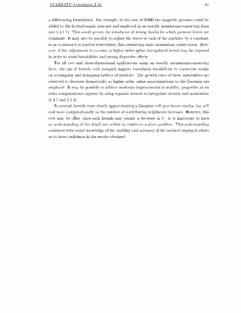
STABILITY: Conclusion 2.10 81
a di�erencing formulation. For example, in the case of MHD the magnetic pressure could be
added to the hydrodynamic pressure and employed in an exactly momentum-conserving form
(see x 3.1.1). This would permit the simulation of strong shocks for which pressure forces are
dominant. It may also be possible to adjust the stress at each of the particles by a constant,
so as to ensure it is positive everywhere, thus permitting exact momentum conservation. How-
ever, if the adjustment is extreme, a higher order spline interpolated kernel may be required
in order to avoid instabilities and strong dispersive e�ects.
For all two and three-dimensional applications using an exactly momentum-conserving
form, the use of kernels with compact support introduces instabilities in transverse modes
on rectangular and hexagonal lattices of particles. The growth rates of these instabilities are
observed to decrease dramatically as higher order spline approximations to the Gaussian are
employed. It may be possible to achieve moderate improvements in stability properties at no
extra computational expense by using separate kernels to interpolate density and momentum
(x 2.7 and x 2.8).
In general, kernels more closely approximating a Gaussian will give better results, but will
cost more computationally as the number of contributing neighbours increases. However, this
cost may be o�set since such kernels may permit a decrease in h. It is important to have
an understanding of the detail one wishes to resolve in a given problem. This understanding
combined with sound knowledge of the stability and accuracy of the method employed allows
us to have con�dence in the results obtained.

Chapter 3
Modelling MHD with SPH
\It must be a magnetic �elds thing..."
Someone discussing relationships at WholeFoods Restaurant
This chapter is intended to serve as an introduction to modelling magnetohydrodynamics
(MHD) with SPH. Some technical di�culties are discussed in detail and methods are suggested
for dealing with them. Some of these problems have been pointed out by previous authors
(Meglicki 1995, Phillips & Monaghan 1985), however, not many practical solutions have been
suggested. There are several approaches which can be taken when trying to develop a particle
MHD method. One could develop a hybrid particle-grid method where the magnetic �eld is
solved on a grid (possibly using an already established and tested code) while the particles
are used to evaluate the hydrodynamical forces (Leboeuf, Tajima & Dawson 1979, Brackbill
1991). Another approach is to take all of the equations of MHD and reformulate the particle
method so as to solve them without a grid. We will consider this latter approach with regard to
SPH in order to derive and test implementations of smoothed particle magnetohydrodynamics
(SPMHD).
The inclusion of magnetic forces into SPH was �rst considered by Gingold & Monaghan
(1977) in connection with modelling magnetic �elds in polytropes. Since then, many authors
have considered the modelling of MHD with SPH and have simulated a wide range of problems:
the collapse of isothermal magnetised clouds (Phillips 1983, Phillips & Monaghan 1985, Phillips
1986a, Phillips 1986b), blast waves in a magnetic medium (Stellingwerf 1990) and the gravi-
tational collapse of a magnetised vortex (Meglicki, Wickramasinghe & Dewar 1995), to name
a few.
Many authors have discussed some of the technical problems encountered when modelling
MHD with SPH. It was Phillips & Monaghan (1985) who �rst commented that SPH particles
appeared to be unstable to negative stress. A later report (Stellingwerf & Peterkin 1990) on
the incorporation of MHD into an existing SPH code also noted this problem. Meglicki et al.
(1995) and Meglicki (1995) used an expression based on j �B (3.12) to avoid the instability.
The nature of this instability (and others) is investigated in detail in Chapt. 2. We will use
the results of this analysis (see x 2.9.1) to avoid instabilities resulting from negative stress.
82
MHD: The Various Approaches 3.1 83
A second technical problem which all MHD codes must address was pointed out by Brackbill
& Barnes (1980). Instabilities were observed to occur if the magnetic �eld was not kept
solenoidal and a conservative form of the momentum equation was used. The problem appears
to result from the magnetic force having a component along the �eld lines if the �eld is
non-solenoidal. In x 3.1.2 several approaches whereby this might be reduced with SPMHD
are discussed. The easiest of these to implement involves the introduction of an arti�cial
dissipation to ensure the �eld remains ordered at the resolution length of the simulation. Of
course, the instability can also be avoided by using a non-conservative form of SPMHD.
This chapter explores the various approaches that can be used to incorporate MHD into
SPH. The two main problems outlined above are considered in detail and various test cases
are considered to show the relative merits of the suggested solutions.
3.1 The Various Approaches
Let us consider the basic equations of MHD. The uid equations are the continuity
D�
Dt
+ �r � v = 0 (3.1)
and momentum equations
Dv
Dt
= �
1
�
rp+
1
�
j�B (3.2)
where
D
Dt
is the comoving time derivative and
j =
1
�
r�B; (3.3)
where � is the permeability (in general we will use S.I. units). The magnetic �eld B is evolved
according to
@B
@t
= r� (v �B) + �r
2
B; (3.4)
where � is the resistivity.
3.1.1 Modelling the Lorentz Force
Let us concentrate on the Lorentz force term for a moment. Substituting for j we have
j�B =
1
�
(r�B)�B: (3.5)
This, in turn, can be expressed as the gradient of a symmetric magnetic stress tensor
(j�B)
i
=
@M
ij
@x
j
(3.6)
where
M
ij
=
1
�
0
B
B
@
B
2
x
�
1
2
B
2
B
x
B
y
B
x
B
z
B
y
B
x
B
2
y
�
1
2
B
2
B
y
B
z
B
z
B
x
B
z
B
y
B
2
z
�
1
2
B
2
1
C
C
A
(3.7)
=
1
�
�
B
i
B
j
�
1
2
B
2
�
ij
�
: (3.8)

MHD: The Various Approaches 3.1.2 84
It is straightforward to write an SPH approximation of the gradient ofM
ij
which is antisym-
metric and thus conserves linear momentum exactly.
1
�
�
@M
ij
@x
i
�
a
=
X
b
m
b
��
M
ij
�
2
�
a
+
�
M
ij
�
2
�
b
�
r
a;j
W
ab
: (3.9)
Here, r
a;j
W
ab
denotes the j-th component of the gradient of W
ab
with respect to r
a
. How-
ever, this formulation is observed to be unstable for some circumstances where the magnetic
stress and gas pressure are comparable in magnitude. The reason is that the stress between
particles can become negative and SPH particles su�er a numerical instability under negative
stresses (see Chapt. 2). It is possible to remove this instability and retain exact conservation
of momentum by normalising the tensor M
ij
. This is done by subtracting a constant from
the components of M
ij
such that all components are negative.
In (3.8) the magnetic stress tensor is shown to be the sum of a magnetic pressure and
other stress terms. Since the magnetic pressure is always positive, it is possible to estimate
its gradient using a momentum-conserving form. We will, for the most part, use a split tensor
formulation:
1
�
�
@M
ij
@x
i
�
a
= �
1
2�
X
b
m
b
�
B
2
a
�
2
a
+
B
2
b
�
2
b
�
r
a;i
W
ab
+
1
�
X
b
m
b
(B
i
B
j
)
b
� (B
i
B
j
)
a
�
a
�
b
r
a;j
W
ab
: (3.10)
It can be shown (see x 2.3.3.1, Morris (1994) and Morris (1996b)) that for certain choices of
smoothing length and spline kernel, the \over pressure" resulting from the magnetic pressure
can lead to long wave numerical instabilities. These instabilities become negligible as smoother
splines are employed. Another possibility is to use a straightforward SPH approximation of
the curl operator
1
��
(r�B)�B
=
1
��
2
a
"
X
b
m
b
B
ab
�r
a
W
ab
#
�B
a
(3.11)
=
1
��
2
a
X
b
m
b
f(B
ab
�B
a
)r
a
W
ab
� (B
a
� r
a
W
ab
)B
ab
g : (3.12)
This form was used in Meglicki et al. (1995) and Meglicki (1995) and has some advantages.
The SPH estimate of the magnetic force is guaranteed to be perpendicular to the magnetic
�eld, however, momentum conservation can be a problem (see x 3.4.2).
3.1.2 Updating the Magnetic Field
There are several issues to consider when deciding how the magnetic �eld should be updated.
Implicit in the derivation of the evolution equation for B (3.4) is the requirement that the �eld
be divergence free:
r �B = 0: (3.13)
An initially solenoidal �eld will remain divergence free if evolved using (3.4). When the �eld
is evolved numerically, it is important that this property be preserved. Numerical instabilities

MHD: The Various Approaches 3.1.2.1 85
may result if the divergence of B is substantially non-zero and a conservative formulation of
the momentum equation is employed (Brackbill & Barnes 1980). The severity of this problem
is brie y investigated in x 3.5
We will be considering ideal MHD where the conduction may be considered in�nite and
the resistivity � zero:
@B
@t
= r� (v �B) : (3.14)
This limit is also referred to as \ ux freezing" since (3.14) implies that �eld lines are \tied"
to the uid.
3.1.2.1 Evolving Particle Fields
The most straightforward approach is to assign the magnetic �eld to each particle and evolve
the �eld according to an SPH version of (3.14). There are several ways in which this can be
done.
Using
d
dt
�
B
�
�
=
�
B
�
2
� r
�
�v �
v
�
2
(B � r�) (3.15)
we obtain
d
dt
�
B
�
�
a
= �
1
�
2
a
X
b
m
b
v
ab
(B
a
� r
a
W
ab
) : (3.16)
In this case, part of the variation in B is accounted for by variations in density. This means,
for example, that we expect the evolution of magnetic �eld to be modelled very well for
perpendicular shocks. However (see x 3.4.1) the primary issue in resolving MHD shocks appears
to be conservation of momentum. In the test cases presented here, there did not appear to be
any substantial di�erence between the possible evolution equations for B.
Writing
dB
dt
= �B (r � v) + (B � r)v; (3.17)
leads to
dB
a
dt
=
1
�
a
X
b
m
b
fB
a
(v
ab
� r
a
W
ab
)� v
ab
(B
a
� r
a
W
ab
)g : (3.18)
Here, these terms model squeezing and shearing of �eld lines respectively.
These equations for updating the magnetic �eld do not guarantee the �eld will remain
solenoidal. Tests (see x 3.6.2) show that ows which lead to the �eld being \wound up" cause
the magnetic �eld to become disordered and non-solenoidal. In most numerical methods there
is some numerical dissipation which would keep the �eld smooth as it is wound up on scales
smaller than the resolution length. Since SPH is a Lagrangian method, the particles carry the
�eld with them, and their motion can lead to the �eld being wound up beyond the resolution
of the method. Thus, some form of dissipation should be introduced to keep the magnetic �eld
smooth over distances corresponding to the resolution of the method. This arti�cial dissipation
could be introduced as some small resistivity, larger than that of the real system:
�
dB
dt
�
diss
= �r
2
B =
X
b
m
b
(�
a
+ �
b
) (B
a
�B
b
) r
ab
� r
a
W
ab
�
b
(r
2
ab
+ 0:01h
2
)
: (3.19)
This term is simply added onto the evolution equation for B. The SPH form of r
2
has already
been discussed for the case of thermal conduction (1.51). The above summation can be shown

MHD: The Various Approaches 3.1.2.1 86
to reduce to �r
2
B and is less subject to interpolation errors than using a summation involving
second derivatives of the kernel.
However, it may be better to use an arti�cial dissipation based on the arti�cial viscosity
(1.46) with magnetic �eld replacing velocity:
�
dB
dt
�
diss
=
X
b
m
b
�
B
h(�v
A
)
ab
(B
a
�B
b
) � r
ab
��
ab
(r
2
ab
+ 0:01h
2
)
r
a
W
ab
; (3.20)
where �
B
is a nondimensional coe�cient and v
A
=
p
B
2
=�� is the Alfv�en speed. A bar over
a quantity represents an average between particles. The arti�cial viscosity (x 1.1.5) in SPH is
used to keep the velocity smooth through shocks and is intended to be largest in regions of
high compression (r � v < 0). The SPMHD expression for r �B (c.f. (1.12)) is
r �B
a
=
1
�
a
X
b
m
b
(B
b
�B
a
) � r
a
W (r� r
b
; h): (3.21)
The form of the arti�cial dissipation (3.20) favours the cancellation of magnetic �eld where
(B
a
�B
b
) �r
ab
6= 0. It is terms such as this which contribute to the local estimate of r�B, since
r
a
W
ab
can be written in the form r
ab
F
ab
. Although not equivalent to r�B being substantially
non-zero the individual pairwise contributions to r �B will tend to be large in regions of high
divergence.
The typical astrophysical applications of SPMHD will involve high magnetic Reynolds
numbers
R
m
=
V L
�
; (3.22)
where V and L are typical velocity and length scales. The form of dissipation (3.20) is intended
to smooth the �eld on lengthscales of order h without leading to larger scale dissipative e�ects.
We need to be sure the arti�cial dissipation does not introduce excessive �nite conduction
e�ects into the simulation. Taking the e�ective Reynolds number resulting from the arti�cial
viscosity (Chapt. 5) we can, by analogy, see that the arti�cial dissipation gives a magnetic
Reynolds number of
R
m
=
8V L
�
B
v
A
h
: (3.23)
Here B and L denote the typical magnetic �eld and length scale respectively. It is important
to check that R
m
due to the arti�cial dissipation is su�ciently large in a given simulation. If it
isn't, it may be possible to increase the resolution or use a switch similar to that developed for
use with the arti�cial viscosity (see Chapt. 5 and Morris & Monaghan (1996)). Using a source
term which depended on (r�B)
a
dissipation would be present where the �eld is non-solenoidal
and relatively small elsewhere. There should be some dissipation present everywhere to help
keep the magnetic �eld smooth. The role of dissipation in some test cases is considered in
x 3.6.2.
The arti�cial dissipation (3.20) leads to heating of the gas (by conservation of energy). The
heating term can be found by considering the rate of change of magnetic energy due to this
dissipation term. If E
M
denotes the total magnetic energy, then
E
M
=
X
a
m
a
�
a
B
2
a
2�
; (3.24)

MHD: The Various Approaches 3.1.2.2 87
and
dE
M
dt
=
X
a
m
a
2�
�
�
a
d
dt
B
2
a
�B
2
a
d�
a
dt
�
=�
2
a
(3.25)
=
X
a
m
a
2�
�
�
a
B
a
�
dB
a
dt
�B
2
a
d�
a
dt
�
=�
2
a
(3.26)
Since we are only interested in changes in magnetic energy due to the arti�cial dissipation
term we write:
�
dE
M
dt
�
diss
=
X
a
m
a
1
��
a
B
a
�
�
dB
a
dt
�
diss
(3.27)
=
X
a
m
a
�
B
a
�
a
�
X
b
m
b
�
B
h(�v
A
)
ab
B
ab
� r
ab
��
ab
r
2
ab
r
a
W
ab
(3.28)
=
X
a
X
b
m
a
m
b
1
�
�
B
h(�v
A
)
ab
B
ab
� r
ab
��
ab
r
2
ab
�
B
a
�
a
�
� r
a
W
ab
(3.29)
=
X
a
X
b
m
a
m
b
1
�
�
B
h(�v
A
)
ab
B
ab
� r
ab
��
ab
r
2
ab
�
�
B
b
�
b
�
� r
a
W
ab
(3.30)
=
X
a
m
a
1
2
X
b
m
b
�
�
B
h(�v
A
)
ab
B
ab
� r
ab
��
ab
r
2
ab
�
B
a
�
a
�
B
b
�
b
�
� r
a
W
ab
: (3.31)
So, we make the association
�
du
dt
�
diss
=
1
2
X
b
m
b
�
�
B
h(�v
A
)
ab
B
ab
� r
ab
��
ab
r
2
ab
�
B
a
�
a
�
B
b
�
b
�
� r
a
W
ab
(3.32)
to conserve total energy.
3.1.2.2 Interpolating Particle Fluxes
An interesting alternative is to attempt to calculate the magnetic �eld using a method similar
to that with which density is obtained. The basic idea is to assign a constant magnetic ux
to each particle and obtain the magnetic �eld at a point by summation over neighbouring
particles. Particles are connected by elements of ux tubes to form �eld lines as depicted in
Fig. 3.1. We de�ne �
i
to be the ux threading the i-th ux tube. The vector �x
a
is the
displacement from particle a to the next particle in the tube while �x
0
a
is the displacement
from the previous particle to a. Flux has the units of magnetic �eld by unit area, while the
kernel,W , is measured in units of inverse volume. If we sum over the product of ux threading
an element, the length of each element of ux and the kernel, we recover the contribution to
the magnetic �eld (a more detailed argument appears in x A.2). The contribution from particle
b in ux tube i to the magnetic �eld at a point a is then
�
i
�x
0
b
+�x
b
2
W
ab
(3.33)
Thus, we can write the magnetic �eld at particle a
B
a
=
X
b
�
i(b)
�x
0
b
+�x
b
2
W
ab
(3.34)

MHD: The Various Approaches 3.1.2.2 88
a
ax
x
∆
a∆
Figure 3.1: Field can be calculated at a point by summing over elements of ux.
where i(b) denotes the index of the ux tube to which particle b belongs. In practice, linked lists
could be used to provide pointers from a given particle to the next particle in either direction
along the ux tube. As the particles move, the elements are carried with them leading to the
ux being \frozen" into the uid and the �eld is kept divergence free.
However, there are several technical problems with this approach. If particles are stretched
out along �eld lines by the uid motion, they may become so distant that other particles
may pass freely through the ux tube. The problem is similar to that in pure hydrodynamics
where (if h is not varied in space and time) particles can lose contact with each other in rare�ed
regions. The problem may be alleviated by introducing extra particles along a ux tube which
have no mass (so they do not appear elsewhere in the SPH equations) but contribute to the
magnetic �eld calculation by (3.34). These particles would be moved with an interpolated
velocity since they do not enter into the momentum equation
v
0
a
=
X
b
m
b
�
b
v
b
W
ab
: (3.35)
This can, however, lead to huge numbers of particles being introduced into the simulation and
a drastic increase in computational e�ort. Another serious problem is that twisting of the �eld
lines can lead to �eld lines passing through each other or becoming tangled. Normally (see
x 3.1.2.1) numerical MHD schemes will have numerical dissipation present which will cause
�eld lines to reconnect as they cross. This formulation of SPMHD has no such dissipation
and thus has di�culty modelling the ow as it is twisted up and becomes more complicated.
In x 3.1.2.1 we discussed the role of an arti�cial conductivity in such situations, however,
there is no clear way to implement this when the �eld is explicitly tied to the particles, since
conductivity permits the �eld to pull through the uid. A solution to this problem would be
to model the uid using two components. The �eld lines would be tied to massless particles.
These particles could have a drag acting between them and the real particles which keeps
them moving with the uid but still permits the uid to ow across �eld lines. If �eld lines
cross they can be reconnected by making appropriate changes to the data structures linking
particles along the ux tubes. There was not time to explore the potential of this method in
MHD: The Various Approaches 3.1.2.3 89
full during this study. While it would be impractical in a simulation involving the twisting up
of �eld, it could be quite useful in quasi-magnetostatic situations.
3.1.2.3 Other Possibilities
There are other methods for evolving the �eld which were not investigated by this study. It
is possible to evolve the �eld using Clebsch variables (Roberts 1967). This approach involves
writing the magnetic �eld as a cross product of the gradients of two scalars:
B = rF �rG (3.36)
where dF=dt = 0 and dG=dt = 0. However, Phillips (1983) found that in simulations involving
substantially non-uniform density, the method was less accurate than evolving the �eld directly.
It is also possible to use the vector potential A
B = r�A; (3.37)
which may be evolved using
@A
@t
= v � (r�A) +r�; (3.38)
where � is an arbitrary scalar function. However, this will require that the curl of A be
taken to obtain B so the forces may be calculated. This will, e�ectively, involve taking second
derivatives of the vector potential to obtain the magnetic force and may lead to larger errors
in the estimation of the Lorentz force.
3.2 The Arti�cial Viscosity
As with normal hydrodynamic SPH an arti�cial viscosity is used to provide the necessary
dissipation at a shock front (see x 1.1.5). In order for the arti�cial viscosity to be e�ective at
shock fronts which are dominated by magnetic forces (v
A
� c
s
, where v
A
=
p
B
2
=�� is the
Alfv�en speed) the following should be used:
�
ab
=
(
��max(�c;�v
A
)�
ab
+��
ab
2
��
ab
; if v
ab
� r
ab
< 0;
0; otherwise,
(3.39)
While this form of viscosity is very successful when employed with perpendicular shocks
(x 3.4.1) it is not su�cient when oblique shocks are modelled (x 3.4.2). The problem is
that the standard form of SPH arti�cial viscosity (3.39) was designed to dampen compressive
shocks, while oblique shocks can involve large shearing forces. To provide a suitable form of
dissipation, the following form of shear viscosity was used:
dv
a
dt
=
X
b
m
b
�
s
max (�c; �v
A
)h
��
ab
v
ab
(r
ab
� r
a
W
ab
)
r
2
ab
+ �
2
: (3.40)
This was obtained by considering the SPH equation for an arti�cial conductivity (1.52) and re-
placing u
ab
with v
ab
and (q
a
+q
b
) with �
s
max (�c; �v
A
)h. This form of viscosity, by conservation
of total energy, introduces a new source term in the internal energy equation:
du
a
dt
= �
X
b
m
b
�
s
max (�c; �v
A
) h
��
1
2
v
2
ab
r
ab
� r
a
W
ab
r
2
ab
+ �
2
: (3.41)

MHD: The Consistency of the Equations 3.3 90
In general, it is undesirable to have large amounts of viscosity present throughout the compu-
tational domain. Ideally, the arti�cial viscosities are only introduced at the shock front. This
can be achieved by an approach similar to that explored in Chapt. 5. The viscosity coe�cients
� and �
s
can be evolved according to a di�erential equation which introduces viscosity where
it is needed.
3.3 The Consistency of the Equations
Ideally we wish the total energy of our numerical simulation to be conserved exactly. Already,
the consistency of the momentum equation for pressure and that used for internal energy has
been demonstrated ((1.40) and (1.44)). Source terms for the internal energy corresponding to
the arti�cial viscosities ((1.49) and (3.41)) and the arti�cial dissipation (3.32) have also been
discussed. Here we will consider the relationship between the contribution to kinetic energy
from magnetic forces and the magnetic energy density in the absence of dissipation.
If the exactly momentum-conserving form (3.9) is used, we �nd the total kinetic energy
E
k
=
X
a
1
2
m
a
(v
a
)
2
(3.42)
evolves according to (see x A.1)
dE
k
dt
=
X
a
X
b
m
a
m
b
�
v
ab
�B
a
�
2
a
(B
a
� r
a
W
ab
)
�
X
a
X
b
m
a
m
b
2�
1
2
�
B
2
a
�
2
a
+
B
2
b
�
2
b
�
v
ab
� r
a
W
ab
: (3.43)
When using the split tensor formulation (3.10), we �nd
dE
k
dt
= �
X
a
X
b
m
a
m
b
�
(v
a
+ v
b
) �B
a
�
a
�
b
(B
a
� rW
ab
)
�
X
a
X
b
m
a
m
b
2�
1
2
�
B
2
a
�
2
a
+
B
2
b
�
2
b
�
v
ab
� r
a
W
ab
: (3.44)
The change in total magnetic energy,
E
M
=
X
a
m
a
2�
B
2
a
�
a
(3.45)
due to the magnetic evolution (3.18) is given by:
dE
M
dt
= �
X
a
X
b
m
a
m
b
�
v
ab
�B
a
�
2
a
B
a
� r
a
W
ab
+
X
a
X
b
m
a
m
b
2�
1
2
�
B
2
a
�
2
a
+
B
2
b
�
2
b
�
v
ab
� r
a
W
ab
: (3.46)
The same result is obtained if (3.16) is used to evolve the magnetic �eld.
Comparing (3.46) and (3.43), it is clear that using the exactly momentum-conserving for-
mulation (3.9) with either (3.18) or (3.16) is consistent and results in exact conservation of
total energy to within time integration error. However, in practice, the stress tensor is nor-
malised to ensure stability (see x 3.1.1). Using the normalised stress in the magnetic evolution
MHD: Modelling MHD Shocks 3.4 91
equations is inappropriate, since these equations do not only involve gradients of the magnetic
�eld. Thus, the normalisation would lead to non-physical evolution of magnetic �eld.
When the split tensor formulation is used (3.10) we see that the second terms in (3.44)
and (3.46) are identical. Since these terms correspond to the magnetic pressure we conclude
that total energy is conserved exactly with respect to magnetic pressure forces but not the
magnetic shear forces.
It can be shown (Meglicki 1995) that using (3.12) and (3.18) is consistent to within order
h
2
. In general we expect the the solutions to be consistent to at least h
2
since this is the order
of accuracy of the SPH approximations to the original di�erential equations.
3.4 Modelling MHD Shocks
In many astrophysical applications, shocks can develop as the simulation progresses. This
section investigates the relative merits of various approaches to SPMHD when modelling a
range of MHD shocks. We will consider four methods:
Method 1 : Evolve the �eld with (3.18) and use (3.12).
Method 2 : Use (3.18) to evolve the magnetic �eld and use (3.10).
Method 3 : Use (3.16) to evolve the �eld and use (3.10).
Method 4 : Evolve the �eld with (3.18) and use (3.9) with a normalised stress tensor.
We expect that Method 1 will be best at modelling propagation of linear waves since formu-
lations employing di�erences have better stability properties (see x 2.3.3.6). However, since it
does not conserve momentum exactly, it will not simulate strong shocks nearly as well.
Method 2 may have some di�culty modelling linear waves realistically for strong magnetic
�elds if a low order cubic spline is used (see x 2.3.3.1). Such problems should be reduced when
higher order splines, such as the quartic (Fig. 2.10) or quintic spline interpolant kernels are
used. The advantage of Method 2 over Method 1 is that total momentum and total energy
are conserved with respect to magnetic pressure forces (see x 3.3).
Method 4 allows linear momentum to be conserved exactly but total energy is only approx-
imately conserved with respect to magnetic forces (see x 3.3). In some cases renormalising the
stress tensor may lead to the \background stress" being approximately zero (this corresponds
to < � 0 in Chapt. 2 or using the gauge pressure in x 5.2.3). In this case the accuracy of the
SPH interpolation can be improved (see x D). In general, however, the renormalisation may
lead to quite large \background stresses" in some regions and, thus, quite unphysical wave
speeds for lower order kernels.
Method 3 is included to see if evolving B=� has any real advantage over evolving B.
In all of the following sections the shocks were modelled using periodic boundary conditions
in the y-direction (Fig. 3.2). The particles had a pre-shock spacing of 1 and h = 1:2 was used
throughout. The standard SPH viscosity (x 1.1.5) was used with � = 1 and � = 2. Where
indicated, the arti�cial shear viscosity (x 3.2) was also used. Initially particles were assigned
quantities appropriate to the pre- and post-shock conditions. Particles were continuously fed
into the region from the right with the pre-shock quantities prescribed in a \bu�er zone". A
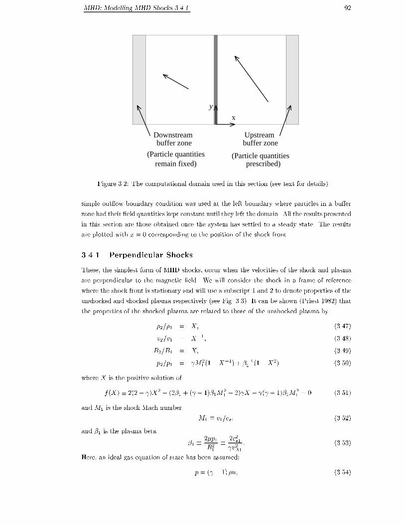
MHD: Modelling MHD Shocks 3.4.1 92
buffer zone
(Particle quantitiesremain fixed)
buffer zoneUpstream
(Particle quantitiesprescribed)
Downstream
x
y
Figure 3.2: The computational domain used in this section (see text for details).
simple out ow boundary condition was used at the left boundary where particles in a bu�er
zone had their �eld quantities kept constant until they left the domain. All the results presented
in this section are those obtained once the system has settled to a steady state. The results
are plotted with x = 0 corresponding to the position of the shock front.
3.4.1 Perpendicular Shocks
These, the simplest form of MHD shocks, occur when the velocities of the shock and plasma
are perpendicular to the magnetic �eld. We will consider the shock in a frame of reference
where the shock front is stationary and will use a subscript 1 and 2 to denote properties of the
unshocked and shocked plasma respectively (see Fig. 3.3). It can be shown (Priest 1982) that
the properties of the shocked plasma are related to those of the unshocked plasma by
�
2
=�
1
= X; (3.47)
v
2
=v
1
= X
�1
; (3.48)
B
2
=B
1
= X; (3.49)
p
2
=p
1
= M
2
1
(1�X
�1
) + �
�1
1
(1�X
2
) (3.50)
where X is the positive solution of
f(X) � 2(2� )X
2
+ (2�
1
+ ( � 1)�
1
M
2
1
+ 2) X � ( + 1)�
1
M
2
1
= 0 (3.51)
and M
1
is the shock Mach number
M
1
� v
1
=c
s1
(3.52)
and �
1
is the plasma beta
�
1
�
2�p
1
B
2
1
�
2c
2
s1
v
2
A1
: (3.53)
Here, an ideal gas equation of state has been assumed:
p = ( � 1) �u; (3.54)

MHD: Modelling MHD Shocks 3.4.1 93
v2
ρ2
p2
B2
v1
ρ1
p1
B1
Figure 3.3: Depiction of a perpendicular shock. Solid lines represent the �eld lines
while dashed lines represent the velocity.
where u is the internal energy of the gas and the ratio of speci�c heats. Let us initially con-
pre-shock post-shock
� 1 2.9436
v 5 1.6986
B 1 2.9436
p 1 13.6746
Table 3.1: The pre- and post-shock states for a weak perpendicular shock using
� = 1:0 and = 5=3.
Figure 3.4: Weak perpendicular shock using Method 1.
sider a relatively weak perpendicular shock (see Table 3.1). We expect that exact conservation
of momentum is not so important for a weak shock and, accordingly, Method 1 works quite

MHD: Modelling MHD Shocks 3.4.2 94
Figure 3.5: Weak perpendicular shock using Method 2.
well, with only a slight error in the post-shock B
y
(Fig. 3.4). The post-shock states obtained
with Method 2 (Fig. 3.5) are indistinguishable from the exact values.
pre-shock post-shock
� 1 3.4177
v 50 14.6294
B 1 3.4177
p 1 1235.4718
Table 3.2: The pre- and post-shock states for a strong perpendicular shock using
� = 0:01 and = 5=3.
Figure 3.6: Strong perpendicular shock using Method 1.
Let us now consider a stronger perpendicular shock (see Table 3.2). Method 1 (Fig. 3.6)
displays errors of order 10% in the post-shock B
y
. Once again results obtained using Method 2
are indistinguishable from the exact values away from the shock front.

MHD: Modelling MHD Shocks 3.4.2.1 95
Figure 3.7: Strong perpendicular shock using Method 2.
3.4.2 Oblique Shocks
A more general form of MHD shock is that where the magnetic �eld has components both
parallel and perpendicular to the shock front. Once again we consider the plasma in a frame
co-moving with the shock front and denote the unshocked and shocked plasma quantities by
subscripted 1 and 2 respectively. The analysis is simpli�ed to some extent, by considering a
frame moving parallel to the shock front such that
v
1y
= v
1x
B
1y
B
1x
: (3.55)
This results in the plasma velocity being parallel to the magnetic �eld on both sides of the
shock front. It can then be shown (Priest 1982) that
�
2
=�
1
= X; (3.56)
v
2x
=v
1x
= X
�1
; (3.57)
v
2y
=v
1y
=
v
2
1
� v
2
A1
v
2
1
� xv
2
A1
; (3.58)
B
2x
=B
1x
= 1; (3.59)
B
2y
=B
1y
=
(v
2
1
� v
2
A1
)X
v
2
1
�Xv
2
A1
; (3.60)
p
2
=p
1
= X +
( � 1)Xv
2
1
2c
2
s1
�
1�
v
2
2
v
2
1
�
(3.61)
where X is a solution of
(v
2
1
�Xv
2
A1
)
2
fXc
2
s1
+
1
2
v
2
1
cos
2
�(X( � 1)� ( + 1))g
+
1
2
v
2
A1
v
2
1
sin
2
�
�Xf( +X(2� ))v
2
1
�Xv
2
A1
(( + 1)�X( � 1))g = 0 (3.62)
and � is the inclination of the upstream magnetic �eld to the shock normal (see Fig. 3.8).
A full derivation of the properties of oblique shocks is presented in Bazer & Ericson (1959)
and Je�rey & Taniuti (1964) and a fairly detailed summary can be found in Priest (1982).
Here we will consider two basic types of oblique shocks.

MHD: Modelling MHD Shocks 3.4.2.1 96
p2
ρ1
p1
2B
2v
ρ
1
1
v
1B
2
x
y
θ
Figure 3.8: Depiction of an oblique shock. Solid lines represent the �eld lines while
dashed lines represent the velocity.
3.4.2.1 Slow Shocks
Slow shocks are compressive (X > 1) with
B
2
< B
1
(3.63)
where B
1
= jB
1
j an B
2
= jB
2
j. Since the component of magnetic �eld perpendicular to the
shock front remains unchanged, the magnetic �eld (and hence the velocity �eld in the frame
of reference chosen) is refracted towards the shock normal.
Slow shocks have a speed faster than the pre-shock slow magnetoacoustic speed, but slower
than the fast magnetoacoustic speed. Thus it is possible for information to propagate ahead of
the shock front into the pre-shock region. As a result, errors in the simulated jump conditions
can lead to discrepancies in the pre-shock conditions.
pre-shock post-shock
� 1 2.6667
u 3.53553 1.3258
v 3.53553 0.0
B
x
0.7071 0.7071
B
y
0.7071 0.0
p 1 15.0625
Table 3.3: Weak switch o� shock pre- and post- shock states with � = 0:04 and
= 5=3.
We will consider \switch o�" shocks, a limiting case of slow shocks, where the �nal velocity
and magnetic �eld are normal to the shock front. We will �rst consider a relatively weak switch-
o� shock with states given in Table 3.3. This shock does not involve particularly large shear

MHD: Modelling MHD Shocks 3.4.2.1 97
Figure 3.9: Weak \switch-o�" shock using Method 2 and no extra shear viscosity
(�
s
= 0).
Figure 3.10: Weak \switch-o�" shock using Method 2 with �
s
= 1=2.
Figure 3.11: Weak \switch-o�" shock using Method 2 with �
s
= 1.

MHD: Modelling MHD Shocks 3.4.2.2 98
Figure 3.12: Weak \switch-o�" shock using Method 1.
stresses across the interface. This particular example allows us to compare the performance
of the various methods when weak shear forces are present. The \switch on" shock of the
following section is a more extreme test.
Even though the shear stresses are rather weak, if this problem is modelled without the
extra arti�cial shear viscosity (3.40), the uid is observed to oscillate quite strongly downstream
of the shock front (Fig. 3.9). The standard arti�cial viscosity alone is clearly not su�cient
to provide the necessary dissipation at a shock front where shear forces are important. Using
�
s
= 1=2 greatly reduces (Fig. 3.10), while �
s
= 1 almost entirely removes (Fig. 3.11), these
oscillations. All results in this section presented after Fig. 3.11 use �
s
= 1.
The largest errors appear to be in the pre-shock quantities. Being a slow-shock, the shock
speed is actually slower than the fast magnetoacoustic wave speed. Thus, errors at the shock
front can be propagated upstream. The upstream results using Method 2 improve with the
introduction of the shear viscosity and are substantially less than those present when Method 1
is used (Fig. 3.12). It is to be expected that some smoothing of the interface will improve the
accuracy of the SPH interpolation and thus improve the results. It is also possible that the
improvement in pre-shock quantities with the introduction of the arti�cial shear viscosity is in
part to the fact that the viscosity conserves linear momentum exactly. The greater the role of
the viscosity, the better the level of conservation. The main purpose of the viscosity, however,
is to prevent excessive transverse oscillation of the post shock material by converting kinetic
energy into internal energy.
The states for a stronger switch-o� shock appear in Table 3.4. As expected, the results
obtained using Method 1 (Fig. 3.13) show substantial errors as shear forces become more
important. Method 2 (Fig. 3.14) has errors of practically the same magnitude as it did for
the weak switch-o� case (Fig. 3.11). Using Method 3 does not appear to have any measurable
e�ect on the results (Fig. 3.15). Method 4 also exhibits very similar errors in the upstream
quantities (Fig. 3.16), suggesting that these errors are the result of total energy not being
conserved across the shock front.

MHD: Modelling MHD Shocks 3.4.2.2 99
pre-shock post-shock
� 1 3.1008
u 35.3553 11.4020
v 35.3553 0.0
B
x
0.7071 0.7071
B
y
0.7071 0.0
p 1 1472.8788
Table 3.4: Strong switch o� shock pre- and post- shock states with � = 0:0004 and
= 5=3.
Figure 3.13: Strong \switch-o�" shock using Method 1
Figure 3.14: Strong \switch-o�" shock using Method 2.

MHD: Modelling MHD Shocks 3.4.2.2 100
Figure 3.15: Strong \switch-o�" shock using Method 3.
Figure 3.16: Strong \switch-o�" shock using Method 4.

MHD: The E�ect of Non-Zero Divergence 3.5 101
3.4.2.2 Fast Shocks
Fast shocks are also compressive (X > 1) but result in
B
2
> B
1
: (3.64)
Since the component of magnetic �eld perpendicular to the shock front remains unchanged,
the magnetic �eld (and hence the velocity �eld in the frame of reference chosen) is refracted
away from the shock normal.
pre-shock post-shock
� 1 3.3632
u 91.6964039 27.2638
v 0 27.2638
B
x
1 1
B
y
0 1
p 1 4659.2304
Table 3.5: Strong switch-on shock pre- and post- shock states using � = 0:0004 and
= 5=3.
Figure 3.17: Strong \switch-on" shock using Method 2.
The \switch on" shock is a limiting case of a fast shock, having the initial velocity and
magnetic �eld normal to the shock front. We will consider a strong switch-on shock with states
as given in Table 3.5. This shock involves strong shearing forces at the interface, leading to
the tangential velocity changing greatly as the uid crosses the shock front. Accordingly, exact
conservation of momentum with respect to shear stresses is very important.
It proved practically impossible to model this shock using Method 1. The errors were so
large the shock front rapidly left the computational domain before reaching an equilibrium.
Results obtained using Method 2 (Fig. 3.17) show very large errors in the tangential velocity
(although the perpendicular velocity is quite accurately reproduced). If Method 4 is used
(Fig. 3.18) there are only slight errors in the tangential velocity. Since momentum is conserved
exactly when Method 4 is employed, this error must relate to total energy not being conserved
exactly.
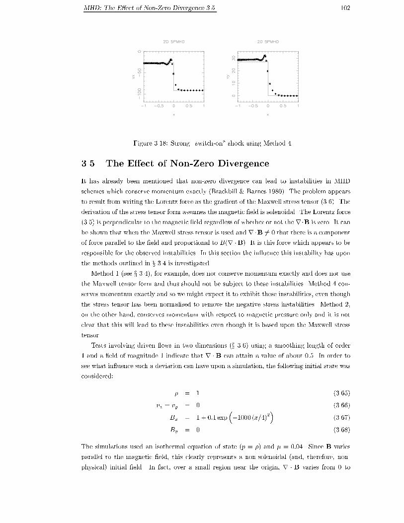
MHD: The E�ect of Non-Zero Divergence 3.5 102
Figure 3.18: Strong \switch-on" shock using Method 4.
3.5 The E�ect of Non-Zero Divergence
It has already been mentioned that non-zero divergence can lead to instabilities in MHD
schemes which conserve momentum exactly (Brackbill & Barnes 1980). The problem appears
to result from writing the Lorentz force as the gradient of the Maxwell stress tensor (3.6). The
derivation of the stress tensor form assumes the magnetic �eld is solenoidal. The Lorentz force
(3.5) is perpendicular to the magnetic �eld regardless of whether or not the r�B is zero. It can
be shown that when the Maxwell stress tensor is used and r�B 6= 0 that there is a component
of force parallel to the �eld and proportional to B(r �B). It is this force which appears to be
responsible for the observed instabilities. In this section the in uence this instability has upon
the methods outlined in x 3.4 is investigated.
Method 1 (see x 3.4), for example, does not conserve momentum exactly and does not use
the Maxwell tensor form and thus should not be subject to these instabilities. Method 4 con-
serves momentum exactly and so we might expect it to exhibit these instabilities, even though
the stress tensor has been normalised to remove the negative stress instabilities. Method 2,
on the other hand, conserves momentum with respect to magnetic pressure only and it is not
clear that this will lead to these instabilities even though it is based upon the Maxwell stress
tensor.
Tests involving driven ows in two dimensions (x 3.6) using a smoothing length of order
1 and a �eld of magnitude 1 indicate that r �B can attain a value of about 0:5. In order to
see what in uence such a deviation can have upon a simulation, the following initial state was
considered:
� = 1 (3.65)
v
x
= v
y
= 0 (3.66)
B
x
= 1 + 0:1 exp
�
�1000 (x=4)
2
�
(3.67)
B
y
= 0 (3.68)
The simulations used an isothermal equation of state (p = �) and � = 0:04. Since B varies
parallel to the magnetic �eld, this clearly represents a non-solenoidal (and, therefore, non-
physical) initial �eld. In fact, over a small region near the origin, r � B varies from 0 to

MHD: The E�ect of Non-Zero Divergence 3.5 103
Figure 3.19: The evolution of the kinetic energy per unit mass using Method 2 (left)
and Method 4 (right) with an initial 10% perturbation to the magnetic �eld. � =
�
B
= � = 0.
Figure 3.20: The evolution of the kinetic energy per unit mass using Method 2 (left)
and Method 4 (right) with an initial 10% perturbation to the magnetic �eld. � = 1,
�
B
= 1 and � = 2.

MHD: Testing the Evolution of the Field in 2D 3.6 104
about �0:4 to about 0:4 and back to zero. The curl of this initial magnetic �eld is zero, so
j is zero. Thus, the Lorentz force is zero. Method 1 evaluates the Lorentz force by taking
the cross-product of j and B and, thus, no uid motion or �eld evolution results. However,
Method 2 and Method 4 use the gradient of the Maxwell tensor to estimate the Lorentz force.
For this non-physical initial �eld, the gradient of the Maxwell tensor results in a force parallel
to the �eld. By modelling the evolution of this system using Method 2 and Method 4 we can
investigate to what extent this force may disrupt the solution.
The results presented in Fig. 3.19 used � = �
B
= � = 0 while those in Fig. 3.20 used
� = 1, �
B
= 1 and � = 2. The quintic spline was used with h = 1:2 particle spacings to
ensure that observed instabilities were the result of non-zero r � B and not two-dimensional
low-order spline instabilities (see x2.6). The particles were placed on a square lattice 0:1 units
apart spanning a region 2 units by 1 unit.
The evolution of the logarithm to base 10 of the kinetic energy per unit mass is plotted.
On these plots, the internal energy per unit mass of the gas corresponds to about 0. Results
are not displayed for Method 1 since there was no evolution of kinetic energy (the Lorentz
force being zero). Methods 2 and 4 both exhibited substantial increases in kinetic energy
(Fig. 3.19). In the case of Method 2 and 4 the initial perturbation in B exerts a force which
leads to an initial increase in kinetic energy. With Method 2, however, the initial disturbance
releases its energy and the kinetic energy of the system remains at about 1% of the internal
energy of the gas. When Method 4 was used the resulting kinetic energy is several orders
of magnitude larger. With the introduction of viscosity (Fig. 3.20) the kinetic energy using
Method 2 undergoes oscillations of diminishing amplitude. Method 4 starts to exhibit this
behaviour before a more serious instability sets in which increases the systems kinetic energy
until it is comparable with the internal energy of the gas.
Although more investigation is required to understand the instability in detail Method 1
should be immune to it. Method 4 is, apparently, most susceptible to the instability resulting
from non-zero divergence of B. The results obtained with Method 2 seem to indicate that,
while there is an initial release of potential energy associated with the non-equilibrium nature
of the initial conditions, the kinetic energy does not grow as much. The tentative conclusion
is that small deviations from a solenoidal �eld will not lead to substantial errors if Method 1
or Method 2 (or 3) are used. What is meant by a \small" deviation, however, depends upon
the various scales involved in the problem and the relative in uence of magnetic forces.
3.6 Testing the Evolution of the Field in 2D
As a test of the method's ability to model the evolution of B we can move the particles
according to a prescribed velocity �eld with some initial magnetic �eld in prescribed two-
dimensional ows. This can be thought of as the limit where � ! 1 and the magnetic �eld
has no feed-back upon the uid motion. In the following sections, results obtained using
SPMHD with two sample ows (shear ow and a single eddy) are compared with exact or
other numerical results.

MHD: Testing the Evolution of the Field in 2D 3.6.2 105
3.6.1 Shear Flow
We consider a simple shear ow
v
x
=
(
V
2(y mod L)
L
if y mod L < L=2
V
2L�2(y mod L)
L
if y mod L � L=2
(3.69)
v
y
= 0 (3.70)
This ow is periodic in y over a distance L. For convenience we will model the ow using
periodic boundary conditions in the x direction also over a distance of L. Taking v = v
x
i and
B = B
x
i+B
y
j in (3.14) we �nd
@B
@t
=
@
@y
(v
x
B
y
)i�
@
@x
(v
x
B
y
)j (3.71)
If the initial �eld is independent of x, this can be further simpli�ed to
@B
x
@t
=
@
@y
(v
x
B
y
); (3.72)
and only the x-component of magnetic �eld changes. We will consider an initial �eld, B = B
0
j,
where B
0
is constant. Then (3.72) reduces to
@B
x
@t
= B
0
dv
x
dy
(3.73)
and has the solution
B
x
=
(
B
0
2V
L
t if (y mod L) < L=2;
�B
0
2V
L
t if (y mod L) � L=2
(3.74)
B
y
= B
0
(3.75)
(3.75) should, for the most part, be a straightforward result to reproduce, since it really
only depends on evaluating the gradient of v and integrating with su�cient accuracy in time.
However, of interest, is how SPMHD simulates the discontinuities in B which develop at y = 0
and y = L=2.
The simulations employed the cubic spline kernel with h = 1:2 particle spacings. The
particles were initially placed on a square lattice one unit apart and L = 40 was used. See
Fig. 3.21 for the case of L = 40, V = 1 and B
0
= 1 at time t = 100. The �eld is correct to
within 3%. The discontinuities at y = 0 and y = L=2 are spread over about three smoothing
lengths.
3.6.2 A Single Eddy
The previous test, although leading to a growing �eld, did not cause the �eld lines to be
wrapped up. We will consider the ow:
v
x
= V
32
�
Y (1� 4Y
2
)
3
cos (�X) (3.76)
v
y
= �V (1� 4Y
2
)
4
sin (�X) (3.77)
� 1=2 � X � 1=2 and � 1=2 � Y � 1=2
where X = x=L�1=2 and Y = y=L�1=2. Outside the region described above, the ow is zero.
A plot of the streamlines appears in Fig. 3.22a. This ow was considered by Weiss (1966) as
part of an investigation of ux expulsion by eddies.

MHD: Testing the Evolution of the Field in 2D 3.6.2.1 106
Figure 3.21: The x component of the magnetic �eld at time t = 100 with L = 40,
V = 1 and B
0
= 1. The solution obtained is correct to within 3%.
3.6.2.1 Reproducing a Steady Result
We will �rst use this ow to test the ability of SPMHD to reproduce steady results where �eld
generation and dissipation are in equilibrium. We will consider the case of R
m
= 40, taking
L = 40, � = 1 and V = 1 and an initial vertical �eld.
Figure 3.22: Solution obtained by Weiss (1966). On the left are the streamlines of
the ow. The �eld lines of the steady state for R
m
= 40 are displayed to the right.
When using an Eulerian technique reproducing such a test case is relatively easy since the
steady-state implies the quantities at the grid points are constant. With Lagrangian techniques,
however, the steady state involves an equilibrium between magnetic �eld generation resulting
from the motion of the grid points and the dissipation. The �eld values at the grid points
are constantly changing as they follow the uid motion. Thus, this problem can be a good

MHD: Testing the Evolution of the Field in 2D 3.6.2.2 107
Figure 3.23: Steady solution obtained using SPMHD after 1600 time units. The
steady state is reached much earlier, however to prove the SPMHD simulation is
stable, it was integrated for much longer. See text for details.
test of the ability of SPMHD to model the simultaneous formation and removal of �eld. It
is, however, somewhat di�cult to generate �eld lines given the SPMHD results. To do this
the particle �eld quantities were interpolated to a regular grid. To generate the �eld lines,
equi-spaced initial points were chosen along y = 0 and y = L and paths tangential to the
magnetic �eld were solved for by using bi-linear interpolation from the regular grid.
The �eld lines obtained by Weiss (1966) appear in Fig. 3.22. The results obtained with
SPMHD (see Fig. 3.23) compare quite well. The lines in Fig. 3.23 appear to be tangential
to those obtained by Weiss (1966). There are some discrepancies, however. The �eld lines in
Fig. 3.22 are not necessarily perpendicular to the upper and lower boundaries. Weiss (1966)
assumed the upper and lower boundaries to be in�nitely conducting. The SPMHD simulation
used �xed boundary particles of constant vertical �eld at the upper and lower boundary,
which forces the �eld to be perpendicular near these boundaries. The �eld lines obtained with
SPMHD do not have matching horizontal intercepts on y = 0 and y = 40. This is possibly a
combined result of interpolation errors and integration errors in producing the �eld lines.
3.6.2.2 Maintenance of a Solenoidal Field
If no dissipation is present, the curling up of the �eld leads to features which cannot be resolved
and the magnetic �eld becomes disordered. This also leads to r � B becoming substantially
non-zero. The following simulations took V = 1 and L = 40 and an initially vertical �eld.
The simulations employed the cubic spline kernel with h = 1:2 particle spacings. The particles
were initially placed on a square lattice one unit apart and L = 40 was used.
The results obtained with � = 0 (Fig. 3.24) show that the initially vertical �eld is curled

MHD: Testing the Evolution of the Field in 2D 3.6.2.2 108
Figure 3.24: In the absence of the any explicit dissipation, the magnetic �eld rapidly
becomes disordered. The arrow heads indicate the direction of the �eld, while their
colour indicates positive (blue) and negative (red) divergence. In black and white,
regions of low divergence appear black and regions of high magnitude divergence (1
in these units) light grey. The �eld was evolved using (3.16).
Figure 3.25: With no arti�cial dissipation, the maximum of the absolute divergence
(dotted line) quite rapidly exceeds 1 as the particle �elds become disordered and
continues to grow. The average magnitude of the divergence steadily increases with
time. The magnetic �eld is evolved using (3.16).

MHD: Testing the Evolution of the Field in 2D 3.6.2.2 109
up and becomes quite disordered. Regions of light colour (or light grey on black and white
reproductions) indicate that the local estimate of divergence is becoming order one. A plot of
the evolution of r � B (see Fig. 3.25) shows that the maximum value of the divergence over
all particles rapidly exceeds 1 and the average over the particles steadily increases with time.
The introduction of some dissipation reduces this problem.
We will investigate the relative merits of the arti�cial dissipation (3.20) and a real, small
dissipation (3.19) in reducing deviations from a solenoidal �eld. To make a reasonable com-
parison, we need to choose � for the real dissipation such that the e�ective magnetic Reynolds
number is the same as that for the arti�cial dissipation (3.23). Thus we solve
R
m
=
8V L
�
B
v
A
h
=
V L
�
(3.78)
and let
� =
�
B
v
A
h
8
: (3.79)
We see this modi�ed real dissipation is reduced as the resolution is increased or the magnetic
�eld is reduced (since v
A
=
p
B
2
=��).
Figure 3.26: The �eld obtained if �
B
= 1 is used. Once again the arrow heads indicate
the direction of the �eld, while their colour indicates positive (blue) and negative (red)
divergence. In black and white, regions of low divergence appear black and regions of
high magnitude divergence (1 in these units) light grey. We see that the orientations
of the arrow heads are less haphazard than those of Fig. 3.24 and that the divergence
remains much smaller.
Using either �
B
= 1 or the modi�ed real dissipation the \complexity" of the magnetic �eld
is kept at the level of resolution of the simulation. Since the arti�cial dissipation preferentially
removes variations of lengthscale h, the resulting �eld is smoother and has much smaller values
for the divergence (see Fig. 3.26 and Fig. 3.28). The maximum magnitude of the divergence

MHD: Testing the Evolution of the Field in 2D 3.6.2.2 110
Figure 3.27: The evolution of r � B with �
B
= 1 and using (3.16). The maximum
of the absolute divergence (dotted line) peaks at approximately 1:7. The average
magnitude of the divergence (the solid line) appears stable at approximately 0:1.
Figure 3.28: The �eld obtained if the modi�ed real dissipation is used (3.79). Once
again the arrow heads indicate the direction of the �eld, while their colour indicates
positive (blue) and negative (red) divergence. In black and white, regions of low
divergence appear black and regions of high magnitude divergence (1 in these units)
light grey. We see that the orientations of the arrow heads are less haphazard than
those of Fig. 3.24 and that the divergence remains much smaller.

MHD: Testing the Evolution of the Field in 2D 3.6.2.2 111
Figure 3.29: The evolution of r�B with the modi�ed real dissipation and using (3.16).
The maximum of the absolute divergence (dotted line) peaks at approximately 1:7.
The average magnitude of the divergence (the solid line) appears stable at about 0:1.
peaks at about 1:7 in both cases and the average value stabilises around 0:1. The peak in
the divergence appears to be the result of the initially regular lattice becoming disordered and
producing substantial voids. In a real simulation the resulting pressure gradients would tend
to close such gaps so we would expect lower values for the divergence.
These results seem to indicate that there is no substantial advantage to using an arti�cial
dissipation of the form (3.20) over a modi�ed form of real dissipation (3.19). Although in the
vicinity of x = 2, y = 5 the results obtained with the arti�cial dissipation (Fig. 3.26) exhibit
slightly less divergence than those using the modi�ed dissipation (Fig. 3.28). Further tests are
required to determine if there are circumstances under which one form provides measurably
better results than the other.
Results were also obtained using (3.18) to evolve the magnetic �eld to see if there was any
advantage in using one or other equation to update the �eld. The results were qualitatively
similar, however, the the divergence was generally 50% larger when (3.18) was employed.

MHD: Conclusion 3.7 112
3.7 Conclusion
We have seen that the results obtained by applying stability analysis to SPH (Chapt. 2) can
be incorporated into a practical approach to modelling MHD with SPH. In particular, the
method whereby the magnetic stress tensor is split to guarantee conservation of momentum
and energy with respect to hydrodynamic and magnetic pressures appears quite robust for
relatively strong magnetic shocks.
The issue of maintaining the solenoidal nature of the magnetic �eld can be dealt with
to some extent by using an arti�cial dissipation (3.20) or a modi�ed form of real dissipation
(3.79) which keeps the �eld smooth over a resolution length. A non-solenoidal �eld will induce
instabilities when a momentum-conserving implementation of SPMHD is used. The tests con-
ducted here suggest that when using the split tensor formulation, for example, small deviations
from a solenoidal �eld will cause relatively small errors. However, further tests are necessary
to con�rm this under more general circumstances and quantify the degree to which the �eld
must be kept solenoidal for SPMHD to be both stable and accurate. Ideally, the arti�cial
dissipation should only be introduced where it is needed, possibly by using a switch similar to
that presented in Chapt. 5.
The issue of modelling con�gurations containing rare�ed regions threaded by strong mag-
netic �elds has not been addressed here. It would seem, however, that SPMHD is most useful
when modelling problems where the important physical processes involving magnetic �elds are
occurring within denser clumps of matter inside a larger computation. SPMHD can readily be
coupled with a tree code (Hernquist & Katz 1989), thus permitting self-gravitating systems
involving MHD to be simulated. Since SPMHD can dynamically increase resolution in regions
of high density, it is not necessary to use complicated grid-re�nement techniques to model
complicated collapse problems. If the problem concerns only a single, relatively stationary,
non-self-gravitating object, then a grid-based code will probably be more accurate.

Chapter 4
Closed Pulsar Magnetosphere
\... what happens at the equator? Maybe the water drains straight down, with no
swirling, or maybe it doesn't drain at all..."
Umberto Eco, Foucault's Pendulum
This chapter introduces a method for simulating the dynamic interaction of a closed magne-
tosphere with an external, �eld-free plasma. The external plasma is modelled using Smoothed
Particle Hydrodynamics (SPH). The method SPH was developed to model astrophysical, com-
pressible hydrodynamics (Gingold & Monaghan 1977, Benz 1989, Monaghan 1992). SPH is
a particle based, fully Lagrangian method which can be readily applied to problems with
complicated geometry. Results obtained using SPH, however, can be less accurate than other
techniques tailored for a speci�c problem. In this application, we are seeking to take advantage
of SPH's ability to model problems involving irregular shaped, dynamic boundaries.
Much work has been done on the modelling of closed magnetospheres. Initially people were
concerned with the Earth's magnetosphere. The earliest work involved �nding the equilibrium
solution for a dipole surrounded by a plasma of constant pressure (Midgley & Davis 1962, Slutz
1962) as a model of the Earth's magnetosphere. The deformation of the Earth's magnetosphere
by the solar wind was �rst looked at by Midgley & Davis (1963), Mead (1964), Mead & Beard
(1964), Mead (1964) and Midgley (1964). In this case people considered the equilibrium
between the magnetic pressure of a dipole and the ram pressure of a cold stream of plasma (an
idealised solar wind). In more recent times people have modelled planetary magnetospheres
(Cheng 1992, Mauk 1994). For an overview of planetary magnetospheres see Lyons & Williams
(1984).
There is a long history of the modelling of pulsar magnetospheres. We are more interested
in problems involving accretion, but �rst we shall give a brief overview of the work done in
solving for the electromagnetic �elds and particle densities in the magnetospheres of pulsars
in general. The �rst work (Goldreich & Julian 1969) looked at the case where the rotation
and dipole axis were aligned. They divided this problem into two regions, one inside and one
outside the light cylinder (R
l
= c=, where c is the speed of light and the angular frequency of
rotation). They assumed that plasma on �eld lines which closed within the light cylinder would
113

MAGNETOSPHERES 4 114
Figure 4.1: The observed pulse period of Vela X-1 (Anzer & Boerner 1994).
corotate with the pulsar, while the plasma on other �eld lines could stream to in�nity. Work
was done for the case of the dipole and rotation axes being perpendicular (Parish 1974). It was
also possible to include inertial e�ects (Scharlemann 1974, Kuo-Petravic, Petravic & Roberts
1975). These models, however, were not entirely self-consistent and, among other things,
had trouble conserving charge (ie- closing the ow of current). Self-consistent electrospheres
of �nite extent were modelled by Krause-Polstor� & Michel (1985a) and Krause-Polstor�
& Michel (1985b). They used an N-body technique to follow the evolution to equilibrium
of a star emitting charge into its electrosphere. Since the problem was axi-symmetric the
particles were actually \rings". A more general approach, employing a boundary element
method to solve for equilibrium con�gurations in three dimensions, was proposed by Shibata
(1989b). The results obtained using this method (Shibata 1989a) agree with those obtained
by Krause-Polstor� & Michel (1985b). More recently, Shibata (1991) modelled the global
structure of such a system using a circuit model. Mestel & Pryce (1992) presented a simple
model pulsar magnetosphere using mathematical techniques which might be of use in more
realistic models. Zachariades (1993) performed a numerical simulation of the aligned rotator
using a two-component plasma model. Mestel & Shibata (1994) presents another model of an
axisymmetric pulsar magnetosphere which includes relativistic e�ects within the light cylinder
and suggests dissipation zones as possible sources of intense X- and gamma-ray emission.
Many authors have studied the accretion properties of pulsar magnetospheres. For an
overview of accretion powered x-ray pulsars, see Nagase (1989). Since the magnetosphere is
so tenuous relative to the external plasma it is potentially unstable to interchange (Rayleigh-
Taylor) instabilities. A rotating magnetosphere may also induce Kelvin-Helmholtz instabilities
at the magnetospheric boundary. In Arons & Lea (1976b), the shape of a non-rotating mag-
netosphere was determined for the case of steady, spherical accretion. This same paper and
Arons & Lea (1976a) investigated the stability properties of the magnetopause with respect
to interchange instabilities and the role this plays in allowing material to be accreted into the
magnetosphere. These processes are also investigated by Elsner & Lamb (1977) and a com-
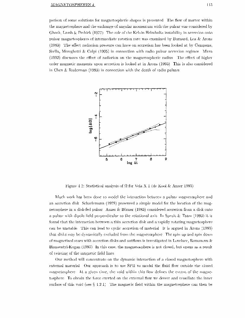
MAGNETOSPHERES 4 115
parison of some solutions for magnetospheric shapes is presented. The ow of matter within
the magnetosphere and the exchange of angular momentum with the pulsar was considered by
Ghosh, Lamb & Pethick (1977). The role of the Kelvin Helmholtz instability in accretion onto
pulsar magnetospheres of intermediate rotation rate was examined by Burnard, Lea & Arons
(1983). The e�ect radiation pressure can have on accretion has been looked at by Campana,
Stella, Mereghetti & Colpi (1995) in connection with radio pulsar accretion regimes. Mitra
(1992) discusses the e�ect of radiation on the magnetospheric radius. The e�ect of higher
order magnetic moments upon accretion is looked at in Arons (1993). This is also considered
in Chen & Ruderman (1993) in connection with the death of radio pulsars.
Figure 4.2: Statistical analysis of for Vela X-1 (de Kool & Anzer 1993).
Much work has been done to model the interaction between a pulsar magnetosphere and
an accretion disk. Scharlemann (1978) presented a simple model for the location of the mag-
netosphere in a disk-fed pulsar. Anzer & B�orner (1983) considered accretion from a disk onto
a pulsar with dipole �eld perpendicular to the rotational axis. In Spruit & Taam (1993) it is
found that the interaction between a thin accretion disk and a rapidly rotating magnetosphere
can be unstable. This can lead to cyclic accretion of material. It is argued in Arons (1993)
that disks may be dynamically excluded from the magnetosphere. The spin up and spin down
of magnetised stars with accretion disks and out ows is investigated in Lovelace, Romanova &
Bisnovatyi-Kogan (1995). In this case, the magnetosphere is not closed, but opens as a result
of twisting of the magnetic �eld lines.
Our method will concentrate on the dynamic interaction of a closed magnetosphere with
external material. Our approach is to use SPH to model the uid ow outside the closed
magnetosphere. At a given time, the void within this ow de�nes the extent of the magne-
tosphere. To obtain the force exerted on the external ow we detect and tessellate the inner
surface of this void (see x 4.2.1). The magnetic �eld within the magnetosphere can then be
MAGNETOSPHERES 4 116
obtained (see x 4.1 and x 4.2.2) and the magnetic pressure exerted on the external plasma
calculated. The model used in this work to obtain the magnetic pressure for a given shape of
magnetosphere is relatively simple and relies on several assumptions (see x 4.1). It is relatively
straightforward, however, to use a more sophisticated technique to solve for the magnetic �eld
in the magnetosphere. We are looking mostly at wind accretion, but it is possible that, in
some circumstances this, or a similar model, could be used to investigate the interaction of a
closed magnetosphere with a disk.
This study was motivated by a desire to model some of the random variations of pulse
period observed in wind fed systems (Harding, Shinbrot & Cordes 1990, Anzer & Boerner
1994). For example, the observed pulse period of the X-ray pulsar Vela X-1 is shown in
Fig. 4.1. The optical component of Vela X-1 is a B 0.5 Ib supergiant. The mass of the
neutron star is about 1:8M
�
, the X-ray luminosity is 3�10
36
erg=s, the orbital period is about
8:96 days, and the orbital separation is 3:7 � 10
12
cm. A statistical analysis of the angular
frequency ((t) = 2�=P (t)) was performed by de Kool & Anzer (1993) and it was found that
the relation j�j = C
p
�tj holds over many decades (see Fig. 4.2). They concluded that the
period variation was a random walk process with amplitude C.
There are many explanations for random variations in pulse period. The study of internal
torques within the super uid interior of neutron stars provides a possible explanation of the
\glitches" observed in period curves (Link & Epstein 1996). Torque variations within the mag-
netosphere, resulting from the motion of plasma towards the poles will also lead to variations
in pulse period. However, these alone will not explain the magnitude of the random walk vari-
ations. External angular momentum variations may provide an explanation for the observed
amplitude of the random walk process. Unstable wind accretion ows can lead to variations in
the angular momentum of the material accreted onto the neutron star. At this time, however,
the size of the variations predicted by numerical simulations is an order of magnitude short of
generating the observed variations in pulse period (Ru�ert & Arnett 1994, Anzer & Boerner
1994). It is possible, however, that a small disk of material could be present in such systems,
and acts as a \reservoir" of angular momentum. Anzer & Boerner (1994) suggested that mass
uctuations within Keplerian disks could explain the observed random walk in pulse period.
The basic idea may be explained as follows. If the material falling towards the magnetosphere
is �eld-free and highly conducting, the magnetosphere may become con�ned to a �nite volume
(see Fig. 4.3). Infalling material will shock and slow as it approaches the magnetopause. This
material may then be spun up by the rotating magnetosphere. Centrifugal forces will cause the
material to ow towards the equator. If the equatorial radius of the magnetosphere extends to
the corotation radius, the material may leave the magnetopause before it is accreted. Thus, a
small disk or torus of material may form in the equatorial plane (see Fig. 4.4). This disk can
now act as a reservoir of angular momentum. As material is fed into the disk, the pulsar spins
down. From the inner edge of the disk the plasma may stream along �eld lines to the magnetic
poles. Depending on the exact nature of this process, the pulsar may be spun up or down.
The important result is that instabilities in such a disk could lead to random variations in the
pulse period. The study of the global interaction of a magnetosphere with external material
is crucial to investigating this model.

MAGNETOSPHERES 4 117
Figure 4.3: Infalling, �eld-free material con�nes the magnetosphere to a �nite volume.
Figure 4.4: Provided the magnetosphere extends to the corotation radius, material
may be spun into orbit before it is accreted. This will lead to the formation of a small
disk or torus of orbiting material.
MAGNETOSPHERES: The Model 4.1 118
4.1 The Model
We will make assumptions similar to those used in Arons & Lea (1976b), however, we will not
assume a steady con�guration. We will assume that the material outside the magnetosphere
is �eld-free and highly conducting. We will assume that the inward ow of this material leads
to a closed magnetosphere about the source. In order to simplify the equations describing the
magnetosphere itself, we will make some further assumptions.
Since the Alfv�en speed (see x 3.2) varies inversely with the square root of the density, v
A
will be very large inside the magnetosphere. If we were to model the magnetosphere with
SPMHD (Chapt. 3) then the CFL condition (x 1.3.2) would require an impractically small
time step. To avoid solving the full MHD problem, we will make some further simplifying
assumptions. We will assume that the magnetosphere is su�ciently tenuous that we need
only consider magnetic �elds due to the currents in the magnetopause and the source itself.
That is, contributions to the magnetic �eld from currents in the interior are negligible. We
also assume that the behaviour of the magnetosphere is quasi-static on the time-scale of the
motion of the external plasma. This means that the magnetosphere responds so rapidly to
the external forces that it is always \steady". External motion will simply cause it to move
into a new, consistent \steady" (quasi-static) state. This requires that the Alfv�en speed is
su�ciently large that
v
A
� L=T and v
A
� R (4.1)
where L is the maximum lengthscale representative of variations in the external ow and T is
the minimum time scale, is the rotation rate of the magnetosphere and R is its radius.
These assumptions reduce the solution of the magnetospheric �elds to a surface integral. It
is possible to make di�erent assumptions (such as those leading to a \force-free" formulation
(Aly 1986)) but these will involve more work in solving for the magnetic �eld. Since we are,
at �rst, concentrating on analysing the dynamic interaction between the external plasma and
the magnetosphere, the simpler approximation for the magnetic �elds is a convenient starting
point.
Consider Maxwell's equations:
r � E =
�
q
�
0
; (4.2)
r �B = 0; (4.3)
r�E+
@B
@t
= 0; (4.4)
r�B� �
0
�
0
@E
@t
= �
0
j (4.5)
where E and B are the electric �eld and magnetic �eld respectively. The charge density and
current density are �
q
and j, and the permittivity and permeability of free-space are �
0
and
�
0
.
Our assumption that the magnetosphere is quasi-static on the time-scales we are con-
sidering allows us to neglect the time-derivatives in these equations. On the interior of the
magnetosphere (except at the source itself), we have j � 0 by assumption, so r�B = 0. This
means that we can write
B = r (4.6)

MAGNETOSPHERES: The Model 4.1 119
(where is a scalar potential) inside the magnetosphere except at the source. Substituting
this into (4.3) we obtain
r
2
= 0 (4.7)
on the interior except at sources. Outside the magnetosphere, there is no magnetic �eld (by
assumption). The currents present in the surface of the magnetosphere act to shield material
outside from the magnetic �eld due to the source. Since B = 0 just outside the magnetosphere,
(4.3) requires that the magnetic �eld at the surface must be parallel to the surface of the
magnetosphere. Thus, we require
@
@n
= 0 at the magnetopause. (4.8)
Here n denotes a co-ordinate in the direction of the outward surface normal. We can now
apply Green's Second Formula
Z
V
fr
2
g � gr
2
fdV =
Z
S
f
@g
@n
� g
@f
@n
dS (4.9)
where V is the volume bounded by the surface S with outward pointing normal n and f and
g are arbitrary functions of appropriate smoothness. We apply this formula to the interior
volume of the magnetosphere with the exception of an arbitrarily small volume about the
source. We take f = 1=(4�r) and g = and obtain (Stratton 1941)
t
=
i
+
1
4�
Z
s
�
1
�r
@
t
@n
�
t
@
@n
�
1
�r
��
dS (4.10)
where
t
is the resulting total potential and
i
is the potential due to internal charges and
currents. This result was obtained using (4.7) and
Z
V
f (r
0
)r
2
�
�1
4��r
�
dV = f (r) : (4.11)
Throughout we are using �r to denote jx
0
�xj where x
0
is the position of the surface element
dS.
If the source is a dipole, for example, we take
i
=
�
0
M cos �
4�r
2
(4.12)
whereM is the dipole moment. From now on we will let denote
t
. We will also assume that
the source is a dipole, but it is trivial to modify the equations for some other given potential.
We can write
@
@n
�
1
�r
�
dS = �d (4.13)
where d is the solid angle subtended at x by the element dS at x
0
. We can now write
=
�
0
M cos �
4�r
2
+
1
4�
Z
S
d (4.14)
where we have applied (4.8). This gives us an expression for the potential at an interior point
in terms of an integral over the surface of the magnetosphere. By considering this equation in
the limit as x approaches the magnetosphere from the inside we see that we have reduced the
solution for the magnetic �eld at the magnetopause to an integral equation.

MAGNETOSPHERES: Numerical Considerations 4.2 120
4.2 Numerical Considerations
4.2.1 Detecting the Magnetosphere
Before we can solve for the force exerted by the magnetosphere at a given time, we must know
its shape. Since we are using a Lagrangian particle method, it is relatively easy to detect the
volume of space the magnetosphere occupies. In our simulations we use particles to describe the
uid. At a given time, there will be a cavity within the uid which de�nes the magnetosphere.
The method used in this work involves dividing the space around the source into sectors. The
br
A
C
B
ra
Figure 4.5: By dividing the space around the source into segments, we can produce a
numerical description of the surface de�ned by the cavity within the particles.
approach is represented in two dimensions in Fig. 4.5. Within each segment we can readily
identify the innermost particle. For segments A and B the radii of the innermost particles are
r
a
and r
b
respectively. The surface of the magnetosphere (a perimeter in two dimensions) is
chosen to pass through the point on the boundary of the two segments which has the average
innermost radius. At the boundary of A and B the point C is on our discrete description of
the magnetosphere with radius (r
a
+ r
b
)=2.
In three dimensions the problem is rather more complicated. Ideally, the solid angle of
each segment would be the same, however, in practice this is relatively hard to achieve. The
problem is basically the same as attempting to tessellate a sphere with equisized polygons to
arbitrary resolution. One of the more convenient tessellations is to simply use points which are
equispaced in spherical coordinates. In this case, however, the segments become very slender
towards the poles. Our method for detecting the magnetospheric surface depends on there
being an adequate number of particles in each segment. Only then can the position of the
boundary be well determined. There are tessellations of the sphere which produce elements
of almost constant size, but the complexity of the algorithm is substantially increased. If the
segments are de�ned in terms of spherical polar coordinates, it is trivial to determine which

MAGNETOSPHERES: Numerical Considerations 4.2.1 121
segment a given particle resides in. This is not the case for more elaborate tessellations. In
this work we have, therefore, used segments de�ned in polar coordinates. As the poles are
approached, the particles in adjacent groups of segments are considered as a whole. This way
the number of particles used to determine the inner radius is kept about constant.
Using spherical polar coordinates:
x = r sin � cos�; (4.15)
y = r sin � sin�; (4.16)
z = r cos �; (4.17)
we de�ne segment ij:
�
i�1
< � < �
i
; (4.18)
�
j�1
< � < �
j
(4.19)
where
�
i
= i��; i = 1; : : : ; N
�
; (4.20)
�
j
= j��; j = 1; : : : ; N
�
: (4.21)
We will let ~r
ij
denote the minimum particle radius within segment ij. It is very straight-
forward to loop over all of the particles, �nd the segment they each reside in, and �nd the
minimum radius for each segment. The solid angle of segment ij is given by
�
ij
= (�
i
� �
i�1
)(cos �
j
� cos �
j�1
); (4.22)
� ���� sin �
j
: (4.23)
So, the solid angle vanishes as we approach � = 0 or � = �. To keep the solid angle over which
the minimum radius is taken about constant, we must take the minimum ~r
ij
of a group of m
adjacent (at the same latitude) segments. We wish the e�ective solid angle to remain about
constant, so
m���� sin �
j
� ����: (4.24)
So we take
m �
1
sin �
j
: (4.25)
However, the groupings of segments must �t evenly around the surface. The easiest way to
ensure this is to choose N
�
to be a power of two, and to consider only groupings of the same
or smaller power of two. Thus, in our method, we take
m = min
�
2
int[� log
2
(min(sin �
j
;sin �
j�1
)+�)]
; N
�
�
: (4.26)
Here � is some quantity small enough to give m = N
�
near the poles, while removing the
singularity in the quotient.
It can also be useful to increase the number of polygons used to describe the magnetosphere
while keeping the e�ective segment sizes the same. In this case, we de�ne groupings in both
the � and � directions
m
�
= min
�
2
int[� log
2
(min(sin �
j
;sin �
j�1
)+�)]
; N
�
�
+ 2
n
tess
;m
�
= 2
n
tess
: (4.27)

MAGNETOSPHERES: Numerical Considerations 4.2.1 122
Generally it was found that taking n
tess
= 0 was adequate for the resolutions used in this
work. So we can now calculate the e�ective minima, m
ij
on each segment:
r
i
0
j
0
; fi
0
= i; : : : ; i+m
�
� 1; j
0
= j; : : : ; j +m
�
� 1g =
min (~r
i
00
j
00
; fi
00
= i; : : : ; i+m
�
� 1; j
00
= j; : : : ; j +m
�
� 1g) : (4.28)
We can now construct a surface based on this information. The vertices at the boundaries of
the collections of segments will have a radius, R
ij
which is the average of the surrounding r
ij
:
R
ij
=
1
4
(r
ij
+ r
i+1j
+ r
ij+1
+ r
i+1j+1
) ; i = 0;m
�
; : : : ; N
�
;
j = 0;m
�
; : : : ; N
�
: (4.29)
In the above expression, the m
ij
must be \wrapped" for i = 0 or i = N
�
. Also, at the poles
(j = 0 or j = N
�
) we simply take the average of all the segments about the pole. The R
ij
interior to the boundary of the segment collections are chosen using bilinear interpolation
R
i
0
j
0
=
�
i
0
� �
i
��
�
R
(i+m
�
�1)j
�R
ij
�
+
�
j
0
� �
j
��
�
R
i(j+m
�
�1)
�R
ij
�
+
�
i
0
� �
i
��
�
j
0
� �
j
��
�
R
(i+m
�
�1)(j+m
�
�1)
+R
ij
�R
i(j+m
�
�1)
�R
(i+m
�
�1)j
�
+R
ij
: (4.30)
It is now a simple matter to give the coordinates of the vertices, V
ij
, which describe the surface:
x
ij
= R
ij
sin �
j
cos�
i
;
y
ij
= R
ij
sin �
j
sin�
i
;
z
ij
= R
ij
cos �
j
: (4.31)
We could describe each segment of the surface using bilinear patches, but it is su�cient to
split them into triangles
S
ij0
= triangle formed by V
ij
; V
ij+1
; V
i+1j
(4.32)
S
ij1
= triangle formed by V
ij+1
; V
i+1j+1
; V
i+1j
: (4.33)
There are some disadvantages to the approach. Near the poles some of the triangles become
degenerate. This was not found to cause problems with the methods introduced in x 4.2.2
which weight elements by area. It is, however, computationally ine�cient, since the tiles
become smaller towards the poles. In the simulations presented here, the axis of the dipole is
always perpendicular to the pole of the coordinate system. Thus the formation of the cusps
at the poles of the dipole is not a�ected by the coordinate pole, but simply smoothed by the
resolution at the equator of the coordinate system.

MAGNETOSPHERES: Numerical Considerations 4.2.2 123
4.2.2 Obtaining the Field Numerically
We have an integral equation which can be solved to give the potential (and therefore the
magnetic �eld) on the surface of the magnetosphere. Using the approach of x 4.2.1 we can
detect and describe this surface numerically. We can solve for the magnetic �eld and evaluate
the force exerted on the uid due to the magnetic pressure:
P
B
=
B
2
2�
0
: (4.34)
The form of (4.14), however, is not suitable for numerical work since it requires us to
integrate through the point we are considering. For example, if we wish to solve for the
potential at x, the integral over all x
0
on the surface S will pass through the point x. The
contribution at this point will involve evaluating the solid angle subtended by the �nite element
of surface at x about the point x. Even if the surface is not discretized, the integral will be
singular at cusps in the magnetosphere. We can avoid this problem by splitting the integral
(Slutz 1962). We consider a small region of the surface, S
00
, which includes the point x, and
the remainder of the surface, S
0
. As we let the region S
00
shrink we can write:
1
4�
Z
S
00
d =
1
4�
Z
S
00
d; (4.35)
=
1
4�
�
4� �
Z
S
0
d
�
; (4.36)
= �
4�
Z
S
0
d (4.37)
and, substituting into (4.14), we obtain
0 =
�
0
M cos �
r
2
+
Z
S
0
d�
Z
S
0
d: (4.38)
Let us now suppose that the shape of the magnetosphere is described by N discrete segments
�S
i
with centroids x
i
. We now wish to solve the set of linear equations given by
0 =
�
�
0
M cos �
r
2
�
+
X
jnfig
j
�
ij
�
i
X
jnfig
�
ij
; i = 1; :::; N (4.39)
for the potential,
i
, on each discrete element. Here jnfig denotes \all j except j = i". The
solid angle is given by
�
ij
=
n
i
�
d
�x
ij
S
i
�r
2
ij
(4.40)
where �x
ij
denotes x
j
� x
i
. So, given the shape of the magnetosphere in terms of small
elements, we can solve for the potential on each element. Solving (4.39) simultaneously can be
fairly expensive. In practice, we will be evolving the magnetosphere and will have the potential
from the previous time-step already. This provides us with a very good initial guess for the
potential of the current magnetosphere. In practice, then, it is enough to iterate using
1
i
=
�
�
0
M cos �
r
2
�
i
+
P
jnfig
0
j
�
ij
P
jnfig
�
ij
(4.41)
where
0
and
1
denote the previous and new approximations.

MAGNETOSPHERES: Numerical Considerations 4.2.2 124
In order to obtain the magnetic �eld (and thence the magnetic pressure) at the surface
of the magnetosphere, we must obtain the gradient of the potential. This could be done
using some sort of �nite di�erences on the discrete surface, but this approach can introduce
substantial errors near cusps in the surface. It is better to take the gradient of
(x) =
�
�
0
M cos �
r
2
�
+
R
S
0
(x
0
)
n�
c
�x
�r
2
dS
R
S
0
n�
c
�x
�r
2
dS
(4.42)
with respect to x. Here \^" is used to denote the unit vector. This expression was obtained
by re-arranging (4.38) and using
d = �
@
@n
�
1
�r
�
dS =
n �
c
�x
�r
2
dS (4.43)
to show the dependence upon x more explicitly. We see that the only x dependence in the
integrals is introduced by �x. It can readily be shown that
r =
(
Z
S
0
d
"
r
�
�
0
M cos �
r
2
�
+
Z
S
0
r
n �
c
�x
�r
2
!
dS
#
�
�
�
0
M cos �
r
2
+
Z
S
0
d
�
Z
S
0
r
n �
c
�x
�r
2
!
dS
)
=
�
Z
S
0
d
�
2
(4.44)
where
r
n �
c
�x
�r
2
=
3(n ��x)�x
�r
5
�
n
�r
3
(4.45)
So, in summary, we can obtain a numerical approximation to the magnetic pressure by iterating
using (4.41) and then calculating
(r )
i
=
8
<
:
X
jnfig
�
ij
2
4
�
r
�
0
M cos �
r
2
�
i
+
X
jnfig
j
r
n �
c
�x
�r
2
!
ij
�S
j
3
5
�
2
4
�
�
0
M cos �
r
2
�
i
+
X
jnfig
j
�
ij
3
5
X
jnfig
r
n �
c
�x
�r
2
!
ij
�S
j
9
=
;
=
2
4
X
jnfig
�
ij
3
5
2
(4.46)
where
ij
is de�ned by (4.40) and
r
n �
c
�x
�r
2
!
ij
=
3(n
j
��x
ij
)�x
ij
�r
5
ij
�
n
j
�r
3
ij
: (4.47)

MAGNETOSPHERES: Numerical Considerations 4.2.3 125
4.2.3 A Particle Representation of the Magnetosphere Boundary
It is possible to derive analytic forms of SPH boundary condition (see x C) to communicate
the magnetic pressure at the magnetopause to the surrounding plasma. With such boundary
conditions as they are presented in x C each particle would observe the magnetosphere to be
locally at. The force due to the magnetosphere could then be determined using the expressions
in x C. This can be done for very smooth magnetospheres but for more realistic shapes, this
approximation does not hold.
C
b
a
B
D
A
Figure 4.6: In the vicinity of a cusp, the magnetosphere certainly cannot be approxi-
mated as locally at.
In Fig. 4.6 we see that, in the vicinity of a cusp, it is certainly not possible to approximate
the magnetospheric surface by a local plane. If a particle simply feels the in uence of the
nearest surface segment, it can be violently thrown from one \slope" of the cusp (AB) to the
other \slope" (BC). Once it crosses the bisector (BD) it will only feel the in uence from the
other side (BC). It might be possible to somehow combine contributions from near segments
using the boundary forces we have derived, but it is not clear that these combinations give a
realistic boundary force.
In our simulations then, the magnetospheric boundary is actually represented by a number
of SPH particles which exert a pressure equal to the magnetic pressure. These particles are
packed relatively close together to give a close approximation to the shape of the magneto-
sphere. The magnetosphere itself will have a very low density. If we were to attempt to model
the gradient in density across the magnetospheric boundary, it would be smoothed over one
or two resolution lengths (h) of the method. This would lead to large non-physical pressure
gradients at the boundary. Instead, we will use the boundary particles to correct the density of
particles near the magnetosphere. The boundary particles will adopt the density of whichever
free SPH particles they interact with. Typically the kernel used in SPH simulations has com-
pact support. Let the distance over which the kernel is non-zero be r
0
. In Fig. 4.7 we see that

MAGNETOSPHERES: Numerical Considerations 4.2.3 126
ar0
Figure 4.7: Near the magnetospheric boundary particle a must have its density esti-
mate corrected for the region within r
0
which the magnetosphere occupies.
a portion of the boundary is within r
0
of particle a. If we were to only include contributions
from the non-boundary particles, the density of particle a would be substantially lower than
its neighbours. If the spacing of particles representing the magnetosphere is �x
m
, then the
boundary particles should each have mass �
a
�x
3
m
. Letting b denote summation over free SPH
particles and b
0
summation over the boundary particles, we can write
�
a
=
X
b
m
b
W
ab
+ �
a
�x
3
m
X
b
0
W
ab
0
: (4.48)
This gives
�
a
=
X
b
m
b
W
ab
=(1� f
m
) (4.49)
where
f
m
= �x
3
m
X
b
0
W
ab
0
: (4.50)
The quantity f
m
can be thought of as the fraction of space around the particle a which is
occupied by particles representing the magnetosphere. This quantity proves most useful in
identifying those particles which are interacting with the magnetosphere (see x 4.2.4). In the
SPH expressions for the pressure gradient, we use
�
b
0
= �
a
; (4.51)
m
b
0
= �x
3
m
�
a
; (4.52)
p
b
0
=
B
2
b
0
2�
0
: (4.53)

MAGNETOSPHERES: Numerical Considerations 4.2.4 127
4.2.4 Modelling Accretion
The parameter f
m
(see (4.50)) is a suitable indicator of a particle's proximity to the mag-
netosphere. Particles should only be accreted within one or two smoothing lengths of the
magnetospheric boundary. This is consistent with the idea that the position of the boundary
is uncertain to within the resolution length. So we can accrete (ie- remove) a particle with a
probability, P
i
, which is, for simplicity, proportional to f
m
. We will denote f
m
for particle i
by f
i
. Let us suppose that P
i
= kf
i
where k is a constant. The work of Arons & Lea (1976b)
assumed that the magnetosphere was steadily accreting material. Thus, in order to reproduce
their results, it makes sense to derive an accretion probability that can lead to a steady state.
To estimate the appropriate dependence of P
i
upon density and smoothing length, we
consider steady accretion onto a sphere of radius R
�
with plasma density �
�
. If we accrete
particles with the probability P
i
at each time step we expect N
acc
particles to be accreted
where
N
acc
=
X
i
P
i
; (4.54)
=
X
i
�
i
m
i
P
i
�V
i
; (4.55)
�
Z
�
i
m
i
P
i
dV; (4.56)
�
k�
�
m
Z
fdV; (4.57)
�
k�
�
m
4�R
2
�
Z
R
�
+r
0
R
�
f(r)dr; (4.58)
where r
0
is the radial extent of the kernel. Typically, the integral evaluates to h=4A where A
is an order one constant. We wish the accretion rate at the magnetopause to be in equilibrium
with the prescribed accretion rate at the outer boundary:
�t
_
M = mN
acc
(4.59)
so
k =
�t
_
MA
�R
2
�
�
�
h
(4.60)
Thus, we could use
P
i
=
A�t
_
M
�R
2
�
�h
i
f
i
; (4.61)
however, it was found that it was better to let the accretion probability depend more strongly
upon the local density, so
P
i
=
A
_
M
�R
2
�
�
2
�
�t�
i
f
i
h
i
(4.62)
where
_
M is the mass ow into the system. This is not consistent with k being constant,
however, the argument serves to give estimate of the appropriate dependence of the accretion
probability on �eld quantities. In practice
A = 2 (4.63)

MAGNETOSPHERES: Numerical Considerations 4.2.4 128
was found to be a good choice, but the exact choice was not crucial. For the case of supersonic
accretion we took the initial radius of the non-equilibrium magnetosphere as R
�
and
�
�
= v
2
�
=c
2
0
�
0
(4.64)
as an estimate of the density at the magnetopause where v
�
and �
0
are the free-fall velocity
and density at the outer boundary condition.
Since the position of the magnetopause depends directly upon the particle positions (x 4.2.1),
removing a particle instantaneously can introduce substantial noise at the accreting boundary.
It is possible to transfer a fraction of a particle's mass according the the accretion probability.
However, this can lead to a large number of small-mass particles being present in the simula-
tion. This is not only computationally expensive but may lead to inaccuracies in interpolation
(see x D). An alternative approach is to mark particles as \accreted" and reduce their mass
by constant decrements until the particle mass is zero. Thus, the deletion of the particle is
\smoothed" over several time steps. In the simulations presented here, N
d
denotes the number
of time-steps over which a particle is deleted.
In more realistic simulations where the accretion process is not assumed to be steady, f
i
should be chosen according to analysis of Rayleigh-Taylor and Kelvin-Helmholtz instabilities.
There was not time for this approach to be explored as part of this study.
MAGNETOSPHERES: Numerical Considerations 4.2.5 129
4.2.5 Modelling the Infalling Material
In problems where we are studying accretion, we need to represent a prescribed ux of matter
across some outer boundary of the numerical model. With SPH this involves introducing a
number of particles at the outer boundary at each time step. Let us �rst consider purely
spherical accretion. The outer boundary of the computational domain will be a sphere of
radius r
out
. The velocity at the outer boundary is assumed to be the free-fall velocity, given
by
v
�
=
r
2GM
r
out
: (4.65)
If the mass- ow rate into the system is
_
M , and the particles are of mass m, then in a given
time step, �t we must introduce
N
in
=
_
M�t
m
(4.66)
new particles. These particles should be evenly spread over a shell of thickness v
�
�t at radius
r
out
. One way to achieve this is to use a volume preserving mapping from a unit cube onto
this shell
� = 2�X;
w = 2
�
Y �
1
2
�
;
r = r
out
� v
�
�tZ;
x = r
p
1� w
2
cos�;
y = r
p
1� w
2
sin�;
z = rw: (4.67)
Here, X , Y and Z are all de�ned on the interval [0; 1]. We could use random numbers for
these variables but this can lead to quite strong uctuations in density at the outer boundary.
It is better to use in�nite sequences which have constant density on the unit interval. In our
work, Halton sequences (see x B) are employed to provide positions for particles in the outer
shell. Sequences of X
j
, Y
j
and Z
j
were obtained by using Halton sequences of base 2, 3 and
5. The material external to r
out
was modelled using the SPH boundary conditions described
in x C.
MAGNETOSPHERES: Test Cases 4.3 130
4.3 Test Cases
4.3.1 Constant External Pressure
As a test case for the method, we now consider the equilibrium shape of the magnetosphere of a
dipole surrounded by a plasma of constant pressure. This problem was considered by Midgley
& Davis (1962) and Slutz (1962) as a simple model of the earth's magnetosphere. This problem,
of course, is axisymmetric and is quite easily solved without resorting to fully three-dimensional
numerical analysis. In Midgley & Davis (1962) the shape of the magnetosphere (see Fig. 4.8)
is found using a moment technique (similar to that used later by Arons & Lea (1976b) with
pulsar magnetospheres). In Slutz (1962) a somewhat similar approach to that of x 4.1 is used.
In Slutz (1962), the discretization is in latitude only and there is a straightforward relationship
between the potential and distances measured on the magnetospheric surface.
A natural lengthscale of the problem can be de�ned in terms of the magnetospheric radius
R
P
m
corresponding to the equatorial radius where the magnetic pressure of the isolated dipole
�eld equals the prescribed, external plasma pressure:
B
2
2�
0
= P
0
: (4.68)
Here
B =
M�
0
4�R
3
(4.69)
and P
0
is the given external pressure. Solving (4.68) for R using (4.69) gives:
R
P
0
=
�
M
2
�
0
32�
2
P
0
�
1=6
: (4.70)
The simulation performed here uses �
0
= 1 and M =
p
32�.
R
e
=R
P
m
R
p
=R
P
m
(Midgley & Davis 1962) 1.41 0.90
This work 1.40 0.98
Table 4.1: Polar (R
p
) and equatorial (R
e
) radii for magnetosphere under constant
external pressure.
To model this problem with our method, we consider a dipole surrounded by plasma con-
tained within a solid sphere. We choose some initial shape for the magnetosphere, a perfect
sphere say, and evolve the system to a steady state. For the results presented here, once the
steady state was reached, P
0
was found to be approximately 0:9 giving:
R
P
0
� 1:02: (4.71)
The equatorial radius of the magnetosphere obtained (see Fig. 4.9) agrees with very well with
Midgley & Davis (1962) (see Table 4.1). The radius at the cusp, however, is almost 9% too
large. This is, primarily, the result of low resolution smearing the cusp region out. A three-
dimensional rendering of the magnetosphere obtained is shown in Fig. 4.10.

MAGNETOSPHERES: Test Cases 4.3.1 131
Figure 4.8: The solid line solution is that obtained by Midgley & Davis (1962) for the
shape of magnetosphere surrounded by plasma of constant pressure. The dashed line
is that obtained by Beard (1960) using a simpler, less accurate boundary condition.
Figure 4.9: The SPH particle positions for constant external pressure for the steady
state. The results are fully three-dimensional, but here the vertical axis is parallel
to the dipole while the horizontal axis is the perpendicular distance from the dipole
axis.

MAGNETOSPHERES: Test Cases 4.3.1 132
Figure 4.10: A three-dimensional rendering of the steady magnetosphere, obtained
with SPH, for constant external pressure. The dipole axis has been tilted towards the
observer to show the cusp at the \north" pole.

MAGNETOSPHERES: Test Cases 4.3.2 133
4.3.2 Steady, Supersonic Accretion
Another test for the method is that of steady accretion. In this problem, a spherically symmet-
ric stream of plasma converges on the magnetosphere. Once again, the problem is axisymmet-
ric and time independent, but provides another test of the method against established results.
The magnetosphere \absorbs" material at some rate which, in the case of steady accretion,
leads to equilibrium between rate of accretion and rate of in ux of material. This particular
problem was considered by Arons & Lea (1976b) in connection with accretion onto a pulsar
magnetosphere.
A natural lengthscale for the problem can be de�ned in terms of the accretion magneto-
spheric radius R
a
m
corresponding to the equatorial radius where the magnetic pressure of the
isolated dipole �eld equals the ram pressure of the free-falling plasma:
B
2
2�
0
= �v
2
�
: (4.72)
Here B is given by (4.69) and
v
�
=
r
2GM
R
: (4.73)
If
_
M is the rate at which material is being fed into the system, then
_
M = 4�R
2
�v
�
: (4.74)
Eliminating � and v
�
using (4.73) and (4.74) we obtain:
�v
2
�
=
_
M
p
2GM
4�
R
�5=2
: (4.75)
Substituting (4.69) and (4.75) into (4.72) and solving for R we obtain:
R
a
m
=
�
M
2
�
0
8�
_
M
p
2GM
�
2=7
(4.76)
(c.f. Eq. 22 in Arons & Lea (1976b) using di�erent units). The simulations presented here
take GM = 1, M = 1, �
0
= 1 and
_
M = 1=4 giving:
R
a
m
=
�
8�
2
�
�1=7
� 0:5357280 (4.77)
R
e
=R
0
m
R
p
=R
0
m
(Arons & Lea 1976b) 1.78 0.91
This work: N
d
= 1 1.77 1.29
N
d
= 5 1.76 1.19
N
d
= 10 1.76 1.12
Table 4.2: Polar (R
p
) and equatorial (R
e
) radii for the accreting magnetosphere.
Let us consider some results obtained using our SPH code with initially 30; 000 particles
using N
d
= 1 (Fig. 4.12 and Fig. 4.13). The Mach number of the ow at the outer boundary

MAGNETOSPHERES: Test Cases 4.3.2 134
Figure 4.11: The solution obtained by Arons & Lea (1976b) for the shape of an
accreting, non-rotating pulsar magnetosphere. Note that the thickness of the shocked
layer is exaggerated by a factor of seven.
is about 2 and the initial state was spherically symmetric free-falling plasma onto a purely
spherical magnetosphere of radius 0:8. Initially the density at the magnetosphere is very low
and so the accretion rate is very small (see Fig 4.12). Material rapidly \piles up" at the magne-
tospheric boundary, producing a post-shock layer. The accretion rate then increases until the
system reaches equilibrium. At this point there are about 54; 000 particles in the simulation.
We see that the accretion rate is somewhat noisy. The magnitude of the uctuations is reduced
with higher resolution. Improved boundary conditions should also reduce this noise.
The solution in Arons & Lea (1976b) (see Fig. 4.11) is scaled such that the equatorial radius
is 1. Our results use a di�erent scaling, but once rescaled we see (Table 4.2) that the equatorial
radii agree to within 1%. The cusp is smeared out and not resolved, so the polar radius of the
magnetosphere in this simulation is larger by about 40% than that obtained by Arons & Lea
(1976b).
Since particles are individually removed over a single time-step the plasma has less chance to
form a steady post-shock layer. This is especially true near the cusps where infalling particles
have a larger region of space around them occupied by the magnetosphere. Fig. 4.14 and
Fig. 4.15 show the density obtained using N
d
= 5 and N
d
= 10 respectively. We see that as
particles are removed over more time steps, the cusp becomes better resolved. The polar radii
(Table 4.2) are still in error by 31% and 23% for the cases of N
d
= 5 and N
d
= 10 respectively.
In Fig. 4.16 the magnitude of the velocity of the particles is displayed as a density plot. The
post-shock layer can be seen as a dark \halo" about the magnetosphere. A three-dimensional
rendering of the magnetosphere appears in Fig. 4.17.

MAGNETOSPHERES: Test Cases 4.3.2 135
Figure 4.12: The accretion rate as a function of time (N
d
= 1). Initially the accretion
rate is zero, but it rapidly increased to become steady as the post-shock layer of
material builds up.
Figure 4.13: The density of material (magnitude of velocity) using N
d
= 1. The hor-
izontal axis is parallel to the axis of the dipole. The vertical axis is the perpendicular
distance from the dipole axis. The image is scaled from white (density of 0) to black
(density of 0:05). We see that a thin layer of post-shock material extends around the
magnetosphere.

MAGNETOSPHERES: Test Cases 4.3.2 136
Figure 4.14: The density of the plasma using N
d
= 5. The same axes are used as in
Fig. 4.13. The image is scaled from white (density of 0) to black (density of 0:05).
The cusp is slightly better de�ned than in Fig. 4.13.
Figure 4.15: The density of the plasma using N
d
= 10. The same axes are used as
in Fig. 4.13. The image is scaled from white (density of 0) to black (density of 0:05).
The cusp is substantially better de�ned than in either Fig. 4.13 or Fig. 4.14.

MAGNETOSPHERES: Test Cases 4.3.2 137
Figure 4.16: The speed of material. The horizontal axis is axis of the dipole. The
vertical axis is the perpendicular distance from the dipole axis. The image is scaled
from white (speed of 1) to black (speed of 0). We see that a thin layer of relatively
slow moving, post-shock material extends around the magnetosphere.
Figure 4.17: The shape of the magnetosphere using N
d
= 10. The dipole axis has
been tilted towards the observer to show the cusp at the \north" pole.

MAGNETOSPHERES: Discussion and Conclusion 4.4 138
4.4 Discussion and Conclusion
We have seen that a method can be developed which extends SPH to model the interaction of
an external �eld-free plasma with a closed pulsar magnetosphere. The method has reproduced
results obtained for some steady con�gurations but exhibits quite large errors near cusps in the
magnetosphere. These errors should be reduced by using higher resolution, however, improved
accretion boundary conditions might also help. The method for tesselating the magnetosphere
(x 4.2.1) leads to uneven resolution over the surface. More elaborate tessellations might permit
the cusps to be better resolved.
There are several immediate extensions which are of interest. We can readily break the
symmetry of the test problems by rotating the dipole slowly (so as to respect (4.1)). It is also
quite simple to model the accretion of material with some given angular momentum.
It is also possible to consider, with our method, the consequences of reducing the accretion
rate or the ux of mass into the system. It may also be possible to consider burst-like ows of
the type presented in Lamb, Fabian, Pringle & Lamb (1977) where the accretion rate is highly
non-steady.
We are also interested in modelling the evolution of an accreting system with a rapidly
rotating magnetosphere. Unfortunately, the model for the magnetosphere itself will break down
under such circumstances (4.1). One could implement a \force-free" model (Aly 1986) of the
magnetosphere to extend the method to handle this case. However, it may be possible to obtain
some basic insight into the behaviour of such a system by assuming that the magnetosphere is
spherical and rigid. In this case, we can prescribe boundary conditions at the magnetopause
using the SPH boundary conditions developed in x C.
It should be possible to implement a more realistic accretion boundary condition based upon
analysis of Rayleigh-Taylor and Kelvin-Helmholtz instabilities. This could involve developing
a viscosity which varies with latitude and relative velocity between the external uid and the
rotating magnetosphere and seeks to mimic the ux of momentum due to instabilities at the
magnetospheric surface. Such improvements might also lead to the cusp of the magnetopause
being better resolved for the steady test cases.

Chapter 5
Shock Detection with SPH
\Like bubbles in a late-disturbed stream..."
William Shakespeare, King Henry IV
SPH simulates shocks by using an arti�cial viscosity. Unlike Eulerian methods it is not
convenient to reduce the e�ects of viscosity by means of switches based on spatial gradients.
In this chapter, a new form of switch for the SPH viscosity is proposed. Each SPH particle has
a viscosity coe�cient which satis�es a di�erential equation designed to increase the coe�cient
near a shock and cause it to decay to a small value elsewhere. Examples applying the switch
to one-dimensional shock problems and to the case of a weak shock striking a bubble con�rm
that the switch is e�ective.
In the numerical solution of compressible gas problems using the Eulerian formulation
shocks were originally simulated by using an explicit arti�cial viscosity or by an implicit vis-
cosity resulting from averaging (Richtmyer & Morton 1967). All these schemes resulted in
substantial smearing of shocks and contact discontinuities together with excessive vorticity
decay. The introduction of switches based on spatial derivatives of suitable variables (van Leer
(1979), Roe (1981), Harten, Lax & van Leer (1983)) gave much sharper shocks. Combined
with Riemann methods with Total Variation Diminishing (TVD) properties (see Toro (1992)
for examples) these methods give outstanding results for the dynamics of ideal gases. Their
only disadvantage is that the methods can be troublesome to implement when the physics is
very complicated, and they can lead to subtle errors (Quirk 1994).
Particle methods such as PIC and SPH are always easy to implement even when the physics
is complicated however, at present, they treat shocks by the use of an arti�cial viscosity which
results in much greater smearing of shocks and vorticity decay than current Eulerian methods.
Some work, however, has been done to incorporate Riemann solvers (Inutsuka 1994, Monaghan
1996) into the SPH formalism. The switches used for Eulerian schemes do not seem to have
any obvious counterpart in Lagrangian particle methods and considerable e�ort has therefore
gone into devising alternative viscosity limiters. The �rst of these is to only turn the viscosity
on when particles are approaching- removing the viscosity for rarefactions. This simple limiter,
unfortunately, does little to reduce viscosity in regions of high vorticity. Other limiters include
139

SHOCK DETECTION: The new switch 5.1 140
using the ratio of the divergence and the curl of the velocity �eld (see Balsara (1995) and (5.1))
to reduce the viscosity when the magnitude of the vorticity is much greater than that of the
divergence.
In this chapter we consider an entirely di�erent viscosity limiter. We give each particle a
viscosity parameter which evolves according to a simple source and decay equation. The source
causes the parameter to grow when the particle enters a shock and the decay term causes it
to decay to a small value beyond the shock.
The standard SPH arti�cial viscosity is presented in x 1.1.5. If the continuum limit of the
equations is taken (by taking the limit as the number of particles goes to in�nity) the arti�cial
viscosity is found to give a shear and bulk viscosity (Pongracic (1988), Meglicki et al. (1993)).
For example, the term with the speed of sound produces a shear viscosity coe�cient of �hc=8
for two-dimensional motion and this is con�rmed by numerical experiments (Maddison et al.
1996, Murray 1996). The typical Reynolds number is therefore 8V L=(�ch) where V is a typical
velocity varying on a length scale L. Since medium to strong shocks require � = 1, and typical
resolutions result in L � 25h the Reynolds number is � 200 for Mach numbers � 1. This
value is acceptable for many simulations but for low Mach number ow, the uid becomes too
viscous and angular momentum and vorticity are transferred unphysically. The limiter due to
Balsara (1995) combats this by multiplying �
ab
by f
ab
where
f
a
=
jr � vj
a
jr � vj
a
+ jr � vj
a
+ �
(5.1)
In cosmological simulations this viscosity limiter reduces the unphysical spread of angular
momentum in galactic disks by a factor 20 (Steinmetz 1996). It has no e�ect on one-dimensional
or planar shocks though it improves results for shocks hitting density discontinuities obliquely.
5.1 The new switch
We give each particle its own viscosity parameter �. This parameter is then assumed to evolve
according to the equation
d�
dt
= �
�� �
?
�
+ S (5.2)
The �rst term on the right hand side of (5.2) causes � to decay to �
?
with e-folding time � .
We assume here that �
?
= 0:1 since this gives an order of magnitude reduction in viscous
e�ects while maintaining order amongst the particles away from shocks. The second term S
is a source which causes � to grow as the particle approaches a shock.
There are many possibilities for the choice of � and S. The time scale really should be
chosen according to the post shock states including the post shock velocity relative to the
shock front. Without knowing the structure of the shock we cannot estimate this accurately.
As a compromise we use
� =
h
C
1
c
; (5.3)
where C
1
is a non-dimensional parameter. This time scale is related to that used by many SPH
codes to chose a suitable time step according to the CFL condition (x 1.3.2). This choice of �
is approximately the time information takes to propagate through a resolution length(h).

SHOCK DETECTION: The new switch 5.1 141
A suitable value for C
1
can be determined by the following argument. Consider (5.2) just
behind a shock, where S � 0 and � is a maximum:
d�
dt
= � (�� �
?
) C
1
c
h
: (5.4)
This has the solution
� = �
?
+A exp
�
�
t
�
�
(5.5)
which describes the exponential decay of viscosity behind the shock. Typically, we want the
viscosity to persist for several smoothing lengths behind the shock. The post-shock velocity
(relative to the shock front) is M
2
c, where M
2
is the post-shock Mach number. If we equate
the time taken to travel h� (relative to the shock front) downstream to the e-fold time, we
obtain
C
1
=
M
2
�
: (5.6)
If we take the limit of in�niteM
1
in the one-dimensional shock jump conditions ((5.23) through
(5.25)) we obtain (5.27) through (5.31). Taking M
2
= jv
2
j=
p
P
2
=�
2
and substituting for P
2
and �
2
using (5.27) and (5.28) we obtain:
M
2
=
r
� 1
2
(5.7)
for in�nite strength shocks. Thus, we choose:
C
1
=
1
�
r
� 1
2
: (5.8)
For = 5=3 we �nd C
1
� 0:447=�. Thus, if we wish the viscosity to decay over 2 to 5 smoothing
lengths, we have
C
1
� 0:1� 0:2 (5.9)
In the calculations described later we choose C
1
= 0:2.
We choose S to be
S = C
2
max(�r � v; 0) (5.10)
since this becomes large near shocks and is Galilean invariant. Other forms of S are discussed
in x 5.3.
We can determine the typical peak values of � by considering a particle approaching a
shock in one dimension. If we assume that the time taken passing through the shock front
(where the source term is largest) is short compared to � , the decay term can be neglected. We
assume that the shock pro�le is steady at x = 0, the uid velocity is in the negative direction
and decreases in magnitude monotonically as uid passes through the shock front (@v=@x < 0).
A frame where the shock front is stationary is chosen to simplify the analysis, but the result
remains Galilean invariant. In this case, the comoving derivative is
d
dt
= v(x)
@
@x
(5.11)
Neglecting the decay term, the equation for �(x) becomes
v
@�
@x
= �C
2
@v
@x
(5.12)

SHOCK DETECTION: Test cases 5.2 142
for our choice of source term. Thus,
�(x) � �
?
= C
2
Z
x
x
0
=+1
�
1
v
@v
@x
0
dx
0
(5.13)
= �C
2
ln
v
v
1
(5.14)
where
lim
x!+1
v(x) = v
1
: (5.15)
Downstream of the shock front
� = �
?
+ C
2
ln
v
1
v
2
(5.16)
where v
2
is the post-shock velocity relative to the shock front. For a shock of in�nite Mach
number in an ideal gas, we have
v
2
= C
2
� 1
+ 1
v
1
(5.17)
and
� = �
?
+ C
2
ln
+ 1
� 1
(5.18)
Our one-dimensional tests used C
2
= 1 and an ideal, monatomic equation of state, leading to
�� �
?
having a theoretical peak of � 1:39 in the absence of the decay term. The presence of
the decay term leads to this peak not being realised. In practice, � was observed to peak at
� 1, which is known from many experiments to be a good choice for shocks. Since the peak
value of � depends upon the equation of state ( in (5.18)), in general, C
2
should be varied for
di�erent choices of . For example, our calculations simulating a shock striking a bubble of
gas used = 1:4, giving a theoretical peak of � 1:79 if C
2
= 1 were used. On the basis of the
one-dimensional results, we took C
2
= 1:39=1:79 � 0:77 to reduce the peak to approximately
1 for strong shocks.
It is also informative to consider the case of a homologous ow
v = �Ar: (5.19)
In astrophysical problems involving gravitational collapse, the ow may approximate this ideal
in some regions and it is important that � remain suitably small in the absence of shocks. This
ow gives a constant source term
�r � v = 3A: (5.20)
Substituting this into (5.2) and considering the steady state, we �nd
� = �
?
+ 3A� (5.21)
= �
?
+
3Ah
C
1
c
(5.22)
We see that for rapidly contracting (large A) systems, � could become quite large. As the
system contracts, however, h should decrease and c increase, leading to a decrease in �. In
practice, an acceptable maximum � for the unshocked uid should be chosen and (5.22) solved
to determine an appropriate resolution (h). For some collapse problems, this resolution may
be too computationally expensive. Similar analysis could be carried out for alternate source
terms which may perform better in such circumstances.

SHOCK DETECTION: Test cases 5.2.1 143
5.2 Test cases
The simulations presented in the following sections use C
1
= 0:2. The exact choice is not
critical, but this value provides good results for a wide range of problems.
5.2.1 Stationary shock front
The simplest test case to consider is that of a one-dimensional shock. We will consider the
problem in the frame of reference of the shock front. The jump conditions can be written
�
2
=
( + 1)M
2
1
2 + ( � 1)M
2
1
�
1
; (5.23)
v
2
=
2 + ( � 1)M
2
1
( + 1)M
2
1
v
1
; (5.24)
P
2
=
2 M
2
1
� ( � 1)
+ 1
P
1
; (5.25)
The subscripts 1 and 2 denote pre- and post-shock conditions respectively. (see Fig. 5.2.1).
The Mach number is de�ned by
M
1
= �v
1
r
�
1
P
1
(5.26)
The upstream particle spacing is 1 unit and the smoothing length is 1:2 units. Constant
PP
v v2
2
1
1
2 1ρ ρ
Figure 5.1: The states for a stationary shock.
smoothing length was used. The gas was taken to be ideal with = 5=3. For strong shocks,
therefore, the particle spacing downstream of the shock is about 0:25 units. Fig. 5.2 shows the
results of one-dimensional SPH simulations of shocks with Mach number 10 on the left and
Mach number 100 on the right. These plots show a close-up view of the particle quantities
about the shock front which is spread over about 3 smoothing lengths. Each column of frames
displays the velocity, source term and �. We see that the source term peaks mid-way in
the slope of the shock front, as expected. The � viscosity peaks as the particles reach their
maximum (least negative) velocity, and decays over several smoothing lengths. When the
Mach number is increased by a factor of 10 the peak in the source term increases by a factor
of 10 also. However, particles are travelling at 10 times the speed they were in the weaker
shock simulation and, thus, spend a tenth of the time passing through the shock front. This

SHOCK DETECTION: Test cases 5.2.1 144
leads to � having practically the same maximum value in both simulations. Furthermore,
since the e-folding time is similar to a time-step condition, it scales appropriately with the
Mach number. There are some small oscillations downstream of the shock which are typical
of standard SPH simulations of this kind and are consistent with the accuracy of the method.
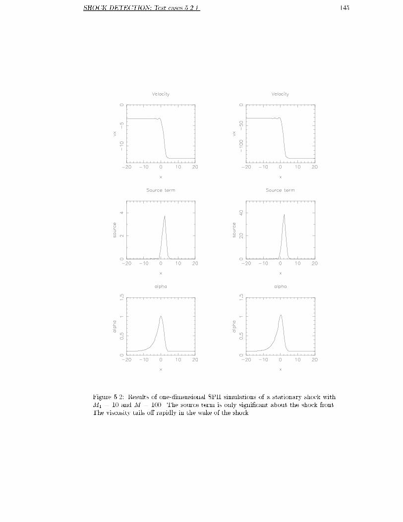
SHOCK DETECTION: Test cases 5.2.1 145
Figure 5.2: Results of one-dimensional SPH simulations of a stationary shock with
M
1
= 10 and M = 100. The source term is only signi�cant about the shock front.
The viscosity tails o� rapidly in the wake of the shock.

SHOCK DETECTION: Test cases 5.2.2 146
5.2.2 Cold streams colliding
An extreme test case, involving shocks, is that of two cool streams of gas colliding head-on
(see Fig. 5.3). Since the streams are initially cold, the speed of sound is very low (0:01 in
P2
2
2
P = 01P = 01
u=v+Vρ
1ρ
VV
u
u = 0
1 1 1
1ρ
Figure 5.3: The states involved in the collision of two cold streams of gas. Here
u = v+V where V is the shock velocity in the frame of reference where u
2
= 0. Thus
V = �v
2
and u
1
= v
1
� v
2
.
the co-ordinates used in this simulation) and the Mach number, very high. Considering the
jump conditions for a one-dimensional shock ((5.23) through (5.25)) in the limit of large Mach
number gives
�
2
=
+ 1
� 1
�
1
(5.27)
P
2
=
2 M
2
1
+ 1
P
1
(5.28)
v
2
=
� 1
+ 1
v
1
(5.29)
u
1
= v
1
� v
2
=
2
+ 1
v
1
(5.30)
V = �v
2
= �
� 1
2
u
1
(5.31)
Again we used an ideal gas with = 5=3. The particle spacing in the cold gas is 1 unit
with a smoothing length of 1:2 units. Results obtained using SPH with the new viscosity are
displayed in Fig. 5.4. The case on the left involves M
1
= 10
3
shock, while that on the right is
M
1
= 10
5
. We see, as before, that the source term peaks strongly at the shock fronts, feeding
the viscosity, which then decays rapidly in the wake of the shocks. Although the source term
has a much higher peak for theM
1
= 10
5
case, the maximum value of � is practically the same.
Again, there are slight oscillations behind the shock, which are consistent with the accuracy
of the method. We see that the same choice of parameters used for the previous test has lead
to appropriate behaviour in � for a wide range of Mach numbers.

SHOCK DETECTION: Test cases 5.2.2 147
Figure 5.4: One-dimensional SPH simulations of cold streams colliding withM
1
= 10
3
.
SPH simulations of cold streams colliding with M
1
= 10
5
. The source term is only
signi�cant about the shock fronts. The viscosity tails o� rapidly in the wake of the
shocks.

SHOCK DETECTION: Test cases 5.2.3 148
5.2.3 A Shock Striking a Bubble
The tests presented so far are one-dimensional and do not test the method's ability to model
ows involving vorticity. In this section we present simulations attempting to reproduce exper-
imental results for a shock striking a bubble of gas (Haas & Sturtevant 1987). This problem
has been solved numerically by many authors including Picone & Boris (1988) and Don &
Quillen (1995). It is an interesting test of a numerical method's ability to model shocks,
contact discontinuities and vorticity generation. The con�guration of the shock tube appears
in Fig. 5.5. Here we will only consider results obtained for the case of a weak shock (Mach
Bubble
ShockP = 1.01 x 10
3
5
v = v = 0x y
y
x
v = V
v = 0
P = P
x 2
y
2
2
Inflow
v = V
v = 0
P = P
x 2
y
2
2
shock tube
Axis of
(perfect reflection)
ρ = ρ
= 1.29 kg/mρ
ρ = ρ
Figure 5.5: The shock tube con�guration used by Haas & Sturtevant (1987) in their
experiments.
number 1:23) striking a dense bubble of gas. The shock tube has a diameter of 8:9 cm and
the cylinder of gas has a density of 4:64 kg=m
3
and radius 2:5cm. The surrounding gas has a
density of 1:29 kg=m
3
.
Typically in standard SPH simulations � is taken to be quite large (often 1) globally. This
is necessary, since the viscosity must be present where there are strong shocks. This simulation
does not involve particularly strong shocks and quite reasonable results may be obtained by
taking � = 0:1. This, however, presumes prior knowledge of the details of the calculation,
and in general applications involve both strong and weak shocks, thus forcing large amounts
of viscosity to be used everywhere. We shall, then, compare results obtained using the new
viscous switch (for the same parameters used in the previous tests) with those obtained using
� = 1.
The simulations presented here used an ideal gas with = 1:4 (as did Picone & Boris
(1988)). Since the peak value of � is expected to be higher for this (5.18), we took C
2
= 0:77.
(5.8) suggests that C
1
should be changed also. However, the correction is so small that C
1
= 0:2
was used as before. Re ecting boundary conditions are used to model the top half of the tube.
The computational domain is spanned by 100 particles in the y direction. The particles all
have the same mass and are more densely packed within the cylinder of gas. The smoothing
length varies in space and time such that it is typically 1:2 times the particle spacing. Thus,
the half-width of the shock tube is spanned by approximately 83 resolution lengths. Time

SHOCK DETECTION: Discussion and Summary 5.3 149
integration is carried out using an improved euler integrator (x 1.3.2). In order to improve the
calculation of pressure gradients at the contact discontinuity, gauge pressure (P
g
) was used in
the momentum equation (1.20).
P
g
= P � P
0
; (5.32)
where P
0
is the atmospheric pressure. It can be shown (x D) that errors in the SPH estimate
of pressure gradient at a contact discontinuity are reduced by this approach leading to better
results for this problem. Momentum is still conserved exactly, however, totally energy is
approximately conserved.
For comparison, simulations were also carried out using PPM. These employed 100 cells
vertically across the top half of the tube. PPM is speci�cally designed to model shocks and the
the very �ne structures which can form in the wake of them. It was found that if the bubble
interface was not smoothed over a substantial distance, Kelvin-Helmholtz instabilities would
develop along the interface in the wake of the shock. For this test, we were most concerned with
the formation of vorticity as the shock passes through the bubble and not with the development
of smaller scale Kelvin-Helmholtz instabilities. To this end, the initial interface of the cylinder
of dense gas was smoothed over 0:4 cm.
Plots of density and vorticity are presented. Since PPM is a cell-based code, it is easy
to present results by shading each cell according to the magnitude of the quantity under
consideration. The SPH results presented use a similar approach. Centred on the position of
each particle a square of size proportional to the smoothing length is drawn in a shade of gray
according to the magnitude of the quantity being plotted. Vorticity may be evaluated by SPH
using
(r� v)
a
=
1
�
a
X
b
m
b
v
ab
�r
a
W
ab
: (5.33)
For the purposes of plotting this quantity, the smoothing lengths were doubled to reduce noise
in the results.
The density obtained using the new switch (Fig. 5.8) is a marked improvement over that
obtained using the old formulation (Fig. 5.7) and is in closer agreement with those obtained
using PPM (Fig 5.6). The simulations do not agree perfectly in their description of the curling
up of the bubble. However, the switch reduces the viscosity so that the vorticity persists,
resulting in the curling up of the bubble being further evolved. This is most clear when the
vorticity obtained with the switch (see Fig. 5.8) is compared with that obtained using the
old formulation (Fig. 5.7). The new result has a more extensive region of high vorticity more
closely matching that obtained with PPM (Fig. 5.6). Since a very similar choice of parameters
was used as for the previous one-dimensional tests, this approach to shock detection is very
exible.
5.3 Discussion and Summary
A new approach to the arti�cial viscosity used by SPH has been presented, by allowing the
coe�cient of viscosity to vary with time. The time variation is determined by an equation
with a source term which introduces viscosity on a shock front, and a decay term which
rapidly reduces the viscosity behind the shock. The switch is very easy to implement and

SHOCK DETECTION: Discussion and Summary 5.3 150
Figure 5.6: Result at t = 644�S obtained using PPM. The �rst image is density,
shaded from white (1:35kg=m
3
) to black (6kg=m
3
). The second image is vorticity,
shaded from black (�5� 10
4
s
�1
) to white (�1� 10
4
s
�1
). (See text for details)

SHOCK DETECTION: Discussion and Summary 5.3 151
Figure 5.7: Result obtained by SPH without the switch at t = 644�S. The �rst
image density, shaded from white (1:35kg=m
3
) to black (6kg=m
3
). The curling up of
the bubble in the wake of the shock is inhibited by the large viscosity. The second
image is vorticity, shaded from black (�5�10
4
s
�1
) to white (�1�10
4
s
�1
). (See text
for details)

SHOCK DETECTION: Discussion and Summary 5.3 152
Figure 5.8: Results obtained by SPH with the switch at t = 644�S The �rst image
is density, shaded from white (1:35kg=m
3
) to black (6kg=m
3
). The second image is
vorticity, shaded from black (�5 � 10
4
s
�1
) to white (�1 � 10
4
s
�1
). (See text for
details)
SHOCK DETECTION: Discussion and Summary 5.3 153
requires little extra memory or time to evaluate. Since the new method reduces the viscosity
in regions where it is not needed, lower resolution may be employed to model a given ow,
with substantial saving in computer time. For the source and decay terms investigated here,
the method appears to be very robust and readily applied to a wide range of problems.
One particular choice of source term was considered in this paper, however there are many
possible forms. For example, a source term of the form
S
a
= f
a
max (�(r � v)
a
; 0) (5.34)
(where f
a
is de�ned by (5.1)) may be even more e�ective at introducing viscosity only where
needed. For one-dimensional shocks, this term reduces to the one used in this study. However,
when vorticity is present, the source term will be reduced.
Further improvements may be attained by modifying the time scale � . The choice of � used
in this study resembled the time step required by the CFL condition (1.82). It is possible that
time scales based on other methods for choosing suitable time integrator steps may provide
better performance for some applications.
For the source and decay terms investigated, we have presented analysis suggesting suitable
factors by which the terms should be multiplied. It appears that, for the cases investigated
here, source and decay terms should be multiplied by factors which depend upon the equation
of state. Once chosen, however, the same coe�cients appear to be appropriate to a wide range
of problems.

Appendix A
Details of MHD Derivations
A.1 Obtaining the Consistency Equations
In this section we consider the derivation of (3.43) and (3.46) quoted in x 3.3. If the exactly
momentum-conserving form (3.9) is used, we �nd the time rate of change of total kinetic
energy:
dE
k
dt
=
d
dt
X
a
1
2
m
a
(v
a
)
2
(A.1)
=
X
a
m
a
v
a
�
dv
a
dt
(A.2)
=
X
m
a
v
a
�
(
X
b
m
b
�
B
a
�
2
a
B
a
� r
a
W
ab
+
X
b
m
b
�
B
b
�
2
b
B
b
� r
a
W
ab
�
X
b
m
b
2�
�
B
2
a
�
2
a
+
B
2
b
�
2
b
�
r
a
W
ab
)
(A.3)
=
X
a
X
b
m
a
m
b
�
v
a
�B
a
�
2
a
B
a
� r
a
W
ab
+
X
a
X
b
m
a
m
b
�
v
a
�B
b
�
2
b
B
b
� r
a
W
ab
�
X
a
X
b
m
a
m
b
2�
�
B
2
a
�
2
a
+
B
2
b
�
2
b
�
v
a
� r
a
W
ab
: (A.4)
However, since
X
a
X
b
m
a
m
b
�
v
a
�B
b
�
2
b
B
b
� r
a
W
ab
= �
X
a
X
b
m
a
m
b
�
v
b
�B
a
�
2
a
B
a
� r
a
W
ab
(A.5)
and
�
X
a
X
b
m
a
m
b
2�
�
B
2
a
�
2
a
+
B
2
b
�
2
b
�
v
a
� r
a
W
ab
= +
X
a
X
b
m
a
m
b
2�
�
B
2
a
�
2
a
+
B
2
b
�
2
b
�
v
b
� r
a
W
ab
(A.6)
(by swapping dummy indices and using r
a
W
ab
= �r
b
W
ba
) we have
dE
k
dt
=
X
a
X
b
m
a
m
b
�
v
ab
�B
a
�
2
a
B
a
� r
a
W
ab
�
X
a
X
b
m
a
m
b
2�
1
2
�
B
2
a
�
2
a
+
B
2
b
�
2
b
�
v
ab
� r
a
W
ab
: (A.7)
154

APPENDIX: Deriving the Interpolated Particle Flux Approach A.2 155
This is (3.43) quoted in x 3.3.
The change in total magnetic energy due to the magnetic evolution (3.18) is given by:
dE
M
dt
=
d
dt
X
a
m
a
2�
B
2
a
�
a
!
=
X
a
m
a
2�
d
dt
B
2
a
�
a
(A.8)
=
X
a
m
a
�
B
a
�
dB
a
dt
�
a
�
X
a
m
a
2�
B
2
a
�
2
a
d�
a
dt
(A.9)
=
X
a
m
a
��
a
B �
1
�
a
X
b
m
b
[B
a
v
ab
� r
a
W
ab
� v
ab
(B
a
� r
a
W
ab
)]
�
X
a
m
a
2�
B
2
a
�
2
a
X
b
m
b
v
ab
� r
a
W
ab
(A.10)
=
1
2
X
a
X
b
m
a
m
b
�
B
2
a
�
2
a
v
ab
� r
a
W
ab
�
X
a
X
b
m
a
m
b
�
1
�
2
a
B
a
� v
ab
(B
a
� r
a
W
ab
) (A.11)
Since (by swapping dummy indices and using r
a
W
ab
= �r
b
W
ba
)
1
2
X
a
X
b
m
a
m
b
�
B
2
a
�
2
a
v
ab
� r
a
W
ab
=
1
2
X
a
X
b
m
a
m
b
�
B
2
b
�
2
b
v
ab
� r
a
W
ab
(A.12)
we can write
dE
M
dt
= �
X
a
X
b
m
a
m
b
�
v
ab
�B
a
�
2
a
B
a
� r
a
W
ab
+
X
a
X
b
m
a
m
b
2�
1
2
�
B
2
a
�
2
a
+
B
2
b
�
2
b
�
v
ab
� r
a
W
ab
: (A.13)
This is (3.46) quoted in x 3.3.
A.2 Deriving the Interpolated Particle Flux Approach
In x 3.1.2.2, (3.34) was stated based upon a very simple dimensional argument. This section
presents a more detailed explanation for the origin of the particle ux formulation.
The de�nition of magnetic ux threading a surface S is
� =
Z
S
B � ndS; (A.14)
where n is the unit normal to the surface S. If we consider a ux tube of in�nitesimal cross-
section, we can write:
d� = B �^xdS (A.15)
where^x is a unit vector parallel to the ux tube and x is the distance along the ux tube.
Since B and x are parallel, we can re-arrange (A.15) and obtain:
B =
d�
dS
^x: (A.16)
The element of volume associated with a length dx of ux tube is dV = dSdx so we can write
dS = dV=dx. Thus,
B = d�^x
dx
dV
= d�
dx
dV
(A.17)

APPENDIX: Deriving the Interpolated Particle Flux Approach A.2 156
where dx is parallel to the ux tube. In SPH the volume element is m
b
=�
b
so the quantity we
wish to interpolate is
dxd�
�
b
m
b
(A.18)
Using (1.5) and writing �x � (�x
0
b
+�x
b
)=2 we obtain:
B
a
=
X
b
�
i(b)
�x
0
b
+�x
b
2
W
ab
(A.19)
This is (3.34) as stated in x 3.1.2.2.

Appendix B
Halton Sequences
Halton sequences (Halton 1960) are examples of quasi-random sequences (see Press, Teukolsky,
Vetterling & Flannery (1992) for a brief summary and Bratley & Fox (1988) for a review). The
idea is to place the particles down in a fashion which does not lead to them potentially being
placed on top each other and yet does not lead to a lattice with strong, preferred directions.
Such sequences also make it possible to �ll a region of space relatively evenly without knowing
before hand how many particles will be used.
If we denote the j-th number in the sequence by H
j
then H
j
is obtained by the following
steps:
1. Write j as a number in base b, where b is some prime.
2. Reverse the digits and put a radix point in front of the sequence.
3. The result is H
j
.
The e�ect of this procedure is to generate �ner and �ner spacings of particles as j increases.
If a sequence of n-tuples in n-space is desired then each component should be a Halton sequence
with a di�erent base b. By choosing di�erent bases, the components remain independent of
each other.
157

Appendix C
A Form of SPH Boundary
Condition
Sections (x 4.2.1 and x 4.2.2) described how the surface of the magnetosphere can be detected
and the magnetic �eld obtained. We will now investigate one manner in which this information
could be communicated to the surrounding plasma. Since the magnetosphere is described by
a series of at segments, a form of SPH boundary condition was investigated which allowed
the force due to a at surface of SPH particles to be written as a function of distance. The
idea is to consider the force due to a solid \block" of particles.
Let us consider the contribution, �� made to the density of particle a by a lattice of
particles �lling the half-space x < 0. Let the particles be of spacing �x and let particle a have
a perpendicular distance � from the lattice.
��
a
=
X
b
mW
ab
: (C.1)
Here the dummy index b denotes summation over the particles in the boundary. Typically,
the kernel will be of the form
W (x; h) =
1
h
3
f (R) (C.2)
where, R = jx=hj. So we can write
��
a
=
m
h
3
X
b
f (R
ab
) : (C.3)
Let us suppose that the boundary is of density �
0
, then the particle masses are m = �x
3
�
0
.
If we then let the number density of the particles in the boundary become in�nite, we can
replace summation by an integral
��
a
(�) =
�
0
h
3
X
b
f(R
ab
)�x
3
; (C.4)
=
�
0
h
3
Z
+1
�1
Z
+1
�1
Z
��
�1
f(R)dxdydz; (C.5)
= �
0
Z
+1
�1
Z
+1
�1
Z
��=h
�1
f(R)dXdY dZ (C.6)
158

APPENDIX C 159
where
(X;Y; Z) = (x� x
a
) =h: (C.7)
The integral can readily be integrated numerically or, in some cases, analytically and tabu-
lated. The contribution to a particle's density can then be determined once �
0
and the scaled
perpendicular distance, x
?
=h, are known.
A similar approach can be used with the contribution to the pressure force near the bound-
ary. In this case
�p
a
= �
X
b
m
�
p
a
�
2
a
+
p
b
�
2
b
�
r
a
W
ab
; (C.8)
= �
�
0
h
3
�
p
a
�
2
a
+
p
0
�
2
0
�
X
b
1
h
x
ab
r
ab
f
0
(R
ab
)�x
3
; (C.9)
= �
�
0
h
4
�
p
a
�
2
a
+
p
0
�
2
0
�
Z
+1
�1
Z
+1
�1
Z
��
�1
x
r
f
0
(R
ab
)dxdydz; (C.10)
= �^x
?
�
0
h
�
p
a
�
2
a
+
p
0
�
2
0
�
Z
+1
�1
Z
+1
�1
Z
��=h
�1
X
R
f
0
(R
ab
)dXdY dZ (C.11)
where^x
?
denotes the normal to the boundary. The other components are zero by the symmetry
of the kernel.
Such analysis is also straightforward for the � viscosity, provided it active for both ap-
proaching and receding particles. That is, if we use
�
ab
=
��c
ab
h
��
ab
v
ab
� x
ab
r
2
ab
(C.12)
for the viscous pressure. To simplify the analysis, let the x-axis be perpendicular to the
boundary. Let the y-axis be parallel to the component of the relative velocity parallel to the
boundary. In this case, we can write
�
ab
=
��ch
��
(u
a0
x
ab
+ v
a0
y
ab
)
r
2
ab
: (C.13)
By the same approach as before we have
��
a
= �
X
b
m
��ch
��
(u
a0
x
ab
+ v
a0
y
ab
)
r
2
ab
r
a
W
ab
; (C.14)
= ��
0
��ch
��
X
b
(u
a0
x
ab
+ v
a0
y
ab
)
r
2
ab
1
h
4
x
ab
r
ab
f
0
(R
ab
)�x
3
; (C.15)
= ��
0
��ch
��
Z
+1
�1
Z
+1
�1
Z
��
�1
(u
a0
x+ v
a0
y)
r
3
1
h
4
xf
0
(R)dxdydz; (C.16)
= ��
0
��ch
��
Z
+1
�1
Z
+1
�1
Z
��=h
�1
(u
a0
X + v
a0
Y )
R
3
X
h
2
f
0
(R)dXdY dZ; (C.17)
= ��
0
��c
��h
8
>
>
>
<
>
>
>
:
^xu
a0
Z
+1
�1
Z
+1
�1
Z
��=h
�1
X
2
R
3
f
0
(R)dXdY dZ
+^yv
a0
Z
+1
�1
Z
+1
�1
Z
��=h
�1
Y
2
R
3
f
0
(R)dXdY dZ;
9
>
>
>
=
>
>
>
;
(C.18)
(C.19)
The normal procedure is to only use the � viscosity for approaching particles. In this case, to
get the correct result, one must somehow consider what volume of the boundary is approaching

APPENDIX C 160
and receding in the calculation of the viscous force due to the boundary. It may be enough
to multiply the above force by the factor (1 + cos(�))=2, where � is the angle between the
relative velocity vector and the normal to the boundary. This factor is, appropriately, zero
for a particle travelling directly away, one for a particle approaching along the perpendicular,
and one half for a particle travelling parallel to the boundary. A similar approach has been
investigated by Bate (1995) in connection with accretion in binary star formation.

Appendix D
The Errors at a Contact
Discontinuity
Simulations using the standard SPH estimate of the pressure gradient (1.20) for low Mach
number shocks display arti�cial surface forces at contact discontinuities. These forces inhibit
the rolling up of the interface between the uids. To understand the cause of this problem,
some simple error analysis is required.
The typical, straight-forward SPH expression for the �rst derivative in one dimension is
(1.7)
�
@A
@x
�
a
=
X
b
m
b
�
b
A
b
@W
ab
@x
a
(D.1)
Replacing A
b
by a �rst order Taylors expansion about A
a
gives:
�
@A
@x
�
a
=
X
b
m
b
�
b
�
A
a
+ (x
b
� x
a
)
�
@A
@x
�
a
+ : : :
�
@W
ab
@x
a
(D.2)
= A
a
X
b
m
b
�
b
@W
ab
@x
a
+
�
@A
@x
�
a
X
b
m
b
�
b
(x
b
� x
a
)
@W
ab
@x
a
+ : : : (D.3)
= A
a
�
1
+
�
@A
@x
�
a
�
x
+ : : : (D.4)
where
�
1
=
X
b
m
b
�
b
@W
ab
@x
a
=
�
@
@x
1
�
a
� 0 (D.5)
�
x
=
X
b
m
b
�
b
(x
b
� x
a
)
@W
ab
@x
a
=
�
@
@x
x
�
a
� x
a
�
@
@x
1
�
a
� 1 (D.6)
The usual SPH approximation to the pressure gradient (1.20) gives:
161

APPENDIX D 162
�
�
1
�
@p
@x
�
a
= �
X
b
m
b
�
p
a
�
a
2
+
p
b
�
b
2
�
@W
ab
@x
a
(D.7)
= �
p
a
�
2
a
X
b
m
b
�
b
�
b
@W
ab
@x
a
�
X
b
m
b
�
b
p
b
�
b
@W
ab
@x
a
(D.8)
= �
p
a
�
2
a
�
�
a
�
1
+
�
@�
@x
�
a
�
x
�
�
�
p
a
�
a
�
1
+
�
@
@x
p
�
�
a
�
x
�
+ : : : (D.9)
= �2
p
a
�
a
�
1
�
�
p
a
�
2
a
�
@�
@x
�
a
+
�
@
@x
p
�
�
a
�
�
x
+ : : : (D.10)
Although the analysis above is in one dimension, similar results involving more terms can be
derived for higher dimensions. This result can, to some extent, be thought of as applying
perpendicular to the surface of the contact discontinuity. We see that there is a 0-th order
error term corresponding to �2�
1
p
a
=�
a
. The value of �
1
should be quite small, however, in
regions where particle spacing or mass vary rapidly, it can have a signi�cant e�ect. This error
term results in an arti�cial force at contact discontinuities and can inhibit the evolution of the
surface. In order to improve the calculation of pressure gradients at the contact discontinuity,
gauge pressure (P
g
) was used in the momentum equation (1.20):
P
g
= P � P
0
; (D.11)
where P
0
is the atmospheric pressure. This leads to a great reduction in the magnitude of the
0-th order error term and improved modelling of contact discontinuities. With this formulation,
momentum is still conserved exactly. However, total energy is only approximately conserved
since the pressure used to evolve the internal energy (1.33) must be the usual, total pressure.

Bibliography
Aly, J. J. (1986), `Some topics in the magnetohydrodynamics of accreting magnetic compact
objects'. in AIP proc 144, Magnetospheric phenomena in Astro.
Anzer, U. & Boerner, G. (1994), `Random variations of the pulse period of x-ray binaries with
wind accretion'. MPA Garching green report series, MPA 824/1994.
Anzer, U. & B�orner, G. (1983), `Accretion onto rotating, magnetic neutron stars: the inner
edge of the disk', Astron. Astrophys. 122, 73{78.
Arons (1993), `Magnetic �eld topology in pulsars', Ap. J. 408, 160{166.
Arons, J. & Lea, S. M. (1976a), `Accretion onto magnetized neutron stars: Normal mode
analysis of the interchange instability at the magnetopause', Ap. J. 210, 792{804.
Arons, J. & Lea, S. M. (1976b), `Accretion onto magnetized neutron stars: Structure and
interchange instability of a model magnetosphere', Ap. J. 207, 914{936.
Balsara, D. S. (1995), J. Comput. Phys. 121, 357{372.
Bate, M. R. (1995), `The role of accretion in binary star formation'. PhD Thesis, Univ.
Cambridge, U.K.
Bazer, J. & Ericson, W. B. (1959), Ap. J. 129, 758.
Beard, D. B. (1960), `The interaction of the terrestrial magnetic �eld with the solar corpuscular
radiation', J. Geophys. Res. 65, 3559{3568.
Ben Moussa, B. & Vila, J. P. (1996a), `Computation of second order derivatives in SPH'. in
preparation.
Ben Moussa, B. & Vila, J. P. (1996b), `Convergence of SPH method for scalar nonlinear
conservation laws'. preprint MIP.
Ben Moussa, B. & Vila, J. P. (1996c), `Convergence of SPH method for scalar nonlinear
conservation laws on bounded domains'. preprint MIP.
Benz, W. (1984), Astron. Astrophys. 139, 378.
Benz, W. (1989), `Smooth Particle Hydrodynamics: A review', p. 269. Nato Workshop, Les
Arcs, France.
163

BIBLIOGRAPHY 164
Benz, W. & Asphaug, E. (1993), `Explicit 3d continuum fracture modeling with Smooth Par-
ticle Hydrodynamics', pp. 99{100. In Lunar and Planetary Inst., Twenty-fourth Lunar
and Planetary Science Conference.
Bicknell, G. V. (1991), SIAM J. Sci. Stat. Comput. 12, 1198.
Brackbill, J. U. (1991), `FLIP MHD: A Particle-in-Cell Method for magnetohydrodynamics',
J. Comp. Phys. 96, 163{192.
Brackbill, J. U. & Barnes, D. C. (1980), `The e�ect of nonzero r�B on the numerical solution
of the MHD equations', J. Comp. Phys. 35, 426{430.
Bratley, P. & Fox, B. L. (1988), ACM Transactions on Mathematical Software 14, 88{100.
Brookshaw, L. (1986), `The stability of binary systems and rotating stars'. PhD thesis, Monash
Univ.
Burnard, D. J., Lea, S. M. & Arons, J. (1983), `Accretion onto magnetized neutron stars:
X-ray pulsars with intermediate rotation rates', Ap. J. 266, 175{187.
Campana, S., Stella, L., Mereghetti, S. & Colpi, M. (1995), `Radio pulsar and accretion regimes
of rapidly rotating magnetic neutron stars in early-type eccentric binaries', Astron. As-
trophys. 297, 385{390.
Chen, K. & Ruderman, M. (1993), `Pulsar death lines and death valley', Ap. J. 402, 264{270.
Cheng (1992), `A model of convection and corotation in jupiter's magnetosphere: Ulysses
predictions', Geo. Res. Letters 19, 221{224.
Courant, R., Friedrichs, K. & Lewy, H. (1928), Mathematische Annalen 100, 32{74.
de Kool, M. & Anzer, U. (1993), MNRAS 191, 599.
Don, W. S. & Quillen, C. B. (1995), `Numerical simulation of shock-cylinder interactions', J.
Comp. Phys. 122, 244{265.
Elsner, R. F. & Lamb, F. K. (1977), `Accretion by magnetic neutron stars i. magnetospheric
structure and stability', Ap. J. 215, 897{913.
Evrard, A. E. (1988), MNRAS 235, 911.
Fulbright, M. S., Benz, W. & Davies, M. B. (1995), `A method of Smoothed Particle Hydro-
dynamics using spheroidal kernels', Ap. J. 440, 254{262.
Ghosh, P., Lamb, F. K. & Pethick, C. J. (1977), `Accretion by rotating magnetic neutron stars
i. ow of matter inside the magnetosphere and its implications for spin-up and spin-down
of the star', Ap. J. 217, 578{596.
Gingold, R. A. & Monaghan, J. J. (1977), MNRAS 181, 375.
Gingold, R. A. & Monaghan, J. J. (1982), J. Comput. Phys. 46, 429.
Goldreich, P. & Julian, W. H. (1969), Ap. J. 157, 869.

BIBLIOGRAPHY 165
Haas, J.-F. & Sturtevant, B. (1987), `Interaction of weak shock waves with cylindrical and
spherical gas inhomogeneities', J. Fluid Mech. 181, 41{76.
Halton, J. H. (1960), Numerische Mathematik 2, 84{90.
Harding, A. K., Shinbrot, T. & Cordes, J. M. (1990), `A chaotic attractor in timing noise from
the vela pulsar?', Ap. J. 353, 588{596.
Harten, A., Lax, P. D. & van Leer, B. (1983), SIAM Rev 25, 35.
Hernquist, L. (1993), `Some cautionary remarks about smoothed particle hydrodynamics',
Ap. J. 404, 717{722.
Hernquist, L. & Katz, N. (1989), `TREESPH - a uni�cation of SPH with the hierarchical tree
method', Ap. J. Suppl. 70, 419.
Inutsuka, S.-I. (1994), `Godunov-type SPH', Mem.S.A.It. 65, 1027{1031.
Je�rey, A. & Taniuti, T. (1964), `Nonlinear wave propagation'. Academic Press, New York.
Krause-Polstor�, J. & Michel, F. C. (1985a), `Electrosphere of an aligned magnetized neutron
star', MNRAS 213, 43p{49p.
Krause-Polstor�, J. & Michel, F. C. (1985b), `Pulsar space charging', Astron. Astrophys.
144, 72{80.
Kuo-Petravic, L. G., Petravic, M. & Roberts, K. V. (1975), `Numerical studies of the axisym-
metric pulsar magnetosphere', Ap. J. 202, 762{772.
Lamb, F. K., Fabian, A. C., Pringle, J. E. & Lamb, D. Q. (1977), `A model for bursting x-ray
sources: time-dependent accretion by magnetic neutron stars and degenerate dwarfs', Ap.
J. 217, 197{212.
Leboeuf, J. N., Tajima, T. & Dawson, J. M. (1979), `A magnetohydrodynamic particle code
for uid simulation of plasmas', J. Comp. Phys. 31, 379{408.
Link, B. & Epstein, R. I. (1996), `Thermally driven neutron star glitches', Ap. J. 457, 844.
Loewenstein, M. & Mathews, W. G. (1984), J. Comp. Phys. 62, 414.
Lovelace, R. V. E., Romanova, M. M. & Bisnovatyi-Kogan, G. (1995), `Spin-up/spin-down of
magnetized stars with accretion discs and out ows', MNRAS 275, 244.
Lucy, L. B. (1977), Astron. J. 83, 1013.
Lyons, L. R. & Williams, D. J. (1984), `Qualitative aspects of magnetospheric physics'. Publ.
Dordrecht; Boston: D. Reidel Pub. Co.; Hingham, MA, U.S.A.
Maddison, S. T., Murray, J. R. & Monaghan, J. J. (1996), `SPH simulations of accretion disks
and narrow rings', Pub. Aust. Soc. Astro. 13, 66{70.
Mauk, K. . A. (1994), `Neptune's inner magnetosphere and aurora: Energetic particle con-
straints', J. Geo. Res. 99, 14781{14788.

BIBLIOGRAPHY 166
Mead, G. D. (1964), `Deformation of the geomagnetic �eld by the solar wind', J. Geo. Res.
69, 1181{1195.
Mead, G. D. & Beard, D. B. (1964), `Shape of the geomagnetic �eld solar wind boundary', J.
Geo. Res. 69, 1169{1179.
Meglicki, Z. (1995), `Analysis and applications of SPMHD', PhD Thesis, Australian National
University.
Meglicki, Z., Wickramasinghe, D. & Bicknell, G. V. (1993), MNRAS 264, 691{704.
Meglicki, Z., Wickramasinghe, D. & Dewar, R. L. (1995), `Gravitational collapse of a magne-
tized vortex: Application to the galactic centre', MNRAS 272, 717{729.
Mestel, L. & Pryce, M. H. L. (1992), `On the construction of a simple model pulsar magneto-
sphere', MNRAS 254, 355{360.
Mestel, L. & Shibata, S. (1994), `The axisymmetric pulsar magnetosphere: a new model',
MNRAS 271, 621{638.
Midgley, J. E. (1964), `Perturbation of the geomagnetic �eld- a spherical harmonic expansion',
J. Geo. Res. 69, 1197{1200.
Midgley, J. E. & Davis, Jr, L. (1962), `Computation of the bounding surface of a dipole in a
plasma by a moment technique', J. Geo. Res. 67, 499{504.
Midgley, J. E. & Davis, Jr, L. (1963), `Calculations by a moment technique of the perturbation
of the geomagnetic �eld by the solar wind', J. Geo. Res. 68, 5111{5123.
Mitra, A. (1992), `Near-critical spherical accretion onto magnetized neutron stars: modi�ed
magnetospheric radius', Astron. Astrophys. 257, 807{810.
Monaghan, J. J. (1985), Comput. Phys. Rep. 3(2), 71.
Monaghan, J. J. (1988), Comput. Phys. Comm. 48, 89.
Monaghan, J. J. (1989), J. Comp. Phys. 82, 1.
Monaghan, J. J. (1992), `Smoothed Particle Hydrodynamics', Annu. Rev. Astron. Astrophys.
30, 543{74.
Monaghan, J. J. (1994), J. Comp. Phys. 110, 399.
Monaghan, J. J. (1995a), `Heat conduction with discontinuous conductivity', Applied Mathe-
matics Reports and Preprints, Monash University.
Monaghan, J. J. (1995b), `Improved modelling of boundaries', SPH Technical Note, CSIRO
Division of Mathematics and Statistics. May 31.
Monaghan, J. J. (1995c), `Simulating gravity currents with SPH lock gates', Applied Mathe-
matics Reports and Preprints, Monash University.
Monaghan, J. J. (1996), `Using riemann solvers with SPH', J. Comp. Phys. submitted.

BIBLIOGRAPHY 167
Monaghan, J. J. & Gingold, R. A. (1983), J. Comp. Phys. 52, 374.
Monaghan, J. J. & Lattanzio, J. C. (1985), Astron. Astrophys. 149, 135.
Morris, J. P. (1994), `A study of the stability properties of SPH', Applied Mathematics Reports
and Preprints, Monash University.
Morris, J. P. (1996a), `Improved kernels for use with SPH'. preprint.
Morris, J. P. (1996b), `A study of the stability properties of SPH', Publ. Astron. Soc. Aust.
13, 97{102.
Morris, J. P. & Monaghan, J. J. (1996), `Shock detection with SPH', J. Comp. Phys. submitted.
Murray, J. R. (1996), `SPH simulations of tidally unstable accretion discs in cataclysmic vari-
ables', MNRAS 279, 402.
Nagase (1989), `Accretion-powered x-ray pulsars', Publ. Astron. Soc. Japan 41, 1{79.
Owen, J. M. & Fisher, M. L. (1994), `Conservation in viscous ows using Adaptive Smoothed
Particle Hydrodynamics', Bull. American Astron. Soc. 185, 55.
Parish, J. L. (1974), `Pulsar near �elds', Ap. J. 193, 223{229.
Phillips, G. J. (1983), `Three dimensional numerical simulations of collapsing isothermal mag-
netic gas clouds', PhD Thesis, Dept. Mathematics, Monash University.
Phillips, G. J. (1986a), MNRAS 221, 571{587.
Phillips, G. J. (1986b), MNRAS 222, 111{119.
Phillips, G. J. & Monaghan, J. J. (1985), MNRAS 216, 883{895.
Picone, J. M. & Boris, J. (1988), `Vorticity generation by shock propagation through bubbles
in a gas', J. Fluid Mech 189, 23{51.
Pongracic, H. (1988), `Numerical modelling of large body impacts'. PhD Thesis, Mathematics
Dept., Monash Univ., Melbourne, Australia.
Press, W. H., Teukolsky, S. A., Vetterling, W. T. & Flannery, B. P. (1992), `Numerical recipies:
The art of scienti�c computing'. Cambridge University Press.
Priest, E. R. (1982), `Solar magnetohydrodynamics'. Geophysics and Astrophysics Mono-
graphs, vol. 21, publ. D. Reidel Pub. Comp.
Quirk, J. J. (1994), `A contribution to the great riemann solver debate', Int. J. Num. Meth.
Fluids 18, 555{574.
Randles, P. W. & Libersky, L. D. (n.d.), `Smooth Particle Hydrodynamics: Some recent
improvements'. in press.
Richtmyer, R. D. & Morton, K. W. (1967), `Di�erence methods for initial-value problems'.
Wiley-Interscience.

BIBLIOGRAPHY 168
Roberts, P. H. (1967), `An introduction to magnetohydrodynamics'. Longmans, London.
Roe, P. L. (1981), J. Comput. Phys 43, 357.
Ru�ert, M. & Arnett, D. (1994), Ap. J. 427, 351.
Scharlemann, E. T. (1974), `Aligned magnetospheres. ii. inclusion of inertial forces', Ap. J.
193, 217{223.
Scharlemann, E. T. (1978), `The fate of matter and angular momentum in disk accretion onto
a magnetized neutron star', Ap. J. 219, 617{628.
Schoenberg, I. J. (1946), Q. J. App. Math. 4, 45.
Shapiro, P. R., Martel, H., Villumsen, J. V. & Owen, J. M. (1996), `Adaptive Smoothed Particle
Hydrodynamics, with application to cosmology: Methodology', Ap. J. Supp. 103, 269.
Shibata, S. (1989a), `Con�rmation of quiet pulsar model by the boundary element method',
Astro and Space Science 161, 187{194.
Shibata, S. (1989b), `A numerical method to determine the electromagnetic �eld of the pulsar
magnetosphere with inclined magnetic moment', Astro. Space Sci. 162, 145{158.
Shibata, S. (1991), `Magnetosphere of the rotation-powered pulsar: a dc circuit model', Ap. J.
378, 239{254.
Slutz, R. J. (1962), `The shape of the geomagnetic �eld boundary under uniform external
pressure', J. Geo. Res. 67, 505{513.
Smith, S. C., Houser, J. L. & Centrella, J. M. (1996), `Simulations of nonaxisymmetric insta-
bility in a rotating star: A comparison between eulerian and Smooth Particle Hydrody-
namics', Ap. J. 458, 236.
Spruit, H. C. & Taam, R. E. (1993), `An instability associated with a magnetosphere-disk
interaction', Ap. J. 402, 593{604.
Steinmetz, M. (1996), MNRAS 278, 1005{1017.
Steinmetz, M. & Mueller, E. (1993), Astron. Astrophys. 268, 391.
Stellingwerf, R. F. (1990), `Blast wave stability in nuclear explosion'. Albuquerque: Mission
Res. Corp.
Stellingwerf, R. F. & Peterkin, R. E. (1990), `Smooth particle magnetohydrodynamics'. Albu-
querque: Mission Res. Corp.
Stratton, J. A. (1941), `Electromagnetic theory'. McGraw-Hill Book Co., New York.
Swegle, J. W. (1992), Report at Sandia National Laboratories. August 13, to be published.
Toro, E. F. (1992), Phil. Trans. Roy. Soc. Lond. (A) 341, 499.
van Leer, B., J. (1979), J. Comput. Phys. 32, 101.

BIBLIOGRAPHY 169
Weiss, N. O. (1966), `The expulsion of magnetic ux by eddies', Proc. Roy. Soc. A 293, 310{
328.
Wood, D. (1981), MNRAS 194, 201.
Zachariades, H. A. (1993), `Numerical solution of the aligned neutron-star magnetosphere',
Astron. Astrophys. 268, 705{713.
\Is this the promised end"
\Or image of that horror?"
William Shakespeare, King Lear