analysis - california state university, northridgevchsc00b/466b/milliporemanual.pdfanalysis 31...

IV

OPTICAL MICROSCOPE PARTICLE COUNTING

Direct particle counting on a Millipore filter is a simple and rapid procedure where you

examine the filter directly with incident light or render it transparent so that you can apply

transmitted light. The filter is placed directly on the movable stage of a binocular micro-

scope with the contaminant side up. It is slowly traversed back and forth. As particles

come into the field of view they are counted in several discrete size ranges.

Using the light microscope for direct counting on a filter offers a number of important

advantages. You can:

■

Determine the size distribution of particles.

■

Detect large particles or fibers easily.

■

Identify particles to locate sources of contamination.

You can vary the procedure to accomplish your specific goals. When you are only inter-

ested in very large particles (>150 µm), you can be less careful about cleaning your equip-

ment. If appropriate, save time by counting particles down to 50 or 100 µm rather than

down to 2 or 5 µm, since such procedures are adequate in many instances.

In all particle counting procedures, adequate illumination, well-aligned optics and careful

operator training are necessary.

Analysis

ADO30ch4.fm Page 27 Wednesday, July 1, 1998 9:53 AM

28 www.millipore.com

Filter Clearing

For transmitted light microscopy, you must render

the filter transparent, a procedure called “clearing

the filter.” Several methods are available, but you

should always use mixed esters of cellulose mem-

brane filters.

Acetone/Triacetin Method

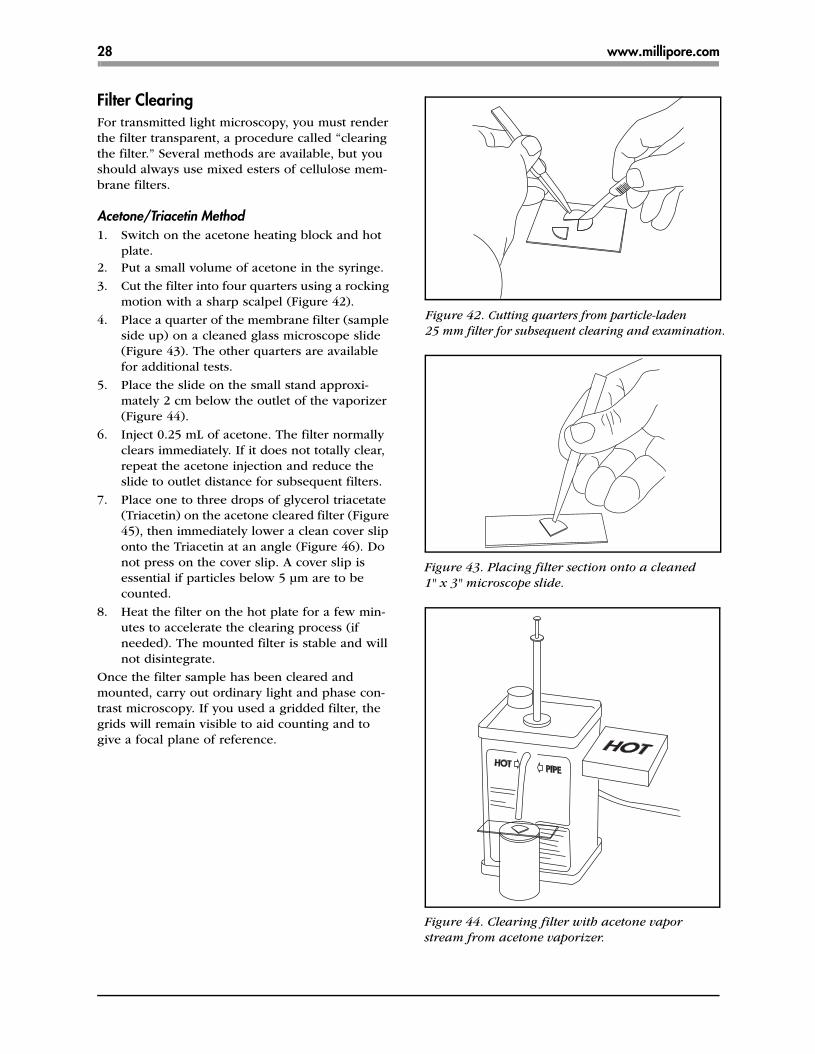
1.

Switch on the acetone heating block and hot

plate.

2.

Put a small volume of acetone in the syringe.

3.

Cut the filter into four quarters using a rocking

motion with a sharp scalpel (Figure 42).

4.

Place a quarter of the membrane filter (sample

side up) on a cleaned glass microscope slide

(Figure 43). The other quarters are available

for additional tests.

5.

Place the slide on the small stand approxi-

mately 2 cm below the outlet of the vaporizer

(Figure 44).

6.

Inject 0.25 mL of acetone. The filter normally

clears immediately. If it does not totally clear,

repeat the acetone injection and reduce the

slide to outlet distance for subsequent filters.

7.

Place one to three drops of glycerol triacetate

(Triacetin) on the acetone cleared filter (Figure

45), then immediately lower a clean cover slip

onto the Triacetin at an angle (Figure 46). Do

not press on the cover slip. A cover slip is

essential if particles below 5 µm are to be

counted.

8.

Heat the filter on the hot plate for a few min-

utes to accelerate the clearing process (if

needed). The mounted filter is stable and will

not disintegrate.

Once the filter sample has been cleared and

mounted, carry out ordinary light and phase con-

trast microscopy. If you used a gridded filter, the

grids will remain visible to aid counting and to

give a focal plane of reference.

Figure 42.

Cutting quarters from particle-laden

25 mm filter for subsequent clearing and examination.

Figure 43. Placing filter section onto a cleaned 1" x 3" microscope slide.

Figure 44. Clearing filter with acetone vapor stream from acetone vaporizer.

ADO30ch4.fm 8 Wednesday, July 1, 1998 9:53 AM

Analysis 29

Dimethylphthalate and Diethyloxylate Method

To prepare mounting medium:

1.

Dissolve Millipore aerosol analysis filter in a

1:1 solution of dimethylphthalate and diethy-

loxylate (ratio of 0.2 g filter to 1 mL of solu-

tion). You can make up large volumes of this

solution and store it out of sunlight in a stop-

pered bottle. Filter mounting medium as it is

dispensed using a solvent-resistant syringe fil-

ter unit.

2.

Place a drop of mounting medium on a freshly

cleaned glass microscope slide to mount the

membrane filter sample. For best results when

cleaning slides, rinse with filtered CFC-Free

Contact Cleaner.

3.

Use a scalpel to cut a wedge-shaped piece

from the filter with an arc length of about 1

cm. Carefully store the remaining filter. Avoid

contamination in the event a second wedge

must be cut.

4.

Transfer the wedge of filter (keep sample side

up) to the drop of mounting media using

smooth tipped filter forceps. Cover with a

cover slip. The filter becomes transparent in

about 15 minutes at room temperature.

Microscope Immersion Oil Method

Using forceps, float the filter on a film of immer-

sion oil in the cover of a plastic petri dish. Draw

the filter over the rim of the cover to remove any

excess oil and mount on the glass microscope

slide.

Equipment

When using a Millipore Fluid Contamination Anal-

ysis Kit to collect samples, you will need only the

microscope illuminator, stage micrometer and tally

counter.

A suitable microscope for particle counting should

have:

■

a binocular body

■

a mechanical stage

■

a multiple nosepiece

■

4X, 10X and 20X objectives

■

a 10X Kellner or wide-field eye piece

The Millipore XX76 100 00 microscope meets

these requirements.

Figure 45. Adding Triacetin solution to acetone cleared filter.

Figure 46. Cover slip placed at an angle over cleared filter containing Triacetin.



Measuring Eyepiece (Reticle) Calibration

Before counting and measuring particles, you must

calibrate the measuring eyepiece reticle of the

microscope using a stage micrometer. The scale is

calibrated with each objective to be used in the

counting/measuring procedure.

The stage micrometer is a glass slide with etched

graduations (Figure 47). These graduations are

accurately measured in millimeters as follows:

(a) From A to B = 1 mm (1000 µm); (b) From B to

C = 0.1 mm (100 µm); (c) From C to D = 0.01 mm

(10 µm).

1.

Swing the lowest magnification objective into

position.

2.

Remove the eyepiece from the microscope

(Figure 48) to focus the eyepiece reticle. Look

through the eyepiece with one eye and focus

the reticle while keeping the second eye open

and focused into the distance. This procedure

minimizes eye strain when particle counting.

Replace the eyepiece in the microscope.

3.

Place the stage micrometer onto the micro-

scope stage. Adjust the microscope to bring

the graduations of the stage micrometer into

sharp focus.

4.

Line up the eyepiece reticle with the stage

micrometer (Figure 49).

Assuming that the example diagram represents

what is seen when using a 4X objective (and

10X ocular), line up and calibrate the reticle

divisions. Based upon 100 divisions of this ret-

icle subtending 1050 µm on the stage

micrometer, the calibration would be:

The figure of 10.5 µm/fine division would

remain fixed for this particular combination of

microscope, 4X objective, 10X eyepiece and

reticle.

5.

Repeat the above tests for the other objectives

to be used.

6.

Make a note of these calibration factors for

future use with this microscope.

1010

100= 10.5 µm per fine division

A B CD

STAGE MICROMETER

Dimemsions

A to B = 1 mm (1000 µm)B to C = 0.1 mm (100 µm)C to D = 0.01 mm (10 µm)

Figure 47. A standard stage micrometer.

MEASURING EYEPIECE

0 20 40 60 80 100

Figure 48. A standard measuring eyepiece (reticle) containing 100 linear graduations.

1,050 µm

100 Divisions of Eyepiece subtend 1,050µm Each division of eyepiece = 10.5µm

0 20 40 60 80 100

Figure 49. Knowing the subdivisions of the stage micrometer (top), the divisions of the measuring eyepiece (bottom) may be sized from it and will remain constant at that magnification.


Analysis 31

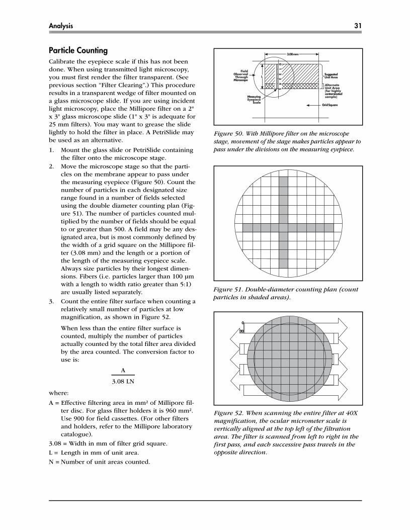
Particle Counting

Calibrate the eyepiece scale if this has not been

done. When using transmitted light microscopy,

you must first render the filter transparent. (See

previous section “Filter Clearing”.) This procedure

results in a transparent wedge of filter mounted on

a glass microscope slide. If you are using incident

light microscopy, place the Millipore filter on a 2"

x 3" glass microscope slide (1" x 3" is adequate for

25 mm filters). You may want to grease the slide

lightly to hold the filter in place. A PetriSlide may

be used as an alternative.

1.

Mount the glass slide or PetriSlide containing

the filter onto the microscope stage.

2.

Move the microscope stage so that the parti-

cles on the membrane appear to pass under

the measuring eyepiece (Figure 50). Count the

number of particles in each designated size

range found in a number of fields selected

using the double diameter counting plan (Fig-

ure 51). The number of particles counted mul-

tiplied by the number of fields should be equal

to or greater than 500. A field may be any des-

ignated area, but is most commonly defined by

the width of a grid square on the Millipore fil-

ter (3.08 mm) and the length or a portion of

the length of the measuring eyepiece scale.

Always size particles by their longest dimen-

sions. Fibers (i.e. particles larger than 100 µm

with a length to width ratio greater than 5:1)

are usually listed separately.

3.

Count the entire filter surface when counting a

relatively small number of particles at low

magnification, as shown in Figure 52.

When less than the entire filter surface is

counted, multiply the number of particles

actually counted by the total filter area divided

by the area counted. The conversion factor to

use is:

where:

A = Effective filtering area in mm² of Millipore fil-

ter disc. For glass filter holders it is 960 mm².

Use 900 for field cassettes. (For other filters

and holders, refer to the Millipore laboratory

catalogue).

3.08 =

Width in mm of filter grid square.

L =

Length in mm of unit area.

N =

Number of unit areas counted.

A

3.08 LN

10

23

45

L

3.08 mm

SuggestedUnit Area

AlternateUnit Area(for highlycontaminatedsample)

Grid Square

FieldObservedThrough

Microscope

MeasuringEyepiece

Scale

Figure 50. With Millipore filter on the microscope stage, movement of the stage makes particles appear to pass under the divisions on the measuring eyepiece.

Figure 51. Double-diameter counting plan (count particles in shaded areas).

0

20

Figure 52. When scanning the entire filter at 40X magnification, the ocular micrometer scale is vertically aligned at the top left of the filtration area. The filter is scanned from left to right in the first pass, and each successive pass travels in the opposite direction.



Particle Counting, continued

A typical counting work sheet is shown in Figure

53. Any particle size ranges may be used. These

ranges are taken from SAE ARP-598A.

When you take samples of materials such as

hydraulic fluids by means of the fluid sampler, it is

important that you remove all excess fluid from

the Millipore filter using a vacuum syringe before

the cassette is opened. (See the “On-Line Sample

Collection and Filtration” section in Chapter III for

details on the fluid sampler.) Flushing solvent

through the cassette at this point may seriously

disturb the particle distribution. It is always good

practice to prepare a blank, proceeding through all

the filtering and counting operations without intro-

ducing any sample to determine the “background”

count. This is an excellent measure of glassware,

solvent and technique cleanliness. Blank counts

should not exceed 10% of the control limits estab-

lished for the fluids being tested.

Image analysis systems and electronic counters

that automate microscopic particle counting are

now available and many component manufactur-

ers are implementing them. The primary advan-

tages of these systems are increased speed and the

elimination of error due to operator fatigue. They

do need careful calibration and careful filter prepa-

ration so that the particles lie in a single plane, as

well as good contrast between particles and back-

ground.

Millipore's Nylon Net filters are best for these auto-

mated systems because the symmetry of the nylon

net and the defined pore size make it easy to

determine particle size. The contrast between the

white screen background and the particles allows

precise calibration of the instrument before filtra-

tion. Also, the nylon material is compatible with

many solvents and can be rinsed, leaving only the

particles. Nylon net filters are available in 11µ to

180µ pore size configurations.

NOTE:

Because the nylon filters (.2-1.2µ), have a

smaller pore size and a mesh configuration,

they are not appropriate for automated par-

ticle analysis.

SCANNING ELECTRONMICROSCOPE (SEM)PARTICLE COUNTING

The techniques used to count particles in a scan-

ning electron microscope (SEM) are similar to

those used to count with a light microscope. The

operator places a membrane filter with the col-

lected sample in the SEM and counts a minimum

of 500 particles.

Using an energy dispersive X-ray analysis system,

the operator can identify the elements present in

the particles.

PARTICLE COUNT DATA SHEET

MAG.X

AREAPER

FIELD

PARTICLESIZE

RANGERECORD BELOW PARTICLES COUNTED

IN EACH RANDOM SELECTED FIELDFIELDS

COUNTED

TOTALPARTICLESCOUNTED

TOTAL AREAAREA COUNTED

PARTICLESIN

SAMPLE

PARTICLES PER

100 1.5mm2 5–15 µm 19 8 10 12 9 12 14 17 13 15 10 129 64 8256 8256

100 grid sq.

15–25 µm 9 7 8 8 13 6 8 5 7 8

12 8 11 7 8 10 5 6 8 4 20 158 5 790 790

100 grid sq.

25–50 µm 2 3 2 3 4 2 2 1 5 3

5 1 5 2 3 2 0 4 1 4 20 54 5 270 270

40 entirefilter

50–100µm 1 39 1 39 39

40 entirefilter >100µm 1 6 1 6 6

40 entirefilter fibers 1 2 1 2 2

Figure 53.

A typical counting work sheet. Any particle size range might have been used.

(A) (B) (C × D)( )D = AREA(A)(B)(C)

❏ liter

❏ 100 mL ❏ cu. ft.

✓

FLUID SAMPLE NUMBER SOURCE VOLUME DAY/MO./YR. COLLECTED BY COUNTED BY

Hydr. B. 23-N Test 100 mL 4/15/88 Peterson RHJ


Analysis 33

Sample Preparation

The preferred collection filter for counting is a

track-etched membrane with a pore size no larger

than 1/2 the size of the smallest particles to be

counted. Track-etched membranes are better

because the particles are easily visualized on the

smooth surface. The smaller pore size ensures that

the particles will be above the membrane surface,

making counting more accurate.

If using a conventional high vacuum SEM operat-

ing at high accelerating voltages, you must first

render the filter conductive. Gold or chromium

coating is preferred for optimum image resolution,

but interferes with the elemental analysis of sev-

eral elements. Carbon coating is suitable for ele-

mental analysis, but may yield poorly defined

images at high kV. If a field emission scope is

used, low kV can be used, eliminating the need for

metal coating.

Calibration

Place an approved calibration grid in the SEM. Fol-

low the manufacturer’s instructions for calibrating

the SEM prior to collecting the images for count-

ing.

Particle Size and Counting

The counting technique assumes a normal distri-

bution of particles on a collection filter. Determine

the number of fields to be counted using the num-

ber of particles per field and the number of fields

at a given magnification. As the number of parti-

cles per field decreases, the number of fields

counted increases and vice versa in order to com-

ply with the statistical needs of the normal distri-

bution.

In practice, you adjust the number of particles per

field to between 20 and 30 either by sample prepa-

ration or by decreasing the magnification. Under

such conditions, you only need to count 20 to 30

fields in order to achieve confidence levels of 90 to

95%.

In order to count the particles on a filter, you

should record at least twenty-six fields at a given

magnification. These fields cross the disc from left

to right and top to bottom. Record four additional

randomly selected fields in the four quadrants cre-

ated by the first fields. Place the number of parti-

cles counted along with the number of fields in the

formula shown below to determine the total num-

ber of particles on the collection disc.

where:

N = number of particles counted

m =

calibrated length of the micron marker in

micrometers

l

=

actual length of micron marker on the print in

cm

L = length of micrograph in cm

W = width of micrograph in cm

n = number of micrographs counted

A = filtration area of collection filter in sq. cm.

l2AN X 108

m2LWn= total particles

Recommended Magnifications for Specific Particle Sizes

In all these cases, the magnification ensures no particle to be counted is less than 2 mm

on the micrograph.

Particle Size (µm) Magnification Size of the Field (sq. cm.) No. of Fields/sq. cm.

0.261, 0.215

10000X

1.01X10

-6

9.90X10

5

0.198, 0.176, 0.142

15000X

4.5X10

-7

2.22X10

6

0.109

20000X

2.54X10

-7

3.94X10

6

0.070

35000X

8.28X10

-8

1.21X10

7

0.038

50000X

4.06X10

-8

2.46X10

7



Particle Size and Counting, continued

As an alternative method of particle sizing and

counting, you may use an image analysis software

package. The image is processed to grey levels and

the particles are sized and counted by the parame-

ters of the software or parameters set up by the

operator.

Stage automation with a software interface is avail-

able on most image analysis systems that enables

semi-automated counting and sizing of particles on

a collection filter.

PARTICLE GRAVIMETRIC ANALYSIS

Gravimetric analysis in fluids requires less skill

and equipment than microscopic particle counting.

Once the specification has been established by

weight, the gravimetric method provides a simple,

inexpensive and highly reproducible routine con-

trol measure. The ASTM recommendations for Par-

ticle Contamination in Petroleum Products (D2274)

and Aviation Fuels (D2276) recommends a gravi-

metric and color rating technique. These methods

are described in further detail in the “Air and Fluid

Monitoring Applications Guide” in Chapter VI.

Gravimetric analysis involves filtering a contami-

nated sample through a control filter and a sample

filter. In this method, you place two preweighed

filters, one on top of the other, in a single filter

holder then filter a sample. Sample contaminants

will be retained entirely by the top test filter. How-

ever, both filters are subjected to identical alter-

ations in tare weight as a result of moisture loss or

gain, sample adsorption or desorption, and other

environmental factors. Any change in weight of

the bottom (“control”) filter is then applied as a

correction to the weight of contaminant. The con-

taminant weight is determined by reweighing the

test filter and subtracting its original tare weight.

Results accurate to 0.1 mg are routinely attained

using this method.

Filter Selection

The simplest gravimetric analyses use matched

weight cassettes. Each cassette contains two Milli-

pore filters that are matched in tare weight to 0.1

mg. These cassettes are factory-assembled so that

preweighing each membrane in the field before fil-

tering the sample is unnecessary. After sampling,

the weight of the contaminant is determined sim-

ply as the difference in weight between the two

membranes.

Millipore matched weight filters, (AA) nitrocellu-

lose .8µm, are preweighed to within 0.1mg. These

are available in 47mm discs, 50 pairs per package,

and in 37 mm matched weight cassettes. See the

Millipore laboratory products catalogue or call

Technical Service for more details.


Analysis 35

Sample Preparation

The first three steps may be omitted when testing

samples from air and other gases, water and

wholly volatile solvents. All steps must be followed

with viscous liquids such as paints, hydraulic oil

and turbine fuels.

1.

Insert the aerosol adapter into stopper on the

vacuum flask (Figure 54).

2.

Remove plugs from cassette and mount the

cassette, filter side up, on the aerosol adapter

(Figure 55).

3.

Apply vacuum and introduce membrane-fil-

tered solvent through the top opening using a

solvent dispenser (Figure 56). Release vacuum.

4.

Open the cassette and transfer filters into cov-

ered glass petri dishes.

5.

Loosen the lids of the glass petri dishes and

place in an oven at 90°C for 30 minutes.

6.

Remove the dishes from the oven. With lids

ajar, allow the filter to cool and equilibrate to

ambient conditions for at least 15 minutes.

Figure 54. Placing aerosol adapter into rubber stopper, hose end down.

Figure 55. Cassette containing sample is fitted to luer slip of adapter, and stopper is fitted into filter flask (inlet plug removed).

Figure 56. Introducing flushing solvent through top opening of cassette using solvent filtering dispenser.



Result Weighing and Calculation

The procedure for determining the results of your

gravimetric analysis depends on what filter

method you used during sample collection.

Matched-Weight Filters orMatched-Weight Cassettes

1.

Reweigh both filters and record the weights.

2.

Subtract the weight of the control filter from

the weight of the test filter. The test filter will

normally be heavier than the control filter.

Negative results should be recorded as “zero”

contamination.

Typical results would be:

Control Filter Method

1.

Reweigh the filters and record the final

weights.

2.

Subtract the initial weight from the final

weight of each test filter.

3.

Determine the loss or gain in tare weight of

the control filter by appropriate subtraction. A

weight increase greater than 0.5 mg in the

control filter indicates inadequate flushing of

residual test fluid from the filter. The test

should be rerun.

4.

Apply the control filter weight change as a cor-

rection factor to the test result.

Typical results would be:

Inorganic (Noncombustible) Fraction

The inorganic fraction of the particle weight is eas-

ily determined by ashing the filter.

1.

Clean and ignite a small porcelain crucible.

2.

Place in a muffle furnace at 750°C for 20 min-

utes.

3.

Allow the crucible to cool in a desiccator and

weigh it to the nearest 0.05 mg.

4.

Repeat steps 2 and 3 until the crucible has

constant weight.

5.

Place the filter containing the contaminant res-

idue in the crucible. Wet it with ethanol and

carefully ignite the filter.

6.

Cover the crucible and place it in the muffle

furnace at 750°C for 20 minutes.

7.

Allow the crucible to cool in a desiccator and

reweigh it. As the organic sediment will have

been ignited, the final weight difference repre-

sents the inorganic particle contamination.

Test # 1 2 3

Final Weight of

Test Filter (mg)

49.20

51.30

50.80

Final Weight of

Control Filter (mg)

48.50

50.70

50.35

Results in

mg/volume filtered

0.70

0.60

0.45

Test # 1 2 3 Control

Final Weight

(mg)

49.20

51.30

50.80

49.40

Initial Weight

(mg)

48.00

49.95

49.65

49.10

Wt. (mg)

1.20

1.35

1.15

+0.30

Control

Factor

-.30

-.30

-.30

Results in

mg/volume

filtered

.90

1.05

.85


Analysis 37

PARTICLE IDENTIFICATION

The key to identifying the source of particle con-

tamination is to identify the types of particles

present. Identification almost always reveals the

source of the contamination.

Optical Microscopy

The most commonly applied technique in particle

identification is optical microscopy. It is simple to

do, inexpensive and, when done with a trained

eye, identifies the largest number of contaminant

particles. With experience, a microscopist can rec-

ognize a specific particle on sight. Physical charac-

teristics such as shape, size, color and optical

properties are used for identification. Supplemen-

tary properties include particle hardness (assessed

by pushing the microscope cover slip above the

particle with a needle) and magnetism (detected

by rotating a small magnet around the particle and

seeing if it behaves like a compass needle).

Often a microscopist can identify minute particles

that take major efforts with other analytical tech-

niques. For example, skin cells, a common con-

taminant, are easily recognized on sight. Other

methods might show the particles to be complex

organic chemicals with traces of sodium and chlo-

ride but still not lead to a useful identification.

To learn about microscopical particle identifica-

tion, McCrone Associates* has produced a Particle

Atlas and the McCrone Research Institute** teaches

courses in particle identification.

*

The Particle Atlas by McCrone and Delly

published by Ann Arbor Science Publishers.

**

McCrone Research Institute, 3620 S. Michigan

Avenue, Chicago, IL 60616.

Other Methods

If a positive identification is not possible through

optical microscopy, other methods used in particle

identification include the electron microprobe or a

scanning electron microscope (SEM) equipped

with energy dispersive X-ray analysis (EDXRA).

These methods identify the elements present in a

sample. Transmission electron microscopy (TEM)

may also identify very small particles by means of

shape and size. In addition, TEM can give selected

area electron diffraction pictures that depend on

the particle's crystal structure. By this method,

asbestos fibers such as chrysotile, amosite and cro-

cidolite (blue asbestos) can be distinguished from

each other and from other fibers. X-ray diffraction

may also be used to identify crystal structures and

hence chemical compounds. X-ray fluorescence,

like EDXRA, identifies the elements present.

Atomic absorption spectroscopy or other spectro-

scopic methods are used to determine specific

metals, especially hazardous particles in air (e.g.

beryllium or lead). Infrared spectroscopy is useful

for identifying organic compounds but, unlike the

methods above, requires a relatively large sample

size. When optical microscopy is inconclusive, you

can identify most common contaminants by one of

these methods.



COLORIMETRIC PATCH METHOD

A colorimetric patch test is a widely used proce-

dure for monitoring hydraulic fluids and aviation

fuels. In particular, it is used adjacent to aircraft or

machinery to enable an immediate decision to be

made on whether to change the fluid. Aviation fuel

is the most critical because of the number of trans-

fers the fuel will go through before it reaches its

final destination. A patch test (ASTM D3830) is

performed at each point of transfer.

The typical color of a contaminant in any given

system remains fairly constant. The greater the dis-

coloration of a filter, the greater the contamina-

tion. Increasing the sample size may increase the

sensitivity of the procedure. The Patch Test is gen-

erally applicable only to gross levels of contamina-

tion (Figure 57).Figure 57. Comparing patch obtained on filter removed from fluid sampling cassette to standard colored patches (of known contaminant levels) contained in patch test booklet.


analysis - california state university, northridgevchsc00b/466b/milliporemanual.pdfanalysis 31...

Documents