analysis and synthesis of speech using matlab€¦ · title: analysis and synthesis of speech using...

International Journal of Advancements in Research & Technology, Volume 2, Issue 5, M ay-2013 373 ISSN 2278-7763

Copyright © 2013 SciResPub. IJOART

ANALYSIS AND SYNTHESIS OF SPEECH USING MATLAB Vishv Mohan (State Topper Himachal Pradesh 2008, 2009, 2010)

B.E(Hons.) Electrical and Electronics Engineering; President-NCSTU University: Birla Institute Of Technology & Science, Pilani -333031(Rajasthan)-India

E-mail: [email protected]

ABSTRACT The interval of each sound wave has different frequency in its sub-sections. This paper has made an analysis of two matlab functions namely GenerateSpectrogram.m and MatrixToSound.m , in order to analyze and synthesis the speech signals. The first Matlab code section GenerateSpectrogram.m record the user input sound for user (more precisely from the source) defined duration and asks required parameters for computation of spectrogram and returns a matrix with frequency as rows and time as column and corresponding matrix element as amplitude of that frequency. MatrixToSound.m uses the method of additive synthesis of sound to generate sound from the user defined matrix with frequencies as its rows and time as its columns. Sound recording is an electrical or mechanical inscription of sound waves, such as spoken voice, singing, instrumental music, or sound effects. The two main classes of sound recording technology are analog recording and digital recording. Acoustic analog recording is achieved by a small microphone diaphragm that can detect changes in atmospheric pressure (acoustic sound waves) and record them as a graphic representation of the sound

waves on a medium such as a phonograph. Digital recording converts the analog sound signal picked up by the microphone to a digital form by a process of digitization, allowing it to be stored and transmitted by a wider variety of media. Digital recording stores audio as a series of binary numbers representing samples of the amplitude of the audio signal at equal time intervals, at a sample rate high enough to convey all sounds capable of being heard. The feature of analysis and synthesis of sound, is applied to create the speech with the help of matrix of elements as frequency or time domain analyzed parameters with specific amplitude.

Keywords : spectrum, synthesis, simulation, frequency, sound-waves, amplitude, wave sequence.

INTRODUCTION

The speech is an acoustic signal, hence, it is a mechanical wave that is an oscillation of pressure transmitted through solid liquid or gas and it is composed of frequencies within hearing range. Sound is a sequence of waves of pressure that propagates through compressible media such as air or water. Audible range of sound is 20 Hz to 20KHz, at standard temperature and pressure. During propagation, waves can be reflected, refracted, or attenuated by the medium.

IJOART



Recording of Sound

Sound recording is an electrical or mechanical inscription of sound waves, such as spoken voice, singing, instrumental music, or sound effects. The two main classes of sound recording technology are analog recording and digital recording. Acoustic analog recording is achieved by a small microphone diaphragm that can detect changes in atmospheric pressure (acoustic sound waves) and record them as a graphic representation of the sound waves on a medium such as a phonograph (in which a stylus senses grooves on a record). In magnetic tape recording, the sound waves vibrate the microphone diaphragm and are converted into a varying electric current, which is then converted to a varying magnetic field by an electromagnet, which makes a representation of the sound as magnetized areas on a plastic tape with a magnetic coating on it.

Digital recording converts the analog sound signal picked up by the microphone to a digital form by a process of digitization, allowing it to be stored and transmitted by a wider variety of media. Digital recording stores audio as a series of binary numbers representing samples of the amplitude of the audio signal at equal time intervals, at a sample rate high enough to convey all sounds capable of being heard. Digital recordings are considered higher quality than analog recordings not necessarily because they have higher

fidelity (wider frequency response or dynamic range), but because the digital format can prevent much loss of quality found in analog recording due to noise and electromagnetic interference in playback, and mechanical deterioration or damage to the storage medium. A digital audio signal must be reconverted to analog form during playback before it is applied to a loudspeaker or earphones.

Analysis of Sound Signal

The long-term frequency analysis of speech signals yields good information about the overall frequency spectrum of the signal, but no information about the temporal location of those frequencies. Since speech is a very dynamic signal with a time-varying spectrum, it is often insightful to look at frequency spectra of short sections of the speech signal. Long-term frequency analysis The frequency response of a system is defined as the discrete-time Fourier transform (DTFT) of the system's impulse response h[n]:

Similarly, for a sequence x[n], its long-term frequency spectrum is defined as the DTFT of the Sequence

Theoretically, we must know the sequence x[n] for all values of n (from n=-∞ until n=∞) in order to compute its frequency spectrum. Fortunately, all terms where x[n] = 0 do not matter in the sum, and therefore an equivalent expression for the sequence's spectrum is

IJOART



Here we've assumed that the sequence starts at 0 and is N samples long. This tells us that we can apply the DTFT only to all of

the non-zero samples of x[n], and still obtain the sequence's true spectrum X (ω). But what is the correct mathematical expression to compute the spectrum over a short section of

the sequence, that is, over only part of the non-zero samples of the sequence? Window sequence It turns out that the mathematically correct way to do that is to multiply the sequence x[n] by a ‘window sequence’ w[n] that is non-zero only for n=0… L-1, where L, the length of the window, is smaller than the length N of the sequence x[n]:

Then we compute the spectrum of the windowed sequence xw [n] as usual

The following figure illustrates how a window sequence w[n] is applied to the sequence x[n]:

As the figure shows, the windowed sequence is shorter in length than the original sequence. So we can further truncate the DTFT of the windowed sequence:

Using this windowing technique, we can select any section of arbitrary length of the input sequence x[n] by choosing the length and location of the window accordingly. The window sequence w[n] affect the short-term frequency spectrum.

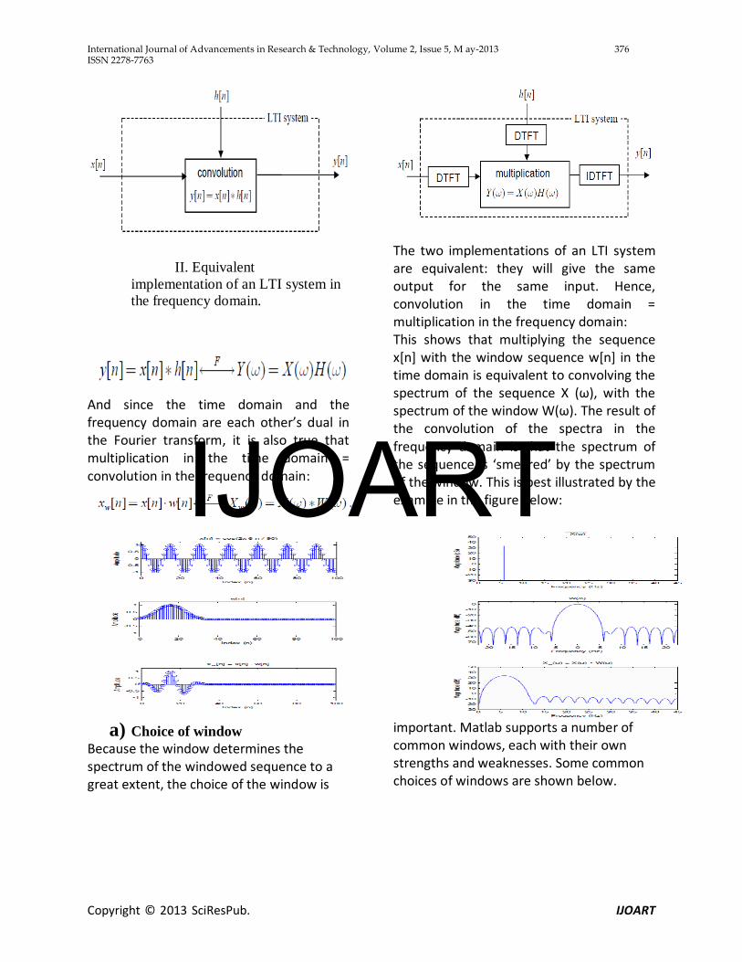
Effect of the window To answer that question, we need to introduce an important property of the Fourier transform. The diagram below illustrates the property graphically: I. Implementation of an LTI system in the time domain.

IJOART



II. Equivalent implementation of an LTI system in the frequency domain.

The two implementations of an LTI system are equivalent: they will give the same output for the same input. Hence, convolution in the time domain = multiplication in the frequency domain:

And since the time domain and the frequency domain are each other’s dual in the Fourier transform, it is also true that multiplication in the time domain = convolution in the frequency domain:

This shows that multiplying the sequence x[n] with the window sequence w[n] in the time domain is equivalent to convolving the spectrum of the sequence X (ω), with the spectrum of the window W(ω). The result of the convolution of the spectra in the frequency domain is that the spectrum of the sequence is ‘smeared’ by the spectrum of the window. This is best illustrated by the example in the figure below:

a) Choice of window Because the window determines the spectrum of the windowed sequence to a great extent, the choice of the window is

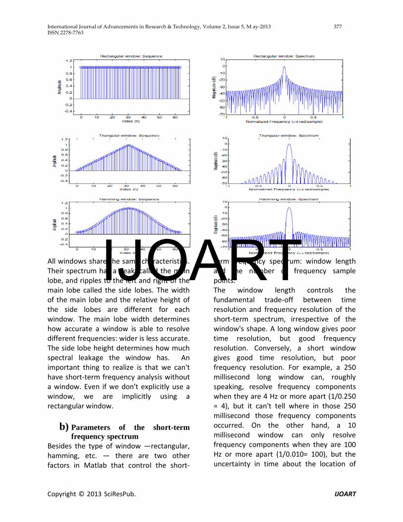
important. Matlab supports a number of common windows, each with their own strengths and weaknesses. Some common choices of windows are shown below.

IJOART



All windows share the same characteristics. Their spectrum has a peak, called the main lobe, and ripples to the left and right of the main lobe called the side lobes. The width of the main lobe and the relative height of the side lobes are different for each window. The main lobe width determines how accurate a window is able to resolve different frequencies: wider is less accurate. The side lobe height determines how much spectral leakage the window has. An important thing to realize is that we can't have short-term frequency analysis without a window. Even if we don't explicitly use a window, we are implicitly using a rectangular window.

b) Parameters of the short-term frequency spectrum

Besides the type of window —rectangular, hamming, etc. — there are two other factors in Matlab that control the short-

term frequency spectrum: window length and the number of frequency sample points. The window length controls the fundamental trade-off between time resolution and frequency resolution of the short-term spectrum, irrespective of the window's shape. A long window gives poor time resolution, but good frequency resolution. Conversely, a short window gives good time resolution, but poor frequency resolution. For example, a 250 millisecond long window can, roughly speaking, resolve frequency components when they are 4 Hz or more apart (1/0.250 = 4), but it can't tell where in those 250 millisecond those frequency components occurred. On the other hand, a 10 millisecond window can only resolve frequency components when they are 100 Hz or more apart (1/0.010= 100), but the uncertainty in time about the location of

IJOART



those frequencies is only 10 millisecond. The result of short-term spectral analysis using a long window is referred to as a narrowband spectrum (because a long window has a narrow main lobe), and the result of short-term spectral analysis using a short window is called a wideband spectrum. In short-term spectral analysis of speech, the window length is often chosen with respect to the fundamental period of

the speech signal, i.e., the duration of one period of the fundamental frequency. A common choice for the window length is either less than 1 times the fundamental period, or greater than 2-3 times the fundamental period. Examples of narrowband and wideband short-term spectral analysis of speech are given in the figures below:

The other factor controlling the short-term spectrum in Matlab is the number of points at which the frequency spectrum H (ω) is evaluated. The number of points is usually equal to the length of the window. Sometimes a greater number of points is chosen to obtain a smoother looking spectrum. Evaluating H (ω) at fewer points than the window length is possible, but very rare.

c) Time-frequency domain: Spectrogram

An important use of short-term spectral analysis is the short-time Fourier transform or spectrogram of a signal. The spectrogram of a sequence is constructed by computing the short term spectrum of a windowed version of the sequence, then shifting the window over to a new location and repeating this process until the entire sequence has been analyzed. The whole process is illustrated in the figure below:

Together, these short-term spectra (bottom row) make up the spectrogram, and are typically shown in a two-dimensional plot,

where the horizontal axis is time, the vertical axis is frequency, and magnitude is the color or intensity of the plot. For example:

IJOART



The appearance of the spectrogram is controlled by a third parameter: window overlap. Window overlap determines how much the window is shifted between repeated computations of the short term spectrum. Common choices for window overlap are 50% or 75% of the window length. For example, if the window length is 200 samples and window overlap is 50%, the window would be shifted over 100 samples between each short-term spectrum. In the case that the overlap was 75%, the window would be shifted over 50 samples. The choice of window overlap depends on the application. When a temporally smooth spectrogram is desirable, window overlap should be 75% or more. When computation should be at a minimum, no overlap or 50% overlap are good choices. If computation is not an issue, you could even compute a new short-term spectrum for every sample of the sequence. In that case, window overlap = window length – 1, and the window would only shift

1 sample between the spectra. But doing so is wasteful when analyzing speech signals, because the spectrum of speech does not change at such a high rate. It is more practical to compute a new spectrum every 20-50 millisecond, since that is the rate at which the speech spectrum changes. In a wideband spectrogram (i.e., using a window shorter than the fundamental period), the fundamental frequency of the speech signal resolves in time. That means that you can't really tell what the fundamental frequency is by looking at the frequency axis, but you can see energy fluctuations at the rate of the fundamental frequency along the time axis. In a narrowband Spectrogram (i.e., using a window 2-3 times the fundamental period), the fundamental frequency resolves in frequency, i.e., you can see it as an energy peak along the frequency axis.

GenerateTimeVsFreq.m

1) Duration=input('Enter the time in seconds for which you want to record:');

2) samplingRate=input('Enter what sampling rate is required of audio 8000 or 22050: ');

3) timeResolution=input('Enter the time resolution desired in millisecond: ');

4) frequencyResolution=input('enter the frequency resolution required: '); 5) usedWindowLength =ceil(samplingRate/frequencyResolution); 6) recObj = audiorecorder(samplingRate,8,1); 7) disp('Start speaking.') 8) recordblocking(recObj,Duration); 9) disp('End of Recording.'); 10) % Play back the recording. 11) play(recObj); 12) % Store data in double-precision array. 13) myRecordingData = getaudiodata(recObj); 14) figure(1) 15) plot (myRecordingData); 16) % No of Data points= samplingRate*Duration; 17) % No of columns in spectrogram=(duration*1000)/timeResolution; 18) % =duration*frequencyResolution; 19) actualWindowLength= ceil((samplingRate*timeResolution)/1000); 20) overlapLength= usedWindowLength -actualWindowLength +4;

IJOART



21) % Plot the spectrogram 22) S

=spectrogram(myRecordingData,usedWindowLength,overlapLength,samplingRate-1,samplingRate,'yaxis');

23) [ar ac]=size(S); 24) S1=imresize(S,[ar (Duration*1000)/timeResolution]); 25) AbsoluteMagnitude=abs(S1); 26) figure(2) 27) spectrogram(myRecordingData,256,200,256,samplingRate-1,'yaxis'); 28) TimeInterval=input('Enter the time interval in terms of multiple

of time resolution to see the frequencies present at that moment:'); 29) figure(3) 30) plot(AbsoluteMagnitude(:,timeInterval));

Synthesis of Sound

There are many methods of sound synthesis. Jeff Pressing in "Synthesizer Performance and Real-Time Techniques" gives this list of approaches to sound synthesis, namely Additive synthesis, Subtractive synthesis, frequency modulation synthesis ,sampling ,composite synthesis ,phase distortion , wave shaping ,Re-synthesis ,granular synthesis ,linear predictive coding ,direct digital synthesis ,wave sequencing ,vector synthesis ,physical modeling.

We are using additive synthesis to synthesize the sound from matrix having rows as different frequencies and columns as time intervals.

a) Additive Synthesis

Additive synthesis is a sound synthesis technique that creates timbre by adding sine waves together. In music, timbre also known as tone color or tone quality from psychoacoustics(i.e. scientific study of sound perception) , is the quality of a musical note or sound or tone that distinguishes different types of sound production, such as voices and musical instruments, string instruments, wind instruments, and percussion instruments

Additive synthesis generates sound by adding the output of multiple sine wave generators. Harmonic additive synthesis is closely related to the concept of a Fourier series which is a way of expressing a periodic function as the sum of sinusoidal functions with frequencies equal to integer multiples of a common fundamental frequency. These sinusoids are called harmonics, overtones, or generally, partials. In general, a Fourier series contains an infinite number of sinusoidal components, with no upper limit to the frequency of the sinusoidal functions and includes a DC component (one with frequency of 0 Hz). Frequencies outside of the human audible range can be omitted in additive synthesis. As a result only a finite number of sinusoidal terms with frequencies that lie within the audible range are modeled in additive synthesis.

b) Harmonic form

The simplest harmonic additive synthesis can be mathematically expressed as:

where ,y(t) is the synthesis output, , , and are the amplitude, frequency, and the phase offset of the th harmonic partial of a total of harmonic partials, and is the fundamental frequency of the

IJOART



waveform and the frequency of the musical note.

c) Time-dependent amplitudes

More generally, the amplitude of each harmonic can be prescribed as

a function of time, , in which case the synthesis output is

d) Matlab Code

MatrixToSound.m

1) % FUNCTION TO PLAY SOUND FROM THE MATRIX 2) samplingRate= input('please enter the sampling rate used: '); 3) timeResolution= input('Please enter the time resolution in milliseconds: '); 4) matrix= input('please enter the matrix for conversion to sound'); 5) lowerThreshold= input('Please enter the lower threshold value below which the

matrix element should be neglected( a number between 0 and 255: '); 6) time=0:1/samplingRate:(timeResolution/1000); 7) [mrows mcolumn]= size(matrix); 8) count=0; 9) [timerow NoOfComponents]= size(time); 10) SineVector=zeros(1,NoOfComponents); 11) InitialSoundMatrix=zeros(NoOfComponents,mcolumn); 12) for j=1:mcolumn 13) for i=1:mrows 14) if(matrix(i,j)>lowerThreshold) 15) t=matrix(i,j)*sin(2*pi*time*i); 16) count=count+1; 17) SineVector=SineVector+t; 18) end 19) end 20) InitialSoundMatrix(:,j)=(SineVector’) 21) end 22) SoundMatrix=InitialSoundMatrix./(255*count); 23) [SMRow SMColumn]=size(SoundMatrix); 24) SoundColumn=reshape(SoundMatrix,SMRow*SMColumn,1); 25) soundsc(SoundColumn,samplingRate);

Conclusion

The spectra of the sound corresponding to time can be computed using the GenerateTimeVsFrequency.m matlab file and its result matches approximately with that of specgramdemo function of the matlab. Additive synthesis of sound can be simulated with the help of the matlab file created MatrixToSound.m. It approximates the actual sound.

Acknowledgement My research paper is dedicated to my parents Sh. Vasu Dev Sharma, Lecturer Biology at Government Senior Secondary School Bilaspur Himachal Pradesh(India) and Smt. Bandna Sharma; T.G.T Mathematics at Sarswati Vidya Mandir Bilaspur Himachal Pradesh(India) whose blessing and wishes made me capable to complete this paper more effectively and efficiently.

IJOART



References

(a) Textbooks [1] Oppenheim, A.V., and R.W. Schafer, Discrete-Time Signal Processing, Prentice-Hall, Englewood Cliffs, NJ, 1989, pp.713-718.

[2] Rabiner, L.R., and R.W. Schafer, Digital Processing of Speech Signals, Prentice-Hall, Englewood Cliffs, NJ, 1978.

(b) Websources

1) http://www.mathworks.in/matlabcentral/fileexchange/index?utf8=%E2%9C%93&term=spectrogram

2) http://en.wikipedia.org/wiki/Additive_synthesis#Time-dependent_amplitudes

3) http://isdl.ee.washington.edu/people/stevenschimmel/sphsc503/

http://hyperphysics.phy-astr.gsu.edu/hbase/audio/synth.html

By: Er. Vishv Mohan, s/o Sh. Vasu Dev Sharma

State Topper Himachal Pradesh 2008, 2009, 2010. B.E(Hons.) Electrical & Electronics Engineering, BITS-Pilani_(Rajasthan)-333031_India. [email protected]

IJOART

http://www.mathworks.in/matlabcentral/fileexchange/index?utf8=%E2%9C%93&term=spectrogram



http://en.wikipedia.org/wiki/Additive_synthesis#Time-dependent_amplitudes

http://en.wikipedia.org/wiki/Additive_synthesis#Time-dependent_amplitudes

http://isdl.ee.washington.edu/people/stevenschimmel/sphsc503/

http://isdl.ee.washington.edu/people/stevenschimmel/sphsc503/



analysis and synthesis of speech using matlab€¦ · title: analysis and synthesis of speech using...

Documents