analysis and simulation of wireless ofdm communicaions a
TRANSCRIPT

ANALYSIS AND SIMULATION OF WIRELESS OFDM COMMUNICAIONS
A Thesis
Presented to the
Faculty of
San Diego State University
In Partial Fulfillment
of the Requirements for the Degree
Master of Science in Applied Mathematics
with a Concentration in
Mathematical Theory of Communication Systems
by
Steven Charles Hemple
Summer 2012


iii
Copyright © 2012
by
Steven Charles Hemple

iv
DEDICATION
Dedicated to my patient and loving wife.

v
A mathematician is a device for turning coffee into theorems.
– Paul Erdos

vi
ABSTRACT OF THE THESIS
Analysis and Simulation of Wireless OFDM Communicationsby
Steven Charles HempleMaster of Science in Applied Mathematics with a Concentration in Mathematical Theory of
Communication SystemsSan Diego State University, 2012
The increase in the number of wireless devices and the requirement for higher datarates places an increasing demand on bandwidth. This necessitates the need forcommunication systems with increased throughput and capacity. Multiple input multipleoutput orthogonal frequency division multiplexing (MIMO-OFDM) is one way to meet thisneed. OFDM is used in many wireless communication devices and offers high spectralefficiency and resilience to multipath channel effects. Though OFDM is sensitive tosynchronization errors, it makes the task of channel equalization simple. MIMO makes use ofmultiple antennas to increase throughput without increasing transmitter power or bandwidth.
This thesis presents an introduction to the multipath fading channel and describes anappropriate channel model. Several modulation schemes arepresented that are often used inconjunction with OFDM . Mathematical definitions and analysis of OFDM are given alongwith a discrete implementation common to modern communication systems. Synchronizationerrors are described mathematically and simulated, as wellas techniques to estimate andcorrect those errors at the receiver. Lastly, space time coding, spatial multiplexing, andbeamforming are presented as techniques used in (MIMO).

vii
TABLE OF CONTENTS
PAGE
ABSTRACT .. . . . . . . . . . . . . . . . . . . . . . . . . . . . . . . . . . . . . . . . . . . . .. . . . . . . . . . . . . . . . . . . . . . . . . . . . . . . . . . . . . . vi
LIST OF TABLES.. . . . . . . . . . . . . . . . . . . . . . . . . . . . . . . . . . . . . . .. . . . . . . . . . . . . . . . . . . . . . . . . . . . . . . . . . . . . . x
LIST OF FIGURES .. . . . . . . . . . . . . . . . . . . . . . . . . . . . . . . . . . . . . .. . . . . . . . . . . . . . . . . . . . . . . . . . . . . . . . . . . . . xi
ACKNOWLEDGEMENTS .. . . . . . . . . . . . . . . . . . . . . . . . . . . . . . . . . . . .. . . . . . . . . . . . . . . . . . . . . . . . . . . . . . . xv
CHAPTER
1 INTRODUCTION .. . . . . . . . . . . . . . . . . . . . . . . . . . . . . . . . . . . . . .. . . . . . . . . . . . . . . . . . . . . . . . . . . . . . 1
1.1 History . . . . . . . . . . . . . . . . . . . . . . . . . . . . . . . . . . . . . . . . .. . . . . . . . . . . . . . . . . . . . . . . . . . . . . . . . . . 1
1.2 Objective. . . . . . . . . . . . . . . . . . . . . . . . . . . . . . . . . . . . . . .. . . . . . . . . . . . . . . . . . . . . . . . . . . . . . . . . . 2
1.3 Preview of Chapters . . . . . . . . . . . . . . . . . . . . . . . . . . . . . . . .. . . . . . . . . . . . . . . . . . . . . . . . . . . . . 2
2 THE CHANNEL . . . . . . . . . . . . . . . . . . . . . . . . . . . . . . . . . . . . . . . . .. . . . . . . . . . . . . . . . . . . . . . . . . . . . . . 3
2.1 Propagation Mechanisms . . . . . . . . . . . . . . . . . . . . . . . . . . .. . . . . . . . . . . . . . . . . . . . . . . . . . . . 3
2.1.1 Large Scale Effects . . . . . . . . . . . . . . . . . . . . . . . . . . . . .. . . . . . . . . . . . . . . . . . . . . . . . . . . 3
2.1.2 Mid-Scale Effects . . . . . . . . . . . . . . . . . . . . . . . . . . . . . .. . . . . . . . . . . . . . . . . . . . . . . . . . . . 6
2.1.3 Small Scale Effects . . . . . . . . . . . . . . . . . . . . . . . . . . . . .. . . . . . . . . . . . . . . . . . . . . . . . . . . 6
2.2 Electromagnetic Model . . . . . . . . . . . . . . . . . . . . . . . . . . . .. . . . . . . . . . . . . . . . . . . . . . . . . . . . . 8
2.3 Impulse Response Model . . . . . . . . . . . . . . . . . . . . . . . . . . . . .. . . . . . . . . . . . . . . . . . . . . . . . . . 14
2.4 Frequency Domain Channel Model . . . . . . . . . . . . . . . . . . . . . .. . . . . . . . . . . . . . . . . . . . . . 18
2.5 Implementation of Channel Model . . . . . . . . . . . . . . . . . . . . .. . . . . . . . . . . . . . . . . . . . . . . . 21
3 MODULATION TECHNIQUES.. . . . . . . . . . . . . . . . . . . . . . . . . . . . . .. . . . . . . . . . . . . . . . . . . . . . . 27
3.1 Amplitude Modulation . . . . . . . . . . . . . . . . . . . . . . . . . . . . .. . . . . . . . . . . . . . . . . . . . . . . . . . . . . 27
3.1.1 Double Side Band Amplitude Modulation . . . . . . . . . . . . . .. . . . . . . . . . . . . . . . . 27
3.1.2 Double Side Band Suppressed Carrier. . . . . . . . . . . . . . . . .. . . . . . . . . . . . . . . . . . . 29
3.1.3 Single Side Band . . . . . . . . . . . . . . . . . . . . . . . . . . . . . . . . .. . . . . . . . . . . . . . . . . . . . . . . . . 29
3.1.4 Hilbert Transform. . . . . . . . . . . . . . . . . . . . . . . . . . . . . .. . . . . . . . . . . . . . . . . . . . . . . . . . . . 31
3.2 Pulse Amplitude Modulation . . . . . . . . . . . . . . . . . . . . . . . .. . . . . . . . . . . . . . . . . . . . . . . . . . . 34
3.3 Phase Shift Keying/Quadrature Phase Shift Keying . . . . .. . . . . . . . . . . . . . . . . . . . . . 36
3.4 Quadrature Amplitude Modulation. . . . . . . . . . . . . . . . . . .. . . . . . . . . . . . . . . . . . . . . . . . . . 38
4 ORTHOGONAL FREQUENCY DIVISION MULTIPLEXING .. . . . . . . . . . . .. . . . . . . 45

viii
4.1 Single Carrier Systems. . . . . . . . . . . . . . . . . . . . . . . . . . . . .. . . . . . . . . . . . . . . . . . . . . . . . . . . . . 45
4.2 Multicarrier System .. . . . . . . . . . . . . . . . . . . . . . . . . . . . .. . . . . . . . . . . . . . . . . . . . . . . . . . . . . . . 46
4.3 Mathematical Description of OFDM.. . . . . . . . . . . . . . . . . .. . . . . . . . . . . . . . . . . . . . . . . . 46
4.3.1 Modulation . . . . . . . . . . . . . . . . . . . . . . . . . . . . . . . . . . . .. . . . . . . . . . . . . . . . . . . . . . . . . . . . . 49
4.3.2 Demodulation of AWGN Channel . . . . . . . . . . . . . . . . . . . . . . .. . . . . . . . . . . . . . . . . 50
4.3.3 Demodulation of Delay Dispersive Channel . . . . . . . . . . .. . . . . . . . . . . . . . . . . . 50
4.4 Implementing OFDM .. . . . . . . . . . . . . . . . . . . . . . . . . . . . . . .. . . . . . . . . . . . . . . . . . . . . . . . . . . 52
5 SYNCHRONIZATION ERRORS AND ESTIMATIONS .. . . . . . . . . . . . . . . . .. . . . . . . . . 59
5.1 Syncronization Errors . . . . . . . . . . . . . . . . . . . . . . . . . . . .. . . . . . . . . . . . . . . . . . . . . . . . . . . . . . . 60
5.1.1 Frequency Offset . . . . . . . . . . . . . . . . . . . . . . . . . . . . . . .. . . . . . . . . . . . . . . . . . . . . . . . . . . 60
5.1.2 Sampling Clock Offset . . . . . . . . . . . . . . . . . . . . . . . . . . . .. . . . . . . . . . . . . . . . . . . . . . . . 65
5.1.3 Frame Timing Offset . . . . . . . . . . . . . . . . . . . . . . . . . . . . .. . . . . . . . . . . . . . . . . . . . . . . . . 73
5.2 Synchronization Error Estimation . . . . . . . . . . . . . . . . . .. . . . . . . . . . . . . . . . . . . . . . . . . . . . 87
5.2.1 Preamble Structure of IEEE802.11a . . . . . . . . . . . . . . . .. . . . . . . . . . . . . . . . . . . . . . 87
5.2.2 OFDM Frame Timing Estimation . . . . . . . . . . . . . . . . . . . . .. . . . . . . . . . . . . . . . . . . 91
5.2.3 Frequency Offset Estimation . . . . . . . . . . . . . . . . . . . . .. . . . . . . . . . . . . . . . . . . . . . . . . 94
5.2.4 Symbol Timing Estimation. . . . . . . . . . . . . . . . . . . . . . . .. . . . . . . . . . . . . . . . . . . . . . . . 105
5.2.5 Channel Estimation . . . . . . . . . . . . . . . . . . . . . . . . . . . . . .. . . . . . . . . . . . . . . . . . . . . . . . . . 107
5.2.6 Residual Frequency Offset . . . . . . . . . . . . . . . . . . . . . . . .. . . . . . . . . . . . . . . . . . . . . . . . 108
6 MULTIPLE INPUT MULTIPLE OUTPUT .. . . . . . . . . . . . . . . . . . . . . .. . . . . . . . . . . . . . . . . . . 112
6.1 Space Time Coding . . . . . . . . . . . . . . . . . . . . . . . . . . . . . . . . . .. . . . . . . . . . . . . . . . . . . . . . . . . . . 112
6.1.1 Space Time Trellis Codes . . . . . . . . . . . . . . . . . . . . . . . . . .. . . . . . . . . . . . . . . . . . . . . . . 113
6.1.2 Space Time Block Codes . . . . . . . . . . . . . . . . . . . . . . . . . . . . .. . . . . . . . . . . . . . . . . . . . . 115
6.2 Viterbi Decoder . . . . . . . . . . . . . . . . . . . . . . . . . . . . . . . . . .. . . . . . . . . . . . . . . . . . . . . . . . . . . . . . . 119
6.2.1 Hard Decision Viterbi Decoder . . . . . . . . . . . . . . . . . . . .. . . . . . . . . . . . . . . . . . . . . . . 119
6.2.2 Soft Decision Viterbi Decoding . . . . . . . . . . . . . . . . . . .. . . . . . . . . . . . . . . . . . . . . . . . 121
6.3 Spatial Division Multiplexing . . . . . . . . . . . . . . . . . . . . .. . . . . . . . . . . . . . . . . . . . . . . . . . . . . 121
6.4 Beamforming . . . . . . . . . . . . . . . . . . . . . . . . . . . . . . . . . . . . . .. . . . . . . . . . . . . . . . . . . . . . . . . . . . . . 125
6.5 Channel Estimation . . . . . . . . . . . . . . . . . . . . . . . . . . . . . . . .. . . . . . . . . . . . . . . . . . . . . . . . . . . . . 125
7 CONCLUSION .. . . . . . . . . . . . . . . . . . . . . . . . . . . . . . . . . . . . . . . . .. . . . . . . . . . . . . . . . . . . . . . . . . . . . . . 130
BIBLIOGRAPHY .. . . . . . . . . . . . . . . . . . . . . . . . . . . . . . . . . . . . . . . . .. . . . . . . . . . . . . . . . . . . . . . . . . . . . . . . . . . . . 132

ix
APPENDICES
A MATLAB CODE FOR CHANNEL MODELING .. . . . . . . . . . . . . . . . . . . . . . .. . . . . . . . . . . 135
B MATLAB CODE FOR MODULATION .. . . . . . . . . . . . . . . . . . . . . . . . . . .. . . . . . . . . . . . . . . . . 146
C MATLAB CODE FOR OFDM .. . . . . . . . . . . . . . . . . . . . . . . . . . . . . . . . .. . . . . . . . . . . . . . . . . . . . . . 159
D MATLAB CODE FOR SYNCHRONIZATION .. . . . . . . . . . . . . . . . . . . . . . .. . . . . . . . . . . . . . 168
E MATLAB CODE FOR PREAMBLE AND SYNCHRONIZATION ER-ROR ESTIMATION .. . . . . . . . . . . . . . . . . . . . . . . . . . . . . . . . . . . . .. . . . . . . . . . . . . . . . . . . . . . . . . . . . . 187
F CORRELATION .. . . . . . . . . . . . . . . . . . . . . . . . . . . . . . . . . . . . . . . . .. . . . . . . . . . . . . . . . . . . . . . . . . . . . . 208
G PHASE LOCK LOOP .. . . . . . . . . . . . . . . . . . . . . . . . . . . . . . . . . . . . .. . . . . . . . . . . . . . . . . . . . . . . . . . . 210
H MATLAB CODE FOR PLL . . . . . . . . . . . . . . . . . . . . . . . . . . . . . . . . . . .. . . . . . . . . . . . . . . . . . . . . . . . 223

x
LIST OF TABLES
PAGE
Table 2.1. Relationship Between Channel Parameters and Model Parameters . . . . . . . . . . . . . . 20
Table 6.1. Alamouti Transmission Scheme . . . . . . . . . . . . . . . .. . . . . . . . . . . . . . . . . . . . . . . . . . . . . . . . . . . 116
Table 6.2. Encoder Transition and Inputs . . . . . . . . . . . . . . . .. . . . . . . . . . . . . . . . . . . . . . . . . . . . . . . . . . . . . 120
Table 6.3. Soft Decision Viterbi Decoder . . . . . . . . . . . . . . . .. . . . . . . . . . . . . . . . . . . . . . . . . . . . . . . . . . . . . 121

xi
LIST OF FIGURES
PAGE
Figure 2.1. Free space model. . . . . . . . . . . . . . . . . . . . . . . . . . .. . . . . . . . . . . . . . . . . . . . . . . . . . . . . . . . . . . . . . . 4
Figure 2.2. Free space path loss model for large and small distances. . . . . . . . . . . . . . . . . . . . . . . . 5
Figure 2.3. Doppler shift as a function of speed and angle relative to the transmit antenna. 7
Figure 2.4. Static reflection from wall and line of sight paths. . . . . . . . . . . . . . . . . . . . . . . . . . . . . . . . 8
Figure 2.5. Same phase. . . . . . . . . . . . . . . . . . . . . . . . . . . . . . . .. . . . . . . . . . . . . . . . . . . . . . . . . . . . . . . . . . . . . . . . . 9
Figure 2.6.λ4
difference. . . . . . . . . . . . . . . . . . . . . . . . . . . . . . . . . . . . . . . . .. . . . . . . . . . . . . . . . . . . . . . . . . . . . . . . 10
Figure 2.7.λ2
difference. . . . . . . . . . . . . . . . . . . . . . . . . . . . . . . . . . . . . . . . .. . . . . . . . . . . . . . . . . . . . . . . . . . . . . . . 11
Figure 2.8. Isotropic antennas with Rx antenna movement.. . .. . . . . . . . . . . . . . . . . . . . . . . . . . . . . . . 12
Figure 2.9. Fixed isotropic antennas with two paths. . . . . . .. . . . . . . . . . . . . . . . . . . . . . . . . . . . . . . . . . . 12
Figure 2.10. Fixed transmit antenna and moving receive antenna with two paths. . . . . . . . . . 13
Figure 2.11. Channel transfer function with three paths andW = 1GHz, θk =0 andak = 1 for k = 1, 2, 3, 4, 5. . . . . . . . . . . . . . . . . . . . . . . . . . . . . . . . . . . . . . . . . . . . . . . . . . .. . . 16
Figure 2.12. Delay power spectrum. . . . . . . . . . . . . . . . . . . . . .. . . . . . . . . . . . . . . . . . . . . . . . . . . . . . . . . . . . . 19
Figure 2.13. The frequency domain model. . . . . . . . . . . . . . . . .. . . . . . . . . . . . . . . . . . . . . . . . . . . . . . . . . . . 21
Figure 2.14. Output of noise shaping filter. . . . . . . . . . . . . . .. . . . . . . . . . . . . . . . . . . . . . . . . . . . . . . . . . . . . 22
Figure 2.15. Output of Hilbert transform. . . . . . . . . . . . . . . .. . . . . . . . . . . . . . . . . . . . . . . . . . . . . . . . . . . . . . 23
Figure 2.16. Simulated transfer function. . . . . . . . . . . . . . .. . . . . . . . . . . . . . . . . . . . . . . . . . . . . . . . . . . . . . . 24
Figure 2.17. Simulated impulse response. . . . . . . . . . . . . . . .. . . . . . . . . . . . . . . . . . . . . . . . . . . . . . . . . . . . . 25
Figure 2.18. PDF of 3000 simulations. . . . . . . . . . . . . . . . . . . .. . . . . . . . . . . . . . . . . . . . . . . . . . . . . . . . . . . . . 26
Figure 3.1. Time series and frequency spectrum of message and carrier signal. . . . . . . . . . . . . 28
Figure 3.2. Time series and frequency spectrum of modulatedsignal. . . . . . . . . . . . . . . . . . . . . . . 29
Figure 3.3. Time series and frequency spectrum of DSB-SC. . . . .. . . . . . . . . . . . . . . . . . . . . . . . . . . 30
Figure 3.4. Frequency spectrum of Hilbert transform. . . . . .. . . . . . . . . . . . . . . . . . . . . . . . . . . . . . . . . . 33
Figure 3.5. Frequency spectrum of modulated SSB. . . . . . . . . . .. . . . . . . . . . . . . . . . . . . . . . . . . . . . . . . 33
Figure 3.6. PAM-4 constellation. . . . . . . . . . . . . . . . . . . . . . .. . . . . . . . . . . . . . . . . . . . . . . . . . . . . . . . . . . . . . . . 34
Figure 3.7. PAM-4 signal with Gray coding. . . . . . . . . . . . . . . .. . . . . . . . . . . . . . . . . . . . . . . . . . . . . . . . . . 35
Figure 3.8. Gray coding scheme for BPSK.. . . . . . . . . . . . . . . . . .. . . . . . . . . . . . . . . . . . . . . . . . . . . . . . . . . 39
Figure 3.9. Gray coding scheme for QPSK. . . . . . . . . . . . . . . . . .. . . . . . . . . . . . . . . . . . . . . . . . . . . . . . . . . 40

xii
Figure 3.10. Constellation diagram for 16-QAM. . . . . . . . . . . .. . . . . . . . . . . . . . . . . . . . . . . . . . . . . . . . . 41
Figure 3.11. Gray coding scheme for 16-QAM. . . . . . . . . . . . . . .. . . . . . . . . . . . . . . . . . . . . . . . . . . . . . . . 43
Figure 3.12. Receiver block diagram for M-QAM. . . . . . . . . . . . .. . . . . . . . . . . . . . . . . . . . . . . . . . . . . . . 44
Figure 4.1. Single carrier system block diagram. . . . . . . . . .. . . . . . . . . . . . . . . . . . . . . . . . . . . . . . . . . . . . 46
Figure 4.2. Single carrier system showing frequency response, power delayspectrum and symbols. . . . . . . . . . . . . . . . . . . . . . . . . . . . . . . . .. . . . . . . . . . . . . . . . . . . . . . . . . . . . . . . . . 47
Figure 4.3. Multiple carrier system block diagram. . . . . . . .. . . . . . . . . . . . . . . . . . . . . . . . . . . . . . . . . . . 47
Figure 4.4. Multiple carrier system showing frequency response, power delayspectrum and symbols. . . . . . . . . . . . . . . . . . . . . . . . . . . . . . . . .. . . . . . . . . . . . . . . . . . . . . . . . . . . . . . . . . 48
Figure 4.5. Cyclic prefix. . . . . . . . . . . . . . . . . . . . . . . . . . . . . . .. . . . . . . . . . . . . . . . . . . . . . . . . . . . . . . . . . . . . . . . 51
Figure 4.6. Real part of IDFT output. . . . . . . . . . . . . . . . . . . . . .. . . . . . . . . . . . . . . . . . . . . . . . . . . . . . . . . . . . 54
Figure 4.7. Imaginary part of IDFT output. . . . . . . . . . . . . . . .. . . . . . . . . . . . . . . . . . . . . . . . . . . . . . . . . . . . 55
Figure 4.8. IFFT as a complex signal generator. . . . . . . . . . . .. . . . . . . . . . . . . . . . . . . . . . . . . . . . . . . . . . . 56
Figure 4.9. FFT as a complex signal demodulator. . . . . . . . . . .. . . . . . . . . . . . . . . . . . . . . . . . . . . . . . . . . 57
Figure 5.1. Synchronization blocks in OFDM receiver. . . . . .. . . . . . . . . . . . . . . . . . . . . . . . . . . . . . . . . 59
Figure 5.2. Effects of normalized carrier frequency offsetǫ = 0.05 andSNR=20dB for 120 simulations. . . . . . . . . . . . . . . . . . . . . . . . . . .. . . . . . . . . . . . . . . . . . . . . . . . . . . . 62
Figure 5.3. Effects of normalized carrier frequency offsetǫ = 0.05 andSNR=20dB on the constellation for 120 OFDM Symbols. . . . . . . . .. . . . . . . . . . . . . . . . . . 63
Figure 5.4. Effects of normalized carrier frequency offsetǫ = 0.05 andSNR=20dB on the spectrum for 120 OFDM Symbols. . . . . . . . . . . . . .. . . . . . . . . . . . . . . . . 64
Figure 5.5. ICI coefficients forǫ = 0.5, 0.1, 0.05, 0.025. . . . . . . . . . . . . . . . . . . . . . . . . . . . . . . . . . . . . . 65
Figure 5.6. Power of ICI. . . . . . . . . . . . . . . . . . . . . . . . . . . . . . . .. . . . . . . . . . . . . . . . . . . . . . . . . . . . . . . . . . . . . . . 66
Figure 5.7. Carrier-to-interference power ratio.. . . . . . . .. . . . . . . . . . . . . . . . . . . . . . . . . . . . . . . . . . . . . . . 67
Figure 5.8. Time series with1% sample clock offset. . . . . . . . . . . . . . . . . . . . . . . . . . . . . . . . . .. . . . . . . 68
Figure 5.9. Magnitude of attenuation and phase of 1% sampling period offset. . . . . . . . . . . . . 70
Figure 5.10. Effects of sample clock offset on spectrum. . . .. . . . . . . . . . . . . . . . . . . . . . . . . . . . . . . . . 71
Figure 5.11. Effects of sample clock offset on constellation. . . . . . . . . . . . . . . . . . . . . . . . . . . . . . . . . 72
Figure 5.12. ICI power. . . . . . . . . . . . . . . . . . . . . . . . . . . . . . . . .. . . . . . . . . . . . . . . . . . . . . . . . . . . . . . . . . . . . . . . . 74
Figure 5.13. Signal to ICI power ratio. . . . . . . . . . . . . . . . . . . .. . . . . . . . . . . . . . . . . . . . . . . . . . . . . . . . . . . . . 75
Figure 5.14. Effects of symbol timing offset ofζ = 8 for Nfft = 64. . . . . . . . . . . . . . . . . . . . . . . . 77
Figure 5.15. Effects of symbol timing offset ofζ = 8 for Nfft = 256. . . . . . . . . . . . . . . . . . . . . . 78
Figure 5.16. Possible locations for frame start position. .. . . . . . . . . . . . . . . . . . . . . . . . . . . . . . . . . . . . 79

xiii
Figure 5.17. Effects of symbol timing offset ofζ = 8 for Nfft = 64 with cyclicprefix and ideal channel. . . . . . . . . . . . . . . . . . . . . . . . . . . . . . .. . . . . . . . . . . . . . . . . . . . . . . . . . . . . . . . . 80
Figure 5.18. Effects of symbol timing offset ofζ = 8 for Nfft = 64 with cyclicprefix and multipath channel. . . . . . . . . . . . . . . . . . . . . . . . . . .. . . . . . . . . . . . . . . . . . . . . . . . . . . . . . . . 81
Figure 5.19. Effects of symbol timing offset ofζ = 8 for Nfft = 64 with cyclicprefix and multipath channel. . . . . . . . . . . . . . . . . . . . . . . . . . .. . . . . . . . . . . . . . . . . . . . . . . . . . . . . . . . 82
Figure 5.20. Effects of symbol timing offset ofζ = 8 for Nfft = 64 with nocyclic prefix and ideal channel. . . . . . . . . . . . . . . . . . . . . . . . .. . . . . . . . . . . . . . . . . . . . . . . . . . . . . . . . 84
Figure 5.21. Effects of symbol timing offset ofζ = 8 for Nfft = 256 with nocyclic prefix and ideal channel. . . . . . . . . . . . . . . . . . . . . . . . .. . . . . . . . . . . . . . . . . . . . . . . . . . . . . . . . 85
Figure 5.22. Power of ICI, ISI, and total interference forNfft = 64. . . . . . . . . . . . . . . . . . . . . . . . 86
Figure 5.23. Spectrum of short training symbols. . . . . . . . . .. . . . . . . . . . . . . . . . . . . . . . . . . . . . . . . . . . . 88
Figure 5.24. Time series of short training symbols. . . . . . . .. . . . . . . . . . . . . . . . . . . . . . . . . . . . . . . . . . . 89
Figure 5.25. Spectrum of long training symbols. . . . . . . . . . .. . . . . . . . . . . . . . . . . . . . . . . . . . . . . . . . . . . 90
Figure 5.26. Time series of long training symbols. . . . . . . . .. . . . . . . . . . . . . . . . . . . . . . . . . . . . . . . . . . . 92
Figure 5.27. Time series of preamble. . . . . . . . . . . . . . . . . . . .. . . . . . . . . . . . . . . . . . . . . . . . . . . . . . . . . . . . . . 93
Figure 5.28. Delay and correlate algorithm. . . . . . . . . . . . . .. . . . . . . . . . . . . . . . . . . . . . . . . . . . . . . . . . . . . 93
Figure 5.29. Output of the cross-correlator, the auto-correlator, and the thresh-old detector. . . . . . . . . . . . . . . . . . . . . . . . . . . . . . . . . . . . . . . .. . . . . . . . . . . . . . . . . . . . . . . . . . . . . . . . . . . . . 95
Figure 5.30. Received signal with 50 samples prepended. . . . .. . . . . . . . . . . . . . . . . . . . . . . . . . . . . . . 96
Figure 5.31. Time series of preamble with SNR≈ 7dB and frequency offset 200kHz. . . . . 97
Figure 5.32. Output of the cross-correlator, the auto-correlator, and the thresh-old detector with SNR≈ 7dB and frequency offset 200kHz. . . . . . . . . . . . . . . . . . . . . . . .. 98
Figure 5.33. Frequency estimation algorithm. . . . . . . . . . . .. . . . . . . . . . . . . . . . . . . . . . . . . . . . . . . . . . . . . 100
Figure 5.34. Estimated phase. . . . . . . . . . . . . . . . . . . . . . . . . .. . . . . . . . . . . . . . . . . . . . . . . . . . . . . . . . . . . . . . . . 101
Figure 5.35. Time series with and without frequency offset correction. . . . . . . . . . . . . . . . . . . . . . 102
Figure 5.36. Output of phase detector and loop filter. . . . . . .. . . . . . . . . . . . . . . . . . . . . . . . . . . . . . . . . . 103
Figure 5.37. Accumulated phase and VCO output. . . . . . . . . . . . .. . . . . . . . . . . . . . . . . . . . . . . . . . . . . . . 104
Figure 5.38. Constellation with and without frequency offset correction. . . . . . . . . . . . . . . . . . . . 105
Figure 5.39. Cross-correlation of long training symbol. . . .. . . . . . . . . . . . . . . . . . . . . . . . . . . . . . . . . . 106
Figure 5.40. Effects of multipath channel on received constellation. . . . . . . . . . . . . . . . . . . . . . . . . 107
Figure 5.41. Channel estimation. . . . . . . . . . . . . . . . . . . . . . . .. . . . . . . . . . . . . . . . . . . . . . . . . . . . . . . . . . . . . . . 109
Figure 5.42. Received constellation after channel correction. . . . . . . . . . . . . . . . . . . . . . . . . . . . . . . . 110
Figure 5.43. Scrambler used to generate psuedo-binary pilot sequence. . . . . . . . . . . . . . . . . . . . . 110

xiv
Figure 5.44. Residual frequency tracking. . . . . . . . . . . . . . . .. . . . . . . . . . . . . . . . . . . . . . . . . . . . . . . . . . . . . 111
Figure 6.1. Rate1/2 convolutional encoder with constraint length 7. . . . . . . . . .. . . . . . . . . . . . . . 113
Figure 6.2. Four state convolutional encoder. . . . . . . . . . . .. . . . . . . . . . . . . . . . . . . . . . . . . . . . . . . . . . . . . . 114
Figure 6.3. State diagram for encoder in Figure 6.2. . . . . . . .. . . . . . . . . . . . . . . . . . . . . . . . . . . . . . . . . . 114
Figure 6.4. Trellis diagram for convolutional encoder in Figure 6.2. . . . . . . . . . . . . . . . . . . . . . . . . 114
Figure 6.5. Alamouti for two transmit antennas.. . . . . . . . . .. . . . . . . . . . . . . . . . . . . . . . . . . . . . . . . . . . . . 115
Figure 6.6. Alamouti for one receive antenna. . . . . . . . . . . . .. . . . . . . . . . . . . . . . . . . . . . . . . . . . . . . . . . . . 115
Figure 6.7. Channel for two transmit antennas and one receiveantenna. . . . . . . . . . . . . . . . . . . . 116
Figure 6.8. Channel for two transmit antennas and two receiveantennas. . . . . . . . . . . . . . . . . . . 118
Figure 6.9. Viterbi decoding algorithm. . . . . . . . . . . . . . . . .. . . . . . . . . . . . . . . . . . . . . . . . . . . . . . . . . . . . . . . 120
Figure 6.10. Input/output relationship for 3 bit quantizer.. . . . . . . . . . . . . . . . . . . . . . . . . . . . . . . . . . . . 122
Figure 6.11. Comparison of hard and soft Viterbi decoding.. .. . . . . . . . . . . . . . . . . . . . . . . . . . . . . . . 123
Figure 6.12. D-BLAST and V-BLAST layered transmission scheme. . . . . . . . . . . . . . . . . . . . . . . 124
Figure 6.13. Directing coverage area to intended users using beamforming. . . . . . . . . . . . . . . . 126
Figure 6.14. Three isotropic antenna configuration. . . . . . .. . . . . . . . . . . . . . . . . . . . . . . . . . . . . . . . . . . . 126
Figure 6.15. Signal strength for (a) three antennas, distance 10, and relativephase delay 10, (b) three antennas, distance 10, and relative phase delay40, (c) five antennas, distance 2, and relative phase delay 25, and (d) fiveantennas, distance 5, and relative phase delay 40. . . . . . . . .. . . . . . . . . . . . . . . . . . . . . . . . . . . . 127
Figure 6.16. MIMO channel. . . . . . . . . . . . . . . . . . . . . . . . . . . . .. . . . . . . . . . . . . . . . . . . . . . . . . . . . . . . . . . . . . . 128
Figure 6.17. Alternate transmission of long preamble. . . . .. . . . . . . . . . . . . . . . . . . . . . . . . . . . . . . . . . . 129
Figure 6.18. Alternating even and odd frequencies. . . . . . . .. . . . . . . . . . . . . . . . . . . . . . . . . . . . . . . . . . . 129
Figure G.1. Basic phase lock loop. . . . . . . . . . . . . . . . . . . . . . . .. . . . . . . . . . . . . . . . . . . . . . . . . . . . . . . . . . . . . 211
Figure G.2. Phase lock loop. . . . . . . . . . . . . . . . . . . . . . . . . . . .. . . . . . . . . . . . . . . . . . . . . . . . . . . . . . . . . . . . . . . . 211
Figure G.3. Dampened spring mass system. . . . . . . . . . . . . . . . .. . . . . . . . . . . . . . . . . . . . . . . . . . . . . . . . . . 212
Figure G.4. Undamped system. . . . . . . . . . . . . . . . . . . . . . . . . . .. . . . . . . . . . . . . . . . . . . . . . . . . . . . . . . . . . . . . . 213
Figure G.5. Damped system. . . . . . . . . . . . . . . . . . . . . . . . . . . . .. . . . . . . . . . . . . . . . . . . . . . . . . . . . . . . . . . . . . . 214
Figure G.6. Proportional control. . . . . . . . . . . . . . . . . . . . . .. . . . . . . . . . . . . . . . . . . . . . . . . . . . . . . . . . . . . . . . . 215
Figure G.7. Integral control. . . . . . . . . . . . . . . . . . . . . . . . . .. . . . . . . . . . . . . . . . . . . . . . . . . . . . . . . . . . . . . . . . . . 216
Figure G.8. Proportional and integral control. . . . . . . . . . .. . . . . . . . . . . . . . . . . . . . . . . . . . . . . . . . . . . . . . 217
Figure G.9. Input to PLL. . . . . . . . . . . . . . . . . . . . . . . . . . . . . . .. . . . . . . . . . . . . . . . . . . . . . . . . . . . . . . . . . . . . . . . 220
Figure G.10. Input and output phases to PLL, loop filter, and phase detector. . . . . . . . . . . . . . . 221
Figure G.11. PLL input and output time series. . . . . . . . . . . . .. . . . . . . . . . . . . . . . . . . . . . . . . . . . . . . . . . 222

xv
ACKNOWLEDGEMENTS
I would like to thank Professors Stefan Hui, Roxana Smarandache and Fredric J.
Harris.

1
CHAPTER 1
INTRODUCTION
The year 2010 saw global mobile data usage increase by almostthreefold [4]. This
increased data usage is from the rise in the number of consumer electronic devices that rely on
wireless standards such as IEEE802.11 (Wi-Fi), IEEE802.16(WiMAX), and cell phones in
particular multi-function smart phones [27]. The rising number of devices that require high
data rates is placing increasing demands on bandwidth. One of the ways these challenges are
being met is with the use of orthogonal frequency division multiplexing (OFDM). OFDM is
not only spectrally efficient but resilient to the effects ofthe multipath wireless channel.
Another technique being used is multiple input multiple output (MIMO). MIMO has already
been incorporated into the IEEE802.11n, IEEE802.16e, and 4G cellular wireless standards.
The introduction of MIMO into these standards make possiblethe increased data throughput
and range required by many devices without increases in transmit power or bandwidth.
1.1 HISTORY
The first use of a digital wireless electronic communicationsystem was the wireless
telegraph. This was also the first use of multiple antennas which aided in the success of
transatlantic wireless communications. Since that time digital communications has become
the de facto standard in modern communications. Though manystandards exist for the
different types of wireless digital communications we are most interested in those concerning
wireless local area networks (WLAN) also referred to as Wi-Fi. These are described by the
IEEE802.11 standard.
The first IEEE802.11 standard was released in 1997 and offered data rates of 1 and 2
Mbits/s [11]. In 1999, amendment a was released and increased the data rates to 54M bits/s
and introduced the use of OFDM as the modulation scheme [12].The inclusion of OFDM
helped to achieve the higher data rate and also increased coverage area. 2003 saw the release
of the g amendment. This amendment also included OFDM but where 802.11a achieved 54
Mbits/s at the 5GHz the g standard achieves this rate at the lower 2.4GHz [14]. The latest
release, amendment n, also uses OFDM and operates at both 2.4and 5 GHz but achieves
considerably higher data rates of up to 600 Mbits/s with the inclusion of MIMO [15]. MIMO
allows the use of multiple spatial streams to increase throughput, coverage, and even user
capacity.

2
1.2 OBJECTIVE
The goal for this thesis is to give the reader an introductorylook into OFDM. Within
this goal, the three main topics presented are channel modeling, OFDM and synchronization,
and MIMO. It is important to give an accurate representationof the channel since it has the
largest impact on the parameters of any communication system. A mathematical description
of OFDM is given as well as the discrete implementation basedon the IEEE802.11 standard.
The reader will become familiar with the synchronization difficulties that arise in
implementing OFDM as well as the estimation and correction of those errors. An introduction
to MIMO is also presented based on the IEEE802.11n standard.The reader is presented with
space time coding, spatial multiplexing, and beamforming.
1.3 PREVIEW OF CHAPTERS
Chapter 2 gives a detailed description of the wireless multipath channel. Three
different models are discussed to highlight the different aspects of the channel. The last model
is accompanied by a MATLAB simulation based on the material presented in [21]. Chapter 3
is a review of the different modulation schemes used in digital communications. Though some
are not used as often in conjunction with OFDM, they are the basis for schemes that are.
Chapter 4 covers OFDM. Mathematical definitions of both continuous and discrete versions
are given along with a comparison to single carrier systems.The discrete implementation of
OFDM given uses the IEEE802.11a/g as a guide. Chapter 5 presents synchronization errors
common to OFDM systems. Mathematical descriptions and simulations of the different errors
are presented and analyzed. The second half of the chapter discusses techniques to estimate
and correct those errors in the receiver. Chapter 6 discussesthe advantages and challenges of
MIMO. Three main topics are discussed: space time coding, spatial multiplexing, and
beamforming. The appendices contain some background information that might be useful to
the reader such as correlation and an in depth look into phaselock loops. Also included are
MATLAB scripts used in this thesis.

3
CHAPTER 2
THE CHANNEL
The success of any communication system model resides with the accurate
representation of the channel. This is especially so with the wireless channel. Effects which
are non-existent or negligible in a wired communication system can render a wireless channel
unusable unless measures are taken to counteract them.
Variations in channel statistics, called propagation mechanisms, can be placed into
three categories: small, mid, and large scale effects [10].These categories are described by
the effect that interact with the system based on the separation distance between the transmit
(Tx) and receive (Rx) antennas relative to the radio frequency (RF) wavelength. Each of these
variations can be modeled precisely with the electromagnetic wave equations but as we will
see later, their complexity make them impractical as usefulmodels.
In this chapter we will look at the electromagnetic wave model as a way to gain insight
into the interferences in a wireless channel. This will leadus into the impulse response model.
In this model the channel is considered to be a linear time invariant filter making simulation
more achievable. Several methods have been proposed as to the technique to generate the
impulse response but we will consider one that is presented in [21].
2.1 PROPAGATION M ECHANISMS
Here we describe the effects that the channel has on the wireless channel. Two types
of propagation mechanisms are described here: large and small scale. These describe how the
channel affects the propagation of the electromagnetic wave for large and small distances
relative to the wavelength.
2.1.1 Large Scale EffectsLarge scale propagation effects are those which occur at large distances, many times
the RF carrier wavelength. Two types of large scale propagation effects are path loss and
shadowing. Path loss is the simplest propagation mechanismto model as it is the decrease in
signal power as a function of distance. Consider the simplestcase where the transmitter and
receiver are isotropic antennas and are separated by a distancer in a free space environment
as shown in Figure 2.1.
We assume the antenna radiates isotropically and thus the power is the same along the
sphere with the transmit antenna at the origin. It is easy to see that the power will decrease as

4
Figure 2.1. Free space model.
the reciprocal of the distance squared. The path lossFL can be described, in positive terms, by
FL =
(
4πr
λ
)2
=
(
4πrf
c
)2
, (2.1)
where wavelengthλ, frequencyf , and the speed of lightc are related byλ = c/f [24]. Free
space path loss is usually expressed in decibels,
FL = 20 log10
(
4πrf
c
)
. (2.2)
This model does have is its limitations however. Note that asr → 0 the free space loss
FL → ∞ which clearly can not happen since this indicates an increase in power, greater than
that transmitted. Figure 2.2 demonstrates this anomaly with f = 900MHz and distance in
meters.
The second large scale propagation model is shadowing. Thiseffect is caused by path
obstructions like buildings, vegetation, etc. Though models exist that use information from
geographical information systems (GIS) databases, they are used mainly for cell tower
placement[16]. Because of the difficulty in accounting for the voluminous causes of
shadowing and the distances involved, we will not consider this effect in our model.

5
0 50 100−80
−70
−60
−50
−40
−30
−20
−10
0
10
Free Space Path Lossas a Function of Distance
Distance [m]
Mag
nitu
de [d
B]
0 0.02 0.04−10
0
10
20
30
40
50
60
70
80
90
100
Free Space Path Loss Modelas a Function of Distance
For Small Distances.
Distance [m]
Mag
nitu
de [d
B]
Figure 2.2. Free space path loss model for large and small distances.

6
2.1.2 Mid-Scale EffectsMid scale effects are variations in the channel for same antenna separation distance
and same local area. This effect can be seen when two sets of antennas are in the same room
with the same distance but with drastically different attenuations in the different paths. These
effects will also be excluded from our model except were theycontribute to small scale
effects.
2.1.3 Small Scale EffectsThese are the effects that we will devote our attention to andderive models for mostly
because for indoor applications they are the dominant effect. The first small scale effect we
consider is Doppler shift. This is caused by either the transmitter or the receiver antenna
moving but for convenience we assume that the transmit is fixed, without loss of generality.
The movement of the antenna will have an effect on the frequency of the transmitted signal.
We saw previously that wavelength and frequency are relatedby the speed of light,λ = f/c,
for stationary antennas. The change in frequency or Dopplershift is dependent on the velocity
of the antenna,v, and the angle between the line of sight and the direction of motion,θ, [26],
∆f =v
cf cos (θ) . (2.3)
Equation 2.3 does not take into account relativistic properties such as time dilation and so the
equality is an approximation. Figure 2.3 shows the Doppler shift as a function ofv andθ.
Note that for|θ| = π/2, there is no Doppler shift which is what we would expect if thereceive
antenna is moving perpendicular, or transverse, to the transmit antenna.
The second small scale effect is multipath fading. This propagation mechanism is the
result of the constructive and destructive interference from the multiple paths taken between
Tx and Rx antenna. These paths can be the line of sight (LOS) or reflections from structures
or terrain. Figure 2.4 describes the most basic scenario with two paths, the LOS and a perfect
reflection off a wall.
The received signal is a superposition of the multiple paths. For our analysis we will
assume (as is the case for practical systems) that the transmitted signal is a sinusoid. With this
in mind, the delay in each path imposes a difference in phase from the LOS path.
Figures 2.5- 2.7 show the effect the two paths with phase differences (in terms of the
wavelength) have on the received sinusoid.
The first graph shows that when the two paths have the same phase the sinusoids add
constructively. The second shows that, while a1/4 wavelength difference increases the
amplitude, the phase of the received sinusoid has shifted. Clearly, with a1/2 wavelength
difference the two sinusoids cancel out and the received sinusoid is collapsed.

7
020
4060
80100
−pi−pi/2
0pi/2
pi
−400
−300
−200
−100
0
100
200
300
Speed [m/s]
Doppler Shift as a Function of Speed and Angle Relative to Transmit Antenna
Angle [Radians]
Dop
pler
Shi
ft [H
z]
Figure 2.3. Doppler shift as a function of speed and angle relative to the transmitantenna.

8
Figure 2.4. Static reflection from wall and line of sight paths.
Consider the IEEE 802.11 standard which has carrier frequencies of2.4GHz or5GHz
and wavelengths
λ =c
f=
2.99× 10⁸m/s2.4× 109Hz
= 0.125meters (2.4)
(2.5)
and
λ =c
f=
2.99× 10⁸m/s5× 109Hz
= 0.06meters. (2.6)
Thus, we have a complete cancellation of the received sinusoid if two paths have a phase
difference of0.0625 meters for a2.4GHz system or0.03 meters for a5GHz system. Unlike
the large scale effects, these occur at ranges well within the parameters for an indoor system,
which is why we will consider multipath fading in our model.
2.2 ELECTROMAGNETIC M ODEL
It should be understood that any signal transmitted in a wireless channel is the
propagation of an electromagnetic wave, and to that end, an electro magnetic model would
seem to be the ideal method to model the channel. As we will see, the complex nature of
indoor multipath fading renders this model impractical to implement in simulation for any
practical system, due to the large number of paths. However,analyzing the channel with this
model can aid in a better understanding of the nature of smallscale propagation mechanisms
and to this effect we will consider the development of the electromagnetic model.
Let us start with the simplest of models: two isotropic antennas in a free space
environment as shown in Figure 2.1. The electric field at a point ~d can be expressed as
E(
f, t, ~d)
=αs(θ, ψ, f)e
2πjf(
t− r
c
)
r, (2.7)

9
−1
−0.5
0
0.5
1Two Waveforms With Phase Difference Full Wavelength.
−2
−1.5
−1
−0.5
0
0.5
1
1.5
2The Received Waveform
Figure 2.5. Same phase.

10
−1
−0.5
0
0.5
1Two Waveforms With Phase Difference 1/4 Wavelength.
−2
−1.5
−1
−0.5
0
0.5
1
1.5
2The Received Waveform
Figure 2.6. λ4
difference.
where~d represents the point(r, θ, ψ) for distancer and horizontal and vertical anglesψ, θ and
the termαs(θ, ψ, f) is the complex function describing the radiation pattern ofthe
transmitting antenna[7]. The magnitude ofαs accounts for the antenna loss and the phase
accounts for the change in phase due to the antenna and is dependent not only on horizontal
and vertical angles but frequency as well. From equation 2.7we can see a phase shift in the
electric field offr/c and is a result of the delay ofr/c from the traveling sinusoid. Ther in
the denominator is to be expected as we saw earlier a decreasein power by1/r2. We will
define the product of the Tx and Rx antenna patterns asα(θ, ψ, f). Thus the received
waveform is
yf (t) =α(θ, ψ, f)e
2πjf(
t− r
c
)
r. (2.8)
Equation 2.7 describes the scenario when both Tx and Rx antennas are fixed. We now
consider the case when the receive antenna is moving and the transmit antenna is fixed as
shown in Figure 2.8.

11
−1
−0.5
0
0.5
1Two Waveforms With Phase Difference 1/2 Wavelength.
−2
−1.5
−1
−0.5
0
0.5
1
1.5
2The Received Waveform
Figure 2.7. λ2
difference.
The point(r(t), θ, ψ) at which we observe the energy in the received waveform is now
a function of time and can be described by
E(
f, t, ~d(t))
=α(θ, ψ, f)e
2πj
[
f(
1 − v
c
)
t− fr0c
]
r0 + vt. (2.9)
As expected, there is a Doppler shift of−fv/c caused by the movement. This
introduces a time variance and means that we can not use the easier linear time invariant
model (LTI) unless some assumptions are made [7].
The next case is where we account for the multipath caused by areflection from a wall
as seen in Figure 2.9. It was stated earlier that it was difficult to simulate multipath with the
electromagnetic model and for that reason we will only consider two paths: the LOS and one
reflection.
Because both antenna are fixed, the received waveform can be described by
yf (t) =α(θ, ψ, f)e2πjf(t − r
c)
r− α(θ, ψ, f)e
2πjf
(
t − 2d− r
c
)
2d− r, (2.10)

12
Figure 2.8. Isotropic antennas with Rx antenna movement.
Figure 2.9. Fixed isotropic antennas with two paths.

13
whered is the distance from the transmitter to the wall andr is the distance between
transmitter and receiver. The first term is what we saw in equation 2.7 and accounts for the
LOS path while the second term is the reflected path and is negative for that reason1. The first
term has a phase shift of−fr/c, while the second has a phase shift offr/c. Even with the
antennas fixed, we can see a difference in phase between the paths.
If we now allow the receive antenna to move toward the transmit antenna with
constant velocity as seen in Figure 2.10, we have the received waveform as
yf (t) =α(θ, ψ, f)e
2πjf
(
t − r0 − vt
c
)
r0 − vt− α(θ, ψ, f)e
2πjf
(
t − r0 + vt
c
)
r0 + vt(2.11)
where the distance between antennas is(r0 − vt) and the distance between Tx and the wall is
r0.
Figure 2.10. Fixed transmit antenna and moving receive antenna withtwo paths.
Because the antenna separation is decreasing, the magnitudeof the LOS path is
increasing as1/(r0 − vt). Likewise, the distance of the reflected path is increasing,so the
magnitude is decreasing as1/(r0 + vt). The sinusoids for the LOS path has frequency
f(1− v/c) and the reflected path has frequencyf(1 + v/c). Since the received waveform is
the addition of the two waveforms, the received waveform hasfrequencyfv/c.
These last few models only account for movement along the LOSpath for perfect
reflections, and only two paths. If we wish to implement this model to analyze, for example,
an indoor wireless communication system, it would prove very challenging. In the next
section we look at a different way to model the channel and after making a few reasonable
assumptions, we will see a more implementable simulation.
1A more detailed explanation involving ray tracing can be found in [7] and [26].

14
2.3 IMPULSE RESPONSEM ODEL
In the impulse response model, we consider the channel as a filter. This means that our
task is to find the impulse response of the channel. We would like to use a linear time
invariant (LTI) filter model, but as we saw previously, thereis a time varying aspect. We,
therefore, need a few additional assumptions.
First, we consider the path amplitudes. The electromagnetic model described earlier
can accurately model each path amplitude, but the complexity in solving such equations is not
useful in simulation. Two statistical models presented in [24] are Rician and Rayleigh
probability density function (pdf). The Rician pdf describes path amplitudes when there is a
dominant non-fading path such as LOS. The Rayleigh pdf describes the case when many
paths exist but no LOS. In addition, we will assume that thereare a fixed number of paths, that
the time delay between paths are equidistant [16], and that the phases are of a uniform
distribution.
There are some aspects of these assumptions that need further discussion. It is not
difficult to see that the number of paths must be fixed for the purpose of simulation. In a more
robust approach we may consider that the number of paths is random and that there arrival is
in groups with arrival times having a Poisson distribution.The groups themselves can be
modeled with a Rayleigh pdf. This model would have a differentinstantaneous power delay
profile [16]. Both models still have a generally exponential decaying power delay profile.
The general linear time varying complex filter used to describe the wireless channel
impulse response is
h(t, τ) =
N(τ)∑
k=1
βk(t)δ [τ − τk(t)] ejθk(t) (2.12)
wheret is the observation time of the impulse,τ is the application time of the impulse,N(τ)
is the number of multipath components,βk(t) is the random time varying path amplitude,
τk(t) is the arrival time andθk(t) is the phase [17]. This model will describe the channel
completely and the received signal is just the convolution of the signals(t) with h(t, τ) and
the addition of noise. We stated earlier that an LTI model wasdesirable, thus we need the
phase, amplitude, and delay to not be time dependent. To justify this, we note that the symbol
time for 802.11a is 4µs on a2.4GHz RF [12]. This means that the wavelengthλ = 0.125
meters, but the waveform propagates from the antenna at2.99× 108 m/s. Since we are
considering indoor uses only, it is unlikely that the channel parameters will change during
transmission for some length of time.
We can define the LTI complex impulse response for the channelas
h(τ) =N∑
k=1
βkδ (τ − τk) ejθk (2.13)

15
and the received signal is then
y(t) =
∫ ∞
−∞s(t)h(τ − τ)dτ + n(t), (2.14)
wheren(t) is the noise in the channel to be discussed later. We can also describe the channel
by its transfer function
H(f) =
∫ ∞
−∞h(τ)e(−j2πfτ)dτ
=
∫ ∞
−∞
N∑
k=1
βkδ (τ − τk) e(jθk)e(−j2πfτ)dτ
=N∑
k=1
βke−j(2πfτk−θk). (2.15)
Earlier, we assumed for our simulation thatτk = (k − 1)T whereT = 1/W andW is the
bandwidth of the signal.
To illustrate the implementation of the transfer function in simulation, consider the
example whereW = 1GHz and there are five paths present. Figure 2.11 shows the transfer
function withθk = 0 andβk = 1 for k = 1, 2, 3, 4, 5. Even though this example is very
simple, compared to an indoor wireless channel commonly seen and channel parameters were
chosen for ease, fading can still be seen in the channel.
We now turn our attention to the channel parametersβ, θ, andτ and their distributions.
The length of the path the signal travels from transmitter toreceiver has a significant impact
on the phase of the received signal. Thus, any change in the position of the receive antenna (or
transmitter antenna) results in a change in the phase. We assumed earlier that the number of
paths was fixed but made no other restrictions. If we also assume a large number of paths, the
distribution of the phases along the paths generally followa uniform distribution on the
interval [0, 2π)2[17]. This assumption is based on the short wavelengths and small indoor area
that we are considering.
The path amplitude distribution depends on the presence of aLOS path. For this
simulation we will assume that the LOS component is present and therefore use the Rician
model. This model assumes that in addition to the LOS path there are a large number of
independent smaller (in magnitude) paths. It is important to point out that the Rayleigh and
Rician models do not approximate the channel for an individual situation very well. They do
approximate the channel when all physical situations are averaged[7]. The Rician pdf is
2A more detailed explanation and alternative distributionscan be found in [17]

16
−0.5 −0.4 −0.3 −0.2 −0.1 0 0.1 0.2 0.3 0.4 0.5−40
−30
−20
−10
0
10
20
Channel Transfer Function forβ
k=1 and θ
k=0
Normalized Frequency f/fsym [Hz]
Mag
nitu
de2 [d
B]
Figure 2.11. Channel transfer function with three paths andW = 1GHz, θk = 0 andak = 1 for k = 1, 2, 3, 4, 5.

17
described by
PR(r) =r
ψ0
e
[
−(r2+ρ2)2ψ0
]
I0
(
rρ
ψ0
)
(2.16)
whereψ0 is the power of the scattered rays,ρ2 is the normalized power of the direct (LOS)
ray, andI0(x) is the modified Bessel function of the first kind. A very important characteristic
of the channel is the Rician K factor,
K =β2i,max
ρ0 − β2i,max
, (2.17)
which is the ratio of the powers of the dominant path to the scattered paths. This ratio
specifies the depth of the fades. For local areas a large K value has shallow fades because the
dominant path’s power has a greater magnitude than the scattered paths and thus is not
affected by the lower magnitude interference.
Before discussing the channel parameterτ , the specific application of this model must
be established. The channel we are simulating is continuousbut the implementation of any
simulation is discrete and therefore imposes restrictionson the delay. This means we must
sample the channel but to do this the channel bandwidth must be known. If we sample at an
intervalTs then we limit the channel bandwidth to±1/2Ts and any excess delay separation
∆τ < Ts will not be resolvable.
Mathematically, if we apply a rectangular window to the timevarying channel transfer
function we have,
HW (f, t) = H(f, t) ·W (f) (2.18)
(2.19)
with
W (f) =
1 if |f | ≤ 12Ts
0 if |f | > 12Ts
, (2.20)
which can also be described by the convolution of the channelimpulse response and the sinc
function
hW (τ, t) = h(τ, t) ∗ sinc
(
τ
Ts
)
(2.21)
=∑
i
βi(t)e−jθi(t)sinc
(
τ − τi(t)
Ts
)
. (2.22)
If we apply a sampling periodTs to ( 2.22) the result is
hW (t) =∑
i
βi(t)e−jθi(t)sinc
(
nτTs − τi(t)
Ts
)
(2.23)

18
wherenτ ∈ Z is the discrete excess delay time index. Thus, we have a contribution of
multiples ofTs and so we letτi = nTs.
The single most important parameter is considered to be the root means square delay
spread (RDS). The RDS is the second central moment of the normalized power delay profile
ρ(τ) =∑
i
βiδ(τ − τi). (2.24)
The RDS is defined as
τrms =√
τ 2 − τ 2 (2.25)
where
τm =∑
i
τiβ2i
P0
for m = 1, 2. (2.26)
The parameterτrms is related to the average number of fades per bandwidth and the average
bandwidth of the fades [21].
2.4 FREQUENCY DOMAIN CHANNEL M ODEL
In this section we discuss the implementation of a channel model that is derived in the
frequency domain. This model presented in [21] with code in Appendix A, is particularly
useful for OFDM simulation in small local areas (i.e. indoorapplications). We have already
looked at the channel parameters in the time domain but we need to redefine them in the
frequency domain.
The first channel characteristic we will consider is the channel correlation function,
φH(f1, f2, t1, t2) = E {H∗(f1, t1)H(f2, t2)} . (2.27)
If we assume that the channel correlation function is a wide sense stationary (WSS) process,
thenφH depends only on the differencef2 − f1 andt2 − t1 and thus
φH (∆f,∆t) = E {H∗(f, t)H(f +∆f, t+∆t)} (2.28)
and since we are assuming that the channel is time invariant for some time interval,
φH (∆f) = φH (∆f, 0) . (2.29)
We will base the channel model on the delay power spectrum, with delay spread
maximumτmax, which is the Fourier transform of the spaced frequency correlation function
with coherence bandwidthδf . The coherence time is the time duration where the channel
impulse response is considered not varying or where the channel transfer function shows
significant correlation. The coherence bandwidth is the range of frequencies where the

19
channel is considered flat or where the channel transfer function shows significant correlation.
The usual related correlation value is 0.9 [21].
The delay power spectrum we will use to define the frequency selectivity has four
parameters,ρ2 is the normalized power of the dominant path,Π is the normalized power
density of the constant part,τ1 is the duration of the constant level part, andγ is the decay
exponent of the exponentially decaying part. The equation for the delay power spectrum is
φh(τ) =
0 if τ < 0
ρ2δ(τ) if τ = 0
Π if 0 < τ ≤ τ1
Πe−γ(τ − τ1) if τ > τ1
Figure 2.12 shows the general case for the desired delay power spectrum with
constant level part and exponentially decaying part.
Figure 2.12. Delay power spectrum.
For most channels, a good approximation of the channel can beobtained by setting
τ1 = 0, giving an exponentially decaying delay power spectrum. Our model will contain a
dominant LOS path so the mean of the channel transfer function is not zero.
We now need to relate the parameters of the delay power spectrum{ρ2,Π, γ, τ1} to the
channel parameters, namely the normalized received power,P0, the Rician-K factor, K, and
the RDS,τrms. The normalized received powerP0 is the sum of the delay power spectrum for

20
all τ or,
P0 = limm→∞
∫ m
0
φh(τ)dτ
= limm→∞
∫ m
0
ρ2δ(τ)dτ + limm→∞
∫ m
0
Πe−γτdτ
= ρ2 +Π
−γ limm→∞
[
e−γm − 1]
= ρ2 +Π
γ. (2.30)
The Rician K-factor is the ratio of the dominant path to the scattered path and so
K =ρ2
P0 − ρ2
=ρ2
ρ2 + Πγ− ρ2
=ρ2γ
Π. (2.31)
Table 2.1 lists the parameters of the channel and the model and their relationship.
Table 2.1. Relationship Between Channel Parameters andModel Parameters
Channel Parameters knownModel Parameters known (τ1 = 0)
ρ2 = P0K
K + 1P0 = ρ2 +
Π
γ
γ =
√2K + 1
τrms(K + 1)K =
ρ2γ
Π
Π =P0
K + 1γ τrms =
√2K + 1
γ(K + 1)
Our model uses an exponentially decaying delay power spectrum and as such has an
infinite domain thus we need a maximum excess delay. Though any τmax can be used, we will
set the maximum where the attenuation has decreased by43 dB [21]. The maximum excess
delay is thenτmax = 10/γ (for the case whenτ1 6= 0, τmax = τ1 + 10/γ).
In terms of the channel parameters we have
τmax = 101
γ
= 10
(
τrmsK + 1√2K + 1
)
. (2.32)

21
2.5 IMPLEMENTATION OF CHANNEL M ODEL
We now look at the implementation of the frequency domain model to obtain the
channel impulse response. The process, shown in Figure 2.13, starts by generating real
valued noise, passing it through a noise shaping filter, and then using a Hilbert transform (see
Section 3.1.4) to make it causal and thus complex. Lastly, the LOS component is added in.
Figure 2.13. The frequency domain model.
The noise shaping filter needs to have a transfer function,G(τ), similar to the delay
power spectrum. In general, the noise shaping filter transfer function is defined by
|G(τ)| =
1 if |τ | ≤ τ1
e−γ(|τ |−τ1) if |τ | > τ1(2.33)
but since we haveτ1 = 0,
|G(τ)| = e−γ|τ |. (2.34)
The noise source has varianceσ2 and the sampled noise has power spectral density (PSD)
S(τ) = σ2∆f, (2.35)
where∆f is the sampled interval (note that∆f must satisfy the sampling theorem with
respect toτmax). The PSD at the output of the noise shaping filter is
SG(τ) = σ2∆f |G(τ)|. (2.36)
After adding the Hilbert transform, the PSD increases by a factor of four,
SH(τ) = 4σ2∆f |G(τ)|= φh(τ). (2.37)

22
BecauseG(τ) is proportional toφh(τ) by design, the variance of the noise source is
σ2 =Π
4∆f. (2.38)
To test the validity of this model we will use channel parameters obtained from
measurements in [13]. These parameters areP0 = 62.1dB,K = 1.9dB, τrms = 9.0ns,τ1 = 0,
and TF Length= 801.
Figures 2.14 and 2.15 show the desired delay power spectrum with the noise shaping
filter before and after the Hilbert transform. Recall that we want to simulate a causal channel.
−400 −300 −200 −100 0 100 200 300 400−60
−50
−40
−30
−20
−10
0
10Delay Power Spectrum
Exces Delay [ns]
Mag
nitu
de [d
B]
TheoreticalSimulated
Figure 2.14. Output of noise shaping filter.
Figures 2.16 and 2.17 show the channel transfer function andimpulse response. As
expected, we see some deep fades in the transfer function andthe impulse response has an
exponential decay.

23
0 50 100 150 200 250 300 350 400−60
−50
−40
−30
−20
−10
0
10Causal Noise Shapping Filter
Excess Delay [ns]
Mag
nitu
de [d
B]
TheoreticalSimulated
Figure 2.15. Output of Hilbert transform.

24
0 100 200 300 400 500 600 700 800 900 1000−95
−90
−85
−80
−75
−70
−65
−60
−55Channel Transfer Function
Frequency [MHz]
|H(f
)|2 [d
B]
Figure 2.16. Simulated transfer function.

25
−20 0 20 40 60 80 100 120 140 160−115
−110
−105
−100
−95
−90
−85
−80
−75
−70
−65
−60Channel Impulse Response
Excess Delay τ [ns]
|h(τ
)|2 [d
B]
Figure 2.17. Simulated impulse response.

26
Figure 2.18 shows the distribution of the transfer functionamplitudes. We stated
earlier that the distribution should be approximately Rician due to the LOS. This is precisely
what we see.
0 0.5 1 1.5 2 2.5 3
x 10−3
0
200
400
600
800
1000
1200Normalized PDF of Transfer Function Amplitudes
Amplitude |H(f)|
PD
F ρ
(|H
(f)|
)
Simulated PDFTheoretical Rician PDF
Figure 2.18. PDF of 3000 simulations.

27
CHAPTER 3
MODULATION TECHNIQUES
There are two types of modulation in wireless communication, analog and digital.
Analog modulation takes an analog message signal at baseband and moves the signal
spectrum in the frequency domain. Digital modulation maps bits in the data stream to analog
waveforms that can be transmitted [7]. Only analog waveforms can be transmitted. The code
for the simulations and figures presented in htis chapter arefound in Appendix B.
3.1 AMPLITUDE M ODULATION
Amplitude modulation (AM) is an analog technique for transmitting a message over a
wired or wireless channel. The signal is contained in the variation, or modulation, of the
signal strength, or amplitude, with respect to the carrier signal amplitude. In this chapter we
cover AM, as it is the basis for many modern digital modulation schemes.
3.1.1 Double Side Band Amplitude Modulation
Suppose we have an analog messagem(t) that is to be transmitted using amplitude
modulation (AM). This message signal needs to be placed on the carrier signal so that the
amplitude of the carrier signal is modulated bym(t). Let the carrier signal be the sinusoid
cos (2πfct) wherefc is the carrier signal frequency. Then the transmitted signal is
(A+m(t)) cos (2πfct) where A is constant.
If we letm(t) = cos(2π40t) be the message to transmit via AM and let
c(t) = cos(2π200t) be the carrier signal and have constantA = 1. Figure 3.1 shows the time
and frequency spectrum for the message and the carrier.
The modulated signal is then
x(t) = [A+m(t)] c(t)
= [1 + cos(2π40t)] cos(2π200t) (3.1)
with time series and frequency spectrum shown in Figure 3.2
This type of amplitude modulation is called double side bandfull carrier (DSB-AM)
since the carrier frequency is present in the spectrum as well as both side bands of the
message1.
1Refer to [19] for a detailed explanation of the repeated spectrum of the modulated signal.

28
0 0.05 0.1 0.15 0.2 0.25
−1
−0.5
0
0.5
1
Message
Time [sec]
Am
plitu
de
−100 −80 −60 −40 −20 0 20 40 60 80 1000
0.1
0.2
0.3
0.4
0.5
Message Spectrum
Frequency [Hz]
Am
plitu
de
0 0.005 0.01 0.015 0.02 0.025 0.03 0.035 0.04 0.045 0.05
−1
−0.5
0
0.5
1
Carrier Signal
Time [sec]
Am
plitu
de
−500 −400 −300 −200 −100 0 100 200 300 400 5000
0.1
0.2
0.3
0.4
0.5
Carrier Spectrum
Frequency [Hz]
Am
plitu
de
Figure 3.1. Time series and frequency spectrum of messageand carrier signal.

29
0 0.05 0.1 0.15−1.5
−1
−0.5
0
0.5
1
1.5Double Side Band Full Carrier (DSB−AM)
Time [sec]
Am
plitu
de
100 120 140 160 180 200 220 240 260 280 3000
0.1
0.2
0.3
0.4
0.5
Modulated Signal Spectrum
Frequency [Hz]
Am
plitu
de
Figure 3.2. Time series and frequency spectrum of modulatedsignal.
3.1.2 Double Side Band Suppressed CarrierReferring to the previous example we can see that a significantamount of energy is
used to transmit the carrier which does not contain any information. Setting the constant
A = 0 we can suppress the carrier frequency as seen in Figure 3.3. This is called double side
band suppressed carrier (DSB-SC).
3.1.3 Single Side BandLooking at the spectrum of the message we see that both sidebands have the same
spectral components and transmitting both of them would be inefficient. In single side band
modulation we want to transmit just one of the sidebands.
Let x(t) be a signal andX(jω) be its Fourier transform where,
x(t) = Re{x(t)}+ jIm{x(t)}. (3.2)
Upon applying the Fourier transform we get,
F{x(t)} = F [Re{x(t)}+ jIm{x(t)}]
=
∫ ∞
−∞[Re{x(t)}+ jIm{x(t)}] e−jωtdt

30
0 0.05 0.1 0.15−1.5
−1
−0.5
0
0.5
1
1.5Double Side Band Suppressed Carrier (DSB−SC)
Time [sec]
Am
plitu
de
100 120 140 160 180 200 220 240 260 280 3000
0.1
0.2
0.3
0.4
0.5
Modulated Signal Spectrum
Frequency [Hz]
Am
plitu
de
Figure 3.3. Time series and frequency spectrum of DSB-SC.
=
∫ ∞
−∞[Re{x(t)}+ jIm{x(t)}] [cos(ωt)− j sin(ωt)] dt
=
∫ ∞
−∞[Re {x(t)} cos(ωt) + Im {x(t)} sin(ωt)] dt
− j
∫ ∞
−∞[Re {x(t)} sin(ωt)− Im {x(t)} cos(ωt)] dt
= Re {X(jω)}+ jIm {X(jω)} . (3.3)
We will assume thatx(t) is a real signal so that Equations 3.4 and 3.5 describe the real
and imaginary parts of the Fourier transform.
ReX(jω) =
∫ ∞
−∞x(t) cos(ωt)dt (3.4)
ImX(jω) = −∫ ∞
−∞x(t) sin(ωt)dt. (3.5)
From Equation 3.4 we can see that the real part of the Fourier transform of a real signal is an
even function. Further, ifx(t) is real and even, then
ReX(jω) =
∫ ∞
−∞x(t) cos(ωt)dt
= 2
∫ ∞
0
x(t) cos(ωt)dt (3.6)

31
ImX(jω) = 0. (3.7)
Because the frequency spectrum of the signal is even symmetric, the spectrum can be
completely reconstructed with just the positive (or negative) frequencies. The advantage of
transmitting only the positive (or negative) frequencies is seen in the previous example.
As stated earlier, since the spectrum is even symmetric, thesignal can be reconstructed
with the use of only the positive (or negative) frequencies.Transmitting the modulated
positive (or negative) frequencies of the signal reduces the required bandwidth and power
used.
One technique to remove the lower (or upper) half of the bandwidth uses the Hilbert
transform. This technique is usually implemented digitally with a band bass filter. There is
another option called vestigial sideband modulation (VSB) which transmits one complete half
of the spectrum plus a selected bandwidth from the other side. For analysis of SSB we present
the Hilbert transform next.
3.1.4 Hilbert TransformTo isolate one side of the spectrum, we want the Fourier transform to take on the form
shown in Equation 3.8. That is, we want the positive Nyquist interval to be untouched, but the
negative Nyquist interval to be zero.
X (jω) =
X (jω) for 0 < ω < ωs/2
0 for −ωs/2 ≤ ω < 0. (3.8)
A signal with this property is called an analytic signal. We assumed thatx(t) is a real signal,
thus the amplitude spectrum is even and the phase spectrum isodd [2]. However, an analytic
signal does not have an even symmetric amplitude spectrum. Therefore, an analytic signal,xa,
must be complex and of the form in Equation 3.9.
xa = Re{x(t)}+ jIm{x(t)}. (3.9)
Looking at the Fourier transforms, the following is easily verified,
Re {X(jω)} =1
2
[
X (jω) + X∗ (−jω)]
(3.10)
jIm {X(jω)} =1
2
[
X (jω)− X∗ (−jω)]
(3.11)
whereX(jω)∗ is the complex conjugate ofX(jω). Rearranging Equations 3.10 and 3.11
yeilds
X (jω) = 2Re {X(jω)} − X∗ (−jω) (3.12)
X (jω) = 2jIm {X(jω)}+ X∗ (−jω) . (3.13)

32
We are requiring thatX (jω) = 0 for −ωs/2 ≤ ω < 0 so Equations 3.12 and 3.13 become
X (jω) =
2Re {X (jω)} for 0 < ω < ωs/2
0 for −ωs/2 ≤ ω < 0(3.14)
and
X (jω) =
2jIm {X (jω)} for 0 < ω < ωs/2
0 for −ωs/2 ≤ ω < 0.(3.15)
From Equation 3.9,
X(jω) = Re {X(jω)}+ jIm {X(jω)} (3.16)
and from Equations 3.16, 3.14, and 3.15,
X (jω) =
−jRe {X (jω)} for 0 < ω < ωs/2
jRe {X (jω)} for −ωs/2 ≤ ω < 0(3.17)
which can be written as
X(jω) = H(jω)Re {X(jω)} (3.18)
where
H (jω) =
−j for 0 < ω < ωs/2
j for −ωs/2 ≤ ω < 0(3.19)
Another way to see this is to write the Fourier transform of the analytic signalxa(t) as
X(jω) =
2X(jω) for 0 < ω < ωs/2
X(jω) for ω = 0
0 for −ωs/2 ≤ ω < 0
(3.20)
= X(jω) · 2u(jω), (3.21)
whereu(jω) is the unit step function. We know that the product of the Fourier transform of
two signals is the convolution of the two signals. Hence, after taking the inverse Fourier
transform we have
xa(t) = F−1 [X(jω)] ∗ F−1 [2u(jω)] (3.22)
= x(t) + j
[
x(t) ∗ 1
πt
]
(3.23)
where∗ is convolution. Therefore the Hilbert transform is the convolution of the signal and
j/πt. Recall the previous example wherex(t) = cos (2πf0t) with f0 = 40Hz. The Hilbert
transform of the signal has the spectrum shown in Figure 3.4.
Using Equation 3.23 and modulating to200Hz we have the single side band (SSB)
modulation ofx(t) as seen in Figure 3.5.

33
−500 0 500−0.4
−0.2
0
0.2
0.4
0.6
0.8
1Baseband Signal
Frequency[Hz]
Mag
nitu
de
−500 0 500−1
−0.8
−0.6
−0.4
−0.2
0
0.2
0.4
0.6
0.8
1Hilbert Transform of Signal
Frequency[Hz]
Mag
nitu
de
Figure 3.4. Frequency spectrum of Hilbert transform.
−500 −400 −300 −200 −100 0 100 200 300 400 5000
0.2
0.4
0.6
0.8
1
1.2
1.4
1.6
1.8
2Single Side Band Modulation
Frequency[Hz]
Figure 3.5. Frequency spectrum of modulated SSB.

34
3.2 PULSE AMPLITUDE M ODULATION
Pulse amplitude modulation (PAM) is perhaps one of the easiest modulation
techniques for communications [7]. The incoming binary data stream is separated into blocks
of lengthb and mapped to one of theM = sb signal constellations. The waveform is a
collection of shifted pulses that contain information in the amplitudes
s(t) =∑
k
skp(t− kT ), (3.24)
where thesk are theM -ary signals andp(t) is the pulse shape with periodT . Figure 3.6 shows
the constellation of PAM-4 and Figure 3.7 shows the PAM-4 signal using rectangular pulses.
−3d/2 −d/2 d/2 3d/2
Constellation For Four Level PAMWith Gray Coding
Constellation Distance
Figure 3.6. PAM-4 constellation.
In general, any pulse shape can be used, but for analysis assume that the pulse shapes
form an orthonormal family. That is,∫ ∞
−∞p(t− kT )P (t−mT )dt = δkm. (3.25)

35
0 T 2T 3T 4T 5T 6T 7T 8T 9T 10T
−2
−1
0
1
2
Sig
nal A
mpl
itude
Symbol Period
Baseband PAM SignalWith Rectangular Pulse Period T
0 T 2T 3T 4T 5T 6T 7T 8T 9T 10T
−2
−1
0
1
2
Sig
nal A
mpl
itude
Bandpass PAM Signal With Rectangular Pulse Period T AndCarrier Frequency 4 Cycles Per Period
Symbol Period
Figure 3.7. PAM-4 signal with Gray coding.

36
The energy in the signal is defined in the usual way∫ ∞
−∞(skp(t− kT ))2 dt, (3.26)
and because the pulsesp(t− kT ) are an orthonormal family, the energy for each symbol iss2k.
Considering the distances shown in Figure 3.6 the symbol energy would bed2k2
4whered is the
distance between symbols andk = {· · · − 3,−1, 1, 3 . . . }. The expected symbol energy is
then
Es =
(
1
M
)
(2)
(
d2
4
)
(
12 + 32 + · · ·+ (M − 1)2)
(3.27)
=d2
2M
(
12 + 32 + · · ·+ (M − 1)2)
(3.28)
=d2 (M2 − 1)
12. (3.29)
Demodulation of the received signal,r(t), is straight forward since the pulse shapes
form an orthonormal family. To recover thesk, wheres(t) =∑
k skp(t− kT ), the following
needs to be evaluated
r(t) =
∫ ∞
−∞s(t)p(t−mT )dt (3.30)
=
∫ ∞
−∞
∑
k
skp(t− kT )p(t−mT )dt (3.31)
= sm (3.32)
The probability of symbol error increases as the distance between the constellation
points decreases, thus a decrease in the expected probability of symbol error will increase the
expected value of the symbol energy. Expected probability of symbol error is
Pe =M − 1
Merfc
(
d
2
1√2σ
)
(3.33)
whereσ is the standard deviation of the Gaussian noise and erfc() isthe complementary error
function.
3.3 PHASE SHIFT K EYING /QUADRATURE PHASE
SHIFT K EYING
Phase Shift Keying (PSK) is a memoryless digital modulationscheme that carries the
message content in the phase changes, whereas in amplitude modulation the information is
carried in the amplitude.
The signal waveform for each symbol in binary PSK (BPSK) is
sk(t) =
√
2Es
Tscos
(
2πfct+2π
n(k − 1)
)
, 0 ≤ t ≤ Ts, 1 ≤ k ≤ n, (3.34)

37
wherefc is the carrier frequency,Es is the symbol energy,Ts is the symbol time, andn is the
number of symbols. Binary PSK is a special case of PSK whenn = 2 and it is easily seen that
Es = Eb andTs = Tb. Using a trigonometric identity,
sk(t) =
√
2Es
Tscos
(
2πfct+2π
n(k − 1)
)
(3.35)
=
√
2Es
Tscos (2πfct) cos
(
2π
n(k − 1)
)
−√
2Es
Tssin (2πfct) sin
(
2π
n(k − 1)
)
(3.36)
The symbol waveforms for BPSK are
s1(t) =
√
2Es
Tscos (2πfct) (1)−
√
2Es
Tssin (2πfct) (0) (3.37)
=
√
2Es
Tscos (2πfct) (1) (3.38)
s2(t) =
√
2Es
Tscos (2πfct) (−1)−
√
2Es
Tssin (2πfct) (0) (3.39)
=
√
2Es
Tscos (2πfct) (−1) (3.40)
BecauseEs = Eb, the probability of bit and symbol error for BPSK is
Pe =1
2erfc
(
√
Eb
N0
)
. (3.41)
Likewise, quadrature PSK (QPSK) is the case whenn = 4 and because there are four
symbols for two bits:Es = 2Eb, andTs = 2Tb. The signal waveform for each symbol in
QPSK is
sk(t) =
√
2Es
Tscos
(
2πfct+2k − 1
nπ
)
, 0 ≤ t ≤ Ts, 1 ≤ k ≤ n. (3.42)
We have
sk(t) =
√
2Es
Tscos (2πfct) cos
(
2k − 1
4π
)
−√
2Es
Tssin (2πfct) sin
(
2k − 1
4π
)
. (3.43)
The four symbol waveforms for QPSK are
s1(t) =
√2
2
√
2Es
Tscos (2πfct)−
√2
2
√
2Es
Tssin (2πfct) (3.44)
s2(t) = −√2
2
√
2Es
Tscos (2πfct)−
√2
2
√
2Es
Tssin (2πfct) (3.45)
s3(t) = −√2
2
√
2Es
Tscos (2πfct) +
√2
2
√
2Es
Tssin (2πfct) (3.46)
s4(t) =
√2
2
√
2Es
Tscos (2πfct) +
√2
2
√
2Es
Tssin (2πfct) , (3.47)

38
where
φ1(t) =
√
2
Tscos (2πfct) (3.48)
φ2(t) =
√
2
Tssin (2πfct) (3.49)
are the orthogonal basis functions;φ1(t) is called the in-phase component andφ2(t) the
quadrature component. Because both components are separatesignals, the probability of bit
and symbol error for each component is the same as BPSK. The probability of being corect is
the probability of being correct in the first and second coordinates. Thus,
Pe = 1− (1− Pbe)2 (3.50)
= 1− 1 + 2Pbe − P 2be (3.51)
= erfc
(
√
Es
2N0
)
− 1
4erfc2
(
√
Es
2N0
)
(3.52)
≈ erfc
(
√
Es
2N0
)
(3.53)
= erfc
(
√
Eb
N0
)
. (3.54)
So, the error rate for BPSK and QPSK are approximately the same. Using the Gray coding
scheme, the symbol error rate can be minimized. A symbol error in this scheme will most
likely only give a one bit error, as seen in Figures 3.8 and 3.9. With this scheme, the
probability of bit error is reduced to
Pbe ≈1
2erfc
(
√
Es
2N0
)
. (3.55)
3.4 QUADRATURE AMPLITUDE M ODULATION
Quadrature amplitude modulation (QAM) is a very popular modulation technique for
digital communication systems primarily because of its spectral efficiency. M-QAM can be
considered an extension of PAM-M, more specifically the Cartesian product of two PAM-M
sets; but, where PAM used real waveforms, QAM uses complex waveforms [7]. Different
types of M-QAM exist, but we will limit our discussion to the rectangular case only. Letu(t)
be the complex baseband waveform. Then the passband waveform is
x(t) = u(t)ej2πfct + u∗(t)e−j2πfct (3.56)

39
Signal Constellation for BPSKWith Gray Encoding
Figure 3.8. Gray coding scheme for BPSK.

40
Signal Constellation for QPSKWith Gray Encoding
Figure 3.9. Gray coding scheme for QPSK.

41
with the more commonly used equation
x(t) = 2Re {u(t)} cos (2πfct)− 2Im {u(t)} sin (2πfct) . (3.57)
The constellation diagram for 16-QAM is shown in Figure 3.10with the minimum
two-dimensional distance between pointsd.
−3/2d −d/2 0 d/2 3/2d
−3/2d
−d/2
0
d/2
3/2d
Constellation Diagram For Rectangular 16−QAM
In−Phase
Qua
drat
ure
Figure 3.10. Constellation diagram for 16-QAM.
The average energy per symbolEs is twice the energy per symbol for PAM
Es = 2d2(M2 − 1)
12(3.58)

42
=d2(M2 − 1)
6. (3.59)
The probability of bit error for M-QAM depends on the constellation diagram. Here
we see the bit-error probability for rectangular M-QAM, whereM = 2k andk is even, in a
Gaussian channel using a matched filter at the receiving end
Pb ≈2(1− (
√M)−1)
log2(√M)
Q
√
√
√
√
(
3 log2√M
M − 1
)
2Eb
N0
(3.60)
whereQ[x] is the complimentary error function andEb is the average bit energy[24].
The mapping of the bit blocks to the M-QAM symbols can have an effect on the
bit-error rate. To minimize the bit-errors when a symbol error is present, Gray coding is
employed. Gray coding is a means by which neighboring symbols differ by only one bit, as
seen in Figure 3.11 for 16-QAM. Demodulation of M-QAM is the reverse of the transmitter.
The incoming signal is multiplied bycos(2πfct) on one path and bysin(2πfct) on the other
path as seen in Figure 3.12.
For the received signalr(t) the demodulated signal on the top path is
r(t) = x(t) cos (2πfct) (3.61)
= 2Re {u(t)} cos (2πfct) cos (2πfct)− 2Im {u(t)} sin (2πfct) cos (2πfct) (3.62)
= Re {u(t)} [1 + cos (4πfct)]− Im {u(t)} sin (4πfct) (3.63)
= Re {u(t)}+ [Re {u(t)} cos (4πfct)− Im {u(t)} sin (4πfct)] (3.64)
and for the bottom path
r(t) = −x(t) sin (2πfct) (3.65)
= −2Re {u(t)} sin (2πfct) cos (2πfct) + 2Im {u(t)} sin (2πfct) sin (2πfct) (3.66)
= −Re {u(t)} sin (4πfct)− Im {u(t)} [1− cos (4πfct)] (3.67)
= Im {u(t)} − [Re {u(t)} sin (4πfct) + Im {u(t)} cos (4πfct)] . (3.68)
The last term in equations 3.64 and 3.68 have frequency4πfc, which is higher than the
baseband signalu(t). After applying a low pass filter, the remaining signals areRe {u(t)} and
Im {u(t)}.

43
−4 −3 −2 −1 0 1 2 3 4−4
−3
−2
−1
0
1
2
3
4Gray Coding For Rectangular 16−QAM
In−Phase
Qua
drat
ure
Figure 3.11. Gray coding scheme for 16-QAM.

44
Figure 3.12. Receiver block diagram for M-QAM.

45
CHAPTER 4
ORTHOGONAL FREQUENCY DIVISION
MULTIPLEXING
Orthogonal frequency division multiplexing (OFDM) is the vehicle that drives modern
digital communications. Its high spectral efficiency and resilience toward multipath distortion
has made possible the increased data rates required in many devices. It is used in many
systems including DSL, IEEE802.11a,g,n (Wi-Fi), digital radio, digital TV, IEEE802.16
(WiMAX), and 3g, 4g, and LTE cell services. OFDM was described by Robert Chang in [3] in
1966 but it wasn’t until Weinstein and Ebert [28] presented apractical approach in 1971 that
OFDM was seen as a viable option. What put OFDM into commercialuse was the FFT chip.
Before the digital implementation of OFDM via the FFT, communication systems required
banks of signal generators to produce the orthogonal channels. While the analog approach to
OFDM is insightful in analysis, it is expensive and impractical in commercial products.
In this chapter we will first look at the conventional single carrier system to have a
basis of comparison for the multicarrier system. We then look at a mathematical description
of OFDM before considering the implementation of OFDM. Whilethis chapter tries to
generalize the concepts of OFDM, it is helpful to have a standard for simulation and practical
applications. To this end, the IEEE802.11 standard will be aguide in the implementation of a
communication system using OFDM. MATLAB code for the simulation and figures is
presented in Appendix C.
4.1 SINGLE CARRIER SYSTEMS
The defining characteristic in a single carrier system is theuse of the entire available
bandwidth to transmit one data stream. Figure 4.1 shows a typical block diagram for a single
carrier system where data symbols are shaped by a pulse, modulated to RF and passed
through an analog filter. The transmitter uses a matched filter, an equalizer to remove
frequency selectivity and demodulator to arrive at an estimate of the data symbols.
With this type of system, the transmitter benefits in terms ofsimplicity, but at the cost
of receiver complexity and limited performance. One of the biggest limiting factors is the
multipath channel that was seen in Chapter 2, which causes frequency selectivity. To correct
this problem, equalizers are used. However, as data rates increase so does the complexity of
the adaptive algorithms they use. We also saw the associateddelay spread in the multipath
channel which can cause intersymbol interference (ISI) if the symbol time,Ts, is not greater

46
Figure 4.1. Single carrier system block diagram.
than the maximum delay,τmax. Figure 4.2 shows how the frequency selectivity and the power
delay spread can affect the transmitted symbol. Note the deep fades in the channel frequency
response. These portions of the signal will be lost and hence, the symbol, unless the equalizer
can remove the effects.
4.2 MULTICARRIER SYSTEM
The multicarrier system divides the available bandwidth into subchannels, each with
its own data stream, and then multiplexes them before transmission. Each subchannel can be
reserved for distinct data streams or one data stream can be divided intoN -data streams for
N -subchannels. Figure 4.3 shows a block diagram for a multicarrier system where the block
labeled ”Data Symbols” can be individual data streams or a serial to parallel converter for one
data stream.
One advantage is that a system with a high data rate requirement can be divided into
N lower rate subchannels. These lower rates help combat ISI since the symbol duration is
longer and with an added guard interval, ISI can virtually beeliminated. Figure 4.4 shows that
if the subchannels are narrow enough, the channel frequencyresponse is approximately
constant with respect to each subchannel. This makes equalization much less complicated
than in the single carrier system.
While the subchannels can be chosen in any manner with respectto bandwidth, center
frequency, and guard interval, we next consider a special case in which subchannel parameters
allow for increased bandwidth efficiency (near Nyquist efficiency) and computationally
efficient modulator and demodulator design.
4.3 MATHEMATICAL DESCRIPTION OF OFDMIn this section we consider the derivation of orthogonal frequency division
multiplexing. We begin by looking at the mathematical description of OFDM modulation and
then OFDM demodulation. For demodulation, we we consider three different types of
channels: ideal, AWGN, and delay dispersive with AWGN.

47
Figure 4.2. Single carrier system showing frequency response, power delay spectrumand symbols.
Figure 4.3. Multiple carrier system block diagram.

48
Figure 4.4. Multiple carrier system showing frequency response, power delay spectrumand symbols.

49
4.3.1 ModulationLetW be the channel bandwidth and N the number of subcarriers. Then the
subchannel bandwidth is∆f = W/N and the effective symbol time isTs = 1/∆f = N/W .
The subcarrier frequencies arefn = n∆f = n(W/N) where the subcarrier spacing is
∆f = W/N , for n = 0, 1, . . . , N − 1. For this analysis we will assume that the input bit
stream is from a complex set of points generated by an IQ modulation scheme like M-QAM.
We will define the basic pulse waveform as
ψ(t) =
1√Tsej2πfnt if 0 ≤ t ≤ Ts for n = 0, 1, . . . , N − 1
0 otherwise(4.1)
which is the normalized rectangular pulse at frequencyfn. Note that the inner product has the
property
〈ψn(t), ψm(t)〉 =∫ ∞
−∞
1√Tsej2πfnt
1√Tse−j2πfmtdt
=1
Ts
∫ ∞
−∞ej2πt(fn−fm)dt
=
1Ts
∫ Ts0ej2πt(0)dt for m = n
1Ts
∫ Ts0ej2πt(fn−fm)dt for m 6= n
=
1tst∣
∣
Ts
0for m = n
1j2πTs(fn−fm)
ej2πt(fn−fm)
∣
∣
∣
∣
Ts
0
for m 6= n
=
1Ts
(Ts − 0) for m = n
1j2πTs(fn−fm)
(
ej2πTs(fn−fm) − 1)
for m 6= n
=
1 for m = n
1j2πTs(fn−fm)
(
ej2πNW
WN
(n−m) − 1)
for m 6= n
=
1 for m = n
0 for m 6= n
= δm,n. (4.2)
Thus, we have that the subchannels are orthogonal forn = 0, 1, · · · , N − 1.

50
The OFDM symbol is a linear combination of the subchannel symbols or pulses which
can be considered as a set of orthogonal basis vectors. Thus the OFDM symbol is
sk(t) =N−1∑
n=0
Xn,kψn(t− kTs) (4.3)
wherek is thekth OFDM symbol,n is thenth subchannel andXn,k is thekth M-QAM symbol
in thenth subchannel. The transmitted signal is then
S(t) =∞∑
k=−∞sk(t). (4.4)
Because the channel has an infinite impulse response (IIR), allpast symbols will contribute to
the current symbol.
4.3.2 Demodulation of AWGN ChannelIf we assume an AWGN channel, the received signal for thekth OFDM symbol is
rk(t) = sk(t) + ν(t), (4.5)
whereν(t) is an additive Gaussian random process. To demodulate thenth OFDM symbol,
the received signal is correlated with the matched filterψ∗n(t). Because the pulses are
orthonormal, the correlation will be0 for m 6= n and1 for m = n. To recover thekth symbol
on thenth subcarrier
Xn,k =
∫ Ts
0
rk(t)ψ∗(t)dt
=
∫ Ts
0
[sk(t) + ν(t)]ψ∗n(t)dt
=
∫ Ts
0
N−1∑
m=0
Xm,kψm(t)ψ∗n(t)dt+
∫ Ts
0
ψn(t)ν(t)dt
=N−1∑
m=0
Xm,k
∫ Ts
0
ψm(t)ψ∗n(t)dt+ νn
= Xn,k + νn. (4.6)
4.3.3 Demodulation of Delay Dispersive ChannelIn Section 4.3.2 the channel was assumed to be solely AWGN, butas we saw in
Chapter 2, a more realistic model for indoor wireless channels considers the multipath effects.
We will again consider the channel as an LTI filter described by
h(t, τ) ≈ h(τ). (4.7)

51
With this model, the received signal becomes
rk(t) =
∫ τmax
0
h(τ)sk(t− τ)dτ + ν(t). (4.8)
The maximum delay,τmax, is the smallest delay such that the impulse response is zerofor any
delay greater thanτmax. That is
τmax = inf {τ ∈ [0,∞]|h(t) = 0 for t > τ} . (4.9)
This parameter is important as any adjacent symbol transmitted with time interval
τ < τmax will interfere with the adjacent symbol. This is referred toas inter symbol
interference (ISI) and makes symbols difficult to resolve. One way to avoid this is to put a
guard interval or empty space between the symbols. The disadvantage in doing this is that the
subcarriers loose their orthogonality and create inter channel interference.
To retain the orthogonality but still maintain a guard interval, a cyclic prefix is used.
This technique takes a portion of the end of the symbol and cyclically shifts it to the front as
seen in equation 4.10 and Figure 4.5.
−1
0
1
Real Part of 25% Cyclically Extnded OFDM Symbol
−1
0
1
Imaginary Part of 25% Cyclically Extended OFDM Symbol
Figure 4.5. Cyclic prefix.

52
ψn(t) =
1√Tsej2πfnt for − Tg ≤ t ≤ Ts
0 otherwise(4.10)
The length ofTg is dependent on the channel and is chosen soTg > τmax. This makes
sense since the guard interval needs to exceed the delay spread to be effective against ISI. By
doing this, the linear convolution seen in equation 4.8 becomes a circular convolution in time
and hence, a product in frequency. We still define the effective symbol time asTs = N/W ,
but the symbol time is nowTs = Ts + Tg. Thekth OFDM symbol of the received signal is
demodulated as
Xn,k =
∫ Ts
0
rk(t)ψ∗n(t)dt
=
∫ Ts
0
[∫ Tg
0
h(τ)sk(t− τ)dτ + ν(t)
]
ψ∗(t)dt
=
∫ Ts
0
[
∫ Tg
0
h(τ)N−1∑
m=0
Xm,kψm(t− τ)dτ
]
ψ∗(t)dt+ νn
=N−1∑
m=0
Xm,k
∫ Ts
0
[∫ Tg
0
h(τ)1√Tsej2πfn(t−τ)dτ
]
ψ∗(t)dt+ νn
=N−1∑
m=0
Xm,k
∫ Ts
0
1√Tsej2πfntψ∗(t)dt
∫ Tg
0
h(τ)e−j2πfnτdτ + νn
=N−1∑
m=0
Xm,kδm,nH(fn) + νn
= Xn,kH(fn) + νn. (4.11)
Recall that the channel is in terms of delayτ which is why the convolution is from
0 < τ < Tg. So, we are able to preserve the orthogonality of the subcarriers despite the delay
dispersive channel because of the cyclic prefix. Thus, equalization has been reduced to a
multiplying by1/H(fn), which is just the sample of the channel at the subcarrier frequency.
By considering the complexity involved in equalizingN subchannels in a delay dispersive
channel, the advantage of using OFDM is clear. There is, of course, a disadvantage to adding
a cyclic prefix in terms of power efficiency, but this is negligible when compared to the
reduction in equalizer complexity [21].
4.4 IMPLEMENTING OFDMOur discussion of OFDM thus far has been centered on the continuous or analog
model. While mathematically this is the best approach for understanding the concepts, it is

53
impractical for implementation from a cost standpoint. Theanalog components necessary to
modulate the sub-carriers are expensive and using less expensive components can cause a loss
in the orthogonality of the sub-carriers and create ISI. OFDM as a viable modulation scheme
came into commercial use with the advancements made in DSP and, more specifically, the
inexpensive implementation of the discrete Fourier transform (DFT). Some background on
the DFT is needed in order to understand its impact on OFDM.
Recall that the Fourier transform (FT) is a transformation from one complex valued
function to another complex valued function. The complex valued function we are concerned
with is the signal. The practical use of the Fourier transform in communications is to
decompose the signal into complex sinusoids of varying frequency usually for analyzing
properties of the signal. A DSP implementation of the Fourier transform is far less expensive
and more practical. This is called the discrete Fourier transform (DFT) and is defined as
X(k) =N−1∑
n=0
x(n)e−j2πk nN for k = 0, ..., N − 1, (4.12)
wherex(n) is a sequence of complex numbers and the inverse DFT (IDFT) as
x(n) =1
N
N−1∑
k=0
X(k)e−j2πk nN for n = 0, ..., N − 1. (4.13)
The DFT is a sampled version of the Fourier transform and makes a DSP based Fourier
transform possible. Recall that in Section 4.3 we defined one OFDM symbol as
sk(t) =N−1∑
n=0
Xn,kψn(t− kTs)
=1√Ts
N−1∑
n=0
Xn,ke−j2πkfn(t−kTs)
=1√Ts
N−1∑
n=0
Xn,ke−j2πk(WN )(t−kTs). (4.14)
The complex exponential in equation 4.14 is the pulse composed of a complex
sinusoid. This is precisely what the IDFT is, but with a sampled, discrete pulse. The IDFT
also has the property that the complex exponentialsej2πkn/N form an orthogonal basis
N−1∑
n=0
(
ej2πknN
) (
e−j2πl nN
)
=N−1∑
n=0
(
ej2π(k−l) nN
)
= Nδk,l. (4.15)

54
Thus, the IDFT can be used to modulate the sub-channels wherethe sub-channel
frequency is an integer number of cycles as shown in Figure 4.6 and Figure 4.7. The
DFT/IDFT is computed inO(N2) operations when using equations 4.12 and 4.13. The
number of operations can be reduced by using efficient algorithms, the most common of
which being the Cooley-Tukey fast Fourier transform (FFT), which is a rediscovery of an
algorithm by mathematician Carl Frederich Gauss.
Real Part of 64−Point IDFT Output For Frequency Bins 0−8
0 0.5 1−1
0
1
8 Cycles per Interval
0 0.5 1−1
0
1
7 Cycles per Interval
0 0.5 1−1
0
1
6 Cycles per Interval
0 0.5 1−1
0
1
5 Cycles per Interval
0 0.5 1−1
0
1
4 Cycles per Interval
0 0.5 1−1
0
1
3 Cycles per Interval
0 0.5 1−1
0
1
2 Cycles per Interval
0 0.5 1−1
0
1
1 Cycles per Interval
0 0.5 1−1
0
1
0 Cycles per Interval
Figure 4.6. Real part of IDFT output.
Using this algorithm, the number of computations can be reduced toO(N logN) and
O(N2logN) for N a power of 2. Figure 4.8 shows an example of exciting the thirdfrequency

55
Imaginary Part of 64−Point IDFT Output For Frequency Bins 0−8
0 0.5 1−1
0
1
8 Cycles per Interval
0 0.5 1−1
0
1
7 Cycles per Interval
0 0.5 1−1
0
1
6 Cycles per Interval
0 0.5 1−1
0
1
5 Cycles per Interval
0 0.5 1−1
0
1
4 Cycles per Interval
0 0.5 1−1
0
1
3 Cycles per Interval
0 0.5 1−1
0
1
2 Cycles per Interval
0 0.5 1−1
0
1
1 Cycles per Interval
0 0.5 1−1
0
1
0 Cycles per Interval
Figure 4.7. Imaginary part of IDFT output.

56
bin of a 64-point IFFT and the resulting complex sinusoid of three cycles per period with
N = 64 samples.
Figure 4.8. IFFT as a complex signal generator.
The demodulation of the OFDM symbol is then the FFT of the received symbol which
outputs a sequence of complex numbers as seen in Figure 4.9.
We continue with the assumption made in Chapter 2 that the channel is stationary
during the transmission of at least one OFDM symbol. Using the impulse response of the
channelh(t) as in equation 2.13, we can define the received signal as the convolution of the
transmitted signal and the channel
rk(t) =
∫ τmax
0
h(τ)sk(t− τ)dτ + ν(t). (4.16)
If we view the channel as discrete, we can write the received signal as
rk(t) =Nτ−1∑
n=0
h[n]sk[t− n] + ν[n]. (4.17)

57
Figure 4.9. FFT as a complex signal demodulator.
We must keep in mind that a cyclic prefix still needs to be addedto the OFDM symbol to
avoid ISI. Letsk[n] be the cyclically extendedkth OFDM symbol. Then
sk[n] = sk[N −Ncp], . . . sk[N − 1], sk[0], . . . sk[N − 1] (4.18)
for thenth sub-carrier withN sub-carriers and cyclic prefix lengthNcp and the received signal
is
rk(t) =Nτ−1∑
n=0
h[n]sk[t− n] + ν[n]. (4.19)
The cyclic prefix needs to be removed before demodulation, which amounts to simply
selecting the correct samples, namelyn = Ncp, . . . , N +Ncp − 1. If we let rk[n] be the
OFDM symbol after the cyclic prefix has been removed, then demodulation yields
Xk[l] =N−1∑
n=0
rk[n]e−j2πl n
N
=N−1∑
n=0
(
Ncp−1∑
m=0
h[m]sk[n−m] + ν[n]
)
e−j2πl nN
=
Ncp−1∑
m=0
h[m]N−1∑
n=0
sk[n−m]e−j2πl nN + ν[l]
=
Ncp−1∑
m=0
h[m]e−j2πlmN
N−1∑
n=0
sk[n−m]e−j2πln−mN + ν[l]
=
Ncp−1∑
m=0
h[m]e−j2πlmNXk[l] + ν[l]

58
= H[l]Xk[l] + ν[l], (4.20)
whereH[l] are the samples of the channel transfer function andν[l] are samples of the
additive random Gaussian noise introduced by the channel. This is, of course, what we
expect, as the results should be consistent with the continuous case.

59
CHAPTER 5
SYNCHRONIZATION ERRORS AND
ESTIMATIONS
The most challenging aspect of designing a communication system is the estimation
and correction of synchronization errors that occur duringtransmission. Synchronization of
the system in time and frequency is still the source of much research and yet is one of the
most often overlooked subjects in published papers [8].
This chapter is divided into two sections. The first gives mathematical descriptions of
the synchronization errors present on OFDM systems. The effects of these errors on the
received signals are analyzed and simulations of the errorsare presented whose code can be
found in Appendix D and Appendix E.
The second section describes the estimation of the errors atthe receiver. Figure 5.1
shows the block diagram of the synchronization process of a typical receiver. Simulations of
the error estimations are presented using the IEEE802.11 standard for the OFDM frame
structure
Figure 5.1. Synchronization blocks in OFDM receiver.

60
5.1 SYNCRONIZATION ERRORS
In this section the effects of frequency and timing offsets will analyzed and simulated.
As stated earlier, OFDM systems are very sensitive to frequency offsets between transmitter
and receiver when modulating to passband and back to baseband. Both ISI and interchannel
interference (ICI) need to be mitigated as much as possible inorder for the system to
accurately receive data.
Much of the ISI can be eliminated with the addition of a guard interval or cyclic prefix
as discussed in chapter 4. ICI is affected by the orthogonality of the subcarriers, which can be
caused by Doppler shift or the offset in carrier frequency between the transmitter and receiver.
Not only must frequency offsets be dealt with but also the sample clock and the frame or FFT
window timing. Offsets in timing can cause ISI as well as ICI.
In this section we will consider carrier frequency offset, symbol timing, and frame
start position. We will not consider Doppler shift, as our concern lies in systems that behave
as stationary, i.e. IEEE 802.11.
5.1.1 Frequency Offset
Let∆fc [Hz] be the carrier frequency offset and the normalized carrier frequency
offset,ǫ, be
ǫ =∆fc∆f
, (5.1)
where∆f is the sub-carrier bandwidth (sub-carrier spacing). Thereis not only the possibility
of carrier frequency offset between transmitter and receiver, but also a phase differenceθ0. As
before, letx[k] be the transmitted sample andh[k] thekth tap of the multipath channel
impulse response withNC taps. Then, the receivednth estimated symbol is
X[n] =1
N
N−1∑
k=0
(
Nc−1∑
l=0
h[l]x[k − l]
)
e−j2π nkN ej2π
kǫN ejθ0 , (5.2)
wheree−j2π nkN performs the demodulation via the FFT,ej2π
kǫN is the normalized carrier
frequency, andejθ0 is the common phase rotation. EvaluatingX[n] further we have
X[n] =1
N
N−1∑
k=0
Nc−1∑
l=0
h[l]N−1∑
m=0
X[m]e−j2πm k−lN e−j2π nk
N ej2πkǫN ejθ0
=1
N
N−1∑
k=0
ej2πkǫN
Nc−1∑
l=0
h[l]N−1∑
m=0
X[m]e−j2πk n−mN e−j2πml
N ejθ0
=1
N
N−1∑
k=0
ej2πkǫN
N−1∑
m=0
X[m]e−j2πk n−mN
Nc−1∑
l=0
h[l]e−j2πmlN ejθ0

61
=1
N
N−1∑
k=0
ej2πkǫN
N−1∑
m=0
X[m]H[m]e−j2πk n−mN ejθ0
=N−1∑
m=0
X[m]H[m]1
N
N−1∑
k=0
ej2πk(m−n+ǫ)
N ejθ0
= X[n]H[n]1
N
N−1∑
k=0
ej2πkǫN ejθ0 +
1
N
N−1∑
m=0,m 6=n
X[m]H[m]N−1∑
k=0
ej2πk(m−n+ǫ)
N ejθ0
= X[n]H[n]1
N
(
1− ej2πǫ
1− ej2πǫN
)
ejθ0
+1
N
N−1∑
m=0,m 6=n
X[m]H[m]
(
1− ej2π(m−n+ǫ)
1− ej2π(m−n+ǫ)
N
)
ejθ0
= X[n]H[n]1
N
ejπǫ
ejπǫN
(
e−jπǫ − ejπǫ
ejπǫN − ejπ
ǫN
)
ejθ0
+1
N
N−1∑
m=0,m 6=n
X[m]H[m]ejπ(m−n+ǫ)
ejπ(m−n+ǫ)
N
(
e−jπ(m−n+ǫ) − ejπ(m−n+ǫ)
e−jπ(m−n+ǫ)
N − ejπ(m−n+ǫ)
N
)
ejθ0
= X[n]H[n]ejπǫ(1+
1N)
N
(
sin(πǫ)
sin(π ǫN)
)
ejθ0
+N−1∑
m=0,m 6=n
X[m]H[m]ejπ(m−n+ǫ)(1+ 1
N)
N
sin(π(m− n+ ǫ))
sin(
π (m−n+ǫ)N
)
ejθ0 . (5.3)
The first summand in equation 5.3 is the desired demodulated symbol on thenth sub-carrier
with attenuation(sin(πǫ)/sin(πǫ/N)) and phase rotationsejπǫ(1+1/N)/N andejθ0. The
second addend is the contribution of the remainingN − 1 sub-carriers with attenuation
(sin(π(m− n+ ǫ))/sin (π(m− n+ ǫ)/N)) and phase rotationejπ(m−n+ǫ)(1+1/N)/N and
ejθ0. This second summand results in ICI. Figure 5.2 shows the effects of a normalized carrier
frequency offset ofǫ = 0.05 and SNR=20dB on the constellation for 120 simulations of
transmitting one OFDM frame.
Figure 5.3 shows the effect ofǫ = 0.05 and SNR=20dB on the constellation for the
transmission of 120 OFDM symbols and Figure 5.4 shows the effect on the spectrum.
The coefficients for the second summand are called the ICI coefficients and are
described for thekth sub-carrier index as
ICIN(k) =ejπ(k+ǫ)(1+ 1
N)
N
(
sin(π(k + ǫ))
sin(π (k+ǫ)N
)
)
(5.4)

62
−1.5 −1 −0.5 0 0.5 1 1.5−1.5
−1
−0.5
0
0.5
1
1.5
Constellation of 16−QAM with Normalized CFO of ε=0.05for 120 Simulations of Transmitting One Frame
Figure 5.2. Effects of normalized carrier frequency offsetǫ = 0.05 and SNR=20dB for120 simulations.

63
−1.5 −1 −0.5 0 0.5 1 1.5−1.5
−1
−0.5
0
0.5
1
1.5Constellation of 16−QAM with Normalized CFO of ε=0.05
Figure 5.3. Effects of normalized carrier frequency offsetǫ = 0.05 and SNR=20dB onthe constellation for 120 OFDM Symbols.

64
Spectrum of 16−QAM with Normalized CFO ε=0.05
−40 −30 −20 −10 0 10 20 30 40−2
−1.5
−1
−0.5
0
0.5
1
1.5
2
Bin
Imaginary Part
−40 −30 −20 −10 0 10 20 30 40−2
−1.5
−1
−0.5
0
0.5
1
1.5
2
Bin
Real Part
Figure 5.4. Effects of normalized carrier frequency offsetǫ = 0.05 and SNR=20dB onthe spectrum for 120 OFDM Symbols.

65
and are shown in Figure 5.5 withǫ = 0.5, 0.1, 0.05, 0.025. The power of the ICI is defined[25]
asN−1∑
k=1
|ICIN(k)|2 (5.5)
and is shown in Figure 5.6 forǫ = 0.05 for equations 5.4 and 5.5. Another helpful description
is the carrier-to-interference power ratio[25] (CIR), whichis analogous to SNR, is defined as
CIR =|ICIN(0)|2
∑N−1k=1 |ICIN(k)|2
(5.6)
and is shown in Figure 5.7.
0 10 20 30 40 50 60−60
−50
−40
−30
−20
−10
0
Interchannel Interference Coefficients
Subcarrier Index
Pow
er [d
B]
ε=0.5
ε=0.1
ε=0.05
ε=0.025
Figure 5.5. ICI coefficients for ǫ = 0.5, 0.1, 0.05, 0.025.
5.1.2 Sampling Clock OffsetAt the receiver the incoming signal is sampled with an analogto digital converter
(ADC). The ADC is driven by the receiver clock which, in practice, is not perfectly

66
0 0.05 0.1 0.15 0.2 0.25 0.3 0.35 0.4 0.45 0.5−35
−30
−25
−20
−15
−10
−5
0
Normalized Carrier Frequency Offset
Pow
er [d
B]
ICI Power Resulting From Frequency Offset
Figure 5.6. Power of ICI.

67
0 0.05 0.1 0.15 0.2 0.25 0.3 0.35 0.4 0.45 0.5
0
10
20
30
40
50
60
70
80
90
100
Normalized Carrier Frequency Offset ε
CIR
[dB
]
Carrier to Interference Power Ratio (CIR)
Figure 5.7. Carrier-to-interference power ratio.

68
synchronized with the transmitter clock. Figure 5.8 show the time series with a sample clock
offset of1%. The derivation of the demodulated symbol with sampling period offset is similar
to that of Section 5.1.1 where frequency offset was considered. To simplify the derivation, we
assume an ideal channel with no other synchronization errorpresent and no cyclic prefix.
0 10 20 30 40 50 60 70−0.4
−0.3
−0.2
−0.1
0
0.1
0.2
0.3
Sample
Mag
nitu
de
Time Series with 1% Sample Clock Offset
No OffsetResampled With Offset
Figure 5.8. Time series with1% sample clock offset.
Let T andT ′ be the transmitter and receiver sampling periods respectively and
ǫ = T−T ′
Tbe the sampling period offset. The continuous time transmitted signal is then
sk(t) =1
Nfft
Nfft−1∑
l=0
X[l]ej2πl t
NfftT (5.7)
and the sampled signal at the output of the ADC with sampling period offsetǫ = T ′−TT
is
r[nT ′] = s[nT ′]
=1
Nfft
Nfft∑
l=0
X[l]ej2πl nT ′
NfftT
=1
Nfft
Nfft∑
l=0
X[l]ej2πl
n(1+ǫ)NfftT . (5.8)

69
Upon applying the baseband demodulation, themth sub-carrier is
X[m] =
Nfft∑
n=0
s[nT ′]e−j2π nm
Nfft (5.9)
=
Nfft∑
n=0
1
Nfft
Nfft∑
l=0
X[l]ej2πl
n(1+ǫ)Nfft
e−j2π nm
Nfft
=1
Nfft
Nfft∑
n=0
Nfft∑
l=0
X[l]ej2πl n
Nfft ej2πl nǫ
Nfft e−j2π nm
Nfft
=1
Nfft
Nfft∑
n=0
Nfft∑
l=0
X[l]ej2πn
(l−m)Nfft e
j2πl nǫNfft
=1
Nfft
Nfft∑
n=0
Nfft∑
l=0
X[l]ej2πn
(l(1+ǫ)−m)Nfft
=1
Nfft
Nfft∑
n=0
X[m]ej2πn
(m(1+ǫ)−m)Nfft +
1
Nfft
Nfft∑
n=0
Nfft∑
l=0,l 6=m
X[l]ej2πn
(l(1+ǫ)−m)Nfft
=1
Nfft
X[m]
(
1− ej2πmǫ
1− ej2π mǫ
Nfft
)
+1
Nfft
Nfft∑
l=0,l 6=m
X[l]
(
1− ej2π(l(1+ǫ)−m)
1− ej2π
(l(1+ǫ)−m)Nfft
)
=1
Nfft
X[m]ejπmǫ
ejπ mǫ
Nfft
(
e−jπmǫ − ejπmǫ
e−jπ mǫ
Nfft − e
)
+1
Nfft
Nfft∑
l=0,l 6=m
X[l]ejπ(l(1+ǫ)−m)
ejπ
(l(1+ǫ)−m)Nfft
(
e−jπ(l(1+ǫ)−m) − ejπ(l(1+ǫ)−m
e−jπ
(l(1+ǫ)−m)Nfft − e
jπ(l(1+ǫ)−m)
Nfft
)
=1
Nfft
X[m]ejπmǫ(1+ 1
Nfft)
sin(πmǫ)
sin(
πm ǫNfft
)
+1
Nfft
Nfft∑
l=0,l 6=m
X[l]ejπ(l(1+ǫ)−m)
(
1+ 1Nfft
)
sin(π(l(1 + ǫ)−m)
sin(
π (l(1+ǫ)−m)Nfft
)
. (5.10)
As with frequency offset, we have the desired demodulated sub-carrierX[m] with attenuation
factorsin(πmǫ)/ sin (πmǫ/Nfft) and phase rotationejπmǫ(1+ 1
Nfft). The attenuation is
dependent on sub-carrier index, sampling offset, and the number of sub-carriers. This would
suggest that as the sub-carrier index increases, the attenuation decreases and the phase
increases as shown in Figure 5.9.
Figures 5.10 and 5.11 show the effect of sampling clock offset on the constellation and
the spectrum with no offset, with1% offset but no ICI, and with1% offset and ICI.

70
Attenuation and Phase Offset From 1% Sampling Offset on kth Sub−carrier
0 10 20 30 40 50 600
0.5
1
1.5
2
Phase Offset on kth Sub−carrier
Sub−carrier Index
Pha
se [R
ad]
0 10 20 30 40 50 60−4
−3.5
−3
−2.5
−2
−1.5
−1
−0.5
0Magnitude of Attenuation on kth Sub−carrier
Sub−carrier Index
Mag
nitu
de [d
B]
Figure 5.9. Magnitude of attenuation and phase of 1% samplingperiod offset.

71
Effects of Sample Clock Offset on Spectrum
0 10 20 30 40 50 60−3
−2
−1
0
1
2
3
Sub−carrier Index
Sample Clock Offset of 1% With ICI
0 10 20 30 40 50 60−1.5
−1
−0.5
0
0.5
1
1.5Sample Clock Offset of 1% With No ICI
0 10 20 30 40 50 60−1.5
−1
−0.5
0
0.5
1
1.5No Sample Clock Offset
Figure 5.10. Effects of sample clock offset on spectrum.

72
Constellation Diagram For Sampling Clock Offset of 1%
−2 −1 0 1 2−2
−1.5
−1
−0.5
0
0.5
1
1.5
2
In−Phase
Qua
drat
ure
Constellation With Offset and ICI
−2 −1 0 1 2−2
−1.5
−1
−0.5
0
0.5
1
1.5
2
In−Phase
Qua
drat
ure
Constellation With Offset No ICI
−2 −1 0 1 2−2
−1.5
−1
−0.5
0
0.5
1
1.5
2
In−Phase
Qua
drat
ure
Constellation With No Offset
Figure 5.11. Effects of sample clock offset on constellation.

73
By comparison, recall that the attenuation and phase for frequency offset is solely
dependent on the frequency offset. Also present is ICI causedby the interaction of the
remainingNfft − 1 sub-carriers
ICIǫ[m] =1
Nfft
Nfft∑
l=0,l 6=m
X[l]ejπ(l(1+ǫ)−m)
(
1+ 1Nfft
)
sin(π(l(1 + ǫ)−m)
sin(
π (l(1+ǫ)−m)Nfft
)
(5.11)
where the ICI caused by thelth index is dependent on the desired sub-carrier indexm and the
sampling offset. To find the the power of the ICI, we assume thattheX[k] are independently
identically distributed (iid) so that
E[Xk] = 0
E[XkX∗r ] = δk,rσ
2x,
(5.12)
whereσ2x is the expected value of the power in the data symbols. The power of the ICI for the
mth demodulated sub-carrier is then
E [ICIǫ(m)ICI∗ǫ (m)] =1
N2fft
Nfft∑
k=0,k 6=m
E[X[k]X∗[k]]
∣
∣
∣
∣
∣
∣
sin(π(k(1 + ǫ)−m))
sin(
π (k(1+ǫ)−m))Nfft
)
∣
∣
∣
∣
∣
∣
2
(5.13)
=σ2x
N2fft
Nfft∑
k=0,k 6=m
∣
∣
∣
∣
∣
∣
sin(π(k(1 + ǫ)−m))
sin(
π (k(1+ǫ)−m))Nfft
)
∣
∣
∣
∣
∣
∣
2
. (5.14)
Figure 5.12 shows the power of the noise due to ICI for both fromequation 5.14 and
the simulation resulting in figures 5.10 and 5.11.
The signal to ICI power ratio is given by
SIR =|sk(t)|
E [ICIǫ(m)ICI∗ǫ (m)](5.15)
and is seen in Figure 5.13 for the simulation that resulted infigures 5.10 and 5.11.
5.1.3 Frame Timing OffsetThe estimation of the OFDM symbol or frame start position determines the alignment
of the FFT window with the non-cyclically extended OFDM symbol. An offset in the FFT
window can then include a neighboring OFDM symbol causing ISI, which can affect the
orthogonality of the sub-carriers producing ICI. Analysis of the effects of frame timing offset
on the constellation and the spectrum will be discussed withand without the use of a cyclic
prefix for QPSK. We proceed first with the latter case.

74
0 10 20 30 40 50 60−20
−18
−16
−14
−12
−10
−8
−6
−4
−2
0
Sub−carrier Index
Pow
er [d
B]
ICI Power
TheoreticalSimulated
Figure 5.12. ICI power.

75
0 10 20 30 40 50 6015
20
25
30
35
40
Sub−carrier Index
Pow
er [d
B]
Signal to ICI Power Ratio
Figure 5.13. Signal to ICI power ratio.

76
Assuming no other synchronization errors and an ideal channel, the time series
samples for themth OFDM symbol are
xm[n] =
√
1
Nfft
Nfft−1∑
k=0
Xm[k]ej2π kn
Nfft (5.16)
for 0 ≤ n ≤ Nfft − 1 and sub-carriers0 ≤ k ≤ Nfft − 1. The received signal with channel
impulse responsehm[n] and AWGNzm[n] is
r[n] =Nc−1∑
k=0
xm[k] ∗ hm[n− k] + zm[n] (5.17)
for channel impulse lengthNc. The demodulated symbol is then
Xm[l] =√1Nfft
Nfft∑
n=0
(rm[n])e−j2π ln
Nfft (5.18)
=√1Nfft
Nfft∑
n=0
(
Nc−1∑
k=0
xm[k] ∗ hm[n− k]
)
e−j2π ln
Nfft (5.19)
= Xm[l]Hm[l] + Zm[l] (5.20)
whereZm[l] is the FFT of the additive Gaussian noise. Let the correct frame start time be
ζ = 0. We assume without loss of generality thatζ > 0 so that the frame includes both the
mth and the(m+ 1)th OFDM symbol. The selected samples for the FFT window are
ym = rm[1], rm[2], · · · , rm[Nfft − 1] and with the frame timing offset the selected samples
areym = rm[ζ], rm[ζ +1], · · · , rm[Nfft − 1], rm+1[1], rm+1[2], · · · , rm+1[Nfft − 1+ ζ]. After
a similar derivation, as that presented in section 5.1.2, the demodulatedlth symbol of themth
frame is
Xm[l] =Nfft − ζ
Nfft
Xm[l]Hm[l]ej2π lζ
Nfft
+1
Nfft
∑
k=0,k 6=l
Xm[k]Hm[k]
Nfft−ζ−1∑
n=0
ej2π
k(n+ζ)−nlNfft
+1
Nfft
Nfft−1∑
k=Nfft−ζ
Xm+1[k]Hm+1[k]
Nfft−1∑
Nfft−ζ
ej2π
k(n+ζ)−nlNfft . (5.21)
The first term is the desired demodulated sub-carrier, but with an attenuation factor as well as
a phase rotation. The second term is the ICI component and the third the ISI. Figures 5.14 and
5.15 show the effect of symbol timing offset ofζ = 8 for Nfft = 64 andNfft = 256
respectively.

77
−2 −1.5 −1 −0.5 0 0.5 1 1.5 2−2
−1.5
−1
−0.5
0
0.5
1
1.5
2
In−Phase
Qua
drat
ure
Symbols with Frame Offset with Nfft
=64
Figure 5.14. Effects of symbol timing offset ofζ = 8 for Nfft = 64.

78
−2 −1.5 −1 −0.5 0 0.5 1 1.5 2−2
−1.5
−1
−0.5
0
0.5
1
1.5
2
In−Phase
Qua
drat
ure
Symbols with Frame Offset with Nfft
=256
Figure 5.15. Effects of symbol timing offset ofζ = 8 for Nfft = 256.

79
The previous figures show that as the number of sub-carriers increases the effect of the
frame timing offset on the attenuation factor decreases. This is explained by the term
(Nfft − ζ)/Nfft in equation 5.21.
Consider the frame start positions as presented in Figure 5.16 where there is the
addition of a cyclic prefix. There are two possible cases for frame start regions. If the start
point is within region A, it is unaffected by the multipath channel and the FFT window is
within the correct OFDM symbol. The addition of the cyclic prefix extends the OFDM
symbol allowing for the offset FFT window to remain within the correct OFDM symbol. If
the start position is within region B, it will either be affected by the multiple paths (an early
start) or extend into the next OFDM symbol causing ISI and ICI.
Figure 5.16. Possible locations for frame start position.
Figure 5.17 shows the case where the start time for the OFDM symbol is within the
cyclic prefix. In comparison with figures 5.14 and 5.15, only aphase rotation is present.

80
−1.5 −1 −0.5 0 0.5 1 1.5−1.5
−1
−0.5
0
0.5
1
1.5
In−Phase
Qua
drat
ure
Frame Timing Offset ζ=8 With Cyclic Prefix
No OffsetOffset
Figure 5.17. Effects of symbol timing offset ofζ = 8 for Nfft = 64 with cyclic prefix andideal channel.

81
Figure 5.18 shows the constellation with multipath channel, cyclic prefix and frame
timing offsetζ = 8. Notice that the ISI and ICI are not present as in Figure 5.14 but the
rotation of the constellation points and channel effects are present. Figure 5.19 shows the
spectrum of Figure 5.18 revealing the effect that the channel has.
−2 −1.5 −1 −0.5 0 0.5 1 1.5 2−2
−1.5
−1
−0.5
0
0.5
1
1.5
2
In−Phase
Qua
drat
ure
Frame Timing Offset ζ=8 With Cyclic Prefix Mutipath channel
No OffsetOffset
Figure 5.18. Effects of symbol timing offset ofζ = 8 for Nfft = 64 with cyclic prefix andmultipath channel.

82
Effects of Symbol Timing Offset With Cyclic Prefix and Channel
−40 −30 −20 −10 0 10 20 30 40−2
−1.5
−1
−0.5
0
0.5
1
1.5
2Imaginary Part of Spectrum
Sample
−40 −30 −20 −10 0 10 20 30 40−2
−1.5
−1
−0.5
0
0.5
1
1.5
2Real Part of Spectrum
Sample
Figure 5.19. Effects of symbol timing offset ofζ = 8 for Nfft = 64 with cyclic prefix andmultipath channel.

83
As before (section 5.1.2) the power in the ICI, ISI, and the combination of the two can
be found by taking the expected value
ICIpower = E[ICIζ(l)ICIζ(l)] (5.22)
= E
1
Nfft
∑
k=0,k 6=l
Xm[k]Hm[k]
Nfft−ζ−1∑
n=0
ej2π
k(n+ζ)−nlNfft
×
1
Nfft
∑
k=0,k 6=l
Xm[k]Hm[k]
Nfft−ζ−1∑
n=0
ej2π
k(n+ζ)−nlNfft
(5.23)
= σ2x
(Nfft − ζ)ζ
Nfft
(5.24)
ISIpower = E[ISIζ(l)ISIζ(l)] (5.25)
= E
1
Nfft
Nfft−1∑
k=Nfft−ζ
Xm+1[k]Hm+1[k]
Nfft−1∑
Nfft−ζ
ej2π
k(n+ζ)−nlNfft
×
1
Nfft
Nfft−1∑
k=Nfft−ζ
Xm+1[k]Hm+1[k]
Nfft−1∑
Nfft−ζ
ej2π
k(n+ζ)−nlNfft
(5.26)
=σ2xζ
Nfft
(5.27)
Total interference power= E[(ICIζ(l) + ISIζ(l))(ICIζ(l) + ISIζ(l))∗] (5.28)
=σ2x(2Nfft − ζ)ζ
Nfft
(5.29)
where as beforeσ2x is the expected power of the received sub-carrier symbols. Figures 5.20
and 5.21 show the effects of ICI, ISI, and the total interference on the constellation for
Nfft = 64 andNfft = 256. Notice that asNfft increases, the contribution of ICI and ISI
decreases as expected from the term1/Nfft in equation 5.21.
Comparing figures 5.20 and 5.14 where the start position is within region A, the cyclic
prefix, it is clear that the addition of the cyclic prefix has removed the effects of ISI and ICI
resulting in a constellation that is only affected by an attenuation and a rotation as expected
from equaiton 5.21. Figure 5.22 shows the power of the ICI, ISI, and total interference as a
function ofζ for Nfft = 64.

84
Effects of Frame Offset ζ=8 Nfft=64
−2 −1 0 1 2−2
−1.5
−1
−0.5
0
0.5
1
1.5
2
In−Phase
Qua
drat
ure
Symbols with Frame Offset
−1 −0.5 0 0.5 1
−1
−0.5
0
0.5
1
In−Phase
Qua
drat
ure
ISI Contributon
−3 −2 −1 0 1 2 3−3
−2
−1
0
1
2
3
In−Phase
Qua
drat
ure
ICI contribution
−2 −1 0 1 2−2
−1.5
−1
−0.5
0
0.5
1
1.5
2
In−Phase
Qua
drat
ure
Attenuation and Rotation
Figure 5.20. Effects of symbol timing offset ofζ = 8 for Nfft = 64 with no cyclic prefixand ideal channel.

85
Effects of Frame Offset ζ=8 Nfft=256
−2 −1 0 1 2−2
−1.5
−1
−0.5
0
0.5
1
1.5
2
In−Phase
Qua
drat
ure
Symbols with Frame Offset
−1 −0.5 0 0.5 1
−1
−0.5
0
0.5
1
In−Phase
Qua
drat
ure
ISI Contributon
−3 −2 −1 0 1 2 3−3
−2
−1
0
1
2
3
In−Phase
Qua
drat
ure
ICI contribution
−2 −1 0 1 2−2
−1.5
−1
−0.5
0
0.5
1
1.5
2
In−Phase
Qua
drat
ure
Attenuation and Rotation
Figure 5.21. Effects of symbol timing offset ofζ = 8 for Nfft = 256 with no cyclic prefixand ideal channel.

86
Interference Power for Nfft
=64
0 5 10 15 20 25 30 35−16
−14
−12
−10
−8
−6
−4
−2
0Total Interference
Offset [ζ]
Pow
er [d
B]
0 10 20 30 40−20
−15
−10
−5
0Power in ISI
Offset [ζ]
Pow
er [d
B]
0 10 20 30 40−20
−18
−16
−14
−12
−10
−8
−6Power in ICI
Offset [ζ]
Pow
er [d
B]
Figure 5.22. Power of ICI, ISI, and total interference forNfft = 64.

87
5.2 SYNCHRONIZATION ERROR ESTIMATION
Synchronization is separated into two categories, acquisition and tracking. In
acquisition we focus on carrier frequency offset estimation, symbol timing and frame start
position using the preamble structure outlined in IEEE802.11a [12]. Tracking occurs after the
preamble has been sent and relies on information embedded into each OFDM frame to ensure
carrier frequency and sample clock are locked during transmission.
5.2.1 Preamble Structure of IEEE802.11aBecause of the sensitivity that OFDM has to frequency and timing offsets,
measurements must be taken to estimate and correct these offsets at the receiver. To
accomplish this and other signal processing functions, four OFDM symbols are prepended to
the OFDM burst transmission to aid in acquisition. After this preamble is processed, each
successive frame contains four pilot symbols that are used for tracking frequency and timing.
Both the symbols in the preamble and the pilot symbols are known to the receiver.
The first two OFDM frames contain ten short preambles and are used for automatic
gain control, diversity selection, timing acquisition, and coarse frequency acquisition. We will
focus our attention on the acquisition of timing and frequency. Figure 5.23 shows the
spectrum of the short training symbols.
The short training symbols are generated by taking the IFFT of the following sequence
for frequency bins−26 to 26:
S−26,26 =
√
13
6∗ [0, 0, 1 + 1j, 0, 0, 0,−1− 1j, 0, 0, 0, 1 + 1j, 0, 0, 0,−1− 1j, 0, 0, 0,
− 1− 1j, 0, 0, 0, 1 + 1j, 0, 0, 0, 0, 0, 0, 0,−1− 1j, 0, 0, 0,−1− 1j,
0, 0, 0, 1 + 1j, 0, 0, 0, 1 + 1j, 0, 0, 0, 1 + 1j, 0, 0, 0, 1 + 1j, 0, 0, ] (5.30)
The repetition seen in Figure 5.24 is from the IFFT of the zeropacked sequence in
equation 5.30. The zero packing has the effect of decreasingthe symbol time by four, or
Nfft/4, thus yielding the four copies in the time series. Thus, the short training symbols have
2.5×Nfft symbols. In our application of OFDM, IEEE 802.11a/g, the bandwidth is20MHz
and the sample time is1/20MHZ = 0.05µs. If we setNfft = 64, as in IEEE802.11a, there
are16 samples in the short training symbol and so the symbol time is16× 0.05µs = 0.8µs.
There are ten short training symbols which gives a total timeof 8µs.
The last two frames of the preamble contain the long trainingsymbols which are used
for channel estimation and fine frequency acquisition. Figure 5.25 shows the spectrum of the
long training symbols.
The long training symbols are generated by taking the IFFT ofthe sequence
L−26,26 = [1, 1,−1,−1, 1, 1,−1, 1,−1, 1, 1, 1, 1, 1, 1,−1,−1, 1, 1,

88
Spectrum of OFDM Short Training Symbol
−30 −20 −10 0 10 20 30−1.5
−1
−0.5
0
0.5
1
1.5
Frequency Bin
Imaginary Part
−30 −20 −10 0 10 20 30−1.5
−1
−0.5
0
0.5
1
1.5
Frequency Bin
Real Part
Figure 5.23. Spectrum of short training symbols.

89
Time Series of Short Training Symbols
0 1 2 3 4 5 6 7 8Time [µ s]
Imaginary Part
0 1 2 3 4 5 6 7 8Time [µ s]
Real Part
Figure 5.24. Time series of short training symbols.
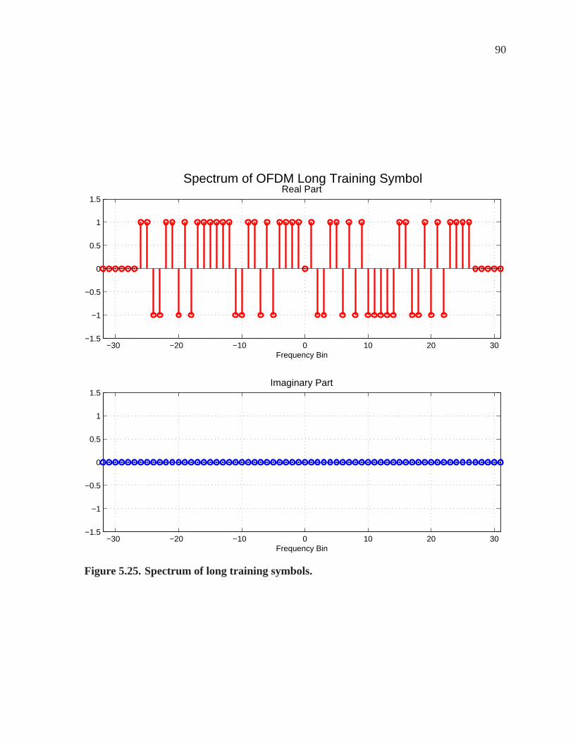
90
Spectrum of OFDM Long Training Symbol
−30 −20 −10 0 10 20 30−1.5
−1
−0.5
0
0.5
1
1.5
Frequency Bin
Imaginary Part
−30 −20 −10 0 10 20 30−1.5
−1
−0.5
0
0.5
1
1.5
Frequency Bin
Real Part
Figure 5.25. Spectrum of long training symbols.

91
− 1, 1,−1, 1, 1, 1, 1, 0, 1,−1,−1, 1, 1,−1, 1,−1, 1,−1,
− 1,−1,−1,−1, 1, 1,−1,−1, 1,−1, 1,−1, 1, 1, 1, 1]. (5.31)
The lack of copies in the OFDM frames is from the lack of zero packing in equation 5.31 and
so the symbols have lengthNfft and, along with the added cyclic prefix, the total length of the
long training symbols is2.5×Nfft. Again, we setNfft = 64 so that the long training symbol
is 64 samples long. With a sample time of1/20MHZ = 0.05µs the long training symbol
time is64× 0.05µs = 3.2µs. There are two long training symbols and a cyclic prefix of
length 32 so the total time for the long training symbols is2× 3.2µs+ 32× 0.05µs = 8µs.
Figure 5.26 shows the time series for the long training symbols with the cyclic prefix.
Figure 5.27 shows the time series of the complete preamble with 320 samples and
length16µs.
5.2.2 OFDM Frame Timing EstimationTiming estimation is broken into two parts, frame timing or packet detection and
symbol timing. In both cases we use the preamble for detection. Here we start with frame
timing and exploit the periodicity of the short training symbols using the auto-correlation as
described in [23]. From Appendix F, the cross-correlation function is defined as
f ⋆ g ≡∞∑
m=−∞f [−m]g[m]. (5.32)
The correlation of the signal with a delayed copy of itself isdefined as
A[n] =N∑
k=0
r(k + n)r[k + n+ L], (5.33)
whereA[n] is the output,r[n] is the received sequence,L is the length of one short symbol
and the length of the delay. There are several algorithms forcoarse timing but all use the
correlation properties of the short training symbols. In this analysis, the delay and correlate
algorithm presented in [23] and [9] is used. Figure 5.28 shows the block diagram for this
algorithm.
The top path,P (d), contains the cross-correlator and the bottom path,R(d), contains
the auto-correlator. Theδ value in the bottom path is to avoid division by zero. The
auto-correlator computes the power in the samples and is used to normalize the decision at the
threshold detector. The cross-correlator takes advantageof the periodicity in the short training

92
Time Series of Long Training Symbols
0 1 2 3 4 5 6 7 8Time [µ s]
Imaginary Part
0 1 2 3 4 5 6 7 8Time [µ s]
Real Part
Figure 5.26. Time series of long training symbols.

93
Preamble Sturcture for IEEE 802.11a
0 2 4 6 8 10 12 14 16Time [µ s]
Imaginary Part
0 2 4 6 8 10 12 14 16Time [µ s]
Real Part
Figure 5.27. Time series of preamble.
Figure 5.28. Delay and correlate algorithm.

94
symbols to locate the frame boundaries. These are defined mathematically as
P (d) =L−1∑
m=0
r(d+m)r(d+m+ L) (5.34)
R(d) =L−1∑
m=0
|r(d+m+ L)|2 , (5.35)
whereL is the length of the register in the moving average andr(d) is thedth sample of the
received signal.M(d) is the output of the correlator normalized by the received power and
then tested against a threshold level. Squaring helps mitigate the effects of large peak to
average power ratios common in OFDM. Figure 5.29 shows the output of the correlator, the
received power and the threshold detector for the received signal in Figure 5.30. The signal
starts after the first 50 samples and because a length of 16 wasused for the moving average
filter, the maximum value of the correlation and the power is not reached for 16 samples. Also
note that the timing estimateM(d) reaches a maximum at the 51st sample, which is the
correct timing.
One might wonder why the auto-correlation is used in determining the frame start
since the cross-correlation shows the symbol boundaries. The received signal will have a
carrier frequency offset as well as multipath interferenceand Gaussian noise. Figure 5.31
shows the effect of a200kHz frequency offset and7dB SNR on the time series input to the
delay and correlate algorithm.
Figure 5.32 shows the output of the cross-correlator, auto-correlator, and threshold
detector for a200kHz frequency offset and7dB SNR.
In both Figures 5.29 and 5.32, the falling edge of the packet detection can be
determined. Notice, however, that while in an ideal channel, Figure 5.29, the cross-correlation
function can also detect this edge simply by looking at the peak values while in a non-ideal
channel as in Figure 5.32, the peak values have changed and determining the frame timing
becomes difficult. For this reason the auto-correlation function is used to normalize the input
to the threshold detector. Even with poor channel conditions the frame is still detected,
although with a sample error. This sample error will need to be corrected with fine timing, or
symbol timing estimation.
5.2.3 Frequency Offset EstimationEstimation of frequency offset during the acquisition phase is performed in two parts.
Coarse frequency offset uses the short training symbols and fine frequency offset uses the
long training symbols. Both coarse and fine frequency estimation use the same algorithm,
correlation with the received signal and a delayed copy. Theconjugate product is then passed
to a phase detector that outputs the phase error.

95
Frame Timing Estimation With Ideal Channel
0 50 100 150 200 2500
0.5
1
1.5
Sample
Output of Coarse Timing Estimator
0 50 100 150 200 2500
5
10
15Bottom Path (Received Power)
Sample0 50 100 150 200 250
0
5
10
15Top Path (Correlation With Delyed Copy)
Sample
Figure 5.29. Output of the cross-correlator, the auto-correlator, and the thresholddetector.

96
IEEE 802.11a Preamble Prepended With 50 Samples
0 50 100 150 200 250 300 350 400−0.2
−0.15
−0.1
−0.05
0
0.05
0.1
0.15
0.2Imaginary Part
0 50 100 150 200 250 300 350 400−0.2
−0.15
−0.1
−0.05
0
0.05
0.1
0.15
0.2Real Part
Figure 5.30. Received signal with 50 samples prepended.

97
IEEE 802.11a Preamble Prepended With 50 Samples
0 50 100 150 200 250 300 350 400−0.2
−0.15
−0.1
−0.05
0
0.05
0.1
0.15
0.2Imaginary Part
0 50 100 150 200 250 300 350 400−0.2
−0.15
−0.1
−0.05
0
0.05
0.1
0.15
0.2Real Part
Figure 5.31. Time series of preamble with SNR≈ 7dB and frequency offset 200kHz.

98
Frame Timing Estimation With Frequency Offset=200kHz, SNR=7dB
0 50 100 150 200 2500
0.5
1
1.5
Sample
Output of Coarse Timing Estimator
0 50 100 150 200 2500
5
10
15Bottom Path (Received Power)
Sample0 50 100 150 200 250
0
5
10
15Top Path (Correlation With Delyed Copy)
Sample
Figure 5.32. Output of the cross-correlator, the auto-correlator, and the thresholddetector with SNR≈ 7dB and frequency offset 200kHz.

99
The maximum frequency offset allowed in the IEEE 802.11a standard (section
17.3.9.4) [12] is±20ppm for carrier frequencies between5.15− 5.825GHz. This means that
the maximum frequency offset between transmitter and receiver (for carrier frequency
5.825GHz) is
f∆ =(
40× 10−6) (
5.825× 10⁹)
(5.36)
= 233kHz. (5.37)
Hence any algorithm used to estimate and correct frequency offset needs to operate with this
amount of offset.
Suppose the received signal is
y(t) = x(t)ej2πf∆t, (5.38)
wherex(t) is the transmitted signal and∆f is the frequency offset. As stated previously, the
short training symbols have a length of 16 samples or0.8µs. Then the output of the conjugate
product from the correlation of the signal and the delayed copy is
y(t)y∗(t− δt) = |x(t)|2 ej2π∆f(δt). (5.39)
The frequency offset is found by taking the arctangent of both sides
∠y(t)y∗(t− δt) = ∠ |x(t)|2 ej2π∆fδt) (5.40)
∠y(t)y∗(t− δt) = 2π∆fδt (5.41)
∆f =∠y(t)y∗(t− δt)
2πδt(5.42)
whereδt is the symbol time. The output of the phase detector is based on the arctangent
function and thus has a range of[−π, π). This means that the maximum detectable frequency
offset using the conjugate product is
∆f =±π
2π(16)(
120GHz
) (5.43)
=±π
2π(0.8µs)(5.44)
= 625kHz, (5.45)
or about 107ppm at 5.825GHz, much greater than the allowablefrequency offset. By
comparison, using the long training symbols, the detectable frequency offset is
∆f =±π
2π(64)(
120GHz
) (5.46)
=±π
2π(3.2µs)(5.47)
= 156kHz (5.48)

100
or about 13ppm, much less than what is allowed. This is why theshort training symbols are
used for the coarse estimation and correction before using the long training symbols for fine
frequency estimation and correction. Figure 5.33 shows thefrequency estimation algorithm.
Figure 5.33. Frequency estimation algorithm.
Consider the example where the frequency offset is 200kHz. Figure 5.34 shows the
estimated phase of the received signal using the short training symbols where a 16 sample
delay is seen in the output. The poor phase estimation in the long training symbol portion is
because the algorithm uses a delay length of 16 where the longtraining symbols have a length
of 64. Figure 5.34 also shows the phase estimation using the long training symbols where a
delay of 64 samples occurs. The effects of frequency offset and correction on the time series
is shown in Figure 5.35
The previous example did not incorporate a phase locked loop(PLL) but instead the
phase estimation of the entire preamble was computed and theaverage of the phase error was
applied to the entire series. This is an impractical implementation because of the delay in
waiting for the entire preamble to arrive. We now consider anexample which uses a PLL with
the same 200kHz frequency offset. By trial and error the values θn = 2π/49 andζ =√2/2
were found makingki = 0.0594 andkp = 0.1638. The output of the phase detector and the
output of the loop filter are shown in Figure 5.36.
The accumulated phase of the variable controlled oscillator (VCO) and the VCO
output are shown in Figure 5.37. Notice that the frequency iscorrectly estimated but there is a
phase offset in the VCO output. This is referred to as residualfrequency offset and is dealt
with using the pilot symbols.
Lastly, the constellation of the received signal with and without frequency offset
compensation is seen in Figure 5.38. The phase offset seen inthe VCO output is also seen in
the corrected constellation.

101
Frequency Estimation and Correction
180 200 220 240 260 280 300 320−6
−4
−2
0
x 10−16 Phase Estimation After Fine Frequency Corretion With Long training Symbols
180 200 220 240 260 280 300 320−6
−4
−2
0
x 10−16 Phase Estimation of Long Training Symbols After Coarse Frequency Corretion
0 50 100 150 200 250 300 350−0.5
0
0.5Phase Estimation After Course Frequency Correction With Short Training Symbols
0 50 100 150 200 250 300 350−0.5
0
0.5Phase Estimation of Received Signal
Figure 5.34. Estimated phase.

102
Time Series of Received Signal With Frequency Correction
0 50 100 150 200 250 300 350−0.2
0
0.2Received Signal After Fine Frequency Correction
0 50 100 150 200 250 300 350−0.2
0
0.2Received Signal After Course Frequency Correction
0 50 100 150 200 250 300 350−0.2
0
0.2Recieved Signal With Frequency Offset of 200[KHz]
0 50 100 150 200 250 300 350−0.2
0
0.2Transmitted Signal
Figure 5.35. Time series with and without frequency offset correction.

103
Input and Output to Loop Filter
0 20 40 60 80 100 120 140 1600
0.01
0.02
0.03
0.04
0.05
0.06
0.07Loop Filter Output
0 20 40 60 80 100 120 140 1600
0.002
0.004
0.006
0.008
0.01Phase Error
Figure 5.36. Output of phase detector and loop filter.

104
0 100 200 300 400 500 600 700 800 900 10000
2
4
6
8
10
Rad
ians
Accumulated Phase VCO
0 100 200 300 400 500 600 700 800 900 1000
−1
0
1
2Real Part of Input and Output Phase
Input PhaseOutput Phase
0 100 200 300 400 500 600 700 800 900 1000
−1
0
1
2Imaginary Part of Input and Output Phase
Input PhaseOutput Phase
Figure 5.37. Accumulated phase and VCO output.

105
Figure 5.38. Constellation with and without frequency offset correction.
5.2.4 Symbol Timing EstimationSymbol timing or fine timing is performed after coarse timingand after frequency
offset correction. Fine timing estimation uses the cross-correlation of the known long training
symbol with the received long training symbol to determine the start and end of an OFDM
symbol and consequently the start and end of the FFT window. As discussed in section 5.2.2,
the cross correlation is sensitive to frequency offset and this explains the importance of
correcting frequency offset before performing symbol timing estimation [16].
During the frame timing estimation, the starting edge of thepacket was determined but
within the packet symbol timing errors can be present. The cross-correlation of the known
long training symbol and the received long training symbol can be determined by
r(n) =M∑
m=0
r′LTS(m)rLTS(m− n), (5.49)
wherer′LTS is the received long training symbols,rLTS is the known long training symbol,
andM is the length of the long training symbol. In Appendix F, it isshown that there is a
relationship between the cross-correlation operator and the convolution operator. It is
desirable to use the convolution operation since it can be performed using the FFT, which
reduces the number of computations [19]. Hence, we have the symbol timing estimation as
r(n) = r′LTS(n) ∗ rLTS(−n), (5.50)
where∗ is the convolution operator.

106
There are two and a half long training symbols (the half symbol provided by the cyclic
prefix) in the IEEE802.11a standard. Thus the cross-correlation should have three peaks, the
first being about half the magnitude of the other two, which can be seen in Figure 5.39.
Fine Timing Estimation
16 32 48 64 80 96 112 128 144 160 192 256 320
0
0.5
1
Cross−Correlation of Known LTS and Received LTS
16 32 48 64 80 96 112 128 144 160 192 256 320Sample
IEEE 802.11a Preamble
Figure 5.39. Cross-correlation of long training symbol.
The first peak corresponds to the end of the cyclic prefix and the other two peaks
correspond to the ends of the two long training symbols whichhave the same length as the
OFDM symbol.

107
5.2.5 Channel EstimationIn Chapter 2, the effects of a multipath channel, namely frequency selectivity, were
discussed. Thus far only frequency and timing offsets have been estimated and corrected. The
effect of a multipath channel on the received constellationdiagram is seen in Figure 5.40.
−1.5 −1 −0.5 0 0.5 1 1.5−1.5
−1
−0.5
0
0.5
1
1.5Received Signal With Channel Distortion
In−Phase
Qua
drat
ure
Figure 5.40. Effects of multipath channel on received constellation.
To counter these effects, an equalizer is used. In a conventional single carrier system
equalization takes place in the time domain where the equalizer can be computationally
intensive.
In an OFDM system, the equalization takes place in the frequency domain with the
advantage that if the sub-channels are sufficiently narrow bands, the frequency fading of the
channel can be considered flat within each sub-channel [9].

108
Let Y be the received signal,X the transmitted signal, andH the channel frequency
response. Then
Y [k] = H[k]X[k] + Z[k], (5.51)
whereZ is the noise. Here we take advantage of the property of Fourier transforms, that
convolution in the time domain corresponds to the product inthe frequency domain. As stated
in Chapter 2, it is assumed that the channel is stationary during each transmitted packet. We
have then, settingZ[k] = 0,
H[k] =Y [k]
X[k]. (5.52)
In this way, the channel can be estimated but only if the transmitted signal is known. To this
end, the long training symbols are used. Recall that the long training symbols use all
sub-carriers (except DC) so that all used sub-carrier equalizer gains are found. Equation 5.52
describes the channel frequency response for each sub-carrier but the inverse is needed to
counter its effects:
|H[k]|2 = H[k]H[k] (5.53)
H−1[k] =H[k]
|H[k]|2 . (5.54)
It is common to average the equalizer gains over the two long training symbols to help
mitigate the effects of the noise. Figure 5.41 shows the channel frequency response and the
channel estimation using the above method. Notice that the noise in the channel affects the
estimation. Figure 5.42 shows the received constellation after the channel estimation has been
applied to Figure 5.40.
5.2.6 Residual Frequency OffsetIn Section 5.1.1, carrier frequency offset was simulated and in Section 5.2.3, a method
of estimation and correction was put forward. The simulation showed very precise estimation
that left the system with negligible errors. In real implementations of frequency offset
estimation, the frequency offset is not constant (as simulated in section 5.1.1) and the system
itself introduces thermal noise and phase degredation, which increases the error in carrier
frequency offset [5]. This error is a residual frequency offset and while it may be small the
accumulation of the offset can destroy the orthogonality ofthe sub-carriers.
To continue tracking the frequency offset, each OFDM symbolcontains four pilot
subcarriers at frequency bins -21, –7, 7, 21 and are BPSK modulated using a pseudo-binary
sequence [12]. The psuedo-binary sequence prevents spectral lines and can be generated by
the data scrambler in Figure 5.43 [12].

109
−30 −20 −10 0 10 20 30−60
−50
−40
−30
−20
−10
0
Frequency bin
|H[f]
|2 [dB
]
Multipath Channel with SNR=43.3486
Channel EstimationChannel Frequency Response
Figure 5.41. Channel estimation.

110
−1.5 −1 −0.5 0 0.5 1 1.5−1.5
−1
−0.5
0
0.5
1
1.5Received Signal With Channel Correction
In−Phase
Qua
drat
ure
Figure 5.42. Received constellation after channel correction.
Figure 5.43. Scrambler used to generate psuedo-binary pilot sequence.

111
The scrambler is initiated with all ones and produces the cyclically extended 127
element sequenceP0 in equation 5.55:
P0..126v = {1, 1, 1, 1,−1,−1,−1, 1,−1,−1,−1,−1, 1, 1,−1, 1,−1,−1, 1, 1,−1, 1, 1,
− 1, 1, 1, 1, 1, 1, 1,−1, 1, 1, 1,−1, 1, 1,−1,−1, 1, 1, 1,−1, 1,−1,−1,−1, 1,
− 1, 1,−1,−1, 1,−1,−1, 1, 1, 1, 1, 1,−1,−1, 1, 1,−1,−1, 1,−1, 1,−1, 1, 1,
− 1,−1,−1, 1, 1,−1,−1,−1,−1, 1,−1,−1, 1,−1, 1, 1, 1, 1,−1, 1,−1, 1,
− 1, 1,−1,−1,−1,−1,−1, 1,−1, 1, 1,−1, 1,−1, 1, 1, 1,−1,−1, 1,−1,−1,
−1, 1, 1, 1, 1, 1,−1,−1,−1,−1,−1,−1,−1} (5.55)
The algorithm for tracking frequency is similar to that of course frequency estimation.
After baseband demodulation, the pilots are extracted and the phases of the pilots are
compared to the phases of the previous pilots. The phase offset is sent to a loop filter, then to a
VCO, and multiplied to the input of the FFT. Appendix G furtherdiscusses the phase lock
loop and Appendix H contains MATLAB code to simulate the PLL.Figure 5.44 shows one
possible residual phase tracking configuration.
Figure 5.44. Residual frequency tracking.

112
CHAPTER 6
MULTIPLE INPUT MULTIPLE OUTPUT
One of the first uses of multiple antennas was in 1901 when Guglielmo Marconi used
multiple transmit antennas to transmit the Morse symbol ”S”(three short dots) from Poldhu,
Cornwall, England, to Signal Hill in St. John’s Newfoundland, a distance of 2,200 miles. The
multiple antennas transmitted the same signal in a scheme called spacial diversity. In the
1940’s, submarines began experimenting with active sonar.Multiple sound transmitters were
used with delays added, allowing certain areas to be covered. This is called beamforming and
is a type of space-time diversity.
Though multiple antennas have been used for some time, standards such as
IEE802.11n (Wi-Fi) and IEEE802.16 (WiMAX) have brought thetechnology to consumer
products. The technology has made possible the increased throughput required for many
applications and takes advantage of the ubiquitous wireless multipath channel. Multiple input
multiple output (MIMO)1 not only increases quality of service but can achieve data rates near
channel capacity, and thus using the bandwidth more efficiently. The increase in quality of
service means an increase in the coverage area via increasedSNR.
In this chapter, we will explore MIMO using the IEEE802.11n standard for illustrating
the implementation in a realizable system. The three areas of interest that will be discussed
include space-time coding (STC), spatial division multiplexing (SDM), and transmit
beamforming.
6.1 SPACE T IME CODING
Space time coding (STC) algorithms are used to increase the reliability of the
reception of data by transmitting multiple copies of the data stream. This redundancy aids in
combating the fading present in wireless channels. This is because there is an increase in
probability that if one transmission experiences poor channel conditions which result in
errors, that the other transmission(s) are recoverable. Itis reasonable to assume that channel
conditions for each path are not the same for each spatial stream[21].
Space time codes be categorized as either space time trelliscodes (STTC) or space
time block codes (STBC). STTCs use redundancy to achieve codingand diversity gains2
operating on one input symbol at a time and outputting a vector whose length is the number of
1The input output in MIMO does not refer to the transceiver butto the number of spatial streams input andoutput to the channel
2The increase in the SNR is due to the diversity scheme, in thiscase the number of transmit antennas

113
transmit antennas. STBCs, by contrast, operate on blocks of input symbols and output a
matrix where the number of rows is the number of transmit antennas and the columns
represent time. STBCs also offer full diversity but with much less encoder decoder
complexity [22].
6.1.1 Space Time Trellis CodesThe IEEE802.11 standard allows for the use of the STTC convolutional codes as a
means of forward error correcting codes[12]. Though the IEEE802.11n standard also allows
for low density parity check codes (LDPC) and turbo codes, we will focus on the widely used
convolutional codes as presented in IEEE802.11a.
Convolutional codes are characterized by the following three parameters: the number
of output bits,n, the number of input bits,k, and the constraint length,L. The rate of the code
is the ratio of input bits to output bits,k/n. Convolutional codes also have associated
generating polynomials, the number of which depends on the number of output bits, usually
written in octal notation. The convolutional code shown in Figure 6.1 is a (2,1,7) code with
rate1/2 and generating polynomialsg0 = 1338 andg1 = 1718, which is the industry standard
[15]. The generating polynomials, in the more insightful binary notion, areg0 = 10110112
andg1 = 11110012 and describe the XORing of the current and shifted values in the registers.
Figure 6.1. Rate1/2 convolutional encoder with constraint length 7.
The convolutional coder is a finite state machine with assumed initial null state and as
such, has two diagrams to show the state transitions. The four state convolutional encoder

114
shown in Figure 6.2 is described by the state diagram shown inFigure 6.3 and the trellis
diagram as seen in Figure 6.4. Unlike the state diagram, the trellis diagram adds a time
component showing the output and states for a given input; a red line represents an input of
one and a black line an input of zero. Each path of the trellis diagram corresponds to an
encoded sequence.
Figure 6.2. Four state convolutional encoder.
Figure 6.3. State diagram for encoderin Figure 6.2.
Figure 6.4. Trellis diagram for convolutional encoder in Figure 6.2.
Both the state and trellis diagrams show two branches to and from each state and it can
be shown that for a convolutional encoder withm memory elements there are2m branches at
each of the2m states. Also note that not all state transitions are possible, hence only certain
paths can exist. It is this feature that will be exploited to decode the received bit stream.

115
6.1.2 Space Time Block CodesSpace time block codes differ from STTCs in that they operate on a block of data
instead of one piece of data during each time interval. In 1998 Siavash Alamouti proposed a
two antenna STBC that does not require any bandwidth expansion or channel state
information (CSI) at the transmitter [1]. His two antenna scheme was generalized to
incorporate more antennas and thus increasing the block size operated on, however, the two
antenna transmit scheme is a rate 1 code and it has been shown that this is the only
configuration to achieve this rate. Here we look at the case presented in [1] for two transmit
antennas.
The Alamouti coded OFDM system is shown in Figures 6.5 and 6.6. As before, we
consider the Rayleigh multipath fading channel and a delay spread less than the cyclic prefix
length. It is important to remember that using OFDM as a modulation scheme allows the
assumption of a flat fading channel for each sub-carrier.
Figure 6.5. Alamouti for two transmit antennas.
Figure 6.6. Alamouti for one receive antenna.
The Alamouti scheme takes advantage of the spacial dimension by transmittings1from antenna 1 ands2 from antenna 2 wheresi are the OFDM symbols to be transmitted.
Then,−s∗2 ands∗1 are sent from antennas 1 and 2 respectively, as seen in Table 6.1.

116
Table 6.1. Alamouti TransmissionScheme
Antenna 1 Antenna 2
Time t s1 s2Time t+T −s∗2 s∗1
Since two symbols are transmitted during two time periods, the coding scheme has
rate 1. Thus, for the antenna scheme in Figure 6.7, the received signals are
y1 = H1s1 +H2s2 + η1 (6.1)
y2 = −H1s∗2 +H2s
∗1η2, (6.2)
whereyk is the received signal for thekth antenna,Hk is the multipath channel from thekth
transmit antenna, andηi is the additive noise for theith symbol period.
Figure 6.7. Channel for two transmitantennas and one receive antenna.
At the receiver, the received signal is demodulated with theFFT after the removal of
the cyclic prefix and each subchannel undergoes decoding. The two received symbols for the
nth subchannel are
y1 = a1x1 + a2x2 + η1 (6.3)
y2 = −a1x∗2 + a2x∗1 + η2, (6.4)
whereyl is the received symbol on thenth subcarrier from thelth OFDM symbol,xm is the
mth symbol,ak is the flat fading channel gain for thenth subcarrier from antennak, andη is

117
as before. Rewriting as vectors we have
y1 =[
a1 a2
]
[
x1
x2
]
+ η1 (6.5)
y2 =[
a1 a2
]
[
−x∗2x∗1
]
+ η2 (6.6)
(6.7)
and combining both received symbols into one equation, we have[
y1
y∗2
]
=
[
a1 a2
a∗2 −a∗1
][
x1
x2
]
+
[
η1
η∗2
]
. (6.8)
For convenience let
A =
[
a1 a2
a∗2 −a∗1
]
. (6.9)
Then to solve for the symbolsx1 andx2 we need the inverse ofA. ForA to have an inverse it
needs to be square and have determinant zero. To avoid such a case, we will use the
Moore-Penrose psuedoinverse,A+ = (AHA)−1AH . Solving forA+, we have
AHA =
[
a∗1 a2
a∗2 −a1
][
a1 a2
a∗2 −a∗1
]
(6.10)
=
[
|h1|2 + |h2|2 0
0 |h1|2 + |h2|2
]
(6.11)
(
AHA)−1
=
[
1|h1|2+|h2|2
0
0 1|h1|2+|h2|2
]
. (6.12)
Thus, we have[
x1
x2
]
=(
AHA)−1
AH
[
y1
y∗2
]
(6.13)
=
[
1|h1|2+|h2|2
0
0 1|h1|2+|h2|2
]
AH
(
A
[
x1
x2
]
+
[
η1
η∗2
])
(6.14)
=
[
x1
x2
]
+(
AHA)−1
AH
[
η1
η∗2
]
. (6.15)
For the case of two receive antennas, as seen in Figure 6.8, the received symbols for
thenth subcarrier on antenna 1 are[
y11
y12
]
=
[
a11 a12
a21 a22
][
x1
x2
]
+
[
n11
n12
]
(6.16)

118
Figure 6.8. Channel for two transmitantennas and two receive antennas.
and the received symbols on antenna 2 are[
y11
y12
]
=
[
a11 a12
a21 a22
][
x1
x2
]
+
[
n11
n12
]
. (6.17)
Combining the two into one equation yields,
y11
y12
y∗21
y∗22
=
a11 a12
a21 a22
a∗12 −a∗11a∗22 −a∗21
[
x1
x2
]
+
n11
n12
n∗21
n∗22
. (6.18)
For convenience, we define
A =
a11 a12
a21 a22
a∗12 −a∗11a∗22 −a∗21
. (6.19)
As before, we define the Moore-Penrose pseudoinverse asA+ = (AHA)−1AH and solving for
(AHA)−1 we have
AHA =
[
a∗11 a∗21 a12 a22
a∗12 a∗22 −a22 −a21
]
a11 a12
a21 a22
a∗12 −a∗11a∗22 −a∗21
(6.20)
=
[
|a11|2 + |a21|2 + |a12|2 + |a22|2 0
0 |a11|2 + |a21|2 + |a12|2 + |a22|2
]
(6.21)

119
(
AHA)−1
=
[
1|a11|2+|a21|2+|a12|2+|a22|2
0
0 1|a11|2+|a21|2+|a12|2+|a22|2
]
. (6.22)
Solving for the received symbols we have
[
x1
x2
]
=(
AHA)−1
AH
y11
y12
y∗21
y∗22
(6.23)
=(
AHA)−1
AH
n11
n12
n∗21
n∗22
(6.24)
=
[
x1
x2
]
+(
AHA)−1
AH
n11
n12
n∗21
n∗22
. (6.25)
Both schemes show the need for an accurate channel estimationto find the channel
inverse. This is discussed in section 6.5.
6.2 VITERBI DECODER
The Viterbi algorithm was developed in 1967 by Andrew Viterbi, which is essentially
a maximum likelihood decoder [18]. The Viterbi decoder’s complexity is not dependent on
the number of symbols in a codeword sequence and takes advantage of the structure of the
trellis diagram, to further reduce the computations. Two implementations of the Viterbi
decoder used are the hard decision decoder and the soft decision decoder.
6.2.1 Hard Decision Viterbi DecoderIn the convolutional encoder in Figure 6.2, there are two outputs for each input.
Hence, to decode, we take two bits at a time and compute the hamming distance, the branch
metric, the path metric, and the surviving path. The Hammingdistance is the number of bits in
error between the received and transmitted sequence. The branch metric is the sum of the path
metric and the Hamming distance and the path metric is the minimum of the branch metrics
for each state. The hard decision decoder has input of one bitprecision binary symbols.
As an example, suppose the received bit sequence from the four state encoder in
Figure 6.2 is01, 01, 10, 01, 00 with the assumption that the encoder has initial state00 and is
known at the receiver. Figure 6.9 shows the trellis diagram with the ordered pair (Hamming
distance, branch metric) and the path metric labeled at eachstate.

120
Figure 6.9. Viterbi decoding algorithm.
In Figure 6.9, the most likely path is the path whose metric islowest, which is in red.
At each time interval the Hamming distance is computed as thenumber of bits in error from
the received bits and the output of the encoder between states. Note that fort ≥ 3, each state
has two previous states in common. This is where the branch metrics are compared and the
lowest is chosen. In the event that both branch metrics are the same, as is the case for state
(11) at t = 4 in Figure 6.9, the path can be chosen randomly or by a constantdecision such as
the top or bottom path. The(10) state att = 5 has the lowest accumulated error so starting
from this state the decoder traces back following the lowestbranch metric. The progression of
states fromt = 0 to t = 5 is 00, 10, 11, 11, 01, 10. Table 6.2 shows the state transitions and the
input to the convolutional encoder.
Table 6.2. Encoder Transitionand Inputs
State Transition Encoder Input
00→ 10 110→ 11 111→ 11 111→ 01 001→ 10 1
Thus, the most likely input sequence was1, 1, 1, 0, 1 with one received error. In this
example the trellis diagram for the entire sequence was computed but in practice this is not
practical for long sequences as this will increase the amount of delay. The length of the trellis
used is called the traceback depth and it is clear from the example att = 1 that too short of a
traceback depth causes errors in the decoding. The general rule is a traceback depth of five

121
times the constraint length and depths greater than this do not see much improvement in
performance. The exact traceback or decision depth is foundby simulation in practice
although analytic traceback techniques exist based on the free distance. If puncturing is
applied, the traceback depth is increased to 7 to 9 times the constraint length.
6.2.2 Soft Decision Viterbi DecodingThe soft decision Viterbi decoder is similar to the hard decision decoder but instead of
using one bit precision, multiple bits are used to convey thereliability of the values. Table 6.3
shows one such scheme for three bit precision. Figure 6.10 shows the relationship between
the input and output for the three bit quantized soft decision decoder.
Table 6.3. Soft Decision ViterbiDecoder
Quantized level Reliability
000 Strongest 0001 Relatively Strong 0010 Relatively Weak 0011 Weak 0100 Weak 1101 Relatively Weak 1110 Relatively Strong 1111 Strongest 1
The decision valueD is computed as
D =1
2
√
1
2EsN0
(6.26)
whereEsN0
is the symbol signal to noise ratio. The width of the decisionregions is√N02
k
wherek is the bit precision andN0 is the noise PSD. The branch and path metrics are
computed with the three bit values and the add, compare, and select (ACS) algorithm of the
hard decision decoder is applied. Figure 6.11 shows a comparison of the hard and soft
decision decoders.
6.3 SPATIAL DIVISION M ULTIPLEXING
Spatial division multiplexing (SDM) is a technique used to transmit independent data
streams from each antenna at the same time and carrier frequency. To separate the signals
which interfere with each other, the number of receive antennas must be greater than or equal
to the number of transmit antennas and knowledge of the channel is needed at the receiver.
The decoding is, in general, less complex than STCs.

122
−3D −2D −1D 1D 2D 3D000−−>0
001−−>1
010−−>2
011−−>3
100−−>4
101−−>5
110−−>6
111−−>7Three bit quantizer input/output relationship
Input decision level
Out
put
Figure 6.10. Input/output relationship for 3 bit quantizer.

123
0 1 2 3 4 5 6 7 8 9 1010
−5
10−4
10−3
10−2
10−1
Eb/No [dB]
Bit
Err
or R
ate
BER for Binary Convolutional Code with Viterbi decoding for BPSK in AWGN
Theoretical − UncodedSimulation − Hard ViterbiSimulation − Soft Viterbi
Figure 6.11. Comparison of hard and soft Viterbi decoding.

124
We consider two types of spatial multiplexing developed at Bell labs. Diagonal Bell
labs layer space time (D-BLAST) transmits successive encoded data symbols on different
antennas in a cyclic fashion. Vertical Bell labs layered space time (V-BLAST) is much less
computationally intensive than D-BLAST with the detection at the receiver performed
vertically at each time interval. Figure 6.12 shows the encoder and the output for both
D-BLAST and V-BLAST [6].
Figure 6.12. D-BLAST and V-BLAST layered transmission scheme.
As seen in Figure 6.12, both the D-BLAST and the V-BLAST encoders demultiplex
the incoming bit stream into parallel substreams using a serial to parallel conversion where
each substream is then encoded separately. For V-BLAST, the substreams are then transmitted
on separate antennas, but for D-BLAST, the substreams are distributed across the different
antennas in layers.
The decoding process for D-BLAST is more computationally intensive than that of
V-BLAST and increases in computational load with increasingnumber of transmit
antennas[6]. Notice that att = 0 only one antenna is transmitting so receiving the symbol is
straight forward. Att = 1 the next symbol in the layer (substream) has interference from a
second antenna. Receiving the second symbol in the layer requires the use of minimum mean
square error (MMSE) or zero forcing nulling (ZF-nulling) toignore the symbol interference
from the next layer [6]. The process continues until the layer has been received and then is
decoded. This decoded layer is then subtracted from the nextlayer and the process continues.
It is vital that the decoding of the layer is error free as it affects the decoding of the successive
layers. Because the layer cannot be decoded until all the symbols in the layer are received a
delay is introduced and there is a loss in capacity at the startup.
The decoding process for V-BLAST is less computationally intensive and involves
three basic steps: filtering, slicing, and cancellation. Ifchannel coding is used in conjunction

125
with V-BLAST, then the demodulated symbols must be buffered until the block can be
decoded. Several other types of decoders that can be used such as the maximum likelihood
(ML) decoder, zero forcing (ZF), and minimum mean square error (MMSE). An iterative
method can also be applied by ordereing the spatial streams by SNR. The stream with the
highest SNR is decoded first, treating the others as noise andthen is canceled so the next
highest SNR stream can be decoded [29].
6.4 BEAMFORMING
Some of the earliest examples of beamforming were seen in sonar where multiple
transmit arrays would employ delays to direct the coverage area to the intended target. By
directing the coverage area in wireless devices, the numberof users can be increased as
coverage can be extended or shaped to include only certain users as needed and the
interference from multiple users can be reduced as seen in Figure 6.13. Beamforming is an
option in the IEEE802.11n standard [15] and other communication standards like IEEE802.16
(WiMAX). Future amendments to IEEE802.11 will include beamforming as a means to
achieving data rates in the multi Gbps [20].
There are several ways to achieve beamforming but here we consider a technique
where each transmit antenna transmits the same signal at thesame frequency but with a phase
shift. As an example, suppose we have the three transmit antennas in the configuration seen in
Figure 6.14.
We want to find the contribution from each antenna to the pointA in Figure 6.14:
S(θ, r) = s0(r) + s1
(
√
x21 + y21 + φ1
)
+ s2
(
√
x22 + y22 + φ2
)
(6.27)
= s0(r) + s1
(√
(d− r cos θ)2(r sin θ)2 + φ1
)
+ s2
(√
(r cos θ − 2d)2(r sin θ)2 + φ1
)
(6.28)
=
(N−1)/2∑
n=(N−1)/2
sn
(
√
(r cos θ − nd)2 + (r sin θ)2 + φn
)
. (6.29)
In equation 6.29,S(θ, r) is the signal strength at the point(θ, r) from the center antenna,sn()
is the signal strength from thenth antenna,N is the number of antennas (here it must be odd),
andφn is the time delay for thenth antenna. Figure 6.15 demonstrates the signal strength for
three and five antenna configurations. For convenienceφn = nφ1, that is, the delays are
integer multiples ofφ1.
6.5 CHANNEL ESTIMATION
As seen in previous sections, accurate estimation of the channel is useful and in some
cases necessary. In Section 5.2.5 we discussed a method of using the long training symbols to

126
Figure 6.13. Directing coverage area tointended users using beamforming.
Figure 6.14. Three isotropic antenna configuration.

127
0.2
0.4
0.6
0.8
1
30
210
60
240
90
270
120
300
150
330
180 0
3 Antennas, Distance = 10, Relative phase delay = 10
0.2
0.4
0.6
0.8
1
30
210
60
240
90
270
120
300
150
330
180 0
3 Antennas, Distance = 10, Relative phase delay = 40
0.2
0.4
0.6
0.8
1
30
210
60
240
90
270
120
300
150
330
180 0
5 Antennas, Distance = 5, Relative phase delay = 25
0.2
0.4
0.6
0.8
1
30
210
60
240
90
270
120
300
150
330
180 0
5 Antennas, Distance = 5, Relative phase delay = 40
Figure 6.15. Signal strength for (a) three antennas, distance 10, and relative phase delay10, (b) three antennas, distance 10, and relative phase delay 40, (c) five antennas,distance 2, and relative phase delay 25, and (d) five antennas, distance 5, and relativephase delay 40.

128
estimate the channel, but this was for the single-input single-output case. Here we consider a
scheme also using training symbols for the multiple input multiple output case as seen in
Figure 6.16.
Figure 6.16. MIMO channel.
As before, the received signal is
Y [k] = H[k]X[k] + Z[k] (6.30)
whereX is the frequency domain symbol,H is the channel frequency response andZ is the
frequency response of the noise. The channel estimate is then
H[k] =Y [k]
X[k](6.31)
and the inverse of the channel estimate is then∣
∣
∣H[k]
∣
∣
∣
2
= H[k]H∗[k] (6.32)
H−1[k] =H∗[k]∣
∣
∣H∗[k]
∣
∣
∣
2 . (6.33)
As before, to find the estimate of the channel, the transmitted symbol must be known at the
receiver. Again, we use the long training symbols but there are two techniques to implement
them. The first is to transmit one training symbol on each transmitter as seen in Figure 6.17.
The procedure for extracting the channel estimates is then reduced to two SISO channel
estimates.

129
Figure 6.17. Alternate transmission of long preamble.
The second is to transmit the even frequency bins from antenna one and the odd
frequency bins from antenna two. Then in the next symbol period transmit the odd frequency
bins from antenna one and the even frequency bins from the antenna two, as seen in
Figure 6.18. To extract the channel estimates, the same procedure is employed as with the
SISO channel, with the exception that even and odd frequencybins need to be taken into
account.
Figure 6.18. Alternating even and odd frequencies.

130
CHAPTER 7
CONCLUSION
This thesis presented an introduction to MIMO-OFDM, specifically, the topics of the
channel, OFDM, synchronization, and MIMO. Mathematical descriptions of the channel,
OFDM, and synchronization, were given as well as MATLAB simulations to verify, illustrate
concepts, or present a practical implementation. Chapter two detailed the effects present in a
wireless multipath channel and the importance of the channel model. To that end, a frequency
domain channel model was given and simulated for the wireless multipath fading channel.
Chapter three briefly reviewed some of the modulation schemesused in digital
communications and used throughout this thesis. Chapter four gave a comparison of single
carrier systems and multicarrier systems as the motivationfor OFDM. Mathematical
definitions were presented on modulation and demodulation in the presence of a channel. This
gave a basis for understanding the synchronization errors common to OFDM.
In Chapter five, a detailed discussion of synchronization errors was presented.
Mathematical descriptions of the errors and simulations ofthe errors were presented to
illustrate the effect that timing and frequency offsets have on the uncoded constellations. The
second half of Chapter five showed how the synchronization errors could be estimated at the
receiver and corrected. For each type of synchronization error, algorithms were presented and
implemented in a MATLAB simulation. As an extension to OFDM,Chapter six presented
MIMO as a way to increase performance in a communication system. Three topics were
showcased along with examples of each. Space time coding techniques such as convolutional
codes and the Alamouti algorithm were shown to increase the reliability by transmitting
multiple copies. Both had coding gains but the Alamouti scheme also introduced spatial gain.
A maximum likelihood detector, the Viterbi decoder, was also presented as a way to decode
the convolutional encoder. Two types of spatial multiplexing, D-BLAST and V-BLAST, were
shown to be an effective way to increase the overall data rateby transmitting multiple
independent streams. Lastly, beamforming was introduced as a way to direct the coverage
area. In this way, more users can be serviced by the reductionof interference from multiple
users. It is hoped that after reading this thesis the reader has a better understanding of channel
models, MIMO-OFDM, the effects of the channel on OFDM, and the ways in which errors
are estimated and corrected.
This thesis aimed to be an introductory look into OFDM. Future systems will include
MIMO-OFDM and, as such, there is a lot of research being done in this area. One of the

131
assumptions made about the channel was that it was static. While this assumption works well
for standards such as IEEE802.11, it does not work well for cell phones and other wireless
devices. In the future, we may see many devices that must be able to operate at speeds were
Doppler shifts affect data transmission.
Another consideration is the techniques used in space time coding. Turbo codes and
low density parity-check codes are now replacing convolutional codes. Also, only the 2x2
MIMO case was considered for STBCs.

132
BIBLIOGRAPHY
[1] S. ALAMOUTI , A simple transmit diversity technique for wireless communications,IEEE Journal on Selected Areas in Communications, 16 (1998),pp. 1451 –1458.
[2] A. A NTONIOU, Digital Signal Processing, McGraw-Hill, New York, New York, 2006.
[3] R. CHANG, Synthesis of band-limited orthogonal signals for multi-channel datatransmission, Bell System Technical Journal, 46 (1966), pp. 1775–1796.
[4] CISCO. Cisco visual networking index: global mobile data traffic forecast update.n.d.http://www.cisco.com/en/US/solutions/collateral/ns341/ns525/ns537/ns705/ns827/white paperc11-520862.html, accessed November 2011.
[5] N. EGASHIRA, H. TAKAYAMA , AND T. SABA , Improvement of cci compensationaccuracy using feedback phase tracking in mimo-ofdm systems, in GlobalTelecommunications Conference 2004., vol. 2, Dallas, Texas, 2004, IEEE.
[6] G. J. FOSCHINI, Layered space-time architecture for wireless communication in afading environment when using multi-element antennas, Bell Laboratories TechnicalJournal, 1 (1996), pp. 41–59.
[7] R. G. GALLAGER, Principles of Digital Communications, Cambridge University Press,Cambridge, UK, 2008.
[8] F. HARRIS, Lets assume the system is synchronized, in Globalization of Mobile andWireless Communications, R. Prasad, S. Dixit, R. van Nee, and T.Ojanpera, eds.,Signals and Communication Technology, Springer, Netherlands, 2011, pp. 311–325.
[9] F. J. HARRIS, Orthogonal frequency division multiplexing. Unpublished notes, 2010.
[10] H. HASHEMI, The indoor radio propagation channel, Proceedings of the IEEE, 81(7)(1993), pp. 943 –968.
[11] V. HAYES ET AL., Ieee standard for information technology- telecommunications andinformation exchange between systems-local and metropolitan area networks-specificrequirements-part 11: Wireless lan medium access control (mac) and physical layer(phy) specifications, IEEE Std 802.11-1997, (1997), pp. i –445.
[12] , Supplement to ieee standard for information technology - telecommunications andinformation exchange between systems - local and metropolitan area networks - specificrequirements. part 11: Wireless lan medium access control (mac) and physical layer(phy) specifications: High-speed physical layer in the 5 ghzband, IEEE Std802.11a-1999, (1999), pp. i –82.
[13] G. JANSSEN, P. STIGTER, AND R. PRASAD, Wideband indoor channel measurementsand ber analysis of frequency selective multipath channelsat 2.4, 4.75, and 11.5 ghz,IEEE Transactions on Communications, 44 (1996), pp. 1272 –1288.
[14] S. J. KERRY ET AL., Ieee standard for information technology- telecommunications and

133
information exchange between systems- local and metropolitan area networks- specificrequirements part ii: Wireless lan medium access control (mac) and physical layer (phy)specifications, IEEE Std 802.11g-2003 (Amendment to IEEE Std 802.11, 1999 Edn.(Reaff 2003) as amended by IEEE Stds 802.11a-1999, 802.11b-1999, 802.11b-1999/Cor1-2001, and 802.11d-2001), (2003), pp. i –67.
[15] , Ieee standard for information technology–telecommunications and informationexchange between systems–local and metropolitan area networks–specific requirementspart 11: Wireless lan medium access control (mac) and physical layer (phy)specifications amendment 5: Enhancements for higher throughput, IEEE Std802.11n-2009 (Amendment to IEEE Std 802.11-2007 as amendedby IEEE Std802.11k-2008, IEEE Std 802.11r-2008, IEEE Std 802.11y-2008, and IEEE Std802.11w-2009), (2009), pp. c1 –502.
[16] R. V. NEE AND R. PRASAD, OFDM for Wireless Multimedia Communications, ArtechHouse Publishers, Boston, Massachusettes, 2000.
[17] H. NIKOOKAR AND H. HASHEMI, Phase modeling of indoor radio propagationchannels, IEEE Transactions on Vehicular Technology, 49 (2000), pp.594 –606.
[18] J. OMURA, On the viterbi decoding algorithm, IEEE Transactions on InformationTheory, 15 (1969), pp. 177 – 179.
[19] P. V. O’NEIL, Advanced Engineering Mathematics, PWS-Kent Publishing Company,Boston, Massachusetts, 4 ed., 1995.
[20] E. PERAHIA , C. CORDEIRO, M. PARK , AND L. YANG, Ieee 802.11ad: Defining thenext generation multi-gbps wi-fi, in Consumer Communications and NetworkingConference, Las Vegas, NV, jan. 2010, IEEE, pp. 1 –5.
[21] R. PRASAD, OFDM Wireless Communications Systems, Artech House Publishers,Boston, Massachusetts, 2004.
[22] S. SANDHU , R. HEATH, AND A. PAULRAJ, Space-time block codes versus space-timetrellis codes, in IEEE International Conference on Communications, vol. 4,Helsink,Finland, 2001, IEEE, pp. 1132 –1136.
[23] T. SCHMIDL AND D. COX, Low-overhead, low-complexity [burst] synchronization forofdm, in IEEE International Conference on Communications., Dallas, Tx, 1996, IEEE.
[24] B. SKLAR , Digital Communications: Fundamentals and Applications, Prentice Hall,Upper Saddle River, New Jersey, 2nd ed., 2001.
[25] M. SPETH, S. FECHTEL, G. FOCK, AND H. MEYR, Optimum receiver design forwireless broad-band systems using ofdm. i, IEEE Transactions on Communications, 47(1999), pp. 1668 –1677.
[26] D. TSE AND P. VISWANATH, Fundamentals of Wireless Communication, CambridgeUniversity Press, Cambridge, UK, 2005.
[27] L. V ERMA AND S. LEE, Proliferation of wi-fi: Opportunities in ce ecosystem, inConsumer Communications and Networking Conference, Las Vegas, NV, 2011, IEEE,

134
pp. 213 –217.
[28] S. WEINSTEIN AND P. EBERT, Data transmission by frequency-division multiplexingusing the discrete fourier transform, IEEE Transactions on Communication Technology,19 (1971), pp. 628 –634.
[29] P. WOLNIANSKY, G. FOSCHINI, G. GOLDEN, AND R. VALENZUELA , V-blast: anarchitecture for realizing very high data rates over the rich-scattering wireless channel,in URSI International Symposium on Signals, Systems, and Electronics, Palazzo DeiCongressi, Pisa, Italy, sep-2 oct 1998, IEEE, pp. 295 –300.

135
APPENDIX A
MATLAB CODE FOR CHANNEL MODELING

136
MATLAB CODE FOR CHANNEL MODELING
1 %% ------------------------------------------------- --------
2 % Steven Hemple
3 % channel1.m
4 %
5 % This MATLAB script plots the recieved energy as a function
6 % of distance thus describing the effects of path loss.
7 %-------------------------------------------------- ---------
8 clear all;
9 close all;
10 clc;
11
12 Screen 0=[550,10,800,650];
13 Screen 1=[1400,10,800,650];
14 Screen 2=[1360,-310,1920,1024];
15 Position=Screen 0;
16 Plots=1;
17 %% ------------------------------------------------- --------
18 % Parameters
19 % -------------------------------------------------- --------
20 d1=0.026438:.001:100;
21 d2=0.000001:.001:.05;
22 c=2.99 * 10ˆ8;
23 f=900 * 10ˆ6;
24 lamda=c/f;
25 B=[1 1 1 1 1];
26 theta=[0 0 0 0 0];
27 W=1;
28 T=1/(W);
29 freq=0:.001:W;
30 H=zeros(1,length(f));
31 %% ------------------------------------------------- --------
32 % Free space path loss model for large distances
33 % -------------------------------------------------- --------
34 L1=20 * log10(((4 * pi. * d1* f)/c));
35 figure( 'position' ,Position)
36 subplot(1,2,1)
37 plot(d1,-L1)

137
38 grid on;
39 axis([-10 100 -80 10]);
40 title( {[ 'Free Space Path Loss' ]; ...
41 [ 'as a Function of Distance' ] }, 'FontSize' ,16);
42 xlabel( 'Distance [m]' );
43 ylabel( 'Magnitude [dB]' );
44
45 %% ------------------------------------------------- --------
46 % Free space path loss model for small distances
47 % -------------------------------------------------- --------
48 L2=20 * log10(((4 * pi. * d2* f)/c));
49 subplot(1,2,2)
50 plot(d2,-L2)
51 grid on;
52 axis([-.005 0.05 -10 100]);
53 title( {[ 'Free Space Path Loss Model' ]; ...
54 [ 'as a Function of Distance' ]; ...
55 [ 'For Small Distances.' ] }, 'FontSize' ,16);
56 xlabel( 'Distance [m]' , 'FontSize' ,12);
57 ylabel( 'Magnitude [dB]' , 'FontSize' ,12);
58
59
60 %% ------------------------------------------------- --------
61 % Doppler shift as a function of antenna speed and angle
62 % relative to the transmit antenna
63 % -------------------------------------------------- --------
64 f c=900 * 10ˆ6;
65 c=2.99 * 10ˆ8;
66 v=[0:2.25:100];
67 angle=linspace(-pi,pi,length(v));
68 [X,Y]=meshgrid(v,angle);
69 Z=X/c * f c. * cos(Y);
70
71 figure( 'position' ,Position)
72 surf(X,Y,Z) %,'EdgeColor','none')
73 colormap(jet);
74 hold on
75 x=0:.01:100;
76 y=-pi/2 * ones(1,length(x));
77 z=zeros(1,length(x));
78 plot3(x,y,z, '-.k' , 'linewidth' ,2)
79 plot3(x,-y,z, '-.k' , 'linewidth' ,2)
80 plot3(zeros(1,length(x)),y,linspace(-400,0,length(x )), ...
81 '-.k' , 'linewidth' ,2)

138
82 plot3(zeros(1,length(x)),-y,linspace(-400,0,length( x)), ...
83 '-.k' , 'linewidth' ,2)
84 title( 'Doppler Shift as a Function of Speed and Angle ...
85 Relative to Transmit Antenna' ...
86 , 'FontSize' ,16)
87 xlabel( 'Speed [m/s]' , 'FontSize' ,12);
88 ylabel( 'Angle [Radians]' , 'FontSize' ,12);
89 zlabel( 'Doppler Shift [Hz]' , 'FontSize' ,12)
90 set(gca, 'YTick' ,-pi:pi/2:pi)
91 set(gca, 'YTickLabel' , {'-pi' , '-pi/2' , '0' , 'pi/2' , 'pi' })
92
93 %% ------------------------------------------------- --------
94 % Generate the channel transfer function
95 %-------------------------------------------------- ---------
96 for i=1:length(B)
97 H=H+B(i) * exp(-1j * 2* pi. * freq * (i * T)+theta(i));
98 end
99 figure( 'position' ,Position)
100 plot(freq/W-0.5,20 * log10(fftshift(abs(H))))
101 hold on
102 plot([-0.5 0.5], ...
103 [20 * log10(max(abs(H))/2) 20 * log10(max(abs(H))/2)], 'r' )
104 axis([-0.5 0.5 -40 20]);
105 hold off
106 grid on
107 title( {[ 'Channel Transfer Function for' ]; ...
108 [ ' \beta k=1 and \theta k=0' ] }, 'FontSize' ,16)
109 xlabel( 'Normalized Frequency f/fsym [Hz]' , 'FontSize' ,12)
110 ylabel( 'Magnitudeˆ2 [dB]' , 'FontSize' ,12);
111 mTextBox = uicontrol( 'style' , 'text' );
112 set(mTextBox, 'String' , '-6dB' );
113 set(mTextBox, 'Position' ,[380 450 60 30]);
114 set(mTextBox, 'BackgroundColor' , 'w' );
115 set(mTextBox, 'Fontsize' ,12);
116
117 %%%%%%%%%%%%%%%%%%%%%%%%%%%%%%%%%%%%%%%%%%%%%%%%%%%%%%%%%%%%
118 %%%%%%%%%%%%%%%%%%%%%%%%%%%%%%%%%%%%%%%%%%%%%%%%%%%%%%%%%%%%
119
120 %% -- cohere1.m -------------------------------------- ------
121 % MATLAB Thesis Simulation
122 % Steven Hemple
123 % cohere1.m
124 %
125 % This MATLAB script will simulate the superposition of

139
126 % waveforms.
127 % -------------------------------------------------- --------
128 clc;
129 clear all;
130 close all;
131
132 % -- Plot Parameters ---------------------------------- -----
133 %
134 % Screen 0 =Size and position of plots for screen 0
135 % Screen 1 =Size and position of plots for dual monitors
136 % Screen 1 =Size and position of plots for HDMI Out
137 % (1080i)
138 % Position =Plot screen variable
139 % Plots =Toggle to turn plots on(1) or off(0)
140 % -------------------------------------------------- --------
141 Screen 0=[550,10,800,650];
142 Screen 1=[1400,10,800,650];
143 Screen 2=[1360,-310,1920,1024];
144 Position=Screen 0;
145 Plots=1;
146
147 %% ------------------------------------------------- --------
148 % Calculate superposition of waveforms for phase differenc es
149 % of {0, pi/8, pi/4, pi/2, 3pi/4, pi }.
150 % -------------------------------------------------- --------
151 d=[0 pi/8 pi/4 pi/2 3 * pi/4 pi];
152 for i=1:length(d)
153 if d(i)==0
154 a=( 'Full Wavelength' );
155 elseif d(i)==pi/8
156 a=( '1/16 Wavelength' );
157 elseif d(i)==pi/4;
158 a=( '1/8 Wavelength' );
159 elseif d(i)==pi/2
160 a=( '1/4 Wavelength' );
161 elseif d(i)==3 * pi/4
162 a=( '3/8 Wavelength' );
163 elseif d(i)==pi
164 a=( '1/2 Wavelength' );
165 else
166 a=( '' );
167 end
168
169 t=0:.01:10;

140
170 f=sin(2 * pi * .5. * t);
171 g=sin(2 * pi * .5. * t-d(i));
172 h=f+g;
173
174 figure( 'position' ,Position)
175 subplot(2,1,1)
176 plot(t,f, 'LineWidth' ,3)
177 grid on
178 hold on
179 plot(t,g, '--r' , 'LineWidth' ,2)
180 grid on
181 title( {[ 'Two Waveforms With Phase Difference ' ,a, '.' ] }, ...
182 'FontSize' ,16)
183 set(gca, 'XTick' , [])
184 subplot(2,1,2)
185 plot(t,h, 'k' , 'LineWidth' ,2)
186 grid on
187 set(gca, 'XTick' , [])
188 set(gca, 'Ylim' ,[-2 2]);
189 title( 'The Received Waveform' , 'FontSize' ,16)
190 end
191
192 %%%%%%%%%%%%%%%%%%%%%%%%%%%%%%%%%%%%%%%%%%%%%%%%%%%%%%%%%%%%
193 %%%%%%%%%%%%%%%%%%%%%%%%%%%%%%%%%%%%%%%%%%%%%%%%%%%%%%%%%%%%
194
195 %% ------------------------------------------------- --------
196 % Steven Hemple
197 % Thesis Simulations
198 % FDmodel.m
199 %
200 % This MATLAB script usees the frequency domain channel
201 % model presented in Ramjee Prasad's text. Pararmeters were
202 % chosen from the texts observed data.
203 % -------------------------------------------------- --------
204 clc;
205 clear all;
206 close all;
207
208 % -- Simulation Parameters ---------------------------- -----
209 %
210 % Screen 0 =Size and position of plots for screen 0
211 % Screen 1 =Size and position of plots for screen 1
212 % Screen 1 =Size and position of plots for dual monitor
213 % Position =Plot screen variable

141
214 % Plots =Toggle to turn plots on(1) or off(0)
215 % -------------------------------------------------- --------
216 Screen 0=[550,10,800,650];
217 Screen 1=[1400,10,800,650];
218 Screen 2=[];
219 Position=Screen 0;
220 Plots=1;
221
222 %% ------------------------------------------------- --------
223 % Parameters of the channel
224 % Sim num = Number of simulations
225 % N = Length of transfer function
226 % W = Sampling frequency [Hz]
227 % P 0 dB = Normalized Received Power [dB]
228 % KdB = Rician K-factor [dB]
229 % tau RMS = RMS Delay Spread [s] (Second Central
230 % Moment or Standard deviation)
231 % tau 1 = End of constant part of DPS [s]
232 % -------------------------------------------------- --------
233 Sim num=3000;
234 N=801;
235 W=1e9;
236 P 0 dB=-62.1;
237 K dB=-1.9;
238 tau rms=9e-9;
239 tau 1=0;
240
241 %%------------------------------------------------- ---------
242 % Convert channel parameters to simulation parameters
243 %
244 % P0 = magnitude of P 0
245 % K = magnitude of K
246 % gamma = The decay exponent of the exponentially
247 % decaying part of DPS [Hz]
248 % PI = The normalized power density of constant part
249 % of DPS [Hz]
250 % ∆ f = frequency bin lengths [Hz]
251 % sigma sqrd= variance of real valued noise samples
252 % rho sqrd = Normalized power of the direct ray
253 % psi = Normalized power of scatterd components
254 % tau max = Maximum excess delay
255 % ∆ T = Sample time
256 % nTot = Number of samples in half bandwidth
257 % n1 = tau 1 the constant level edge of DPS

142
258 % n2 = Excess bandwidth to allow for transition
259 % -------------------------------------------------- --------
260 P 0=10ˆ(P 0 dB/10);
261 K=10ˆ(K dB/10);
262 rho sqrd=P 0* K/(K+1);
263 gamma=(1/tau rms) * (sqrt(2 * K+1)/(K+1));
264 PI=(P 0* gamma)/(K+1);
265 F=W/N;
266 sigma sqrd=PI/(4 * F);
267 psi=P 0/(2 * (K+1));
268 tau max=tau 1+10/gamma;
269 ∆ T=1/W;
270
271 %% ------------------------------------------------- --------
272 % Generate theoretical delay power spectrum
273 %
274 % { 1 | tau | | tau | ≤tau 1
275 % G(tau)= {276 % { exp(-gamma( | tau | -tau 1) | tau |>tau 1
277 %
278 % Simulation has TF and DPS with length N=801
279 %
280 % f =Normalized frequencies
281 % a =Theoretical delay power spectrum
282 % w =Weights for filter using least squares
283 % g =Filter using least squares
284 % ht =Filter for Hilbert transform
285 % ha =Channel impulse response
286 % H =Channel frequency response
287 %
288 % -------------------------------------------------- --------
289 n end=(N-1)/2;
290 n 1=round(tau 1/ ∆ T)+1;
291 n 2=round(tau max/ ∆ T)+1;
292
293 if mod(n 2,2)
294 n 2=n 2+1;
295 end
296
297 tau=(0:n end-1) * ∆ T;
298 f=(0:n end-1)/(n end-1);
299 a1=[ones(1,n 1) exp(-gamma/2 * [tau(n 1+1:n 2)-tau 1]) ...
300 ones(1,n end-n 2) * exp(-gamma/2 * (tau(n 2)))];
301 a=[ones(1,n 1) exp(-gamma/2 * [tau(n 1+1:n 2+2)-tau 1]) ...

143
302 ones(1,n end-n 2-2) * exp(-gamma/2 * (tau(n 2+2)))];
303
304 w=[ones(1,n 2/2+1) 50 * ones(1,n end/2-n 2/2-1)];
305
306 g=firls(180,f,a,w);
307 g=g/sum(g);
308
309 G=fftshift((fft(g,N)));
310 if Plots
311 figure( 'name' , 'Channel Simulation- Delay Power Spectrum' , ...
312 'position' ,Position')
313 plot(1:length(a),20 * log10(a), '-.b' , 'linewidth' ,4)
314 hold on
315 plot(-(N-1)/2:(N-1)/2,20 * log10(abs(G)), 'r' , ...
316 'linewidth' ,2)
317 axis([-400 400 -60 10]);
318 title( 'Delay Power Spectrum' , 'FontSize' ,16)
319 xlabel( 'Exces Delay [ns]' , 'FontSize' ,12)
320 ylabel( 'Magnitude [dB]' , 'FontSize' ,12)
321 h=legend( 'Theoretical' , 'Simulated' );
322 set(h, 'FontSize' ,12);
323 end
324 % Hilbert Transform by low pass filter
325 ht=firls(560,[0.007 .99],[1 1], 'hilbert' );
326
327 h=conv(ht,g * max(g)/.125);
328 H=fftshift(abs(fft(h,N)));
329
330 if Plots
331 figure( 'name' , ...
332 'Channel Simulation- Causal Noise Shapping Filter' , ...
333 'position' ,Position')
334 plot(1:length(a1),20 * log10(a), '-.b' , 'linewidth' ,4)
335 hold on
336 plot(-(N-1)/2:(N-1)/2,20 * log10(([-H(1:(N-1)/2) ...
337 H((N-1)/2+1: end )]+H)), 'r' , 'linewidth' ,2)
338 axis([-5 400 -60 10]);
339 title( 'Causal Noise Shapping Filter' , 'FontSize' ,16)
340 xlabel( 'Excess Delay [ns]' , 'FontSize' ,12)
341 ylabel( 'Magnitude [dB]' , 'FontSize' ,12)
342 h=legend( 'Theoretical' , 'Simulated' );
343 set(h, 'FontSize' ,12);
344 end
345

144
346 %% ------------------------------------------------- --------
347 % Gnenerate noise with parameters from channel
348 % -------------------------------------------------- --------
349 H f=zeros(Sim num,N);
350
351 for ii=1:Sim num
352 n t=sqrt(PI/(4 * F)) * randn(1,N);
353 h1=conv(n t,g);
354 h1=h1((length(h1)-1)/2-400:(length(h1)-1)/2+400);
355 h2=conv(h1,ht);
356 h2=h2((length(h2)-1)/2-(N-1)/2:(length(h2)-1)/2+(N- 1)/2);
357 H=complex(h1,-h2);
358 H=H+sqrt(rho sqrd) * exp(1j * 2* pi * rand);
359 H f(ii,:)=H;
360
361 end
362
363 [n,xout]=hist(abs(H f(:)),1000);
364 p=xout. * exp(-(xout.ˆ2+rho sqrd)/(2 * psi)). * ...
365 besseli(0,xout * sqrt(rho sqrd)/psi)/psi;
366
367 if Plots
368 figure( 'name' , 'Channel Simulation- Channel Transfer Function' , ...
369 'position' ,Position')
370 plot((0:length(h1)-1)/(length(h1)-1) * 1000, ...
371 20* log10(abs(H)))
372 title( 'Channel Transfer Function' , 'FontSize' ,16);
373 xlabel( 'Frequency [MHz]' , 'FontSize' ,12);
374 ylabel( ' |H(f) |ˆ2 [dB]' , 'FontSize' ,12);
375
376 figure( 'name' , ...
377 'Channel Simulation- Phase of Channel Transfer Function' , ...
378 'position' ,Position')
379 plot((0:length(h1)-1)/(length(h1)-1) * 1000,angle(H))
380 title( 'Phase of Transfer Function' , 'FontSize' ,16);
381 xlabel( 'Frequency [MHz]' , 'FontSize' ,12);
382 ylabel( 'Phase of H(f)' , 'FontSize' ,12);
383
384
385 figure( 'name' , 'Channel Simulation- Channel Impulse Response' , ...
386 'position' ,Position')
387 channel=fftshift(ifft(H));
388 plot((-(N-1)/2:(N-1)/2)/(N * F) * 10ˆ9, ...
389 20* log10(abs(channel)), '-.k' )

145
390 hold on
391 plot((0:(N-1)/2)/(N * F) * 10ˆ9, ...
392 20* log10(abs(channel((N-1)/2+1: end ))))
393 axis([-25 160 -115 -60]);
394 title( 'Channel Impulse Response' , 'FontSize' ,16)
395 xlabel( 'Excess Delay \tau [ns]' , 'FontSize' ,12)
396 ylabel( ' |h( \tau) |ˆ2 [dB]' , 'FontSize' ,12)
397
398 figure( 'name' , ...
399 'Channel Simulation- Normalized PDF Of Transfer...
400 Function Amplitudes' , 'position' ,Position')
401 bar(xout,n/(sum(n) * (xout(2)-xout(1))))
402 hold on
403 plot(xout,p/(sum(p) * (xout(2)-xout(1))), 'r' , ...
404 'linewidth' ,2)
405 title( 'Normalized PDF of Transfer Function Amplitudes' , ...
406 'FontSize' ,16)
407 xlabel( 'Amplitude |H(f) | ' , 'FontSize' ,12)
408 ylabel( 'PDF \rho( |H(f) |) ' , 'FontSize' ,12)
409 h=legend( 'Simulated' , 'Theoretical' );
410 set(h, 'FontSize' ,12);
411 end

146
APPENDIX B
MATLAB CODE FOR MODULATION

147
MATLAB CODE FOR MODULATION
1 %% -- AM.m ------------------------------------------- ------
2 % MATLAB Thesis Simulation
3 % Steven Hemple
4 %
5 % This MATLAB script will simulate double side band AM and
6 % double side band supressed crrier AM transmission.
7 % -------------------------------------------------- --------
8 clc;
9 clear all;
10 close all;
11
12 % -- Plot Parameters ---------------------------------- -----
13 %
14 % Screen 0 =Size and position of plots for screen 0
15 % Screen 1 =Size and position of plots for dual monitors
16 % Screen 1 =Size and position of plots for HDMI Out
17 % (1080i)
18 % Position =Plot screen variable
19 % Plots =Toggle to turn plots on(1) or off(0)
20 % -------------------------------------------------- --------
21 Screen 0=[550,10,800,650];
22 Screen 1=[1400,10,800,650];
23 Screen 2=[1360,-310,1920,1024];
24 Position=Screen 1;
25 Plots=1;
26
27 %% ------------------------------------------------- --------
28 % Parameters
29 %
30 % t =Time
31 % M =Amplitude of message
32 % fm =Frequency
33 % m =Message
34 % A =Carrier frequency amplitude
35 % fc =Carrier center frequency
36 % c =Carrier waveform
37 % tx =Modulated message

148
38 % -------------------------------------------------- --------
39 t=0:1/4096:1-1/4096;
40 M=1;
41 fm=40;
42 m=M* cos(2 * pi * fm. * t);
43 A=1;
44 fc=200;
45 c=cos(2 * pi * fc. * t);
46 tx=(A+m). * c;
47
48 %% ------------------------------------------------- --------
49 % Time series and spectrum of signal
50 % -------------------------------------------------- --------
51 figure( 'position' ,Position)
52 subplot(2,1,1)
53 plot(t,m)
54 title( 'Message' , 'FontSize' ,16)
55 xlabel( 'Time [sec]' , 'FontSize' ,12)
56 ylabel( 'Amplitude' , 'FontSize' ,12)
57 axis([0 0.25 -1.1 1.1])
58
59 Mfft=fftshift(abs(fft(m,4096)));
60 subplot(2,1,2)
61 plot(4096 * (-0.5:1/4096:0.5-1/4096),Mfft/4096)
62 title( 'Message Spectrum' , 'FontSize' ,16)
63 xlabel( 'Frequency [Hz]' , 'FontSize' ,12)
64 ylabel( 'Amplitude' , 'FontSize' ,12)
65 axis([-100 100 0 .55])
66
67 %% ------------------------------------------------- --------
68 % Carrier time series and spectrum
69 % -------------------------------------------------- --------
70 figure( 'position' ,Position)
71 subplot(2,1,1)
72 plot(t,c)
73 title( 'Carrier Signal' , 'FontSize' ,16)
74 xlabel( 'Time [sec]' , 'FontSize' ,12)
75 ylabel( 'Amplitude' , 'FontSize' ,12)
76 axis([0 .05 -1.1 1.1]);
77
78 C=fftshift(abs(fft(c,4096)));
79 subplot(2,1,2)
80 plot(4096 * (-0.5:1/4096:0.5-1/4096),C/4096)
81 title( 'Carrier Spectrum' , 'FontSize' ,16)

149
82 xlabel( 'Frequency [Hz]' , 'FontSize' ,12)
83 ylabel( 'Amplitude' , 'FontSize' ,12)
84 axis([-500 500 0 .55])
85
86 %% ------------------------------------------------- --------
87 % Double side band AM modulation time series and spectrum
88 % -------------------------------------------------- --------
89 figure( 'position' ,Position)
90 subplot(2,1,1)
91 plot(t,tx)
92 title( 'Double Side Band Full Carrier (DSB-AM)' , 'FontSize' ,16)
93 xlabel( 'Time [sec]' , 'FontSize' ,12)
94 ylabel( 'Amplitude' , 'FontSize' ,12)
95 axis([0 .15 -1.5 1.5]);
96
97 TX=fftshift(abs(fft(tx,4096)));
98 subplot(2,1,2)
99 plot(4096 * (-0.5:1/4096:0.5-1/4096),TX/4096)
100 title( 'Modulated Signal Spectrum' , 'FontSize' ,16)
101 xlabel( 'Frequency [Hz]' , 'FontSize' ,12)
102 ylabel( 'Amplitude' , 'FontSize' ,12)
103 axis([100 300 0 .55])
104
105 %% ------------------------------------------------- --------
106 % Double side band supressed carrier AM modulation time
107 % series and spectrum
108 %
109 % A =Carrier amplitude (supressed)
110 % tx =Modulated signal (supressed carrier)
111 % -------------------------------------------------- --------
112 A=0;
113 tx=(A+m). * c;
114 figure( 'position' ,Position)
115 subplot(2,1,1)
116 plot(t,tx)
117 title( 'Double Side Band Suppressed Carrier (DSB-SC)' , 'FontSize' ,16)
118 xlabel( 'Time [sec]' , 'FontSize' ,12)
119 ylabel( 'Amplitude' , 'FontSize' ,12)
120 axis([0 .15 -1.5 1.5]);
121
122 TX=fftshift(abs(fft(tx,4096)));
123 subplot(2,1,2)
124 plot(4096 * (-0.5:1/4096:0.5-1/4096),TX/4096)
125 title( 'Modulated Signal Spectrum' , 'FontSize' ,16)

150
126 xlabel( 'Frequency [Hz]' , 'FontSize' ,12)
127 ylabel( 'Amplitude' , 'FontSize' ,12)
128 axis([100 300 0 .55])
129
130 %%%%%%%%%%%%%%%%%%%%%%%%%%%%%%%%%%%%%%%%%%%%%%%%%%%%%%%%%%%%
131 %%%%%%%%%%%%%%%%%%%%%%%%%%%%%%%%%%%%%%%%%%%%%%%%%%%%%%%%%%%%
132
133 %% -- PAM.m ------------------------------------------ ------
134 % MATLAB Thesis Simulation
135 % Steven Hemple
136 %
137 % This MATLAB script will simulate pulse amplitude
138 % modulation (PAM)
139 % -------------------------------------------------- --------
140 clc;
141 clear all;
142 close all;
143
144 % -- Plot Parameters ---------------------------------- -----
145 %
146 % Screen 0 =Size and position of plots for screen 0
147 % Screen 1 =Size and position of plots for dual monitors
148 % Screen 1 =Size and position of plots for HDMI Out
149 % (1080i)
150 % Position =Plot screen variable
151 % Plots =Toggle to turn plots on(1) or off(0)
152 % -------------------------------------------------- --------
153 Screen 0=[550,10,800,650];
154 Screen 1=[1400,10,800,650];
155 Screen 2=[1360,-310,1920,1024];
156 Position=Screen 0;
157 Plots=1;
158
159 %% ------------------------------------------------- --------
160 % Parameters
161 % b =Number of bits per symbol
162 % M =Number of symbols in PAM
163 % fs =Sampling frequency
164 % u =Random symbols
165 % s =Samples per bit
166 % Tb =Period of bit
167 % m =Counter
168 % fc =Carrier frequency
169 % -------------------------------------------------- --------

151
170 b=2;
171 M=2ˆb;
172 fs=8000;
173 u=zeros(1,fs);
174 s=800;
175 Tb=fs/s;
176 m=1;
177 fc=40;
178
179 %% ------------------------------------------------- -----------------------
180 % Constellation for PAM-M
181 %-------------------------------------------------- ------------------------
182 x1=-M/2:M/2;
183 x1(M/2+1)=[];
184 x1(1:M/2)=x1(1:M/2)+0.5;
185 x1(M/2+1:M)=x1(M/2+1:M)-0.5;
186 figure( 'position' ,Position)
187 h=plot(x1,zeros(1,length(x1)), 'ok' );
188 set(h, 'MarkerSize' ,15);
189 set(h, 'MarkerFaceColor' , 'k' );
190 mTextBox = uicontrol( 'style' , 'text' );
191 set(mTextBox, 'String' , '10' );
192 set(mTextBox, 'Position' ,[635 280 30 30]);
193 set(mTextBox, 'BackgroundColor' , 'w' );
194 set(mTextBox, 'Fontsize' ,16);
195 mTextBox = uicontrol( 'style' , 'text' );
196 set(mTextBox, 'String' , '11' );
197 set(mTextBox, 'Position' ,[477 280 30 30]);
198 set(mTextBox, 'Fontsize' ,16);
199 set(mTextBox, 'BackgroundColor' , 'w' );
200 mTextBox = uicontrol( 'style' , 'text' );
201 set(mTextBox, 'String' , '01' );
202 set(mTextBox, 'Position' ,[323 280 30 30]);
203 set(mTextBox, 'Fontsize' ,16);
204 set(mTextBox, 'BackgroundColor' , 'w' );
205 mTextBox = uicontrol( 'style' , 'text' );
206 set(mTextBox, 'String' , '00' );
207 set(mTextBox, 'Position' ,[165 280 30 30]);
208 set(mTextBox, 'BackgroundColor' , 'w' );
209 set(mTextBox, 'Fontsize' ,16);
210
211 hold on
212 plot([-M/2:M/2],zeros(1,M+1), 'k' )
213 plot(zeros(1,3),[-1:1], 'k' )

152
214 set(gca, 'XTick' ,-1.5:2);
215 set(gca, 'XTickLabel' , {'-3d/2' '-d/2' 'd/2' '3d/2' })
216
217 set(gca, 'YTick' ,[]);
218 title( {'Constellation For Four Level PAM' ; ...
219 'With Gray Coding' }, 'FontSize' ,16)
220 xlabel( 'Constellation Distance' , 'FontSize' ,12);
221 %%------------------------------------------------- ------------------------
222 % Generate random sequence of symbols
223 %-------------------------------------------------- ------------------------
224 for i=1:s:length(u)
225 data=randi([-M/2,M/2]);
226 while data==0 % Don't want zero as a symbol
227 data=randi([-M/2,M/2]);
228 end
229 if m>1
230 while data==u(m-1) | | data==0
231 data=randi([-M/2,M/2]);
232 end
233 end
234 u(m:m+s-1)=data;
235 m=m+s; % Skip s samples (samples per bit)
236 end
237
238 figure( 'position' ,Position)
239 subplot(2,1,1)
240 plot((0:length(u)-1)/800,u, 'r' )
241 grid on
242 set(gca, 'XTick' ,0:10);
243 set(gca, 'XTickLabel' , ...
244 {'0' 'T' '2T' '3T' '4T' '5T' '6T' '7T' '8T' '9T' '10T' })
245 set(gca, 'YTick' ,-2:2);
246 ylabel( 'Signal Amplitude' , 'FontSize' ,12);
247 xlabel( 'Symbol Period' , 'FontSize' ,12);
248 axis([-0.25 10.25 -M/2-0.5 M/2+0.5]);
249 title( {'Baseband PAM Signal' ; ...
250 'With Rectangular Pulse Period T' }, 'FontSize' ,16)
251 subplot(2,1,2)
252 c=cos(2 * pi * fc. * 1/fs * (0:length(u)-1));
253 x=u. * c;
254 plot((0:length(u)-1)/800,x)
255 hold on
256 plot((0:length(u)-1)/800,u, '--r' )
257 set(gca, 'XTick' ,[0:10]);

153
258 set(gca, 'XTickLabel' , ...
259 {'0' 'T' '2T' '3T' '4T' '5T' '6T' '7T' '8T' '9T' '10T' })
260 set(gca, 'YTick' ,-2:2);
261 ylabel( 'Signal Amplitude' , 'FontSize' ,12)
262 axis([-0.25 10.25 -M/2-0.5 M/2+0.5]);
263 grid on
264 title( {'Bandpass PAM Signal With Rectangular Pulse...
265 Period T And' ; 'Carrier Frequency 4 Cycles Per...
266 Period' }, 'FontSize' ,16)
267 xlabel( 'Symbol Period' , 'FontSize' ,12);
268
269 %%%%%%%%%%%%%%%%%%%%%%%%%%%%%%%%%%%%%%%%%%%%%%%%%%%%%%%%%%%%
270 %%%%%%%%%%%%%%%%%%%%%%%%%%%%%%%%%%%%%%%%%%%%%%%%%%%%%%%%%%%%
271
272 %% -- PSK.m ------------------------------------------ ------
273 % MATLAB Thesis Simulation
274 % Steven Hemple
275 %
276 % This MATLAB script will geberate constellations for binar y
277 % phase shift keying (BPSK) and phase shift keying using Gray
278 % coding.
279 % -------------------------------------------------- --------
280 clc;
281 clear all;
282 close all;
283
284 % -- Plot Parameters ---------------------------------- -----
285 %
286 % Screen 0 =Size and position of plots for screen 0
287 % Screen 1 =Size and position of plots for dual monitors
288 % Screen 1 =Size and position of plots for HDMI Out
289 % (1080i)
290 % Position =Plot screen variable
291 % Plots =Toggle to turn plots on(1) or off(0)
292 % -------------------------------------------------- --------
293 Screen 0=[550,10,800,650];
294 Screen 1=[1400,10,800,650];
295 Screen 2=[1360,-310,1920,1024];
296 Position=Screen 0;
297 Plots=1;
298
299 %% ------------------------------------------------- --------
300 % Parameters
301 %

154
302 % e p =Average energy
303 % M =Number of symbols in constellation
304 % m =Counter
305 % x,y =Coordinates for constellation
306 %
307 %
308 % -------------------------------------------------- --------
309 e p=2;
310
311 %% ------------------------------------------------- --------
312 % BPSK
313 % -------------------------------------------------- --------
314 M=2;
315 m=1:M;
316 x=sqrt(e p/2) * cos(2 * pi/M. * (m-1));
317 y=sqrt(e p/2) * sin(2 * pi/M. * (m-1));
318 t=(0:256) * 2* pi/256;
319
320 figure( 'position' ,Position)
321 plot( cos(t), sin(t), 'r' );
322 axis( 'square' )
323 hold on
324 plot(x,y, 'o' , 'MarkerFaceColor' , 'b' , 'MarkerSize' ,12)
325 mTextBox = uicontrol( 'style' , 'text' )
326 set(mTextBox, 'String' , '0' )
327 set(mTextBox, 'Position' ,[240 340 30 15])
328 mTextBox = uicontrol( 'style' , 'text' )
329 set(mTextBox, 'String' , '1' )
330 set(mTextBox, 'Position' ,[560 340 30 15])
331 set(gca, 'XTick' ,[]);
332 set(gca, 'YTick' ,[]);
333 axis([-2 2 -2 2])
334
335 line([0 0], [-2 2], 'color' , 'k' )
336 line([-2 2], [0 0], 'color' , 'k' )
337 title( {'Signal Constellation for BPSK' ; ...
338 'With Gray Encoding' }, 'FontSize' ,16);
339
340
341 %% ------------------------------------------------- --------
342 % QPSK
343 % -------------------------------------------------- --------
344 M=4;
345 m=1:M;

155
346 x=sqrt(e p/2) * cos(pi. * (2 * m-1)/M);
347 y=sqrt(e p/2) * sin(pi. * (2 * m-1)/M);
348
349 figure( 'position' ,Position)
350 t=(0:256) * 2* pi/256;
351 plot( cos(t), sin(t), 'r' );
352 axis( 'square' )
353 hold on
354 plot(x,y, 'o' , 'MarkerFaceColor' , 'b' , 'MarkerSize' ,12)
355 mTextBox = uicontrol( 'style' , 'text' )
356 set(mTextBox, 'String' , '00' )
357 set(mTextBox, 'Position' ,[280 230 30 15])
358 mTextBox = uicontrol( 'style' , 'text' )
359 set(mTextBox, 'String' , '11' )
360 set(mTextBox, 'Position' ,[520 420 30 15])
361 mTextBox = uicontrol( 'style' , 'text' )
362 set(mTextBox, 'String' , '01' )
363 set(mTextBox, 'Position' ,[280 420 30 15])
364 mTextBox = uicontrol( 'style' , 'text' )
365 set(mTextBox, 'String' , '10' )
366 set(mTextBox, 'Position' ,[520 230 30 15])
367 axis([-2 2 -2 2])
368 set(gca, 'XTick' ,[]);
369 set(gca, 'YTick' ,[]);
370 line([0 0], [-2 2], 'color' , 'k' )
371 line([-2 2], [0 0], 'color' , 'k' )
372 title( {'Signal Constellation for QPSK' ; ...
373 'With Gray Encoding' }, 'FontSize' ,16);
374
375 %%%%%%%%%%%%%%%%%%%%%%%%%%%%%%%%%%%%%%%%%%%%%%%%%%%%%%%%%%%%
376 %%%%%%%%%%%%%%%%%%%%%%%%%%%%%%%%%%%%%%%%%%%%%%%%%%%%%%%%%%%%
377
378 %% -- QAM.m ------------------------------------------ ------
379 % MATLAB Thesis Simulation
380 % Steven Hemple
381 %
382 % This script will generate the constellation for
383 % rectangular M-QAM and generate the Gray coding scheme. M
384 % must be of the form M=nˆ2 where n is an even integer.
385 % -------------------------------------------------- --------
386 close all;
387 clear all;
388 clc;
389 Screen 0=[550,10,800,650];

156
390 Screen 1=[1400,10,800,650];
391 Screen 2=[1360,-310,1920,1024];
392 Position=Screen 0;
393 Plots=1;
394
395 %% ------------------------------------------------- --------
396 % Parameters
397 %
398 % M =Number of symbols in constellation
399 % rc =Nummber of rows and columns in constellation
400 % b =Number of bits per symbol
401 % snr =Signal to noise ratio
402 % -------------------------------------------------- --------
403 M=4ˆ2;
404 rc=sqrt(M);
405 b=log2(M);
406 snr=8;
407
408 %% ------------------------------------------------- --------
409 % Generate the row and column locations for the
410 % constellation
411 % -------------------------------------------------- --------
412 x=[-rc+1:2:rc-1]; % Compute x-coords of the constellation
413 y=[-rc+1:2:rc-1]; % Compute y-coords of the constellation
414 x cor=x;
415 y cor=y;
416
417 %% ------------------------------------------------- --------
418 % Generate the row vectors of the x and y coordinates of
419 % each symbol
420 %
421 % Create a length M vector of x and y coordinates for all
422 % constellation points
423 % -------------------------------------------------- --------
424 for i=1:rc-1
425 x cor=[x cor; x];
426 y cor=[y cor; y];
427 end
428 X=reshape(x cor',1,M);
429 Y=reshape(y cor,1,M);
430
431 %% ------------------------------------------------- --------
432 % Plot the constellation for M-QAM
433 % -------------------------------------------------- --------

157
434 figure( 'name' , ...
435 'Thesis OFDM Simulation- Channel Transfer Function' , ...
436 'position' ,Position)
437 h=plot(X,Y, 'ok' );
438 axis([-rc-1 rc+1 -rc-1 rc+1]);
439 title( {[ 'Constellation Diagram For Rectangular ' , ...
440 num2str(M), '-QAM' ] }, 'FontSize' ,16);
441 xlabel( 'In-Phase' , 'FontSize' ,12)
442 ylabel( 'Quadrature' , 'FontSize' ,12)
443 set(h, 'MarkerSize' ,15);
444 set(h, 'MarkerFaceColor' , 'k' );
445 r=[225 350 475 600];
446 c=[185 300 415 530];
447 s=[2 6 14 10;3 7 15 11;1 5 13 9;0 4 12 8];
448
449 hold on
450 plot([0 0],[-5 5], 'k' )
451 plot([-5 5],[0 0], 'k' )
452 plot([-2 -2],[-5 5], '-.k' )
453 plot([2 2],[-5 5], '-.k' )
454 plot([-5 5],[-2 -2], '-.k' )
455 plot([-5 5],[2 2], '-.k' )
456 axis([-4 4 -4 4])
457 axis( 'square' )
458 set(gca, 'XTick' ,[-3 -1 0 1 3], 'YTick' ,[-3 -1 0 1 3])
459 set(gca, 'XTickLabel' , {'-3/2d' , '-d/2' , '0' , 'd/2' , '3/2d' })
460 set(gca, 'YTickLabel' , {'-3/2d' , '-d/2' , '0' , 'd/2' , '3/2d' })
461 arrow([-3 1],[-1 1], 'width' ,2)
462 arrow([-1 1],[-3 1], 'width' ,2)
463 mTextBox=uicontrol( 'style' , 'text' );
464 set(mTextBox, 'String' , 'd' );
465 set(mTextBox, 'FontSize' ,16);
466 set(mTextBox, 'Position' ,[252 415 15 25]);
467 set(mTextBox, 'BackgroundColor' ,[1 1 1]);
468 arrow([-1 1],[-1 3], 'width' ,2)
469 arrow([-1 3],[-1 1], 'width' ,2)
470 mTextBox=uicontrol( 'style' , 'text' );
471 set(mTextBox, 'String' , 'd' );
472 set(mTextBox, 'FontSize' ,16);
473 set(mTextBox, 'Position' ,[310 456 15 25]);
474 set(mTextBox, 'BackgroundColor' ,[1 1 1]);
475
476 %% ------------------------------------------------- --------
477 % Gray codingfor M-QAM

158
478 % -------------------------------------------------- --------
479 figure( 'position' ,Position)
480 h=plot(X,Y, 'ok' );
481 axis([-rc-1 rc+1 -rc-1 rc+1]);
482 title( {[ 'Gray Coding For Rectangular ' , ...
483 num2str(M), '-QAM' ] }, 'FontSize' ,16);
484 xlabel( 'In-Phase' , 'FontSize' ,12)
485 ylabel( 'Quadrature' , 'FontSize' ,12)
486 set(h, 'MarkerSize' ,15);
487 set(h, 'MarkerFaceColor' , 'k' );
488 r=[90 225 350 475];
489 c=[185 320 455 585];
490 s=[2 6 14 10;3 7 15 11;1 5 13 9;0 4 12 8];
491 for i=1:length(r)
492 for ii=1:length(c)
493 mTextBox = uicontrol( 'style' , 'text' );
494 set(mTextBox, 'String' ,dec2bin(s(ii,i),4));
495 set(mTextBox, 'Position' ,[c(i) r(ii) 60 30]);
496 set(mTextBox, 'BackgroundColor' , 'w' );
497 set(mTextBox, 'Fontsize' ,18);
498 end
499 end
500 hold on
501 plot([0 0],[-5 5], 'k' )
502 plot([-5 5],[0 0], 'k' )
503 plot([-2 -2],[-5 5], '-.k' )
504 plot([2 2],[-5 5], '-.k' )
505 plot([-5 5],[-2 -2], '-.k' )
506 plot([-5 5],[2 2], '-.k' )
507 axis([-4 4 -4 4])
508 axis( 'square' )

159
APPENDIX C
MATLAB CODE FOR OFDM

160
MATLAB CODE FOR OFDM
1 %% -- FFT Modulation.m -------------------------------------
2 % MATLAB Thesis Simulation
3 % Steven Hemple
4 %
5 % This MATLAB simulation demonstrates the use of the
6 % IFFT/FFT for OFDM modulation.
7 % -------------------------------------------------- --------
8 clear all;
9 close all;
10 clc;
11
12 % -- Plot Parameters ---------------------------------- -----
13 %
14 % Screen 0 =Size and position of plots for screen 0
15 % Screen 1 =Size and position of plots for dual monitors
16 % Screen 1 =Size and position of plots for HDMI Out
17 % (1080i)
18 % Position =Plot screen variable
19 % Plots =Toggle to turn plots on(1) or off(0)
20 % -------------------------------------------------- --------
21 Screen 0=[550,10,800,650];
22 Screen 1=[1400,10,800,650];
23 Screen 2=[1360,-310,1920,1024];
24 Position=Screen 0;
25 Plots=1;
26
27 %% -- Parameters ------------------------------------- ------
28 %
29 % N =Transform length
30 % x =Input to IFFT (in serial to parallel form)
31 % g =Number of bin outputs to graph
32 % cp =Number of samples in cyclic prefix
33 % -------------------------------------------------- --------
34 N=2ˆ6;
35 g=9;
36 cp=floor(0.25 * N);
37 x=diag(ones(1,N));

161
38
39 %% -- OFDM Modulation with IFFT ------------------------- ---
40 Y=ifft(x);
41 clear x;
42
43 %% -- Plot IFFT Output for various bins ------------------- -
44 figure( 'name' , ...
45 'Thesis OFDM Simulation- Real Part of IFFT Output' , ...
46 'position' ,Position)
47 for nn=1:g
48 subplot(sqrt(g),sqrt(g),nn);
49 plot(0:1/N:1-1/N,N * real(Y(:,nn)), 'r' );
50 title( {[num2str(nn-1), ' Cycles per Interval' ] });
51 axis([0 1 -1.1 1.1]);
52 axis( 'square' );
53 set(gca, 'YTick' ,[-1 0 1]);
54 end
55 figure(1)
56 [ax4,h3]=suplabel( 'Real Part of 64-Point IFFT Output For...
57 Frequency Bins 0-8' , 't' );
58 set(h3, 'FontSize' ,16);
59
60 figure( 'name' , ...
61 'Thesis OFDM Simulation- Imaginary Part of IFFT Output' , ...
62 'position' ,Position)
63 for nn=1:g
64 subplot(sqrt(g),sqrt(g),nn);
65 plot(0:1/N:1-1/N,N * imag(Y(:,nn)));
66 title( {[num2str(nn-1), ' Cycles per Interval' ] });
67 axis([0 1 -1.1 1.1]);
68 axis( 'square' );
69 set(gca, 'YTick' ,[-1 0 1]);
70 end
71 figure(2)
72 [ax4,h3]=suplabel( 'Imaginary Part of 64-Point IFFT Output...
73 For Frequency Bins 0-8' , 't' );
74 set(h3, 'FontSize' ,16);
75
76 figure( 'name' , ...
77 'Thesis OFDM Simulation- Real Part of IFFT Output' , ...
78 'position' ,Position)
79
80 stem(0:N-1,N * real(Y(:,4)), 'r' , 'LineWidth' ,2)
81 hold on

162
82 plot([0 0],[-.05 .05], 'k' , 'LineWidth' ,3);
83 plot([63 63],[-.05 .05], 'k' , 'LineWidth' ,3);
84 plot([-1 64],[0 0], 'k' , 'LineWidth' ,3);
85 plot(0:N-1,N * real(Y(:,4)), '-.k' , 'LineWidth' ,2)
86 hold off
87 axis([-1 N -1.1 1.1])
88 set(gca, 'YTick' ,[]);
89 set(gca, 'XTick' ,[])
90 mTextBox=uicontrol( 'style' , 'text' );
91 set(mTextBox, 'String' , '0' );
92 set(mTextBox, 'FontSize' ,14);
93 set(mTextBox, 'Position' ,[100 355 15 20]);
94 set(mTextBox, 'BackgroundColor' , 'w' );
95 mTextBox=uicontrol( 'style' , 'text' );
96 set(mTextBox, 'String' , '63' );
97 set(mTextBox, 'FontSize' ,14);
98 set(mTextBox, 'Position' ,[655 360 23 20]);
99 set(mTextBox, 'BackgroundColor' , 'w' );
100
101 figure( 'name' , ...
102 'Thesis OFDM Simulation- Imaginary Part of IFFT Output' ...
103 , 'position' ,Position)
104 stem(0:N-1,N * imag(Y(:,4)), 'LineWidth' ,2)
105 hold on
106 plot([0 0],[-.05 0], 'k' , 'LineWidth' ,3);
107 plot([63 63],[0 .05], 'k' , 'LineWidth' ,3);
108 plot([-1 64],[0 0], 'k' , 'LineWidth' ,3);
109 plot(0:N-1,N * imag(Y(:,4)), '-.k' , 'LineWidth' ,2)
110 hold off
111 axis([-1 N -1.1 1.1])
112 set(gca, 'YTick' ,[]);
113 set(gca, 'XTick' ,[])
114 mTextBox=uicontrol( 'style' , 'text' );
115 set(mTextBox, 'String' , '0' );
116 set(mTextBox, 'FontSize' ,14);
117 set(mTextBox, 'Position' ,[100 355 15 20]);
118 set(mTextBox, 'BackgroundColor' , 'w' );
119 mTextBox=uicontrol( 'style' , 'text' );
120 set(mTextBox, 'String' , '63' );
121 set(mTextBox, 'FontSize' ,14);
122 set(mTextBox, 'Position' ,[655 360 23 20]);
123 set(mTextBox, 'BackgroundColor' , 'w' );
124 %% -- OFDM Demodulation ------------------------------- -----
125 x=fft(Y(:,4));

163
126 figure( 'name' , ...
127 'Thesis OFDM Simulation- Real Part of FFT Output' ...
128 , 'position' ,Position)
129 stem(real(x'), 'r' )
130 set(gca, 'XTick' ,[1 4 54 64])
131 set(gca, 'XTickLabel' , {'0' , '3' , 'k' , '63' })
132 axis([0 65 -0.05 2])
133 set(gca, 'cameraupvector' ,[-1 0 0]);
134 set(gca, 'YTick' ,[]);
135
136 figure( 'name' , ...
137 'Thesis OFDM Simulation- Imaginary Part of FFT Output' ...
138 , 'position' ,[685,85,750,740])
139 stem(imag(x'))
140 set(gca, 'XTick' ,[1 4 54 64])
141 set(gca, 'XTickLabel' , {'0' , '3' , 'k' , '63' })
142 axis([0 65 -0.05 2])
143 set(gca, 'cameraupvector' ,[-1 0 0]);
144 set(gca, 'YTick' ,[]);
145
146
147 figure( 'name' , 'Thesis OFDM Simulation- OFDM Spectrum' ...
148 , 'position' ,Position)
149 f=-0.5:0.001:0.5-0.001;
150 hold on
151 y=0;
152 for nn=0.05:0.05:0.25
153 plot(f,sinc((f-nn) * 20). * exp(1j * 2* pi * (f) * .01))
154 plot(f,sinc((f+nn) * 20). * exp(1j * 2* pi * (f) * .01))
155 plot([nn nn],[0 1], '-.k' )
156 plot([-nn -nn],[0 1], '-.k' )
157 y=y+sinc((f-nn) * 20)+sinc((f+nn) * 20);
158 end
159
160
161 %% -- Cyclic Prefix ----------------------------------- -----
162 Y cp=[Y(4,N-cp+1:N) Y(4,:)];
163 figure( 'name' , 'Thesis OFDM Simulation- Cyclic Prefix' ...
164 , 'position' ,Position)
165
166 plot(0,0, 'w' )
167 hold on
168 axis([-0.1 79.1 -1.2 1.2])
169 rectangle( 'Position' ,[N, -1.2, cp-1, 2.4], ...

164
170 'FaceColor' ,[0.9 0.9 0.9])
171 rectangle( 'Position' ,[0, -1.2, cp-1, 2.4], ...
172 'FaceColor' ,[0.9 0.9 0.9])
173 plot(0:N+cp-1,N * real(Y cp), 'r' )
174
175 arrow([N 0],[cp-1 0], 'Width' ,3)
176 arrow([cp-1 1.1],[N+cp-1 1.1])
177 arrow([N+cp-1 1.1],[cp-1 1.1])
178 arrow([0 1.1],[cp-1.1 1.1])
179 arrow([cp-1.1 1.1],[0 1.1])
180 plot([cp-1 cp-1],[-1 1.2], '-.k' )
181 plot([N+cp-1 N+cp-1],[-1 1], '-.k' )
182 set(gca, 'XTick' ,[])
183 set(gca, 'YTick' ,[-1 0 1])
184 axis([-0.1 79.1 -1.2 1.2])
185 title( 'Real Part of 25% Cyclically Extnded OFDM Symbol' , ...
186 'FontSize' ,16)
187 mTextBox=uicontrol( 'style' , 'text' );
188 set(mTextBox, 'String' , 'Prefix' );
189 set(mTextBox, 'FontSize' ,14);
190 set(mTextBox, 'Position' ,[125 650 60 20]);
191 set(mTextBox, 'BackgroundColor' ,[0.9 0.9 0.9]);
192 mTextBox=uicontrol( 'style' , 'text' );
193 set(mTextBox, 'String' , 'Symbol' );
194 set(mTextBox, 'FontSize' ,14);
195 set(mTextBox, 'Position' ,[400 650 65 20]);
196 set(mTextBox, 'BackgroundColor' , 'w' );
197
198 figure( 'name' , 'Thesis OFDM Simulation- Cyclic Prefix' ...
199 , 'position' ,Position)
200
201 plot(0,0, 'w' )
202 hold on
203 axis([-0.1 79.1 -1.2 1.2])
204 rectangle( 'Position' ,[N, -1.2, cp-1, 2.4], ...
205 'FaceColor' ,[0.9 0.9 0.9])
206 rectangle( 'Position' ,[0, -1.2, cp-1, 2.4], ...
207 'FaceColor' ,[0.9 0.9 0.9])
208 plot(0:N+cp-1,64 * imag(Y cp))
209 axis([-0.1 79.1 -1.2 1.2])
210 arrow([N 0],[cp-1 0], 'Width' ,3)
211 arrow([cp-1 1.1],[N+cp-1 1.1])
212 arrow([N+cp-1 1.1],[cp-1 1.1])
213 arrow([0 1.1],[cp-1.1 1.1])

165
214 arrow([cp-1.1 1.1],[0 1.1])
215 hold on
216 plot([cp-1 cp-1],[-1 1], '-.k' )
217 plot([N+cp-1 N+cp-1],[-1 1], '-.k' )
218 set(gca, 'XTick' ,[])
219 set(gca, 'YTick' ,[-1 0 1])
220 title( ...
221 'Imaginary Part of 25% Cyclically Extended OFDM Symbol' ...
222 , 'FontSize' ,16)
223 mTextBox=uicontrol( 'style' , 'text' );
224 set(mTextBox, 'String' , 'Prefix' );
225 set(mTextBox, 'FontSize' ,14);
226 set(mTextBox, 'Position' ,[125 650 60 20]);
227 set(mTextBox, 'BackgroundColor' ,[0.9 0.9 0.9]);
228 mTextBox=uicontrol( 'style' , 'text' );
229 set(mTextBox, 'String' , 'Symbol' );
230 set(mTextBox, 'FontSize' ,14);
231 set(mTextBox, 'Position' ,[400 650 65 20]);
232 set(mTextBox, 'BackgroundColor' , 'w' );
233
234
235
236 figure( 'name' , 'Thesis OFDM Simulation- Cyclic Prefix' ...
237 , 'position' ,Position)
238
239 plot(0,0, 'w' )
240 hold on
241 axis([-0.1 79.1 -1.2 1.2])
242 rectangle( 'Position' ,[N, -1.2, cp-1, 2.4], ...
243 'FaceColor' ,[0.9 0.9 0.9])
244 rectangle( 'Position' ,[0, -1.2, cp-1, 2.4], ...
245 'FaceColor' ,[0.9 0.9 0.9])
246 stem(0:N+cp-1,N * real(Y cp), 'r' )
247
248 arrow([N 0],[cp-1 0], 'Width' ,3)
249 arrow([cp-1 1.1],[N+cp-1 1.1])
250 arrow([N+cp-1 1.1],[cp-1 1.1])
251 arrow([0 1.1],[cp-1.1 1.1])
252 arrow([cp-1.1 1.1],[0 1.1])
253 plot([cp-1 cp-1],[-1 1.2], '-.k' )
254 plot([N+cp-1 N+cp-1],[-1 1], '-.k' )
255 set(gca, 'XTick' ,[0 cp-1 N N+cp-1])
256 set(gca, 'YTick' ,[-1 0 1])
257 axis([-0.1 79.1 -1.2 1.2])

166
258 title( 'Real Part of 25% Cyclically Extnded OFDM Symbol' , ...
259 'FontSize' ,16)
260 mTextBox=uicontrol( 'style' , 'text' );
261 set(mTextBox, 'String' , 'Prefix' );
262 set(mTextBox, 'FontSize' ,14);
263 set(mTextBox, 'Position' ,[125 650 60 20]);
264 set(mTextBox, 'BackgroundColor' ,[0.9 0.9 0.9]);
265 mTextBox=uicontrol( 'style' , 'text' );
266 set(mTextBox, 'String' , 'Symbol' );
267 set(mTextBox, 'FontSize' ,14);
268 set(mTextBox, 'Position' ,[400 650 65 20]);
269 set(mTextBox, 'BackgroundColor' , 'w' );
270
271 figure( 'name' , 'Thesis OFDM Simulation- Cyclic Prefix' ...
272 , 'position' ,Position)
273 plot(0,0, 'w' )
274 hold on
275 axis([-0.1 79.1 -1.2 1.2])
276 rectangle( 'Position' ,[N, -1.2, cp-1, 2.4], ...
277 'FaceColor' ,[0.9 0.9 0.9])
278 rectangle( 'Position' ,[0, -1.2, cp-1, 2.4], ...
279 'FaceColor' ,[0.9 0.9 0.9])
280 stem(0:N+cp-1,64 * imag(Y cp))
281 axis([-0.1 79.1 -1.2 1.2])
282 arrow([N 0],[cp-1 0], 'Width' ,3)
283 arrow([cp-1 1.1],[N+cp-1 1.1])
284 arrow([N+cp-1 1.1],[cp-1 1.1])
285 arrow([0 1.1],[cp-1.1 1.1])
286 arrow([cp-1.1 1.1],[0 1.1])
287 hold on
288 plot([cp-1 cp-1],[-1 1], '-.k' )
289 plot([N+cp-1 N+cp-1],[-1 1], '-.k' )
290 set(gca, 'XTick' ,[0 cp-1 N N+cp-1])
291 set(gca, 'YTick' ,[-1 0 1])
292 title( ...
293 'Imaginary Part of 25% Cyclically Extended OFDM Symbol' ...
294 , 'FontSize' ,16)
295 mTextBox=uicontrol( 'style' , 'text' );
296 set(mTextBox, 'String' , 'Prefix' );
297 set(mTextBox, 'FontSize' ,14);
298 set(mTextBox, 'Position' ,[125 650 60 20]);
299 set(mTextBox, 'BackgroundColor' ,[0.9 0.9 0.9]);
300 mTextBox=uicontrol( 'style' , 'text' );
301 set(mTextBox, 'String' , 'Symbol' );

167
302 set(mTextBox, 'FontSize' ,14);
303 set(mTextBox, 'Position' ,[400 650 65 20]);
304 set(mTextBox, 'BackgroundColor' , 'w' );

168
APPENDIX D
MATLAB CODE FOR SYNCHRONIZATION

169
MATLAB CODE FOR SYNCHRONIZATION
1 %% -- Frequency Offset -------------------------------- -----
2 % Thesis Simulation
3 % Steven Hemple
4 % 8 April 2011
5 %
6 % This Matlab script will simulate a frequency offset in
7 % OFDM.
8 % -------------------------------------------------- --------
9 close all;
10 clear all;
11 clc;
12
13 % -- Scipt Parameters --------------------------------- -----
14 %
15 % Screen 0 =Size and position of plots for screen 0
16 % Screen 1 =Size and position of plots for screen 1
17 % Screen 1 =Size and position of plots for dual monitor
18 % Position =Plot screen variable
19 % Plots =Toggle to turn plots on(1) or off(0)
20 % -------------------------------------------------- --------
21 Screen 0=[550,10,800,650];
22 Screen 1=[1400,10,800,750];
23 Screen 2=[];
24 Position=Screen 0;
25 Plots=1;
26
27 %% -- Parameters ------------------------------------- ------
28 %
29 %
30 % -------------------------------------------------- --------
31 frames=120;
32 Nfft=64;
33 bins=52;
34 cp=16;
35 M=16;
36 num=log2(M);
37 x4=[];

170
38
39 Epsilon=0.05;
40
41 SNR=20;
42 Theta=0.0;
43 x3save=[];
44 x4 save=[];
45
46 %% -- OFDM Time Series --------------------------------- ----
47 %
48 % x1 =Random 16-QAM data
49 % x2 =Input to IFFT
50 % x3 =Output of IFFT
51 % x4 =Time series output of modulator
52 % -------------------------------------------------- --------
53 for nn=1:frames
54 x1=(floor(num * rand(1,bins+1))-(num-1)/2)/((num-1)/2)+ ...
55 1j * (floor(num * rand(1,bins+1))-(num-1)/2)/((num-1)/2);
56 x1(27)=0;
57 x2=zeros(1,Nfft);
58 x2((-26:26)+Nfft/2+1)=x1;
59 x2=fftshift(x2);
60 x3=4 * ifft(x2);
61 x3save(nn,:)=[x3( end -cp+1: end ) x3];
62 x4(nn,:)=x3save(nn,:). * exp(1j * 2* pi * ((nn-1) * (cp+Nfft) ...
63 :nn * (cp+Nfft)-1)/Nfft * Epsilon). * exp(1j * Theta);
64 x5(nn,:)=x3save(nn,:). * exp(1j * 2* pi * (0:Nfft+cp-1)/ ...
65 Nfft * Epsilon). * exp(1j * Theta);
66 end
67 x4=awgn(x4,SNR, 'measured' );
68 x5=awgn(x5,SNR, 'measured' );
69
70 %% -- Demodulate With Offset --------------------------- ----
71 %
72 % y1 =Time series with frequency offset and noise
73 % reg1 =Input to FFT
74 % reg2 =Output of FFT
75 % reg3 =Used frequency bins
76 % reg4 =Demodulated symbols
77 % -------------------------------------------------- --------
78 for nn=1:frames
79 reg1=x4(nn,cp+1:cp+Nfft);
80 reg1a=x5(nn,cp+1:cp+Nfft);
81 reg2=fftshift(fft(reg1))/4;

171
82 reg2a=fftshift(fft(reg1a))/4;
83 reg3=[reg2((-26:-1)+Nfft/2+1) reg2((1:26)+Nfft/2+1)] ;
84 reg3a=[reg2a((-26:-1)+Nfft/2+1) reg2a((1:26)+Nfft/2+ 1)];
85 reg4(nn,:)=reg2;
86 reg4a(nn,:)=reg2a;
87 reg5(nn,:)=reg3;
88 reg5a(nn,:)=reg3a;
89 end
90 figure( 'name' , 'Thesis Frequency Offset Simulation- ...
91 Constellation Diagram With Offset' , 'position' ,Position)
92 plot(reg5a, 'ro' )
93 grid on
94 title( {[ 'Constellation of ' ,num2str(M), ...
95 '-QAM with Normalized CFO of \epsilon=' , ...
96 num2str(Epsilon)];[ 'for ' ,num2str(frames), ...
97 ' Simulations of Transmitting One Frame' ] }, ...
98 'FontSize' ,16)
99 axis([-1.5 1.5 -1.5 1.5])
100 axis( 'square' )
101 hold on
102 plot(sqrt(2) * 1/3 * exp(1j * 2* pi * (0:0.01:10)), 'k' )
103 plot(sqrt(10)/3 * exp(1j * 2* pi * (0:0.01:10)), 'k' )
104 plot(sqrt(2) * exp(1j * 2* pi * (0:0.01:10)), 'k' )
105
106 figure( 'name' , 'Thesis Frequency Offset Simulation-...
107 Constellation Diagram With Offset' , 'position' ,Position)
108 plot(reg5, 'ro' )
109 grid on
110 title( {[ 'Constellation of ' ,num2str(M), ...
111 '-QAM with Normalized CFO of \epsilon=' , ...
112 num2str(Epsilon)] }, 'FontSize' ,16)
113 axis([-1.5 1.5 -1.5 1.5])
114 axis( 'square' )
115 hold on
116 plot(sqrt(2) * 1/3 * exp(1j * 2* pi * (0:0.01:10)), 'k' )
117 plot(sqrt(10)/3 * exp(1j * 2* pi * (0:0.01:10)), 'k' )
118 plot(sqrt(2) * exp(1j * 2* pi * (0:0.01:10)), 'k' )
119
120
121 figure( 'name' , 'Thesis Frequency Offset Simulation-...
122 Spectrum With Offset' , 'position' ,Position)
123
124 subplot(2,1,1)
125 plot(-32:31,real(reg4), 'rx' )

172
126 grid on
127 xlabel( 'Bin' , 'Fontsize' ,12)
128 title( 'Real Part' , 'FontSize' ,12)
129
130 subplot(2,1,2)
131 plot(-32:31,imag(reg4), 'bx' )
132 grid on
133 xlabel( 'Bin' , 'Fontsize' ,12)
134 title( 'Imaginary Part' , 'FontSize' ,12)
135
136 [ax,h3]=suplabel( 'Spectrum of 16-QAM with Normalized CFO...
137 \epsilon=0.05' , 't' );
138 set(h3, 'FontSize' ,16)
139
140 %% -- ICI Investigation ------------------------------- -----
141 x=0:63;
142 ICI1=exp(1j * pi * (x+Epsilon) * (1+1/Nfft))/Nfft. * ...
143 ((sin(pi * (x+Epsilon)))./(sin(pi * (x+Epsilon)/Nfft)));
144 ICI2=exp(1j * pi * (x+Epsilon/2) * (1+1/Nfft))/Nfft. * ...
145 ((sin(pi * (x+Epsilon/2)))./(sin(pi * (x+Epsilon/2)/Nfft)));
146 ICI3=exp(1j * pi * (x+Epsilon * 2) * (1+1/Nfft))/Nfft. * ...
147 ((sin(pi * (x+Epsilon * 2)))./(sin(pi * (x+Epsilon * 2)/Nfft)));
148 ICI4=exp(1j * pi * (x+Epsilon * 10) * (1+1/Nfft))/Nfft. * ...
149 ((sin(pi * (x+Epsilon * 10)))./(sin(pi * (x+Epsilon * 10)/Nfft)));
150
151 figure( 'name' , 'Thesis Frequency Offset Simulation- ICI ...
152 Coefficients' , 'position' ,Position)
153 plot(x,20 * log10(abs(ICI4)), 'gp' )
154 hold on
155 plot(x,20 * log10(abs(ICI3)), 'k * ' )
156 plot(x,20 * log10(abs(ICI1)), 'ro' )
157 plot(x,20 * log10(abs(ICI2)), 'x' )
158 axis([0 64 -60 5])
159 grid on
160 title( 'Interchannel Interference Coefficients' , ...
161 'FontSize' ,16)
162 xlabel( 'Subcarrier Index' , 'FontSize' ,12)
163 ylabel( 'Power [dB]' , 'FontSize' ,12)
164 legend( {[ ' \epsilon=' ,num2str(Epsilon * 10)]; ...
165 [ ' \epsilon=' ,num2str(Epsilon * 2)]; ...
166 [ ' \epsilon=' ,num2str(Epsilon)]; ...
167 [ ' \epsilon=' ,num2str(Epsilon/2)] }, ...
168 'location' , 'Best' , 'FontSize' ,12)
169

173
170 Epsilon=0:0.01:0.5;
171 x=1:63;
172 ICI Power=[];
173 for nn=Epsilon
174 ICI Power=[ICI Power;sum(abs(exp(1j * pi * (x+nn) * ...
175 (1+1/Nfft))/Nfft. * ((sin(pi * (x+nn)))./ ...
176 (sin(pi * (x+nn)/Nfft)))).ˆ2)];
177 end
178 figure( 'name' , 'Thesis Frequency Offset Simulation-...
179 ICI Coefficients' , 'position' ,Position)
180 plot(Epsilon,10 * log10(ICI Power))
181 hold on
182 plot(Epsilon,10 * log10(((pi * Epsilon).ˆ2)/3), '-xr' )
183 axis([0 0.5 -35 0])
184 grid on
185 xlabel( 'Normalized Carrier Frequency Offset' , 'FontSize' ,12);
186 ylabel( 'Power [dB]' , 'FontSize' ,12);
187 title( 'ICI Power Resulting From Frequency Offset' , ...
188 'FontSize' ,16);
189 legend( 'Theoretical' , 'Approximation' , 'location' , 'northwest' )
190
191 k=1:Nfft-1;
192 den=[];
193 num=[];
194 t=0.00001:0.001:0.5;
195 for nn=t
196 num=[num abs(exp(1j * pi * (nn) * (1+1/Nfft))/Nfft. * ...
197 ((sin(pi * (nn)))./(sin(pi * (nn)/Nfft)))).ˆ2];
198 den=[den sum(abs((exp(1j * pi * (k+nn) * (1+1/Nfft))/Nfft) ...
199 . * (sin(pi * (k+nn))./sin(pi * (k+nn)/Nfft))).ˆ2)];
200 end
201
202 figure( 'name' , 'Thesis Frequency Offset Simulation- ...
203 Carrier to Interference Power Ratio (CIR)' , 'position' ,Position)
204 plot(t,10 * log10(num./den))
205 xlabel( 'Normalized Carrier Frequency Offset \epsilon' , ...
206 'FontSize' ,12)
207 ylabel( 'CIR [dB]' , 'FontSize' ,12)
208 title( 'Carrier to Interference Power Ratio (CIR)' , ...
209 'FontSize' ,16)
210 grid on
211 axis([-0.01 0.5 -5 100])
212 hold on
213

174
214
215 %%%%%%%%%%%%%%%%%%%%%%%%%%%%%%%%%%%%%%%%%%%%%%%%%%%%%%%%%%%%
216 %%%%%%%%%%%%%%%%%%%%%%%%%%%%%%%%%%%%%%%%%%%%%%%%%%%%%%%%%%%%
217
218 %% -- SampleClock.m ---------------------------------- ------
219 % MATLAB Thesis Simulation
220 % Steven Hemple
221 % 9 April 2011
222 %
223 % This MATLAB simulation shows the effects of sampling clock
224 % offset.
225 % -------------------------------------------------- --------
226 clear all;
227 close all;
228 clc;
229
230 % -- Scipt Parameters --------------------------------- -----
231 %
232 % Screen 0 =Size and position of plots for screen 0
233 % Screen 1 =Size and position of plots for screen 1
234 % Screen 1 =Size and position of plots for dual monitor
235 % Position =Plot screen variable
236 % Plots =Toggle to turn plots on(1) or off(0)
237 % -------------------------------------------------- --------
238 Screen 0=[550,10,800,650];
239 Screen 1=[1400,10,800,650];
240 Screen 2=[];
241 Position=Screen 0;
242 Plots=1;
243
244 %% -- Parameters ------------------------------------- ------
245 Nsym=64;
246 symSpace=1;
247 Nfft=64;
248 numSims=100;
249 fs=100;
250 epsilon=0.01;
251 sampOffset=round((1+epsilon) * fs);
252 iciPower=zeros(1,Nfft);
253 sigPower=zeros(1,Nfft);
254 M=4;
255 num=log2(M);
256 k=0:Nfft-1;
257 atten=1/Nfft * ((1-exp(1j * 2* pi * k* epsilon))./ ...

175
258 (1-exp(1j * 2* pi * k* epsilon/Nfft)));
259
260 atten(1)=1;
261 figure( 'name' , 'Thesis Sample Clock Offset Simulation-...
262 Spectrum' , 'position' ,Position)
263 hold on
264 for t=1:numSims
265 x1=(floor(num * rand(1,Nfft))-(num-1)/2)/((num-1)/2) ...
266 +1j * (floor(num * rand(1,Nfft))-(num-1)/2)/((num-1)/2);
267
268
269 % Demodulate
270 y=ifft(x1);
271 y1=fs * ifft(x1,Nfft * fs);
272
273 y1=y1(1:sampOffset: end );
274 y1=[y1 zeros(1,Nfft-length(y1))];
275 Y=fft(y,Nfft);
276 Y1=fft(y1,Nfft);
277
278 ici=Y1-x1. * atten;
279 iciPower=iciPower+abs(ici/sqrt(2)).ˆ2;
280 sigPower=sigPower+abs(x1. * atten).ˆ2;
281
282
283
284 subplot(3,1,1)
285 plot(0:Nfft-1,real(Y), 'rx' )
286 grid on
287 hold on
288 subplot(3,1,2)
289 plot(0:Nfft-1,real(Y. * atten), 'rx' )
290 hold on
291 grid on
292 subplot(3,1,3)
293 plot(0:Nfft-1,real(Y1), 'rx' )
294 hold on
295 grid on
296 end
297
298 %% -- ICI Investigation ------------------------------- -----
299 figure(1)
300 subplot(3,1,1)
301 title( 'No Sample Clock Offset' , 'FontSize' ,12)

176
302 axis([0 64 -1.5 1.5])
303
304 subplot(3,1,2)
305 title( {[ 'Sample Clock Offset of ' ,num2str(epsilon * 100), ...
306 '% With No ICI' ] }, 'FontSize' ,12)
307 axis([0 64 -1.5 1.5])
308
309 subplot(3,1,3)
310 xlabel( 'Sub-carrier Index' , 'FontSize' ,12)
311 title( {[ 'Sample Clock Offset of ' ,num2str(epsilon * 100), ...
312 '% With ICI' ] }, 'FontSize' ,12)
313 axis([0 64 -3 3])
314 [ax,h3]=suplabel( 'Effects of Sample Clock Offset on Spectrum' , 't' );
315 set(h3, 'FontSize' ,16)
316
317
318 figure( 'name' , 'Thesis Sampling Clock Offset Simulation- ...
319 Constellation Diagram' , 'position' ,Position)
320 plot(1:64,real(y(1:64)), '-o' )
321 hold on
322 plot(1:64,real(y1(1:64)), '- * r' )
323 grid on
324 legend( 'No Offset' , 'Resampled With Offset' )
325 xlabel( 'Sample' , 'FontSize' ,12)
326 ylabel( 'Magnitude' , 'FontSize' ,12)
327 title( 'Time Series with 1% Sample Clock Offset' , 'FontSize' ,16)
328
329 figure( 'name' , 'Thesis Sampling Clock Offset Simulation- ...
330 Constellation Diagram' , 'position' ,Position)
331 subplot(2,2,1)
332 plot(Y, 'bo' )
333 xlabel( 'In-Phase' , 'FontSize' ,12)
334 ylabel( 'Quadrature' , 'FontSize' ,12)
335 title( 'Constellation With No Offset' , 'FontSize' ,12)
336 grid on
337 axis( 'square' )
338 axis([-2 2 -2 2])
339
340 subplot(2,2,2)
341 plot(Y. * atten, 'rx' )
342 hold on
343 plot(Y, 'bo' )
344 xlabel( 'In-Phase' , 'FontSize' ,12)
345 ylabel( 'Quadrature' , 'FontSize' ,12)

177
346 title( 'Constellation With Offset No ICI' , 'FontSize' ,12)
347 grid on
348 axis( 'square' )
349 axis([-2 2 -2 2])
350
351 subplot(2,1,2)
352 plot(Y1, 'rx' )
353 hold on
354 plot(Y, 'bo' )
355 xlabel( 'In-Phase' , 'FontSize' ,12)
356 ylabel( 'Quadrature' , 'FontSize' ,12)
357 title( 'Constellation With Offset and ICI' , 'FontSize' ,12)
358 grid on
359 grid on
360 axis( 'square' )
361 axis([-2 2 -2 2])
362
363 [ax,h3]=suplabel( 'Constellation Diagram For Sampling...
364 Clock Offset of 1%' , 't' );
365 set(h3, 'FontSize' ,16')
366
367
368 figure( 'name' , 'Thesis Sample Clock Offset Simulation-...
369 Magnitude of Attenuation and Phase of kˆ {th } ...
370 Sub-carrier Index' , 'position' ,Position)
371 subplot(2,1,1)
372 plot(0:Nfft-1,10 * log10(abs(atten)))
373 grid on
374 title( 'Magnitude of Attenuation on kˆ {th } Sub-carrier' , ...
375 'FontSize' ,12)
376 xlabel( 'Sub-carrier Index' , 'FontSize' ,12)
377 ylabel( 'Magnitude [dB]' , 'FontSize' ,12)
378 axis([0 64 -4 0])
379
380 subplot(2,1,2)
381 plot(0:Nfft-1,angle(atten))
382 grid on
383 title( 'Phase Offset on kˆ {th } Sub-carrier' , 'FontSize' ,12)
384 xlabel( 'Sub-carrier Index' , 'FontSize' ,12)
385 ylabel( 'Phase [Rad]' , 'FontSize' ,12)
386 axis([0 64 0 2.2])
387
388 [ax,h3]=suplabel( 'Attenuation and Phase Offset From 1%...
389 Sampling Offset on kˆ {th } Sub-carrier' , 't' );

178
390 set(h3, 'FontSize' ,16)
391
392 for nn=0:Nfft-1
393 ICI=sin(pi * ((1+epsilon) * k-nn))./sin(pi/Nfft * ...
394 ((1+epsilon) * k-nn));
395 ICIpower(nn+1)=sum(abs(ICI((1:Nfft) 6=(nn+1))).ˆ2) ...
396 /Nfftˆ2;
397 end
398
399 figure( 'name' , 'Thesis Sample Clock Offset Simulation- ...
400 ICI Power' , 'position' ,Position)
401 plot(k,10 * log10(ICIpower), 'r' )
402 hold on
403 plot(k,10 * log10(iciPower/numSims), 'bo' )
404 grid on
405 xlabel( 'Sub-carrier Index' , 'FontSize' ,12)
406 ylabel( 'Power [dB]' , 'FontSize' ,12)
407 title( 'ICI Power' , 'FontSize' ,16)
408 legend( {[ 'Theoretical' ];[ 'Simulated' ] }, ...
409 'location' , 'northwest' , 'FontSize' ,12)
410 axis([0 64 -20 0])
411
412 figure( 'name' , 'Thesis Sample Clock Offset Simulation- ...
413 Signal to ICI Power Ratio' , 'position' ,Position)
414 plot(k,10 * log10(sigPower./ICIpower))
415 grid on
416 xlabel( 'Sub-carrier Index' , 'FontSize' ,12)
417 ylabel( 'Power [dB]' , 'FontSize' ,12)
418 title( 'Signal to ICI Power Ratio' , 'FontSize' ,16)
419 axis([0 64 15 40])
420
421
422 %%%%%%%%%%%%%%%%%%%%%%%%%%%%%%%%%%%%%%%%%%%%%%%%%%%%%%%%%%%%
423 %%%%%%%%%%%%%%%%%%%%%%%%%%%%%%%%%%%%%%%%%%%%%%%%%%%%%%%%%%%%
424
425 %% -- SymbolTimingOffset.m --------------------------- ------
426 % MATLAB Thesis Simulation
427 % Steven Hemple
428 % 9 April 2011
429 %
430 % This MATLAB simulation shows the effects of frame or
431 % symbol timing offset.
432 % -------------------------------------------------- --------
433 clear all;

179
434 close all;
435 clc;
436
437 % -- Scipt Parameters --------------------------------- -----
438 %
439 % Screen 0 =Size and position of plots for screen 0
440 % Screen 1 =Size and position of plots for screen 1
441 % Screen 1 =Size and position of plots for dual monitor
442 % Position =Plot screen variable
443 % Plots =Toggle to turn plots on(1) or off(0)
444 % -------------------------------------------------- --------
445 Screen 0=[550,10,800,650];
446 Screen 1=[1400,10,800,650];
447 Screen 2=[];
448 Position=Screen 0;
449 Plots=1;
450
451 %% -- Parameters ------------------------------------- ------
452 numSims=60;
453 bins=52;
454 zeta=8;
455 ICI Power=0;
456 ISI Power=0;
457 Interference=0;
458 M=4;
459 num=sqrt(M);
460
461 %% -- Simulate symbol offset with no cyclic prefix ---------
462 for Nfft=[64 256]
463 atten=(Nfft-zeta)/Nfft * exp(1j * 2* pi * zeta * (0:Nfft-1)/Nfft);
464 y1=[];
465 ICI Power=0;
466 ISI Power=0;
467 for nn=1:numSims
468 x0 i=(floor(num * rand(1,Nfft))-(num-1)/2)/((num-1)/2) ...
469 +1j * (floor(num * rand(1,Nfft))-(num-1)/2)/((num-1)/2);
470 x0 ii=(floor(num * rand(1,Nfft))-(num-1)/2)/((num-1)/2) ...
471 +1j * (floor(num * rand(1,Nfft))-(num-1)/2)/((num-1)/2);
472
473 x1 i=ifft(x0 i);
474 x1 ii=ifft(x0 ii);
475
476 % -- Compute the demodulated symbol with attenuation
477 X1=x0 i. * atten;

180
478
479 % -- Demodulate offset frame
480 y1(nn,:)=fft([x1 i(zeta+1: end ) x1 ii(1:zeta)]);
481
482 % -- Compute the ICI by demodulating frame 1 and
483 % subtracting the attenuation
484 ICI=fft([x1 i(zeta+1: end ) zeros(1,zeta)])-atten;
485
486 % -- Compute the ISI by demodulating frame 2 only
487 ISI=fft([zeros(1,Nfft-zeta) x1 ii(1:zeta)]);
488
489
490
491 ICI Power=ICI Power+sum(abs(ICI).ˆ2);
492 ISI Power=ISI Power+sum(abs(ISI).ˆ2);
493
494 Interference=Interference+sum(abs(y1(nn,:)-X1).ˆ2);
495 end
496
497 % -- Compute average power of ICI,ISI, and Inteference
498 Avg ISI power=ISI Power/numSims;
499 Avg ICI power=ICI Power/numSims;
500 Avg Interference power=Interference/numSims;
501
502 % -- Compute ICI,ISI, and interference power from equations
503 ICI theory=(Nfft-zeta) * zeta/Nfftˆ2;
504 ISI theory=zeta/Nfft;
505 Interference theory=(2 * Nfft-zeta) * zeta/Nfftˆ2;
506
507 figure( 'name' , 'Thesis Frame Timing Offset Simulation-...
508 Effects of Frame Timing Offset' , 'position' ,Position)
509 plot(x0 i, 'bo' , 'MarkerSize' ,6, 'LineWidth' ,2)
510 hold on
511 plot(y1(numSims,:), 'rx' )
512 axis([-2 2 -2 2])
513 axis( 'square' )
514 grid on
515 xlabel( 'In-Phase' , 'FontSize' ,12)
516 ylabel( 'Quadrature' , 'FontSize' ,12)
517 title( {[ 'Symbols with Frame Offset with N {fft }=' , ...
518 num2str(Nfft)] }, 'FontSize' ,16)
519
520 figure( 'name' , 'Thesis Frame Timing Offset Simulation-...
521 Effects of Frame Timing Offset' , 'position' ,Position)

181
522 subplot(2,2,1)
523 plot(x0 i, 'bo' )
524 hold on
525 plot(X1, 'rx' )
526 axis([-2 2 -2 2])
527 axis( 'square' )
528 grid on
529 xlabel( 'In-Phase' , 'FontSize' ,12)
530 ylabel( 'Quadrature' , 'FontSize' ,12)
531 title( 'Attenuation and Rotation' )
532
533 subplot(2,2,2)
534 plot(x0 i, 'bo' , 'MarkerSize' ,6, 'LineWidth' ,2)
535 hold on
536 plot(ICI, 'rx' )
537 axis([-3 3 -3 3])
538 axis( 'square' )
539 grid on
540 xlabel( 'In-Phase' , 'FontSize' ,12)
541 ylabel( 'Quadrature' , 'FontSize' ,12)
542 title( 'ICI contribution' )
543
544 subplot(2,2,3)
545 plot(x0 i, 'bo' , 'MarkerSize' ,6, 'LineWidth' ,2)
546 hold on
547 plot(ISI, 'rx' )
548 axis([-1.2 1.2 -1.2 1.2])
549 axis( 'square' )
550 grid on
551 xlabel( 'In-Phase' , 'FontSize' ,12)
552 ylabel( 'Quadrature' , 'FontSize' ,12)
553 title( 'ISI Contributon' )
554
555 subplot(2,2,4)
556 plot(x0 i, 'bo' , 'MarkerSize' ,6, 'LineWidth' ,2)
557 hold on
558 plot(y1(numSims,:), 'rx' )
559 axis([-2 2 -2 2])
560 axis( 'square' )
561 grid on
562 xlabel( 'In-Phase' , 'FontSize' ,12)
563 ylabel( 'Quadrature' , 'FontSize' ,12)
564 title( 'Symbols with Frame Offset' )
565

182
566 if Nfft==64
567 [ax,h3]=suplabel( 'Effects of Frame Offset \zeta=8 Nfft=64' , 't' );
568 set(h3, 'FontSize' ,16)
569 else
570 [ax,h3]=suplabel( 'Effects of Frame Offset \zeta=8 Nfft=256' , 't' );
571 set(h3, 'FontSize' ,16)
572 end
573
574 figure( 'name' , 'Thesis Frame Timing Offset Simulation-...
575 Effects of Frame Timing Offset' , 'position' ,Position)
576 subplot(2,1,1)
577 plot(-Nfft/2:Nfft/2-1,real(y1), 'bx' )
578 grid on
579 title( 'Real Part of Spectrum' , 'FontSize' ,12)
580 xlabel( 'Sample' , 'FontSize' ,12)
581
582 subplot(2,1,2)
583 plot(-Nfft/2:Nfft/2-1,imag(y1), 'rx' )
584 grid on
585 title( 'Imaginary Part of Spectrum' , 'FontSize' ,12)
586 xlabel( 'Sample' , 'FontSize' ,12)
587
588 if Nfft==64
589 [ax,h3]=suplabel( 'Effects of Frame Offset \zeta=8 Nfft=64' , 't' );
590 set(h3, 'FontSize' ,16)
591 else
592 [ax,h3]=suplabel( 'Effects of Frame Offset \zeta=8 Nfft=256' , 't' );
593 set(h3, 'FontSize' ,16)
594 end
595 end
596
597 %% -- Simulate symbol offset with cyclic prefix ----------- -
598 Nfft=64;
599 cp=Nfft/4;
600 for nn=1:numSims
601 x0 i=(floor(num * rand(1,Nfft))-(num-1)/2)/((num-1)/2) ...
602 +1j * (floor(num * rand(1,Nfft))-(num-1)/2)/((num-1)/2);
603 x0 ii=(floor(num * rand(1,Nfft))-(num-1)/2)/((num-1)/2) ...
604 +1j * (floor(num * rand(1,Nfft))-(num-1)/2)/((num-1)/2);
605
606 x1 i=ifft(x0 i);
607 x1 ii=ifft(x0 ii);
608
609 x2 i=[x1 i( end -cp+1: end ) x1 i];

183
610 x2 ii=[x1 ii( end -cp+1: end ) x1 ii];
611
612 reg1=[x2 i( end -zeta+1: end ) x2 ii(1: end -zeta)];
613 reg2=reg1(cp+1: end );
614 y2(nn,:)=fft(reg2);
615 end
616
617 figure( 'name' , 'Thesis Frame Timing Offset Simulation-...
618 Effects of Frame Timing Offset With Cyclic Prefix' , ...
619 'position' ,Position)
620 plot(x0 i, 'bo' , 'MarkerSize' ,6, 'LineWidth' ,2)
621 hold on
622 plot(y2, 'rx' )
623 hold off
624 grid on
625 legend( 'No Offset' , 'Offset' )
626 xlabel( 'In-Phase' , 'FontSize' ,12)
627 ylabel( 'Quadrature' , 'FontSize' ,12)
628 title( 'Frame Timing Offset \zeta=8 With Cyclic Prefix' , ...
629 'FontSize' ,16)
630 axis( 'square' )
631
632
633
634 %% -- Simulation with channel and cyclic prefix ----------- -
635 h1=[1 0 0.1j 0.1 0 0 0.05j];
636 h2=[1 0 0 0.3 0 0.25j 0 0.1+0.15j];
637 Nfft=64;
638 cp=16;
639
640 figure
641 subplot(2,1,1)
642 plot(1:Nfft,20 * log10(abs(fftshift(fft(h1,Nfft)))))
643
644 subplot(2,1,2)
645 plot(1:Nfft,abs(ifft(fft(h1,Nfft))))
646 for nn=1:numSims
647 x0 i=(floor(num * rand(1,Nfft))-(num-1)/2)/((num-1)/2) ...
648 +1j * (floor(num * rand(1,Nfft))-(num-1)/2)/((num-1)/2);
649 x0 ii=(floor(num * rand(1,Nfft))-(num-1)/2)/((num-1)/2) ...
650 +1j * (floor(num * rand(1,Nfft))-(num-1)/2)/((num-1)/2);
651
652 x1 i=ifft(fftshift(x0 i));
653 x1 ii=ifft(fftshift(x0 ii));

184
654
655 x2 i=[x1 i( end -cp+1: end ) x1 i];
656 x2 ii=[x1 ii( end -cp+1: end ) x1 ii];
657
658 x3 i=filter(h1,1,x2 i);
659 x3 ii=filter(h1,1,x2 ii);
660
661 reg1=[x3 i( end -zeta+1: end ) x3 ii(1: end -zeta)];
662 reg2=[x2 i( end -zeta+1: end ) x2 ii(1: end -zeta)];
663 reg3=reg1(cp+1: end );
664 reg4=reg2(cp+1: end );
665
666 y3(nn,:)=fftshift(fft(reg3));
667 y4(nn,:)=fftshift(fft(reg4));
668 end
669
670 figure( 'name' , 'Thesis Frame Timing Offset Simulation-...
671 Effects of Frame Timing Offset With Cyclic Prefix' , ...
672 'position' ,Position)
673 plot(x0 i, 'bo' , 'MarkerSize' ,6, 'LineWidth' ,2)
674 hold on
675 plot(y4, 'rx' )
676 hold off
677 grid on
678 xlabel( 'In-Phase' , 'FontSize' ,12)
679 ylabel( 'Quadrature' , 'FontSize' ,12)
680 legend( 'No Offset' , 'Offset' )
681 title( 'Frame Timing Offset \zeta=8 With Cyclic Prefix ...
682 Ideal Channel' , 'FontSize' ,16)
683 axis( 'square' )
684
685
686 figure( 'name' , 'Thesis Frame Timing Offset Simulation-...
687 Effects of Frame Timing Offset With Cyclic Prefix' , ...
688 'position' ,Position)
689 subplot(2,1,1)
690 plot(-Nfft/2:Nfft/2-1,real(y4), 'bx' )
691 grid on
692 title( 'Real Part of Spectrum' , 'FontSize' ,12)
693 xlabel( 'Samples' , 'FontSize' ,12)
694
695 subplot(2,1,2)
696 plot(-Nfft/2:Nfft/2-1,imag(y4), 'rx' )
697 grid on

185
698 title( 'Imaginary Part of Spectrum' , 'FontSize' ,12)
699 xlabel( 'Samples' , 'FontSize' ,12)
700
701 [ax,h3]=suplabel( 'Effects of Symbol Timing Offset With ...
702 Cyclic Prefix With No Channel' , 't' );
703 set(h3, 'FontSize' ,16)
704
705
706 figure( 'name' , 'Thesis Frame Timing Offset Simulation-...
707 Effects of Frame Timing Offset With Cyclic Prefix' , ...
708 'position' ,Position)
709 plot(x0 i, 'bo' , 'MarkerSize' ,6, 'LineWidth' ,2)
710 hold on
711 plot(y3, 'rx' )
712 hold off
713 grid on
714 xlabel( 'In-Phase' , 'FontSize' ,12)
715 ylabel( 'Quadrature' , 'FontSize' ,12)
716 legend( 'No Offset' , 'Offset' )
717 title( 'Frame Timing Offset \zeta=8 With Cyclic Prefix ...
718 Mutipath channel' , 'FontSize' ,16)
719 axis( 'square' )
720
721
722
723 figure( 'name' , 'Thesis Frame Timing Offset Simulation-...
724 Effects of Frame Timing Offset With Cyclic Prefix' , ...
725 'position' ,Position)
726 subplot(2,1,1)
727 plot(-Nfft/2:Nfft/2-1,real(y3), 'bx' )
728 grid on
729 title( 'Real Part of Spectrum' , 'FontSize' ,12)
730 xlabel( 'Sample' , 'FontSize' ,12)
731
732 subplot(2,1,2)
733 plot(-Nfft/2:Nfft/2-1,imag(y3), 'rx' )
734 grid on
735 title( 'Imaginary Part of Spectrum' , 'FontSize' ,12)
736 xlabel( 'Sample' , 'FontSize' ,12)
737
738 [ax,h3]=suplabel( 'Effects of Symbol Timing Offset With...
739 Cyclic Prefix and Channel' , 't' );
740 set(h3, 'FontSize' ,16)
741

186
742
743 %% -- Interference Power ------------------------------ -----
744 Nfft=64;
745 zeta=0:Nfft/2;
746
747 ICIpower=(Nfft-zeta). * zeta/Nfftˆ2;
748 ISIpower=zeta/Nfft;
749 Total=(2 * Nfft-zeta). * zeta/Nfftˆ2;
750
751 figure( 'name' , 'Thesis Frame Timing Offset Simulation-...
752 Effects of Frame Timing Offset With Cyclic Prefix' , ...
753 'position' ,Position)
754 subplot(2,2,1)
755 plot(zeta,10 * log10(ICIpower))
756 grid on
757 title( 'Power in ICI' , 'FontSize' ,12)
758 xlabel( 'Offset [ \zeta]' , 'FontSize' ,12)
759 ylabel( 'Power [dB]' , 'FontSize' ,12)
760
761 subplot(2,2,2)
762 plot(zeta,10 * log10(ISIpower))
763 grid on
764 title( 'Power in ISI' , 'FontSize' ,12)
765 xlabel( 'Offset [ \zeta]' , 'FontSize' ,12)
766 ylabel( 'Power [dB]' , 'FontSize' ,12)
767
768 subplot(2,1,2)
769 plot(zeta,10 * log10(Total))
770 grid on
771 title( 'Total Interference' , 'FontSize' ,12)
772 xlabel( 'Offset [ \zeta]' , 'FontSize' ,12)
773 ylabel( 'Power [dB]' , 'FontSize' ,12)
774
775 [ax,h3]=suplabel( 'Interference Power for N {fft }=64' , 't' );
776 set(h3, 'FontSize' ,16)

187
APPENDIX E
MATLAB CODE FOR PREAMBLE AND
SYNCHRONIZATION ERROR ESTIMATION

188
MATLAB CODE FOR PREAMBLE AND
SYNCHRONIZATION ERROR ESTIMATION
1 %% -- Preamble.m ------------------------------------- ------
2 % MATLAB Thesis Simulation
3 % Steven Hemple
4 %
5 % This MATLAB script will simulate the preamble for OFDM as
6 % used in IEEE 802.11a. Both the short and long training
7 % symbols are hard coded and bseband modualted usign the
8 % IFFT.
9 % -------------------------------------------------- --------
10 clear all;
11 close all;
12 clc;
13 % -- Simulation Parameters ---------------------------- -----
14 %
15 % Screen 0 =Size and position of plots for screen 0
16 % Screen 1 =Size and position of plots for screen 1
17 % Screen 1 =Size and position of plots for dual monitor
18 % Position =Plot screen variable
19 % Plots =Toggle to turn plots on(1) or off(0)
20 % Nfft =Number of subcarriers
21 % CPLength =Length of the cyclic prefix
22 % -------------------------------------------------- --------
23 Screen 0=[550,10,800,650];
24 Screen 1=[1400,10,800,650];
25 Screen 2=[];
26 Position=Screen 0;
27 Plots=1;
28
29 Nfft=64;
30 CP Length=16;
31
32 % -- Short Training Symbols ---------------------------- ----
33 STS=[zeros(1,6) 0 0 1+1j 0 0 0 -1-1j 0 0 0 ...
34 1+1j 0 0 0 -1-1j 0 0 0 -1-1j 0 0 0 1+1j 0 0 0 ...
35 0 0 0 0 -1-1j 0 0 0 -1-1j 0 0 0 1+1j 0 0 0 ...
36 1+1j 0 0 0 1+1j 0 0 0 1+1j 0 0 zeros(1,5) ];

189
37 STS IFFT Input=sqrt(13/6) * fftshift(STS);
38 STS IFFT Output=ifft(STS IFFT Input,Nfft);
39 x STS=[STS IFFT Output STS IFFT Output ...
40 STS IFFT Output(1:Nfft/2)];
41
42 % -- Long Training Symbols ----------------------------- ----
43 LTS=[zeros(1,6) 1 1 -1 -1 1 1 -1 1 -1 1 1 1 1 1 1 -1 -1 ...
44 1 1 -1 1 -1 1 1 1 1 0 1 -1 -1 1 1 -1 1 -1 1 -1 -1 ...
45 -1 -1 -1 1 1 -1 -1 1 -1 1 -1 1 1 1 1 zeros(1,5)];
46 LTS IFFT Input=fftshift(LTS);
47 LTS IFFT Output=ifft(LTS IFFT Input);
48 x LTS=[LTS IFFT Output(Nfft-2 * CP Length+1:Nfft) ...
49 LTS IFFT Output LTS IFFT Output];
50
51 %% -- Figures ---------------------------------------- ------
52 % Plots of the short and long training symbols' spectrum and
53 % time series.
54 % -------------------------------------------------- --------
55 if Plots
56 % Figure 1
57 figure( 'name' , ...
58 'Thesis OFDM Simulation- OFDM Preamble Spectrum' , ...
59 'position' ,Position)
60 subplot(2,1,1)
61 stem(-32:31,real(STS), 'r' , 'LineWidth' ,2)
62 axis([-32 31 -1.5 1.5])
63 grid on
64 xlabel( 'Frequency Bin' )
65 title( 'Real Part' , 'FontSize' ,12)
66
67 subplot(2,1,2)
68 stem(-32:31,imag(STS), 'b' , 'LineWidth' ,2)
69 axis([-32 31 -1.5 1.5])
70 grid on
71 xlabel( 'Frequency Bin' )
72 title( 'Imaginary Part' , 'FontSize' ,12)
73
74 [ax,h3]=suplabel( 'Spectrum of OFDM Short Training Symbol' ...
75 , 't' );
76 set(h3, 'FontSize' ,16);
77
78 figure( 'name' , ...
79 'Thesis OFDM Simulation- OFDM Preamble Spectrum' , ...
80 'position' ,Position)

190
81 subplot(2,1,1)
82 stem(-32:31,abs(STS), 'r' , 'LineWidth' ,2)
83 axis([-32 31 -1.5 1.5])
84 grid on
85 xlabel( 'Frequency Bin' )
86 title( 'Real Part' , 'FontSize' ,12)
87
88 subplot(2,1,2)
89 plot(0:1/20:8-1/20,abs(x STS), 'r' )
90
91 [ax,h3]=suplabel( 'Spectrum of OFDM Long Training Symbol' ...
92 , 't' );
93 set(h3, 'FontSize' ,16);
94 % Figure 2
95 figure( 'name' , ...
96 'Thesis OFDM Simulation- OFDM Preamble Spectrum' , ...
97 'position' ,Position)
98 subplot(2,1,1)
99 stem(-32:31,real(LTS), 'r' , 'LineWidth' ,2)
100 axis([-32 31 -1.5 1.5])
101 grid on
102 xlabel( 'Frequency Bin' )
103 title( 'Real Part' , 'FontSize' ,12)
104
105 subplot(2,1,2)
106 stem(-32:31,imag(LTS), 'b' , 'LineWidth' ,2)
107 axis([-32 31 -1.5 1.5])
108 grid on
109 xlabel( 'Frequency Bin' )
110 title( 'Imaginary Part' , 'FontSize' ,12)
111
112 [ax,h3]=suplabel( 'Spectrum of OFDM Long Training Symbol' ...
113 , 't' );
114 set(h3, 'FontSize' ,16);
115
116
117
118 % Figure 3
119 figure( 'name' , ...
120 'Thesis OFDM Simulation- OFDM Preamble Time Series' , ...
121 'position' ,Position)
122 subplot(2,1,1)
123 hold on
124 for nn=0:1.6:8

191
125 plot([nn nn],[-0.2 0.2], '-.k' )
126 rectangle( 'Position' ,[nn, -0.2, 0.8,0.5], ...
127 'FaceColor' ,[0.9 0.9 0.9], 'LineStyle' , '-.' )
128
129 end
130 plot(0:1/20:8-1/20,zeros(1,160), 'k' , 'LineWidth' ,1)
131 plot([0 0],[-0.2 0.2], 'k' , 'LineWidth' ,1)
132 plot(4.0/80 * (0:length(x STS)-1),real(x STS), 'r' , ...
133 'LineWidth' ,2)
134 axis([0 8 -0.2 0.2])
135 set(gca, 'YTickLabel' ,[])
136 xlabel( 'Time [ \mu s]' )
137 title( 'Real Part' , 'Fontsize' ,12)
138
139 subplot(2,1,2)
140 hold on
141 for nn=0:1.6:8
142 plot([nn nn],[-0.2 0.2], '-.k' )
143 rectangle( 'Position' ,[nn, -0.2, 0.8,0.5], ...
144 'FaceColor' ,[0.9 0.9 0.9], 'LineStyle' , '-.' )
145
146 end
147 plot(0:1/20:8-1/20,zeros(1,160), 'k' , 'LineWidth' ,1)
148 plot([0 0],[-0.2 0.2], 'k' , 'LineWidth' ,1)
149 plot(4.0/80 * (0:length(x STS)-1),imag(x STS), ...
150 'LineWidth' ,2)
151 axis([0 8 -0.2 0.2])
152 set(gca, 'YTickLabel' ,[])
153 xlabel( 'Time [ \mu s]' )
154 title( 'Imaginary Part' , 'Fontsize' ,12)
155
156 [ax,h3]=suplabel( 'Time Series of Short Training Symbols' ...
157 , 't' );
158 set(h3, 'FontSize' ,16)
159
160 % Figure 4
161 figure( 'name' , ...
162 'Thesis OFDM Simulation- OFDM Preamble Time Series' , ...
163 'position' ,Position)
164 subplot(2,1,1)
165 rectangle( 'Position' ,[0.025, -0.2, 32 * 0.05,0.5], ...
166 'FaceColor' ,[1 1 .2], 'LineStyle' , '-.' )
167 hold on
168 rectangle( 'Position' , ...
192
169 [32 * 0.05+0.025, -0.2, 63 * 0.05,0.5], 'FaceColor' , ...
170 [0.95 0.95 0.95], 'LineStyle' , '-.' )
171 rectangle( 'Position' , ...
172 [96 * 0.05-.025, -0.2, 64 * 0.05,0.5], 'FaceColor' , ...
173 [0.9 0.9 0.9], 'LineStyle' , '-.' )
174
175 plot(1/20:1/20:8,zeros(1,160), 'k' , 'LineWidth' ,1)
176 axis([0 8 -0.2 0.2])
177 set(gca, 'YTick' ,[])
178 plot(4.0/80 * (0:length(x LTS)-1),real(x LTS), 'r' , ...
179 'LineWidth' ,2)
180 xlabel( 'Time [ \mu s]' )
181 title( 'Real Part' , 'Fontsize' ,12)
182
183 mTextBox=uicontrol( 'style' , 'text' )
184 set(mTextBox, 'String' , 'Cyclic Prefix' , 'FontSize' ,12)
185 set(mTextBox, 'Position' ,[120 580 100 20])
186 set(mTextBox, 'BackgroundColor' ,[1 1 .2])
187
188 mTextBox=uicontrol( 'style' , 'text' )
189 set(mTextBox, 'String' , 'First Symbol' , 'FontSize' ,12)
190 set(mTextBox, 'Position' ,[300 580 100 20])
191 set(mTextBox, 'BackgroundColor' ,[0.95 0.95 0.95])
192
193 mTextBox=uicontrol( 'style' , 'text' )
194 set(mTextBox, 'String' , 'Second Symbol' , 'FontSize' ,12)
195 set(mTextBox, 'Position' ,[530 580 120 20])
196 set(mTextBox, 'BackgroundColor' ,[0.9 0.9 0.9])
197
198
199
200
201 subplot(2,1,2)
202 rectangle( 'Position' ,[0.025, -0.2, 32 * 0.05,0.5], ...
203 'FaceColor' ,[1 1 .2], 'LineStyle' , '-.' )
204 hold on
205 rectangle( 'Position' , ...
206 [32 * 0.05+0.025, -0.2, 63 * 0.05,0.5], 'FaceColor' , ...
207 [0.95 0.95 0.95], 'LineStyle' , '-.' )
208 rectangle( 'Position' , ...
209 [96 * 0.05-.025, -0.2, 64 * 0.05,0.5], 'FaceColor' , ...
210 [0.9 0.9 0.9], 'LineStyle' , '-.' )
211
212 plot(1/20:1/20:8,zeros(1,160), 'k' , 'LineWidth' ,1)

193
213 axis([0 8 -0.2 0.2])
214 set(gca, 'YTick' ,[])
215 plot(4.0/80 * (0:length(x LTS)-1),imag(x LTS), ...
216 'LineWidth' ,2)
217 xlabel( 'Time [ \mu s]' )
218 title( 'Imaginary Part' , 'Fontsize' ,12)
219
220 mTextBox=uicontrol( 'style' , 'text' )
221 set(mTextBox, 'String' , 'Cyclic Prefix' , 'FontSize' ,12)
222 set(mTextBox, 'Position' ,[120 273 100 20])
223 set(mTextBox, 'BackgroundColor' ,[1 1 .2])
224
225 mTextBox=uicontrol( 'style' , 'text' )
226 set(mTextBox, 'String' , 'First Symbol' , 'FontSize' ,12)
227 set(mTextBox, 'Position' ,[300 273 100 20])
228 set(mTextBox, 'BackgroundColor' ,[0.95 0.95 0.95])
229
230 mTextBox=uicontrol( 'style' , 'text' )
231 set(mTextBox, 'String' , 'Second Symbol' , 'FontSize' ,12)
232 set(mTextBox, 'Position' ,[530 273 120 20])
233 set(mTextBox, 'BackgroundColor' ,[0.9 0.9 0.9])
234
235
236 [ax,h3]=suplabel( 'Time Series of Long Training Symbols' ...
237 , 't' );
238 set(h3, 'FontSize' ,16)
239
240 % Figure 5
241 figure( 'name' , ...
242 'Thesis OFDM Simulation- OFDM Preamble Time Series' , ...
243 'position' ,Position)
244 subplot(3,1,1)
245 hold on
246 rectangle( 'Position' ,[0, -0.2, 0.8,0.6], 'FaceColor' , ...
247 [1 1 0.2], 'LineStyle' , '-.' )
248 rectangle( 'Position' ,[0.8, -0.2, 0.8,0.6], 'FaceColor' , ...
249 [1 1 0.2], 'LineStyle' , '-.' )
250 for nn=1.6:1.6:8
251 plot([nn nn],[-0.2 0.2], '-.k' )
252 rectangle( 'Position' ,[nn, -0.2, 0.8,0.6], 'FaceColor' , ...
253 [0.95 0.95 0.95], 'LineStyle' , '-.' )
254 rectangle( 'Position' ,[nn+0.8, -0.2, 0.8,0.6], ...
255 'FaceColor' ,[0.89 0.89 0.89], 'LineStyle' , '-.' )
256 end

194
257 rectangle( 'Position' ,[8, -0.2, 1.6,0.6], 'FaceColor' , ...
258 [1 1 0.2], 'LineStyle' , '-.' )
259 rectangle( 'Position' ,[9.6, -0.2, 3.2,0.6], 'FaceColor' , ...
260 [0.95 0.95 0.95], 'LineStyle' , '-.' )
261 rectangle( 'Position' ,[12.8, -0.2, 3.2,0.6], 'FaceColor' , ...
262 [0.89 0.89 0.89], 'LineStyle' , '-.' )
263
264 plot(4.0/80 * (0:319),real([x STS x LTS]), 'r' , ...
265 'LineWidth' ,2)
266 hold on
267 plot([8 8],[-0.3 0.3], 'k' , 'LineWidth' ,1)
268 plot(0:1/20:16-1/20,zeros(1,320), 'k' , 'LineWidth' ,1)
269 xlabel( 'Time [ \mu s]' )
270 set(gca, 'YTick' ,[])
271 axis([0 16 -0.2 0.3])
272 title( 'Real Part' , 'FontSize' ,12)
273 grid on
274
275 mTextBox=uicontrol( 'style' , 'text' )
276 set(mTextBox, 'String' , 'Cyclic Prefix' , 'FontSize' ,12)
277 set(mTextBox, 'Position' ,[110 555 50 37])
278 set(mTextBox, 'BackgroundColor' ,[1 1 .2])
279
280 mTextBox=uicontrol( 'style' , 'text' )
281 set(mTextBox, 'String' , 'Short Symbols' , 'FontSize' ,12)
282 set(mTextBox, 'Position' ,[230 570 120 20])
283 set(mTextBox, 'BackgroundColor' ,[0.95 0.95 0.95])
284
285 mTextBox=uicontrol( 'style' , 'text' )
286 set(mTextBox, 'String' , 'Cyclic Prefix' , 'FontSize' ,12)
287 set(mTextBox, 'Position' ,[420 555 50 37])
288 set(mTextBox, 'BackgroundColor' ,[1 1 .2])
289
290 mTextBox=uicontrol( 'style' , 'text' )
291 set(mTextBox, 'String' , 'Long Symbols' , 'FontSize' ,12)
292 set(mTextBox, 'Position' ,[550 570 100 20])
293 set(mTextBox, 'BackgroundColor' ,[0.95 0.95 0.95])
294
295
296
297 subplot(3,1,2)
298 hold on
299 rectangle( 'Position' ,[0, -0.2, 0.8,0.6], 'FaceColor' , ...
300 [1 1 0.2], 'LineStyle' , '-.' )

195
301 rectangle( 'Position' ,[0.8, -0.2, 0.8,0.6], 'FaceColor' ...
302 ,[1 1 0.2], 'LineStyle' , '-.' )
303 for nn=1.6:1.6:8
304 plot([nn nn],[-0.2 0.2], '-.k' )
305 rectangle( 'Position' ,[nn, -0.2, 0.8,0.6], 'FaceColor' ...
306 ,[0.95 0.95 0.95], 'LineStyle' , '-.' )
307 rectangle( 'Position' ,[nn+0.8, -0.2, 0.8,0.6], ...
308 'FaceColor' ,[0.89 0.89 0.89], 'LineStyle' , '-.' )
309 end
310 rectangle( 'Position' ,[8, -0.2, 1.6,0.6], 'FaceColor' , ...
311 [1 1 0.2], 'LineStyle' , '-.' )
312 rectangle( 'Position' ,[9.6, -0.2, 3.2,0.6], 'FaceColor' ...
313 ,[0.95 0.95 0.95], 'LineStyle' , '-.' )
314 rectangle( 'Position' ,[12.8, -0.2, 3.2,0.6], 'FaceColor' ...
315 ,[0.89 0.89 0.89], 'LineStyle' , '-.' )
316
317 plot(4.0/80 * (0:319),imag([x STS x LTS]), 'LineWidth' ,2)
318
319 plot([8 8],[-0.3 0.3], 'k' , 'LineWidth' ,1)
320 plot(0:1/20:16-1/20,zeros(1,320), 'k' , 'LineWidth' ,1)
321
322 xlabel( 'Time [ \mu s]' )
323 set(gca, 'YTick' ,[])
324 title( 'Imaginary Part' , 'FontSize' ,12)
325 grid on
326 axis([0 16 -0.2 0.3])
327
328
329 mTextBox=uicontrol( 'style' , 'text' )
330 set(mTextBox, 'String' , 'Cyclic Prefix' , 'FontSize' ,12)
331 set(mTextBox, 'Position' ,[110 362 50 37])
332 set(mTextBox, 'BackgroundColor' ,[1 1 .2])
333
334 mTextBox=uicontrol( 'style' , 'text' )
335 set(mTextBox, 'String' , 'Short Symbols' , 'FontSize' ,12)
336 set(mTextBox, 'Position' ,[230 377 120 20])
337 set(mTextBox, 'BackgroundColor' ,[0.95 0.95 0.95])
338
339 mTextBox=uicontrol( 'style' , 'text' )
340 set(mTextBox, 'String' , 'Cyclic Prefix' , 'FontSize' ,12)
341 set(mTextBox, 'Position' ,[420 362 50 37])
342 set(mTextBox, 'BackgroundColor' ,[1 1 0.2])
343
344 mTextBox=uicontrol( 'style' , 'text' )
196
345 set(mTextBox, 'String' , 'Long Symbols' , 'FontSize' ,12)
346 set(mTextBox, 'Position' ,[550 377 100 20])
347 set(mTextBox, 'BackgroundColor' ,[0.95 0.95 0.95])
348
349 subplot(3,1,3)
350 hold on
351 rectangle( 'Position' ,[0, -0.2, 0.8,0.6], 'FaceColor' , ...
352 [1 1 0.2], 'LineStyle' , '-.' )
353 rectangle( 'Position' ,[0.8, -0.2, 0.8,0.6], 'FaceColor' ...
354 ,[1 1 0.2], 'LineStyle' , '-.' )
355 for nn=1.6:1.6:8
356 plot([nn nn],[-0.2 0.2], '-.k' )
357 rectangle( 'Position' ,[nn, -0.2, 0.8,0.6], 'FaceColor' ...
358 ,[0.95 0.95 0.95], 'LineStyle' , '-.' )
359 rectangle( 'Position' ,[nn+0.8, -0.2, 0.8,0.6], ...
360 'FaceColor' ,[0.89 0.89 0.89], 'LineStyle' , '-.' )
361 end
362 rectangle( 'Position' ,[8, -0.2, 1.6,0.6], 'FaceColor' , ...
363 [1 1 0.2], 'LineStyle' , '-.' )
364 rectangle( 'Position' ,[9.6, -0.2, 3.2,0.6], 'FaceColor' ...
365 ,[0.95 0.95 0.95], 'LineStyle' , '-.' )
366 rectangle( 'Position' ,[12.8, -0.2, 3.2,0.6], 'FaceColor' ...
367 ,[0.89 0.89 0.89], 'LineStyle' , '-.' )
368
369 plot(4.0/80 * (0:319),abs([x STS x LTS]), 'LineWidth' ,2)
370
371 plot([8 8],[-0.3 0.3], 'k' , 'LineWidth' ,1)
372 plot(0:1/20:16-1/20,zeros(1,320), 'k' , 'LineWidth' ,1)
373 axis([0 16 0.03 0.25])
374 xlabel( 'Time [ \mu s]' )
375 set(gca, 'YTick' ,[])
376 title( 'Magnitude of Preamble' , 'FontSize' ,12)
377 grid on
378
379
380
381 mTextBox=uicontrol( 'style' , 'text' )
382 set(mTextBox, 'String' , 'Cyclic Prefix' , 'FontSize' ,12)
383 set(mTextBox, 'Position' ,[110 164 50 37])
384 set(mTextBox, 'BackgroundColor' ,[1 1 .2])
385
386 mTextBox=uicontrol( 'style' , 'text' )
387 set(mTextBox, 'String' , 'Short Symbols' , 'FontSize' ,12)
388 set(mTextBox, 'Position' ,[230 180 120 20])

197
389 set(mTextBox, 'BackgroundColor' ,[0.95 0.95 0.95])
390
391 mTextBox=uicontrol( 'style' , 'text' )
392 set(mTextBox, 'String' , 'Cyclic Prefix' , 'FontSize' ,12)
393 set(mTextBox, 'Position' ,[420 164 50 37])
394 set(mTextBox, 'BackgroundColor' ,[1 1 0.2])
395
396 mTextBox=uicontrol( 'style' , 'text' )
397 set(mTextBox, 'String' , 'Long Symbols' , 'FontSize' ,12)
398 set(mTextBox, 'Position' ,[550 180 100 20])
399 set(mTextBox, 'BackgroundColor' ,[0.95 0.95 0.95])
400
401
402 [ax,h3]=suplabel( 'Preamble Sturcture for IEEE 802.11a' ...
403 , 't' );
404 set(h3, 'FontSize' ,16)
405 end
406
407 %%%%%%%%%%%%%%%%%%%%%%%%%%%%%%%%%%%%%%%%%%%%%%%%%%%%%%%%%%%%
408 %%%%%%%%%%%%%%%%%%%%%%%%%%%%%%%%%%%%%%%%%%%%%%%%%%%%%%%%%%%%
409
410 %% -- CoarseTiming.m --------------------------------- ------
411 % MATLAB Thesis Simulation
412 % Steven Hemple
413 %
414 % This MATLAB script will simulate the preamble for OFDM as
415 % used in IEEE 802.11a. Both the short and long training
416 % symbols are hard coded and bseband modualted usign the
417 % IFFT.
418 % -------------------------------------------------- --------
419 clear all;
420 close all;
421 clc;
422 % -- Simulation Parameters ---------------------------- -----
423 %
424 % Screen 0 =Size and position of plots for screen 0
425 % Screen 1 =Size and position of plots for screen 1
426 % Screen 1 =Size and position of plots for dual monitor
427 % Position =Plot screen variable
428 % Plots =Toggle to turn plots on(1) or off(0)
429 % Nfft =Number of subcarriers
430 % CPLength =Length of the cyclic prefix
431 % L =Length of moving average filter(Must be multiple of
432 % short symbol length)

198
433 % -------------------------------------------------- --------
434 Screen 0=[550,10,800,650];
435 Screen 1=[1400,10,800,650];
436 Screen 2=[];
437 Position=Screen 0;
438 Plots=1;
439
440 Nfft=64;
441 CP Length=16;
442 L=16;
443 % -- Short Training Symbols ---------------------------- ----
444 STS=[zeros(1,6) 0 0 1+1j 0 0 0 -1-1j 0 0 0 ...
445 1+1j 0 0 0 -1-1j 0 0 0 -1-1j 0 0 0 1+1j 0 0 0 ...
446 0 0 0 0 -1-1j 0 0 0 -1-1j 0 0 0 1+1j 0 0 0 ...
447 1+1j 0 0 0 1+1j 0 0 0 1+1j 0 0 zeros(1,5) ];
448 STS IFFT Input=sqrt(13/6) * fftshift(STS);
449 STS IFFT Output=ifft(STS IFFT Input,Nfft);
450 x STS=[STS IFFT Output STS IFFT Output ...
451 STS IFFT Output(1:Nfft/2)];
452
453 % -- Long Training Symbols ----------------------------- ----
454 LTS=[zeros(1,6) 1 1 -1 -1 1 1 -1 1 -1 1 1 1 1 1 1 -1 -1 ...
455 1 1 -1 1 -1 1 1 1 1 0 1 -1 -1 1 1 -1 1 -1 1 -1 -1 ...
456 -1 -1 -1 1 1 -1 -1 1 -1 1 -1 1 1 1 1 zeros(1,5)];
457 LTS IFFT Input=fftshift(LTS);
458 LTS IFFT Output=ifft(LTS IFFT Input);
459 x LTS=[LTS IFFT Output(Nfft-2 * CP Length+1:Nfft) ...
460 LTS IFFT Output LTS IFFT Output];
461
462 %% --Coarse Timing Algortihm -------------------------- -----
463 % y =Values for noise freq offset and ∆
464 % sigma =Variance of noise
465 % ∆ f =Frequency offset
466 % Noise =Gaussian Noise
467 % Rx =Received signal with noise prepended
468 %
469 %
470 % -------------------------------------------------- --------
471 y=[0 0 0.01 0.044 0.64 2.5];
472 for n=1:length(y)/3
473 sigma=y((n-1) * 3+1);
474 ∆ f=y((n-1) * 3+2);
475 ∆=y(n * 3);
476 Noise1=sigma * (rand(1,50)+1j * rand(1,50));

199
477 Noise2=sigma * (rand(1,320)+1j * rand(1,320));
478
479 Rx=[Noise1 exp(1j * 2* pi * (0:length([x STS x LTS])-1) * ...
480 ∆ f/Nfft). * ([x STS x LTS]+Noise2)];
481
482 figure( 'name' , 'Thesis OFDM Simulation- Preamble' , ...
483 'position' ,Position)
484 subplot(2,1,1)
485 plot(1:length(Rx),real(Rx), 'r' );
486 title( 'Real Part' , 'FontSize' ,12)
487 grid on
488
489 subplot(2,1,2)
490 plot(1:length(Rx),imag(Rx));
491 title( 'Imaginary Part' , 'FontSize' ,12)
492 grid on
493
494 [ax,h3]=suplabel( 'IEEE 802.11a Preamble Prepended ...
495 With 50 Samples' , 't' );
496 set(h3, 'FontSize' ,16);
497
498 % -- Coarse timing estimation -------------------------- ----
499 % reg1 =Moving average register top path
500 % P(d) =Output of top path (correlate with delayed copy)
501 % reg2 =Moving average register bottom path
502 % R(d) =Output of bottom path (received power)
503 % M(d) =Square of normalized correlator output
504 % start =Time index when M(d) >0.5
505 % frame =Frame decision
506 % -------------------------------------------------- --------
507 reg1=zeros(1,L);
508 reg2=reg1;
509 scl=max(abs([x STS]));
510 d=1;
511 m=1;
512 flag=1;
513 for nn=1+L:length(Rx)
514 % Correlation with delay
515 reg1=[Rx(nn)/scl. * conj(Rx(nn-16))/scl reg1(1: end -1)];
516 P(d)=(sum(reg1));
517
518 % Received power
519 reg2=[Rx(nn-L)/scl. * conj(Rx(nn-16))/scl reg2(1: end -1)];
520 R(d)=(real(sum(reg2)));

200
521
522 % Test value
523 M(d)=abs(P(d))ˆ2/(R(d)ˆ2+ ∆);
524
525 % Threshold detector
526 if M(d) ≥0.5
527 if flag
528 start=d;
529 flag=0;
530 end
531 frame(m)=1;
532 m=m+1;
533 end
534 if M(d) <0.5
535 frame(m)=0;
536 m=m+1;
537 end
538 d=d+1;
539 end
540
541 figure( 'name' , 'Thesis OFDM Simulation-,,,
542 Correlation with Delay' , ...
543 'position' ,Position)
544 subplot(2,2,1)
545 plot(1:length(P),abs(P))
546 title( 'Top Path (Correlation With Delyed Copy)' , ...
547 'FontSize' ,12)
548 xlabel( 'Sample' )
549 grid on
550 axis([0 270 0 15])
551
552 subplot(2,2,2)
553 plot(1:length(R),(R))
554 title( 'Bottom Path (Received Power)' , 'FontSize' ,12)
555 xlabel( 'Sample' )
556 grid on
557 axis([0 270 0 15])
558
559 subplot(2,1,2)
560 plot(frame, '-.k' , 'LineWidth' ,3)
561 hold on
562 plot(1:length(M),M, 'LineWidth' ,1)
563 plot([start-5:start+5],ones(1,11) * 0.5, 'k' , 'LineWidth' ,2)
564 xlabel( 'Sample' )

201
565 grid on
566 axis([0 270 0 1.5]);
567 title( 'Output of Coarse Timing Estimator' , 'FontSize' ,12);
568
569 if n==1
570 [ax,h3]=suplabel( 'Frame Timing Estimation With...
571 Ideal Channel' , 't' );
572 set(h3, 'FontSize' ,16);
573 else
574 [ax,h3]=suplabel( 'Frame Timing Estimation With...
575 Frequency Offset=200kHz, SNR=7dB' , 't' );
576 set(h3, 'FontSize' ,16);
577 end
578 end
579
580 %%%%%%%%%%%%%%%%%%%%%%%%%%%%%%%%%%%%%%%%%%%%%%%%%%%%%%%%%%%%
581 %%%%%%%%%%%%%%%%%%%%%%%%%%%%%%%%%%%%%%%%%%%%%%%%%%%%%%%%%%%%
582
583 %% -- FineTimingEst.m -------------------------------- ------
584 % MATLAB Thesis Simulation
585 % Steven Hemple
586 %
587 % This MATLAB script will simulate the preamble for OFDM as
588 % used in IEEE 802.11a. Both the short and long training
589 % symbols are hard coded and bseband modualted usign the
590 % IFFT. The received preamble is then cross-correlated with
591 % the known long training symbol. The resulting peaks show
592 % the end of the cyclic prefix and the two OFDM symbols.
593 % -------------------------------------------------- --------
594 clc;clear all;close all;
595
596 % -- Plot Parameters ---------------------------------- -----
597 %
598 % Screen 0 =Size and position of plots for screen 0
599 % Screen 1 =Size and position of plots for dual monitors
600 % Screen 1 =Size and position of plots for HDMI Out
601 % (1080i)
602 % Position =Plot screen variable
603 % Plots =Toggle to turn plots on(1) or off(0)
604 % -------------------------------------------------- --------
605 Screen 0=[550,10,800,650];
606 Screen 1=[1400,10,800,650];
607 Screen 2=[1360,-310,1920,1024];
608 Position=Screen 0;

202
609 Plots=1;
610
611
612 % OFDM pararmeters ----------------------------------- ------
613 Nfft=64;
614 CP Length=16;
615
616 % -- OFDM Preamble ------------------------------------ -----
617 STS=[zeros(1,6) 0 0 1+1j 0 0 0 -1-1j 0 0 0 ...
618 1+1j 0 0 0 -1-1j 0 0 0 -1-1j 0 0 0 1+1j 0 0 0 ...
619 0 0 0 0 -1-1j 0 0 0 -1-1j 0 0 0 1+1j 0 0 0 ...
620 1+1j 0 0 0 1+1j 0 0 0 1+1j 0 0 zeros(1,5) ];
621 STS IFFT Input=sqrt(13/6) * fftshift(STS);
622 STS IFFT Output=ifft(STS IFFT Input,Nfft);
623 x STS=[STS IFFT Output STS IFFT Output ...
624 STS IFFT Output(1:Nfft/2)];
625
626
627 LTS=[zeros(1,6) 1 1 -1 -1 1 1 -1 1 -1 1 1 1 1 1 1 -1 -1 ...
628 1 1 -1 1 -1 1 1 1 1 0 1 -1 -1 1 1 -1 1 -1 1 -1 -1 ...
629 -1 -1 -1 1 1 -1 -1 1 -1 1 -1 1 1 1 1 zeros(1,5)];
630 LTS IFFT Input=fftshift(LTS);
631 LTS IFFT Output=ifft(LTS IFFT Input);
632 x LTS=[LTS IFFT Output(Nfft-2 * CP Length+1: end ) ...
633 LTS IFFT Output LTS IFFT Output];
634
635 x Preamble=[x STS x LTS];
636
637 % -- Cross-correlation
638 r=conv(x Preamble,fliplr(conj(LTS IFFT Output)));
639 r=r/max(abs(r));
640
641 %% -- Figures ---------------------------------------- ------
642 figure( 'position' ,Position)
643 subplot(2,1,1)
644 stem(real(STS))
645 title( 'Real Part of STS' )
646
647 subplot(2,1,2)
648 stem(real(LTS))
649 title( 'Real Part of LTS' )
650
651
652 figure( 'position' ,Position)

203
653 subplot(2,1,1)
654 hold on
655 rectangle( 'Position' ,[0, -0.2, 16,0.6], 'FaceColor' , ...
656 [1 1 0.2], 'LineStyle' , '-.' )
657 rectangle( 'Position' ,[16, -0.2, 16,0.6], 'FaceColor' , ...
658 [1 1 0.2], 'LineStyle' , '-.' )
659 for nn=32:32:160
660 plot([nn nn],[-0.2 0.2], '-.k' )
661 rectangle( 'Position' ,[nn, -0.2, 16,0.6], 'FaceColor' , ...
662 [0.95 0.95 0.95], 'LineStyle' , '-.' )
663 rectangle( 'Position' ,[nn+16, -0.2, 16,0.6], 'FaceColor' , ...
664 [0.89 0.89 0.89], 'LineStyle' , '-.' )
665 end
666 rectangle( 'Position' ,[160, -0.2, 32,0.6], 'FaceColor' , ...
667 [1 1 0.2], 'LineStyle' , '-.' )
668 rectangle( 'Position' ,[192, -0.2, 64,0.6], 'FaceColor' , ...
669 [0.95 0.95 0.95], 'LineStyle' , '-.' )
670 rectangle( 'Position' ,[256, -0.2, 64,0.6], 'FaceColor' , ...
671 [0.89 0.89 0.89], 'LineStyle' , '-.' )
672
673 plot((1:320),real([x STS x LTS]), 'r' , 'LineWidth' ,2)
674 hold on
675 plot([160 160],[-0.3 0.3], 'k' , 'LineWidth' ,1)
676 plot(0:319,zeros(1,320), 'k' , 'LineWidth' ,1)
677 xlabel( 'Sample' )
678 set(gca, 'YTick' ,[])
679 axis([1 324 -0.2 0.31])
680 set(gca, 'XTick' ,[[0:16:160] 192 256 320])
681 title( 'Real Part' , 'FontSize' ,12)
682 grid on
683
684 mTextBox=uicontrol( 'style' , 'text' );
685 set(mTextBox, 'String' , 'Cyclic Prefix' , 'FontSize' ,12)
686 set(mTextBox, 'Position' ,[110 555 50 37])
687 set(mTextBox, 'BackgroundColor' ,[1 1 .2])
688
689 mTextBox=uicontrol( 'style' , 'text' );
690 set(mTextBox, 'String' , 'Short Symbols' , 'FontSize' ,12)
691 set(mTextBox, 'Position' ,[230 570 120 20])
692 set(mTextBox, 'BackgroundColor' ,[0.95 0.95 0.95])
693
694 mTextBox=uicontrol( 'style' , 'text' );
695 set(mTextBox, 'String' , 'Cyclic Prefix' , 'FontSize' ,12)
696 set(mTextBox, 'Position' ,[420 555 50 37])

204
697 set(mTextBox, 'BackgroundColor' ,[1 1 .2])
698
699 mTextBox=uicontrol( 'style' , 'text' );
700 set(mTextBox, 'String' , 'Long Symbols' , 'FontSize' ,12)
701 set(mTextBox, 'Position' ,[550 570 100 20])
702 set(mTextBox, 'BackgroundColor' ,[0.95 0.95 0.95])
703 title( 'IEEE 802.11a Preamble' , 'FontSize' ,12)
704
705
706 subplot(2,1,2)
707 plot(1:length(r),real(r))
708 axis([1 324 -0.2 1.2])
709 grid on
710 set(gca, 'XTick' ,[[0:16:160] 192 256 320], 'YTick' ,[0 0.5 1])
711 title( 'Cross-Correlation of Known LTS and Received LTS' , ...
712 'FontSize' ,12)
713
714 [ax,h3]=suplabel( 'Fine Timing Estimation' , 't' );
715 set(h3, 'FontSize' ,16)
716
717 %%%%%%%%%%%%%%%%%%%%%%%%%%%%%%%%%%%%%%%%%%%%%%%%%%%%%%%%%%%%
718 %%%%%%%%%%%%%%%%%%%%%%%%%%%%%%%%%%%%%%%%%%%%%%%%%%%%%%%%%%%%
719
720 %% -- ChannelEst.m ----------------------------------- ------
721 % MATLAB Thesis Simulation
722 % Steven Hemple
723 %
724 % This MATLAB script will simulate the preamble for OFDM as
725 % used in IEEE 802.11a. Both the short and long training
726 % symbols are hard coded and bseband modualted using the
727 % IFFT. The signal is passed through a multipath channel.
728 % The output of the channel is then used to estimate the
729 % channel frequency response and corrected.
730 % -------------------------------------------------- --------
731 clc;clear all;close all;
732
733 % -- Plot Parameters ---------------------------------- -----
734 %
735 % Screen 0 =Size and position of plots for screen 0
736 % Screen 1 =Size and position of plots for dual monitors
737 % Screen 1 =Size and position of plots for HDMI Out
738 % (1080i)
739 % Position =Plot screen variable
740 % Plots =Toggle to turn plots on(1) or off(0)

205
741 % -------------------------------------------------- --------
742 Screen 0=[550,10,800,650];
743 Screen 1=[1400,10,800,650];
744 Screen 2=[1360,-310,1920,1024];
745 Position=Screen 0;
746 Plots=1;
747
748 % -- OFDM parameters ---------------------------------- -----
749 Nfft=64;
750 M=16;
751 levels=log2(M);
752 Frames=60;
753 Numbins=52;
754 CP=16;
755 gain=1;
756
757 % -- Channel parameters ------------------------------- -----
758 channel=[1j 0 0 0.2 0 0.06j 0 0 0.01j];
759 CHAN=fftshift(fft(channel,Nfft));
760 noise=0.001 * (rand(1,(Frames+2) * (Nfft+CP))+1j * ...
761 rand(1,(Frames+2) * (Nfft+CP)));
762
763 % -- OFDM Preamble ------------------------------------ -----
764 LTS=[zeros(1,6) 1 1 -1 -1 1 1 -1 1 -1 1 1 1 1 1 1 -1 -1 ...
765 1 1 -1 1 -1 1 1 1 1 0 1 -1 -1 1 1 -1 1 -1 1 -1 -1 ...
766 -1 -1 -1 1 1 -1 -1 1 -1 1 -1 1 1 1 1 zeros(1,5)];
767 LTS IFFT Input=fftshift(LTS);
768 LTS IFFT Output=ifft(LTS IFFT Input);
769 x LTS=[LTS IFFT Output(Nfft-2 * CP+1: end ) ...
770 LTS IFFT Output LTS IFFT Output];
771
772
773 % -- M-QAM Data --------------------------------------- ----
774 x0 save=[];
775 x1 save=[];
776 x2 save=[];
777 for nn=1:Frames
778 x0=[zeros(1,(Nfft-Num bins)/2) ...
779 (floor(levels * rand(1,Num bins/2))-(levels-1)/2) ...
780 /((levels-1)/2)+1j * (floor(levels * rand(1,Num bins/2)) ...
781 -(levels-1)/2)/((levels-1)/2) 0 ...
782 (floor(levels * ...
783 rand(1,Num bins/2))-(levels-1)/2) ...
784 /((levels-1)/2)+1j * (floor(levels * rand(1,Num bins/2)) ...

206
785 -(levels-1)/2)/((levels-1)/2) ...
786 zeros(1,(Nfft-Num bins)/2-1)];
787 x0 save=[x0 save x0];
788 x1=gain * ifft(fftshift(x0));
789 x1 save=[x1 save x1];
790 x2=[x1(Nfft-CP+1: end ) x1];
791 x2 save=[x2 save x2];
792 end
793 x=[x LTS x2 save];
794
795 % -- Channel ----------------------------------------- ------
796 y0=filter(channel,1,x);
797 y=y0+noise;
798
799 Noise Power=sum(noise. * conj(noise))/length(noise);
800 Signal Power=sum(y0. * conj(y0))/length(y0);
801 SNR=10* log10(Signal Power/Noise Power)
802 % -- Demodualte -------------------------------------- ------
803 y1=[];
804 for nn=3:Frames+2
805 reg=y((nn-1) * (Nfft+CP)+1:nn * (Nfft+CP));
806 reg1=reg(CP+1: end );
807 reg2=fftshift(fft(reg1));
808 y1=[y1 reg2([-26:-1 1:26]+Nfft/2+1)];
809 end
810
811 figure( 'position' ,Position)
812 plot(y1(), 'rx' )
813 title( 'Received Signal With Channel Distortion' , ...
814 'FontSize' ,12)
815 grid on
816 xlabel( 'In-Phase' , 'FontSize' ,12)
817 ylabel( 'Quadrature' , 'FontSize' ,12)
818
819 % -- Channel Estimation ------------------------------- -----
820 Y 1=fftshift(fft(y(2 * CP+1:2 * CP+Nfft)));
821 Y 2=fftshift(fft(y(2 * CP+Nfft+1:2 * (CP+Nfft))));
822 Y 3=(Y 1+Y 2)/2;
823
824 r=[ones(1,6) Y 3(7:32)./LTS(7:32) 1+1j ...
825 Y 3(34:59)./LTS(34:59) ones(1,5)];
826
827 figure( 'position' ,Position)
828 plot(-Nfft/2+6:Nfft/2-6,20 * log10(real(r(7:59))), 'o' )

207
829 hold on
830 plot(-Nfft/2+6:Nfft/2-6,20 * log10(real([CHAN(7:32) 1+1j ...
831 CHAN(34:59)])) , 'rx' )
832 grid on
833 legend( 'Channel Estimation' , 'Channel Frequency Response' )
834 title( {[ 'Multipath Channel with SNR=' ,num2str(SNR)] }, ...
835 'FontSize' ,16)
836 xlabel( 'Frequency bin' , 'FontSize' ,12)
837 ylabel( ' |H[f] |ˆ2 [dB]' , 'FontSize' ,12)
838 % -- Demodulate with channel correction ----------------- ---
839 y1=[];
840 for nn=3:Frames+2
841 reg=y((nn-1) * (Nfft+CP)+1:nn * (Nfft+CP));
842 reg1=reg(CP+1: end );
843 reg2=fftshift(fft(reg1))./r;
844 y1=[y1 reg2([-26:-1 1:26]+Nfft/2+1)];
845 end
846 figure( 'position' ,Position)
847 plot(y1(), 'rx' )
848 title( 'Received Signal With Channel Correction' , ...
849 'FontSize' ,16)
850 grid on
851 xlabel( 'In-Phase' , 'FontSize' ,12)
852 ylabel( 'Quadrature' , 'FontSize' ,12)

208
APPENDIX F
CORRELATION

209
CORRELATION
For our purposes, the cross-correlation measures the similarity between two comlplex
functionsf(t) andg(t). In the case that the two functions are the same, we say
auto-correlation. The cross-correlation is defined as,
f ⋆ g ≡ f(−t) ∗ g(t), (F.1)
where∗ is the convolution operator and(·) is the complex conjugate operator. For discrete
functions we define the cross-correlation as
f ⋆ g ≡∞∑
m=−∞f [−m]g[m]. (F.2)
Because convolution is defined as
[f ∗ g](t) ≡∫ ∞
−∞f(−τ)g(t− τ)dτ, (F.3)
we can define the cross-correlation as
[f ⋆ g](t) ≡∫ ∞
−∞f(−τ)g(t− τ)dτ (F.4)
and equivalently
[f ⋆ g](t) ≡∫ ∞
−∞f(−τ)g(t+ τ)dτ. (F.5)
Let f(t) andg(t) be functions such thatg = f(t− τ), is a shifted copy off(t). The
cross-correlation off andg essentially slides the functiong along thet-axis and sums the
product of the two functions at each interval. The two functions are aligned with each other
when the product is at a maximum since we are essentially squaring the functionf at that
point. The reason for taking the conjugate off is so that the complex product will contribute a
positive quantity to the sum.

210
APPENDIX G
PHASE LOCK LOOP

211
PHASE LOCK LOOP
The phase lock loop (PLL) is a necessary component of a communication system. It
is, at its most basic form, a feedback control system that drives a voltage controlled oscillator
(VCO). Figure G.1 is a block diagram of the basic PLL showing the three fundamental
components: the phase error detector, the loop filter, and the VCO.
Figure G.1. Basic phase lock loop.
The implementation of the PLL for this thesis is shown in figure G.2.
Figure G.2. Phase lock loop.

212
To better understand the phase locked loop, it is helpful to look at a classic dampened
spring mass problem. Suppose we have a massM , a spring with constantk, viscous damping
coefficientc, and external forceF .
Figure G.3. Dampened spring mass system.
This system can be modeled using Newton’s second law as the second order
differential equation
F =Mx+ cx+ kx. (G.1)
Taking the Laplace transform yields the following:
F (s) =Ms2X(s) + csX(s) + kX(s) (G.2)
X(s)
F (s)=
1
Ms2 + cs+ k. (G.3)
As an example, letM = 1kg, c = 10Ns/m, k = 10N/m, andF (s) = 1, then
X(s) =1
s2 + 20s+ 10(G.4)
Figure G.4 shows the undamped systemX = 1/(s2 + 10) and figure G.5 shows the damped
systemX(s) = 1/(s2 + 10s+ 10).

213
0 1 2 3 4 5 6 7 8 9 100
0.05
0.1
0.15
0.2
0.25Undampend Step Response
Time [s]
Dis
plac
men
t
Figure G.4. Undamped system.
For a PLL system, the steady state corresponds to the phase error. We require that the
amount of time to reach steady state to be small. To accomplish this we introduce the
proportional gainkp to the system
X(s)
F (s)=
kpMs2 + cs+ (k + kp)
. (G.5)
Figure G.6 shows the output of the PLL with the proportional gainkp = 300

214
0 0.5 1 1.5 2 2.5 3 3.5 4 4.5 50
0.05
0.1
Open Loop Step Response
Time [s]
Dis
plac
men
t
Figure G.5. Damped system.

215
0 0.5 1 1.5 2 2.5 3 3.5 4 4.5 50
0.5
1
1.5Closed Loop Step Response With Proportional Control
Time [s]
Dis
plac
men
t
Figure G.6. Proportional control.
We can see that the proportional control helps the system ”rise” quicker and attain
steady state in less time but increases the ”overshoot”. We next add the integral control to the
systemX(s)
F (s)=
kiMs3 + cs2 + k + ki
(G.6)
Figure G.7 shows the step response of the system with the added integral control
ki = 5.

216
0 5 10 15 20 25 30 35 40 45 500
0.2
0.4
0.6
0.8
1
1.2
1.4
1.6
1.8
2Closed Loop Step Response With Integral Control
Time [s]
Dis
plac
men
t
Figure G.7. Integral control.
Notice that the rise time also decreases and overshoot increases but the time to settle
also increases. The advantage in using integral control is the elimination of error. The settling
time can be decreased but at the expense of rise time.
Combining proportional and integral control gives
X(s)
F (s)=
kps+ k1Ms3 + cs2 + (k + kp)s+ ki
(G.7)
Using the following parameters, the step response is shown in figure G.8
M = 1 (G.8)
c = 10 (G.9)
k = 10 (G.10)

217
kp = 30 (G.11)
k1 = 70 (G.12)
0 0.5 1 1.5 2 2.5 30
0.2
0.4
0.6
0.8
1
1.2
Closed Loop Step Response With Proportional and Integral Control
Time [s]
Dis
plac
men
t
Figure G.8. Proportional and integral control.
Notice that the quick rise is still retained, the overshoot is decreased and the error is
eliminated. To remove the overshoot, a derivative control can be added but this will increase
the complexity and is not necessary.
We now derive the equations that describe the PLL using the proportional integral
control. Letθout be the phase of the PLL output andθin the input phase. Then
θout(s+ kdkvF (s)) = θin(kdkvF (s)) (G.13)
θoutθin
=kdkvF (s)
s+ kdkvF (s), (G.14)

218
wherekd is the phase detector gain,kv is the VCO gain, andF (s) is the loop filter transfer
function. The loop filter can be described by a low pass filter
F (s) =1
1 + sRC, (G.15)
so that
θoutθin
=kdkv
1+sRC
s+ kdkv1+sRC
(G.16)
=kdkv
s+ s2RC + kdkv(G.17)
=kdkvRC
s2 + sRC
+ kdkvRC
. (G.18)
This has the same form as the harmonic oscillator previouslydiscussed and therefore,
can be related to the second order system
H(s) =w2
n
s2 + 2sζwn + w2n
, (G.19)
whereζ is the dampening ratio andwn is the undamped angular frequency of the oscillator.
For the purposes of this paper, the PLL of interest has transfer function
H(z) =(kp + ki)
(
z − kpkp+ki
)
z2 − 2(
1− kp+ki2
)
z + (1− kp), (G.20)
where the numerator is the lead forward path and the denominator is the lag path. Using
Tustin’s method
s→ 2
TS
1− z−1
1 + z−1(G.21)
or equivalently1
s→ Ts
2
z + 1
z − 1, (G.22)
whereTs is the sampling time with equation G.19 we have that
H(s) =w2
n1s2
1 + 2ζwn1s+ w2
n1s2
(G.23)
H(z) =w2
n
(
Ts2
)2 ( z+1z−1
)2
1 + 2ζwn
(
Ts2
z+1z−1
)
+ w2n
(
Ts2
)2 ( z+1z−1
)2 (G.24)
=θ2n(
z+1z−1
)2
1 + 2ζθn(
z+1z−1
)
+ θ2n(
z+1z−1
)2 , with θn = wnTs2
(G.25)
...
=4θn(ζ + θn)
1 + 2ζθn + θ2n
z − ζζ+θn
z2 − 2 1+θn1+2ζθn+θ2n
z + 1−2ζθn+θ2n1+2ζθn+θ2n
. (G.26)

219
Comparing equation G.20 with equation G.26, we obtain
kp + ki =4θn(ζ + θn)
1 + 2ζθn + θ2n(G.27)
1− kp =1− 2ζθn + θ2n1− 2ζθn + θ2n
(G.28)
1− kp + ki2
=1 + θ2n
1 + 2ζθn + θ2n. (G.29)
Hence
kp =4ζθn
1 + 2ζθn + θ2n(G.30)
ki =4θ2
1 + 2ζθn + θ2n(G.31)
θn = wnTs2, (G.32)
wherekp, ki, andθn are the proportional control, integral control, and digital undamped
natural frequency respectively.
As an example, let the first100 samples of input to a PLL be0.05 and the second100
samples be0.1 with ζ =√2/2, θn = 1/25 as shown in figure G.9.

220
0 20 40 60 80 100 120 140 160 180 2000
5
10
15Input Phases
Acc
umul
ated
Pha
se
Sample Number
Figure G.9. Input to PLL.
Figure G.10 shows the input and output phases to the PLL, as well as the output of the
loop filter and the phase detector.

221
0 20 40 60 80 100 120 140 160 180 2000
5
10
15
20Input and Output Phases
Acc
umul
ated
Pha
se
Sample Number
Input PhaseOutput Phase
0 20 40 60 80 100 120 140 160 180 2000
0.05
0.1
0.15
0.2Output of Loop Filter, DDS Control Frequency
Pha
se
Samlple Number
0 20 40 60 80 100 120 140 160 180 200−0.2
0
0.2
0.4
0.6Phase Error, Output of ATAN (Phase Detector)
Sample Number
Err
or
Figure G.10. Input and output phases to PLL, loop filter, and phase detector.
Figure G.11 shows the real and imaginary parts of the input and output signal. Notice
that the system acquires a phase lock in about 60 samples which, for IEEE 802.11a
transmission standards is about3µs, well within the one OFDM frame.

222
0 20 40 60 80 100 120 140 160 180 200
−1
−0.5
0
0.5
1
1.5
Real Part of Input and Output Signals
Sample Number
Mag
nitu
de
Input SignalOutput Signal
0 20 40 60 80 100 120 140 160 180 200
−1
−0.5
0
0.5
1
1.5
Imaginary Part of Input and Output Signals
Sample Number
Mag
nitu
de
Input SignalOutput Signal
Figure G.11. PLL input and output time series.

223
APPENDIX H
MATLAB CODE FOR PLL

224
MATLAB CODE FOR PLL
1
2 %% -- PLLtutorial.m ---------------------------------- ------
3 % MATLAB Thesis Simulation
4 % Steven Hemple
5 %
6 % This MATLAB script explores the phase lock loop
7 % -------------------------------------------------- --------
8 clear all;
9 close all;
10 clc;
11
12 % -- Simulation Parameters ---------------------------- -----
13 %
14 % Screen 0 =Size and position of plots for screen 0
15 % Screen 1 =Size and position of plots for dual monitors
16 % Screen 1 =Size and position of plots for HDMI Out
17 % (1080i)
18 % Position =Plot screen variable
19 % Plots =Toggle to turn plots on(1) or off(0)
20 % -------------------------------------------------- --------
21 Screen 0=[550,10,800,650];
22 Screen 1=[1400,10,800,650];
23 Screen 2=[1360,-310,1920,1024];
24 Position=Screen 0;
25 Plots=1;
26
27 %% -- Parameters ------------------------------------- ------
28 %
29 %
30 % -------------------------------------------------- --------
31 M=1;
32 C=10;
33 K=10;
34 Kp=[300 0 60];
35 Ki=60;
36 t=0:0.01:50;
37

225
38 figure( 'name' , ...
39 'Thesis Phase Lock Loop Simulation- Undampend open Loop Sys tem' , ...
40 'position' ,Position)
41 num=1;
42 den=[M 0 K];
43 [x]=step(num,den,t);
44 plot(t,x')
45 title( 'Undampend Step Response' , 'FontSize' ,16)
46 xlabel( 'Time [s]' , 'FontSize' ,12);
47 ylabel( 'Displacment' , 'FontSize' ,12);
48 axis([0 10 0 0.25]);
49 grid on
50
51
52 figure( 'name' , ...
53 'Thesis Phase Lock Loop Simulation- Dampend open Loop Syste m' , ...
54 'position' ,Position)
55 num=1;
56 den=[M C K];
57 [x]=step (num,den,t);
58 plot(t,x')
59 title( 'Open Loop Step Response' , 'FontSize' ,16)
60 xlabel( 'Time [s]' , 'FontSize' ,12);
61 ylabel( 'Displacment' , 'FontSize' ,12);
62 axis([0 5 0 0.15])
63 grid on
64
65 figure( 'name' , ...
66 'Thesis Phase Lock Loop Simulation- Closed With ...
67 Loop System Proportional Control ' , ...
68 'position' ,Position)
69 num=[Kp(1)];
70 den=[M C (K+Kp(1))];
71 [x]=step (num,den,t);
72 plot(t,x')
73 title( 'Closed Loop Step Response With Proportional Control' ...
74 , 'FontSize' ,16)
75 xlabel( 'Time [s]' , 'FontSize' ,12);
76 ylabel( 'Displacment' , 'FontSize' ,12);
77 axis([0 5 0 1.5])
78 grid on
79
80 figure( 'name' , ...
81 'Thesis Phase Lock Loop Simulation- Closed With ...

226
82 Loop System Integral Control ' , ...
83 'position' ,Position)
84 num=[Kp(2) Ki];
85 den=[M C (K+Kp(2)) Ki];
86 [x]=step (num,den,t);
87 plot(t,x')
88 title( 'Closed Loop Step Response With Integral Control' , ...
89 'FontSize' ,16)
90 xlabel( 'Time [s]' , 'FontSize' ,12);
91 ylabel( 'Displacment' , 'FontSize' ,12);
92 axis([0 50 0 2])
93 grid on
94
95
96 figure( 'name' , ...
97 'Thesis Phase Lock Loop Simulation- Closed With ...
98 Loop System Proportional an Integral Control ' , ...
99 'position' ,Position)
100 num=[Kp(3) Ki];
101 den=[M C (K+Kp(3)) Ki];
102 [x]=step (num,den,t);
103 plot(t,x')
104 title( 'Closed Loop Step Response With Proportional and ...
105 Integral Control' , 'FontSize' ,16)
106 xlabel( 'Time [s]' , 'FontSize' ,12);
107 ylabel( 'Displacment' , 'FontSize' ,12);
108 axis([0 3 0 1.25])
109 grid on
110
111
112 %% -- Phase Lock Loop Simulation ------------------------ ---
113
114 % -------------------------------------------------- --------
115 % Parameters
116 %
117 % theta 0 = Digital undamped natural frequency, theta 0=w 0* T/2
118 % eta= Dampening factor
119 % k i= Integreal gain
120 % k p= Proportional gain
121 % -------------------------------------------------- --------
122 theta 0=1/25;
123 eta=sqrt(2)/2;
124 k i=(4 * theta 0* theta 0)/(1+2 * eta * theta 0+theta 0* theta 0);
125 k p=(4 * eta * theta 0)/(1+2 * eta * theta 0+theta 0* theta 0);

227
126
127 % -------------------------------------------------- --------
128 % Input
129 %
130 % dph 1= The input frequency for the first 100 samples.
131 % dph 1= The input frequency for hte second 100 samples.
132 % dph= The input frrequencies.
133 % ph 1= Output of first phase accumulator. Use filter
134 % 1/(1-zˆ-1) for delay.
135 % s 1= The output of the DDS.
136 % ph 2 save= Angles from output of bottom phase accumulator
137 % int 1 save= Output of k i path
138 % dph save
139 % -------------------------------------------------- --------
140 sim num 1=100;
141 sim num 2=100;
142 sim num=sim num 1+sim num 2;
143
144 dph 1=0.05; % Input phase
145 dph 2=0.1; % Input phase
146 dph=[dph 1* ones(1,sim num 1) dph 2* ones(1,sim num 2)];
147
148 ph=filter(1,[1 -1],dph); % Output of Phase accumulator
149 s 1=exp(1j * 2* pi * ph); % Output of DDS (Top path)
150
151 ph 2 save=zeros(1,sim num);
152 int 1 save=zeros(1,sim num);
153 dph save=zeros(1,sim num);
154
155 int 1=0;
156 int 2=0;
157
158 %% ------------------------------------------------- --------
159 % Simulation
160 % -------------------------------------------------- --------
161 for n=1:length(ph) % Loop for number of input samples
162 prod=s 1(n) * exp(-1j * 2* pi * int 2); % Product of two DDS
163 phi(n)=angle(prod)/(2 * pi); % Output of ATAN
164
165 % -------------------------------------------------- ----
166 % Loop Filter
167 % -------------------------------------------------- ----
168 int 1=int 1+k i * phi(n); % Output of k i path
169 dph=k p* phi(n)+int 1; % Output of sum of k i and k p

228
170 dph save(n)=dph; % Save output of loop filter
171
172 % -------------------------------------------------- ----
173 % DDS
174 % -------------------------------------------------- ----
175 ph 2 save(n)=int 2; % Save previous output of phse acum
176 int 2=int 2+dph; % Next input to phase accumulator
177 end
178
179 figure( 'name' , ...
180 'Thesis Phase Lock Loop Simulation- Phase Locked Loop' , ...
181 'position' ,Position)
182 plot(1:length(ph),ph) % Input phase
183 grid on
184 title( 'Input Phases' , 'FontSize' ,16)
185 ylabel( 'Accumulated Phase' , 'FontSize' ,12)
186 xlabel( 'Sample Number' , 'FontSize' ,12)
187
188 figure( 'name' , ...
189 'Thesis Phase Lock Loop Simulation- Phase Locked Loop' , ...
190 'position' ,Position)
191 subplot(3,1,1)
192 plot(1:length(ph),ph) % Input phase
193 hold on
194 plot(1:length(ph),ph 2 save, 'r' ) % Output phase
195 hold off
196 grid on
197 title( 'Input and Output Phases' , 'FontSize' ,16)
198 ylabel( 'Accumulated Phase' , 'FontSize' ,12)
199 xlabel( 'Sample Number' , 'FontSize' ,12)
200 legend( 'Input Phase' , 'Output Phase' , 'Location' , 'SouthEast' , ...
201 'FontSize,' ,12);
202
203
204 subplot(3,1,2)
205 plot(1:length(ph),dph save)
206 hold on
207 plot([0 sim num 1],[dph 1 dph 1], '--r' )
208 plot([sim num 1 sim num],[dph 2 dph 2], '--r' )
209 grid on
210 title( 'Output of Loop Filter, DDS Control Frequency' , ...
211 'FontSize' ,16)
212 ylabel( 'Phase' , 'FontSize' ,12)
213 xlabel( 'Samlple Number' , 'FontSize' ,12);

229
214
215 subplot(3,1,3)
216 plot(1:sim num,ph-ph 2 save)
217 title( 'Phase Error, Output of ATAN (Phase Detector)' , ...
218 'FontSize' ,16);
219 xlabel( 'Sample Number' , 'FontSize' ,12);
220 ylabel( 'Error' , 'FontSize' ,12);
221 grid on;
222
223 figure( 'name' , ...
224 'Thesis Phase Lock Loop Simulation- Phase Locked Loop' , ...
225 'position' ,Position)
226 subplot(2,1,1)
227 plot(real(s 1), 'linewidth' ,1)
228 hold on
229 plot(cos(2 * pi * ph 2 save), 'r' , 'linewidth' ,1)
230 grid on
231 title( 'Real Part of Input and Output Signals' , 'FontSize' ,16)
232 xlabel( 'Sample Number' , 'FontSize' ,12)
233 ylabel( 'Magnitude' , 'FontSize' ,12)
234 legend( 'Input Signal' , 'Output Signal' , 'FontSize' ,12)
235 ylim([-1.1 1.7])
236
237 subplot(2,1,2)
238 plot(imag(s 1), 'linewidth' ,1)
239 hold on
240 plot(sin(2 * pi * ph 2 save), 'r' , 'linewidth' ,1)
241 grid on
242 title( 'Imaginary Part of Input and Output Signals' , ...
243 'FontSize' ,16)
244 xlabel( 'Sample Number' , 'FontSize' ,12)
245 ylabel( 'Magnitude' , 'FontSize' ,12)
246 legend( 'Input Signal' , 'Output Signal' , 'FontSize' ,12)
247 ylim([-1.1 1.7])