analysis and practical use of flexible bicgstab 1. introduction. flexible iterative

Preprint ANL/MCS-P3039-0912

ANALYSIS AND PRACTICAL USE OF FLEXIBLE BICGSTAB

JIE CHEN∗, LOIS CURFMAN MCINNES∗, AND HONG ZHANG∗

Abstract. A flexible version of the BiCGStab algorithm for solving a linear system of equationsis analyzed. We show that under variable preconditioning, the perturbation to the outer residualnorm is of the same order as that to the application of the preconditioner. Hence, in order tomaintain a similar convergence behavior to BiCGStab while reducing the preconditioning cost, theflexible version can be used with a moderate tolerance in the preconditioning Krylov solves. Weexplored the use of flexible BiCGStab in a large-scale reacting flow application, PFLOTRAN, andshowed that the use of a variable multigrid preconditioner significantly accelerates the simulationtime on extreme-scale computers using O(104)–O(105) processor cores.

Key words. BiCGStab, variable preconditioning

AMS subject classifications. 65F10

1. Introduction. Flexible iterative methods [8, 13, 14, 21, 23, 33, 37] for solvinga linear system of equations refer to preconditioned Krylov methods where the pre-conditioner may vary across iterations. The flexible preconditioning strategy is alsoknown under various terms such as variable or inexact preconditioning. A representa-tive scenario is that the preconditioning requires a linear solve with a second iterativemethod, in which case “inner iterations” refer to preconditioning and “outer itera-tions” refer to the flexible Krylov method itself. Flexible methods are an importantclass of methods that offer several advantages over the use of a fixed preconditioner,one of which is the flexibility to balance the accuracy of the preconditioning solvesand the speed of convergence of the outer Krylov iterations in order to reduce thetotal computational cost. Furthermore, in large-scale applications, the changing land-scape of both scientific needs (complex physical models and couplings) and emergingextreme-scale computing systems give rise to practical preconditioners that are hier-archical or nested [5, 6, 9, 15, 18, 26]. Many of these emerging preconditioners benefitfrom inexact inner solves and thus require the use of outer flexible Krylov methods.

Among many proposed flexible iterative methods, flexible GMRES (abbreviatedas FGMRES [23]) is the most frequently used in practice. Its wide use is proba-bly linked to the robustness that results from the long-term recurrence and globalorthogonality. Compared with standard GMRES [25], even though the traditionalnotion of a Krylov subspace is lost, FGMRES computes an orthonormal basis of asubspace within which an optimal residual is sought. Hence, FGMRES still enjoys theresidual norm minimization property, and it often shows a satisfactory convergencebehavior. On the other hand, in other flexible iterative methods with short-term re-currences, such as inexact PCG [14], flexible QMR [33], and flexible BiCG [37], global(bi)orthogonality is lost, and the convergence behavior is often unpredictable unlessthe inner solves are sufficiently accurate so that orthogonality is nearly preserved.An idea to improve the robustness is to explicitly perform the orthogonalization asproposed for a variant of the flexible CG algorithm [21]. On the other hand, severalanalyses of flexible methods, using a larger Krylov subspace that includes the Arnoldivectors, indicate that the convergence behavior can be maintained with respect to the

∗Mathematics and Computer Science Division, Argonne National Laboratory, Argonne, IL 60439.Emails: (jiechen, mcinnes, hzhang)@mcs.anl.gov

1

2 J. CHEN, L.C. MCINNES, AND H. ZHANG

fixed preconditioning case if the perturbation to the preconditioner grows inverselywith the current residual norm [10, 27, 28].

BiCGStab [34] is a widely used Krylov method. In many applications, BiCGStaboutperforms GMRES in terms of both solution time and memory usage, and it hasbecome the de facto method of choice for practitioners. Although BiCGStab is akinto BiCG [11], which generates two sets of biorthogonal residual vectors that natu-rally form two associated Krylov subspaces, the convergence behavior of BiCGStab isharder to describe because the residual vectors alone do not span the Krylov subspacethat contains them. BiCGStab can be seen as redefining the residual polynomial ofBiCG by squaring the degree with a smoothing effect. BiCGStab can also be under-stood as a member of a family of induced dimension reduction (IDR) methods wherebythe generated residuals belong to a nested sequence of shrinking subspaces [29, 30, 31],which is analogous to other Krylov methods where there is a similar subspace defined(for example, K⊥ for CG and (AK)⊥ for GMRES, where K is the current Krylov sub-space). The orthogonal complement notation for the latter methods is consistent withSaad’s viewpoint of projection methods [24]; however, BiCGStab does not belong tothis class.

We study the flexible BiCGStab algorithm (FBiCGStab) in this paper. FBiCGStabwas initially proposed in [37], and it was recently cast under the framework of flex-ible variants of IDR methods [35]. However, little is known about its convergenceproperties. The goal of this paper is to analyze the behavior of the method and toprovide guidance on its practical use. We do not study the convergence guaranteeof the method, but we argue that the convergence behavior is close to that of thefixed preconditioning case if the perturbation to the preconditioner is not too large.Thus, an appropriate perturbation is key to the performance: if too large, the residualbehavior of the outer iterations is unpredictable; if too small, the inner solves maybe time consuming to complete. Because of the loose connection of BiCGStab withthe associated Krylov subspace, this analysis is different from that for other flexibleKrylov methods (see [10, 27, 28]). Rather, the arguments are made on orthogonalityand norm minimization properties that guarantee bounds of perturbations on the it-erates. Interestingly, this result can lead to a conclusion similar to that in [10, 27, 28],that is, the convergence behavior of the flexible method can be maintained by relax-ing the accuracy requirement of the preconditioning solves as the outer residual normdecreases, although this result might be less practically useful (see Section 2.2).

What motivates our study of FBiCGStab is the scaling difficulty of the simulationof reacting flows in a geological application PFLOTRAN [17, 19] on extreme-scale par-allel computers. A well-known bottleneck in Krylov methods for solving large-scalelinear systems on parallel computers is the inner-product calculations, because theyrequire global synchronizations. The scaling of the solver starts to deteriorate whenthe number of processor cores increases beyond O(105) [2]. Among several strategies,such as deferring or pipelining inner product calculations, overlapping communicationswith computations, and block orthogonalizations [7, 12, 20, 32, 36, 38], the use of ahierarchical preconditioner that reduces the length of vectors in inner-product calcu-lations has been demonstrated to be effective for inner-outer GMRES iterations [18].This discovery prompted us to generalize the idea to flexible BiCGStab iterations, be-cause BiCGStab has historically been the preferred solver for PFLOTRAN by domainscientists. Based on the perturbation analysis, we use multigrid preconditioners andsee remarkable improvement in the simulation time using O(104)–O(105) processorcores.

ANALYSIS AND PRACTICAL USE OF FLEXIBLE BICGSTAB 3

The rest of the paper is organized as follows. With a brief derivation of FBiCGStab,Section 2 analyzes the behavior of the residual norm under flexible preconditioning andgives examples to illustrate the interpretation of the results. Then, several numericalexamples are shown in Section 3 to demonstrate the need for a stopping criterion witha moderate tolerance in the preconditioning inner solves. Section 4 presents the suc-cessful use of FBiCGStab with multigrid preconditioners in PFLOTRAN. Concludingremarks are given in Section 5.

2. Algorithm and analysis. The following is the standard unpreconditionedBiCGStab algorithm for solving a linear system

Ax = b,

using x0 as the initial vector [24]:

1: r0 = b−Ax0; r0 arbitrary but (r0, r0) 6= 02: p0 = r03: for j = 0, 1, . . . until convergence do4: αj = (rj , r0)/(Apj , r0)5: sj = rj − αjApj6: ωj = (Asj , sj)/(Asj , Asj)7: xj+1 = xj + αjpj + ωjsj8: rj+1 = sj − ωjAsj9: βj = (rj+1, r0)/(rj , r0) · αj/ωj

10: pj+1 = rj+1 + βj(pj − ωjApj)11: end for

The coefficient iterates αj and βj are derived based on their counterparts in BiCGfor updating the residual vectors and the search direction vectors. One can show thatαj makes sj ⊥ r0 and βj makes pj+1 ⊥ r0 for all j. Furthermore, ωj is defined tominimize the 2-norm of the residual vector rj+1 given sj and Asj .

When the algorithm is used with a preconditioner M ≈ A, the right precondi-tioning consists of solving the system

AM−1y = b, y = Mx.

One way to derive the preconditioned iteration is, in the above unpreconditionedversion, to replace the symbol A by AM−1 and xj by yj , and then substitute yjback by Mxj . This introduces two auxiliary vectors pj = M−1pj and sj = M−1sj ,which are the only computations that require the preconditioner. We summarize thispreconditioned version in Algorithm 1. It is the same as the one presented in [37].

One would also like to consider left preconditioning, where M−1 is applied tothe left of the system Ax = b. After a change of variables, the left preconditionedversion is almost the same as Algorithm 1, except that the two inner products inline 8 are changed to the ones using (MMT )−1-norm. In this case, ωj minimizes the(MMT )−1-norm of rj+1. Compared with right preconditioning, left preconditioningincurs two more applications of the preconditioner in each iteration, which increasesthe computational cost. Furthermore, similar to other Krylov methods, a major hurdlefor developing variable preconditioners for left preconditioning is the disconnectionbetween the preconditioned residuals and the actual residuals. Therefore, we do notconsider left preconditioning in this paper.


Algorithm 1 Right preconditioned BiCGStab / Flexible BiCGStab

1: r0 = b−Ax0; r0 arbitrary2: p0 = r03: for j = 0, 1, . . . until convergence do4: pj = M−1pj5: αj = (rj , r0)/(Apj , r0)6: sj = rj − αjApj7: sj = M−1sj8: ωj = (Asj , sj)/(Asj , Asj)9: xj+1 = xj + αj pj + ωj sj

10: rj+1 = sj − ωjAsj11: βj = (rj+1, r0)/(rj , r0) · αj/ωj12: pj+1 = rj+1 + βj(pj − ωjApj)13: end for

An iterative method can be used to compute pj in line 4 and sj in line 7 ofAlgorithm 1, but the iterations may not run to full accuracy. In this case, Algorithm 1becomes the flexible version of BiCGStab. The computed iterates pj and sj underinexact preconditioning will carry on their error to subsequent iterations. To gaugethe amplification of error, we are interested in the situation that the relative residualof the inner solves with M is bounded by a small tolerance ε. That is, if we use anunderline to denote the actual iterates with errors, we assume that

‖pj −Mpj‖ ≤ ε‖pj‖ and ‖sj −Msj‖ ≤ ε‖sj‖. (2.1)

The following subsection characterizes the relative difference between rj+1 and rj+1

under condition (2.1).

2.1. Analysis. The analysis is based on the fact that the coefficient iterates αj ,βj , and ωj are computed such that the inaccuracy incurred in the preconditioningsolves is not “adversely” accumulated to affect outer iterations. For this, we need thefollowing observations. They are trivially correct in the fixed preconditioned case,but they are also true when a flexible preconditioner is used. The proof is simple andthus omitted.

Proposition 2.1. The iterates in Algorithm 1 have the following properties:

(i) The vector rj+1 is the residual, that is, rj+1 = b−Axj+1.(ii) Consider that sj is a function of αj; then the definition of αj in line 5 makes

sj ⊥ r0.(iii) Consider that pj+1 is a function of βj; then the definition of βj in line 11

makes pj+1 ⊥ r0.(iv) Consider that rj+1 is a function of ωj; then the definition of ωj in line 8

minimizes ‖rj+1‖2.

In light of these observations, we will bound the perturbation to vectors in theform x−αy, where the scalar α is used to satisfy some orthogonality or minimizationproperty when x and y are perturbed. We will make heavy use of angles spanned bytwo Rn vectors. For this, we use ∠(x, y) to denote the acute angle between the twovectors, that is, |(x, y)| = ‖x‖‖y‖ cos∠(x, y). Hence, cos∠(x, y) is always nonnegative.The following lemma establishes the basic fact, generalizing from the intuitive R3

case, that for three vectors spanning three angles, one of the angles is bounded by the


sum and the difference of the other two. Then, two lemmas follow, stating that theperturbation to x− αy is in the same order as that to x and y.

Lemma 2.2. If all pairwise angles among three vectors x, y, and z are acute,then

|∠(x, y)− ∠(y, z)| ≤ ∠(x, z) ≤ ∠(x, y) + ∠(y, z).

Proof. Without loss of generality, we assume that ‖x‖ = ‖y‖ = ‖z‖ = 1. Itsuffices to prove, for the case ∠(x, y) + ∠(y, z) is acute, that

cos∠(x, y) cos∠(y, z)− sin∠(x, y) sin∠(y, z) ≤ cos∠(x, z) ≤cos∠(x, y) cos∠(y, z) + sin∠(x, y) sin∠(y, z),

which is equivalent to

|(x, z)− (x, y)(y, z)| ≤√

1− (x, y)2√

1− (y, z)2. (2.2)

Note that

|(x, z)− (x, y)(y, z)| = |xT (I − yyT )z|

and that √1− (x, y)2

√1− (y, z)2 =

√xT (I − yyT )x

√zT (I − yyT )z.

Thus, Cauchy’s inequality for vector semi-inner products with respect to the symmet-ric positive semi-definite matrix I − yyT proves (2.2).

Lemma 2.3. Given a vector r, let z = x − αy and z = x − αy, where α =(x, r)/(y, r) and α = (x, r)/(y, r), and let γ = sgn[(x, y)(x, r)(y, r)]. If there existεx, εy such that εx < cos∠(x, r), εy < cos∠(y, r) and that

‖x− x‖ ≤ εx‖x‖ and ‖y − y‖ ≤ εy‖y‖,

then ‖z − z‖ ≤ εz‖z‖ with

εz =

εx +cos∠(x, r)

cos∠(y, r)

[2εy + (1 + εx)(1 +B)(1 +D)− 1

]√

1 +cos2 ∠(x, r)

cos2 ∠(y, r)− 2γ cos∠(x, y)

cos∠(x, r)

cos∠(y, r)

, (2.3)

B = εx

(εx

2√

1− ε2x+ tan∠(x, r)

), D =

2εy√

1− ε2y tan∠(y, r) + ε2y

−2εy√

1− ε2y tan∠(y, r) + 2(1− ε2y).

In other words, denoting by ε = max{εx, εy}, we have εz ≤ Cε where the prefactor Chas a finite limit

limε→0

C =cos∠(y, r) + cos∠(x, r)[3 + tan∠(x, r) + tan∠(y, r)]√

cos2 ∠(y, r) + cos2 ∠(x, r)− 2γ cos∠(x, y) cos∠(x, r) cos∠(y, r).


Proof. First we have

‖z − z‖ ≤ ‖x− x‖+ ‖αy − αy‖≤ ‖x− x‖+ ‖α(y − y)‖+ ‖(α− α)y‖≤ εx‖x‖+ εy‖αy‖+ ‖(α− α)y‖.

Based on Lemma 2.2, when εx < cos∠(x, r), the angle between x and r and thatbetween x and r will be acute, or obtuse, at the same time. This means that theinner products (x, r) and (x, r) have the same sign. Similarly it holds for (y, r) and(y, r). Thus, α and α have the same sign, and hence

‖(α− α)y‖‖αy‖

=

∣∣∣∣‖y‖‖y‖ − ‖αy‖‖αy‖

∣∣∣∣ .Using the fact that |‖y‖/‖y‖ − 1| ≤ εy, we get

‖(α− α)y‖ ≤ ‖αy‖(εy +

∣∣∣∣1− ‖αy‖‖αy‖

∣∣∣∣) . (2.4)

With ‖αy‖ = ‖x‖ cos∠(x, r)/ cos∠(y, r) and

‖z‖2 = ‖x‖2(

1 +cos2 ∠(x, r)

cos2 ∠(y, r)− 2γ cos∠(x, y)

cos∠(x, r)

cos∠(y, r)

),

we thus obtain

‖z − z‖ ≤ εx‖x‖+ ‖αy‖(

2εy +

∣∣∣∣1− ‖αy‖‖αy‖

∣∣∣∣)

= ‖z‖εx + cos∠(x,r)

cos∠(y,r)

(2εy +

∣∣∣1− ‖αy‖‖αy‖

∣∣∣)√1 + cos2 ∠(x,r)

cos2 ∠(y,r) − 2γ cos∠(x, y) cos∠(x,r)cos∠(y,r)

. (2.5)

Therefore, we proceed to bound∣∣∣∣1− ‖αy‖‖αy‖

∣∣∣∣ =

∣∣∣∣1− ‖x‖‖x‖ cos∠(x, r)

cos∠(x, r)

cos∠(y, r)

cos∠(y, r)

∣∣∣∣ .The strategy of bounding this term is to find A,B,D > 0 such that∣∣∣∣1− ‖x‖‖x‖

∣∣∣∣ ≤ A, ∣∣∣∣1− cos∠(x, r)

cos∠(x, r)

∣∣∣∣ ≤ B, ∣∣∣∣1− cos∠(y, r)

cos∠(y, r)

∣∣∣∣ ≤ D;

then, ∣∣∣∣1− ‖αy‖‖αy‖

∣∣∣∣ ≤ (1 +A)(1 +B)(1 +D)− 1. (2.6)

Clearly, we can let A = εx.To simplify notation, let ∠(x, r) = β and ∠(x, r) = β + δ for some δ. Then,∣∣∣∣1− cos(β + δ)

cosβ

∣∣∣∣ = |(1− cos δ) + sin δ tanβ|

=

∣∣∣∣(sin δ)(tanδ

2+ tanβ

)∣∣∣∣ ≤ | sin δ|(1

2| tan δ|+ tanβ

). (2.7)


Because | sin δ| ≤ εx,∣∣∣∣1− cos(β + δ)

cosβ

∣∣∣∣ ≤ εx(

εx

2√

1− ε2x+ tan∠(x, r)

)=: B. (2.8)

Similarly, let ∠(y, r) = η and ∠(y, r) = η + τ for some τ . Note that based onLemma 2.2, |τ | ≤ π/2− η. Using∣∣∣tan

τ

2

∣∣∣ ≤ 1

2| tan τ | ≤ εy

2√

1− ε2y,

we have∣∣∣∣1− cos η

cos(η + τ)

∣∣∣∣ =

∣∣∣∣ tan η + tan(τ/2)

tan η − cot τ

∣∣∣∣ ≤ tan∠(y, r) +εy

2√

1−ε2y

− tan∠(y, r) +

√1−ε2yεy

=: D. (2.9)

With (2.8) and (2.9), we establish (2.6). Then, together with (2.5), we have proved (2.3).

Lemma 2.4. Let z = x − αy and z = x − αy, where α = (x, y)/‖y‖2 and

α = (x, y)/‖y‖2. If (x, y) and (x, y) have the same sign and there exist εx, εy suchthat εx + εy < 1 and that

‖x− x‖ ≤ εx‖x‖ and ‖y − y‖ ≤ εy‖y‖,

then |α− α| ≤ εα|α| and ‖z − z‖ ≤ εz‖z‖ with

εα = (εx + εy)(1 + εy)

{1 + (1 + εx)

[εx + εy

2√

1− (εx + εy)2+ tan∠(x, y)

]}(2.10)

and

εz = (εx+εy)(1+εx)+εx

sin∠(x, y)+

εytan∠(x, y)

+εx + εy

tan∠(x, y)

[1 +

(1 + εx)(εx + εy)

2√

1− (εx + εy)2

].

(2.11)In other words, denoting by ε = max{εx, εy}, we have εα ≤ Cαε and εz ≤ Czε, wherethe prefactors Cα and Cz have finite limits

limε→0

Cα = 2 + 2 tan∠(x, y), limε→0

Cz =

(2 +

1 + 3 cos∠(x, y)

sin∠(x, y)

).

Proof. Using a similar argument as in the proof of the preceding lemma, we reach

‖z − z‖ ≤ εx‖x‖+ εy‖αy‖+ ‖(α− α)y‖

≤ ‖z‖[

εxsin∠(x, y)

+ cot∠(x, y)

(2εy +

∣∣∣∣1− ‖αy‖‖αy‖

∣∣∣∣)] , (2.12)

by noting that ‖αy‖ = ‖x‖ cos∠(x, y), that ‖z‖ = ‖x‖ sin∠(x, y), and that α and αhave the same sign by the condition of this lemma. Furthermore, with (2.4), whichclearly also holds here, we have

|α− α||α|

≤ ‖y‖‖y‖

(εy +

∣∣∣∣1− ‖αy‖‖αy‖

∣∣∣∣) ≤ (1 + εy)

(εy +

∣∣∣∣1− ‖αy‖‖αy‖

∣∣∣∣) . (2.13)


Therefore, we proceed to bound∣∣∣∣1− ‖αy‖‖αy‖

∣∣∣∣ =

∣∣∣∣1− ‖x‖‖x‖ cos∠(x, y)

cos∠(x, y)

∣∣∣∣ .The strategy of bounding this term is to find A,B > 0 such that∣∣∣∣1− ‖x‖‖x‖

∣∣∣∣ ≤ A, ∣∣∣∣1− cos∠(x, y)

cos∠(x, y)

∣∣∣∣ ≤ B;

then, ∣∣∣∣1− ‖αy‖‖αy‖

∣∣∣∣ ≤ (1 +A)(1 +B)− 1. (2.14)

Clearly, we can let A = εx.To simplify notation, let ∠(x, y) = β and ∠(x, y) = β + δ for some δ. Then, the

same as (2.7), we have∣∣∣∣1− cos(β + δ)

cosβ

∣∣∣∣ ≤ | sin δ|(1

2| tan δ|+ tanβ

).

Let θx be the angle between x and x, and similarly for θy. Because ‖x− x‖ ≤ εx‖x‖with εx < 1, θx is acute. Similarly, so is θy. Note that ‖x‖ sin θx ≤ ‖x− x‖ ≤ εx‖x‖;therefore, sin θx ≤ εx, and similarly sin θy ≤ εy. Then, sin θx ≤ εx <

√1− ε2y ≤ cos θy,

which indicates that θx + θy is also acute. Thus, the fact that |δ| ≤ θx + θy leads tosin |δ| ≤ sin θx + sin θy ≤ εx + εy. Therefore∣∣∣∣1− cos(β + δ)

cosβ

∣∣∣∣ ≤ (εx + εy)

[εx + εy

2√

1− (εx + εy)2+ tan∠(x, y)

]=: B. (2.15)

With (2.15), we establish (2.14). Then, together with (2.13) and (2.12), we haveproved (2.10) and (2.11).

Using the above two lemmas, we have the following result. It states that therelative perturbation to the outer residual norm is in the same order as the relativeresidual norm in the inner solves.

Theorem 2.5. If Algorithm 1 (with flexible preconditioning) is run with a fi-nite number of iterations where neither breakdown nor stagnation occurs, then undercondition (2.1), for all j,

‖rj − rj‖‖rj‖

= O(ε). (2.16)

Proof. To facilitate presentation, we define err(a) := ‖a − a‖/‖a‖ for any vectoror scalar a 6= 0. We first observe that

‖Apj −Apj‖‖Apj‖

=‖AM−1(pj −Mpj)‖

‖AM−1pj‖≤ κ‖pj −Mpj‖‖pj‖

≤ κ

(‖pj − pj‖‖pj‖

+‖pj −Mpj‖‖pj‖

)≤ κ

(‖pj − pj‖‖pj‖

+ ε‖pj‖‖pj‖

),


where κ denotes the condition number of AM−1. Since the big-O notation is usedfor sufficiently small ε, the above observation means that if err(pj) = O(ε), thenerr(Apj) = O(ε). Similarly, if err(sj) = O(ε), then err(Asj) = O(ε).

We now show the theorem by induction on err(rj) and err(pj). The conditionsin the theorem (no breakdown and stagnation) are used to ensure the applicability ofthe lemmas. At j = 0, r0 and p0 are unchanged under variable preconditioning. Iferr(rj) = O(ε) and err(pj) = O(ε), then because err(Apj) = O(ε), we have err(sj) =O(ε) by Lemma 2.3. Consequently, err(Asj) = O(ε), and thus err(rj+1) = O(ε) byLemma 2.4.

Now consider pj+1 = rj+1+βjzj where zj = pj−ωjApj . Both err(pj) and err(Apj)are O(ε). On the other hand, err(ωj) is also O(ε) according to Lemma 2.4, because wehave shown that both err(sj) and err(Asj) are O(ε). Hence, err(zj) = O(ε). Then byinvoking Lemma 2.3 again we have err(pj+1) = O(ε), which completes the induction.

Theorem 2.5 considers the perturbation of the residual in the relative sense. Asa corollary, a result for the absolute perturbation is given next. Instead of a fixedtolerance ε for all the inner solves, we allow the tolerance, denoted by εj , to varyin each outer iteration j. The result indicates a reciprocal relationship between theresidual norm ‖rj‖ and εj .

Corollary 2.6. Let the relative inner tolerance ε depend on the outer iterationsindexed by j, that is,

‖pj −Mpj‖ ≤ εj‖pj‖ and ‖sj −Msj‖ ≤ εj‖sj‖.

Under the condition of Theorem 2.5, if the residual norm ‖rj‖ is monotonically de-creasing, then for any δ there exists a constant C such that if

εj =Cδ

‖rj‖,

then ‖rj − rj‖ ≤ δ.Proof. Note that Theorem 2.5 is proved by induction on j. When εj is mono-

tonically increasing but is still sufficiently small (guaranteed by a finite number ofiterations), a stronger conclusion is that there exists a C ′ that is independent of jsuch that

err(rj) ≤ C ′εj , (2.17)

because in the right-hand side εj can always be relaxed later by changing it to εj+1.Rewriting (2.17), we have ‖rj − rj‖ ≤ C ′εj‖rj‖. Therefore, if we let εj = Cδ/‖rj‖ by

using some C such that C ′C ≤ 1 and that Cδ/‖rj‖ is sufficiently small to trigger thevalidity of (2.17), we immediately have ‖rj − rj‖ ≤ δ.

2.2. Interpretation and illustrative examples. Roughly speaking, the aboveresults state that if the perturbation to the preconditioning step is not relatively large,then the convergence history looks similar to that of the case without perturbation.Whereas this gives a qualitative description of the behavior of BiCGStab under vari-able preconditioning, one must be cautious in interpreting the theoretical results andnot overly emphasize their predictive power in a quantitative manner. First and mostimportant, these results are not convergence assertions. Since BiCGStab itself is notguaranteed to converge for general unsymmetric matrices, it does not seem reasonableto expect that a flexible version magically proves the opposite.


Second, the perturbation result is built based on a small-ε regime. Clearly, whenε → 0, such as when ε is the machine precision, the term “flexible” gradually losesits meaning since the convergence history will be almost identical to that of the fixedpreconditioning case. A tricky question is determining when the behavior of flexibleBiCGStab starts to diverge from that of standard BiCGStab, since it depends on whenthe accumulated prefactor in front of ε, as in (2.16), grows to an unacceptable level. Itis unclear how to characterize this prefactor, but the prefactor is certainly connectedto the bound εz in Lemma 2.3 and the bounds εα and εz in Lemma 2.4. Empirically wesee that the perturbation in the range of O(10−4)–O(10−2) gives reasonably similarconvergence behavior to the case of no perturbation (ε = 0).

0 5 10 15 20 25 30 35 4010

−20

10−15

10−10

10−5

100

iterations

conv

erge

nce

hist

ory

ε = 0ε = 1e−01ε = 1e−02ε = 1e−03

(a) ‖rj‖/‖b‖ for different ε’s

0 5 10 15 20 25 30 35 4010

−5

100

105

1010

iterations

rela

tive

resi

dual

diff

eren

ce

ε = 1e−01ε = 1e−02ε = 1e−03ε = 1e−04ε = 1e−05

(b) ‖rj − rj‖/‖rj‖

Fig. 2.1. Convergence history and ‖rj − rj‖/‖rj‖ under a fixed level of perturbation ε in the

preconditioning step. In (a) a few curves are omitted to avoid cluttering.

Figure 2.1 shows the convergence results of solving a model problem that is in-troduced in more detail in Section 3. Here, the discretization of the problem in 2Dyields a matrix of size 65, 536 × 65, 536, and a choice of the parameters γ = 4/hand β = −0.2/h2 renders the matrix positive definite but unsymmetric. With blockJacobi/ILU(0) preconditioning of block size 64×64 and a zero initial vector, the resid-uals monotonically decrease to machine precision in 40 iterations (see the red curvewithout markers in plot (a)).

We artificially perturbed the vectors pj and sj (see (2.1)) by a Gaussian randomvector normalized to a norm of ε‖pj‖ and ε‖sj‖, respectively, before computing thepreconditioned vectors pj and sj by block Jacobi/ILU(0). This mimics the situationof an inexact preconditioning solve with relative residual tolerance ε. One sees thatin plot (a), as ε decreases, the convergence history is closer and closer to the referencered curve. We also ran experiments with smaller ε’s, but the residual curves were soclose to the reference curve that we omit them in the plot to avoid cluttering. In plot(b), we show ‖rj − rj‖/‖rj‖. As predicted by Theorem 2.5, the curves correspondingto a smaller ε tend to be positioned below those corresponding to a larger ε.

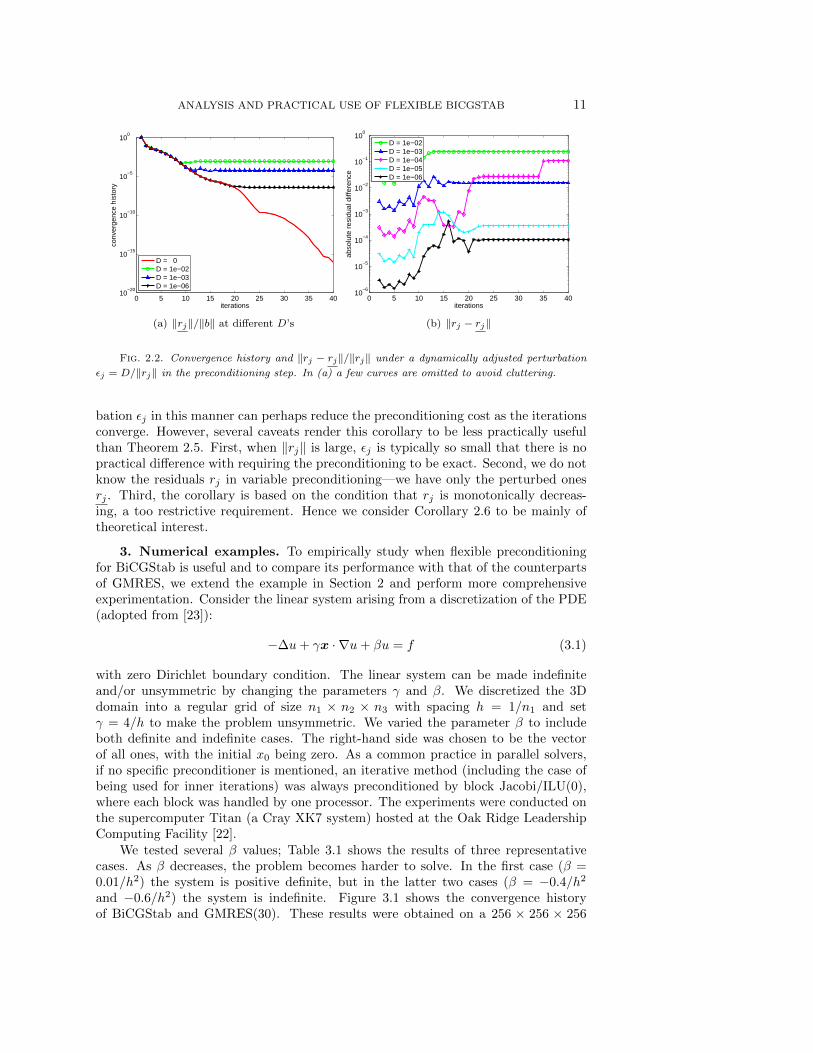
The absolute difference, ‖rj − rj‖, on the other hand, can be made bounded as

opposed to the increasing trends of Figure 2.1(b). One simple way is, in fact, todo nothing, because ‖rj‖ itself decreases. More interesting is that we can increase εacross iterations, as Corollary 2.6 implies. In Figure 2.2 we define εj = D/‖rj‖ forvarious different choices of D. The iterations converge to a level dependent on D.

One is tempted to infer from Corollary 2.6 that successively relaxing the pertur-


0 5 10 15 20 25 30 35 4010

−20

10−15

10−10

10−5

100

iterations

conv

erge

nce

hist

ory

D = 0D = 1e−02D = 1e−03D = 1e−06

(a) ‖rj‖/‖b‖ at different D’s

0 5 10 15 20 25 30 35 4010

−6

10−5

10−4

10−3

10−2

10−1

100

iterations

abso

lute

res

idua

l diff

eren

ce

D = 1e−02D = 1e−03D = 1e−04D = 1e−05D = 1e−06

(b) ‖rj − rj‖

Fig. 2.2. Convergence history and ‖rj − rj‖/‖rj‖ under a dynamically adjusted perturbation

εj = D/‖rj‖ in the preconditioning step. In (a) a few curves are omitted to avoid cluttering.

bation εj in this manner can perhaps reduce the preconditioning cost as the iterationsconverge. However, several caveats render this corollary to be less practically usefulthan Theorem 2.5. First, when ‖rj‖ is large, εj is typically so small that there is nopractical difference with requiring the preconditioning to be exact. Second, we do notknow the residuals rj in variable preconditioning—we have only the perturbed onesrj . Third, the corollary is based on the condition that rj is monotonically decreas-ing, a too restrictive requirement. Hence we consider Corollary 2.6 to be mainly oftheoretical interest.

3. Numerical examples. To empirically study when flexible preconditioningfor BiCGStab is useful and to compare its performance with that of the counterpartsof GMRES, we extend the example in Section 2 and perform more comprehensiveexperimentation. Consider the linear system arising from a discretization of the PDE(adopted from [23]):

−∆u+ γx · ∇u+ βu = f (3.1)

with zero Dirichlet boundary condition. The linear system can be made indefiniteand/or unsymmetric by changing the parameters γ and β. We discretized the 3Ddomain into a regular grid of size n1 × n2 × n3 with spacing h = 1/n1 and setγ = 4/h to make the problem unsymmetric. We varied the parameter β to includeboth definite and indefinite cases. The right-hand side was chosen to be the vectorof all ones, with the initial x0 being zero. As a common practice in parallel solvers,if no specific preconditioner is mentioned, an iterative method (including the case ofbeing used for inner iterations) was always preconditioned by block Jacobi/ILU(0),where each block was handled by one processor. The experiments were conducted onthe supercomputer Titan (a Cray XK7 system) hosted at the Oak Ridge LeadershipComputing Facility [22].

We tested several β values; Table 3.1 shows the results of three representativecases. As β decreases, the problem becomes harder to solve. In the first case (β =0.01/h2) the system is positive definite, but in the latter two cases (β = −0.4/h2

and −0.6/h2) the system is indefinite. Figure 3.1 shows the convergence historyof BiCGStab and GMRES(30). These results were obtained on a 256 × 256 × 256


grid using 16,384 processor cores. The relative residual tolerance and the maximumnumber of iterations were 1e-8 and 200, respectively.

0 50 100 150 20010

−10

10−8

10−6

10−4

10−2

100

102

iterations

rela

tive

resi

dual

BiCGStab, β = 0.01/h2

GMRES, β = 0.01/h2

BiCGStab, β = −0.4/h2

GMRES, β = −0.4/h2

BiCGStab, β = −0.6/h2

GMRES, β = −0.6/h2

Fig. 3.1. Convergence of BiCGStab and GMRES for three β’s (no inner iterations).

We compared BiCGStab, FBiCGStab/BiCGStab, GMRES, and FGMRES/GMRES,where FBiCGStab/BiCGStab means FBiCGStab is preconditioned by BiCGStab, andsimilarly for FGMRES/GMRES. In both of the flexible methods, the stopping cri-terion for the inner iterations was either a residual tolerance or a fixed number ofiterations. The two major comparison metrics are the number of matrix-vector multi-plications (MatMult, column 4) and the number of calls to MPI Allreduce (Allreduce,column 5). The number of floating point operations (Flops, column 6) for computingthe inner products is listed for reference, but it is not a fair criterion for comparisonbecause (i) the synchronization cost in MPI Allreduce is much higher than that offloating point operations, and (ii) GMRES requires long-term recurrence (orthogonal-ization) whereas BiCGStab does not. The wallclock time is also listed, but note thatthe fluctuations in a distributed memory computing environment and the communi-cation latency are factors that affect the actual running time.

Several observations are made according to Table 3.1 and other experiments withintermediate β values that are not shown in the table. First, for this set of testcases, the GMRES family in general performs better when the system is relativelyeasy to solve; but as the difficulty level increases, the BiCGStab family outperformsthe GMRES family. One sees that in the first case (β = 0.01/h2) GMRES is thebest solver, whereas in the second case it failed to converge to the required tolerancebut BiCGStab did converge. In the second case (β = −0.4/h2), however, the fastestsolver is still in the GMRES family. Nevertheless, when moving to the third case(β = −0.6/h2), FBiCGStab with an inner tolerance stopping criterion clearly winsover all other solvers. This interesting phenomenon indicates that even for the sameproblem, different solvers may have significantly different performance profiles as theproblem parameters vary.

Second, for a flexible Krylov method, using a fixed number of inner iterationscan sometimes achieve excellent performance; but as the problem becomes harder


Table 3.1Solution summary of (3.1) with three choices of β. Arrows point to the fastest run.

Outer TimeMatMult

Inner Productβ = 0.01/h2 Iter. (sec×10−1) Allreduce Flops×105BiCGStab 21 1.132 42 84 3.010FBiCGStab, inner rtol = 1e-3 2 1.397 58 120 4.246FBiCGStab, inner rtol = 1e-2 2 1.335 44 92 3.233FBiCGStab, inner rtol = 1e-1 4 1.364 54 116 4.037FBiCGStab, inner max it = 5 2 1.131 44 92 3.233FBiCGStab, inner max it = 10 1 1.147 40 82 2.910FBiCGStab, inner max it = 20 1 1.226 46 94 3.334GMRES 29 0.874 29 58 9.494 ←FGMRES, inner rtol = 1e-3 3 1.122 40 83 6.081FGMRES, inner rtol = 1e-2 4 7.200 37 78 4.240FGMRES, inner rtol = 1e-1 7 1.153 38 83 3.292FGMRES, inner max it = 5 6 1.072 36 78 3.130FGMRES, inner max it = 10 3 1.066 33 69 4.237FGMRES, inner max it = 20 2 1.065 40 82 8.720

β = −0.4/h2 ×100 ×106BiCGStab 105 0.356 210 420 1.505FBiCGStab, inner rtol = 1e-3 2 0.668 438 880 3.144FBiCGStab, inner rtol = 1e-2 2 0.499 270 544 1.948FBiCGStab, inner rtol = 1e-1 6 0.832 586 1184 4.225FBiCGStab, inner max it = 5 fail - - - -FBiCGStab, inner max it = 10 fail - - - -FBiCGStab, inner max it = 20 25 2.517 2050 4150 14.800GMRES fail - - - -FGMRES, inner rtol = 1e-3 3 1.556 1165 2298 37.890FGMRES, inner rtol = 1e-2 4 1.062 803 1586 25.550FGMRES, inner rtol = 1e-1 7 0.791 560 1113 17.160FGMRES, inner max it = 5 26 0.282 156 338 1.893FGMRES, inner max it = 10 14 0.278 154 322 2.134 ←FGMRES, inner max it = 20 12 0.373 252 516 5.861

β = −0.6/h2 ×101 ×107BiCGStab fail - - - -FBiCGStab, inner rtol = 1e-3 2 0.951 8314 16632 5.962FBiCGStab, inner rtol = 1e-2 2 0.572 5024 10052 3.605 ←FBiCGStab, inner rtol = 1e-1 15 3.564 30120 60270 21.560FBiCGStab, inner max it = 5 fail - - - -FBiCGStab, inner max it = 10 fail - - - -FBiCGStab, inner max it = 20 fail - - - -GMRES fail - - - -FGMRES, inner rtol = 1e-3 5 5.291 51670 101680 169.600FGMRES, inner rtol = 1e-2 5 4.589 41800 82259 136.560FGMRES, inner rtol = 1e-1 7 3.903 37757 74305 123.730FGMRES, inner max it = 5 fail - - - -FGMRES, inner max it = 10 fail - - - -FGMRES, inner max it = 20 fail - - - -


and harder, it is difficult to specify an appropriate number a priori to ensure theconvergence of the outer iterations. One sees that in the first case, using a fixednumber of inner iterations as the stopping criterion is in general preferable over usinga residual tolerance. This is also true in the second case for the FGMRES solvers;however, for the FBiCGStab solvers the situation is completely opposite. In the thirdcase, none of the solvers using a fixed number of inner iterations converged. In thissense, setting an inner tolerance is a more robust practice.

Third, one can choose an “optimal” inner tolerance for a flexible method. One seesthat for FBiCGStab the inner tolerance 1e-2 yields the best results in all the cases,whereas for FGMRES the tolerance is 1e-1. This is consistent with the observationmade in the experiments of flexible QMR [33], which states that the total solver costfirst decreases, then increases as the inner solves are more and more exact. The“optimal” inner tolerance may be related to the convergence behavior of the inneriterations. One sees that in Figure 3.1 the relative residual norm of BiCGStab hasa steep decrease at the beginning, until between 1e-1 and 1e-2. This may be thestopping point when BiCGStab becomes the most effective as an inner solve.

Fourth, the inner-outer iterations (that is, FBiCGStab/BiCGStab and FGM-RES/GMRES) are often a better alternative to the standard iterations (that is,BiCGStab and GMRES). In harder problems the standard iterations did not con-verge whereas the inner-outer iterations did. In fact, the outer iterations convergeextremely fast when an appropriate inner tolerance is used.

4. Application. In this section, we explore the use of flexible BiCGStab toimprove the run-time performance of a large-scale application, PFLOTRAN [17, 19],where historically standard BiCGStab with block Jacobi/ILU(0) preconditioner hasbeen the preferred linear solver. Based on the analysis in Section 2, we composea multigrid (MG) preconditioner. Its use with BiCGStab yields two to three timesimprovement in solution time onO(104)–O(105) processor cores. When the coarse gridsolver varies slightly (thus becoming a variable preconditioner and having to be usedwith FBiCGStab), we gain an additional 10–20% in overall runtime improvement.

PFLOTRAN is a state-of-the-art code for simulating multiscale, multiphase, mul-ticomponent flow and reactive transport in geologic media. It solves a coupled systemof mass and energy conservation equations for a number of phases, including air,water, supercritical CO2 and a number of chemical components. The code utilizesfinite volume or mimetic finite difference spatial discretizations and backward-Euler(fully implicit) timestepping. At each time step, Newton-Krylov methods are usedfor solving the resulting nonlinear algebraic equations. PFLOTRAN is built on thePETSc library [3, 4] and makes extensive use of PETSc iterative nonlinear and linearsolvers.

The governing equations are described by Richards’ equation:

∂

∂t

(ϕsρ

)+∇ · ρu = S,

where ϕ denotes the porosity of the geologic medium, s the saturation (fraction of porevolume filled with liquid water), ρ the fluid density, S a source/sink term representingwater injection/extraction, and u the Darcy velocity defined as

u = −κκrµ∇(P − ρgz

),

where P denotes fluid pressure, µ viscosity, κ the absolute permeability of the medium,


κr the relative permeability of water to air, g the acceleration of gravity, and z thevertical distance from a datum.

We consider two benchmark problems [18]:

Case 1: Cubic domain with a central injection well. This case models a 100m ×100m × 100m domain with a uniform effective permeability of 1 darcy andan injection well at the exact center.

Case 2: Regional flow without well near river. This case models a 5000m × 2500m× 100m region with a river at the eastern boundary.

In our numerical experiments, we ran each test case with a minimum number of timesteps—six for case 1 and two for case 2— at which the number of linear iterations perNewton step became stabilized.

BiCGStab preconditioned by block Jacobi/ILU(0) has been the preferred linearsolver for PFLOTRAN because of its small memory consumption, compared withthat of GMRES, and the empirically fast convergence. Similar to other Krylov meth-ods, however, as the size of the application and the number of processors increase,BiCGStab encounters a well-known scaling difficulty for over 10,000 processor coresbecause of the bottleneck in vector inner-product calculations. The synchronizationcost in MPI Allreduce for computing inner products can constitute more than halfof the solution time. In order to overcome the scaling difficulty, two algorithms wereexplored to successfully reduce the synchronization cost [18]. One was the use offlexible GMRES with a hierarchical GMRES preconditioner, where inner GMRESiterations are run on diagonal submatrices over subgroups of processor cores only.On each submatrix, inner GMRES is further preconditioned by block Jacobi/ILU(0).We denote this approach FGMRES/h-GMRES. The second algorithm was to use theIBiCGStab algorithm [39] with a Chebyshev preconditioner. We denote this approachto be IBiCGStab/Chebyshev. IBiCGStab is mathematically equivalent to BiCGStab,but the iterates are reorganized so that several inner products are computed togetherto reduce the number of synchronizations. The Chebyshev iterations may not be as ef-fective in reducing the condition number as other Krylov iterations, but an advantageis that it does not require any inner product calculations and thus can be used as afixed preconditioner. The two algorithms are based on the idea of reducing expensiveglobal inner products across the entire system by using cheaper local inner products(e.g., FGMRES/h-GMRES) or inner iterations that do not compute inner productsat all (e.g., IBiCGStab/Chebychev).

The success in [18] prompted us to explore similar ideas for BiCGStab. The firstattempt was to use BiCGStab in place of GMRES in FGMRES/h-GMRES, such asFBiCGStab/h-GMRES and FBiCGStab/h-BiCGStab. The use of a small constantnumber of inner iterations generally failed for convergence; the failure is not surprisingbecause a few iterations make the preconditioner vary too much, and FBiCGStab doesnot guarantee any form of outer convergence as does FGMRES (monotonic decreaseof residuals regardless of the varying of preconditioner). On the other hand, when weused an inner tolerance as the stopping criterion, convergence is seen for a reasonablychosen value (see Figure 4.1). In fact, the general trend for the same tolerance issimilar for whichever preconditioner is used, either h-GMRES or h-BiCGStab, andthe smaller the tolerance, the closer the residual history is to a fixed preconditionercase. However, this convergence was obtained at the cost of a large number of inneriterations. The overall run time cannot compete with the simple strategy of usingBiCGStab preconditioned by block Jacobi/ILU(0).

We therefore searched for a preconditioner that converges faster to the level of


0 20 40 60 80 10010

−7

10−6

10−5

10−4

10−3

10−2

10−1

100

outer iterations

abso

lute

res

idua

l diff

eren

ce

FBiCGStab/h−GMRES: 1.e−2FBiCGStab/h−BiCGStab: 1.e−2FBiCGStab/h−GMRES: 1.e−3FBiCGStab/h−BiCGStab: 1.e−3FBiCGStab/h−GMRES: 1.e−6FBiCGStab/h−BiCGStab: 1.e−6

Fig. 4.1. Convergence history of FBiCGStab/h-GMRES and FBiCGStab/h-BiCGStab forPFLOTRAN case 1 (mesh size 256× 256× 256) using 512 processor cores.

1e-2 to 1e-3. Among all preconditioners examined, we settled on multigrid witha particular choice of the smoothers and the coarse-grid solver. Multigrid (MG) isgenerally applicable to steady-state or close to steady-state problems, such as the twocases of PFLOTRAN we consider here. In the standard setting, multigrid is a fixedpreconditioner, because the smoothers (such as SOR or Chebyshev) require no inner-product calculations and the coarsest-grid problem is solved exactly by using a directlinear solver. In other words, one can, in principle, write down the linear operator forone cycle of multigrid and see that it does not vary.

For PFLOTRAN applications, the MG preconditioner was known to work wellon a small number of processors, but the performance started tailing off at around1,000 processor cores [16]. The difficulty to scale up the number of processors is thatin the coarsest level, the problem is so small that the communication cost outweighsthe computational cost. We cope with this difficulty by limiting the number of levels(effectively, three), such that the coarsest grid is not too small, and employing an itera-tive method to approximately solve the coarsest-grid problem. Two coarse grid solversare (1) 100 Chebyshev iterations, and (2) 5 IBiCGStab iterations, each preconditionedby 20 Chebyshev iterations. For the former, even though the coarsest-grid problem isnot solved to full accuracy, multigrid is still considered a fixed preconditioner becausethere are no inner product calculations. For the latter, clearly, multigrid is a variablepreconditioner.

We conducted experiments with the above ideas on two computer systems: In-trepid, an IBM Blue Gene/P supercomputer located at the Argonne Leadership Com-puting Facility [1], and Titan, a Cray XK7 system located at the Oak Ridge LeadershipComputing Facility [22]. Intrepid has 40,960 nodes, each consisting of one 850 MHzquad-core processor and 2GB RAM, resulting in a total of 163,840 cores, 80TB ofmemory, and a peak performance of 557 TFlops. Titan has 18,688 compute nodes,each consisting of one AMD 16-core Opteron 6274 processor running at 2.2GHz and32GB of memory, giving a total of 299,008 cores.


Table 4.1BiCGStab and FBiCGStab for PFLOTRAN on Intrepid (IBM Blue Gene/P), Case 1.

IBiCGS/Cheby BiCGStab/MG FBiCGStab/Variable MGSmoother: Cheby Smoother: Cheby

Number of Cores CSolve: Cheby CSolve: IBiCGS/Cheby(Mesh Size) Iter. Time Iter. Time Iter. Time (% Reduction)

512(256x256x256) 547 212.8 29 97.2 23 86.4 (11%)

4,096(512x512x512) 1006 365.1 43 121.3 33 106.1 (12%)

32,768(1024x1024x1024) 1886 654.3 62 153.7 37 119.1 (23%)

163,840(1600x1600x640) 2843 308.3 88 81.8 53 65.7 (20%)

Table 4.2BiCGStab and FBiCGStab for PFLOTRAN on Intrepid (IBM Blue Gene/P), Case 2.



16,384(1600x816x320) 844 231.1 33 64.3 22 52.6 (18%)

98,304(1600x1632x640) 1520 270.5 61 70.0 39 54.7 (22%)

163,840(1600x1632x640) 1499 169.3 62 52.0 36 40.2 (23%)

Tables 4.1 through 4.4 compare the performance of (1) IBiCGStab/Chebyshev,(2) BiCGStab with the fixed MG preconditioner, and (3) FBiCGStab with the variableMG preconditioner on the two benchmark cases. The results of IBiCGStab/Chebyshev(columns 2–3) have been reported in [18] and are used here as the baseline of compar-ison. For MG preconditioners (columns 4–8), V-cycle was used; the smoothers were 2steps of Chebyshev iterations because we found that Chebyshev outperformed otherchoices of smoothers. For both smoothers and coarse grid solvers, block Jacobi/ILU(0)was used as the innermost preconditioner.

Overall, FBiCGStab with an MG preconditioner is two to three times faster thanthe baseline IBiCGStab/Chebyshev on a large number of processor cores. Hence, thefocus of comparison here is how much reduction in execution time one can achieveby using a variable preconditioner compared with using a fixed one. The percentageof reduction in execution time relative to the fixed MG preconditioner is listed incolumn 8 (% Reduction). As the size of the problem (hence coarsest grid) increases,the fixed number of iterations used for the coarsest-grid solver weakens the MG pre-conditioner, resulting in an increased number of outer iterations. Such an increase isless significant for the variable MG preconditioner because IBiCGStab/Chebyshev ismore effective as a preconditioner than Chebyshev alone is. For example, when thenumber of cores becomes larger than 30,000, the number of outer iterations for usingthe variable MG preconditioner is almost half that of using the fixed MG precondi-tioner, leading to a reduction of 10% and 20% in overall execution time, on Titan and


Table 4.3BiCGStab and FBiCGStab for PFLOTRAN on Titan (Cray XK7), Case 1.



512(256x256x256) 546 24.2 29 13.5 23 12.5 (7%)

4,096(512x512x512) 1033 44.1 43 18.1 33 16.6 (8%)

32,768(1024x1024x1024) 2073 89.0 62 27.4 37 24.3 (11%)

160,000(1600x1600x640) 2407 52.0 91 24.9 55 22.5 (10%)

Table 4.4BiCGStab and FBiCGStab for PFLOTRAN on Titan (Cray XK7), Case 2.



1,600(800x408x160) 411 18.0 20 8.8 20 8.8 (0%)

16,000(1600x816x320) 829 29.6 30 11.3 22 10.9 (4%)

80,000(1600x1632x640) 1578 53.1 60 16.7 38 15.0 (10%)

224,000(1600x1632x640) 1501 20.9 66 16.6 37 14.8 (11%)

Intrepid, respectively.

Comparing the results obtained on the two machines, one sees a consistent iter-ation number (for some grid sizes, a slightly different number of processor cores wasused across machines; this affected the innermost block Jacobi/ILU(0), thus makingthe iteration numbers slightly different). However, the time improvement of using avariable MG preconditioner is very different across the two machines. Because theclock rate of Intrepid is much lower than that of Titan, the solution time on Intrepidis longer. However, the communication network of Intrepid has a lower latency, so theglobal synchronization cost of MPI Allreduce is smaller. We thus achieve better per-formance improvement on Intrepid because the variable MG preconditioner requiresinner product calculations in the coarsest-grid solves. This phenomenon is not rare inpractice. It showcases that for a solver, not only the theoretical convergence matters,but also the machine architecture plays an important role.

5. Concluding remarks. BiCGStab has been the de facto method of choice inmany application domains for solving linear systems. Motivated by the challenges inlarge-scale scientific applications and extreme-scale computer architectures that en-courage the use of variable preconditioners, we analyzed flexible BiCGStab and showedthat the change of the convergence behavior with respect to standard BiCGStab isin accordance with the inaccuracy of the preconditioning solves. Thus, often a stop-


ping criterion with a moderate tolerance, say 1e-4 to 1e-2, for the preconditioningsolves is favored in order both to maintain convergence and to reduce overall compu-tation time. To this end, we demonstrated through numerical experiments, includingthe PFLOTRAN reacting flow application, that FBiCGStab with variable precondi-tioning yields superior performance on extreme-scale computers. This work providesinsight on the practical use of FBiCGStab for large-scale applications.

Acknowledgments. We thank Satish Balay and Jed Brown for insightful dis-cussions and assistance with experiments. The authors were supported by the Officeof Advanced Scientific Computing Research, Office of Science, U.S. Department ofEnergy, under Contract DE-AC02-06CH11357.

REFERENCES

[1] ALCF, Intrepid Supercomputer. http://www.alcf.anl.gov/intrepid.[2] J. Ang, K. Evans, A. Geist, M. Heroux, P. Hovland, O. Marques, L. McInnes, E. Ng,

and S. Wild, Report on the workshop on extreme-scale solvers: Transitions to future ar-chitectures. Office of Advanced Scientific Computing Research, U.S. Department of Energy,2012. Washington, DC, March 8-9, 2012.

[3] S. Balay, J. Brown, K. Buschelman, V. Eijkhout, W. D. Gropp, D. Kaushik, M. G.Knepley, L. C. McInnes, B. F. Smith, and H. Zhang, PETSc users manual, Tech. Rep.ANL-95/11 - Revision 3.3, Argonne National Laboratory, 2012.

[4] S. Balay, W. D. Gropp, L. C. McInnes, and B. F. Smith, Efficient management of paral-lelism in object oriented numerical software libraries, in Modern Software Tools in ScientificComputing, E. Arge, A. M. Bruaset, and H. P. Langtangen, eds., Birkhauser Press, 1997,pp. 163–202.

[5] P. G. Bridges, K. B. Ferreira, M. A. Heroux, and M. Hoemmen, Fault-tolerant linearsolvers via selective reliability, CoRR, abs/1206.1390 (2012).

[6] J. Brown, M. G. Knepley, D. A. May, L. C. McInnes, and B. F. Smith, Composable linearsolvers for multiphysics, in Proceeedings of the 11th International Symposium on Paralleland Distributed Computing (ISPDC 2012), IEEE Computer Society, 2012, pp. 55–62. Alsoavailable as Argonne National Laboratory preprint ANL/MCS-P2017-0112.

[7] A. Chronopoulos and C. W. Gear, S-step iterative methods for symmetric linear systems,Journal of Computational and Applied Mathematics, 25 (1989), pp. 153–168.

[8] H. A. V. der Vorst and C. Vuik, GMRESR: a family of nested GMRES methods, NumericalLinear Algebra with Applications, 1 (1994), pp. 369–386.

[9] A. El maliki, R. Guenette, and M. Fortin, An efficient hierarchical preconditioner forquadratic discretizations of finite element problems, Numerical Linear Algebra with Appli-cations, 18 (2011), pp. 789–803.

[10] J. v. Eshof and G. L. G. Sleijpen, Inexact Krylov subspace methods for linear systems, SIAMJournal on Matrix Analysis and Applications, 26 (2004), pp. 125–153.

[11] R. Fletcher, Conjugate gradient methods for indefinite systems, Lecture Notes in Mathemat-ics, 506 (1976), pp. 73–89.

[12] P. Ghysels, T. Ashby, K. Meerbergen, and W. Vanroose, Hiding global communicationlatency in the GMRES algorithm on massively parallel machines, Tech. report 04.2012.1,Intel Exascience Lab, Leuven, Belgium, 2012.

[13] E. Giladi, G. H. Golub, and J. B. Keller, Inner and outer iterations for the Chebyshevalgorithm, SIAM J. Numer. Anal, 35 (1995), pp. 300–319.

[14] G. H. Golub and Q. Ye, Inexact preconditioned conjugate gradient method with inner-outeriteration, SIAM Journal on Scientific Computing, 21 (1999), pp. 1305–1320.

[15] D. E. Keyes, L. C. McInnes, C. Woodward, W. Gropp, E. Myra, M. Pernice, J. Bell,J. Brown, A. Clo, J. Connors, E. Constantinescu, D. Estep, K. Evans, C. Farhat,A. Hakim, G. Hammond, G. Hansen, J. Hill, T. Isaac, X. Jiao, K. Jordan, D. Kaushik,E. Kaxiras, A. Koniges, K. Lee, A. Lott, Q. Lu, J. Magerlein, R. Maxwell, M. Mc-Court, M. Mehl, R. Pawlowski, A. P. Randles, D. Reynolds, B. Riviere, U. Rude,T. Scheibe, J. Shadid, B. Sheehan, M. Shephard, A. Siegel, B. Smith, X. Tang,C. Wilson, and B. Wohlmuth, Multiphysics Simulations: Challenges and Opportunities,International Journal of High Performance Computing Applications, 27 (2013), pp. 4–83.


[16] B. Lee and G. Hammond, Parallel performance of preconditioned Krylov solvers for theRichards equation. Manuscript, 2010.

[17] P. Lichtner et al., PFLOTRAN project. http://ees.lanl.gov/pflotran/.[18] L. C. McInnes, B. Smith, H. Zhang, and R. T. Mills, Hierarchical and nested Krylov

methods for extreme-scale computing, Preprint ANL/MCS-P2097-0512, Argonne NationalLaboratory, 2012. submitted to Parallel Computing.

[19] R. T. Mills, V. Sripathi, G. Mahinthakumar, G. Hammond, P. C. Lichtner, and B. F.Smith, Engineering PFLOTRAN for scalable performance on Cray XT and IBM BlueGenearchitectures, in Proceedings of SciDAC 2010 Annual Meeting, 2010.

[20] M. Mohiyuddin, M. Hoemmen, J. Demmel, and K. Yelick, Minimizing communication insparse matrix solvers, in Proceedings of SC09, ACM, 2009.

[21] Y. Notay, Flexible conjugate gradients, SIAM Journal on Scientific Computing, 22 (2000),pp. 1444–1460.

[22] OLCF, Jaguar Supercomputer. https://www.olcf.ornl.gov/computing-resources/jaguar/.[23] Y. Saad, A flexible inner-outer preconditioned GMRES algorithm, SIAM Journal on Scientific

Computing, 14 (1993), pp. 461–469.[24] Y. Saad, Iterative Methods for Sparse Linear Systems, 2nd edition, SIAM, Philadelpha, PA,

2003.[25] Y. Saad and M. H. Schultz, GMRES: A generalized minimal residual algorithm for solving

nonsymmetric linear systems, SIAM J. Sci. Stat. Comput., 7 (1986), pp. 856–869.[26] Y. Saad and M. Sosonkina, pARMS: A package for the parallel iterative solution of general

large sparse linear systems user’s guide, Tech. Rep. UMSI2004-8, Minnesota Supercom-puter Institute, University of Minnesota, 2004.

[27] V. Simoncini and D. Szyld, Flexible inner-outer Krylov subspace methods, SIAM Journal onNumerical Analysis, (2003), pp. 2219–2239.

[28] V. Simoncini and D. B. Szyld, Theory of inexact Krylov subspace methods and applicationsto scientific computing, SIAM Journal on Scientific Computing, 25 (2003), pp. 454–477.

[29] G. L. Sleijpen, P. Sonneveld, and M. B. van Gijzen, Bi-CGSTAB as an induced dimensionreduction method, Applied Numerical Mathematics, 60 (2010), pp. 1100–1114.

[30] G. L. Sleijpen and M. B. van Gijzen, Exploiting BiCGstab(`) strategies to induce dimensionreduction, SIAM J. Sci. Comput., 32 (2010), pp. 2687–2709.

[31] P. Sonneveld and M. B. van Gijzen, IDR(s): A family of simple and fast algorithms forsolving large nonsymmetric systems of linear equations, SIAM Journal on Scientific Com-puting, 31 (2008), pp. 1035–1062.

[32] E. D. Sturler and H. A. van der Vorst, Reducing the effect of global communication inGMRES(m) and CG on parallel distributed memory computers, Applied Numerical Math-ematics, 18 (1995), pp. 441–459.

[33] D. B. Szyld and J. A. Vogel, FQMR: A flexible quasi-minimal residual method with inexactpreconditioning, SIAM Journal on Scientific Computing, 23 (2001), pp. 363–380.

[34] H. van der Vorst, BiCGSTAB: A fast and smoothly converging variant of BiCG for thesolution of nonsymmetric linear systems, SIAM J. Sci. Stat. Comput., 13 (1992), pp. 631–644.

[35] M. B. van Gijzen, G. L. Sleijpen, and J.-P. M. Zemke, Flexible and multi-shift induceddimension reduction algorithms for solving large sparse linear systems, Tech. Rep. 11-06,Delft University of Technology, 2011.

[36] J. van Rosendale, Minimizing inner product data dependencies in conjugate gradient itera-tion, in Proceedings of the IEEE International Conference on Parallel Processing, IEEEComputer Society, 1983.

[37] J. A. Vogel, Flexible BiCG and flexible Bi-CGSTAB for nonsymmetric linear systems, Ap-plied Mathematics and Computation, 188 (2007), pp. 226–233.

[38] R. Vuduc, Quantitative performance modeling of scientific computations and creating localityin numerical algorithms, PhD thesis, Massachusetts Institute of Technology, 1995.

[39] L. T. Yang and R. Brent, The improved BiCGStab method for large and sparse unsymmetriclinear systems on parallel distributed memory architectures, in Proceedings of the FifthInternational Conference on Algorithms and Architectures for Parallel Processing, IEEE,2002.

Government License. The submitted manuscript has been created by UChicagoArgonne, LLC, Operator of Argonne National Laboratory (“Argonne”). Argonne, aU.S. Department of Energy Office of Science laboratory, is operated under Contract


No. DE-AC02-06CH11357. The U.S. Government retains for itself, and others actingon its behalf, a paid-up nonexclusive, irrevocable worldwide license in said articleto reproduce, prepare derivative works, distribute copies to the public, and performpublicly and display publicly, by or on behalf of the Government.

analysis and practical use of flexible bicgstab 1. introduction. flexible iterative

Documents