analysis and interpretation of well test performance at ... · pdf filecondensate reservoir...

Copyright 1999, Society of Petroleum Engineers Inc.

This paper was prepared for presentation at the 1999 SPE Annual Technical Conference andExhibition held in Houston, Texas, 3–6 October 1999.

This paper was selected for presentation by an SPE Program Committee following review ofinformation contained in an abstract submitted by the author(s). Contents of the paper, aspresented, have not been reviewed by the Society of Petroleum Engineers and are subject tocorrection by the author(s). The material, as presented, does not necessarily reflect any positionof the Society of Petroleum Engineers, its officers, or members. Papers presented at SPEmeetings are subject to publication review by Editorial Committees of the Society of PetroleumEngineers. Electronic reproduction, distribution, or storage of any part of this paper for commercialpurposes without the written consent of the Society of Petroleum Engineers is prohibited.Permission to reproduce in print is restricted to an abstract of not more than 300 words;illustrations may not be copied. The abstract must contain conspicuous acknowledgment of whereand by whom the paper was presented. Write Librarian, SPE, P.O. Box 833836, Richardson, TX75083-3836, U.S.A., fax 01-972-952-9435.

AbstractThis paper presents a comprehensive field case history of theanalysis and interpretation of all of the available well test datafrom the giant Arun Gas Field (Sumatra, Indonesia). Arun Fieldhas estimated recoverable reserves on the order of 18-20 TCFand has 110 wells—78 producers, 11 injectors, 4 observationwells, and 17 abandoned. Approximately 100 well tests havebeen performed, and the analysis and interpretation of these datasuggests strong existence of condensate accumulation near thewellbore as well as a "regional pressure decline" effect causedby competing production wells.

We demonstrate and discuss the analysis/interpretation tech-niques for wells that exhibit condensate banking and non-Darcyflow. We found that the 2-zone radial composite reservoirmodel is effective for diagnosing the effects of condensate bank-ing at Arun Field.

We also demonstrate the development and application of anew solution for the analysis and interpretation for wells thatexhibit "well interference" effects. Our new solution treats the"interference effect" as a regional pressure decline and thisproposed solution accurately represents the well interferenceeffects observed in many of the well tests obtained at ArunField. Furthermore, this solution is shown to provide a muchbetter interpretation of well test data from a multiwell reservoirsystem than the existing approaches–i.e., assumption of no-flowor constant pressure boundaries, data truncation, etc.

IntroductionThe objective for performing well test analysis at Arun Field isto provide information regarding flow properties (e.g. permea-bility, near-well skin factor, and the non-Darcy flow coefficient)as well as the radial extent of condensate banking around thewellbore. As the reservoir pressure at Arun Field has declined

below the dew point (pdew=4,200 psia), these data are quitevaluable as an aid for estimating well deliverability and forassessing the need for well stimulation. Well test analyses arealso useful for general reservoir management activities such asinjection balancing and optimizing the performance of singleand multiple wells.

For the analysis of well test data, we use the single-phase gaspseudopressure approach–as this method does not require know-ledge of relative permeability data and it is much more conven-ient (and practical). The use of the single-phase pseudopressureapproach is justified by the concept that most of the reservoir is(or at least until recently, was) at pressures above the dew point.Further, any multiphase pseudopressure approach will requireknowledge of a representative relative permeability data set, aswell as a pressure-saturation function that is used to relatepressure and mobility (i.e., relative permeability).

The combined approach of using the single-phase gaspseudopressure coupled with a homogeneous reservoir model forthe analysis well performance in gas condensate reservoir hasbeen documented.1-4 This particular approach yields an accurateestimate of kh (the permeability-thickness product)–however, theestimated skin factor is much higher than the actual (near-well)skin factor. This "high skin" phenomenon occurs because thereis an accumulation of condensate liquid in the near-well regionthat behaves like second, lower permeability "reservoir" aroundthe wellbore. To resolve this problem, a 2-zone radial compositereservoir model is used, where the inner zone represents the"condensate bank," and the outer zone represents the "dry gasreservoir." The application of the 2-zone radial compositereservoir model for the analysis of well test data from a gascondensate reservoir was demonstrated by Raghavan, et al,3 andthen by Yadavalli and Jones.4

We use the 2-zone radial composite reservoir model in ouranalysis if we observe a distinct inner zone (due to con-densatebanking) in the well test data. This approach provides us withestimates of:

l Effective permeability to gas in both the "condensatebank," and in the "dry gas" reservoir,

l Mechanical skin factor,l Radial extent of condensate banking,

In some (often many) cases, wellbore storage masks the innerregion and affects our ability to obtain a complete suite of re-sults. In such cases, we only obtain an estimate of the total skinfactor. For the purpose of well stimulation (our objective is to

SPE 56487

Analysis and Interpretation of Well Test Performance at Arun Field, IndonesiaT. Marhaendrajana, Texas A&M U., and N.J. Kaczorowski, Mobil Oil (Indonesia), and T.A. Blasingame, Texas A&M U.

2 T. Marhaendrajana, N.J. Kaczorowski, and T.A. Blasingame SPE 56487

maximize well productivity ), knowledge of the total skin factoris useful.

Another phenomenon that we have observed at Arun Field isthe so-called "well interference" effect–which potentially leadsus to misinterpret well test data. In fact, many of the well testcases taken at Arun Field show this behavior–this well inter-ference effect tends to obscure the radial flow response, andhence, influence our analysis and interpretation efforts.

The first attempt to provide a generalized approach for theanalysis of well test data from multiwell reservoir systems waspresented by Onur et.al.5 The application of their method islimited as it assumes that all of the wells in question produce atthe same time and that the pseudosteady-state flow condition isachieved prior to shut-in. Arun Field has been produced for over20 years and currently in "blowdown" mode–we can assume thatthe reservoir is at currently at pseudosteady-state flow condi-tions).

Drawdown and buildup tests induce local transient effects–which are controlled by the reservoir and near-well permeability,the skin factor, and the non-Darcy flow coefficient–but not thereservoir volume. Most of the well tests performed at ArunField are relatively short (< 5 hours producing time), and thepseudosteady-state flow condition is not established in the areaof investigation given such short production times.

To address this issue we have developed a new method forthe analysis of well test data from a well in multiwell reservoirwhere we treat the "well interference" effect as a "RegionalPressure Decline." We note numerous cases of pressure builduptests taken at Arun Field where the pressure actually declines atlate times during the test–indicating communication with thesurrounding wells that are still on production.

Our new approach employs a straight-line graphical analysisof data on a Cartesian plot (∆te(d∆p/d∆te ) versus ∆t2/∆te )–wherethis yields a direct estimation of permeability. We have calledthis the "well interference" plot. The multiwell model used toderived this approach also allows us to use type curve andsemilog analysis–where "corrected" data functions are generatedusing the new "well interference" model proposed in the nextsection.

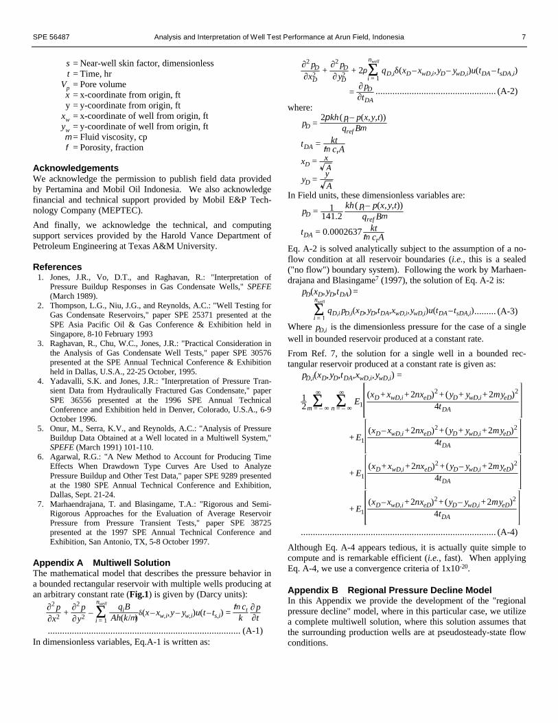
New Technique for the Analysis of Well Test Data in aMultiwell Reservoir SystemMultiwell Model. In our new solution we assume a boundedhomogeneous rectangular reservoir, with an arbitrary number ofwells, positioned at arbitrary locations (as shown in Fig. 1). Wealso assume a single compressible fluid phase, but we allow anyrate or pressure condition to be imposed at the well. However,our efforts in this work are focused on the constant flowratecase. The general analytical solution for the constant rate case isgiven by:

pD(xD,yD,tDA) =

qD,i pD,i(xD,yD,tDA,xwD,i,ywD,i)u(tDA – tsDA,i)Σi = 1

nwell

................ (1)

The derivation of Eq. 1 is given in Appendix A. This solution isvalid for all flow regimes (e.g., transient and boundary-domi-nated flow) and its computation is extremely rapid.

We have provided an extensive validation of this new solu-tion using numerical simulation for the case of square reservoirwith nine wells. For purposes of demonstration (not actualapplication), all wells are produced from the same starting timeand produce at the same constant rate. The dimensionless pres-sure and pressure derivative functions from both the analyticaland numerical solutions are plotted versus the dimensionlesstime function in Fig. 2. The open circles are the results fromnumerical simulation and the lines are the results from the newanalytical solution. We note that these solutions are identical–which validates our new analytical solution, at least concept-ually, as a mechanism to analyze well performance behavior in amultiwell reservoir system.

Regional Pressure Decline Model. To perform an analysis ofwell test data in a multiwell reservoir system, we must accountfor the "well interference" effects caused by offset productionwells. Our approach is to consider this interference as a"Regional Pressure Decline," where this pressure drop actsuniformly in the area of investigation.

Our "well interference" model assumes that all of the wells inthe reservoir are at pseudosteady-state flow conditions at thetime the "focus" well is shut-in. After shut-in, the reservoir inthe vicinity of the focus well will experience a significantpressure transient effect, but the offset wells remain onproduction. In simple terms, we assume that any rate change atthe focus well (including a drawdown/buildup sequence) haslittle effect on the offset wells. However, these offset producingwells will eventually have a profound effect on the wellperformance at the focus well–including, as we noted fromobservations at Arun Field, the flattening and decline of apressure buildup trend taken at the focus well.

The analytical solution for the focus well in this particularscenario is: (the details are provided in Appendix B)

pwD(tDA) = pD,1([xwD,1 + ε],[ ywD,1+ ε],tDA,xwD,1,ywD,1)

+ 2πtDA(αD – 1).................................................... (2)

where: αD =Vpct

q1Bd pdt =

Vpct

q1Bα

Where: ε = rwD/ 2 and rwD = rw/ A . pD,1(xD,yD,tDA,xwD,1,ywD,1)is the constant rate, single well solution for well 1 (i.e., the focuswell) and is given by Eq. A-4.

We have shown in Appendix C that the early-time pressurebuildup equation (in [pws-pwf(∆t=0)] format) derived from Eq. 2can be written as:

psD(∆tDA) + 2π(αD– 1)∆tDA = 12

ln 4eγ ∆tDAe

Arw

2 + s ......... (3)

Where ∆tDAe is given by:

∆tDAe =∆tDA tpDA

∆tDA + tpDA.................................................... (4)

The derivative formulation of Eq. 3 is given by:

∆tDAed psD

d∆tDAe= 1

2 – 2π (αD –1)∆tDA

2

∆tDAe............................. (5)

Eq. 5 suggests that a Cartesian plot of ∆tDAe(dpsD/d∆tDAe) vs.∆tDA

2 /∆tDAe will form a straight-line trend. Furthermore, semilogplot of psD+2π∆tDA(αD-1) versus ∆tDAe forms a straight line,

SPE 56487 Analysis and Interpretation of Well Test Performance at Arun Field, Indonesia 3

where this trend can be used to estimate formation permeabilityand skin factor.

To validate Eqs. 3 and 5, we use our new analytical solution(Eq. 1) for the case of a homogeneous, rectangular reservoirconsisting of nine wells with a uniform well spacing (see insetschematic diagram in Fig. 3). Our focus well is the center wellin this configuration. In this validation scenario, all wells exceptthe focus well are put on production at the same time and at thesame constant flowrate–are produced long enough to achievepseudosteady-state flow conditions.

Once this occurs, the focus well is then put on production forvarious producing times to simulate various case of pressuredrawdown (tpDA = 10-5, 10-4, 10-3, 10-2 respectively—where thedimensionless time in this comparison is based on total reservoirarea). All of the other producing wells are left on productionand the focus well is shut-in for a buildup test sequence. Thecase of single well in a reservoir of equal volume is alsoconsidered for comparison and discussion.

The pressure derivative responses for the focus well (forvarious producing times, tp) are plotted for the pressure buildupcases using ∆tDA(dpsD/d∆tDA) versus ∆tDA as shown in Fig. 3.This plotting function was originally proposed by Onur et.al5 asa means for estimating reservoir volume from a pressure builduptest. The data for the multiwell case are denoted by symbols andthe data for the single well case are given by the solid lines.

We note that the data from the single well case approacheszero as shut-in time increases–this is a distinct characteristic of a"no-flow" boundary. On the other hand, the data from the multi-well case decrease linearly to negative values as shut-in timeincreases–i.e., there is no "approaching zero" behavior. Thisbehavior is an indication of "well interference," i.e., the produc-ing wells dominate the behavior of the reservoir system, andhence, the behavior of the "focus" well.

On Figs. 4 and 5 we provide plots of the ∆tDAe(dpsD/d∆tDAe)function versus ∆tDA

2 /∆tDAe as suggested by Eq. 5. These figures(Fig. 4 is in semilog format, and Fig. 5 is in Cartesian format)show that the data for the multiwell cases follow a straight linepredicted by Eq. 5 (this is shown most clearly on Fig. 5). Theslope of this line is proportional to the rate of change of theaverage reservoir pressure at the time of shut-in for the focuswell.

For all cases, we note the general horizontal pressure deriva-tive behavior (i.e., the 0.5 line) as prescribed by Agarwal6 fortransient radial flow. The effect of the closed boundary (i.e., thepressure derivative function decaying to zero) is only apparentat very late times. Figs. 4 and 5 can be used as diagnostic toolsto identify the effect of well interference on pressure buildup testbehavior in a multiwell reservoir system.

Analysis Relations for Multiwell ReservoirsWe would like to develop a method for the analysis of pressurebuildup test data from a well in a multiwell reservoir system thatexhibits "well interference" effects. With that objective stated,we immediately note that Eq. 5 can be rearranged to obtain:

∆tDAed psD

d∆tDAe+ 2π (αD– 1)

∆tDA2

∆tDAe= 1

2................................. (6)

We propose Eq. 6 as a new plotting function for the pressurederivative function–where this relation specifically accounts forthe effects of well interference.

In Fig. 6 we plot the various pressure derivative functionsversus shut-in time or effective shut-in time. The solid linesdenote the single well approach (including the well interferenceeffects (there is no correction)) while the symbols denote themultiwell approach (correcting for the well interference effect assuggested by Eq. 6). We find that the multiwell approach yieldsa more clear (and longer) 0.5 line for the pressure derivativefunction.

In Fig. 7, we show that when we plot psD+2π∆tDA(αD-1)versus ∆tDAe on a semilog scale we obtain a much better semilogstraight line trend than simply plotting psD versus ∆tDAe. Thisobservation (as well as the general multiwell result (Eq. 6)),proves that we must take into account the effect of other pro-ducing wells in the analysis of pressure buildup test data in amultiwell reservoir system.

In Appendix C we provide Eqs. 3 and 5 in terms of fieldunits. These results are given as:

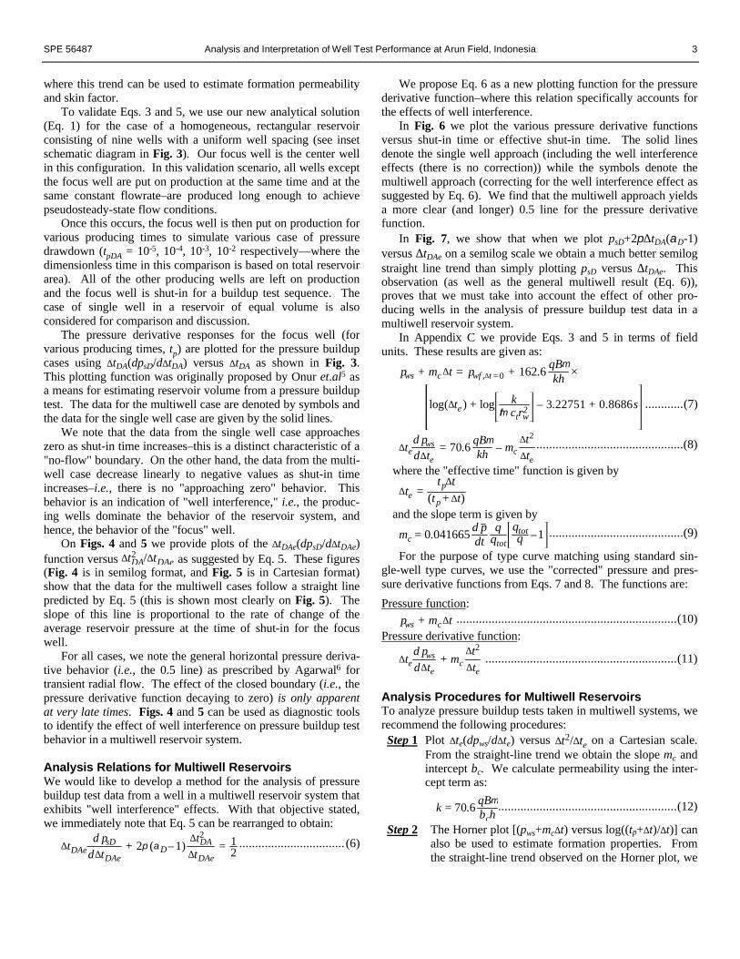
pws + mc ∆t = pwf ,∆t = 0 + 162.6qBµkh ×

log(∆te ) + log kφµctrw

2 – 3.22751 + 0.8686s ............(7)

∆ted pws

d∆te= 70.6

qBµkh

– mc∆t2

∆te..............................................(8)

where the "effective time" function is given by

∆te =tp∆t

(tp+∆t)and the slope term is given by

mc = 0.041665d pdt

qqtot

qtotq –1 ..........................................(9)

For the purpose of type curve matching using standard sin-gle-well type curves, we use the "corrected" pressure and pres-sure derivative functions from Eqs. 7 and 8. The functions are:

Pressure function:pws + mc ∆t .....................................................................(10)

Pressure derivative function:

∆ted pws

d∆te+ mc

∆t2

∆te............................................................(11)

Analysis Procedures for Multiwell ReservoirsTo analyze pressure buildup tests taken in multiwell systems, werecommend the following procedures:Step 1 Plot ∆te(dpws/d∆te) versus ∆t2/∆te on a Cartesian scale.

From the straight-line trend we obtain the slope mc andintercept bc. We calculate permeability using the inter-cept term as:

k = 70.6qBµbch

........................................................(12)

Step 2 The Horner plot [(pws+mc∆t) versus log((tp+∆t)/∆t)] canalso be used to estimate formation properties. Fromthe straight-line trend observed on the Horner plot, we


obtain the slope msl as well as the intercept term,( pws+mc∆t)∆t=1hr . Permeability is estimated using:

k = 162.6qBµmslh

..................................................... (13)

And the skin factor is calculated using:

s = 1.1513( pws +mc ∆t)∆t=1hr – pwf ,∆t = 0

msl

– 1.1513 logt p

t p+1 + log kφµctrw

2 –3.22751 ...... (14)

Step 3 In order to use standard single-well type curves fortype curve matching, we must make the appropriate"corrections" given by Eqs. 10 and 11. These relationsare:

Pressure function:pws + mc∆t .......................................................... (10)


∆ted pws

d∆te+ mc

∆t2

∆te................................................ (11)

Analysis of Pressure Buildup Test from Arun FieldIn this section we discuss our analysis and interpretation ofselected pressure buildup cases taken from the Arun Gas Field inSumatra, Indonesia. We provide a wide range of examples,where the examples shown exhibit some type of "well interfer-ence" effects, as well as the effect of condensate banking(several cases).

Recall that we have analyzed and interpreted approximately 100well tests from the Arun Field. Our goal is to identify cases thatclearly illustrate certain types of behavior–in particular:

l Effects of non-Darcy flow (not as prevalent).l Condensate banking (2-zone radial composite model).l "Well interference"/boundary effects.

The following well test cases are presented:

l Well C-I-18 (A-096) [Test Date: 28 Sep 1992]l Well C-II-15 (A-040) [Test Date: 26 May 1993]l Well C-IV-11 (A-084) [Test Date: 05 Jan 1992]l Well C-IV-11 (A-084) [Test Date: 04 May 1992]l Well C-IV-16 (A-051) [Test Date: 16 Mar 1993]l Well C-IV-16 (A-051) [Test Date: 16 Sep 1993]

Orientation for the Analysis/Interpretation Sequence:

Our analysis and interpretation of each well test case centers onthe following plot sequence

Test Summary Plot–We use a log-log plot of thepseudopressure drop (∆pp) and pseudopressure derivative(∆pp') functions versus the effective shut-in pseudotimefunction (∆tae). This plot includes the analysis resultsand the simulated test performance using these analysisresults. The primary value of this plot is the visual-ization of the pseudopressure derivative function, and the

corresponding flow regimes (and reservoir features) en-countered during a test.

Horner Plot–We also use a "Horner" semilog plot of theshut-in pseudopressure function, ppws, in order to providethe "conventional" semilog analysis of a particular dataset. We typically provide the semilog trends for the"inner" and "outer" regions corresponding to the con-densate and dry gas portions of the reservoir(respectively), for cases where both characteristics areobserved.

Muskat Plot–The "Muskat" plot is a relatively newapproach for establishing/confirming boundary-domi-nated flow behavior during a pressure buildup testsequence.7 We use a Cartesian plot of the shut-inpseudopressure function, ppws, versus the base derivativefunction, dppws/∆ta. This plot provides an extrapolationto the average reservoir pressure (or in this case, pseudo-pressure), based on the principle that the pseudopressureand pseudopressure derivative functions are representedby a single term exponential function.

"Well Interference" Plot–The "well interference" plot isa new approach for verifying the "regional pressuredecline" behavior associated with producing wells in amultiwell reservoir. This approach uses a Cartesian plotof the pseudopressure derivative (∆pp') function versusthe shut-in pseudotime group (∆ta

2/∆tae ). The slope of theresulting straight line (if a straight line exists) is used to"calibrate" the multiwell pressure and pressure derivativecorrection functions (Eqs. 10 and 11, respectively).

Well C-I-18 (A-096) [Test Date: 28 September 1992]. Thecorresponding figures showing our analysis for this case areprovided in Figs. 8 to 11. Well C-I-18 (A-096) was completedin June 1991 and had an initial pressure of approximately 3173psia at the time of completion. The results for this case are sum-marized in Table 1.

Test Summary Plot–Fig. 8 clearly shows the condensatebanking phenomena, as the pseudopressure derivativeexhibits 2 distinct horizontal trends. The raw derivativedata appear show a reservoir boundary, while the cor-rected derivative data show a continuance of the infinite-acting reservoir behavior (which is a result of our newmultiwell correction function).

Horner Plot–Fig. 9 verifies the condensate banking witha semilog straight line for the condensate bank as well asthe dry gas portion of the reservoir. This plot also showsan apparent reservoir boundary at late times.

Muskat Plot–The Muskat plot provided in Fig. 10 showsa reasonable straight-line trend at late times (to the left ofthe plot). However, this plot also shows a deviationfrom the expected linear trend at very late times, wherethis behavior prompts us to suggest that the nearbyproducing wells have caused a specific interferenceeffect.


An argument could be made that the derivative functionitself is the cause–as the derivative algorithm can skewthe derivative values near the end-points. While plaus-ible, we suggest that the nearby producing wells are themost likely cause of the "well interference" effects.

"Well Interference" Plot–Fig. 11 exhibits a slightly scat-tered, but clearly linear trend. This observation validatesour previous suggestion that deviation of the derivativefunction at late times is due to well interference fromsurrounding production wells. Our new multiwellreservoir model uniquely predicts this behavior.

Well C-II-15 (A-040) [Test Date: 26 May 1993]. Well C-II-15(A-040) was completed in January 1981 and had an initial pres-sure of approximately 6444 psia at the time of completion. Theresults for this case are summarized in Table 2.

Test Summary Plot–In Fig. 12, the pseudopressure deri-vative function clearly shows the condensate bankingphenomena, as well as a closed reservoir boundary (rawdata). The corrected derivative data (although a bitscattered at very late times) suggests the continuation ofthe infinite-acting radial flow regime.

Horner Plot–In Fig. 13 the shut-in pseudopressurefunction clearly indicates the presence of condensatebanking (note the two semilog straight-line trends). Thecondensate bank feature appears to dominate most of thewell performance behavior.

Muskat Plot–The Muskat plot in Fig. 14 shows a rela-tively good linear trend at late times and tends to confirmthe presence of a "closed boundary" feature.

"Well Interference" Plot–In Fig. 15 we note a reasonablywell defined linear trend, although there is considerablescatter at very late times. Using this trend, we find thatthe corrected functions in Fig. 12 (the log-log plot) dosuggest infinite-acting radial flow behavior.

Well C-IV-11 (A-084) [Test Date: 05 Jan 1992]. Well C-IV-11 (A-084) was completed in Arun Field in August 1990 andhad an initial pressure of approximately 3835 psia at the time ofcompletion. The results for this case are summarized in Table 3.

Test Summary Plot–Fig. 16 provides a log-log plot ofthe pseudopressure functions where the effect of conden-sate banking is not obvious, but a large wellbore storage/skin factor "hump" is observed in the pseudopressurederivative function. As is typical at Arun Field, theredoes appear to be the influence of a closed reservoirboundary at very late times (uncorrected data).

Horner Plot–The Horner plot shown in Fig. 17 gives aresponse that one would expect from a well in an in-finite-acting homogeneous reservoir. There are no ob-vious/apparent features resembling condensate bankingor reservoir boundaries.

Muskat Plot–The Muskat plot in Fig. 18 exhibits a fairlywell-defined linear trend at late times, confirming thepresence of a "closed boundary" feature.

"Well Interference" Plot–In Fig. 19 we observe a rela-tively consistent linear trend in the data, and concludethat well interference efforts are a possible mechanism.However, this trend only approaches zero, and does notactually extend to negative values, which is one criteriaassociated with the well interference model.

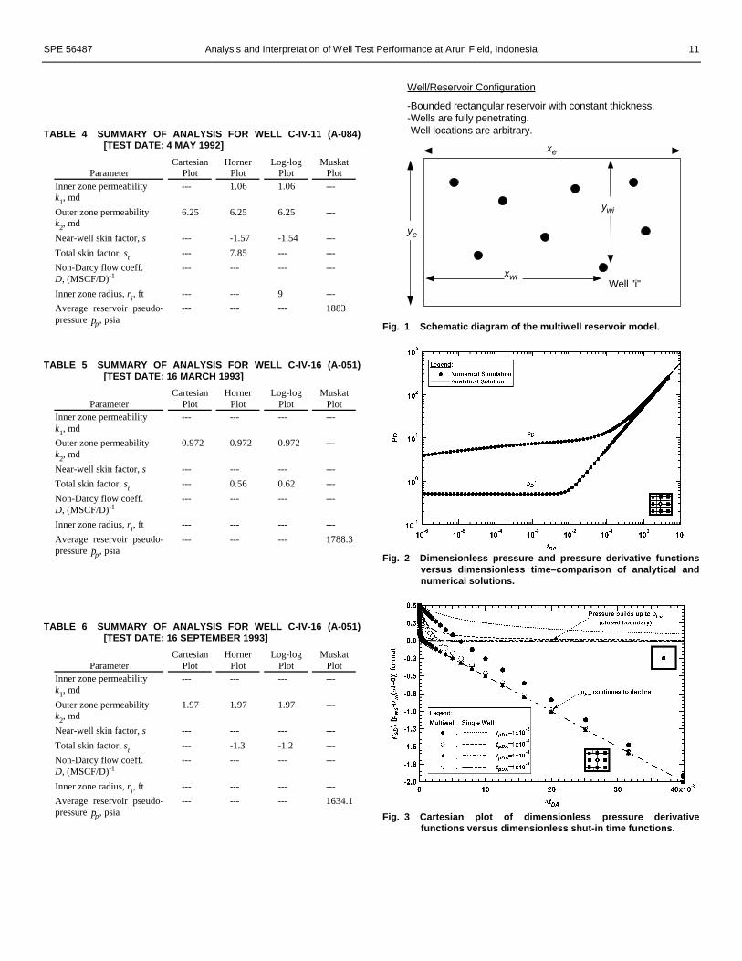
Well C-IV-11 (A-084) [Test Date: 04 May 1992]. This is an-other well test performed on Well C-IV-11 (A-084) on 4 May1992 and the results for this case are summarized in Table 4.The purpose of this test was to evaluate the effectiveness of anacid fracturing treatment performed in January 1992.

Test Summary Plot–Comparing the log-log summaryplot for this case (Fig. 20) with that of the previous test(Fig. 16), we immediately note a significantly smaller"hump" in the derivative function, suggesting that thewell has been substantially stimulated. We note that theflowrate prior to this test is to the pre-stimulation test isabout half that of the present test, but the maximumpseudopressure change at late times for the pre-stimula-tion test is almost twice that for the present test.

From Fig. 20 we conclude that the effect of condensatebanking is fairly modest, with only a slight "tail" in thepseudopressure derivative function. A boundary featureis apparent at very late times and the raw data again sug-gest that this is a closed boundary feature, while the"corrected" data indicate infinite-acting radial flow.

Horner Plot–We note two apparent semilog straight linetrends on the Horner plot shown in Fig. 21. Both trendswere constructed using the permeability values estimatedfor the "inner" (condensate) and "outer" (dry gas)regions. These trends appear to be reasonable, andshould be considered accurate.

Muskat Plot–In Fig. 22 we present the Muskat plot forthis case and we note a very well-defined linear trend atlate times, the extrapolated average reservoir pseudo-pressure ( pp) is 1882.8 psia. For the pre-stimulation

case, we obtained a pp estimate of 1920.0 psia (Fig. 18).

"Well Interference" Plot–Fig. 23 provides the "wellinterference" plot for this case. Comparing the trend onthis plot with the pre-stimulation case (Fig. 19), we notea remarkable similarity in the estimated slopes of thedata–confirming that the character of the regional pres-sure distribution has not changed significantly.

Well C-IV-16 (A-051) [Test Date: 16 Mar 1993]. Well C-IV-16 (A-051) was completed in Arun Field in March 1985 and hadan initial pressure of approximately 5818 psia at the time of theoriginal completion. This well was "sidetracked" andrecompleted in mid-1989. The results for this case are providedin Table 5.

Test Summary Plot– In Fig. 24 we present the summarylog-log plot and we note a fairly well defined boundaryfeature. However, there are no obvious signs of conden-


sate banking–the estimated skin factor is low (0.62) andan excellent match of the data is obtained without usingthe 2-zone radial composite reservoir model.

Horner Plot–The Horner plot in Fig. 25 shows the"classic" character of a pressure buildup test performedon a well in an infinite-acting homogeneous reservoir,with only wellbore storage and skin effects present.Only a very slight deviation of the pseudopressure trendis seen at late times, where this behavior is presumed tobe a boundary effect.

Muskat Plot–In Fig. 26 we present the Muskat plot forthis case and we note an excellent straight-line trend atlate times (as would be expected). However, we alsonote that the very last data deviate systematically fromthis trend, suggesting the possibility of external in-fluences–i.e., the well interference effect.

"Well Interference" Plot–In Fig. 27 we immediatelyobserve a new feature, the systematic deviation of thederivative trend. In fact, it appears that two linear trendscould be constructed. We have elected to use the "ear-lier" trend as we have more confidence in these data(which are not influenced by "endpoint" effects in thederivative algorithm). However, either trend could beused, and perhaps an "average" trend should be used.

The point of this exercise is that we clearly observe theeffects of well interference, but we have no single ex-planation for this behavior. For example, the drainagepattern may be non-uniform, and/or wells beyond theimmediate vicinity could be affecting the pressure distri-bution in the area of the focus well.

Well C-IV-16 (A-051) [Test Date: 16 Sep 1993]. This is an-other well test performed on Well C-IV-16 (A-051) on 16 Sep-tember 1993 and the results for this case are summarized inTable 6. This well test was performed to evaluate the effective-ness of an acid fracturing treatment performed in May 1993.

Test Summary Plot–From the early time data in Fig. 28we note a feature in the pseudopressure derivative func-tion that appears to suggest fracture stimulation (or aleast a significant improvement in near-well communica-tion). This feature is not apparent in the previous test(see Fig. 24). The "raw" pressure derivative function inFig. 28 shows the apparent effect of a closed boundary atlate times, while the "corrected" data suggest radial flowin an infinite-acting homogeneous reservoir.

Horner Plot–In Fig. 29 we have the Horner plot for thiscase, where this particular plot does not provide anyevidence of flow impediments, and suggests (at very latetimes) that a boundary has been encountered.

Muskat Plot–The Muskat plot for this case is shown inFig. 30 and we note a well-defined linear trend at latetimes, although we observe (as in the pre-stimulationtest), that the last few points deviate systematically fromthe straight-line trend. The extrapolated average

reservoir pseudopressure ( pp) for this case is 1634.1

psia, while for the pre-stimulation case, we obtained a ppestimate of 1788.3 psia (Fig. 26).

"Well Interference" Plot–In Fig. 31 we present the "wellinterference" plot for this case and comparing the lineartrend on this plot with the trend for the pre-stimulationcase (Fig. 27), we find that the estimated slopes havechanged considerably. However, given the somewhatill-defined nature of the trends in both cases, we can onlyconclude qualitatively that the regional pressure distribu-tion has changed.

Summary and ConclusionsIn summary, we have developed a rigorous and coherentapproach for the analysis of well test data taken from multiwellreservoir systems. Using the appropriate (dry gas) pseudopres-sure and pseudotime transformations, as well as the 2-zoneradial composite reservoir model and the non-Darcy flow model,we have effectively analyzed all of the well test data taken fromArun Field.

We have also provided new insight into the effects of wellinterference in large multiwell reservoirs. The most innovativeaspect of this work is the development of the new multiwellsolution and corresponding analysis procedures. The mostpractical aspect of this work is the demonstration/validation ofthese multiwell analysis techniques for the majority of wells atArun Field.

The following conclusions are derived from this work:

l The new "multiwell" solution has been successfully de-rived and applied for the analysis of well test data takenfrom a multiwell reservoir system.

l The appearance of "boundary" effects in pressure build-up test data taken in multiwell reservoirs can be cor-rected using our new approach. Care must be taken soas not to correct a true "closed boundary" effect.

l The 2-zone radial composite reservoir model has beenshown to be representative for the analysis and inter-pretation of well test data from Arun Field (most wellsexhibit radial composite reservoir behavior).

l The effect of non-Darcy flow on pressure buildup testanalysis seems to be minor for the wells in Arun Field.Although not a focus of the present study, our analysisof the pressure drawdown (flow test) data appear to bemuch more affected by non-Darcy flow effects.

NomenclatureA = Area, ft2B = Formation volume factor, RB/MSCFct = Total compressibility, psi-1D = Non-Darcy Flow Coefficient, (MSCF/D)-1h = Thickness, ftk = Formation permeability, mdp = Pressure or pseudopressure, psiaq = Sandface flow rate, MSCF/D

rw = Wellbore radius, ft


s = Near-well skin factor, dimensionlesst = Time, hr

Vp = Pore volumex = x-coordinate from origin, fty = y-coordinate from origin, ft

xw = x-coordinate of well from origin, ftyw = y-coordinate of well from origin, ftµ = Fluid viscosity, cpφ = Porosity, fraction

AcknowledgementsWe acknowledge the permission to publish field data providedby Pertamina and Mobil Oil Indonesia. We also acknowledgefinancial and technical support provided by Mobil E&P Tech-nology Company (MEPTEC).

And finally, we acknowledge the technical, and computingsupport services provided by the Harold Vance Department ofPetroleum Engineering at Texas A&M University.

References1. Jones, J.R., Vo, D.T., and Raghavan, R.: "Interpretation of

Pressure Buildup Responses in Gas Condensate Wells," SPEFE(March 1989).

2. Thompson, L.G., Niu, J.G., and Reynolds, A.C.: "Well Testing forGas Condensate Reservoirs," paper SPE 25371 presented at theSPE Asia Pacific Oil & Gas Conference & Exhibition held inSingapore, 8-10 February 1993

3. Raghavan, R., Chu, W.C., Jones, J.R.: "Practical Consideration inthe Analysis of Gas Condensate Well Tests," paper SPE 30576presented at the SPE Annual Technical Conference & Exhibitionheld in Dallas, U.S.A., 22-25 October, 1995.

4. Yadavalli, S.K. and Jones, J.R.: "Interpretation of Pressure Tran-sient Data from Hydraulically Fractured Gas Condensate," paperSPE 36556 presented at the 1996 SPE Annual TechnicalConference and Exhibition held in Denver, Colorado, U.S.A., 6-9October 1996.

5. Onur, M., Serra, K.V., and Reynolds, A.C.: "Analysis of PressureBuildup Data Obtained at a Well located in a Multiwell System,"SPEFE (March 1991) 101-110.

6. Agarwal, R.G.: "A New Method to Account for Producing TimeEffects When Drawdown Type Curves Are Used to AnalyzePressure Buildup and Other Test Data," paper SPE 9289 presentedat the 1980 SPE Annual Technical Conference and Exhibition,Dallas, Sept. 21-24.

7. Marhaendrajana, T. and Blasingame, T.A.: "Rigorous and Semi-Rigorous Approaches for the Evaluation of Average ReservoirPressure from Pressure Transient Tests," paper SPE 38725presented at the 1997 SPE Annual Technical Conference andExhibition, San Antonio, TX, 5-8 October 1997.

Appendix AMultiwell SolutionThe mathematical model that describes the pressure behavior ina bounded rectangular reservoir with multiple wells producing atan arbitrary constant rate (Fig.1) is given by (Darcy units):

∂2 p∂x2 +

∂2 p∂y2 –

qiBAh(k/µ)

δ(x– xw,i,y– yw,i)u(t– ts,i)Σi = 1

nwell

=φµct

k∂ p∂t

................................................................................ (A-1)In dimensionless variables, Eq.A-1 is written as:

∂2 pD

∂xD2 +

∂2 pD

∂yD2 + 2π qD,iδ(xD – xwD,i,yD– ywD,i)u(tDA – tsDA,i)Σ

i = 1

nwell

=∂pD∂tDA

.................................................. (A-2)

where:

pD =2πkh ( pi – p(x,y,t))

qref Bµ

tDA = ktφµctA

xD = xA

yD =yA

In Field units, these dimensionless variables are:

pD = 1141.2

kh( pi– p(x,y,t))qref Bµ

tDA = 0.0002637 ktφµctA

Eq. A-2 is solved analytically subject to the assumption of a no-flow condition at all reservoir boundaries (i.e., this is a sealed("no flow") boundary system). Following the work by Marhaen-drajana and Blasingame7 (1997), the solution of Eq. A-2 is:

pD(xD,yD,tDA) =

qD,i pD,i(xD,yD,tDA,xwD,i,ywD,i)u(tDA – tsDA,i)Σi = 1

nwell

......... (A-3)

Where pD,i is the dimensionless pressure for the case of a singlewell in bounded reservoir produced at a constant rate.

From Ref. 7, the solution for a single well in a bounded rec-tangular reservoir produced at a constant rate is given as:

pD,i(xD,yD,tDA,xwD,i,ywD,i) =

12 E1

(xD + xwD,i+ 2nxeD)2 + (yD+ ywD,i+ 2myeD)2

4tDAΣn = – ∞

∞

Σm = – ∞

∞

+ E1

(xD– xwD,i +2nxeD)2 +(yD+ ywD,i +2myeD)2

4tDA

+ E1

(xD+ xwD,i +2nxeD)2 +(yD– ywD,i +2myeD)2

4tDA

+ E1

(xD– xwD,i +2nxeD)2 +(yD– ywD,i +2myeD)2

4tDA

................................................................................. (A-4)

Although Eq. A-4 appears tedious, it is actually quite simple tocompute and is remarkable efficient (i.e., fast). When applyingEq. A-4, we use a convergence criteria of 1x10-20.

Appendix BRegional Pressure Decline ModelIn this Appendix we provide the development of the "regionalpressure decline" model, where in this particular case, we utilizea complete multiwell solution, where this solution assumes thatthe surrounding production wells are at pseudosteady-state flowconditions.


This condition presumes that any rate change (e.g., a pressuredrawdown/buildup sequence) at the focus well will have verylittle effect on the surrounding production wells. Therefore, apressure drawdown or pressure buildup test will cause transientflow conditions only in the vicinity of the focus well–not in theentire reservoir. Given the short period of a well test comparedto the entire production history of the reservoir, this localtransient phenomena is a reasonable and logical assumption.

Our new "regional pressure decline" model is written as fol-lows (Darcy units):

∂2 p∂x2 +

∂2 p∂y2 –

q1BAh(k/µ)

δ(x– xw,1, y– yw,1) –qiB

Ah(k/µ)Σi = 2

nwell

=φµctk

∂ p∂t

.................................................................................(B-1)Writing Eq. B-1 in terms of dimensionless variables, we have

∂2 pD

∂xD2 +

∂2 pD

∂yD2 + 2πqD,1δ(xD– xwD,1, yD– ywD,1) + 2π qD,iΣ

i = 2

nwell

=∂pD∂tDA

.................................................................................(B-2)For the case of a no-flow outer boundary, the solution of Eq. B-2is given as:

pD(xD,yD,tDA) = pD,1(xD,yD,tDA,xwD,1,ywD,1) + 2πtDA qD,iΣi = 2

nwell

.................................................................................(B-3)Where pD,1(xD,yD,tDA,xwD,1,ywD,1) is the solution for the case ofa single well in a bounded rectangular reservoir producing at aconstant rate. This solution is given by Eq. A-4. Eq. B-3 is onlystrictly valid in the vicinity if the focus well (i.e., well 1) and isused solely to model the pressure-time performance at the focuswell.From material balance, we have:

d pdt =

qtotBVpct

................................................................(B-4)

Defining a new parameter, the "well interference" coefficient,αD, we obtain

αD =Vpct

q1Bd pdt

=Vpct

q1Bα

..............................................(B-5)

Substituting Eq. B-4 into Eq. B-3, and using the definition givenby Eq. B-5, we obtain:

pD(xD,yD,tDA) = pD,1(xD,yD,tDA,xwD,1,ywD,1) + 2πtDA(αD – 1)

.................................................................................(B-6)

The first term on right-hand-side of Eq. B-6 is the pressureresponse caused by well 1 (i.e., the focus well), and the secondterm is the pressure response due to the other active producingwells in the reservoir system.

Evaluating the pressure response at the focus well, we have:pwD(tDA) = pD,1([xwD,1 + ε],[ ywD,1+ ε],tDA,xwD,1,ywD,1)

+ 2πtDA(αD – 1).................................................(B-7)

where ε = rwD/ 2 and rwD = rw/ A .

Appendix CDevelopment of Pressure BuildupAnalysis Method in Multiwell SystemFor a pressure buildup test performed on the focus well (i.e.,well 1) after a period of constant rate production in the focuswell (with the surrounding production wells at pseudosteady-state flow conditions) the pressure at well 1 (i.e., the focus well)is given by:

pwD(tDA) = pD,1([xwD,1 + ε],[ ywD,1+ ε],tDA,xwD,1,ywD,1)– pD,1([xwD,1 + ε],[ywD,1 + ε],tDA – tpDA,xwD,1,ywD,1)

+ 2πtDA(αD – 1) ......................................... (C-1)From Eq. C-1, we can write the pressure buildup equation forwell 1 (in [pi-pws] format) as:

psD(∆t DA) = pwD(t pDA+∆t DA) – pwD(∆t DA)

– pD,1([xwD,1 + ε],[ywD,1 + ε],∆tDA,xwD,1,ywD,1)

+ 2π(αD – 1)(tpDA + ∆tDA)........................... (C-2)

We would like to use the [pws-pwf(∆t=0)] format for our pressurebuildup formulation, therefore we proceed as follows:

[ pws – pwf (∆t =0)] = [ pi – pwf (∆t = 0)] – [ pi – pws] .......... (C-3)Hence,

psD(∆tDA) = pwD(t pDA) – psD(∆tDA)............................ (C-4)Substituting Eqs. B-7 and C-2 into Eq. C-4, and rearranging, weobtain:

psD(∆tDA) =pD,1([xwD,1 + ε],[ywD,1+ ε],tpDA,xwD,1,ywD,1)

+2π(αD – 1) tpDA– pD,1([xwD,1 + ε],[ywD,1+ ε],tDA + tpDA,xwD,1,ywD,1)

+ pD,1([xwD,1+ε],[ywD,1+ε],∆tDA,xwD,1,ywD,1)

– 2π(αD – 1)(tpDA +∆tDA) .................................. (C-5)

Cancelling the similar terms, Eq. C-5 reduces to the following:

psD(∆tDA) = pD,1([xwD,1 + ε],[ ywD,1 + ε],tpDA,xwD,1,ywD,1)

– pD,1([xwD,1 + ε],[ ywD,1 + ε],tDA + tpDA,xwD,1,ywD,1)

+ pD,1([xwD,1 +ε],[ywD,1 +ε],∆tDA,xwD,1,ywD,1)

– 2π(αD – 1) ∆tDA ....................................... (C-6)Using Eq. A-4 for the pD,1 variable, we have

pD,1([xwD,1 + ε],[ywD,1 + ε],tDA,xwD,1,ywD,1) =

12 E1

(2xwD+ ε +2nxeD)2 +(2ywD+ ε +2myeD)2

4tDAΣn = – ∞

∞

Σm = – ∞

∞

+ E1(ε +2nxeD)2 +(2ywD + ε +2myeD)2

4tDA

+ E1(2xwD + ε +2nxeD)2 +(ε +2myeD)2

4tDA

+ E1(ε +2nxeD)2 +(ε +2myeD)2

4tDA

.............. (C-7)

The early time (i.e., small ∆t) approximation for Eq. C-7 is:


pD,1([xwD,1 + ε],[ywD,1 +ε],tDA,xwD,1, ywD,1) = 12 E1

2ε2

4tDA

.................................................................................(C-8)Inserting the definition of ε into Eq. C-8, we obtain

pD,1([xwD,1 + ε],[ywD,1+ ε],tDA,xwD,1,ywD,1) = 12 E1

14tDA

rw2

A

.................................................................................(C-9)Substituting Eq. C-9 into Eq. C-6, we have

psD(∆tDA) = 12 E1

14tpDA

rw2

A– 1

2 E11

4(tpDA + ∆tDA)rw

2

A

+ 12

E11

4∆tDA

rw2

A– 2π(αD–1)∆tDA.................(C-10)

Using the logarithmic approximation for the Exponential Inte-gral terms, we write Eq. C-10 as:

psD(∆tDA) = 12ln

4tpDAeγ

Arw

2 – 12ln

4(tpDA+ ∆tDA)eγ

Arw

2

+ 12ln

4∆tDAeγ

Arw

2 – 2π(αD– 1) ∆tDA ...............(C-11)

Collecting the logarithm terms in Eq. C-11, we have

psD(∆tDA) = 12ln 4

eγ

tpDA×∆tDA

(tpDA +∆tDA)Arw

2 – 2π(αD–1) tDA

...............................................................................(C-12)Rearranging Eq. C-12 we obtain:

psD(∆tDA) + 2π(αD – 1) ∆tDA = 12ln 4

eγtpDA×∆tDA

(tpDA + ∆tDA)Arw

2

= 12ln 4

eγ ∆tDAeArw

2 ..........(C-13)

The ∆tDAe function is very similar to the "effective" shut-in timeproposed by Agarwal.6 The difference being that ∆tDAe isdefined using dimensionless times based on the total drainagearea, A.

∆tDAe =t pDA×∆tDA

(t pDA + ∆tDA)

This is an intermediate result, when we reduce these relations tofield units, we will use the Agarwal effective shut-in time (∆te).

Including the near-well skin factor, Eq. C-13 becomes:

psD(∆tDA) + 2π(αD– 1)∆tDA = 12ln 4

eγ ∆tDAeArw

2 + s ......(C-14)

Equation C-14 suggests that plot of psD+2π∆tDA(αD-1) versuslog(∆tDAe) will form a straight line. Substituting the definition ofthe dimensionless variables (in terms of field units) into Eq. C-14, we obtain

1141.2

kh(pws – pwf ,∆t = 0)qBµ + 2π 0.0002637k∆t

φµctAqtotq –1 =

12 ln 4

eγ0.0002637k

φµctrw2

tp∆

(t +∆ )+ ...............(C-15)

Multiplying both sides of Eq. C-15 by 141.2qBµ/kh and substi-tuting the material balance relation, d p/dt=5.615qtotB/φhAct, wehave

pws+ 0.041665d pdt

qqtot

qtotq –1 ∆t =

pwf ,∆t = 0 + 162.6qBµkh ×

logtp∆t

(tp+∆t) + log kφµctrw

2 – 3.22751 + 0.8686s

............................................................................... (C-16)To determine coefficient of ∆t on the left-hand-side of Eq. C-16,we proceed by differentiating Eq. C-14 with respect to ∆tDA,which gives us the following result

∆tDAd psD

d∆tDA= 1

2tpDA

(tpDA + ∆tDA)– 2π ∆tDA (αD –1) ...... (C-17)

Multiplying both sides by (tpDA + ∆tDA)

tpDA

, we obtain

(tpDA + ∆tDA)

tpDA∆tDA

d psD

d∆tDA= 1

2 – 2π (αD –1)(tpDA + ∆tDA)

tpDA∆tDA

............................................................................... (C-18)Using the following identity in terms of ∆tDA and ∆tDAe, we have

∆tDAed psD

d∆tDAe=

tpDA∆tDA

(tpDA + ∆tDA)d psD

d∆tDA

d∆tDA

d∆tDAe

=tpDA∆tDA

(tpDA + ∆tDA)d psD

d∆tDA

(tpDA + ∆tDA)

tpDA

2

=(tpDA + ∆tDA)

tpDA∆tDA

d psD

d∆tDA................. (C-19)

Substituting Eq. C-19 in Eq. C-18, we obtain

∆tDAed psD

d∆tDAe= 1

2 – 2π (αD–1)(tpDA + ∆tDA)

tpDA∆tDA

or finally, we have

∆tDAed psD

d∆tDAe= 1

2– 2π (αD– 1)

∆tDA2

∆tDAe

............................................................................... (C-20)Eq. C-20 suggests that a plot of ∆tDAe(dpsD/d∆tDAe) versus the∆tDA

2 /∆tDAe group will form a straight-line trend. RearrangingEq. C-20 further, we obtain

∆tDAed psD

d∆tDAe+ 2π (αD – 1)

∆tDA2

∆tDAe= 1

2....................... (C-21)

Substituting the definition of the appropriate dimensionlessvariables (in terms of field units) into Eq. C-20, we have

∆ted pws

d∆te= 70.6

qBµkh

– 0.041665d pdt

qqtot

qtotq –1

∆t2

∆te............................................................................... (C-22)

From Eq. C-22, we can define the slope term, mc, as

mc = 0.041665d pdt

qqtot

qtotq –1 ................................ (C-23)

Therefore, we can now write Eq. C-22 as follows


∆ted pws

d∆te= 70.6

qBµkh

– mc∆t2

∆te....................................(C-24)

Equation C-24 suggests that plot of ∆te(dpws/d∆te) versus ∆t2/∆tewill form a straight-line trend with a slope mc and an intercept70.6qBµ/(kh)—where we define the intercept term as bc. Wecan calculate formation permeability using

k = 70.6qBµbch

............................................................(C-25)

Recalling Eq. C-16, we have

pws+ 0.041665d pdt

qqtot

qtotq –1 ∆t =

pwf ,∆t = 0 + 162.6qBµkh ×

logtp∆t

(tp+∆t) + log kφµctrw

2 – 3.22751 + 0.8686s

...............................................................................(C-16)Substituting Eq. C-23 into Eq. C-16 gives us:

pws + mc ∆t = pwf ,∆t = 0 + 162.6qBµkh ×

log(∆te ) + log kφµctrw

2 – 3.22751 + 0.8686s ...(C-26)

where effective time is given by

∆te =tp∆t

(tp+∆t)Eq. C-26 suggests that a plot of (pws+mc∆t) vs. log(∆te) will yielda straight line from which we can determine permeability (fromthe slope term) and skin factor (from the intercept term). Thecoefficient mc is obtained from a Cartesian plot of ∆te(dpws/d∆te)versus ∆t2/∆te .

Using this approach, one can construct an appropriate semilogplot for a well undergoing a pressure buildup test in a multiwellreservoir system. In fact, the pws+mc∆t data function can also beused in the conventional Horner plot format [i.e., pws+mc∆tversus log((tp+∆t)/∆t)].

The formation permeability and near-well skin factor are cal-culated using the following relations (respectively):

k = 162.6qBµmslh

.........................................................(C-27)

s = 1.1513( pws +mc ∆t)∆t=1hr – pwf ,∆t = 0

msl

– 1.1513 logt p

t p+1 + log kφµctrw

2 –3.22751

.....................................................................................(C-28)where msl is the slope of the straight-line trend on a semilog plot[i.e., (pws+mc∆t) versus log(∆te) (Agarwal format) or pws+mc∆tversus log((tp+∆t)/∆t) (Horner Format)].

For the purpose of performing type curve analysis using thestandard single-well type curves, we must use the correctedpressure and pressure derivative functions which are derivedfrom Eq. C-24 and Eq. C-26. These "correction" functions are:

Pressure function:pws + mc ∆t ............................................................. (C-29)


∆ted pws

d∆te+ mc

∆t2

∆te.................................................... (C-30)

TABLE 1SUMMARY OF ANALYSIS FOR WELL C-I-18 (A-096)[TEST DATE: 28 SEPTEMBER 1992]

ParameterCartesian

PlotHorner

PlotLog-log

PlotMuskat

PlotInner zone permeabilityk1, md

--- 7.36 7.36 ---

Outer zone permeabilityk2, md

15.3 15.3 15.3 ---

Near-well skin factor, s --- 0.68 0.129 ---

Total skin factor, st --- 4.55 --- ---

Non-Darcy flow coeff.D, (MSCF/D)-1

--- --- 5x10-6 ---

Inner zone radius, ri, ft --- --- 19 ---

Average reservoir pseudo-pressure pp, psia

--- --- --- 1148.6

TABLE 2SUMMARY OF ANALYSIS FOR WELL C-II-15 (A-040)[TEST DATE: 26 MAY 1993]

ParameterCartesian

PlotHorner

PlotLog-log

PlotMuskat


--- 7.20 7.20 ---


61.4 61.4 61.4 ---

Near-well skin factor, s --- -0.138 -0.707 ---



--- --- 1.6x10-5 ---



--- --- --- 1132.8

TABLE 3SUMMARY OF ANALYSIS FOR WELL C-IV-11 (A-084)[TEST DATE: 5 JANUARY 1992]

ParameterCartesian

PlotHorner

PlotLog-log

PlotMuskat


--- --- --- ---


6.04 6.04 6.04 ---

Near-well skin factor, s --- --- --- ---

Total skin factor, st --- 33.5 33.5 ---


--- --- --- ---

Inner zone radius, ri, ft --- --- --- ---


--- --- --- 1920


TABLE 4SUMMARY OF ANALYSIS FOR WELL C-IV-11 (A-084)[TEST DATE: 4 MAY 1992]

ParameterCartesian

PlotHorner

PlotLog-log

PlotMuskat


--- 1.06 1.06 ---


6.25 6.25 6.25 ---

Near-well skin factor, s --- -1.57 -1.54 ---



--- --- --- ---



--- --- --- 1883

TABLE 5SUMMARY OF ANALYSIS FOR WELL C-IV-16 (A-051)[TEST DATE: 16 MARCH 1993]

ParameterCartesian

PlotHorner

PlotLog-log

PlotMuskat


--- --- --- ---


0.972 0.972 0.972 ---


Total skin factor, st --- 0.56 0.62 ---


--- --- --- ---



--- --- --- 1788.3

TABLE 6SUMMARY OF ANALYSIS FOR WELL C-IV-16 (A-051)[TEST DATE: 16 SEPTEMBER 1993]

ParameterCartesian

PlotHorner

PlotLog-log

PlotMuskat


--- --- --- ---


1.97 1.97 1.97 ---


Total skin factor, st --- -1.3 -1.2 ---


--- --- --- ---



--- --- --- 1634.1

ye

Well/Reservoir Configuration

-Bounded rectangular reservoir with constant thickness.-Wells are fully penetrating.-Well locations are arbitrary.

xe

xwi

ywi

Well "i"

Fig. 1Schematic diagram of the multiwell reservoir model.

Fig. 2Dimensionless pressure and pressure derivative functionsversus dimensionless time–comparison of analytical andnumerical solutions.

Fig. 3Cartesian plot of dimensionless pressure derivativefunctions versus dimensionless shut-in time functions.


Fig. 4Semilog plot of dimensionless pressure derivative functionsversus dimensionless shut-in time functions (new plottingfunctions).

Fig. 5Cartesian plot of dimensionless pressure derivativefunctions versus dimensionless shut-in time functions (newplotting functions).

Fig. 6Log-log plot of dimensionless pressure derivative functionsversus dimensionless shut-in time functions (multiwellmodel).

Fig. 7Semi-log plot of dimensionless pressure functions versusdimensionless shut-in time functions (multiwell model).

Fig. 8Log-log plot of shut-in pseudopressure functions versuseffective shut-in pseudotime for Well C-I-18 (A-096).

Fig. 9Semilog plot of shut-in pseudopressure function versusHorner pseudotime for Well C-I-18 (A-096).


Fig. 10Muskat plot for Well C-I-18 (A-096).

Fig. 11Well Interference plot for Well C-I-18 (A-096).

Fig. 12Log-log plot of shut-in pseudopressure functions versuseffective shut-in pseudotime for Well C-II-15 (A-040).

Fig. 13Semilog plot of shut-in pseudopressure function versusHorner pseudotime for Well C-II-15 (A-040).

Fig. 14Muskat plot for Well C-II-15 (A-040).

Fig. 15Well Interference plot for Well C-II-15 (A-040).


Fig. 16Log-log plot of shut-in pseudopressure functions versuseffective shut-in pseudotime for Well C-IV-11 (A-084) [5January 1992].

Fig. 17Semilog plot of shut-in pseudopressure function versusHorner pseudotime for Well C-IV-11 (A-084) [5 January1992].

Fig. 18Muskat plot for Well C-IV-11 (A-084) [5 January 1992].

Fig. 19Well Interference plot for Well C-IV-11 (A-084) [5 Jan 1992].

Fig. 20Log-log plot of shut-in pseudopressure functions versuseffective shut-in pseudotime for Well C-IV-11 (A-084) [4May 1992].

Fig. 21Semilog plot of shut-in pseudopressure function versusHorner pseudotime for Well C-IV-11 (A-084) [4 May 1992].


Fig. 22Muskat plot for Well C-IV-11 (A-084) [4 May 1992].

Fig. 23Well Interference plot for Well C-IV-11 (A-084) [4 May 1992].

Fig. 24Log-log plot of shut-in pseudopressure functions versuseffective shut-in pseudotime for Well C-IV-16 (A-051) [16March 1993].

Fig. 25Semilog plot of shut-in pseudopressure function versusHorner pseudotime for Well C-IV-16 (A-051) [16 March1993].

Fig. 26Muskat plot for Well C-IV-16 (A-051) [16 March 1993].

Fig. 27Well Interference plot, Well C-IV-16 (A-051) [16 Mar 1993].


Fig. 28Log-log plot of shut-in pseudopressure functions versuseffective shut-in pseudotime for Well C-IV-16 (A-051) [16September 1993].

Fig. 29Semilog plot of shut-in pseudopressure function versusshut-in pseudotime for Well C-IV-16 (A-051) [16 September1993].

Fig. 30Muskat plot for Well C-IV-16 (A-051) [16 September 1993].

Fig. 31Well Interference plot, Well C-IV-16 (A-051) [16 Sep 1993].

analysis and interpretation of well test performance at ... · pdf filecondensate reservoir...

Documents