m_

w

©

0

)

DEPARTMENT OF MECHANICAL ENGINEERING & MECHANICSCOLLEGE OF ENGINEERING & TECHNOLOGYOLD DOMINION UNIVERSITY

NORFOLK, VIRGINIA 23529

METHODOLOGY FOR SENSITIVITY ANALYSIS, APPROXIMATEANALYSIS, AND DESIGN OPTIMIZATION IN CFD FORMULTIDISCIPLINARY APPLICATIONS

///. ' . ,,

By .,'

Arthur C. Taylor III, Principal Investigator

Gene W. Hou, Co-Principal Investigator

Progress Report

For the period April 15, 1991 to April 14, 1992

Prepared for

National Aeronautics and Space AdministrationLangley Research Center

Hampton, Virginia 23665

Under

Research Grant NAG-l-1265

Dr. Henry E. Jones, Technical Monitor

FLMD-Computational Aerodynamics Branch

(NASA-CR-I90Z01) HETHOOOIOGY FOR

SENSITIVITY ANALYSIS t APPROXIMATE ANALVSISfANb DESIGN OPTIMIZATION IN CFO FOR

MULTIOISC[PLINA_Y APPLICATIONS ProgressReport 15 Apr. 1991 - 14 Apr. 1992 (01d G313_

Nq2-22062

Onclas0085115

April 1992

https://ntrs.nasa.gov/search.jsp?R=19920013419 2020-03-12T11:13:49+00:00Z

DEPARTMENT OF MECHANICAL ENGINEERING & MECHANICS

COLLEGE OF ENGINEERING & TECHNOLOGY

OLD DOMINION UNIVERSITY

NORFOLK, VIRGINIA 23529

METHODOLOGY FOR SENSITIVITY ANALYSIS, APPROXIMATE

ANALYSIS, AND DESIGN OPTIMIZATION IN CFD FOR

MULTIDISCIPLINARY APPLICATIONS

By

Arthur C. Taylor III, Principal Investigator

Gene W. Hou, Co-Principal Investigator

Progress Report

For the period April 15, 1991 to April 14, 1992

Prepared for

National Aeronautics and Space Administration

Langley Research Center

Hampton, Virginia 23665

Under

Research Grant NAG-l-1265

Dr. Henry E. Jones, Technical Monitor

FLMD-Computational Aerodynamics Branch

)

Submitted by the

Old Dominion University Research FoundationP.O. Box 6369

Norfolk, Virginia 23508-0369

Apdl 1992

Overview

This progress report for grant, NAG-l-1265, is given in the form of a manuscript which is

currently under review for publication in the International Journal For Numerical Methods In

Fluids, titled "Sensitivity Analysis, Approximate Analysis, and Design Optimization For Internal

and External Viscous Flows," by Arthur C. Taylor, III, Gene W. Hou, and Varnshi Mohan Korivi.

The manuscript was also presented as unpublished AIAA paper 91-3083 at the AIAA Aircraft

Design Conference in Baltimore, MD, in September, 1991. The work illustrates the successful

completion of all the tasks which were promised in the first year of the grant.

Dr. Arthur C. Taylor III

Assistant Professor

Sensitivity Analysis, Approximate Analysis, and Design

Optimization For Internal and External Viscous Flows

Arthur C. Taylor III

Assistant Professor

Gene W. Hou

Associate Professor

Vamshi Mohan Korivi

Graduate Research Assistant

Department of Mechanical Engineering and Mechanics

Old Dominion University

Norfolk, Virginia 23529--0247

KEY WORDS: Aerodynamic Sensitivity Analysis, Multidisciplinary Design Optimization

Sensitivity Analysis, Approximate Analysis, and DesignOptimization For Internal and External ViscousFlows

Arthur C. Taylor IIIAssistant Professor

GeneW. HouAssociateProfessor

Vamshi Mohan KoriviGraduate ResearchAssistant

Department of Mechanical Engineering and Mechanics

Old Dominion University

Norfolk, Virginia 23529-0247

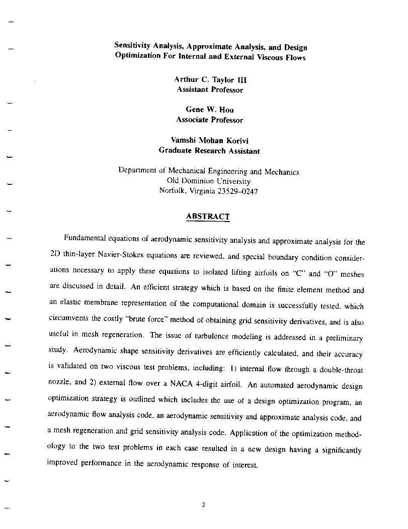
ABSTRACT

Fundamental equations of aerodynamic sensitivity analysis and approximate analysis for the

2D thin-layer Navier-Stokes equations are reviewed, and special boundary condition consider-

ations necessary to apply these equations to isolated lifting airfoils on "C" and "O" meshes

are discussed in detail. An efficient strategy which is based on the finite element method and

an elastic membrane representation of the computational domain is successfully tested, which

circumvents the costly "brute force" method of obtaining grid sensitivity derivatives, and is also

useful in mesh regeneration. The issue of turbulence modeling is addressed in a preliminary

study. Aerodynamic shape sensitivity derivatives are efficiently calculated, and their accuracy

is validated on two viscous test problems, including: 1) internal flow through a double-throat

nozzle, and 2) external flow over a NACA 4-digit airfoil. An automated aerodynamic design

optimization strategy is outlined which includes the use of a design optimization program, an

aerodynamic flow analysis code, an aerodynamic sensitivity and approximate analysis code, and

a mesh regeneration and grid sensitivity analysis code. Application of the optimization method-

ology to the two test problems in each case resulted in a new design having a significantly

improved performance in the aerodynamic response of interest.

2

1.0 Introduction

The focus of the present study is the continued development of efficient techniques for

computing aerodynamic sensitivity derivatives for steady, viscous internal and external flows

(Ref. [1]). In particular, this present work involves a direct extension of the recently developed

methods of Reg. [2] through [7], which have been successfully demonstrated on inviscid and

viscous internal channel flows, to the classic external flow problem of an isolated airfoil. This

extension to external flows is in essence a boundary condition problem.

Sensitivity derivatives are defined as the derivatives of the system responses of interest

(e.g., the specific thrust (Fs) of a nozzle, or the lift (CL), drag (CD), and pitching moment

(CM) coefficients of an airfoil) taken with respect to the design variables of interest (e.g., the

parameters which define the geometric shape of the system, such as the thickness and camber of

an airfoil). Once computed, these sensitivity derivatives are potentially useful in many ways. For

example, the sensitivity derivatives can be used in approximate analysis, where if the changes

in the design variables are small, resulting changes in a system's response(s) can be accurately

estimated, resulting in significant savings in computational costs. In addition, one of the most

important applications of sensitivity derivatives is in engineering design optimization. The use of

sensitivity derivatives in aerodynamic design optimization is demonstrated in the test problems

to be presented.

The present study is therefore design oriented, with the ultimate goal of the work being

the development of tools which can be used by design engineers together with modern CFD

(Computational Fluid Dynamics) software in improving the aerodynamic performance of the

systems to which these codes are applied. Recent research efforts in the subject of aerodynamic

sensitivity analysis with applications to design optimization have been intensive, and Refs. [8]

through [20] is a representative (but not exhaustive) list of closely related works by other

researchers, given here to provide additional background material on the subject, and its status.

The remainder of the work is organized as follows: After the introduction, the next section is

a presentation of theory, a section which is further sub-divided into six sub-sections, including 1)

3

governingequations,2) spatialdiscretizationandimplicit formulation,3) fundamentalequations

of sensitivityanalysisand approximateanalysis,4) boundaryconditions,5) grid sensitivity, and

6) ancillary sensitivity relationships. In the next section, the computational results are given in

application to two test problems, including an internal flow through a double-throat nozzle, and

an external flow over a NACA 4-digit airfoil. The final major section is a summary of the work

where conclusions are given.

2.0 Presentation of Theory

2.1 Governing Equations

as:

where:

The governing equations in this study are the 2-D thin-layer Navier-Stokes equations, given

1 0q

J 0t = R(Q) (1)

OF(Q) OGIQ) 0¢$_(Q)R(Q) - + (2)

0_ 0q 07

Q = [p, pu, pv, peo] T (3)

R(Q) is called the residual, and is clearly equal to zero for a steady-state solution. Q is a vector

of conserved variables, p is density, u and v are velocity components in Cartesian coordinates,

and eo is total energy (i.e., eo=e + _, where e is the specific internal energy of the fluid).

The inviscid flux vectors, F(Q)and (_(Q) are given by:

F(Q) = -_F(Q) + _G(Q)

G(Q) = _F(Q)+ _G(Q)

(4)

4

A transformation to generalized (_, q) coordinates from Cartesian (x,y) coordinates has been

made in Eq. (1), where (x, _y. q,_. qy are metric terms, and J is the determinant of the Jacobian

matrix of this transformation. The Cartesian flux vectors F(Q) and G(Q) are given by:

F(Q) = [/gu./gu-'+ p. pu,.. (peo+ P)u] r

G(Q) = [/gv.puv, pv-'+ p. (/geo+ P)v]r(5)

The pressure, P, is evaluated using the ideal gas law:

P = (?, - 1) /geo -- /9(6)

and -_ is the ratio of specific heats, taken to be 1.4. The thin-layer viscous terms in generalized

coordinates are given by:

(7)

where:g_'l = 0

gv2 -'- O1Ur/ '1- 03Vq

gv3 = Ot3Uq @ Ot2V O

1 1

_v, = ,5o1(u-'). + =,o_(,,._),04

+.3(uv), + Pr('r- t)(_)0

_ = + 5_:3J}' a..,=

q×qY a4 -a3 = j , j

(8)

The molecular viscosity is given by _u, Stokes' hypothesis for the bulk viscosity (A =

-2#/3) has been used, a is the speed of sound, Pr is the Prandtl number (taken to be 0.72),

and ReL is the Reynolds number. Nondimensionalization of Eq. (1) is with respect to p_

and U_, the freestream density and velocity, respectively. The physical coordinates (x,y) are

nondimensionalized by a reference length, L, and the viscosity is nondimensionalized by _u_, the

molecularviscosityof thefreest.ream.Thenondimensionalmolecularviscositycanbecomputed

usingSutherland'slaw andareferencetemperature,T_, the static temperature of the freestream.

For additional simplicity, however, in the laminar flow calculations of this work, the molecular

viscosity is taken to be constant, equal to that of the freestream. For turbulent flow calculations.

the algebraic turbulence model of Baldwin and Lomax [21] is used.

2.2 Spatial Discretization and Implicit Formulation

The governing equations are solved in their alternative integral conservation law form using

an upwind cell-centered finite volume formulation. Only an overview of this method is presented

here, with additional details found in Refs. [22] through [28]. With this approach, the residual

at each cell becomes a balance of inviscid and viscous fluxes across cell interfaces. As an

example, this flux balance for the jk _ cell in a typical computational grid is given by Eq. (9),

for a steady-state solution, and for A_ = At/ = 1

-RJ k = l;'j+½ - 17j-_-_+ (_k+_- -- (_k-½ _ G.,,k+_.'tl+ Gtl__. : 0 (9)

1where subscripts j,k in Eq. (9) refer to the _,q directions, respectively, and subscripts j +

refer to the ( = constant cell interfaces of the jk th cell, subscripts k + t refer to the q =

constant cell interfaces of the jk th cell. (All references to quantities which are evaluated at

the cell interlaces will therefore require only a single subscript, either j + _. or k + ½.) Rjk is the

discrete representation of the residual at the jk th cell. Upwind evaluation of the inviscid fluxes is

accomplished by upwind interpolation of the field variables, Q, from the approximate cell centers

to the cell interfaces, where the flux vector splitting procedure of van Leer [29] is employed. A

third-order accurate upwind biased inviscid flux balance is used in the streamwise (() and in the

normal (q) directions. The finite volume equivalent of second-order accurate central differences

is used for the viscous terms. The resulting discrete higher-order accurate algebraic approximate

representation of the residual at each cell depends locally on cell-centered values of the vector

Q at nine cells. That is, for the jk tla interior cell

Rjk(Q) : Rjk(Qj,k, Qj,k-l, Qi k+I, Qj,k-2, Qj,k+2, Qj-l,k, Qj+l,k, Qj-2,k, Qj+2,k)

(I0)

6

Clearly adjustments are needed to Eq. (10) for interior cell equations which are adjacent to

the boundaries. When written for each cell (including boundary condition relationships to be

discussed) and assembled globally, this can be expressed as

= (o} (ll)

where {Q'} is called the "root" (i.e., the steady-state value of the field variables). Therefore,

Eq. (11) represents a large coupled system of nonlinear algebraic equations, and thus finding

a steady-state solution to the governing equations has been replaced (approximately) by the

problem of finding the root, {Q* }, of this set of algebraic equations.

The governing equations are discretized in time using the Euler implicit method, followed

by a Taylor's series linearization of the discrete equations about the known time level. This

results in a large system of linear equations at each time step, given as

(12)

{Qn+l} = {Q_} + {_AQ}

n = 1,2,3,...

(13)

Equations (12) and (13) represent the fundamental implicit formulation tbr integrating the

governing equations in time to steady-state. In these equations, n is the time iteration index, and

{,n'_Q} is the incremental change in the field variables between the known (n m) and the next

(n+l th) time levels. The matrix, []_-7], is diagonal, and contains the time term.

In constructing exactly the true global Jacobian matrix, [-_], of Eq. (12), both the

interior cell equations as well as the boundary conditions must be considered, (although the

contributions to this matrix from the boundary condition equations are typically neglected in

many CFD codes). Considering the contribution to this Jacobian matrix from interior cell

7

equationsonly, the tour componentvector equationwhich is associatedwith the jk th interior

cell is isolated and extracted from the global linear system. Eq. (12), and is written below as

nz_ n I1[A]{ Qj.k-l) +[B]{nz_Qj.k} +[C]{a_Qj,k+l} +[I)]{ AQj,k_2} +[E]{ _Qj.k+._}+

[F]{n/X, Qj-t.k} + [G]{n/'xQj+l,k} + [H]{ttAQj-2,k} + [[]{ttAQj+2,k} = {Rjak(Q)} {14)

( "1

where _ R_k(Q) _ is given by Eq. (10), and of course Eq. (14)represents the linearized form

of Eq. (10). The nine-point "difference stencil" represented by Eq. (14) is illustrated in Fig.

(1), for a typical interior cell. The nine 4x4 coefficient matrices [A] through [I] of Eq. (14)

are constructed of linear combination of the inviscid and viscous flux Jacobian matrices, and

[B] also includes the time term.

As a consequence of Eq. (14), following global assembly of all interior cell equations, the

resulting global coefficient matrix of Eq. (12) is sparse and has a banded structure, with nine non-

zero diagonals, the individual elements of which are 4x4 block matrices. This matrix structure is

illustrated in Fig. (2), which was taken from Ref. [30]. Note that consistent implicit treatment

of the boundary condition equations and inclusion of these terms in the global coefficient matrix

will sometimes severely disrupt the matrix structure which is illustrated in Fig. (2), depending of

course on the type of boundary conditions. In addition to its use in Eq. (12) for time integration

of the governing equations, this important Jacobian matrix, [_], plays another central role

in this study, which will be shown later.

In principle, Eq. (12) can be repeatedly solved directly (using Eq. (13) to update the field

variables), as the solution is advanced in time to steady-state, and for very large time steps, the

direct method represents Newton's root finding procedure for nonlinear equations [31,32,33].

The direct method however is not necessarily the most efficient procedure with respect to overall

CPU time, and the large storage requirements of the method make its use not feasible in 3D.

Therefore, more commonly, an iterative algorithm is selected for use in the repeated solution

of Eq. (12). Popular choices of these iterative algorithms include approximate factorization

(AF) [34], conventional relaxation algorithms [26,27,35], the strongly implicit procedure (SIP)

8

[36], and the preconditionedconjugategradientmethod[37,38], to namea few. In the present

research,theAF algorithmis usedin the testproblemsto obtainsteady-statenumericalsolutions

to the governingequations.

2.3 Fundamental Equations For Approximate Analysis and Sensitivity Analysis

In this section, fundamental equations of aerodynamic sensitivity analysis and approximate

analysis are reviewed, with additional details given in Refs. [1] through [7]. Consider the

vector, 3. the elements of which are independent variables which are typically called the design

variables. Some, none, or all of the variables may be related to the geometric shape of the flow

problem of interest, although the emphasis of the present study will be that of geometric shape

variation. Computationally, the geometric shape of the domain is defined by the mesh upon

which calculations are made, and the complete vector of (x,y) coordinates which defines the

mesh is represented here symbolically as {X}. For a steady-state solution, the discrete residual

vector given by Eq. (11) is rewritten in the following tbrm

{R(Q*(3),X(3),3)} = {0} (15)

where in the above, the direct dependence of the residual on the computational mesh, {,_ }, as

well as its direct dependence (if any) on the vector d is now emphasized explicitly. Direct

differentiation of Eq. (15) with respect to 3k, the k t_ element of 3, yields

_k } : [_]{0,_kJ + {_} (16)

Term 1 Term "2 Term 3

Equation (16) is an exact derivative of the discrete algebraic residual vector, and represents

the central and most general relationship upon which those which follow in this section are

I_--_], of Term 1 of Eq. (16)is identical to that found in thebased. The Jacobian matrix,

fundamental implicit formulation for time integration (Eq. (12)), and is evaluated here at the

steady-state solution. It is thus well understood. The solution vector, { _"}, is the sensitivity

of the complete vector of field variables with respect to the k aa design variable. The matrix.

9

5_ ' of Term 2 is the Jacobian of the steady-state discrete residual vector with derivatives taken

with respect to the complete vector of (x,y) grid coordinates, and is documented in Refs. [3,5].

{ax /The vector, _ j,, of Term 2 contains what is known here as the grid sensitivity terms, and

is discussed in greater detail in Ref. [4], and also will be given special consideration later in

{oR } (Term 3)accounts for derivatives resultine from directthe present study. The vector, _ ,

dependencies (if any) of the residual vector on 3k.

In the event that 3 k is no_.._ta geometric shape related design parameter (e.g.. the back pressure

in a subsonic nozzle, or the angle of attack (a) or freestream Mach number (*l_)/'or a airfoil)

then Term 2 of Eq. (16) will be zero. If 3k is a geometric shape design parameter, its entire effect

on the residual will typically be felt through the grid, and Term 3 of Eq. (16) will generally

be zero. Therefore, Eq. 16) becomes

when variation of geomemc shape is not involved, and becomes

when 3 k is a geometric shape design parameter. Eq. (18) represents the central relationship

which is successfully demonstrated in Ref. [4] for accurately computing aerodynamic sensitivity

derivatives with respect to variation of geometric shape.

An approximate version of Eq. (18) which is useful in approximate analysis for estimating

the steady-state solution changes which occur in response to small but finite geometric shape

variations is given by

[oRj (19)

where the approach represented by Eq. (19) is studied in detail in Refs. [3] and [5] for internal

inviscid and viscous flows, respectively. In developing approximate analysis methods, other

approaches of interest which might be used are

1o

for variationsother thangeometricshape,(which is anapproximateversionof Eq. (17)), aad

(21)-

for geometric shape variations only (which is a minor variation of Eq. (19)).

a typical design sensitivity analysis, the solution vector, { _ }, of the preceding equationsIn

will provide far more information than is actually sought, and only a relatively small subset of

this vector is extracted for use. For example, if the sensitivity derivatives of the aerodynamic

forces on a solid surface boundary are to be calculated for a viscous flow. then the sensitivity

derivatives of the surface pressures and velocity gradients at the wall will be needed, which can

{ °---qL} This is explained more fully in a subsequent sub-section,be obtained as a subset of J,3_ '

where the ancillary sensitivity equations of specific use herein are presented.

2.4 Boundary Conditions

In the implementation of the fundamental equations of aerodynamic sensitivity analysis and

approximate analysis, which were reviewed in the previous sub-section (Eqs. (15) through (21)),

the consistent treatment and inclusion of the boundary conditions in these equations is essential,

and must not be considered optional, as it typically is in the integration of the equations in

time (Eq. (12)). The severely erroneous results which can arise as a consequence of failure to

properly treat the boundary conditions are illustrated in an example problem in Ref. [2], with

additional documentation on boundary condition treatment given in Ref. [6].

For the isolated lifting airfoil problem, where the governing equations are typically solved

on "C" or "O" meshes, the consistent treatment of the boundary conditions (during sensitivity

analysis) is considerably more involved than that which is typically encountered in handling

the boundary conditions for standard internal flow problems. Therefore, the objective of this

section is to describe these difficulties, and to discuss various remedies. Many of the ideas to

be presented in this section are taken from Refs. [33,39] involving the use of Newton (direct)

solvers in obtaining inviscid and viscous steady-state solutions to airfoil problems.

11

-.g

2.4.1 Airfoil Surface Boundary Conditions

The consistent treatment of the boundary conditions which are applied on the surface of the

airfoil in this study (i.e., standard no-slip conditions) does not present any additional difficulty

beyond that which is encountered for the boundary conditions which are used in typical internal

flow problems. That is. the explicit application of the airfoil surface boundary conditions (as

well as the application of all boundary conditions which are used in the internal flow problem to

be presented) can be represented at each point where the boundary conditions are applied (i.e..

at the boundary cell faces in the present study) as the solution of a boundary condition residual

equation of the form given by

{RB(Q;(_)),Q_'(_J),Xt(3),,))} = {0} (22)

where {RB } is a nonlinear four component vector function of (at most) the local field variables,

Q_, at the boundary cell face. Q_, the local field variables at the first interior cell adjacent to the

boundary, XI, the local coordinates of the grid, and also the very likely possibility of an explicit

dependence on .) is included. Differentiation with respect to tit, the k th design variable, yields

-L0--_BJ [ 03k - [-EQ-_JI, 03k = [ _ (23)

when geometric shape is not involved, and

[oR.l OQ; [o °l ox,;0--_BJ[03k}-- } = { (24)L_ LSgTjLOQIJ

when geometric shape variables are involved. For approximate analysis, Eq. (23) can be written

as

[0R ] [OR.] .- [O--_BJ{_Q;} - k-g-_[j {_Q_} _ {0RB}a3k_ (25)

if geometric shape is not involved, and Eq. (24) can be written as either of the following two

equations

[ORB] [OR_] [ORB]--[0--_B] {AQ;} - [0Qtj{cXQ[} _ L-b-_l {.xX_} (26)

1 1 . [OR.l{Ox-[0--_BJ {AQ_}- [-_i]{ QI}_ [0---_[ ] _?;:__3 k(27)

12

.,_,..

for predictions of geometric shape change.

Equations (23), (24), (25), (26), and (27) are of course fully a part of the global linear

systems of equations given by Eqs. (17), (18), (20), (19) and (21), respectively, and can be

explicitly included and solved simultaneously with the interior cell equations during the solution

of these linear systems. Alternatively, yet equivalently, these boundary conditions equations can

be pre-eliminated (i.e., pre-solved and substituted into the remaining interior cell equations) prior

to simultaneous solution of the global linear systems. Pre-elimination of the boundary condition

equations is the approach selected in the present study, and is explained in greater detail in Ref.

[21. Note that in general, contributions to the Jacobian matrix. [_], of the fight-hand sides of

Eqs. (16), (18), (19) and (21) can also occur (for some boundary condition types) from these

condition equations(in addition of course to the contributions to the matrix, [-_-_] ).boundary

It is significant to note that simple boundary conditions of the form given by Eq. (22) result

in consistently linearized boundary condition equations (i.e., Eqs. (23) through (27)) which, when

included, do not in any way alter the basic structure of the coefficient matrix I02-_], illustrated in

Fig. (2) (i.e., the nine-diagonal, 4x4 block structure is preserved exactly), and thus direct solution

of the fundamental systems of equations of sensitivity analysis and approximate analysis is not

further complicated by inclusion of these boundary conditions equations. Unfortunately however,

this is not the case in general, for all boundary condition types, as will be seen subsequently.

2.4.2 Periodic Boundary Conditions For "C" and "O" Meshes

When calculating flows over airfoils, in the likely event that a "C" or "O" type mesh has

been selected for the calculations, "periodic" boundary conditions are applied along the "wake

cut" of the computational grid. There are different ways that these periodic boundary conditions

could be applied. In the present research, the explicit application of these boundary conditions

is not expressed (as before) as the solution of special boundary condition equations of the type

given by Eq. (22). Instead, interior cell residual equations for the interior cells immediately

adjacent to the "periodic" boundaries (i.e., the wake-cut) are each expressed as functions of

cell-centered values of the vector Q at nine cells in the domain (i.e., for a higher-order accurate

13

%,

upwind spatial discretization), where this functional relationship in physical space is identical

to that expressed by Eq. (10) tbr a general interior cell. This means that wherever necessary.

the evaluation of the inviscid flux vectors of Eq. (9) is accomplished by a consistent upwind

interpolation of the field variables from local interior cells across the wake cut, and that the terms

of the viscous flux vectors are evaluated using consistent central differences across the wake cut.

Although the functional relationship expressed by Eq. (10) for a general interior cell equation

is preserved in physical space for interior cells involving periodic boundary conditions, clearly

it is no_._!tpreserved for these cells (with respect to the structure and ordering of the cells) in

the computational domain. That is, when periodicity is involved, the interior cell equations

depend explicitly on the field variables at local neighboring cells in the computational grid, and

in addition, become functionally dependent on the field variables of cells which are quite distant

in the computational ordering. Consequently, the linearized version of Eq. (10), given by Eq.

(14) for a general interior cell, must be modified for interior cells involving periodicity, in order

to properly account for these boundary conditions. Periodic boundary conditions affect each first

and second interior cell equation immediately adjacent to the boundary where "periodicity" is

enforced, resulting (for the higher-order spatial discretization) in two periodic 4x4 matrix terms

contributing to the left-hand side of Eq. (14) for the first interior cell equation, and one such

periodic term for the second interior cell equation.

The most significant impact of the periodic boundary conditions is that there is some

IaFt] neat, nine-diagonal structurerestructuring of the coefficient matrix, _ , where the banded,

which is illustrated in Fig. (2) is no longer preserved exactly. This is illustrated in Ref. [33],

and is of course is a consequence of the previously discussed adjustments to Eq. (14) which

are required for the interior cell equations involving periodicity. Furthermore, depending on the

direction which is selected when ordering sequentially the individual cell equations for assembly

into the global linear system (either the tangential (J) to the airfoil direction, or the normal

(K) to the airfoil direction), the non-zero contributions to the global coefficient matrix from

the periodic boundary conditions will fall either inside or outside of the central bandwidth of

the matrix. (Note: The central bandwidth here refers to all of the matrix elements, either zero

14

or non-zero,which fall betweenthe outermostdiagonals,[HI and [I], of Fig. (2) and is thus

the bandwidthof the matrix, neglectingperiodic terms,if any,which fall outside.) For "C" or

"'O" meshcalculations,if theequationsarenumberedin the tangential(J) direction, theperiodic

coefficientswill all fall insidethecentralbandwidth,butwill all fall outsidethecentralbandwidth

(someat extremedistances)if the numberingis in thenormal (K) direction. (Exception:There

existsa specialmethodexplainedin Ref. [33] for numberingtheequationsin the"'K'" direction

for "'C'" mesheswheretheperiodiccoefficientsall fall completelyinside thecentral bandwidth.

This methodresults in a doubling of the central bandwidthof that which is achievedwith a

standard"'K" ordering of the equations,and hencethis non-standardordering was rejectedin

the presentstudy).

A "J" directionorderingof theequationswill thereforein principleallow the useof a pure

bandedmatrix direct solver solutionprocedurewhich takesadvantageof the fact (in termsof

storageand work) that outsideof thecentralbandwidth,all of thematrix elementsarezero. In

contrast,for a pure direct solutionof the linear system,a standard"K" direction orderingwill

require the useof a full matrix solver to accountfor the periodic terms,which is not feasible

for practical fluids problemsinvolving the full governingequations,even in 2D.

For typical airfoil calculations,the "J" dimensionof the grid is usually significantly larger

than the "K" dimension. A standard"K" ordering of the equationswill thus result in a

significantly smaller central bandwidthof the coefficientmatrix than will a "'J" ordering. To

overcomethisdilemma,a hybriddirect solver/ conventional Richardson type relaxation strategy

is proposed and implemented in the present study, for airfoil problems on "C" and "O" meshes,

as follows:

1) A "K" direction (i.e., normal to the airfoil) numbering of the equations is used in

constructing the coefficient matrix, [_-_], in order to minimize the width of the central

bandwidth.

2) The coefficient matrix is split into two parts, such that

[ 0_._] [M] + [N] (28)

15

3)

where the matrix [M] containsall of the elementswhich fall inside of the central

bandwidth of I_l" Thus [M] has the matrix structure illustrated in Fig. (2). The_ J

FoR]matrix [N] is thus very sparse, and contains all of the non-zero contributions to l_j

which fall outside the central bandwidth, resulting from the periodic boundary conditions.

The matrix [M] is LU factored directly using a conventional banded matrix solver, to

yield

[M] = ILl[U] (29)

4) A conventional Richardson type iterative strategy is invoked which in principle could

be applied to Eqs. (16), (17), (18), (19), (20), and/or (21). For example, if Eq. (18) is

selected, the iterative strategy is

[L][U]{0Q*_ i [OR] 0_( _ _'0Q*; L-1

i = 1,2,3.. •., (imax) k (30)

k = l, ndv

where in the above, 'i' is the innermost index, (imax) k is the maximum number of iterations

required to converge the k th linear system to the desired tolerance, 'k' is the outermost index,

(imax) k

which associates the solution vector, {0_} with a particular k th design variable, and

ndv is the total number of design variables for which sensitivity derivatives are required. It is

emphasized that since [L] and [U] (in addition to 5"g and [N]) are constant with respect to

the indices 'i' and 'k', they only need be computed once and repeatedly reused. Following the

LU factorization, a single iteration of Eq. (30) is inexpensive, of course, since [L] and [UI are

lower and upper triangular matrices, respectively.

The coefficient matrix, [_-_}, is diagonally dominant for a first order upwind spatial

discretization, but is not diagonally dominant for a higher-order spatial discretization [26], and

therefore, convergence of the iterative strategy represented by Eqs. (28), (29) and (30) is not

16

assured [35]. In the airfoil test problem to be presented, the iterative strategy of Eq. (30) was

at first divergent, but was subsequently made convergent through the simple use of a single

conventional under-relaxation parameter. ,.,: (omega). Other remedies which are suggested as

possible methods to correct the failure of this iterative strategy to converge include, but are not

limited to:

1) Use of a first order accurate upwind spatial discretization for the inviscid terms of the

first row of interior cells immediately adjacent to the wake cut. which will result in

only a single non-zero periodic 4x4 matrix coefficient contribution (instead of three such

coefficients) to the matrix [N] of Eqs. (28) and (30), for each point where periodicity

is enforced.

2) Use of a "'ghost" cell equation at each point where periodicity is enforced, which is

retained explicitly in the global coefficient matrix, resulting in a more strongly implicit

treatment of the periodic terms, with complete preservation of higher-order accuracy

across the wake cut. This is the approach of Ref. [33], where difficulties with

convergence of the iterative strategy were not encountered [39].

3) Use of matrix pry-conditioning.

In addition to the contributions to the matrix, I_r_], resulting from the application of periodick. -- ,.I

conditions, there are also contributions to the matrix, I_-_/_}, of Eqs. (16), (18), (19,,boundary

and (21), which must be considered for viscous flow. For inviscid flow, there are no additional

needed to [_1 to account for periodicity. However, a consistent treatment of alladjustments

viscous metric terms in the application of periodic boundary conditions will result in the need

for some adjustments to some of the terms of _ to properly account for the periodicity. A

close examination of the documentation given in Ref. [5] on the details of the construction of

the viscous terms of I.-_RX]will provide additional explanation and verification of this.

17

2.4.3 Far.Field Boundary Conditions

The far-field boundary conditions which are used in this study make use of the Riemann

invariants, and these boundary conditions are given in Refs. [331 and [401. For lifting airfoils, it is

well known that significantly improved computational accuracy can be achieved with the addition

of a "'point-vortex" correction to these boundary conditions. This "'point-vortex'" correction is

developed and presented in detail in Ref. [40], and will be addressed in the context of its treatment

in sensitivity analysis in this sub-section. If this point-vortex correction is no__Atincluded, then the

explicit application of the far-field boundary conditions at each location can be expressed exactly

as the solution of a boundary condition residual expression of the form given previously by Eq.

(22). In this event, the contribution from the far-field boundary conditions to the equations of

sensitivity analysis and approximate analysis (i.e., to Eqs. (16) through (21)) is therefore very

straightforward, using Eqs. (23) through (27).

The use of the "point-vortex" correction described in Ref. [40] to improve the far-

field boundary conditions is straightforward to implement in an explicit sense. Its explicit

implementation involves the use of a point-vortex (centered at the quarter chord) representation

of the airfoil, where the strength of the point-vortex (i.e.. the circulation, F) is proportional to

the lilt coefficient, CL, of the airfoil. The purpose of this point-vortex is to more accurately

model the influence of the lifting airfoil on the velocity field in the vicinity of the far-field

boundaries, (compared to the alternative of assuming a freestream velocity field here), resulting

in more accurate airfoil calculations, particularly as the extent of the far-field boundary from

the airfoil is decreased.

The implementation of this point-vortex correction results in a numerical coupling between

the far-field boundary condition equations and (through the lift coefficient, CL) the field variables

(and also the x,y grid coordinates) on and immediately adjacent to the surface of the airfoil. As

a consequence of this coupling, there are algebraically messy, complex additions to the global

Jacobian matrix, I_r_ 1 (which destroy the banded matrix structure, illustrated in (Fig. (2))and

[o.]also to _ . In order to avoid the task of explicitly deriving these terms and their precise

18

locationsin theseglobalJacobianmatrices,a simplifying strategyis proposed,which makesuse

of the following ideas:

1. In the discretesystemof algebraicequationswhich models thesteady-statefluid flow

(i.e., Eq. (11)), the lift coefficient,CL, is to be treatedasanadditional field variable.

2. The chain rule is employedjudiciously.

. In a typical sensitivity analysis for airfoil design, the sensitivity of the lift coefficient

with respect to the design variables will be sought. Explicit expressions are therefore

available for use in calculating the sensitivity derivatives of CL with respect to the design

variables, following solution of the global sensitivity equations. (This expression for CL

is given in a subsequent sub-section).

. Recall that a strategy which involves iteration will be used to solve the equations of

sensitivity and approximate analysis to account for the periodic boundary conditions

(regardless of whether the point-vortex correction is used or not).

When the point-vortex correction is included, the boundary condition residual equation which is

solved at each far-field boundary cell face can be expressed in a form similar to that of Eq. (22),

except that an explicit dependence of the boundary condition equation on CL is now identified.

That is, Eq. (22) becomes:

eL)} = {0} (31)

where all the terms of Eq. (31) are as previously defined. Differentiation with respect to 3k,

and applying the chain rule on the term involving CL, the result is

ORB] 0 * ORB] 0Q r; [0RB] OX, act.- O-O-ffB] { _3kB } - [ { _J = [_t ] {}+{0RB;_ _J + I. 0RB;0cLJ-_k (32)5- i J

The four component vector, _ , is very straightforward to derive analytically, since the

explicit dependence of RB on CL is known and uncomplicated [401. There are also additions

to the matrix, [o__] , which are straightforward to derive, which arise as a consequence of thisL u.x/ j

19

condition correction. The scalar term, _, is evaluated using an expression of theboundary

form

d3 k - OQ ] _ + [ /-)X 03k J + 03-----k (33)

where the global column vectors, and ax j' are sparse. Since the value of a(_ is

likely to be at least one of the desired final results of an airfoil sensitivity analysis, the precise

terms involved in Eq. (33) (i.e., {_}T and ,/a--ga-c}T)0x have been derived analytically for this

purpose, and are given in a subsequent sub-section. Note in Eq. (33) that the notation for a total

derivative has been used on the left-hand side of the equation, indicating that the tota....._lrate of

change is included in the expression, and thus distinguishing it from the partial derivative (which

accounts for explicit dependencies of CL on 3k, if any) on the right-hand side of the equation.

It should be understood, however, that _ is still a partial derivative in the sense that CL is in

general a function of multiple independent design variables.

Specialization of Eq. (32) to the case of either geometric or non-geometric shape design

variables and to the case of either sensitivity analysis or approximate analysis is analogous to

that shown in Eqs. (23) through (27). In particular, for approximate analysis, the term _ of

Eq. (32) becomes ACL, and Eq. (33) becomes:

ACE _ 0Q J {AQ*}+ [ 0X J {AX} +_A3k (34)

At this-point, the far-field boundary condition equations given by Eqs. (32) and (33) are in a

convenient form for assembly into the global system of equations for subsequent solution in

the hybrid direct solver / iterative strategy previously described, where iteration is also used to

account for the periodic boundary condition terms (whether or not the point-vortex correction

is included). Global assembly of Eq. (32) into the iterative strategy of Eq. (30) results in the

following modified iteration strategy to account for the point-vortex correction

[L][U]fOQ, i 0X . , i-1-ff_-k} = [_]{_}-[N]{_} + {_} dCci-ldjk/

i = 1,2,3, • • -.(imax) k (35)

k = 1, ndv

20

{oR}where in Eq. (35) the only non-zero contributions to the global vector, _ , are from the

far-field point-vortex corrected boundary condition equations. The scalar term is repeatedly

calculated for all T and "k' indices using the expression

(36)

The iterative strategy of Eq. (35) thus avoids the need for determining explicitly the algebraically

messy contributions of the point-vortex corrected boundary conditions to the Jacobian matrices.

oR!_7-_j and Lo.x j .

2.5 Mesh Sensitivity Analysis

In this section, calculation of the terms of the mesh sensitivity vector, { '_k }' of Eqs. (t6),

(18), and (21) is given special consideration. One approach which can be used for calculation

of these terms is the "brute force" finite difference method, where the geometric shape design

parameters are perturbed slightly, one at a time, and the mesh generation program (which was

used to generate the initial mesh) is repeatedly re-run to generate perturbed grids. Then, each

grid sensitivity vector is calculated as

{ 0,'_ } {'f((,3k+_3k)}--{X(3k--_3k)}_k _ (37)2A3k

where in the above, central finite difference approximations are used for greater accuracy, but

require the generation of two perturbed meshes per design variable instead of the one which

is required using a forward finite difference. The principle advantage of this approach is that

it is conceptually simple and easily applied. For this reason, it is also well suited for use

in an automated design optimization loop. Since by design the equations of mesh generation

are typically very smooth, the method can be expected to be reliable in producing satisfactory

accuracy. Furthermore, for simple 2D geometries using algebraic grid generation, the procedure

should be computationally efficient, even when the number of design variables is large.

High quality elliptic and hyperbolic grid generation codes, which are often selected for

generating "C" and "O" airfoil meshes, are tar more computationally expensive to use than are

21

their algebraic counterparts, and thus use of the "brute force" method to obtain grid sensitivities

in this case could become excessively costly, particularly if the number of design variables is

large, and if the computations are to be made repeatedly in an automated design loop. One

strategy proposed in Ref. [41 to help restore computational efficiency to this problem would be

to differentiate analytically the equations of mesh generation (for the particular mesh generation

code of choice), to determine the Jacobian matrix of the entire grid, J_, with respect to the grid

points on the boundary of the domain, i_. Then grid sensitivity derivatives could be efficiently

O.k

calculated using the relationship

(38)

Other researchers [41] have implemented the approach of Eq. (38) in application to the airfoil

grid generation program of Ref. [42]. Another important consideration with respect to some

sophisticated grid generation codes is that they are used interactively, which would prohibit their

use (interactively) in an automated design loop.

In order to help overcome these difficulties which have been discussed, a procedure is

proposed herein for use in the repeated evaluation of grid sensitivity terms, as well as for use

in efficient grid regeneration. The method, which will be presented subsequently, is based

on an "elastic membrane" analogy to represent the computational domain, and grid sensitivity

derivatives are calculated from a standard structural analysis computer program using the finite

element method.

As the geometric shape of the flow domain is continuously changed, as required by any

geometric shape optimization process, the mesh points in the domain must be properly adjusted

in the design iterations, to avoid ttae numerical errors induced by excessive mesh distortion.

The requirement of mesh regridding distinguishes shape design optimization from other design

optimization applications. A simple way for automatic mesh regridding can be established by

introducing a set of basic displacement vectors, 9'k, to describe the patterns by which the mesh

is regridded. The relationship between the original mesh, ;Ko, and the regridded one, X, can

22

thenbeexpressedin the form of a linearcombinationof thesebasicdisplacementvectors,and

their associatedweighting coefficients,3 k, as

ndv

X -=- Xo q'- _ ::]k_"k (39)k=l

where in the above, ndv is the number of design variables, if the weighting coefficients are taken

to be the design variables. The vector, Xo, represents the initial mesh, which is produced using

any conventional mesh generation code of choice. In this case, the basic displacement vector,

9> is simply equal to the required mesh sensitivity vector, {_ }, of Eqs.(16), (18), and (21 ).

That is, the grid sensitivity derivatives are calculated by differentiation of Eq. (39), which yields

03 kj = {%'k} (40)

Note that the grid sensitivity vectors, {_k }, do not change when the design variables are changed,

provided that the domain is always regridded using Eq. (39), as the shape of the domain changes.

Therefore, these grid sensitivity derivatives need only be calculated once and then stored prior

to the start of an aerodynamic optimization strategy, and they can be repeatedly re-used as often

as needed for grid sensitivity analysis, as well as for automatic mesh regeneration.

The basic displacement vectors, 'qk, can be in any form; however, they must be independent

of each other. In structural shape design optimization, the elastic displacements induced by the

boundary perturbations are commonly selected to represent the basic displacement vectors. In this

way, the movement of the mesh points is governed by the nature of linear elasticity, which not

only preserves the continuity of the mesh, but also avoids any mesh-overlapping. It is proposed

herein that the same practice can be applied to aerodynamic shape optimization problems, in

which an imaginary elastic medium is introduced to represent the computational domain.

More specifically, the basic displacement vectors can be generated by either the fictitious

load method [43], or the prescribed displacement method [44]. The former produces the basic

displacement vectors by applying a unit load at each of the nodes along the boundary in the

direction along which the node is allowed to move. This concept is illustrated in Fig. (3), for

a representative airfoil grid. The latter, however, produces the basic displacement vectors by

23

imposinga non-zerodisplacement(in responseto a unit changein eachdesignvariable)along

the varied boundary. This conceptis illustrated in Fig. (4), for a representativeairfoil grid.

The fictitious load method is usually applied to the case where the location of each node on the

varied boundary is considered as a design variable, whereas the prescribed displacement method

is good in the case where the shape of the boundary to be designed is parameterized.

In the following, a NACA 4-digit airfoil is employed as an example to demonstrate the

application of the prescribed displacement method for mesh-regridding in an aerodynamic shape

optimization environment. The profile of the NACA 4-digit airfoil can be precisely represented

by polynomials in terms of the maximum thickness, T, the maximum camber. C, and the location

of maximum camber, L, as

f(x)+C(2Lx x_')/L 2,

- x<L(41)

y(x)= f(x)+C(l-2L+2Lx-x2)/(1-L) 2. x>L

where

f(x) = +.ST(0.2969v'_- 0.126x - 0.3516x 2 + 0.2843 x 3 - 0.101.Sx 4) (42)

where, the + in the expression for f(x) is '+' for the upper surface of the airfoil, and '-' for

the lower surface.

Since the derivatives of the airfoil shape with respect to T, C, and L are continuous, it

is understood that small changes in T, C, and L will induce small changes in airfoil shape.

Therefore, according to a Taylor's series expansion, such a change in the airfoil shape can be

expanded approximately into a linear function of ,.kT, ._kC, and AL, given as

0yo(x) 0yo(x) 0yo(x)y(x) = yo(X) + 0_AT + 0----_/_C + 0---L---AL (43)

whereAT = T - To

.XC = C - Co (44)

AL = L - Lo

where To, Co, and Lo are the initial values of these three shape parameters associated with the

initial airfoil shape, yo(X), and the initial grid, Xo.

24

OVo(X) 0Vo(X)The derivatives -%-_, ""FU-, and _ in Eq. (43) represent special patterns which control

the allowable changes in the airfoil's shape. The new mesh, X can be defined in a form given

by' Eq. (39) as

X=Xo+&T.{'z+&C'._.,+&L.V} (45)

where __ST, XC, and XL are taken to be the design variables (or equivalently T, C. and L

are the design variables, through Eq. (44)). The basic displacement vectors, _"l, V2. and V3

can be obtained by the prescribed displacement method, discussed above. These vectors are

obtained numerically through implementation of a finite element model, with each cell in the

computational mesh being considered as a plane stress quadrilateral element. A finite element

matrix equation is formed to solve for each basic displacement vector (i.e., the movements of

all the grid points) which is realized throughout the elastic membrane model of the domain, in

response to the non-zero boundary movement which is specified through Eq. (43), for a unit

change (or some other conveniently scaled change) in each of the design variables. Note that

the finite element matrix equation is linear with a symmetric and banded coefficient matrix,

which is solved directly by a single LU factorization, followed by multiple re-uses of this LU

factorization as multiple solutions (i.e., one solution, _2k, for each design variable) are obtained

for multiple "'load vectors" through simple efficient forward and backward substitutions.

It is clear that Eq. (43) represents a particular parameterization of the surface of the

airfoil which will only closely approximately the NACA 4-digit parameterization defined by

Eqs. (41) and (42) if AT, AC, and AL are small. However, if during design it is not a

requirement to remain exactly within or close to the allowable shapes defined by the NACA

4-digit parameterization, then of course Eq. (43) is a valid (but different) parameterization of

the airfoil shape, even for large AT, AC, and AL. Thus the classic NACA 4-digit airfoil is

presented here only as an example.

In order to demonstrate and validate the mesh regeneration strategy, a numerical example is

given. Starting with an extremely coarse initial grid, Xo, with only 21x10 points (tbr illustration

purposes), for a NACA 1412 airfoil (i.e., To--0.12, Co--0.01, Lo=0.40), generated using the grid

25

generation code of Ref. [42], the domain was regridded using Eq. (45) for a new airfoil shape

defined by Eq. (43) and (44), for C=0.04, T=To, and L=Lo. The initial airfoil and grid is shown

in Fig. (5a), where in Fig. (5b), the new airfoil and grid are shown. The changes which are

seen in the new mesh resulting from the application of this methodology appear satisfactory in

this test example.

2.6 Ancillary Sensitivity. Relationships

The purpose of this sub-section is to include some important extra terms and relationships

which are used in the present study in computing sensitivity derivatives, in order to make the

presentation of the methods more complete. Specifically, expressions are given for generalized

aerodynamic force and moment coefficients in 2D, and their sensitivity derivatives. In addition,

expressions are derived for use in computing the sensitivity derivatives of the thrust, mass flow

rate, and specific thrust of a nozzle.

Fig. (6) illustrates the ida element (oriented at an arbitrary angle in space) which is located

on the boundary of the geometric shape of interest, over / through which the fluid is passing.

In the figure, the coordinates (xb_, Ybi) and (x_+,, Yb_+_) are the physical (x,y) coordinates at

either end of this i_ element, and are assumed to be nondimensionalized by L, the reference

length. The convention is established that as one moves along the surface in the direction of

increasing the index, 'i', then the solid surface is on the right, and the fluid is on the left.

Nondimensional pressure (Cp) and skin friction (Cf) coefficients which are associated with

this i t_ element on the boundary are defined as follows

Cp_ = Pb_ Cfl = %_ (46)_ _,}rl rT2 1,_ it2

where in the above, P_ and "r'b_ are the pressure and shear stress, respectively, which are

associated with the i _ element on the boundary, and ._p_I52_ is the dynamic pressure of the

26

freestream. Nondimensional force coefficients in the x and y directions, given as Cx, and ('y,,

respectively, for the i th surface element, are given as

Cx, _-- ("pi (Ybi+l -- Ybi

C =C-Yi -Pi (Xbi -- Xbi+_

(47)

The total force coefficients in the x and y directions are of course given by summing the above

expressions over the total number of elements of interest, NE, and the result is

NE

C Z('

i=t (48)N'E

('Y = Z Cyi

i=l

Sensitivity derivatives of these force coefficients taken with respect to 3k are given as

dC× L {/')Cpi ,_ I,Ybi+, { OYbi+__k OYbi) }03k= - yu,) + Cp,\dAk ,=1

0,3 k 03 k

(49)

OXb'+t) }d3---7"= Z I. 07k • - Xb,+,) + Cp,\ 03k 03ki=1 ' '

N_ l 6_Cf, (,.hi+ (6_yb,+I _-_Ybi ) }+ " ' -yu,)+ v 04 04L-=-I

Oxb _ etc., are evaluated as being elementsNote in the above expressions that terms such as ,,"b_, oak '

of the vector { _} of the previously discussed right-hand side of Eq. (16), (18), or (21)and

oc0 oc, { }and also _ are obtained from the vector _ by solution of these equations. (Note:

Since C ac,f, involves gradients of the velocity at the ith element of the boundary, then

0 "involves terms from both { _} and { _ }, resulting in an expression not shown here which

is algebraically complex.)

If the sensitivity derivatives of the lift (CL) and drag (CD) coefficients of a body (e.g., an

airfoil) are desired, it is only necessary to convert to a new coordinate system with axes aligned

27

in the L and D directions,which are rotatedat an angleof attack,a, with respect to the x and

y axes. The lift and drag coefficients are then calculated as

('L = ('yCOSO--('-xsinct (5O)

('D = Cy sinct + ('xCOS_ (51)

The corresponding expressions for the sensitivity derivatives of the lift and drag coefficients are

dCL d('y dCx- cos a - _ sin o (52)

d3k d3k d3k

d . D dCy dC×

d3k -- dAk sin a + _ cos c_ (53)

Note Eqs. (64) and (65) are not valid if the angle of attack, o, is the design variable (i.e., if o, -

3k). In this special case, these expressions would simply have additional terms. (See Eq. (33).)

In addition, for airfoil calculations, the sensitivity derivatives of the pitching moment

coefficient, CM, could likely be of interest in a design problem. The moment coefficient. C._t,,

which is associated with the it_ element (see Fig. (6)) on the solid wall boundary of interest,

about the point (Xo, Yo), with the convention that a positive moment is clockwise, is given by

CM, = Cx, (yc, - yo) - Cy,(xc_ - xo) (54)

where the coordinate (xc_, Yci) is the midpoint of the iit' element on the boundary. That is

t t

xci= (xb +l = + yu ) (551

The total moment coefficient is of course the sum of all the elemental moment coefficients over

the total number of elements on the boundary of interest, given by

NE

CM = Z C,M, (56)i=l

28

The sensitivity derivative of the pitching momentcoefficient with respectto the kth design

variable is thus

d3k i= t i=

where

0yu,)0, k -'\ O, k 2\ O,3k+5-2( (58)

In the present study, an internal flow problem was considered where the sensitivity derivatives

of the thrust, T, mass flow rate, vh, and specific thrust, Fs, of a nozzle are of interest, and the

xpressions used in these calculations are developed next. The total thrust which is produced by

a nozzle can be calculated from the previously defined force coefficient, Cx, summed over all

of the interior solid walls, plus an additional term involving the integrated static pressure over

the inflow boundary of the nozzle. That is

NEJ

T = -Cx + Z cpj (yi+l - YJ) (59)

j=l

where in the above, a positive thrust acts in a direction opposite to the positive direction of the

x axis, the y axis is assumed to be in or parallel to the plane of the inflow boundary, Cp, is the

static pressure coefficient of the jth element on the inflow boundary, yj and Yj+l are the starting

and ending coordinates, respectively, of the jth element on the inflow, where the direction of

increasing the index, 'j', and the positive y direction are in this case defined to be always the

same, and NEJ is the total number of elements on the inflow boundary. Nondimensionalization

of T in Eq. (59) above is of course the same as defined previously for Cx. (Note: The expression

above does not consider the aerodynamic forces, if any, due to flow over the exterior surfaces

of the nozzle.) The sensitivity derivative of the thrust is

NEJ NEJ

dL_kdT_ dCxd'3k 0Cpj0,'_k (0yj+l 0yj)+ (YJ+ - yJ)+ Z %j= _ j= _ 03k Oak (60)

29

The mass flow rate, m, through the nozzle can be computed using the expression

NEJ

th = Z PJ LIJ(}'J+I -- YJ)

j=l

and the sensitivity derivatives become

NEJ

(tril (OYj+l Oyj)([,_---7 -= Z pjtlj 03 k ()i_kj--1

:,'EJ Ouj .xEj Op___£. ..+ Z PJo-57(YJ+1- :J) + - :'it

j=l j=l

(6l)

(62)

Often with nozzle calculations, the specific thrust, Fs, is a system response of interest, and is

defined by

TFs = .-':- (63)

m

and the sensitivity derivatives can be calculated using expressions previously defined

dT _ T ,:tindFs rfi _ d3k

d3 k rh 2(64)

3.0 Computational Results

3.1 Internal Flow -- Double-Throat Nozzle Problem

3.1.1 Description of the Test Problem

The first test problem to be presented is that of an internal flow through a double-throat

nozzle, where the flow is accelerated from a Mach number on the inflow boundary of about

0.10, to a Mach number which exceeds 2.80 at some places on the outflow. The Reynolds

number, REL, is 1130, based on a reference length, L, of one-half the height of the nozzle at

the smaller of the two throats. Other researchers have conducted numerical studies on the flow

through this nozzle geometry, with documentation provided in Refs. [5,45,46,47].

30

A computationalgrid is usedwith 171 points evenly spacedin the streamwisedirecuon,

and 38 points with grid stretchingin the normal direction, to resolveviscousgradientsin the

vicinity of solid walls. Fig. (7) illustrates the grid and geometry. Boundaryconditions are

?ecified as tbllows:

1) On the inflow, entropy and stagnation enthalpy are held constant at the freestream values,

the v component of velocity is zero, and the u component is extrapolated from the

interior of the domain.

2) On the outflow boundary, all variables are extrapolated.

3) On the lower wall, velocity no-slip is enforced, and the wall static temperature is specified

to be that of the stagnation temperature of the freestream.

4) On the upper boundary of the computational domain (i.e., along the centerline of the

nozzle), flow symmetry boundary conditions are enforced.

The Mach contours for the steady-state laminar flow solution through the nozzle are shown in

Fig. (8).

The geometry of the nozzle is defined parametrically using analytical expressions which are

presented subsequently, where this material is also given in Ref. [47]. Because of symmetry,

it is only necessary to parameterize either the lower or the upper solid wall surface. The upper

wall is selected here. The wall is described using five polynomial arcs, as illustrated in Fig.

(9). In all cases, continuity of slope is enforced at the transition point from one arc to the next.

Continuity of curvature is also preserved at the transition point from arc II to arc HI and from

arc HI to arc IV, but is discontinuous as the transition from arc I to arc II and from arc IV to

arc V. Using Fig. (9), these five arcs are defined as follows

Y=H+

ARCIII (Xs __< X_ X4)

+ X,3X4] (65)

31

From Eq. (65), the following is deduced

Y(X:]) =H+ (A)(x3)a(2X4-_)

: ¢)

A ,(:¢)Vx(X4) = -7(X4)" X3-

(66)

where in the above and henceforth the subscript x indicates differentiation with respect to X

dY{i.e., Yx = _TX")"

ARC II (X2_< X<_ Xa)

Y= Y(xa) + Yx{Xa){x- x8) 1 - _ -(67)

From Eq. (67), the following is noted

9

Y(X2) = Y(Xa) + 3(X2 - Xa)Yx(X_) (68)

ARC I (Xl< X< X2)

Y = Y(X2)

(69)

ARC IV (X4 <_ X__ Xs)

Y = Y(X4) + (X- X4)[Y.{X4) + B{Zt) 2 + C{Zl) a ]

(70)

whereZ 1 -- (X -- X4)/(X 5 -- X4)

B = 4D - 3Yx(X4)

C = -3D + 2Yx(X4)

(71)

D = [Y(Xs)- Y(X4)]/(X5 - X4)

Note that X5 is the location of the second throat, and Y(Xs) represents the half-height of this

second throat.

32

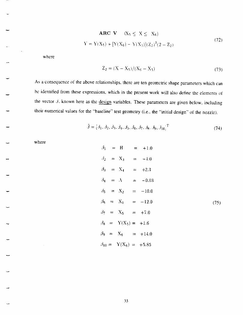
where

ARC V (Xs_< X < X6)

Y = Y(X_) + [Y(X6) - Y(X_)](Z2)3(2 - Z.,)(72)

Z, = (X- X_)/(X6 - X_) (73)

As a consequence of the above relationships, there are ten geometric shape parameters which can

be identified from these expressions, which in the present work will also define the elements of

the vector ,}. known here as the design variables. These parameters are given below, including

their numerical values for the "baseline" test geometry (i.e., the "initial design" of the nozzle).

where

,3 = [31 , 3'2, 33, 34, 35, 36, Jr. &, 39,310] T (74)

31 =

,32 =

33 =

!';_4 :

35 =

,]7 =

38 =

_39 =

_10 =

H = +1.0

X3 = -4.0

X4 = +2.3

A = -0.03

X2 = -10.0

X1 = -12.0

X5 = +7.0

Y(Xs) = +1.6

X6 = + 14.0

Y(X6) = +5.85

(75)

33

3.1.2 Calculation and Validation of Sensitivity Derivatives

A study is conducted to validate the methodology which has been described herein for

computing aerodynamic sensitivity derivatives, and to evaluate the efficiency of the procedures.

In this study, geometric shape sensitivity derivatives are calculated using direct solution of Eq.

(18) (together with some of the ancillary sensitivity equations presented in a previous sub-

section), and are also computed using the method of "brute force" finite differences. In applying

the method of finite differences, in order to insure great accuracy, central differences are used

(requiring two CFD analyses per design variable) with an extremely small perturbation of each

design variable, and the repeated CFD analyses are converged to machine zero. Sensitivity

derivatives taken with respect to the ten previously described geometric shape design variables

(Eqs. (65) through (75)) are computed using these two methods, and are compared in Tables I,

II, III, and IV. In Tables I and II, the sensitivity derivatives of Cx and Cy, respectively, for the

lower wall of the nozzle are presented (Cx and Cy are aerodynamic force coefficients in the x

and y directions, respectively, resulting from the integration of pressure and skin friction along

the wall, and have been detailed previously.) In Tables III and IV, the sensitivity derivatives of

the thrust, T, and the mass flow rate, rh, of the nozzle are given.

Design

Variable

31

J2

6/3

3a

X-Direction Force

Coefficient Sensitivity

Direct

Differentiation

-4.925 E+01

-4.614 E+02

+2.284 E+02

-2.665 E+04

Finite

Difference

-4.925 E+01

-4.614 E+02

+2.284 E+02

-2.665E+04

f15 -8.327 E+01 -8.327 E+01

36 -1.365 E-02 -1.365 E-02

37 +1.415 E+00 +1.415 E+00

¸.'38 +6.235 E+00 +6.235 E+00

,39 -2.107 E+00 -2.107 E+00

31o +3.886 E-01 +3.886 E-01

Table I - Comparison of the X-direction Force Coefficient, Cx, Sensitivity

Derivatives, Lower Wall, Double-Throat Nozzle, Laminar Flow

34

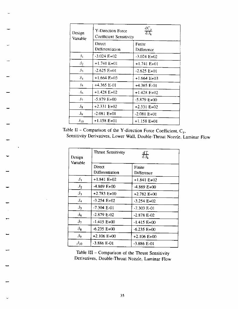
dCY-DirectionForce _,.DesignCoefficientSensitivityVariableDirect FiniteDifferentiation Difference

31 -3.024 E+02 -3.024 E+02

'32 +1.741 E+01 +1.741 E+O1

33 -2.625 E+OI -2.625 E+O1

:34 + i.664 E+03 + 1.664 E+03

35 +4.365 E-01 +4.365 E-OI

,36 + 1,428 E+02 + 1.428 E+02

37 -5.879 E+00 -5,879 E+O0

'38 +2.331 E+02 +2.331 E+02

39 -2.081 E+OI -2.081 E+O1

'31o +1.158 E+01 +1.158 E+OI

Table II - Comparison of the Y-direction Force Coefficient, Cy,

Sensitivity Derivatives, Lower Wall, Double-Throat Nozzle, Laminar Flow

Thrust Sensitivity dT

Design

VariableDirect Finite

Differentiation Difference

31 +1.841 E+02 +1.841 E+02

/32 -4.869 E+00 -4.869 E+00

33 .+2.783 E+00 +2.782 E+00

'34 -3.254 E+02 -3.254 E+02

35 -7.304 E-01 -7.303 E-01

/36 -2.879 E-02 -2.878 E-02

'37 -1.415 E+00 -1.415 E+00

3s -6.235 E+00 -6.235 E+00

;_9 +2.106 E+00 +2.106 E+00

/31o -3.886 E-01 -3.886 E-01

Table III - Comparison of the Thrust Sensitivity

Derivatives, Double-Throat Nozzle, Laminar Flow

35

driaMassFlowRateSensitivityDesign

VariableDirect FiniteDifferentiation Ditlerence

31 +5.701 E+00 +5.701 E+00

.32 - 1.639 E-02 - 1.639 E-02

33 +2,819 E-02 +2.819 E-02

34 -2.168 E+00 -2.168 E+00

•35 -1.933 E-05 -1.895 E-05

36 -1.172 E-(M -1.171 E-04

,37 -1.1)96 E-09 +0.000 E+00

J8 -4.158 E-09 -5.684 E-09

39 +1.131 E-04 +1.134 E-04

31o -8.740 E-13 +0.f)00 E+00

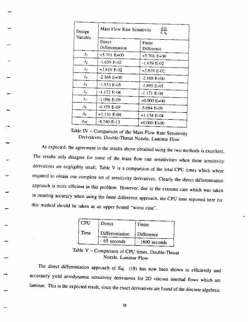
Table IV - Comparison of the Mass Flow Rate Sensitivity

Derivatives, Double-Throat Nozzle, Laminar Flow

As expected, the agreement in the results above obtained using the two methods is excellent.

The results only disagree for some of the mass flow rate sensitivities when these sensitivity

derivatives are negligibly small. Table V is a comparison of the total CPU times which where

required to obtain one complete set of sensitivity derivatives. Clearly the direct differentiation

approach is more efficient in this problem. However, due to the extreme care which was taken

in insuring accuracy when using the finite difference approach, the CPU time reported here for

this method should be taken as an upper bound "worst case".

CPU Direct Finite

Time Differentiation Difference

- 65 seconds - 1800 seconds

Table V - Comparison of CPU times, Double-Throat

Nozzle, Laminar Flow

The direct differentiation approach of Eq. (18) has now been shown to efficiently and

accurately yield aerodynamic sensitivity derivatives for 2D viscous internal flows which are

laminar. This is the expected result, since the exact derivatives are found of the discrete algebraic

36

equations which model the fluid flow. Unfortunately, however, a majority of the practicai flow

problems of interest in aerodynamic design are turbulent flows. If turbulence modeling is to be

included in the flow calculations, then in principle, the equations which are used in the turbulence

model which is selected should be consistently differentiated, and the results fully incorporated

into the Jacobian matrices, and 5"gx '

analysis equations (i.e., Eqs. (16) through (21)). In practice, of course, for typical turbulence

models, this represents a very difficult task, even impossible in the case of turbulence models

which are not continuously differentiable (e.g., the popular Baldwin-Lomax model). For this

reason, in typical CFD codes, consistent linearization of the turbulence modeling is neglected

in the construction of the implicit terms of the matrix, [a9--_], of Eq. (12)for the integration of

the equations in time. Of course, the explicit spatial variation of the turbulence modeling terms

which is found in the residual vector on the right-hand side of Eq. (12) is also used on the

[o jleft-hand side in the terms of the Jacobian matrix, _ .

As a potentially useful simplifying approximation in the calculation of sensitivity derivatives

for turbulent flows, an approach analogous to that described above for implicit time integration

schemes is proposed. That is, differentiation of the turbulence modeling is neglected in the

[< Iconstruction of the terms of the Jacobian matrices, , and g_- , of Eqs. (16) through (21).

The explicit spatial variation of the steady-state values of the turbulence modeling terms is used,

however, in both of these Jacobian matrices. This approximation is equivalent to a "locally

constant" assumption applied to these terms.

In order to judge the error in the sensitivity derivatives which might be expected in using this

approximation, a preliminary investigation is conducted using the present double-throat nozzle

problem, and the Baldwin-Lomax turbulence model [21]. Strictly speaking, this turbulence model

is not applicable to the present low Reynolds number problem, but this does not conflict with

the goals of this preliminary investigation into the effect of turbulence models on the accuracy

of the sensitivity derivatives.

37

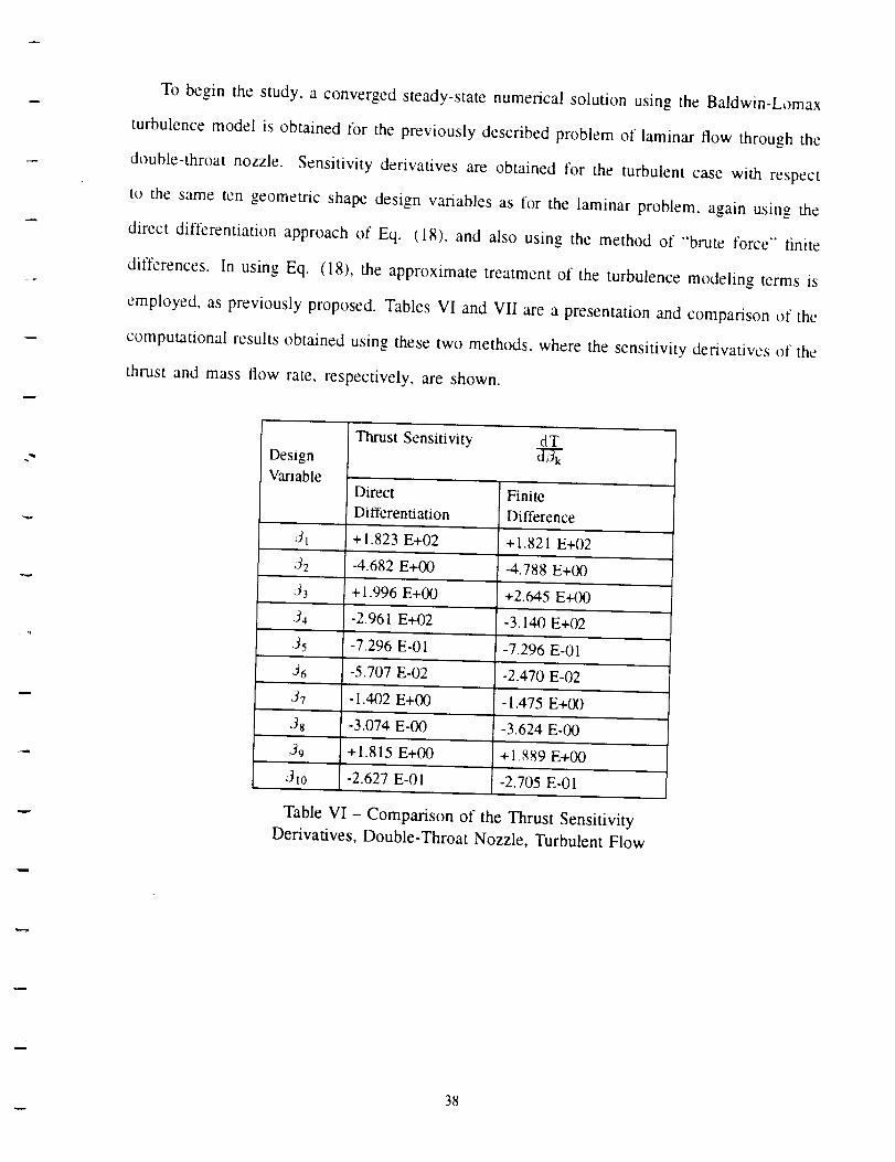
To begin the study, a converged steady-state numerical solution using the Baldwin-Lomax

turbulence model is obtained for the previously described problem of laminar flow through the

double-throat nozzle. Sensitivity derivatives are obtained for the turbulent case with respect

to the same ten geometric shape design variables as for the laminar problem, again using the

direct differentiation approach of Eq. (18), and also using the method of "brute force" finite

differences. In using Eq. (18), the approximate treatment of the turbulence modeling terms is

employed, as previously proposed. Tables VI and VII are a presentation and comparison of the

computational results obtained using these two methods, where the sensitivity derivatives of the

thrust and mass flow rate, respectively, are shown.

Thrust Sensitivity dTDesign

VariableDirect Finite

Differentiat.ion Difference

31 +1.823 E+02 +1.821 E+02

:J2 -4.682 E+00 -4.788 E+00

3 3 +1.996 E+00 +2.645 E+00

3_ -2.961 E+02 -3.140 E+02

_35 -7.296 E-0I -7.296 E-01

,36 -5.707 E-02 -2.470 E-02

37 - 1.402 E+00 - 1.475 E+00

;38 -3,074 E-00 -3,624 E-00

,39 +1.815 E+00 +1S89 E+00

31o -2.627 E-01 -2.705 E-01

Table VI - Comparison of the Thrust Sensitivity

Derivatives, Double-Throat Nozzle, Turbulent Flow

38

dmMass Flow Rate SensitivityDesign

VariableDirect Finite

Differentiation Difference

.3: +5.703 E+00 +5.697 E+00

.3,, - 1.699 E-02 - 1.641 E-02

,3: +2.894 E-02 +2.841 E-02

.34 -2.238 E+(X) -2.187 E+00

35 -2.317 E-05 -2.463 E-05

.36 -6.753 E-04 -1.516 E-04

37 -5,658 E-l0 +0,000 E+00

.38 -1.949 E-09 -4.263 E-09

09 +2.816 E-04 +1.045 E-04

3to -2.084 E-13 -1.421 E-09

Table VII -Comparison of the Mass Flow Rate Sensitivity

Derivatives, Double-Throat Nozzle, Turbulent Flow

Note that in generating the "brute force" sensitivity derivatives shown in Table VI and

VII, the same extreme care was taken to insure great accuracy of the terms that was taken

previously for the laminar results. Therefore, the "brute force" values shown for the turbulent

case are considered to be more accurate than the values obtained using the method of direct

differentiation (because of the approximate treatment of the turbulence modeling terms which

was used in the latter approach). In general, however, the agreement between the two methods

is reasonably good, hopefully good enough for future use in a design optimization strategy.

3.1.3 Optimization Problem -- Double-Throat Nozzle

Having verified the accuracy and efficiency of the methodology for computing sensitivity

derivatives, a short study is conducted to demonstrate the application of the sensitivity derivatives

in a model optimization example problem, using the double-throat nozzle described above. A

generalized procedure is proposed for aerodynamic design optimization, where the principal

computational tasks are sub-divided into distinct modules, or major subroutines, all controlled

by a central, external, general purpose design optimization computer program. The well-known

39

designoptimization programselectedfor use in the presentstudy is called ADS (Automated

DesignSynthesis),which is documentedin Ref. [48], althoughothersareavailable.

Theprincipalcomputationaltasksto beperformeddynamicallyin theautomatedaerodynamic

design strategy are accomplishedusing a standardCFD code (in order to re-evaluatethe

aerodynamicperformancevariables),a sensitivity analysisprogram,basedon theCFD analysis

code (for computing the sensitivity derivativesrequired by the optimization program),a grid

regenerationprogram (for shapeoptimization,as the shapeof the domain changes)and grid

sensitivity capability (necessaryin computingshapesensitivity derivatives). In addition, an

optional approximateanalysiscapability (basedon Eqs. (19) or (21), for geometricshape

changes)can be includedas a subsetof the sensitivity analysismodule, in order to provide

significantly more efficient re-evaluationof the aerodynamicperformancevariables,when the

changesin thedesignvariablesaresmall (i.e., lessthansomespecifiedtolerance).The validity,

accuracy,and efficiency of the approximateanalysis methodologyis documentedin Refs.

[3,5,6,7]. The proposedaerodynamicdesignoptimization strategyis illustrated in Fig. (10).

Startingwith the initial nozzleshapeand steady-statesolution, th, proposedaerodynamic

shapeoptimizationmethodof Fig. (10) is appliedto the nozzleproblem,as follows:

1) Theforcecoefficientin thex direction,Cx,(henceforthknownastheobjective function),

is to be minimized in th e design, subject to the explicit constraints on the design variables,

"given subsequently. Cx represents the internal aerodynamic drag on the lower wall of

the nozzle.

2) The design variables are the ten elements of 5, defined in Eq. (75), and an upper and

lower bound is placed on each, where the total maximum allowable change in each

during the design, either an increase or decrease, is specified a priori to be no greater

than 15% of the initial value of each variable.

3) Sensitivity derivatives with respect to the design variables of the objective function are

obtained using the method of direct differentiation (Eq. (18)) and the ancillary sensitivity

equations given previously. Sensitivity derivatives of the explicit constraints (i.e., the

40

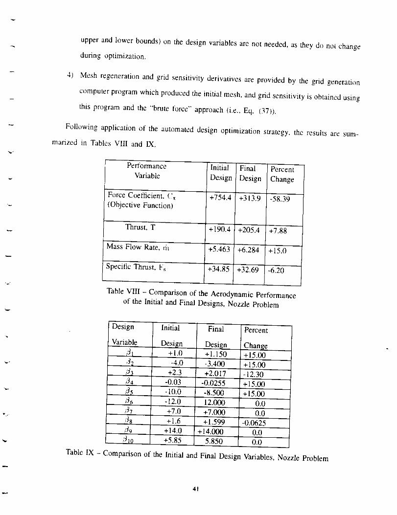
upperandlower bounds)on thedesignvariablesarenot needed,astheydo not change

during optimization.

4) Meshregenerationand grid sensitivityderivativesare providedby the grid generation

computerprogramwhichproducedtheinitial mesh,andgrid sensitivityisobtainedusing

this programand the "brute force" approach(i.e., Eq. (37)).

Following applicationof the automateddesignoptimizationstrategy,the resultsaresum-

marizedin TablesVIII and IX.

"7

Performance

Variable

Force Coefficient. L'x

(Objective Function)

Initial

Design

Mass Flow Rate, ri_

Sp'ecific Thrust. Fs

+754.4

Final

Design

+313.9

Percent

Change

-58.39

Thrust, T +190.4 +205.4 +7.88

+5.463 +6.284 +15.0

+34.85 +32.69 -6.20

Table VIII - Comparison of the Aerodynamic Performance

of the Initial and Final Designs, Nozzle Problem

Design

Variable

32

33_4

_6

A7

,3S

31o

Initial

Design

+l.0

-4.0

+2.3

-0.03

Final

Design+1.150

-3.400

+2.017

-0.0255

Percent

Change

+15.00

+15.00

-12.30

+15.00

-10.0 -8.500 +15.00

- 12.0 12.000 0.0

+7.0 +7.000 0.0

+ 1.6 + 1.599 -0.0625

+14.0 +14.000 0.0

+5.85 5.850 0.0

Table IX - Comparison of the Initial and Final Design Variables, Nozzle Problem

4l

Clearly a significant reduction in the aerodynamic drag on the internal walls of the nozzle (as

defined in the present problem statement) was achieved, as demonstrated by the desired reduction

in the objective function in the new design. Figs. (1 la) and (1 lb) represent a comparison of

the geometric shapes of the initial and final nozzle designs, respectively. (Fig. (1 la) is a repeat

of Fig. (7).) In reducing the aerodynamic drag on the internal walls of the nozzle, the shape

of the final design clearly displays a predictable pattern of "smoothing out the bumps" in the

contours of the wails. Had the explicit bounds on the design variables been removed, this

effect would surely have been even greater. The results shown here were obtained following

only three evaluations of the objective function (following the initial evaluation). The option of

approximate analysis was not used in the present test problem.

In the present model design problem, aerodynamic drag reduction is considered, as it is

of general interest in many aerodynamic design problems. In the design of nozzles, however,

clearly the thrust, mass flow rate, and specific thrust, Fs, (Fs = T/th) are variables of special

interest to the designer. For this reason, the values of these variables for the initial and final

designs have been included in Table VIII. A more realistic shape optimization problem for

nozzles might typically select the maximization of Fs as the objective function, perhaps with

the side constraint that the thrust of the final design be no less than that of the initial design.

Reformulation of the present test problem in this manner is straightforward, in principle, since

the sensitivity derivatives of these terms are available (i.e., thrust and mass flow rate sensitivities

have been presented herein, from which specific thrust sensitivities are obtained using Eq. (64).

3.2 External Flow -- NACA 4-Digit Airfoil Problem

3.2.1 Description of the Test Problem

The external flow problem which is studied in the present work is that of an isolated airfoil.

The initial airfoil which is selected is the NACA 2412, the profile of which is defined by Eqs.

(41) and (42), with maximum thickness, T = 0.12, maximum camber, C = 0.02, and location of

maximum camber, L = 0.40. The computations are performed on a "C" mesh using 128 points

42

in the"aroundtheairfoil" direction,(with 68of theseon thesurfaceof the airfoil) and32points

in the normal to the airfoil direction,with grid stretchingnearthe airfoil surface.The far-field

boundaryis placedtwentychordsfrom theairfoil. The grid is generated using the algebraic mesh

generation program of Ref. [42]. The grid used in the present test case is clearly inadequate

for use in resolving the full physics of viscous flow over an airfoil. Therefore, it should be

understood that the objective of the work for which results are to be presented is no....3tat this point

to produce highly accurate calculations of the flow field. The objective rather is to successfully

implement, demonstrate, and validate the ideas on a computationally inexpensive model problem.

A converged conventional numerical solution is obtained for the initial geometry and grid for

laminar flow, for a freestream Mach number, XI_ = 0.70, Reynolds number, REt, = 5000., and

angle of attack a = 0.0 °. Boundary conditions on the airfoil surface, across the "wake-cut", and

at the far-field boundaries have been discussed previously. When the "lift corrected" far-field

boundary conditions are no_.__!tused, the lift (CL), drag (CD), and moment (CM) coefficients for the

calculation were CL = 0.1232, CD = 0.06824, and CM = - 0.05328. When the lift correction

of Ref. [40] is applied at the far-field boundaries, these coefficients become CL = 0.1252, CD

= 0.06821, and CM = - 0.05325. Therefore, the numerical effect of the far-field lift correction

is not strong in this example problem, which is attributed to the rather large extent of the far-

field boundary from the airfoil (twenty chords) which was used. This effect will become more

significant, however, as the far-field boundary is brought closer to the airfoil surface [40], i.e..

the lift-corrected boundary conditions become more necessary. Of course, the freedom to move

the far-field boundary closer to the airtbil surface allows more effective use of the grid points

which are available, in order to more accurately resolve the flow physics.

3.2.2 Calculation and Validation of Sensitivity Derivatives

A study is conducted to validate the methodology which has been described herein tbr

computing aerodynamic sensitivity derivatives for airfoils, and to evaluate the efficiency of

the procedures. Unless otherwise stated, sensitivity derivatives are computed using the steady-

state solution without the point-vortex lift-corrected far-field boundary conditions. In particular,

43

geometricshapesensitivity derivativesarecalculatedby solutionof Eq. (18) using the hybrid

direct solver / iterative strategy proposed in Eq. (30) (and also using some of the ancillary

sensitivity equations presented previously). For comparison purposes, the sensitivity derivatives

are also computed using the "brute force" method of finite differences. In applying this approach,

to insure good accuracy, central finite difference approximations are used with a forward and

backward perturbation of each design variable of 0.01%, and the repeated CFD analyses are

converged to machine zero.

The sensitivity derivatives of the lift, drag, and moment coefficients are computed with

respect to the three geometric shape parameters, T, C, and L of Eqs. (41) and (42) using

the initial airfoil, grid, and flow conditions which have been described immediately above.

In solving Eq. (18), the required grid sensitivity terms (i.e., _j_)were provided using

the previously described "elastic membrane" representation of the computational domain, and

the prescribed displacement approach, together with Eqs. (39) through (45). In addition,

as a consistency requirement, this grid methodology is also used in generating the necessary

"'perturbed" grids which are required in computing aerodynamic sensitivity derivatives by the

"'brute force" approach.

When solving Eq. (18) using the hybrid direct solver / iterative method of Eq. (30), it

is necessary to establish some type of criterion by which the iterative solution of the linear

system for each design variable is judged to be "converged," and is terminated. To study this,

the sensitivity derivatives are calculated with E,q. (30) using progressively stricter convergence

criteria, starting with a calculation where no iterations are used (i.e., the "'periodic" terms outside

of the central bandwidth are simply neglected) and ending with a calculation where the average

global error is reduced four orders-of-magnitude. A summary of these calculations, including

the results of the finite difference approach, is presented in Tables X, XI, and XII, one table for

each of the three geometric shape design variables, T, C, and L, respectively.

As expected, as the reduction in the error by the iterative process defined by Eq. (30) is

increased, the agreement between the sensitivity derivatives calculated using the method of direct

44

differentiation (Eq. (18)) and the sametermscalculatedusing the methodof finite ditfetences

is excellent. In addition, the validity of the "elastic membrane"methodologyfor computing

grid sensitivitiesis confirmed. Furthermore,in thepresentproblem, it is demonstratedthat 1)

approximatelya threeorders-of-magnitudereductionin the error is more thansatisfactoryfor

engineeringpurposesin applying Eq. (30), but 2) completeneglectof the implicit periodic

boundaryconditiontermsis completelyunacceptablein usingEq. (18) to predict thesensitivity

derivatives (Note: In contrast, these terms typically are neglected in the integration of the

equations in time, using Eq. (12)).

Method

of

Solution

Lift Sensitivity

O& = "

Drag Sensitivityoc_ _ oc:D031 -- 0T

Moment Sensitivityoc_ _ ac_.q.a.03_ -- OT

No. of

Iterations

Using Eq. (30)

Eq. (30),

Without -9.334 E-01 +4.723 E-OI +9.815 E-02 1

Iterations

Eq, (30),

10M -2.859 E+O0 +4.267 E-O1 +4.755 E-OI 13

Eq. (30),

20M -3.117 E+O0 +3.972 E-01 +5.278 E-O1 64

Eq. (30),

30M -3.126 E+O0 +3.939 E-O1 +5.307 E-OI 219

Eq. (30),

40M -3.126 E+O0 +3.938 E-01 +5.307 E-OI 300

Finite

Difference -3.126 E+OO +3.938 E-01 +5.307 E-OI N/A

*OM Refers to the number of Orders-of-Magnitude reduction in the average global error.

Table X - Comparison of Lift and Drag Sensitivity Derivatives

With Respect To Maximum Thickness, 31 =T, NACA 2412 Airfoil

45

Method

of

Solution

Lift Sensitivityocq.a _ _c2s.:)3_ -- :)C

Drag Sensitivity

-- "]C

Moment Sensitivity_-_:)J2 -- ,]C032

Eq. (30),

Without +5.206 E+O0 +3.429 E-OI -2.520 E+O0 1

Iterations

Eq. (30),

10M +4.175 E+00 +3.780 E-01 -2.261 E+00 14

Eq (30),

2 ()M +3.988 E+00 +3.663 E-01 -2.225 E+00 39

Eq. (30),

30M -.-3.968 E+00 +3.603 E-01 -2.220 E+00 188

Eq. (30),

4 OM +3.968 E+00 +3.603 E-01 -2.220 E+00 276

Finite

Difference +3.968 E+00 +3.603 E-01 -2.220 E+00 N/A

No. of

Iterations

Using Eq. (30)

*OM Refers to the number of Orders-of-Magnitude reduction in the average global error.

Table XI - Comparison of Lift and Drag Sensitivity Derivatives

With Respect To Maximum Camber, 32---C, NACA 2412 Airfoil

Method

of

Solution

Lilt Sensitivity

")is -- ,gL

Drag Sensitivity Moment Sensitivity

'J']3 -- ,')L ,gJ_ -- ,'gL

No. of herations

Using Eq. (30)

Eq. (30),

Without -4.293 E-02 -3.899 E-03 -3.865 E-02 1

Iterations

Eq. <30),

1 OM -1.466 E-02 -3.422 E-03 -4.456 E-02 5

Eq. (30),

2 OM -1.869 E-02 -3.334 E-03 -4.386 E-02 24

Eq. (30),

3 OM -1.819 E-02 -3.304 E-03 -4.396 E-02 49

Eq. (30),

4 OM -1.816 E-02 -3.290 E-03 -4.398 E-02 195

Finite

Difference -1.815 E-02 -3.290 E-03 -4.398 E-02 N/A

*OM Refers to the number of Orders-of-Magnitude reduction in the average global error.

Table XII - Comparison of Lift and Drag Sensitivity Derivatives With

Respect To Location of Maximum Camber, .33=L, NACA 2412 Airfoil

46

Table XIII is a comparison of the relative computational cost of obtaining the sensitivity

derivatives using the procedures for which results have been given in the three preceding tables.

In the present problem, clearly the finite difference method is less efficient than the use of Eq.

(30), even when the required error reductions using Eq. (31)) are specified to be large. However,

because of the great care which was taken in applying the finite difference method to insure

very accurate results (for validation purposes), the CPU times reported for this finite difference

method should be taken to represent a "worst case" scenario.

Method of CPU Time, Total

Solution (seconds)

Eq. (30), Without 27

Iterations

Eq. (3O) 33

10M

Eq. (30) 5420M

Eq. (30) 124

30M

Eq. (30) 191

40M

Finite 840

Difference

*OM Refers to the number of Orders-of-Magnitude reduction in the average global error.

Table XIII - Comparison of CPU Times - Airfoil Problem

As mentioned earlier, in applying the hybrid direct solver / iterative strategy of Eq. (30)

in the solution of Eq. (18), for the results presented above, it was necessary to use under-

relaxation to force the iterations to converge. A single under-relaxation parameter, _ = 0.75

was used. The required use of this parameter, in addition to the relatively large numbers of

iterations (and hence the proportionally large amounts of CPU time) required in reducing the

error to an acceptable level is worrisome, and was neither the expected nor the desired result.

As stated earlier, these difficulties were not encountered in the related work of Ref. [33,39].

Additional work is needed to correct these difficulties, and to improve the efficiency of the

algorithms for solving the equations of sensitivity analysis. Recent studies have cast these large

47

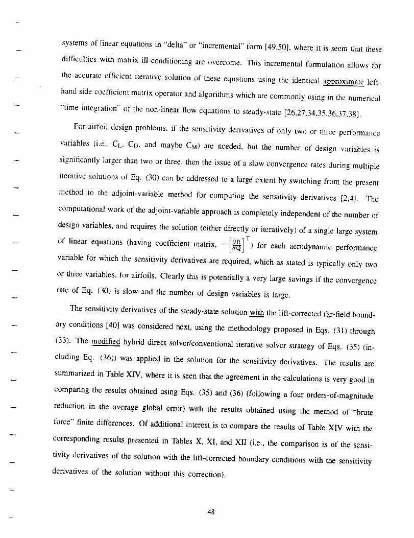
systemsof linearequationsin "delta" or "incremental" form [49,50], whereit is seemthat these

difficulties with matrix ill-conditioning areovercome.This incremental formulation allows for

the accurate efficient iterative solution of these equations using the identical approximate left-

hand side coefficient matrix operator and algorithms which are commonly using in the numerical

"time integration" of the non-linear flow equations to steady-state [26,27,34,35,36,37.38].

For airfoil design problems, if the sensitivity derivatives of only two or three performance

variables (i.e., CL, CD, and maybe CM) are needed, but the number of design variables is

significantly larger than two or three, then the issue of a slow convergence rates during multiple

iterative solutions of Eq. (30) can be addressed to a large extent by switching from the present

method to the adjoint-variable method for computing the sensitivity derivatives [2,4]. The

computational work of the adjoint-variable approach is completely independent of the number of

design variables, and requires the solution (either directly or iteratively) of a single large system

of linear equations (having coefficient matrix, - ) for each aerodynamic performance

variable for which the sensitivity derivatives are required, which as stated is typically only two

or three variables, for airfoils. Clearly this is potentially a very large savings if the convergence

rate of Eq. (30) is slow and the number of design variables is large.

The sensitivity derivatives of the steady-state solution wit_.__hthe lift-corrected far-field bound-

ary conditions [40] was considered next, using the methodology proposed in Eqs. (31) through

(33). The modified hybrid direct solver/conventional iterative solver strategy of Eqs. (35) (in-

cluding Eq. (36)) was applied in the solution for the sensitivity derivatives. The results are

summarized in Table XIV, where it is seen that the agreement in the calculations is very good in

comparing the results obtained using F_,qs. (35) and (36) (following a four orders-of-magnitude

reduction in the average global error) with the results obtained using the method of "brute

force '_ finite differences. Of additional interest is to compare the results of Table XIV with the

corresponding results presented in Tables X, XI, and XlI (i.e., the comparison is of the sensi-

tivity derivatives of the solution with the lift-corrected boundary conditions with the sensitivity

derivatives of the solution without this correction).

48

Solution

Method

Eqs (35)and (36),

40M*

"Brute Force."

FiniteDifference

Method.

Design

Variable

T

dCLdT.C, L

-3.211E+O0

dCDdT. C. L

+3.959E-01

dC.,adT. C. L

+5.337E-01

C +4.015E+00 +3.578E-01 -2.216E+00

L -1.751E-02 -3.327E-03 -4.410E-02

-3.211E+O0

-4.o15 E+O0

T +3.959 E-01 +5.337 E-01

C +3.578 E-01 -2.217 E+_X)

L -1.752 E-02 -3.326 E-03 -4.410 E-02

*OM Refers to the number of Orders-of-Magnitude reduction in the average global error.

Table XIV - Comparison of the Sensitivity Derivatives With The

Lift-Corrected Far-Field Boundary Conditions - Airfoil Problem

3.2.3 Optimization Problem -- NACA 4-digit Airfoil

Having successfully validated the accuracy and efficiency of the proposed strategies for

computing grid regeneration, grid sensitivity derivatives, and finally, aerodynamic sensitivity

derivatives for isolated airfoils on "C" and "O" meshes, the application of these methods is

demonstrated here in a model airfoil design optimization problem. The optimization strategy

described previously for the nozzle test problem (and illustrated in Fig. (10)) is applied, using

the NACA 2412 airfoil, grid, and steady-state solution described above as the initial design. The

optimization problem is formulated as follows:

1) The lift coefficient, Ct., is to be maximized in response to geometric shape variations,

subject to the design constraints defined subsequently.

2) The drag coefficient, CD, is to be no greater than the value of the initial design.

3) The design variables (i.e., the elements of 2) are the three parameters of the NACA

4-digit airfoil, i.e., T, C, and L, defined previously. The "linearized" NACA 4-digit

49

airfoil of Eqs. (.43)and (44) definesthe rangeof allowable airfoil shapesin termsof

thesethreeparameters.(As statedpreviously,this linearizedequationonly approaches

the true NACA 4-digit parameterizationof Eqs. (41) and (42) for small changesin

the parameters,but the current parameterizationis no._.._tlimited to small changes). In

addition,upperand lower boundsaredefineda priori, for eachof thedesignvariables.

as tbllows:

0.08< T < 0.16

0.00_ (' < O.O,5

0.20< L < 0.60

4) Sensitivityderivativesof theobjectivefunction,CL, andtheconstraint,Co, with respect

to thedesignvariablesareobtainby solutionof Eq. (18),usingthe hybrid direct solver

/ iterative strategy of Eq. (30). The global average error reduction in the solution of Eq.

(18) is specified to be three orders-of-magnitude for each design variable. Sensitivity

derivatives of the explicit constraints on the design variables (i.e., the upper and lower

bounds) are not needed.

5) Mesh regeneration and grid sensitivity derivatives are provided dynamically during the

automated optimization process using the finite element method and the "elastic mem-

brane" prescribed displacement model of the computational grid, presented previously.

One important benefit and use of sensitivity analysis is the ability to study the sensitivity

derivatives of the initial design before the design process begins, in order to identify which

design variables are important (i.e., very sensitive) to the problem, and which are not. By

this, often it can be safely judged that some of the design variables are unneeded, and can be

eliminated from the problem.

As an example of this, examination of the sensitivity derivatives in Tables X, XI, and XII (or

Table XIV) reveals that the lift and drag sensitivities are about two orders-of-magnitude smaller

for the third design variable, L, compared to the sensitivity derivatives for the remaining two.

5O

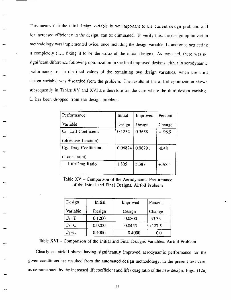
This meansthat the third designvariableis not importantto the currentdesignproblem,and

for increasedefficiency in thedesign,canbeeliminated.To verify this, thedesignoptimization

methodologywasimplementedtwice,onceincluding thedesignvariable,L, andonceneglecting

it completely(i.e., fxing it to be the value of the initial design). As expected,therewas no

significantdifferencefollowing optimizationin thefinal improveddesigns,eitherin aerodynamic

pertbrmance,or in the final valuesof the remaining two design variables,when the third

designvariablewasdiscardedfrom the problem. The resultsof the airfoil optimization shown

subsequentlyin TablesXV andXVI are thereforefor thecasewherethe third designvariable.

L, hasbeendroppedfrom the designproblem.

Performance

Variable

eL, Lift Coefficeint

(objective function)

CD, Drag Coefficient

(a constraint)

Lift/Drag Ratio

Initial

Design

0.1232

0.06824

1.805

Improved

Design

0.3658

0.06791

5.387

Percent

Change

+196.9

-0.48

+198.4

Table XV - Comparison of the Aerodynamic Performance

of the Initial and Final Designs, Airfoil Problem

Design Initial Improved Percent

Variable Design Design Change

/31=T 0.1200 0.0800 -33.33

32--C 0.0200 0.0455 +127.5

33=L 0.4000 0.4000 0.0

Table XVI - Comparison of the Initial and Final Designs Variables, Airfoil Problem

Clearly an airfoil shape having significantly improved aerodynamic performance for the

given conditions has resulted from the automated design methodology, in the present test case,

as demonstrated by the increased lift coefficient and lift / drag ratio of the new design. Figs. (12a)

51

and (12b) representa comparisonbetweenthe geometricshapesof the initial and final airfoil

designs,respectively.The resultsshownherewereobtainedfollowing only two evaluationst_f

theobjectivefunction(following theinitial evaluation).Theoptionof approximateanalysiswas

not usedin the presenttest problem.

4.0 Summary and Conclusions

A gradient based design optimization strategy has been developed in detail for use in practical

aerodynamic design problems, using the 2D thin-layer Navier-Stokes equations. The strategy

is general in nature, and is based on the classic idea of constructing different modules for

performing the major tasks such as function evaluation, function approximation and sensitivity

analysis, mesh regeneration and grid sensitivity analysis, all driven and controlled by a general

purpose design optimization program. The methodology has been successfully demonstrated on

both an internal and an external flow problem, where in each case, a significant improvement

in aerodynamic performance was achieved.

In developing the methods which have been presented herein, the major effort has been lb-

cused on techniques for efficiently and accurately calculating the necessary sensitivity derivatives

for use by the optimization program. In particular, much effort was spent in successfully devel-

oping and implementing a consistent treatment of the boundary conditions in the calculation of

the aerodynamic sensitivity derivatives for the classic problem of external flow over an isolated

lifting airfoil on "C" or "O" meshes. As a minor extension of the methodology for computing

the sensitivity derivatives, an efficient strategy for approximate analysis is available, a capability

which is potentially very useful in a design environment.

One of the most difficult design variables to consider is that of geometric shape, which

has been the emphasis of the present work. With geometric shape, the issue of grid sensitivity

analysis and grid regeneration must be considered in the development of an automated gradient

based optimization scheme. In the present work, an efficient method for handling this difficulty

based on well-known ideas from the discipline of structural shape design optimization has been

52

successfullyapplied to the aerodynamicdesign problem. The technique employs the hnite

element method, and an elastic membrane representation of the computational domain.

The investigation which has been presented herein is still in its initial stages, and there is

an unlimited amount left to be done. For example, for the viscous airfoil problem which was

presented herein, the grid was of insufficient size to truly resolve the full physics of a viscous

flow. Future work will focus on implementation of the methods demonstrated here to full scale

grids. A more complete parameterization of the airtbil boundary with more design variables is to

be used. in order to increase the range of the design space. Design with turbulence modeling will

be attempted. Finally. development of more efficient strategies (with respect to computational

work and computer storage) for computing the sensitivity derivatives is underway.

5.0 Acknowledgments

This research was supported by grant number NAG-l-1265 from NASA Langley Research

Center with Dr. Henry E. Jones as the technical monitor. Contributions to the work through

helpful discussions were made by Dr. Perry A. Newman, Dr. Manuel Salas, and Dr. E. Carson

Yates, Jr. of NASA Langley. Ms. Sheila Belcher was the typist lbr the article.

6.0 References

1. Tayl_)r, A.C. III, Hou, G.W., and Korivi, V.M., "Sensitivity Analysis, Approximate Analysis,

and Design Optimization for Internal and External Viscous Flows," AIAA Paper 91-3083.

2. Hou, G.W., Taylor, A.C. III, and Korivi, V.M., "Discrete Shape Sensitivity Equations For

Aerodynamic Problems," AIAA Paper 91-2259.

3. Taylor, A.C. HI, Korivi, V.M., and Hou, G.W., "Sensitivity Analysis Applied to The Euler

Equations: A Feasibility Study with Emphasis on Variation of Geometric Shape," AIAA

Paper 91-0173, also, "A Taylor's Series Expansion of Geometric Shape Variation tbr The

Euler Equations," to appear AIAA Journal, September 1992.

4. Taylor, A.C. III, Hou, G.W., and Korivi, V.M., "A Methodology for Determining Aerody-

namic Sensitivity Derivatives With Respect to Variation of Geometric Shape," Proceedings

of the AIAA/ASME/ASCEIAHSIASC 32nd Structures, Structural Dynamics, and Materials

Conference, April 8-10, Baltimore, MD, AIAA Paper 91-1101, also "A Methodology for

Calculating Aerodynamic Sensitivity Derivatives," to appear, AIAA Journal.

53

5. Taylor, A.C,, III. Korivi, V.M., and Hou, G.W. "Approximate Analysis and SensitivityAnalysis MethodsFor ViscousFlow Involving Variationof GeometricShape,"Proceedings

of the AIAA t0th Computational Huid Dynamics Conference, June 24-26, 199l. Honolulu.

Hawaii. AIAA Paper 91-1569.

6. Taylor, A.C. III, Hou, G.W., and Korivi, V.M.. "An Efficient Method For Estimating Steady-

State Numerical Solutions to the Euler Equations", AIAA Paper 91-1680.

7. Korivi, V.M., "'Sensitivity Analysis Applied to the Euler Equations," M.S. Thesis, Old

Dominion University, Norfolk, VA, December, 1991.

8. Sorensen. TM., "Viscous Airfoil Optimization Using Conformal Mapping Coefficients as

Design Variables." M.S. Thesis, Department of Aeronautics and Astronautics. Massachusetts

Institute of Technology. June. 1991.

9. Yates. E.C.. Jr.. and Desmarais, R., "'Boundary Integral Method for Calculating Aerodynamic

Sensitivities with Illustration for Lifting Surface Theory," in Proceedings of the International

Symposium of Boundary Element Methods (IBEM 89), published by Springer-Verlag, Oct.

2-4, 1989, East Hartford, Conn.

10. Elbanna, H.M., and Carlson, L.A., "'Determination of Aerodynamic Sensitivity Coefficients

in the Transonic and Supersonic Regimes," Journal of Aircraft, Vol. 27, No. 6. June 1990,

pp. 507-518, also AIAA Paper 89-0532.

11. Yates, E.C., Jr., "Aerodynamic Sensitivities From Subsonic, Sonic, and Supersonic Unsteady,

Nonplanar Lifting-Surface Theory," NASA TM-100502, September, 1987.

12. Sobieszczanski-Sobieski, J., "The Case For Aerodynamic Sensitivity Analysis". In Sensi-

tivity Analysis in Engineering, NASA CP-2457, 1987.

13. Bristow, D.R., and Hawk, J.D., "Subsonic Panel Method For The Efficient Analysis of

Multiple Geometry Perturbations," NASA CP-3528, 1982.

14. Jameson, A., "Aerodynamic Design Via Control Theory," NASA CR-181749, also ICASE

Report No. 88-64, November, 1988, also Journal ,.i Scientific Computing, Vol. 3, pp.

233-260. 1988.

15. Frank P.D., and Shubin, G.R., "A Comparison of Optimization-Based Approaches for

a Model Computational Aerodynamics Design Problem," Applied Mathematics Technical

Report. ECA-TR-136-R1, Boeing Computer Services, Seattle, Washington, October, 1990,

also to appear, Journal of Computational Physics.

16. Shubin, G.R., and Frank, P.D. "A Comparison of the Implicit Gradient Approach and

the Variational Approach to Aerodynamic Design Optimization," Applied Mathematics and

Statistics Technical Report, AMS-TR-163, Boeing Computer Services, Seattle, Washington,

April, 1991.

17. Shubin, G.R., "Obtaining 'Cheap' Optimization Gradients from Computational Aerodynam-

ics Codes", Applied Mathematics and Statistics Technical Report, AMS-TR-164. Boeing

Computer Services, Seattle, Washington, June 1991.

54

18. Baysal, O. and Eleshaky, M.E., "Aerodynamic Sensitivity Analysis Methods for the Com-

pressible Euler Equations," Recent Advances in Computational Fluid Dynamics, (ed. O.

Baysal), ASME-FED Vol. 103, 1 lth Winter Annual Meeting, November, 1990, pp. 191-202.

19. Baysal, O., and Eleshaky, M.E., "Aerodynamic Design Optimization Using Sensitivity

Analysis and Computational Fluid Dynamics," AIAA Paper 91-0471.

20. Baysal, O.. Eleshaky, M.E.. and Burgreen, G.W.. "Aerodynamic Shape Optimization Using

Sensitivity Analysis on Third-Order Euler Equations." Proceedings of the AIAA 10th

Computational Fluid Dynamics Conference, June 24-26, 1991. Honolulu. Hawaii. AIAA

Paper 91-1577.

21. Baldwin. B.. and Lomax, H., "'Thin-Layer Approximation and Algebraic Model for Separated

Turbulent Flows." AIAA Paper 78-I)257.

22. Waiters, R.W.. and Thomas, J.L., "Advances in Upwind Relaxation Methods." in State of the

Art Surveys of Computational Mechanics, ed. A.K. Noor, pp. 145-183, ASME Publication,

1989, New York.

23. Thomas, J.L.. Van Leer, B., and Waiters, R.W., "Implicit Flux-Split Schemes for the Euler

Equations," AIAA Journal, Vol. 28, No. 6, June 1990, pp. 973-974, also AIAA Paper85-1680.

24. Waiters, R.W., and Dwoyer, D.L., "An Efficient Iteration Strategy for Solution of the Euler

Equations," AIAA Paper 85-1529.

25. Newsome, R.W., Waiters, R.W., and Thomas, J.L., "'An Efficient Iteration Strategy for

Upwind/Relaxation solutions to the Thin-Layer Navier-Stokes Equations," AIAA Journal.

Vol. 27, No. 9, September, 1989, pp. 1165-1166, also AIAA Paper 87-1113.

26. Thomas, J.L.. and Waiters, R.W., "Upwind Relaxation Algorithms for the Navier-Stokes

Equations," AIAA Journal, Vol. 25, No. 4, April 1987, pp. 527-534.

27. Napolitano, M., and Waiters, R.W., "An Incremental Block-Line-Gauss-Seidel Method for

the Navier-Stokes Equations, AIAA Journal, Vol. 24, No. 5, May 1986, pp. 770-776.

28. Waiters, R.W., and Dwoyer, D.I., "Efficient Solutions to the Euler Equations for Supersonic

Flow with Embedded Subsonic Regions," NASA Technical Paper 2523, January 1987.

29. Van Leer, B., "Flux-Vector Splitting for the Euler Equations," ICASE Report 82-30,

September 1982 (also Lecture Notes in Physics, Vol. 170, 1982, pp. 507-512).

30. Taylor, A.C. III, "Convergence Acceleration of Upwind Relaxation Methods For The Navier-

Stokes Equations," Ph.D. Dissertation, Virginia Polytechnic Institute and State University,

Blacksburg, VA, July, 1989.

31. Riggins, D.W., Waiters, R.W., and Pelletier, D., "The Use of Direct Solvers for Compressible

Flow Computations," AIAA Paper 88--0229.

32. Hafez, M., Palaniswamy, S., and MariaN, P., "Calculations of Transonic Flows with Shocks

Using Newton's Method and Direct Solver, Part II," AIAA Paper 88-0226.

55

33. Venkatakrishnan,V., "Newton Solutionof Inviscid and ViscousProblems",AIAA Journal

Vol. 27, No. 7, July 1989, pp. 885-891, also AIAA Paper 88-0413.

34. Beam, R.M. and Warming, R.F., "An Implicit Factored Scheme for the Compressible Navier-

Stokes Equations." AIAA Journal, Vol. 16, April 1978. pp. 393--402.

35. Taylor. A.C., III, Ng, W.F., and Waiters, R.W., "Upwind Relaxation Algorithms for the

Navier-Stokes Equations Using Inner Iterations," Proceedings of the AIAA 9th Computa-

tional Fluid Dynamics Conference, June 13-15, 1989, Buffalo, New York, AIAA Paper

89-1954, also Journal of Computational Physics, Vol. 99, No. 1, March 1992, pp. 68-78.

36. Waiters, R.W., Dwoyer. D.L., and Hassan, H.A.. '% Strongly Implicit Procedure for the

Compressible Navier Stokes Equations," AIAA Journal, Vol. 24, No. l. January 1986,

pp. 6-12.

37. Ajmani, K.. Ng, W.F., and Liou, M.S., "'Generalized Conjugate-Gradient Methods for the

Navier-Stokes Equations", Proceedinzs of the AIAA 10th Computational Fluid Dynamics

Conference, June 24-26, 1991 Honululu, Hawaii, AIAA Paper 91-1556.

38. Venkatakrishnan, V., "Preconditioned Conjugate Gradient Method For The Compressible

Navier-Stokes Equations", AIAA Journal, Vol. 29, No. 7, July, 1991, pp. 1092-t1(R), also

AIAA Paper 90--4)586.

39. Venkatakrishnan, V., NASA Ames Research Center, Private Communication.

40. Thomas, J.L, and Salas M.D., "Far-Field Boundary Conditions for Transonic Lifting Solu-

tions to the Euler Equations", AIAA Journal Vol. 27, No. 7, July 1986, pp. 1074-1080,

also AIAA Paper 85-0020.

41. Smith, R.E., Jr., and Sadrehaghighi, I., "Grid Sensitivity in Airplane Design," in Proceedings

of the 4th International Symposium of Computational Fluid Dynamics, September 9-12

1991, University of California-Davis, pp. 1071-1077.

42. Smith, R.E., Jr., and Wiese, M.R., "Interactive Algebraic Grid-Generation Technique,"

NASA TP-2533, March 1986.

43. Rajah, S.D., and Belegundu, A.D. "A Shape Optimization Approach Using Fictitious

Loads As Design Variables," Proceedings of the AIAA/ASME/ASCE/AHS 281h Structures.

Structural Dynamics_ and Materials Conferences," April 6-8, 1987, Monterey, CA, also

AIAA Paper 87-0834.

44. Choi, K.K., and Yao, T.M., "3-D Modelling and Automatic Regridding in Shape Design

Sensitivity Analysis," in Sensitivity Analysis in Engineering, NASA Conference Publication

2457, September, 1986, pp. 329-346.

45. Viviand, H., "Comparison of Numerical Solutions to Internal Flow in a Double-Throat

Nozzle," GAMM Committee for Numerical Methods in Fluid Mechanics, France, December,

1985.

46. Thomas, J.L., Waiters, R.W., Van Leer, B., and Rumsey, C.L., "An Implicit Flux-Split

Algorithm for the Navier-Stokes Equations," GAMM Committee for Numerical Methods in

Fluid Mechanics, France, December, 1985.

56

47. Bristeau, M.O., Glowinski, R., Periaux. J., and Viviand, Henri (Eds.), "Numerical Simulation

of Compressible Navier-Stokes Flows," Notes on Numerical Fluid Mechanics, (Proceedings

of a GAMM Workshop, Numerical Methods in Fluid Mechanics), Vol. 18, pp. 5-10,

published by Friedr. Vieweg, & Sohn, Braunschweig, Germany, 1987.

48. Vanderplaats, G.N., "'ADS- A Fortran Program for Automated Design Synthesis," NASA

CR-177785, NASA Ames Research Center, September, 1985.

49. Korivi. V.M., Taylor, A.C. III, Newman, P.A., and Jones, H.E., "An Incremental Strategy

For Calculating Consistent Discrete CFD Sensitivity Derivatives," NASA TM-10421)7,

February, 1992. (also to be presented at the Fourth AIAA/USAF/NASA/OAI Symposium

on Multidisciplinary Analysis and Optimization, September 21-23, 1992, Cleveland OH).

50. Newman, P.A., Hou, G.J.-W., Jones, H.E.. Taylor, A.C. III, and Korivi, V.M., "Observations

On Computational Methodologies For Use In Large-Scale Gradient-Based Multidisciplinary

Design Incorporating Advanced CFD Codes," NASA TM-104206, February, 1992 (also

to be presented at the Fourth AIAA/USAF/NASMOAI Symposium on Multidisciplinary

Analysis and Optimization, September 21-23, 1992, Cleveland, OH).

57

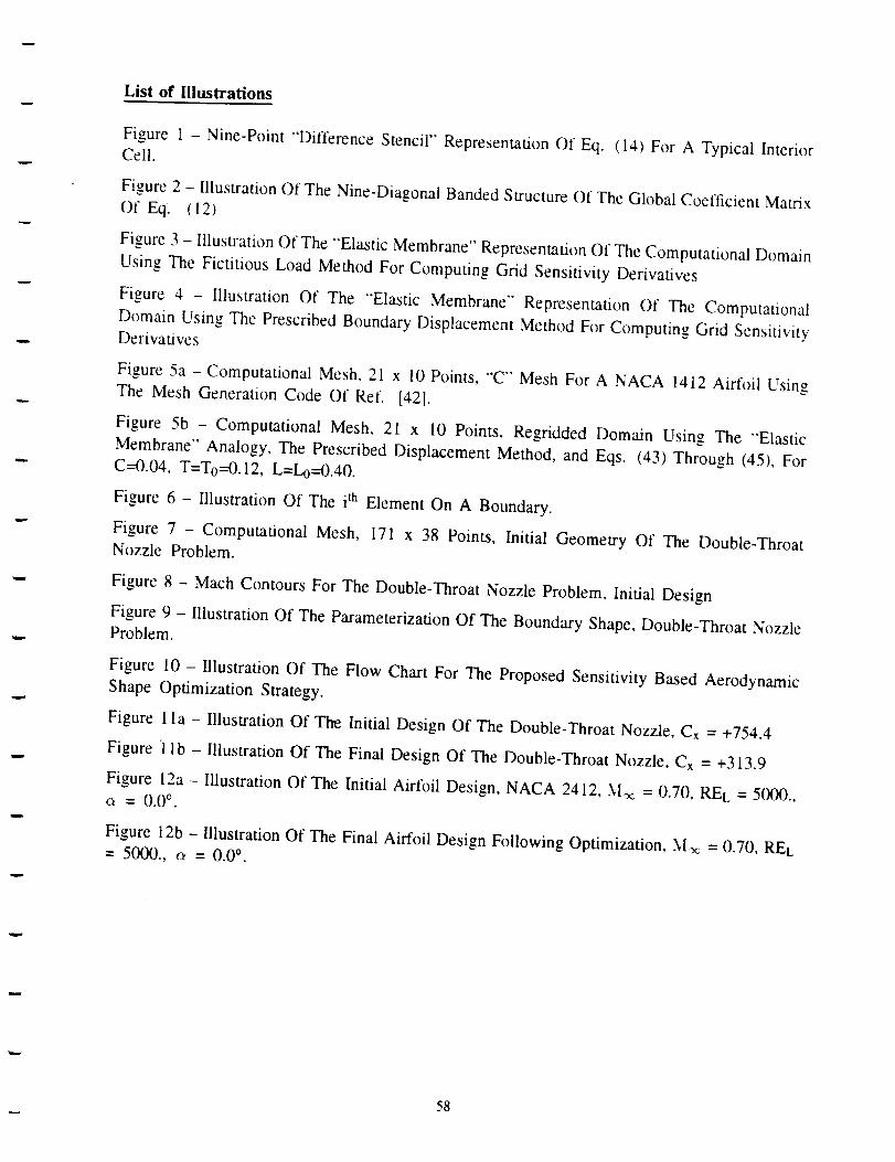
List of Illustrations

Figure I - Nine-Point "Difference Stencil" Representation Of Eq. (14) For A Typical Interior

Cell.

Figure 2 - Illustration Of The Nine-Diagonal Banded Structure Of The Global Coefficient Matrix

Of Eq. (12)

Figure 3 - Illustration Of The "Elastic Membrane" Representation Of The Computational Domain

Using The Fictitious Load Method For Computing Grid Sensitivity Derivatives

Figure 4 - Illustration Of The "Elastic Membrane" Representation Of The Computational

Domain Using The Prescribed Boundary Displacement Method For Computing Grid Sensitivity

Derivatives

Figure 5a - Computational Mesh, 21 x 10 Points, "C'" Mesh For A NACA 1412 Airfoil Using

The Mesh Generation Code Of Ref. [42].

Figure 5b - Computational Mesh. 21 x 10 Points, Regridded Domain Using The "'Elastic

Membrane" Analogy, The Prescribed Displacement Method, and Eqs. (43) Through (45), For

C---0.04, T=To--O. 12, L=L0--0.40.

Figure 6 - Illustration Of The i th Element On A Boundary.

Figure 7 - Computational Mesh, 171 x 38 Points, Initial Geometry Of The Double-Throat

Nozzle Problem.

Figure 8 - Mach Contours For The Double-Throat Nozzle Problem, Initial Design

Figure 9 - Illustration Of The Parameterization Of The Boundary Shape, Double-Throat Nozzle

Problem.

Figure lO - Illustration Of The Flow Chart For The Proposed Sensitivity Based Aerodynamic

Shape Optimization Strategy.

Figure 1 la - Illustration Of The Initial Design Of The Double-Throat Nozzle, Cx = +754.4

Figure 1 lb - Illustration Of The Final Design Of The Double-Throat Nozzle, Cx = +313.9

Figure 12a- Illustration Of The Initial Airfoil Design, NACA 2412, Moc = 0.70, REL = 5000,

o = 0.0 °.

Figure 12b - Illustration Of The Final Airfoil Design Following Optimization, _I_ = 0.70, REL

= 5000., c_ = 0.0 °.

58

,C-H -

--i-- OBO

-G-)

k÷2

k÷l

• ) k

k-I

k-2

-2 j-_ j j,_ j,2

Fig. (])- Nine-Poim "Difference Stencil"

Representation Of ,_I. (14) For A Typical Interior Cell.

D,A,B,C,E

nAQ = Rn(Q,

Fig. (2) - Illustration Of The Nine-Diagonal Banded

Structure Of The Global Coefficient Matrix Of Eq. (12)

Unit

I

r

Symbol Indicates Simple Support, Zero Displacement.

(Points Supported Included Leading And Trailing Edges,

Points In Wake, And All Points At The Far-Field Boundary)

Fig. (3) - Illustration Of The "Elastic Membrane" Representation Of The Computational

Domain, Using The Fictitious Load Method For Computing Grid Sensitivity Derivatives.

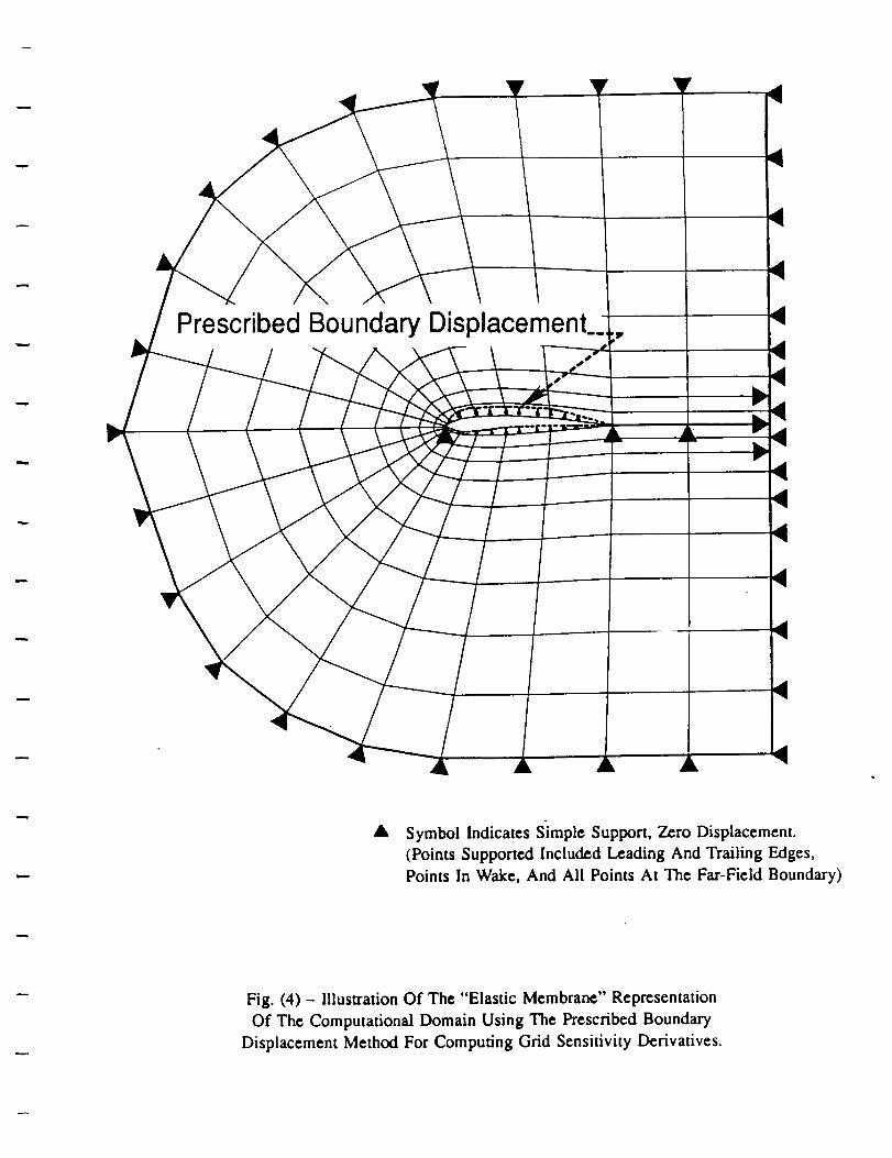
Prescribed Boundary Displacement._.

kB

/

Symbol Indicates Simple Support, Zero Displacement.

(Points Supported Included Leading And Trailing Edges,

Points In Wake, And All Points At The Far-Field Boundary)

Fig. (4) - Illustration Of The "Elastic Membrane" Representation

Of The Computational Domain Using The Prescribed Boundary

Displacement Method For Computing Grid Sensitivity Derivatives.

0 _ LI

_.)

._._°_[-, it

× 0

0 e"

ONo-.

,-_=

_o

_._0

x_

0

v

Z

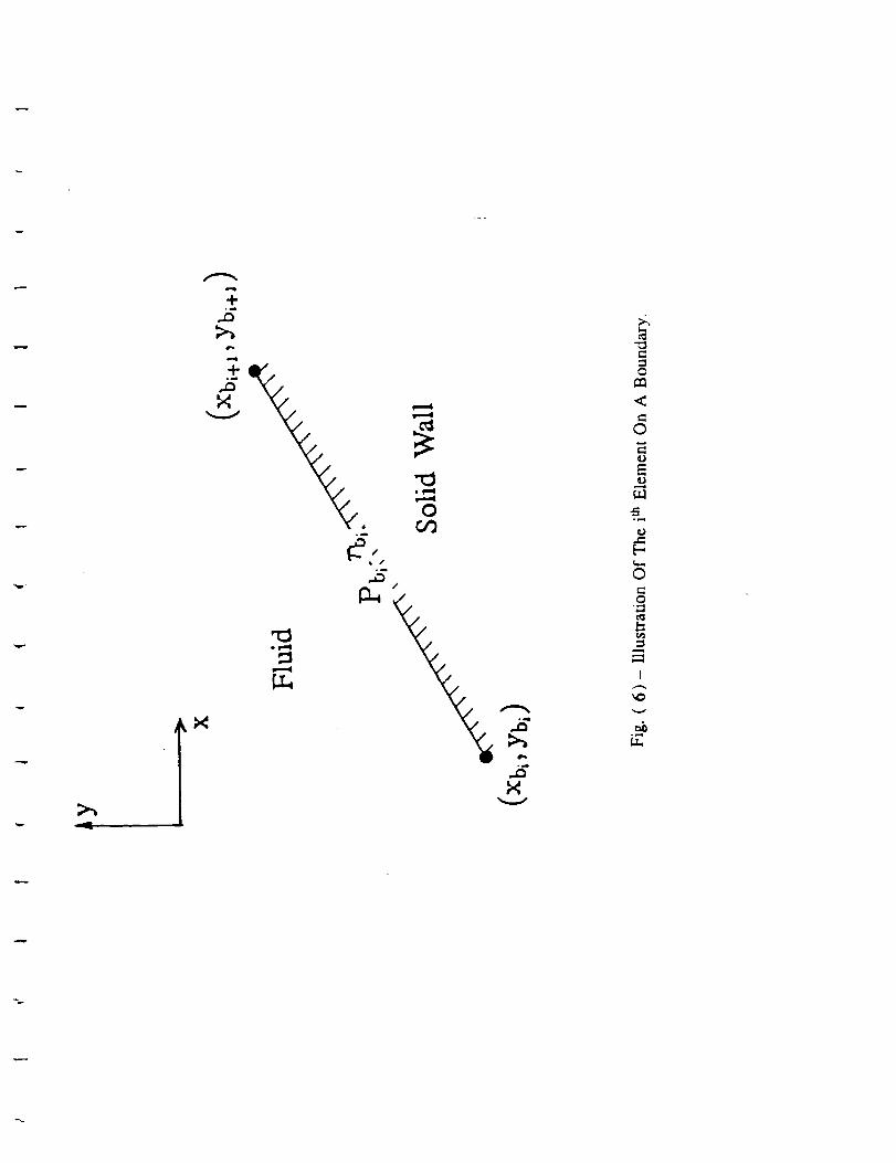
qpv.11

w_

X

f.,MiO

©

q_

o_

©

0

c_

r_

pm_

I

°,mr

L_

Ott3

O

O-12.00

T T R r T T

-5.50 -2.25 1. O0 _. 25 7.50 tO. 75

X AXIS

Fig. (71 - Computational Mesh, 171 x38 Points, Initial

Geometry of The Double-Throat Nozzle Problem.

Fig. (8) - Mach Contours For The Double-Throat Nozzle Problem, Initial Design.

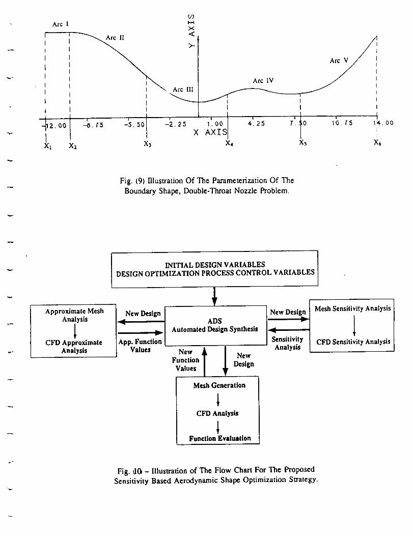
Arc 1

[ II

III

II

I

I

I

i

2. O01 X2

'_, r5 , 50i

X3

c.,oi..,-ix<

Arc III

>.

Arc V /

Arc IV

I

I I I _ I

a

1.00 ¢.25 T.10 10. /'5AXIS

X4 Xs

1 I.. O0

X6

Fig. (9) Illustration Of The Parameterization Of The

Boundary Shape, Double-Throat Nozzle Problem.

Approximate MeshAnalysis

lCFD Approximate

Analysis

INITIAL DESIGN VARIABLESDESIGN OPTIMIZATION PROCESS CONTROL VARIABLES

New Design ] New Design

ADS II_ Automated Design Synthesis __

App. Function SensitivityValues Analysis

New T _ Des

Function NewValues ign

Mesh Generation

CFD Analysis

Function Evaluation

Mesh Sensitivity Analysis

1CFD Sensitivity Analysis

Fig. dO - Illustration of The Flow Chart For The Proposed

Sensitivity Based Aerodynamic Shape Optimization Strategy.

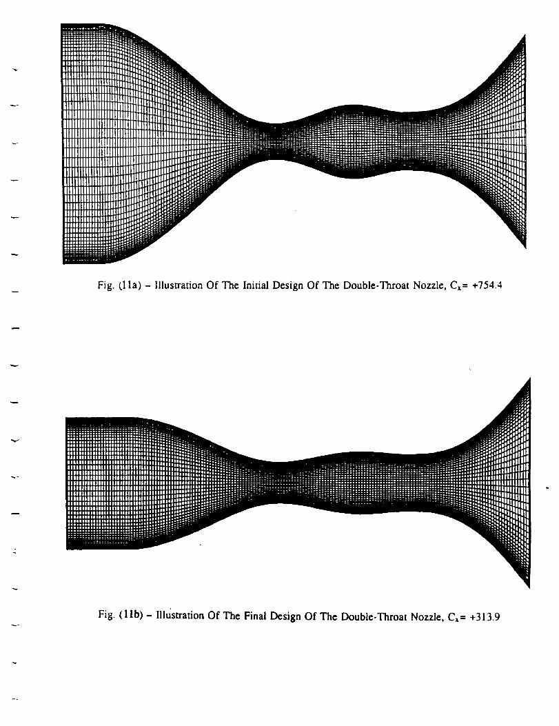
Fig. ¢.1la) - Illustration Of The Initial Design Of The Double-Throat Nozzle, Cx= +754.4

Fig. (I lb) - Illustration Of The Final Design Of The Double-Throat Nozzle, Cx= +313.9

Fig. (12al - Illustration Of The Initial Airfoil Design,

NACA 2412, Moo = 0.70, REL=5000, a--0.0 °

Fig. (12b) - Illustration Of The Final Airfoil Design

Following Optimization, Moo =0.70, REL=5000, a=0.0 °