rii'D.:::::'W':----------,r::;---:::"----:----:----::-:---~----T CENTER FOR LIBRARY L E P AG E 1. R..-rt Na. 2. Go"•'""'"' Acca .. ian No. 3 11111111111 h~~~~~lm'jl~' ~ FHWA/TX-90+1129-2F ~1111 1111 I

4. Title and Subtitle

ANALYSIS AND DESIGN OF BRIDGE BENT COLUMNS

7. Authorial

M. Haque, J. M. Roesset, and C. P. Johnson

9. Performing Organiaotion N-e and Addra ..

Center for Transportation Research The University of Texas at Austin Austin, Texas 78712-1075

5. Report Date

November 1988 6. Perfonning Organi ration Code

B. Parfor111ing Orgoni ration Report No.

Research Report 1129-2F

10. Worlo Unit No.

I 1. Contract or Grant No.

Research Study 3-5-86-1129

r.~-:----------..,....,....----------------.....113. Type of Report and Period Covarad 12. Sp..,aoring Agency N-• ..,d Addrau

Texas State Department of Highways and Public Transportation; Transportation Planning Division

P. 0. Box 5051 Austin, Texas 78763-5051 15. Suppla,._tary Natea

Final

14. Sponaaring Agency Coda

Study conducted in cooperation with the U. S. Department of Transportation, Federal Highway Administration

Research Study Title: "Bent Column Analysis and Design" 1~176.~A71o~.,~ •• ~c~t---------------------------------------~

I

The behavior of bridge bents under spatial loads was investigated to evaluate the suitability of the current office procedure of the Texas State Department of Highways and Public Transportation (TSDHPT) for analyzing and designing slender concrete bridge bent columns. Two computer codes were developed for this purpose.

The linear method of analysis uses the conventional direct stiffness method of solution and considers linear material behavior. The AASHTO moment magnifier method was used to approximate second order effects. The design forces from the linear analysis were compared with those from the TSDHPI' approximate procedure. The effect of variation in live load positions over the bridge deck was examined.

The nonlinear method of analysis, developed in this study, uses a fiber model and an updated Lagrange finite element formulation to predict the space behavior of multistory concrete bents. The analytical results for typical bents were compared with those from the TSDHPT approximate method and the AASHTO moment magnification procedure. The sensitivity of the results to bent column slenderness and foundation flexibilities were examined in terms of predicted bent behavior.

17. Kay Warda

bridge bent, column, behavior, inplane, out of plane, loads, procedures, analysis, design, linear moment mag­nifer method, three-dimensional

11. Dlotrlllutl• St•--•

No restrictions. This document is available to the public through the National Technical Information Service, Springfield, Virginia 22161.

19. S.curtty Cla .. lf. (of thio ~J

Unclassified

Z. Sowrity Clo .. lf. (of thla , ... ,

Unclassified

21. No. of Pogo• 22. Price

76

Fo1111 DOT f 1700.7 ,, ... ,

ANALYSIS AND DESIGN OF BRIDGE BENT COLUMNS

by

M. Haque J. M. Roesset C. P. Johnson

Research Report Number 1129-2F

Research Project 3-5-86-1129

Bent Column Analysis and Design

conducted for

Texas State Department of Highways and Public Transportation

in cooperation with the

U.S. Department of Transportation Federal Highway Administration

by the

CENTER FOR TRANSPORTATION RESEARCH

Bureau of Engineering Research

THE UNIVERSITY OF TEXAS AT AUSTIN

November 1988

The contents of this report reflect the views of the authors, who are responsible for the facts and the accuracy of the data presented herein. The contents do not necessarily reflect the official views or policies of the Federal Highway Administration. This report does not constitute a standard, specification, or regulation.

ii

There was no invention or discovery conceived or first actually reduced to practice in the course of or under this contract, including any art, method, process, machine, manufacture, design or composition of matter, or any new and useful improvement thereof, or any variety of plant which is or may be patentable under the patent laws of the United States of America or any foreign country.

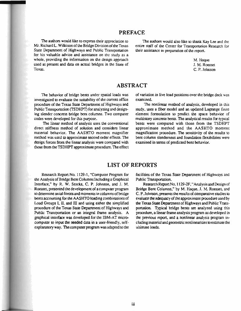
PREFACE

The authors would like to express their appreciation to Mr. Richard L. Wilkison of the Bridge Division of the Texas State Deparunent of Highways and Public Transportation for his valuable advice and assistance on the study as a whole, providing the infonnation on the design approach used at present and data on actual bridges in the State of Texas.

The authors would also like to thank Kay Lee and the entire staff of the Center for Transportation Research for their assistance in preparation of the report.

M. Haque J. M. Roesset C. P. Johnson

ABSTRACT

The behavior of bridge bents under spatial loads was investigated to evaluate the suitability of the current office procedure of the Texas State Department of Highways and Public Transportation (TSDHP1) for analyzing and design­ing slender concrete bridge bent columns. Two computer codes were developed for this purpose.

The linear method of analysis uses the conventional direct stiffness method of solution and considers linear material behavior. The AASHTO moment magnifier method was used to approximate second order effects. The design forces from the linear analysis were compared with those from the TSDHPT approximate procedure. The effect

of variation in live load positions over the bridge deck was examined.

The nonlinear method of analysis, developed in this study, uses a fiber model and an updated Lagrange finite element formulation to predict the space behavior of multistory concrete bents. The analytical results for typical bents were compared with those from the TSDHPT approximate method and the AASHTO moment magnification procedure. The sensitivity of the results to bent column slenderness and foundation flexibilities were examined in tenns of predicted bent behavior.

LIST OF REPORTS

Research Report No. 1129-1, "Computer Program for the Analysis of Bridge Bent Columns Including a Graphical Interface," by R. W. Stocks, C. P. Johnson, and J. M. Roesset, presented the development of a computer program to determine axial forces and moments in columns of bridge bents accounting for the AASHTO loading combinations of Load Groups I, II, and m and using either the simplified procedure of the Texas State Department of Highways and Public Transportation or an integral frame analysis. A graphical interface was developed for the IBM-AT micro­computer to input the needed data in a user-friendly, self­explanatory way. The computer program was adapted to the

1U

facilities of the Texas State Deparunent of Highways and Public Transportation.

ResearchReportNo.1129-2F, "Analysis and Design of Bridge Bent Columns," by M. Haque, J. M. Roesset, and C. P. Johnson, presents the results of comparative studies to evaluate the adequacy of the approximate procedure used by the Texas State Department of Highways and Public Trans· portation. Typical bridge bents are analyzed using this procedure, a linear frame analysis program as developed in the previous report, and a nonlinear analysis program in· eluding material and geometric nonlinearities to estimate the ultimate loads.

SUMMARY The Texas State Department of Highways and Public

Transportation uses at present an approximate procedure for the analysis and design of the columns of a bridge bent In this procedure axial loads due to gravity are uniformly dis­tributed among the columns, the moments due to inplane lateral loads are computed assuming an inflection point at the midheight of the columns, and the moments due to out of plane loads are estimated assuming each column as a canti­lever. The column lengths are increased to take into account the flexibility of the foundation including a depth to fLXity which is based on engineering judgment and experience. Finally, slenderness or second order geometric effects are considered using a k factor of 1.25.

The purpose of the present study was to assess the validity of these approximations. For this purpose a series of typical bridge bents were considered and analyzed using a linear frame analysis with the k factors suggested by AASIITO and a true nonlinear analysis which incorporates material and geometric nonlinearities to estimate the ulti­mate loads. In the linear analysis the effect of varying the position of the truck loads over the bridge deck was also investigated. It should be noticed that although a frame analysis is theoretically correct, itassumesrigidjoints which may not really exist due the available size for development

length of the rebars. Thus the present approximate proce­dure, while a simplification, is also based on imponant practical considerations.

A series of comparative studies have been conducted using both the linear and the nonlinear analysis procedures and the present approximations. The results of these sUJdies indicate that for bents where the girders are symmetrically arranged and for slenderness ratios less than 40 (ratio of the column length to the radius of gyration of the cross section) the approximate procedure yields very reasonable results. When the girders are arranged in a highly unsymmetrical pattern the axial forces in the columns assuming a uniform distribution may be underestimated. particularly if the live loads are moved along the width of the deck. For columns with slenderness ratios larger than 60 some care must be exercised: the ultimate loads may be substantially smaller than those obtained from the nonlinear analyses. Ultimate loads computed using the AASIITO procedure tend to be, on the other hand, conservative and excessively so for very slender frames.

The results indicate also that the useofthedepth to fLXity to account for the foundation flexibility seems to provide reasonable and conservative results for the range of soil properties considered in the analyses.

IMPLEMENTATION STATEMENT

Comparison between the results obtained using linear and nonlinear frame analysis programs and the approximate procedure used at present by the Texas State Departtnent of Highways and Public Transportation indicates that this procedure gives reasonable design forces for bents with a nearly symmetric arrangement of the girders over the bent cap and for slenderness ratios of the order of 40 or less. The

iv

use of a depth to fixity, based on engineering judgment, to account for the foundation flexibility provided also a rea­sonably conservative solution for the cases considered.

Some care must be exercised, however, when the pro­cedure is applied to bents with unsymmetric arrangement of the girders, and in particular when dealing with slenderness ratios larger than 60.

TABLE OF CONTENTS

PREFACE-----·----------------------------------·-·--·--------······---·---·-.................................. iii

ABSTRACf --------------··-----------·--·---------·-·---·--·---··------·---·-·.......................................... iii

LIST OF REPORTS ·-·-----·----------·------------·--·····---·--·--·-----·····....................................................... iii

~Y.................................................................................................................................................................................................................. iv

l1v1PI..EMENT A TI()N' STATEMENT................................................................................................................................................................. I v

CH~l.ThiTRODUCfiON

1.1 General.................................................................................................................................................................................................... 1 12 ()bjectives............................................................................................................................................................................................... 3

1.3 Outline of Contents·-·---·-----·----......................... -...................................................................................................... 3

CHAPTER 2. ANALYSIS PROCEDURES 2.1 General Consideration·-------·--·------------·--·-----··-·--.................................................................... 4

2.1.1 Loading Combinations ........ ----·---------·--·--------·-·--·-·-···-...................................................... 4 2.12 MOillelll Magnifiel' Method.............................................................................................................................................. 4

22 Approxinlale Procedure.................................................................................................................................................................... 5

2.3 Linear Analysis of Bents---------------------------·--·-·-................................................................. 5 2.4 Nonlinear Analysis of Bents .... --------·-------·----·------·-···.................................................................. 6

C~ 3. NONLINEAR ANALYSIS FORMULATION

3.1 Introduction----------·-------·-----------------·--------··-........................................................ 8 32 Derivation of the Stiffness Mattix............................................................................................................................................... 8 3.3 Geometric Nonlinearity.................................................................................................................................................................... 12

3.4 Malerial ~ly ........................................................................................................................................................................ 13

3.5 Solution Procedure-----------------------------·----·---.............................................................. 15 3.5.1 Computation of Element Distortions .... -------·---·---·---·---·--·-·--............................................. 15 3.52 Iterative Solution·---------------------·-----·--·--·-·--·--·-................................................... 15

CHAPTER 4. VALIDATION OF COMPUTER PROGRAM

4.1 Introduction ..... ----------------------·------·---... -................................................................................ 17 42 Effect of Number of Segments Per Member .......................................................................................................................... 17 4.3 Effect of the Size of Load Steps.................................................................................................................................................. 17

4.4 Comparison with Analytical Results .. -----------------·--·--·-·--·--............. - ..................................... 19 4.5 Comparison with Experimental Results··----·-----------·-----------·----................................... 19 4.6 Summary·---------------------------------------------·---·---..................................... 20

CHAPTER 5. RESULTS AND DISCUSSION

5.1 Introduction--------------------------------·-----···--·--·-· ........................................................ 23 52 Bent Configuration----------------------------------·---·--..................................................... 23 5.3 Loads 00 Bents. .................................................................................................................................................................................... 23

5.4 Approximate Procedure Vs Linear Frame Analysis-------------·---·-·-·---·-· ........................................ 23

5.4.1 Group I Loads-----------------·--------------------·----........................................... 23 5.42 Group n Loads.. ....................................................................................................................................................................... 24

v

5.43 Group ill Loads-------------·---------·-------·--···--···-·---···········-·-·················-··············· 24 5.4.4 I>iscussKxl of Results. ... - ... ·-·--·-·-·-·-·-·--·-·-·-····-·-·--·-·-····-·-·--·-····-····-·····················-·-··················-···-········· 24

55 Approxiinate Procedure Vs Nonlinear Analysis·------·---·-·--·-···---·-···················-························-················ 34

55.1 Load-[)efoonali<x:l Curves.·-·-·-·-·-·-·-·-·-·-·-·-·-·-·-·-·-·-·--·-·-·-·-·-·-·-·-·-·-····-·-····-····-·-·········-····-····-......... 34 55.2 Predicted Axial Loads Vs Design Axial Forces--·----·--··-----··--··--··-··········-········--·-··-·-··-·-... 34 553 PrOO.icted Motnents Vs Design Moments ................................................................................................................... 34

55.4 Effect of Slenderness Ratio of Bent Columns--·---·--------·-·-·-.... --........ _ ................. - ................ 50 555 Effect of Foundation Aexibility ·-----.. -------·--·--·-------··· .. --..................................................... 53

5.6 S urn mary·---------------------·-·----·------·------··--.. ·-·-·-.... -..... -........................................... 54

CHAPTER 6. CONCLUSIONS AND RECOMMENDATIONS

6.1 Summary of the Study·---·-----------.. ---·---·-------·---·-·--.......................... -..................................... 66 6.2 Approximate Procedure Vs Nonlinear Analysis·---·--------·-·--·---·-............................................................ 66

6.1.1 ApJxoxiinale Procedure V s Linear Frame Analysis.......................................................................................... .... 66 6.1.2 Approxilnale Procedure V s Nonlinear Analysis....................................................................................... ............... 66

63 Research Needs-·------------·--·-----·-·---·--............................................... - .................................................. 67

REFERENCES--------------------------------·--.. ------·--------··· ........................................................................................... 68

vi

CHAPTER 1. INTRODUCTION

1.1 GENERAL The design of bridge bent columns requires the determi­

nation of axial forces and associated moments. The design loads necessary for analyzing bent columns are provided in the American Association of State Highway and Transpor­tation Officials (AASHTO) Specifications [4]. There are twelve loading combinations specified by AASHTO which must be considered in computing the design loads. Of these twelve loading combinations, three groups govern the de­sign of columns for typical Texas highway bridge bents. Figures 1.1 and 1.2 on the following page show a typical highway multi-column bridge bent. The design loads in­clude dead load, live load, impact, earth pressure, buoyancy, wind load on structure, wind load on live load, longitudinal force from live load, centrifugal force, rib shonening, shrinkage, temperature, earthquake, stream flow pressure, and ice pressure.

1.1.1 Cun-tnl Texas Highway Departnunt Approach

The Texas State Deparunent of Highways and Public Transportation (TSDHP'I) has identified AASHTO load groups I, II and Ill as the critical loading combinations for designing bridge bents. The current office procedure of analysis involves utilizing an approximate method derived for hand analysis. Since the bent cap and column system is an indeterminate frame, simplifying assumptions are made in order to make hand analysis possible. The column mo­ments, due to in-plane lateral loads, are computed assuming an inflection point located at the mid-height of all columns. This assumption may or may not be reasonable depending on the relative stiffness between the bent cap and the columns. Another drawback in the approximate method is that changes in axial loads due to horizontal forces are not taken into account. Neglecting the effect of overturning forces on the axial forces results in final design loads which are not conservative in all cases. A final simplifying assumption is that all columns receive an equal percentage of the total load on the bridge. Although the loads from the superstructure are transferred to bent columns via the girders, the location of these beams over the bent cap is not included in the approxi­mate procedure. No consideration is given for the variation in the live load positions over the bridge deck.

The moments computed for the latelalloads are ampli­fied to include second order effects. There have been several methods advocated for the analysis of compression mem­bers [17,18,32,33]. The approximate method of the TSDHPT uses the moment magnifier method of AASHTO [4] to approximate the slenderness effects. The AASHTO provisions are based on the ACI Building Code [ 1 ,2] which focuses on strength and do not clearly focus on lateral displacements, although such deflections are implicitly

included in the moment magnification procedure. The ex­tensive experimental and analytical studies [2,6,18] which formed the basis for the code provisions considered typical columns and loading conditions fowtd in buildings. Most buildings have small story drifts, thus lateral deflection is not a primary concern. In bridge bent design, the lateral dis­placements are considerably higher and therefore lateral deflection may be an imponant factor. The AASHTO provi­sions do not explicitly alert designers when deflection might be a problem.

An important aspect of the moment magnification pro­cedure lies in the evaluation of the effective length factor (k) and the reduced column stiffness due to nonlinear effects. The code provides empirical equations for estimating the reduced stiffness of columns and beams. The difficulties in using the effective length approach are associated with the evaluation of the restraints at the column ends. In most Texas highway bridges, little or no restraints are provided at the top of the bent especially in the direction parallel to the bridge axis. Also, the base of the columns are far from fuity. ln these conditions, the effective length factor (k) may vary from 1.5 to 3.0 [25]. The degree of fixity at the foundation level is an extremely significant parameter affecting the k values. There is no guidance given in AASHTO on how to evaluate it. The evaluation of rotational and translational restraints for various fowtdation conditions requires a great deal of judgemenL The problem of soil-structure interaction has been addressed by several authors [5,20,22,26,31] for both shallow and pile foundations, wtder both static and dynamic loadings. The results have been presented in tenns of equivalent spring stiffnesses which depend on the soil properties (shear wave velocity) and the type and size of the foundation. The determination of the shear wave velocity is a formidable task. Empirical equations relating the shear wave velocity and number of blow counts have been pre­sented in the literarure [28,30].

In the event of uncertainty in the foundation fuity, the current office procedure assumes an increased column length and a fixed base to simulate the soil-structure interac­tion effects. The increased column length is called " Depth to fiXity" (Fig 1.2). Its value ranges from 4 to 10 feet depend­ing on the soil conditions and the engineer's judgment.

With the faxed base, the bent behaves like a cantilever in the out of plane direction and as an unbraced frame under in-plane loads. For this case, the code provisions recom­mend the useofk values of2.0 for the out of plane bending. The effective length factor for in-plane behavior should be computed considering the interaction of rotational restraint of beams on columns. The approximate procedure of the TSDHPT assumes an effective length factor of 1.25 for both axes ofbending. The value is used irrespective of there lati ve

2

1+--- Bent Column

Fig 1.1. Bridge bent.

It I

Rail

Bent Cap

Bent Column

Watar Une

Ground Depth to

Fixity Assumed Foclty

Fig 1.2. Bent column elevation.

sizes of beams and columns, the loading conditions, and the column slenderness. The moment magnification procedure of analysis was originally developed for uniaxial bending. The procedure is greatly complicated when biaxial bending is considered. The ACI Code [1,2] conservatively recom­mends to amplify the moments about both axes, computed from a linear analysis, independently of their associated moment magnification factors. The present code provisions do not account for the interaction between the two axes of bending. The TSDHPT approximate procedure essentially uses the code method to approximate the biaxial slenderness effects.

1.2 OBJECTIVES The purpose of this investigation was to study the

suitability of the current office procedure of the TSDHPT in predicting the design forces and the behavior of slender bents. The study involved developing two computer pro­grams for the analysis of reinforced concrete bridge bents.

The linear frame analysis program utilizes the direct stiffness method of solution and considers linear material behavior. The moment magnifier method of the code is used to approximate second order effects. The program was used to compute the design forces for bent columns.

The nonlinear analysis program was developed to ana­lyze reinforced concrete bridge bents under spatial loads. The fiber model [3,23] and an updated Lagrange fmite element formulation were used to model the geometric and material nonlinearities. The program was used to predict the behavior of typical bents up to failure.

The primary objectives of this study were: (I) To compare the design loads obtained from the ap­

proximate method with those obtained using the linear frame analysis.

3

(2) To investigate thesensitivityofvariations in the live load positions, over the bridge deck, on the computed design forces from the approximate procedure.

(3) To compare the moments obtained from the ap­proximate procedure and the AASI-ITO moment magnifier method with those obtained from the nonlinear analysis.

( 4) To investigate the effect of column slenderness ratio on the behavior of bents and to evaluate the sensitivity of foundation flexibilities, comparing the results for various foundation conditions with the current approach of the approximate procedure.

1.3 OUTLINE OF CONTENTS Chapter2 describes the analysis procedures used in this

study. Computation of various loads on bridges are briefly discussed. A brief review of the AASHTO momem magni­fier method is presented.

Chapter 3 presents a detailed derivation of the equations for the nonlinear analysis. The solution procedure and con­sideration of geometric and material nonlinearities are de­scribed.

In Chapter 4, the accuracy and efficieocy of the nonlin­ear analysis program are verified. The predictions of the pro­gram are checked against experimental results and other analytical predictions.

Chapter 5 contains the comparison between the design forces obtained from the linear frame analysis and the approximate procedure. The results of nonlinear analyses are compared with those obtained from the ACI moment magnifier method and the TSDHPT approximate procedure. The effects of column slenderness and foundation flexibili ry on the bent behavior are iocluded in this chapter.

Chapter 6 summarizes the conclusions and recommen­dations for fwther research.

CHAPTER 2. ANALYSIS PROCEDURES

2.1 GENERAL CONSIDERATION The Texas State Department of Highways and Public

Transponation (TSDHPT) uses an approximate procedure, suitable for hand calculations, to compute the design axial forces and associated bending moments in bridge bent columns. The approximate procedure assumes that the col­umn moments are developed due to lateral loads and the axial forces in columns are induced by gravity loads only. The contribution of the lateral loads on the axial forces and that of the gravity loads on the bending moments are ne­glected. In the linear and nonlinear analyses used in this study, the bent cap and the columns are treated as an integral frame. The gravity loads are equally divided between the girders. Thus moments and axial forces in columns are developed due to both the gravity and lateral loads. To compute the design forces and moments for a particular structure, the bridge must be defmed by several variables including bridge geometry, geographic location, and prop­erties of the construction materials.

2.1.1 Loading CombiiUJtions

The design of bent columns requires determining the critical axial loads and bending moments considering twelve loading combinations following AASHTO specifications. Of these twelve loading combinations or groups, TSDHPT has identified groups I, II and ill as the critical loading combinations which must be considered in the design of typical Texas highway bridge bents. These loading combi­nations are

Group I = 1.30*[f~ItDL+1.67•(LL+I)+CF+SF] Group II = 1.30* [~0 •DL+SF+ W] Group III = 1.30•[~0 •DL+(ll.+I)+CF+SF+0.3•W

+WL+LF]

The dead load (DL) computations include the weights of bridge rails, slab, beams, bent cap and the columns. The variable ~is the load combination coeffiCient for the dead load. A value ofO. 75 is assigned when checking a column for the minimum axial load and maximum moment or maxi­mum eccentricity. A value of 1.0 is used when checking a column for the maximum axial load and minimum moment The live loads (LL) as specified by AASHTO include lane load and truck load. The larger of the two live load values is used in computing the live load plus impact(ll.+l). The live load intensity is reduced according to AASHTO Article 3.12 for a multiple lane bridge in view of the improbability of coincident maximum loading. For one or two lanes, no reduction is allowed. For three lanes, the reduction factor is 0.90.Forfourormorelanes,thereductionfactoris0.75. The value of CF represents the centrifugal force associated with curved bridges. The value of SF represents the stream flow for columns subjected to design water pressure. The wind load (W) includes the effect of wind pressures on the bridge

4

superstructure, specified in AASHTO Article 3.15 .2.1.1, as well as wind forces applied directly to the bridge substruc­ture, specified in AASHTO Article 3.15.2.2. AASIITO recommends the use of five wind directions, relative to the longitudinal axis of the bridge, in com puling the wind forces on the bridge. The design wind forces provided by AAS liTO are derived on a base wind velocity of 100 miles per hour. According to AASHTO Article 3.15, the design wind forces for load group II must be reduced or increased by the ratio of the square of the design wind velocity to the square of the base velocity. The values of WL represent wind load on moving live loads, specified in AASHTO Article 3.15 .2.1.2. The longitudinal force (LF) represents the effect of the acceleration or deceleration of vehicles, and it is taken as a percentage (5%) of the live load. specified in AASHTO Article 3.9.

The column's axial load and associated bending mo­ments are computed for each load group. The moments are compared with the minimum eccentricity moments to en­sure that the critical values are used in design. The factored moments are then amplified to include second order effects, commonly called P~ effects. There have been several meth­ods of analysis advocated for slender compression members. These include the Reduction Factor Method, the Stability Index Procedure, the Moment Magnifier Method and com­puter based second order frame analysis. An excellent re­view of these procedures is given elsewhere [25]. The TSDHPT uses the ACI Moment Magnifier Method to ap­proximate the second order effects in columns. The method has been adopted by AASHTO as a basic approximate procedure for determining slenderness effects in concrete compression members. The moment magnification proce­dure of the ACI code is briefly described in the next subsec­tion.

2.1.2 MotMnl Magni.fur Method

The ACI Building Code recommends the use of this method to approximate the effect of column slenderness and other nonlinearities on the column forces and moments. The code procedure is based on the evaluation of an effective length factor and a moment magnifier. The moments com­puted using an elastic frame analysis and linear force­deformation relationships are multiplied by a coefficient, called the moment magnification factor. The magnification factor is a function of the applied axial load, the column critical buckling load, the ratio of column end moments, and the column deflected shape. For unbraced frames, the code recommends the use of the following expression for comput­ing design moments.

M = SbM + S M (2.1) c I I I

where

ob = moment magnification factor for frames braced against sidesway

o = sway moment magnification factor I

M = equivalent design moment c M = moments due to gravity load (nonsway

8 moments) M = lateral load moments (sway moments)

I

For frames braced against sidesway, Equation (2.1) is used with sway moments as zero. The moments M and M are computed using an elastic frame analysis w~ere the

1

un­cracked section properties of the members are used for the stiffness calculation. The moment magnifiers ob and 0

1 are

ob = Cm I (1 - (P j~P .)) ~ 1.0

and

01

= 11 (1 - (D> j~LP .)) ~ 1.0

in which

where

P = ,rEI I (kL i c u

P = axial load in the column ~

P< = critical or Euler buckling load of colwnns ~ = capacity reduction factor em = an equivalent moment correction factor

= 0.6 + 0.4 [Ml~] (0.4 ~ CID ~ 1.0) M 1 and ~ = smaller and larger column end

moments respectively, detennined from the first order analysis

k = effective length factor EI = stiffness of the column L = unsupported length of the colwnns.

u

The stiffness of the column and the restraining members are the major parameters and as a consequence the accuracy of the magnification factor is highly dependent on the values used. The effective EI of reinforced concrete depends on the magnitude and the type of loading, and the variation of material properties along the column length. The code recommends the following fonnuJas for the effective EI rex­reinforced concrete compression members.

where

EI = 0.4 E I c I

for p S 2%

EI = 0.2E I + E I for p > 2% c I I •

E = elastic modulus of concrete c E = elastic modulus of reinforcement •

(2.2)

(2.3)

I = moment of inertia of gross concrete section, 1 neglecting reinforcement

I = moment of inertia of reinforcement about 1

centroidal axis of member cross section p = reinforcement ratio.

s

The maximwn of the above two values of EI are used in computing the column critical buckling load The effect of sustained load is included by dividing Equations (2.2) and (2.3) by (l+Bd), where Sdis the ratio of the maximum design dead load moment to the maximwn design total load mo­ment The effective length factor is computed using align­ment charts [2].

The following sections include a description of the approximate and the frame analysis procedures.

2.2 APPROXIMATE PROCEDURE The ftrst step in the TSDHPT analysis procedure is to

detennine the Euler buckling load of the column needed for computing the ACI moment magnifier. This computation requires the selection of an appropriate effective length factor as defmed in AASHTO Article 8.16.5.2.3 [4]. The TSDHPT uses a k-factor of 1.25 for both x-axis (in-plane) and z-axis (out of plane) bending for typical bridge benl columns.

Next, the dead and live loads of the structure are computed. The gravity loads on the strucnrre are divided equally between the columns. The columns are isolated for computing the bending moments. The column moments due to in-plane lateral loads (in-plane moments) are computed by assuming the inflection point at the mid-height of the column. Conservatively, the moments due to out of plane lateral loads (out of plane moments) are computed using the total height of the column. AASHTO has specified the locations at which the lateral forces are applied in computing these moments. The axial loads and moments computed for various forces are combined in accordance with AASHTO load groups I, II and m. The details of the computer code for computation of these loads for a typical bridge bent are given by Stocks [29]. The design bending moments about both axes are computed by magnifying the lateral load moments as

M =oM c •

where

o = 11 (1 - (P j~P .))

It may be noted that the magnification factors o and o, are the same for a bent with identical columns since the mo­ments due to gravity loads are neglected in the approximate procedure.

2.3 LINEAR ANALYSIS OF BENTS In the linear analysis, the bent cap and the columns are

treated as a rigid frame. The linear frame analysis utilizes a six-degree-of-freedom linear beam element to represent each member and uses the conventional direct stiffness method of solution. The standard assumption of small defor­mation, plane sections remaining plane, and true rigid con­nections between members are made. Also, it is assumed that

6

members are originally straight and a linear elastic material following Hooke's law is being used.

As with the approximate analysis, AASHTO load groups I, II and mare utilized in computing the design axial forces and moments. A primary difference between the two analysis procedures is that no assumptions are made con­cerning the location of the inflection points with the integral frame solution. In the frame analysis, the bridge dead load is distributed equally between all the beams and therefore column loads are accurately proportioned. Recall that the approximate procedure distributes the total bridge loads equally between all columns. The live loads on the bridge are approximated in two ways. The first method distributes the total live load on the bridge evenly between the beams. The second approach considers the variable position of the AASHTO live loads over the deck. The position of the truck and lane loads are varied across the width of the deck according to the scheme shown in Fig 2.1. First. one truck or lane load is moved over the entire width of the deck as shown in Fig 2.l(a). Next. each lane of the bridge is loaded with one truck or lane load, and the movement of these live loads is restricted within the AASHTO specified lane width. The loads on the girders are computed assuming the deck slab simply supponed between the girders. For each position oflive loads, the column axial loads and associated bending moments are recorded. The column design forces consist of either the maximum moment and corresponding axial load or the maximum axial load and corresponding bending moment The results obtained with both approaches will be compared.

As mentioned in the discussion of the approximate analysis procedure, AASHTO specifies the location on the bridge structure at which the la1eral forces must be applied. For some load cases, the design lateral forces are applied on or above the superstructure of the bridge. For the frame solution, forces must be applied on the frame itself. Thus, to approximate the AASHTO requirements, the design forces were increased by the ratio of the height specified by AASHTO to the distance between the cap center line and the assumed fixity depth (PD=f"'d i.e. f=PD/d), as shown in Fig 2.2.

The solution provided by the frame analysis yields the axial load and bending moments for each column. These member forces evolve from an elastic analysis, and therefore must be modified by the AASIITO moment magnifier method to approximate second order effects.

2.4 NONLINEAR ANALYSIS OF BENTS The nonlinear analysis procedure also treats the bent

cap and the columns as a rigid frame. In this analysis procedure, the tolal gravity loads on the bridge are divided equally between the beams. The basic formulation selected in this study uses the fiber model and an updated Lagrange formulation. The basic difference between the linear and

nonlinear analyses lies in the consideration of various non­linearities. In the linear analysis procedure, the moment magnifier method is used to approximate the amplification of column moments in order to account for the effect of axial loads on these moments. The nonlinear analysis uses realis­tic moment-curvature relationships based on accurate stress-strain relationships and considers the effect of axial load, variable moment of inertia along the member, and the effect of lateral deflections on moments and forces.

The nonlinear analysis procedure uses a combination of incremental and iterative solutions. For a specified load increment. the iterative solution seeks a configuration which satisfies equilibrium of the structure. The incremental tech­nique is used to fmd the behavior of bents at various loading stages. The loading on the bent is assumed to be static and monotonic. The details of the nonlinear analysis formulation and the solution procedures are described in the next chapter.

Range of Movement

(a) Single truck on the bridge

(b) One truck in each lane

Fig 2.1. Variable position of AASHTO truck.

p

a

:1

L

CHAPTER 3. NONLINEAR ANALYSIS FORMULATION

3.1 INTRODUCTION In this study the updated Lagrangian Finite element

fonnuJation is used to model the behavior of reinforced concrete bridge bents under spatial loads. The approach uses an iterative solution with moving coordinates of the joints. The local axes move with the element and therefore share its rigid body motion. The current defonned state is used as a reference prior to the next incremental step of solution.

The model uses a tangent stiffness fonnulation. For an applied load increment. the incremental displacements are calculated using the conventional stiffness method. Nodal displacements are updated and local axes of each element are established. The distortion of the elements and hence the internal forces corresponding to the nodal degrees of free­dom are computed. The difference between the externally applied loads and the internal forces are the residual forces. If the residual forces are within specified limits then the next step of incremental load is applied and the process is contin­ued either up to the failure of the structure or to a specified load level. If the residual forces do not satisfy the equilib­rium of the structure then the stiffness matrix corresponding to the updated sllains is fanned, incremental displacements are computed and the process is iterated until convergence is achieved. The material and geometric nonlinearities consid­ered in this study are explained later in this chapter.

The analysis procedure assumes that the members are prismatic. A nonprismatic member can be divided into several prismatic members. Each member is then divided into a series of longitudinal segments or elements, and the cross section of the member into longitudinal fibers as shown in Figure 3.1.

3.2 DERIVATION OF THE STIFFNESS MATRIX

The Finite element displacement model is used to arrive at the force displacement relationship for a beam-column element. It is assumed that the effects of shear and torsion on the defonnation are negligible and yielding of the section is a function of the nonnal stress only. The virtual work principle for this case can be stated as

where

L

r&T(60'+<1) dv = jsuT(T+6T) dL vo1.

E = state of nonnal strain in the system

cr = state of nonnal stress in the system

T = applied traction

6cr = increment in nonnal stress

6 T = increment in applied traction

L = length of the element

u = displacement function along the element length

8

The nonnal strain distribution E can be expressed in tenus of axial strain and strains due to bending about two axes. For the local axes of the member shown in Figure 3.2, the nonnal strain distribution in tenns of displacements is

or

E=v·-xu .. -zw .. (3.2)

where prime indicates the derivative of the function with respect toy. In incremental fonn, Equation (3.2) becomes

where

& = tt.v'- x tt.u .. - z tt.w ..

u =displacement in x-direction v = displacement in y-direction w = displacement in z-direction

(3.3)

x = distance of differential element in z-direction z =distance of differential element in x-direction

To evaluate the integrals in Equation (3.l),the element nodal forces and defonnations are chosen as shown in Figure 3.3. It is assumed that the deflected shape of the element about the x and z axes can be expressed as a third degree polynomial. This satisfies the conditions of constant shear and linearly varying bending moment. The shape function in they-direction is assumed to be linear. The deflection at any section along the length of the element can be expressed in tenns of the nodal degrees of freedom as

(3.4)

(3.5)

where g1, ~· f1, f2, f3 and f4 are conventional Hennite inter­polation functions for a beam element. These functions are

X

A

1U9Wf5as

6

10

(a) Forces and displacements

(b) Moments and rotations

Fig 3.3. Nodal forces and deformations in locaJ coordinates.

f4 = y {- [t] + [t]1

In matrix form, equations (3.4) through (3.6) can be written as

u=[0J=NU (3.7)

(3.8)

0 0 0 0 0 82'

0 0 0 fl" -f3" 0 fl, fl" 0 0 0 0

In incremental fonn, Equations (3.7) and (3.8) become

(3.9)

[

6-v' and -6-u .. ] = B 6-U

6-w .. (3.10)

The small changes in strain can be linearly related to a small change in stress by the following relationship.

where

6-a = E & (3.11)

E = tangent modulus of the material under consideration

Also the internal element slress resultants can be related to the normal stresses as

where

6M2 = Jx 6-a dA Area

6-Mx =- fz 6-a dA Aiea

L\N =increment in axial force

6-Mz = increment in bending moment about z-axis

6-M~. =increment in bending moment about x-axis

The above integrals are perfonned over the cross section of the element lithe member cross section is divided into finite pieces or "fibers" in which the nonnal strain and stress are constant, the above integrals can be replaced with discrete summations. Using Equations (3.3) and (3.11) the expres­sions for the stress resultants become

L\N = 2',6-a A= I (6.v'-x6u"-z6w ' ') EA fibers fibers

6-Mz = 2',x 6-a A = I (6.v'-x6u"-z6w'') x EA fibers fibers

· 6-Mx =- 2',z AO A=- I (6.v'-x6u"-z6w'') z EA fibers fibers

ll

In matrix form:

[ ~~ [ 6-v'

6-Q = M1z = D -6-u --] AM 6-w .. (3.12)

where Q is the vector of stress resultants and

[

LEA IEAx -IEAz l D = IEAx IEAx2 -IEAxz

-IEAz -IEAxz LEAz2

Substituting Equation (3.10) into (3.12) yields

6-Q =DB AU (3.13)

Equation (3.1) can be rearranged as

L L

f jseT t>cr dA dy = J~uT(T+t>T) dy- J jseT" dA dy

0 0 (3.1 4)

Using Equations (3.2), (3. 7),(3.8), (3.12) and (3.13) and simplifying yields

J&T ACJdA =BUT BT DB AU A

L L

j&JT(T+A"D dy = jsuT NT (T+A"D dy

since U is the vector of nodal displacements and therefore independent of y, Equation (3.14) reduces to

L L L

BUT jBTDB dy AU= ouTJNT(T+A"D dy- BUT JBTQ dy

or

K AU = (F+AF) - P = ~ (3.15)

12

where

L

K = JBTDB dy =Tangent stiffness matrix

L

p = JBTQ dy =Internal nodal force vector

L

F+~F = JNT(T+~n dy =Applied nodal load vector

~R = Residual nodal force vector

The integrals in Equation (3.15) are evaluated numeri­cally using Gaussian quadratme. The selection of the num­ber of integration points depends on the order of the polyno­mial in the integrands. The degree of the polynomials in Equation (3.15) is dependent upon the shape functions and the variation of stresses and applied loads along the element. For the above mentioned shape functions three integration points would give satisfactory results. It may be noted that the stiffness of an element depends upon the tangent moduli of the materials which may vary considerably along the element length. To monitor the extent of concrete cracking and variation of tangent moduli of steel and concrete over a larger range, five integration points were selected.

Equation (3.15) gives the relationship between the increment in force and the incremental displacements for an element in its local coordinate system as shown in Figme 3.2. Since the bent consists of bolh horizontal and vertical members, it is convenient to assemble the structure stiffness matrix corresponding to global coordinates as shown in Figure 3 .2. The stiffness matrix of each element is formed in its local axes, transformed to the global coordinates and added to the total structure stiffness matrix.

3.3 GEOMETRIC NONLINEARITY The consideration of this nonlinearity is essential in that

equilibrium equations must be written with respect to the deformed geometry, which is not known in advance. If loads are applied to the structure, deformations will result For the next increment of load, the incremental force-displacement relationship should be corrected for the new position of each element.

In the updated Lagrange approach, a local coordinate system is attached to each element. The local system moves with the element and therefore shares its rigid body motion. Thus, at every step the nodal displacements are added to the previous coordinates of the joints and a new set of local axes are established for each element. Rotation matrices corre­sponding to the new axes are computed. These matrices are used to transform the forces and stiffness matrix of each element to global coordinates. This approach assumes a straight line between the nodes and makes no allowance for element curvature. Thus, in order 10 reproduce the deforma-

lions a~urately, the structure should be divided into many elements.

Consider the vertical element shown in Figure 3.4a. Figme 3.4b indicates the deformed configuration of the element under some external load. ax and az are the rotations about the x and z axes respectively. The transformation matrix for the element can be computed by first rotating the element in the x-y plane and then in they

1-z

1 plane. For axes

rotated through az. the relationship between the global displacements and the new displacements can be expressed as

w=w1

U = U1 COS9z + VI Sin9z v = -u

1 sin9z + v 1 cos9z

where u1, v l and w 1 are the displacements corresponding to

axes rotated by 9z and u, v and w are global displacements. If the element is now rotated in the y 1-z 1 plane, the local displacements~· vL and wL are given as

ul = llx. v1 = v~. cos9x- wL sin9x

W1 = VL Sin9X + WL COS9X

Simplifying the above equations yields

U = lix. COS9z + VL COS9X Sin9z- WL Sin9x Sin9z (3.16a)

v = -Ux. sin9z + v~. cos9x cos9z - w~. sin9x sin9z (3.16b)

w = vL sin9x + w~. cos9x (3.16c)

Equation (3.16) relates the displacements in local axes to global displacements. A similar transformation holds true for rotational degrees of freedom. In matrix form, the trans­formation of coordinates can be expressed as

where

Rv=

and

Uo= Rv UL

cl c2c3 -C2 CtC3 0 c4 0 0 0

cl = cosaz cl = sin9z c] = cosax

C4 = sin9x

0 0 0

-C2C4 -C2C4

c3 0 0 0

0 0 0 0 0 0 0 0 0 cl c2c3 -C2C4 -C2 CtC3 -C2C4 0 C4 c3

The initial and final positions of a horizontal element are shown in Figme 3.5. The transformation matrix for this element can be derived in a similar fashion. The element is

B y

A X

(a) Initial position

v,

(b) Final position

Fig 3.4. Derormation or vertical members.

first rotated in the x-y plane followed by a rotation in the y1-z1 plane. The rotational distortions 9y and 9z are chosen for computational convenience. In this case, the transformation of coordinales is related by

where

RH =

and

UG=~UL

c2 -Cl 0 0 0 0

CtCs -C1Ct; C2Cs -C2Cti c6 Cs 0 0 0 0 0 0

C5 = cos9y C6 = sin9y

0 0 0 0 0 0 0 0 0

c2 CICs -C1Ct; -CI C2Cs -C2Ct; 0 <; Cs

The correction for the geometry effect is accounted for by transforming the stiffness matrix of the elements to global coordinales as

where Ka = stiffness matrix in global coordinates

~ = stiffness matrix in local coordinaleS R = Rotation matrix

13

y

Lg

X B

(a) Initial position

y,

z (b) Final position

Fig 3.5. Derormation or horizontal members.

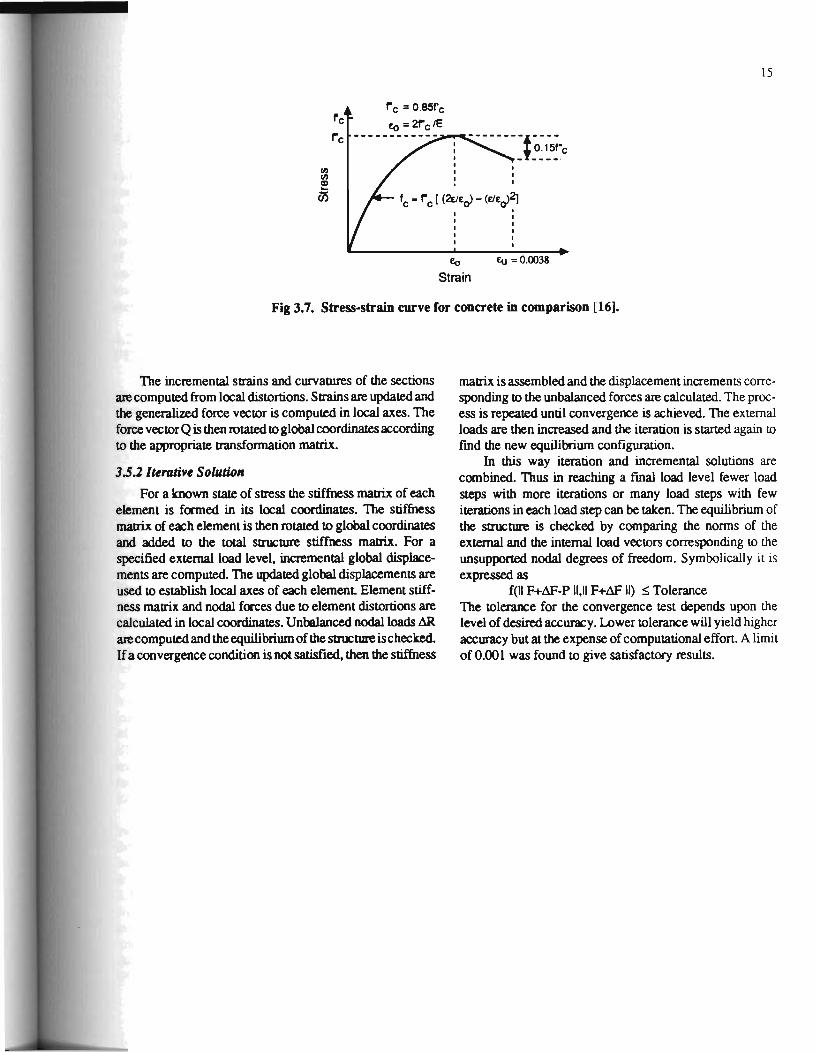
3.4 MATERIAL NONLINEARITY It was mentioned earlier that in the fiber model mem­

bers are divided into longitudinal fibers and each fiber is subjected to constant normal stress and strain over its area. Thus inclusion of material nonlinearity in the fiber model becomes simple in that only uniaxial stress strain relation­shipofthe materials is required. For a given strain in a fiber, the tangent modulus of the fiber is computed as the slope of the stress-strain curve for that particular type of fiber.

The stress strain relationship for the reinforcing steel is assumed to be elasto-plastic as shown in Figure 3.6. For a known strain, the stress is found by simply multiplying the strain by the elastic modulus of the steel. If the stress is grea1er than the yield stress, the stress is taken as the yield stress and the elastic modulus as zero. Arbitrarily, the steel is considered to fracture if a fiber strain reaches one percent [25]. There have been many theoretical curves proposed by different authors describing the constitutive relationship of concrete in compression. In this study the stress-strain relationship suggested by Hognestad [16] is adopted and is shown in Figure 3.6. The Hognestad curve has been shown to give good results for concrete not confmed by la1eral ties [23,25]. The concrete is assumed to have no tensile strength.

14

y

Strain

Fig 3.6. Stress-strain relationship for reinforcing steel.

3.5 SOLUTION PROCEDURE A combination of incremental and iterative solutions

with moving coordinates is used to trace the behavior of the structure. The advantage of using moving coordinates is that large deformations can be accommodated. In the general structural equation, given by Equation (3.15), ~ is the difference between the specified external loadings and the internal nodal forces due to the element distortions. Thus~ represents the tmbalanced nodal loads which must be zero for equilibrium of the structure. The iterative solution seeks a configuration such that the residual force is zero. The loads are applied in several increments to fmd the strucwral behavior at various stages of loading.

3.5.1 Computation of Element Distortions

Under a specified level of external loads, the structure deforms inducing internal nodal loads. Consider a vertical element in global coordinates as shown in Figure 3.4a. Figure 3.4b represents the equilibrium position of the ele­ment under a specified load level From the global displace­ments of nodes A and B the length androWion of the element can be computed as

X= U. • UA

y = v.- VA+ L, z = w1 ,.·--;;w...._,----;;---;;-. Lo = .J(x1+ yz+ zll

tan8x = z/ y tan8z = x/ y

where u, v, ware the global displacements of nodes A and B and L is the original length of the elemenL If the load level

I is now in~ the structure deforms and appears as in Figure 3.8c. The resulting incremental displacements are a combination of rigid body motion and distortion of the element. As internal forces are developed due to distortions only, the rigid body motion is subtracted and a local axis for the element is established. For the deformed configuration the following relationships hold true.

=\. = .1~ - .1u1 + x YL = .1vz- .1v• + Y ~ = .1w,- .1w, + z L ="(=\_l+yLl+Zi..l)

tan9Xo = 21.. I y L tan9Zo = =\. I y L

where .1u, .1v and .1w are incremental nodal displacements in global coordinates. The distortion corresponding to local coordinates of the element is given by

.1vBL = L- L0

~&AI.=~ ... + (ex- 9xo) ~dL =~ .. + (ex- exo) ~aAL = .141,..- ( 9z - 9Zo) ~dL =.141 .. - ( ez- 9zo) .1u = .,:\n_ = .1v = .1w = .1w =.., =.., AL IlL AL AL BL 'l'yAL 'l'yBL

=0 In these expressions suffixes A and B are for element nodes, and suffix L indicates the deformations correspond to local coordinates. The distortions for a horizontal member can similarly be derived. Figure 3.5 shows the original and equilibrium positions of a horizontal member. Figure 3.8b represents the deformed configuration under incremental load. The nonzero element distortions for this element are

.1v._ = L- L0

~&AI.= -~yA + ( 9y- 9yo) ~a-.= -~yl + ( 9y- 9yo) ~aAL = .141,.. + ( 9z- 8Zo) ~JilL= .141,.. + ( 9z - ezo)

In this case X= IL- u + L

II A I

y =v1 -vA z =w1 -wA tanSy = z/ x tan9z = y I x tanSy 0 = 21.. I =\. tan9Zo = yL/ =\_

Cl) Cl)

15

~ Ci5 'c- r c [ (2Eieo>- (fieo>2J

I

Eo Eu = 0.0038

Strain

Fig 3.7. Stress-strain curve ror concrete in comparison [16].

The incremental strains and curvatures of the sections are computed from local distortions. Strains are updated and the generalized force vector is computed in local axes. The force vector Q is then rotated to global coordinates according to the appropriate ttansfonnation matrix.

3.5.2 lttrativt Solution

For a known state of stress the stiffness matrix of each element is formed in its local coordinates. The stiffness matrix of each element is then rotated to global coordinates and added to the total structure stiffness matrix. For a specified external load level, incremental global displace­ments are computed. The updated global displacements are used to establish local axes of each element Element stiff­ness matrix and nodal forces due to element distortions are calculated in local coordinates. Unbalanced nodal loads ~ are computed and the equilibrium of the structure is checked. If a convergence condition is not satisfied, then the stiffness

matrix is assembled and the displacement increments corre­sponding to the unbalanced forces are calculated. The proc­ess is repeated until convergence is achieved. The external loads are then increased and the iteration is staned again to fmd the new equilibrium configuration.

In this way iteration and incremental solutions are combined. Thus in reaching a fmal load level fewer load steps with more iterations or many load steps with few iterations in each load step can be taken. The equilibrium of the structure is checked by comparing the norms of the external and the internal load vectors corresponding to the unsupponed nodal degrees of freedom. Symbolically it is expressed as

f(ll F+&"-P 11,11 F+&" II) ~Tolerance The tolernnce for the convergence test depends upon the level of desired accuracy. Lower tolerance will yield higher accuracy but at the expense of computational effort. A limit of 0.001 was found to give satisfactory results.

16

(a) For vertical members . (b) For horizontal members

Fig3.8. Displaced configuration or members.

CHAPTER 4. VALIDATION OF COMPUTER PROGRAM

4.1 INTRODUCTION 1lle results of the present nonlinear analysis were

checked for a variety of structural configurations and load combinations. Configurations ranged from a single member to frames. The loading was varied from axial load with in­plane loads or moments to biaxial loads. The accuracy of the computer results was established fliSt by checking the effect of the number of segments per member and the size of the load steps. The experimental and analytical results of several investigations were used to verify the predictions of the present formulation.

4.2 EFFECT OF NUMBER OF SEGMENTS PER MEMBER

The monotonic convergence of the computer results was verified by checking the results obtained by refming the mesh. This also established the number of segments or elements required to model the behavior of one member. The results of the typical cases are presented in Figs 4.1 through 4.3.

Figure 4.1 shows the load deflection curves for a canti­lever subjected to simultaneous action of axial load and horizontal loads. The length of the member was divided into 2,4, 8 and 16 segments giving the segment length to section depth ratios of 5, 2.5, 1.25 and 0.625 respectively. No graph is shown for the sixteen segments, as the load deflection values for the eight and sixteen segments were the same. The predicted ultimate compressive axial loads for four, eight and sixteen segments are 305, 300 and 296 kips respectively.

The results for a pin ended column are shown in Fig

loads (H) for 16,32 and64 segments were 13.31, 12.81 and 12.78 kips respectively.

From the above results, it may be concluded that seg­ments with length to depth ratios of 1.0 to 1.5 would be satisfactory for columns. It is envisaged that a lower ratio would be necessary for beams due to the higher moment gradient.

4.3 EFFECT OF THE SIZE OF LOAD STEPS

To check: the effect of the size of the load steps, a specified load level was applied in one step. The solution was then compared with the same load level but applied in several increments. No graphs are shown for these cases as there was no difference between the load deflection values. A combination of incremental and iterative solutions is used in this study. For each load increment, the structural equa­tions are solved using an iterative technique until equilib­rium of the structure is established. Therefore the solution is not affected whether a specified load is applied in one step or in several increments. However, to trace the behavior of the structure, loads should be applied in several increments. There are computational advantages in applying relatively larger loads when the effect of nonlinearities are not severe. The size of the load steps should be reduced near the failure of the structure.

30 4- 2Segments

- 4 Segments £ 8 Segments

~p ~Hz

4.2. The geometric layout and material properties of the column are essentially the same as the previous case, except for the different suppon conditions. The column "[ is again divided into 2, 4, 8 and 16 segments. An axial ;g.

20 load of 1000 kips was applied fliSt and kept constant ~ while the horizontal loads were increased proportion- -g ally until failure. A similar behavior was found for eight .3 and sixteen segments. The ultimate horizontal loads for

~Hx

four, eight and sixteen segments are 134.2, 132.6 and 129.4 kips respectively.

The frame of Fig 4.3 was analyzed to establish the number of segments required for a member accounting the interaction of beams and columns. The vertical members of the frame were divided into 2, 4, 8 and 16 segments giving segment length to depth ratios of 5.4, 2.7, 1.35 and 0.675 respectively. The size of segments were kept constant in both horizontal and venical members. A tocal of eight segments implies four ele­ments for the beam and two for each column.. The difference between the load deflection values for 32 and 64 segments were negligible. The ultimate horizontal

Iii c: 0

-~ ~ 10

4Hx- ~Hz- 0. 10"~

1(: - 4.941 ksl Fy • 60 ksl

24 in.

: 111 : 24 in .

Cover- 2.4 in .

o'-------_.--------~------~------~4 0 1 2 3

Lateral Tip Deflection, dX (in.)

Fig4.1. FJrect of number of segments.

17

18

Iii' a. % )(

:I: -o" co 0

...J

iii c: 0 -~ .... 0 :I:

160 ... 2 Segments

- 4 Segments • 8Segments

120

P- 1000 kips

80 ,~mi Hx

Hx- Hz 241n.

40 rc- 4.941 ksl : 111 : 241n.

Fy- 60 ksl Cover- 2.41n.

0 __________ _. __________ ~--------~-----

0.0 0~ OA 0~

La1eral Deflection a1 Midspan, 4X (in.)

15 ... 8 Segments

- 16 Segment& a. 32 Segments

Iii' 10 a. p

;g_ ~ ..9 iii c: 0

-~ 0 :I: 5

H 2161n. 1081n.

10 ln.

EJ 10 in . . Column

Cover- 2.5 ln.

rc-3ksl Fy • 60 ksl

10 ln.

D121n. D Beam

0._------~~------~--------_.--------~ 0.0 0.5 1 .0 1.5 2.0

Lateral Deflection (in.)

Fig 4.2. Effect or number or segments.

Fig 4.3. Enect or number or segments.

4.4 COMPARISON WITH ANALYTICAL RESULTS

Chen and Atsuta (7] have presented several ultimate strength interaction curves for simply supported square columns under biaxial bending. Their study uses Newmark's method [ 19] for the numerical integration of the moment-curvature relationships. The results are given for combinations of axial compressive loads (P), reinforcement ratios (As/ab), slenderness ratios (L/a), steel ultimate strength _(FY) and the con~te compressive strength (f' )· The secuon and the material properties of the column are shown in Fig 4.4. Two ratios of length to section depth (l.Ja) were selected for comparative study. The results of Chen and Atsuta are compared with the present model and are shown on the same figure. The columns were divided into eight segments while Chen and Atsuta used nine seg­ments. The results are in very good agreement.

Diaz [ 10] analyzed the frame shown in Fig 4.5 using the complex fiber model. The fiber model of Diaz uses the large deformation theory of beam-columns under uniaxial bend­in~. The results of the complex fiber model are compared w1th the present formulation and are shown in Fig 4.5. Excellent agreement is found between the two results for the moment M A. The moment ~ predicted by the present formulation is slightly higher than the one obtained with the complex fiber model.

4.5 COMPARISON WITH EXPERIMENTAL RESULTS

In the absence of experimental results for planar frames under spatial loads, the nonlinear analysis program was used to analyze several rectangular frames under in-plane loads and single columns under biaxial loads. The results for the typical struc­tures are discussed below.

19

points. -~e load deflection curve predicted by the present model IS tn excellent agreement with the test results. The ultimate load predicted is 13.94 kips while the measured value was 14.88 kips.

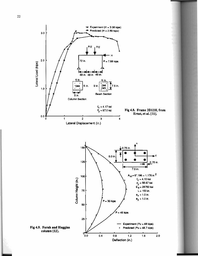
Frame 2Dl2H: This frame had the same general properties as frame 2012 except for the lower concrete strength. In addition to vertical loads, there was a horizontal load applied as shown in Fig 4.8. During the test the vertical load wasappliedfU"Standkeptconstantat 7.88 kips while the horizontal load was increased The same loading sequence :"'~used to predict the behavior of the frame. Except for the nutial stages where tension in the concrete plays a major role, the agreement between the predicted and the measured values is good. Since the program shows a good agreement for ~ost frames at early stages, it is envisioned that the omission of the tensile strength of concrete is not the LOtal cause for the difference found in this case. The predicted horizontal load was 2.89 kips. The ultimate load from the experiment was 3.08 kips which differs from the predicted value by 6%.

Farah and Huggins [ 12] tested a column pinned at the ends with the axial load applied eccentrically. The cross section and material properties of the column are shown in Fig 4.?. In the same figure the deflections measured along the diagonals are shown together with the analytical predictions. The results of the present formulation are in excellent agreement with the test results. The ultimate load predicted is 48.7 kips while the measured value was 48 kips.

0.20

0.15

tc -4.941 ksi Fy- 60 ksi

_f_ rcab -0.50

As ab- 0.0325

Fergusonetal. [13] testedaseriesofsinglepanel frames. From this series, frame L3 was chosen for the verification of the computer results. Geometric char­acteristics and material properties of the frame are shown in Fig 4.6. The proportional loading was used as in the test program. The vertical load versus lateral deflection is also shown on the same figure. The basic shape of the load..<Jeflection curves are almost iden­tical. The ultimate load predicted by the nonlinear analysis was only slightly highC"J" than the measured value.

~ 1~ 0.10

• Chen and Atsuta - Present Method

Ernst er aJ. [11] tested fifteen frames under various combinations of vC'J'tical and lateral loads. Two frames were selected to check the accuracy of the program.

Frame 2Dl2: The geometry and material properties of this frame are shown in Fig 4.7. The frame was loaded with concentrated loads at third

0.05

0.00 L.-___ .._ ___ ...._ ___ .......,J ___ __.

0.00 0.05 0.10 0.15 0.20

Fig 4.4. Strength interaction curves for square sections.

20

4.6 SUMMARY The results presented in this chapter indicate that the

present model can be used to predict accurately the behavior of planar concrete frames under spatial loads. In all cases investigated, the analytical predictions were close to the experimentally observed behavior and other analytical re­sults. Although there were some discrepancies between the predicted and the experimental load deformation curves, the ultimate capacity was generally in very good agreement

500

400

10in. 10in.

The accuracy and monotonic convergence of the com­puter results were verified by analyzing several structures. It was found that segments of length to depth ratios of 1.0 to 1.5 would be satisfactory for both vertical and horizontal members. The results for a specified load are independent of the number of load increments in which the desired load level is divided.

1:·"":1··~ I ~ .. }2 ~ Column Beam

100

Cover • 2.5 in.

f(:- 3 ksl Fy• 60 ksl

- Dlaz's Results • Present

0~----------~----------~----------~----------~~-----~ 0 2 4 6 8 10

Horizontal Load, H (kips)

Fig 4.5. Frame Cll (cue l) from Diaz [10].

en .Q. ~ "0

<'CI 0

...J

Iii .2

35

30

25

en 20 a. ~ a.. -o

<'CI 0

...J 15

10

5

... Experiment (P- 31 .0 kips) • Predicted (P • 32.4 kips)

6 1n. ~ t...:......:::: 3-3116 in.

Beam Section

6 in.

~4in. l.:..-=-.:J

Column Section

Fig 4.6. Frame L from Ferguson, et al. h3J.

Fy - 57.45 ksi

~'c• 3.2 ksi

15

10

5

-...

0._--------~----------~--------~ 0 1 2 3

61n. G61n. !+-.~

51n. Column Section

Lateral Deflection (in.)

P/2

72 in.

6 in.

91n.[ ):f []7.51n.

Beam Section

1(:- 5.92 kal Fy -67.0 ksi

Fig 4.7. Frame 2Dl2, from Ernst, et al. (11].

0~--------~----------~--------~ 0 1 2 3

~rtical Deflection at Midspan (in.)

21

22

(i) a. ~ "0

CIS 0

....J

~ CD iii ....J

3.0

2.0

1.0

- Experiment (H - 3.08 kips) .- Predlcled (H - 2.89 kips)

~---~-......

72 in . p- 7.88 kips

I• Ill• Ill• ~ 48 in. 481n. 48 in .

6 in.

GJ 6 in . . 1+-+1

5 in. Column Section

Sin.

9 1n. l ~~=~IJ7.5in. Beam SectJon

1(:- 4.17 kSI

Fy - 67.0 l<si 0 .0 ...._ ___ ....... ____ ....~.... ___ ___..__ ___ _.

0 1 2 3 4

Lateral Displacement (in.)

Fig 4.8. Frame 2D12H, from Ernst, et al. [11].

0.75 in. . ~· • 5.0 in ..._ __ t-.... z

• • • ... ,----~~ ... ~75in. 14·---~~

7.0in.

125

100 Ast• 6".196- 1.1761n.2 - 1(:- 4.10 ksi ~ Fy • 55.67 ksi .E .2» E s- 28750 ksi CD :r: 75 L· 153 in. c ex- 1.0 ln. E :;:, ez- 1.0 ln. 0 ()

50

25

Experiment (Pu • 48 klps) Fig 4.9. Farah and Huggins

column [12]. • Predlct8d (Pu • 48.7 klps)

0 .0 0.4 0.8 1.2

Deflection (in.)

1.6 2.0

CHAPTER 5. RESULTS AND DISCUSSION

5.1 INTRODUCTION In Chapter 2, various procedures for analyzing bridge

bent columns were described. The details of the second order nonlinear analysis formulation were presented in Chapter 3. The objective of this chapter is to compare the results from the linear and nonlinear analyses with those obtained from the TSDHPT approximate procedure. The current procedure of determining the design column forces and moments is compared with the linear frame analysis. The nonlinear analysis is used to investigate the suitability of the effective length factor used in the approximate procedure. The effect of the foundation flexibility on the overall behavior is finally investigated.

5.2 BENT CONFIGURATION Five typical bents were selected for the comparative

study. These bents are either in service or will be built in the near future. The geomenic characteristics and material properties of these bents are shown in Figs 5.1 through 5.10. Bents 1 and 2 are identical except for the number of girders and their spacing. Also, the arrangement of girders is not exactly symmetrical in bent 2. Bents 3 and 4 consist of five and four columns respectively, with eleven girders arranged symmenically. Bent 5 consists of three columns with an unsymmetrical arrangement of girders. The skew angle of these bents represents the angle between the normal to the longitudinal center line of the bridge and the plane of the bent.

5.3 LOADS ON BENTS As mentioned earlier, the TSDHPT has identified

AASIITO load groups I, II and III as the critical load combinations for the design of typical Texas highway bridge bents. These load groups are used in computing the column axial forces and bending moments in all analysis procedures. The computation of these loads is carried out in accordance with the AASIITO specifications. The capacity reduction factor of 0.70 is used in computing the nominal design loads [29]. The gravity and lateral loads for various bents are summarized in Table 5.1. The design wind velocity was assumed 80 miles per hour in computing the wind loads. The wind loads (Table 5.1) correspond to the wind direction perpendicular to the longitudinal axis of the bridge. The AAS liTO HS20-44 standard truck and lane loads are used in computing the live loads on the bridge. In computing the gravity loads of Table 5.1, the live loads on the bridge were disnibuted equally between the beams. A dead load combi­nation factor Bx, of 1.0 is used in this study. Hx and Hz are in­plane and out of plane horizontal loads respectively. These forces are equivalent loads at the bent cap level. L represents the column unsupported length (including depth to fixity)

23

and the minimum radius of gyration of the column section is designated by r.

In the linear frame analysis, wind loads corresponding to five AASIITO specified wind directions were used. The live loads were computed using the two approaches de­scribed in Chapter 2. The first method distributes the live loads evenly between the beams. The second approach considers the variable live load positions on the bridge deck.

5.4 APPROXIMATE PROCEDURE VS LINEAR FRAME ANALYSIS

The results of the linear frame analysis are compared with the column design moments and forces of the current TSDHPT approximate procedure. The moment magnifica­tion method of the ACI code is used to approximate second order effects. The method requires the selection of an effec­tive length factor(k) for both axes of bending. Since the bent is treated as a cantilever for the out of plane loads, it would be appropriate to use a k-factor of 2.0 for out of plane bending. For inplane bending, the k-factor should be com­puted using either the alignment charts or empirical equa­tions [15] recommended by the code. The moments com­puted for both the in plane and out of plane loads are ampli­fied independently according to their associated magnifica­tion factors. This procedure of moment magnification, rec­ommended by the code, will be considered later in this chapter. The approximate procedure assumes an effective length factor of 1.25 for both inplane and out of plane bendings. The same k values are also used in computing the amplified design moments in the linear frame analysis. The resultant of the in plane and out of plane moments is found using the Pythagorean theorem. The results obtained in this study are presented in the next subsections.

5.4.1 Group I Loads

The column axial forces predicted by the approximate and linear frame analysis procedures are shown in Figs 5.11 and 5.12. Each data point on the graph represents a column. The linear analysis yields axial load and associated moment for each column. For example, bent 1 with three columns will yield three data points since only one value of Bx, is used in this study. The data points are reduced considering the symmetry of results. The column axial loads from the linear analysis in Fig 5.11 were obtained by distributing the total live loads equally between the beams. Figure 5.12 indicates the effect of variable truck position across the deck. No graph is shown for bending moments in this load group, as minimum eccentricity criterion of AASIITO was found to govern in all cases.

The column axial forces from the two analysis proce­dures are in good agreement for bents 1 through4 (Fig 5.11),

24

the maximum difference being less than 10%. For bentS, the column axial load predicted by the linear frame analysis is about 35% higher than the results of the approximate analy­sis. The approximate procedure generally underestimates the design axial forces (Fig 5.12) when the effect of variable IIUck positioning is considered. For bent 5, the difference is about 50%.

5.4.2 Group II Loads

Figures 5.13 and 5.14 represent the ratios of the column axial forces and moments predicted by the two analysis procedures. For each column, five data points are obtained, one for each wind direction. (AASHTO specifies five wind directions to be considered in computing the design wind loads). It may be noted that the live load is absent in this load group. It is observed (Figs 5.13 and 5.14) that the approxi­mate procedure underestimates axial forces in some col­umns and overestimates the associated inplane bending moments for bents 1 through 4. For one column of bent 5, the approximate procedure underestimates both the column moment (20%) and axial forces (32%). However, for an­other column of this bent the axial load predicted by the approximate procedure is almost twice that from the linear analysis. The moments predicted by both procedures are within 5%.

5.43 Group III Loads

The results obtained for this load combination are shown in Figs 5.15 through 5.18. The column axial forces and bending moments from the linear analysis procedure (Figs 5.15 and 5.16) are based on the live loads distributed equally between the girders. In this load group, the approxi­mate procedure generally overestimates the design mo­ments {bents 1 through 4 ). The ratio of axial loads predicted by the two procedures are within 10%. The ratios of the column moments and axial loads for bent 5 are similar to those for load group II. Figures 5.17 and 5.18 represent the effect of variable live load position. The maximum column moments and corresponding axial loads are included in these figures. It may be seen that the column moments and axial forces, computed using the two analysis procedures, are generally in good agreement (within 10%) for bents 1

through 4. The results from the approximate procedure are unconservative for bent 5, in terms of either higher moment and low axial load or high axial load and associated moments when compared with the linear frame analysis values.

5.4.4 Discussion of Resulls

For load group I, the axial forces predicted by the TSDHPT approximate procedure agree well with the linear frame analysis values {bent 1 through 4 ), when live loads on the bridge are distributed equally between the girders. For bent 5, the approximate procedure underestimates the axial force in one column which is balanced by overestimating the force in another column. The current office procedure, however, generally underestimates the axial forces when the variation in live load positions over the deck is considered. The implication of these results depends on the AASHTO load combination controlling the design. If the design is controlled by this load group, the larger column axial forces and minimum moment would be the critical sib.lation as the design is governed by the axial strength of the column.

For load combinations II and III, the design or strength of columns is typically governed by the bending action as the axial loads in columns are generally less than the corre­sponding axial loads at the balanced condition. (The bal­anced condition is defined as a combination of axial load and moment whe-n the yielding of steel and the crushing of concrete occur simultaneously). Therefore, the higher moments and lower axial loads predicted by the approximate procedure are conservative for bents 1 through 4. For bent 5, the approximate procedure overestimates the axial force in a column resulting in an unconservativedesign situation. As the bent geometry deviates from the typical geometries, the uncertainty relating to the approximate procedure increases. The amounts by which the inplane bending moment is overestimated and the axial force is underestimated by the approximate method are unpredictable. For the range of variables investigated. it was observed that for the load group m, varying the live load positions on the bridge deck does not drastically change the results compared with the values for live loads distributed equally between the beams. This may be attributed to the low percentage of gravity loads contributed by live loads in this load group.

1.75'

0 4.75' 17.75'

Forward Span Length • 105.30 It Ba~ward Span Length • 105.30 It Skew Angle - 0.00 Degrees Degree of Curve • 0.00 Degrees Rail Height • 2.0 It Weight of Rail - 0.300 kips/It Weight of Beam • 0.516 kips/It Cap Length - 35.5 It Column Height • 22.0 It Strength of Concrete • 3600 psi

30.75' 35.50'

Number of Lanes Number of Beams Number of Columns Depth of Beam Slab Depth Slab Width Beam Spacing Column Spacing Depth to Fixity Steel Yield Stress

-3 -6 -3 • 4.5 It • 7.75 in. - 38.25 It - 6.4 ft -13.0ft • 5.0 It -60 ksi

Fig S.l. Layout and material properties or Bent 1.

391n.

D D ...

. . 36 in . • •

. . . . D-110

-15

-15

-110

Cover - 3.26 in.

Section-A Sectlon-8 Section-C

Bent Cap Sections

Sections along Cap Leng1h (Ftg 5.1)

Cover - 3.46 ln.

Dlame!Br- 36 in.

Columns

From

0.00

4.75

12.00

17.75

23.50

30.75

To Section

4.75 c 12.00 A

17.75 B 23.50 B 30.75 A

35.50 c

Fig 5.2. Cross sections or bent cap and columns or Bent 1.

25

26

0 4.75' 17.75'

Forward Span Length • 105.30 It Backward Span Length - 105.30 It

30. 75' 35.50'

-3 -6

Skew Angle - 0.00 Degrees

Number of Lanes Number of Beams Number of Columns Depth of Beam Slab Depth

-3 Degree of Curve - 0.00 Degrees Rail Height • 2.0 It Weight of Rail - 0.300 kipstlt Weight of Beam - 0.516 kipstlt Cap Length - 35.5 It Column Height • 22.0 It Strength of Concrete - 3600 psi

Slab Width Beam Spacing Column Spacing Depth to Fixity Steel Yield Stress

-4.5 ft - 7.75 in . - 38.25 It - 8.0 It - 13.0 It - 5.0 ft -60 ksl

Fig 5.3. Layout and material or Bent 2.

391n. -110

-15 36in.

-15

0 -110

Cover - 3.26 in.

Section-A Section-S Section-C

Bent Cap Sections

Sections along Cap Length (Fig 5 3)

Cover • 3.46 ln.

Diameter • 36 ln.

Columns

From

0.00 4 .75

14.25 17.75 21.25 30.75

10 Section

4.75 c 14.25 A 17.75 B 21 .25 B 30.75 A 35.50 c

Fig 5.4. Cross sections or bent cap and columns or Bent 2.

2.028'

0 6 .83' 29.83' 52.83' 75.83' 98.83' 1 05.66'

Forward Span Length - 80.0 It Number of Lanes -6 Backward Span Length - 75.0 It Number of Beams -11 Skew Angle • 30.0 Degrees Number of Columns -5 Degree of Curve -0.00 Degrees Depth of Beam - 3.33 It Rail Height - 2.0 It Slab Depth • 8.0 in. Weight of Rail - 0.330 kipslft Slab Width - 94.0 It Weight of Beam - 0.516 kipslft Beam Spacing -10.161 It Cap Length - 105.60 It Column Spacing - 23.0 It Column Height - 24.0 It Depth to Fixity - 5.0 It Strength of Concrete • 3600 psi Steel Yield Stress -60 ksi

Fig 5.5. Layout and material properties or Bent 3.

33 in .

33;,DI~::::J ...... . D-111 -110 -15 -15

-111

Cover • 3.33 ln.

Section-A

Cover • 2.94 in.

Diameter • 30 in.

Columns

Section-B Section-C Section-D

Bent Cap Sections

Secti ·ons al()nQ Cap Length (Ftg 5. 5)

From To Section

0.00 6.83 D

6.83 14.08 A

14.08 38.83 B

38.83 67.33 c 67.33 91 .58 B

91.58 98.83 A

98.83 105.66 D

Fig 5.6. Cross sections or bent cap aod columns of Beot 3.

27

28

Section-A

-14--1.75'

0 7 .75' 30.42'

Forward Span Length • 109.5 ft Bad(ward Span Length • 109.5 ft Skew Angle • 0.00 Degrees Degree of Curve • 0.00 Degrees Rail Height • 2.0 ft Weight of Rail • 0.330 kipsltt Weight of Beam • 0 .516 kipsltt Cap Length • 83.50 ft Column Height • 45.0 ft Strength of Concrete • 3600 psi

53.08' 75.75' 83.50'

·6 • 11

Number of Lanes Number of Beams Number of Columns • 4 Depth of Beam Slab Depth Slab Width Beam Spacing Column Spacing Depth to Fixity Steel Yield Stress

• 4.5 ft • 8 .0 in. • 87.0 ft • 8.0 ft • 23.0 ft • 6 .0 ft • 60 ksi

Fig 5. 7. Layout and material properties or Bent 4.

-111

. -16

• -16

-111

Section-B Section-C

••••••••• -111 Sections along Cap Length (Fig 5. 7)

42 in . • -16

• -16

• -111 '-----....1

Section-D Secllon-E

Bent Cap Sections

Cover • 3 .25 in.

Diameter • 36 in.

Columns

Fig 5.8. Cross sections or bent cap and columns or Bent 4.

From

0.00

7.75

16.25

22.42

30.42

38.42

45.08

53.08

61 .08

67.25

75.75

10 Section

7.75 E 16.25 A

22.42 B

30.42 A 38.42 c 45.08 D

53.08 c 61 .08 A

67.25 B

75.75 A

83.50 E

1.746' 1.623'

0 8 .0' 21 .25' 34.50' 40.50'

Forward Span Length - 80.03 It Number of Lanes -3 Backward Span Length - 80.03 It Number of Beams ·5 Skew Angle • 14.2 Degrees Number of Columns -3 Degree of Curve - 0.00 Degrees Depth of Beam - 4.17 It Rail Height - 2.0 It Slab Depth - 10.0 in . Weight of Rail - 0.330 kipslfl Slab Width - 42.0 It Weight of Beam - 0.516 kipslfl Beam Spacing - 9.28 It Cap Length - 40.50 It Column Spacing ~ 13.25 II Column Height - 23.0 It Depth to Fixity z 5.0 It Strength of Concrete • 3600 psi Steel Yield Stress -60 ksi

Fig 5.9. Layout and material properties of BentS.

33 in

33 in. •

Cover • 3.58 in.

Section-A

-111

• -18

. -18

. -111

Seclion-B

Bent Cap Sections

Cover • 3.58 in.

Diameter • 30 in.

Columns

Sections along Cap Length (FIQ 5.9)

From To Section

0.00 15.50 B 15.50 27.00 A

27.00 40.50 B

Fig 5.10. Cross sections or bent cap and columns or Bent 5.

29

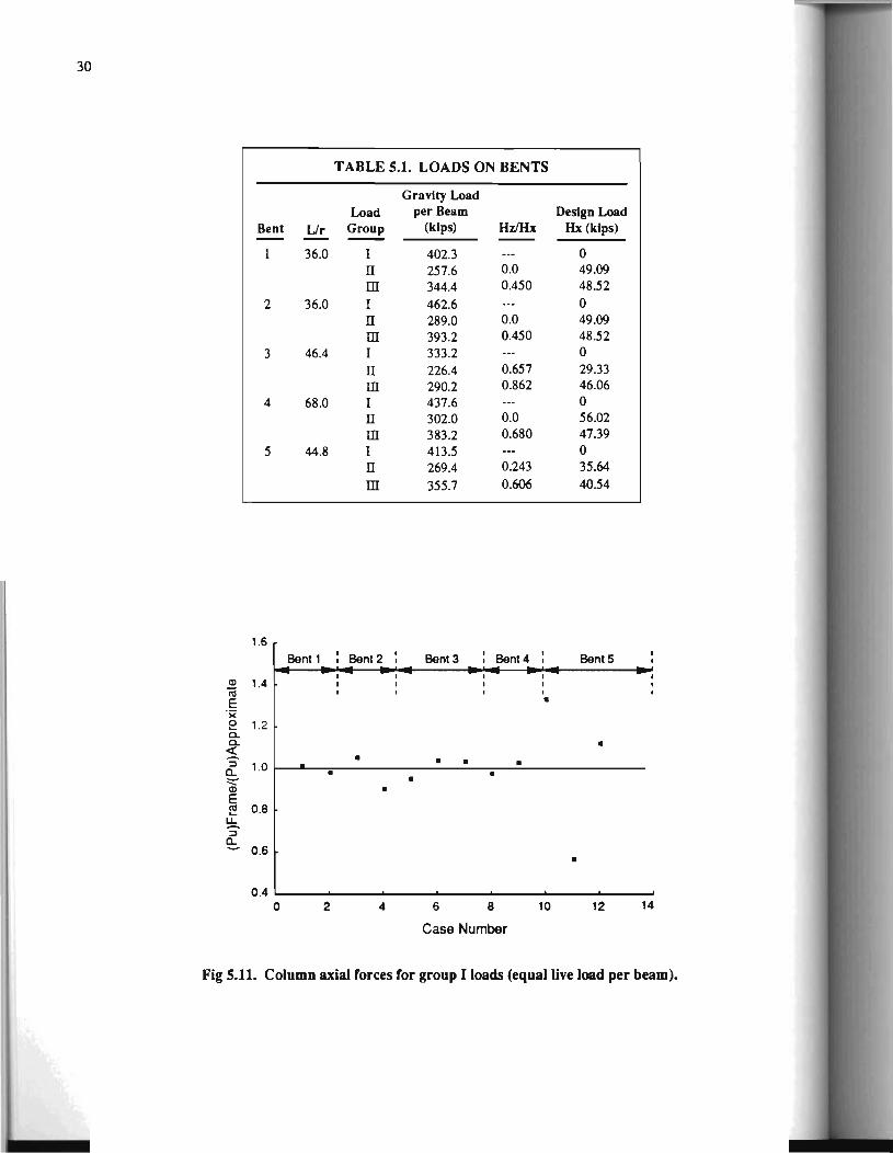
30

TABLE 5.1. LOADS ON BENTS

Gravity Load Load per Beam Design Load

Bent Ur Group (kips) HliHx Hx (kips)

36.0 I 402.3 0 II 257.6 0.0 49.09 III 344.4 0.450 48.52

2 36.0 I 462.6 0 II 289.0 0.0 49.09 III 393.2 0.450 48.52

3 46.4 I 333.2 0

II 226.4 0.657 29.33 III 290.2 0.862 46.06

4 68.0 I 437.6 0 II 302.0 0.0 56.02 III 383.2 0.680 47.39

5 44.8 I 413.5 0 II 269.4 0.243 35.64

m 355.7 0.606 40.54

1.6 Bent1 Bent2 Bent3 Bent4 Bent5

(I) 1.4 co I

E • ")(

e 1.2 a. a. • <t • • • • ::::1 1.0 a.. • • :::::- • (I)

E !U 0.8 .... ~

::::1 a.. ~ 0.6

•

0.4 0 2 4 6 8 10 12 14

Case Number

Fig 5.11. Column axial forces for group I loads (equal live load per beam).

31

1.6

1.4 • Cll iii • • E • ·x 0 1.2 • .... a. • • • a. • ~ • :::1 1.0 a.. :::::-Cll E

0.8 Ill .... I%. • :::1 e:. 0.6 Bent 1 I Bent2 Bent3 I Bent4 BentS

0.4 0 2 4 6 8 10 12 14

Case Number

Fig 5.12. Column axial rorces ror group I loads (variable live load position).

1.6 Bent 1 1 Bent 2 Bent3 Bent4 Bent 5

-20 40 60 80

Case Number

Fig 5.13. Design axial rorces for group ll loads.

32

1.4 Bent 1 Bent2 I Bent3 Bent4 BentS

<l)

iii E 1.2 ')( rP 0

"" ,_ a. a a. <:

rP a ::I 1.0 ~ a a a/' a a a a a a a a ...... a d' d'a a a rl'a a <l) a E rl' a a rP a a a

"' a a a ,_

a a a u.. 0.8 a

S' ~ rl' a

a

0.6 0 20 40 60 80

Case Number

Fig 5.14. Design forces for load combination II.

1.6 Bent 1 Bent2 Bent3 Bent4 Bents

<l) 1.4 iii -E ')( 0 ,_ 1.2 a. a. -<: aaaaa - - - ~ ::I 1.0 ~ - -...... - -<l)

E "' ,_ 0.8

Y::. ::I

~ 0.6 -0.4

0 20 40 60 80

Case Number

Fig S.lS. Design axial forces for load group ill (equal live load per beam).

33

1.3 Bent 1 Bent2 Bent3 Bent4 BentS

Q) 1.2 (ij E )(

0 1.1 '-a. 'b a. """' <(

::J 1.0 ::E • . a a a ./'~ a ~ a a a a a a; a a a a a a

a a a a a E a a

ro 0.9 a a a '-u.. a a a ::J

~ a a 0.8

0.7 0 20 40 60 80

Case Number

Fig 5.16. Design moments for load group ill (equal live load per beam).

1.6 Bent1 Bent2 Bent3 Bent4 BentS I I

Q) 1.4 (ij -E ·x 0 1.2 '-a. a. -~ ...... - - -::J 1.0 e:.. - -a; ...... ...... E -ro 0.8 '-

~ ::J a.. ~ 0.6 -

0.4 0 20 40 60 80

Case Number

Fig 5.17. Design axial forces for load group ill (variable live load position).

34

1.3 Bent 1 Bent2 Bent3 Bent4 BentS

CD 1.2 iii E a a ·;;:

"a 0 1.1 a a. ""- ...._aa.-a. ~ aaaaa ::J 1.0 a

:E a ...... a a CD a

a E 0.9 a co

u: a a

::J

:E 0.8

0.7 0 20 40 60 80

Case Number

F. 5 18 Des•"gn moments for load group ill (variable live load position). •g ..

5.5 APPROXIMATE PROCEDURE VS NONLINEAR ANALYSIS

In this section, the results predicted by the nonlinear analysis are compared with those obtained from the TSDHPT approximate procedure and the ACI moment magnifier method. The moment magnification method of ACI assumes an effective length factorof2.0 for out of plane bending. The k factor for inplane bending was computed using the alignment chart of the Code [2]. In the no~li~ear analysis, the gravity loads on the bridge were div1ded equally between the girders. The gravity loads on beams were applied first and kept constant. The biaxial lateral loads were then increased proportionally until failure. Three modes of failure are recognized: (a) compression failure when the specified compressive strain of concrete is reached; (b) tension failure when the specified steel ultimate strain is reached; and (c) stability failure when the tangent stiffness mauix of the system becomes singular or negative. The loads applied on bents are given in Table 5.1.

5.5.1 Load-Deformation Curves

The load-deflection curves for all five bents and for load combinations 11 and III are presented in Figs 5.19 through 5.28. The in plane and out of plane lateral deformations are plotted against the in plane horizontal loads (Hx). It .may be observed that for a given load, theoutofplanedeflecuonsare generally higher than the inplane deflections_. Th~s is d~~ to the cantilever action in the out of plane direcuon, m addiuon to the relative magnitude of the lateral loads. The maximum lateral loads and the failure modes for various bents, pre­dicted by the nonlinear analysis are summarized in Table

5.2. The analysis of each case is as expected. The change in the initial slope of the load deflection curve is an indication of the initiation of flexural cracks in concrete. The yie'lding of rebars may be responsible for a subsequent change in the slope. It may be seen that bents 3 and 4 (Figs 5.23, 5.24 and 5.26) experienced a large deflection prior to failure. The program showed a material failure in the structure. It is envisioned that such a large deformation may be an indica­tion of the stability failure.

5.5.2 Predicted Axial Loads vs Design Axial Forces

The variation of the column axial forces with the gravity loads on beams for various bents is presented in Figs 5.29 through 5.33. The column axial forces computed using the TSDHPT approximate procedure are also included. From Figs 5.29 through 5.32, it may be seen that the axial forces predicted by the approximate procedure are in close agr~­ment with the analytical predictions. For bent5. the apprOXI­mate procedure underestimates the analytical predictions for one column. This is balanced by overestimating the axial force in another column. Recall that the bent 5 consists of five girders ananged unsymmetrically over the bent cap. These results are similar to those obtained from the linear frame analysis where live loads were distributed equally between the beams.

5.5J Predicted Moments vs Design Moments

The moments from the nonlinear analysis procedure are compared with the predictions of the ACI moment magnifier method and the TSDHPT approximate procedure. The results of this sbldy are presented, for each bent and for load groups 11 and 111, in the following subsections. In load

in on ng he nd he is

:a-

lty 29 he lffi

es :e-d-ns ia1 of .p. ar ly

re er lle ad ik1

35

300

250

2 3 4

In-Plane Lateral Deflection, ~x (in.)

Fig 5.19. Load-deformation curve for Bent 1 (load group II).

250 a In· Plane Deflection (.iX)

.. Out of Plane Deflection (..U)

200

Cil a. g 150 )(

I "0 D E F G H Ill

I I I 0 ...J

"ii! 100 Q) A B c iii

...J

Hz/Hx. 0.45 50

Gravity Load per Beam • 344.4 kips

o~------._------~------~----~~----~ 2 3 4 5

Lateral Deflection (in.)

Fig 5.20. Load-deformation curve for Bent 1 (load group ill).

36

350

300

250

(j) a. ;g, )( 200

::r: "0 ('CI 0 D E F G H ~

~ 150

I I I ! ~

A B c 100

Hz/Hx • 0

50 Gravity Load per Beam • 289.0 kips

0~ .................... ~ .................... ~ .................... -L .................... ~

0 2 3 4

Lateral Deflection (in.)

Fig 5.21. Load-deformation curve for Bent 2 (load group II).

250 a In-Plane Deflection (AX)

• Out of Plane Deftection (.U)

200

(j) 0..

~ 150 )(

::r: -o 0 E F G H ('CI

I I I 0 ~

n; 100 ..... Q)

CiS A B c ~

50 Hz I Hx • 0.45

Gravity Load per Beam - 393.2 klps

06-.......... -L ............... ._ .......... _. ............... ._ .......... -L .......... ~

0 2 3 4 5 6

Lateral Deflection (in.)

Fig 5.22. Load-deformation curve for Bent 2 {load group Ill).

37

100

80 a In-Plane Deflection (ru<)

.a. Out of Plane Deftection (6.Z)

Iii' CL.

~ 60 >< I

"0 F G H J K L ctl

I I I I I 0

....J

~ 40 Q)

ii:i ....J

A B c D E

20 Hz/Hx - 0.657

Gravity Load per Beam - 226.4 kips

0»-------~------~-------L------~------~ 0 2 4 6 8 10

Lateral Displacement (in.)

Fig 5.23. Load-deformation curve for Bent 3 (load group II).

80

60 a In-Plane Deflection (ru<)

.a. Out of Plane Deflection (6.Z)

Iii' CL. ;g_ >< I

"0 40 ctl 0

....J

iii ... .!! ~

F G H J K L

I I I I I A B C D E

20

Hz I Hx • 0.862

Gravity l.Dad per Beam - 290.2 kips

0~----------------~-----------------L--...----------L----------~ 0 2 4 6 8

Lateral Deflection (in.)

Fig 5.24. Load-deformation curves for Bent 3 (load group ill).

38

30 a In-Plane Deflection (rue)

.. Out of Plane Deflection (6l)

25

(/l 20 c.. ~ >< E F G H I J I -o

15 I I I I Cll 0

....J

iii .... <D A B c D cu

....J 10

HZ/Hx- 0.68

Gravity Load per Beam - 383.2 kips

5

0 __________ ._ ________ ._ ________ ~--------~

0 5 10 15 20

Lateral Deflection (in.)

Fig 5.25. Load-deformation curve for Bent 4 (load group II).

150

en 100 c.. ~ E F G H J ><

I I I I I "0 Cll 0

....J

iii A B c D .... ~

50 ....J

HZ/Hx-0

Gravity Load per Beam - 302.0 kips

0~----._----~----~----~----~----~ 0 2 4 6 8 10 12

In-Plane Lateral Deflection (in.)

Fig 5.26. Load-deformation curves for Bent 4 (1oad group Ill).

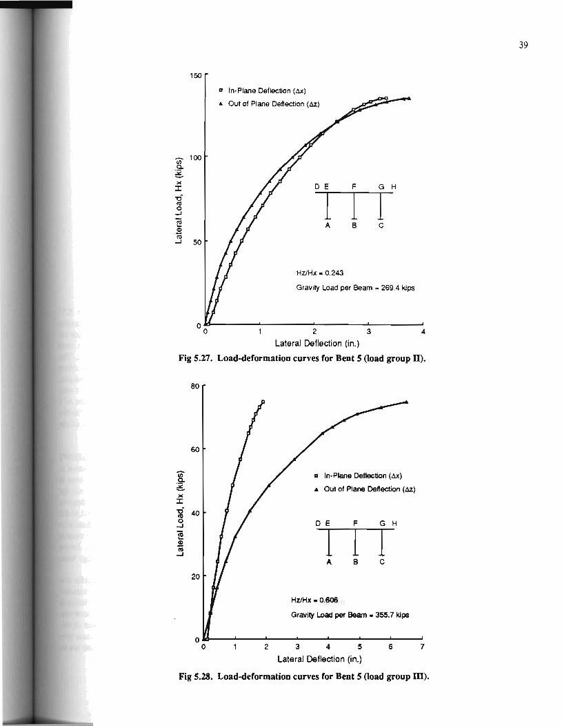
39

150

a In-Plane Deflection (<1X)

" Out of Plane Deflection (.:U)

(i) 100 ~

~ )(

D E F G H :I: -r;j I I I co 0

_..J

~ A B c Cl)

~ _..J 50

HZ/Hx • 0.243

Gravity Load per Beam ~ 269.4 kips

2 3 4

Lateral Deflection (in.)

Fig 5.27. Load-deformation curves for Bent 5 Ooad group II).

80

60

(i) a In-Plane Deflection (<1X) ~

~ • Out of Plane Deflection (.:U) )(

:I: '0 co 40 0 D E F G H ....J

iii I I I .... .S! co ....J

A B c

20

HZ/Hx • 0.606

Gravity Load per Beam. 355.7 kips

0 0 2 3 4 5 6 7

Lateral Deflection (in.)

Fig 5.28. Load-deformation curves for Bent 5 Ooad group ill).

40

TABLE 5.2. ULTIMATE LATERAL LOADS FOR BENTS

Ultimate Load Load

Bent Group Hx (kips) FaUure Mode

II 284.5 Tension Failure in Beam EF• m 212.4 Compression Failure in Column BF

2 II 303.0 Compression Failure in ColumnAE m 217.5 Compression Failure in Column CG

3 II 95.2 Compression Failure in Column EK m 69.6 Compression Failure in Column Cl

4 II 145.0 Compression Failure in Column CH m 24.9 Compression Failure in Column AF

5 II 133.5 Compression Failure in Column CG m 74.8 Compression Failure in Beam EF

• Members are indicated on corresponding figures.

combination I, the design moments were controlled by the minimum eccentricity criterion of the ACI code and are not presented here. Only one wind direction, perpendicular to the bridge longitudinal axis, is considered in computing the design wind loads (Table 5.1).

5.53.1 Bentl Figure 5.34 shows the variation of the inplane moments

with the applied inplane horizontal loads for load combina­tion II. The predicted in plane and out of plane moments for load group III are shown in Figures 5.35 and 5 .36. The design moments estimated by the ACI and TSDHPT procedures are also shown in these figures. It may be seen that for uniaxial bending under inplane loads (Fig 5.34), the results from all three analysis procedures are in good agreement. When the bent is subjected to biaxial lateral loads, the inplane mo­ments from the approximate and ACI methods are slightly higher (Fig 5.35) than the analytical predictions. The out of plane moments (Fig 5.36) calculated by the nonlinear analy­sis agree well with the results from the approximate proce­dure for low values of lateral loads (up to 50% of the predicted failure load). In the higher load range, the approxi­mate procedure underestimates the out of plane moments of the nonlinear analysis. The operating load ranges on the bridges are generally less than half of the ultimate loads (for a safety factor of 2.0). Thus it may be concluded that the moments computed by the approximate procedure are rea­sonable for service load conditions. The ACI method esti­mates out of plane moments greater than the analytical values. The difference between the out of plane moments from the ACI method and the nonlinear analysis reduces near failure of the structure. The difference between the failure loads of the three analysis procedures is within 10%.

5.5.3.2 Bent 2 The results for this bent are presented in Figs 5.37

through 5.39 for load groups II and III. The slenderness ratio of the bent is 36. Bents 1 and 2 are identical except for the number of girders on the bridge and their spacing. The trend of results for this bent is similar to the previous case. The ultimate lateral loads predicted by the analytical procedure agree well with the approximate and the ACI procedures. Again the TSDHPT procedure is in better agreement with the analysis results in the range of service loads than the ACI procedure. As loads increase toward failure the effective length factor (k) increases and the results approach of the ACI method.

5.5JJ Bent3 The moments from the nonlinear analysis, the TS DHPT

approximate procedure and the ACI method are shown in Figs 5.40 through 5.43. It may be noted that the bent is subjected to both inplane and out of plane lateral loads for load group n. The angle of skew for this bent is 30 degrees (Fig 5.5). As stated earlier, the skew angle is defined as the angle between the plane of the bent and the longitudinal axis of the bridge. The wind direction is considered as the normal to the bridge longitudinal axis. This resulted in forces parallel and perpendicular to the plane of the bridge bent. The column slendemess ratio for this bent is 46.4.

From Figs 5.40and 5.41, it may be observed that for low values of the lateral loads the approximate procedure under­estimates the analytical inplane moments. This deviation is due to the contribution of gravity loads on inplane moments. The approximate procedure neglects the moments devel­oped by the gravity loads. The out of plane moments pre­dicted by the approximate and nonlinear analyses are in

Cii Q.

;g. 1/) c: E :::3 0 (.)

.!: 1:J

"' 0 .....1

Cii

~

1/) Q.

~ 1/) c: E :::3 0 (.)

.E "'0

"' 0 .....1

iii ~

1600

a ColumnA D

• Column B

- TSDHPT 1200

BOO

D E F G H

I I I A B c

400

0._--------~--------~--------~--------~ 0 200 400 600

Gravity Load per Beam (kips)

Fig 5.29. Column axial forces for Bent 1 (load group 1).

1600

1200

BOO

400

a ColumnA

• Column B

- TSOHPT

0 E F

I I A B

G H

I c

200 400 600

Gravity Load per Beam (kips)

... ...

...

BOO

D

...

800

Fig 5.30. Column axial forces for Bent 2 (load group 1).

41

42

(i) .Q-6 f/) c: E ::1 0 (.)

c: "0 Ill 0

....J

~ )(

<(

(i) ~

~ f/) c: E ::1 0 (.)

.s; "0 Ill 0

....J

(ij

~

1600

a ColumnA

• Column B

Column C

- TSDHPT 1200

800

FG H J K L

400 I I I I I A B c D E

0~----~------~----~----~~----~----~ 0 100 200 300 400 500 600

Gravity Load per Beam (kips}

Fig 5.31. Column axial forces for Bent 3 (load group O.

1600

1200

800

400

a ColumnA

.a. Column B

- TSDHPT

E F

I A

G H

I I I B c D

0-------L----~~----._----~------~----~

J

0 100 200 300 400 500 600

Gravity Load per Beam (kips)

Fig 5.32. Column axial forces for Bent 4 (load group 1).

'[ ;g. (J)

1000

800

c 600 E :::1 0 (.)

.S: "0 <II .3 400 (ij ' )( <

200

0 0

Fig 5.33.

20000

15000 Vi' .9-~

~ N

::E 'E Cl) 10000 E 0

::E Cl) c <II a: .5

5000

0 0

a ColumnA

• Column B

• Column C

TSDHPT •

Cl

Cl

Cl

• Cl • •

• • D E F G H

• I I I • .. A B c

100 200 300 400 500

Gravity Load per Beam (kips)

Column axial forces for Bent 5 (load group 1).

Cl MA

• Me

• Me - TSDHPT

- ACI, MA

D E F G H

I I I A B c

Hz I Hx • 0

Gravity Load per Beam • 257.6 kips

50 100 150 200 250 300 350

Lateral Load, Hx (kips)

Fig 5.34. Column axial forces for Bent 1 (load group II).

43

44

1:1 MA 15000 • Me - TSDHPT - ACI, MA

Vi' a. ~ c: 10000 • N

::E c" • ~ D E F G 0

I I I ::E Ill c: I'll 5000 q: A 8 c .s

Hz/Hx • 0.45

Gravity Load per Beam - 344.4 kips

0 0 50 100 150 200

Lateral Load, Hx (kips)

Fig 5.35. Design moments for Bent 1 Ooad group ill).

15000

Ill .Q.. ~

~ )( 10000

::E

a MA

• Me

- TSOHPT

- ACI

H

250

0 E F G H

0 5000

'5 0

0 50

I I I A B c

Hz!Hx- 0.45

Gravity Load per Beam • 344.4 kips

100 150 200

Lateral Load, Hx (kips)

Fig 5.36. Design moments for Bent 1 (load group ill).

250

20000

en 15000 a. ~ c:

c <D 10000 E 0

:::E <D c: <ll a: .s

5000

a MA

• MC

- TSDHPT

- ACI,MA

D E F G H

I I I A B c

Hz/Hx- 0

Gravity Load per Beam - 289.0 kips

o~--------~----------~----------~----0 100 200 300

Lateral Load, Hx (kips)

Fig 5.37. Design moments for Bent 2 (load group 0).

a MA

15000 • Me ... TSDHPT - ACI,MA

en a. ~ g 10000

N :::E c: <D D E F G H E 0 I I I :::E <D c: <ll 5000 0:: A B c .s

Hz/Hx • 0.45

Gravity Load per Beam - 393.2 kips

0 0 50 100 150 200 250

Lateral Load, Hx (kips)

Fig 5.38. Design moments for Bent 2 Ooad gToup ill).

45

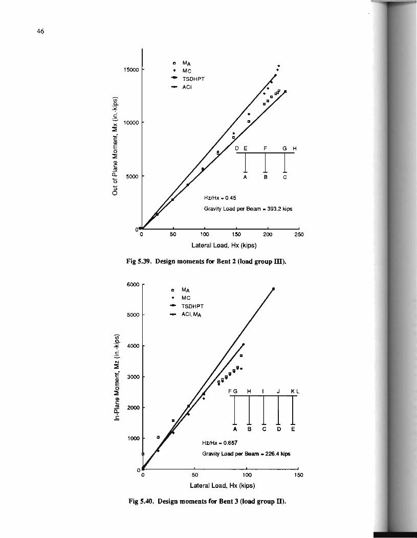
46

47

10000

II MA

• Me .... TSDHPT

8000 - ACI

til .9--'f ~ )(

::E 6000

c: Q)

E 0

::E Q) FG H J KL c: 4000

I I I I I ru a:: 0 5 0

2000 A 8 c D E

Hz/Hx • 0.657

Gravity Load per Beam - 226.4 kips

0 0 50 100 150

Lateral load, Hx {kips)

Fig 5.41. Design moments for Bent 3 (load group D).

6000 II MA

• MC -TSDHPT - ACI, MA 5000

FG H J KL til

I I I I I a. ~ 4000 ~ N ~ A 8 c D

-E ~ 3000

0 ~ Gl c: ru a:: 2000 .5

1000 Hz/Hx - 0.862

Gravity Load per Beam - 290.2 kips

0._----~----_.----~~----~----~----~ 0 20 40 60 80 100 120

Lateral load, Hx {kips)

Fig 5.42. Design moments for Bent 3 (load group ill).

48

10000

a MA

• Me - TSDHPT • a

8000 - ACI

(i) a. • ~ a

~ ~ )(

::E 6000

E CD E 0

::E (I)

4000 FG H J KL c: 11:1

I I I I I 0: 0 'S 0

2000 A B c D E

Hz/Hx • 0.862

Gravity Load per Beam - 290.2 kips

0 0 20 40 60 80 100 120

Lateral Load, Hx (kips)

Fig 5.43. Design moments for Bent 3 (load group ill).

close agreement up to 50% of the predicted failure load. The ACI method, however, overestimates the results for the out of plane moments. The difference between the results from the ACI method and the analytical procedure becomes smaller near failure of the structure. The failme loads from the ACI and analytical methods are in close agreement. The approximate procedure indicates a capacity of the bent (Hx= 126 kips) about 32% higher than the analytical capacity (Hx=95.2 kips). The results for group m loads are similar to those obtained for load combination II. The applied forces for load combinations II and III differ mainly in terms of the ratio of the out of plane to the inplane lateral loads (Hz/Hx) and the magnitude of gravity loads over the girders.

The load deflection curves for this bent (Figs 5.23 and 5.24) indicated a large increase in deflection prior to failure. Although the results showed a concrete compression failure, this sudden increase in deflection may be an indication of a stabilicy failure. The failure loads estimated by the ACI and the approximate procedures are based on the strength con­sideration. This may be the reason for higher ultimate lateral loads of the approximate procedures.

5.53.4 Btnt4 The slenderness ratio of this bent is 68,1arger than those

of the other four bents. The results for group IT loads obtained from the three analysis procedures are shown in Fig 5.44. In this case, the inplane moments from the ACI method agree reasonably well with the analytical moments. For a specified lateral load, the approximate procedure of TSDHPT esti­mates higher in plane moments than those obtained from the nonlinear analysis. The ultimate loads from the ACI method and the analytical procedure are the same. The approximate procedure indicates a capacity of the bent smaller than the nonlinear analysis predictions.

Figures 5.45 and 5.46 show the variation of the mo­ments for group III loads. The ACI method indicated insta­bilil)' of the system, as the applied gravicy load on columns is greater than the colwnn critical buckling load (out of plane direction). It may be seen that the inplane moments are reduced near the failure of the structure. This reduction is accompanied by a sudden increase in the out of plane moments. The load-deformation curves (Fig 5 .26) showed a sudden increase in deflection indicating instability

49

20000 a MA

• MB - TSDHPT - ACI, MA

15000 E F G H I J

Vl I I I I a. ~

c

N A B c ~

c: 10000 Cl)

E 0 ~ Cl) c Ill a: .5

5000

Hz/Hx- 0

Gravity Load per Beam - 302.0 kips

0 0 50 100 150

Lateral Load. Hx (kips)

Fig 5.44. Design moments for Bent 4 (load group II).

12000 a MA • Me - TSDHPT

10000

E F G H J Vl

I I I I a. ~ c:: 8000 --N A B c 0 ::E -E ~ 6000 0

::E ~ Ill 0: .s 4000

2000

Hz!Hx- 0.68

Gravity Load per Beam - 383.2 kips

0~----_.----~~----~----~----~----~ 0 10 20 30 40 50 60

Lateral Load, Hx (kips)

Fig 5.45. Design moments for Bent 4 Ooad group m).

50

20000 D MA E F G H I J

• MB I I I I - TSDHPT

A B c D (/) 15000 0. 3 ~ .£ )(

::E

'2 CD E 10000 0 ~ CD c ttl • 0::: 0 '5 0 5000

Hz/Hx • 0.68

Gravity Load per Beam • 383.2 kips

0~----~----~----_. ____ _. ____ ~~--~ 0 10 20 30 40 50 60

Lateral Load, Hx (kips)

Fig 5.46. Design moments for Bent 4 Ooad group ill).

failure.The approximate procedure overestimates the in­plane moments and underestimates the out of plane mo­ments compared with the analytical values. The failure load predicted by the approximate procedure (Hx=59.6 kips) is more than twice the analytical prediction (Hx=24.9 kips). This may again be attributed to the higher column slender­ness and instability failure mode.

5.53.5 Bent 5 The bent consists of girders positioned unsymmetri­

cally over the bent cap. The slenderness ratio of the bent columns is 44.8 and the skew angle is 14 degrees. The results for this bent are presented in Figs 5.47 through 5.50. For group II loads (Figs 5.4 7 and 5.48), the ultimate loads predicted by the three analysis procedures are in good agreement. As mentioned earlier, the approximate proce­dure neglects the inplane moments due to gravity loads. This may be the reason for the deviations between the inplane moments of the approximate and the analytical procedures. The effect is pronounced due to unsymmetrical arrangement of girders. The out of plane moments predicted by the approximate and the nonlinear analysis procedures are in excellent agreement up to 40% of the predicted failure load.

The inplane moments and ultimate loads predicted by the ACI method and the nonlinear analysis are within 10% for load combination III. The ACI method overestimates the

analytical results for the out of plane moments. The predic­tions of the approximate procedure are similar to the results for group II loads. The ultimate load predicted by the approximate procedure (Hx=l05 kips) is approximately 40% higher than the analytical predictions (Hx=74.8 kips). It may be noted that the structure failed due to crushing of concrete in the beam EF (Fig 5.49). From the variation of the out of plane moments, it is seen that the column was also on the verge of failure.

5.5.4 Effect of Slenderness Ratio of Bent Columns

In the previous section, the results for five bents were presented. These bents had different geometrical properties, layout and slenderness ratios. The objective of this section is to investigate the effect of slenderness ratio on the predicted behavior. Bent 2 of the previous section (Fig 5.3) was ana­lyzed with slenderness ratios of 40, 60 and 80. This was achieved by varying the length of the columns. The gravity load per beam was taken as 450 kips. A ratio of the out of plane lateral loads to inplane horizontal loads of 0. 75 was assumed. The results from the nonlinear analysis and the TSDHPT approximate procedures are discussed below.

5 5.4.1 Bents under Uniaxial Bending: The load-deflec­tion behavior of the bent for slenderness ratios of 40, 60 and 80 are shown in Fig 5.51. As expected, the lateral deflections

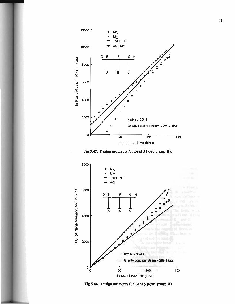
51

12000 tl MA

• Me - TSDHPT

10000 - Ael, Me

Ci) D E F G H

a. I I I ~ 8000 c ~

N A B e ::::E

c 6000

~ 0

::::E Q) c: ro a: 4000

.5

tl

2000 tl HzJHx • 0.243

tl Gravity Load per Beam • 269.4 kips

tl

0 0 50 100 150

Lateral Load, Hx (kips)

Fig 5.47. Design moments for Bent 5 (load group D).

8000

tl MA

• Me - TSDHPT - Ael

(/) 6000 .Q.. ~ D E F G H

~ I I I )(

~

E A B e

~ 4000 0 ~

~ ro

c::: 0 '5 0 2000

HZIHx - 0.243

Gravity Load per Beam- 269.4 kips

0 0 50 100 150

Lateral Load, Hx (kips)

Fig 5.48. Design moments for Bent 5 (load group m.

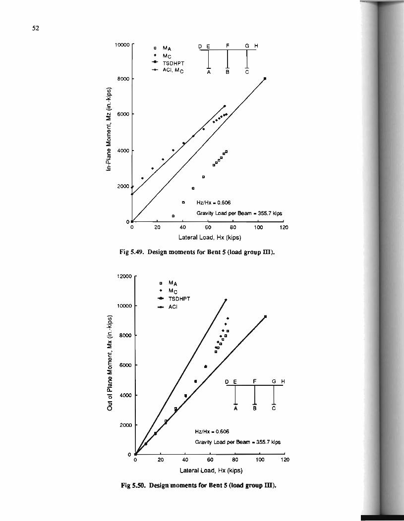
52

c" Q)

E 0

:::E

10000

8000

a MA

• Me ..... TSDHPT -+- Ael, Me

D E F G H

I I I A B e

~ 4000 r:P ra a: .5

(/)

.~

.lf

a

2000 a

a Hz/Hx • 0.606

a Gravity Load per Beam. 355.7 klps

0~----~----~----~----~----~----~ 0 20 40 60 80 100

Lateral Load, Hx (kips)

Fig 5.49. Design moments for Bent S (load group ill).

12000 a MA

• Me

- TSDHPT

10000 - Ael

120

£ 8000 )(

:::E

6000

D E F G H

4000 I I I A B e

2000 Hz/Hx • 0.606

Gravity Load per Beam. 355.7 klps

0 ~----~----~----~----~----~--~ 0 20 40 60 80 100 120

Lateral Load, Hx (kips)

Fig 5.50. Design moments for Bent 5 (load group ill).

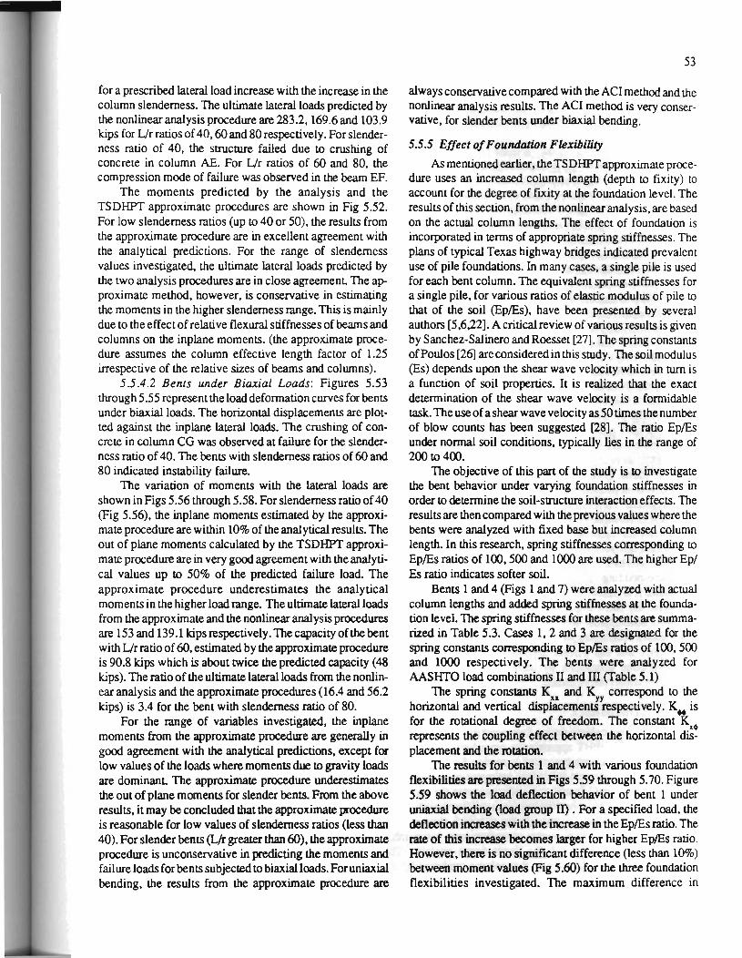
for a prescribed lateral load increase with the increase in the column slenderness. The ultimate lateral loads predicted by the nonlinear analysis procedure are 283.2, 169.6 and 103.9 kips for L/r ratios of 40, 60 and 80 respectively. For slender­ness ratio of 40, the structure failed due to crushing of concrete in column AE. For L/r ratios of 60 and 80, the compression mode of failure was observed in the beam EF.

The moments predicted by the analysis and the TSDHPT approximate procedures are shown in Fig 5.52. For low slenderness ratios (up to 40 or 50), the results from the approximate procedure are in excellent agreement with the analytical predictions. For the range of slenderness values investigated, the ultimate lateral loads predicted by the two analysis procedures are in close agreement The ap­proximate method, however, is conservative in estimating the moments in the higher slenderness range. This is mainly due to the effect of relative flexural stiffnesses of beams and columns on the inplane moments. (the approximate proce­dure assumes the column effective length factor of 1.25 irrespective of the relative sizes of beams and columns).

5.5 .4 .2 Bents under Biaxial Loads: Figures 5.53 through 5.55 represent the load deformation curves for bents under biaxial loads. The horizontal displacements are plot­ted against the inplane lateral loads. The crushing of con­crete in column CG was observed at failure for the slender­ness ratio of 40. The bents with slenderness ratios of 60 and 80 indicated instability failure.

The variation of moments with the lateral loads are shown in Figs 5.56 through 5.58. For slenderness ratio of 40 (Fig 5.56), the inplane moments estimated by the approxi­mate procedure are within 10% of the analytical results. The out of plane moments calculated by the TSDHPT approxi­mate procedure are in very good agreement with the analyti­cal values up to 50% of the predicted failure load. The approximate procedure underestimates the analytical moments in the higher load range. The ultimate lateral loads from the approximate and the nonlinear analysis procedures are 153 and 139.1 kips respectively. The capacity of the bent with L/r ratio of 60, estimated by the approximate procedure is 90.8 kips which is about twice the predicted capacity (48 kips). The ratio of the ultimate lateral loads from the nonlin­ear analysis and the approximate procedures (16.4 and 56.2 kips) is 3.4 for the bent with slenderness ratio of 80.

For the range of variables investigated, the inplane moments from the approximate procedure are generally in good agreement with the analytical predictions, except for low values of the loads where moments due to gravity loads are dominanL The approximate procedure underestimates the out of plane moments for slender bents. From the above results, it may be concluded that the approximate procedure is reasonable for low values of slenderness ratios (less than 40). For slender bents (L/r greater than 60), the approximate procedure is unconservative in predicting the moments and failure loads for bents subjected to biaxial loads. For uniaxial bending, the results from the approximate procedure are

53

always conservative compared with the ACI method and the nonlinear analysis results. The ACI method is very conser­vative, for slender bents under biaxial bending.

5.5.5 Effect of Foundation Flexibility

As mentioned earlier, the TSDHPT approximate proce­dure uses an increased column length (depth to fixity) to

account for the degree of fixity at the foundation level. The results of this section, from the nonlinear analysis, are based on the actual column lengths. The effect of foundation is incorporated in terms of appropriate spring stiffnesses. The plans of typical Texas highway bridges indicated prevalent use of pile foundations. In many cases, a single pile is used for each bent column. The equivalent spring stiffnesses for a single pile, for various ratios of elastic modulus of pile to that of the soil (Ep/Es), have been presented by several authors [5,6,22]. A critical review of various results is given by Sanchez-Salinero and Roesset [27]. The spring constants of Poulos [26] are considered in this study. The soil modulus (Es) depends upon the shear wave velocity which in tum is a function of soil properties. It is realized that the exact determination of the shear wave velocity is a formidable task. The use of a shear wave velocity as 50 times the number of blow counts has been suggested [28]. The ratio Ep/Es under nonnal soil conditions, typically lies in the range of 200 to400.

The objective of this part of the study is to investigate the bent behavior under varying foundation stiffnesses in order to determine the soil-structure interaction effects. The results are then compared with the previous values where the bents were analyzed with fixed base but increased column length. In this research, spring stiffnesses corresponding to Ep/Es ratios of 100, 500 and 1000 are used. The higher Ep/ Es ratio indicates softer soil.

Bents 1 and 4 (Figs 1 and 7) were analyzed with actual column lengths and added spring stiffnesses at the founda­tion level. The spring stiffnesses for these bents are summa­rized in Table 5.3. Cases 1, 2 and 3 are designated for the spring constants corresponding to Ep/Es ratios of 100, 500 and 1000 respectively. The bents were analyzed for AASIITO load combinations II and III (Table 5.1)

The spring constants K and K correspond to the horizontal and vertical disp~ement.frespectively. K~- is for the rotational degree of freedom. The constant K,. represents the coupling effect between the horizontal dis­placement and the rotation.

The results for bents 1 and 4 with various foundation flexibilities are presented in Figs 5.59 through 5.70. Figure 5.59 shows the load deflection behavior of bent 1 under uniaxial bending (load group m . For a specified load, the deflection increases with the increase in the Ep/Es ratio. The rate of this increase becomes larger for higher Ep/Es ratio. However, there is no significant difference (less than 10%) between moment values (Fig 5.60) for the three foundation flexibilities investigated. The maximum difference in

54

ultimate loads is less than 10% (Table 5.4). When the bent is subjected to biaxial loading, the trend of results (Figs 5.61 through 5.64) is somewhat similar to that for the uniaxial bending case.

Figure 5.65 shows the variation of the inplane horizon­tal deflection with the in plane lateral loads for bent 4 under uniaxial bending (load combination JD. The deflection val­ues for three cases of foundation flexibilities indicate a similar trend as observed for bent 1. The variation of in plane moments (Fig 5.66) indicates no difference in moment values for the three cases, except near failure of the structure. The difference between the ultimate loads for the three foundation flexibilities are within 10% (Table 5.4). When bent 4 is subjected to group III loads, a substantial reduction in ultimate loads is observed with the increase in Ep/Es ratio. The ratio of the ultimate lateral loads (Table 5.4) for cases 1 and 3 is 1.65. The load-deflection curves and the variation of the inplane and out of plane moments are presented in Figs 5.65 through 5.68. It may be noted that bent 4 experienced a large deflection before failure indicating an instability of the system. This may be one of the reasons for the drastic reduction in ultimate loads.

The previous two paragraphs summarized the results for bents 1 and 4 for three cases of foundation flexibilities. As stated earlier, the approximate procedure of the TSDHPT uses an increased column length to simulate the foundation conditions. This so called "depth to fixity" varies from 4 to 10 feet depending upon soil properties and engineering judgment The ultimate load predicted for bents 1 and 4 for various foundation flexibilities are shown in Table 5.4. The results for these bents obtained earlier are also included. Earlier analyses were based on an increased column length and fixed base. For bent 4 under biaxial bending, the values corresponding to Ep/Es ratio of 1000 show the best agree­ment It is observed that the bents with foundation springs generally show higher capacity and less deflections than their counterparts where the analysis is based on the in­creased column length. From these results, it may be con­cluded that the current approach of accounting for the foundation conditions by increasing the column length yields conservative results.

5.6 SUMMARY The bent column design forces and moments computed

using the TSDPHT approximate procedure and the linear frame analysis were presented in section 5.4. It was found that the approximate procedure estimates reasonably well the column axial forces and underestimates the moments (bent 1 through 4) when the live loads are distributed evenly between the beams. In one column of bent 5, the moments predicted by the approximate procedure were comparable with the moments from the linear frame analysis. The corresponding axial force in that column predicted by the

approximate procedure (load group II and III) was about half of the linear analysis value. However, in another column of bent 5, the axial load and moment were underestimated by the approximate procedure. The approximate procedure generally underestimates column axial forces and estimates moments reasonably well when the variation in the live load position is considered

The implications of the above results depend upon the criteria governing the design of bent columns. If the design is controlled by the axial strength of concrete then the high axial load and minimum moment constitute critical design forces. For this situation, the approximate procedure under­estimates the design axial forces (group I loads) when the variation in live load positions is considered. For group II and III loads, the higher moments and low axial loads predicted by the approximate procedure are conservative. An unconservative design situation (in the approximate procedure) was observed in a column of bent 5, where the moments from the two procedures were the same but the axial force from the approximate procedure was almost 50% of the linear frame analysis value. The results indicated that varying the live load positions on the deck has no significant influence compared with the live loads distributed equally between the beams for group III loads.

The results from the nonlinear analyses were compared with the values calculated by the ACI moment magnifier method and the TSDHPT approximate procedure (section 5.5). The load-deflection curves for various bents indicated higher out of plane deflections than the inplane deflections. This was explained in terms of cantilever action in the out of plane direction and the relative magnitude of lateral loads. The column axial forces (due to gravity loads on beams) calculated using the approximate procedure and the nonlin­ear analysis were in good agreement for bents 1 through 4. For bent 5, the nonlinear analysis showed scattering in column axial forces compared with the approximate analy-sis.

For bents under uniaxial bending (due to in plane lateral loads), inplane moments predicted by the three analysis procedures were generally in good agreement For low lateral loads, the inplane moments from the approximate procedure show some deviations from the nonlinear analysis results. This discrepancy appeared as the approximate pro­cedure neglects the effect of gravity loads on the inplane moments. The deviations in predicted moments were sub­stantial for bent 5 in which the girders were arranged unsymmetrically over the bent cap.

For bents mtder biaxial lateral loads, the inplane mo­ments calculated by the ACI method were in good agreement with the analytical moments. The ACI method overesti­mates the out of plane moments. The difference between the two results for out of plane moments become smaller near failure. The ultimate loads estimated by the ACI method

agree very well with the analytical predictions except for bent4. For bent4, the ACI approach was very conservative in predicting the failure load.

The results from the nonlinear analysis and the approxi­mate procedure indicated a good agreement for inplane moments. The out of plane moments from the two analysis procedures, for low to moderate slenderness ratios (less than 45), were in excellent agreement up to 50% of the predicted failure loads. For high lateral loads, the approximate proce­dure underestimates the analytical out of plane moments. For slender bents (Ljr greater than 60), the out of plane moments computed by the approximate procedure were smaller than those obtained from nonlinear analysis. The difference between the ultimate loads predicted by the approximate procedure and the nonlinear analysis were less than 20% for bents with slenderness ratio less than 45. For slender bents, the approximate procedure is unconservative in estimating the failure loads. It was found that the approxi­mate procedure reasonably estimates moments (both in­plane and out of plane) in bents with the column slenderness ratios (Ljr) less than 40.

The effect of foundation flexibility on the overall bent behavior was presented in section 5.5 .5. The load deflection curves indicated a higher rate of increase in deflection for

TABLE 5.3. EQUIVALENT SPRING STIFFNESS

Kxx Kyy KcMI Bent Case (lblio.) (lblio.) (in.-lb/rad) Kx~

.369"'10 7 .715•10 7 .854"'10 10 .111"'10 9

2 .212"'10 7 .406"'10 7 .653"'10 10 .711"'10 8

3 .554"'10 6 .978"'10 6 .451"'10 10 .321"'108

4 .307"'10 7 .594"'10 7 .496"'10 10 .773"'108

2 .177"'10 7 .338"'10 7 .379"'10 10 .494"'108

3 .503"'10 6 .815"'10 6 .262"'10 10 .223"'108

55

higher ratios of elastic moduli of pile and soil (Ep/Es). The difference between inplane moments for the three founda­tion flexibilities was less than 10% . For bent 1, the predicted out of plane moments for three foundation flexibilities were within 10%. However, bent 4 showed a drastic reduction in the out of plane moments with increasing Ep/Es ratio. The ultimate lateral loads predicted for three foundation condi­tions were essentially the same for bent 1 under uniaxial and biaxial bendings (load groups II and III) and bent 4 with inplane loads (load group II). The predicted ultimate load for bent4 for case 3 (Ep/Es=1000) was60% of the ultimate load corresponding to Ep/Es ratio of 100. The results for various foundation conditions were compared with the results where the degree of fixity at the foundation level is approximated by an increased column length and fixed base. For the range of variables investigated, it was concluded that the current approach of simulating the foundation condition is conser­vative.

TABLE 5.4. ULTIMATE LATERAL LOADS FOR BENTS

Wltb Without Load Springs Springs

Bent Group Case (kips) (kips)

II 1 341.0 284.5 2 331.0 3 308.7

m 1 273.3 212.4 2 270.7 3 254.8

4 II 1 165.2 145.0 2 163.5 3 153.0

m 1 39.1 24.9 2 34.5 3 23.7

56

300

Ur- 40

250

"iii a. 200 ~ >< :J: -o l1l 0 150 ...J

iii 'E 0 N ·;::

Ur-80 0 100 :J:

50

2 4 6 8 10 12 14

In-Plane Lateral Deflection, .1x (in.)

Fig 5.51. Load-denection curves for Bent 2 with various slenderness ratios (uniaxial bending).

"iii a. ~ .g 'E ~ 0 ~ Q) c: l1l a: ..s

20000

15000

10000

5000

TSDHPT Approximate Method

ur -so a

Ur -40

D E F G H

I I I A B c

HZ/Hx. 0

Gravity Load per Beam - 450 kips

0 ~---------------~---------------~------------~ 0 100 200 300

Horizontal Load, Hx (kips)

Fig 5.52. lnplane moments for Bent 2 (M.._) with various slenderness ratios (uniaxial bending).

57

160

120

"ii) 0.

~ )(

I -o - In-Plane Deflection (6X) I'll 80 0 - Out of Plane Deflection (6.Z) -1

Iii c 0 .!::i .... 0 I Hz/Hx • 0.75

40 Gravity Load per Beam - 450 kips

04---------L-______ _. ________ ~------~

0 2 4 6 8

Lateral Displacement (in.)

Fig 5.53. Load versus displacement for Bent 2 under biaxial bending (Ur = 40).

60 - In-Plane Deflection (6X)

- Out of Plane Deflection (6.Z)

50

"ii) 0.

40 ~ )(

I -o I'll 0 30 -1

Iii c 0 N ·.::: 0 20 I

10 Hz!Hx • 0.75

Gravity Load per Beam • 450 kips

o~----~------._ ____ ~ ______ ._ ____ ~ 0 2 4 6 8 10

Lateral Deflection (in.)

Fig 5.54. Load versus displacement ror Bent 2 under biaxial bending (Ur = 60).

58

20

- In-Plane Deflection (6X)

- Out of Plane Deflection (62:)

15

(j) .Q-6 X

I -o Ill 0 -l 10

Ill c: 0 N ·;:: 0 I

5

HZ/Hx • 0.75

Gravity Load per Beam - 450 kips

0 0 2 3 4 5 6

Lateral Deflection (in.)

Fig S.SS. Load versus displacement for Bent 2 under biaxial bending (IJr = 80).

20000 a Out of Plane Moment at A

• Out of Plane Moment at C

• In-Plane Moment at A • • In-Plane Moment at C .. - TSDHPT. Mx

• a 15000 -TSDHPT, Mz a

.. a

D E F G H a • (j) I I I a. ~ c:

10000 A B c c: Q)

E 0 ~

5000

HZ!Hx • 0.75

Gravity Load per Beam - 450 kips

0~------~--------~--------~------~ 0 40 80 120 160

Lateral Load, Hx (kips)

Fig 5.56. Design moments for Bent 2 under biaxial bending (Ur = 40).

59

20000 a Out of Plane Moment at A ... Out of Plane Moment at C

• In-Plane Moment at A

• In-Plane Moment at C - TSDHPT, Mx 16000 -a- TSDHPT, Mz

... (i) a_

12000 ~ ... . s ... c a> E 0 8000 :::E

E F G H

4000 I I I A 8 c

HZ/Hx- 0.75

Gravity Load per Beam - 450 kips

0 0 20 40 60 80 100

Lateral Load, Hx (kips)

Fig 5.57. Design moments ror Bent 2 under biaxial bending (L/r = 60).

16000 a Out of Plane Moment at A

... Out of Plane Moment at C

• In-Plane Moment at A

• In-Plane Moment at C

- TSDHPT, Mx 12000 - TSDHPT; Mz

(i) a_

~ g

8000 c ... ~ ... 0 ~

E F G H

4000 I I I A B c

HZ!Hx- 0.75

Gravity Load per Beam - 450 kips

0 m-~~._----~----~----~----~----~ 0 10 20 30 40 50 60

Lateral Load, Hx (kips)

Fig 5.58. Design moments ror Bent 2 under biaxial bending (Ur = 80).

60

400 - Case 1 (Ep/Es- 100) - Case 2 (Ep/Es - 500) - Case 3 (Ep/Es. 1000)

300

en a. ~ >< :I: -o co 0

200 ....J

rn c: 0

.~ ..... 0 :I:

100

Hz I Hx • 0

Gravity Load per Beam - 257.6 kips

0 0 2 3 4

In-Plane Horizontal Deflection, L1X (in.)

Fig 5.59. Effect of foundation nexibility on lateral denection (Bent 1 under Group n loads).

20000 Moments at B

a Case 1 (Ep/Es- 100) a a

• Case 2 (Ep/Es • 500) f • Case 3 (Ep/Es. 1000) 8 16000

en .. a. • ~ 8.

~ • N 12000 ~ a • E • ~ ~ 0 ~ • Q) 8000 c: 8 D E F G H "' a: • I I I ' .£ 8

• A B c 4000 8

• Hz/Hx • 0

I Gravity Load per Beam - 257.6 kips

0 0 100 200 300 400

In-Plane Lateral Load, Hx (kips)

Fig 5.60. Effect of foundation nexibility on design moment (Bent 1 under Group D loads).

300 - Case 1 (Ep/Es • 100) - Case 2 (EpiEs • 500) - Case 3 (Ep/Es. 1000)

250

Vi" .9-c. X 200 :I: -o ~ 0

..J c;;

150 c: 0 N ·;:: 0 :I: a> c: 100 ~

a: £

50 HZ/Hx. 0.45

Gravity Load per Beam • 344.4 kips

0 ~------~---------L--------~------~ 0 2 3 4

In-Plane Lateral Deflection, ~x (in.)

Fig 5.61. Effect or foundation flexibility on inplane deflection (Bent 1 under Group ill loads).

Vi" Q.

~ )(

:I: "0 ~ 0 ..J

ii .... a> j a> c: t1S a: £

300

200

100

A. Case 1 (Ep/Es. 100)

- Case 2 (Ep/Es - 500)

- Case 3 (Ep/Es- 1000)

HZ!Hx-0.45

Gravity Load per Beam- 344.4 klps

o._------~----_.------~------~----~ 0 1 2 3 4 5

Out of Plane Horizontal Deflection, tJ.Z. (in.)

Fig 5.62. Effect or foundation flexibility on out of plane def1ection (Bent 1 under Group m loads).

61

62

16000 Moments at B

a Case 1 (Ep/Es • 100)

• Case 2 (Ep/Es - 500)

• Case 3 (Ep/Es- 1000) r/

12000 v. Ul Q. • ~ ~ v

• N ::::E 2 i'

8000 • Q) a E • 0 • ::::E a • Q) c a • D E F G H ns a: •

I I I .5: a • • 4000 • v A B c •

8 Hz/Hx • 0.45 •

I Gravity Load per Beam - 344.4 kips

0 0 100 200 300

In-Plane Horizontal Load, Hx (kips)

Fig 5.63. Effect or foundation nexibility on inplane moment (Bent 1 under Group m loads).

16000 Moments at B

a Case 1 (Ep/Es- 100)

• Case 2 (Ep/Es - 500) • a• • Case 3 (Ep/Es- 1000)

• In 12000 a .Q.. -¥ • ~ a >< • ::::E 8 c • ~ 8000 • 0

::::E • • ~ ns • F G a: • D E H

0 I I I I 5 0 4000

I A B c I Hz!Hx- 0.45

I Gravity Load per Beam • 344.4 kips

0 0 100 200 300

In-Plane Lateral Load, Hx (kips)

Fig 5.64. Effect or foundation nexibility on out or plane moment (Bent 1 under Group m loads).

63

200 - Case 1 (EpiEs • 100) - Case 2 (EpiEs • 500) - Case 3 (EpiEs s 1000)

160

VI a. 6 )(

J: -o 111

120 0

...J !ij .... cp iV ...J cp c 80 111 ~ £

40

Hz/Hx. 0

Gravity Load per Beam - 302 kips

0~----~--~----~----~----_.----~ 0 2 4 6 8 10 12

In-Plane Horizontal Deflection, t:.x (in.)

Fig 5.65. Effect of foundation flexibility on lateral deflection (Bent 4 under Group D loads).

20000 Moments at B

a Case 1 (EpiEs - 100)

• Case 2 (EpiEs - 500)

• Case 3 (EpiEs • 1000) 16000

(i) E F G H J a a.

I I I I • • ~ . S •• "' 12000

A B c D • ~ • c: • • cp • E • 0 ~

8000 • cp I c

111 ~ .s I

4000 I

Hz/Hx- 0

I Gravity Load per Beam • 302 klps

0 0 40 80 120 160 200

In-Plane Horizontal Load, Hx (kips)

Fig 5.66. Effect of foundation flexibility on design moment (Bent 4 under Group n loads).

64

40

U) 30 a. ~ )(

:::z:::

"'0 rD 0

....J

~ 20 G)

ii'i ....J G) c:: rD a: £

10

- Case 1 (EpiEs - 100)

- Case 2 (EpiEs - 500)

- Case 3 (EpiEs- 1000)

HZ/Hx- 0.68

Gravity Load per Beam - 383.2 kips

0~~----~--------~-------L------~ 0.0 0.5 1.0 1 .5 2.0

In-Plane Horizontal Deflection, .1.X (in.)

Fig 5.67. Effect of foundation nuibiJity on inplane denection (Bent 4 under Group ill loads).

40

- Case 1 (EpiEs- 100)

- Case 2 (EpiEs • 500)

- Case 3 (EpiEs- 1000) 10

HZIHx • 0.68

Gravity Load per Beam. 383.2 kips

0~----~------~---------~~---L----~ 0 4 8 12 16 20

Out of Plane Horizontal Deflection, t:.z (in.)

Fig 5.68. Effect of foundation nuibUity on out of plane denection (Bent 4 under Group ill loads).

3000

Moments at B a a

a a Case 1 (EpiEs- 100) a

a a • Case 2 (EpiEs - 500) • • Case 3 (EpiEs- 1000)

a • • 2000

a • •

a • •

a • • E F G H J 1000 I I I I g

• A B c D

I Hz/Hx • 0.68

Gravity Load pet" Beam - 383.2 kips

0 0 10 20 30 40

In-Plane Lateral Load, Hx (in.)

Fig 5.69. Effect or foundation nexibility on inplane moment (Bent 4 under Group m loads).

i ~ ~ )(

~

E ~ 0 ~

! co a: 0 s 0

20000

16000

12000

8000

4000

Moments at B (See Figure 5.69)

a Case 1 (EpiEs- 100)

• Case 2 (EpiEs - 500)

• Case 3 (EpiEs • 1 000)

• •

• • a

•

• a

Hz!Hx • 0.68

• a

• a

• • Gravity Load pet" Beam - 383.2 kips

0 L-------~--------~--------~------~ 0 10 20 30 40

In-Plane Lateral Load, Hx (kips)

Fig S. 70. Effect of foundation nexibUity on out of plane moment (Bent 1 under Group m loads).

65

CHAPTER 6. CONCLUSIONS AND RECOMMENDATIONS

6.1 SUMMARY OF THE STUDY The objective of this research was to evaluate the

accuracy and suitability of the current office procedure of the Texas State Department of Highways and Public Transpor­tation (TSDHP1) for designing slender bent columns. The study involved developing two computer programs. The linear frame analysis program was developed to evaluate the design forces considering the total gravity load on the bridge divided equally between the girders. The variation in the positions of live loads was also included in the analysis. The moment magnifier method of AASHTO was used to ap­proximate second order effects. The design forces from the linear frame analysis were compared with those obtained from the TSDHPT approximate procedure.

The nonlinear method of analysis, developed in this research, was used to predict the three dimensional behavior of slender reinforced concrete bridge bents. The fiber model and an updated Lagrange finite element formulation were used to model the geometric and material nonlinearities. A variety of problems were solved to determine the accuracy and efficiency of the proposed formulation. The behavior of a number of typical bridge bents was studied. The results from the nonlinear analysis were compared with the predic­tions of the TSDHPT approximate procedure and the AASHTO moment magnifier method. The sensitivity of the results to column slenderness and foundation flexibilities were evaluated in terms of the predicted bent behavior.

6.2 CONCLUSIONS

6.2.1 Appro:rimDte Procedure vs Linear Franu ANJlysis

Comparison of results from the linear frame analysis and the approximate procedure indicated that the current office procedure generally underestimares column axial forces and overestimates associated bending moments in typical highway bridge bents. For AASHTO load combina­tion I, the approximate procedure results in axial forces which are smaller than the real ones. 1be design of bent columns, in this load group, is governed by high axial load and low bending moment For group ll and ill loads, how­ever, the approximate procedure estimates reasonably the design forces for typical bent geometries (bents 1 through 4 ). As the bent geometry deviates from the typical ones, the uncertainty related to the approximate method increases. In some cases (bent 5), the approximate method estimates unconservative design forces compared with the linear frame analysis values. It was found that varying the position of live loads over the deck does not drastically change the

66

design forces for load group ill although it is a major factor in the discrepancies for load group I.

6.2.2 Appro:rimtlte Procedure vs Nonlinear Analysis

The results from the approximate procedure, the AASHTO moment magnifier method and the nonlinear analysis were compared for slender bents under both uniax­ial and biaxial lateral loads. For the range of values investi­gated, the following conclusions were reached:

( 1) For bents under in plane lateral loads (uniaxial bend­ing) and with column slenderness ratios (L/r) less than 50, the moments predicted by the approximate procedure are in good agreement with the analytical values, except for low values of lateral loads (in some cases). This deviation is due to the exclusion of moments developed by gravity loads in the approximate procedure. The failure load predicted by the office procedure was in good agreement with the analytical predictions. For slender bents (say L/r > 60), the approxi­mate procedure is conservative in predicting the analytical failure load. The results from the moment magnifier method and nonlinear analysis were in very good agreement for the range of slenderness values investigated.

(2) For bents under biaxial bending, the inplane mo­ments predicted from the nonlinear analysis and approxi­mate procedures were in good agreement except for low values of loads where gravity load moments are dominant. For bents with low to moderate slenderness ratios (L/r < 40), the out of plane moments. from the approximate procedure and the nonlinear analysis were in excellent agreement up to 50% of the predicted failure load. For higher loads, the approximate procedure underestimates the analytical out of plane moments. The failure loads predicted by the two procedures are within 20%. The inplane moments and fail­ure loads estimated by the AASHTO moment magnifier method were in good agreement with the analytical predic­tions. The moment magnifier method overestimates the analytical out of plane moments. The difference reduces near the failure of the structure.

(3) For slender bents (J..Jr > 60) under biaxial bending, the approximate procedure overpredicts the analytical ulti­mate la1eralloads. The out of plane moments predicted by the approximate procedure are smaller than the analytical predictions for slender bents. The ACI procedure is very conservative in estimating the failure load for slender bents.

( 4) Comparison of results for various foundation flexi­bilities and the current procedure of assuming fixity depth indicated that the current approach yields conservative re­sults for typical Texas soil conditions.

6.3 RECOMMENDATIONS For the range of variables examined, it seems appropri­

aae to use the current office procedure for designing typical bridge bent columns of slenderness ratio (Ur) less than 40. For slender bents (Ur > 60), the designers are cautioned against the use of the current office procedure. The values of effective length factor need to be critically examined. In the absence of a more sophisticated analysis tool, like the nonlinear analysis program developed in this study, the use of the AASHTO moment magnifier method is recom­mended although it gives very conservative design values especially for slender bents.

67

6J.l Research Needs

Several research areas in which additional work is needed are:

- Study of multi-story bents underbiaxiallateralloads. - Study of bents with different column cross sections,

e.g. hollow shaft, hollow rectangular sections. - Study of bents with high strength materials. -Parametric study of heavily loaded slender bents

(bridge spans >100 feet).

REFERENCES 1. ACI Committee 318, Building Code Requirement for 15. Furlong, R. W., "Column Slenderness and Charts for

Reinforced Concrete (ACI 318-83), American Design," ACI Journal, Proceedings, Vol 68, No. Concrete lnstiblte, Detroit, 1983. 1, January 1971, pp 9-17.

2. ACI Committee 318, Commentary on Building Code 16. Hognestad, E., "A Sbldy of Combined Bending and Requirement for Reinforced Concrete (ACI 318- Axial Load in Reinforced Concrete Members," 83), American Concrete Institute, Detroit, 1983. University of Illinois Bulletin, Engineering Ex-

3. Adams, John, "Nonlinear Behavior of S tee I Frames," perimentaJ Station Bulletin Series No. 399, No-

unpublished Ph. D. dissertation, Massachusetts vembet 1951.

Institute of Technology, 1973. 17. MacGregor, J. G., and Hage, S. E., "Stability Analysis

4. American Association of State Highway and Trans- and Design of Concrete Frames," Journal of the

portation Officials, Standard Specifications for Structural Division, ASCE, Vol 103, No. STlO,

Highway Bridges, 12th Edition, 1977. October 1977, pp 1953-1970.

5. Blaney, G. W., Kausel, E., and Roesset, J. M., "Dy- 18. MacGregor, J. G., Breen, J. E., and Pfrang, E. 0.,

namic Stiffness of Piles," Proceedings, 2nd Inti. "Design of Slender Concrete Columns," Journal of

Conf. Num. Meth. Geomechanics, ASCE, pp the American Concrete Institute, Proceedings, Vol

1001-1012. 67, No. 1, January 1970, pp 6-28.

6. Breen, J. E., MacGregor, J. S., and Pfrang, E. 0., 19. Newmark, N. M., "Numerical Procedure forComput-

"Determination of Effective Length Factor for ing Deflections, Moments, and Buckling Loads,"

Slender Concrete Columns," ACI Journal, Vol69, Transactions, ASCE, Vol108, 1943, p 1161.

No. 11, November 1972, pp 669-672. 20. Newmark, N. M., and Rosenbleuth, E., Fundamentals

7. Chen, W. F.,andAtsuta, T., TheoryofBeam-Columns, of Earthql4tlU Enginuring, Prentice-Hall, Inc.,

Vol2, McGraw-Hill, 1977. 1971.

8. Clough, R. W., and Penzien, J., Dynamics of Struc- 21. Nixon, D., Beaulieu, D., and Adams, P. F., "Simplified

tures, McGraw-Hill, 1975. Second-Order Frame Analysis," Canadian Journal

9. Cook, R. D., Concepts and Applications of Finile of Civil Engineering, Voi2,No.4, December 1975,

Element Analysis, John Wiley & Sons, Inc., 1974. pp 602-605.

10. Diaz, M.A., "Evaluation of Approximate Slenderness 22. Novak, M., "Dynamic Stiffness and Damping of

Procedures for Nonlinear Analysis of Concrete and Piles," Canadian Geotechnical Journal, Vol 11,

Steel Frames," Ph.D. Disseratation, The Univer-No.4, 1974, pp 574-598.

sity of Texas at Austin, December 1984. 23. Poston, R. W., "Computer Analysis of Slender

11. Ernst, C., Smith, M., Riveland, R., and Pierce, N., Nonprismatic and Hollow Bridge Piers," M.S.

"Basic Reinforced Concrete Frame Performance Thesis, The University of Texas at Austin, Texas,

Under Vertical and Lateral Loads," ACI Journal, May 1980.

Proceedings, Vol 70, No.4, April1973, pp 261- 24. Poston, R. W., Breen, J. E., Roesset, J. M., "Analysis

269. of Nonprismatic or Hollow Slender Concrete

12. Farah, A., and Huggins, M. W., "Analysis of Rein-Bridge Piers," ACIJ oumal, Vol82, No. 5, Septem-

forced Concrete Columns Subjected to Longitudi-bet-October 1985, pp 731-739.

naiLoadsandBiaxialBending," ACI Journai,July 25. Poston, R. W., Diaz, M., Breen, J. E., and Roesset,

1969, pp 569-575. J. M., "Design of Slender, Non prismatic, and

13. Ferguson, P.M., and Breen, J. E., "Investigation of the Hollow Concrete Bridge Piers," Research Report

Long Concrete Column in a Frame Subject to 254-2F, Center for Transportation Research, The

Lateral Loads," Symposium on Reinforced Con-University of Texas at Austin, August 1982.

crete Columns, SP-13, American Concrete lnsti- 26. Poulos, H. G., "Behavior of Laterally Loaded Piles: I

tute, Detroit, 1966, pp 75-120. - Single Piles," Journal of Soil Mechanics and

14. Ford, J. S., Chang, D. C., and Breen. J. E., "Design Foundations Division, ASCE, Vol 97, No. SM5,

Indications from Tests of Unbraced Multipanel 1971, pp 711-731.

Concrete Frames," Concrete International, March 1981, Vol 103, No.3, pp 3747.

68

27. Sanchez-Salinero, I., and Roesset. J. M., "Static and Dynamic Stiffnesses of Single Piles," Geotechni­cal Engineering Report GR82-31, Geotechnical Engineering Center, Civil Engineering Depart­ment. The University of Texas at Austin, August 1982.

28. Schmertmann, J. H., "Use of lhe SPT lO Measure Dynamic Soil Properties?- Yes, But..!,"Dynamic Georeclmical Testing, ASTM, STP 654, 1978.

29. Stocks, R. W., "Computer Program f<X' the Analysis of Bridge Bent Columns Including a Graphical Interface," M.S. Thesis, The University of Texas at Austin, December 1987.

30. Sykora.D. W .• ''ExaminationofExistingShearWave Velocity and Shear Modulus Correlations in

69

Soils," Report. Department of lhe Army, Water­ways Experimental Station, C{X'ps of Engineers. Mississippi, September 1987.

31. Veletsos, A. S., and Wei, Y. T., "Lateral and Rocking Vibration of Footings," ASCE Soil Mechanics Journal, Vol 97, No. SM9, September 1971, p 1227.

32. Wood. B. R., Beaulieu, D., Adams, P. F., "Column Design by P-Delta Method," Journal of lhe Struc­tural Division, ASCE, Voll02, No. ST2, February 1976, pp 411-427.

33. Wood, B. R., Beaulieu, D., Adams, P. F., "Further Aspects of Design by P-Delta Model," Journal of the Structural Division, ASCE, Voll02, No. ST3. March 1976, pp 487-500.