analysis and comparison of separation measurement … · prepared for the federal aviation...
TRANSCRIPT

Report No. DOT/FAA/RD-95/5
ProjectReport
ATC-306
LincolnLaboratoryMASSACHUSETTS INSTITUTE OF TECHNOLOGY
LEXINGTON, MASSACHUSETTS
21 October 2002
S.D. Thompson
PreparedfortheFederalAviationAdministration.
DocumentisavailabletothepublicthroughtheNationalTechnicalInformationService,
Springfield,Virginia22161.
AnalysisandComparisonofSeparationMeasurementErrorsinSingleSensorandMultiple
RadarMosaicDisplayTerminalEnvironments

This document is disseminated under the sponsorship of the Department of Transportation in the interest of information exchange. The United States Government assumes no liability for its contents or use thereof.

1. Report No. 2. Government Accession No. 3. Recipient's Catalog No.
ATC-306
4. Title and Subtitle 5. Report Date
Analysis and Comparison of Separation Measurement Errors in Single 21 October 2002Sensor and Multiple Radar Mosaic Display Terminal Environments 6. Performing Organization Code
7. Author(s) 8. Performing Organization Report No.
S. D. Thompson ATC-3069. Performing Organization Name and Address 10. Work Unit No.
MIT Lincoln Laboratory244 Wood Street
11. Contract or Grant No.
Lexington, MA 02420-910812. Sponsoring Agency Name and Address 13. Type of Report and Period Covered
Department of TransportationProject ReportFederal Aviation Administration
Washington, DC 2059114. Sponsoring Agency Code
15. Supplementary Notes
This report is based on studies performed at Lincoln Laboratory, a center for research operated by MassachusettsInstitute of Technology under Air Force Contract FI9628-00-C-0002.
16. Abstract
This paper presents an analysis to estimate and characterize the errors in the measured separation distance betweenaircraft that are displayed on a radar screen to a controller in a single sensor terminal environment compared to amultiple radar mosaic terminal environment. The error in measured or displayed separation is the difference betweenthe true separation or distance between aircraft in the air and the separation displayed to a controller on a radar screen.In order to eliminate as many variables as possible and to concentrate specifically on the differences between displayedseparation errors in the two environments, for the purposes of this analysis, only full operation Mode S secondarybeacon surveillance characteristics are considered. A summary of the Mode S secondary radar error sources andcharacteristics used to model the resultant errors in measured separation between aircraft in single and multi-radarterminal environments is presented. The analysis for average separation errors show that the performance of radars inproviding separation services degrades with range. The analysis also shows that when using independent radars in amosaic display, separation errors will increase, on average, compared to the performance when providing separationwith a single radar. The data presented in the section on average separation errors is summarized by plotting thestandard deviation of the separation error as a function of range for the single radar case and for the independentmosaic display case. The sections on typical and specific errors in separation measurements illustrate that theseparation measurement errors are highly dependent on the geometry of the aircraft and radars. Applying averageresults to specific geometries can lead to counter intuitive results is illustrated in an example case presented in analysis.
17. Key Words 18. Distribution Statement
Air traffic control, aircraft separation standards, radar separation errors This document is available to the publicthrough the National TechnicalInformation Service, Springfield, VA22161
19. Security Classif. (of this report) 20. Security Classif. (of this page) 21. No of Pages 22. Price
Unclassified Unclassified 112
Form DOT F 1700.7 (8-72) Reproduction of completed page authorized

ABSTRACT
This paper presents an analysis to estimate and characterize the errors in the measured separationdistance between aircraft that are displayed on a radar screen to a controller in a single sensor terminalenvironment compared to a multiple radar mosaic terminal environment. The error in measured ordisplayed separation is the difference between the true separation or distance between aircraft in the airand the separation displayed to a controller on a radar screen. In order to eliminate as many variables aspossible and to concentrate specifically on the differences between displayed separation errors in the twoenvironments, for the purposes of this analysis, only full operation Mode S secondary beacon surveillancecharacteristics are considered. A summary of the Mode S secondary radar error sources andcharacteristics used to model the resultant errors in measured separation between aircraft in single andmulti-radar terminal environments is presented. The analysis for average separation errors show that theperformance of radars in providing separation services degrades with range. The analysis also shows thatwhen using independent radars in a mosaic display, separation errors will increase, on average, comparedto the performance when providing separation with a single radar. The data presented in the section onaverage separation errors is summarized by plotting the standard deviation of the separation error as afunction of range for the single radar case and for the independent mosaic display case. The sections ontypical and specific errors in separation measurements illustrate that the separation measurement errorsare highly dependent on the geometry of the aircraft and radars. Applying average results to specificgeometries can lead to counter intuitive results is illustrated in an example case presented in analysis.
iii

TABLE OF CONTENTS
Abstract
List of Illustrations
I. INTRODUCTION
111
VII
2.
3.
4.
5.
MODE S RADAR ERRORS
2.1 Radar Site Location Bias
2.2 Range Errors2.3 Azimuth Errors
2.4 Errors In Displayed Separation Due To Timing2.5 Performance Metric
SEPARATION MEASUREMENT ERROR ANALYSIS
3.1 Average Separation Errors3.2 Typical Separation Error Characteristics3.3 Separation Errors for Specific Simulation Cases
SIMULATION PROCEDURES
4.1 Average errors in Separation Measurements, One Radar
4.2 Average Errors in Separation Measurements, Two Radars
4.3 Typical Errors in Separation Measurement4.4 Specific Errors in Displayed Separation
RESULTS
5.1 Average Errors in Separation Estimates5.2 Typical Errors in Separation Measurements5.3 Specific Measurements
3
34
6
810
11
111314
17
17181920
23
234064
6. SUMMARY AND CONCLUSIONS
7. REFERENCES
A. APPENDIX, MATLAB SIMULATION PROCEDURES AND SCRIPTS
A.1 Average Errors in Separation Measurements, One RadarA.2 Average Errors in Separation Measurements, Two RadarsA.3 Typical Errors in Separation Measurement
A.4 Specific Errors in Displayed Separation
v
75
79
81
818590
100

FigureNo.
1
2
3
4
5
6
7
8
9
10
11
12
13
14
15
16
17
18
19
20
21
22
23
24
LIST OF ILLUSTRATIONS
PageNo.
Location Bias 3
Illustration of the magnitude of the range error sources 5
Illustration of the magnitude of the azimuth error sources at a range of 30 nautical miles 7
Illustration of the effect of clock bias on separation measurement 9
Average performance measurement statistics were generated by placing the midpoint of aircraftthree nautical miles in-trail at specified ranges and randomly orienting the aircrafts'paths about <p 12
Typical errors in estimating aircraft separation were measured for specified radar and aircraftgeometries. Bias errors were sampled once; jitter errors were sampled for each simulation 13
Separation measurement performance for specific cases use specified radar locations and aircraftflight paths to simulate errors for each individual position measurement 14
Average separation estimates for a single radar at a 5 nmi range 24
Average separation estimates for a single radar at a 10 nmi range 25
Average separation estimates for a single radar at a 20 nmi range 26
Average separation estimates for a single radar at a 30 nmi range 27
Average separation estimates for a single radar at a 40 nmi range 28
Average separation estimates for a single radar at a 50 nmi range 29
Average separation estimates for a single radar at a 60 nmi range 30
Average separation estimates for independent radars at 5 mni Range, e =0° 31
Average separation estimates for independent radars at 10 nmi Range, e =0° 32
Average separation estimates for independent radars at 20 nmi Range, e =0° 33
Average separation estimates for independent radars at 30 nmi Range, e =0° 34
Average separation estimates for independent radars at 30 nmi Range, e =30° 35
Average separation estimates for independent radars at 30 nmi Range, e =45° 36
Average separation estimates for independent radars at 40 nmi Range, e =0° 37
Average separation estimates for independent radars at 50 nmi Range, e =0° 38
Average separation estimates for independent radars at 60 nmi Range, e =0° 39
Radar and aircraft geometry for Case 1 41
Vll

LIST OF ILLUSTRATIONS (Continued)
25 Typical separation estimates for radar I, Case 1 42
26 Typical separation estimates for radar 2, Case 1 43
27 Typical separation estimates independent radars, Case 1 44
28 Radar and aircraft geometry for Case 2 45
29 Typical separation estimates for radar 1, Case 2 46
30 Typical separation estimates for radar 2, Case 2 47
31 Typical separation estimates independent radars, Case 2 48
32 Typical separation estimates additional case of independent radars, Case 2 49
33 Radar and aircraft geometry for Case 3 50
34 Typical separation estimates for radar I, Case 3 51
35 Typical separation estimates for radar 2, Case 3 52
36 Typical separation estimates independent radars, Case 3 53
37 Radar and aircraft geometry for Case 4 54
38 Typical separation estimates for radar I, Case 4 55
39 Typical separation estimates for radar 2, Case 4 56
40 Typical separation estimates independent radars, Case 4 57
41 Typical separation estimates additional case of independent radars, Case 4 58
42 Radar and aircraft geometry for Case 5 59
43 Typical separation estimates for radar 1, Case 5 60
44 Typical separation estimates for radar 2, Case 5 61
45 Typical separation estimates independent radars, Case 5 62
46 Typical separation estimates additional case of independent radars, Case 5 63
47 Radar and aircraft tracking geometry for a specific case 66
48 Radar and aircraft tracking geometry for a specific case, zoom-in 67
49 Displayed and actual separation as a function of time for a specific case for each combination ofradar tracking aircraft 68
50 Displayed and actual separation as a function of time for a specific case for each combination ofradar tracking aircraft, zoom-in of one minute during the middle of the track 69
51 Displayed separation error as a function of time for specific case for radar I tracking both aircraftcompared with radar 2 tracking until aircraft are within 15 nmi range of radar 1 70
V111
LIST OF ILLUSTRATIONS (Continued)
52 Displayed separation error as a function of time for specific case for radar 1 tracking both aircraftcompared with radar 2 tracking until aircraft are within 15 nmi range of radar 1 - two minutes ofinitial tracking 71
53 Displayed separation error as a function of time for specific case for radar I tracking both aircraftcompared with radar 2 tracking until aircraft are within 15 nmi range ofradar I - transition area 72
54 Histograms of displayed separation error in the initial tracking area and in the transition area forthe cases where radar 1 tracked both aircraft and the cases where radar 2 tracked both aircraft inthe initial tracking area and radar 1 tracked the aircraft within a 15 nmi. range 73
55 Standard deviation in measured separation error as a function of range for a single radar and forindependent radars with a mosaic display. Range is the distance from the radar(s) to a pointmidway between two aircraft separated by 3 nautical miles as illustrated in Figure 4 77
IX

1. INTRODUCTION
The purpose of this analysis is to estimate and characterize the errors in the measured separationdistance between aircraft that are displayed on a radar screen to a controller in a single sensor terminalenvironment compared to a multiple radar mosaic terminal environment. The error in measured ordisplayed separation is the difference between the true separation or distance between aircraft in the airand the separation displayed to a controller on a radar screen. The true separation is a continuousfunction of time while the displayed separation is updated at discreet times and is, therefore, adiscontinuous function of time. A single sensor terminal environment is one in which the aircraft beingseparated are tracked by the same radar. In a multiple radar mosaic terminal environment, multiple radarsare used to track the aircraft with each radar responsible for the display of aircraft in a defined area. Thisis accomplished by dividing the terminal area into multiple rectangles known as a radar sort boxes andassigning a single radar (the "preferred sensor") as being primarily responsible for providing positionreports for that sort box. The radar sort boxes define the boundaries that determine which radar's positionestimate will be displayed for a moving aircraft.
Current separation standards require aircraft less than 1000 feet apart in altitude to be separated byat least 3 nautical miles if both aircraft are within 40 nautical miles of the radar and below Flight Level180. If these conditions are not met, which is generally the case in en route airspace, the aircraft must beseparated by 5 nautical miles. However, when transitioning from terminal to en route control, the 3nautical mile requirement can be gradually increased to 5 nautical miles as long as the aircraft arediverging or the lead aircraft is faster.
When multiple terminal areas are in close proximity and have coverage from multiple radar sensors,there is a perceived advantage to providing a mosaic display of the entire terminal area to make use of allof the radars to separate aircraft operating at any of the terminal airports. The potential advantagesinclude expanded airspace coverage and use of track reports from radars that are closer to the targets. Thepotential disadvantages include increased separation error measurements due to uncorrelated errors whenaircraft receiving separation services are tracked by different radars. The question is whether or not thesurveillance from a mosaic display will provide surveillance equivalent to that required for the 3 nauticalmile separation standards to apply.
In practice, large terminal areas have coverage from a multitude of radar sensor types, each withdifferent characteristics, and separation services are provided to aircraft equipped with avionics of varyingdegrees of sophistication. In order to eliminate as many variables as possible and to concentratespecifically on the differences between displayed separation errors in the two environments, for thepurposes of this analysis, only full operation Mode S secondary beacon surveillance characteristics areconsidered. This is the surveillance used at major terminals and most aircraft receiving separationservices at major terminals are Mode S equipped. Terminal radars (primary and Mode S) report positionbased on the Mode S reply as long as it is available.

This analysis makes use of two previous analyses: First, work done by ARCON [1] analyzing themosaic display target accuracy in support of Northern California TRACON, and second, an evaluation offusion trackers by Lincoln Laboratory [2] that contains measured data on sensor performance in thenortheast.
2

2. MODE S RADAR ERRORS
The following is a summary of the Mode S secondary radar error sources and characteristics used tomodel the resultant errors in measured separation between aircraft in single and multi-radar terminalenvironments. Work by ARCON [I] shows that coordinate conversion errors and refraction effects areonly significant at very long ranges and were not considered in this analysis which examines the effect ofmosaic data for terminal Mode S radars. Errors introduced by aircraft not equipped to report altitude werenot included, only Mode S equipped aircraft were considered. Propagation anomalies such asatmospheric ducting were not included. The values of the errors used were based on Mode S secondaryradar specifications and field data from ARCON [I] for radars in Southern California Tracon and MITLincoln Laboratory [2] for radars in the northeast region. The resulting total errors for individual radarsin this analysis is in good agreement with the measured registration errors for individual radars in a studyconducted by Lockheed Martin and included as an Appendix in the ARCON [1] report.
2.1 RADAR SITE LOCATION BIAS
Data from ARCON [I] and MIT Lincoln Laboratory [2] indicate that the site location surveys forterminal radars deployed in the field will be typically off by as much as 200 feet. This contributes to whatis commonly referred to as "registration" errors. This is of little concern when one radar is tracking allaircraft, but if two different radars are used to track airplanes in the same area this will result in an error inthe separation measurement between the aircraft. The radar site location bias, or survey error, is modeledby a random sampling from a uniform azimuth distribution of 0 to 360 degrees and a uniform rangedistribution of 0 to 200 feet. The location biased is constant for a given radar for all aircraft for all scans.Note that this will have no effect on the separation measurement of two aircraft tracked by a single radar.This error can potentially be eliminated by more accurate site surveys of the fielded radars. This error isillustrated in Figure I as a uniform distribution in any direction of up to 200 feet.
200 feet
Figure 1. Location Bias
3

2.2 RANGE ERRORS
There are four sources of error in the Mode S beacon reported range measurement considered inthis analysis. A range bias that remains constant for a given radar, range jitter that varies frommeasurement to measurement, a range error introduced by the aircraft's transponder turnaround time, andthe error introduced by the least significant bit encoding of the range measurement for transmission to theATC display system. These error sources are described below and illustrated in Figure 2. These errorsare in good agreement with the sensor error statistics for range errors measured by ARCON [1] in real lifeconditions using data obtained from Southern California Tracon.
2.2.1 Range Bias
The Mode S specification states that the range error shall not exceed ± 30 feet bias (including longterm drift). This is modeled by sampling from a uniform distribution between plus and minus 30 feet.The bias is considered to be constant for a given radar.
2.2.2 Range Jitter
The Mode S specification states that jitter shall not exceed 25 feet rms. This is modeled bysampling from a normal distribution with a mean of zero and a standard deviation of 25 feet. This issampled for every scan of every aircraft.
2.2.3 Transponder Range Bias
The Mode S transponder specification sets limits on the response time of the aircraft's transponder.This translates to a ± 125 feet range bias in the transponder. This is modeled by sampling from a uniformdistribution between plus and minus 125 feet, once for each aircraft. The transponder bias is assumed toremain constant for a given aircraft and is independent of the radar. Note that Mode C transponderspecifications set limits of ± 250 feet range bias in the transponder.
2.2.4 Common Digitizer Transmission Error for Range
The Common Digitizer format used to transmit the measured range results in a least significant bitencoding error of 1/64 nmi. This is modeled as a round-off error in the estimated range. The estimatedrange is first computed using the sampled range errors described above. This number is rounded to thenearest 1/64 n. mi. and that is the range position reported. A nautical mile is based on the internationalstandard adopted by the U.S. of 6076.115 feet.
4
Range Bias0.02r----~---~--~~--_,
Range Jitter0.02 ,-----~---~--~--_____,
200100ofeet
-100OL.-_-~-----"'-------~----"'-~--------'
-200
0.015
0.005
>Eii2l 0.01ec.
200100ofeet
-100OL.-_-~------'-~---'---~--------'
-200
0.015
0.005
>Eii2l 0.01ec.
Transponder Bias0.02,-----~--~---~---,
Common Digitizer Range Encoding Resolution0.4
0.015 0.3
>Eii2l 0.01ec.
0.2
0.005 0.1
200100ofeet
-1000l...L------'.L---L.------"------'--'
-200200100ofeet
-100o~I~---,---,--I------,
-200
Figure 2. Illustration a/the magnitude a/the range error sources
5

2.3 AZIMUTH ERRORS
There are three sources of error in the Mode S beacon reported azimuth measurement considered inthis analysis. An azimuth alignment bias which remains constant for a given radar, an azimuth jitter error
that varies measurement to measurement, and the error introduced by the least significant bit encoding of
the azimuth measurement for transmission. These error sources are described below and illustrated in
Figure 3. These errors are in good agreement with the sensor error statistics for range errors measured by
ARCON [1] in real life conditions using data obtained from Southern California Tracon. Becauseazimuth errors are in degrees or radians and their effect on position estimate errors is linear with range,
Figure 3 depicts the magnitude of position errors generated by the azimuth errors at a range of 30 nautical
miles. Terminal radars are generally used at ranges of up to 60 nautical miles.
2.3.1 Azimuth Alignment Bias
Observations by Lincoln Laboratory staff with experience with fielded radars is that azimuth
alignment bias as large as from ± 1.0 to ± 3.0 degrees may exist in terminal radars in the field.
Registration algorithms used in a multisensor tracking environment will remove some of this bias but datafrom ARCON [1] and MIT Lincoln Laboratory [2] both indicated that a residual bias of approximately
± 0.3 degrees will remain. These errors appear to be uniformly distributed. This is of little concern whenone radar is tracking all aircraft, but if different radars are used to track airplanes in the same area, thismay result in significant errors in estimating the separation between the two aircraft. The ARCON [1]
report cites a report by the FAA that investigated azimuth accuracy errors at the ASR-9 / Mode S radar atDenver and concluded that the collective anomalies noted could account for azimuth bias errors ofapproximately 0.25 to 0.35 degree and that these anomalies were not unique to Denver. For the purposes
of this analysis the azimuth alignment bias is assumed to be ± 0.3 degrees. The azimuth alignment bias
for a radar is modeled by sampling from a uniform distribution between ± 0.3 degrees. The alignment
bias is assumed to be constant over azimuth for a given radar and remains constant measurement to
measurement.
2.3.2 Azimuth Jitter Error
The azimuth accuracy required in the Mode S specification is 0.068 degrees, I sigma. This ismodeled by sampling from a normal distribution with a mean of zero and a standard deviation of 0.068degrees. This is resampled for every measurement of every aircraft in this analysis.
2.3.3 Common Digitizer Transmission Error for Azimuth
The Common Digitizer format for encoding azimuth measurements results in a least significant bit
encoding error of 114096 of a scan or a round off to the nearest 0.08789 degrees. The estimated azimuth
6

is first computed as the true azimuth with the azimuth bias and sampled accuracy error (jitter) added orsubtracted. The estimated azimuth is then rounded off to the nearest 0.08789 degrees.
Azimuth Jitter Errorat 30 n.mi.X 10.3
2.--~--~--~--~--~---,
OL-~-"""'---~--~-_""""':::~_.............J
-1000 -500 0 500 1000feet
Common Digitizer Azimuth Encoding Resolutionat 30 n. mi.
1.5
0.5
1000500ofeet
Azimuth Alignment Biasat 30 n.mi. for ±0.30
X 10.32.-~--~--~--~--~---,
o'--..u...._-~---'----'----'-'----'
-1000 -500
1.5
0.5
0.4.-~--~--~--~--~---,
0.3
0.2
0.1
1000500ofeet
oL.L~--'---------'~-..L_--'---------'-_-'-'-_-'----'------'--J
-1000 -500..
Figure 3. Illustration of the magnitude of the azimuth error sources at a range of30 nautical miles
7

2.4 ERRORS IN DISPLAYED SEPARATION DUE TO TIMING
Aircraft position estimates occur as the radar rotates and thus the position estimates of any twoaircraft at different azimuth locations will occur at different times. This will result in an error in themeasured or displayed separation of the two aircraft. If two aircraft are close to each other and undertrack by the same radar, then the effect on measured separation will be small. However, if differentradars are tracking the two aircraft, this may result in significant errors in the estimated separation of thetwo aircraft. It is potentially possible to reduce this error by "coasting" tracked aircraft so that theposition estimates presented on the radar display are for a common time.
The Advanced Automation System Level Specification and the Standard Terminal AutomationReplacement System (STARS) Subsystem Specification both call for Short Range Radar scan times ofbetween 4 and 5 seconds. This results in rotation rates of between 72 and 90 degrees per second. Thescan time or update rate is modeled by sampling from a uniform distribution between 4.0 and 5.0 seconds.For a single radar tracking two aircraft, the time difference of the radar "hits" will be the difference in thetarget azimuths divided by the rotation rate of the radar. However, if different radars are tracking the twoaircraft, the time difference of the radar "hits" will be uncorrelated and could differ by as much as half ofthe maximum update rate or 2.5 seconds.
Note that this does not cause an error in the position estimates, but because the position estimatesare taken at different times and the aircraft are in motion, this will result in an error in the apparentseparation displayed to the controller. For two aircraft in trail, the effect of this sample time bias will beto reduce the estimate of the separation compared to the true separation if the lead aircraft is sampled first.If the trail aircraft is "hit" first the effect will be to measure a greater than actual separation. The effect onapparent separation is illustrated in Figure 4. It is assumed that any change in ground track angle of anaircraft will be minimal between two radar "hits" and will not have a significant affect on the separationestimate.
The convention used in this analysis to model the errors in displayed separation due to timing is asfollows. The "true" separation is taken to be the separation based on the true positions of the two aircraftat the time the "first" aircraft is "hit" by the radar. For two aircraft, the "first" aircraft "hit" is the aircraftthat minimizes the time difference between "hits" on the two aircraft. The radar is assumed to rotateclockwise. If one aircraft were northeast of the radar and the second aircraft were east of the radar, thenthe aircraft northeast of the radar would be considered the "first" aircraft. The "apparent" separation iscomputed by maintaining the position of the "first" aircraft and moving the "second" aircraft a distanceand direction computed from the aircraft's velocity and the time between "hits". The "apparent"separation is the distance between the position of the "first" aircraft when "hit" and the position of thesecond aircraft when "hit". The "true" separation is based on the position of both aircraft when the "first"aircraft is "hit". The difference in separation is known as the timing error or sample time bias and isadded or subtracted as appropriate to the "measured" separation based on modeled aircraft positionsreported by the radar.
8

~~t..y.~, •.~ ~~~/ll
~ tACTUAL SEPARATION7~ jACTUAL SEPARATION
APPARENT SEPARATION
Aircraftposition when
seen by the radar
APPARENT SEPARATION
~ ~~~ .....• t ACTUAL SEPARATION
ACTUAL SEPARATION
Figure 4. Illustration ofthe effect of clock bias on separation measurement
9

2.5 PERFORMANCE METRIC
Air traffic control provides a separation service and, therefore, the appropriate metric forsurveillance performance in supporting this service is the error between the actual separation of theaircraft and the separation displayed to a controller on a radar screen. This is the error of interest whencomparing the surveillance performance for a single radar versus that under a mosaic display of multiplesensors. This error will not in general be correctly determined by convolving average position errors ofradars as a function of range for two reasons. First, some errors in a radar's measurements of aircraftposition are correlated when under surveillance by one radar and will have a relatively small effect onmeasured separation error. Some position errors are uncorre1ated when the aircraft are under surveillanceby different radars and will have a larger effect on the measured separation error. Second, this ignores theerrors due to the timing of the aircraft position estimates, which are a function of the azimuth differencewhen aircraft are tracked by one radar but uncorrelated when tracked by different radars.
It is important to treat the correlations of positional errors and timing errors correctly whencomparing the errors in the displayed separation presented to the controller for the case of one radartracking both aircraft versus different radars tracking the aircraft being separated.
10

3. SEPARATION MEASUREMENT ERROR ANALYSIS
Three types of separation performance analysis simulations are identified: 1) average performance,2) typical performance, and 3) specific performance. The methods of simulation for each of theperformance analysis types are described below. Table 1 summarizes the error characteristics for each ofthese three types of performance analyses.
3.1 AVERAGE SEPARATION ERRORS
The purpose of this analysis is to determine the average observed separation distributions foraircraft that are actually separated by exactly three nautical miles after modeling the errors in positionestimates described above. This will be a function of range from the radar and the orientation of theaircraft. In order to obtain the average performance, all of the characteristic radar errors areindependently resampled for each measurement. The procedure for a single radar is to randomly orienttwo aircraft that are separated by three miles with the midpoint of their locations at the specified rangefrom the radar. This is illustrated in Figure 5. In the case of two radars, each tracking one of the twoaircraft, the midpoint of the separation of the aircraft is kept at a constant range but moved in a directionorthogonal to the line between the radars to provide a sampling of orientations. Thus a set of averageobserved distributions would be generated for a given range at a specified 8. This is also illustrated inFigure 5.
11

FOR A SINGLE RADAR 3 nautical miles
random orientation
FOR DUAL RADARS
RANGE RANGE
Figure 5. Average performance measurement statistics were generated by placing the midpoint ofaircraft threenautical miles in-trail at specified ranges and randomly orienting the aircrafts' paths about lp.
12

3.2 TYPICAL SEPARATION ERROR CHARACTERISTICS
The purpose of this type of analysis is to generate typically observed separation error characteristicsfor a specified location of two aircraft and two radars. The aircraft track and ground speed are specified.The radar range bias, azimuth bias and location bias are randomly selected once and held constant foreach radar. The transponder range bias is sampled once and held constant for each aircraft. The rangejitter and azimuth sample error are resampled and rounded off according to the CD format. The apparentseparation error introduced by timing differences is computed once based on a sampled rotation rate ofeach radar and the aircraft velocities. Estimates and plots of position and separation are provided for eachradar tracking both aircraft and both combinations of different radars tracking each aircraft. This isillustrated in Figure 6.
Aircraft position, track, andground speed specified
Aircraft transponder bias rlXed
Apparent separation error due to clock bias fixed
Radar sites specified
Radar location bias, range bias, azimuth bias fixed
Radar range jitter and azimuth error are sampled and rounded to CD format resolution.
Figure 6. Typical errors in estimating aircraft separation were measured jor specified radar and aircraftgeometries. Bias errors were sampled once; jitter errors were sampledjor each simulation.
13

3.3 SEPARATION ERRORS FOR SPECIFIC SIMULATION CASES
The purpose of this analysis is to simulate specific "hit" to "hit" performance that would beobserved for specified radar locations and specified flight paths of two aircraft. The individualmeasurements are recorded. The relative orientation and geometry of the aircraft to the radars and willchange for each measurement. Radar coverage areas must be specified. This is illustrated in Figure 7.
Aircraft flight paths specifiedc:.:~( ..
''.~.;'p
"~\,~:41
y
Radar site specified
Time and position of radar"hits" computed for each
Aircraft transponder bias fixed
Radar site specified
Radar location bias, range bias, azimuth bias, rotation rate fixed
Radar range jitter and azimuth error are sampled for each position estimate
Figure 7. Separation measurement performance for specific cases use specified radar locations and aircraft flightpaths to simulate errors for each individual position measurement.
14

Table 1. Error Characteristics for Types of Simulation
Average Typical Specific
Aircraft Position Sampled every time. Specified as input and held Aircraft tracks and ground
Track and Ground Aircraft are spaced three constant. speed specified as input.
Speed miles apart with the Position updated for every
midpoint of separation at a radar "hit."
fixed range from the
radar(s). Orientation of
aircraft randomly sampled.
Ground speed is assumed
to be 200 knots.
Radar Site Location Sampled every time. Sampled once for each Sampled once for each
Bias radar and held constant. radar and held constant.
Range Bias Sampled every time. Sampled once for each Sampled once for each
radar and held constant. radar and held constant.
Range Jitter Sampled every time. Sampled every time. Sampled every time.
Transponder Range Sampled every time. Sampled once for each Sampled once for each
Bias aircraft and held constant. aircraft and held constant.
Independent of radar. Independent of radar.
Range CD Rounding Rounded every time. Rounded every time. Rounded every time.
Azimuth Alignment Sampled every time. Sampled once for each Sampled once for each
Bias radar and held constant. radar and held constant.
Azimuth Jitter Sampled every time. Sampled every time. Sampled every time.
Azimuth CD Rounding Rounded every time. Rounded every time. Rounded every time.
Errors in Separation Radar update rates Update rates sampled once Starting angle and rotation
Due to Timing sampled every time for for each radar. Apparent rate sampled once and
each radar. Random separation error due to specific positions and
starting angles assumed. clock bias computed once times computed for each
Timing interval and and held constant. "hit" of each aircraft.
separation error computed Displayed separation
for each sample. updated with each "hit."
15

4. SIMULATION PROCEDURES
The following sections present a high level description of the various simulation procedures used inthe analysis. Detailed step-by-step psuedo code descriptions and MATLAB scripts are contained as anAppendix in Chapter 8. The following descriptions are based on the concept of multiple "runs" or trialsin a Monte Carlo fashion. In fact, the scripts described in the Appendix make use of MATLAB's matrixand vector computation capabilities and actually store the variables for each trial as an element in a vectoror matrix, thus there are almost no time-consuming "do-loops" in the scripts themselves. However, forthe purposes of understanding the analysis, it may be convenient to think of individual trials or runs.
4.1 AVERAGE ERRORS IN SEPARATION MEASUREMENTS, ONE RADAR
The purpose of this analysis is to estimate the average errors in the separation displayed to acontroller using a single radar tracking two aircraft three miles in trail with velocities of 200 knots. Theseerrors will be a function of range. The geometry is illustrated in Figure 5. As described in Chapter 3 andin Table 1, all errors, including site location and bias errors are sampled for each run. The errorcharacteristics are for a terminal radar with operating Mode S.
4.1.1 Input
The range and sample size are input to the simulation. The range is the range of the aircraft fromthe radar in nautical miles. The two aircraft are assumed to be separated by three nautical miles and therange is to the point midway between the two aircraft. The aircraft will be randomly oriented about acircle whose origin is at the specified range as illustrated in Figure 5. The sample size is the number ofcases or trials that will be run.
4.1.2 Output
The outputs are vectors of length sample size containing the position measurement errors for thetwo aircraft and the separation estimates between the aircraft for each run. The position estimate errorsand separation estimates are in nautical miles. A figure with three subplots containing histograms of theseparation estimates and aircraft position estimate errors is plotted and the mean and standard deviation ofthe separation estimates is written on the plot.
4.1.3 Modeling Procedure
The single radar is assumed to be at the center of an x-y coordinate system with coordinates (0,0).For each run, the two aircraft are positioned with the midpoint between the two aircraft at the input rangeand at a randomly sampled angle <p as illustrated in Figure 5. The midpoint coordinate is (range,O). The
17

true positions of the aircraft are computed based on the randomly sampled <p and specified range. Nextthe true range and azimuth are computed from the radar to each aircraft. For each run, a site location biasis sampled from a uniform distribution between 0 and 200 feet in a random direction.
The next step is to choose a range bias error, a range jitter error, and a range transponder error foreach aircraft by sampling from the error distributions described in Section 2.2 and illustrated in Figure 2.The estimated range for each run is computed by adding the errors to the true range. The reported rangeis computed by rounding off to the CD reporting format which is the nearest 1/64 nautical mile.
Similarly the azimuth bias and jitter error are chosen by sampling from the error distributionsdescribed in Section 2.3 and illustrated in Figure 3. The estimated azimuth is rounded off to the nearest1/4096 of a scan to compute the reported azimuth.
The reported aircraft x,y positions are computed from the reported range and azimuth and thenoffset by the radar site location bias. The x,y position errors are computed by comparing the reported x,ypositions to the true x,y positions of the aircraft.
The error in displayed separation due to the sample time bias described in Section 2.4 must becomputed before an error in separation measurement can be computed. The sample time bias is computedby determining the time between radar hits. The update rate of the radar is randomly sampled between 4and 5 seconds. The aircraft that is hit first is the one that minimizes the time between aircraft hits and willdepend on the randomly sampled geometry. The aircraft that is hit second is moved in the appropriatedirection based on a velocity of 200 knots and the time between hits of the two aircraft. The separationestimate is computed from the reported x,y positions of the aircraft and corrected for the time bias.
The reported position errors and separation estimates are returned as output and a figure with threesubplots is drawn. The upper subplot shows the distribution of separation estimates as a histogram withthe mean and standard deviation printed on the plot. The two lower subplots contain histograms of theposition estimate errors for each aircraft. The actual separation of the two aircraft is three nautical milesand the separation estimates should have a mean of three miles. Any deviation is due to the randomsampling. The standard deviation of separation estimate errors gives an indication of the inaccuracies inthe separation estimates.
4.2 AVERAGE ERRORS IN SEPARATION MEASUREMENTS, TWO RADARS
4.2.1 Input
The range, sample size and angle e between the radars and aircraft as shown in Figure 5 are inputto the simulation. The range is the range of the aircraft from the radar in nautical miles. The two aircraftare assumed to be separated by three nautical miles and the range is to the point midway between the twoaircraft. The aircraft will be randomly oriented about a circle whose origin is at the specified range as
18

shown in the lower illustration in Figure 5. The sample size is the number of cases or trials that will berun.
4.2.2 Output
The outputs vectors and plot are the same as for the single radar simulations.
4.2.3 Modeling Procedure
The modeling procedure for the two radar case is the same as for the one radar case described aboveexcept that each aircraft is tracked by the radar nearest that aircraft. All errors for the radars are sampledseparately. The error in displayed separation due to the sample time bias is random because the updaterates of the two radars are uncorrelated. The procedure used is to first independently sample radar updaterates of between 4 and 5 seconds for the two radars and then sample a time bias of between 0 and half theupdate rate of the slower radar. The aircraft that is hit first is randomly determined and the aircraft hitsecond is moved the appropriate distance.
4.3 TYPICAL ERRORS IN SEPARATION MEASUREMENT
The purpose of this analysis is to show typical error characteristics for a given geometry of radarsand aircraft. The bias errors are sampled once and the jitter errors are resampled for each run.
4.3.1 Input
The x and y positions of the two radars and the two aircraft (nautical miles from a (0,0) reference),the ground track (degrees) and ground speed (knots) of the two aircraft, and the sample size are input.
4.3.2 Output
The outputs are vectors of length sample size containing the position measurements errors andseparation measurement errors of the aircraft. There are four position errors vectors returned,corresponding to the cases where radar 1 is tracking aircraft 1, radar 1 is tracking aircraft 2, radar 2 istracking aircraft 1, and radar 2 is tracking aircraft 2. There are four vectors of separation estimates fromthe simulation runs. The four vectors correspond to the cases where 1) radar 1 was tracking both aircraft,2) radar 2 was tracking both aircraft, 3) radar 1 was tracking aircraft 1 and radar 2 was tracking aircraft 2,and 4) radar 1 was tracking aircraft 2 and radar 2 was tracking aircraft 1.
In addition several figures are produced. The first figure shows the relative geometry of the radarsand the aircraft. A red leader line showing the path of the aircraft during one minute of flight indicatesthe aircraft tracks and speeds. There are four additional figures produced corresponding to the four
19

permutations of the two radars tracking the two aircraft. Each of these figures consists of four subplotsshowing the aircraft positions and the individual reported positions generated by the simulation runs. Ahistogram of the separation estimates is generated with the mean and standard deviation in separationestimates printed on the graph. The actual separation is also printed on the subplot showing both aircraftpositions and position estimates. Each subplot is labeled to make it clear which radar was tracking whichaircraft.
4.3.3 Modeling Procedure
The simulation procedure is basically the same as for the average performance simulations exceptthat the radar site location bias, range bias and azimuth alignment bias are sampled only once for eachradar and held constant. The update rates for each radar are also sampled once and held constant. Thetransponder bias is sampled once for each aircraft and held constant. The range jitter and azimuth jitterare sampled every run and added to the other errors and the result rounded off to the CD reporting valuesto yield the reported range and azimuth estimates. The reported aircraft x,y position and position error arecomputed as before and include the radar site location bias error. The error in displayed separation due tothe sample time bias is computed once and held constant. For the two cases where one radar is trackingboth aircraft the sample time bias is directly computed from the sampled update rate and delta azimuth.The time bias is used with the aircraft ground track and velocity to move the second aircraft hit. For thetwo cases where different radars are tracking the aircraft the delta time between hits is randomly chosenbetween zero and half the update rate of the slower radar. The sample time bias and resulting apparentmotion of the second aircraft hit are computed once and applied to each run.
4.4 SPECIFIC ERRORS IN DISPLAYED SEPARATION
The specific simulation specifies the location of two radars and the flight tracks of two aircraft. Thebias errors are sampled once and the aircraft position estimates, including jitter errors are made for eachturn of the radar as the aircraft move. The error in displayed separation due to the sample time bias isimplicitly included since the times of the position estimates and changes in the displayed separation arecomputed based on the radar update rate and aircraft motion. The actual separation is a smoothcontinuous function of time while the estimated separation is updated with each hit of the radar.
4.4.1 Input
The x,y positions of two radars and the x,y initial positions, ground speeds, and ground tracks of thetwo aircraft are input as well as the run time of the simulation in seconds.
20

4.4.2 Output
The output is a set of vectors that contain a list of the individual position measurement errors and aset of matrices of the displayed separation measurement errors as a function of time. The matrices ofdisplayed separation measurement errors contain times in column I corresponding to an update of eitheraircraft and the displayed separation error at that time. The displayed errors as a function of time will belinear between entries. The length of the vectors and matrices will depend on the individual radar rotationrates, movement of the aircraft, and run time. Output data for position errors and displayed separationerrors is made for all four permutations of two radars tracking two aircraft. Six figures are produced. Thefigures can be edited by the property editor in MATLAB to change any of the scales. The first figure is acolor-coded plot that presents the location of the two radars and the true location of each aircraft when itis hit by each radar. The location of radar I and the location of either aircraft when hit by radar I areshown in blue and the location and hits of radar 2 are shown in red, therefore a set of red dots and a set ofblue dots indicate the hits on an aircraft by both radars. The second figure contains four subplots of theactual separation versus time and the displayed target separation with no position error as a function oftime for each of the four permutations of radars tracking aircraft. The difference is due only to themovement of the aircraft between hits by the radar. This figure covers the entire run time. A third figurepresents a blOW-Up of the second figure for a portion of the run time. The scales of any figure can bechanged by MATLAB' s plot editor. The fourth figure is similar to the first figure but presents theindividual radar position estimates, including errors, using the same color-coding. The fifth figure has thesame format as the second figure, but now the actual separation versus displayed separation (including theradar position estimate errors) is plotted. The sixth plot is a blOW-Up of this figure for a portion of the runtime. The matrices output containing the displayed separation errors as a function of time can be used tocreate histograms over any portion of the run time.
4.4.3 Modeling Procedure
The radar update rates are randomly sampled from between 4.0 and 5.0 seconds and the startingpoint for each radar is randomly selected.
The times when each radar will hit each aircraft are computed by finding the zeros of the expressiondescribing the difference between the E> of the radar as a function of time and the relative E> to eachaircraft as a function of time. The E> of the radar as a function of time is computed from the starting pointof the radar and the update rate. The relative E> to each aircraft as a function of time is computed from theaircraft motion, which is specified in the input as a starting position and a ground track and velocity.
Next, the true x,y positions of each aircraft are computed at the times they are hit by either radar.These are plotted along with the radar positions as figure 1.
21

The next step is to compute and plot the separation that would be displayed to the controller as afunction of time if there were no errors in the radar position reports. The displayed separation will changewith each update of either aircraft position report. This is accomplished by creating four matrices, one foreach permutation of the two radars tracking the two aircraft, (i.e., one matrix would be for radar Itracking aircraft I and radar 2 tracking aircraft 2, etc.). Each matrix contains the times of the hit of eitheraircraft by its respective radar and the true x,y positions of both aircraft at the times either aircraft is hitalong with the true separation between the aircraft. The displayed separation is constant until the timeeither aircraft's position is updated with a new hit. This is plotted in figures 2 and 3 as described in theoutput.
The true ranges and azimuths to each aircraft are computed at the times of the radar hits for the fourpermutations of radars tracking aircraft.
A radar site location bias, range bias, and azimuth bias are sampled once for each radar and atransponder bias is sampled once for each aircraft. The range jitter and azimuth jitter are sampled foreach hit of each radar on each aircraft. The estimated range and azimuth are computed for each hit ofeach radar on each aircraft by adding the range bias and jitter and transponder bias to the true range andthe azimuth bias and azimuth jitter to the true azimuth. The reported values of range and azimuth arecomputed by rounding to the CD resolution values.
The reported x,y values for each hit of each radar on each aircraft are computed from the reportedrange and azimuth values and adjusted according to the site location bias. The reported x,y values foreach hit of each radar are plotted along with the radar locations as figure 4. The position estimate errorsfor each hit of each aircraft by each radar are computed and stored to be returned as output.
Matrices similar to those created above for the separation that would be displayed to the controlleras a function of time if there were no errors in the radar position reports are created, but the reported x,yposition reports are now used in place of the true x,y values. The displayed separation including radarerrors as a function of time is plotted along with the true separation for each of the permutations of radarstracking aircraft as figure 5 and 6 as described in the output.
The vectors of position error and matrices of displayed separation error as a function of time arereturned as output for the four permutations of the two radars tracking the two aircraft.
22

5. RESULTS
5.1 AVERAGE ERRORS IN SEPARATION ESTIMATES
The results of the simulations to measure the average errors in separation estimates as a function ofrange for a single radar tracking two aircraft and for two radars, each tracking one of the aircraft, ispresented in sections 5.1.1 and 5.1.2 in Figures 8-23. In these simulations the true separation of theaircraft was 3 nautical miles and the aircraft were randomly oriented such that the mid-point betweenthem was at the range specified. Each simulation was run 50,000 times. Since these are measurements ofaverage performance as a function of range, each type of error, as described in Table 1, was resampled foreach run.
The results of each simulation are plotted in Figures 8-23. To facilitate comparisons, the axes wereheld constant for all plots. The top center plot is a histogram of the estimated separation based on theaircraft positions measured by the radar including errors and the bottom two plots are histograms of theabsolute error in position estimates for the two aircraft.
The histograms for estimated separation are unbiased and centered on the actual separation of 3nautical miles. This is because all of the bias errors were resampled for each run. The reason thehistograms are not "smooth" is because the discreet position reports for range and azimuth caused by theCommon Digitizer format result in discreet possible separation measurements. Note that the individualposition errors for either aircraft are only a function of range whether one radar or separate radars aretracking both aircraft. Note that there is very little quantitative difference in the separation estimate errorfor a single radar at 40 nmi. (cr = 0.053 nmi.) and at 60 nmi. (cr = 0.077 nmi.). This small difference(0.024 nmi = 150 feet) would suggest that it should be possible to extend the range at which 3 nmi.separation can be used, given appropriate safety analysis. The separation estimates are better when asingle radar is tracking the aircraft because bias errors result in correlated position errors. When differentradars are tracking the aircraft, the separation estimates are not as good, even though the position estimatequality is the same. This is because the position errors are uncorrelated and because of the larger errors inseparation measurements cause by the uncorrelated intersensor timing. Note that for the case of tworadars there seems to be an error that remains even as the range goes down to 5 nautical miles. This isdue to the intersensor timing error and will remain regardless or range.
The simulations for two radars were all run with E> = 0° where E> is the angle between a lineconnecting the radars and the aircraft position midpoint as described in section 3.1 and illustrated inFigure 5, except that for a range of 30 nautical miles, figures 18-20 show the results for E> =0°,30°, and45°. As anticipated, the random orientations of the aircraft mean that the results are a function of rangebut not the angle E> between the radars.
23

5.1.1 Average Measurements for a Single Radar
Separation Estimates for a Single Radar, Azimuth Bias ± 0.30
Range 5 nautical miles
Actual Separation = 3 nmi.
11 = 3.0002 n. mi.cr = 0.0223 n. mi.
(i) 10000(0
~(0 8000;§000 60000~C/)Q)
a. 4000E(13
(J)
'02000
Cii.0E::JZ 0
2.5 2.6 2.7 2.8 2.9 3 3.1 3.2Estimated Separation (nautical miles)
3.3 3.4 3.5
Aircraft 1 Position Errors5000 5000
4000 4000
3000 3000
2000 2000
1000 1000
0 00 0.5 1 1.5 0
nautical miles
Aircraft 2 Position Errors
0.5 1nautical miles
1.5
Figure 8. Average separation estimates for a single radar at a 5 nmi range
24

Separation Estimates for a Single Radar, Azimuth Bias ± 0.30
Range 10 nautical miles
3.53.43.32.8 2.9 3 3.1 3.2Estimated Separation (nautical miles)
2.7
Actual Separation = 3 nmi.
Il = 3.0000 n. mi.(J = 0.0202 n. mi.
en 10000 r----,--------,---,------r---,-------,----r------,----.------,(ij
iE:(ij 8000i§oog 6000~CIlOJc.. 4000E<tl
(f)
'02000Qj
.0E:::JZ 0
2.5 2.6
Aircraft 1 Position Errors5000 5000
4000 4000
3000 3000
2000 2000
1000 1000
0 00 0.5 1 1.5 0
nautical miles
Aircraft 2 Position Errors
0.5 1nautical miles
1.5
Figure 9. Average separation estimates/or a single radar at a 10 nmi range
25

Separation Estimates for a Single Radar, Azimuth Bias ± 0.30
Range 20 nautical miles
3.53.43.32.8 2.9 3 3.1 3.2Estimated Separation (nautical miles)
Actual Separation = 3 nmi.
Jl = 3.0001 n. mi.cr = 0.0291 n. mi.
(/lQ)
Q.. 4000ECll
(f)
'02000
CD.nE::JZ 0
2.5 2.6 2.7
en 10000 .------,------,----.-------,----,-------r---,--------,---.-------,
co~co 8000;§oo8 6000~
Aircraft 1 Position Errors5000 5000
4000 4000
3000 3000
2000 2000
1000 1000
0.5 1 1.5nautical miles
Aircraft 2 Position Errors
0.5 1nautical miles
1.5
Figure 10. Average separation estimates for a single radar at a 20 nmi range
26

Separation Estimates for a Single Radar, Azimuth Bias ± 0.30
Range 30 nautical miles
3.53.43.32.8 2.9 3 3.1 3.2Estimated Separation (nautical miles)
2.7
Actual Separation = 3 nmi.
Jl = 3.0004 n. mi.cr = 0.0402 n. mi.
(/lOJa. 4000ECll
(/)
'02000Qi
.0E:::JZ 0
2.5 2.6
(i) 10000 .------.-------,-----.-------,---,..--------r---,-----,---,------,
tii~tii 8000;§oog 6000~
1.50.5 1nautical miles
Aircraft 2 Position ErrorsAircraft 1 Position Errors5000 5000
4000 4000
3000 3000
2000 2000
1000 1000
0.5 1 1.5nautical miles
Figure JJ. Average separation estimates for a single radar at a 30 nmi range
27

Separation Estimates for a Single Radar, Azimuth Bias ± 0.30
Range 40 nautical miles
Actual Separation = 3 nmi.
!.L = 3.0007 n. mi.cr = 0.0526 n. mi.
(j) 10000 ,------.------,---,.------,----,..--------.----,--------,---.,------,CtiiE:Cti 8000~oo8 60008
C1lOJa. 4000Eco
C/)
'02000....
OJ.0E:::JZ 0
2.5 2.6 2.7 2.8 2.9 3 3.1 3.2Estimated Separation (nautical miles)
3.3 3.4 3.5
1.50.5 1nautical miles
Aircraft 2 Position ErrorsAircraft 1 Position Errors5000 5000
4000 4000
3000 3000
2000 2000
1000 1000
0.5 1 1.5nautical miles
Figure J2. Average separation estimates for a single radar at a 40 nmi range
28

Separation Estimates for a Single Radar, Azimuth Bias ± 0.30
Range 50 nautical miles
Actual Separation = 3 nmi.
Jl =3.0008 n. mi.0' = 0.0647 n. mi.
en 10000 r---,-----,------,r---,...-----,------,---,-----,-----,------,
<ii~<ii 8000;§oog 6000~IIIQ)
c.. 4000Ettl
(/)
'02000...
Q).0E:::JZ 0
2.5 2.6 2.7 2.8 2.9 3 3.1 3.2Estimated Separation (nautical miles)
3.3 3.4 3.5
1.50.5 1nautical miles
Aircraft 2 Position ErrorsAircraft 1 Position Errors5000 5000
4000 4000
3000 3000
2000 2000
1000 1000
0.5 1 1.5nautical miles
Figure 13. Average separation estimates for a single radar at a 50 nmi range
29

Separation Estimates for a Single Radar, Azimuth Bias ± 0.30
Range 60 nautical miles
Actual Separation = 3 nmi.
~ = 3.0010 n. mi.(J = 0.0772 n. mi.
en 10000 r------,-----,------,-------,-----,----------.----,.--------r----.,----,
(lj
~(lj 8000i2oo8 6000~(J)Q)
c.. 4000E<ll(j)
'02000....
Q).0E:::JZ 0
2.5 2.6 2.7 2.8 2.9 3 3.1 3.2Estimated Separation (nautical miles)
3.3 3.4 3.5
Aircraft 2 Position Errors5000
4000
3000
2000
1000
1.5 0.5 1 1.5nautical miles
0.5 1nautical miles
Aircraft 1 Position Errors
4000
5000r-----~----~---_____,
3000
Figure 14. Average separation estimates for a single radar at a 60 nmi range
30

Actual Separation = 3 nmi.
~ =3.0009 n. mi.G = 0.0798 n. mi.
5.1.2 Average Measurements for Two Radars
Separation Estimates for Two Radars, Azimuth Bias ± 0.30
Range 5 nautical miles, relative angle, 0 degreesoo10000,-----,-------,-----,-------r----,-------,----,------,----,------,(ij
~(ij 8000i2oog 6000!£.UlQ)
0. 4000E«l(j)
'02000...
Q).DE:::JZ 0
2.5 2.6 2.7 2.8 2.9 3 3.1 3.2Estimated Separation (nautical miles)
3.3 3.4 3.5
Aircraft 1 Position Errors5000 5000
4000 4000
3000 3000
2000 2000
1000 1000
0 00 0.5 1 1.5 0
nautical miles
Aircraft 2 Position Errors
0.5 1nautical miles
1.5
Figure J5. Average separation estimates for independent radars at 5 nmi Range, e = (f'
31

Actual Separation = 3 nmi.
/..l = 2.9997 n. mi.cr = 0.0848 n. mi.
Separation Estimates for Two Radars, Azimuth Bias ± 0.30
Range 10 nautical miles, relative angle, 0 degreesUl 10000 r------.------,,-------,-------r-----.----~---,_--____r---_,____--___,(ij
~(ij 8000;§oo8 6000~(Jl(1)
0. 4000E<ll(j)
'02000....
(1).0E::JZ 0
2.5 2.6 2.7 2.8 2.9 3 3.1 3.2Estimated Separation (nautical miles)
3.3 3.4 3.5
Aircraft 1 Position Errors5000 5000
4000 4000
3000 3000
2000 2000
1000 1000
0 k 00 0.5 1 1.5 0
nautical miles
Aircraft 2 Position Errors
0.5 1nautical miles
1.5
Figure 16. Average separation estimates for independent radars at 10 nmi Range, e =0°
32

Actual Separation =3 nmi.
!! =3.0009 n. mi.a =0.1021 n. mi.
Separation Estimates for Two Radars, Azimuth Bias ± 0.30
Range 20 nautical miles, relative angle, 0 degreesen 10000 ,------.-------,---,------,-----,-------,----,-------r---,------,
cti~cti 8000~oo8 6000!S.CIJ<I>0.. 4000Eell
(/)
'02000....
<I>.0E:::JZ 0
2.5 2.6 2.7 2.8 2.9 3 3.1 3.2Estimated Separation (nautical miles)
3.3 3.4 3.5
Aircraft 1 Position Errors5000 5000
4000 4000
3000 3000
2000 2000
1000 1000
0.5 1 1.5nautical miles
Aircraft 2 Position Errors
0.5 1nautical miles
1.5
Figure 17. Average separation estimates for independent radars at 20 nmi Range, e = if
33

Separation Estimates for Two Radars, Azimuth Bias ± 0.30
Range 30 nautical miles, relative angle, 0 degrees
Actual Separation = 3 nmi.
I-! = 3.0018 n. mi.cr = 0.1260 n. mi.
Ci)1 0000 ,------.-------.-----,-------r---,-------,-----r----.,----r----,
(ij
~(ij 8000;§oog 6000!:SCIlOJ0.. 4000Eell
(j)
02000.....
OJ.0E::lZ 0
2.5 2.6 2.7 2.8 2.9 3 3.1 3.2Estimated Separation (nautical miles)
3.3 3.4 3.5
Aircraft 2 Position Errors5000
4000
3000
2000
1000
1.5 0.5 1 1.5nautical miles
0.5 1nautical miles
Aircraft 1 Position Errors5000,------,------,-----------,
3000
4000
2000
Figure J8. Average separation estimates for independent radars at 30 nmi Range, e =0"
34

Actual Separation = 3 nmi.
Il = 3.0016 n. mi.cr = 0.1256 n. mi.
Separation Estimates for Two Radars, Azimuth Bias ± 0.30
Range 30 nautical miles, relative angle, 30 degreesen 10000 ,------,------,-----,------,----..,.-------,----,-------r----,------,
<i1~<i1 8000;§oo8 6000~CIlQ)
Ci 4000ECll
C/)
'02000....
Q).0E:::JZ 0
2.5 2.6 2.7 2.8 2.9 3 3.1 3.2Estimated Separation (nautical miles)
3.3 3.4 3.5
Aircraft 1 Position Errors5000 5000
4000 4000
3000 3000
2000 2000
1000 1000
0.5 1 1.5nautical miles
Aircraft 2 Position Errors
0.5 1nautical miles
1.5
Figure 19. Average separation estimates/or independent radars at 30 nmi Range, e= 3(f
35

Separation Estimates for Two Radars, Azimuth Bias ± 0.30
Range 30 nautical miles, relative angle, 45 degrees
Actual Separation = 3 nmi.
j..l = 3.0016 n. mi.(j = 0.1255 n. mi.
(j) 10000 r-----.------,---,-------,---...--------r---,--------,---,------,
ro~~ 8000t2oog 6000~enQ)
0.. 4000ECll
C/)
'02000
CD.0E:::JZ 0
2.5 2.6 2.7 2.8 2.9 3 3.1 3.2Estimated Separation (nautical miles)
3.3 3.4 3.5
Aircraft 1 Position Errors Aircraft 2 Position Errors5000 5000
4000
3000
2000
1000
0.5 1 1.5 0.5 1 1.5nautical miles nautical miles
Figure 20. Average separation estimates for independent radars at 30 nmi Range, e =45°
36

Actual Separation = 3 nmi.
l! = 3.0036 n. mi.0' = 0.1530 n. mi.
Separation Estimates for Two Radars, Azimuth Bias ± 0.30
Range 40 nautical miles, relative angle, 0 degrees(j)1 0000 r-----.-------,----,----,---,.---------r---.------,---,.-------,
(ij
i!=(ij 8000~oog 6000~rJlOJa. 4000EI1len'0
2000"-OJ.0E:::JZ 0
2.5 2.6 2.7 2.8 2.9 3 3.1 3.2Estimated Separation (nautical miles)
3.3 3.4 3.5
Aircraft 1 Position Errors5000 5000
4000 4000
3000 3000
2000 2000
1000 1000
0.5 1 1.5nautical miles
Aircraft 2 Position Errors
0.5 1nautical miles
1.5
Figure 21. Average separation estimates for independent radars at 40 nmi Range. e = 00
37

Actual Separation = 3 nmi.
J.l. = 3.0034 n. mi.0'=0.1801 n.mi.
Separation Estimates for Two Radars, Azimuth Bias ± 0.30
Range 50 nautical miles, relative angle, adegreesen 10000 .------,--------,------.-----~---..._--____r---_r_--___r---._--___,(ij
~(ij 8000~oog 6000~C/)Q)
C:i.. 4000Ectl(f)
'02000Qj
.cE:::JZ 0
2.5 2.6 2.7 2.8 2.9 3 3.1 3.2Estimated Separation (nautical miles)
3.3 3.4 3.5
Aircraft 1 Position Errors5000 5000
4000 4000
3000 3000
2000 2000
1000 1000
0.5 1 1.5nautical miles
Aircraft 2 Position Errors
0.5 1nautical miles
1.5
Figure 22. A verage separation estimates for independent radars at 50 nmi Range, e =0"
38
Actual Separation = 3 nmi.
Jl = 3.0066 n. mi.cr = 0.2119 n. mi.
Separation Estimates for Two Radars, Azimuth Bias ± 0.30
Range 60 nautical miles, relative angle, 0 degrees(i) 10000 ,----.------,-----.------r---,--------,---,-----.---,------,(ij
~~ 8000~oog 6000~C/)Q)
0.. 4000EIII
(f)
'02000....
Q).0E::JZ 0
2.5 2.6 2.7 2.8 2.9 3 3.1 3.2Estimated Separation (nautical miles)
3.3 3.4 3.5
Aircraft 1 Position Errors5000 5000
4000 4000
3000 3000
2000 2000
1000 1000
0.5 1 1.5nautical miles
Aircraft 2 Position Errors
0.5 1nautical miles
1.5
Figure 23. A verage separation estimates for independent radars at 60 nmi Range, e = if
39

5.2 TYPICAL ERRORS IN SEPARATION MEASUREMENTS
The purpose of this analysis is to gain an understanding of the characteristics of the errors in
separation measurements when comparing separation estimates under surveillance with one radar to
separation estimates when one radar is tracking one aircraft and another radar is tracking the second
aircraft. In this simulation the two radar positions and the two aircraft positions and velocities are
specified and held constant. The radar site location and bias errors are sampled once and held constant.
The aircraft transponder bias is sampled once for each aircraft and held constant. The radar update rates
are sampled once for each radar and the apparent separation error due to the clock bias, or difference in
the timing of the position estimates, is computed and held constant. The jitter errors are sampled for each
run in the simulation and the position reports are the discreet values allowed by the Common Digitizer
formats. Obviously independent runs of this simulation will give different results depending on the biases
sampled for that run. The position estimates of the individual aircraft will exhibit biases as will the
separation estimates.
Five cases are included here representing typical cases of interest where independent radars may be
tracking the two aircraft. In each case, the first figure is a plot showing the geometry of the radar and
aircraft positions input for that case. The radars are represented by stars and the aircraft positions by
circles. The red lines coming from the circles represent the aircraft heading and speed. The direction of
the red line is the heading and the length of the red line represents the distance the aircraft will travel in
one minute. The simulation produces four additional plots for each run corresponding to the cases where
the first radar tracks both aircraft, the second radar tracks both aircraft, the two combinations of one radar
tracking one aircraft and one radar tracking the other aircraft. Not all of the plots produced by the
simulation for each of the three cases are presented. In two cases three plots are presented, two plots for
one radar tracking both aircraft and a plot for independent radars tracking the two aircraft with the radar
nearest the aircraft doing the tracking. In three cases the additional plot for independent radars tracking
both aircraft is also presented. The labeling on the plots makes it clear which radar is tracking which
aircraft.
Each figures consists of four subplots. The top left subplot shows the actual aircraft position as a
circle and the position estimates made by the radar and reported in Common Digitizer format as cyan
crosses. The bottom two plots are blowups showing the individual aircraft and position estimates. The
red line for one of the aircraft indicates the distance the aircraft traveled after the first aircraft was "hit"
before it was "hit." The convention adopted here is that the true positions of the aircraft are the positions
specified as input and that the difference between the positions is the true separation. Because the aircraft
positions are not sampled at the same time, the red line indicates the point at which the second aircraft
would have moved before it's position was estimated by a radar "hit." The first aircraft "hit" will have a
red dot indicating no motion. The length of the red line will depend on the relative geometry and speed of
the aircraft. The difference in the timing of the "hits" depends on the once sampled update rates and
starting angles of the radars.
40

Radar and Aircraft Geometry
~~......... . .
20 ~.... . .
15 _.
i:J radar positiono aircraft position
- motion of aircraft in one minute
.. -
5
Q)(J
lii 10
~a:'0:§oZCIl~
~ -5 f- .(ij(J
5~ -10 ~ .
-15 f-
-20 - .
-25 _ ..
"*radar 1·
I
oI
10
'~'aC2'
I I I
20 30 40Nautical Miles East of Reference
I
50
........ '- .. -
.-
"*-radar 2
.-
. -
.. -
. -
. .. -
I
60
Figure 24. Radar and aircraft geometry for Case J
41

I0 true aircraft position I
.. +- estimated position reports
-0.2 -0.1 0 0.1 0.2 0.3Estimated Separation (n.mi.)
~ 200C.Ectl
~ 100o...Q).0
§ 0 '-----'----'--"z
11 =-0.026 n.mi. cr =0.016 n.mi._ sep sep.!!l 400 r----r---.-----r--~r---~-___,ctl
i-'=(ij
;§ 300ooo,....-
29 29.5 30 30.5 31Nautical Miles East of Reference
Same Radaractual alc separation 3 n.mi.
Q)<..>cQ)
~a::'0 0.5 ~
€oz 0en~
~(ij -0.5 -.2::J'iilz -1-
Aircraft 1 Position Aircraft 2 Position
I - timing error I..... +t-.:...
++-····+1+·····
++-...~ .
Q)<..>cQ)Q5 0.6-Q)
a::'0 0.5.s:::.'§ 0.4zen~ 0.3~
~ 0.2'5ctlz 0.1 '--'-- ~ ~ ~____'
28.2 28.4 28.6 28.8Nautical Miles East of Reference
Tracking Radar Postiion (0,0)
~ -0.1cQ)
~ -0.2Q)
a::'0 -0.3£;oz -0.4enQ)
~ -0.5(ij
.g -0.6::JctlZ
++. ' .. - .
:t+
++#-
........•.......... :++0.+
31.2 31.4 31.6Nautical Miles East of Reference
Tracking Radar Postiion (0,0)
31.8
Figure 25. Typical separation estimates for radar 1, Case 1
42

29 29.5 30 30.5 31Nautical Miles East of Reference
Same Radaractual alc separation 3 n.mi.
0.3-0.2 -0.1 0 0.1 0.2Estimated Separation (n.mi.)
g'l200Q.ECll
~ 100oQ)
.D
§ 0 '------'----'----z
fl = 0.031 n.mi. cr = 0.017 n.mi._ sep sep~ 400.---,---,....------r----r----,.----,Cll
iE:(ij
~ 300ooo..--
....I 0 true aircraft position I+ estimated position reports
'0£;~
oZCIlQ)
~ -0.5
Q)ucQ)
~a: 0.5 ~J:!=O'
(iju'5 -1~z
Ai rcraft 1 Position Aircraft 2 Position
I - timing error I
31.2 31.4 31.6 31.8Nautical Miles East of ReferenceTracking Radar Postiion (60,0)
Q)ucQ)Q) 0.6
Q)a:'0 0.5..c~ 0.4 0z +CIl ott ..~ 0.3~ +t+(ij 02 ...++t.u .'5 +t+~z 0.1 '--'-- "--__++_.L.- ~_ _J
28.2 28.4 28.6 28.8Nautical Miles East of ReferenceTracking Radar Postiion (60,0)
~ -0.1cQ)
2 -0.2Q)
a:'0 -0.3..ct~ -0.4CIlQ)
~ -0.5(iju'5 -0.6~z
d:++++*++
..... ...#
++
Figure 26. Typical separation estimates for radar 2, Case J
43

OJ()cOJ...~OJa: 0.5'0£(;z(/)
~
~ -0.5(ij()
'Siii -1z
Different Radarsactual alc separation 3 n.mi.
o true aircraft position+ estimated position reports
29 29.5 30 30.5 31Nautical Miles East of Reference
Aircraft 1 Position
~ = -0.017 n.mi. cr = 0.020 n.mi.__ sep sep.!!2 400 .------r----,-------r---,-----,---,ell
~(ij
;§ 300aaa.....-~ 200c..Eell
~ 100o...OJ.0
~ 0 L.-_"'--_-'---"I --..I'-----~-----'----'z -0.2 -0.1 0 0.1 0.2 0.3
Estimated Separation (n.mi.)
Aircraft 2 Position
28.4 28.6 28.8Nautical Miles East of Reference
Tracking Radar Postiion (0,0)
OJ
~ I - timing error IQ;0.6* •..
Q5 ++-:a:'00.5 +1+ .
..c -+t.~ 0.4 ..~ •..
(/)
~ 0.3::2:
~ 0.2'Siiiz O. 1 "-'-"--'--'--'-'-'-'-'-'-'-'-"-'-'-'-':"':"':"-'--'--'-'-"-'-'-'-'-'-'--'-'-'-.:.L:..-'--'--'~
28.2
~ -0.1cOJ
~ -0.2OJa:'0 -0.3£...~ -0.4(/)OJ
~ -0.5(ij
.~ -0.6iiiz
......... , ~.-+t-+t •............... *:-+t .+t
31.2 31.4 31.6Natical Miles East of ReferenceTracking Radar Postiion (60,0)
Figure 27. Typical separation estimates independent radars, Case J
44

25
20
15 f-
! !
Radar and Aircraft Geometry
* radar positiono aircraft position
- motion of aircraft in one minute
..... -
.-
5 _. . ,.
o .. ·~radar 1
Q)t)c~ 10 f
~Q)
a:'0-£oz(/)
~
~ca -5t)
:;:::;:::Jellz -10 f-.
\
ac1. . . . . . . . . . . . . . . . . . . .
. ac2
.... -
.. -
radar 2...... -
. ... -
-15 f- ,. .
-20 f- ; :. .. . .
. : , : -
............ . : : ; -
-25 r- .
o 10 20 30 40Nautical Miles East of Reference
50 60
.. -
Figure 28. Radar and aircraft geometry for Case 2
45
o true aircraft position+ estimated position reports
I..l- = -0.011 n.mi. cr = 0.053 n.mi._ sep sep.!!2 400 r----r--~,.__---r--____,--__.___-__,til
iE:~
~ 300ooo,....-
0.3-0.2 -0.1 0 0.1 0.2Estimated Separation (n.mi.)
~ 200a.Etil
~ 100o
I 0 '-- --J-"--'---..I IL.-LI-oIl ------'_------'z29 30 31
Nautical Miles East of Reference
Same Radaractual alc separation 3 n.mi.
Q) 1.5 r---~-----.<ir-~---~---....,()c~~Q)
a:'0 0.5£;(; 0z(/)
~ -0.5~
~ -1·5Ciiz -1.5 '----~---~-----''F--~"-"_""_._"_.._"-,
Aircraft 1 Position Aircraft 2 PositionQ)()
ai 1.7...~
~ 1.6
'0£; 1.5...oz(/)1.4~
~~ 1.3()
~ 1.2z
1- timing error I
""+t-"tH-:-+t++Y-
-t+":+
Q)()
~ -1.2
~
~ -1.3
'0£; -1.4...oZ(/) -1.5~
~~ -1.6()
~ -1.7z
+:." .. ".. " "" -+:"
+I(j)
"""" "+1+-H+
".-H:-:+:
29.4 29.6 29.8 30Nautical Miles East of Reference
Tracking Radar Postiion (0,0)
30 30.2 30.4 30.6Nautical Miles East of Reference
Tracking Radar Postiion (0,0)
Figure 29. Typical separation estimates for radar J, Case 2
46

o true aircraft position+ estimated position reports
0.3-0.2 -0.1 0 0.1 0.2Estimated Separation (n.mi.)
~ 200C.E11l
~ 100oQj L~ 0'---_----'-__.........• __• __1....---'1 ---'__--'
Z
j..L =0.011 n.mi. cr =0.053 n.mi.~ sep sep~ 400 r-----r---,-------,------,----,-----,11l
fE:«i
~ 300ooo.....-
Same Radaractual alc separation 3 n.mi.
29 30 31Nautical Miles East of Reference
~ 1.5cQ)...~Q)
a:'0 0.5r.t~ 0enQ)
~ -0.5
«iu -1'5Ciiz -1.5 1:...:...'-'--'-'.. ..:....-'-'.''-'.''':''''-'-''.'-'.. ..:....'--".-c.-'--'--'-'--'-'--'-"''-'--'--'--'-'...:...:...-'""-'-C-'--'--'...:....'-'l
Aircraft 1 Position Aircraft 2 PositionQ)u55 1.7...~£ 1.6
'0-£ 1.5...oZen 1.4~
~«i 1.3u'5Cii 1.2z
. . ; 1 - timing error I
+t-'W .... ,+0
......... , -t+ ..
-t+
Q)u55 -1.2...~
£ -1.3'0-£ -1.4...oZen -1.5~
~«i -1.6u'5Cii-1.7z
-l+-t+t-
..... ++f .
!ffi............ -++1-'
-t+-
29.4 29.6 29.8Nautical Miles East of ReferenceTracking Radar Postiion (60,0)
30.2 30.4 30.6Nautical Miles East of ReferenceTracking Radar Postiion (60,0)
Figure 30. Typical separation estimates for radar 2, Case 2
47

0.3-0.2 -0.1 0 0.1 0.2Estimated Separation (n.mi.)
J.l =0.041 n.mi. (J =0.052 n.mi._ sep sep!!2 400,------,---,-------.-----r-----,-----,«l
~<ii;§ 300ooo,...-~ 200C.E«l
~ 100o
I 0 '---_--"--~ ..1"__'L-III........."__''''__JI''__'.L.>-_ ___'Z
Different Radarsactual ale separation 3 n.mi.
o true aircraft position+ estimated position reports
29 30 31Nautical Miles East of Reference
Q)t)
a5 1.7....~~ 1.6
15-£ 1.5....oz(/)1.4~
~<ii 1.3t)
'SCil 1.2z
Aircraft 1 Position
1- timing error I
'+t
+-
ast)
a5 -1.2....~
~ -1.3
15-£ -1.4oz(/) -1.5Q)
~<ii -1.6t)
'SCil-1.7z
Aircraft 2 Position
+f+i-
'-H+
4+r""',',""'" '+1+'
-+f
29.4 29.6 29.8Nautical Miles East of Reference
Tracking Radar Postiion (0,0)
30.2 30.4 30.6Natical Miles East of ReferenceTracking Radar Postiion (60,0)
Figure 31. Typical separation estimates independent radars, Case 2
48

0.3-0.2 -0.1 0 0.1 0.2Estimated Separation (n.mi.)
13 200a.E<ll
~ 100o
CD L~ 0 '------'-----1."----"............--.-........--'----'-----'Z
~ =0.026 n.mi. 0' =0.054 n.mi.- ~p ~p
.!!l 400 ,--~-~c-----r------,---,------,<ll
~(lj
~ 300aaa....----
Different Radarsactual alc separation 3 n.mi.
o true aircraft position+ estimated position reports
29 30 31Nautical Miles East of Reference
~ 1.5cQ)
~a:o 0.5£;<5 0ZIII
~ -0.5~
~ -1···· .... ··· .. ···:::J
iiiz -1.5 '--__~_._._.._._.._._.~''--,,=--_~__--,28
Aircraft 1 Position Aircraft 2 PositionQ)()
ai 1.7...~~ 1.6
'0£; 1.5<5zIII 1.4~
~(lj 1.3.2:::Jiii 1.2z
: j - timing error I
-J+................. +t-'.
+P......... , +t- .
-t+
Q)()
ai -1.2...~
~ -1.3
'0£; -1.4...oZIII -1.5~
~(lj -1.6()
'Siii -1.7Z
++~-H+-H+-H+"+" __ .
29.4 29.6 29.8Nautical Miles East of ReferenceTracking Radar Postiion (60,0)
30 30.2 30.4 30.6Nautical Miles East of Reference
Tracking Radar Postiion (0,0)
Figure 32. Typical separation estimates additional case of independent radars, Case 2
49

25
Radar and Aircraft Geometry
* radar positiono aircraft position
motion of aircraft in one minute20 . .
15 - . .
.-
. .. -
1fradar 1
... -<I>g 10 f~~<I>a: 5f-·····;······'0.J::.-o 0 f-Z(J)
~
~ -5 f-(iju5~-10f-'Z
-15 f-.
-20 f- .
-25 f-
·acl· j .•. l... -
ac2·· .............1f-
radar 2...... -
... -
. .... -
, ..... -
..... , ..... -
I
oI
10I I I
20 30 40Nautical Miles East of Reference
50 60
Figure 33. Radar and aircraft geometry for Case 3
50

-0.2 -0.1 0 0.1 0.2 0.3Estimated Separation (n.mi.)
gJ 200C.Ectl
~ 100o....Q).0
§ 0 '----'---'--z
Jlsep =-0.018 n.mi. (Jsep =0.008 n.mi.
~ 400 ,-------.----.----.--r--~-----.--__,
~
~t2 300ooo.....-. .. (
Same Radaractual alc separation 3 n.mi.
. I 0 true aircraft position I .+ estimated position reports
O(~················· .
I:
Q)()cQ)
~a: 0.5
29 30 31Nautical Miles East of Reference
-o:§oZ(/)
~ -0.5~
Cii()
'5 -11iiz
Aircraft 1 Position Aircraft 2 Position
··0·
+t-o • • • • • • • • •
+t-+t++++t-
0.2
Q) 0.3 r---~------r---___._---~__,()CQ)
~a:'0 0.1:§~ 0(/)Q)
~ -0.1
Cii..g -0.2::::lctlZ
o+
+++.·m+++
...+++ : :..+t-
0.2
~ 0.31-----:---~~-__;::::::::::::======::::::::~
ai I - timing error I~a:'0 0.1~-<5 0z(/)Q)
~ -0.1
Cii..g -0.2::::lctlZ
28.2 28.4 28.6 28.8Nautical Miles East of Reference
Tracking Radar Postiion (0,0)
31.2 31.4 31.6 31.8Nautical Miles East of Reference
Tracking Radar Postiion (0,0)
Figure 34. Typical separation estimates for radar J, Case 3
51

~ 200CiEro~ 100o...Q).0
§ 0 '-----'------'~---"•...-.---'------'----'z -0.2 -0.1 0 0.1 0.2 0.3
Estimated Separation (n.mi.)
J..lsep =0.018 n.mi. (jsep =0.006 n.mi.~ 400 r_--,.------,~---.--.r_----,----r--___,ro~"iii;§ 300aaa.....-
___ I 0 true aircraft position I__+ estimated position reports
29 30 31Nautical Miles East of Reference
Same Radaractual ale separation 3 n.mi.
Q)()c~~Q)
a:'0 0.5
€~ o.~(/)
..9:!~_ -0.5
.~~
(;j -1z
Aircraft 1 Position Aircraft 2 Position
-~---
-++
+++++i++++-1#+ -+
~ 0.31~---~--;::===========::::;l
c I - timing error I~~ 0.2++Q)
a: -++'0 0.1 - -- .-- - -""-"-"---- - "-t+f-" " " ".
£o 0z(/)
~ -01~ ."iii.Q -0.2~
(;jz
Q) 0.3r_~---~---~---~___,()cQ)
~ 0.2Q)
a:'0 0.1£o 0z(/)
~ -01~ ."iii.Q -0.2~
(;jz
28.2 28.4 28.6 28.8Nautical Miles East of ReferenceTracking Radar Postiion (60,0)
31.2 31.4 31.6 31.8Nautical Miles East of ReferenceTracking Radar Postiion (60,0)
Figure 35. Typical separation estimates for radar 2, Case 3
52

29 30 31Nautical Miles East of Reference
Different Radarsactual alc separation 3 n.mi.
'0
~ O~Z J:(/) 11=Q)
~ -0.5
(iju'5 -1tilZ
-0.2 -0.1 0 0.1 0.2 0.3Estimated Separation (n.mi.)
gJ 200C.Eca~ 100oQ>.c§ 0 L-_--'-_----'__..
Z
Ilsep = 0.017 n.mi. O"sep = 0.007 n.mi.
~ 400 r-----,---,-----..------,----r------,
~(ij
;2 300ooo,....-
true aircraft position I .estimated position reports
Q)... ,u 0c:
Q) +Q>-Q) 0.5a:
Aircraft 1 Position Aircraft 2 Position
++++ill+++
...~ .
+
Q) 0.3r---r----~--~---~___,uc:~~ 0.2Q)
a:'0 0.1£;<5 0Z(/)
~ -01~ .(ij.2 -0.2:::ltilZ
+++t++++++
0.2
'0 0.1£;<5 0Z(/)Q)
~ -0.1
(ij.2 -0.2:::ltilZ
~ 0.31~----:------;:::=:========~
c: I - timing error I~
'*a:
28.2 28.4 28.6 28.8Nautical Miles East of Reference
Tracking Radar Postiion (0,0)
31.2 31.4 31.6 31.8Natical Miles East of ReferenceTracking Radar Postiion (60,0)
Figure 36. Typical separation estimates independent radars, Case 3
53

* radar positiono aircraft position
- motion of aircraft in one minute
Radar and Aircraft Geometry! I
25······· ...
! !
20 .... -
15 .: ..... -
o- ....~ radar 1·
Q)
g 10~
J!1Q)
a: 5-'0-£...oZen~
~ -5 _.
.. ·8.c1·
G-
-f)
... ac2
..... -
......... , ..... -
.. * ... -radar 2
(ijuOsm -10 -"z
..... -
-15 _.
-20 _.
-25 _ .
I
. , -
o 10 20 30 40Nautical Miles East of Reference
50 60
Figure 37. Radar and aircraft geometry for Case 4
54
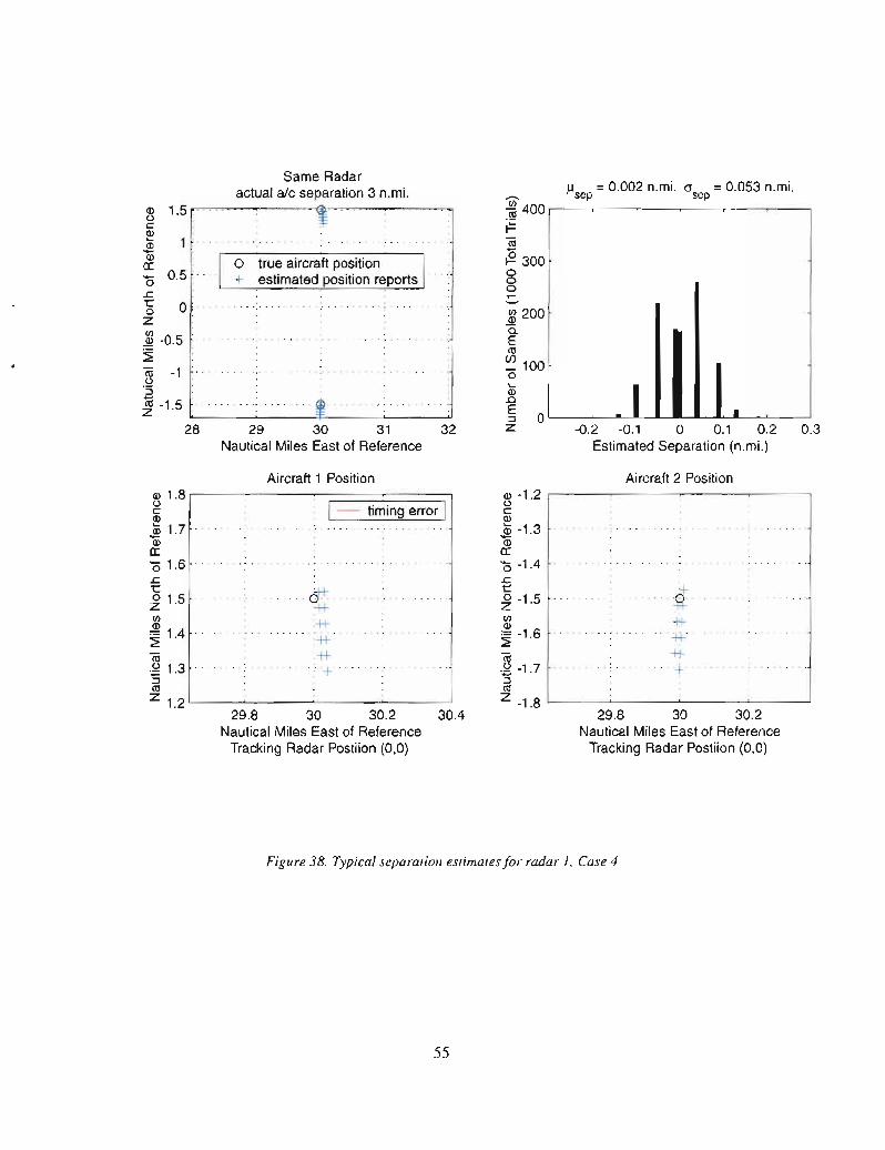
Same Radaractual alc separation 3 n.mi.
0.3-0.2 -0.1 0 0.1 0.2Estimated Separation (n.mi.)
81 200a.Eell
~ 100o
CD I~ 0 L-_---'- - ----l1h...J1 ---'__--.J
Z
f..l =0.002 n.mi. (J =0.053 n.mi._ sep sep'* 400 r-----..---,------r------,---,-----,
~
~~ 300aaa....
32
o true aircraft position+ estimated position reports
29 30 31Nautical Miles East of Reference
~ 1.5,c~$ 1.,Q)
c::'0 0.5"£;<5 0zen~ -0.5~(ij -1<>'S~ -1.5
"----~-----'F---~----'-'
28
Ai rcraft 1 Position Aircraft 2 Position
cfr-t+-t+:+t':-t+
.. :+
:t
*+t--1+-t+
'+
~ 1.81------::---:---;::::====:::::::::====~ai ' I - timing error I~ 1.7c::'0 1.6.L:
~ 1.5enQ)
~1.4
(ij.g 1.3:::lellz 1.2 L-__~ ,----__~~__----l
Q) -1.2 .----~-------.----~------,
<>cQ)
CD -1.3-Q)
c::'0 -1.4£;<5 -1 5z .enQ)
~ -1.6
(ij.g -1.7:::lellz -1.8 L-__~ -'--__--'~_ _____l
29.8 30 30.2 30.4Nautical Miles East of Reference
Tracking Radar Postiion (0,0)
29.8 30 30.2Nautical Miles East of Reference
Tracking Radar Postiion (0,0)
Figure 38. Typical separation estimates for radar 1, Case 4
55

29.8 30 30.2Nautical Miles East of ReferenceTracking Radar Postiion (60,0)
-++..... -t+ .
-++
*+++:t
+
-+++t++H-
.. -(j-c.
+t+.. it.
Same Radaractual alc separation 3 n.mi.
~ 1.5.·c~j!1(1)a: 0 true aircraft position'0 0.5.· + estimated position reports~
t~ 0(/)(1)
~ -0.5
«i.~ -1 .::J
~z -1.5'
28 29 30 31 32Nautical Miles East of Reference
Aircraft 1 Position~ 1.81--~--~-;===========:::;l55 I - timing error I~ 1.7(1)
a:'0 1.6£~ 1.5(/)
~ 1 4~ .«i.~ 1.3::J~z 1.2'----~---~----'------'
Ilsep=0.002 n.mi. cr =0.054 n.mi.
~ 400sep
ro~«i
;§ 300000..--l3 200a.Ero~ 1000
I....(1).0E
0 •::Jz -0.2 -0.1 0 0.1 0.2 0.3
Estimated Separation (n.mi.)
Aircraft 2 Position(1) -1.2 r---~---~---~----,c..lC(1)
Qj -1.3Qja:'0 -1.4£o -1 5z .(/)(1)
~ -1.6
«i.~ -1.7::J~z -1.8 '---__~ ~__~_______J
29.8 30 30.2Nautical Miles East of ReferenceTracking Radar Postiion (60,0)
Figure 39. Typical separation estimates for radar 2, Case 4
56

Different Radarsactual alc separation 3 n.mi.
0.3-0.2 -0.1 0 0.1 0.2Estimated Separation (n.mi.)
~ 200C.EIII
~ 100oQ;
~ 0 L-o~I-L-.IL.JLWL----...JI'"--_-L-_-'--_--'Z
Ilsep =-0.105 n.mi. 0sep =0.053 n.mi.~ 400 r--~---r------r---,---~----,III
~
lii~ 300ooo,....-
32
o true aircraft position+ estimated position reports
29 30 31Nautical Miles East of Reference
~ 1.5cQ)
~a:'0 0.5-£o 0zCIl
~ -0.5~
~ -1·5Ciiz -1.5 '----~-------'lF---~-----'
•
Aircraft 1 Position Aircraft 2 Position
e-+t++++-.. * .+++
++--+i++H
......-0+.+t+
.. ft
~ 1.81-~-----;-----;:::====:::::::====:=:;l
a5 I - timing error I2 1.7Q)
a:'0 1.6~
t:~ 1.5CIl
~14~ .
Cii.2 1.3:::J
Ciiz 1.2 L..-_---'- ~ ~ ~_'
29.8 30 30.2 30.4Nautical Miles East of Reference
Tracking Radar Postiion (0,0)
Q) -1.2 r---~---~---~-----,t.lCQ)
Q; -1.3Qia:'0 -1.4-£~ -1.5CIlQ)
~ -1.6
Cii.2 -1.7:::JCiiz -1.8 L..-__~ ~ ~__--'
29.8 30 30.2Natical Miles East of ReferenceTracking Radar Postiion (60,0)
Figure 40. Typical separation estimates independent radars, Case 4
57

29 30 31 32Nautical Miles East of Reference
o true aircraft position+ estimated position reports
++. '-4+
-4+.. G-+H-
+t-........... +f- .
+
+...... ~.
+t-.................. -i+....
+t.+.
Different Radarsactual alc separation 3 n.mi.
~ 1.5cQ)...
'*a:'0 0.5~
t::o 0Zen~ -0.5~
~ -1'S
~ -1.5w----~----T---~--~-'
28
Aircraft 1 Position~ 1.8 r------:------:----;:::=:=:::::=:=:===:;la5 I - timing error I~ 1.7a:'0 1.6~
~ 1.5enQ)
~1.4
Cii.2 1.3:::J
caz 1.2~-~---~---~---~
29.8 30 30.2 30.4Nautical Miles East of ReferenceTracking Radar Postiion (60,0)
J..l =0.111 n.mi. (J =0.056 n.mi._ sep sep.!!2 400 ,--~--,....----r--~--~-----,ell
iE:Cii
~ 300ooo,....-~ 200a.Eell
~ 100o
i 0 ~_----'-__""""'---'.L...L.JI~__........, --,,I_--L.......JZ -0.2 -0.1 0 0.1 0.2 0.3
Estimated Separation (n.mi.)
Aircraft 2 PositionQ) -1.2 r----~---~---~---___,(,)CQ)
Cii -1.3Qia:'0 -1.4£~ -1.5en~ -1 6~ .Cii.2 -1.7:::Jcaz -1.8 '------'---------'-------'------'
29.8 30 30.2Nautical Miles East of Reference
Tracking Radar Postiion (0,0)
Figure 41. Typical separation estimates additional case of independent radars, Case 4
58

Radar and Aircraft Geometry35 ,----.----~--____,--____,---._--___._--___.---,__--_.__--__,____,
30
25Q)(.)c
• Q)....220Q)
a:-0.r;to 15Zen~
~
(ij 10(.)
5enZ
5
o
* radar positiono aircraft position
- motion of aircraft in one minute
... ·*radar1····
. ·*radar2··
ac1
---08---0 .. ac2
-5 l--__-'--__--'- L--__-L.__------' -'--__---"- -'--__--'- -'--'
-5 o 5 10 15 20 25Nautical Miles East of Reference
30 35 40
Figure 42. Radar and aircraft geometry for Case 5
59

29 29.5 30 30.5 31 31.5Nautical Miles East of Reference
. I 0 tru~ aircrdaft p~~ition \ ...+ estimate position reports
Same Radaractual alc separation 3 n.mi.
0.3-0.2 -0.1 0 0.1 0.2Estimated Separation (n.mi.)
l3 2000.Ectl
~ 100o
i 0 '--_---'-__-'--_-----.......1 1"----'--------'----'z
Il =0.025 n.mi. 0' =0.010 n.mi._ sep sep~ 400 r------r---,....-----r -..,.--~--__,ctl
~]j~ 300ooo,....--t
. . . . . . . . . . . . ~~
Q)uc~~Q)
a:'0 0.5
£
~ o=~.(/)
.Q1
~_ -0.5ctl.2:::J
iii -1z28.5
Aircraft 1 Position Aircraft 2 Position
++t'ft+t
.......... ++-0
+
0.2 .............. : ... +t..
-++.++
-++o .... : ......... : .. -te.
+
Q) 0.3 ,-~---~----,----~---,ucQ)
~a:'0 0.1.ctoZ(/)Q)
~ -0.1
(ij.g -0.2:::JctlZ
~ 0.31-:---:---~==:::=======:::;lc 1- timing error I~~ 0.2Q)
a:'0 0.1£...~ 0(/)Q)
~ -0.1
(ij.g -0.2:::JctlZ
28.2 28.4 28.6 28.8Nautical Miles East of Reference
Tracking Radar Postiion (0,0)
31.2 31.4 31.6 31.8Nautical Miles East of Reference
Tracking Radar Postiion (0,0)
Figure 43. Typical separation estimates for radar I, Case 5
60

. : : -++*
... I 0 true aircraft position I+ estimated position reports
0.3-0.2 -0.1 0 0.1 0.2Estimated Separation (n.mi.)
~ 200a.Etil
~ 100o
Q; J~ 0 '--_-'---".L....I --.. .'---'--_----'
Z
)l =0.005 n.mi. (J =0.055 n.mi._ sep sep.!!2 400 r---r--~~---.--------,----r----,til
~
~~ 300oooT""-
Q)(,)c~
.l!1Q)
a:<5 0.5 .... _-_. '.-
L:t::~ 0_en~
~ -0.5"
29 30 31Nautical Miles East of Reference
Same Radaractual alc separation 3 n.mi.
co(,)
~ -1z
•
Aircraft 1 Position Aircraft 2 Position
+$$±±+......... <+:to···
~ 0.31--:-------:-;::::====::::::::====~c I - timing error I~
.l!1 0.2Q)
a:'0 0.1L:-o 0ZenQ)
~ -0.1
co.52 -0.2:::J11iz
Q) 0.3 ,----~~------,---~------."(,)C~
.l!1 0.2Q)
a:'0 0.1£;o 0ZenQ)
~ -0.1
co.2 -0.2 .:::J
11iz
28.2 28.4 28.6Nautical Miles East of ReferenceTracking Radar Postiion (30,30)
31.2 31.4 31.6 31.8Nautical Miles East of ReferenceTracking Radar Postiion (30,30)
Figure 44. Typical separation estimates/or radar 2, Case 5
61
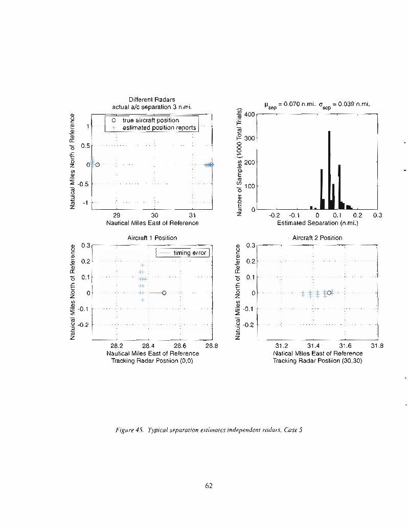
f..l. =0.070 n.mi. cr =0.039 n.mi._ sep sep"* 400 .---~--~-~--~-----.----,~
~~ 300ooo.....-
-0.2 -0.1 0 0.1 0.2Estimated Separation (n.mi.)
Q)uc~
Jl:1Q)
a:'0 0.5
£ozC/)
~
~ -0.5(iiu·SCii -1z
Different Radarsactual alc separation 3 n.mi.
I 0 true aircraft position I.. "1 + estimated position reports ..
........... -101#'
29 30 31Nautical Miles East of Reference
:ll200C.E(\l
~ 100oCo
~ 0 '--_---'-__-'------'..........1....z
_II.0.3
+.++ •........... +t+
++.++.-0.
+.
Aircraft 1 Position~ 0.31-~---~--;::====::::::=====~
c I- timing error I.~
Jl:1 0.2Q)
a:'0 0.1£o 0zC/)Q)
~ -0.1
(ii.2 -0.2:::JCiiZ
28.2 28.4 28.6 28.8Nautical Miles East of Reference
Tracking Radar Postiion (0,0)
. Aircraft 2 PositionQ) 0.3.----~---~---~---..."uC
~Jl:1 0.2Q)
a:'0 0.1£o 0zC/)Q)
~ -0.1
(ii.2 -0.2:::JCiiZ
31.2 31.4 31.6 31.8Natical Miles East of ReferenceTracking Radar Postiion (30,30)
Figure 45. Typical separation estimates independent radars, Case 5
62

28.5 29 29.5 30 30.5 31Nautical Miles East of Reference
o~""
0.3-0.2 -0.1 0 0.1 0.2Estimated Separation (n.mi.)
~ 200a.E(ll
~ 100
i 0 '-----_--'---'.1...L.-.1.......L...-l'"',·aJl.------'-------'----'
Z
Ilsep = -0.068 n.mi. (Jsep = 0.038 n.mi.~ 400 .-----r------,---,--~---,-------,(ll
~
~~ 300ooo.....---
31.5
Different Radarsactual alc separation 3 n.mi.
I0 true aircraft position I
"" + estimated position reports ""
QlUc!!!J!1Qla:'0 0.5£;...oZC/)
~
~ -0.5"iiiu'51ii -1z
Aircraft 1 Position Aircraft 2 Position
"+t
++" "-t+
++"+1+-1-'-------jO "
+:
~ 0.3 1 --:-------:--;::::==========:::;lc I - timing error I!!!J!1 0.2Qla:'0 0.1~
t~ 0C/)
Ql~ -0.1
"iii.2 -0.2 .:::J
1iiz
Ql 0.3r---~---"-----~---""uc!!!J!1 0.2Qla:'0 0.1£;...~ 0C/)
Ql~ -0.1
"iii.52 -0.2:::J
1iiz28.2 28.4 28.6
Nautical Miles East of ReferenceTracking Radar Postiion (30,30)
31.2 31.4 31.6 31.8Nautical Miles East of Reference
Tracking Radar Postiion (0,0)
Figure 46. Typical separation estimates additional case of independent radars, Case 5
63

5.3 SPECIFIC MEASUREMENTS
The purpose of developing a specific analysis capability is to be able to simulate the specific "hit"to "hit" performance that would be observed for specified radar locations and the specified flight paths oftwo aircraft. The individual measurements are recorded. The relative orientation and geometry of theaircraft to the radars will change for each measurement. The radar bias errors and aircraft transpondererrors are sampled once and held constant. The range and azimuth jitter errors vary "hit" to "hit." Theradar starting orientation is randomly selected and the update rate is randomly sampled between 4 and 5seconds and held constant for each radar. The specific times and true positions of the aircraft for each"hit" by each radar are calculated solving the simultaneous equations for the azimuth of the radar and thepositions of the aircraft, both continuous functions of time.
The case presented here involves two aircraft traveling towards radar 1 which might simulatearrivals at an airport near radar 1. The lead aircraft, aircraft 1, is traveling at a ground speed of 150 knotsand a heading of 217°. The second aircraft has a groundspeed of 185 knots and a heading of 224°. Theaircraft start out approximately 11 nautical miles apart and converge to approximately 3 nautical milesapart near radar 1. During the initial part of their paths the aircraft pass very near to radar 2. The runtimeis 12 minutes. The flight path and radar geometry is illustrated in Figure 47. A zoom in of a portion ofthe flight paths is shown in Figure 48 and illustrates the "hit" to "hit" variation. The blue dots are trackhits of the two aircraft by radar 1 and the red dots are track hits of the two aircraft by radar 2.
The results of this simulation are presented in Figures 49 through 54. Figures 49 and 50 plot theactual separation of the aircraft and the separation displayed on the radar screen as a function of time.Figure 50 is a zoom in of a portion of Figure 49 to show more clarity. The four sub-plots are the actualand displayed separation for the possible cases of each radar tracking each aircraft. The actual separationis a continuous function of time and is the same in all plots. The displayed separation is discontinuousand jumps as each aircraft's position estimate is updated on the screen. Note that even if there were zeroerror in the position estimates, the displayed separation estimate would be in error because the aircraftpositions were not estimated at the same time. For the case where radar 1 tracks both aircraft the error"spikes" seen are of short duration because the relative azimuth between the aircraft is small as seen fromradar 1. The flip-flop in the direction of the error spikes for the cases where radar 1 tracks both aircraftand radar 2 tracks both aircraft represents the point where the relative azimuths of the aircraft presented tothe radar change so that the first aircraft "hit" changes. The periodicity of the error spikes seen whendifferent radars are tracking the aircraft result from different update rates sampled for the radar. Thisresults in a periodic change in the relative timing of the radar "hits" on the two aircraft. This is similar tothe phenomena for example when observing windshield wipers on a bus driven by independent motors.Periodically they are in sync and out of sync.
Figures 51 through 53 plot the actual separation error (difference between the actual and displayedseparations presented above) as a function of time for two cases. The case where radar 1 tracks bothaircraft for the entire approach and the case where radar 2 tracks the aircraft until they are within 15nautical miles of radar 1 at which point radar 1 tracks the aircraft. In this second case there is a transition
64

period where radar 1 will be tracking aircraft 1 and radar 2 will be tracking aircraft 2 which can be seenupper plot of Figure 51. Figures 52 and 53 are zoomed in on portions of Figure 51 during the initialtracking period and during the transition period. This compares the performance of radar 1 tracking bothaircraft with the performance of radar 2 tracking the aircraft until they are within 15 nautical miles ofradar 1. Figure 54 are histograms of the separation errors in the initial tracking period and in thetransition period comparing the performance of having radar 1 track both aircraft with the performance ofhaving radar 2 track the aircraft initially and then transitioning to tracking by radar 1. They weregenerated by randomly sampling times during the initial period and transition periods and measuring theerror at those randomly sampled times. The small bumps in the histograms for radar 1 tracking bothaircraft that appear at approximately 2.5 nautical miles correspond to the spikes seen in Figures 52 and 53which are the display errors during the very short period between the updates of the two aircraft. A humanfactors study would be required to determine if these errors are significant and should be included.Similarly, the bifurcation in the histogram for the case of radar 2 tracking both aircraft is evident from the
error plots in Figure 52.
The conventional logic has been that in cases like this where a terminal radar is located at an airportand providing separation services for arriving (and departing) aircraft, and where the aircraft were farfrom the terminal radar (over 25 - 30 miles) but happen to be "passing by" a radar that was very near by(5-10 miles), performance would be enhanced by using the "radar of opportunity" while the aircraft werecloser to it. This would be accomplished through a mosaic display of that data to the terminal display.The rational is that radar positional accuracy degrades with distance from the radar so the separation
service would benefit from the greater accuracy of the nearby radar.
In the simulation presented here using the geometry described above the results show that this is notnecessarily the case for the following reasons.
First, while it is true that accuracy in general does degrade in range, range measurements in generaldo not, and in a geometry like this where aircraft are following in trail generally towards the airport, theseparation measurement is mostly a function of the difference in range measurements.
Second, aircraft in this geometry being tracked by the airport's radar generally have small azimuth
differences and thus move little between the hits on the two aircraft. But when tracked by the nearbyradar, the geometry is such that the azimuth is larger and thus the time between hits on the aircraft islarger. At typical speeds, this motion of the aircraft between hits can be the dominant error between theseparation displayed on the screen and the actual separation.
Third, there will necessarily be a period of transition when the aircraft nearest the airport is beingtacked by the airport's radar and the other aircraft by the "radar of opportunity." During this period thepositional errors are uncorrelated as are the update times so the errors in separation display are greatest.
65

30 •
25 .
QloCQl...~ 20·Qla: .'0£o 15 •z •(/)Ql
~cti 10 .o
+=:::JellZ
5
o.
* radar 1 location* radar 2 locationaircraft positions for radar 1 hitsaircraft positions for radar 2 hits
'irradar1 ;
4035305 10 15 20 25Nautical Miles East of Reference
o-5
-5 LL.-__---'- -'--__----' --'- L...-__---'- -'--__----'- -'--__--"
-10
Figure 47. Radar and aircraft tracking geometry for a specific case
66

21 ,-------,------,----:-0-----,----------,
20 .*radar 2' ..
""
".
Q)uc:~~Q)
II: 19'0-£...oZ(J)
~
~(ij 18u
+=':::J<0Z
i:I radar 1 locationi:I radar 2 location
aircraft position estimates for radar 1aircraft position estimates for radar 2
'.
17
1916 17 18Nautical Miles East of Reference
1516 L- --'-- -'- ----'- L- --'
14
Figure 48. Radar and aircraft tracking geometry for a specific case, zoom-in
67

11
-:- 10'E5 9c0 8:;::;ca~
ca 7Q.Q)
C/) 6()
~ 5
4
0
Radar 1 tracking Aircraft 1Radar 1 tracking Aircraft 2
.-'.-'.. true separation............ -.. -... est.. separation..
200 400 600time (sec)
Radar 1 tracking Aircraft 1Radar 2 tracking Aircraft 2
11
-:- 10"E5 9c0 8'';:::;
~ca 7Q.Q)
C/) 6()
~ 5
4
0
Radar 2 tracking Aircraft 1Radar 2 tracking Aircraft 2
200 400 600time (sec)
Radar 1 tracking Aircraft 2Radar 2 tracking Aircraft 1
11 11
-:- 10 ::: 10'E E5 9 5 9c c0 8 0 8~ ~~ ~
ca 7 ca 7Q. Q.Q) Q)
C/) 6 C/) 6() ()
~ 5 ~ 5
4 4
0 200 400 600 0 200 400 600time (sec) time (sec)
Figure 49. Displayed and actual separation as a function oftime for a specific case for each combination of radartracking aircraft
68

Radar 1 tracking Aircraft 1Radar 1 tracking Aircraft 2
8r---~---r--------,---,---~-----,
- truesepar~tion
- est. separation
co~ 7Cllc-al
(f)
~ 6.5
6'-----~-~---'----'--~----.J
330 340 350 360 370 380 390time (sec)
Radar 1 tracking Aircraft 1Radar 2 tracking Aircraft 2
-'g 7.5.scoeCllcal
(f)
~ 6.5
6 L.-_~_~__~_~__,_______.J
330 340 350 360 370 380 390time (sec)
Radar 2 tracking Aircraft 1Radar 2 tracking Aircraft 2
-'g 7.5.sco.~ 7Cllcal
(f)
~ 6.5
6L.-_~_~__~_~__,_______.J
330 340 350 360 370 380 390time (sec)
Radar 1 tracking Aircraft 2Radar 2 tracking Aircraft 1
8r-----r----r--------,---,---~-__,
-'g 7.5.sco.~
Cllcal
(f)
~ 6.5
6L.-_~_~__~_~__'_______.J
330 340 350 360 370 380 390time (sec)
Figure 50. Displayed and actual separation as a function oftime for a specific case for each combination of radartracking aircraft, zoom-in ofone minute during the middle of the track
69

Displayed Separation Error0.4 ,..---------r-----,-----,-----,----------r------.------r--l
Transition area
0.2
-0.2 .Radar2 tracks both aircraft Radar 1 tracks both aircra
700600500300 400seconds
200100
-0.4 L..- ----' ---l. --'- --'- --'-- ----'- --'---'
o
0.4 ,-------.,--I----'I--------r-----,,-------.,--I----'I-------,----,
0.2 ...:.-
-0.2 f- . ... ' Radar f tracks l)othalrcrafttheentireapproach· .
-0.4 <-- .<.-1 -'-1 ----'1 <--1 .<.-1 -1.1 ----'1----'
o 100 200 300 400 500 600 700seconds
Figure 51. Displayed separation error as afunction of time for specific case for radar 1 tracking both aircraftcompared with radar 2 tracking until aircraft are within 15 nmi range of radar 1.
70

Displayed Separation Error0.4 ,--------.------,-----,--------.------,--------,
0.2 f- . -
o
-0.2Radar 2 tracks both aircraft .
. -
320-0.4 '-- --' --'- .-J1'-- --"- '--1 ---'
200 220 240 260 280 300seconds
0.4 ,..--------,---------r------,------,...------,---------,
0.2
-0.2 .Radar 1 tracks both aircraft·
320300280260seconds
240220-0.4 '--------'--------'--------'-------'-------'---------'
200
Figure 52. Displayed separation error as a function oftime for specific case for radar J tracking both aircraftcompared with radar 2 tracking until aircraft are within J5 nmi range of radar J - two minutes of initial tracking.
71

Displayed Separation Error0.4 r--------.-----------r-----,..--------,------.---------,
0.2 ~
./
o
-0.2
Transition area-
-
540520500480seconds
-0.4 '----------'--------'1--------'----------'-------------'-------'
420 440 460
0.4 r-------,------,-----,..--------,------.---------,
0.2
-0.2 Radar 1 tr.acks both aircraft
540520500480seconds
460440-0.4 '---------'------------'-----....1..---------'-------'-----------'
420
Figure 53. Displayed separation error as a function oftime for specific case for radar J tracking both aircraftcompared with radar 2 tracking until aircraft are within J5 nmi range of radar J - transition area
72

Initial Tracking AreaRadar 1 tracking both aircraft
Initial Tracking AreaRadar 2 tracking both aircraft
-0.2 -0.1 0 0.1 0.2Nautical miles
Transition AreaRadar 1 tracking both aircraft
300
250C/)
a>
~ 200C'll
(f)
'0 150Q>.c 100E:::JZ
50
0
· = 0.034 •J.l.se~····· ....
.. :0 .. =.0.032· sep
300
250C/)
a>a.
200EC'll
(f)- 1500
Q>.cE 100:::JZ
50
0
Jlsep :;:: 0.034
.. :a .. =0.074. sep
-0.2 -0.1 0 0.1 0.2Nautical miles
Transition AreaDifferent radars tracking aircraft
300.---~-~--~-~--~--,
O'------~--~--
0.2-0.2 -0.1 0 0.1Nautical miles
300
250 l1sep= 0.019
C/)
a>= b.089a. 200 a
E• ·sep·······
C'll(f)- 1500....a>.c 100E:::JZ
50
00.2
l1sep = 0,039· .
a = 0.033.sep·
-0.2 -0.1 0 0.1
Nautical miles
250C/)
a>a. 200EC'll
(f) 150'0Q>.c 100E:::J
Z 50
Figure 54. Histograms ofdisplayed separation error in the initial tracking area and in the transition area for thecases where radar 1 tracked both aircraft and the cases where radar 2 tracked both aircraft in the initial tracking
area and radar 1 tracked the aircraft within a 15 nmi range.
73

6. SUMMARY AND CONCLUSIONS
An appropriate metric for measuring the performance of radars in providing separation services isthe error in separation presented to the controller. This is not easily deduced directly from the reportedpositional accuracy of the radar because the error sources have different characteristics. Some errors arecorrelated and will effect the positional estimates of two aircraft such that the error in separation isreduced. Some errors are direct functions of range and some are not. In addition, because the positionestimates are taken at different times, the separation displayed to the controller will have errors due to therelative motion of the aircraft between position estimates.
The approach taken in this analysis is to examine average separation errors, typical separationerrors, and specific separation errors, through Monte Carlo simulation based on the known errors inMode S surveillance. This simulation accounted for both correlated and non-correlated errors, includingthe important effect of the error introduced when aircraft positions are measured at different times bydifferent radars and presented to a controller on a mosaic display. These errors have not been included inprevious analysis (e,g, Ref. [1]).
The analysis for average separation errors show that the performance of radars in providingseparation services degrades with range. The analysis also shows that when using independent radars in amosaic display, errors in estimated separation will increase, on average, compared to the performancewhen providing separation with one radar. This is primarily because the bias errors and errors due tointer-sensor timing of position estimates are uncorrelated when using independent radars to estimate theseparation between two aircraft. The data presented in the section on average separation errors can besummarized by plotting the standard deviation of the separation error as a function of range for the singleradar case and for the independent mosaic display case. This is the standard deviation in averagemeasured separation error for two aircraft in trail three nautical miles apart in a random geometry. Thissummary is presented in Figure 55. Note that the mean of the estimated separations was three milesbecause all of the errors were sampled for each trial and the bias errors were averaged out in the results.
From Figure 55, it can be seen that the standard deviation of the error in displayed separation for asingle radar at a range of 40 nautical miles is 0.053 nautical mile. The standard deviation is 0.077nautical mile at the maximum typical range of a terminal radar (60 nmi.). This small difference indisplayed separation range (0.024 nmi. or 150 feet) is on the order of a wingspan of a transport aircraftand is in stark contrast to the large change in allowed separation standard (3 nmi. vs. 5 nmi. for aircraft atFU80 and below) for the two cases.
From Figure 55, the standard deviation of the separation measurement errors for independent radarswith a mosaic display is larger than that for a single radar, approximately three times as great in the 20 to40 nautical mile range. The increase in the standard deviation of the separation measurement errors atclose range is because the separation of the aircraft, three miles, causes an increase in the relative angle
75
between the aircraft on average and thus increases the delta time between hits which results in a greaterseparation error. This error begins to dominate at very short ranges.
It is also apparent that there is no range for independent radars with mosaic display that wi1l giveequivalent displayed separation performance, on average, as that of a single radar at 40 nautical miles.Therefore, it does not appear possible to argue that the single sensor separation standards should apply tomosaic display, purely on a surveillance equivalence basis. However, the relatively low values of thestandard deviation of displayed separation error (- 0.15 - 0.20 nmi.) for mosaic displays at ranges of 40to 60 nautical miles suggest that further safety analysis be performed to assess the application of 3 nmi.standards for terminal and mosaic displays.
The sections on typical and specific errors in separation measurements illustrate that the separationmeasurement errors are highly dependent on the geometry of the aircraft and radars. Applying averageresults to specific geometries can lead to counter intuitive results as was illustrated in the case presentedin the specific analysis.
76

0.251----,------r----~----!__;:=======:::::J========::;_
Single Mode S beaconMozaic Mode S beacon
'E.s 0.2...e...OJCo~Cllg- 0.15CIl
"0~::JCIlCllOJE
~ 0.1o~.~
"0
"ECll"0
~ 0.05C;;
.-.
. Actual Separation 3nmi .. .
:/". ,
.,/
,/.
. ,/
/'
605020 30 40range from radar to midpoint of two aircraft (nmi.)
10
OL-- ---'- --'---- -----JL- -L -L.- ----'
o
Figure 55. Standard deviation in measured separation error as a function of range for a single radar and forindependent radars with a mosaic display. Range is the distance from the radar(s) to a point midway between two
aircraft separated by 3 nautical miles as illustrated in Figure 4.
77

7. REFERENCES
l. Mosaic Display Target Accuracy Study, Final Report, for the Federal Aviation Administration,Under Contract DTFAOI-97-C-00046, ARCON Corporation, Waltham MA., December 13,1999.
2. J.L. Gertz, A.D. Kaminsky, COTS Fusion Tracker Evaluation, Project Report ATC-302,prepared for the Federal Aviation Administration, MIT Lincoln Laboratory, February 15,2002.
79

A. APPENDIX, MATLAB SIMULATION PROCEDURES AND SCRIPTS
The following sections describe the exact procedures used in creating the simulations described inthe body of the report. Each type of simulation is described with a step by step psuedo code descriptionfollowed by the MATLAB script that was used. The step numbers in the psuedo code descriptions matchthe step numbers in the scripts.
A.I AVERAGE ERRORS IN SEPARATION MEASUREMENTS, ONE RADAR
A.I.I Input
The range and samplesize are input to the simulation.
The range is the range of the aircraft from the radar in nautical miles. The two aircraft are assumedto be separated by three nautical miles and the range is to the point midway between the two aircraft.The aircraft will be randomly oriented about a circle whose origin is at the specified range. Thesamplesize is the number of cases that will be run.
A.I.2 Output
The outputs are vectors of length samplesize containing the separation estimates ES and positionerrors of the aircraft PEl and PE2. A histogram of the samples with the mean and standard deviation isplotted.
A.I.3 Modeling Procedure
I. Place the true radar position at the center of the coordinate system.
( xradartrue , yradartrue ) = ( 0 , 0 )
2. Define Common Digitizer format vectors that will be used to round off estimates to the nearestlI64 nautical mile in range and nearest lI4096 scan in azimuth (radians).
CDrange =[0 : lI64 : 100]
CDazimuth =[0 : 21rJ4096 :21t]
3. Define vectors of length samplesize of the true positions of the two aircraft. The two aircrafttrue positions are randomly oriented for each sample measurement with 3.0 miles separationsuch that the midpoint of the separation is at (range, 0). The first aircraft will be positioned at
81

( XaCtrue(acl) , yaCtrue(ac1) ) =( range + 1.5 * cos(q» , 1.5 * sin(q»)
and the second aircraft at
(xactrue(ac2j, yaCtrue(ac2» =(range - 1.5 * cos(q», -1.5 * sin(q»)
where q> is a vector of randomly selected angles between 0 and 360 degrees.
4. Compute vectors of the true range and azimuth from the radar for each aircraft. The azimuth is
computed in radians positive for positive yactrue(aci) and negative for negative yaCtrue(aci)
2 2rangetrue(aci) = sqrt (xac true(aci) + yac true(aci)
etrue(aci) =arctan ( yac true(aci) / xac true(aci) )
5. Define a vector of location bias errors by random sampling <\I from a uniformly distributedazimuth error between [0°, 360°] and locationbias from a uniformly distributed distance error of[0, 200] feet. Note that because this is an average computation the location bias error isresampled for each element in the vector. Determine the surveyed error in radar location.
( xradarsurveyerror, yradarsurveyerror) = ( locationbias* cos(<\I) , locationbias* sin(<\I»
6. Define a vector of range bias errors rangebias by random sampling from a uniform distributionbetween [-30, +30] feet. Note that because this is an average computation the range bias isresampled for each element in the vector. Note also that the same vector rangebias is used forboth aircraft.
7. Define two vectors of range jitter errors, one for each aircraft, rangejitter(acl) and rangejitter(ac2) byrandom sampling from a normal distribution with J..l =0 feet and () =25 feet.
8. Define two vectors of transponder range bias errors xponderbias(ac1) and xponderbias(ac2) byrandom sampling from a uniform distribution between [-125, + 125] feet. Note that because thisis an average computation the transponder range bias is resampled for each element of thevector.
9. Compute the estimated range for each aircraft as the true range plus the sum of the range errorsby adding the vectors
rangeestimate(aci) =rangetrue(aci) + ( rangebias + rangejitter(aci) + xpOnderbias(aci) ) / ( 6076.115 )
10. Compute a vector of the reported ranges for each aircraft as the estimated ranges rounded off tothe nearest 1/64 n. mi. This is done by linearly interpolating each of the value of rangeestimate(aci)
using the CDrange vector as both the x and y value for the function being interpolated and usingthe nearest neighbor option for the interpolation.
82

rangereportedlaci) = interp1(CDrange, CDrange , rangeestimatelaci), ,nearest')
11. Define a vector of azimuth bias errors 9bias by random sampling from a uniform distributionbetween [ _0.3 0
, +0.30]. Note that because this is an average computation the azimuth bias is
resampled for each element of the vector. Note also that the same vector 9bias is used for bothaircraft.
12. Define two vectors of azimuth errors, one for each aircraft, gerrorlac1) and gerrorlac2) by randomsampling from a normal distribution with M- =00 and 0" =0.0680
•
13. Compute the estimated azimuth for each aircraft as the true azimuth plus the sum of theazimuth bias and azimuth error by adding the vectors.
9estimate(aci) =9truelacil + ( 9bias + 9jitterlaci) )
14. Compute a vector of the reported azimuths for each aircraft as the estimated azimuths roundedoff to the nearest 114096 of a scan. This is done by linearly interpolating each of the values of9estimatelaci) using the CDazimuth vector as both the x and y value of the function being interpolatedand using the nearest neighbor option for the interpolation.
9reported(aci) =interp 1(CDazimuth, CDazimuth, gestimatelaci), ,nearest')
15. Compute vectors of reported aircraft x and y positions. This is based on the reported range andazimuth offset by the location bias.
xaCreportedlaci) =rangereported(aci)*Cos(9reported(aci) + xradarsurveyerror
yacreported(aci) =rangereported(aci,*sin(9reported(aci) + yradarsurveyerror
16. Compute vectors of errors in the reported aircraft x and y positions.
dxaC(aCi) =xacreported(aci) - xactrue(aci)
dyaclaci) =yacreportedlaci) - yactrue(aci)
PEi =sqrt ( dxac2(aci) + dyac2(aci) )
17. Define a vector of length samplesize of radar rotation rates radarrotationrate by random samplingfrom a uniform distribution between [21t15.0 , 21t14.0] radians per second. Note that becausethis is an average computation the rotation rate is resampled for each element in the vector.
18. Compute the error from timing errorclockbias on the separation measurements by dividing thedifference in azimuth between the two aircraft by the radar rotation rate to determine the timebetween "hits" and then multiplying the result by the assumed velocity of 200 knots. Aircraft I
83

is assumed to be the lead aircraft and aircraft 2 the trail aircraft. According to Figure 4, if thelead aircraft (aircraft 1) is "hit" first, then there is an apparent reduction in measured separation
and errorclockbias should be subtracted from the measured separation. If the trail aircraft (aircraft2) is "hit" first, then errorclockbias should be added to the measured separation. 9true(aci) is
computed as the arctan of ( yac true(aci) / xac lrue(aci) ) so a positive yac true(aci) results in a positivevalue for 9Irue(aci) and a negative yac true(aci) results in a negative value for 9true(aci). Recall in thismodel xac true(aci) is always positive. Therefore, if aircraft 1 has a positive value for yac true(acl)
and is therefore "hit" first, then the error should be subtracted. If aircraft 2 has a positive valuefor yac true(acll and is therefore "hit" first the error should be added. If we compute the clock biaserror in nautical miles according to the equation below, the error will be positive in value when
aircraft 1 is "hit" first and negative in value if aircraft 2 is "hit" first ( because 9true(acl) - 9true(ac2)
will be negative in value) and thus the value should always be subtracted from the estimatedseparation.
errorc10ckbias =( ( 9true(acl) - 9true(ac2) ) / radarrotationrate ) * ( 200/ 3600 )
19. Compute the vector of estimated separation from the reported position reports and the error dueto timing.
ES =sqrt ( (xacreported(acl) - xacreported(aC2i+ (yacreported(acl) - yacreported(ac21)2) - errorclockbias
20. Compute statistics on measurement errors. Compute the mean ~ and standard deviations cr ofthe values in the vectors PEl, PE2 and ES.
Plot the results. Plot histograms of the values in the vectors PEl, PE2 and ES for the rangemodeled and label the plots with the range and values of ~ and cr.
84

A.2 AVERAGE ERRORS IN SEPARATION MEASUREMENTS, TWO RADARS
A.2.1 Input
The range, samplesize, and E> are input to the simulation.
The range is the range of the aircraft from either radar in nautical miles. The relative angle E> is theangle from a line connecting the two radars to the center of separation of the two aircraft as illustrated inFigure 5. The distance between the two radars is adjusted to maintain the specified range. The twoaircraft are assumed to be separated by three nautical miles and the range is to the point midway betweenthe two aircraft. The aircraft will be randomly oriented about a circle whose origin is at the specifiedrange. The samplesize is the number of cases run.
A.2.2 Output
The outputs are vectors of length samplesize containing the separation estimates ES and positionerrors of the aircraft PEl and PE2. A histogram of the samples with the mean and standard deviation isplotted.
A.2.3 Modeling Procedure
1. Convert E> to radians and compute the true radar positions placing radar I at the center of thecoordinate system and the second radar so that they will both have a distance range to thecenter of the separation of the aircraft at an angle E> from the line connecting the radars.
E> = E> * (niI80)
( xradartrue(radarl), yradartrue(radarl) ) =(0 , 0 )
( xradartrue(radar2), yradartrue(radar2) ) =(2 * range * cos(E» , 0 )
2. Define Common Digitizer format vectors that will be used to round off estimates to the nearest1/64 nautical mile in range and nearest 1/4096 scan in azimuth (radians). Note that the possiblevalues of CDazimuth had to be extended from the one radar case. This is because the secondradar will see aircraft at the azimuth limits when E> =0 and additional errors introduced couldput the reported values over the conventional ± 1t limits.
CDrange = [-10164 : 1/64 : 100]
CDazimuth =[-5ni4: 2ni4096 :5ni4]
85

3. Define vectors of length samplesize of the true positions of the two aircraft. The two aircraft
true positions are randomly oriented for each sample measurement with 3.0 miles separation
such that the midpoint of the separation is at ( range*cos(8) , range*sin(8) ). The first aircraft
will be positioned at
(xaCtrue(acl), yactrue(ac1») = (range*cos(8) + 1.5 * cos(q», range*sin(8) + 1.5 * sin(q»)
and the second aircraft at
(xaCtrue(ac2), yactrue(ac2)) = (range*cos(8) - 1.5 * cos(q» , range*sin(8) - 1.5 * sin(q>))
where q> is a vector of randomly selected angles between 0 and 360 degrees.
4. a. Compute the vector rtcase of length samplesize that stands for radar tracking case. rtcase
will contain a I if aircraft 1 is nearest radar 1 and (necessarily from the geometry chosen)
aircraft 2 is nearest radar 2. rtcase will contain a 0 if aircraft I is nearest radar 2 and aircraft 2
is nearest radar 1. rtcaseopp will contain the opposite values of 0 and 1. The following analysis
computes all combinations of the two radars tracking the two aircraft and these vectors are used
to produce final statistical results under the assumption that the nearest radar will be tracking
the respective aircraft.
rtcase = I when xaCtrue(ac1) <= xactrue(ac2)
rtcase = 0 when xactrue(ac1) > xactrue(ac2j
rtcaseopp = 0 when xaCtrue(ac1) <= xactrue(ac2)
rtcaseopp= I when xaCtrue(ac1) > xactrue(ac2)
b. Compute vectors of the true range and azimuth from each of the radars to each aircraft of the
aircraft. The azimuth is computed in radians positive for positive yactrue(aci) and negative for
negative yactrue(aci)
rangetrue(radarj,aci) = sqrt ( (xac true(aci) - xradartrue(radarj»)"+ (yac true(aci) - yradartrue(radarj»)")
9 true(radarj,aci) = arctan ( (yac true(aci) - yradartrue(radarj) )/ (xac true(aci) - xradartrueiradarj») )
5. Define vectors of location bias errors for each radar by random sampling cl> from a uniformly
distributed azimuth error between [00, 3600
] and locationbias from a uniformly distributed
distance error of [0 , 200] feet. Note that because this is an average computation the location
bias error is resampled for each element in the vector. Determine the surveyed error in radar
location.
86

( xradarsurveyerror(radarj), yradarsurveyerror(radarj») =(]OCationbias/ COS(<pj) , ]ocationbias/ sine<p))
6. Define vectors of range bias errors rangebias(radarj) by random sampling from a uniformdistribution between [-30 , +30] feet. Note that because this is an average computation therange bias is resampled for each element in the vector. Note also that the same vectorrangebias(radarj) for a given radar is used for range computation to both aircraft by that radar.
7. Define four vectors of range jitter errors, one for each radar tracking each aircraft,rangejitter(radarj,aci) by random sampling from a normal distribution with Jl = 0 feet and cr = 25feet.
8. Define two vectors of transponder range bias errors xponderbias(aci) by random sampling from auniform distribution between [-125 , +125] feet. Note that because this is an averagecomputation the transponder range bias is resampled for each element of the vector.
9. Compute the estimated range from each radar to each aircraft as the true range plus the sum ofthe range errors by adding the vectors
rangeestimate(radarj,aci) =rangetrue(radarj,aci) + ( rangebias(radarj) + rangejitter(radarj,aci) + xponderbias(aci) )
/ (6076.115)
10. Compute a vector of the reported ranges for each radar to each aircraft as the estimated rangesrounded off to the nearest 1164 n. mi. This is done by linearly interpolating each of the value ofrangeestimate(radarj,aci) using the CDrange vector as both the x and y value for the function beinginterpolated and using the nearest neighbor option for the interpolation.
rangereported(radarj,aci) =interp1(CDrange , CDrange , rangeestimate(radarj,aci) ,'nearest')
11. Define a vector of azimuth bias errors for each radar 9 bias(radarj) by random sampling from auniform distribution between [ _0.3°, +0.3°]. Note that because this is an average computationthe azimuth bias is resampled for each element of the vector. Note also that the same vector9 bias(radarj) is used for both aircraft for a given radar.
12. Define vectors of azimuth errors for each radar tracking each aircraft, gerror(radarj.aci) by randomsampling from a normal distribution with Jl =0° and cr =0.068°.
13. Compute the estimated azimuth for each radar tracking each aircraft as the true azimuth plus thesum of the azimuth bias and azimuth error by adding the vectors.
gestimate(radarj,aci) =9 true(radarj,aci) + ( 9 bias(radarj) + 9jitter(radarj,aci) )
14. Compute a vector of the reported azimuths for each radar tracking each aircraft as the estimatedazimuth values rounded off to the nearest 114096 of a scan. This is done by linearly
87

interpolating each of the values of gestimate(radarj,aci) using the CDazimuth vector as both the x and yvalue of the function being interpolated and using the nearest neighbor option for theinterpolation.
9reported(radarj.aCi) = interp 1(CDazimuth, CDazimuth, gestimate(radarj,aci) " nearest')
15. Compute four vectors of reported aircraft x and y positions, one for each radar tracking eachaircraft. This is based on the reported range and azimuth offset by the location bias.
xaCreported(radarj,aci) = rangereported(radarj,aci)*cos(9reported(radarj,aci») + xradarsurveyerror(radarj)
yacreported(radarj,aci) = rangereported(radarj,aci)*sin(9reported(radarj,aci») + yradarsurveyerror(radarj)
16. Compute four vectors of errors in the reported aircraft x and y positions.
dxaC(radarj,aci) =xacreported(radarj,aci) - xactrue(aci)
dyaC(radarj,aci) =yacreported(radarj,aci) - yactrue(aci)
positionerror(radarj,aci) =sqrt ( dxac2(radarj,aci) + dyac2(radarj,aci) )
17. Compute two vectors of aircraft position errors if the nearest radar is tracking the aircraft. Thisis accomplished by multiplying, the vectors of 0 and I that were defined earlier and definewhich of the two cases (radar 1 tracking aircraft 1 and radar 2 tracking aircraft 2, OR, radar 1tracking aircraft 2 and radar 2 tracking aircraft 1) is true for each sample by the computedposition errors
PEl = rtcace*positionerror(radarl,ac1) + rtcaseopp* positionerror(radar2,ac1)
PE2 = rtcace*positionerror(radar2,ac2) + rtcaseopp* positionerror(radarl,ac2)
18. Define a two vectors of length samplesize of radar update rates updaterateradarj by randomsampling from a uniform distribution between [4.0, 5.0] seconds. Note that because this is anaverage computation the rotation rate is resampled for each element in the vector.
19. Determine the vector of length samplesize of maximum radar rotation rates.
maxupdaterate = max [ updaterateradart , updaterateradar2 ]
Compute a vector of the clock bias error clockbias on the separation measurements byrandomly sampling from a uniform distribution between -0.5 and 0.5 and multiplying by themaximum update rate and then multiplying by an assumed aircraft speed of 200 knots. Thetimes of radar "hits" are uncorrelated and can differ by as much as half of the maximum update
88
rate. The effect on apparent separation is randomly increased or decreased by the distance anaircraft travels during that time.
c10ckbias =(200 / 3600 ) * maxupdaterate * random [-0.5 , 0.5]
20. Compute the vector of estimated separation from the reported position reports and the clockbias error by first computing vectors for the two cases ES1122 (estimated separation whenradar 1 tracks aircraft 1 and radar 2 tracks aircraft 2) and ES 1221 (estimated separation whenradar 1 tracks aircraft 2 and radar 2 tracks aircraft 1) and multiplying by the appropriate radartracking cases vectors of 0 and I.
ESI122 =sqrt ( (xacreported(radarl,ac1) - xacreported(radar2,ac2))2 + (yacreported(radarl,ac1)
yacreported(radar2,ac2l) + clockbias
ESI22I =sqrt ( (xacreported(radarl,ac2) - xacreported(radar2,ac1)i + (yacreported(radarl,ac2)
yacreported(radar2,ac1l) + c10ckbias
ES = rtcase * ES1122 + rtcaseopp * ESI22I
21. Compute statistics on measurement errors. Compute the mean Il and standard deviations cr ofthe values in the vectors PEI,PE2 and ES.
Plot the results. Plot histograms of the values in the vectors PEI,PE2 and ES for the rangemodeled and label the plots with the range and values of Il and cr.
89

A.3 TYPICAL ERRORS IN SEPARATION MEASUREMENT
A.3.1 Input
The x and y positions of the two radars and the two aircraft (nmi from (0,0) reference), the heading(degrees) and ground speed (knots) of the aircraft, and the sample size are input.
xradartrue(radarl) , yradartrue(radarl)
xradartrue(radar2) , yradartrue(radar2)
xaCtrue(acl), yactrue(acl), head(acl) , grdspeed(ac1)
xaCtrue(ac2) , yactrue(ac2) , head(ac2) , grdspeed(ac2)
samplesize
A.3.2 Output
The outputs are vectors of length samplesize containing the position measurements errors andseparation measurement errors of the aircraft as follows:
PEll position error of radar I tracking aircraft 1
PE12 position error of radar I tracking aircraft 2
PE21 position error of radar 2 tracking aircraft I
PE22 position error of radar 2 tracking aircraft 2
ESEll12 estimated separation with radar I tracking aircraft 1 and radar I tracking aircraft 2
ESE2122 estimated separation with radar 2 tracking aircraft 1 and radar 2 tracking aircraft 2
ESE1l22 estimated separation with radar 1 tracking aircraft 1 and radar 2 tracking aircraft 2
ESE1221 estimated separation with radar I tracking aircraft 2 and radar 2 tracking aircraft 1
A.3.3 Modeling Procedure
1. Define Common Digitizer format vectors that will be used to round off estimates to the nearest1164 nautical mile in range and nearest 114096 scan in azimuth (radians).
90

CDrange = [-10164 : 1/64 : 100]
CDazimuth = [-51t14 : 21t14096 :51t14]
2. Define the update rates of the radars, urrl and urr2, by sampling once for each radar from auniform distribution between 4.0 and 5.0 seconds. Define the maximum update rate mur as thelarger of the two values.
3. Compute the true range (nmi) and azimuth (± radians, trig. orientation) from each of the radars
to each aircraft of the aircraft. The azimuth is computed in radians positive for positive
yactrue(aci) and negative for negative yactrue(aci)
rangetrue(radarj,aci) =sqrt ( (xac true(aci) - xradartrue(radarjl+ (yac true(aci) - yradartrue(radarj)2)
otrue(radarj,aci) =arctan ( (yac true(aci) - yradartrue(radalj) )1 (xac true(aci) - xradartrue(radarj» )
4. Define a location bias error for each radar by random sampling <I> from a uniformly distributedazimuth error between [00
, 3600] and locationbias from a uniformly distributed distance error of
[0, 200] feet. Note that because this is a typical computation the location bias error is sampledonly once and remains fixed for each radar throughout the remainder of the simulation.Determine the surveyed error in radar location.
( xradarsurveyerror(radarj) , yradarsurveyerror(radarj» =(locationbias/ cos(<l>j) , locationbiasj* sine<l>j»
5. Define a range bias error for each radar rangebias(radarj) by random sampling from a uniformdistribution between [-30 , +30] feet. Note that because this is an typical computation the rangebias is sampled once for each radar and remains fixed.
6. Define four vectors of range jitter errors, one for each radar tracking each aircraft,
rangejitter(radarj,aci) by random sampling from a normal distribution with J.l =0 feet and a = 25feet.
7. Define the transponder range bias error for each aircraft xponderbias(aci) by random samplingfrom a uniform distribution between [-125 , +125] feet. Note that because this is typicalcomputation the transponder range bias is sampled only once and remains fixed.
8. Compute vectors for the estimated range from each radar to each aircraft as the true range plusthe sum of the range errors by adding the errors. Note that rangeestimate(radarj,aci) ,
rangetrue(radarj,aci) and rangejitter(radalj,aci) are vectors of length samplesize and rangebias(radarj) andxponderbias(aci) are scalars. The true range is already in nautical miles but the errors are in feet,so they are converted to nautical miles.
91

rangeestimate(radarj,aci) == rangetrue(radarj,aci) + ( rangebias(radarj) + rangejitter(radarj,aci) + xpOnderbias(aci) )/ ( 6076.115 )
9. Compute vectors of the reported ranges for each radar to each aircraft as the estimated rangesrounded off to the nearest 1164 n. mi. This is done by linearly interpolating each of the value ofrangeestimate(radarj,aci) using the CDrange vector as both the x and y value for the function beinginterpolated and using the nearest neighbor option for the interpolation.
rangereported(radarj,aci) == interp I(CDrange , CDrange , rangeestimate(radarj,aci) " nearest')
10. Define a scalar value of azimuth bias error for each radar 9bias(radarj) by random sampling from auniform distribution between [ -0.3 0
, +0.3 0]. Note that because this is a typical computation,
the azimuth bias is sampled once for each radar and remains fixed.
II. Define vectors of length samplesize of azimuth jitter errors for each radar tracking eachaircraft, 9jitter(radarj,aci) by random sampling from a normal distribution with f..l == 0° and (j ==
0.068°.
12. Compute four vectors of length samplesize for the estimated azimuth for each radar trackingeach aircraft as the true azimuth plus the sum of the azimuth bias and azimuth error. The trueazimuth and azimuth bias are scalars and the azimuth errors are vectors of length samplesize.
gestimate(radarj,aci) =9true(radarj,aci) + ( 9bias(radarj) + 9jitter(~adarj,aci) )
13. Compute vectors of the reported azimuths for each radar tracking each aircraft as the estimatedazimuth values rounded off to the nearest 114096 of a scan. This is done by linearlyinterpolating each of the values of gestimate(radarj,aci) using the CDazimuth vector as both the x and yvalue of the function being interpolated and using the nearest neighbor option for theinterpolation.
9reported(radarj,aci) =interp I(CDazimuth, CDazimuth, gestimate(radarj,aci) ,'nearest')
14. Compute four vectors of reported aircraft x and y positions, one for each radar tracking eachaircraft. This is based on the reported range and azimuth offset by the location bias.
xaCreported(radarj,aci) =rangereported(radarj,aci)*cos(9reported(radarj,aci» + xradarsurveyerror(radarj)
yacreported(radarj,aci) =rangereported(radarj,aci)*sin(9reported(radarj,acij) + yradarSurveyerror(radarj)
15. Compute four vectors of errors, PElt, PE12, PE21, PE22, in the reported aircraft x and ypositions. These vectors are returned by the function.
dxaC(radarj,aci) =xaCreported(radarj,aci) - xaCtrue(aci)
92

dyaC(radarj,aci) = yacreported(radarj,aci) - yaCtrue(aci)
PE(radarj,aci) =sqrt ( dxaC2(radarj,aci) + dyaC
2(radarj,aci) )
16. Compute the vectors of estimated separation (before adding the error for clock bias) from thereported position reports.
ESll12 =sqrt ( (xaCreported(radarl,ac1) - xaCreported(radarl,aC2»2 + (yacreported(radarl,ac1) 2
yacreported(radarl,ac2») )
ES2122 =sqrt ( (xaCreported(radar2,ac1) - xaCreported(radar2,ac2»)2 + (yacreported(radar2,ac1) 2
yacreported(radar2,ac2») )
ESl122 =sqrt ( (xaCreported(radarl,ac1) - xaCreported(radar2,ac2»)2 + (yacreported(radarl,ac1)
yaCreported(radar2,aC2»)2)
ES1221 =sqrt ( (xaCreported(radarl,aC2) - xaCreported(radar2,ac1»)2 + (yacreported(radarl,ac2) J
yacreported(radar2,acl»)-)
17. Compute the timing error for the four combinations of radar tracking aircraft. These will beadded to ESl112, ES2122, ES1122, and ES1221 to calculate the apparent separation. The firststep is to calculate which aircraft is "hit" "first" by the radar. Between two aircraft, the aircraftdesignated as hit first is the one that minimizes the time between the hits of the two aircraft.For the two cases where the same radar is tracking both aircraft it is the aircraft that is hit firstwhile the radar is rotating clockwise. The azimuth notation is trigonometric from -1t to +1t.For the two cases where different radars are tracking different aircraft, the radars are assumeduncorrelated and the aircraft that is hit first is assumed random and the maximum difference intime between hits will be a randomly sampled value for up to half the maximum update rate.The track monitoring variables, tm1122aci , tm1221aci , tm1112aci , tm2122aci , are set equal to 1if aircraft i is hit second and thus will be the aircraft that apparently moved since the firstaircraft was hit. It will be set equal to 0 if aircraft i is the first aircraft hit and will not be movedin the computation of apparent separation. Thus tm1122ac1 = 1 means that for radar 1 trackingaircraft I and radar 2 tracking aircraft 2, aircraft I was hit second and will be moved. tm1122ac2
will necessarily be set to O.
s = random[ 0 , 1 ]
if s :::; 0.5, tm1122ac1 =1 and tm1122ac2 =0
else tm1122ac1 =0 and tm1122ac2 = I
93
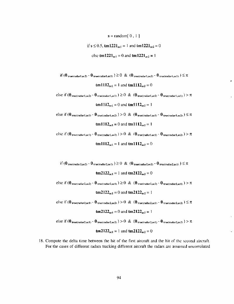
s =random[ 0 , 1 ]
if s ~ 0.5, tm1221acl = I and tm1221ae2 =0
else tm1221act =0 and tm1221ae2 = 1
if (8 true(radarl,ae2) - 8 true(radarl,ael) ) ~ 0 & (8 true(rad.rI,ae2l - 8 true(rad.rI,ael) ) ~ 1t
tml1l2ael =1and tmll12ae2 =0
else if (8 true(radarl,ae2) - 8 true(radarl,ael) ) ~ 0 & (8 true(r.darl,ae2) - 8 true(radarl,ael) ) > 1t
tml1l2ael =0 and tmll12ae2 =1
else if (8 true(radarl,ael) - 8 true(radarl,ae2) ) > 0 & (8 true(radarl,ael) - 8 true(radarl,ae2) ) ~ 1t
tml112ael =0 and tmll12ae2 = 1
else if (8 true(rad.rI,ael) - 8 true(radarl,ae2) ) > 0 & (8 true(radarl,ael) - 8 true(radarl,ae2) ) > 1t
tmll12ael = 1 and tmll12ae2 =0
if (8 true(rad.r2,ae2) - 8 true(r.d.r2,.el) ) ~ 0 & (8 true(rad.r2,ae2) - 8 true(radar2,ael) ) ~ 1t
tm2122ael = I and tm2122ae2 =0
else if (8 true(radar2,ae2) - 8 true(radar2,ael) ) ~ 0 & (8 true(radar2,ae2) - 8 true(radar2,ael) ) > 1t
tm2122ael =0 and tm2122ae2 = 1
else if (8 true(radar2,ael) - 8 true(radar2,ae2) ) > 0 & (8 true(radar2,ael) - 8 true(radar2,ae2) ) ~ 1t
tm2122ael =0 and tm2122ae2 = 1
else if (8 true(radar2,ael) - 8 true(rad.r2,.e2) ) > 0 & (8 true(radar2,ael) - 8 true(radar2,ae2) ) > 1t
tm2122ael =1 and tm2122ae2 =0
18. Compute the delta time between the hit of the first aircraft and the hit of the second aircraft.For the cases of different radars tracking different aircraft the radars are assumed uncorrelated
94

and the delta time is randomly chosen between zero and half the update rate of the slower radar.For the cases of the same radar tracking both aircraft the delta time is explicitly calculated.
cbdt1122 = (murl2)*random [ 0, I ]
cbdt1221 = (mur/2)*random [ 0 , I ]
if (9 true(radarl,acZ) - 9 true(radarl,ac1) ) :2:: 0 & (9 true(radarl,acZ) - 9 true(radarl,ac1) ) :::;; 1t
cbdt1112 = (urr1l21t)*(9 true(radarl,acZ) - 9 true(radarl,ac1»)
else if (9 true(radarl,ac2) - 9 true(radarl,ac1) ) :2:: 0 & (9 true(radarl,acZ) - 9 1rue(radarl,acl) ) > 1t
cbdt1112 = (urrl/21t)*[ 21t - (9 true(radarl,acZ) - 9 true(radarl,ac1»)]
else if (9 1rue(radarl,ac1) - 9 true(radarl,acZ) ) > 0 & (9 true(radarl,ac1) - 9 true(radarl,acZ) ) :::;; 1t
cbdt1112 = (urrl/21t)*(9 true(radarl,ac1) - 9 true(radarl,ac2) )
else if (9 1rue(radarl,ac1) - 9 true(radarl,acZ) ) > 0 & (9 true(radarl,ac1) - 9 true(radarl,acZ) ) > 1t
cbdt1112 = (urr1l21t)*[21t - (9 true(radarl,ac1) - 9 true(radarl,acZ»]
if (9 true(radarZ,acZ) - 9 true(radarZ,ac1) ) :2:: 0 & (9 true(radarZ,acZl - 9 true(radarZ,ac1) ) :::;; 1t
cbdt2122 = (urr2/21t)*(9 true(radarZ,acZ) - 9 true(radarZ,ac1) )
else if (9 true(radarZ,acZ) - 9 true(radarZ,ac1) ) :2:: 0 & (9 true(radarZ,acZ) - 9 true(radarZ,ac1) ) > 1t
cbdt2122 = (urr2/21t)*[21t - (9 true(radarZ,acZ) - 9 true(radarZ,ac1»]
else if (9 true(radarZ,ac1) - 9 1rue(radarZ,acZ) ) > 0 & (9 1rue(radarZ,ac1) - 9 true(radarZ,acZ) ) :::;; 1t
cbdt2122 = (urr2/21t)*(9 true(radarZ,ac1) - 9 true(radarZ,acZ»
else if (9 true(radarZ,ac1) - 9 true(radarZ,acZ) ) > 0 & (9 true(radarZ,ac1) - 9 true(radarZ,acZ) ) > 1t
cbdt2122 = (urr2/21t)*[21t - (9 true(radarZ,ac\) - 9 true(radarZ,ac2»)]
19. Compute the apparent x and y position for the aircraft that moved, i.e. the second aircraft hit.The tm variable which has a value of 1 for the aircraft hit second and a value of 0 for the
95

aircraft hit first is used to determine which aircraft is actually moved. This must be computedfor each combination of radar tracking each aircraft because the delta times and which aircraftis hit first depends on the which radars are tracking which airplanes. Note that heading is indegrees measured from north so delta x will be the sin of the heading and delta y the cos of theheading. The delta time is converted to hours because the ground speed is in knots. The xapparent is in nautical miles from the 0,0 reference point.
xac1112apparent(aciJ =xactrue(aci) + grdspeed(aciJ * sin«1tI180)head(aci) * cb~t1112/3600 *tmll12aci
xac2122apparent(aciJ =xactrue(aci) + grdspeed(aciJ * sin«1tI180)head(aci) ) * cb~t2122/3600 *tm2122aci
xac1122apparent(aci) =xactrue(aci) + grdspeed(aci) * sin«1tI180)head(aci) ) * cb~t1l22/3600 *tm1l22aci
xac1221apparent(aci) =xactrue(aci) + grdspeed(aci) * sin«1tI180)head(aci) ) * cb~t122113600 *tm1221aci
yac1112apparent(aci) =xactrue(aci) + grdspeed(aci) * cos«1tI180)head(aci) ) * cb~t1112/3600 *tm1l12aci
yac2122apparent(aci) =xaCtrue(aci) + grdspeed(aci) * cos«1tI180)head(aci) ) * cb~t2122/3600 *tm2122aci
yac1122apparent(aci) =xactrue(aci) + grdspeed(aci) * cos«1tI180)head(aci) ) * cb~t1122/3600 *tm1122aci
yac1221apparent(aci) =xactrue(aci) + grdspeed(aci) * cos«1tI180)head(aci) ) * cb~t122113600 *tm1221aci
20. Compute the true separation and the apparent separation. Note for the computation of apparentseparation the apparent x and y for both aircraft is used but the tracking monitor variable tmwill be 0 for one of the aircraft and so the apparent x,y will be the same as the true x,y.
7 7septrue = sqrt«xaCtrue(acl) - xactrue(ac2) t + (yaCtrue(acl) - yactrue(ac2) t)
sep1112apparent =sqrt«xac1112apparent(acl) - xac1l12apparent(ac2) )2 + (yac1112apparent(acl) yac1112apparent(ac2) )2)
sep2122apparent =sqrt«(xac2122apparent(acl) - xac2122apparent(ac2) )2 + (yac2122apparent(acl) yac2122apparent(ac2) )2)
96

sep1122apparent =sqrt«xac1l22apparent(acl) - xacI122apparent(ac2) )2 + (yac1l22apparent(acl)
yac1l22apparent(ac2) )2)
)
sep1221apparent =sqrt«xac1221apparent(acl) - xacI221apparent(ac2) t + (yac1221apparent(acl) -
yacI221apparent(ac2) )2)
21. Compute the clock bias as the difference between the apparent separation and the trueseparation.
cb1l12 = sep1l12apparent - Septrue
cb2122 = sep2122apparent - Septrue
cb1l22 =sep1l22apparent - Septrue
cb1221 = sep1221apparent - Septrue
22. Apply the clock bias to the separation calculated from the reported values of aircraft position.
ESI112 =ESI112 + cb1112
ES2122 = ES2122 + cb2122
ES1l22 = ES1122 + cb1122
ES1221 =ES1221 + cb1221
23. Compute the separation error for each combination of radar tracking aircraft
ESE1112 =ESI112 - Septrue
ESE2122 =ES2122 - Septrue
ESE1122 =ES1122 - septrue
ESE1221 =ES1221 - septrue
24. Compute the mean and standard deviations of the position errors and estimated separationmeasurement errors.
!lseparation errorl112 = mean[ESEII12]
!lseparation error2122 = mean[ESE2122]
!lseparation error1122 = mean[ESEI122]
97
O"separationerrorl112 = std[ESEl112]
O"separation error2122 = std[ESE2122]
O"separation error1l22 = std[ESEI122]

~eparation errorl221 =mean[ESEI221]
J.lpositionerror 11 = mean[PEll]
~ositionerror 12 = mean[PEI2]
~05itionerror 21 = mean[PE21]
~osition error 22 = mean[PE22]
O'separation errorl221 = std[ESE1221]
O'position error 11 = std[PEU]
O'position error 12 = std [PEI2]
O'positionerror21 = std [PE21]
O'position error 22 = std [PE22]
25. Before plotting, the reported aircraft posItIOns must be adjusted for clock bias. Thepresumption is that the positions input for the two aircraft are the true positions of the aircraft atthe time the first aircraft is hit. The plots of aircraft reported position must adjust the reportedpositions reports of the second aircraft hit to adjust for clock bias. The tm variable insures thatonly the reports for the second aircraft hit are moved.
xac1112reported(ad) =xaCreported(radarl,aci) + grdspeed(aci) * sin«7rl180)head(aci) * cbAt1112/3600 *tm1112aci
xac2122reported(aci) =xacreported(radar2,aci) + grdspeed(aci) * sin«7rl180)head(aci) ) * cbAt2122/3600 *tm2122aci
xac1122reported(acl) =xacreported(radarl,acl) + grdspeed(aclJ * sin«7rl180)head(acl» * cbAt1122/3600 *tm1122acI
xac1122reported(ac2) =xacreported(radar2,ac2) + grdspeed(ac2) * sin«7rl180)head(ac2» * cbAt1122/3600 *tm1122ac2
xac1221reported(acl) =xacreported(radar2,acl) + grdspeed(acl) * sin«7rl180)head(acl» * cbAt122113600 *tm1221acl
xac1221reported(ac2) =xacreported(radarl,ac2) + grdspeed(ac2) * sin«7rl180)head(ac2» * cbAt122113600 *tm1221ac2
yac1112reported(aci) =yacreported(radarl,aci) + grdspeed(aci) * cos«7rl180)head(aci» * cbAt1112/3600 *tml112ad
yac2122reported(aci) =yacreported(radar2,aci) + grdspeed(aci) * cos«7rl180)head(aci» * cbAt2122/3600 *tm2122aci
98

yac1122reported(acl) =yacreported(radarl,acl) + grdspeed(acl) *cos«1fI180)head(acl) ) * cbL1t1122/3600 *tm1122acl
yac1122reported(ac2) =yacreported(radar2,ac2) + grdspee~(ac2) * cos«1fI180)head(ac2») * cbL1t1122/3600 *tml122ac2
yac1221reported(acl) =yacreported(radar2,acl) + grdspeed(acl) * cos«1fI180)head(acl») * cbL1t122113600 *tm1221acl
yac1221reported(ac2) = yacreported(radarl,ac2) + grdspeed(ac2) * cos«1fI180)head(ac2) ) * cbL1t122113600 *tm1221ac2
26. Create four figures containing plots of the position estimates and true position of the aircraftand a histogram of the separation estimation errors, one for each combination of each radartracking each aircraft. Print out the mean and standard deviations of the errors on the graphs.
99

A.4 SPECIFIC ERRORS IN DISPLAYED SEPARATION
A.4.1 Input
The x and y positions of two radars and the initial positIOn of two aircraft (nmi from (Omreference), the heading (degrees) and ground speed (knots) of the aircraft, and the run time in seconds are
input.
xradartrue(radarl) , yradartrue(radarl)
xradartrue(radar2) , yradartrue(radar2)
xaCinitial(acl), yacinitial(acl), head(acl) , grdspeed(acl)
xaCinitial(ac2) , yacinitial(ac2) , head(ac2) , grdspeed(ac2)
runtime
A.4.2 Output
The outputs are vectors that containing a list of the position measurements errors and matrices ofthe displayed separation measurement errors as a function of time. The matrices of displayed separationmeasurement errors contain times in column I corresponding to an update by either radar and the
displayed separation error at that time. The displayed errors as a function of time will be linear betweenentries. The length of the vectors and matrices will depend on the individual radar rotation rates,
movement of the aircraft, and runtime. The output vectors and matrices are:
PEll position error of radar I tracking aircraft I
PE12 position error of radar I tracking aircraft 2
PE21 position error of radar 2 tracking aircraft I
PE22 position error of radar 2 tracking aircraft 2
ESE1112 displayed separation with radar I tracking aircraft I and radar I tracking aircraft 2 vs. t
ESE2122 displayed separation with radar 2 tracking aircraft I and radar 2 tracking aircraft 2 vs. t
ESE1l22 displayed separation with radar I tracking aircraft I and radar 2 tracking aircraft 2 vs. t
ESE1221 displayed separation with radar I tracking aircraft 2 and radar 2 tracking aircraft I vs. t
100

A.4.3 Modeling Procedure
I. Define Common Digitizer format vectors that will be used to round off estimates to the nearest1/64 nautical mile in range and nearest 1/4096 scan in azimuth (radians).
CDrange = [-10/64: 1164: 100]
CDazimuth = [-57f14 : 27f14096 :57f14]
2. Define the update rates of the radars, urr1 and urr2, by sampling once for each radar from auniform distribution between 4.0 and 5.0 seconds.
3. Define the radar start times tsrl and tsr2 by sampling once for each radar between 0 and theupdate rate of that radar.
4. Compute the samplesizes for the two radar hits as the number of rotations during the runtime.fix rounds down to the next lowest integer.
samplesizei =fix«runtime-tsri)/urri)
5. Compute vectors of the times of the hits of each radar i on each aircraft j thij. This is done byfinding the zeros of the function describing the difference between the time dependent angle ofthe radar and the time dependent equation describing the aircraft's angular relationship to theradar. The zeros of the function describing the difference in these angles is found withinspecified limits corresponding to each single rotation of the radar.
The aircraft x and y positions as a function of time are described by:
aCjx(t) =XaCinitial(a<jl + (grdspeed(acj) 13600) * t * sin(head(acj) * (1T/180))
aCjy(t) =yacinitial(acj) + (grdspeed(a<j) I 3600) * t * cos(head(acj) * (7fl180))
and the aircraft position angle relative to the radar as:
arctan «acjy(t)- yradartrue(radari) ) I (acjx(t)- xradartrue(radari) )
The angle of the radar is expressed as a discontinuous function of time t between -1t and +1t for eachrotation i of the radar starting with i = I:
1t - 21t ( (t - ( tsrradari+ (i - I ) * urrradari ) ) I urrradari )
101

The times of hit for radar i on aircraft j thij consists of finding the zeros of the difference of theangles, or solving, for each rotation k of the radar i, the equation:
[ It - 2It ( (t - ( tsrradari+ (k - I ) * urrradari ) ) / urrradari ) ] - [arctan «acjy(t)- yradartrue(radari) ) /(acjx(t)- xradartrue(radari) ) ] =0
6. Next compute the vectors of true x an y positions of the aircraft j when they are hit by radar i
xacijtrue =xacinitial(aq') + (grdspeed(ag") /3600) * thij * sin(head(acj) * (1tI180))
yacijtrue = yacinitial(acj) + (grdspeed(aq') /3600) * thij * cos(head(acj) * (1tI180))
7. The geometry of the radars and the true positions of the aircraft when hit by the radars isplotted.
8. The next step is to plot the apparent separation caused by the "clock bias" or fact that theaircraft are hit at different times and are moving between display updates. This is theseparation that appears on the radar screen as a function of time. This is done for each of thefour combinations of radar tracking aircraft (i.e. radar I tracking aircraft I and radar 2 trackingaircraft 2.)
8 a. First create combination vectors of the hit times. tcoml112 is a vector for all of the hit timesfor radar I hitting aircraft I and radar I hitting aircraft 2. This is created by concatenating andsorting thll and th12. Create tcomll12 tcom2122 tcom1l22 and tcom1221.
8 b. Eliminate any duplicate entries in tcomll12 tcom2122 tcom1l22 and tcom1221.
8 c. Replicate each time hit entry and shift the value of one entry th - £ and one entry th + £ andthrow out the first entry in the vector. These vectors, tcomrepll12, tcomrep2122,tcomrep1l22 and tcomrep1221 contain a sorted list of hit times of both aircraft except oneentry is just before the hit and one entry is just after the hit. This allows linear interpolationholding separation values constant between update times.
8 d. Similarly create replicated time vectors of the individual vectors thll, th12, th21, and th22that contain values of one entry th - £ and one entry th + £ and throw out the first entry in thevector. These vectors are called thllrep, th12rep, th21rep, and th22rep.
8 e. Create replicated vectors xaclltruerep, xac12truerep, xac2ltruerep, xac22truerep,yaclltruerep, yac12truerep, yac2ltruerep, yac22truerep for the true x and y positions ofthe aircraft when they are hit by each radar and eliminate the final entry.
8 f. Create matrices DISPll12, DISP2122, DISP1l22, DISP1221 of the displayed positions foreach combination of radar tracking aircraft, i.e. DISP1l22 is a matrix for the case of radar I
102
..

tracking aircraft 1 and radar 2 tracking aircraft 2. The first column contains the replicated times
for all hits, tcomrep for the respective tracking case, i.e. the first column of DISP1l22 contains
tcomrep1l22. The second, third, fourth, and fifth columns are the x and y values of aircraft 1
and 2 respectively at the times in column I. These are obtained by linearly interpolating the
replicated values of x and y versus the replicated times. For example, column 2 of DISP1l22contains the x values of aircraft 1 at the times in column 1, tcomrep1l22, obtained by linearlyinterpolating thllrep versus xaclltruerep for the times in tcomrep1l22. The sixth and
seventh columns contain the ~x and ~y values of the aircraft and the eight column contains thedisplayed separation (with no radar errors) as a function of the time in column 1. The
replication of times ±E allows for the displayed separation to be constant between updates as it
would be displayed on a radar screen.
8 g. Create a function for the true separation of the aircraft as a function of time based on their
initial positions, and constant headings and groundspeeds.
8 h. Plot the displayed target separation with no radar error, due only to clock bias, versus the true
separation as a function of time for all combinations of radar tracking aircraft. The differencebetween the displayed and true separation is due only to the movement of the aircraft between
radar hits.
9. Compute the true ranges and azimuths at the times of radar hit for all combinations of radars
tracking aircraft. rangeijtrue and 8ijtrue refer to range and azimuth for radar i hitting aircraft j at
the times radar i hit aircraft j.
rangetrue(radari,acj) = sqrt«(xacijtrue - xradartrue(radari»A2 + (yacijtrue - yradartrue(radari)A2)
E>true(radari,aCj) =arctan« yacijtrue - yradartrue(radari»/( xacijtrue - xradartrue(radari»)
1o. Define radar site location bias errors xradarsurveyerror(radari) , yradarsurveyerror(radari) by samplingonce for each radar from a uniform random direction [0-360°] and a uniform random distance[0-200]feet and convert to nautical miles.
11. Define a range bias error for each radar rangebias(radari) by a random sampling from a uniformdistribution between [-30, +30] feet once for each radar.
12. Define four vectors of range jitter errors, one for each radar tracking each aircraft,
rangejitter(radari,acj) by random sampling from a normal distribution with Il = 0 feet and cr = 25feet. Sample once for each radar hit thij. The lengths of the vectors will be different dependingon how many times a radar hit an aircraft.
13. Define the transponder range bias error for each aircraft xponderbias(alj) by random samplingonce for each aircraft from a uniform distribution between [-125 , + 125] feet.
103

14. Compute vectors for the estimated range from each radar to each aircraft for each hit as the truerange plus the sum of the range errors by adding the errors.
rangeestimated(radari,acj) = rangetrue(radari,acj) + ( rangebias(radari) + rangejitter(radari,acj) + xponderbias(acj) )/ ( 6076.115 )
15. Compute vectors of the reported ranges for each radar to each aircraft as the estimated rangesrounded off to the nearest 1/64 n. mi. This is done by linearly interpolating each of the value ofrangeestimated(radari,acj) using the CDrange vector as both the x and y value for the function beinginterpolated and using the nearest neighbor option for the interpolation.
rangereported(radari,acj) =interp 1(CDrange , CDrange , rangeestimated(radari,acj)' nearest')
16. Define a value for radar azimuth bias error for each radar 9bias(radari) by random sampling from auniform distribution between [ -0.3 0
, +0.3 0]. Note that because this is a typical computation,
the azimuth bias is sampled once for each radar and remains fixed.
17. Define vectors of the length of thij of azimuth jitter errors for each radar tracking each aircraft,9jitter(radari,acj) by random sampling from a normal distribution with IJ- = 00 and cr = 0.068 0
•
Convert to radians.
18. Compute four vectors of the length of thij for the estimated azimuth for each radar trackingeach aircraft as the true azimuth plus the sum of the azimuth bias and azimuth error. The trueazimuth and azimuth bias are scalars and the azimuth errors are vectors of the length of thij.
gestimate(radari,acj) =9true(radari,acj) + ( 9bias(radari) + 9jitter(radari,acj) )
19. Compute vectors of the reported azimuths for each radar tracking each aircraft as the estimatedazimuth values rounded off to the nearest 1/4096 of a scan. This is done by linearlyinterpolating each of the values of gestimate(radari,ag') using the CDazimuth vector as both the x and yvalue of the function being interpolated and using the nearest neighbor option for theinterpolation.
9reported(radari,acj) = interp I(CDazimuth , CDazimuth, gestimate(radari,ag') " nearest')
20. Compute the vectors of reported x y positions for both aircraft for both radars.
xacijreported =rangereported(radari,acj) * cos(9reported(radari,aCj») + xradarsurveyerror(radari)
yacijreported = rangereported(radari,ag') * sin(9reported(radari,acj») + yradarsurveyerror(radari)
21. Compute and return the vectors of distance errors in reported position of the aircraft.
/ixacij =xacijreported - xacijtrue
104

!::t.yac:ij =yacijreported - yacijtrue
PEij = sqrt(!::t.xacij "2 + !::t.yacij "2)
22. Plot the geometry of the radars and the displayed positions of the aircraft when hit by theradars.
23. Compute and plot the apparent or displayed separation versus time for position reports thatinclude the errors and the clock bias.
23 a. Create replicated vectors for the reported x and y position reports of the aircraft when theyare hit by each radar and eliminate the final entry. xacllreportedrep, xac12reportedrep,xac21reportedrep, xac22reportedrep, yacllreportedrep, yac12reportedrep,yac21reportedrep, yac22reportedrep.
23 b. Create matrices ADISPll12, ADISP2122, ADISP1l22, ADISP1221 of the displayedpositions for each combination of radar tracking aircraft, i.e. ADISP1l22 is a matrix for thecase of radar 1 tracking aircraft I and radar 2 tracking aircraft 2. The first column contains thereplicated times for all hits, tcomrep for the respective tracking case, i.e. the first column ofADISP1l22 contains tcomrep1l22. The second, third, fourth, and fifth columns are thereported values of x and y for aircraft 1 and 2 respectively at the times in column 1 which aredisplayed on the radar screen. These are obtained by linearly interpolating the replicated valuesof reported x and y created in step 23a. versus the replicated times. The replication of timesand position reports is necessary to hold the displayed values of x and y constant betweenupdates. For example, column 2 of ADISP1l22 contains the reported (displayed) x values ofaircraft I at the times in column 1, tcomrep1l22, obtained by linearly interpolating thllrepversus xacllreportedrep for the times in tcomrep1l22. The sixth and seventh columnscontain the L\x and L\y values of the aircraft and the eight column contains the displayedseparation including radar errors as a function of the time in column 1. The replication oftimes ±E allows for the displayed separation to be constant between updates as it would bedisplayed on a radar screen.
23 c. Plot the displayed (reported) target separation as a function of time versus the trueseparation for all combinations of radar tracking aircraft. The difference between the displayedand true separation is due to both position reporting errors and the movement of the aircraftbetween hits by the radar.
24. Create and return the matrices of errors in the separation measurements.
ESEl112 displayed separation with radar I tracking aircraft I and radar 1 tracking aircraft 2 vs. t
ESE2122 displayed separation with radar 2 tracking aircraft I and radar 2 tracking aircraft 2 vs. t
105

ESE1122 displayed separation with radar I tracking aircraft I and radar 2 tracking aircraft 2 vs. t
ESEI221 displayed separation with radar I tracking aircraft 2 and radar 2 tracking aircraft I vs. t
24 a. Use temporary matrices TESE for computations and return two columns in the form ofESE. The first column of TESEI112, TESE2122, TESE1122, and TESE1221 contain the firstcolumn of the respective ADISP matrix, the replicated times for all radar hits.
24 b. Compute the true values of x and y for aircraft I and 2 at the times in column I and placethem in columns 2 through 5 respectively of TESE1112, TESE2122, TESE1122, andTESE1221 using the aircraft initial positions, groundspeeds and headings.
24 c. Compute the delta x and delta y values of between the aircraft and put them in columns 6and 7 respectively of TESE1112, TESE2122, TESE1122, and TESEI221.
24 d. Compute the actual separation from the delta x and delta y values and place in columns 8 ofTESEI112, TESE2122, TESE1122, and TESEI221.
24 e. Copy the displayed separation from column 8 of ADSIPI112, ADSIP2122, ADSIP1122,ADSIPI221, into column 9 of TESE1112, TESE2122, TESE112, and TESEI221.
24 f. Compute the error between the displayed separation in column 9 and the actual separation incolumn 8 and place the separation error in column 10 of TESE1112, TESE2122, TESE112,and TESEI221.
24 g. Return the matrices of estimated separation errors versus time, ESE1112, ESE2122,ESE1122, and ESE1221 by copying the times from column I into column I and the errors indisplayed separation from column 10 into column 2 from TESEI112, TESE2122, TESE112,and TESE1221 respectively. The ESE matrices will contain the replicated times in column Iand the separation errors in column 2. The errors will jump with the discontinuity of the updateand will vary linearly between updates. For instance, if aircraft are maintaining a constantseparation then the error will be constant until the next update, but if the aircraft are changingseparation there will be a linear change in error as a faction of time until the next discontinuityat the next update.
106
..