analyses of experiments and a functional model for …
TRANSCRIPT

ANALYSES OF EXPERIMENTS AND A FUNCTIONAL MODEL
FOR SHIP ROLLING
A Thesis submitted for the degree of Doctor of Philosophy
by
J an Mathisen
Department of Mechanical Engineering, BruneI University
September 1988

0-2
Abstract
Simulation techniques and a Volterra functional polynomial are applied as two alter
native methods of calculating ship roll response to irregular waves. The roll motion is
modeled by a single degree of freedom differential equation, with two alternative nonlinear
damping functions. Estimation techniques are developed to obtain the coefficients of the
damping functions from decay tests and from forced rolling tests. A linear plus quadratic
form of damping function is found to be slightly preferable to a linear plus cubic form.
The roll response process is found to be non-Gaussian, and characterised by negative
values of the coefficient of kurtosis. Simulation results agree well with results obtained
from the functional polynomial for low response levels, but show increasing disagreement
as the response level increases, due to divergence of the functional polynomial representa
tion.
Analyses of results from model tests in irregular waves and from sea trials confirm
the non-Gaussian nature of the roll response. A "constrained" form of the generalised
gamma distribution function is found to provide an improved fit to the roll maxima and to
the roll minima, as compared to the Rayleigh distri~ution. The model tests also show
some asymmetry in the roll response, which is not predicted by the theoretical model. It is
suggested that this asymmetry may primarily be due to the combined effect of horizontal
drift forces and the restraining system used to keep the model on station.

Contents
Section
1.
1.1
1.2
1.3
1.4
1.5
1.6
1.7
2.
2.1
2.1.1
2.2
2.2.1
2.2.2
2.2.3
2.3
2.4
2.4.1
2.4.2
2.5
2.5.1
2.5.2
2.5.3
Abstract
Contents
Acknowledgements
Introduction
Historical Background
Linear Equations for Coupled Rolling
Advances on Strip Theory
Single Degree of Freedom, Linear Equation for Rolling
Nonlinearities Affecting Rolling
Rolling as a Stochastic Process
An Overview of the Present Investigation
Direct Time Simulation of Rolling
Reformulation of Equations of Motion
0-3
Procedure for Frequency-Dependent, Linear Added-Mass and Damping
Roll Excitation Function
Checking Simulation of Random Wave Elevation
Interpolation on Excitation Signal
Initial Tapering of Excitation Signal
Numerical Integration Technique
Simulation Parameters
Time Step
Tolerances
Some Simulation Results
Simulation of Roll Decay
Roll Response to Harmonic Excitation
Irregular Waves
Page
0-2
0-3
0-7
1-1
1-1
1-3
1-7
1-8
1-9
1-13
1-16
2-1
2-1
2-1
2-3
2-6
2-7
2-9
2-9
2-9
2-10
2-10
2-11
2-11
2-13
2-16
Section
3.
3.1
3.2
3.2.1
3.3
3.4
3.4.1
3.4.2
3.5
3.5.1
3.5.2
3.5.3
4.
4.1
4.2
5.
5.1
5.2
5.3
5.4
5.5
5.6
5.7
5.8
5.9
5.9.1
5.9.2
5.9.3
A Functional Model for Ship Rolling
Linear Systems Theory
A Functional Polynomial for Nonlinear Rolling
Numerical Evaluation of Roll Response Spectrum
The Edgeworth Probability Distribution
The Generalised Gamma Probability Distribution
A Constraint on the Generalised Gamma Distribution
Estimation of Parameters
Some Results with the Functional Model
Visualisation of the Cubic Transfer Function
Response to Harmonic Excitation
Response to Irregular Waves
Long Term Distribution of Roll Response
Basic Derivation of Long Term Distribution
Further Aspects of the Long Term Distribution
Time Series Analysis Program
The Database
cdf Cumulative Distribution Function Plot
coy Covariance Function
dcy Roll Decay Test Analysis
dec Decimation
dif Differentiation
eng Envelope Process on Energy Basis
env Envelope Process Using Hilbert Transform
fit Fit of Unidimensional Distribution Functions to Data
Normal Distribution
Edgeworth Distribution
Rayleigh Distribution
0--4
Page
3-1
3-1
3-4
3-7
3-9
3-13
3-13
3-15
3-16
3-16
3-21
3-23
4-1
4-1
4-3
5-1
5-2
5-6
5-7
5-7
5-7
5-8
5-10
5-10
5-13
)~13
5-14
5-14

0-5
Section Page
5.9.4 Constrained Generalised Gamma Distribution 5-14
5.9.5 x2 Test of Fit 5-14-
5.9.6 Testing Fit of Tails of Distribution Functions 5-16
5.10 flt Filter and Wild Point Editing 5-18
5.11 gen Generate Test Data 5-18
5.12 hrm Harmonic Analysis 5-19
5.13 lea Level Crossing Analysis 5-21
5.14 ppp PP-Plot 5-22
5.15 psd Power Spectral Density 5-22
5.16 stn Stationarity Check Along a Sample Record 5-24
5.17 tnd Detrending 5-27
6. Estimation of Roll Damping Coefficients 6-1
6.1 Estimation of Roll Damping Coefficients from Experiments 6-4
6.2 Results from Estimation of some Damping Coefficients 6-4
6.2.1 Damping Coefficients for the "FPV Sulisker" 6-5
6.2.2 Damping Coefficients for a Containership 6-8
6.3 Check of Estimators from Simulation Results 6-10
7. Results of Analysis of Experimental Data for Ship Rolling 7-1
in Irregular Waves
7.1 The Irregular Wave Tests 7-1
7.2 Visualisation of the Data 7-2
7.3 Stationarity Check 7-6
7.4 Detrending and Filtering 7-12
7.5 Wave and Roll Spectra 7-14
7.6 Distribution of Continuous Signals 7-19
7.7 Distributions of Maxima and Minima 7-26
7.8 Additional Results from Model Tests on an Elliptical Hull 7-34
7.9 Additional Results from Full Scale Tests with the CFA V QUEST 7-35

Section
7.10
8.
9.
10.
A
B
C
0-6
Correlation between Kurtosis and Slope Paramo of Gamma Distribution
Conclusions
References
Notation
Appendices
Bibliography
The Roll Exciting Moment
Derivations for Volterra Functional Polynomials
D Estimation of Ship Roll Damping Coefficients
Page
7-39
8-1
9-1
10-1
A-I
B-1
C-1

0-7
Acknowledgements
My wife, Anne Grethe Mathisen, has encouraged me, from emergence of the idea of
postgraduate studies, and throughout their course. She has carried a portion of my family
duties, and accepted the effects on our way of life. Our children, Karen Marie and Nils
Mikal, have endured the diversion of my attention with a fair degree of patience, while my
parents, Karen Erika and Birger Mathisen, have given of their time and attention to the
children, and offered me their encouragement.
When I first discussed the possibility of postgraduate studies with my boss in Veritas
at that time, Harald Olsen, his positive reaction was instrumental in encouraging me to
pursue the idea. Subsequent reorganisations provided me with several different superiors
at Veritas (Odd A. Olsen, Per Otto Araldsen, Henrik Madsen, Pal Bergan, Odd Tore Sau
gerud), who have all encouraged me and who have also provided more tangible assistance
to the pursuit of my studies.
Geraint Price answered my initial enquiry to University College London, about post
graduate studies, in a personal and direct way, which served to initiate a trusting relation
ship. This lead me to follow him to BruneI University when he took up his professoriate
there. As my supervisor, he has provided a balanced mixture of encouragement, ques
tions, guidance and patience, which has suited me very well.
The research group associated with Prof. Price (Job Baar, Fu Yuning, Toichi Fuka
zawa, Takeshi Kinoshita, Mikhail Leontiev, Penny Temarel, Wu Yousheng) provided a
friendly, hard-working environment while I was at BruneI.
My work on estimation of roll damping coefficients arose out of contact with Tony
Morrall and John Spouge of NMI Ltd, who provided access to model test results for the
FPV Sulisker. These data were originally obtained within the "Safeship" project, funded by
the Department of Transport.
The NSMB Cooperative Research Ships, organised by the Maritime Research Insti
tute Netherlands, conducted a research project on the prediction of rolling from 1982 to
1985. This project was managed by the Sea Loads Working Group, where I was a
member, representing Veritas. I was given an opportunity to analyse model test and full

0-8
scale data within this project, and to discuss this work with the members of the Sea Loads
Working Group (Jan Blok, Keith Brooke, Alain Cariou, H.H.Chen, Dave Clarke, Bob
Dawkins, Ross Graham, H.Y.Jan, Jean Pierre Jaunet, Frank Monin, Warren Nethercote,
Yucel Odabasi, Ken Taylor). Although this work was confidential, the Steering Group of
the research cooperative has given me permission to quote some of the results in this
thesis.
Thank you.
I am also grateful for financial support from the following sources:
Dr.Techn. Georg Vedeler's Fund for Ship Research,
A.S Veritas Research,
the Overseas Research Students - ORS Awards Scheme, and
the Royal Norwegian Council for Scientific and Industrial Research.
1-1
1. Introduction
The main thrust of this work is directed towards improvement of the prediction of
ship rolling in irregular waves, of moderate severity. An ability to predict ship roll motion
in moderate seas is useful for the assessment of:
(a) Habitability and comfort for crew and passengers,
(b) Operability; i.e. the ability to undertake specific operations, such as helicopter land-
ing, launching and pick-up of lifeboats or submersibles, offshore cargo handling, etc.,
(c) Sloshing of liquids in partly-filled tanks,
(d) Inertial loads acting on cargo and lashings.
The line of attack is motivated by the obvious inadequacy of a purely linear approach to
roll prediction, and centres on the effect of nonlinear damping on the roll response statis
tics. In the following, the reasoning behind this standpoint will be introduced.
1.1. Historical Background
Ship rolling in a seaway and ship capsizing are intimately related phenomena. Capsiz
ing might be said to be an unstable roll motion, while rolling in a moderate seaway is here
taken to be stable. Safety against capsizing is a basic concern of any shipbuilder even for a
vessel constructed for the calmest water and, as such, has a scientific history as long as
shipbuilding has. Simple static consideration of capsizing includes some of the forces
involved in rolling, while dynamic consideration of capsizing follows on from large angle
rolling. Consequently, both topics are entwined in the literature, with the earliest work
mainly concerned with stability against capsizing.
A bibliography of references relevant to ship rolling has been collected in Appendix
A. It has not been practicable to study all of these items, and only those referred to in
this text are listed as references in chapter 9.
The concept of the metacentre, defined as the point under which it is necessary to
place the centre of gravity of the ship to ensure initial stability, is attributed to Pierre
Bouguer (1746). Bouguer's method of calculating the height of the transverse metacentre
corresponds to methods used today. This parameter provides the basis for the hydrostatic
1-2
restoring coefficient in the linear equation of rolling.
William Froude (1861) recognised that the moment exciting roll motion is related to
the slope of the wave, and that the rolling of a given ship is dependent on the ratio
between her natural period and the period of the waves. In the same paper, Froude also
formulated the roll damping moment as being proportional to the square of the angular
velocity, and used damping data determined from a roll decay experiment to estimate the
amplitude of roll response in regular beam waves with wave period equal to the ship's
natural roll period. Corrections to the exciting moment, due to the attenuation of the pres
sure with depth, were added by Froude in 1862, in an appendix to the first paper. "Bilge
pieces ... normal to the ship's bottom, on the tum of the bilge," were advocated by Froude
(1865) to increase the resistance to rolling. In addition to "skin resistance" and "keel resis
tance," Froude (1872) also identified "the wave-making action" as an essential component
of roll damping, and developed a method to obtain linear and quadratic roll damping coef
ficients from decay tests. This method is still in common use (cf. Dalzell 1978).
Kriloff (1898) presented a theory including heaving, pitching, yawing and rolling.
This theory rests on the hypothesis that "... the pressure which acts on the ship in every
point of her submerged surface is that which takes place in the corresponding point of the
wave ... ," now generally known as the Froude-Kriloff hypothesis. Both oblique headings
with respect to the waves, and forward speed are included.
Early evaluations of the effect of bilge keels were apparently based on test results for
the resistance of flat plates to oscillation in water. Such an evaluation lead to the omission
of bilge keels on the Royal Sovereign class of battleships, which were reported to roll
heavily, by White in 1894. A preceding class of British battleships had low foredecks
which tended to check heavy rolling. The following year, White (1895) reported the con
siderable effect of fitting bilge keels to the HMS Repulse, a ship of the Royal Sovereign
class.
Watts (1883) suggested that the considerable effect of the bilge keels was due, not
only to the pressure acting on the keels themselves, but also to the moment of the pressure
induced on the hull through the action of the bilge keels. Bryan (1900) explained that the
sharp edge of the bilge keel sets up a discontinuous motion of the fluid, the fluid motion

1-3
being divided into two parts by a surface of discontinuity thrown off from the sharp edge.
This behaviour further explains how the bilge keel affects the pressures acting on the hull.
Abell (1916) carried out model tests to determine the resistance of bilge keels
appended to ship-like cross-sections. These tests show a high level of abstraction away
from the practical ship problem, in attempting to model decaying oscillations of two
dimensional, vertical cylinders, with four "bilge keels," in an infinite fluid. Abell reports
" ... very large ... " resistance to the motion, presumably as compared to the resistance
obtained for flat plates not appended to any other body. He also indicated that this ten
dency compared favourably with the results obtained for the HMS Repulse.
Gawn (1940) carried out a comparison between the results of roll decay tests for four
models and the corresponding ships. He found the roll motion of the ships to decay
slightly more rapidly than for the models, but concluded that the agreement was close
enough to make the model tests useful guidance for the ship behaviour. His model tests
also illustrated the importance of including appendages, and propellers, and the effect of
shallow water.
The milestone paper of St.Denis and Pierson (1953) gave prominence to the tech
nique of linear superposition, to obtain ship response in an irregular seaway from transfer
functions for the response in regular waves. Such transfer functions could be obtained
from model tests, but knowledge of this technique also provided an incentive for the
development of methods to calculate transfer functions.
Korvin-Kroukovsky and Jacobs (1957) provided a strip theory for heave and pitch
motions in regular waves, suitable for numerical calculations. The theoretical basis for this
type of strip theory was gradually improved, and extended to include sway, roll and yaw
motions. Tasai (1967) derived a strip theory for the lateral motions, applicable for zero
forward speed. Forward speed effects were included by Grim and Schenzle (1969).
1.2. Linear Equations for Coupled Rolling
The paper by Salvesen, Tuck and Faltinsen (1970) rounds off the initial development
of strip theory, and is representative of the current state of the art. The assumptions and
results of this paper will be discussed in some detail, since it provides a clear derivation of

1-4
the linear equations for rolling coupled with sway and yaw motions.
The equations of motion are formulated for a rigid ship advancing at constant mean
forward speed with arbitrary heading in regular sinusoidal waves. The following assump
tions are made:
(a) Viscous effects are assumed to be negligible.
(b) The oscillatory ship motions are assumed to be small, linear and harmonic.
(c) The wave-resistance perturbation potential and its derivatives are assumed to be
small.
( d) The ship hull form is assumed to be long and slender.
( e) The ship is assumed to have lateral symmetry.
(1) The frequency of encounter is assumed to be relatively high.
The inviscid assumption (a) is essential to allow the problem to be formulated in terms of
potential theory. It implies that viscous forces are negligible in comparison with other
types of forces. This seems intuitively acceptable in many ways since gravity waves and
heave and pitch motions are involved, which are known to dissipate energy by radiated
waves. However, this assumption is not so easily acceptable for rolling, where we are
predisposed to consider viscous damping of importance.
Assumptions (b) and (c) are utilised to separate the total velocity potential into four
parts:
(i) Time independent potential due to steady forward motion of ship,
(ii) Potential due to incoming waves,
(iii) Potential due to diffracted waves,
(iv) Potential due to radiated waves.
Assumption (c) concerning the wave-resistance perturbation potential places some unspeci
fied requirement on the hull form and speed. Clearly, this requirement falls away at zero
speed, but it also seems possible that some hull forms travelling at high speed may generate
large ship waves which violate this assumption.

1-5
Inserted in the linearised Bernoulli equation, the time-dependent potentials (ii, iii,
iv), and ship motions provide an expression for the pressure acting on the ship hull. This
pressure is integrated over the hull surface to give the time-dependent hydrodynamic and
hydrostatic forces and moments acting on the ship. Inertia forces and moments due to the
accelerations of the dry hull also have to be included in the ship dynamics. Utilising the
lateral symmetry assumption, and taking coordinate axes with origin on the ship centreline,
in the mean waterplane, and directly above or below the centre of gravity, the equations of
motion may be formulated as
(A(w)+M)=ri{t) + B(w)-fr<t) + Cr{{t) = F(w)e iwt (1.1)
The added mass matrix, A(w), and damping matrix, B(w), are both functions of the wave
encounter frequency, w, and obtained from the potential due to the radiated waves. The
excitation vector, F(w), is due to the incoming and diffracted waves. The restoring coeffi-
cient matrix, C, corresponds to the hydrostatic forces and moments. M is the dry inertia
matrix, and r{{t) is the vector of ship motions, with t representing time. i is the imaginary
unit, and it is understood that the real part is to be taken in all expressions involving eiwt
•
With this formulation, the sway, roll and yaw motions are not coupled to the other
ship motions, and their equations of motion may be written out in full as
(A2iw)+M)1j2(t) + B22(w)~2(t)
+ (A 2i w)-M Zc)1j4(t) + B2iw)~it) + A26(w)1j6(t) + B26(w)~6(t) = F2e
iwt
(A42(W)- Mzc)1jit) + B42(w)~2(t)
+ (A44(w)+I4)1j4(t) + B 44(w)~it) + C 44TJ4(t)
+ (A46(w)-I~1j6(t) + B46(w)~6(t) = F4eiwt
A6iw)1jit ) + B6iw)~it) + (A64(w)-I64)1jit) + B64(w)~it)
+ (A66(w)+IJ1j6(t) + B66(w)~6(t) - F6eiwt
SWAY
(1.2)
ROLL
. (1.3)
YAW
(1.4)
where sway, roll, and yaw are indicated by index 2, 4, and 6 respectively, and the indivi-
dual terms arise from the matrices defined for equation (1.1). M is the mass of the ship
and Zc is the height of the centre of gravity above the origin. 14 is the dry moment of iner-
tia for rolling, 146=164 is the roll-yaw product of inertia, and 16 is the yaw moment of iner-
tia, all with respect to the coordinate axes.

1-6
The added mass and damping coefficients are obtained from the pressure due to the
radiation potential, with the application of Stoke's theorem in the separation of speed
dependent and speed independent parts. The slenderness assumption (d) is invoked to
permit neglect of a line integral along the waterline in this derivation. For compactness,
each pair of added-mass and damping coefficients may be combined in one complex term,
T jk , the radiation force coefficient, defined by
j ,k=2,4,6 (1.5)
The radiation force coefficient IS composed of speed-independent and speed-dependent
terms as follows
o U A T,'k = T'k + -t'k' j,k=2,4 / . /
lW
o U 0 U A T6k = T6k + -T2k + -t6k , k=2,4
iw iw 2
o U 0 U A U A T'6 = T'6 - -T'2 + -t'6 + -t'2' / / . / . / 2/
lW lW W 2 2
o U 0 U A U A T 66 = T 66 + - T22 + - t 66 + - t 62
w2 iw w2
j=2,4
(1.6)
(1.7)
(1.8)
(1.9)
where U is the forward speed of the ship, superscript 0 indicates a speed-independent
(zero speed) term, and the t1k are speed-independent, line integrals, evaluated at the aft-
most section of the ship, or at the section at which the steady flow separates from the hull
surface.
Note that the strip theory approximation of the ship by a series of 2-dimensional
cross-sections is not applied prior to this point in the theory. The slenderness assumption
(d) is applied to transform the surface integrals for the hydrodynamic pressure into the
sum of a series of 2-dimensional integrals over such cross-sections. The high-frequency
assumption is also needed here, to simplify the free surface boundary condition, so that
the 3-dimensional, zero-speed, radiation potential may be replaced by a series of 2-
dimensional potentials. This assumption implies that the frequency of encounter is high,
and makes the theoretical basis for strip theory somewhat questionable in the low-
frequency range. It is usually argued that this inconsistency has little importance, because
the hydrostatic restoring forces dominate the heave, pitch and roll motions in the low-
frequency range. However, this does not apply to sway and yaw, which do not have any

1-7
restoring forces (unless the ship is moored). Furthermore, any inconsistency in the radia
tion potential will also affect the diffraction component of the excitation forces, since the
Haskind-Newman relationship is used to obtain the diffraction forces from the radiation
potential, rather than directly from the diffraction potential. It should therefore, be clear
that there is appreciable uncertainty attached to the results of strip theory for low frequen
cies of encounter. Such low frequencies most readily occur in following seas, when even
zero frequency of encounter may be attained if the ship velocity and the wave velocity are
equal.
1.3. Advances on Strip Theory
The development of a less restrictive form of potential theory has continued, in two
main directions. One of these is often referred to as "3-Dimensional Diffraction Theory,"
and was initially developed for zero speed of advance. Faltinsen and Michelsen (1974) give
a version of this theory applicable to floating bodies. At zero speed, the slenderness
assumption of strip theory is completely avoided. The 3-dimensional theory was extended
to ships with non-zero speed of advance by Chang (1977), and Inglis and Price (1980). In
this case, the slenderness again takes on some importance, because of its effect on the
magnitude of the wave-resistance perturbation potential.
The other main direction of development of potential theory may be referred to as
"Slender Body Theory." In this case, the potential flow problem is split into a far field,
where the ship has the effect of a slender body, and a near-field where the transverse
extent of the ship is taken more into account. This formulation leads, eventually, to solu
tion procedures where 2-dimensional strips again form a basis for the integration of pres
sure over the ship hull. Newman (1983) gives a survey of both these methods.
It is not yet clear if either of these approaches have succeeded in providing an ade
quate formulation of the potential flow problem, for the case of low frequencies of
encounter at forward speed in following waves. These conditions appear to be of particu
lar importance with respect to capsizing, as discussed by Bishop, Price and Temarel (1982).
Neither approach has lead to a reformulation of the linear equations of motion relative to
equations (1.2 - 1.4), but rather been concerned with improving the expressions for the

1-8
added-mass, damping, and exciting forces. Thus, these equations should still provide a
useful basis for consideration here.
1.4. Single Degree of Freedom, Linear Equation for RoIling
In subsequent chapters, a single degree of freedom equation for ship rolling is
applied. Here, some of the implications of this assumption are discussed in relation to
equation 1.3, which shows that linear potential theory leads to an equation of motion
where rolling is coupled with sway and yaw.
Consider decoupling of roll from yaw first. Fore and aft symmetry in the weight dis
tribution is necessary to remove the inertial cross-product (/46). Fore and aft symmetry in
submerged hull form is required to remove the zero-speed hydrodynamic coupling (T~).
However, speed dependent terms may still be present as shown by equation (1.8). The line
integrals at the aftmost section (t~6' t~2) may presumably be negligible if the aft body form
is very fine. A yaw-coupling term still remains (UT~2/iw), due to zero-speed, sway-roll,
hydrodynamic coupling.
Next the sway-roll terms are considered. The damping cross-coupling term (B 42) may
be split into two components; viz. a pure moment due to asymmetrical vertical forces, and
a moment due to the net lateral force multiplied by the distance from the centre of lateral
force. Only the second of these components is affected by the location of the roll axis,
hence they may be eliminated by choosing an alternative location (zR=-B 42/B 22). Simi
larly, the inertia cross-coupling may be eliminated by another choice of roll axis
(zR=(Mzc -A 42)/(M +A22)), also taking into account the moment due to the dry inertia
force. However, these two axes do not, in general, coincide. Thus, the optimal choice of
roll axis, to minimise sway-roll coupling lies between these two axes (ZR,ZR). Roberts
(1985) suggests, the use of ZR' and his example is followed, with the additional justification
that the sway damping terms are small at low frequencies (cf. Vugts 1968).
Summing up, a fair description of the roll motion by a single degree of freedom equa
tion may be expected when:
(a) The ship has fore and aft symmetry in weight distribution and submerged form,
1-9
(bl) The ship has zero forward speed,
or
(b2) The aft end is pointed and the sway-roll hydrodynamic coupling is negligible,
(c) An appropriate roll axis (ZR) is applied consistently.
All terms in the single degree of freedom equation for rolling must be related to the
chosen roll axis to fulfill condition (c) above. There is no difficulty with the restoring coef
ficient, C44 , since this term is unaffected by a change of axis. If added-mass and damping
coefficients are determined from free rolling tests, and analysis based on single degree of
freedom theory, then they may be taken to apply to the chosen roll axis. However, if they
are calculated, or determined from rolling tests about a fixed axis, then it may be necessary
to transform them to the chosen axis. Such a transformation requires information about
the corresponding hydrodynamic cross-coupling coefficients with respect to the initial axes.
Similarly, if the roll exciting moment, F 4' is initially determined relative to an axis in the
waterplane, then the corresponding sway exciting force, F 2 , is required to obtain the roll
moment about an alternative axis. The roll exciting moment about a roll axis through ZR is
given by
(1.10)
Some further consideration is given to the determination of the roll exciting moment in
chapter 2 and in appendix B.
A roll axis passing through the centre of gravity is often assumed in conjunction with
a single degree of freedom equation for rolling, for instance as formulated by Conolly
(1969). The discussion above clearly illustrates the dependence of such an assumption on
added-mass and damping terms related to sway. If these terms are negligible (or if
A42 = -A 22ZJ then height of the roll axis ZR reduces to the centre of gravity zc.
1.5. r·: anlinearities Affecting Rolling
A purely linear equation is generally accepted to be an inadequate basis for the pred
iction of ship rolling, cf. the introduction to appendix D. The most usual modification to
the linear equations is to include some form of nonlinear damping. Froude (1872) found
the damping to be nonlinear from his analysis of decay (or extinction) tests performed with

1-10
ship models. Perhaps a more direct indication of nonlinear damping may be based on the
following typical observations for moderate roll amplitudes:
(a) The roll response amplitude increases nonlinearly with the exciting moment ampli-
tude, for a constant excitation frequency, in the vicinity of resonance.
(b) The roll response amplitude increases linearly with exciting moment amplitude at fre-
quencies distant from resonance.
(c) Little variation may be found in the resonance frequency with changes 1ll the roll
amplitude.
Such observations may be made most clearly from model tests with mechanically generated
exciting moments, such as presented by Gerritsma (1959), and by Spouge and Ireland
(1986). The same observations may also be made from model tests in regular beam waves,
assuming that the roll exciting moment is proportional to the wave amplitude. An example
of such results is shown in Fig.I-l, with the model-scale wave amplitude shown in the key-
box.
0 z w > cr:: ~
'" Cl. ::E cr::
W > cr:: ~ -" Cl. ::E cr::
...J
...J 0 a:
Fig.1-1
9 rrrr""~~~~~"~~~~rr,,,, .. ,,~rr"TL"~rl-r.TI ----"--- 0 . - . C
A 4.4 - 4.9 CI'1 c 5.8 - b. 1 el'1
8
7
6
5
4
3
2
1
0 2.0 2.5 3.0 3.5 4.0 4.5 5.0
FREQUENCY OI'1EGA IRAO/S)
Transfer function for rolling in regular beam waves, from model tests with 3 different wave amplitudes, for a ship with elliptical cross-sections, at zero forward speed, d. Blok (1984).

1-11
At resonance, the inertia and restoring terms of the linear equation of rolling cancel,
and the response is given by the quotient of the exciting moment and the damping moment.
Thus, a greater than linear increase in damping moment should provide a simple explana
tion for observation (a). Since rolling is strongly resonant, the damping may be taken to
be light, and will have relatively little effect on the response at frequencies distant from
resonance, in agreement with observation (b). Nonlinearities affecting the inertia or res-
toring forces would, if predominant, be expected to affect the resonance frequency, in
some disagreement with observation (c). On this basis, it seems reasonable to hypothesize
that a useful improvement in roll motion predictions may be made by including some
allowance for nonlinear damping, as expressed by the following modified, uncoupled form
of equation (1.3)
(1.11)
where A'44(w) is an added mass coefficient about the roll axis at ZR' as given in equation
(B.33), j3(~4(t)) is a nonlinear damping function which incorporates the linear radiation
damping coefficient B44(w), and the excitation moment is obtained from equation (1.10).
Equation (1.11) is taken as a basis for the the theory developed in the subsequent chapters.
Vugts (1968) made a relatively thorough experimental study of 2-dimensional hydro-
dynamic coefficients for a set of ship-like sections. He found nonlinear effects to be
present due to flow separation and eddy formation, and that this influenced the roll and
sway-roll damping coefficients, whereas the added mass coefficients were not seriously
affected. These results support the hypothesis of nonlinear damping, but also introduce
the possibility that nonlinear coupling with sway may be of significance. However, Vugts
indicates that the nonlinear coupling term is less important, and it will be neglected in the
following.
Brown et al (1983) performed a series of experiments in regular and irregular waves
with a model of a marine transport barge. The tests were performed at two different
scales, and with both sharp-edged and rounded bilges. Good agreement with calculations
by linear theory was generally obtained, except near roll resonance, where the theory over
predicted the roll motion. The sharp-edged bilges led to considerably smaller roll response
near resonance, than was obtained with the rounded bilges. More turbulence was also

1-12
observed in the water with the sharp-edged bilges, apparently indicating a greater dissipa
tion of energy in this case. Some results showing the effect of varying the significant wave
height of the incoming waves were also included in this paper. The roll transfer functions
obtained from analysis of the irregular wave tests showed an opposite tendency to that
illustrated in Fig.l-I. However, Brown et al. apparently did not consider this tendency sig
nificant, in view of the uncertainty attached to the estimated transfer functions. A subse
quent paper by Patel and Brown (1986), gives further information about these tests, with
more emphasis on the results in regular waves. In this paper, some evidence of the same
trend as given in Fig.l-l is presented, but it is not really definite. The wave heights applied
in these tests were from 2.5 to 4.0 cm, and somewhat less than in Fig.l-l, while the model
scale was about the same. However, the wide, flat-bottomed barge must be expected to
have a considerably larger linear, wave-making damping component, than the elliptical
ship-like hull used in Fig.l-I. Hence, it seems probable that larger wave heights are
required to make apparent any trend due to nonlinear damping on the barge than on the
ship.
It is recognised that other forms of nonlinearity will affect the roll motion, particu
larly when the roll amplitudes are no longer moderate, but may perhaps be approaching
capsize. This is most easily apparent in the hydrostatic restoring moment, which does not
continue increasing linearly with amplitude, but becomes negative when the roll angle is
large enough.
Denise (1983) suggested that nonlinear damping is of secondary importance for the
rolling of marine transport barges, characterised by wide beam and shallow draught.
Instead, he maintained that the hydrostatic restoring moment and Froude-Kriloff exciting
moment should be treated as the primary nonlinearities, by integrating the water pressure
acting on the vessel up to the instantaneous water surface.
Robinson and Stoddart (1987) included both nonlinear damping and nonlinear restor
ing moment in a prediction method for the rolling of marine transport barges. By formu
lating the restoring moment in terms of the difference between the wave slope and the roll
angle, some nonlinearity was also introduced into the exciting moment, with some similar
ity to that formulated by Denise. They found the nonlinear damping terms to be essential

1-13
in order to obtain a reasonable correlation with model test results.
Kerwin (1955), cited Grim (1952), and showed that rolling may be induced in regular
head or following seas, through parametric excitation. If the ends of a ship are not wall
sided, then waves of length close to the ship length may effectively lead to a periodic varia
tion in the transverse metacentric height; i.e. in the restoring coefficient of the differential
equation for rolling. The resulting form of equation of motion is also known as a Mathieu
equation. If the variation in the restoring coefficient is appreciable, the damping is light,
and the period of encounter of the waves is close to a half integral multiple (0.5, 1, 1.5, 2,
... ) of the natural period of rolling, then large roll amplitudes may result.
Paulling and Rosenberg (1959) showed that a similar type of parametric excitation
may result through the coupling of rolling with mechanically forced heave or pitching
motions in calm water.
A summary of a series of capslZlng tests on radio-controlled ship models in San
Francisco Bay is given by Paulling and Wood (1973). Models of a general cargo ship and a
twin screw containership were used. All instances of capsizing were generated in following
and quartering seas and none occurred in beam seas. The attenuation of stability caused
by a wave crest amidships was found to strongly influence all three modes of capsizing that
were identified. Parametric excitation was indicated to be the primary cause of one of the
capsize modes, referred to as "low cycle resonance." It appears that this mechanism may
also be involved in the generation of roll angles which do not necessarily lead to capsize;
i.e. which might be classified as "moderate rolling."
1.6. Rolling as a Stochastic Process
Since ship motions are excited by ocean waves of a non-deterministic nature, it is
appropriate to treat these motions, including rolling, as stochastic processes. The tech
niques of linear systems analysis are relevant if the system is linear, or as a first order
approximation for nonlinear systems, and were applied to linear seakeeping analysis by
Pierson and St.Denis (1953). Price and Bishop (1974) give a comprehensive treatment of
this theory, and it seems worthwhile to introduce some of the main features here, since
they are basic to much of the present work.

1-14
(a) The seaway is assumed to be a Gaussian random process, which may be taken as sta-
tionary over a short period of time, of the order of a few hours.
(b) A stationary seaway may be characterised by a wave spectrum, Sww(w), describing the
distribution of wave energy over frequency (w).
( c ) Linear transfer functions, G I (w), providing the magnification and phase angle for
each mode of ship motion, relative to regular, incoming waves are required. They
are obtainable from strip theory or model tests.
(d) The response spectrum, Sxx(w), for each mode of motion is given by the product of
the wave spectrum, and the squared modulus of the transfer function.
(1.12)
(e) Each mode of ship response has a Gaussian or normal statistical distribution, because
it is the result of a linear operation on a Gaussian excitation process. Each such dis-
tribution has zero mean value, and variance, 0';, given by the area under the respec-
tive response spectrum.
(1) The ship motion transfer functions act as band-pass filters, producing narrow-banded
response processes; i.e. the response in each mode of motion is concentrated in a
narrow band of frequencies.
(g) The extrema (i.e. maxima and minima) of each mode of motion are distributed as
Rayleigh distribution functions, with a single parameter obtained from the standard
deviation of the continuous response, and equal to O'x \12.
Cartwright and Rydill (1957) applied these techniques and made a comparIson
between calculated and measured roll motions of a ship in sea waves. Spectral and statisti-
cal analysis techniques were applied to both ship motion and wave records. The roll
damping coefficient and natural frequency were determined from the experimental results
by means of autocorrelation analysis. Using these parameters in the calculation of the roll
motion, they were able to show an impressive degree of agreement with the measured
response.
Cartwright and Rydill also cite an earlier application of spectral analysis to ship roll
and wave records by Barber in 1945. He found the roll response to be concentrated about

1-15
a constant frequency, irrespective of the wave spectrum.
Bledsoe, Bussemaker and Cummins (1960) analysed the results of a comparative sea
trial of three destroyers. Empirical distribution functions were compared to fitted Rayleigh
distributions for the roll motion and they concluded that "... there is strong evidence that
the double-amplitude oscillations do not always follow the Rayleigh distribution." They also
mentioned nonlinear damping and nonlinear restoring force as possible reasons for the
disagreement.
Yamanouchi (1964) included a quadratic roll damping term in the equation of motion
and applied a perturbation analysis to formulate an expression for the roll response as the
sum of a zero order convolution integral, and a first order correction. He then showed
how the roll response spectrum could be derived from this expression, and obtained a sub
stantial modification around the resonance frequency.
Hasselmann (1966) suggested that bispectral analysis could be used to identify non
linearities in ship motion response to waves. However, he was primarily concerned with
added resistance in waves and lateral drift, which may lead to skewness in surge and a
non-zero mean sway.
Kaplan (1966) applied the technique of equivalent (stochastic) linearisation to the
equation of rolling with a quadratic damping term. This provides a prediction of the stan
dard deviation of the roll response in irregular waves.
Vassilopoulos (1967) formulated the roll response with a cubic restoring coefficient in
terms of a Volterra functional series. He showed that the even order kernels were zero,
and derived an expression for the third order kernel. The first order kernel is the linear
impulse response function. (Details of this type of technique are discussed in chapter 3
and appendix C.)
The equivalent linearisation technique for rolling was extended by Vassilopoulos
(1971) to include the effects of both quadratic damping and cubic restoring terms.
Dalzell (1973) carried out a series of time simulations of the solution of an equation
of rolling with quadratic damping and cubic restoring terms, under Gaussian excitation.
The object was to study the resulting distribution of roll maxima and minima. A reason-

1-16
able fit to the Rayleigh distribution was found in the main body of the data, but this distri
bution function led to a consistent overprediction of the upper fractiles. Typically, the
average of the 1/10 largest roll maxima was overestimated by about 10%.
Symmetric nonlinearities should not be discernible from a bispectral analysis of a roll
signal according to Yamanouchi (1974). However, he showed an example of a bispectrum
computed from a roll signal measured on a ship at sea, and attributed the non-zero bispec
trum and associated skewness to asymmetry of the excitation from the seaway.
The formulation of the roll response in terms of the Volterra functional series was
extended by Dalzell (1976), to include cubic damping and restoring terms. The cubic
damping term was introduced instead of the more usual quadratic damping term, because
this technique requires an analytic equation of motion, and this condition is not satisfied if
the quadratic damping term is used. Furthermore, Dalzell (1978) also shows that very
close fits to the damping data can be obtained by either function.
Markov process theory was employed by Haddara (1974) to formulate a Fokker
Planck-Kolmogorov (FPK) equation for the joint probability density of the roll angle and
roll velocity, including nonlinear damping and parametric excitation. The roll excitation
process was assumed to be a white noise process in order to permit this formulation. The
FPK equation was not solved, but was used to obtain expressions for the expected value
and variance of the roll motion, which could be applied in stability evaluations.
The technique of stochastic averaging was applied by Roberts (1982) in the develop
ment of a FPK equation for rolling, allowing the white noise assumption for the exciting
moment to be relaxed. Subsequently, Roberts and Dacunha (1985) modified the theory to
include a correction to the exciting moment, based on comparison of linear response pred
ictions with the actual roll excitation spectrum and with a white noise excitation spectrum.
The theory predicted a deviation from the Rayleigh distribution for roll angle maxima and
minima which was also observed in experimental results.
1. 7. An Overview of the Present Investigation
The work to be presented here centres on a single degree of freedom equation of
motion for rolling, including nonlinear damping. The inclusion of nonlinear damping
1-17
appears to be a modification to the equation of motion that will be required for most ships.
It also seems likely that this effect will have to be included even when other nonlinear
effects have a major effect on the roll response. Mathieu instability, for instance, is
known to be sensitive to the amount of damping in the system.
The effect of this type of formulation under harmonic excitation, i.e. 'in regular
waves, is fairly familiar. However, the effects under random excitation are not equally
obvious. Simulation of the response time history is a useful tool to gain some experience
with the behaviour of the mathematical model, and this technique is applied in chapter 2.
Details of the roll exciting moment, required for this purpose, are given in appendix B.
Simulation techniques are, however, computationally inefficient for routine predictions,
and more efficient techniques are to be preferred. One such technique utilises the Vol-
terra functional series, and this approach is followed in chapter 3 (with details in appendix
C), much along the same lines investigated by Dalzell (1976). This approach tends to be
most useful for results in the frequency domain, and for moments of the response. An
alternative technique utilising the Fokker-Planck-Kolmogorov equation may be applied to ,
obtain results in the probability domain, and this approach was being investigated and pub-
lished by Roberts (1985) while the present work was initiated.
If probability distributions can be established for the response under stationary condi-
tions, then these results may be integrated with the probability of occurrence of the station-
ary, short term conditions, to obtain a long term distribution of the roll response. Chapter
4 contains a brief discussion of such a procedure.
Nonlinear damping coefficients are needed for application in the equation of motion
III chapters 2 and 3, but are not readily obtainable from calculations alone, Methods of
obtaining these coefficients from experiments are presented in chapter 6, and in appendix
D.
Standard methods of analysis for model tests and sea trials are available for linear,
wave-induced responses, but they are not equally obvious for nonlinear responses. A time
series analysis program for this purpose is described in chapter 5~ and some results of the
analysis of test data are given in chapter 7. Alternative distribution functions to those llsed
in the linear procedure are suggested in chapter 3 and investigated in chapter 7.

1-18
Chapter 8 contains the conclusions of the investigation. References and notation are
given in chapters 9 and 10, respectively.
2-1
2. Direct Time Simulation of Rolling
The single degree of freedom equation of motion for uncoupled rolling, given ill
equation (1.11), may be solved by direct time integration techniques. Such solutions are
fairly simply achieved. They provide quantitative results for the roll motion under specific
conditions, and some qualitative indication of the general properties of the solution of this
equation. Numerical results obtained by such a time simulation of the roll motion are also
useful for testing out results obtained by other techniques. This chapter describes the
development of a time simulation procedure for roll motion, and some results obtained by
this approach.
2.1. Reformulation of Equation of Motion
Standard algorithms for time integration are usually formulated for a set of first order
differential equations. It is therefore convenient to reformulate the roll equation (1.11) in
this form. A vector y(t) is introduced, with components Yl(t) as the roll angle, and yz{t)
as the roll angular velocity. Using, these variables, the equation of motion for rolling may
be reformulated as two first order differential equations
Yl(t) = yz{t)
Y2(t) = [x(t) - CY1(t) - ,8(Y2(t))] / (A44+ 14)
(2.1)
(2.2)
where the primes' in equation (1.11) have been dropped, and the excitation is written as
x(t) and is no longer limited to a harmonic function. Note that the damping function, ,8,
and the added-mass coefficient, A 44 , are here assumed to be frequency-independent.
These assumptions simplify the time integration, and are not expected to significantly
affect the qualitative behaviour of the solution, In the case of the added-mass, this is justi
fied by the small magnitude relative to the dry inertia term 14 for normal ship forms. In
the case of the damping function, it is justified if the damping moment is assumed to be
significant only close to resonance frequency, and the variation of the function is not great
in the resonance frequency band.
2.1.1. Procedure for Frequency-Dependent, Linear Added-Mass and Damping
The frequency dependence of the linear damping and added-mass terms could be
taken into account if this should be considered necessary, using linear systems theory (d.

2-2
Schetzen (1980), for instance). A transfer function for the moment due to these terms
may be written
-oo<w<oo (2.3)
where i represents vCi, and B 1 IS the linear damping coefficient. Subscript r is used
because effects due to waves radiated by the roll motion are expected to dominate the
frequency-dependent, linear moment. Although added-mass and damping are usually only
defined for positive frequency, it is convenient to include negative frequencies here, utilis-
ing the symmetry of these coefficients. This transfer function gives amplitude and phase
information relative to the angular velocity of rolling, y 2'
The corresponding impulse response function is obtained by taking the mverse
Fourier transform of the transfer function
00
(2.4) -00
Ogilvie (1964) has discussed the difficulty arlsmg with the existence of this Fourier
transform, since the added-mass coefficient tends to a non-zero, asymptotic value at high
frequencies. This difficulty may be overcome by separating out the asymptotic value of the
added-mass prior to defining the transfer function in equation (2.3), or by using generalised
function theory. The impulse response function may be used to determine the radiation
moment F, at any time instant t from the time history of the roll velocity up to that point
in time (which is available when performing a time integration)
F,(t) = J h,(t-r)yz{r) dr (2.5)
-00
The convolution integral required for this technique is time-consuming to simulate. Jef-
ferys(1984) has approximated a similar convolution integral for the radiation force acting
on a wave power device by an approximate ordinary differential equation, which is more
convenient to simulate. It seems likely that the same technique could also be applied here.
With this formulation for the frequency dependent effects, equation (2.2) for the
angular velocity would be modified to
(2.6)
where f3. represents a purely nonlinear damping function.

2-3
2.2. Roll Excitation Function
It is convenient to consider four types of excitation:
(a) Zero excitation, with appropriate initial values of roll amplitude and velocity,
corresponding to a roll decay test,
(b) Harmonic excitation with a constant amplitude and single forcing frequency,
corresponding to a forced rolling test,
(c) Random Gaussian excitation, corresponding to rolling in an irregular seaway.
(d) Random excitation, from the square of a Gaussian process, corresponding to rolling
excited by an irregular wind spectrum.
Case (d) is not covered here. Cases (a) and (b) are straightforward to simulate. Some
more effort is required to tackle case (c), random excitation. Here, random excitation is
generated by Fourier synthesis, utilising an inverse fast Fourier transform (FFf) algorithm.
Suppose the exciting moment is to be simulated at a set of N time instants
t j' j=O,l, ... ,(N -1), separated by a constant time step !:::.t. The wave spectrum is first
discretised into M frequency bands, with approximately one frequency band for every two
time instants to be simulated.
M _ { N /2+1, - (N+1)/2,
N even
N odd (2.7)
The width of the frequency bands is given by the inverse of the basic time period of the
simulation
211'" !:::.W=--
N!:::.t (2.8)
The basic time period (N!:::.t) is one time step longer than the duration of the simulation
«N-1)!:::.t), and is the period with which the excitation would duplicate itself, if allowed to
continue. The highest frequency defined is then
{
11'" /!:::.t , wM = (N-1) 11'" /(N t:::.t),
N even
N odd (2.9)
which is approximately half the sampling frequency (211'"/!:::.t) , thus complying with the sam-
pIing theorem (cf. Gtnes and Enochsen (1978)).

2-4
The wave energy of each frequency band is represented by the amplitude of a spectral
line at the centre of the band.
k=1,2, ... ,M -1 (2.10)
Wo = 0 (2.11)
where wk=k·~w,k=O,l, ... ,M-I. S...., represents the wave spectrum, with parameters sig-
nificant wave height Hs' and zero-up-crossing period T....,. The mean surface elevation
corresponds to the amplitude of the spectral line at zero frequency WOo In practice, the
width of the frequency bands is usually very small relative to the rate of variation of the
wave spectrum, and trapezoidal integration provides a satisfactory numerical approxima-
tion, with a single step for each frequency band.
A two-parameter Pierson-Moskowitz wave spectrum, as recommended by the ISSC
(Int. Ship Structures Congress), and quoted by Bishop and Price (1979), is adopted here
(2.12)
For simplicity, only long-crested waves, and zero speed of advance are considered in the
present simulation procedure.
Each component wave amplitude is assigned a random phase angle €k' uniformly dis-
tributed on the interval (0,211").
The amplitudes of the spectral lines of the excitation signal are obtained by multiply-
ing the wave amplitudes wk by the transfer function for the roll exciting moment G.r(wk),
The component roll moment amplitudes are split into cosine and sine components xck,xsk
using the random phase angles.
Xck = Re[G.r(wk)(cOS€k +i sin€k)]wk
xsk = Re[G.r(wk) (- sin€k +iCOS€k)]wk k=O,l, ... ,M -1 (2.13)
Three expressions for the roll exciting moment transfer function have been considered:
(a) A slight generalisation of Froude's (1861) expression, equation (B.22),
(b) A long wave approximation, equation (B.21),
(c) The strip theory approximation given by Salvesen, Tuck and Faltinsen (1970).
2-5
Expression (a) is the simplest to use, since it does not require any hydrodynamic coeffi-
cients, but it is only applicable in waves sufficiently long that diffraction effects may be
neglected. The long wave approximation is derived in appendix B. It includes an approxi-
mation for diffraction effects which is applicable in long waves, and should cover some-
what shorter waves than expression (a). The strip theory expression for the exciting
moment also includes short waves.
Fig.2-1
260
/---- --240 / \ Il
/ \ -----
220
- 200 / \ :E: "- / \ :E: Z - 180
/ \ 160 / \
- 140 t \ Cl. :I: \ «
120 w
\ > « ~ - 100 \ "-
Cl. 80 \ :E: «
\ t- 60 z w \ :I: 0 x:: 40
~ t!l Z ..... ~ t- 20 '--a. ....
'lL ~ u x
~ w - 0 0 2 4 6 8 10 12 14 16 18 20 22 24 26 28 30 OMEGA (RAO/S)
Comparison of different expressions for the transfer function for the roll exciting moment, using data for the FPV Sulisker model.
A strip theory program, based on the theory due to Salvesen, Tuck and Faltinsen
(1970), has been used to compute the radiation coefficients required for the long wave
approximation for the roll exciting moment, and to provide type (c) exciting moments. A
comparison of the three expressions is shown in Fig.2-1. All three expressions agree
closely at low frequencies (long waves) and diverge as the frequency increases. Hence, any
of the expressions may be adequate for roll response in regular waves near resonant fre-
quency, since resonance tends to occur at low frequencies. However, it was considered
worthwhile to use the strip theory exciting moment, since considerable energy would be
present at higher frequencies in irregular waves. The relative locations of the three curves
2-6
in Fig.2-1 is dependent on the location of the roll centre. A location of 0.023 m above the
still water level has been determined for the model of the FPV Sulisker, based on equation
(B.32), and used in the calculation of the exciting moment.
A realisation of the roll exciting moment is then obtained from the cosine and sine
components, using an inverse fast Fourier transform of the type described by Singleton
(1969). This FFT algorithm does not require the number of frequencies to be an exact
power of two, as is often the case, but instead permits a product of small prime numbers
(i.e. 2i 3 i 5k), thus giving more freedom in the choice of the number of time instants to be
simulated.
Note that this simulation technique employs equal numbers of random variables in
both frequency domain and time domain representations of the waves. Simulation of the
waves by direct superposition of a limited number (say 10 to 50) of sine waves, without
interposing an FFT algorithm, is an alternative technique that is sometimes used. This
technique has the disadvantage that it can only be applied to generate a wave signal of lim-
ited time length before the signal is duplicated, as shown by Tucker et al. (1984).
2.2.1. Checking Simulation of Random Wave Elevation
A check of the generated wave record was carried out prior to the inclusion of the
conversion to rolling moment with equation (2.13) in the algorithm. One sea state was
simulated, and the wave elevation time history was analysed with the techniques described
in chapter 5. A long time series, with duration 8000 seconds, and a sampling frequency of
10 Hz, was employed to ensure a low level of random error in the ensuing analysis.
Results of the tests are given in Table 2-1.
Parameter Specified Simulated
Significant Wave Height, !Is [m] 0.2 0.200 Zero-up-crossing period, Tw [s] 1.4 1.38 Mean surface elevation fml 0.0 0.000
Table 2-1 Check of Simulated Wave Spectrum
The agreement shown in Table 2-1 is taken to be satisfactory. The slight bias in the zero-
up-crossing period is assumed to he introduccd through the spectral analysis. Fig. 2-2
shows a comparison of specificd and simulatcd wa\'c spcctra. Some slight leakagc of

2-7
energy from the spectrum peak to low frequencies appears to be present. A resolution of
0.02 Hz, with averaging over 156 periodograms, is employed in this spectrum calculated
from the simulation .
. 0070
.0065
N .0060 If If :I:
(J) .0055
.0050
.0045
> .0040 w ...J w .0035 w > ..: ~ .0030 ~ t-...... (J) . 0025 z w Cl
...J .0020
..: a: t-u .0015 w a. (J)
a: .0010 w ~ 0 a. .0005
" 0 .2 .4 .6 .8 1.0 1.2 1.4 1.6 1.B 2.0 2.2 2.4 2.6 2.8 3.0 FREGUENCY HZ
Fig.2-2 Specified Pierson-Moskowitz and simulated wave spectra.
Fig.2-3 shows good agreement with a normal distribution fitted to the simulated sur-
face elevation. Fig.2-4 shows a Rayleigh distribution fitted to the maxima of the surface
elevation between zero-up-crossings. A satisfactory fit is apparent for the higher wave
crests, with some deviation for the lower levels. This deviation is assumed to be allowable,
since the Pierson-Moskowitz spectrum is wide-banded, implying that a Rice-distribution
should provide a better fit to the local maxima than a Rayleigh distribution does. All these
tests indicate a satisfactory simulation of the wave spectrum.
2.2.2. Interpolation on Excitation Signal
The numerical integration techniques used here reqUIre the excitation signal to be
available at arbitrarily spaced time instants. However, the simulation of the irregular exci-
tation signal, described above, generates results evenly spaced in time. Hence, some form
of interpolation is required. Linear interpolation is used, for simplicity. Inaccuracies may

8
7
6
5
4
>-:: 3 Vl z w o
~ 2 ..... ...J ..... co « ~ 1 II: a.
2-8
WAVE ELEVA T[ ON M
Fig.2-3 Normal distribution fitted to simulated surface elevation
13
12
11
10
9
8
7
6
5 >-~ ...... Vl 4 z w 0
>- 3 ~ ...... ...J ...... co 2 « co 0 II: a.
Fig.2-4
.--
I /"" /
I I I I t
I I I I I
.02 .04 .06 .08 . 10 . 12 . 1 4 .16 . 18 .20 .22
IIAVE ELEV. - MAXIMA M
Rayleigh distribution fitted to simulated surface elevation maxIma between zero-up-crossings.

2-9
be introduced into the solution if there is significant difference between interpolated
values, and the underlying excitation signal. To avoid such inaccuracies, the time step
between simulated excitation values must be sufficiently small. This requirement could be
eased by using some more sophisticated form of interpolation.
2.2.3. Initial Tapering of Excitation Signal
Initial response values are generally set to zero in the simulations. This sometimes
leads to transients which decay slowly, when arbitrary values of excitation are applied at
t=O. An initial taper is applied to the excitation signal, to smooth the start up of the simu-
lation, and reduce this problem. The un smoothed excitation is multiplied by a cosine taper
of the following form
0,
fs(t) = O.sCOS(1T+1Tt /Ts)+0.5, 1,
where Ts is the duration of the smoothing.
2.3. Numerical Integration Technique
(2.14)
The simulation has been implemented with two different standard types of software
for numerical integration. This was done because simulations were carried out both at
BruneI University, and at Veritas Research, but the same software packages were not avail-
able at both sites.
At BruneI, a Runge-Kutta-Merson method was used (routine D02BBF of the NAG
(1983) library). At Veritas Research, an Adams method, due to Hindmarsh (1980), was
used. Both methods solve a set of first-order ordinary differential equations, given initial
values at t=t 0' and providing results at t=t 1. Results calculated at intermediate points in
the range, (to,t 1)' are used in both algorithms, and the Adams method also uses points
beyond the range, t >t 1.
2.4. Simulation Parameters
It is convenient to set the parameters governing the simulation to make the resulting
inaccuracy in the roll motion insignificant.
2-10
2.4.1. Time Step
In general, it is expected that the roll response will be dominated by the resonant fre-
quency, with individual peaks and troughs approaching sinusoidal shape. Good accuracy is
required for the description of such maxima. An estimate for the inaccuracy caused by a
time displacement of the largest observed point away from the exact peak may be obtained
by considering this effect for a sine wave. If the inaccuracy from this effect is to be less
than 0.1%, then the closest observed point must be within a phase angle of ±2.6°, and
360/(2X2.6)=70 samples per cycle are required. The test case considered here has a reso-
nance period of about 2 s, so a sampling frequency of 35 Hz is needed to satisfy this
requirement. A time step of 0.025 s is applied in the test simulations, corresponding to a
sampling frequency of 40 Hz.
Since nonlinear response is being considered, it is also necessary to be able to detect
higher harmonics of the excitation frequency. Assuming that harmonics up to the fifth
order are to be evaluated, then, by the Sampling Theorem, at least 10 points per excitation
cycle must be sampled. Hence, for excitation frequencies close to the resonance fre-
quency, this requirement is amply covered by the accuracy requirement discussed above.
2.4.2. Tolerances
The input parameters used to control the accuracy of the integration were adjusted
for both types of integration technique. Table 2-2 shows the results of this adjustment for
the Adams method.
Test 1 Test 2 Test 3 Test 4
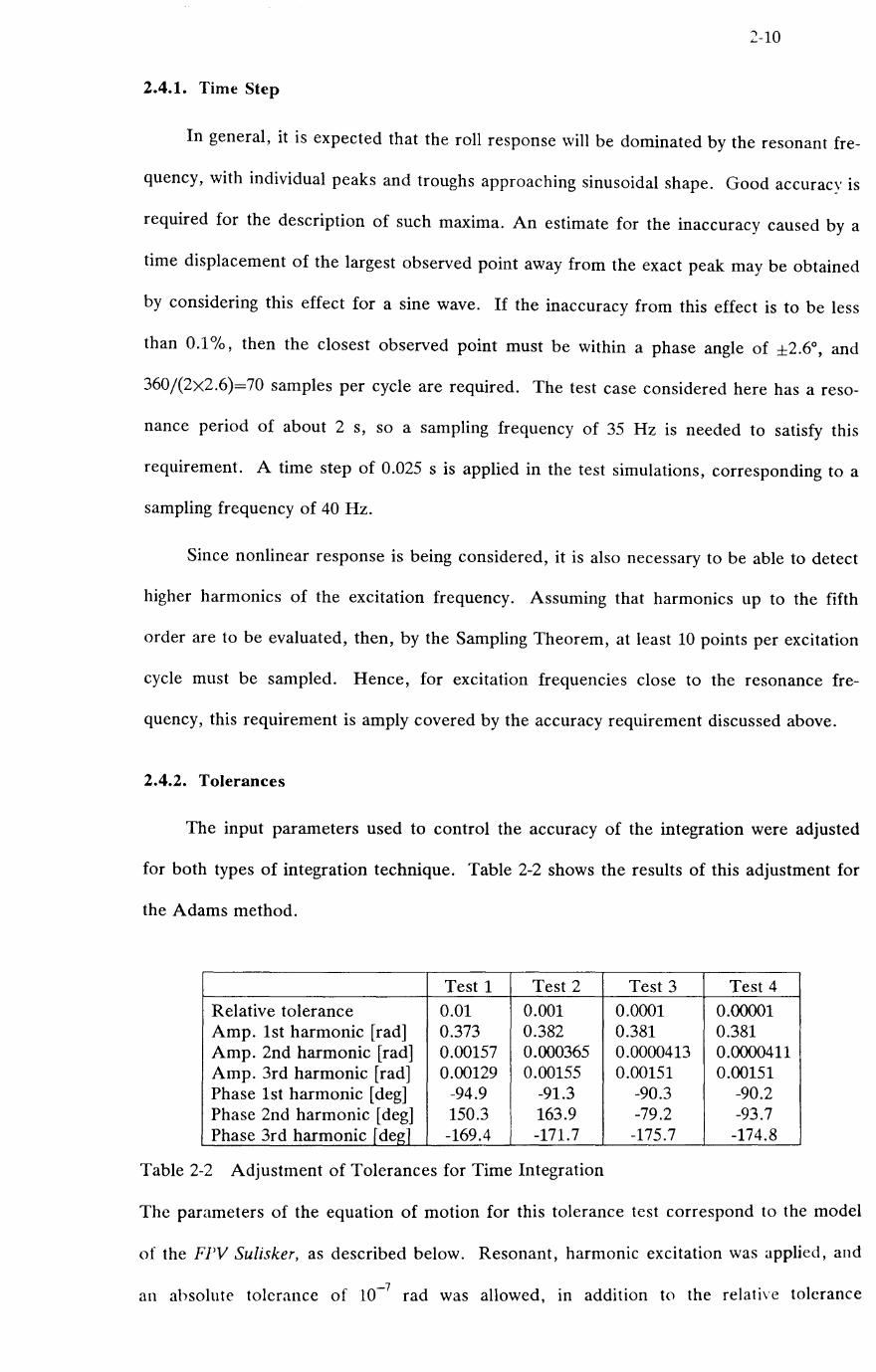
Relative tolerance 0.01 0.001 0.0001 0.00001 Amp. 1st harmonic [rad] 0.373 0.382 0.381 0.381 Amp. 2nd harmonic [rad] 0.00157 0.000365 0.0000413 o . 0000411 Amp. 3rd harmonic [rad] 0.00129 0.00155 0.00151 0.00151 Phase 1st harmonic [deg] -94.9 -91.3 -90.3 -90.2 Phase 2nd harmonic [deg] 150.3 163.9 -79.2 -93.7 Phase 3rd harmonic r deg 1 -169.4 -171.7 -175.7 -174.8
Table 2-2 Adjustment of Tolerances for Time Integration
The parameters of the equation of motion for this tolerance test correspond to the model
of the FPV Sulisker, as described below. Resonant, harmonic excitation was applied, and
an absolute tolerance of 10-7 rad was allowed, in addition to the relative tolerance
2-11
specified in Table 2-2. Harmonic analysis was applied to the simulated roll response, to
provide the tabulated results. The accuracy provided by test 3, with a relative tolerance of
0.0001 is considered satisfactory.
Note that the roll response is dominated by the fust harmonic, but there is also an
identifiable third harmonic present, while the second harmonic is insignificant.
2.5. Some Simulation Results
The following simulation results are all obtained using coefficients in the equation of
roll motion for a model of the FPV Sulisker. as described in appendix D. Coefficients for
the model in the series 1 configuration are used, and the damping coefficients are based on
the results of forced rolling tests near resonance, at a frequency of 3.2 rad/s. The coeffi-
cients are given in Table 2-3. Slightly different inertia and restoring coefficients are used in
the irregular wave simulations, as compared to the actual model data, in order to be con-
sistent with the calculated exciting moments.
Table 2-3
Linear damping Dl 0.512 Quadratic damping D) 3.43 Linear damping Bl 1.47 Cubic damping B, 2.54
Simulation type: Decay and harmonic
Roll inertia A 6.94 Restoring Coefficient C 71.97 Natural frequency w" 3.22
Coefficients for roll motion simulations, based on a model of the FPV Sulisker.
2.5.1. Simulation of Roll Decay
Nms/rad Nm(s/rad)2
Nms/rad Nm(s/rad1
3
Irregular waves
7.40 kgm 2
71.57 Nm/rad 3.11 rad/s
Results of two simulated decay tests are presented, corresponding to the two different
damping models; viz. linear plus quadratic damping, and linear plus cubic damping. Both
decay tests start from an initial roll angle of 0.4 rad and zero roll velocity. The resulting
time series are shown in Fig.2-5 and Fig.2-6. The damping effect due to the two damping
models should be fairly equivalent, since the coefficients of both models are obtained by
estimation from the same set of forced rolling tests, and both models show a fairly good fit
to this data in Fig.J of appendix D. However, there is a definite differcnce in the thc roll
motion shown in Fi~.~-S and Fi~.2-6. \Vhile thc initial parts of the decay rccords are \'cry

Fig.2-5
Fig.2-6
VI Z <I: ..... Cl <I: IX:
w -l l!l Z <I:
-l -l 0 IX:
.3
.2
.1
- . 1
-.2
-.3
-.4 0 5 10 15 20 25 30 35
TIME SEC
Roll decay simulation for FPV Sulisker model with linear plus quadratic damping .
VI Z <I: ..... Cl <I: IX:
w -l l!l Z <I:
-l -l 0 a:
. 3
.2
.1
-.1
- 2
-.3
-.4 0 5 10 15 20 25 30
TIME SEC
Roll decay simulation for FPV Sulisker model with linear plus cubic damping.
2-12
J I
40 45 50
50
2-13
similar, the latter part of the decay record due to the linear plus cubic damping model
shows a more rapid attenuation of the roll motion. This behaviour might be expected from
comparison of the magnitudes of the two linear damping coefficients, which dominate the
decay rate at small amplitudes. The visual impression of the difference is amplified by the
decay process, which effectively integrates the effect of the difference in damping over the
preceding roll cycles.
The tolerances applied in the numerical integration of of these two decay records
were reduced by a factor of 100, compared to thoses specified in section 2.4.2. This was
done to provide increased accuracy for a numerical test of the damping coefficient estima
tors, described in section 6.3.
2.5.2. Roll Response to Harmonic Excitation
A harmonic excitation signal is shown in Fig.2-7, illustrating the initial taper applied
to the first 20 s of the signal, in order to reduce the transient response. The corresponding
simulated roll response is shown in Fig.2-8, with a steady state attained after about 50 s of
simulation. Harmonic analysis (q.v. chapter 5) is applied to the steady roll response to
obtain the harmonics of the response. The results of several such simulations are given in
Table 2-4, and in Fig.2-9. Only the third harmonics are included in addition to the first
harmonics in Table 2-4, since the other harmonics (up to order 5) were even smaller. The
results at a frequency of w=3.2 rad/s, close to resonance, show a gradual change in the
phase angle as the response amplitude increases, due to the nonlinear increase in damping.
The relative amplitude of the third harmonic also becomes slightly larger, though there is
still very little difference between the largest roll angle in each simulation, and the ampli
tude of the fITst harmonic. The nonlinearity of the roll response at the frequency of w=3.2
rad/s is apparent in Fig.2-9, while linearity is displayed at the other 3 frequencies, further
away from resonance.
Most of the simulations with harmonic excitation employ the linear plus cubic damp
ing model, but a few results are also included in Table 2-4 for the linear plus quadratic
damping model. Good agreement between the roll response with the two damping models
is obtained for an excitation amplitude of -+ Nm. As the excitation increases above this

2-14
.5 I (T (I ['
.4 l-
x:: .3 -z
.2 l-
. 1 ~
0 1\ v ~
- . 1 I-~ z w x:: 0 -.2 x:: l-t!)
z ..... ~ ..... -. 3 ~ u x W
...J
...J - . 4 I-0 a:
-.5 I II "
I
0 10 20 30 40 50 60 70 80 90 100
TlME SEC
Fig.2-7 Harmonic excitation signal with amplitude 0.5 Nm and frequency w=3.2
rad/s .
. 10 , , , , -, , , , ,
.08 I-III Z < .... 0 .06 I-< a:
.04 ~
.02 I-
0 11.1'1
v~
- .02 I-
- .04 I-
w ...J -.06 ...-t!)
z < ...J ...J - .08 I-0 a:
-.10 , I I I I I I I I
0 10 20 30 40 50 60 70 80 90 1130
TIME SEC
Fig.2-8 Simulated roll response to excitation signal in Fig.2-6, with linear plus cubic
damping.

Excitation Maximum Roll response harmonics
Roll 1st Frequency Amplitude
Angle Amplitude Phase frad/sl [Nml [radl frad] [°1
Linear plus cubic damping 3.2 0.5 0.0940 0.0940 -80.4
" 1.0 0.158 0.158 -82.0 " 2.0 0.240 0.240 -84.1 " 4.0 0.338 0.338 -86.1 " 8.0 0.455 0.455 -88.0 " 12.0 0.536 0.534 -89.1 " 16.0 0.599 0.597 -89.8 " 20.0 0.652 0.649 -90.4
1.0 4.0 0.0615 0.0615 -1.3 " 8.0 0.123 0.123 -1.3
2.0 4.0 0.0906 0.0903 -4.0 " 8.0 0.181 0.180 -4.4
4.0 4.0 0.102 0.101 -169.7 " "- 8.0 0.200 0.197 -164.9
Linear plus ( uadratic dam ping 3.2 4.0 0.340 0.340 -86.0 " 8.0 0.492 0.491 -87.3 " 16.0 0.707 0.706 -88.4
Table 2-4 Simulation results with harmonic excitation, based on a model of the FPV Sulisker .
. 40
.35
.30
.25
.20
-0 .15 c(
a: -
w .10 0 :::> f-..... ...J 0- .05 2: c(
...J
...J 0 a: eJ
I I
I
I
0
/
"
/ /
F
/
/
/ /
/ /
}l /
2
/ /
/
3
/
/ /
EXCITATION AMPLITUDE (NM)
4 5 6
3rd
Amplitude [rad1
0.0000 0.0002 0.0005 0.0014 0.0034 0.0055 0.0075 0.0096 0.0000 0.0002 0.0000 0.0002 0.0001 0.0003
0.0012 0.0025 0.0051
7 8
Amplitudes of roll response to harmonic excitation,
2-15
Phase [0]
-170.8 -162.7 -163.1 -164.5 -166.1 -166.2 -165.8 -165.1 -123.1 -109.0 157.9 92.0
-26.5 -37.4
-163.5 -165.8 -166.3
9
Fig.2-9 simulated for the FPV Sulisker model, with linear plus cubic damping.
10

2-16
level, the deviation in response with the two damping models also increases. In fact, the
highest excitation level used in the experiments on which the damping coefficients are
based was between 4 and 5 Nm, as shown in Fig.3 of appendix D. The damping due to the
two models diverges above this level, leading to the difference in response observed here.
These results show that the mathematical model reproduces the same response
characteristics (a, b) that are discussed on the basis of model tests, in the beginning of sec
tion 1.5. The third characteristic (c); viz. little variation in resonance frequency with roll
amplitude, has not been studied in detail by simulation. However, the results shown here,
and additional simulations that have been carried out, certainly do not indicate any con
tradiction of this behaviour.
2.5.3. Irregular Waves
Rolling in irregular waves has been simulated with a range of significant wave heights,
and a wave zero-up-crossing period of 1.4 s. This period was chosen because the
corresponding peak period of the Pierson-Moskowitz spectrum lies at about 2 s, which is
close to the natural roll period of the ship model. Initially, the simulations were carried
out with a duration of 2400 s, and a sampling frequency of 40 Hz.
Samples of the exciting moment and roll response time histories are shown in Fig.2-
10 and Fig.2-11, with the corresponding spectra in Fig.2-12 and Fig.2-13. The narrow
banded nature of the roll response is apparent, while the exciting moment is somewhat
more wide-banded.
The first four cumulants of both exciting moment and roll response have been calcu
lated from the simulations, and are shown in Table 2-5 and Table 2-6, excluding the zero
mean values. It was convenient to use the stationarity test of the time series analysis pro
gram (cf. chp.5) for this purpose, since this also provides some indication of the uncer
tainty of the results. An approximate standard error is provided for each cumulant, confer
the description of the sIn directive in chapter 5. Since the roll exciting moment is
modelled as a Gaussian process, the skewness and kurtosis should be zero, and this is con
firmed by the results in Table 2-5. The linear variation of the standard deviation of the
exciting moment with increasing significant wave height is also apparent (the wave zero-up-
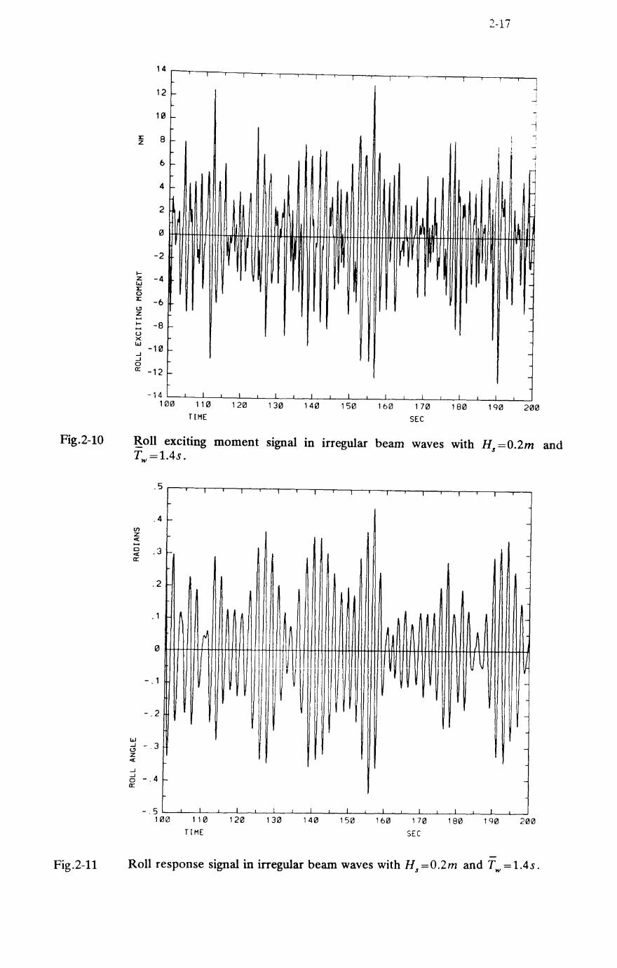
Fig.2-10
Fig.2-11
J: z
I-z w J: 0 x: t!l z ..... I-..... u x w ...J ...J 0 a:
14
12 f-
10 I-
8 l-
6 f-
4 f-
2
0
-2
-4
-6
-8 f-
-10 f-
-12 f-
-14 Hl0
I
I
110
TIME
I
I I
120 130
I T I
I I I
140 150 160
~ ~
~
170
SEC
I
I
180
2-17
~ I
-<
-l
I "1
I i ~ , .J i
~ ,
'-
-
-
-
-
I
200
Roll exciting moment signal III irregular beam waves with Hs =O.2m and Tw=1.4s .
. 5 I T I I I I I I
.4 I--
(J')
z < ..... 0 .3 < -a:
.2 -
. 1
0 f J
- . 1
-.2 ~ ~ ~ U~ V
-
-
w ...J -.3 t!l -z < ...J ...J -.4 0 I- -a:
-.5 I I I I I I I I I
100 110 120 130 140 150 160 170 180 200 TIME SEC
Roll response signal in irregular beam waves with Hs =O.2m and Tw = 1.4s.
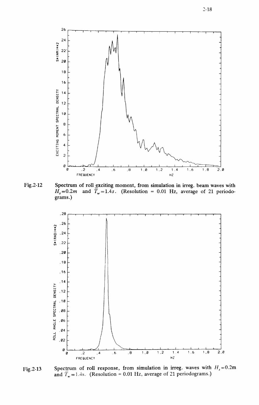
Fig.2-12
Fig.2-13
26
24 C\I It It - 22' J: z -14 If) 2121
18
16
>-~ 14 ..... If) Z I.LJ 0 12 ...J ~ a:: ~ 1121 u I.LJ Q. If)
~ 8
z I.LJ J: 0 6 J:
(!l Z .... 4 ~ .... u X I.LJ 2
II' II' .2 .4 .6 .8 1.13
FRE@UENCY 1.2 1 .4
HZ
1.6
2-18
1.8 2.121
Spectrum of roll ~xciting moment, from simulation in irreg. beam waves with Hs=0.2m and Tw=1.4s. (Resolution = 0.01 Hz, average of 21 periodograms.)
C\I It .. -0 ~ a:: -* If)
>-~ .... If) z I.LJ 0
...J ~ a:: ~ u I.LJ Q. If)
I.LJ ...J (!l Z ~
...J
...J 0 a::
.28
.26
.24
.22
.2121
. 18
.16
. 14
.12
.1121
.1218
.1216
.1214
.1212
121 121 .2 .4 .6 .8
FRE~UENCY
1.0 1.2 1 .4
HZ
1.6 2.0
Spec!!"um of roll response, from simulation in irreg. waves with Hs =0.2m and T .... = 1.4s. (Resolution = 0.01 Hz, average of 21 periodograms.)

Table 2-5
Table 2-6
2-19
Significant Exciting Moment Wave
Height std.dev. [Nm] skewness kurtosis
rml {Iy std.err. K", std.err. KA
0.025 0.412 0.005 0.01 0.01 -0.04 0.050 0.820 0.016 -0.00 0.03 0.05 0.075 1.23 0.02 -0.03 0.02 -0.09 0.100 1.64 0.02 0.00 0.02 0.03 0.125 2.05 0.02 0.03 0.02 0.00 0.150 2.46 0.03 -0.01 0.01 0.02 0.175 2.87 0.05 -0.02 0.03 -0.05 0.200 3.28 0.04 0.00 0.02 -0.01
Excitation Statistics from Irregular Wave SiQIulations, FPV Sulisker Model Series 1, Wave Period Tw=1.4s
Significant Roll Response Wave
std.err.
0.09 0.05 0.03 0.07 0.06 0.06 0.06 0.10
Height std.dev. [rad] skewness kurtosis
rml (Iy std.err. K,,- std.err. KtI
Linear plus cubic damping 0.025 0.0256 0.0005 0.00 0.00 -0.34 0.050 0.0485 0.0014 0.00 0.00 -0.23 0.075 0.0687 0.0018 0.00 0.00 -0.28 0.100 0.0870 0.0022 0.00 0.00 -0.44 0.125 0.104 0.002 0.00 0.00 -0.55 0.150 0.116 0.003 0.00 0.00 -0.38 0.175 0.129 0.004 0.00 0.00 -0.48 0.200 0.142 0.003 0.00 0.00 -0.52
Linear plus quadratic damping
0.100 0.0879 0.0016 0.00 0.00 -0.48 0.200 0.141 0.003 0.00 0.00 -0.55
Response Statistics from Irregular Wave Si~ulations, FPV Sulisker Model Series 1, Wave Period Tw=1.4s
std.err.
0.09 0.12 0.06 0.08 0.05 0.05 0.07 0.07
0.07 0.07
crossing period is held constant).
Nonlinear and non-Gaussian characteristics of the roll response are observable from
the results in Table 2-6. First and foremost from the standard deviation of the roll angle,
which increases at a less than linear rate with the exciting moment. Negative values of kur-
tosis are shown in all cases, with some tendency to increase in magnitude with increasing
excitation. The standard errors associated with the results for kurtosis are large, and
perhaps somewhat too pessimistic, but indicative of the statistical uncertainty associated
with higher order moments and cumulants. Some additional simulations were also carried
out with longer durations, leading to lower levels of uncertainty in the results, and confirm-
ing the behaviour shown here. In particular, the tendency for the magnitude of the kur-

2-20
tosis of the roll response to increase with increasing excitation was brought out more
clearly. The symmetry of the roll motion is reflected by the zero skewness.
Although most of the results were obtained with the linear plus cubic damping model,
a few results are also shown in Table 2-6 for the linear plus quadratic damping model. The
results for the two damping models appear to agree well for these two cases.

3-1
3. A Functional Model for Ship Rolling
Ship roll response to excitation by irregular waves is a stochastic process. Hence,
predictions about the roll motion should be expressed in statistical, rather than determinis-
tic terms. These might include the mean value, standard deviation, and higher order
moments, spectral density, and probability distributions. In the present chapter, ship roll
response to a stationary, irregular sea state is expressed by means of a Volterra functional
polynomial, and this representation is used to obtain some statistics of the roll motion.
Although this analysis does not lead directly to probability distributions for rolling, two
possible candidates for the distribution functions of roll motion and roll extrema are also
discussed.
3.1. Linear Systems Theory
Analysis by techniques employing Volterra functional polynomials may be viewed as a
generalisation of the techniques used in linear systems analysis. A brief summary of some
of the relationships involved in linear systems theory is, therefore, included here as an
introduction to the Volterra functional techniques. This section supplements the introduc-
tion in section 1.6 with some of the equations involved. Price and Bishop (1974) give a
more comprehensive exposition with seakeeping applications, while Newland (1975)
focuses on applications to random vibrations.
In the present case, a convenient starting point is a linear, one degree of freedom,
differential equation for rolling
Ay(t) + B j(t) + Cy(t) = x(t) (3.1)
where y (t) is the roll angle, A, B 1 and C are linear inertia, damping and restoring coeffi-
cients respectively, and x (t) is the exciting moment. A and B 1 may be frequency depen-
dent. A, B l' and C are time invariant. A includes both dry inertia and added maS3. This
equation corresponds to equation (1.11), with omission of the nonlinear damping term, and
a slight change of notation.
The complex form of the linear transfer function (frequency response function, or
response amplitude operator G 1) may be obtained by solution of the differential equation
(3.1) for harmonic excitation, giving
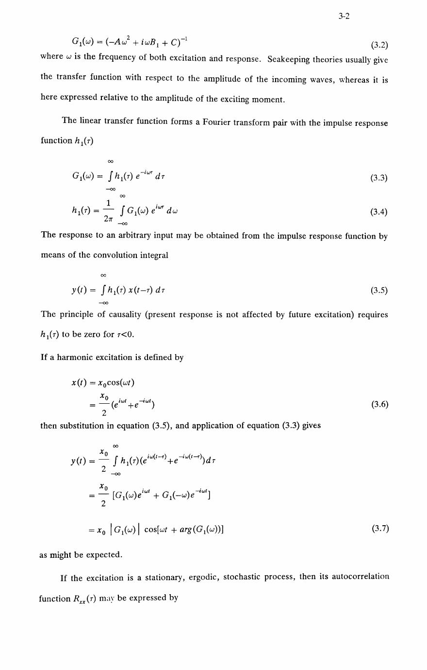
3-2
(3.2)
where w is the frequency of both excitation and response. Seakeeping theories usually give
the transfer function with respect to the amplitude of the incoming waves, whereas it is
here expressed relative to the amplitude of the exciting moment.
The linear transfer function forms a Fourier transform pair with the impulse response
function hI ( 7)
00
(3.3)
00
(3.4) ---<Xl
The response to an arbitrary input may be obtained from the impulse response function by
means of the convolution integral
00
yet) = J hl(7) X(t-7) d7 (3.5) ---<Xl
The principle of causality (present response is not affected by future excitation) requires
hl(7) to be zero for 7<0.
If a harmonic excitation is defined by
x(t) = xocos(wt)
xo. . = - (e lwt +e -Iwt)
2
then substitution in equation (3.5), and application of equation (3.3) gives
00
yet) = Xo J hl(7) (e iw(t-r)+e-iw(t-r»)d7 2
---<Xl
xo. . )
I wt G ( ) -I wt ] = - [G 1 (w e + 1 -w e 2
= Xo I G1(w) I cos[wt + arg(G1(w»]
as might be expected.
(3.6)
(3.7)
If the excitation is a stationary, ergodic, stochastic process, then its autocorrelation
function Rxx(7) may be expressed by
T
2
1 Rxx(r) = lim - J x(t) x(t+r) dt
T-+oo T -T
2
3-3
(3.8)
where r is a time lag. The (two-sided) spectral density S=(w) forms a Fourier transform
pair with the autocorrelation function
00
(3.9) -00
00
(3.10) -00
These two equations are known as the Wiener-Khintchine relations. It may be shown that
the response spectrum is obtained from the input spectrum and the transfer function by
2
Syy(w) = I G1(w) I Sxx(w) (3.11)
The variance of the response is given by the area under the spectrum
(3.12)
where fly is the mean response, which may be taken as zero for a linear system when the
mean excitation is zero. (The presence of the 1/(211") factor here is due to its location in
equations (3.9) and (3.10).)
The cross-spectral density Sxy (w) between input and response is defined in terms of
the Fourier transform of the cross-correlation function, and may be obtained from
(3.13)
If the input is a stationary, Gaussian or normal stochastic process, then the response
Y from a linear system will also be Gaussian, and completely specified in the probability
domain by its first two moments; i.e. the mean fly and variance O":y. The probability density
function of the normal distribution for a random variable Y is defined by
1 {_(Y_fly )2 } f y(y ;fly ,O"yy) = v:?: exp 2
O"yy 211" 20"yy
(3.14)
Furthermore, if the response is narrow-banded, then the response extrema Y. (i.e. maxima
or minima of the process) are distributed according to the Rayleigh distribution, with pro-
babilitv density gi\'cn by . .. ..... ' ~

3-.+
f (y. ) _ 2y -~l/Y/: y. ,7]y - 2 e (3.15)
7]y
where 7]y=Uyy V2 is the parameter of the distribution. The mean period between maxima
(or minima) of the process is equal to the zero-up-crossing period, which is given by
00 00
(3.16) o o
3.2. A Functional Polynomial for Nonlinear Rolling
The Volterra functional series, giving the response yet) of a system to an excitation
X(t), may be written
00
yet) = J hl(T)X(t-T) dT -00
00
-00
00
-00
(3.17)
where the functions hI' h 2' ... are called the Volterra kernels of the system. It may be
seen that the first term in the series is identical to the response of a linear system, given in
equation (3.5); i.e. the first order Volterra kernel is identical to the impulse response func-
tion of a linear system. Schetzen (1980) provides an excellent presentation of the Volterra
functional series, and related techniques of analysis. Schetzen states that this series may
be used to represent the output of a nonlinear system which is time invariant and has a
stable first order kernel. Furthermore, the Volterra series solution of a nonlinear differen-
tial equation is stated to be a perturbation about the linear solution. Hence, convergence
of the series may only be expected for a limited range of solutions in the vicinity of the
linearised equation.
Truncation of a Volterra senes after a limited number of terms leads to a system
representation which is termed a Volterra functional polynomial. A functional polynomial
is derived in appendix C for nonlinear ship roll response, described by the differential
equation
(~.lX)
where ;\ cubic daIl1pin~ tcrlll has been introduced III addition to the terms III the linear

3-5
equation (3.1). Following Vassilopoulos (1967) and Dalzell (1976), the linear plus cubic
damping model is preferred to the linear plus quadratic model in the present context,
because this allows useful expressions for the higher order transfer functions to be derived.
While the quadratic damping term is not analytic (it cannot be expressed as a power series
about the origin), the cubic damping term is analytic in any finite range. Hence, advantage
may be taken of a theorem given by Rugh (1981), which guarantees that there is a conver-
gent Volterra system representation for all sufficiently small inputs, if a solution to an
unforced linear-analytic state equation for the system exists.
The analysis in appendix C shows that all terms of even order are zero for this sys-
tern, due to the symmetric nature of the terms in the differential equation (3.18). In order
to obtain some improvement on a linearised solution, with a minimum of complexity, the
series is truncated after the third order term. The basic results of the functional polyno-
mial solution are the linear and cubic transfer functions, obtained in equations (C.24) and
(C.23) of appendix C. The fifth order transfer function is also given in equation (C.28).
These results correspond to those derived by Dalzell (1976) by a slightly different
approach, and including a nonlinear restoring term in addition. The linear transfer func-
tion of the functional polynomial is identical with the result in equation (3.2), while the
cubic transfer function is given by
(3.19)
Note the symmetry of the cubic transfer function G3; i.e. the order of the arguments is
interchangeable. If the linear transfer function shows a sharp resonance near wn = V C /A ,
then equation (3.19) indicates that the cubic transfer function G 3 will have a number of
very sharp local maxima, with global maximum near (wn,wn,-wn)·
The system response to a single harmonic excitation, as in equation (3.6), may now
be derived from equation (3.17), with a little more effort than in the linear case given in
equation (3.7), to obtain

3-6
+ G ( ) 3iwt G ( -3iwt} 3 W,W,W e + 3 -W,-w,-w)e (3.20)
This includes the linear response term of equation (3.7), with an additional term at the
same frequency, and a third harmonic term.
Under excitation by a stationary, Gaussian, stochastic process, with zero mean value
and spectral density Sxx(w), the response spectrum is obtained in equations (C.39), (C.43),
and (C.4S), which are reproduced in the following.
Syy(W) = Syl(w)+Syiw) 2
Syl(W) = 1 G1(w) 1
00
3 2 2
·11--iB3wG1(w) J w: 1 G1(w1) 1 Sxx(w1)dw11 Sxx(w) 7r o
2 2
·1 G1(w1) 1 ·1 G1(w2) 1 ·Sxx(w-wl-w2)Sxx(wl)Sxx(w2)dwldw2
(3.21)
(3.22)
(3.23)
Note that both input and response spectra are real, even functions, extending from -00 to
00. Hence, ordinates of one-sided spectra are given by twice the ordinates of the two-sided
spectra for positive frequencies. This result for the roll response spectrum also
corresponds with the result obtained by Dalzell (1976). The above expressions show that
input at one frequency can lead to response at more than one frequency. Thus, the fre-
quency components of the scalar response spectrum will be correlated to some extent.
As in the linear case, the variance of the roll response may be obtained from the area
under the response spectrum
00
2 1 Cfyy = - J[SYl(W)+Sy3(W)]dw (3.24)
7r 0
Bedrosian and Rice (1971) have given expressIOns for the first four cumulants of the
response. Since the even order kernels are zero in the present case, the odd order cumu-
3-7
lants are also zero. Their result for the kurtosis is given by
00
Ky. ~ + {24 J J J G,(W,)G,(W2)G,(W,;)G,( -w,,-w,,-W3)
(Jyy --00
00
--00
(3.25)
Higher order cumulants and cross-cumulants between roll angle and roll velocity can, in
principle, be obtained in a similar manner. Hence, it is possible to determine the probabil-
ity structure of the non-linear roll response and the roll extrema by this method. However,
the computational effort involved appears to be large.
3.2.1. Numerical Evaluation of Roll Response Spectrum
The roll response spectrum is composed of the two terms defined by equation (3.22)
and equation (3.23). The first of these two terms is fairly easily evaluated, noting that the
integral in equation (3.22) is independent of the response frequency w, and corresponds to
the variance of a purely linear roll velocity. The infmite extent of the integrals does not
pose too much of a problem either, since each 1 G1(w) 12 term is of order w -4 for large w,
and the excitation spectra S.rx(w) may also be expected to rapidly tend to zero. However,
the integral in equation (3.23) requires more care.
This integral may be split into an inner and an outer integral, such that
00
(3.26)
--00
where I1(w,w
1) is the integrand of the outer integral, expressed by
00
(3.27)
--00
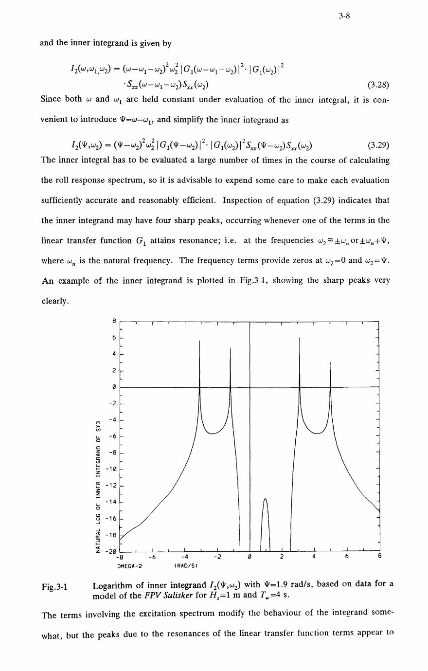
and the inner integrand is given by
[2(W,W1,W2) = (W-W1-W2)2 W; IG1(W-Wl-W2)12·IG1(W2)12
. Sxx(W-W1-W2)Sxx(W2)
3-8
(3.28)
Since both wand w1 are held constant under evaluation of the inner integral, it is con-
venient to introduce \II'=w-w1, and simplify the inner integrand as
(3.29)
The inner integral has to be evaluated a large number of times in the course of calculating
the roll response spectrum, so it is advisable to expend some care to make each evaluation
sufficiently accurate and reasonably efficient. Inspection of equation (3.29) indicates that
the inner integrand may have four sharp peaks, occurring whenever one of the terms in the
linear transfer function G1 attains resonance; i.e. at the frequencies w2 ::::; ±wn or±wn+\II',
where wn is the natural frequency. The frequency terms provide zeros at w2=O and w2 =\11'·
An example of the inner integrand is plotted in Fig.3-1, showing the sharp peaks very
clearly.
Fig.3-1
8
6
4
2
0
-2
('I') -4
>-r.n ~ -6 0
0 z -8 «I: a::
" w -10 I-z ....
a:: -12 w z z .... ~
-14 0
" -16 0 ...J
...J cc -18 a:: ::J l-cc z -20
-8 8
OI1EGA-2 (RAO/S)
Logarithm of inner integrand [2(\11' ,w2) with \11'=1.9 rad/s, based on data for a model of the FPV Sulisker for Hs=l m and T..,=4 s.
The terms involving the excitation spectrum modify the behaviour of the integrand somc-
what, but the peaks due to the resonances of the linear transfer function terms appear to

3-9
be the dominant feature, providing the linear damping is light. Accurate numerical evalua-
tion of the inner integral clearly requires many evaluations of the inner integrand in the
vicinity of the peaks, while fewer evaluations are required over the remainder of the range
of w2• Accordingly the full range of w2 is split into a number of segments, taking care of
the various possibilities arising when some of the peaks or zeros coalesce as \II varies. The
segments are integrated separately, using a Romberg integration algorithm to ensure a
specified accuracy, and the inner integral is obtained as the sum of the integrals for each of
these segments.
A similar segmentation scheme is used in the evaluation of the outer integral, smce
equation (3.27) indicates that there will be a peak in the outer integrand at wI ~ ±wn
and a
zero at wI =0.
3.3. The Edgeworth Probability Distribution
According to linear systems theory, a Gaussian input process to a linear system will
yield an output which is also Gaussian. However, rolling is being treated as a non-linear
response, so it is not necessarily a Gaussian process. In fact, the results of chapter 6 indi-
cate that rolling experiences a non-linearly increasing damping. Intuitively, this should lead
to lower probability for large roll angles than indicated by a normal distribution, while the
probability for roll angles near zero is little changed. Hence, a probability distribution is
sought, which can take the normal form for some values of its parameters, and which can
also deviate from the normal by reduced probability for large values of its argument. The
Edgeworth probability distribution is one such distribution which has already been applied
to other types of seakeeping responses by Nordenstr0m (1972), Vinje (1976), and Jensen
and Pedersen (1980). Furthermore, the cumulants of a random variable, form the parame-
ters of an Edgeworth distribution, if and when this distribution is appropriate, and cumu-
lants for ship rolling have been obtained above to the 4th order.
The Edgeworth distribution is discussed by Cramer (1946), Ord (1972), and Kendall
and Stuart (1977). Its probability density function may be written
, X-Jl
!.,-(x;P.cr,t':,.I\"4'· .. . K,) = <IJ(--)'(l + ~gJ (J ;=3
3-10
where Jl is the mean, (J is the standard deviation, the "'i' (i =3,4, ... ,r) are standardised
cumulants, gi are the terms of the Edgeworth series expansion, (r-2) is the order of the
expansion, and <I>(u) is the standardised normal density function, given by
X-Jl 1 2 <I>(u) = <1>(-) = -e -u /2
(J \12; (3.31)
where u=(x-Jl)/(J is the standardised variate. The "zero" order Edgeworth distribution
corresponds to the normal distribution in the terminology adopted here. If the central
moments of the distribution of a random variable X are defined as
00
-00
then the standardised cumulants are given by
(3.32)
(3.33)
(3.34)
(3.35)
(3.36)
The third cumulant ("'3) is referred to as the coefficient of skewness, and the fourth cumu-
lant ("'4) as the coefficient of kurtosis. Only the first and second cumulants (mean and
standard deviation) of a normal distribution may take non-zero values. The terms of the
Edgeworth expansion are defined by
H j indicates the Hermite polynomial of order i , given by
3 H3(U) = U - 3u
4 ') H 4 (u) = u - 6u ~ + 3
Hj(u) = uHj_1 (u) - (i -1)Hj _ 2(u)
(3.37)
(3.38)
(3.39)
(3.40)
(3.41)
(3.42)
(3.43)
Thc Edgeworth distribution is somewhat similar to the Gram-( ~harlicr Type A distribution.
I10\\'C\Tr. according to Cramer (1946), the Edgeworth series cOIl\'erges more rapidly. and
is therefore to be preferred. :\ first order Fdge\\"orth di-;tributiol1 introduces some

Fig.3-2
3-11
.50
.45 KURTOSIS=-1
.40
.35
.30
.25
.20
.15
>- .10 ~ ~
Vl Z W 0 .05 >-~ .....
~7 ..J ~
CD c:(
CD 0 cr a. -.05
-4 -3 -2 -1 o 2 3 4 ARGUMENT X
Probability density function of a second order Edgeworth distribution, with J..l=0, 0-=1, K 3=0, and different values of K 4 •
asymmetry in the distribution if the skewness is not zero. Fig.3-2 illustrates how the Edge-
worth distribution to 2nd order varies from the normal distribution, which has zero kur-
tosis. Note that some values of the parameters may lead to negative probability densities,
which are theoretically inadmissible. This undesirable effect is due to truncation of the
series. A 2nd order Edgeworth distribution with zero skewness will have positive density
for kurtosis in the range 0<K4<2.4, according to Ord (1972). For roll angles, a distribution
is required with less area under the tails of the probability density function than is the case
for the normal distribution. Fig.3-2 shows this to correspond to negative kurtosis, which
will lead to negative probability densities in a second order Edgeworth distribution. A
magnified view of these negative densities is shown in Fig.3-3 and Fig.3-4 shows that the
problem may be reduced in a fourth order Edgeworth distribution with positive sixth cumu-
lant. However, it may be necessary to include a considerable number of terms in the
Edgeworth distribution to completely eliminate the negative densitiest. The coefficient
t Recently. Winterstein (1987) has proposed an alternative to the Edgeworth distribution, which does not suffer from the problem of negati\'e densities. while still making use of both Hermite polynomials and cu
mulants.

Fig.3-3
Fig.3-4
>t-..... (f)
z w o
3-12
.0050 r-r--r-T, 1\ T--r-~'1---'-~'-r-o-~:::!:. -=-~--=:::r-'i(ljffi~~i'""l
.0045 \
.0040
.0035
.0030
.0025
.0020
.0015
.0010
.0005
\ \ \ \ , \
\ \ \
\ \
\
\
\ \ \
0~--------~----~~~ ______ ~~===-~ __ ~~ \ - - - --- - ::-::.. :::-==- -
\ \
3.6 3.B 4.0 4.2 4.4 4.6 4.8 5.0 ARGUMENT X
Excerpt from a 2nd order Edgeworth probability density, to show negative densities, with p=O, 0'"=1,1\':3=0, and different negative values of 1\':4'
.0010r-.-.-'-~-r~~-r~r-~'-~-r~-'--~r-~'-~-r~~~r-r-> A PA-b- fIJ.
>t-..... (f)
z w o
.0008
.0006
.0004
.0002
~ - .0002 ..... ...J ..... OJ c(
OJ o
KAPPA-b- fIJ.2 KAPPA-6= fIJ.4
a: ~ _.0004L-L-~~~~~~_~-L-L~~L-L-~~-L-L~-J--L-~~~~~~
2.4 2.6 2.8 3.0 3.2 3.4 3.6 3.B 5.0
ARGUMENT X
Excerpt from a 4th order Edgeworth probability density, to show negative densities, with p.=0, 0'"=1, 1\':3=0, "4=-0.3, "5=0, and different positive values
of "6'
values used in Fig.3-3 and Fig.3-4 are comparable to the model test results obtained III

3-13
chapter 7. Odd order cumulants are set to zero in these figures, since these coefficients
primarily affect the symmetry of the distribution.
3.4. The Generalised Gamma Probability Distribution
The same type of argument as used to introduce the Edgeworth distribution for the
continuous roll response, may also be applied to the response extrema; i.e. the nonlinearly
increasing damping may be expected to decrease the probability of large extrema, while not
affecting the probability of small extrema very much, as compared to a linear response.
Hence, a more flexible distribution function is sought, which may approach the Rayleigh
distribution for some parameter values. A generalised gamma distribution is one possible
candidate for such a distribution. Ochi (1976), Andrew and Price (1978), and Gran (1979)
have discussed this distribution, including some applications to ship motion response. The
probability density function may be written
/3 X)..f3 1 { x fJ} /x(x;)",/3,a) = (-) - exp -(-) f().,)a a a
(3.44)
where )." /3, and a are parameters which may be referred to as shape, slope and scale
parameters, respectively. r(.) is the gamma or factorial function.
3.4.1. A Constraint on the Generalised Gamma Distribution
Since a distribution is required which approaches the behaviour of the Rayleigh distri-
bution as the argument approaches zero, this requirement may be utilised to place some
constraint upon the generalised gamma distribution. This constraint may be determined by
expanding both distributions as exponential series, and equating them as the argument
tends to zero. The result is
).,/3=2 (3.45)
Fig.3-5 shows some gamma distributions with this constraint applied. The case ().,=1,j3='2)
corresponds to the Rayleigh distribution. For ).,<1 and /3>2, the upper tail probabilities
are clearly reduced, conforming to the trend expected for rolling. The opposite effect
occurs if ).,> 1 and /3<2. The curves approach each other as the argument tends to zero.
With this constraint, the notation for the probability density simplifies to
;3 x {x <} 1\"(.'(";j1,0) = - cxp -(-y . I'(2/;3)a a Q
(3.46)

Fig.3-5
, ." " ,
.'1 \
.8
.7
.6
.5
.4
.3 >-~ ..... Vl z .2 w 0
>-~ ..... ~ ..... . , CD cC CD a a: 0- " " ARGUMENT X / ALPHA
\
\
\\ \\ \\
\ \ \ , \ \ '\.. '" "" " "-... ..... ~
3-14
'.8 2." 2.2 2.4 2.6 2.8 3.0
Probability density function of constrained gamma distribution, with Q=l, and different values of 13.
A strong similarity to the Weibull distribution may perhaps be apparent, but the two distri-
butions are not identical, as shown by comparison with equation (3.47) which gives the
Weibull density
13' x {x} /x(x;f3',Q') = - (_)",'-1 exp -(-l! Q' Q' Q'
(3.47)
where 13' is the slope and Q' is the scale parameter of the Weibull distribution. The con-
strained gamma and the Weibull distributions are only identical when both reduce to the
Rayleigh distribution, w~th /3=/3'=2. Fig.3-6 is included to show a comparison of cumulative
distribution functions for the constrained generalised gamma distribution and the Rayleigh
distribution in the upper tail region. The two distributions are arranged to have the same
mean square value by setting Q'=Q Vr(4/f3). The difference in the argument approaches
20% at the higher probability levels, giving some indication of the effect of the distribution
functions on predicted roll angles. The value of the slope parameter chosen for this figure
(/3=2.5) corresponds to some of the results obtained for roll in section 7.

Fig.3-6
0.999990
0.999900
0.999000
0.990000
121.9012100121
0.800000
0.700000
0.600000
>- 0.500000 r-...... -l 0.400000 ...... C)
eI: ~ 0.300000 a: Cl.
...... rei: -l :::> :L :::> u 0.100000
---
1.0e-01 ARGUMENT
CNSTR. GAMMA RAYLEIGH
/ /;/ II
VI I;
~
Jill If
j
I I
V
/ 5 1.0e+00
x
3-15
/ II I
5
I
Ii.
II I I
I ,
I i I
>.... ...J
III
"" III a a: 0..
...J
...J => CD
W ~
1.0e+01
Comparison of constrained gamma and Rayleigh distribution functions, with equal mean square values, parameter a=l, plotted on Weibull probability paper.
3.4.2. Estimation of Parameters
Some difficulty has previously been experienced in estimation of the parameters of
the generalised gamma distribution (cf. Ochi (1976». The applied constraint has reduced
the number of parameters from 3 to 2, and should ease this problem. Maximum likelihood
techniques were applied by Mathisen (1983) to develop estimators for the parameters. The
resulting equations are
13 . 2 2 . 2 13 . . 2 . - ~x! +-'I/;(-)~x! +-In(-ijf)ij! --132:(xflnxJ=O n n 13 n 2n n
(3.48)
A ~A P Q = j3iji (3.49)
2n
where all the summations are taken from i=1 to i=n, Xi are observed values, the A notation
is used to emphasise estimated values, and '1/;(.) is the digamma function defined by
d In r(z) 'I/;(z) =
dz (3.50)
The solution for the slope parameter 13 is inconvenient, but can be obtained numerically,
quite economically, provided the number of observations n involved in the summations is

3-16
not too large.
3.5. Some Results with the Functional Model
Coefficients for the differential equation (3.18), appropriate to the model of the FPV
Sulisker, and taken from Table 2-3, are applied in the following.
3.5.1. Visualisation of the Cubic Transfer Function.
Fig.3-7 shows the modulus of the linear transfer function for rolling, as defined by
equation (3.2). The abscissa is given relative to the natural frequency
(3.51)
.22
.20
- .18 :I: z "'-0 . 16 c(
a: -.14
a. .12 ::E c(
f-Z .10 w :I: 0 :I:
t!) .08 z -f--u .06 x w
"'- .04
a. ~ .02 --l I----~ --l
~ 0L-..J'----'---l-..---LJ.---1.--L--L----L-L....l-..L..l.-...L...l.-L=:J~=r::::L::I:::::c::::t:::r:::::::t::::c:±::::d o .2 .4 .6 .81.01.21.41.61.82.02.22.42.62.83.0
OIHENSIONLESS FRE~UENCY OHEGA / OHEGA-N
Fig.3-7 Modulus of the linear transfer function for rolling.
The cubic transfer function is awkward to visualise, since it is complex and has three argu-
ments. The approach adopted here is to show surface and contour plots of the modulus
with the third argument (w 3) held constant. Only positive values of W3 need be considered
since
• Gi -wl'-W2,-w3) = G3 (wl'w2,w3) (3.52)
where the * indicates a complex conjugate. A surface plot is shown in Fig.3-8. The vcrv
"spikey" nature of the cubic transfer function is immediately apparent. In order to obtain

3-17
Fig.3-8 Linear surface plot of the modulus of the cubic transfer function with 03=1.0.
more detail, logarithms to base 10 have been taken of the cubic transfer function in subse-
quent figures, Fig.3-9 to Fig.3-14, showing both surface and contour plots. In these cases,
the function has been truncated at a value of 10--8 Only half of the W1-W2 plane need be
considered since
(3.53)
The w1=w2 axis thus provides a symmetry axIS, and the cubic transfer function is only
shown on one side of this axis. The wI=-w2 axis is normal to the w1=w2 axis. These two
axes are utilised in the figures. They represent a 45 degree rotation with respect to the WI
and w2 axes.
The cubic transfer function is shown for three values of W3 in Fig.3-9 to Fig.3-14. It is
identically equal to zero for w3=0.0. The largest value is apparent in Fig.3-8, Fig.3-11 and
Fig.3-12 where 03=1.0, occurring at 01=02=-1.0. The ridges apparent on the plots follow
lines where one of the G1-component factors of equation (3.19) attains resonance; i.e. for
01 or 02 equal to ±1.0, or 01+02+03=±1.0. (The jagged appearance of these ridges in the
surface plots is due to a weakness in the plotting algorithm.)

Fig.3-9
Fig.3-10
(II
c: I
II ....
c:
3-18
Logarithmic surface plot of modulus of cubic transfer function with °3=0.5.
0.0 r-'---'-'-TTnr'-"IT-'''--Trrn---'-~~n-r-r-~--~
-6.0 L-______ ~ __ -L-L~ ________ -LUL_L __ ~ ____________ ~
-3.0 3.0 0 1 = O2
Logarithmic contour plot of modulus of cubic transfer function with 03=0.5.

Fig.3-11
Fig.3-12
3-19
Logarithmic surface plot of modulus of cubic transfer function with 03=1.0.
N c: I
II ....
c:
-6.0 L-__ ~L-~~-L __ L--L __ ~-L __ L-____ ~ ________ ~
-3.0 3.0
Logarithmic contour plot of modulus of cubic transfer function with 03=1.0.
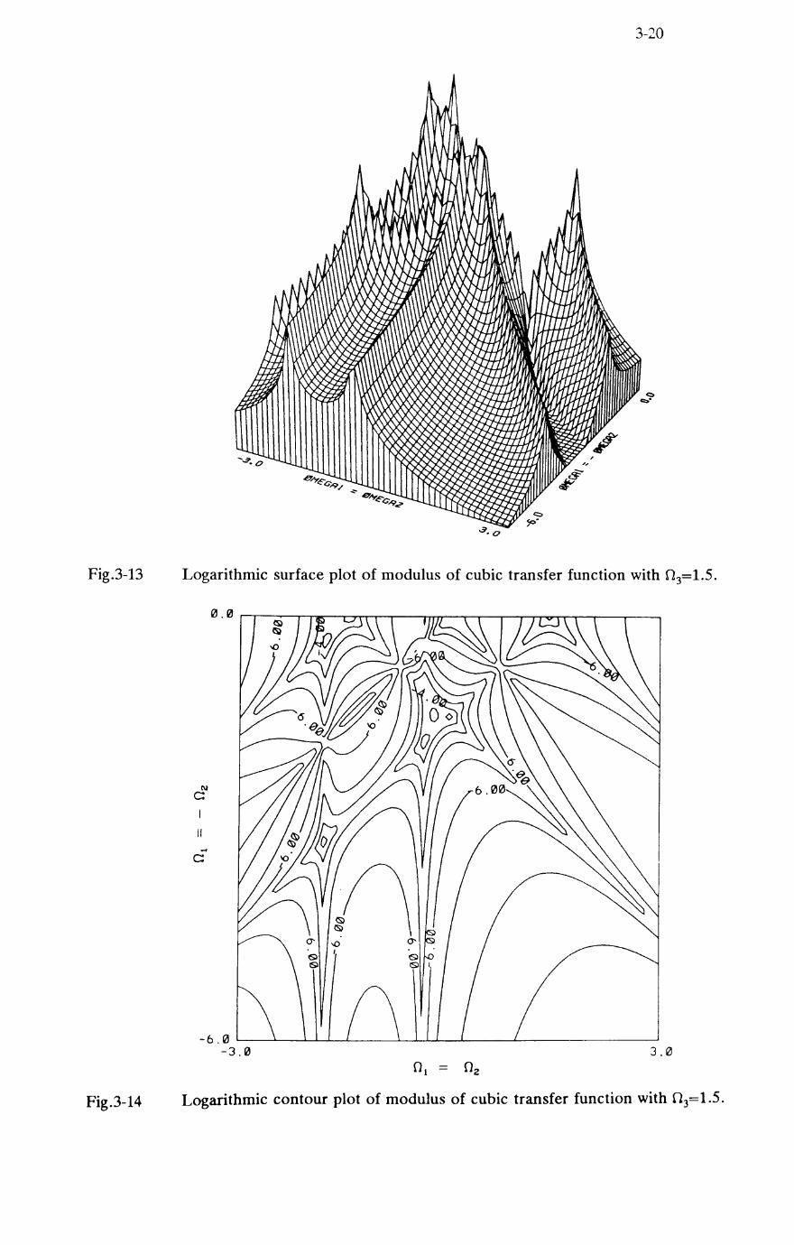
Fig.3-13
Fig.3-14
3-20
Logarithmic surface plot of modulus of cubic transfer function with 03=1.5.
N c: I
II ....
c:
-6.0 L-__ ~ __ ~-L-L ____ ~~~L-~ ____ -L ______________ ~
-3.0 3.0 0 1 = O2
Logarithmic contour plot of modulus of cubic transfer function with 03=1.5.

3-21
It is quite simple to evaluate equation (3.19) for the values of the cubic transfer func
tion. The figures shown here also indicate that this function is quite well-behaved. How
ever, the "spikey" nature of the function requires some care to be taken in integrations
involving this function, as discussed in section 3.2.1.
3.5.2. Response to Harmonic Excitation
The first harmonic of the roll response to sinusoidal input has been calculated from
equation (3.20) for comparison with simulation results in Table 3-1.
Excit.
Freq.
frad/sl 2.0 2.1 2.2 2.3 2.4 2.5 2.6 2.7 2.8 2.9 3.0
Table 3-1
Functional Series Simulation
Linear Cubic Quintic Amp. Phase Amp. Phase Amp. Phase Amp. Phase fradl fdegl fradl fdegl fradl fdegl fradl [degl
.180 -4.4 .1806 -3.8 .1804 -4.5 .1804 -4.4 .1929 -4.3 .1927 -5.2 .1926 -5.2
.207 -6.1 .2077 -4.8 .2074 -6.1 .2073 -6.1 .2259 -5.5 .2253 -7.4 .2251 -7.4
.247 -9.1 .2485 -6.3 .2475 -9.2 .2469 -9.1 .2775 -7.3 .2755 -11.9 .2740 -11.7
.308 -15.6 .3156 -8.7 .3121 -16.2 .3071 -15.8 .3679 -10.5 .3622 -24.0 .3433 -22.3
.392 -31.1 .4435 -13.19 .4435 -39.6 .3480 -32.6 .5611 -17.4 .6732 -72.1 .1229 59.8
.454 -58.2 .7632 -24.9 1.984 -119.3 7.709 79.0
Comparison of first harmonic of roll response obtained from simulation with results from functional series to various orders. Based on data for the model of the FPV Su/isker with excitation amplitude of 8.0 Nm.
Additional results are given in the last 2 columns of Table 3-1, due to inclusion of the fifth
order term of the functional series. At low frequencies the various results agree closely.
As the frequency approaches resonance, the response amplitude increases, the nonlinear
damping takes effect, and the agreement with the simulation results is improved by includ-
ing the cubic and quintic terms of the functional series. However, the results of the func-
tional series in the last two rows of Table 3-1 show an erratic behaviour. This illustrates a
basic property of the Volterra series representation; viz. that it is only convergent for a
certain range of excitation amplitudes. Considering sinusoidal excitation at the natural frc-
quency, the ratio between the first harmonic amplitudes due to the cubic and linear terms
may be obtained from equation (3.20) as
(3.54 )

3-22
Clearly, q must be less than 1.0 for convergence. Also, the range of excitation amplitudes
Xo that provides convergence will be dependent on the relative magnitude of the linear and
cubic damping terms.
Fig.3-15 shows a comparison of results from model tests with results from the func-
tional series. In these tests, the model of the FPV Sulisker was excited with a mechanical
roll moment generator, as described by Schafernaker (1982), designed to produce a
monofrequency, sinusoidal, roll exciting moment .
Fig.3-15
-CI ex: a:: -w CI :::J ~ ..... ...J c.. :s:: ex:
...J
...J 0 a::
. 40r~TI"-.rr,TrT.~~rrrrTTTlII~rr"TI"""rr"""rrrrT<O L.: I A CUBIC SERIES ~UINTIC SER .
. 35 F-__ e ___ M_O_D_EL_T_ES_T_S----..J
.30
.25
.20
.15
.10
. 05
FORCING MOMENT AMPLITUDE (NMI
/
/ /
/
/
e
l' /'
/
e
5.0
Comparison of amplitude of roll response obtained from model tests with results from functional series to various orders. Based on the model of the FPV Sulisker with excitation frequency w=3.5 rad/s.
Again, good agreement is shown for the lowest excitation amplitudes. As the exciting
moment and roll response increase, the model test response falls below the linear predic-
tion. This tendency is followed by the cubic and quintic results of the functional series,
bi.:: less accurately than in the comparison with simulation above. Subsequently, the
results of the functional series diverge, for the largest excitation levels. As the results
begin to diverge, it is apparent from Fig.3-15 that the fifth order term is larger than the
third order term. Hence, a convergence criterion constructed from the ratio of the fifth
and third order terms would bc more restricti\'c than the criterion based on thc third ordcr
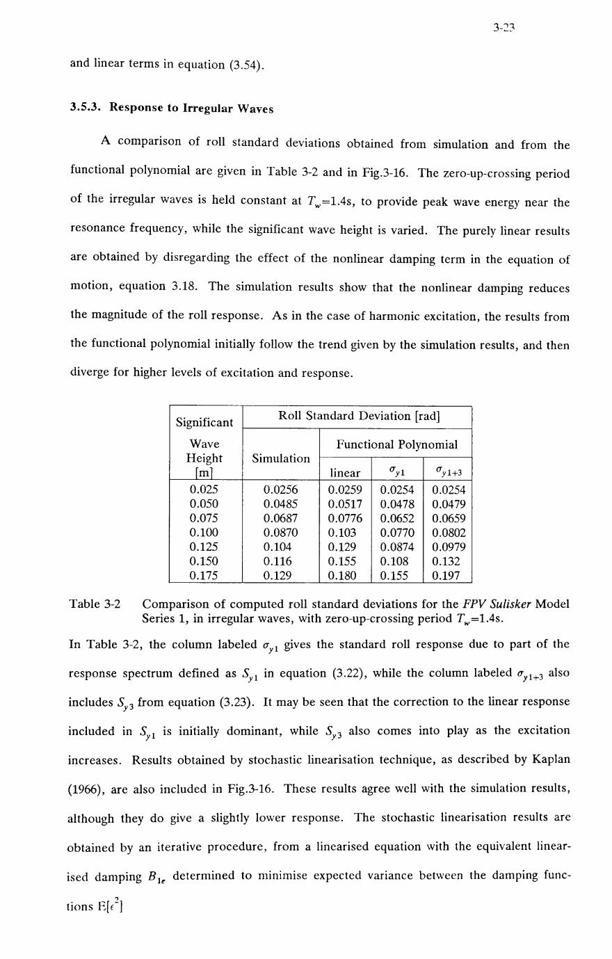
3-23
and linear terms in equation (3.54).
3.5.3. Response to Irregular Waves
A comparison of roll standard deviations obtained from simulation and from the
functional polynomial are given in Table 3-2 and in Fig.3-16. The zero-up-crossing period
of the irregular waves is held constant at Tw=1.4s, to provide peak wave energy near the
resonance frequency, while the significant wave height is varied. The purely linear results
are obtained by disregarding the effect of the nonlinear damping term in the equation of
motion, equation 3.18. The simulation results show that the nonlinear damping reduces
the magnitude of the roll response. As in the case of harmonic excitation, the results from
the functional polynomial initially follow the trend given by the simulation results, and then
diverge for higher levels of excitation and response.
Table 3-2
Significant Roll Standard Deviation [rad]
Wave Functional Polynomial Height Simulation
rml linear O'Y1 O'y 1+3
0.025 0.0256 0.0259 0.0254 0.0254 0.050 0.0485 0.0517 0.0478 0.0479 0.075 0.0687 0.0776 0.0652 0.0659 0.100 0.0870 0.103 0.0770 0.0802 0.125 0.104 0.129 0.0874 0.0979 0.150 0.116 0.155 0.108 0.132 0.175 0.129 0.180 0.155 0.197
Comparison of computed roll standard deviations for the FPV Sulisker Model Series 1, in irregular waves, with zero-up-crossing period Tw=1.4s.
In Table 3-2, the column labeled O'Y1 gives the standard roll response due to part of the
response spectrum defined as Sy1 in equation (3.22), while the column labeled O'YI+3 also
includes Sy3 from equation (3.23). It may be seen that the correction to the linear response
included in Sy1 is initially dominant, while Sy3 also comes into playas the excitation
increases. Results obtained by stochastic linearisation technique, as described by Kaplan
(1966), are also included in Fig.3-16. These results agree well with the simulation results,
although they do give a slightly lower response. The stochastic linearisation results are
obtained by an iterative procedure, from a linearised equation with the equivalent linear-
ised damping B Ie determined to minimise expected variance between the damping func-
')
tions E[ (-]

Fig.3-16
3-24
.20
- -- -.18 - -
-----
.1 b
.14
.12
.10
-0 cc .08 a: -~
5 .0b -f-cc -> w 0 .04 0 a: cc 0 Z cc .02 f-(/)
..J
..J 0 a:
.20 SIGNIFICANT WAVE HEIGHT HS IHI
Comparison of roll standard deviation from simulation, functional polynomial and stochastic linearisation for the FPV Sulisker Model Series 1, in irregular waves with zero-up-crossing period Tw=1.4s.
(3.55)
where Z is the Gaussian response process obtained as an approximation for the actual
non-Gaussian roll response Y.
Two examples of response spectra underlying the standard deviations discussed above
are given in Fig.3-17 and Fig.3-18. A. significant wave height of Hs=O.05m applies in Fig.3-
17, where it may be seen that the response spectrum due to the third order functional poly-
nomial agrees' well with the simulation result. A significant deviation from the purely
linear result is also apparent. The excitation level is increased in Fig.3-18, with Hs=O.lm,
and considerable deviation is apparent between the third order functional polynomial
result, and the simulation result near the resonance frequency.

Fig.3-17
Fig.3-18
" '"'1--'- --::-
.060
d \ -- t. L INEAR+CUBIC .055 I \ - - - - Jl LI NEAR ONLY , \
I \
.050 .. I f
.045
-N .040 I "-N ~ ~ .035 0 ex: a:: -
.12130
~ .025
I-
Ul z .12120 w 0
~ ex:
.015 a:: I-u W Cl. Ul .12110 w ~ (!) z .005 ex: ~ ~ 0 a:: 0
.40 .42 .44 .46 .48 .5121 .52 .54 .56 .60 FREC»UENCY 1HZ)
Comparison of roll spectra from simulation and functional polynomial for the FPV Sulisker Model Series 1, with Tw=1.4s and Hs=O.OSm .
. 24 '--'-'--'--'--'--'--.--r-'rw'--'--TO-.--'--r--~~~~~-' ---'--- 0 5 I H
.22
. 20
.18
-N .16 I "-N ~ ~
o ex: a::
.14
.12
~ .10 I-..... Ul
~ .08 o ~
~ .06 Iu W Cl. Ul .04 w ~ (!)
~ .02 ~ ~
I I
Ii I
d \ I \
" \ I \ I .. f \ I \
I \ If
\ ~
t. LINEAR+CUBIC Jl LINEAR ONLY
~ 0 ~~~Y:~_~~_~~L--L_L--L_L-~_~~_~~_-L~~-L~ .40 .42 .44 .46 .48 .50 .52 .54 .56 .60 FREC»UENCY (HZ)
Comparison of roll spectra from simulation and functional polynomial for the FPV Sulisker Model Series 1, with Tw=1.4s and H s=O.10m.

3-26
. In .the numerical evaluation of the integrals for the functional polynomial, the follow-mg relatIve accuracies were specified to the Romberg integration algorithm:
0.001 for integral part of Syl in equation (3.22) 0.01 for outer integral of S 3 in equation (3.26) 0.002 for inner integral of .s; 3 in equation (3.27)
Slightly higher accuracy was specified for the inner integral, than for the outer integral.
Fairly low accuracy for Sy3 was specified in order to reduce computing time, while intended
to be sufficiently accurate for the present comparison. However, about 2 hours of CPU
time (on Vax780 or Sun-3 computers) were still required to obtain results for one response
spectrum at 30 frequencies, based on the functional polynomial. Although the computer
time required could probably be reduced by improving the integration procedures, it
appears that the resources required are of the same order of magnitude as for simulation.
The simulated response spectra shown in Fig.3-17 and Fig.3-18 were calculated with a
resolution of 0.005 Hz, and averaged over 46 periodograms. The sampli~g frequency was
reduced from 40 Hz to 10 Hz in order to provide a long duration signal without increasing
the amount of data to be handled. This was considered to be permissible, since it had
already been ascertained that negligible response was present at frequencies above 2 Hz.
However, further reduction of the sampling frequency was avoided, since it was found to
lead to some reduction in the response standard deviation. If a longer duration response
signal had been obtained, then additional frequency resolution could have been obtained
without increasing the random error, and somewhat improved agreement would probably
have been obtained on the flanks on the spectrum peak in Fig.3-17 and Fig.3-18.

4-1
4. Long Term Distribution of Roll Response
Stationary environmental conditions are assumed to prevail for the determination of
roll response, throughout the other chapters of this work. Some implications of the remo-
val of this restriction are considered in the present chapter. Consider, for instance, a com-
paris on of the roll response of two alternative ship designs. A design which is favourable
in one sea state may well be unfavourable in another sea state. Some way of combining
the response in various sea states is clearly desirable, and this is provided in the long term
distribution of the response. In a sense, this may be seen as a technique of averaging the
response over a set of different sea states. Usually, the entire set of sea states that may be
encountered is taken, and the averaging process takes the probability of occurrence of
each sea state into account. Thus, the long term distribution becomes indicative of the
response expected for the ship lifetime. As such, it is a useful measure for the comparison
of alternative ship designs. There has also been a tendency to incorporate the results of
long term response analyses into design procedures and classification rules (d. Abraham-
sen (1967) and Lersbryggen (1978». However, this tendency applies to hull girder loads
rather than to roll motion and safety against capsize. Apparently, the general level of con-
fidence in the accuracy of roll response calculations under extreme conditions, has not yet
reached a stage where such calculations may replace empirically based procedures for the
evaluation of safety against capsize.
Early work on long term response distributions was done by Jasper (1956) and
Nordenstn~m (1963). More recently, Spouge (1985) and Roberts et al. (1983) have dis-
cussed applications to ship rolling.
4.1. Basic Derivation of Long Term Distribution
It is assumed that the wave environment may be modeled as a piecewise stationary
process, defined primarily by the two random variables, significant wave height H s ' and
zero-up-crossing period of the waves Tw. Their joint probability density function is
denoted f H T (hs,tw)· The rate of change of the wave conditions is assumed to be suffi-:s w
ciently slow compared to the roll response frequency, that effects of a preceding environ
mental state on the response in subsequent states may be neglected. Furthermore, it is

-+-2
assumed that the distribution of roll maxima Z (or minima) conditional on any stationary
sea state, defined by values of significant wave height and zero-up-crossing period, may be
determined. This is referred to as a short term response distribution, since it is condi-
tional on wave conditions which are stationary for a short period of time, perhaps of the
order of one hour. The short term distribution of roll maxima is denoted by
FZIHs,Tw (z Ihs,tw)' Since the roll response is narrow-banded, the zero-up-crossing period of
the roll response may be taken as the mean period between roll maxima T/hs,tw)' which is
also dependent on the stationary wave conditions. It is required to determine the marginal
distribution of the response maxima Fz(z), referred to as the long term distribution, taking
into account all sea states.
D is introduced as the total time duration to be considered, perhaps representing the
design life of the ship. Then the (infinitesimal) duration of any sea state may be expressed
by
(4.1)
The expected number of response maxima in the sea state is given by the duration of the
sea state divided by the mean response period
Tz(hs,tw) (4.2)
The number of response maxima not exceeding a level z is obtained from the product of
the expected number of response maxima in the sea state, and the cumulative probability
Ns(z;hs,tw) = Ns(hs,tw) FZlh t (z I hs,tw) 8 w
D f H T (hs,tw) FZlh t (z I hs,tw) s wsw
--------------------------dhs dtw Tz(hs,tw)
(4.3)
The number of response maxima not exceeding the level z in the long term is obtained by
integrating the short term result over the range of sea states that may be experienced
(4.4)
Finally, the long term probability of not exceeding the level z IS gIven by dividing the
4-3
number of response maxima that do not exceed this level by the total number of response
maxima
N(z) Fz(z) =--
N(oo)
f H T (hs,tw ) FZlh t (Z I hs ,tw )
= Tz J J s wsw dhs
dtw Tz(hs,tw )
(4.5)
where the total number of response maxima, are simply the number of response maxima
below a level which is never exceeded N(oo), and the long term mean response period has
been obtained by dividing the long term duration by the total number of response cycles
(4.6)
The effect of variation in the mean period between response maxima is included in
the above derivation of the long term distribution. This effect was omitted in some early
work on long term distributions, but was included by Battjes (1972) in work on the distri-
bution of wave heights, and by Ochi and Chang (1978) for response. It may well be justifi-
able to exclude this effect when considering the long term distribution of ship rolling, since
the roll response tends to be strongly dominated by the natural roll period. However, it is
important for responses with more variable periods, especially in the case of bow slamming
pressures (cf. Mathisen (1986)).
4.2. Further Aspects of the Long Term Distribution
The derivation above illustrates the basic principles involved in determination of a
long term response distribution, but is otherwise an over simplification. In particular, the
roll response is dependent on the speed of the ship and on the heading angle relative to the
waves. These effects may be incorporated by including them as variables defining the sta-
tionary conditions under which the short term roll response is computed, and in the
domain of environmental variables over which the long term integration has to be carried
out. For instance, let the vector \V be a random variable whose value defines any set of
environmental conditions that a ship may encounter. The components of \ii might include
significant wave height, zero-up-crossing period, ship speed, heading angle, and any other

4-4
relevant factors. A joint probability density function f -p> would then have to be esta
blished for the components of W. Provided the short term distribution of response
Fzrlz I~ could also be determined, the long term distribution from equation (4.5) would
now take the form
f-P> Fzrlz I ~ Fz(z) = Tz J d¢
Tz~ (4.7)
Nordenstr0m and Pedersen (1966) incorporated features of this type into long term
response calculations. They assumed the heading angle of the ship to be statistically
independent of the wave conditions, while the forward speed was modeled as a determinis-
tic function of the wave conditions, based on the expected frequencies of bow slamming
and green water on deck. Spouge (1985) has elaborated this type of approach further,
including allowance for change of course to avoid heavy rolling, and modification of the
wave climate to take account of rough weather avoidance action by the ship's master.
Since a major objective of a long term response calculation is to predict the probabil-
ity of extreme events, it is vital that the distribution of the variables defining the wave con-
ditions gives an accurate description of the severe conditions that lead to such events.
This implies that a probability description based directly on relative frequencies of sea
states from limited numbers of observations is inadequate. The quality of the probability
description should be improved by fitting suitable distribution functions to the data. This
process smooths out random variations in the observed relative frequencies, and permits
careful extrapolation to infrequently observed sea states. A comparison of some available
joint probability distributions for significant wave height and zero-up-crossing period has
been made by Mathisen and Bitner-Gregersen (1988). A combination of a marginal 3-
parameter Weibull distribution for significant wave height, with a conditional log-normal
distribution for zero-up-crossing period is recommended.

5-1
5. Time Series Analysis Program
A computer program has been written to perform the analysis of model test data
described in chapter 7. It has been formulated as a fairly general tool for the analysis of
time series, with emphasis on measured data from wave-induced responses. The program
is named "Timser." The general structure of the program and the associated database is
described in this chapter, together with some details of the algorithms involved in the
analysis procedures.
The primary assumption about the input data to be analysed is that each sequence of
input data contains values of one variable, sampled and digitised at equidistant steps in time.
Such a data sequence is referred to as a time series, or, as a signal. In this con text, time
acts as an index invariable. Other index variables may be substituted for time, provided
equidistant steps are maintained, and the interpretation of the results is modified accord
ingly. In order to investigate the relationship between two variables, the corresponding
pair of time series must be synchronised by means of information about their starting
points, and should have the same sampling frequency.
The program is built up around a database, where input data must be stored prior to
any analysis, and where analysis results may also be stored. The program is structured in a
modular fashion, such that the user may perform any of the available analyses, on any sig
nal in the database. This modular structure is also designed to allow new types of analysis
to be incorporated easily. Emphasis is given to the provision of suitable graphical presen
tations of the time series and the analysis results, in order to ease their interpretation. The
program may be run interactively or in batch mode. Interactive use is ideal for preliminary
analysis, while batch mode is more convenient for the analysis of large amounts of data,
when the choice of analysis procedures and parameters has been made. Each analysis of
data is initiated by a command, referred to as a "directive," using a mnemonic name 3
characters long. A list of the available directives is given in Table 5-1, together with a
brief indication of their purpose. Experience with a similar program, named "SAMPAN"
(cf. Omundsen et al. (1975», has influenced the design of this program. The program
contains 118 routines and about 31,000 lines of Fortran code, of which 46% are explana
tory comment lines. Standard mathematical and graphics library routines are not included

Mnemonic Purpose dbs DataBaSe - general information (text only) edf plot of observed and expected Cumulative Distribution Func. eov direct COVariance or autocovariance function erd moves data from a formatted file (or CaRDs) to database dey calculates roll damping coefficients from a DeCaY test dee downwards or upwards DECimation of a time series dif DIFferentiates a signal. dlt DeLeTes entries from database
dmp DuMPs database arrays on file and prints attributes eng determines envelope process on ENerGy basis using derivative env determines ENVelope process using Hilbert transform fit FIT distribution functions to observed data fit FiLTer and wild point editing gen GENerates sine wave, normal, or uniform random process hlp HeLP - introduction to program or specified directive hrm HaRMonic analysis - Fourier series, not by FFT inf INput Format - detailed explanation (text only) lea Level Crossing Analysis - maxima, minima, peak-to-trough Idr List DiRectives - gives mnemonic and purpose (text only) opn OPeNs existing database, or creates a new one pit PLoT ppp PP-Plot of observed and expected cdf psd Power Spectral Density by FFT rst ReSeT - sets print switches and secondary output unit stn STatioNarity check along sample record tnd deTreNDing tpe moves data from magnetic TaPE to database
Table 5-1 List of directives available in the time series analysis program Timser.
in this sum.
5.1. The Database
The primary function of the database is to store and retrieve a large number of time
series, each of which may hold a large number of sampled data values (up to 100,000 at
present). These functions are to be carried out with a minimum of effort by the user. A
system of numerical keys is used to achieve this. The user refers to the database entry by
means of it's key, while the database routines carry out the related tasks involved in locat-
ing and manipulating the entry on direct access files. Each key is composed of 3 com-
ponents:
• the experiment set number set,
• the experiment number xpm ,
• the reference number ref·

5-3
Logically, set indicates the set of experiments for one object, xpm indicates an experiment
under constant conditions, and ref initially indicates one transducer or data channel. This
logical structure of the database key aligns quite well with typical numbering schemes used
in experimental work. When a signal identified by one value of reference number has been
analysed, the results may be stored at a new value of reference number, while the set
number and experiment number are held constant. Thus, the implication of the reference
number is widened to differentiate between various types of analysis results as well signals
from different transducers. Allowed ranges are: set(l, 2), xpm (1, 999999), and ref (1,
1(0). Up to 30 different values of xpm may be used at present.
Field no. Name Content
1 liattr length in words of aggregate of integer attributes. 2 iset set key 3 ixpm experiment key 4 iref reference no. 5 mrkdlt delete mark for integer attributes
next narray no. of equisized, real, array attributes next iadrch address of first character of aggregate of
character attributes for this entry next iadrre address of first word of aggregate of real
attributes for this entry next idim number of dimensions of real array attributes
next 2 iorigx(l), experiment nos. for data from which present iorigx(2) results have been derived
next 2 iorigr(l) , reference nos. for parent data from iorigr(2) which present data are derived
next idim nwdaxs(i) (omitted if narray=O) number of data-points along axis i of real array attributes
last ienda~ = 999 999 indicating end of aggregate
Table 5-2 Aggregate of integer attributes for one entry on database
Each entry on the database contains a number of different types of information,
referred to as attributes. An attribute may contain one or many data values of similar
type; e.g. a time series may be one attribute of a database entry. A collection of attributes
is termed an aggregate. The database utilises 3 files for separate storage of integer, real,
and character aggregates. The attributes contained in these 3 classes of aggregates, and
associated with every database entry, are listed in Table 5-2 to Table 5-4.
The file addresses defining the locations of the real and character aggregates for one
database entry arc contained in the associated integer aggregate, as indicated in Table 5-2.
In addition, a hierarchy of index tables arc maintained to keep track of the locations

Field no.
1 2 3 4 5
next mchxpm
next nspace next npar
next maxres
next narray
next narray
next idim
next idim
next
next larray
next next larray
last
Name
rlreat rset
rxpm rref
rmrkdl rxpma(i)
-
rdparv(i)
redres(i)
varmin(i)
varmax(i)
of fset(i ,1)
axstep (i ,1)
a rrk ey
5-4
Content length of this aggregate of real attributes in words set key experiment key reference number key delete mark for real attributes experiment attributes, identified by corresponding fields on character file empty spaces for later use values of parameters used by directive generating these attributes (param. mnemonics on char. file) single entity results from directive (identified by corresponding fields on char . file) (omitted if narray=O) minimum value of variate for each array attribute (omitted if narray=O) maximum value of variate for each array attribute (omitted if narray =0) offset of first data-point along axis i of first array (omitted if narray=O) step between points along axis i of first array
until offset and axstep have been given for all arrays (omitted if narray=O) array key for first array. (omitted if narray =0) contains first array (e.g. a time series)
arrkey array key for last array. contains last array
renda~ = 999 999.0 indicates end of aggregate
Table 5-3 Aggregate of real attributes for one entry on database. Current parameters are: mchxpm=5, nspace=10, npar=20, maxres=5.
of the integer aggregates for each entry. These index tables comprise:
• the main index - one for the entire database,
• the experiment set index - one for each set of experiments,
• the experiment index - one for each experiment, within each set.
Separate subroutines are dedicated to manipulations of each type of index, and to each
class of aggregates. The application interface to the database module is through 2 routines
to open and close the database, and 3 routines to fetch or store integer, real and character
aggregates. All manipulations of the indexes and the file addresses are invisible to the
application routines which make use of the database. There is a separate file handling
module located below the database routines, which carries out the actual operations of
reading and writing on the files. The terminology and organisation of this database has
been based on some of the principles advocated by Martin (1977).
5-5
Field no. Name Content 1-6 lchatr length in characters of this aggregate 7-9 chset set key, maximum unique value is '999'
10-12 chxpm experiment key, max. value is '999999' 13-15 chref reference no. key, max. value is '999'
next 3 chmrkd delete mark for character attributes next mchxpm *lchxpm chxpma(i) mnemonics for mchxpm experiment
attributes, with values stored on real file next Idirna dirnam mnemonic for directive generating results
next nspcch *lspace - empty spaces for future use next npar*ldparn dparn (i) mnemonics for directive parameters
next maxres*lchdre chdres(i) mnemonics for single entity results from this directive (values in real file)
next lsettx settxt identifying text for experiment set next lxpmtx xpmtxt identifying text for experiment
next Idirtx dirtxt identifying text for directive next ldate date date and time for input to directive
next (idim+l)*laxnam axnam(i ,1) (omitted if narray=O) axis names for first array on refile
next (idim+l)*laxuni axunit(i ,1) (omitted if narray=O) axis units for first array on real file.
next lcrvtx crvtxt (omitted if narray=O) curve text for first array on real file .
. . .
... etc. until text given for all such arrays, then last 6 chendaf{ = '999999' indicating end of aggregate
Table 5-4 Aggregate of character attributes for one entry on database. The field no. is given in characters, and each entity is arranged to contain a multiple of 3 characters. Current parameters are: mchxpm=5, lchxpm=3, Idirna=3, nspcch=9, lspace=6, Idparn=3, lchdre=6, lsettx=9, lxpmtx=18, Idirtx=30, Idate=15, laxnam=42, laxuni=21, lcrvtx=12, in addition to values given with Table 5-3.
In some cases, an analysis may well yield more than one array of results; e.g. the fit
directive provides both an observed probability density function and a probability density
function for the fitted distribution. This possibility has been allowed for by permitting the
aggregate of real attributes to contain more than one array attribute. Some provision for
multi-dimensional arrays is also present in the database, but this has not been utilised in
"Timser . "
Experience has shown that the considerable effort put into the design and implemen-
tation of the database has been worthwhile. Large amounts of data have been analysed
with very little manual bookkeeping work being needed to keep proper track of the data.
Inclusion of data labels in the database, and their use in automatic labeling of result plots
have helped to avoid confusion in the interpretation of results. Two weaknesses in the
design have sometimes made themselves felt:

5-6
(a) There is no provision to utilise the results of one analysis directive in a second
analysis directive without intermediate storage on the database. When working
interactively, this results in having to wait while some unnecessary data transfer
operations are carried out.
(b) The indexes are not copied from core to the database files until the database is
closed at the termination of a program run. If some error arises during the run, lead
ing to an uncontrolled error termination of the run, then modifications of the indexes
are likely to be lost, and results stored on the database during that run will not be
retrievable.
5.2. cdf Cumulative Distribution Function Plot
Observed and expected cumulative distributions are integrated from the probability densi
ties generated by directive fit and plotted. Linear plots, normal probability paper, Weibull
probability paper, and Gumbel probability paper are available.
For normal probability paper:
the variate axis is linear,
the inverse of the standard normal distribution for the cumulative probability is used
for the ordinate axis.
For Weibull probability paper:
the variate axis is logarithmic,
the ordinate axis is double logarithmic In { -In[l-F(x ) J}. where x IS the variate and
F(x) is the cumulative probability.
For Gumbel probability paper:
the variate axis is linear,
the ordinate axis is double logarithmic, -In[-lnF(x)].
Examples are shown in chapter 7.

5-7
5.3. eov Covariance Function
The autocovariance of one time series or the covariance function between two syn-
chronised time series x j and Y j' j =0,2, ... ,n -1 is calculated. Standard estimators are
used for the mean values and standard deviations. The mean values are extracted from the
series if they exceed 0.001 of the standard deviations. The covariance function Cj
is com
puted by direct calculation
1 k=k
2
Cj = ~Xk'Yj+k' n -I j 1 k=k}
]=-m, ... ,m (5.1)
where m is the maximum number of lag points required (m «n), k1=0 for positive lags
and - j for negative lags, while k2=n-1- j for positive lags and n-1 for negative lags. The
algorithm is taken from Otnes and Enochsen (1978). Only positive lag points are calcu-
lated when the autocovariance is required, and the results for negative lag points are
obtained by symmetry. Note that this procedure does not calculate a circular covariance
function, which would effectively assume that the signals are periodic outside the range of
time values provided. Instead there is a reduction in the number of points that are aver-
aged as the lag length increases. For graphical presentation, the covariance function is
normalised by the standard deviations, to provide the cross-correlation function. An
example of the results is given in Fig.5-l.
5.4. dey Roll Decay Test Analysis
Linear plus cubic, and linear plus quadratic roll damping coefficients are determined using
the methods described in chapter 6 and in appendix D. The input data (on the database)
must be in the form of a descending sequence of positive roll amplitudes, including both
the maxima and minima. If directive lea is used to extract the amplitudes from the decay
time series, then separate arrays for the maxima and minima, as stored by this directive,
are acceptable, otherwise the maxima and minima should be combined into one sequence.
5.5. dee Decimation
This directive allows the sampling frequency of a time series to be changed. The sampling
frequency can easily be reduced by omitting all but the sample points which are spaced at
an increased time interval. However, this may introduce aliasing effects if frequency
1.0
~
~ .8 ...J ...J
~ .6
> W ...J W
lL. a: :> en
.4
.2
~ -.2 w ...... u ;: - .4 lL. w o u
z o ...... I-
-.6
:3 -.8 w a: a: 8 -1.0 en en o a:
5-8
u -1.2~~~~~~~~~~~~-L-L-L-L-L-L-L-L-L-L~~~~~~~ -140 -120 -100 -80 -60 -40 -20 0 20 40 60 80 100 120 140
TIME LAG SEC
Fig.5-1 Cross-correlation between surface elevation and roll angle from experiment 3 of the irregular wave tests in chapter 7.
components are present in the signal at frequencies between the original and the reduced
folding frequencies.
Three possibilities are available for decimation of a series:
(a) Simple downwards decimation without filtering.
(b) Downwards decimation with anti-aliasing filtering.
(c) Upwards decimation by inserting zeros and filtering at the original folding frequency.
The sample period can only be changed by an integer multiplier or divisor in one pass of
the directive. A non-recursive, symmetric, finite impulse response (FIR) filter is used, as
described for the flt directive. An example is given in Fig.5-2, showing how upwards deci-
mation may be used to provide a more precise definition of a sine wave.
5.6. dif Differentiation
The derivative )'i of a time series x j , j=0,1,2, ... ,n-1 is obtained by finite differ-
ence methods (cf. Dahlquist et al. (197'+)). First and second order central differences are
available. Using first order differences, the derivative is given by

Fig.5-2
Fig.5-3
4.0
3.5
3.0
2.5
2.0
1 .5
1 .0
.5
0
-.5
-1 .1£'
-1 .5
-2.0 w > c:r:: :x -2.5 w z ...... If) -3.1£'
498 TIME
5-9
514 516 518 521£' 522 524 526 528 SECONDS
Comparison of an input sine wave with 10 samples per cycle, and the same signal with sampling frequency increased to 100 cycles per second using directive dec.
3
2
I 'l'\
/ I
w I£' > ...... ..... c:r:: > ...... a: w 0 -1 0 z c:C
w > c:C :x
-2 w z ...... If)
-3 I£' 2 4 6 8 10 12 14 16 30
TIME SECONDS
Example of directive dij, showing a sine wave and it's derivative.

5-10
X j+l-X j _ 1 j =1,2, ... ,n-2 (5.2)
where ~ is the sampling interval. The derivatives at the end points of the signal are
obtained by forward or backward differences.
U sing second order differences, the derivative is given by
8(x j+l-X j-l) - (x j+2 -x j-2)
12~ j =2,3, ... ,n-3 (5.3)
The derivatives one step away from the end points are obtained by first order central
differences in this case. An example is shown in Fig.5-3, for an input sine wave with an
amplitude of 3, and 10 sample points per cycle. In this case the second order differences
are a little closer to the exact amplitude of the derivative which is 1.88.
5.7. eng Envelope Process on Energy Basis
The derivative Y j of a time series x j' j =0,1,2, ... ,n -1 is calculated as described for
directive dif. The envelope process Z j is then obtained from
(5.4)
where w is the zero-up-crossing frequency of the input process. This expression for the
envelope process is taken from Madsen et al. (1986). It is most appropriate when the
input process is very narrow-banded. An example is shown in Fig.5-4. The input signal in
this example is fairly narrow-banded, and yet the quality of the envelope is not very good.
s.s. env Envelope Process Using Hilbert Transform
The Hilbert transform y(t) of a function x(t) may be defined as
00
1 x(s) y(t) = - J - ds (5.5)
7r s-t
where t is real, and the integral is a Cauchy principal value (cf. Sneddon (1972)). In the
env directive, the Hilbert transform is implemented by means of a finite impulse response
filter (FIR) given by Oppenheim and Schafer (1975). The filter weights wkare obtained as
ideal filter weights multiplied by a Blackman smoothing window

(/) w w a: <..:) w o
w -.J <..:) z c:(
-.J -.J a a:
20
-10
-15
-20
5-11
\.. /
\ \
150 175 180 185 190 195 200 TIME SEC
Fig.S-4 Roll signal and envelope process computed with directive eng, usmg data from experiment 3 of the irregular wave tests in chapter 7.
0, k=0,2,4, ... ,m-1
2 k+m k+m - [0.42-0.Scos(1r ) +O.08cos(21r )], k =1,3,S, ... ,m
(S.6)
k1r m m
where m is the (odd) span of the filter. The filter is symmetrical about k=O, thus the total
number of filter weights is 2m+1, of which m are zero. The Hilbert transform Y j of the
input time series Xj ,j=0,1,2" ... ,n-1 is given by
Yj = ~ Xj+k·wk ' k=-m
j=m,m+1, ... ,n-m-1
The envelope process Z jis then obtained as
(S.7)
Zj = v'x: +Y;' j=m,m+1, ... ,n-m-1 (S.8)
An example is given in Fig.S-S, with the associated filter weights in Fig.S-6, and the magni-
tude of the frequency response of the filter in Fig.S-7. t
t The two directives producing envelope processes were written with the intention of using them as an alternative means of investigating the distribution of maxima and minima of a narrow-banded process. This in
tention has not been pursued.

Fig.5-5
Fig.5-6
5-12
35 C-'--r-I'--r-I'--r-I'--r-I'--r-I'--r-I.--r~--r-.-.--.~~r-~~~ I r INPuf I
(f) w w a: <..!)
w Cl
30 -
25 -
20 -
15 -
10 f-
5 r-
-5 I-
-10 -
-15 -
f\,
I
- - ENVELOPE -
-
-
-
-
-
-
r"
I I -
r -
3813
Roll signal and envelope process computed with directive env, usmg data from experiment 3 of the irregular wave tests in chapter 7 .
. 7
.6
.5
.4
.3
.2
. 1
- . 1
-.2
-.3
w ~ -.4 o a.. ~ -.5 a: w ~ -.6 :J a.. ::E
I
-
-
-
-
-
-
-
-
-
-
-
I-
I
I I I I I
~ooooo 0
0 0
I I I I I ~ -.7
-14 -12 -10 -8 -6 -4 -2
TIME LAG (SEC)
0
0
I I I I I I
0 -
-
-
-
0 -
0 -0
00 0000011."
-
-
-
-
-0
I I I I L I
2 4 6 8 113 12 14
Filter weights of Hilbert transform applied in Fig.5-5, with span m =49.

5-13
1.1 r--r--r-I-'--TI--r-~I---'--r-I-'--lr--'--TI--'--'I--'--'I--~~
0: o fU q: LL
Z ~
1 .0 f-
.9 -
.8 -
.7
.6
.5
.4
.3
.2
. 1 f-
o -
-
-
-
-
-
~ -.1 ~~ __ L-I-L __ ~I __ ~~I __ ~ __ L-I-L __ L-I-L __ ~I-L __ ~~. __ ~~~ __ ~~ o .2 .4 .6 .8 1.0 1.2 1.4 1.6 1 .8
FRE~UENCY HZ
Fig.S-7 Magnitude of frequency response of Hilbert transform applied in Fig.S-S, with span m =49. The phase shift is ± 90 o.
5.9. fit Fit of Unidimensional Distribution Functions to Data
Four different distribution functions may be fitted to the observed data
X j , j=0,1,2, ... ,n-l, as described in the following sections. Observed and fitted proba-
bility density functions may be plotted, and two tests of fit may be applied. Examples of
applications of this directive are given in chapter 7.
5.9.1. Normal Distribution.
The normal (or Gaussian) probability density function may be written
1 {(X-f1-)2} f x(x ;f1-,0') = .. ~ exp - 2 ' O'v2rr 20'
-oo<X<oo (S.9)
Standard estimators for the mean value f1- and standard deviation 0' are applied.
1 j =1'1-1
f1-= - ~ X· ) (S.10)
n jdJ 1(2
[n~1 j=n-1
(Xi -1')' 1 0'= ~ jdJ
(5.11)

5-1'+
5.9.2. Edgeworth Distribution
The Edgeworth distribution is defined in equation (3.30) to equation (3.43) of chapter
3. Orders of the distribution from 1 to 4 may be specified in the fit directive, where order
o would be identical to the normal distribution. The estimators for the mean value and
standard deviation of the normal distribution are also used for the Edgeworth distribution.
Additional parameters are obtained by the method of moments, as indicated by equation
(3.32) to equation (3.36).
5.9.3. Rayleigh Distribution
The probability density function of the Rayleigh distribution may be written
o<x<oo (5.12)
where the parameter 'fJ is obtained from the root mean square value, which is the maximum
likelihood estimator
[ j=n-l ]1/2
'fJ = ~ ~ x: n j:IJ
(5.13)
5.9.4. Constrained Generalised Gamma Distribution
The constrained gamma distribution is obtained from the generalised gamma distribu-
tion in section 3.4. It's probability density may be written
fx(x;/3,Ci) = /3 ~exp[-(~l], f(2j/3)Ci Ci Ci
O<x<oo (5.14)
Maximum likelihood estimators given in equation(3.48) and (3.49) are used for the slope
parameter /3 and the scale parameter Ci.
5.9.5. X2
Test of Fit
The H 0 hypothesis to be tested is that the data values are randomly drawn from an
underlying distribution F o(x), which is specified to be one of the 4 distribution functions
defined above (in terms of their densities). The / test of fit is often used for this purpose.
In this case, the general procedure is as follows:

5-15
(a) The range of the variate x is arbitrarily divided into m mutually exclusive classes
[Ek , Ek+1), k=O,1,2, ... ,m-I. The number of classes is chosen according to
m = I.87(n _1)°.4 (5.15)
given by Otnes and Enochsen (1978), and suitable for a test of normality at the 5%
level of significance. The observed range of the variate is extended by 2% at the
upper end. The lower end of the range is also extended by 2% for normal and Edge-
worth distributions, and otherwise set to zero. This range is then evenly divided into
classes. Additional open-ended classes are also included beyond the ends of this
range, where relevant.
(b) The observed frequency of occurrence (nk ) of each class is determined by counting
the number of sample points falling into each class.
(c) The expected probability of each class is determined from the distribution F o(x)
(5-16)
(d) The test statistic «(/) is then calculated as the sum of the squared difference in fre-
(e)
quency divided by the expected frequency
m-l 2 (nk - n POk)
(/ = L: (5.17) k=!J n POk
If any class has an expected frequency less than 5 observations, then it is grouped
together with the adjoining group, and the number of classes is reduced accordingly.
The probabilityF 2(r/;d) that the test statistic will not be exceeded is then determined x
from the x2 distribution. Usual practice is to consider the number of degrees of free-
dom d to be m-1 minus the number of parameters determined from the data. Since
the parameters are calculated from ungrouped data in directive fit, less degrees of
freedom are lost due to estimation, and the number of degrees of freedom are not
known precisely (cf. Kendall and Stuart (1979». This being the case, the probability
of exceedence of the 02 statistic is computed for the two values which form the
bounds for the degrees of freedom.
(f) The computed probability of the 02
statistic may be compared to the size Q chosen for
.., the test. On a formal basis, the lIo hypothesis is accepted if F z(O~; d)<l-a, and
\

5-16
rejected otherwise.
Under the Ho hypothesis, the observed frequencies may be considered to be distri
buted according to a multinomial distribution function, provided the sample points are
independent. The X2
distribution of the test statistic is derived from this multinomial distri
bution. If the sample points are not independent, then the distribution of the test statistic
(/ is no longer known, and the formal basis for the i test is missing. In general, adjacent
sample points from a stochastic process are not independent. How then, can the X2 test of
fit properly be applied to a realisation of a stochastic process?
Although the interdependence of adjacent points in such a time series may be consid
erable, points picked at random from the set of sample points will usually be "almost
independent." This line of thought indicates that it might be possible to neglect the "slight"
interdependence of the sample points. However, there are then no constraints on the sam
pling frequency, it may be high or low. If the sampling frequency is very low then there
will be few sample points. The power of the X2 test to detect deviations from the Fo distri
bution is dependent on the number of sample points. If the number of sample points is
very low, then the test is more likely to accept the H 0 hypothesis in cases where the
hypothesis is false (type II error). Conversely, the test is more powerful for large samples.
Thus, the result of the test may be strongly affected by the chosen sampling frequency.
Sometimes it is suggested that a sampling frequency, which is sufficiently low to
ensure that adjacent sample points are uncorrelated, may be determined by examination of
the autocorrelation function. This may well be feasible for a wide-banded signal, but is not
practicable for a narrow-banded signal, whose autocorrelation continues to oscillate for a
large lag time. The conclusion seems to be that an adequate basis is lacking for the formal
application of the X2 test of fit to time series. However, elements of the test procedure
may still be useful on something more of an ad hoc basis, as in chapter 7.
5.9.6. Testing Fit of Tails of Distribution Functions
The tails test is used to compare the observed frequency in the tails with the expected
frequency under the hypothesis of a specified distribution function. The difference in
these frequencies can be assigned a probability through the binomial distribution, and this

.5-17
probability indicates if the hypothesised distribution is acceptable. The test is applied in
the following steps:
(a) The user must first specify an expected frequency for the tails. This may be con
sidered to define the size of the tails relative to the total number of observations.
The expected frequency must not be too small, 2 is suggested as an absolute
minimum. If the distribution parameters are determined from the observations, then
the tails frequency must be small enough to have little effect on these parameters.
(b) The bounds for the tails are then determined from the expected frequency and the
hypothesised distribution. Two-sided tests are applied to the normal and Edgeworth
distribution functions, with half the expected frequency in the lower tail and half in
the upper tail. Only an upper tail is applied to the Rayleigh and constrained gamma
distributions.
(c) The observed frequencies in the tails may then be determined by counting the
number of observations that lie within the tails, as specified by these bounds.
(d) The probability P that the difference between the observed and expected frequencies
will not be exceeded is finally computed using the binomial distribution. Both posi
tive and negative differences in frequency are included in this probability.
This probability may be interpreted in a similar manner as for the chi-squared test;
i.e. in a formal test with a 100a% significance level, the hypothesis would be accepted for
a probability a(2 <P < 1-a(2 and rejected otherwise. This probability is accurate only if
the hypothesised distribution has been determined independently of the observed frequency
in the tails. This is not the case here, thus making the test slightly optimistic. The same
objections as discussed for the x2 test make themselves felt for the tails test too, but
presumably to a lesser extent, since fewer adjacent data points are expected to fall within
the tails. The advantage of the tails test over the x2 test is that it concentrates on the fit to
the tails of the distribution, while the i test lays most emphasis on the main body of the
distribution. The tails test was developed for the analysis of model test data on ship rol
ling, cf. Mathisen (1984).

5-18
5.10. fit Filter and Wild Point Editing
Wild points further than a threshold from the mean are replaced by interpolated or
extrapolated points. This threshold may be specified as a factor times the standard devia-
tion. Filtering is carried out with symmetric finite impulse response (FIR) filters, which
induce no phase lag, but lose m data points from both ends of the input signal. An algo-
rithm due to Potter, Bickford and Glaze, quoted by Otnes and Enochsen (1978), is used to
determine the filter weights by windowing the basic boxcar weights. The weights
wk ,k=O,1,2, ... ,m are symmetric, and initially provide a low-pass filter. Modified
weights for a high-pass filter are provided by
(5.18)
For a bandpass filter, weights Uk' vk for two lowpass filters are determined for two cutoff
frequencies such that f u is the lower cutoff frequency and f v is the upper cutoff frequency.
The weights of the bandpass filter are then given by
k=O,1,2, ... ,m-1 (5.19)
The span of the filters m is specified by the user. Sharper transition bands are obtained by
increasing the span, but at some computational cost. The filtered signal is obtained as in
equation (5.7) for the Hilbert transform.
The raw mean value and standard deviation of the input signal are provided, together
with the corresponding statistics after wild point editing, and after filtering, to allow a sim-
pIe check on the effect of this directive on the input signal. Plots of the input and output
signals, and of the frequency characteristic of the filter may also be produced, as shown in
Fig.7-17 and Fig.7-18.
5.11. gen Generate Test Data
The following types of test signals may be generated, separately or in combination:
(a) Sine wave, specified by amplitude, frequency and phase angle.
(b) Normal random data, specified by mean value and standard deviation.
(c) Uniform random data, specified by lower and upper limits of the uniform distribu-
tion.
5-19
These test signals have been extensively used in the validation of the analysis directives of
the program.
5.12. hrm Harmonic Analysis
Harmonic analysis is carried out by a direct implementation of a Fourier senes
expansion. The Fourier series expansion of a function x(t) over an interval (O,T) may be
written
00
1 x(t) = -ao+ 2: [ajcos(jwt)+bjsin(jwt)]
2 j=l (5.20)
where w = 2rr /T is the base frequency of the expansion. The Fourier coefficients a j ,b j are
given by
2 T
a j = - J x(t)cos(jwt)dt, To
j=0,1,2, ... (5.21)
? T
b j = ~ J x (t) sin(j wt) dt , To
j=1,2, ... (5.22)
The sampled input signal x j , j=0,1,2, ... ,n-1 is only known at n discrete time instants,
and the base period T of the required expansion need not be an integral multiple of the
sampling interval 6. The above expressions for the Fourier coefficients are approximated
by the following sums, based on trapeze-type integration and on linear interpolation to
determine the value of x at the exact end of the base period
2 a· =-
J T
2 b·=
J T
k=m-l
2: xk wk cos(j w6k), k=O
k=m-l
2: xk wk sin(j w6k) , k=O
j=0,1,2, ...
j=1,2, ...
(5.23)
(5.24)
where the number of points included m is chosen such that 6(m-1) exceeds the basic
period T by at most one sampling interval 6, and the maximum number of harmonic com-
ponents that may be obtained is no more than half the number of data points.

5-20
The weights of the summation are given by
I::. /2, k=O
1::., k=1,2, ... ,m-3 wk =
1::./2+8-tl /(21::.), k=m-2 (5.25)
tl /(21::.) , k=m-l
where 8= T - (m -2)1::. is the portion of the last sampling interval required to make up the
base period.
This procedure IS repeated over a number p of non-overlapping base periods to
obtain a set of estimates for amplitudes Ie jk I and phases e jk for the first q harmonic com
ponents of the signal.
j=1,2, ... , q, k=0,1,2, ... ,p-l (5.26)
The mean values of the set of p estimates of amplitude and phase of each harmonic com-
ponent are then computed to provide the final estimates. In addition, the corresponding
standard deviations are also provided, in order to give information about the variability of
the estimates.
The circular nature of the phase angles requires some extra work to obtain sensible
mean values and standard deviations. The individual estimates of the phase angles are ini-
tially calculated for the interval (-1r, 1r). The sums of the positive and negative phases are
calculated separately to begin with. If the mean of the sum of their absolute values is less
than 1r/2, then the overall mean may be obtained directly, otherwise the range of the phase
angles is transformed to (0,21r) before calculating the overall mean. The same choice of
range for the phase angles is employed in the calculation of their standard deviation. This
procedure is designed to handle deviations of ±1r /2 about the mean value. Greater devia-
tions may lead to poor results.
\
Examples of results obtained with this harmonic analysis are given in chapter 2.

5-21
5.13. lea Level Crossing Analysis--
This is similar to zero-crossing analysis, but a non-zero level may be specified, and sub
tracted from the results if so required. The analysis starts by finding the first level crossing
of the time series. If this is an up-crossing, then peak-to-trough heights are subsequently
collected from down-crossings between a peak and the following trough, otherwise they are
collected from up-crossings between a trough and the following peak. The procedure then
follows the time series one step at a time pausing whenever a level crossing is detected. If
this is a down-crossing, then the maximum value after the previous up-crossing IS
extracted. If it is an up-crossing, then the minimum value after the previous down-crossing
is extracted. Only pairs of maxima and minima are retained, corresponding to each peak
to-trough height. This may lead to the rejection of one maximum or minimum near the
end of the time series. Mean values and standard deviations are calculated from each of
the sets of maxima, minima, and peak-to-trough heights. The ratio between the number of
data points above and below the level is computed, and the mean level-crossing period is
found from the sum of these data points divided by the number of peak-to-trough heights.
Three arrays of results may be stored on the database: (i)maxima, (ii)minima, (iii)peak-to
trough heights.
Maxima below the defined level, and minima above the level are not detected by the
level crossing analysis. This is adequate for a narrow-banded signal, but would be inade
quate for a wide-banded signal if all the maxima and minima should be required. Some
error is introduced since analog signals are not sampled and digitised exactly at the maxima
and minima. However, this error is small when the sampling frequency is high relative to
the frequency characterising the extrema (cf. discussion in section 2.4.1). This type of
error may sometimes be reduced by performing upwards decimation with directive dee,
prior to the level-crossing analysis.
The lea directive has been used, both to obtain maxima and minima of the random
signals analysed in chapter 7, and to obtain sequences of roll amplitudes from roll decay
signals in chapter 6.
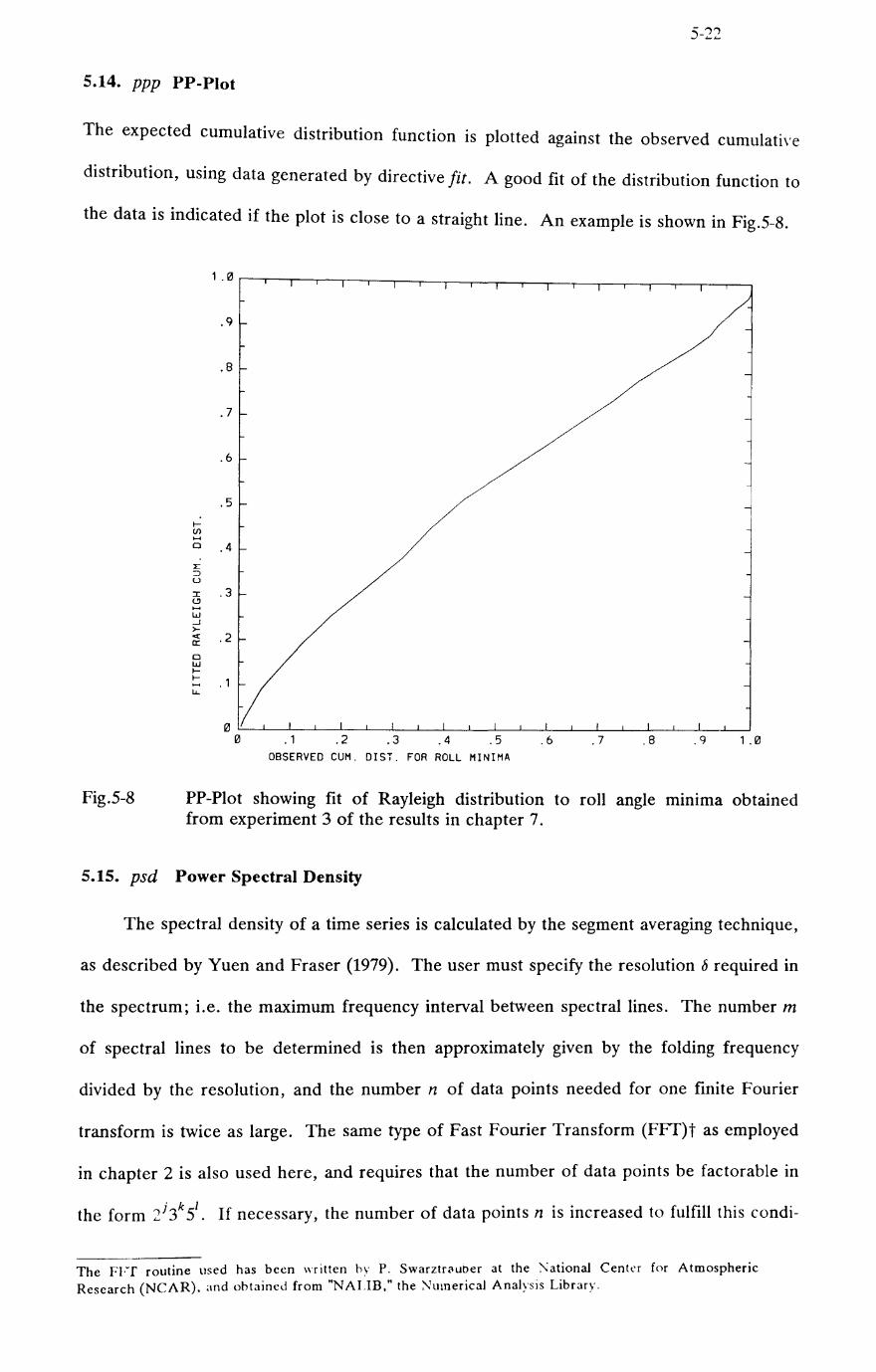
5.14. ppp PP-Plot
The expected cumulative distribution function is plotted against the observed cumulative
distribution, using data generated by directive fit. A good fit of the distribution function to
the data is indicated if the plot is close to a straight line. An example is shown in Fig.5-B.
Fig.5-B
1 .0
.9
.8
.7
.6
.5
t-V> ..... a .4 :E ::;) U
::I: .3 (..!) ..... W ...J >-cc .2 a: 0 w t-t- .1 ..... lL.
OBSERVED CUM. DIST. FOR ROLL MINIMA
PP-Plot showing fit of Rayleigh distribution to roll angle mImma obtained from experiment 3 of the results in chapter 7.
5.15. psd Power Spectral Density
The spectral density of a time series is calculated by the segment averaging technique,
as described by Yuen and Fraser (1979). The user must specify the resolution {) required in
the spectrum; i.e. the maximum frequency interval between spectral lines. The number m
of spectral lines to be determined is then approximately given by the folding frequency
divided by the resolution, and the number n of data points needed for one finite Fourier
transform is twice as large. The same type of Fast Fourier Transform (FFf)t as employed
in chapter 2 is also used here, and requires that the number of data points be factorable in
the form 2i 3k 51. If necessary, the number of data points n is increased to fulfill this condi-
The FFf routine lIsed has been written hy P. Swarztr(luoer at the :\ational Center for Atmospheric Research (NCAR). and ohtained from "NAUB." the :\'umerical Analysis Library.

5-23
tion, which may also lead to a slightly smaller resolution. The time series is divided into a
number of segments p of this length. The FFT routine is used to calculate a set of Fourier
coefficients C jk' j=0,1,2, ... , m-1 for each segment k=0,1,2, ... ,p-1 , corresponding
to the Fourier coefficients in the hrm directive. A periodogram is obtained from the
squared magnitude of the Fourier coefficients for one segment. The periodogram is
smoothed with a Tukey window to provide the basic spectral estimates.
1 S'k =-
J ~
0.5, C jk ,2 +0.5, C(j+l)k ,2,
0.25 ic(j_l)k ,2 +0.5ic jk ,2 +0.25 ic(j+l)k ,2,
0.5ic(j_l)k ,2+0.5icjk ,2,
j=o
j=1,2, ... ,m-2
j=m-1
The final spectral estimates are obtained by averaging across the segments
k=p-l
1 Sj = - ~ Sjk'
P kdJ
j =0,1,2, . . . , m -1
(5.27)
(5.28)
An estimate of the standard deviation of the basic spectral estimates is also obtainable by
this approach, and given by
j=0,1,2, ... ,m-1, p>l (5.29)
Yuen and Fraser (1979) show that the standard deviations of the spectral lines of a
periodogram are approximately equal to their mean values, for Gaussian signals. Tukey
smoothing provides some reduction in the variability of the spectral estimates, and segment
averaging can provide high accuracy when a long enough signal is available, so that many
segments can be used. Applying the sampling theory of mean values (cf. the discussion
under the sin directive), the coefficient of variation of the spectral estimates is given by
U j v· ::::::
J s/'vl; , j=0,1,2, ... ,m-1, S·>o J (5.30)
This coefficient of variation may be plotted together with the spectrum. Examples of spec-
tra obtained with the psd directive are shown in Fig.7-19 to Fig.7-26.
Spectral moments Ak are calculated from
j=m-l
A k = ~ (j 8) k S r 5 jdJ
(5.31)
Inaccuracies in the higher order moments, due to errors in the high frequency tail of the

~-2-+
estimated spectrum, may be reduced by truncating this summation at a suitable frequency.
The following signal statistics are estimated from the spectral moments:
standard deviation = ~
mean period = >"0/>"1
zero-up-crossing-period = V>"0/>"2
crest period = V>"2/>"4
spectral width = Vr-1-->";:<-/-(>"-0->"4-)
5.16. stn Stationarity Check Along a Sample Record
(5.33)
(5.34)
(5.35)
(5.36)
This directive is introduced with a brief discussion of the concepts of stationarity and
ergodicity in an experimental context. Consider a real stochastic process (e.g. ship rolling)
denoted by x (t , j), where t represents time (defined over the real line), and j may be con-
sidered to be an index variable, taking integer values from the range (1,00) t. If the index
variable j is held fixed, and the time variable t is varied over its range, then one realisation
of the stochastic process is obtained. A roll time history, obtained from one experiment
might be considered to be part of such a realisation, but not a complete realisation, since it
would only extend over finite time. A set of such realisations for varying j is usually
referred to as an ensemble of realisations. If the time variable is held fixed at t l' then the
sequence of values of X(tl,j) for j=1,2, ... ,n, may be considered sample values of a ran-
dom variable. In the present context, it may be useful to exemplify the index variable (j)
by the various roll time histories that would have been obtained, if one experiment could
be repeated under "similar" conditions. Statistics of a stochastic process are, in general,
defined across the ensemble of realisations with time held constant. Hence, the statistics
are, in general, functions of time. For example, the mean value x(t) might be expressed by
j=n
1 x(t) = lim - L: x(t,j) (5.37)
n->oo n j=1
Similarly, the autocorrelation R (t 1 ,t 2) would be a function of two times
j=n
(5.38) n->oo n ;=1
If the mean value of a stochastic process is invariant with time, and its autocorrelation
t Although a countabk inde'\ set is indicated here. an uncountable set would be more precise, corresponding to the sd of all possible initial (:unditions.

5-=.5
depends only on the time difference (t 2-t 1)' then the process is said to be weakly station
ary, or stationary in the wide sense. Stationarity of higher order requires corresponding
results for higher order cross products than the autocorrelation. The statistics of a Gaus
sian process are uniquely determined by its mean and its autocorrelation function, hence
weak stationarity implies strict stationarity for Gaussian processes.
Since each experiment carried out only provides one realisation of the stochastic pro
cess underlying that experiment, it is not practicable to determine statistics across an
ensemble of realisations. Instead, temporal averages along that time series are calculated.
This implies an assumption of ergodicity; viz. that the process is stationary and that expec
tations across the ensemble of realisations are equal to the corresponding temporal aver
ages taken along the single realisation. Price and Bishop (1974), or Papoulis (1965) provide
further details concerning the concepts of stationarity and ergodicity.
If stationarity is required, then it is desirable to control experimental conditions to
ensure that stationarity is obtained. This is not always possible, for instance in ship trials
at sea, where the waves are provided by nature. If analysis of the results is to be based on
stationarity, then it may be advisable to check that stationarity prevails. Lacking an
ensemble of realisations, the stationarity check cannot be constructed directly from the
definition. Instead, some representative statistics of the process are estimated as temporal
averages, and the variation of these statistics during the experiment is examined. The fol
lowing procedure is applied:
(a) A time series from one experiment is split into a number of segments, each of suffi
cient duration to allow sensible estimates to be made of the test statistics. Sequence
numbers j=1,2, ... ,m are assigned to each segment in order.
(b) A number of sample statistics Y j are calculated for each segment J. These sample
statistics may include the mean, standard deviation, skewness, kurtosis, 5th and 6th
central moments, mean period, zero-up-crossing period, crest period, and spectral
width. The spectral statistics are calculated from a periodogram obtained by a FFf
of each segment (cL directive psd).
(c) The correlation coefficient r is calculated for each sample statistic and the sequence

number
j=m
1 -. -J .y L: J"Yj m j=1
r = ------------------
-U·U
I Y
5-26
(5.39)
where j ,yare estimated mean values, and U j ,uy are standard deviations of the seg-
ment index and sample statistic respectively.
(d) The probability FR(r) that the sample correlation coefficient will not be exceeded, is
calculated applying Student's distribution with (m-2) degrees of freedom and argu
ment 7 defined by
(5.40)
This test is based on the procedure suggested in section 31.19 of Kendall and Stuart (1979).
It provides a test for the hypothesis that the calculated values of the test statistic are ran-
dom samples from the same underlying distribution, against the alternative of linear trend.
This ,test is distribution-free, in the sense that no ,specific form of distribution function is
assumed to underly the test statistic. However, the exact permutation distribution function
of the sample correlation coefficient is approximated using Student's distribution. This
approximation is obtained by fitting moments, and is exact up to the third moment, with an
error term of order m -1 in the fourth moment. Hence, the resulting probabilities will have
reduced accuracy for a small number of segments m.
For a chosen significance level Q', the hypothesis of randomness is accepted provided
(5.41)
and rejected otherwise, where F R (r) is the probability that the value r of the sample corre-
lation coefficient will not be exceeded. Hence, at a 10% significance level, the time series
will be accepted as being stationary if F R(r) lies between 0.05 and 0.95 for all the test
statistics considered. This choice of significance level also implies that there is a 10% pro-
bability of wrongly rejecting the hypothesis of stationarity.
If the test indicates that a time series is not stationarY. then the magnitude of the
trend in the test statistic should be examined. Accepting linear trend to be present, the
trend range in the sample statistic y between the first and last segments of the time series
is gin'Il by

5-27
(5.42)
The amount of trend may possibly be sufficiently small as to be considered insignificant.
However, this judgement requires considerable insight. The directive provides plots of the
sample statistics against time, which include the estimated trend lines. Examples are
shown in Fig.7-8 to Fig.7-16.
If the hypothesis of stationarity is accepted, then the stn directive provides additional
results for estimated standard errors in the mean values of the sample statistics for the
whole time series. The mean value of each sample statistic listed in step (b) above is given
by
j=m
1 Y = - ~Yj (5.43)
m j=l
and the standard deviation in the individual estimates Y j for a sample statistic is estimated
by
j=m
1 u y = [ ~ (y j _j)2]1/2 (5.44)
m-l j=l
Assuming this standard deviation to be a reasonable estimate for the underlying value, then
the standard error in the mean value y of the sample statistic is
f. -;::;:, u IV;;; y y (5.45)
The standard error is, in effect, the standard deviation in the estimated value of a statistic.
This estimate of the standard error is based on classical results from the sampling theory
of mean values. This simple procedure to obtain the standard error is most useful for the
estimates of statistics whose theoretical sampling distributions are not available. The
number of segments m into which the time series is divided affects the estimates of the
standard errors. Increasing the number of segments tends to reduce the estimate of the
standard error until the condition of sufficient duration, from step (a) above, is violated.
5.17. tnd Detrending
Detrending is accomplished llsmg a procedure described by Otnes and Enochsen (1978).
Given a time series Xj ,j=-n/2, ... ,n(2, a polynomial is first fitted to the data by the
method of least squares, and then subtracted from the input time series to provide the
detrendcd output time series. For numerical efficiency, the number of data points

5-28
included n' =n +1 is forced to be odd, and the polynomial is given an origin at the mid
point of the time series. The detrending polynomial is written
j=-n/2, ... ,n/2, 0<m<4 - - (5.46)
where dk are the coefficients of the polynomial, and m is the order of the polynomial. To
solve for the coefficients, the following moments are required
P2 = ~ / = n(n2 -1)/12
~.4 (2 ) ') P 4 = LJ ] = n n -1 (3n ~ - 7) /240
P6 = ~ / = n(n2 -1)(3n
4-18n
2 +31)/1344
Ps = ~ / = n(n2-1)(5n
6-55n
4+239n 2-381)/11520
k=0,1,2,3,4
(5.47)
(5.48t)
(5.49)
(5.50)
(5.51)
where the summations are taken from j=-n/2 to j=n/2. The coefficients may then be
obtained in descending order, starting with the highest order coefficient required
(n 'q 4 -P4qo)(pi -n 'q 4)+(P2qo-n 'q2) (P4P2- n 'P6) d 4 = -------------------------------------
(PzP4- n 'P6)2 -(P; -n'ps)(pi -n'P4)
d 3 = (P2Q3-P4ql)/(PzP6-P;) , m>3
d 2 = [(P2Qo-n'Q2- d 4(PzP4- n 'P6)l!(pi -n'P4)' m>2
d 1 = (Ql-P4d3)/P2' m>l
do = (QO-dzP2-d4P4) In'
m=4 (5.52)
(5.53)
(5.54)
(5.55)
(5.56)
where n'=n+1 is the number of data points, and the coefficients are set to zero if they are
not required dk=O, k >m .
The detrending calculations are done in double precision, to reduce problems with
numerical error. For more convenient interpretation, the coefficients are transformed to a
polynomial with origin at the beginning of the time series, prior to output. An example of
results obtained with this directive is shown in Fig.7-18. Experience has shown linear
detrending to be effective, while a test with higher order detrending led to numerical errors
when the magnitude of the trend was large compared to the actual signal.
t There is a correction in equation (5.48) relative to Otoes and Fnochseo (1978).
6-1
6. Estimation of Roll Damping Coefficients
In order to apply the present theory to a variety of ships, it is necessary to have some
means of obtaining the relevant inertia, damping, and restoring coefficients of the equation
of motion. Prediction of the exciting moment has already been discussed in section 2.2
and in appendix B. The hydrostatic restoring coefficient C is traditionally expressed III
terms of the transverse metacentric height OM and the ship's displacement volume v
C = pg\lOM (6.1)
where p is the water density, and g is the acceleration due to gravity. A derivation may be
found in Newman (1977). If the ship's natural frequency Wn may be determined from
experiment, either on the ship or a model, then knowledge of the restoring coefficient may
be used to obtain the inertia coefficient A
2 - 2 A = C /wn = pg\lGM /wn (6.2)
Failing this, it is necessary to estimate the dry inertia coefficient 14 from the ship's mass
distribution and obtain the hydrodynamic added-mass coefficient A44 by means of potential
theory. For instance, the close-fit technique formulated by Frank (1967) may be applied.
Such an approach can also be utilised to provide sway and sway-roll added mass coeffi-
cients, thus allowing a roll axis to be determined to minimise the coupling with sway (d.
section 1.4 and appendix B). Having disposed of the other coefficients of the equation of
motion, we may now proceed with the damping coefficients, as the main topic of this
chapter.
Two alternative damping functions f3(j) are considered
f32(j) = DJ; +D~ Ij I f33(j) = BJ; +B-J3
(6.3)
(6.4)
referred to as linear plus quadratic damping, and linear plus cubic damping, respectively.
The linear plus quadratic form of damping has been widely applied since Froude's paper of
1872, while the linear plus cubic form is less commonly used, but convenient for applica-
tion in the theory involving Volterra functionals. Dalzell (1978) has discussed both forms
of damping function, and found both models fitted a few sets of roll decay data reasonably
well.
6-2
Let us consider the basis for the choice of these two damping models. Transfer func
tions for roll response, obtained from model tests (cf. Fig.l-l), show that the roll response
is highly resonant in nature, implying that the damping is relatively small. Linear potential
theory calculations, assuming a non-viscous fluid, lead to damping coefficients correspond
ing to the energy in radiated waves. Intuitively, or through experiment, we may observe
that the other ship motions tend to dissipate more energy through radiated waves than the
roll motion does. In fact, a circular cylinder, oscillating about an axis in the still water
plane, would not radiate waves; i.e. would have zero roll damping in terms of potential
theory. It thus seems likely that other damping mechanisms, not present in linear potential
theory, may have to be included. The physical mechanisms that are usually considered in
addition to radiation damping are: (a) skin friction, (b) eddy-making, and (c) lift effects on
appendages due to forward speed. Himeno (1981) and Schmitke (1978) discuss roll damp
ing components in these terms. Sometimes the terms "viscous damping" and "eddy
making damping" are used interchangeably, but this usage is imprecise since skin friction is
also an effect of viscosity.
(a) Skin friction is due to the tangential stress between the ship hull and the sur
rounding water. Myrhaug and Sand (1980) have made a theoretical study of skin friction
damping for both laminar and turbulent boundary layers, considering only 2-dimensional
flow. The roll damping effect of skin friction was found to be linear for laminar flow con
dItions, which tend to be obtained in model tests. In turbulent flow, the damping moment
due to skin friction was found to be slightly nonlinear, and a relatively smaller part of the
total damping than in laminar flow. Since turbulent flow tends to be the case at full scale,
this indicates that some correction to the skin friction component of roll damping may be
necessary when scaling up from model test results.
(b) Eddies or vortices are induced when the boundary layer flow separates from the
hull surface. This effect leads to a change in the pressure distribution over the hull sur
face, producing a moment about the roll axis, part of which is in phase with the roll velo
city and acts as a damping moment. Separation is most readily induced by a sharp edge
such as a bilge keel, but may well occur in the absence of any such edge, if the necessary
flo\\' conditions arise. It appears to be common practice to assume that the eddy-making

6-3
component of roll damping is quadratic (cf. Schmitke 1978). The theoretical basis for this
assumption is not clear, but an analogy with the quadratic expression for the drag force
acting on a flat plate in a steady flow springs readily to mind, and seems likely to have had
some influence on this formulation. Himeno (1981) suggests that there is an element of
amplitude dependence in the component of the eddy-making damping, due to the pressure
forces acting directly on the bilge keel.
(c) Roll damping due to lift effects is discussed by Schmitke (1978). Appendages
may be considered to act as wings, protruding into the water flowing past the ship, generat
ing lift forces and the associated roll moments. This damping component is treated as a
linear function of the roll velocity, and as being proportional to the forward speed of the
ship.
Clearly, there is a strong basis for a linear roll damping component; from wave
making, from skin friction (a), and from lift effects (c). The theoretical basis for a qua
dratic roll damping component is not equally strong, but there is at least a traditional basis,
founded on observations of rolling and various forms of analysis of such observations. In
comparison, there is hardly any basis for a cubic roll damping component, except that the
linear plus cubic model can be made to fit the data about as well as the linear plus qua
dratic model does.
Numerical methods to predict eddy-making damping have been developed by Bear
man, Downie and Graham (1982), Patel and Brown (1981), Ikeda and Tanaka (1983), and
by Braathen and Faltinsen (1987). In general, these methods are only applicable when a
sharp edge is present on the ship hull, to define the location of the separation point. The
effect of the free surface is sometimes neglected in these calculations. Braathen and Fal
tinsen have found that inclusion of a free surface in the theoretical formulation, and the
ensuing radiated waves, sufficiently alters the flow pattern to have a noticeable effect on
the calculated damping moment. This finding has some bearing on another problem; viz.
roll dan1ping is usually estimated in the absence of incoming waves, but incoming waves
are present in the practical response problem, and may affect the damping terms. This
problem is briefly addressed in the discussion included in appendix D.
6-4
6.1. Estimation of Roll Damping Coefficients from Experiments
Methods to estimate roll damping coefficients from decay tests and forced rolling
tests are derived in appendix D. Damping coefficients may be obtained for both the damp
ing models given by equations (6.3) and (6.4). Estimators for the linear plus cubic damping
coefficients only, have also been presented by Mathisen and Price (1984) in a prior report.
A perturbation method is used to develop the estimators for decay tests, while harmonic
analysis and energy methods are used for the two types of forced rolling tests. The results
of the perturbation analysis lead to somewhat different estimators that those which are
most widely used (cf. Dalzell 1978), and which date back to Froude (1872). Froude's
method assumes that the decrement in roll amplitude between a pair of successive maxima
and minima may be related to the energy absorbed by damping with a constant amplitude,
equal to the mean magnitude of the two adjacent extrema. This assumption appears to be
valid in the case of linear damping, but slightly inaccurate in the case of nonlinear damp
ing, and it is avoided with the perturbation analysis. Some improvement in the estimated
damping coefficients may be expected on the basis of the relaxation of this assumption,
with the greatest effect when the roll decrements are relatively large. In addition, Froude's
method requires the use of the differences in amplitudes between pairs of adjacent
extrema, in the estimation process, while the perturbation estimators use the amplitudes of
the extrema directly. Such differences in amplitude are likely to be more affected by
experimental errors, particularly for small roll angles. Thus, there are some grounds for
expecting an improvement with the perturbation estimators, due to effects at both ends of
the decay process.
The estimators derived in appendix D have been applied by Spouge and Ireland
(1986), though little discussion of the results is given in that paper. Results from five dif
ferent methods of analysing decay tests have been compared by Spouge (1987), and good
results were reported with the perturbation estimators.
6.2. Results from Estimation of some Damping Coefficients
Dimensionless damping coefficients are presented. in order to case comparison
between the results for different ships. The linear damping coefficients arc presented in

6-5
terms of the critical damping for the response frequency; that is as D d(2A w), and as
B d(2A w). No equally obvious way of presenting the nonlinear damping coefficients is
available. To make them comparable to the linear coefficients, the expressions for the
energy dissipated in one cycle of harmonic rolling (given in section 4.2 of appendix D) are
divided by the energy which would be dissipated by critical damping. A roll amplitude
must be specified for this formulation, and 0.1 radians or 5.7 ° is chosen, as a convenient,
representative, small amplitude. Hence, the nonlinear damping ratios are presented as
D2 ·OA/(37rA) and B3· 0.03w /(8A). The quadratic damping ratio is proportional to the
chosen amplitude (0.1 radians), and the cubic damping ratio is proportional to the square
of this amplitude.
6.2.1. Damping coefficients for the FPV Sulisker
Nlodel tests with the FPV Sulisker were used to obtain the results given in the paper
in appendix D. Some additional results and figures are included here, that were omitted
from the paper for the sake of brevity. Refer to appendix D for details of the ship model
and the tests. Fig.6-1 and Fig.6-2 show data from two decay tests, together with the
corresponding sequence of roll angles given by the estimated damping coefficients for the
two damping models. The data from decay test 3A in Fig.6-1 may be seen to be of some
what poorer quality than the data from test 3B in Fig.6-2, since many adjacent pairs of
extrema have about the same value. This may be due to an inaccuracy in the calibration of
the mean (upright) position, or in manually reading off the amplitudes. A little additional
difficulty was encountered in locating the coefficient values which provided the minimum
residual sum of squared deviations for the poorer data. This required some variation of
the initial estimates of the coefficients in the minimisation procedure. The results of the
three decay tests are reproduced as percentages of critical damping in Table 6-1. Observe
that approximately the same sum is obtained from the two terms in either model, about
3.5% of critical damping. If the roll amplitude is doubled to 11..+°, then the total damping
increases to about 5.5%.
Results of a forced rolling test are shown in Fig.6-3 and estimated damping coelfi
dents arc given in Table 6-2. A slightly better agreement between the observed data and

Fig.6-1
Fig.6-2
6-6
.40r-'-~'-il-'~-'--'-~~~-'-'II--r-r-'-~~~~~ L:INEAR+ U8 C
-o c( a::
W -.J t!)
z c(
-.J -.J 0 a::
.35
.30
.25
.20
.15
.10
.05
0 0 2 SE~UENCE
LINEAR+&UAD. OBSERVED
Xl
4 6 8 10 12 14 16 18 20 NUMBER OF EXTREMA
Roll decay test for FPV Sulisker model configuration series 3, test A .
-o c( a::
w
. 35
.30
.25
.20
.15
. 10
G .05 z c(
-.J -.J
22
~ 0 L--L __ L--L __ L--L __ L--L __ L--L __ L--L--L--L--L--L~~~~~~~2'0 o 2 4 6 8 10 SE~UENCE NUMBER OF EXTREMA
Roll decay test for FPV Sulisker model configuration series 3, test B.

Table 6-1
Table 6-2
Fig.6-3
6-7
Series 1 Series 3A Series 3B Linear plus quadratic damping model
Dd(2Aw) 0.0128 0.0153 0.0163 D,·0.4/(37rA) 0.0215 0.0191 0.0198
Linear plus cubic damping model
Bd(2Aw) 0.0262 0.0270 0.0293 B,,·0.03w/(BA) 0.0069 0.0063 0.0059
Damping ratios estimated from decay tests with a model of the FPV Sulisker.
Series 1 Series 3 w=3.2 rad/s w-2.85 rad/s
Linear plus quadratic dam Ding model
Dt/(2Aw) 0.0115 0.0129 D?·0.4/(37rA) 0.0210 0.0198
Linear plus cubic damping model
Bt/(2Aw) 0.0331 0.0387 B ,,·0.03w/(8A) 0.00439 0.00351
Damping ratios estimated from forced rolling tests with a model of the FPV
Sulisker .
. 35
.30
.25
.20
.15
-0 c(
a:: - . 10
w 0 :::) ~ ...... -Q.
. 05 :I: c(
...J
...J 0 0:: 0
II
1 /
7 /
/ /
0 .5 1.0 , .5
(EXCITING MOMENT AMPLITUDE)
2.0 2.5
" SINE(PHASEI
3.0 3.5 4.0 4.5 5.0
(NMI
Forced rolling test for the FPV Sulisker model configuration series 3.
the linear plus quadratic model is discernible in Fig.6-3, than for the linear plus cubic
model. Better agreement between the damping coefficients estimated from the decay tests
in Table 6-1 and the coefficients estimated from the forced rolling tests in Table 6-2 is also
6-8
evident for the linear plus quadratic model. Additional points in favour of the linear plus
quadratic damping model are mentioned in appendix D; viz. a smaller residual sum of
squared deviations between fitted model and observed data, and a tendency to constant
values for the estimated coefficients irrespective of the roll amplitude.
Damping coefficients estimated from forced rolling tests are shown as a function of
frequency in Fig.6-4, for the linear plus quadratic damping model. As the frequency devi-
ates from the resonance frequency, wn =3.22 rad/s, the phase angle between the exciting
moment and the roll response approaches 0° or 180°. Since the energy absorbed by the
damping is proportional to the sine of the phase angle (cf. equation 42 of appendix D), the
accuracy of the estimated coefficients is critically dependent on the accuracy of the phase
angles. These angles are difficult to determine accurately far from resonance, hence the
ragged tendency shown by the results in Fig.6-4. The negative linear damping coefficient at
a frequency of 3.0 rad/s is assumed to be due to this type of inaccuracy. Any definite
trend with frequency is concealed by the uncertainties present in these results. However,
Fig.6-4 is based on a set of preliminary data, and it is possible that additional experimental
work might provide an improvement in the results.
6.2.2. Damping Coefficients for a Containership
Principal parameters of a model of a containership are given in Table 6-3. A series
of decay tests, forced roll tests, and regular wave tests with this model, have been carried
out and described by Blok (1985). During the tests, the model was held in position in the
tank with an arrangement of soft springs. The springs were also used to tow the model for
tests with forward speed. There was some concern that this spring arrangement might
affect the results, but variation of the spring rates and the location of the connections to
the model did not reveal any significant influence on the results. The rudder was inactive
during the tests. A magnetic tape of the test results was obtained and data from the decay
tests were analysed for inclusion here. The original analysis of the decay tests had been
carried out with Froude's method.
The level crossing algorithm of the time series analysis program, described in chapter
;;;; ,< S used to extract the maxima and minima of each decay record from the data in time _ , \\ .1.

Fig.6-4
Table 6-3
6-9
1 ." -I'll .. - -.. -0 .8 ¢ 0::
" If) -x: z - .6
lSI ~
" I'll 0 .4
-0 ¢ a: .2 " If) x: z -
0 0
If) I-z
-.2 UJ ..... U ..... u.. u.. w 0 u -.4 (,!J z ..... Q. x: cc 0 -.6
2.0 3.0 3.2 3.4 3.6 3.8 4.0 4.2 4.4 4.6 4.8 5.0 FRE~UENCY (RAO/S)
Variation of estimated linear plus quadratic damping coefficients with frequency, from forced rolling tests with a model of the FPV Sulisker.
length / beam beam / draught block coefficient transverse metacentric height / beam roll gyradius / beam, in water bilge keel span / beam bilge keel length / ship length model scale
Principal parameters of the containership model.
6.5 4.3 0.52 0.092 0.37 0.016 0.30
1:40
series form. Inspection of plots of the decay records showed some inaccuracy in the zero,
and 7 of the 26 record were corrected for this effect. Damping coefficients were estimated
for each test, using the estimators described in appendix D. The first extremum was omit-
ted from the estimation process in all cases. The results are shown in Fig.6-5 and Fig.6-6.,
with the damping ratios plotted against the Froude number. Fig.6-5 shows the linear damp-
ing ratios, while Fig.6-6 shows the quadratic and cubic damping ratios. Results were
obtained both with and without bilge keels (indicated by B.K. on the figures). The bilge
keels provide a consistent increase in the damping coefficients. Many of the tests were
repeated three times, and the separate values are shown as individual symbols in the fig-
ures. Satisfactor~' a~rcemcnt is indicated he tween the repeated tests. A marked increase
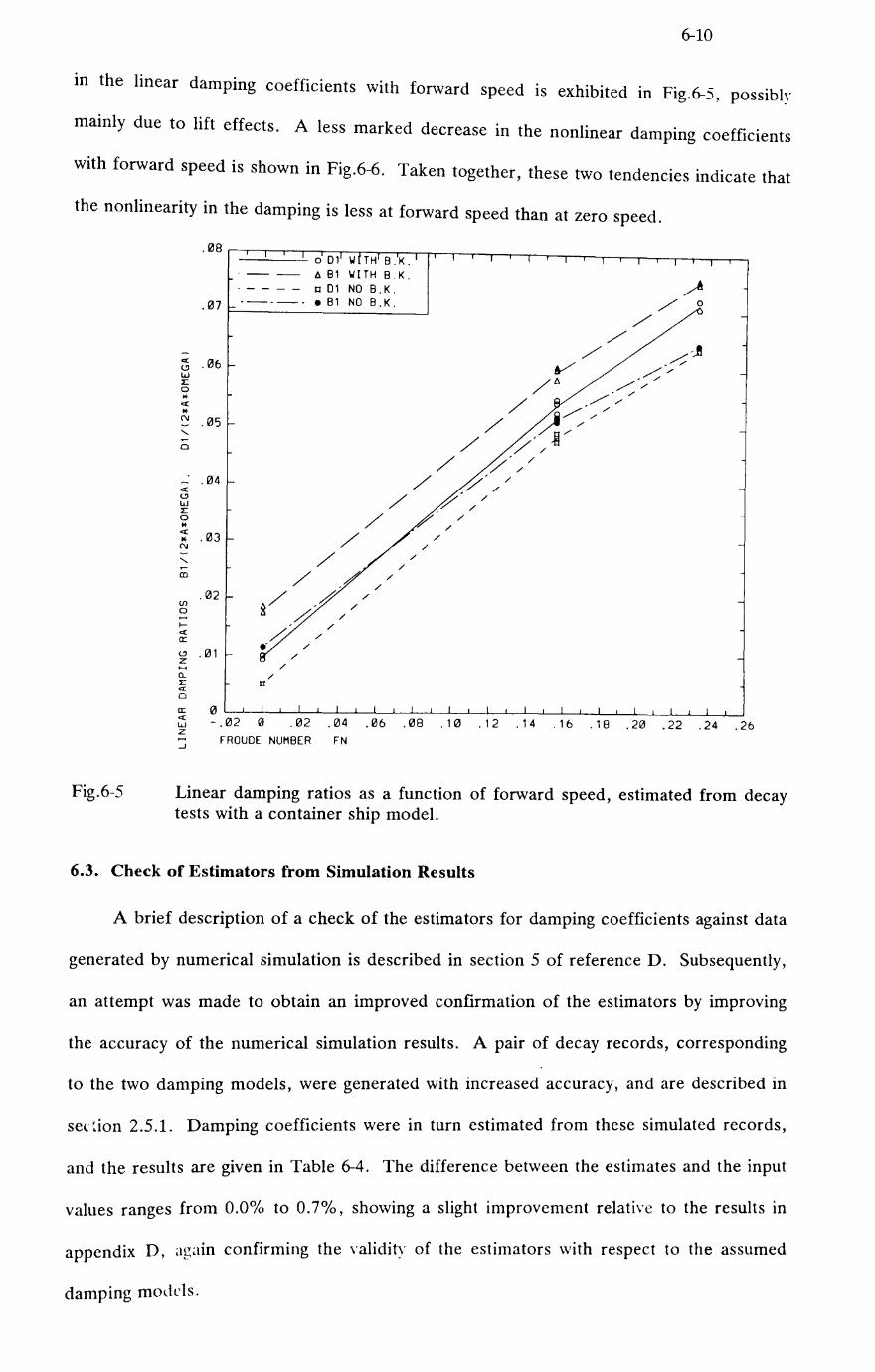
6-10
III the linear damping coefficients with forward speed IS exhibited in Fig.6-5, possibly
mainly due to lift effects. A less marked decrease in the nonlinear damping coefficients
with forward speed is shown in Fig.6-6. Taken together, these two tendencies indicate that
the nonlinearity in the damping is less at forward speed than at zero speed .
Fig.6-S
. 08'2~~~iIW~~~TT"~-r'-~~~,-~~~,-~~ 1---"':"001 --- t:.B1
II 01
.07r-·==_·==_· __ ·_B_l ________ ~
;3 .06 w ::E o .. ~ .. N .05 "-
- .04 ~ <.!) W ::E o .. :: .03 N -"-CD
If)
o ...... I~ ~
.02
<.!) .01 z ..... a.. ::E ~ o
/ II
/ /
~ 0 ~~~L-~~~~~~~~~~~~~~~~~~~~~~~~ ~ - . 02 . 16 . 18 .20 .22 .24 .26 z ~ FROUOE NUMBER FN
Linear damping ratios as a function of forward speed, estimated from decay tests with a container ship model.
6.3. Check of Estimators from Simulation Results
A brief description of a check of the estimators for damping coefficients against data
generated by numerical simulation is described in section S of reference D. Subsequently,
an attempt was made to obtain an improved confirmation of the estimators by improving
the accuracy of the numerical simulation results. A pair of decay records, corresponding
to the two damping models, were generated with increased accuracy, and are described in
sel~ion 2.S.1. Damping coefficients were in turn estimated from these simulated records,
and the results are given in Table 6-4. The difference between the estimates and the input
values ranges from 0.0% to 0.7%, showing a slight improvement relative to the results in
appendix D, again confirming the validity of the estimators with respect to the assumed
damping models.

Fig.6-6
Table 6-4
-ex: .. .....
. 018
'; .016 M
cs:. .014 .. C\I o
; .012 .. CD
...... ~ .01(2) w r o * M cs:. .008 cs:. .. M (l)
(f)
o ..... ~ ex:
.006
0: .004
..... a. ~ .002 o
0: ex: w z ..... ..J Z o z
o
0_
~ -.:::: ===--= -
o
-=--
6-11
. K. - - t; B3 '.I[TH B.K . - - - - c 02 NO B. K .
. -.-.• B3 NO B.K
o o
- --- - :::-- __ t; -- ---- --~ ----- T---.. a-- -..
.--------_. _._----.-.-. D
-------. .08.10.12.14.16.18.20.22.24.26
FRQUOE NUMBER FN
Nonlinear damping ratios as a function of forward speed, estimated from decay tests with a container ship model.
Simulation Estimates
input same model alternate model Linear plus quadratic damping model
Dl Nms/rad 0.5120 0.5109 Bl 0.8248 D? Nm(s/rad)2 3.430 3.442 B-" 5.811
Linear plus cubic damQ.ing model
Bl Nms/rad 1.470 1.470 Dl 1.250 B't Nm(slrad)3 2.540 2.557 D, 1.844
Comparison of damping coefficients used as input to numerical simulation with results estimated from the output.
The input data for the two damping models were equivalent, to some extent, since
both sets of damping coefficients were obtained from the same set of forced rolling tests.
Hence, it seemed possible that fairly similar decay records would be produced by simula-
tion of both decay models, and that estimated damping coefficients would not be strongly
dependent on which damping model had been simulated. The results for the alternate
models in Table 6-4 show that this is not the case; e.g. coefficients for the linear plus cubic
model estimated from simulation with the linear plus quadratic model differ strongly from
the estimates originally obtained from the forcf:d rolling model test.

7-1
7. Results of Analysis of Experimental Data for Ship Rolling in Irregular Waves
7.1. The Irregular Wave Tests
The tests were carried out by NMI Ltd., using the same model of the FPV Sulisker, as
described in Appendix D, but with a slightly different loading condition, specified in Table
7-1. The present loading condition has considerable trim, while there was no trim in the
mechanically forced rolling tests, cf. Spouge and Ireland (1986).
Model Scale Full Scale Draught amidships m 0.230 4.60 Trim, aft m 0.14 2.8 Displacement t 0.1915 1532 Transverse metacentric height, GM m 0.0390 0.78 Measured natural roll period s 1.96 8.77
Table 7-1 Loading condition for model of FPV Sulisker during irregular wave tests. The model scale is 1:20.
The model had twin rudders, but no other appendages. Roll and pitch were measured by a
gyro located near the model centre of gravity, while surface elevations were measured with
2 resistance-type wave gauges fore and aft of the model. The accuracies of the transducers
were stated to be approximately % 0 for the gyro and 0.05 inch for the wave probes at
model scale (0.025 m full scale). Surge, sway and heave were measured using light lines
attached to the model, and passing around pulleys attached to rotary potentiometers on the
towing tank carriage. Only roll motion and wave elevation data from tests in irregular,
long-crested, beam waves are considered here. The tests were carried out in the No.3 tow-
ing tank of NMI Ltd at Feltham, which is 400 m long, 14.6 m wide and 7.6 m deep, and
has an electro-hydraulic, plunger type wavemaker. The model was positioned about 100m
from the wavemaker and prevented from drifting along the tank by light lines attached to
the bow and stern, near the waterline. These lines passed over pulleys on the tank walls
and were held in tension by weights, as shown in Fig.7-1.
Data from experiments with four different sea states were provided on digital mag-
netic tape, digitised at 16 Hz model scale, corresponding to 3.58 Hz full scale. The test
results had already been scaled up to full scale, and this scaling was retained in the subse-
quent analysis. Since experiments 1 to 3 were rather lengthy, each signal was split into two
files on the magnetic tape. Prior to analysis. the data for each signal were read from the

7-2
~RAVEL
Fig.7-1 Arrangement to restrain model from drifting.
tape, the two files rejoined, and the data entered in the database of the time series analysis
program described in chapter 5. The long duration of the experiments, up to 3% hours full
scale, is unusual, and particularly valuable for the present investigation of the response
statistics of a nonlinear system. It also implies that the total amount of data is quite large;
viz. 423,360 data values, or 51/2 million characters. Roberts and Dacunha (1985) have also
utilised data from a different subset of the same model tests, and state that it was neces
sary to generate the data for each experiment from two runs in the tank, in order to avoid
excessive distortion of the wave motion due to reflection from the tank ends and walls.
7.2. Visualisation of the Data
Having entered the data in the database, some plots of the time traces were made, to
gain familiarity with the data, and to check for any anomalies. Fig.7-2 to Fig.7-4 show sam
ple plots of the three signals for experiment 3. These time traces are fairly typical of all 4
experiments. Good agreement is generally shown between the two wave probes in Fig.7-2
and Fig.7-3, although individual wave crests and troughs may be seen to differ in magni
tude. The surface elevation is defined as positive in a wave trough. The roll signal in
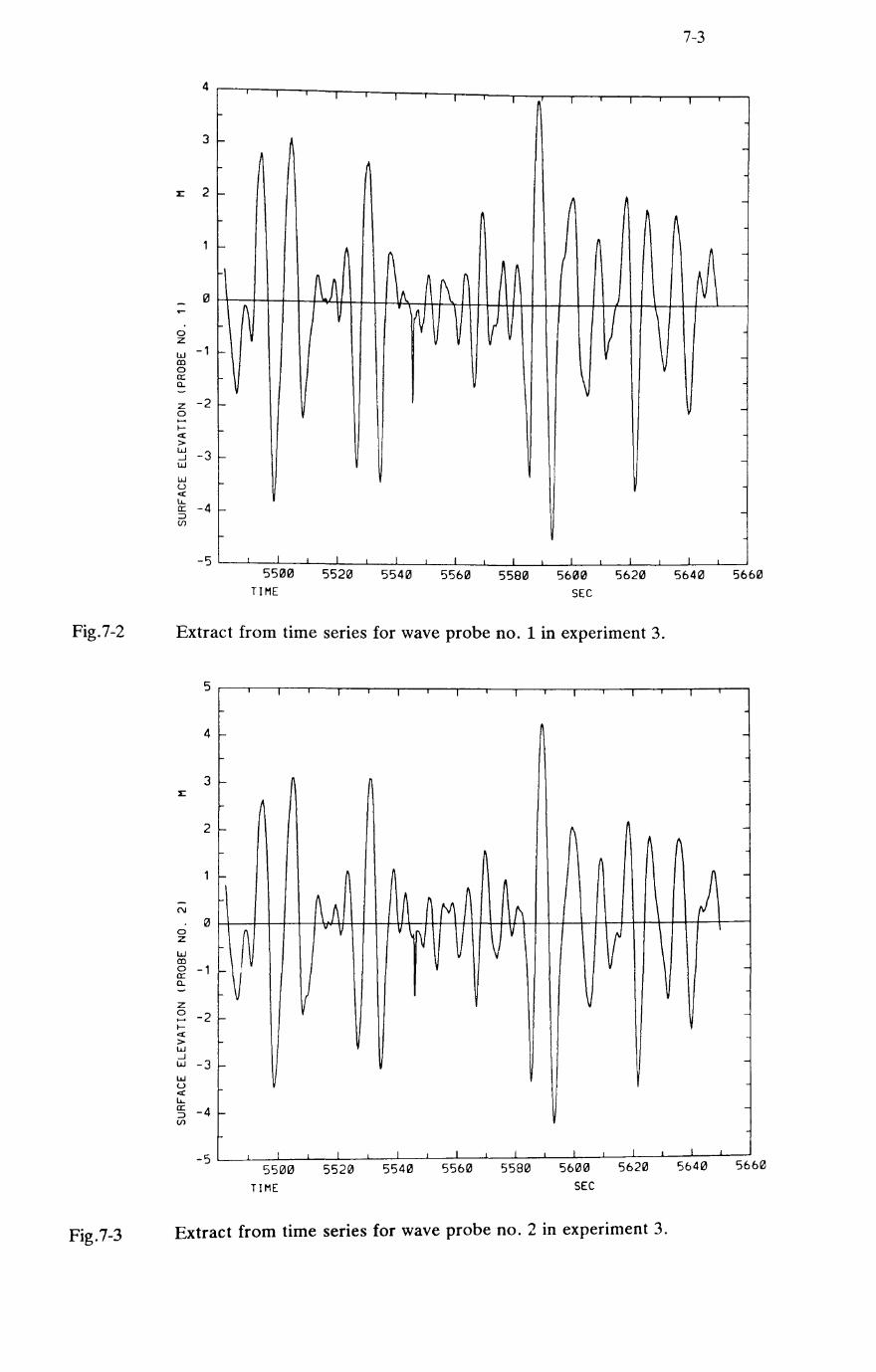
Fig.7-2
Fig.7-3
4
3
0
0 z w -1 m 0 a:: Q. -z -2 0 ...... I-ex: > w -3 -.J w W u ex: La..
-4 a:: :::l (f)
-5
I-
-
I-
>-
v I-
-
-
I
A
I
5500 TIME
I
~p
I
5520
I I T
A \/\ ~f\
~ \
V
I I I
5540 55613 55813
I
~
~
I
5600 SEC
I
/ \ v
I
5620
Extract from time series for wave probe no. 1 in experiment 3.
5
4 I-
3 I-
2 -
--N
0 0 z w m 0 -1 a:: -Q. -Z 0 -2 I-I-ex: > w -.J w -3 I-w u ex: La.. a:: :::l -4 I-(f)
-5
I
"
A
I
5500 TIME
V
I
AA v V
I
55213
I I
~ n ~
M v
N V V
I I
55413 55613
,-
fI V
I
55813
,-
~
V
I
56130 SEC
,-
h
V
I
56213
Extract from time series for wave probe no. 2 in experiment 3.
7-3
I
-
h
A -
N\
-
-
-
I
5640 56M'J
I
-
-
-fI
} -
-
-
-
-
I
5640 5660

Fig.7-4
30
25 -(J) w w 20 c:: -<..!l w a
15 -
10 -
5
0 -0 :1
-5 I-
-10 I-
-15 l-
w --1 <..!l z -20 ex: ---1 --1 0 -25 c:: -
-30
~
I
ft
I
5500 TIME
I I
V V
I I
5520 5540
I I
An J V VV
V
I I
5560 5580
I
V
I
5600 SEC
Extract from time series for roll angle in experiment 3.
7-.+
T I ~ -< -< ~
-j
-
-
~ -
A -
-
-V
-
-
-
I I
5620 5640 5660
Fig.7-4 exhibits a somewhat less irregular nature than the wave signals, indicative of it's
more narrow-banded spectrum. The two files comprising each of the signals are joined
together in the middle of these time traces, at 5566 s on the time axis. There is no visible
sign of a discontinuity at this point on any of the three time traces included here, or at the
corresponding points on the time traces from experiments 1 and 2 (not shown). Thus, the
joining together of the signal pieces should not have any significant effect on the subse-
quent analysis. However, a sharp spike is apparent at 5546 s along the time axis on all 3
time traces. This spike appears to be too narrow to represent the true wave and roll
motion, and is very likely the result of some electrical disturbance in the signal processing.
A little roughness may also be discernible on some of the peaks and troughs of the signals,
possibly indicative of some high frequency noise in the signals. Hence, it appears
wo. thwhile to low-pass filter the signals, in order to reduce the effects of such spikes and
high frequency noise.
Fig.7-5 to Fig.7-7 show compressed time traces of the entire signals for experiment 3.
These compressed time traces confirm a fairly uniform behaviour of the signals throughout
the experiments. and show that there are no large amplitude drop-outs present. Some

Fig.7-5
Fig.7-6
0 z w m 0 a: Q. -z 0
I-c:r:: > w ....J W
w u c:r:: I.J... a: :::J (f)
4
3
2
0
-1
-2
-3
-4
-5
-6
-7 0
TIME
7-5
8000 9000 10001 11001 12000
SEC
Compressed time trace for wave probe no. 1 in experiment 3.
-N
o z w
4
3
2
o
-1
~ -2 a: a.
z -3 o .-.. Ic:r:: > -4 w ....J W
~ -5 c:r:: I.J... a: ~ -6
-7 L-~-L~ __ L-....l--L-....l __ L-~-L-....l __ L-....l--L~ __ L-~-L~--L-~-L~~ o 1000 2000 3000 4000 5000 6000 7000 8000 9000 10001 11001 12000
TIME SEC
Compressed time trace for wave probe no. 2 in experiment 3.

Ul 30 LrJ LrJ a: '-' LrJ o
LrJ ...J '-' Z c:c ...J ...J 0 a:
20
10
o
-10
-20
-30
-40 0
TIME
7-6
8000 9000 10001 11001 12000
SEC
Fig.7-7 Compressed time trace for roll angle in experiment 3.
asymmetry is clearly present in the wave signals in Fig.7-5 and Fig.7-6, with a tendency for
high waves to have greater peaks (negative values) than troughs. A corresponding ten-
dency for large roll oscillations to have greater positive than negative extrema may also be
discerned, though this tendency is not quite so obvious. Again, the compressed time
traces shown for experiment 3 are typical of the corresponding figures for the other experi-
ments (not shown).
7.3. Stationarity Check
A stationarity check was carried out on all the data, using the method described in
chapter 5. This appeared advisable, because the long duration of the experiments might
have lead to a gradual build-up of reflected waves in the tank. Each of the signals were
split into a number of segments for the stationarity check. The length of the segments was
chosen to be of about 1000 s duration, giving about 100 roll cycles in each segment. The
following statistics were calculated for each segment: mean, standard deviation, skewness.
kurtosis, mean period, zero-up-crossing period, crest period, and spectral width. Integra-
tion of the spectra was truncated above 0.4 Hz in the calculation of the periods and spec-
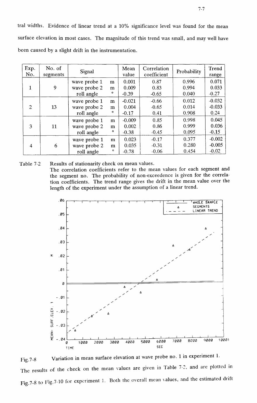
7-7
tral widths. Evidence of linear trend at a 10% significance level was found for the mean
surface elevation in most cases. The magnitude of this trend was small, and may well have
been caused by a slight drift in the instrumentation.
Exp. No.
1
2
3
4
Table 7-2
Fig.7-8
No. of Signal
Mean Correlation Trend segments value coefficient
Probability range
wave probe 1 m 0.001 0.87 0.996 0.071 9 wave probe 2 m 0.009 0.83 0.994 0.033
roll angle 0 -0.39 -0.65 0.040 --0.27
wave probe 1 m -0.021 --0.66 0.012 --0.032 13 wave probe 2 m 0.004 -0.65 0.014 --0.033
roll angle 0 -0.17 0.41 0.908 0.24
wave probe 1 m -0.009 0.85 0.998 0.045 11 wave probe 2 m 0.002 0.86 0.999 0.036
roll angle 0 -0.38 -0.45 0.095 --0.15 .-wave probe 1 m 0.023 -0.17 0.377 --0.002
6 wave probe 2 m 0.035 -0.31 0.280 --0.005 roll angle 0 --0.78 -0.06 0.454 -0.02
Results of stationarity check on mean values. The correlation coefficients refer to the mean values for each segment and the segment no. The probability of non-exceedence is given for the correlation coefficients. The trend range gives the drift in the mean value over the length of the experiment under the assumption of a linear trend .
. 06
.05
.04
.03
:I: .02
.01
0
- .01
> ~ - .02 w
I..&... 0:
~ - .03 I
Z < W :I: -.04
r-
r-
r-
r-
'-
-
-
r- '" '" '" 6.
o TIME
I I r I I I I WHoLE SAMPLE 6. SEGMENTS
. - - -- LINEAR TREND
6. -
,/ ,/
,/ -,/
6. / ,/
~ ,/
,/ -/
,/
/ ,/
/ -/
,/
,/
,/ 6.
,/ , ,
6. ,/
,/
,/ 6. ,/ -
'" ,/
,/
,/
,/
'" -
/ 6. ",tJ
'" ,/ -
I I I I I I I I I
1000 2000 3000 4000 5000 6000 7000 8000 9000 10001 SEC
Variation in mean surface elevation at wave probe no. 1 in experiment I.
The results of the check on the mean values are given in Table 7-2. and are plotted In
Fig.7-8 to Fig.7-10 for experiment I. Both the O\'erall mean values, and the estimated drift

Fig.7-9
Fig.7-10
·040
.035
.030
.025
L .020
.12115
.12110
.01215 N
> ~ 121 w I.J... a: ~ -.1211215
I Z <t: W L -.1211121
f-
-
'-
c-
c-
c-
-
-/ /6
o TIHE
I I
/ /
/
/ /6 /
/
I I
101210 21210121
I I I
/
6 / , /
/ 6 /
/ /
/ /
/ /
6
I I I 301210 41211210 512100
/
T
/ /
"t::.
I
61211210 SEC
6
. - - --
6
/ /
/ /
/ /
I 71211210
7-8
II/HoLE SAMPlE SEGMENTS LINEAR TRENO
-6
/ -/
/ /
/ / -
-6
-
-
-
I I
Variation in mean surface elevation at wave probe no. 2 in experiment 1.
VI w w a: <.!l w a
<.!l Z
.1215
121
-.1215
- . 1121
-.15
-.2121
-.25
-.3121
-.35
-.4121
..: -.45 ....J ....J o a: -.50
I z <
c-
I-
I-
I-
I-
I-.....
I-
-
-
-
-
~ - .55 o
A
.....
TIHE
I I I I T
..... ..... ..... ..... A ..........
..... ..... ..... ..... ..... ..... ..... ..... ..... ......
A ..... .....
A
A
I I I I I
1121121121 2121121121 312100 41211210 5121121121
Variation in mean roll angle in experiment 1.
I
..... A
.....
I 61211210 SEC
IWHoLE SAMPlE A SEGMENTS
0 ____ LINEAR TREND -
-
-
-
-
-
-
-
A
..... ..... 6-.... -
..... ..... ..... ..... ..... ..... A -..... ..... .... I I I
71211210 81211210 90121121 11211211211

Fig.7-11
Fig.7-12
1 .58
1 .56
1 .54
1 .52
1 .50
x: 1 .48
1 .46
1 .44
> Ij 1.42 w lL.
§ 1 .40 (J)
I Z o 1.38
.... ~ 1.36 Cl
Cl t-(J) 1. 34
""
-A
I-
I-
I-
-, ,
-
-
-
I-
-
o TIME
7-9
I I I I I I T WHoLE SAP1PlE A SEGMENTS
- - -- LINEAR TREND _
-
-
-
-
A -, , , , -, , , , , -, , , , , -, , , ,
A , 'lz..... ,
A , A , , -, A ,
I I I A I I I I '~ I
1000 2000 3000 4000 5000 6000 7000 8000 9000 10001
SEC
Variation in standard deviation from wave probe 1 in experiment 1.
11 .6 I I I I I I wHoLE SAMPlE
A SEGMENTS
11 .4 . - - -- LINEAR TREND
l-
11 .2 I- A -f1
(J) 11 .0 "" -w w a: <.!) w 0 10.8 "" -
A
10.6 - ~--
- --- - --- --u - --- -- -10.4 -- -- - --
<.!) Z
4: 10.2 ...J ...J o a:
.h 10.0 o .... t-4: .... > w o o t
9.8
(J) 9.6
-
l-
-
o TIME
A A -
t;,.
-t;,.
I I I I I I I I I
1000 2000 3000 4000 5000 6000 7000 8000 9000 10001
SEC
Variation in standard deviation of roll angle in experiment 1.
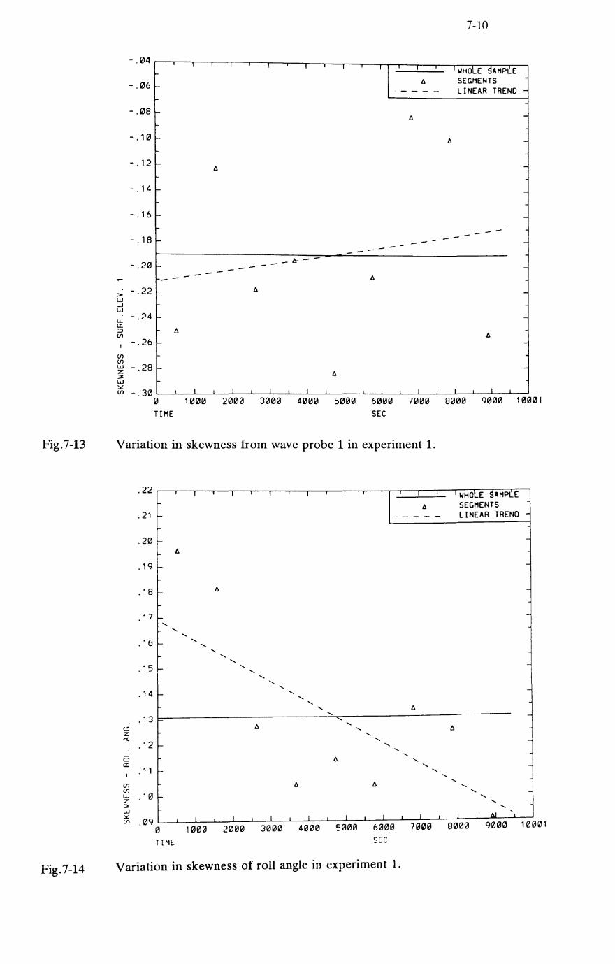
Fig.7-13
Fig.7-14
-.04
-.06
-.08
-.111l
-.12
- . 14
-.16
- .18
-.211l
> - .22 w -1 W l.L. - .24 0: ::> VJ
VJ VJ
-.26
~ - .28 ;:J: w :.:: VJ -. 311l
f-
-
-
-
r-
I-
f-
-- -
-
-A
-
-
\ \ \ \
A
- - - - - _Ir-
- - - -A
I I I I
7-10
T I WHoLE gAI'1PtE A SEGMENTS
- - - -- LINEAR TREND -
A -
tJ. -
-
-
-
- -- -- - - - - -- - - - - -
-
A
-
-
A
-A
I I I I I
III 201110 3000 4000 5000 60011l 7000 8000 9000 10001
TIME SEC
Variation in skewness from wave probe 1 in experiment 1 .
t!l z q:
-1 -1 0 0:
VJ VJ
. 22
.21
. 2 III
.19
.18
.17
.16
.15
.14
.13
.12
. 11
~ . 1 III ;:J: w ::.::
l-
f-A
I-
f-
f-'-
'-'-
f-
f-
-
-
-
-
-
\ \ \
tJ.
'-'-
'-'-
'-'-
'-'-
'-
tJ.
I I I
I I I
tJ. . - - --
'-'-
'-'-
'- A '-
"- ..... '-
'- ..... '-
'- ..... A .....
'-'-
tJ. tJ.
I I I I
\ WHoLE gAI'1PtE SEGMENTS LINEAR TREND
-
-
-
-
-
-
-
-tJ.
-
-.....
'-'-
'- -'-
'-'- ,
I 1\\
VJ .09 o 1000 2000 3000 4000 5011l1ll 6000 7000 8000 901110 10001
TIME SEC
Variation in skewness of roll angle in experiment 1.

Fig.7-15
Fig.7-16
2.0
1 .8
1 .6
1 .4
1 .2
1 . 13
.8
> .6 \.oJ ...J \.oJ
u... § .4 Ul
Ul ..... Ul o .... a: :::> ~
. 2
13
I-
.... A
-
f-
I-...... .....
I-
-
-
-
13 TIME
I I I
...... ...... "-
"-"- ...... .....
"-"- .....
"-
A
A
I I I
1131313 2131313 3131313
I
A
..... "- ...... .....
I
4131313
I
A ..... "-
I
5131313
......
T
...... A
.....
I
6131313 SEC
7-11
I wHoLE SAMPLE A SEGMENTS
0 ____
LINEAR TREND
-
-
-
-
-
-
A
-...... .....
...... ...... ......
"t. ..... -..... ...... ...... Il .........
I I I
7131313 8131313 11313131
Variation in kurtosis from wave probe 1 in experiment 1.
. 1
13
- . 1
-.2
-.3
-.4
<.!l
~ -.5 ...J ...J o a:
Ul -.6 ..... Ul o .... a:
A
-
..... ..... -
-
-
-
f-
~ - 7 • 13
TIME
I I I I 1 I I WHoLE SAMPLE A SEGMENTS
. - - -- LINEAR TREND
-A
Il
..... A -"- ...... "- ..... ..... ..... ..... ..... ..... ..... ..... -..... .....
Il u ...... -, ...... ..... ......
"- ..... ..... --.. ..... ..... ..... ..... ..... ..... ..... Il .....
Il -
I I , I I I I I Il,
1131313 2131313 3131313 4131313 5131313 6131313 7131313 80013 qQJQJQJ 11313131
SEC
Variation in kurtosis of roll angle in experiment 1.
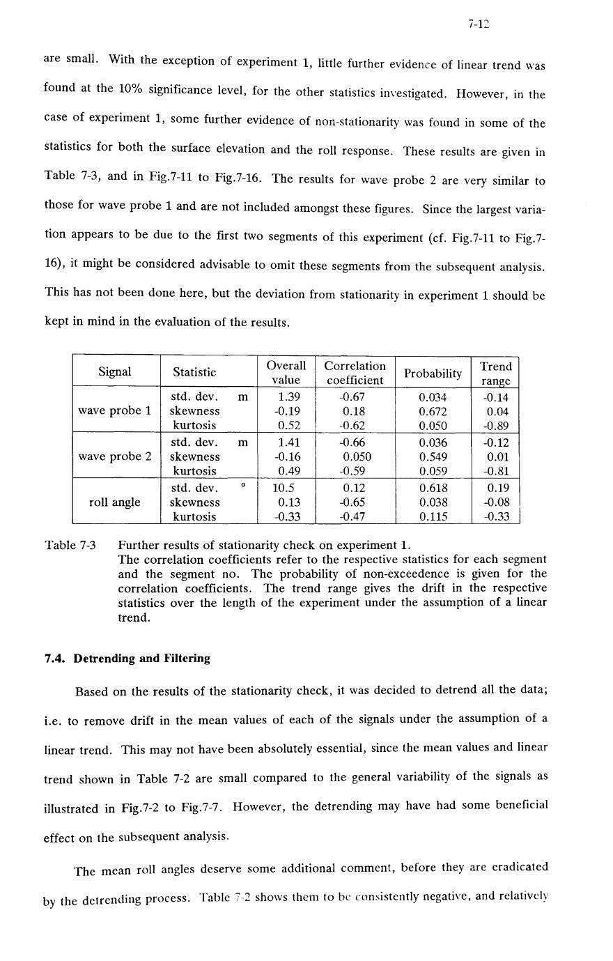
7-12
are small. With the exception of experiment 1, little further evidence of linear trend was
found at the 10% significance level, for the other statistics investigated. However, in the
case of experiment 1, some further evidence of non-stationarity was found in some of the
statistics for both the surface elevation and the roll response. These results are given in
Table 7-3, and in Fig.7-11 to Fig.7-16. The results for wave probe 2 are very similar to
those for wave probe 1 and are not included amongst these figures. Since the largest varia
tion appears to be due to the first two segments of this experiment (d. Fig.7-11 to Fig.7-
16), it might be considered advisable to omit these segments from the subsequent analysis.
This has not been done here, but the deviation from stationarity in experiment 1 should be
kept in mind in the evaluation of the results.
Signal Statistic Overall Correlation Probability
Trend value coefficient range
std. dev. m 1.39 -0.67 0.034 -0.14 wave probe 1 skewness -0.19 0.18 0.672 0.04
kurtosis 0.52 -0.62 0.050 -0.89 std. dev. m 1.41 -0.66 0.036 -0.12
wave probe 2 skewness -0.16 0.050 0.549 0.01 kurtosis 0.49 -0.59 0.059 -0.81 std. dev. 0 10.5 0.12 0.618 0.19
roll angle skewness 0.13 -0.65 0.038 -0.08
I kurtosis -0.33 -0.47 0.115 -0.33
Table 7-3 Further results of stationarity check on experiment 1. The correlation coefficients refer to the respective statistics for each segment and the segment no. The probability of non-exceedence is given for the correlation coefficients. The trend range gives the drift in the respective statistics over the length of the experiment under the assumption of a linear trend.
7.4. Detrending and Filtering
Based on the results of the stationarity check, it was decided to detrend all the data;
I.e. to remove drift in the mean values of each of the signals under the assumption of a
linear trend. This may not have been absolutely essential, since the mean values and linear
trend shown in Table 7-2 are small compared to the general variability of the signals as
illustrated in Fig.7-2 to Fig.7-7. However, the detrending may have had some beneficial
effect on the subsequent analysis.
The mean roll angles deserve some additional comment, before they are eradicated
by the detrending process. Table -;-2 shows them to be consistently negative, and relatively

7-13
larger than the mean surface elevations when compared to the corresponding trend ranges.
Taking the mean roll angles to be significant, though quite small, it seems worthwhile to
attempt an explanation as follows: The model restraining arrangement shown in Fig.7-1 is
intended to counteract the mean effect of wave drift forces. Assuming that the mean hor-
izontal drift forces have a line of attack below the mean waterline, while the restraining
force acts just above the waterline, then these mean forces will impose a couple on the
model, which will lead to a mean roll angle. Since the wave periods are relatively long, the
heave motion will tend to follow the waves fairly closely, thus tending to support the
assumption that the wave drift forces act below the mean waterline of the model. Unfor-
tunately, information on the positive sense of the roll angle is not available at the time of
writing, in order to check the consistency of this reasoning.
After detrending, the signals were low-pass filtered. The cut-off frequency of the
filter was set to 0.5 Hz, based on a preliminary spectral analysis of the data. The filter
characteristic is shown in Fig.7-17.
1.0~~--~1--~-'~~.---r-1-r--r-1-r--~1-'--'1--'--'1--'--'1--'--1_
.9 ~ \
a: o fU
.8 ~
.7 -
.6 f-
.5 ~
.4 .....
. 3 ~
.2 ~
.1 ~
~ 0 ~
FRE~UENCY HZ
Fig. 7 -17 Characteristic of low-pass filter applied to data signals.
-
-
-
-
-
A symmetric filter was used, which does not introduce any phase shift into the signals, but
d f h t· . A check on the mean values and 50 data points are lost at both en s 0 eac tme serIes.

7-14
standard deviations of the s· I b f d f . Igna s e ore an a ter the filtenng process showed that no sig-
nificant changes were introduced into these statistics. Fig.7-18 shows part of the same time
trace as shown in Fig.7-4, including the spurious spike. Both raw and filtered signals are
plotted in the figure, confirming that the filtering process has partially smoothed out the
spike without leading to any undesirable distortion of the signals. The effect of detrending
may also be discernible at the maxima and minima of the signal.
Fig.7-18
(f)
w w a: t!l w 0
w .-J t!l z c:(
.-J
.-J 0 a:
30
25
20
15
10
5
-5
-10
-15
-20
TIME
--
5520 5525 5530 5535 5540 5545 5550 5555 5560 5565 5570 SEC
Extract from time series for roll angle in experiment 3, showing both raw data and detrended and filtered signal.
7.5. Wal'e and Roll Spectra
Spectra have been calculated from all three filtered signals for the four experiments. The
spectra are shown in Fig.7-19 to Fig.7-26. The wave spectra from the two wave probes are
plotted on one figure, followed by a separate figure with the roll spectrum for each experi-
ment. A resolution of 0.003 Hz was specified for these spectra, allowing the average of
from 39 to 15 periodograms to be taken (dependent on the length of each experiment), and
leading to a coefficient of variation between 0.08 and 0.2 for the spectral densities. Zero-
up-crossing periods and spectral widths have been calculated from the spectra, and arc
given in Table 7-4. The integration was truncated at 0.4 lIz in the calculation of these

Fig.7-19
Fig.7-20
50
45 N I "-C\I M 40 M ::E
35
> 30 w ....J W
lJ... 25 0: ::;) (/)
>- 20 l-
(/)
Z W 0 15 ....J c(
0: I-U w 10 a. (/)
0: W 3 5 0 a.
0 0 .10 .15 .20 .25 .30
FRE~UENCY HZ
Wave spectra, for both wave probes, from experiment 1.
N I "-C\I .. .. (/) w W 0: l!l W 0
l!l Z c(
....J
3500
3000
2500
2000
is 1500 0:
>l-
(/)
~ 1000 o
....J c(
0: I-
~ 500 a. (/)
0: W
7 -1.5
.35
1 2
.40
3 o a. o ~±±~~LLLL~~~~~~~~~LL~~~~~LL~~~
o .05 . 10 . 15 .20 .25 .45
FREI:IUENCY HZ
Roll spectrum from experiment 1.

Fig.7-21
F· 7 ')') 19. -........
36
34
32 N :r: "- 30 N w w
28 ~
26
24
22 > w ...J 20 w lJ.. 18 a: :::> (f)
16
>-14 t-......
(f)
z 12 w 0
...J 10 ex: a: t-
B u w Cl. (f) 6 a: w
4 :l< 0 Cl.
2
0 0 .05 .10 .15 .20 .25 .30
FRE~UENCY HZ
Wave spectra, for both wave probes, from experiment 2.
5500
N ~ 5000 N w K Ul W W a: '-' w o
t!l Z «
4500
4000
3500
3000
...J 2500
...J o a:: >- 2000 t-
Ul
~ 1500 o ...J cC e: 1000 u w Cl. (f)
a:: w :l< o Cl.
500
FRE~UENCY
Roll spectrum from experiment 2.
HZ
7-16
.35
1 2
.40

Fig.7-23
Fig.7-24
30
28
N 26 I "-N M 24 M l:
22
213
> 18 w -.J W 16 --I.i.. a::: ::)
14 (J)
>- 12 f-....... (J)
z 113 w 0
-.J 8 c(
a::: l-Ll W 6 CL (J)
a::: 4 w ::x 0 CL 2
0 0 .135 .10 .15 .213 .25 .313
FRECilUENCY HZ
Wave spectra, for both wave probes, from experiment 3.
5000
45130
N I ...... N 413130 M .. (J)
w w a::: 35130 <..!)
w 0
30130
251313 <..!)
z c(
-.J 2131313 -.J 0 a::: >-f- 151313 (J)
z w 0
-.J 113130 c(
a::: f-u W 0.. 500 (J)
a::: w ::x 0 0.. 0
13 .135 .113 .15 FRECilUENCY
Roll spectrum from experiment 3.
.213 .25 HZ
7-17
.35
1 2
.413
.45

Fig.7-25
Fig.7-2()
55
5eJ N I "-N 45 M M x:
4eJ
35
> w -.J 3eJ w
I.J... ex: :::J (/)
25
>-l-
(/) 2eJ z w 0
-.J 15 c(
ex: I-u w a. 1 eJ (/)
ex: w ~ 0 5 a.
eJ 0 .05 .10 .15 .20 .25 .30
FREQUENCY HZ
Wave spectra, for both wave probes, from experiment 4.
350eJ N I "-N .. M (/) 3eJeJeJ w w ex: t!l w 0
250eJ
201ZleJ
-.J
6 1500 ex:
>l-
(/)
~ 1 eJ0eJ o
-.J c(
ex: I-
~ 5eJeJ a. (/)
ex: w ::E o a.
FRE~UENCY
Roll spectrum from experiment 4.
HZ
7-18
.35
1 2
,40
1

7-19
spectral parameters. Good agreement is shown between the wave spectra derived from the
two wave probes. The roll spectra may be seen to be narrower than the wave spectra in all
4 experiments, and to peak near the natural frequency of 0.114 Hz. Although the signifi-
cant wave height is least in experiment 2 (ct. Table 7-5), comparison of the wave spectra
shows this experiment to have the greatest wave energy in the region of the roll natural fre-
quency, and to give the largest roll standard deviation (ct. Table 7-6). There is some low-
frequency content in the roll spectra, which appears to be greater than the roll response to
be expected from the corresponding low-frequency content of the wave spectra. This low-
frequency roll motion might possibly be due to the same sort of mechanism as suggested
for the mean roll angles above; i.e. a roll moment being produced by the restraining lines
in conjunction with the slowly varying horizontal wave drift forces, and now complicated
by the dynamics of the slow drift sway motion.
Exp. No. of Zero-up-crossing period [s] Spectral width
periodo- wave wave roll
wave wave roll no.
zrams probe-1 probe-2 probe-1 probe-2 1 28 8.95 8.96 8.84 0.64 0.64 0.43 2 39 7.40 7.48 8.46 0.57 0.57 0.37 3 33 8.18 8.24 8.72 0.65 0.64 0.38 4 15 8.90 8.96 8.85 0.67 0.66 0.43
Table 7-4 Results derived from spectral analysis.
7.6. Distribution of Continuous Signals
Normal and Edgeworth distributions have been fitted to the continuous signals for the
roll angle, and from the wave probes. The parameters of the fitted distribution functions
are given in Table 7-5 and Table 7-6. Since the signals have been detrended, the mean
values are zero in all cases. Standard errors have been estimated for the distribution
parameters, and are included in Table 7-5 and Table 7-6t. In general, the values of skew
ness and kurtosis are large compared to the standard errors, confirming that these statistics
are significant. The kurtosis obtained for the surface elevation in experiment -+ forms an
exception in that it has a negative sign, while it is positive for the other 3 experiments.
This result should not be taken as significant, since it's standard error is relatively large.
t U h b made of the stationarity check to obtain the standard errors. There is some difference in se as een . . . .. d Th'
al S "crl'ved from the stationarity analysis and in the dlstnbutlOn flttmg proce ure. IS the parameter v ue u . k . f . I I ean \alues and standard deviations are used to estImate the skewness and urtosls or arises because oca m
Exp.
No.
1 2 3 4
1 2 3 4
Table 7-5
Table 7-6
7-20
No. of Wave probe - 1 Wave probe - 2
data std.dev. skewness std.dev.
fml kurtosis fm]
skewness kurtosis
33980 1.40 -0.19 0.59 1.41 -0.16 0.54 47900 1.18 -0.25 0.31 1.19 -0.22 0.26 39744 1.27 -0.15 0.08 1.28 -0.13 0.07 19100 1.54 -0.21 -0.10 1.55 -0.18 0.13
Standard errors - 0.022 0.024 0.141 0.020 0.024 0.134 - 0.011 0.013 0.082 0.011 0.010 0.071 - 0.019 0.018 0.051 0.020 0.014 0.051 - 0.032 0.034 0.095 0.031 0.031 0.089
Distribution parameters for continuous signals from wave probes. The second half of the table gives the standard errors in the estimates of the corresponding parameters.
Exp. No. of Roll angle
No. data std.dev. fOl skewness kurtosis 1 33980 10.5 0.13 -0.31 2 47900 11.8 0.19 -0.49 3 39744 10.8 0.16 -0.33 4 19100 11.3 0.11 -0.62
Standard errors
1 - 0.15 0.012 0.067 2 - 0.12 0.010 0.054 3 - 0.28 0.009 0.039 4 - 0.17 0.009 0.038
Distribution parameters for continuous roll signal. The second half of the table gives the standard errors in the estimates of the corresponding parameters.
Values of skewness and kurtosis different from zero indicate that the underlying sto-
chastic process is not a Gaussian process. Since this analysis aims, in part, to check
theoretical results derived from an assumption of a Gaussian excitation process, it is unfor-
tunate that this assumption should not be adhered to in the available model test data.
However, the skewness of the wave elevation may well reflect a tendency to higher peaks
and flatter troughs that is often claimed for ocean waves. Bitner-Gregersen (1983) gives
some results for skewness and kurtosis obtained from analysis of wave buoy measurements
in the northern North Sea, at a water depth of 144m. These statistics are estimated from
records of only 17 minutes duration and must suffer from considerable random error.
Selecting the 20 cases given with significant wave height between 4 m and 6 m, there are 13
each segment in the one case, while overall mean values and standard deviations are used in the other case.
The difference was considered insignificant for the present data.

7-21
negative and 7 positive values of skewness in the range (-0.164, 0.069). The positive sense
of the skewness in the reference is not given. There are 8 negative and 12 positive values
of kurtosis in the range (-0.367, 0.626). Hence, this data gives some confirmation that the
values of skewness and kurtosis obtained for the waves in the model tests are not
unrepresentative of ocean waves.
If a stationary stochastic process is Gaussian, then an ordinary scalar spectrum pro
vides an adequate frequency-domain description of the process. Higher order spectra are
required to describe non-Gaussian processes. Such higher order spectra provide a descrip
tion of relationships between different frequency components in the process. This descrip
tion is superfluous for a Gaussian process, since it's frequency components are indepen
dent. In the frequency domain, the skewness in the wave signal may be interpreted as the
result of some preferential phase relationship between peak frequency and high frequency
components in the waves, by analogy with a Stoke's wave. The tuning of the present
experiments would provide a resonant roll response to the peak frequency component, but
little response to the high frequency component, thus attenuating the skewness in the
response. However, the skewness of waves and roll response is of much the same magni
tude in the present tests. It is possible that an explanation of the skewness in the roll
response may be found through the interaction of a different set of frequency components;
viz. the resonant and low frequency components of the roll response. In the discussion of
the roll spectrum, it was suggested that the low-frequency components might arise through
the joint effects of the wave drift force and the model restraining system. During the pas
sage of a large wave the wave drift force tends to increase, and this could produce an
increase in the roll moment in conjunction with the restraining system. The unidirectional
nature of such a nonlinear effect would explain a skewness in the roll response.
The positive kurtosis of the surface elevation indicates a preponderance of large
elevations as compared to a Gaussian process, while the negative kurtosis of the roll signal
indicates an opposite effect. Intuitively, it seems unreasonable that the positive kurtosis in
the excitation process should lead to the opposite effect in the response. The same sort of
frequency response reasoning as applied to the skewness would also seem to lead to an
attenuation of the kurtosis. HO\\'C\'er, the negative kurtosis in the roll response can be

7-22
explained very well by nonlinear damping. In fact the magnitude of the kurtosis obtained
from the model tests in Table 7-6 compares favourably with the results by numerical simu
lation in Table 2.6.
Normal and 2nd order Edgeworth distributions have been fitted to the surface eleva
tion and roll signals, using the fit directive of the time series analysis program. Observed
and fitted distribution functions are plotted in Fig.7-27 to Fig.7-31. Most of these figures
refer to experiment 3, which was selected because the surface elevation signal showed the
smallest deviation from the normal distribution, in terms of skewness and kurtosis. Fig.7-
27 and Fig. 7-28 show probability density functions and cumulative distribution functions for
the surface elevation. Close agreement between the observed data and the fitted distribu
tion functions is exhibited in Fig.7-27. The long negative tail gives an indication of some
skewness. The cumulative distribution function in Fig.7-28 is plotted on normal probability
paper, which provides straight lines for Gaussian distributions. This form of plot
highlights the deviations in the tails of the distribution. A tendency is apparent in the data
for large negative values (peaks) to occur more frequently, and for large positive values
(troughs) to occur less frequently than predicted by the fitted Gaussian distribution. This
tendency is followed somewhat better by the Edgeworth distribution. Fig.7-29 and Fig.7-30
show the corresponding density functions and cumulative distributions for the continuous
roll response in experiment 3. The observed probability density lies below the normal den
sity, both in the negative tail, and at the mean value, while agreeing closely in the positive
tail in Fig.7-29. The reduced probability of large negative roll angles relative to the normal
distribution is brought out more clearly in the cumulative distribution in Fig.7-30, and some
tendency for reduced probability of large positive roll angles may also be indicated. Again,
the 2nd order Edgeworth distribution follows the observed distribution more closely than
the normal distribution does. Although experiment 4 was the shortest in duration, it did
produce the smallest roll skewness and largest roll kurtosis of the set of experiments. As a
result, this experiment most clearly exhibits a tendency to reduced probability of large roll
angles relative to the normal distribution, and the resulting cumulative distribution function
is also included in Fig.7-31.

Fig.7-27
>-f-
...J ....... CD ex: CD 0 a: Q.
w > f-ex: ...J ~ :r:: ~ u
Fig.7-28
.34
.32
.30
.28
.26
.24
.22
.20
.18
.16
.14
>- .12 ..... ..... (/) z .10 w 0
>-..... .08 ..... ....J .06 ..... (lJ ex: (lJ .04 0 a:: n.
.02
0 -7
SURFACE ELEVATION (PROBE NO. 1 I 11
7-23
NORMAL orST. EOGEW •• 2
5
Probability density functions for surface elevation at waveprobe-l ill experiment 3.
0.99990 OBSERVED
0.99950 --- NORMAL DIST. 0.99900 - - - -- EDGE'W. . 2
0.99500 0.99000
0.95000
0.90000
0.70000
0.50000
0.30000
0.10000
0.05000
0.01000 0.00500
0.00100 0.00050
0.00010
/ /
/ /
77 77
.../ V7 -10.00 -5.00
SURFACE ELEVATION (PROBE NO.1)
/ V
/
0.00
711
7
T /1
7 /
M
II: W 0.. .. 0..
>~
.= CD .. CD o II: 0..
..J .. r II: o Z
Cumulative distribution functions for surface elevation at waveprobe-l ill experiment 3.

Fig.7-29
>-~ ...... -l
m c::(
m 0 a: 0..
w > ~ c::(
-l ::> L ::> u
Fig.7-30
7-24
- - NORMAL DIST. - - - - EDGEW.. 2
.035
.030
.025
.020
.015 >-I-.... (f) z w 0
.010 >-I-.... ..J ..... Q)
« Q) .005 0 a:: Q.
~4~0~~~_~3L0~---L--L--i--J---L--L--~~--~~L--L~~~--J-~50
ROLL ANGLE DEGREES
Probability density functions for roll angle in experiment 3.
I OBSERVED NORMAL DIST. ---
0.gggg0
0.ggg50 0.ggg00 - - - -- EDGE'W. , 2
0.gg500 0.gg000
0.g5000
0.g0000
/ /
/ /
V
0.70000
0.50000
0.30000
0.10000
0.05000
/j //j
/1 / Tf
/
0.01000 0.00500
0.00100 0.00050
0.00010 -40.00 -20.00
ROLL ANGLE 0.00
)V /
/
20.00
7 7'
7 /
40.00 DEGREES
Cumulative distribution functions for roll angle in experiment 3.
a:: ... 0.. <C 0..
>... ..J
(D
'" CD a a:: 0..
..J
'" I: a:: a z
60.00

0.99990
0.99950 0.99900
0.99500 0.99000
0.95000
0.90000
0.70000
>- 0.50000 l-I-<
-.J 0.30000 I-<
CD e:(
CD 0 0.10000 0: Cl..
w 0.05000 > I-<
l-e:( 0.01000 -.J :::> 0.00500 :E :::> u 0.00100
0.00050
0.00010
OBSERVED --- NORMAL DIST. - - - -- EDGE"" .• 2
/ / /
/
'1 ~
// / / /
/j 1/ I
7-25
r: I
)// /'l
V /
/ /
V
/
<r w 0.. c: 0..
>>-
..J
m c: m o <r 0..
;;( J: <r o z
-40.00 -20.00
ROLL ANGLE 0.00 20.00 40.00
DEGREES
Fig.7-31 Cumulative distribution functions for roll angle in experiment 4.
x2 tests were applied to test the fit of the normal and 2nd order Edgeworth distribu-
tions to the observed continuous data. In most cases, this test led to a formal rejection of
the hypothesised distribution functions. However, this formal result should not be taken
seriously, because:
(a) The data values are not fully independent, and therefore do not fulfill one of the con-
ditions of the test.
(b) The test does not allow for the effects of random experimental error.
(c) The i test is very powerful when applied to such large amounts of data.
It is sometimes suggested that the first objection (a) can be avoided by reducing the sam-
pIing frequency, in order to reduce the correlation between adjacent data points. This .,
approach discards information about the random variable, reducing the power of the \. ~
test, and can easily lead to acceptance of a hypothesised distribution by disregard of a suf
ficient amount of evidence (d. also the discussion in chapter 5). Instead of using the /
test as a formal test of fit, the \: 2 statistic is used as an indicator of the amount of deviation
between the observed data and a fitted distribution, in the present context. Provided that
approximately the same number of degrees of freedom (DOF) are applied, small values of

7-26
Waveprobe-l Roll angle Exp. Normal Edgeworth Normal Edgeworth
2 DOF 2 2 2 no. X X DOF X DOF X DOF
1 747 83-85 187 91-95 498 109-111 241 95-99 2 879 113-115 186 117-121 1468 129-131 490 121-125 3 276 104-106 123 105-109 576 117-119 166 102-106 4 293 81-83 125 79-83 629 9395 196 84-88
Table 7-7 Results of X2 test for fit of continuous data to normal and 2nd order Edgeworth distributions.
the X2 statistic indicate a better fit than large values do. The results in Table 7-7 confirm a
closer fit to the data by the Edgeworth than by the normal distribution. This applies to
both the surface elevation and the roll angles. Except for experiment 1, the results also
indicate a greater deviation from the normal distribution by the roll angles than by the sur-
face elevations.
7.7. Distributions of Maxima and Minima
Maxima and minima of the surface elevation and roll signals have been found using
the level crossing directive of the time series analysis program. The sampling frequency of
3.58 Hz implies 31.4 samples per cycle at the roll natural frequency, and a maximum error
of 0.5% in the detected maxima and minima, under assumption of a sinusoidal peak shape
(cf. section 2.4.1). The greater width of the wave spectrum may well cause a slightly larger
error in peak and trough heights.
Rayleigh and constrained gamma distributions have been fitted to the maxima and
minima of both processes. The parameters of the fitted distributions are given in Table 7-8
to Table 7-11.
Table 7-8
Waveprobe-1 Waveprobe-2 Exp.
No. of Maxima Minima No. of Maxima Minima no. extrema T} rml 1] rml extrema 1] fml Tl rml 1 1016 1.85 2.13 1016 1.87 2.14 2 1755 1.53 1.82 1733 1.56 1.83 3 1323 1.67 1.91 1317 1.70 1.93 4 562 2.04 2.39 565 2.06 2.37
Parameters of Rayleigh distributions for maxima and minima of surface elevation.
Probability density functions and cumulative distribution functions for the observed data
and fitted distributions are shown in Fig.7-32 to Fig.7-39. Distributions of maxima and

7-27
Waveprobe-1 Waveprobe-2 Exp. slope f3 scale fr [m] slope f3 scale fr [m]
no. max. mm. max. mm. max. mIll. max. mIll. 1 1.69 1.40 1.62 1.50 1.68 1.44 1.62 1.58 2 1.96 1.44 1.51 1.34 1.93 1.53 1.52 1.44 3 1.91 1.59 1.61 1.57 1.77 1.65 1.54 1.64 4 2.70 1.75 2.41 2.15 2.65 1.74 2.41 2.11
Table 7-9 Parameters of constrained gamma distributions for maxima and minima of surface elevation.
Exp. No. of Maxima Minima Mean From std. dev. no. extrema 1] -l- [0] 1] rOl ( 1].!. +1] J /2 rOl (J V2 rOl 1 1064 15.0 14.6 14.8 14.8 2 1579 16.9 16.3 16.6 16.7 3 1275 15.5 15.0 15.3 15.3 4 592 16.2 15.8 16.0 16.0
Table 7-10 Parameters of Rayleigh distributions for roll angle maxima and minima.
Exp. Slope parameter f3 Scale parameter fr [0]
. . . . no. maxIma mmIma maxIma mIllIma
1 2.20 3.37 15.9 18.6 2 2.42 5.50 19.0 22.6 3 2.12 3.56 16.1 19.4 4 3.20 5.38 20.4 21.9
Table 7-11 Parameters of gamma distributions for roll angle maxima and minima.
mImma are shown separately, with corresponding density and distribution functions on
each page. The cumulative distribution functions are plotted on Weibull probability paper,
which provides a straight line for Rayleigh distributions, while gamma distributions may
produce curves in this format. (Note that the abscissa values of 5 on the Weibull paper
apply with the corresponding exponent of 10 shown to their left.) The figures shown apply
to experiment 3, but these results are reasonably representative of the 4 experiments.
The Rayleigh parameter for the distribution of maxima and minima of a narrow-
banded Gaussian process may be estimated from the standard deviation of the continuous
process as (J \.12. This estimate of the parameter is compared with the mean value of the
Rayleigh parameter estimated from the extrema themselves in Table 7-10. Surprisingly
good agreement is shown.
In Fig.7-:32, both fitted density functions follow each other closely. They also follow
the observed density of the \\avc troughs quite well, except for the smallest wave troughs.

7-28
This deviation is consistent throughout the experiments, and is related to the width of the
wave spectrum. The deviation for small wave troughs shows up more markedly in the
cumulative distribution in Fig.7-33. The slope parameter of the gamma distribution is 1.91
(d. Table 7-9),and fairly close to the value of 2.0 which coincides with the Rayleigh distri
bution. The distribution of the wave peaks in Fig.7-34 and Fig.7-35 may be seen to differ
somewhat from the wave troughs in the 2 previous figures, although the same deviation
between observed data and fitted distributions is apparent for small wave peaks. The slope
parameter of the fitted gamma distribution is now 1.59 (d. Table 7-9), and this is reflected
in a deviation with respect to the fitted Rayleigh distribution, which is apparent both
around the mode of the density function in Fig.7-34 and at the upper tail of the distribution
function in Fig.7-35. It appears that the gamma distribution follows the observed data
slightly better than the Rayleigh distribution does.
Since the roll spectrum is narrower, the observed probability density of small roll
angles approaches zero much more closely in Fig.7-36 and Fig.7-38, than for the wave
elevations. Otherwise, the distribution of roll maxima in Fig.7-36 and Fig.7-37 appears
much as the distribution of wave troughs in Fig.7-32 and Fig.7-33, though the gamma slope
parameter is now slightly greater than 2.0 at 2.12 (cf. Table 7-11). For the roll minima, the
gamma slope parameter is 3.56, and a corresponding reduction in the probability of large
roll minima is apparent in both the density function in Fig.7-38, and in the distribution
function in Fig.7-39. Comparing the magnitudes of the roll angles at a probability level of
0.99, Fig.7-37 shows about 33° for the maxima, while Fig.7-39 shows about 27° for the
minima from the gamma distribution and observed data, and 32° from the Rayleigh distri
bution.
x2 tests have also been applied to the fit of the Rayleigh and constrained gamma dis
tributions to the data for minima and maxima. The results of these tests are given in Table
7-12 and Table 7-13. In all cases, the i statistic indicates an improved fit with the gamma
distribution, although this improvement may not be significant for the wave elevation max
ima or for the roll maxima. However, the improvement is quite definite for the wave
elevation minima and the roll minima, and appears to be the largest for the roll angle
minima.

Fig.7-32
Fig.7-33
.60
.55 '--. - - - -
.50 / ~
.45 /
.40
.35
.30
.25
>-~ .20 .... / (fJ
z w 0
/ .15 >-~ ....
/ ...J .... .10 (l) co::
/ (l)
0 a: .05 Q.
0 0 .5 1 .0 1 .5 2.0 2.5 3.0 3.5
SURF.ELEV. 1 - MAXIMA M
Probability density functions for surface elevation maxIma (wave troughs) in experiment 3.
>-
0.99')')00
0.99')000
0.990000
0.900000
0.800000
0.700000 0.600000 0.500000
0.400000
0.300000
!: 0.200000 ....J >--< m e;(
~ 0.100000 0: 0..
W ;:: 0.050000 le;(
....J ::> L ::> u
---- - - --
/
OBSERVED RAYLEIGH OS GAMMA DrSTN.
L
V ~v I
L /
/.-V VI"
/ I
/v
L .
/ /
V rf
V
0.010000
1.0e-01 5 1 . 0e +00
SURF .ELEV. 1 MAXIMA
j /
L /
7-29
RAYLEIGH DST GAMMA DISTN,
4.0 4.5
at waveprobe-l
5 H
a: .., 0..
"" 0..
~ ~ -.J
m
"" m o a: 0..
.J
.J ~ m
Cumulative distributions for surface elevation maxIma at waveprobe-l (wa\'e' troughs) in experiment 3.

.50~' , , , r' , .
. 45'
.40
.35
.30
.25
.20 ~
// foo-..... (j) .15 z
/1 w 0
~
/1 foo-..... .H'J -l ..... CD
1 c(
CD 0 .05 a: a.
SURF.ELEV. 1 - MINIMA
\
\~ ~
\ ~ ~ ~
M
7-30
RAYLEIGH DST GAMMA DISTN .
Fig.7-34 Probability density functions for surface elevation m1ll1ma at waveprobe-l (wave peaks) in experiment 3.
Fig.7-35
>I-
0.999990 12l.999912l12l 12l.99912l012l
12l.990012l12l
12l.912l12l012l12l
I2l.BI2lI2lI2lI2lI2l 0.712l0012l12l 12l.612l0012l12l 0.512l00012l 0. 4000012l
12l.312l12l012l0
:; I2l .212l0012l0 ..... CD q: CD ~12l.112l0000 0...
w ~ 12l. 050000 Iq: -.J :::> 1: :::> u
I ---- - - --
V /'
12l.12l10000 1.0e-01
OBSERVED RAYLEIGH OS GAMMA DISTN.
// /~
:,,-
/ V ~ !/ 1/
V Lr/
/ / 1/
/' //
v "
5 1.0e+00
SURF.ELEV. MINIMA
f V
/ /
/
7 /1
Lr 7,
!/} t-r-' rJ
H
ex: ... Q. .. Q.
-...J II) .. II) o a: Q.
...J
...J ::> II)
.0e+01
Cumulative distributions for surface elevation mlmma at waveprobe-l (wave peaks) in experiment 3.

Fig.7-36
Fig.7-37
7-31
·060
.055 ._- RAYLE[GH OST . - - -- GAMMA O[STN .
.050
.045
.040
.035
.030
.025
>-I- .020 ...... Vl Z W 0
.015 >-I-...... ....J ..... .010 m ex: m 0 a:: .005 a..
0 0 10 15 20 25 30 35 40
ROLL ANG. - MAXIMA DEGREES
Probability density functions for roll angle maxima in experiment 3.
>-
0.999900
0.999000
0.990000
0.900000
0.800000
0.700000 0.600000 0.500000
0.400000
0.300000
: 0.200000 -l ..... CD ex: ~ 0.100000 a: a.. w ;:: 0.050000 fex: -l :::> l: :::> u
---- - - --
OBSERVED RAYLEIGH DSl GAHHA DISTN.
V l4
k4 fl
,,-
W/ j
/
I ~
V / I
/ /
/ ,1/
J/
-1
-I
45
II: ... IL C IL
...J
III C III o II: CI..
...J
; 0.010000
1.0e+00 '5 1.0e+01 '5
DEGREES 1.0e+02
ROLL ANG. MAXIMA
Cumulative distributions for roll angle maxima in experiment 3.

7-32
D . - - RAYLEIGH OST
- - - - GAMMA OISTN . . 07
.06
.05 I
/ I I
.04 / I
.03 I I >-f--...... (/) I I I z w 0
.02 It' >-f--...... -.J It' ...... CD <C CD .01 It' 0 cr: Cl.
I
0 0 5 10 15 20 25 30 35
ROLL ANG. - MINIMA DEGREES
Fig.7-38 Probability density functions for roll angle minima in experiment 3.
>-
0.999900
0.999000
0.990000
0.900000
0.800000
0.700000 0.600000 0.500000
0.400000
0.300000
:: 0.200000 -.l ..... CD e:(
~ 0.100000 ex: a.. w ;:: 0.050000 le:(
-.l :::> l: :::> u
---- - - - -
OBSERVED RAYLEIGH OS GAMMA DISTN.
/
V 'l / V / /
/ / / /
/ I /
I
I
~
f /
71 17
// ~
/ //
/J /j
j/ / /
/
I
40
a: ... 0.. .. 0..
>.... :; CD c: CD a a: 0..
...J
...J :;) CD
W ;]I
0.010000 1.0e+00 5 1.0e+01 5
DEGREES 1.0e+02
ROLL ANG. MINIMA
Fig.7-39 Cumulative distributions for roll angle minima in experiment 3.

Table 7-12
Table 7-13
Table 7-14
7-33
Maxima Minima Exp. Rayleigh Gamma Rayleigh Gamma
2 DOF 2
X2 2 no. X X nOF DOF nOF X 1 77 19-20 67 18-21 114 17-18 66 17-20 2 140 30-31 135 28-31 131 27-28 53 27-30 3 191 28-29 183 26-29 115 22-23 77 21-24 4 54 20-21 42 16-19 51 16-17 48 15-18
2 Results of ~ test for fit of maxima and minima from waveprobe-1 to Rayleigh and constramed gamma distributions.
~Aaxima Minima Exp. Rayleigh Gamma Rayleigh Gamma
no. X2 DOF 2 DOF X2 DOF 2
X X DOF 1 23 23-24 19 20-23 96 26-27 25 19-22 2 68 29-30 59 26-29 300 33-34 46 29-32 3 22 26-27 18 23-26 119 27-28 36 22-25 4 37 21-22 11 16-19 107 22-23 25 1720
Results of X2 test for fit of roll angle maxima and minima to Rayleigh and constrained gamma distributions.
Exp. Exp. Maxima Minima
frq. Obs. Bound Prob- Obs. Bound Prob-
no. frq. rOl ability frq. rOl ability
Rayleigh distribution
1 106 109 22.7 0.427 70 22.2 1.000 2 158 138 25.6 0.915 70 24.7 1.000 3 128 129 23.5 0.111 99 22.8 0.994 4 59 51 24.6 0.757 29 23.9 1.000
Gamma distribution
1 106 104 22.5 0.202 95 21.2 0.761 2 158 157 25.2 0.100 159 22.8 0.100 3 128 133 23.4 0.392 118 21.7 0.672 4 59 65 23.6 0.628 63 22.2 0.463
Results of tails test for fit of roll angle maxima and minima to Rayleigh and constrained gamma distributions.
The fit of the Rayleigh and constrained gamma distributions to the observed roll
angle maxima and minima has also been investigated by means of the tails test described in
chapter 5. The results of this test are given in Table 7-14. For each experiment, tail
regions of the probability distributions are defined by bounds at the value of roll angle
which is expected to be exceeded by 10% of the roll maxima or minima. The expected fre-
quency in the tail region is compared to the observed frequency, and the probability that
their difference will not be exceeded is computed. Little difference between expected and

7-34
observed frequencies is shown for the fit of both distribution functions to the roll angle
maxima. Large differences are shown for the roll angle minima, and the Rayleigh distribu
tion is rejected while the gamma distribution is accepted at a significance level of 10%.
In their analysis of data obtained from model tests with the FPV Sulisker, Roberts
and Dacunha (1985) averaged the histograms obtained for roll maxima and roll minima.
By this means, a more consistent deviation from the Rayleigh distribution was obtained,
while differences between the maxima and minima were not as apparent as in the present
analysis.
7.8. Additional Results from Model Tests on an Elliptical Hull
A similar analysis to that described above was carried out by Mathisen (1984), based
on model tests with an elliptic hull. Some of the results of this analysis are reproduced in
Table 7-15 to Table 7-18. Three of these experiments were carried out at zero speed while
one test (no. 2729) was carried out at a forward speed of 1 m/s. The model scale was 40:1,
and the wave elevations are positive for a wave peak (the opposite to the tests above).
Soft springs located in the still water plane were used to restrain the model from drifting
off station.
Table 7-15
Table 7-16
Test 2632 2631 2630 2729 No. of observations 7171 7198 7202 7380 Mean (cm) -0.09 -0.13 -0.08 -0.02 Std. deviation (cm) 1.26 1.98 2.34 2.12 Skewness 0.059 0.128 0.122 0.158 Kurtosis 0.285 0.049 0.399 1.26
Distribution of surface elevation for model tests on an elliptic hull in irregular waves, taken from Table 4.1 of Mathisen (1984).
Test 2632 2631 2630 2729
No. of observations 7171 7198 7202 7380 Mean (deg) 0.180 0.316 0.543 0.341 Std. deviation( deg) 5.66 7.77 9.75 7.84 Skewness 0.0640 0.0858 0.108 0.0599 Kurtosis -0.244 -0.342 -0.294 -0.648
Distribution of continuous roll response from model tests on an elliptic hull in irregular waves, taken from Table 4.2 of Mathisen (1984).
The values of skewness and kurtosis obtained for the surface elevation in Table 7-15
able to those in Table 7-::;' except for the test with forward speed (no. 2729). are compare - ,

7-35
The skewness in the roll response in Table 7-16 is somewhat less than in Table 7-6, while
the values of kurtosis are comparable.
The gamma slope parameters for the wave peaks and troughs in Table 7-17 tend to be
somewhat less than 2.0, as in Table 7-9, while the gamma slope parameters for the roll
maxima and minima in Table 7-18 are larger than 2.0, as in Table 7-11. The difference
between the gamma slope parameters for roll maxima and for roll minima in Table 7-18 is
less than the corresponding difference in Table 7-11.
Test 2632 2631 2630 2729 No. of max. or min. 228 227 226 229
Rayleigh distribution parameters 1] for maxima (em) 1.84 2.96 3.45 3.35 rj for minima (em) 1.75 2.73 3.15 2.92
Gamma distribution parameters Slope par. maxima (13) 1.93 1.86 1.70 1.27 Slope par. minima (13) 1.84 2.35 1.95 1.60 Scale par. max.(a) (em) 1.82 2.81 3.02 2.06 Scale par. min.(a) (em) 1.64 3.02 3.09 2.41
Table 7-17 Distribution of wave peak and trough heights from model tests on an elliptic hull in irregular waves, taken from Table 5.1 of Mathisen (1984).
Test 2632 2631 2630 2729 No. of max. or min. 192 193 193 205
Rayleigh distribution parameters
1] for maxima (deg.) 8.08 11.1 14.0 11.1 1] for minima (deg.) 7.96 10.9 13.7 11.0
Gamma distribution parameters
Slope par. maxima (13) 2.32 2.38 2.11 3.79 Slope par. minima (13) 2.60 2.91 2.99 4.83 Scale par. max.(a)(deg) 8.87 12.4 14.4 4.7 Scale par. min.(a)(deg) 9.24 13.3 16.9 15.1
Table 7-18 Distribution of roll maxima and minima from model tests on an elliptic hull in irregular waves, taken from Table 5.2 of Mathisen (1984).
7.9. Additional Results from Full Scale Tests with the CFAV Quest
Full scale data from sea trials with the CF A V Quest were also subjected to the same
type of analysis by Mathisen (1985). Some of the results of this analysis are reproduced
below in Table 7-21 to Table 7-24. The CFAV Quest is a twin-screw, twin-rudder, diesel-
electric research vessel, of 77m overall length, designed for underwater acoustics experi-
ments. The ship is fitted with free-surface roll stabilisation tanks and bilge keels. In order
to increase roll motion. the flume tanks were emptied for the trials. During the sea trials,

7-36
the natural roll period was f t d t b 9 8 . es Ima e 0 e . s. The expenments were carried out off the
coast of Nova Scotia, about 44°N and 62°W, under conditions summarised in Table 7-19
and Table 7-20.
Exp. Date Time Wave Ship
no. 1988 (AST) hdg. RPM Speed (knots) Hdg.(deg) 39 Dec.6 1255-1358 beam 0 0 175-201 40 Dec.6 1406-1458 beam 60 5 190 41 Dec.6 1507-1600 beam 100 10 9 43 Dec.7 1008-1330 beam 0 0 284-305 44 Dec.7 1358-1459 beam 55 - 301-305 45 Dec.7 1505-1612 bow 60 - 207-260 46 Dec.8 0813-0840 head 60 2 255 47 Dec.8 1245-1612 head 60 2.4 260 265
Table 7-19 Time, ship speed and heading during sea trials with the CFAV Quest, taken from Table 2.3 of Mathisen (1985).
Exp. Significant Wave Height (m) Wind
NRC Endeco Sedco Bowdrill Speed Direction no. buoy buoy 709 II (knots) (deg)
39 2.2-1.9 2.1 1.9-2.0 2.1-2.2 4-7 165-195 40 2.2-2.3 2.3 2.0-2.2 2.2 4-5 95-135 41 2.3 2.2 2.2 5 125-135 43 2.8-4.4 2.8-3.9 25-40 165-225 44 4.4-4.7 3.9-4.4 20-30 215-225 45 4.6-4.7 4.4 30-35 -
46 7.0 7.2-7.4 40 245-255 47 5.7-6.0 6.1-6.8 25-40 235-245
Table 7-20 Wave and wind conditions from sea trials with the CFAV Quest, taken from Table 2.4 and Table 2.5 of Mathisen (1985).
A few wave measurements were made with buoys launched from the ship, but the majority
of the wave data in Table 7-20 were obtained from Waverider buoys near drilling rigs
located to the south and south-east of the trials area. Since detailed wave measurements
were not available from the sea trials, the vertical acceleration of the ship was included in
the analysis instead. The vertical acceleration signal was obtained from a transducer
located slightly aft of amidships, on the ship centreline. This response has a flatter fre-
quency characteristic than rolling, and should be more sensitive to any changes in the \vave
excitation frequencies. It is also expected to have a quite linear input/output behaviour,
thus providing some basis for evaluation of any nonlinear effects indicated for the roll
response. The roll signal was obtained from a gyroscope at the same location on the ship.

7-37
Experiments 43 and 47 were made of long duration, with the object of obtaining a
good level of confidence in statistics of the roll motion. However, stationarity checking
showed that some trend was present in these experiments, and they were subdivided into , .
sections (A, B, C) in the analysis. Checks on the yaw angle also led to portions of the
data being discarded prior to the analysis, due to change of ship heading.
Exp. No.of Std. Coeff.of Coeff.of No. obs. deviation Skewness Kurtosis
rgl 39 21740 0.0242 -0.02 -0.00 40 29250 0.0321 0.03 -0.02 41 22823 0.0264 0.04 0.20 43A 28516 0.0465 0.03 -0.10 43B 28516 0.0462 0.10 0.17 43C 28516 0.0477 0.02 -0.06 44 16353 0.0504 0.00 0.03 45 18200 0.0645 0.01 -0.14 46 12541 0.0647 -0.11 -0.18 47A 37050 0.0600 0.02 -0.06 47B 38900 0.0536 -0.00 -0.17
Table 7-21 Distribution of continuous vertical acceleration from sea trials with the CFAV Quest, taken from Table 5.2 of Mathisen (1985).
Exp. No.of Std. Coeff.of Coeff.of No. obs. deviation Skewness Kurtosis
rdeg.l 39 21740 2.00 0.07 0.17 40 29250 1.93 0.05 0.37 41 22823 2.64 0.01 -0.41 43A 28516 3.13 0.14 -0.23 43B 28516 2.94 0.16 0.54 43C 28516 2.92 0.16 0.18 44 16353 4.94 0.10 -0.33 45 18200 5.61 0.11 -0.05 46 12541 5.37 0.04 -0.64 47A 37050 3.90 0.09 -0.01 47B 38900 3.68 0.12 0.50
Table 7-22 Distribution of Continuous roll response from sea trials with the CFAV Quest, taken from Table 5.1 of Mathisen (1985).
The level of roll motion during the sea trials is characterised by a standard deviation
from 1.90 to 5.60 in Table 7-22, while the model tests provide from 5.70 to 11.80 in Table 7-6
and Table 7-16. Thus, nonlinear effects may be expected to be less evident in the sea tri-
also The skewness of the roll motion is comparable in both sea trials and model tests, but
in the sea trials it may be expected to be influenced by the action of wind. There is negligi-
ble skewness in the vertical acceleration in Table 7-21, and the kurtosis is irregular and of

7-38
moderate magnitude. Taken together with the additional analysis carried out, but not
reproduced here, this confirms that the vertical acceleration signal may be treated as a
Gaussian process, to a close approximation. Hence, if there is any non-Gaussian
behaviour in the wave process, it is not sufficiently strong to be reflected in the vertical
acceleration response of the ship. The kurtosis values of the roll motion are certainly
larger than for the vertical acceleration, and are comparable in magnitude to the values
obtained in the model tests. However, they are not consistently negative in the sea trials.
Some trend in favour of negative kurtosis for the larger roll angles appears to be present,
in the experiments where the roll standard deviation exceeds 4°.
Table 7-23
Table 7-24
Exp. SloRe Parameter f3 Scale parameter a r g 1 No. Maxima Minima Maxima Minima 39 1.74 1.71 0.0300 0.0298 40 1.80 1.93 0.0420 0.0440 41 1.66 1.86 0.0322 0.0351 43A 1.74 2.10 0.0581 0.0675 43B 1.57 2.03 0.0534 0.0656 43C 1.87 2.01 0.0632 0.0674 44 1.67 1.84 0.0609 0.0669 45 1.98 2.23 0.0889 0.0994 46 2.02 1.70 0.0879 0.0814 47A 1.78 2.04 0.0766 0.0858 47B 1.79 1.86 0.0684 0.0718
Parameters of fitted gamma distribution for vertical acceleration, from sea trials with the CFAV Quest, taken from Table 6.4 of Mathisen (1985).
EX12· Slope Parameter (13) Scale parameter (a) r deg] No. Maxima Minima Maxima Minima
39 1.59 1.91 2.34 2.70 40 1.58 1.60 2.24 2.21 41 2.73 2.84 4.42 4.50 43A 2.08 3.00 4.63 5.39 43B 1.29 1.76 2.68 3.69 43C 1.33 2.00 2.74 4.03 44 2.31 2.73 7.74 8.11 45 1.74 2.28 7.12 8.51 46 4.24 4.27 10.36 10.24 47A 1.71 2.08 4.91 5.57 47B 1.30 1.75 3.36 4.59
Parameters of fitted gamma distribution for roll, from sea trials with the CFAV Quest, taken from Table 6.3 of Mathisen (1985).
The slope parameter of the gamma distribution for the maxima and minima of vert i-
I . . Table 7-23 tends to be fairly close to or somewhat below the value of cal acce eratlOn ill
n i s to a Rayleigh distribution There is a greater spread in the 2.0, which correspo l, . ' .

7-39
corresponding values for roll in Table 7-24, and values greater than 2 are predominant only
for the experiments with a roll standard deviation greater than 4°; i.e. experiments 44, 45,
and 46. None of the model tests yielded gamma slope parameters for roll less than 2.0,
while half the values from the sea trials lie below 2.0.
7.10. Correlation between Kurtosis and Slope Parameter of Gamma Distribution
The mean values of the gamma slope parameters for roll maxima and minima from
each experiment are plotted against the corresponding values of kurtosis for the continuous
roll signal in Fig.7-40. Results from model tests with the FPV Sulisker and the elliptic hull,
and from sea trials with the CFAV Quest are all included. A strong correlation is present,
indicating that the mean gamma slope parameter f3 can be estimated from the kurtosis of
the continuous signal. The comparison in Table 7-10 also indicates that the root mean
square of the extrema (or Rayleigh parameter 1]) can be estimated from the standard devia
tion of the continuous signal. This being the case, a relationship from chapter 3 may be
used to obtain an estimate for the gamma scale parameter a=1]/'V'r(4/f3). Thus, it may be
possible to estimate parameters of the constrained gamma distribution for roll extrema,
from the standard deviation and kurtosis of the continuous roll response. However, such a
procedure would lead to a common distribution for the maxima and minima, omitting the
differences present in the test data analysed here.

Fig.7-40
ex: 4.0 L .... ~ 3.8 L
~ 3.6 ex:
~ 3.4 .... x ~ 3.2 ...J
is 3.0 ex:
~ 2.8 I..t...
5 2.6 ~ w L ex: ex: ex: c.. w c.. o ...J VI
..:
2.4
2.2
2.0
~ 1.8 ex: t!)
Z 1.6 ex: w
o
Il o
o
Il
Il Il
Il
7-40
Il Il
L 1.4 ~~-L~~ __ L-~-L~~ __ L-~-L~~ __ L-~~-L~~ __ L-~-L-L~~
-.7 -.6 -.5 -.4 -.3 -.2 -.1 .1 .2 .3 .4 .5 .6
KURTOSIS OF CONTINUOUS ROLL SIGNAL
Correlation between kurtosis of continuous roll signals and mean gamma slope parameter j3 for roll maxima and minima from model tests and sea trials.

8-1
8. Conclusions
Most of the theoretical work presented here is based on a single degree of freedom
differential equation for ship rolling, including nonlinear damping. The basis for this
assumption is discussed in chapter 1. Necessary conditions for the assumption to apply are
best fulfilled in moderately severe beam seas, with zero forward speed. The roll axis to be
used in this context should be chosen so that coupling effects with sway are minimised.
Two alternative forms of damping function are suggested; namely linear plus quadratic and
linear plus cubic damping.
A solution of the equation of roll motion by simulation techniques is developed in
chapter 2. Froude-Krylov and long wave approximations for the roll exciting moment are
compared with strip theory exciting moments. It is found advisable to apply strip theory
roll exciting moments in irregular waves, when high-frequency components are also
present, while the other approximations are acceptable for low frequencies only. The
simulation results show that the applied roll equation leads to:
symmetric roll response,
a difference in the roll decay behaviour with the 2 damping models,
• With harmonic excitation -
the increase in roll amplitude with excitation is less than linear near resonance,
while it is linear away from resonance,
only very small amplitudes of higher harmonics of the roll response are present,
agreement between response with the two damping models is only obtained
within the original range of excitation on which the damping coefficients are
based,
• In irregular \vaves -
the increase in the standard deviation of the roll response with excitation is less
than linear,
the non-Gaussian nature of the roll response is characterised by a coefficient of
kurtosis (based on the fourth moment of the response), which increases in I1cga-

8-2
tive magnitude with increasing excitation.
A Volterra functional polynomial for roll response is derived in chapter 3 and appen
dix C. Scalar roll response spectra, standard deviations and coefficients of kurtosis can be
obtained from this representation. In addition to a linear transfer function, a cubic
transfer function is also required with this technique. The cubic transfer function has
three frequency arguments. An example of a cubic transfer function is visualised, and
shown to have a very rapidly varying behaviour near combinations of the frequency argu
ments related to the roll natural frequency. This implies that considerable effort must be
expended in the numerical integrations involving the cubic transfer function. Numerical
results obtained for roll response spectra and standard deviations show good agreement
with simulation for low response levels, but diverge for high response levels. Results for
roll response to harmonic excitation are also obtained, and show a corresponding tendency
to diverge at high response levels. The limited range of convergence is a typical property
of a truncated Volterra series, since this is a form of perturbation solution. The results
obtained here correspond to similar work by Dalzell (1976), however he did not report any
problems with divergence. This difference may well be caused by differing degrees of non-
linear behaviour in the examples considered here and considered by Dalzell. Due to the
divergent behaviour, the Volterra functional technique is not recommended for general use
in the evaluation of ship rolling.
Two probability distributions are investigated as alternatives to the distribution func-
tions normally applied for linear response to waves. For the continuous roll response pro-
cess, the Edgeworth distribution forms an alternative to the Gaussian distribution, since it
can readily incorporate the non-Gaussian values of kurtosis. However, the Edgeworth
series has to be truncated for practical use, and this leads to negative probability densities
for a range of large arguments, with the values of kurtosis that are typical for rolling. This
is a serious breach of the properties of a probability distribution, indicating that the Edge-
worth distribution is unsuitable for ship rolling, at least for large roll angles. A "con-
strained" form of the generalised gamma distribution is suggested as an alternative to the
Rayleigh distribution for roll angle maxima or miIli!:la. This distribution is chosen because
l't h thl' Ra~'lcidl distribution for small roll angles. while allowing reduced approac l'S ~'

8--3
probability density for large roll angles.
Estimation procedures to obtain damping coefficients from both decay tests, and
from forced rolling tests, are developed in chapter 6 and appendix D. Separate estimators
are obtained for the two damping models. Both damping models give satisfactory fits to
the data sets considered. However, the linear plus quadratic damping model consistently
provides a slightly better fit to the data, and is less sensitive to the range of roll angles
covered by the data. The present results, and other investigations, indicate that the estima
tion procedure developed to obtain linear plus quadratic damping coefficients from decay
tests provides more accurate results than the procedure due to Froude. It is recommended
for practical application, and further investigation for a wider range of ships.
Experimental results for rolling in irregular waves from model tests and sea trials are
analysed with a time series program developed for this purpose. Non-Gaussian behaviour
of the roll motion is found, as characterised by negative values of kurtosis, and by the
observed probability distributions. Although estimates of kurtosis are more uncertain than
corresponding estimates of standard deviation, they tend to provide more robust indica
tions of non-Gaussian behaviour than observed probability distributions based on short
time series, and it is recommended that the kurtosis statistic be reported more frequently
in data analyses. The observed values of kurtosis compare favourably with the values
obtained by numerical simulation. However, the observed roll motion is also found to be
asymmetric, as characterised by non-zero mean roll angles and coefficients of skewness.
For the model tests, it is suggested that this asymmetry is induced by the combined action
of horizontal wave drift forces and horizontal restraining forces from the soft spring system
used to keep the model on station. In the sea trials, the asymmetry is believed to be due
to the effect of wind loads. Alternatively, the asymmetry might be due to the deviation of
the wave exciting process from a Gaussian process, or from other sources of nonlinearity
in the roll response. Although the Edgeworth distribution is not recommended, it is found
to fit the observed range of roll data well. The constrained gamma distribution is also
found to give an improved fit to the roll maxima and minima, as compared to the Rayleigh
distribution.

8-4
The evidence of the present work confirms that the nonlinear nature of the roll
damping should be taken into account in the prediction of roll response to irregular waves.
The effect of nonlinear damping on the standard deviation of the roll response is most
easily obtained by the technique of equivalent linearisation. Evidence is also presented
showing that the distributions of roll maxima and minima deviate significantly from the
Rayleigh distribution, and may be approximated by the constrained gamma distribution.
However, the asymmetry also found in the observed roll motion indicates that some cau
tion should be exercised in any utilisation of this deviation from the Rayleigh distribution.

9-1
9. References
Abell, (1916), "Experiments to Determine the Resistance of Bilge-Keels to Rolling," Trans.
INA, Vol. 58.
Abrahamsen,E., (1967), "Recent Developments in the Practical Philosophy of Ship Struc
tural Design," Proc. SNAME Spring Meeting, Montreal.
Andrew,R.N., & Price,W.G., (1978), "Applications of Generalised Gamma Functions in
Ship Dynamics," Trans. RINA Vol.121.
Barber,N.F., (1945), "Simultaneous Frequency Analyses of Waves and Ship Movement,"
Admirality Research Laboratory Report No.103.40/RI/W.
Battjes,J.A., (1972) "Long-Term Wave Height Distributions at Seven Stations Around the
British Isles," Deutsche Hydrographische Zeitschrift, Jahrgang 25, Heft 4.
Bearman,P.W., Downie,M.J., Graham,J.M.R., (1982), "Calculation Method for Separated
Flows with Applications to Oscillatory Flow Past Cylinders and Roll Damping of Barges,"
14th ONR Symp. Naval Hydrodynamics, Ann Arbor, Michigan.
Bedrosian,E., and Rice,S.O., (1971), "The Output Properties of Volterra Systems (Non
linear Systems with Memory) Driven by Harmonic and Gaussian Inputs," Proceedings of
the IEEE, Vol.59.
Bishop,R.E.D., Price,W.G., (1979), "Hydroelasticity of Ships," Cambridge University
Press, Cambridge.
Bishop,R.E.D., Price,W.G., and Temarel,P., (1982), "On the Role of Encounter Fre
quency in the Capsizing of Ships," 2nd Int. Conf. on Ship Stability, Tokyo.
Bitner-Gregersen,E.M., (1983), "Nonlinear Effects of Statistical Distribution of Deep
Water Waves," in "North Sea Dynamics," edited by Sl'mdermann and Lenz, Springer-
Verlag, Berlin.

9-2
Bledsoe,M.D., Bussemaker,O., Cummins,W.E., (1960), "Seakeeping Trials on Three
Dutch Destroyers," Trans. SNAME, Vo1.68.
Blok,J.J., (1984), "Model Experiments on Rolling for an Elliptical Hull Form," NSMB
Report no. 44660-1-ZT, Wageningen. t
Blok,J.J., (1985), "Model Experiments on Rolling for the "Snowdrift" Containership,"
NSMB Report no. 45982-1-ZT, Wageningen. t
Bouguer,P., (1746), "Traite du Navire, de sa Construction, et de ses Mouvements," Paris.
Braathen,A., Faltinsen,O.M., (1987), Interaction between Shed Vorticity, Free Surface
Waves and Forced Roll Motion of a Two-Dimensional Floating Body," presented at
IUTAM Symp. on Fundamental Aspects of Vortex Motion, Tokyo, and to be published in
Fluid Dynamics Research, Yokohama.
Brown,D.T., Taylor,R.E., Patel,M.H., (1983), "Barge Motions in Random Seas - A Com-
parison of Theory and Experiment," J. Fluid Mech., Vol. 129.
Bryan,G.H., (1900), "The Action of Bilge Keels," Trans. INA, Vol. 42.
Cartwright,D.E., Rydill,L.J., (1957), "The Rolling and Pitching of a Ship at Sea, a Direct
Comparison between Calculated and Recorded Motions of a Ship in Sea Waves," Trans.
INA, Vo1.99.
Chang,M.S., (1977), "Computations of Three-Dimensional Ship Motions with Forward
Speed," 2nd Int. Conf. on Numerical Shp Hydrodynamics, Berkeley.
Conolly,J.E., (1969), "Rolling and Its Stabilisation by Active Fins," Trans. RINA, Vol.11l.
Cramer,H., (1946), "Mathematical Methods of Statistics," Princeton Univ. Press.
Dahlquist, Bj0rck, Anderson, (1974), "Numerical Methods," Prentice Hall, Englewood
Cliffs, NJ.
D 'l 111 F (1973), "A Note on the Distribution of Maxima of Ship Rolling," 1. Ship d ze , . "'

9-3
Res., Vol. 17.
Dalzell,J.F., (1976), "Estimation of the Spectrum of Non-Linear Ship Rolling: The Func
tional Series Approach," Davidson Laboratory Report No. SIT-DL-76--1894, Hoboken New
Jersey.
Dalzell, J.F., (1978), "A Note on the Form of Ship Roll Damping," J. Ship Research,
Vol.22.
Faltinsen,O.M., Michelsen,F.C., (1974), "Motion of Large Structures in Waves at Zero
Froude Number," Int. Symp. on the Dynamics of Marine Vehicles and Structures in
Waves, London.
Frank,W., (1967), "Oscillation of Cylinders in or below the Free Surface of Deep Fluids,"
David Taylor Naval Ship Research and Development Center, Report 2375, Bethesda,
Maryland.
Froude,W., (1861), "The Rolling of Ships," Trans. INA, Vol. 2.
Froude,W., (1865), "The Practical Limits of the Rolling of a Ship in a Seaway," Trans.
INA, Vol. 6.
Froude,W., (1872), "On the Influence of Resistance upon the Rolling of Ships," Naval Sci
ence, Vol.l.
Gawn,R.W.L., (1940), "Rolling Experiments with Ships and rvIodels in Still Water," Trans.
INA, Vol. 82.
Gerritsma,J., (1959), "The Effect of a Keel on the Rolling Characteristics of a Ship,"
Report no.32S, Netherlands Ship Research Centre TNO, Delft.
Gran,S., (1979), "Statistical Analysis of Environmental Loads," Int.Symp. Advances m
Marine Technology, Trondheim.
Grim,O., (1952), "Rollschwingungen StabiliHH und Sicherkeit im Seegang," Schiffstechnik,
Vol. 1.

9--+
Grim,O., Schenzle,P., (1969), The Influence of Ship Speed on Torsional Moment, Lateral
Bending Moment and Lateral Shear Force in Oblique Waves," Forschungszentrum des
Deutschen Schiffbaus, Report No.7, and BSRA Translation No. 3033.
Haddara,M.R., (1974), "A Modified Approach for the Application of Fokker-Planck
Equation to the Non-Linear Ship Motions in Random Waves," Int. Shipbldg. Prog., Vol.
21.
Hasselmann,K., (1966), "On Nonlinear Ship Motions III Irregular Waves," J. Ship
Research, Vol. 10.
Himeno,Y., (1981), "Prediction of Ship Roll Damping - State of the Art," Report 239,
Dept. Naval Arch. and Marine Eng., Univ. of Michigan.
Hindmarsh,A.C., (1980), "LSODE and LSODI, Two New Initial Value Ordinary Differen
tial Equation Solvers," ACM-Signum Newsletter, Vol.15.
Ikeda,Y., Tanaka,M., (1983), "Viscous Drag of Oscillating Bluff Bodies," 12th Scientific
and Methodological Seminar on Ship Hydrodynamics, Varna.
Inglis,R.B., Price,W.G., (1980), "Motions of Ships III Shallow Water," Trans. RINA,
Vol.122.
Jasper,N.H., (1956), "Statistical Distribution Patterns of Ocean Waves and Wave Induced
Ship Stresses and Motions with Engineering Applications," Trans. SNAME, Vol. 64.
Jefferys,E.R., (1984), "Simulation of Wave Power Devices," App. Ocean Res., Vol. 6.
Jensen,J.J., and Pedersen,P.T., (1980), "Bending Moments and Shear Forces in Ships Sail
ing in Irregular Waves," Danish Centre for Applied Mathematics Report No. 179.
Kaplan,P., (1966), "Lecture Notes on Nonlinear Theory of Ship Roll Motion in a Random
Seaway," Proc. 11th lITe, Tokyo.
Kendall,M., Stuart,A., (1977), "The Advanced Theory of Statistics, Vol. 1, Distribution
Theory," -+th I~d., Griffin, London.

9-5
Kendall,M., Stuart,A., (1979), "The Advanced Theory of Statistics, Vol. 2, Inference and
Relationship," 4th Ed., Griffin, London.
Kerwin,LE., (1955), "Notes on Rolling in Longitudinal Waves," Int. Shipbldg. Prog., Vol.
2.
Korvin-Kroukovsky,B.V., Jacobs,W.R., (1957), "Pitching and Heaving Motions of a Ship
in Regular Waves," Trans. SNAME, Vo1.65.
Kriloff,A.N., (1898), "A General Theory of the Oscillations of a Ship on Waves," Trans.
INA, Vol. 40.
Lersbryggen,P., (1978), "Ships Load and Strength Manual," Det norske Veritas, H0vik.
Madsen,H.O., Krenk,S., Lind,N.C., (1986), Methods of Structural Safety," Prentice-Hall,
Englewood Cliffs, NJ.
Martin,J., (1977), "Computer Data-Base Organisation," 2nd ed., Prentice-Hall, Englewood
Cliffs, NJ.
Mathisen,J.B., (1983), "Fit of Probability Distributions to Roll in Irregular Wave Model
Tests NSMB-Z44660," Det norske Veritas technical note no. FDIV/85-55-83, H0vik. t
Mathisen,J.B., (1984), "Statistical Analysis of Roll Response in Irregular Waves from
Model Tests NSMB-Z44660," Veritas Research Report no. 84-2047, H0vik. t
Mathisen,J .B., (1985), "Statistical Analysis of Ship Rolling Data from Sea Trials with the
CFAV Quest in December 1983," Veritas Research Report no. 85-2005, H0vik. t
Mathisen,J.B., (1986), Slamming Calculation III NV1473," Veritas Research Report no ..
86-2003, H0Vik.
Mathisen,J .B., Bitner-Gregersen,E., (1988), Joint Distributions for Significant Wave
Height and Wave Zero-Up-Crossing Period," submitted for publication in App. Ocean Res.
Mathisen,J .B., Price, W.G .. (1 ()84). "Determination of Linear Plus Cubic Ship Roll Damp-

9-6
ing Coefficients," NMI Ltd. Report no. 187, Feltham, Middlesex.
Myrhaug,D., Sand,!., (1980), "On the Frictional Damping of the Rolling of a Circular
Cylinder ," J. Ship Research, Vo1.24.
NAG, (1983), "NAG Fortran Library Manual Mark 10," Numerical Algorithms Group,
Oxford.
Newland,D.E., (1975), "An Introduction to Random Vibrations and Spectral Analysis,"
Longman, London.
Newman,J.N., (1977), "Marine Hydrodynamics," MIT Press, Cam:)ridge, Massachusetts.
Newman,J.N., (1983), "Three-Dimensional Wave Interactions with Ships and Platforms,"
Int. Workshop on Ship and Platform Motions, Berkeley.
Nordenstr0m,N., (1963), "On Estimation of Long Term Distributions of Wave Induced
Midship Bending Moments in Ships," Chalmers Univ. Technology, Division of Ship Design
Report, Gothenburg.
Nordenstr0m,N., (1972), "Methods for Predicting Long Term Distributions of Wave Loads
and Probability of Failure for Ships, Part 1 Environmental Conditions and Short Term
Response, App. 7 On Skewed Short Term Distributions," Det norske Veritas Report 71-2-
S, Oslo.
Nordenstr0m,N., Pedersen,B., (1966), "Calculations of Wave Induced Motions and Loads,
Progress Report No.4, A Pilot Study with the Computer Program NV403A," Det norske
Veritas Research and Development Dept. Report no. 66-11-S, Oslo.
Ochi,M.K., (1976), "Computer Program for Estimation of Extreme Values Based on the
Generalised Gamma Distribution," David Taylor Naval Ship Research and Development
Center, Report no. SPD 692-01, Bethesda, Maryland.
Ochi,M.K., Chang,M-S., (1978), "Notes on the Statistical Long-Term Response Predic
tion," Int. Shipbldg. Prog .. Vo1.25.

9-7
Ogilvie,T.F., (1964), "Recent Progress Toward the Understanding and Prediction of Ship
Motions," 5th ONR Symp. Naval Hydrodynamics, Bergen.
Omundsen,T.A., Arnesen,Y.A., Haugerud,M.H., (1975), "SAMPAN-75, Sampled Signal
Analysis, NV621 User's Manual," Computas Technical Report 75-24, Oslo.
Oppenheim,A.V., Schafer,R.W., (1975), "Digital Signal Processing," Prentice-Hall, Engle
wood Cliffs, NJ.
Ord,J.K., (1972), "Families of Frequency Distributions," Griffin, London.
Otnes,R.K., Enochsen,L., (1978), "Applied Time Series Analysis, Volume 1, Basic Tech-
niques," Wiley Interscience, New York.
Papoulis,A., (1965), "Probability, Random Variables, and Stochastic Processes," McGraw-
Hill, New York.
Patel,M.H., Brown,D.T., (1981), "The Calculation of Vorticity Effects on the Motion
Response of a Flat-Bottomed Barge to Waves," Int. Symp. Hydrodynamics in Ocean
Engineering, Trondheim.
Patel,M.H., Brown,D.T., (1986), "On Predictions of Resonant Roll Motions for Flat-
Bottomed Barges," Trans. RINA, Vol. 128.
Paulling,J.R., Rosenberg,R.M., (1959), "On Unstable Ship Motions Resulting from Non-
linear Coupling," J. Ship Research, Vo1.3.
Paulling,J.R., Wood,P.D., (1973), "Numerical Simulation of Large-Amplitude Ship
Motions in Astern Seas," SNAME Seakeeping Symp., Webb Inst. of Naval Architecture.
P· W J St Denl's M (1953), "On the Motion of Ships in Confused Seas," Trans. lerson, .. ,. ,.,
SNAME, Vo1.61.
Price,W.G., & Bishop,R.E.D., (1974), "Probabilistic Theory of Ship Dynamics," Chapman
and Hall, London.
9-8
Roberts,J.B., (1982), "A Stochastic Theory for Non-Linear Ship Rolling in Irregular Seas,"
J. Ship Res., Vol. 26.
Roberts,J.B., Dacunha,N.M.C., (1985), "The Distribution of Roll Amplitude for a Ship in
Random Beam Waves: Comparison between Theory and Experiment," J. Ship Res.,
Vo1.29.
Roberts,J.B., Dacunha,N.M.C., Hogben,N., (1983), "The Estimation of the Long Term
Roll Response of a Ship at Sea," NMI Ltd. Report no. 169, Feltham, Middlesex.
Robinson,R.W., Stoddart,A.W., (1987), "An Engineering Assessment of the Role of
Non-linearities in Transportation Barge Roll Response," Trans. RINA, Vol. 129.
Rugh,W.J., (1981), "Nonlinear System Theory, The Volterra/Wiener Approach," John
Hopkins University Press, Baltimore.
Salvesen,N., Tuck,E.O., Faltinsen, 0. , (1970), "Ship Motions and Sea Loads," Trans.
SNAME Vo1.78.
Schafernaker,A.S., (1982), "The NMI Roll Moment Generator," NMI Ltd. Report R128,
Feltham, Middlesex.
Schetzen,M., (1980), "The Volterra and Wiener Theories of Nonlinear Systems," Wiley-
Interscience, New York.
S h 'tke R T (1978) "Shl'p Sway, Roll, and Yaw Motions in Oblique Seas," Trans. c ml ,.., ,
SNAME, Vol. 86.
Singleton,R.C., (1969), "An Algorithm for Computing the Mixed Radix Fast Fourier
Transform," IEEE Trans. on Audio and Electroaccoustics, Vol. 17.
Sneddon,I.N., (1972), "The Use of Integral Transforms," McGraw-Hill, New York.
S J (1985) "The Prediction of Realistic Long-Term Ship Seakeeping Performance," pouge, ., '
Trans. NECIES. Vo1.102.

9-9
Spouge,J., (1987), "Non-Linear Analysis of Large-Amplitude Rolling Experiments." private
communication, to be submitted for publication.
Spouge,J., Ireland,N., (1986), "An Experimental Investigation of Large Amplitude Rolling
Motion," Int. Cont. on The Safeship Project: Ship Stability and Safety," London.
Tasai,F., (1967), "On the Swaying, Yawing and Rolling Motions of Ships III Oblique
Waves," Int. Shipbldg. Prog., Vol. 14.
Tucker,M.J., Challenor,P.G., Carter,D.J.T., (1984), "Numerical simulation of a Random
Sea: a Common Error and Its Effect upon Wave Group Statistics," App. Ocean Res.,
Vol.6.
Vassilopoulos,L.A., (1967), "The Application of Statistical Theory of Non-Linear Systems
to Ship Motion Performance in Random Seas'" Int. Shipbldg. Prog. Vol. 14.
Vassilopoulos,L.A., (1971), "Ship Rolling at Zero Speed in Random Beam Seas with Non-
Linear Damping and Restoration," J. Ship Res., Vol. 15.
Vinje,T., (1976), "On the Calculation of Maxima of Non-Linear Wave Forces and Wave-
Induced Motions," Int. Shipbldg. Progress, Vol.23.
Vugts,J.H., (1968), "The Hydrodynamic Coefficients for Swaying, Heaving and Rolling
Cylinders in a Free Surface," Report no.112S, Netherlands Ship Research Centre TNO,
Delft.
Watts,P., (1883), "A Method of Reducing the Rolling of Ships at Sea," Trans. INA, Vol.
24.
White,W.H., (1894), "The Qualities and Performance of Recent First-Class Battleships,"
Trans. INA, Vol. 35.
White,W.H., (1895), "Notes on Further Experience with First-Class Battleships." Trans.
INA, Vol. 36.
W· t 'tcl'n S R (19K7) "Moment-Based Hermite Models of Random Vibration," Dcpt. In ers ,..." '

9-10
Struct. Engng., Technical Univ. of Denmark, Lyngby.
Yamanouchi,Y., (1964), "Some Remarks on the Statistical Estimation of Response Func
tions of a Ship," 5th ONR Symp. on Naval Hydrodynamics, Bergen.
Yamanouchi,Y., (1974), "Ship's Behaviour on Ocean Waves as a Stochastic Process," Int.
Symp. Dynamics of Marine Vehicles and Structures in Waves, London.
Yuen,C.K., Fraser,D., (1979), "Digital Spectral Analysis," CSIRO, East Melbourne, and
Pitman, London.
t References marked by a t refer to results obtained within a research project "Non
Linearity in Rolling Motion of Ships" sponsored by the "NSMB Cooperative
Research Ships," and organised by the Maritime Research Institute Netherlands.
This material is confidential until 5 years have passed after the completion of each
report, and may subsequently be released, subject to approval by the organisation
that issued the report.

10-1
10. Notation
In general, notation is defined in the text, where it is introduced. The following table gives
a summary of most of the notation that is used herein, excluding chapter 5 and the appen
dices. In statistical contexts, the convention is adopted of using a capital for a random
variable, and the corresponding lowercase letter for realised values of that random vari
able.
A
A44
A(w)
Bl
B3
B(w)
C
C
D
Ds(hs,tw)
Dl
D2
E[.]
F(t)
Fr(t)
FJr(x)
Fz1W(z I~
F(w)
G l(W)
Gr
(,,-,)
G1 (~I)
GM
11,(11)
total roll inertia coefficient
roll added mass coefficient
added mass matrix
linear roll damping coefficient (lin.+cubic model)
cubic roll damping coefficient
potential damping matrix
roll restoring coefficient
restoring coefficient matrix
design lifetime
duration of a sea state
linear roll damping coefficient (lin.+quad. model)
quadratic roll damping coefficient
mathematical expectation function
roll exciting moment
radiation force
cumulative distribution function of X
distribution function of Z conditional on \Ii
vector of complex amplitude of wave exciting forces
linear transfer function
cubic transfer function
transfer function for radiation force
transfer function for roll exciting moment
tranS\l'rse ml'tacl'lltric height
I krmill' pol~'nomial of order i

M
N(z)
M
p,
Sxy(W)
Syl(W)
Sy3(W)
u
x
y
Is(t)
/.'"(X)
II! T (hs' T,..) s w
g
Iz,(r)
10-2
Significant wave height
dry roll inertia
i-th central moment of a distribution
mass of the ship
number of response maxima not exceeding z in long term
number of response maxima not exceeding z in a sea state
number of response maxima in a sea state
dry inertia matrix
probability
autocorrelation function for X
wave spectrum
spectral density function of X
cross-spectral density function between X and Y
part of response spectrum in equation (3.22)
part of response spectrum in equation (3.23)
wave zero-up-crossing period
long term zero-up-crossing period for Z
zero-up-crossing period for Z in a sea state
speed-dependent complex radiation force coefficient
speed-independent complex radiation force coefficient
duration of smoothing of roll excitation
forward speed of the ship,
roll exciting moment
roll angle
cosine taper, smoothing function
probability density function for X
joint probability density for sign. wave ht. and zero-up-cro~s. period
acceleration due to gra\"ity
terms in Edgeworth expan~ioIl
impulse response function for radiatioIl force
h. I
i
t
u
x(t)
y(t)
1(t)
r(.)
D.t
£1"
/3'
Volterra kernels (impulse response functions)
linear impulse response function
quadratic impulse response function
imaginary unit
line integral components of Tjk at aftmost sections
time
standardised variate =(x-j1)/rJ
amplitude of wave spectral line
amplitude of harmonic roll exciting moment
roll exciting moment
roll angle
roll response vector, Y 1 = roll angle, y 2= roll velocity
height of the centre of gravity above origin
height of roll axis
10--3
height of roll axis to minimise sway coupling through damping
gamma function
displacement weight
time step
width of frequency band
standard normal distribution function
difference frequency= W - wI
vector random variable defining environmental conditions
non-dimensional angular frequency = W / wn
scale parameter of generalised gamma distribution
scale parameter of Weibull distribution
slope parameter of generalised gamma distribution
slope parameter of Weibull distribution
roll damping function
linear plus quadratic roll damping function
linear plus cubic roll damping function

E
r{(t)
K,. l
p
2 ()"
T
¢(u)
V;(.)
w
10-.+
purely nonlinear roll damping function
difference between nonlinear and linearised damping functions
uniformly distributed, random phase angles
parameter of Rayleigh distribution
vector of rigid body ship motions
sway motion
roll motion
yaw motion
standardised cumulants
coefficient of skewness
coefficient of kurtosis
shape parameter of generalised gamma distribution
mean value
water density
standard deviation
variance
time lag
standardised normal probability density
digamma function
angular frequency
natural frequency.
displacement volume

A-I
Appendix A - Bibliography
Notes
The references given here were collected primarily with reference to ship rolling. Items
are also included on related topics such as stability, capsizing, roll stabilisation devices,
etc., but these topics are only covered in a haphazard manner. Care has been taken in giv
ing correct sources for the various papers, but the bibliography has not been checked
against the originals, and errors may occur.
Abell, (1916), "Experiments to Determine the Resistance of Bilge-Keels to Rolling," Trans.
INA, Vol. 58.
Abicht,W., (1975), "On Capsizing of Ship in Regular and Irregular Seas," Int. Conf. on
Stability of Ships and Ocean Vehicles, Glasgow.
Abkowitz,M.A., (1980), "Roll Damping at Forward Speed," 20th American Towing Tank
Conference.
Adams,H.C., (1938), "Some Notes on the Use of Models in the Study of Rolling of Ships,"
Trans. SNAME, Vo1.46.
Aertssen,G., Ferdinande,V., Lembre,R.De, (1964), "Service Performance and Seakeeping
Trials on Two Conventional Trawlers," Trans. North East Coast Inst. of Engineers and
Shipbuilders, Vol. 81.
Aertssen,G., van Sluijs,M.F., (1972), "Service Performance and Seakeeping Trials on a
Large Containership," Trans. RINA, Vol. 114.
Allan,J.F., (1945), "The Stabilization of Ships by Activated Fins," Trans. INA, Vol. 87.
Alte,R., Sun,M., (1971), "Torsional Moments of Large Container Ships Caused by Rolling
Motions with Large Amplitudes," Int. Shipbldg. Prog., Vol. 18.
Arndt,B., Roden,S., (1958), "StabiliHit bei \'0[- und achterlichem Seegang," Schiffstechnik,
Vol. 5.

A-2
Atwood, (1798), "A Disquisition on the Stability of Ships," Phil. Trans.
Baitis,A., Meyers,W., Applebee,T., (1981), "A Note on Roll Damping Validation," Con
tribution to Seakeeping Committee, 16th IITC, Leningrad.
Baitis,A.E., Wertmter,R., (1972), "A Summary of Oblique Sea Experiments Conducted at
the Naval Ship Research and Development Center," 13th IITC, Hamburg.
Baker,G.S., (1939/40), "Rolling of Ships under Way. The Decrement of Roll Due to Hull
and Bilge Keels," Trans. NECI, Vol. 56.
Baker,G.S., Keary,E.M., (1918), "The Effect of the Longitudinal Motion of a Ship on its
Statical Transverse Stability," Trans. INA, Vol. 60.
Baker,G.S., Baker,D.M., (1941), "The Effective Wave-Slope," Trans. INA, Vol. 83.
Bakharyev,A.E., (1973), "Nomogram for Determining the Rolling Amplitudes of Seagoing
Ships," Sudostroenie, Vol. 5.
Barber,N.F., (1945), "Simultaneous Frequency Analyses of Waves and Ship Movement,"
Admirality Research Laboratory Report No. 103.40/RIIW.
Barr,R.A., Ankudinov,V., (1977), "Ship Rolling, its Prediction and Reduction Using Roll
Stabilization," Marine Tech., Vol. 14.
Barrie,D.A., (1985), The Influence of Diffraction on the Stability Assessment of Ships,"
Trans. RINA.
Barrillon,E.G., (1934), "On the Theory of Double Systems of Rolling of Ships among
Waves," Trans. INA, Vol. 76.
Basiliefsky, (1958), "Einfluss der Schiffsgeschwindigkeit auf Querstabilitt~t und RoUen,"
synopsis in Schiff und Hafen.
Bass,D.W., (1983), "On the Response of Biased Ships in Large Amplitude Waves," Int.
Shipbldg. Prog., Vol. ~O.

A-3
Bassett,P.R., Hodgkinson,F.P., (1935), "New Studies of Ship Motion," Trans. SNAME,
Vol. 43.
Baumann,H., (1937), "Schlingerversuch mit einem Kreiszylinder," Schiffbau, Vol. 38.
Baumann,H., "RollzusHinde grosser Amplitude in seitlicher Dlinung," Schiffstechnik, Vol.
2.
Bearman,P.W., Downie,M.J., Graham,J.M.R., (1982), "Calculation Method for Separated
Flows with Applications to Oscillatory Flow Past Cylinders and Roll Damping of Barges,"
14th Symp. Naval Hydrodynamics, Ann Arbor, Michigan.
Beer,F.de, (1970), "Metacentric Height and Rolling Period," Int. Shipbldg. Prog., Vol. 17.
Bell,J., (1957), "Ship Stabilization Controls and Computation," Trans. INA, Vol. 99.
Bertin,E., (1873), "Les vagues et Ie roulis," Memoires de la Societe nationale des sciences
naturelles de Cherbourg.
Bertin,E., (1894), "The Amplitude of Rolling on a Non-Synchronous Wave," Trans. INA,
Vol. 35.
Bertin,E., (1896), "The Amplitude of Rolling on a Non-Synchronous Wave (2nd notice),"
Trans. INA, Vol. 37.
Bhattacharyya,R., (1978), "Dynamics of Marine Vehicles," Wiley Interscience.
Biles,H.J.R., "Model Experiments with Anti-Rolling Tanks," Trans. INA, Vol. 67.
Bird,H., Morral,A., (1982), "Ship Stability. A Research Strategy," Int. Conf. Stability of
Ships and Ocean Vehicles, Tokyo.
Bird,H., Odabasi,A.Y., (1975), "State of Art: Past, Present and Future," Int. Conf. on
Stability of Ships and Ocean Vehicles, Glasgow.
Bishop,R.E.D., Ncves,M.de A.S., Price,W.G., (1982), "On the Dynamics of Ship Stabil
ity." Trans. RINA. Vo. 124.
A-4
Bishop,R.E.D., Price,W.G., Temarel,P., (1980), "Hydrodynamic Coefficients of some
Swaying and Rolling Cylinders of Arbitrary Shape," Int. Shipbldg. Prog., Vol. 27.
Bishop,R.E.D., et aI, (1982), "On the Role of Encounter Frequency in the Capsizing of
Ships," Int. Conf. Stability of Ships and Ocean Vehicles, Tokyo.
Blagoveschensky,S.N., (1962), "Theory of Ship Motions," Dover, New York.
Bledsoe,M.D., Bussemaker,O., Cummins,W.E., (1960), "Seakeeping Trials on Three
Dutch Destroyers," Trans. SNAME, Vol. 68.
Blocki,W., (1980), "Ship Safety in Connection with Parametric Resonance of the Roll,"
Int. Shipbldg, Prog.,Vol. 27, No. 306.
Blume,P., (1979), "Experimental Determination of the Coefficients of the Effective Roll
Damping and their Application to Estimation of Extreme Roll Angle," Schiffstechnik, Vol.
26.
Bolton,W.E., (1972), "The Effect of Bilge Keel Size on Roll Reduction," Admirality
Experimental Works, AEW Report No. 19/72, Haslar.
Borisov,R.V., (1970), "Simplified Methods for Calculation of Damping Coefficients Using
Records of Free Non-Linear Rolling with Large Amplitude Decay," University of Michi-
gan, Report No. 050.
Bouguer,P., (1746), 'Traite du Navire, de sa Construction, et de ses Mouvemens," Paris.
B D M J h R E J E L (1974) "Recent Coast Guard Research into ovet, . ., 0 nson, .. , ones, .. , ,
Vessel Stability," Marine Technology, October.
Brard,R., (1939), "Les effects de l'eau entrainee sur Ie mouvement de roulis en eau calme,"
Bull. A.T.M.A., Vo1.43.
Brard,R., (1949), "Roulis en marche," Bull. A.T.M.A., Vo1.48.
Braehmig,R., (ttJ-lO), Die l'xperimentelle Bestimmung des hydrodynamischen Masscn-

A-5
zuwachses bei Schwingkoerpern," Schiffbau, Vol.41.
Bridges,T.F., Hilliard,B.A., McMullen,J.J., (1964), "The Influence of Bilge Keels and Rol
ling in Waves on Sea Speed and Horsepower," Trans. SNAME, Vol.72.
Brook,A.K., (1982), "The Analogue Simulation of the Rolling Motion of a Ship," Dept. of
Trade, Safe Ship Seminar, Organised by NMI.
Broome,D.R., (1979), "An Integrated Ship Control System for CS Manchester Challenge,"
Trans. RINA., Vol. 121.
Broome,D.R., (1982), "Roll/Yaw Coupling Measurements from an Autopilot Controlled
Free Running Ship Model," Trans. RINA., Vol. 124.
Brown,D.T., Taylor,R.E., Patel,M.H., (1983), "Barge Motions in Random Seas - A Com
parison of Theory and Experiment," J. Fluid Mech., Vol. 129.
Bryan,G.H., (1900), "The Action of Bilge Keels," Trans. INA, Vol. 42.
Burcher ,R.K., McKendrick,G., Price, W.G., Stonehouse,M., (1982), "Rudder-Ship Interac
tion in Steady State and Oscillatory Tests on a Ship Model," Int. Shipbldg. Prog., Vol. 29.
Cannon,A., (1913), "Experimental Determination of the Effect of Internal Loose Water
upon the Rolling of a Ship Amongst a Regular Series of Waves," Trans. INA, Vol. 55.
Cardo,A., Ceshia,M., Francescutto,A., Nabergoj,M., (1980), "Effects on the Angle
Dependent Damping on the Rolling Motion of Ships in Regular Beam Seas," Int. Shipbldg.
Prog., Vol. 27.
Cardo, et aI, (1982), "On the Maximum Amplitudes of Non-Linear Rolling," Int. Conf.
Stability of Ships and Ocean Vehicles, Tokyo.
Cardo,A., Francescutto,A., Nabergoj,R., (1982), "On Damping Models III Free and
Forced Rolling Motion," Ocean Engineering, Vol. 9.
Carda,A., Francesclltta,A., Nabergoj,R., (1984), "On the Sllbharmonics in Nonlinear Rol-

A-6
ling," 3rd Int. Congo Marine Technology, Athens.
Cardo,A., Francescutto,A., Nabergoj,R., (1981), "Ultraharmonics and Subharmonics m
the Rolling Motion of a Ship: Steady-State Solution," Int. Shipbldg. Prog. Vol. 28.
Cardo,A., Francescutto,A., Nabergoj,R., (1983), "Ultraharmonics and Subharmonics m
the Rolling Motion of a Ship," 12th Scientific and Methodological Seminar on Ship Hydro
dynamics, Varna, Bulgaria.
Cartwright,D.E., Rydill,L.J., (1957), "The Rolling and Pitching of a Ship at Sea," Trans.
INA, Vol. 99.
Caughey,T.K., (1963), "Derivation and Application of the Fokker-Planck Equation to
Discrete Non-Linear Dynamic Systems Subjected to White-Noise Random Excitation," J.
Accoustics Soc. of America, Vol. 35.
Caughey,T.K., (1963), "Equivalent Linez-risation Techniques," 1. Accoustics Soc. of Amer
ica, Vol. 35.
Caughey,T.K., (1986), "On the Response of Non-Linear Oscillators to Stochastic Excita
tion," Probabilistic Engineering Mechanics, Vol. 1.
Ceschia,M., Michelacci,G., (1983), "Probability of the Onset of Jump Phenomena in Non
linear Rolling," Int. Shipbldg. Prog., Vol. 30.
Chadwick,J.H., (1955), "On the Stabilization of Roll," Trans. SNAME, Vo1.63.
Chang,M.-S., (1977), "Computations of Three-Dimensional Ship-Motions with Forward
Speed," 2nd Int. Conf. Numerical Ship Hydrodynamics," Berkeley.
Chaplin,P.D., (1972), "The Effectiveness of Roll Stabilisers," Naval Architect, No.2.
Choudhury,R.L.Roy. Nigam,S.D., (1986), "Application of Catastrophe Theory to Non
linear Rolling Motion of Ships," 3rd Int. ConL Stability of Ships and Ocean Vehicles,
Gdansk.

A-7
Chu, W .H., et aI, (1968), "Theoretical and Experimental Study of Ship-Roll Stabilisation
Tanks," J. Ship Res., Vol. 12.
Colbourne,B., (1983), "The Effect of Forward Speed on Ship Roll Damping," M.S. Thesis,
Dept. Ocean Eng., MIT.
Conolly,J.E., (1969), "Rolling and its Stabilisation by Active Fins," Trans. RINA Vol. 111.
Cowley,W.E., Lambert,T.H., (1974), "Development of an Autopilot to Control Yaw and
Roll," Naval Architect, January.
Cowley,W.E., Lambert,T.H., (1975), "Report on an Automatic Pilot to Control Yaw and
Roll," 14th IITC, Ottawa.
Cowley,W.E., Lambert,T.H., (1972), "The Use of the Rudder as a Roll Stabiliser," 3rd
Ship Control Systems Symp., Bath.
Cox,G.G., Lloyd,A.R., (1977), "Hydrodynamic Design Basis for Navy Ship Roll Stabiliza
tion," Trans. SNAME, Vo1.85.
Cox,G.G., Lofft,R.F., (1975), "State-of-the-Art for Roll Stabilizers," 14th ITIC, Ottawa.
Crandall,S.H., (1963), "Perturbation Techniques for Random Vibration of Non-Linear Sys
tems," J. Accoustics Soc. of America, Vol. 35.
Dalzell,J.F., (1973), "A Note on the Distribution of Maxima of Ship Rolling," J. Ship
Res., Vol. 17.
Dalzell,J.F., (1978), "A Note on the Form of Ship Roll Damping," J. Ship Res., Vol. 22,
also Davidson Laboratory Report SIT-DL-76-1887, 1976, Stevens Inst. of Technology.
Dalzell,J.F., (1976), "Estimation of the Spectrum of Nonlinear Ship Rolling: The Func
tional Series Approach," Davidson Laboratory Report SIT-DL-76-1894, Stevens Inst. of
Technology.
Davidson,K.S.M., (1945), "Some Notes on Seaworthiness \\ith Special Reference to Bilge

A-8
Keels," Trans. SNAME, Vol.53.
Denise,J.P.F., (1983), "On the Roll Motion of Barges," Trans. RINA, Vol. 125.
Dillingham,J., (1981), "Motion Studies of a Vessel with Water on Deck," Marine Tech.,
Vol. 18.
Dove,H.L., "Effect of Bilge Keel Position on Roll Damping in Frigates," Admirality Exper
iment Works Report No. 41/58.
Downie,M.J., Bearman,P.W., Graham,J.M.R., (1984), "Prediction of the Roll Damping of
Barges Including the Effects of Vortex Shedding," NMI Report R188, Feltham, London.
Dunne,J.F., Wright,J.H., (1985), "Predicting the Frequency of Occurrence of Large Roll
Angles in Irregular Seas," Trans. RINA, Vol. 127.
Duval,B., Jaunet,J.P., Henry,J., (1977), "Calcul du Roulis sur Spectre Comte Tenu de sa
Non-Linearite," Association Technique Maritime et Aeronautique, and Bulletin Technique
du Bureau Veritas, Sept. 1977.
Eda,H., (1980), "Maneuvering Performance of High-Speed Ships with Effect of Roll
Motion," Ocean Engineering, Vol. 7.
Escalona,J.R., (1971), "The Anti-Roll Stabilisation of Ships," Thesis, US Naval Postgradu
ate School, California.
Fallon,W.J., et ai, (1980), "Model Tests and Numericall Simulation of Ship Capsizing in
Following Seas," USCG Report CG-D-08-81.
Fang,Z.S., (1985), "Estimation of Nonlinear Rolling of Ships m Random Beam Seas,"
China Ship Scientific Research Center, Report 85002.
Feat,G., Jones,D., (1981), "Parametric Excitation and the Stability of a Ship Subjected to
a Steady Heeling Moment," Int. Shipbldg. Prog., Vol. 28.
FeaLG.R., Jones,D.G .. Marshfield,W.B., (1984), "Capsizing with Additional Heeling -

;\-9
Stochastic Criterion for Highly Nonlinear Roll Motion," Trans. RINA, Vol. 126.
Fernandez,G., (1983), "Amortissement en Roulis du a l'Relice," Bulletin Technique du
Bureau Veritas, Vol. 65.
Flower,J.O., (1976), "A Perturbational Approach to Non-Linear Rolling in a Stochastic
Sea," Int. Shipbldg. Prog., Vol. 23.
Flower,J.O., (1982), "A Note on Some Measured Roll-Extinction Curves," Int. Shipbldg.
Prog., Vol. 29.
Flower,J.O., Aljaff,W.A.K.S., (1980), "Kryloff-Boguliuboff's Solution to Decaying Non-
linear Oscillations in Marine Systems," Int. Shipbldg. Prog., Vol.27.
Flower,J.O., Mackerdichian,S.K., (1978), "Application of the Describing Function Tech-
nique to Nonlinear Rolling in Random Waves," Int. Shipbldg. Prog., Vol. 25.
Fournier,G., Berne,J., (1970), "Description with Results of Tests and a New Active Anti-
Roll Stabiliser System," Association Technique Maritime et Aeronautique.
Frahm,H., (1911), "Results of Trials of the Anti-Rolling Tanks at Sea," Trans. INA, Vol.
53.
Froude,R.E., (1896), "The Non-Uniform Rolling of Ships," Trans. INA, Vol. 37.
Froude,W., (1873), "Considerations Respecting the Effective Wave Slope in the Rolling of
Ships at Sea," Trans. INA, Vol. 14.
Froude,W., (1863), "Isochronism of Oscillation in Ships," Trans. INA, Vol. 4.
Froude,W., (1875), "The Graphic Integration on the Equation of a Ship'S Rolling, Inc1ud-
ing the Effect of Resistance," Trans. INA, Vol. 16.
F d W (1865) "The Practical Limits of the Rolling of a Ship in a Seaway," Trans. rou e,., ,
INA, Vol. 6.
Froudc,W., (lS61), "The Rolling of Ships," Trans. INA, Vol. 2.
A-10
Froude,W., (1955), "The Papers of William Froude," INA.
Fujii,H., Takahashi,T., (1975), "Experimental Study on Lateral Motions of a Ship in
Wave," Int. Conf. on Stability of Ships and Ocean Vehicles, Univ. Strathclyde, Glasgow.
Fujii,H., Takahashi,T., (1971), "Measurement of the Derivatives of Sway, Yaw and Roll
Motions by Forced Oscillation Techniques," J. SNAJ, Vol. 130.
Fujii,H., Takahashi,T., (1973), "Study of Lateral Motions of a Ship in Waves by Forced
Oscillation Tests," Mitsubishi Tech. Bulletin, No. 87.
Fujino,M., (1977), "A Consideration of the Coordinate System Used to Describe Sway and
Yaw Motions of a Ship," J. SNAJ, Vol. 141.
Fujino,M., Maeto,T., (1978), "A Consideration on the Hydrodynamic Normal Forces Act-
ing on the Bilge Keel," J. SNAJ, Vol. 144.
Fukuda,J., Nagamoto,R., Konuma,M., Takahashi,M., (1971), "Theoretical Calculations on
the Motions, Hull Surface Pressures and Transverse Strength of a Ship in Waves," J.
SNAJ, No.129, and Memoirs Faculty of Engineering, Vol. 32 (1973), Kyushu University.
G t H P fuss H (1978) "El'nl'ge Ergebnisse von Untersuchungen des a zer, . , apen ,. , ,
zlihigkeitsbedingten Rolldlimpfungsmomentes an Zylindern mit schiffsspantlihnlichdem
Querschnitt," Schiffbauforschung, Vol. 17.
Gatzer,H., Papenfuss,H., (1978), "On Roll Damping of Ships," Sci. J. of Wilhelm-Piek
University, Rostock, Vol. 27.
Gawn,R.W.L., (1940), "Rolling Experiments with Ships and Models in Still Water," Trans.
INA, Vol. 82.
Genov,D., Kolarov,T., Borissov,R., (1983), "Identification of Non-Linear Rolling Oscilla
tions of Ship Based on Test Results in Irregular Waves," 12th Scientific and Methodologi-
cal Seminar on Ship Hydrodynamics, Varna. Bulgaria.
Cicrassimov.A. V .. (1973). "Calculation of the Irregular Rolling of a Ship with Fin-Type

A-II
Stabilisers," Sudostroenie, No.9.
Gerassimov,A.V., (1974), "Energy Characteristics of Stationary Random Oscillations and
their Use in Statistical Llnearisation," Int. Symp. Dynamics of Marine Vehicles and Struc-
tures in Waves, London.
Gerasimov,A.V., (1971), "Statistical Linearisation of Resistance to Rolling" Sudostroenie , ,
No.4.
Gerritsma,J., (1959), "The Effect of a Keel on the Rolling Characteristics of a Ship,"
report no.32S, Netherlands Ship Research Centre TNO, Delft, and Int. Shipbldg. Prog.,
Vol. 6.
Gerritsma, Smith, (1967), "Full-Scale Destroyer Motion Measurements," J. Ship Res.
Gersten,A., (1968), "Effect of Forward Speed on Roll Damping Due to Viscosity and Eddy
Generation," NSRDC Report 2725.
Gersten,A., (1969), "Effect of Metacentric Height on Roll Damping," NSRDC Report
2982.
Gersten,A., (1969), "Roll Damping of Circular Cylinders with and without Appendages,"
NSRDC Report 2629.
Gersten,A., (1971), "Scale Effects in Roll Damping," 16th American Towing Tank Conf.
Goda,K., Miyamoto,T., (1975), "Measurement of Hydrodynamic Pressure on Two-
Dimensional Ship Models Heaving and Rolling with Large Amplitude," Trans. Soc. Naval
Architects of West Japan, No. 49.
Goodman,T.R., Sargent,T.P., (1961), "Launching of Airborne Missiles Underwaterm Part
XI - Effect of Nonlinear Submarine Roll Damping on Missile Response in Confused Seas,"
Allied Research Associates, Inc., Document No.ARA-964.
Goodrich,G.J., (1969), "Development and Design of Passive Roll Stabilisers," Trans.
lUNA, Vol. Ill.

A-12
Greenhill,A.G., (1894), "The Stresses on a Ship Due to Rolling," Trans. INA, Vol. 35.
Greenhow,M., Lin,W.M., (1985), "Numerical Simulation of Nonlinear Free Surface Flmvs
Generated by Wedge Entry and Wavemaker Motions," 4th Int. Conf. on Num. Ship
Hydrodynamics, Washington D.C.
Grim,O., (1952), "Rollschwingungen Stabilit~t und Sicherkeit im Seegang," Schiffstechnik,
Vol. 1.
Grim,O., (1955-56), "Die Hydrodynamischen Kr~fte beim Roll Versuch," Schiffstechnik,
Vol. 3.
Grim,O., (1977), "Rollschwingungen unter Berlicksichtigung Nichtlinearer Effekte,"
Schiffstechnik, Vol. 24.
Grim,O., (1983), "Das Schiff in von Achtern Kommendem Seegang," Schiffstechnik, Vol.
30.
Grim,O., Schenzle,P., (1969), The Influence of Ship Speed on Torsional Moment, Lateral
Bending Moment and Lateral Shear Force in Oblique Waves," Forschungszentrum des
Deutschen Schiffbaus, Report No.7, and BSRA Translation No. 3033.
Grim,O., Schenzle,P., (1968), Theoretical Calculation of Torsional Moment, Lateral Bend
ing Moment and Lateral Shear Force in Oblique Waves," Forschungszentrum des
Deutschen Schiffbaus, Report No.5, and BSRA Translation No. 2896.
Grim,O., Takaishi,Y., (1965), "Das Rollmoment III schraglaufender Welle," Schiff und
Hafen, Vol. 17.
Gunsteren,F.F.van, (1974), "Analysis of Roll Stabiliser Performance," Shipbuilding and
Engineering Monthly, Vol. 51, and Int. Shipbldg. Prog. Vol. 21.
Haddara,M.R., (1973), "On Non-Linear Rolling of Ships in Random Seas," Int. Shipbldg.
Prog., Vol. 20.
Haddara,M.R .. (llJ7.f), "A Modified Approach for the Application of Fokkcr-Planck

A-13
Equation to the Non-Linear Ship Motions in Random Waves," Int. Shipbldg. Prog., Vol.
21.
Haddara,M.R., (1975), "A Study of the Stability of the Mean and Variance of Rolling
Motion in Random Waves," Int. Conf. Stability of Ships and Ocean Vehicles, Glasgow.
Haddara,M.R., (1976), "A Study of the Extreme Variance of Rolling Motion in Random
Oblique Waves," Int. Shipbldg. Prog., Vol. 23.
Haddara,M.R., (1976), "On the Stationary Coupled Non-Linear Ship Motion in Random
Waves," Int. Shipbldg. Prog., Vol. 23.
Haddara,M.R., (1980), "On the Parametric Excitation of Nonlinear Rolling Motion in Ran-
dom Seas," Int. Shipbldg. Prog., Vol. 27
Haddara,M.R., (1982), "Analysis of Coupled Nonlinear Pitch-Roll Motions III Random
Waves," Int. Shipbldg. Prog., Vol. 29
Haddara,M.R., (1983), "A Note on the Power Spectrum of Non-Linear Rolling Motion,"
Int. Shipbldg. Prog., Vol. 30.
Haddara,M.R., (1984), "A Note on the Effect of Damping Moment Form on Rolling
Response," Int. Shipbldg. Prog., Vol. 31.
Haddara,M.R., (1971), "On Non-Linear Rolling of Ships in Random Seas," Dept. Naval
Arch., AD-746188, Univ. of California, Berkeley.
H ddara M R "On the Stability of Ship Motion III Regular Oblique Waves," Int. a ,..,
Shipbldg. Prog.
Haddara,M.R., Nassar,M.A., (1986), "A Stochastic Model for the Analysis of Rolling
Motion in a Realistic Seaway," Int. Shipbldg. Prog., Vol. 33.
Haddara,M.R., Kastner,S., Magel,L.F., Paulling,J.R., Perez y perez,L., Wood,P.D.,
(1972), "Capsizing Experiments with a Model of a Fast Cargo Liner in San Francisco Bay,"
Dept. Naval Arch .. Univ. of California. Berkeley.
A-14
Haraguchi,T., Saruta, T., (1982), "Experimental Investigation of Rolling Characteristics and
Shipping Water on a Fishing Boat in Wind and Waves," Ship Res. Inst. of Japan, Vol. 19,
No.5.
Haskind,M.D., (1957), "Some Characteristics of Rolling Motion and their damping," Proc.
Sov. Scient. Tech. Soc. of Shipb. Ind., Vol. 7.
Hasselmann,K., (1966), "On Nonlinear Ship Motions III Irregular Waves," J. Ship
Research, Vol.10.
Havelock,T.H., (1940), "Waves Produced by the Rolling of a Ship," Philosophical Maga
zine, Vol. 29.
Himeno,Y., (1981), "Prediction of Ship Roll Damping - A State of the Art," Dept. Naval
Architecture and Marine Engineering, Report No. 239, University of Michigan.
Himeno,Y., (1977), "Roll Damping," 2nd Symp. on Seakeeping Qualities of Ships, Kobe.
Hirano,M., (1972), "On the Equations of Motion, in Beam Seas, of Ships Equipped with
an Ant-Rolling Tank," J. Soc. Naval Architects of West Japan, No. 43.
Hirayama,T., Takezawa,S., (1982), "Transient and Irregular Experiments for Predicting the
Large Rolling in Beam Irregular Waves," Int. Conf Stability of Ships and Ocean Vehicles,
Tokyo.
Hisida,T., (1952), "A, Study on the Wave-Making Resistance for Rolling of Ships. Part 1.
A View on the T.H.Havelock's Method and Its Extension," J. SNAJ, Vol. 85.
Hisida,T., (1952), "A Study on the Wave-Making Resistance for Rolling of Ships. Part 2.
The Wave-Making Resistance Due to Bilge Keels," J. SNAJ, Vol. 85.
Hisida,T., (1953), "A Study on the Wave-Making Resistance for Rolling of Ships. Part 3.
Wave-Making Resistance for Hull Proper," J. SNAJ, Vol. 86.
Hisida,T., (195.+), "A Study on the Wave-Making Resistance for Rolling of Ships. Part 5.
Raykigh's Internal Resistance," J. SNAJ, Vol. 87.

A-15
Hisida,T., (1956), "A Study on the Wave-Making Resistance for Rolling of Ships. Part 6.
Ship Forms in Three Dimensions," J. SNAJ, Vol. 89.
Holodilin,A.N., (1954), "The Rolling Motion of a Ship in Still Water," Trudy Leningrad
Korabl. Jnst., Vypusk 14.
Honkanen,M., (1969), "A Controlled Passive Ant-Rolling Tank Studied with the Aid of an
Analogue Computer," Technical University of Finland.
Honkanen,M., (1976), "Contribution to the Rational Calculation of Ship Motions in a Sea
way," Schiff und Hafen, Vol. 28.
Hsiu,T.C., Lien,H.Y. (1978), "Magnetic Fluid Clutch Roll-Exciter," Contribution to Ses
sion on the Motions of the Hull - Seakeeping, 15th ITTC, The Hague.
Hu, (1962), "Lateral Force and Moment on Ships in Oblique Waves," J. Ship Res.
Huse,E., Borresen,R., (1982), "Heave, Pitch and Roll Damping of Platforms and Ships
Due to Positioning Thrusters," Norwegian Hydrodynamic Lab. Pub. No. R-138.
Hwang,J.H., Rhee,K.P., (1974), "Hydrodynamic Moments Produced by the Rolling Oscil
lations of a Cylinder with Chine Sections," J. Soc. Naval Architects of Korea, Vol. 11.
Idle,G., Baker,G.S., (1912), "The Effect of Bilge Keels on the Rolling of Lightships,"
Trans. INA, Vol. 54.
Ikeda,Y., (1983), "On the Form of Nonlinear Roll Damping of Ships," Inst. fur Schiffs
und Meerestechnik, ISM Bericht 83/15, Technische Universitat Berlin.
Ikeda,Y, et aI, (1982), "Effect of Hull Form and Appendages on Roll Motion of a Small
Fishing Vessel," Int. Conf. Stability of Ships and Ocean Vehicles, Tokyo.
Ikeda,Y, et al, (1980), "Viscous Effect on Damping Forces of a Ship in Sway and Roll
Coupling Motion," J. Kansai Soc. of Naval Architects, Japan, No. 176.
Ikeda,Y., Fujiwara,T., Himeno,Y., Tanaka,N., (1978), "Velocity Field Around Ship Hull

A-16
III Roll Motion," J. Kansai Soc. of Naval Architects, Japan, No. 171, and Dept. Naval
Arch., University of Osaka Prefecture, Report No. 00406.
Ikeda,Y., Himeno,Y., (1981), "Calculation of Vortex-Shedding Flow Around Oscillating
Circular and Lewis-Form Cylinders," Third Int. Conf. Num. Ship Hydrodynamics, Paris.
Ikeda,Y, Himeno,Y., Tanaka,N., (1978), "A Prediction Method for Ship Roll Damping,"
Dept. of Naval Arch., University of Osaka Prefecture, Report No. 00405
Ikeda,Y, Himeno,Y., Tanaka,N., (1978), "Components of Roll Damping of Ship at For
ward Speed," J. SNAJ, Vol. 143, and Dept. Naval Arch., University of Osaka Prefecture,
Report No. 00404.
Ikeda,Y, Himeno,Y., Tanaka,N., (1977), "On Eddy-Making Component of Roll Damping
Force on the Bare Hull," J. SNAJ, Vol. 142, and Dept. Naval Arch., University of Osaka
Prefecture, Report No. 00403.
Ikeda,Y., Himeno,Y., Tanaka,N., (1976), "On Roll Damping Force of Ship: Effects of
Friction of Hull and Normal Force of Bilge Keels," J. Kansai Soc. Naval Architects of
Japan, No. 161, and Dept. Naval Arch., University of Osaka Prefecture, Report No.
00401.
Ikeda,Y., Komatsu,K., Himeno,Y., Tanaka,N., (1977), "On Roll Damping Force on Ship
Effects of Hull Surface Pressure Created by Bilge Keels," J. Kansai Soc. Naval Architects
of Japan, No. 165, and Dept. Naval Arch., University of Osaka Prefecture, Report No.
00402.
Ikeda,Y., Tanaka,M., (1983), "Viscous Drag of Oscillating Bluff Bodies," 12th Scientific
and Methodological Seminar on Ship Hydrodynamics, Varna.
Inglis,R.B., Price,W.G., (1981a), A Three-Dimensional Ship Motion Theory - Calculation
of Wave Loading and Responses with Forward Speed," Trans. RINA, Vol. 124.
Inglis,R.B., Price,W.G .. (1981b), A Three-Dimensional Ship Motion Theory - Comparison
between Theoretical Predictions and Experimental Data of the Hydrodynamic Coefficients

A-17
with Forward Speed," Trans. RINA, Vol. 124.
Inglis,R.B., Price,W.G., (1980), "Comparison of Calculated Responses for Arbitrary
Shaped Bodies Using Two and Three-Dimensional Theories," Int. Shipbldg. Prog., Vol. 27.
Inglis,R.B., Price,W.G., (1981), "The Influence of Speed Dependent Boundary Conditions
in Three Dimensional Ship Motion Problems," Int. Shipbldg. Prog., Vol. 28.
Iwai,K., Miyamoto,M., (1969), "Maximum Rolling Angle in Irregular Waves," J. Kansai
Soc. of Naval Architects, Japan, No. 131.
Johns,A.W., (1909), "The Accelerated Motion of Bodies in Water, with Special Applica
tion to the Rolling of Ships," Trans. INA, Vol. 51.
Johns,A.W., (1905), "The Effect of Motion Ahead on the Rolling of Ships," Trans. INA,
Vol. 47.
Jones,H.D., Cox,G.G., (1976), "Roll Stabilisation Investigation for the Guided Missile Fri
gate (FFG-7)," DTNSRDC Ship Performance Dept. Report SPD-495-18.
Jong,B.de, (1973), "Computation of the Hydrodynamic Coefficients of Oscillating
Cylinders," Netherlands Ship Res. Centre TNO, Report No. 145S.
Jong,B.de, (1970), "Some Aspects of Ship Motions in Irregular Beam and Following
Waves," Thesis, Delft University of Technology, and Netherlands Ship Res. Centre TNO,
Report No. 175S, 1973.
Kaempe,E., (1945), "Systematic Rolling Tests with Normal Cargo Ship Models," disserta
tion, Copenhagen.
Kaplan,P., (1966), "Lecture Notes on Nonlinear Theory of Ship Roll Motion in a Random
Seaway," Proc. 11th IITC, Tokyo.
Kaplan,P., Jiang,C.W .. Bentson,J., (1981). "Analytical and Model Test Study of Platform
Jacket Tow in Waves," Offshore Tech. Conf., Paper No. OTC .+165.

A-18
Kaplan,P., Jiang,C.W., Bentson,J., (1983). "Hydrodynamic Analysis of Barge-Platform
Systems in Waves," Trans. RINA, Vol. 125.
Kastner,S., (1973), "Capsizing Tests Held in Eckemford Bay in 1968," Ins. fur Schiffbau de
Universitat Hamburg, Report No. 292.
Kastner,S., (1969), "Das Kentern von Schiffen in unregelm~ssiger langslaufender See, Part
1," Schiffstechnik, Vol. 16.
Kastner,S., (1970), "Das Kentern von Schiffen in unregelm~ssiger langslaufender See, Part
2," Schiffstechnik, Vol. 17.
Kastner,S., (1982), "Simulation and Assessment of Roll Motion Stability," Int. Conf. Sta
bility of Ships and Ocean Vehicles, Tokyo.
Kastner,S., (1973), "Stability of a Ship in a Seaway," Hansa, Vol. 110.
Kastner, Schaefer, (1974), "Experimental Studies of Capsizing of Intact Ships in Heavy
Seas," SNAME Gulf Section Meeting.
Kato,H., (1955), "On the Roll-Stabilizing Effect of Bilge Keels of Multiple Rectangular
Plate Form," Journ. SNAJ, Vol. 87.
Kato,H., (1956), "On the Approximate Calculation of Ship's Rolling Period," Journ.
SNAJ, Vol.89.
Kato,H., (-), "On the Characteristics of the Rolling Resistance of Ships and the Similarity
Law," Journ. SNAJ, Vol.66.
Kato,H., (1958), "On the Frictional Resistance to the Rolling of Ships," J. SNAJ, Vol.
102
Kato ,H., (1965), Effect of Bilge Keels on the Rolling of Ships," J. SN AJ, Vol. 117, also
Memories of the Defence Academy of Japan, Vol. 4, 1966 (in English).
Kata,H., Matora,S .. Ishikawa,K., (1957), "On the Rolling of a Ship in Irregular Wind and

A-19
Wave," Symp. on the Behaviour of Ships in a Seaway, NSMB.
Kent,J.L., (1948), "Ships in Rough Water," Thomas Nelson and Sons, Edinburgh.
Kerwin,I.E., (1955), "Notes on Rolling in Longitudinal Waves," Int. Shipbldg. Prog., Vol.
2.
Kim, (1969), "Hydrodynamic Forces and Moments for Heaving, Swaying, and Rolling
Cylinders on Water of Finite Depth," J. Ship Res. Vol. 13.
Kim,C.H., Chou,F.S., (1980), "Motions and Hydrodynamic Loads of a Ship Advancing in
Oblique Waves," Trans. SNAME.
Kishev,R., Spasov,S., (1981), "Second-Order Forced Roll Oscillations of Ship-Like Con
tour in Still Water," Scientific and Methodological Seminar on Ship Hydrodynamics,
Varna.
Kobylinsky,L., (1975), "Rational Stability Criteria and Probability of Capsizing," Int. Conf.
on Stability of Ships and Ocean Vehicles, Glasgow.
Koelbel,J.G., Fuller,N.R., Hankley,D.W., (1979), "Paravane Roll Stabilization," SNAME
Spring Meeting/STAR Symp., Houston.
Kossa,M.M., "Stability and Roll Motions of Ocean Barges," 4th Int. Tug Convention, New
Orleans.
Kotik, (1963), "Damping and Inertia Coefficients for a Rolling or Swaying Vertical Ship,"
J. Ship Res.
Krappinger,O., (1975), "Stability of Ships and Modern Safety Concepts," Int. Conf. on
Stability of Ships and Ocean Vehicles, Glasgow.
Kriloff,A.N., (1898), "A General Theory of the Oscillations of a Ship on Waves," Trans.
INA, Vol. 40.
Krt)ger,H.P., (1986), "Roll simulation von Schiffen im Seegang." Schiffstechnik, Vol. 33.

A-20
Krliger ,D., (1978), "Non-Linear Wave-Making Roll Damping of Ships,"
Schiffbauforschung, Vol. 17.
Lalangas,P., (1963), "Application of Linear Superposition Techniques to the Roll
Response of a Ship Model in Beam Irregular Seas," Davidson Lab., Report 983, Stevens
Inst. of Tech.
Landweber, (1979), "Added Moment of Inertia of a Rotating Ship Section," J. Ship Res.
Lang,D.W., Lindeman,K., (1987), "Deck Cargo Transporters - Design Considerations to
Minimize the Inertia Loads," 3rd Int. Cant. Practical Design of Ships and Mobile Offshore
Units, Trondheim.
Lewis,E.V., Numata,E., (1960), "Ship Motions in Oblique Seas," Trans. SNAME. Vol. 68.
Lewis,E.V., (1967), "The Motions of Ships in Waves," Principles of Naval Architecture,
edited J.P.Comstock, SNAME, New York.
Lewison,G.R.G., Williams,I.M., (1972), "An Assessment of NPL Roll Stabilisers in Ser-
vice," Trans. RINA, Vol. 114.
Lewison,G.R.G., (1976), "Optimum Design of Passive Roll Stabilizer Tanks," Trans.
RINA, Vol. 118.
Lewison,G.R.G., (1972), "Simulation (by Computer) of the Roll Motion of a Stabilised
Ship," Nat. Physical Laboratory Ship Report No. 161.
Liu,C.Y., Chua,K.T., Low,K.O., (1978), "Bilge Keels with Discontinuous End Plates," J.
Hydronautics, Vol. 12.
Lloyd,A.R.J.M., (1980), "Motions and Loads on Ship Models in Regular Oblique Waves,"
Trans. RINA, Vol. 122.
LI d A R J M (1975), "Roll Stabiliser Fins: A Design Procedure," Trans. RINA, Vol. oy, . .. .,
117.
Lloyd,A.R.l.M., (1977), "Roll Stabiliser Fins: Interference at Non-Zero Frequencies,"
Trans. RINA, Vol. 119.
Lloyd,A.R.l.M., (1972), "The Hydrodynamic Performance of Roll Stabiliser Fins," 3rd
Ship Control Systems Symp., Bath.
Lofft,R.F., (1973), "RFA "Engadine" Effects of Bilge Keels on Rolling and Motion III
Head Seas," Admirality Experimental Works, AEW Report 16/73.
Longuet-Higgins,M.S., (1986), "Eulerian and Lagrangian Aspects of Surface Waves," 1.
Fluid Mech., Vol. 173.
Loukakis,T., Sclavounos,P., (1978), "On the Semi-Coupled Nature of the Rolling Motion
of a Ship," Int. Shipbldg. Prog., Vol. 25.
Lugovski,V.V., (1958), "Approximate Methods of Nonlinear Mechanics in the Theory of a
Ship Rolling in Waves," Trudy Leningr. Korabl. Inst., Vypusk, 22.
Lugovski,V.V., Kholodin,A.N., Shipukov,O.G., (1975), "Experimental Study of Scale
Effect on Evaluation of Roll Damping Action of Bilge Keels," 14th IITC, Ottawa.
Macagno, (1968), "A Comparison of Three Methods for Computing the Added Mass of
Ship Sections," 1. Ship Res.
Manabe,D., (1957), "Statistical Relations between Irregular Sea Waves and Amplitude of
Compound Rolling of a Ship," 10urn. SNAl, Vol. 101.
Manabe,D., (1958), "Statistical Maximum Amplitude of a Ship on Confused Seas," 10urn.
SNAJ, Vol. 102.
Manabe,D., (1958), "Effect of Magnitude of Ship's Natural Period of Rolling on the Statist
ically Composed Amplitude on Rough Sea," 10urn. SNAJ, Vol. 103.
Manabe,D., (1959), "On the Irregular Amplitude, Velocity and Acceleration of Ship's Rol
ling on Rough Sea Surface," Journ. SNAJ, Vol. 105.

A-22
Manabe,D., (1970), "Damping of Rolling of Ship on the Swell with Long Period Radialed
from the Centre of Typhoon," J. Soc. of Naval Architects of West Japan, No. 39.
Marshfield,W.B., (1978), "AMTE(H)-NMI Capsize Experiments, Series 1," AMTE(H)
Tech. Memo. 78011.
Marshfield,W.B., (1978), "AMTE(H)-NMI Capsize Experiments, Series 2," AMTE(H)
Report 78052.
Marshfield,W.B., (1979), "AMTE(H)-NMI Capsize Experiments, Series 3," AMTE(H)
Tech. Memo. 79027.
Martin,J.F., (1972), "Roll Stabilisation of Fishing Vessels," SNAME San Diego Section
paper.
Martin,J., et aI, (1982), "Ship Stability Criteria Based on Time-Varying Roll Restoring
Moments," Int. Conf. Stability of Ships and Ocean Vehicles, Tokyo.
Martin.M., (1958), "Roll Damping Due to Bilge Keels," Iowa Univ. Inst. of Hydraulic Res.
Report for Office of Naval Res., under contract no. 1611-01.
Martin,M., McLeod,C., Landweber,L., (1960), "Effect of Roughness on Ship Rolling,"
Schiffstechnik, Band 7, Heft 16.
McEntee,W., (1920), "Comparative Tests of Bilge Keels and a Gyro-Stabilizer on a Model
of the U.S. Aircraft Carrier Langley," Trans. SNAME, Vol. 28.
Michelacci,G., (1982), "A Stochastic Model for Rolling Motion Due to Poisson-Distributed
Wind Gusts of Random Amplitude," Int. Shipbldg. Prog., Vol. 29.
Mikelis,N.E., Miller,J.K., Taylor,K.V., (1984), Sloshing in Partially Filled Liquid Tanks
and Its Effect on Ship Motions: Numerical Simulations and Experimental Verification."
Trans. RINA, Vol.
Miles,M .. (1()72), "Tuning and EYalllation of Anti-Roll Tanks on CFA V Quest," Nat. Res.
Council of ('anada. Report LTR-SM-122.
A-23
Miller,E.R., Slager,J.J., Webster,W.C., (1974), "Phase 1 Report on the Development of a
Technical Practice for Roll Stabilization System Selection," NAVSEC Report No. 6136-
74-280.
Minorsky,N., (1947), "An Introduction to Non-Linear Mechanics," J.W. Edwards, Ann
Arbor, Michigan.
Mizuno,T., (1970), "On Sway and Roll Motion of some Surface-Piercing Bodies," J. SNAJ,
Vol. 127.
Mizuno,T., (1973), "On the Effective Wave Slope in Rolling Motion of a Ship Among
Waves," J. SNAJ, Vol. 134.
Mizuno,T., (1975), "On the Effective Wave Slope III Rolling Motion of a Ship Among
Waves," (2nd report), J. SNAJ, Vol. 137.
Mook,D.T., Marshall,L.R., Nayfeh,A.H., (1974), "Subharmonic and Superharmonic
Resonances in the Pitch and Roll Modes of Ship Motions," J. Hydronautics (AIAA), Vol.
8.
Ml'>rch,H.R., (1935), "The Influence of the Surface Tension on the Stability and Rolling of
Ship Models," thesis, Tech. Univ. of Norway, Trondheim.
Morenshildt,V.A., (1975), "An Analysis of the Results of Model and Full-Scale Tests with
Various Types of Stabilizing Tanks," 14th IITC, Ottawa.
Motora,S., Shimuzu,H., Nishikido,Y., (1957), "On the Measuring of the Damping Resis
tance of Roll through a Large Angle by a Forced Oscillation Method," J. SNAJ, Vol. 100.
Muhuri,P.K., (1980), "A Study of the Stability of the Rolling Motion of a Ship in an Irreg
ular Seaway," Int. Shipbldg. Prog., Vol. 27.
Myrhaug,D., "A Note on the Effect of Roughness on the Frictional Roll Damping," Int.
Shipbldg. Prog.
Myrhallg,D .. Sand, (1980), "On the Frictional Damping 01 the Rolling of a Circular

A-2..J.
Cylinder," J. Ship Res., Vol. 24.
Nadeinski,V.P., Jens,J.E.L., (1968), "The Stability of Fishing Vessels," Trans. RINA.
Nayfeh,A.H., Khdeir,A.A., (1986), "Nonlinear Rolling of Ships in Regular Beam Seas,"
Int. Shipbldg. Prog., Vol. 33.
Nayfeh,A.H., Khdeir,A.A., (1986), "Nonlinear Rolling of Biased Ships in Regular Beam
Waves," Int. Shipbldg. Prog., Vol. 33.
Nayfeh,A.H., Mook,D.T., Marshall,L.R., (1973), "Non-Linear Coupling of Pitch and Roll
Modes in Ship Motions," J. Hydronautics (AIAA), Vol. 7.
Nestegard,A., (1984), "End Effects in the Forward Speed Radiation Problem for Ships,"
PhD Thesis, Dept. Ocean Engineering, MIT.
Newman,J.N., (1977), "Marine Hydrodynamics," MIT Press, Cambridge, Massachusetts.
Newman,J.N., (1965), "The Exciting Forces on a Moving Body in Waves," J. Ship Res.
Newman,J.N., (1962), "The Exciting Forces on Fixed Bodies in Waves," J. Ship Res. Vol.
6.
Newman,J.N., (1978), "The Theory of Ship Motions," Advances in Applied Mechanics,
Vol. 18.
Nogid,L.M., (1954), "The Resonance of Rolling and Pitching Motion,;; Trudy Leningr.
Korabl. Inst. Vypusk 13.
Norrby.R., Engvall,L.O., (1964), "Statistical Analysis of the Rolling Motion of Three
Coasters," European Shipbldg., Vol. 13.
Ochi,M.K., (1979), "Extreme Values of Waves and Ship Responses Subject to the Markov
Chain Conditions," J. Ship Res., Vol. 23.
Ochi,M.K., (1978), "Generalisation of Rayleigh Probability Distribution and its Applica
tion," J. Ship Res., Vol. 22.

A-25
Ochi,M.K., (1973), "On Prediction of Extreme Values," J. Ship Res., Vol. 17.
Ochi,M.K., (1973), "Review of Recent Progress in Theoretical Prediction of Ship
Response to Random Seas," SNAME Seakeeping Symp.
Odabasi,A.Y., (1981), "Hydrodynamic Reaction to Large Amplitude Rolling," Int.
Shipbldg. Prog., Vol. 28.
Odabasi,A.Y., (1979), "Stochastic Stability of Ships in Following Seas," Schiff und Hafen,
Vol. 31.
Odabasi,A.Y., (1977), "Ultimate Stability of Ships," Trans. RINA. Vol. 119.
Odabasi,A.Y., Vince,J., (1982), "Roll Response of a Ship under the Action of a Sudden
Excitation," Int. Shipbldg. Prog., Vol. 29.
Ogilvie,T.F., Tuck,E.O., (1969), "A Rational Strip Theory of Ship Motions. Part I,"
Dept. of Naval Architecture and Marine Engineering, University of Michigan, Report No.
013.
Ohkusu,M., (1981), "On the Damping Coefficients for Sway, Roll and Yaw," J. SNAJ,
Vol. 149.
Ozkan,!., (1984), "Applications of the Ship Practical Stability Criteria," 3rd Int. Congo
Marine Technology, Athens.
Patel,M.H., Brown,D.T., (1985), "On Predictions of Resonant Roll Motions for Flat-
Bottomed Barges," RINA, paper No. WI for written discussion.
Patel,M.H., Brown,D.T., (1981), "The Calculation of Vorticity Effects on the Motion
Response of a Flat-Bottomed Barge to Waves," Int. Symp. Hydrodynamics in Ocean
Engineering, Trondheim.
P II' J R (1961) "The Transverse Stability of a Ship in a Longitudinal Seaway," J. au lng, . ., ,
Ship Res .. Vol. 5.
A-26
Paulling,J.R., (1974), "Ship Motions and Capsizing III Astern Seas," 10th Symp. Naval
Hydrodynamics.
Paulling,J.R., (1974), "Stability and Capsizing of Ships in Heavy Seas," SNAME Gulf Sec
tion Meeting.
Paulling,J.R., (1974), "Studies of Ships Capsizing III Heavy Seas," SNAME Pacific
Northwest Section Meeting.
Paulling,J.R., Kastner,S., Schaffran,S., (1972), "Experimental Studies of Capsizing of
Intact Ships in Heavy Seas," Dept. Naval Arch., Univ. of California, Berkeley.
Paulling,J.R., Rosenberg, R.M., (1959), "On Unstable Ship Motions Resulting from Non
linear Coupling," J. Ship Res., Vol. 3.
Paulling,J.R., Wood,P.D., (1973), "Numerical Simulation of Large-Amplitude Ship
Motions in Astern Seas," SNAME Seakeeping Symp., Webb Inst. of Naval Architecture.
Pavlenko,G., (1956), "Experimental Investigation of the Added Moment of Inertia of Rol
ling Ships," Tr. Novosibirsk. in-ta inzh. vod. transp. 2.
Payne,M.P., (1924), "Results of some Rolling Experiments on Ship Models," Trans. INA,
Vol. 66.
Planeix,J.M., Pincemin,M., (1972), "Calculation of Transverse Motions and Stresses of
Ships ill a Seaway," Nav. Ports. Chant., Vol. 280.
Petneva-Macabeli,L.I., (1959), "A System of Equations for Ship Oscillations Taking into
Account the Coupling between Heaving, Swaying and Rolling," Trudy Leningr. Korabl.
Inst. Vypusk 22.
Potash, (1971), "Second Order Theory of Oscillating Cylinders, J. Ship Res.
Price, W.G., (1975), "A Stability Analysis of the Roll Motion of a Ship in an Irregular Sea
way," Int. Shipbldg. Prog., Vol. 22.

A-27
Price,W.G., Bishop,R.E.D., (1974), "Probabilistic Theory of Ship Dynamics," Chapman
and Hall, London.
Prohaska,C.W., (1951), "Influence of Ship Form on Transverse Stability," Trans. INA,
Vol. 93.
Prohaska,C.W., (1947), "Residuary Stability," Trans. INA.
Rankine,W.J.M., (1864), "Isochronous-Rolling Ships," Trans. INA, Vol. 5.
Rankine,W.J.M., (1862), "Remarks on Mr.Foude's Theory on the Rolling of Ships," Trans.
INA, Vol. 3.
Rankine,W.J.M., (1864), "The Action of Waves upon a Ship's Keel," Trans. INA, Vol. 5.
Rankine,W.J.M., (1872), "The Rolling of Ships," Trans. INA, Vol. 13.
Rankine,W.J.M., (1864), "The Uneasy Rolling of Ships," Trans. INA, Vol. 5.
Rawson,K.J., Tupper,E.C., (1976), "Basic Ship Theory, Vol. 1 and 2," Longman, New
York.
Ridjanovic,M., (1962), "Drag Coefficients of Flat Plates Oscillating Normally to their
Planes," Schiffstechnik, Band 9, Heft 45.
Rigg,E.H., (1940), "Notes on Rolling and Lurching. A Proposed Criterion," Trans.
SNAME, Vol. 48.
Robb,A.M., (1958), "A Note on the Rolling of Ships," Trans. INA, Vol. 100.
Roberts,J.B., (1982), "A Stochastic Theory for Non-Linear Ship Rolling in Irregular Seas,"
J. Ship Res., Vol. 26.
Roberts,J.B., (1982), "The Effect of Parametric Excitation on Ship Rolling Motion in Ran
dom Waves," J. Ship Res., Vol. 26.
Roberts,1 .B., (1 0oS4). "Comparison between Simulation Results and Theoretical Predictions

A-28
for a Ship ROlling in Random Beam Waves," lnt. Shipbldg. Prog., Vol. 31.
Roberts,J.B., (1985), "Estimation of Nonlinear Ship Roll Damping from Free-Decav
Data," J. Ship Res., Vol. 29.
Roberts,J.B., Dacunha,N.M.C., (1985), "Roll Motion of a Ship in Random Beam Waves:
Comparison between Theory and Experiment," J. Ship Res., Vol. 29.
Roberts,J.B., Standing,R.G., (1983), "Final Summary Report on a Probabilistic Model of
Ship Motions," NMI Report No. R174.
Robinson,R.W., Stoddart,A.W., (1986), "An Engineering Assessment of the Role of
Non-linearities in Transportation Barge Roll Response," Trans. RINA, Vol. 128.
Robinson,R.W., Stoddart,A.W., Rainey,R.C.T., (1984), "The Prediction of Extreme Roll
Motions in Irregular Beam Seas," Naval Architect.
Rt'>singh,W.H.C.E., (1938), "Slingerdempingsproeven met Hr. Ms. Torpedoboten G15 en
G16," Schip en Werf, Vol.5.
Russo,G., (1900), "An Experimental Method of Ascertaining the Rolling of Ships on
Waves," Trans. INA, Vol. 42.
Sadakane,H., "On the Rolling of a Ship on a Billow (3rd Rport - Heeling Moment)," J.
Kansai Soc. of Naval Architects, Japan, No. 180.
Sadakane,H., Hineno,M., (1974), "On the Jump Phenomena in Rolling of Ships - Experi
ments on a Navipendular," J. Kansai Soc. of Naval Architects, Japan, No. 154.
Sadakane,H., Hishida,T., (1972), "Rolling of Floating Bodies under Simultaneous Action
of Wind and Waves," J. Kansai Soc. of Naval Architects, Japan, No. 144.
Salvesen,N., Tuck,E.O., Faltinsen,O., (1970), "Ship Motions and Sea Loads," Trans.
SNAME Vo1.78.
Santis,R.de, Russo.M., (1936). "Rolling of the S.S. "Conte di Savoia" in Tank Experiments

A-29
and at Sea," Trans. SNAME, Vol. 44.
Sarchin,T.H., Goldberg,L.L., (1962), "Stability and Buoyancy Criteria for US Naval Sur
face Ships," Trans SNAME.
Sasajima,H., (1954), "Effect of Bilge Keels in Rolling Motion," J. SNAJ, Vol. 86, Part 2.
Saunders,H.E., (1965), "Hydrodynamics in Ship Design," SNAME.
Scarano,G., Molfino,R., (1968), "Theoretical Calculation of the Frequency Response of
the Rolling Ship in Seaway and Application to the M/S Esquilino," CETENA Centre for
Shipping and Shipbldg. Res.
Schafernaker,A.S., (1982), "The NMI Roll Moment Generator," NMI Report No. R128.
Schlick,O., (1904), "The Gyroscopic Effect of Fly-Wheels on Board Ship," Trans. INA,
Vol. 46.
Schmitke,R.T., (1977), "Comparisons of Theory and Experiment for Ship Rolling 10
Oblique Seas," 18th ATTC, Seakeeping Session, Vol. II, Annapolis, Maryland.
Schmitke,R.T., (1978), "Ship Sway, Roll and Yaw Motions 10 Oblique Seas," Trans.
SNAME, Vol. 86.
Schmitke,R.T., (1980), "The Influence of Hull Form, Appendages, Metacentric Height
and Stabilization on Rolling in Heavy Seas," SNAME Spring Meeting/STAR Symp.
ScI ounos P D (1984) "The Diffraction of Free Surfac Waves by a Slender Ship," J. av ,.., ,
Ship Res., Vol. 28.
Sclavounos,P.D., (1984), "The Unified Slender Body Theory: Ship Motions 10 Waves,"
15th Symp. on Naval Hydrodynamics, Hamburg.
Scott Russell,]., (1863), "The Rolling of Ships as Influenced by their Forms and by the
Disposition of their Weights," Trans. INA, Vol. 4.
Scribanti .A .. (1904). "The Heeling and Rolling of Ships of Small Initial Stability." Trans.
A-30
INA, Vol. 46.
Sellars,F., (1986), "Seakeeping Characteristics of a Drifting Vessel," J. Ship Res., Vol. 30.
Serat,M.E., (1933), "Effect of Form on Roll," Trans. SNAME, Vo1.41.
Sharp, (1978), "A Study of Capsizing Motions in Regular Seas at the Towing Tank of The
University of California," SNAME Northern California Section Meeting.
Sindel,D., (1983), "On the Controllability of Rolling Motion," 12th Scientific and Methodo
logical Seminar on Ship Hydrodynamics, Varna, Bulgaria.
Skomedal,N.G., (1982), "Parametric Excitation of Roll Motion and Its Influence on Stabil
ity," Int. Conf. Stability of Ships and Ocean Vehicles, Tokyo.
Sperry,E.A., (1919), "Non-Rolling Passenger Liners - Observations on a Large Stabilized
Ship in Service, Including the Plant and Economies Effected by Stabilization," Trans.
SNAME, Vol. 27.
Spus,H., et aI, (1973), "Automatic Analysis of the Results of Ship Rolling Experiments,"
Budownictwo Okretowe, Vol. 3.
Spus,H., et aI, "Determination of Non-Linear Added Mass of Inertia and Damping Coeffi
cients during Ship Rolling," Tech. Univ. of Gdansk, Scientific pub. 167, Shipbuilding
series, No. 19.
SR-131, (1976), "Measure of the Hydrodynamic Derivative Coefficients of the Equations
for Lateral Motions of a Ship According to Forced Oscillation Tests," Tech. Memo No.
213 of Japan Ship Research Assoc.
SR-161, (1976), "Researches on Improvement of the Accuracy for Estimating the Seakeep
ing Qualities of Ships and Its Verification," Tech. Memo No. 257 of Japan Ship Research
Assoc.
SR-161, (1977), "Researches on Improvement of the Accuracy for Estimating the Seakeep
ing Qualities of Ships and Its Verification," Tech. Memo No. 275 of Japan Ship Research
A-31
Assoc.
SR-161, (1978), "Researches on Improvement of the Accuracy for Estimating the Seakeep
ing Qualities of Ships and Its Verification," Tech. Memo No. 291 of Japan Ship Research
Assoc.
SR-161, (1979), "Researches on Roll Damping and Speed Loss of Ships in Waves," Report
No. 90 of Japan Ship Research Assoc.
Stefun,G.P., (1954), "Roll Damping and Resistance Due to Rolling for Model 3878-2.
Representing DD 692 Class Long Hull Destroyers," DTMB report 889.
St.Denis,M., (1967), "On a Problem in the Theory of Nonlinear Oscillations of Ships,"
Schiffstechnik, Vol. 14.
St.Denis,M., Pierson,W.J., (1953), "On the Motion of Ships in Confused Seas," Trans.
SNAME, Vol. 61.
Stewart,W.P., Ewers,W.A., (1979), "Wave Induced Motions of Marine Deck Cargo
Barges," 2nd Int. Conf. Behaviour of Offshore Structures, London.
Sugai,K., Yamanouchi,Y., (1963), "A Study on the Rolling Characteristics of Ship by a
Forced Oscillation Model Experiment," J. SNAJ, Vol. 114.
Suyehiro,K., (1924), "The Drift of Ships Caused by Rolling Among Waves," Trans. INA,
Vol. 66.
Suyehiro,K., (1920), "Yawing of Ships Caused by Oscillation Amongst Waves," Trans.
INA, Vol. 62.
T R (1970) "Anomalous Behavior of Merchant Ship Steering Systems," Marine aggart, ., ,
Tech., Vol. 7.
Takaishi,Y., et al, (1971), "On the Motions of a High Speed Container Ship with a Single
Screw in Oblique Waves," J. SNAJ. Vol. 129.

Takaishi,Y., Saruta,T., Yoshino,Y., (1979), "Experimental Study on the Roll Damping of
Ships - Part 1 Free Rolling Tests of Model Ships,"
Report of Ship Res. lnst. of Japan, Vol. 16.
Takaki,M., Tasai,F., (1973), "On the Hydrodynamic Derivative Coefficients of the Equa
tions for Lateral Motions of Ships," Trans. Soc. Naval Architects of West Japan, No.46.
Takezawa,S., et aI, (1974), "New Forced Oscillation Method Using Water Waves as Excit-
ing Forces," J. SNAJ, Vol. 136.
Takezawa,S., et aI, (1979), "On the Roll in High Irregular Beam Waves," J. SNAJ, Vol.
146.
Takezawa,S., Hirayama,T., Nagashima,H., (1978), "On the Roll Damping Coefficient
Obtained from The Irregular and Large Amplitude Forced Rolling Experiments," J.
SNAJ., Vol. 144.
Takezawa,S., Hirayama,T., Nishimoto,K., Kobayashi,K., (1983), "Strip Methods for
Motions and Wave Loads in Following and Oblique Seas and Comparison with Experi-
ments," lnt. Workshop on Ship and Platform Motions, Univ. of California, Berkeley.
Tamiya,S., (1966), "A Calculation of Non-Linear Non-Symmetric Rolling of Ships," 11th
IITC, Tokyo.
Tamiya,S., (1970), "On the Characteristics of Unsymmetricai Rolling of Ships," 1. SNAJ,
Vol. 4.
Tamiya,S., Komura,T., (1972), "Topics on Ship Rolling Characteristics with Advance
Speed," J. SNAJ, Vol. 132.
Tamiya,S., Motora,S., (1960), "Advances in Research on Stability and Rolling of Ships,"
60th Anniversary Series SNAJ, Vol. 6.
Tanaka,N., (1957), "A Study on the Bilge Keels. Part 1. Two-Dimensional Model Experi-
ments," J. SNAJ, Vol. 101.
A-33
Tanaka,N., (1958), "A Study on the Bilge Keels. Part 2. Full Size Model Experiment," J.
SNAJ, Vol. 103.
Tanaka,N., (1959), "A Study on the Bilge Keels. Part 3. The Effect of Ship Form and
Bilge Keel Size on the Action of the Bilge Keel," J. SN AJ, Vol. 105.
Tanaka,N., (1961), "A Study on the Bilge Keels. Part 4. On the Eddy-Making Resistance
to the Rolling of a Ship Hull," J. SNAJ, Vol. 109.
Tanaka,N., et aI, (1972), "Free Rolling Test at Forward Speed," J. Kansai Soc. Naval
Architects of Japan, No. 146.
Tanaka,N., Himeno,Y., Ikeda,Y., (1981), "Comparison of Roll Damping between Predic
tion and Measurement," Contribution to Seakeeping Committee, 16th IITC, Leningrad.
Tanaka,N., Himeno,Y., Ikeda,Y., Isomura,K., (1981), "Experimental Study on Bilge-Keel
Effect for Shallow-Draft Ship," J. Kansai Soc. Naval Architects, Japan, No. 180.
Tanaka,K., Mizoguchi,S., (1975), "Measurements on the Seakeeping Quality of High Speed
Container Ship in a Seaway," IHI Engineering Review, Vol. 8.
Tamura,K., (1963), The Calculation of Hydrodynamical Forces and Moments Acting on
the Two-Dimensional Body," J. SNAWJ, No.26.
Tasai,F., (1961), "Hydrodynamic Force and Moment Produced by Swaying and Rolling
Oscillations of Cylinders on the Free Surface," Res. Inst. Of Appl. Mech. Report Vol. 9,
No. 35, Kyushu Univ.
Tasai,F., (1973), "On the Hydrodynamic Forces in the Rolling Motion," J. Soc. of Naval
Architects of West Japan, No. 46.
Tasai,F., (1967), "On the Swaying, Yawing and Rolling Motions of Ships m Oblique
Waves," Int. Shipbldg. Prog., Vol. 14.
Tasai,F., (1971), "On the Sway, Yaw and Roll Motions of a Ship in Short Crested Waves,"
J. Society of Na\'al Architects of West Japan, No. "+2, and Res. Inst. for Applied

A-3'+
Mechanics, Kyushu University, Vol. 19.
Tasai,F., (1965), "Ship Motions in Beam Seas," Report of the Res. lnst. of App. Mech.,
Vol.13, No.45.
Tasai,F., (1972), "The State of the Art of Calculations for Lateral Motions," 13th ITTC,
Hamburg.
Taylor,D.W., (1915), Calculations for Ship's Forms and the Light Thrown by Model
Experiments upon Resistance, Propulsion and Rolling of Ships," lnt. Engineering
Congress, San Francisco.
Thews,J.G., (1933), "Bilge Keel Cavitation," EMB Report No.37l.
Thews,J.G., (1938), "Discontinuous Anti-Rolling Keels," EMB Report No.450.
Thews,J.G., Landweber,L., (1937), "A Comparison of Three Methods of Rolling Ship
Models," EMB Report No.433.
Thews,J.G., Landweber,L., (1938), "The Effect of the Turn of the Bilge on Roll Damp
ing," EMB Report No.442.
Tick, (1959), "Differential Equations with Frequency-Dependent Coefficients," J. Ship Res.
Timman,R., Newman,J.N., (1962), "The Coupled Damping Coefficients of a Symmetric
Ship," J. Ship Res., Vol. 5.
Troesch,A.W., (1978), "Forward Speed Effects on the Sway, Roll and Yaw Motion Coeffi
cients," Dept. Naval Architecture and Marine Engineering, University of Michigan, Report
No. 208.
Troesch,A.W., (1981), "Sway, Roll and Yaw Motion Coefficients Based on a Forward
Speed Slender-Body Theory - Part 1," J. Ship Res., Vol. 25.
Troesch,A.W., (1981), "Sway. Roll and Yaw Motion Coefficients Based on a Forward
Speed Slender-Body Theory - Part 2," J. Ship Res., Vol. 25.

A-35
Troesch,A.W., (1979), "The Diffraction Forces for a Ship Moving in Oblique Seas," 1.
Ship Res.
Ueno,K., (1942), "Theory of Free Rolling," Memoirs Fac. Engng. Kyushu Imperial Univ.,
Vo1.9.
Ueno,K., (1950), "Influence of the Surface Tension of the Surrounding Water upon the
Free Rolling of Model Ships," Memoirs Fac. Engng. Kyushu Univ., Vol.l2.
Ursell,F., (1946), "On the Rolling Motion of a Ship of Elliptical Cross Section," Admiral
ity Res. Laboratory Report No. R3/103.40/W.
Ursell,F., (1949), "On the Rolling Motion of Cylinders in the Surface of a Fluid," Quarterly
J. Mechanics and Applied Maths, Vol. 2.
Ursell,F., (1948), "On the Waves Due to the Rolling of a Ship," Quarterly 1. Mechanics
and Applied Maths, Vol. 1.
Vassalos,D., Kuo,C., Martin,J., Alexander,J., Barrie,D., (1984), "Intact Ship Stability
Criteria in Following and Quartering Seas," 3rd Int. Congo Marine Technology, Athens.
Vassilopoulos,L.A., (1971), "Ship Rolling at Zero Speed in Random Beam Seas with Non
Linear Damping and Restoration," J. Ship Res., Vol. 15.
Vassilopoulos,L.A., (1967), "The Application of Statistical Theory of Non-Linear Systems
to Ship Motion Performance in Random Seas'" Int. Shipbldg. Prog. Vol. 14.
Vaughan,H., (1984), "Three-Dimensional Motions of Ships and Platforms III Waves,"
RINA Supplementary Papers.
Vedeler,G., (1925), "Notes on the Rolling of Ships," Trans. INA, Vol. 67.
Vinje,T., (1976), "On Stability of Ships in Irregular Following Seas," Norw. Maritime Res ..
No.2.
Vinje:r., Brevj~.P., (1981). "Nonlinear Ship Motions," Third Int. ConL Num. Ship I1ydro-
A-36
dynamics, Paris.
Virgin,L.N., (1987), The Nonlinear Rolling Response of a Vessel Including Chaotic
Motions Leading to Capsize in Regular Seas," App. Ocean Rsch., Vol. 9.
Visineau, (1979), "Motion Studies of Pacific Coast Crabbers m Beam Seas," SNAME
Northern California Section Meeting.
Vossers,G., (1960), "Fundamentals of the Behaviour of Ships in Waves, Parts 15 - 22" Int.
Shipbldg. Prog., Vol. 7.
Vossers,G., (1962), "Behaviour of Ships in Waves," Vol. IIC of Resistance, Propulsion and
Steering of Ships, Tech. Publ. Co., H. Starn, N.V., The Netherlands.
Voznesensky,A.I., Firsov,G.A., (1956), "Das Schlingern von Schiffen bei irregumrem
Seegang," Schiffbautechnik, Vol. 6.
Voznesensky,A.I., Firsov,G.A., (1959), "Statistical Analysis of Data Concerning Rolling
of Ships," Proc. Symp. Behaviour of Ships in a Seaway, Wageningen.
Voznesensky,A.I., Gerasimov,A.V., (1974), "Methodical Basis for the Determination of
the Rolling of a Ship at the Design Stage," Schiffbauforschung, 13, Special Issue.
Vugts,J.H., (1969), "A Comparative Study on Four Different Passive Roll Damping Tanks,
Part II," Int. Shipbldg. Prog. Vol. 16 .
. Vugts,J.H., (1968), "Cylinder Motions m Beam Waves," Netherlands Ship Res. Centre
TNO, Report No. 115S.
Vugts,J.H., (1969), "The Coupled Roll-Sway-Yaw Performance in Oblique Waves," 12th
IITC, Rome.
Vugts,J .H., (1968), "The Hydrodynamic Coefficients for Swaying, Heaving and Rolling
Cylinders in a Free Surface," Netherlands Ship Res. Centre TNO. Report No. 112S, and
Int. Shipbldg. Prog. Vol. 15.
A-37
Vugts,J.H., (1971), "The Hydrodynamic Forces and Ship Motions ill Oblique Waves,"
Netherlands Ship Res. Centre, Report No. 150S.
Vugts,J.H., (1970), "The Hydrodynamic Forces and Ship Motions in Waves," (Thesis),
Utgiverij Waltman, Delft.
Wahab,R., (1967), "Amidships Forces and Moments on a CB =0.80 "Series 60" Model in
Waves from Various Directions," Netherlands Ship Res. Centre TNO, Report No. 100S.
Wahab,R., Vink,J.H., (1974), "Wave Induced Motions and Loads on Ships in Oblique
Waves," Netherlands Ship Res. Centre TNO, Report No. 1935, and Int. Shipbldg. Prog.
Vol. 22, 1975.
Wang,S., (1976), "Dynamical Theory of Potential Flows with a Free Surface: A Classical
Approach to Strip Theory of Ship Motions," J.Ship Res., Vol.20.
Watanabe,Y., (1938), "Some Contributions to the Theory of Rolling," Trans. INA, Vol.
80.
Watanabe,!., (1977), "On the Effect of the Forward Velocity on the Roll Damping
Moment," Papers of the Ship Res. Inst., No. 51.
Watanabe,!', (1978), "Roll Damping Moment of Numerical Models in Forward Motion," J.
SNAJ, Vol. 144.
Watanabe,!., Inoue,S., (1957), "A Method for Calculating So Called N Coefficient of Roll
Damping," Trans. Soc. Naval Architects of West Japan, No. 14, also Ship Research Inst.,
Japan, Paper No. 51.
Watanabe,Y., Inoue,S., Murashi,T., (1964), "The Modification of Rolling Resistance for
Full Ships," Trans. Soc. Naval Architects of West Japan, No. 27.
Watts,P., (1883), "A Method of Reducing the Rolling of Ships at Sea," Trans. INA. Vo\.
24.
W t · P (1 ~~';;;) "The U Sl' of Water Chambers for Reducing the Rollin~ of Ships at Sl'a." at s ... tt_,

A-38
Trans. INA, Vol. 26.
Webster,W.C., (1967), "Analysis of the Control of Activated Antiroll Tanks," Trans.
SNAME, Vol. 75.
Weinblum,G., St.Denis,M., (1950), "On the Motions of Ships at Sea," Trans. SNAME.
Vol.58.
Wendel,K., (1940), "Rollschwingungen und Rebelarmkurve," Schiffbau Vol. 41.
Wendel,K., (1950), "R ydrodynamische Massen und hydrodynamische
Massentdigheitsmomente," Jahrbuch der Schiffbautechn. Gesellschaft, Vol. 44.
Wendel,K., (1954), "StabiliHHeinbussen in Seegang und durch Koksdeckslast," Hansa, Vol.
91.
Wendel,K., Arndt,B., Boie,K., Seefisch,F., (1965), "Vortragsgruppe StabiliHH," Jahrbllch
der Schifftechnische Gesellschaft.
White,W.H., (1895), "Notes on Further Experience with First-Class Battleships," Trans.
INA, Vol. 36.
White,W.H., (1881), "The Rolling of Sailing Ships," Trans. INA, Vol. 22.
White,W.H., (1894), "The Qualities and Performance of Recent First-Class Battleships,"
Trans. INA, Vol. 35.
Williams,A.J., (1953), "An Investigation into the Motions of Ships at Sea," Trans. INA,
Vol. 95.
W 11 d L (1913), "Effect of Water Chambers on the Rolling of Ships," Trans. INA, 00 ar , .,
Vol. 55.
Woolley,J., (1862), "The Rolling of Ships," Trans. INA, Vol. 3.
Wright,J.lI.G., Marshfield,W.B., (1980). "Ship Roll Response and Capsize Behaviour in
Beam Seas," Trans. RINA, Vol. 122.

A-39
Yamanouchi,Y., (1970), "Application of the Multiple Input Spectrum Analysis and the
Higher Order Spectrum to the Analysis of Ship Response in Waves," Ship Res. lnst ..
Japan, No. 33.
Yamanouchi,Y., (1961), "On the Analysis of the Ship Oscillations Among Waves," J ..
SNAJ, Vol. 109.
Yamanouchi,Y., (1969), "On the Application of the Multiple Input Spectrum Analysis to
the Study of Ship's Behaviour and an Approach to the Non-Linearity of Response," J.
SNAJ, Vol. 125.
Yamanouchi,Y., (1969), "On the Considerations on the Statistical Analysis of Ship
Response in Waves," Selected papers from the J. SNAJ, Vol. 3.
Yamanouchi,Y., (1966), "On the Effects of Non-Linearity of Response on Calculation of
the Spectrum," ITTC.
Yamanouchi,Y., (1974), "Ship's Behaviour on Ocean Waves as a Stochastic Process," Int.
Symp. Dynamics of Marine Vehicles and Structures in Waves, London.
Yamanouchi,Y., (1964), "Some Remarks on the Statistical Estimation of Response Func
tions of a Ship," 5th ONR Symp. on Naval Hydrodynamics, Bergen.
Yamanouchi,Y., (1963), "The Change of Damping and the Nonlinearity of Rolling by
Speed," 10th IITC, London.
Yamanouchi,Y., Ohtsu,K., (1972), "On the Non-Linearity of Ship'S Response and the
Higher Order Spectrum - Application of the Bispectrum," Journal JSNA, Vol.131.
Yamasaki,K., Fujino,M., (1985), "Linear Hydrodynamic Coefficients of Ships with For
ward Speed During Harmonic Sway, Yaw and Roll Oscillations," 4th Int. ConL on Num.
Ship Hydrodynamics, Washington D.C.
Yamashita,S., Katagiri,T., (1980), "The Results of a Systematic Series of Tests on Rolling
Motion of a Box-Shaped Floating Structure of Shallow Draft," Trans. Soc. of Naval Archi-

A-40
tects of West Japan, No. 60.
Yan, Shinozuka, (1971), "On the First Excursion Probability in Stationary Narro\\"-Band
Random Vibration," J. App. Mech.
Yoshioka, I. , (1955), "The Effect of Motion Ahead on the Transverse Stability of Ships,"
Bulletin Fac. Engng. Yokohama National Univ., Vol. 4.
Yuasa,K., et aI, (1977), "New Approach to Hydrodynamic Force on Oscillating Low
Aspect Ratio Wing," J. SNAJ, Vol. 142.
Yumura,A., Mizutani,l., (1970), "A Study on Anti-Rolling Fins," IHI Engineering Review,
Vol. 10.
Zarninck,E.E., Diskin,J.A., (1972), Modelling Techniques for the Evaluation of Anti-Roll
Tank Devices," 3rd Ship Control Symp., Bath.

B-1
Appendix B - The Roll Exciting Moment
An expression for the transfer function of the roll exciting moment is derived in the
following, utilising a long wave approximation. The present expressions are based on the
theory, and notation, presented by Salvesen, Tuck, and Faltinsen (1970). In order to pro-
vide some further simplification, the additional assumption of long waves is introduced;
i.e. the incoming waves are assumed to be long relative to the dimensions of the ship, so
that the corresponding velocity field may taken to be constant over the ship. The applica-
tion of this assumption follows the approach discussed by Newman (1977).
In beam seas, it is sufficient if the ship beam and draught are small relative to the
incoming wavelength, and the long wave approximation should not be unduly restrictive.
At other heading angles, the assumption is also dependent on the ship length, and may
well become untenable.
The potential theory development proceeds from a separation of the total velocity
potential, <1>, into a time-independent steady contribution due to the forward motion of the
ship, and an oscillatory part, ¢>T'
<1>(X ,y ,z ;t) = [-Ux +¢>s(x ,y ,Z)]+¢>T(X ,y ,z)eiwe, (B.1)
where U is the forward velocity of the ship, ¢>s is the steady perturbation potential due to
the forward speed of the ship, i is the complex unit, w is the frequency of encounter, and t
represents time. It is understood that the real part be taken in expressions involving eiwt
.
The coordinate system x ,y ,z is flXed with respect to the mean position of the ship, with x
in the direction of forward motion, z vertically upwards through the centre of gravity, and
the origin in the plane of the undisturbed free surface. The potentials must satisfy
Laplace's equation and the appropriate boundary conditions as discussed by Salvesen,
Tuck and Faltinsen (1970).
The oscillatory potential may be further subdivided
6
), ), ), "'), (B.2) VJT = 'I'[+VJD + L.J ~ jVJ j'
j=l
where ¢>[ is due to the incoming wave, ¢>D is the diffraction potential, ~ j is the complex
amplitude in the j-th mode of motion, and ¢> j is the radiation potential due to unit ampli
tude in the j-th mode of motion. According to classical, linear, gravity-wave theory, the

B-2
potential due to the incoming wave in deep water is given by
A. (x Y ) _ igex ik(-xcosf3+ysinf3)+kz 'PI , ,Z - e , (B.3)
Wo
where g is the acceleration due to gravity, ex is the wave amplitude, k is the wave number,
{3 is the heading angle ({3=O in following seas), and wo= Vki is the wave frequency.
From Bernoulli's equation, the pressure may be expressed by
a<I> 1 2
P(x,y,z;t) = -p(-+-I ~<I> I +gz), at 2
(B.4)
where p is the fluid density. Expanding and linearising this expression, the dynamic pres-
sure amplitude is obtained (excluding terms corresponding to the restoring coefficients in
the equations of motion)
a p(x,y,z) = -p(iw-U-)¢>r
ax 6
(B.5)
In the following, the excitation forces resulting from the incoming wave and diffraction
potentials, are derived. However, the complex coefficients for the body motion forces are
also required, and obtained by integrating the pressure forces due to the radiation poten-
tials over the submerged hull,
a Tjk = -p J J n j(iw- U-)¢>k ds ,
s ax j ,k=1,2, ... ,6, (B.6)
where n j' j =1,2,3 are the components of Tf, the unit normal vector pointing into the ship
hull, n j' j=4,5,6 are the components of rxTf, and r is the position vector on the hull sur
face. The integration is taken over the mean submerged surface of the hull, S, up to the
undisturbed free surface. This complex force coefficient is related to the real added-mass,
A jk' and damping, B jk' coefficients by
j,k=1,2, ... ,6. (B.7)
Now, consider the Froude-Krylov force due to the incoming wave potential,
expressed by integrating the corresponding component of the pressure force acting on the
submerged hull,

= -ip I In j(w+kUcos{3)(h ds , s
j=1,2, ... ,6.
B-3
Inserting the relationship between the wave frequency, and the encounter frequency,
Wo = w+kUcos{3,
gives
~ = -ipwoII¢>[njds, s
j=1,2, ... ,6.
(B.B)
(B.9)
(B.lO)
The subsequent manipulations are most conveniently carried out in vector form, with
indicated by z: T, k. Gauss' theorem is applied to replace the surface integral over the sub-
merged body by a volume integral over the displaced volume (V), and a surface integral
over the still water plane (WP),
pI = -ipWoI I ¢>[ffds s
= ipwo [I II'V¢>[dv + I I ¢>lfdsj. v WP
(B.II)
Invoking the long wave approximation, 'V¢>[ may be evaluated at the centre of buoyancy
(B -+O,O,ZB) to simplify the volume integral, and a Taylor expansion of ¢>[ about the centre
of buoyancy may be substituted in the surface integral
pI = ipwo [V\l¢>~ _ [a4>I(B)+ax il4>l l_aZB il4>1 1
1J B ox B OZ BY' J
(B.12)
where a is the waterplane area, and ax is the moment of the waterplane area about the y-
axis. In the waterplane, 1f -k, and lateral symmetry of the ship implies that the moment
of the waterplane about the x-axis is zero.
Another integral identity, derived from Gauss' theorem, is used to replace the hull
surface integral for the exciting moments due to the incoming wave,
!;t = -ipWoI I ¢>ir'Xffds s
= -i pWo [I I I'VX(¢>i"dv - I I (¢>i"Xffdsj. ~. WP
(B.13)
Applying the long wave approximation, as above, the moment is obtained

B-4
(B.l.+ )
where au and ayy are the second moments of the waterplane area about the y and x axes
respectively.
Proceeding next to the diffraction force, expressed by
D . 8 F j = -p f f n/zw-U-)¢D ds ,
s 8x j =1,2, ... ,6, (B.IS)
The long wave approximation and the body-boundary condition are utilised to express the
diffraction potential in terms of the incident wave and radiation potentials,
i [8¢I 8¢I O¢I 1 ¢D = - ¢1-1 +¢2-1 +¢3-1 .
w 8x B 8y B OZ B (B.16)
Perhaps an intuitive appreciation of this expression may be achieved by considering the
ship to have a translatory motion corresponding to the velocity of the incident wave
(evaluated at the centre of buoyancy), and noting that this sum of radiation potentials satis-
fies the body boundary condition in this case. Substituting equation (B.16) in (B.IS) gives
ip 0 [8¢I o¢I 8¢I 1 Ff = --ffnj(iw-U-) ¢1-1 +¢2-1 +¢3-1 ds, j=I,2, .. ,6. w s ox 8x B oy B OZ B
(B.17)
Substituting from equation (B.6),
i [8¢I 8¢I 8¢I 1 Ff = - T j1 --1 + T j2--1 + T j3--1 ' w 8x B 8y B 8z B
j=1,2, ... ,6. (B.18)
In the present context, only sway, F 2 , and roll, F 4 , exciting forces are required. Col-
lecting the incident wave and diffraction contributions from equations (B.12), (B.14) and
(B.18) they are obtained as
F2 = ~+F~ 1 o¢[
= i(pwoV +-T22)-1 w 8y B
I D F4=Ml+F4
(B.19)
1 8¢>[ [ ( V ) T] I (B. ~O)
= i -pwo zB+lln +- 42-.' w oy B
I [ere the hydrodynamic coupling coefficients between sway and roll on one side. and surge

B-5
and heave on the other side are assumed to be negligible' i e T2 -T -T -T -0 Thl's , .. 1- 23- 41- 43- .
is certainly the case at zero forward speed, and would follow if strip-theory assumptions
were made for non-zero forward speed. However, high frequency is included in the strip
theory assumptions, and this conflicts with the present long wave assumption.
Finally, the roll exciting moment about a roll axis located at Z R (q. v. section 1.5) is
given by
F4' = F4+F2·ZR 1 B¢I
= -i{pWO[V(ZB-ZR)+ayy]--(T42+ T22ZR)}-1 W By B
. . 1 kZB = zQ<wosm,B{pwO[V(ZB-zR)+ayy]--(T42+ T22zR)}e (B.21)
w
Only added-mass and damping coefficients for sway and roll are required, in addition to
hydrostatic ship parameters, in order to evaluate roll exciting moments from this expres-
sion. If diffraction effects are neglected, then the terms in T42 and T22 may be omitted,
leaving the roll exciting moment due to the incident wave alone
(B.22)
Only if the centre of roll (zR)is located at the centre of gravity, does the expression within
the brackets [.] reduce to the metacentric height times the displaced volume. In this case,
the exciting moment corresponds closely to the expression proposed by W.Froude (1861).
Location of Roll Centre
As discussed in section 1.5, a location of the roll axis which minimises coupling with
sway motion is required. A brief derivation of the location of this axis is given in the fol-
lowing, similar to that given by Roberts and Dacunha (1985), but in the notation used here.
The starting point is taken as the equations of motion for coupled sway and roll (1.2
and 1.4), but with the yaw coupling terms deleted:
(A 22(W)+M)7i2(t) + B2iw)~2(t) + (A 2i w)-M zJ7i4(t) + B24(w)~4(t) - F2e
iwt,
(A 42(W)-M zJ7i2(t) + B42(w)~2(t)
+ (A 44(w) + 14)7i4(t) + B 4iw) ~4(t) + C 4.+ 7]4(t) F iwt
4e .
SWAY
(B.23)
ROLL
(B.24)
where the notation from chapter 1 is retained In matrix form, these two equations may
be rewritten as
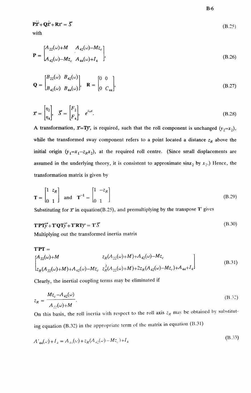
pr+QT+Rr= ~ with
iwt e
B-6
(B.~5)
(B.26)
(B.27)
(B.28)
A transformation, r TY, is required, such that the roll component is unchanged (Y2=X 2),
while the transformed sway component refers to a point located a distance ZR above the
initial origin (y 1=X 1-ZRX 2) , at the required roll centre. (Since small displacements are
assumed in the underlying theory, it is consistent to approximate sinx2 by x z.) Hence, the
transformation matrix is given by
[1 ZR] -1 [1 -ZR] T = and T = o 1 0 1
(B.29)
Substituting for x in equation(B.25), and premultiplying by the transpose T' gives
T'PTy + T'QTy + T'RTY = T'S (B.30)
Multiplying out the transformed inertia matrix
T'PT=
rA22(W)+M
~R(A22(W)+M)+A42(W)-Mzc
zR(Azz(w)+M)+A42(W)-Mzc ]
Z~(A22(W)+M)+2zR(A4Z<W)-Mzc)+A44+[4 (B.3!)
Clearly, the inertial coupling terms may be eliminated if
On this basis, the roll inertia with respect to the roll axis ZR may be obtained by sllbstitllt-
ing equation (B.32) in the appropriate term of the matrix in equation (B.3l)
(B.Y~)
C-1
Appendix C - Derivations for Volterra Functionals
Higher Order Transfer Functions
In this section, expressions are derived for the Fourier transforms of some Volterra ker
nels of order greater than one, here referred to as higher order transfer functions. The
derivation starts from a single degree of freedom differential equation for ship rolling,
including a cubic damping term, and assumed to be written as
AY(t)+B vi (t)+B:J\t)+Cy(t) = x(t) (C.1)
where A,B1,B3,C are constant coefficients.
A Volterra functional series is required, to express the response, y (t), as a functional of
the excitation, x(t), in the form
y(t) = H[rx(t)] 00
n=l
n=oo 00
= :E rn J . .. Jhn(T1, •.. ,Tn)X(t-T1) •.. x(t-Tn)dTl ... dTn (C.2) n=l
-00
where r is an arbitrary constant, Hn (n =1,2, ... ) represent the terms of the senes III
operator notation, and hn (.) are the kernels of the series. The constant r is included to
identify terms of various order in the derivation, and it may subsequently be set to unity.
A shorthand for the terms in the functional series is given by
n=1,2, ... (C.3)
The derivation may conveniently be carried out by utilising the functional series for the
inverse system, as indicated by Schetzen (1980, chp.8). This functional series is expressed
by
x (t) = K[y (t ) ] 00
(CA)
n=l
where Knare the terms of the series for the inverse system. Clearly, the linear. first term
of this series is given by
-1
In operator notation. the required result may be expressed by H = K .
(C.S)
According to

C-2
Schetzen, this inverse exists, provided the inverse of the linear operator (K;l) is stable for
some finite range of excitation amplitude, and this is assumed to be the case in the follow-
mg.
When the functional series (C.2) is substituted into the differential equation (C.I), includ-
ing the factor r on the excitation, it follows that
00 00
n=l n=l 00 00 00
00
(C.6)
By separating and equating terms in like powers of r, the following expressIOns are
obtained
x(t) = AYl(t)+B tYl(t)+CYl(t)
= K1[Yl(t)]
o = K1[Y2(t)]
0= K1[Yit)]+Byi:(t)
0= K1[Yit)]+3Byi:(t)Y2(t)
o = Kl[y5(t)]+3B3rY:(t)Y3(t)+Yl(t)Y~(t)]
(C.7)
(C.B)
(C.9)
(C.lO)
(C.II)
This set of equations may be solved sequentially to the required order. Operating on both
sides of equation (C. 7) by K;l gives
Yl(t) = K;l[X(t)] (C.12)
Similarly from equation (C.B)
1 (C.l3) yit) = K; [0] Hence, it follows that yit ) is identically equal to zero, since any first order kernel gives
zero response to zero input. Continuing in the same manner with equations (C.9) to
(C.II)
Y3(t) = -B3K;1[.Y:(t)] (C.l'+)
Yit) = -3B3K;1[.Y:(t)Yit )]
=0 (C .15)
Ys(t) = -3B3K;1[.Y~(t)Y3(t)+_\'1(Y)Y~(t)] = - 3B 3K;1[.Y: (t)y 3(t)]
Schetzen applies an elegant technique to obtain the higher order transfer functions \'ia box
(C .16)

C-3
diagrams, on the basis of the above expressions. Instead, the underlying anal)1ic expres-
sions are applied here, resulting in a lengthier derivation, but avoiding an explanation of
the box diagram technique. Since the linear response derivative figures in equations (C.l'+)
and (C.16), an additional linear term is introduced, identified by a prime, to handle this
derivative in the following.
00
= J h'l(r)x(t-r)dr (C.17)
-00
Expanding the expression for the trilinear term in equation (C.14), and substituting Hl=K;l
gIves
Y 3(1) ~ - B 3HI [J J J h' I (<7 I)h' I (<72)h 'I (<73)X(I-<7 I )X (1-<72)X (1-<7J d<7l d<72d <7,] -00
00
(C.18)
Applying a change of variable, gives
00
(C.19)
From this expression, the third order kernel may be identified as
00
hirl,r2,T3) = -B3 J h\ (rl-r4)h 'l(r2-r4)h 'l(r3-r4)h l(r4)d r4 (C .20)
-00 • h' d d Frier transform of the third The cubic transfer function is obtamed from the t Ir or er ou
order kernel

C-4
00
-00
00
-00
00
-00
·du ... du 1 4 (C.21)
where a change of variables has again been applied. This multiple integral is clearly separ-
able into 4 simple integrals, which are seen to be the Fourier transforms of first order ker-
nels, leading to linear transfer functions. Hence, the cubic transfer function simplifies to
G3(W1,W2,W3) = -B3G' 1(w1)G' 1(w2)G' 1(w3)Gl(wl+w2+w3) (C.22)
Finally, substituting G' 1 (w )=i wG 1 (w) to obtain the cubic transfer function in a convenient
form
(C.23)
Note that the cubic transfer function is symmetric in its arguments; i.e. it takes the same
value independent of the order of the arguments.
The linear transfer function, obtained from equation (C.l) when B3=O, is given by the stan-
dard result
(C.24)
Next, the fifth order transfer function is derived, using the same procedure as above, but
omitting some of the details. Substituting for Yl(t) from equation (C.l7) in equation
(C.l6), and introducingY3(t)=H'3[x(t)] to handle this derivative, (with associated kernel h'3
and kernel transform G' 3)' leads to

c-s
00
00
00
(C.2S)
The fifth order kernel may now be identified as
00
(C.26)
By taking the fifth order Fourier transform, an expression is obtained for the fifth order
transfer function
00
00
-i[w u + ... +w u +u (w + ... +w )] 11 SS 61 S d d . e T •• , T
1 6
= -3B3G'l(W1)G'l(W2) G'3(W3,W4,WS) G1(W1+ ... +WS)
= 3iB3WIW2(W3+W4+(VS) G1(W1) G1(W2) G3(W3,W4,WS) G1(W1+ ... +WS) (C.27)
this form of the fifth order transfer function is not symmetric, and the - symbol is used to
indicate this. In order to obtain a symmetric version, it is necessary to take the mean of
the different expressions resulting from permutation of the arguments. In this case, 10 dif-
ferent expressions are obtained by selecting 2 of the five arguments of Gs to be the argu-
ments of the first two Gl
terms. Thus, the symmetric form of the fifth order transfer func-
tion may be written as
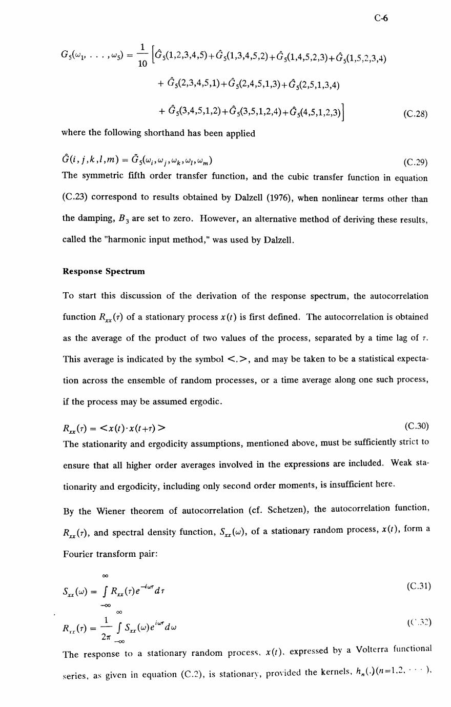
C-6
( 1 [A A GS WI' ••• ,WS) = ~ Gs(1,2,3,4,5)+Gs(1,3,4,5,2)+Os(1,4,5,2,3)+Os(1,5,2,3,4)
+ OS(2,3,4,5,1)+ 0 5(2,4,5,1,3) +Os(2,5,1,3,4)
+ 0 5(3,4,5,1,2)+0 5(3,5,1,2,4)+0 5(4,5,1,2,3)]
where the following shorthand has been applied
(C.28)
O(i,j,k,l,m) = G5(Wi,Wj,Wk,W/,Wm) (C.29)
The symmetric fifth order transfer function, and the cubic transfer function in equation
(C.23) correspond to results obtained by Dalzell (1976), when nonlinear terms other than
the damping, B 3 are set to zero. However, an alternative method of deriving these results,
called the "harmonic input method," was used by Dalzell.
Response Spectrum
To start this discussion of the derivation of the response spectrum, the autocorrelation
function Rxx(r) of a stationary process x(t) is first defined. The autocorrelation is obtained
as the average of the product of two values of the process, separated by a time lag of T.
This average is indicated by the symbol <. >, and may be taken to be a statistical expecta-
tion across the ensemble of random processes, or a time average along one such process,
if the process may be assumed ergodic.
Rxx(r) = <x(t)· x(t +r) > (C.30)
The stationarity and ergodicity assumptions, mentioned above, must be sufficiently strict to
ensure that all higher order averages involved in the expressions are included. Weak sta-
tionarity and ergodicity, including only second order moments, is insufficient here.
By the Wiener theorem of autocorrelation (cf. Schetzen), the autocorrelation function,
Rxx(r), and spectral density function, Sxx(w), of a stationary random process, x(t), form a
Fourier transform pair:
00
(C.31)
-00
00
. d x (t), expressed by a Volterra functional The response to a stationary ran om proces';, -
series. as given in equation (C.2), is stationary, provided the kernels. hn (·)(n=1,2, -' .),

C-7
are time invariant. Convergence and stability requirements are implicit in this statement,
since they are necessary for the existence of the functional series representation. The
autocorrelation function of the response may then be expressed by
Ryy(r) = <y(t)·y(t+r) > 00 00
m=ln=l
= < HI [x(t)]H I [x(t +r)] + HI [x (t)]H2[X(t +r)] +H2[x (t)]H I [x (t +r)]
+HI [x(t)]H3[x(t +r)] +H3[X (t )]HI [x(t +T)] +H2[x(t)]H2[x(t +r)] + ... > (C.33)
In the present case, the approximation of a response by a functional polynomial truncated
after the third term, with even order terms equal to zero, is of primary interest. The
derivation of the response spectrum for this case from the expressions given above is
lengthy. Instead, the result given by Rugh (1981) is quoted, assuming the excitation is a
zero-mean, Gaussian process,
Syy(W) = G I (w)G I (-w)Sxx(w) 00 00
+ :" [GJ(W) J G3(-w,wJ,-wJ)dwJ +GJ(-w) J G,(W,Wl>-WJ)dWJ]S=(W) -00 -00
00
00
(C.34)
The validity of this expression requires the cubic transfer function to be symmetric in its
arguments. Noting that the transfer functions are complex, while the excitation spectra are
real functions, a little complex algebra may be applied to reformulate the expression in a
convenient manner. Denoting complex conjugates by an asterix (*), it is evident from the
Fourier transform relationship between transfer functions and real kernel functions, that
• Gn(-wl' ... ,-wn) = Gn(wl' . .. ,wn)
(C.35)
Hence, the squared modulus of a transfer function is expressed by
2
1 Gn(wl' ... ,wn) 1 = Gn(wl' ... ,wn)·Gn(-wl' ... ,-wn) (C.36)
The following relationship is also applied
'1' 2
IZ 1+ Z::I- = IZll-+Z:Z::+ZIZ;+l z21 (C .37)

C-8
where Zl and Z2 are complex, to obtain
00 2
Syy(w) = I G,(w)+ :" J G3(w,w"-w,)S,,,(w,)dw, I S",(w) -00
00
6 2
+ 2 J J I GiW-WI-W2'Wl'W2) I Sxx(W-WI-W2)Sxx(Wl)Sxx(W2)dwldw2 (27r) -00
(C.38)
This agrees with the expression applied by Dalzell (1976).
Some further simplification is advisable prior to numerical calculation of the response
spectrum. Two parts of the above expression for the response spectrum are considered
Syy(W) = Syl(W)+Sy3(W) 00 2
Syl(W) = I G1(w)+ ~ J GiW'Wl'-Wl)Sxx(Wl)dwl I Sxx(W) 27r
-00
00
6 2
Sy3(W) = J J I GiW-WI-W2'Wl'W2) I Sxx(W-W1-W2) (27r)2 -00
(C.39)
(C.40)
(C.4l)
Substituting the cubic transfer function from equation (C.23) into the integrand of the first
part, Syl(W), gives
(C.42)
Inserting this expression for the cubic transfer function in equation (C.40), and replacing
the two-sided integral by a one-sided integral (since the integrand is an even function of wI)
gIves
3 00 2 2
Syl(W) = I G 1(w)--iB 3wGi(w)J W: I G1(w1) I Sxx(wl)dwll Sxx(W) 7r o
2 2 3 00 2 I
= I G1(w) I ·11--iB3wG 1(w) J W: I G1(w1) I Sxx(w1)dw1 Sxx(w) (C.43) 7r 0
Consider next the cubic transfer function in the integrand of equation (C.4l), and substi-
tute from equation (C.23)

C-9
2
I G3(W-WI-W2,WI,W2) I = G3(W-WI-W2,WI,W2)· G3(-W+WI+W2,-WI,-""'2)
= iB 3( W-W1-W2) WI W2 G I (W-W1-W2) G I (WI) G I (W2) G I (W-W1-W2+W1 +W2)
. iB 3( -W+WI +W2) (-W1)( -W2) G I (-W+WI +W~ G I (-WI) G 1 (-W2)
. GI(-W+WI+W2-WI-W2) 2 2221 121 2 2 2
= B 3 (w-W I-W2) W1W2 G1(W-WI-W2) . G1(WI) I ·1 G1(W2) I ·1 G1(W) I (C.44)
Hence, replacing this expression in equation (C.4l)
2 2
. I G1(w l ) I . I G1(w2) I . Sxx(w-wl-w2)Sxx(wI)Sxx(w2)dwldw2 (C.45)
Note that both input and response spectra are real, even functions, extending from -00 to
00. Hence, ordinates of one-sided spectra are given by twice the ordinates of the two-sided
spectra for positive frequencies. To obtain the spectra dimensioned so that the area under
the spectrum gives the variance, it is necessary to divide the spectra by 21r, as may be seen
by considering the variance as given by R(O) in equation (C.32).


© 1984 The Royal Institution of Naval Architects.
Estimation of Ship Roll Damping Coefficients
by J.B.Mathisen*'(Member) and W.G.Pricet (Fellow)
Originall" Published for Written DisclIssion
SUMMARY: Methods are developed for the estimation of roll damping coefficients from both decay and forced rolling tests. Two nonlinear damping models are considered in a single degree of freedom equation for the roll motion. The damping models are referred to as linear plus quadratic damping and as linear plus cubic damping. The estimation techniques are checked against numerical simulations and applied to model test data. Reasonably good fits to the model test data are obtained for both damping models, with the linear plus quadratic damping model showing some advantage over the, linear plus cubic , damping model.
1. INTRODUCTION
The calculation of wave-induced rigid ship motions by means of various strip theories, as described in Refs. 1-4, has become standard practice in the past decade. All but one of the coefficients of the equations of motion, required by these techniques, can be numerically determined by means of linear potential theory. The exception is the roll damping coefficient. Authors of all the strip theories cited previously have found it necessary to introduce a viscous roll damping term in addition to the linear wavemaking damping, in order to obtain reasonable predictions of the roll motion. Some progress is now being made on the numerical determination of viscous roll damping coefficients (cf. Refs. 5-7), but it seems likely to be several years before generally applicable methods wlll be available. Empirically determined roll damping coefficients are thus required, both in current roll motion predictions, and for the validation of the viscous clamping theories under development.
When only linear damping is conSidered, then the single damping coefficient may be obtained from the logarithmic decrement of a decay test, as indicated by Conolly(S). Current methods for the estimation of linear and nonlinear damping coefficients from decay tests are described by Dalzell(S) and Himeno(10). Basically, these methods equate the loss in potential energy over each cycle of the decay test to the energy diSSipated by damping with an assumed sinusoidal motion at the mean amplitude for that cycle.
This paper presents techniques for the estimation of roll damping coefficients from both roll decay tests and from forced rolling tests. These techniques are believed to represent an improvement on current methods for the analySiS of decay tests, because the concept of a mean amplitude for each cycle is avoided, and the associated approximations are largely eliminated. Two nonlinear mathematical models are conSidered; viz. linear plus quadratic damping, and linear plus cubic damping, in an uncoupled roll equation. Nonlinear roll restoring moments have also been considered in many other papers, but are omitted here in the interest of simplicity. Results obtained on this basis should be useful for the majority of ships in moderate seaways, since the viscous damping term is essential even at fairly small roll amplitudes (Refs.1-4). On the other hand, the nonlinearity in the roll restoring moment is clearly more important in capsizing Situations, and possibly also for ships of unusual form or barges with very low freeboard. A more general approach applicable to the analysis of decay
• A. S. Veritas Research, Hcevik, Norway. t Department of Mechanical Engineering, BruneI University,
Uxbridge, UK.
tests, including nonlinearities in both damping and restoring terms has recently been published by Roberts (11).
Although an uncoupled roll equation is assumed in this paper, it is recognised that the complete linear equations describing wave-induced ship motions include coupling terms between rOll, sway, and yaw. These coupling terms are assumed to be of smaller order of magnitude than the nonlinear roll damping terms included here. This Simplifies the experiments and the analysis. There is some additional justification for this assumption in the case of roll decay and forced rOlling tests, as opposed to the case of wave-induced motions, since there is no external excitation of the sway and yaw motions in these tests. Hence, the sway and yaw motions will be relatively small, and the coupling effects correspondingly reduced. However, these neglected coupling terms may be of greater magnitude than some of the higher order terms included in the present perturbation analysis of roll decay tests, though a discussion of the relative magnitudes of such terms is omitted from this paper.
Ship rolling is recognised to be a strongly r~sonant motion. This implies that the roll damping is subcritical. Advantage will be taken of this fact in assuming that the linear damping coefficient is small relative to twice the natural frequency, as will be discussed in Section 3. 1.
2. MATHEMATICAL MODEL
The uncoupled mathematical model of ship rolling, as discussed previously, may be assumed written in the simple form
Ax + l3(i) + Cx = F (1)
where ~ is the roll angle, A is the inertia coefficient (dry structure plus fluid component), C is the restoring moment coefficient, and F is the excitation moment. Two alternative forms are considered for the damping function (13)
132 = Dlx + D2x I.l-I 133 = Blx + B3x3
(2)
(3)
referred to as linear plus quadratic damping and linear plus cubic damping respectively. From phYSical ~easoning it is assumed that all the linear coefficients (A BCD ) ~re positive, and the inertia and damping coeffici!~t~ m~y be frequency dependent. The intention is to derive methods of estimating the damping coefficients from experimental data.
295

ESTIMATION OF -SHIP ROLL DAMPING COEFFICIENTS
In order to simplify the algebra slightly, the inertia coefficient Is eliminated, and the two versions of the equation of motion are rewritten as
where b l = BI/A, £b 3 = B3IA, c = CiA = wfi, d l = DI/A, Ed2 = D21 A, f = F I A and Wn denotes the undamped natural frequency of the ship or model. The small parameter t
(4)
(5)
(0<£< 1) is included for use in the perturbation expansion below, indicating that the nonlinear damping moment terms are assumed to be smaller in magnitude than the linear damping moments. This will always be the case for non-zero linear damping and sufficiently small roll velocities.
3. ROLL DECAY
In a roll decay test, the ship or ship model is first given some initial roll displacement by static or dynamic means. The external moment is then removed, and the gradual decay of the roll motion is recorded. This corresponds to an initial value problem in equation (1), with zero excitation (F = 0).
To describe this roll motion, a perturbation solution is sought in the form of a power series in the small parameter, E. That is,
(6)
where t represents time, "0 is referred to as the basic solution, \'1 as the first order term, etc. The initial roll displacement is defined at time t = 0,
3.1. Decay with linear plus quadratic damping
This case corresponds to equation (4) with f = O. The perturbation expansion (6) is inserted into equation (4) and equations are separated in powers of E in the form
~o + dlxO + cXo = 0,
Xl + dl ~l + Ct"l = - ti2i~sJ!n(.~0),
x2 + til ~2 + CX 2 = - d2.YOY1sgn('YO+EXl)',
(7)
(8)
(9)
These equations may be solved sequentially to any desired order. The right hand sides of the equations may effectively be viewed as excitation terms, defined by the lower order solutions. The sgn (or sign) function is introduced to eliminate the absolute value involved in the quadratic damping term, and is defined by
\ +1, \'>0 sgn(x) = \ 0, ,\,=0
'-l,x<O (10)
In deriving equations (7-9), sgn(x) has been approximated by using only the terms of the expansion (6) appropriate to the order of the particular equation. For example, in deriving equation (8) to the first order in E we observe that
£d2x2 sgn(xo + E'~l + £2X2 + •.• ) "" Ed2.Y~sgn(.Yo). (11)
Subcritical dampin!! (d~ < 4c) is characteristic for ship rolling, giving the familiar solution to equation (7) in the form
(12)
wher.e XOI and 801 are constants determined by the initial condItions. The phase angle (801 ) is eliminated in the following analYSis by suitable choice of the time origin; i.e. t = 0 is at the first maxima or minima included in the decay analysis. Note that X01 is not equal to the value of the first roll maxima or minima included, but rather the initial
296
amplitude of a purely linear decay process. The roll velocity due to the basic solution is required in the determination of the right hand side of equation (8). It is obtained by differentiation of equation (12) and is given by
(13)
In order to simplify the phase angles in the followinr; analysis, we apply the assumption that the linear damping coefficient is small compared to twice the natural frequency. This is consistent with the previous subcritical damping assumption so that equation (13) simplifies to
(14)
After substituting this expression for the roll velocity, the right hand side of equation (8) may conveniently be expanded as an odd Fourier series in the form
8 sin(PWnI)
7IP(P + 2)(P- 2)' (15)
The homogeneous solution to equation (8) takes the same form as the basic solution, equation (12), and need not be considered separately. Thus, only a particular integral is required. Considerinp; only the first harmonic term of this Fourier series in the excitation of equation (8), the first harmonic of the response is then in phase with the basic solution given in equation (12), with an amplitude
8d2 wn Xu = -- X2 e-dlt 3rrril
01 • (16)
This amplitude decays twice as quickly as the basic amplitude, and now also involves the quadratic damping coefficient. The response to the higher harmonics of the Fourier series (15) may be neglected in comparison with the response to the first harmonic. There are two reasons for this: (a) the higher harmonic excitations have small amplitude compared to the first harmonic, and (b) the first harmonic occurs at the natural frequency in the decay test, and the strongly resonant roll response will tend to filter out higher frequency excitations.
By continuing the above analysis to higher orders of E it quickly becomes apparent that the amplitude terms of 'the solution form a geometric series. Summation of this series gives
(17)
This summation is valid for all t ~ 0 provided that the following convergence criterion, based on the common ratio of the geometric series, is satisfied. That is
SEd2XOl wn --3~ < 1, t ~(). (1S)
This condition corresponds to the initial assumption that the nonlinear damping moment is less than the linear damping moment, if harmonic rolling with frequency wand amplitude 8X 01 1(371) is considered. n
In accordance with the usual analysis of roll decay data we wish only to consider the sequence of absolute values of roll maxima and minima ~r, r = 0, 1, 2, ... ThiR sequence is simply obtained from the time function in equation (17) by setting
1= rrr/w,l> r = 0,1,2, ... (19)
and takes the form
_ 3rrd1XOl ~r-----.~~~------
3rrd1exp{~1::} - 8td2X01 wn (20)
)

The undamped natural frequency (Wn) may be taken as the mean frequency of the decay record. If significant, systematic variation in the frequency is apparent during the decay proceSS then this is an indication that analysis by this technique may 'be inappropriate. There remain three unknowns in equation (20), XOI ' dl , and €d2 • Hence, at least three roll maxima and minima must be available from a decay test to provide estimates for these three parameters. A much larger number of maxima and minima will usually be available in practice, and some form of curve fitting technique is appropriate to minimise the effect of random error.
An appropriate error term Or may be defined as
6 r = ~rOBS - Er EST (21)
which determines the difference between the observed roll extrema (~roBs) and the calculated value (~rEST) obtained using estimates of the unknown parameters in equation (20). The sum of the squared error terms (i.e. ~6~) is referred
T
to as the residual sum of squares, and minimisation of this function leads to optimal estimates of the damping coefficients. The residual is a fairly complicated, nonlinear function of the three parameters (XOI ' dl , €d2 ) and may have a number of local minima. Some care may be necessary to ensure that the minimum most appropriate to the present problem is found. For example, a nonlinear least-squares technique was tried initially, but occasionally resulted in a negative value of the linear damping coefficient. Such negative values are not believed to be physically realistic, and may be due to the effects of experimental errors. Some form of constrained minimisation technique is therefore to be preferred, with the constraint limitinll; the linear coefficient to positive values. After estimatin~ the parameters, it is necessary to check that the convergence criterion given in equation (18) is satisfied. If this is not the case, then the largest roll angle must be omitted from the decay data, and the numerical estimation repeated.
The value of the inertia (A) is required to convert to the normal form of the damping coefficients (D I , D2 ). The inertia may be estimated from the natural frequency and the restoring coefficient (C), determined from the transverse metacentric height (GM) and displacement weight (V') of the vessel, since
(22)
3.2. Decay with linear plus cubic damping
ThiS case corresponds to equation (5) with f = O. The perturbation expansion (6) is inserted into equation (5) and the equations are again separated into powers of (. The resulting series of equations is as follows:
-"0 + bl-"o + c'"o = 0,
"1 + b1-"1 + C'"l = - b3"~,
·"2 + b1 "2 + CX2 = - 3b3i-~~1'
(23)
(24)
(25)
The left hand sides of equations (23-25) correspond closely to equations (7 - 9), but the form of the right hand side s is different due to the different damping model. The solution is simplified somewhat for this model, since it is not necessary to introduce the sgn function nor a Fourier series expansion. The basic solution again takes the same form as in equation (12). That is
(26)
Proceeding as previously, the phase (801 ) is set to zero, and the roll velocity is Simplified as in equation (14) with the assumption that the linear damping coefficient is small relative to twice the natural frequency. Substitutlon into the
ESTIMATION OF SHIP ROLL DAMPING COEFFICIENTS
TABLE Y. Coefficients gp of the series defined by equation (29)
p gp
0 l' 0
1 0'375
2 O· 21093750
3 0'13183594
4 O' 08651733
5 0'0583992
6 0'04014945
7 0'02796122
8 0·01966024
9 0'01392600
10 O'{)O992228
right hand side of equation (24) provides an excitation comprising first and third harmonic terms in the form
If we consider only the first harmonic term of this 'excitation', the first harmonic of the response is then in phase with the basic solution (26), with amplitude
3b X3 ht~ X - 3 01 -'1 -3b 1//2
11 - 8b e • 1
(28)
Tn this case the amplitude decays three Umes as quickly as the basic solution amplitude, and now involves the cubic damping coefficient. The response to the third harmonic term in the excitation, equation (27), is neglected with the same reasoning presented in Section 3.1. By continuing the above analysis to higher orders of E, it becomes apparent that the solution may be expressed as the summation of a series in the following form
where the calculated values of the coefficients gp are given in Table t, and the summation is taken to the k-th order in E.
Since the values of the exponential terms are ~ 1 for all t :;, 0, and the values of the coefficients (gp) decreasing, convergence of this series is obtained for all t;. 0 provided that
(30)
This condition corresponds to the initial assumption that the nonlinear damping moment is less than the linear damping moment, if harmonic rolling with amplitude X and frequency "11 is considered. The sequence of absolute v~tues of roll maxima and minima is obtained from the time function in equation (29) by substituting for t from equation (19) and given by
k
~r = P~O [gpX01(Eb3XniwIVbl)Pe-<2P+liJ1YTT/(2Wn>1. (31)
A constrained minimisation technique, as discussed in Section 3.1, is again appropriate to estimate the Wlknown parameters Xol,l) l' and f.b 2 from equation (31). After estimating the parameters, it is necessary to check that the convergence criterion given in equation (30) is satisfied.
297
ESTIMATION OF SHIP ROLL DAMPING COEFFICIENTS
4. FORCED ROLLING
Forced rolling tests are usually performed in one of two different ways:
(a) Monofrequency motion Monofrequency, sinusoidal roll motion is imposed, with the other degrees of freedom restrained, and the necessary exciting moment is recorded. This type of test is only performed at model scale, with motion imposed by hydraulic servo-actuators, or Scotch-yoke mechanisms as described in Ref. 12. The roll axis must be fixed in this case. Its location will affect the results, and should be taken into account if the damping coeffiCients are subsequently used in a prediction model.
(h) Monofrequency excitation A monofrequency, sinusoidal roll forCing moment is applied and the resulting roll motion is recorded. In model tests, this excitation is usually generated by means of rotating weights, or precessing gyroscopes as described in Ref. 13. At full scale, with forward speed, this type of excitation may be approximated by appropriate control of fin stabilisers or rudders.
Harmonic analysis of the response signal is required in both cases including accurate determination of the phase angles betwe~n exciting moment and roll response. The analysis of these two types of forced rolling tests will be considered separately in the following diSCUSSions.
4.1 Monofrequency motion
In this case the prescribed motion may be expressed as
x(t} '" Xl cos(wt} (32)
where Xl is the amplltude, and w is the frequency of the excitation. The exciting moment is then Simply obtained by substituting the prescribed motion into the equation of motion (1), with the chosen damping model.
4.1.1 Linear plus quadratic damping
Substituting equation (32) into equation (I) with the linear plus quadratic damping model (2), and applying a Fourier expansion to the quadratic term gives
F = (C - Aw2)Xl cos(wt) - (DlX1 w
+ :. D2X~w2) sin(wt)
+ D2X~w2 ~ 8 sin(pwt) P=3,5,'" Trp(P + 2)(p- 2)
(33)
An estimation scheme to evaluate the damping coefficients is easily derived from this equation. The quadratic damping coefficient (D2 ) may be obtained by equating the amplitude of the third harmonic of the exciting moment (F 3) with the third harmonic term in equation (33), giving
(34)
USing the value of the coeffiCient, an expression for the linear damping coefficient (D l ) may be found by equating the out-of-phase first harmonic component of the exciting moment with the first harmonic sine term in equation (33). This coefficient is then given by
(3S)
where F 1 is the amplitude of the first harmonic of the exciting moment, and 1/1 1 is the associated phase angle.
298
4.1.2 Linear plus cubic damping
Substituting equation (32) into equation (1) with the linear plus cubic damping model, equation (3), gives
3 F ::::: (C - Aw2)Xl cos(wt) - (BlXl W + '4 B3X~w3) sin(wt)
(36)
A technique to estimate these damping coefficients is again easily derived from this equation. An expression for the cubic damping coefficient (B 3 ) Is obtained by equating the amplitude of the third harmonic of the exciting moment (F 3) with the amplitude of the third harmonic term in equation (36), and it follows that
(37)
USing the value of this coeffiCient, and equating the out-ofphase component of the first harmonic of the exciting moment with the first harmonic sine term in equation (36) provides an expression for the linear damping coefficient (B l ), that is
(38)
The presence of Significant amplitudes for other than the first and third harmonics of the exciting moment would imply either inadequacy in the present mathematical model for the roll motion, or possibly experimental error. If experimental errors can be ruled out as the primary source of such higher harmonics, then the present mathematical model would require further refinement.
The accuracy of the estimate for the linear damping coeffiCient will be dependent on the magnitude of the out-oC-phase first harmonic exciting moment, and consequently on the phase angle (1/1]). This phase angle is likely to b.e small for frequencies far from resonance, and it may be difficult to obtain useful estimates for the linear damping coefficient at such frequencies. However, near resonance the phase angle (\VI) approaches "/2.
4.2 Monofrequency excitation
In this case the exciting moment may be written as
F(t) '" F 1 cos(wt) (39)
where Fl is the excitation amplitude, and w is the forCing frequency. The steady- state solution to equation (1) is required for the two different damping models. In either case, and as a generalisation, the periodic solution may be represented as a Fourier series in the form
k x(t)::::: L; Xp cos(pwl + Bp)
P=l (40)
where Xp are the amplitudes of the harmonic components of the roll response, ep are the phase angles, and k is the number of terms obtainable from the experimental results with acceptable accuracy.
Now the net energy absorbed by the rOlling ship system in one cycle of the excitation may be expressed as
w::::: J F(t) dr cycle
211/W k ::::: - F1w r. cos(wt) L PXp sin(pwt +ep) dt. (41)
'0 P"'l
The orthogonaltty relationship associated with the Fourier series leads to a result of this integration where only the first harmonic term of the roll motion (p '" 1) is present.

That is the expression for the energy absorbed reduces to
(42)
The energy dissipated by the system due to the damping terms is considered next, The dissipation due to the ~inear damping term will have the same form for both dampmg models, and is given by
El = J B1rd'( cycle
21T/W Ii , = Bl .r. [-w L: PXp sin(pwt + 8p»)2 rit
o P=1
k = B t1TW L; (pXp)2
P=l (43)
where Dl replaces Bl for the quadratic damping model. The algebra required to keep the full Fourier series representation of the roll response becomes cumbersome for the energy absorbed by the nonlinear damping terms, and some simplification is deSirable. Experience indicates that the response in this type of test is very well represented by the fir st harmonic term only, This was certainly the case for the model test results analysed in Section 6, and in the numerical simulations discussed in Section 5, Perturbation analysis, as applied in Ref. 14, also indicates that there will be very little response at higher harmonics, except for excitation at sub-harmonics of the resonance frequency, Although an analysis was undertaken including both first and third harmonics, it was found that the inclusion of the higher harmonic term had inSignificant influence on the results, Accordingly, as a justifiable Simplification, only the first harmonic of the roll response will be retained in the following analysis of the energy dissipation,
4.2.1 Linear pillS quadratic damping
The energy diSSipated by the quadratic damping term during one response cycle is now given by
E2 = r D2·Ylk I dx cy'i:le
2!T/W
= D2 fo 12 \'~I dt
8 "" 3" D2X~w2 (44)
and the energy absorbed by the shIp model may be equated with the energy diSSipated over one cycle at steady state, Thus, using the expressions in equations (42-44) it follows that
(45)
and
(46)
At least two tests at different excitation amplitudes and constant frequency are necessary to determine the damping coefficients (D1 and D2 ). Usually a larger number of such tests (i,e, amplitude variation) is carried out at each constant frequency, and a least squares technique may then conveniently be applied to estimate the coefficients from the test results, As discussed previously, an error term may be formulated as
where the suffix r indicates results from test yat constant frequency, Minimisation of the sum of the 8luared error
ESTIMATION OF SHIP ROLL DAMPING COEFFICIENTS
terms leads to the following estimators for the damping coefficients
where all the summations are taken over the number of experiments (Index r),
4.2 2 Linear plus cubic damping
The energy dissipated by the cubic damping term during one roll cycle is given by
E3 = f B 3·,,3 dr: cycle
21T/W
= B3 fo x4 dt
Again the energy absorbed may be equated to the energy diSSipated over one cycle at steady state, Combining this expression with equations (42-43) it follows that
w= El + E3
and
(50)
(51)
Applying a least squares technique in the same manner as in the quadratic case leads to the following estimators for these damping coefficients
LXhLFlrXlysin(-61r) - LXtrLFlrX~r B -1 - w[LX¥YLX~r - {LXfr)2] (52)
4[~X¥r~F lrX~r - Lxty~F lrXlr] B -3 - 3w3[LX~rtX~r - (6xtr)2] (53)
where the summations are again taken over the set of tests carried out with constant frequency and varying excitation amplitude (index r), This process may be repeated at each prescribed frequency of oscillation and the analysiS does not preclude the possibility that the damping coefficients may vary with frequency,
TABLE n, A comparison of damping coefficients used as input to numerical simulation with results estimated from the output
Input Estimates
roll
decay
, forced
rolling
W = 3'22rad/s
Linear plus quadratic damping model
Dl [Nms/rad]
D2 [Nm(s/rad)2]
0' 5119 0' 5073
3'427 3'446
Linear plus cubic damping model
Bl [Nms/rad]
B3 [Nm(s/rad)3]
1'472
2'539
1'470
2'560
0'5160
3'424
1'478
2'525
299
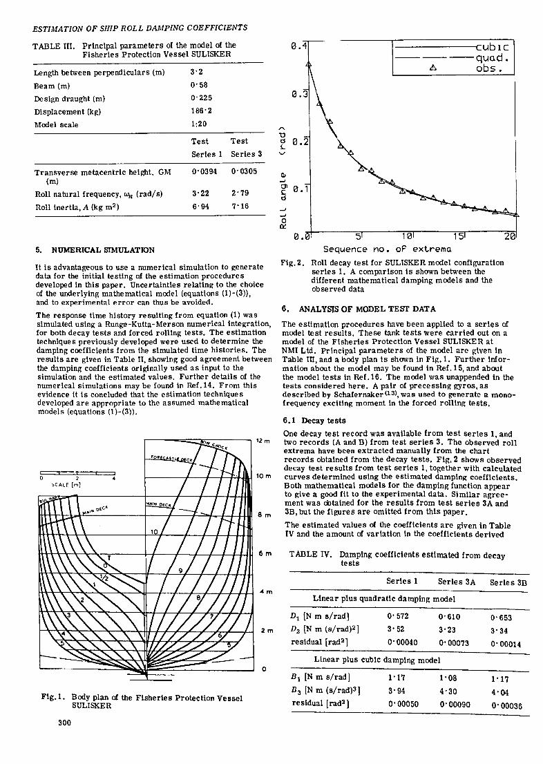
ESTIMATION OF SHIP ROLL DAMPING COEFFICIENTS
TABLE III. Principal parameters of the model of the Fisheries Protection Vessel SULISKER
Length between perpendiculars (m)
Beam (m)
Design draught (m)
Displacement (kg)
Model scale
3'2
0'58
0'225
186'2
1:20
Test Test
Series 1 Series 3
Transverse metacentric height. GM (m)
Roll natural frequency, Wn (rad/s)
Roll inertia, A (kg m2)
5. NUMERICAL SIMULATION
0'0394 0' 0305
3'22 2'79
6'94 7'16
It is advantageous to use a numerical simulation to generate data for the initial testing of the estimation procedures developed in this paper. Uncertainties relating to the choice of the underlying mathematical model (equations (1)-(3)), and to experimental error can thus be avoided.
The response time history resulting from equation (1) was simulated using a Runge-Kutta-Merson numerical integration, for both decay tests and forced rolling tests. The estimation techniques previously developed were used to determine the damping coefficients from the simulated time histories. The results are given in Table II, showing good agreement between the damping coefficients originally used as input to the simulation and the estimated values. Further details of the numerical simulations may be found in Ref. 14. From this evidence it is concluded that the estimation techniques developed are appropriate to the assumed mathematical models (equations (1 )-(3)).
,---=-;;;;:;;=:1;0;;;--:-----, 12 m
f----+--+~yq..31 10 m
8m
0.4 ------------~CUblC ------qua.d.
A obs.
,.... "0 d L ....,
<II -oJ
0'1 C d
-oJ ..J
0 ~
0.0 5 10 15 Sequence no. of extrema
Ftg.2. Roll decay test for SULISKER model configuration series 1. A comparison is shown between the different mathematical damping models and the observed data
6. ANALYSfS OF MODEL TEST DATA
20
The estimation procedures have been applied to a series of model test results. These tank tests were carried out on a model of the Fisheries Protection Vessel SULISKER at NMI Ltd. Principal parameters of the model are given in Table m, and a body plan is shown in Fig. 1. Further information about the model may be found in Ref. IS, and about the model tests in Ref. 16. The model was unappended in the tests considered here. A pair of precessing gyros, as described by Schafernaker(13), was used to generate a monofrequency exciting moment in the forced rolling tests.
6.1 Decay tests
One decay test record was available from test series I, and two records (A and B) from test series 3. The observed roll extrema have been extracted manually from the chart records obtained from the decay tests. Fig.2 shows observed decay test results from test series I, together with calculated curves determined using the estimated dampinl/; coefficients. Both mathematical models for the damping function appear to give a good fit to the experimental data. Similar agreement was obtained for the results from test series 3A and 3B, but the figures are omitted from this paper.
The estimated values of the coefficients are given in Table IV and the amount of variation in the coefficients derived
6 m T ABLE IV. Damping coefficients estimated from decay tests
Fig.l. Body plan of the Fisheries Protection Vessel SULISKER
300
4m
2m
o
Series 1 Series 3A
Linear plus quadratic damping model
Dl [N m s/rad] o· 572 0'610
D2 [N m (s/rad)2] 3' 52 3'23
residual [rad2 ] 0'00040 0'00073
Linear plus cubic damping model
B1 [N m s/rad]
B3 [N m (s/rad)3]
reSidual [rad2 ]
1'17
3'94
0'00050
1'08
4'30
0'00090
Series 3B
0'653
3'34
0'00014
1'17
4'04
0'00036

0.4
0.3
" "0 d L
-.J
0.2 QI "0 :l ...,
..... -' 0. 0.1 E d
-' -' 0 0:
Fig. 3•
-------------rcubic ------quad.
A obs. 3 5
(excit.mom.amp.).sin<phase) <Nm)
Forced rolling test for SULISKER model configuration series I, at osctllatory frequency w = 3' 2 rad/ s. A comparison is shown between the different mathematical damping models and the observed data
from the three decay tests does not appear excessive. However, the values of the reSidual sum of squares remain slightly smaller for the linear plus quadratic damping model in all the tests. This residual indicates an error variation between the estimated pOints and the observed data, as discussed in Section 3.1.
It is interesting to note the variation in the results for test series 3A and 3B in Table IV. These tests were performed for the same model configuration. but slightly differing initial conditions. This variation is indicative of the random error associated with decay tests.
Table IV also Shows the estimated values of the linear coefficients derived for the two mathematical models to differ widely-as should be expected.
ESTIMATION OF SHIP ROLL DAMPING COEFFICIENTS
the amplitude of the first harmonic since the difference between them appeared to be insignificant. Both mathematical models again appear to give a reasonably good fit to the data in Fig. 3. Similar agreement was also obtained for tests performed over a narrow frequency range about the resonance frequency used in Fig. 3. Comparable results were obtained for test series 3. From an analysis of these data there exists limited evidence suggesting that all the damping coefficients show a dependence on frequency of oscillation. However, additional experimental investigations and analysis are required before this observation can be confirmed. The estimated values of the coefficients are given in Table V for test series 1 and 3, for the chosen frequencies nearest to the natural frequencies. Values of the residual sum of squares are again smaller for the linear plus quadratic
1 .8 E9 ----6---
" "0 d L
01 81
" ~~ IfI 1 .2 E z flJ-~ ...."
0 r~ ~
L 0.6 0
CD
0.0 0.1 0.2 0.3 0.4
(a) Largest roll angle (rad)
12. 5 \ E9
02 ---6--- 83
6.2 Forced rolling tests 10. ~l
0 ~~ Fig.3 shows observed monofrequency excitation forced roll-ing results for test series I, together with curves determined using the damping coefficients estimated from these tests. The amplitude of roll from these tests was used rather than 7. 5 ~ ~~ T ABLE V. Damping coefficients estimated from forced
rolling tests
Series 1 Series 3
w = 3'2 rad/s w=2'85 rad/s
Linear plus quadratic damping model
D1 [N m s/rad]
D2 [N m (s/rad)2]
residual [(Nm)2]
O' 512
3'43
0'018
Linear plus cubic damping model
Bl [N m s/rad]
B3 [N m (s/rad)3]
residual [(Nm)2]
1'47
2' 54
0'144
O' 525
3'34
0'012
l' 58
2'35
0'056
N o
I... o
M CD
(b)
5. 0
2 .5
.0 0.11 0.21 tl 0.3 Largest roLL angLe (rad)
e. 4
Fig.4. Variation of damping coefficients with roll amplitude from decay test series 3B.
(a) Linear coefficients B1 and D1 [Nms/rad]. (b) Non-linear coefficients B3 [Nm(s/rad)31 and
D2 [Nm (s/rad)2].
It is noticeable that coefficients D 1, D2 show less variation with amplitude than B 1• B3
301
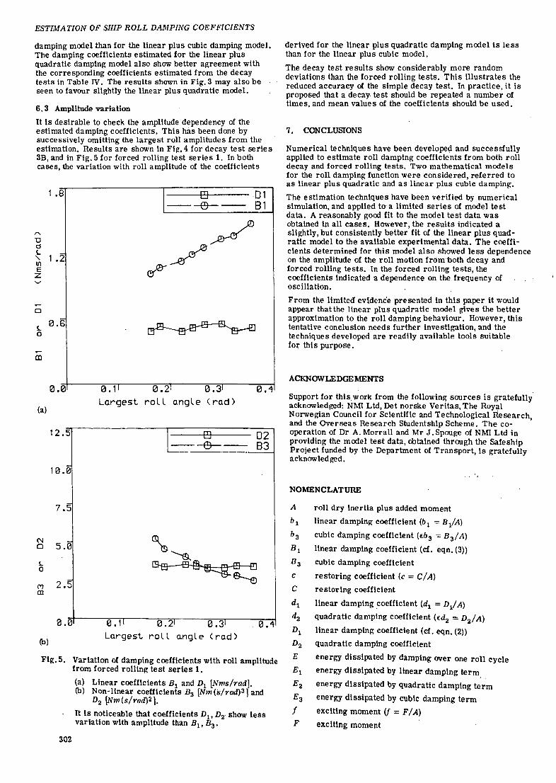
ESTIMATION OF SHIP ROLL DAMPING COEFFICIENTS
damping model than for the linear plus cubic damping model. The damping coefficients estimated for the linear plus quadratic damping model also show better agreement with the corresponding coefficients estimated from the decay tests in Table IV. The results shown in Fig.3 may also be seen to favour slightly the linear plus quadratic model.
6.3 Amplitude variation
It is desirable to check the amplitude dependency of the estimated damping coefficients. This has been done by successively omitting the largest roll amplitudes from the estimation. Results are shown in Fi~. 4 for decay test series 3B, and in Fig. 5 for forced rolling test series 1. In both cases, the variation with roll amplitude of the coefficients
,.... 1) d
1 .B
~ 1.2 III E Z
a
So.. 0.6
a
CD
0.0
(a)
12.5
10.0
7.5
N 5.0 a
!.. 0
("I) 2.5 CD
0.0
(b)
Fig.5.
302
I ~D1
---6--- 81
0.11 0.21 0.31 0.4 Largest roL l angle (rad)
0.11 0.21 0.31 0.4 Largest roll angle (rad)
Variation of damping coefficients with roll amplitude from forced rolling test series 1.
(a) Linear coefficients B1 and D1 [Nms/rad]. (b) Non-linear coefficients B3 [Nm(s/rad)31 and
D2 [Nm(s/rad)2].
It is noticeable that coefficients D1 , D2 show less variation with amplitude than B1 , B3 •
derived for the linear plus quadratic damping model is less than for the linear plus cubic model.
The decay test results show considerably more random deviations than the forced rolling tests. This illustrates the reduced accuracy of the simple decay test. In practice, it is proposed that a decay. test should be repeated a number of times, and mean values of the coefficients should be used.
7. CONCLUSIONS
Numerical techniques have been developec;l and successfully applied to estimate roll damping coefficients from both roll decay and forced rolling tests. Two mathematical models for the roll damping function were conSidered, referred to as linear plus quadratic and as linear plus cubic damping.
The estimation techniques have been verified by numerical Simulation, and applied to a limited series of model test data. A reasonably good fit to the model test data was obtained in all cases. However, the results indicated a slightly, but consistently better fit of the linear plus quadratic model to the available experimental data. The coefficients determined for this model also showed less dependence on the amplitude of the roll motion from'both decay and forced rOlling tests. In the forced rolling tests, the coefficients indicated a dependence on the frequency of oscillation.
From the limited ev\dence presented in this paper it would appear thatthe linear plus quadratic model gives the better apprOXimation to the roll damping behaviour. However, this tentative conclusion needs further investigation, and the techniques developed are readily available tools suitable fo~ this purpose.
ACKNOWLEDGEMENTS
Support for this,work from the following sources is gratefully acknowledged: NMt Ltd, Det norske Veritas, The Royal Norwegian Council for Scientific and Technological Research and the Overseas Research Studentship Scheme. The co- ' operation of Dr A. Morrall and Mr J. Spouge of NMl Ltd in providing the model test data, obtained through the Safeship Project funded by the Department of Transport, is gratefully acknowledged.
NOMENCLATURE
A roll dry inertia plus added moment
b1 linear damping coefficient (b 1 = BiA)
b3 cubic damping coefficient (t:b 3 == B3/A)
B1 linear damping coefficient (cf. eqn. (3»)
B3 cubic damping coefficient
c restoring coefficient (c = C/ A)
restoring coefficient
linear damping ,coeffiCient (d1 = Di A)
quadratic damping coefficient (€d2 = D2/A)
linear damping coefficient (c!. eqn. (2»
quadratic damping coefficient
energy dissipated by damping aver one roll cycle
energy dissipated by linear damping term
energy dissipated by quadratic damping term
energy dissipated by cubic damping term
exciting moment (f :: F / A)
exciting moment

Fp
gp
t
W
p-th harmonic of excltlng moment
constants (cf. Table I)
time
excitation energy absorbed in one roll cycle
roll angle (rad.) x term I of perturbation expansion for roll angle
roll amplitude for order i and harmonic j
p-th harmonic of roll response
damping function
error term for r-th decay extrema, or forcing amplitude
small parameter used in perturbation expansion
9ij phase angle for order i and harmonic j roll decay
9p phase angle for p-th harmonic roll response
1/Ip phase angle for p-th harmonic exciting moment
~r absolute value of r-th roll extrema from decay test
(r = 0,1,2, ... )
w frequency
Wn natural frequency
REFERENCES
1. Salvesen, N., Tuck, E .0., and Faltinsen,O.: 'Ship Motions and Sea Loads', Trans. SNAME 78,1970,303-321.
2. Vugts, J. H.: 'The Hydrodynamic Forces and Ship Motions in Oblique Waves', Netherlands Ship Research Centre TNO, Report 150S, 1971.
3. Raff, A. T.: 'Ship Structural Response in Waves-Program Scores', Ship Structure Committee, report SSC-230, 1972.
4. Fukuda, J., Nagamoto, R., Konuma, M., and Takahashi, M.: 'Theoretical Calculations on the Motions, Hull Surface Pressures and Transverse Strength of a Ship in Waves' Memoirs of the Faculty of Engineering, Kyushu ' University, Vol. 32, No.3, Jan.1973.
5. Bearman, P.W., Downie, M.J., and Graham, J. M. R.: 'Calculation Method for Separated Flows with Applications to OSCillatory Flow Past Cylinders and Roll Damping of Barges', Proc .14th Symp. on Naval Hydrodynamics, Ann Arbor, Michigan, 1982.
6. Patel, M. H., and Brown, D. T.: 'The Calculation of Vorticity Effects on the Motion Response of a FlatBottomed Barge to Waves', Proc. Tntl. Symp. on Hydrodynamics In Ocean Engng., Norwegian Inst. of Tech., Trondhelm, 1981, p. 667.
7. Ikeda, Y., and Tanaka, N.: 'On Viscous Drag of Oscl.llating Bluff Bodies', 12th Scientific and Methodological Seminar of Ship Hydrodynamics, Varna, 1983.
8. Conolly, J. E.: 'Rolling and Its Stabilisation by Active Fins', Trans. RTNA 111,1969,21-48.
9. Dalzell,J. F.: 'A Note on the Form of Ship Roll Damping', Journal of Ship Research 22, No.3, Sept. 1978, 178-185.
10. Himeno, Y.: 'Prediction of Ship Roll D'mpin~A State of the Art', Dept. of Naval Architecture and Marine Engineering, Report no. 239, Sept.1981, Univ. of Mlchigan, Ann Arbor, Michigan.
11. Roberts, J. B.: 'EsUmation of Non-llnear Ship Roll Damping from Free-Decay Data',NMl Ltd. Report R164, 1983.
12. Fujii, H., and Takahashi, T.: 'Study on Lateral Motions of a Ship in Waves by Forced Oscillation Tests', Mitsubishi Technical Bulletin Vol. 87, Aug. 1973, pp.I-14
ESTIMATION OF SHIP ROLL DAMPING COEFFICIENTS
13. Schafernaker, A. S.: 'The NMl Roll Moment Generator\ NMl Ltd. Report R128, 1982.
14. Mathisen,J.B.,and Price,W.G.: 'Determination of Linear plus Cubic Ship Roll Damping Coefficients', NMl Ltd. Report 187, 1984.
15. Morrall, A., and Schafernaker, A. S.: 'Safeship Project 8 Model Experiments-National Maritime Institute', Safeship Seminar, London, March 1982, organised by the National Maritime Institute for the Department of Transport,I72-190.
16. Private communication of model test results for the SULISKER. To be published by NMl Ltd.
WRITTEN DISCUSSION
Dr Y. Ikeda: As shown in the recent works on viscous force acting on oscillating bluff bodies, the drag and added mass coefficients depend on Keulegan-Carpenter number (=UmaxT /D, Umax:maximum speed of motion, T: period, D: representative length). In sinusoidal oscillations, the Keulegan-Carpenter number means a relative amplitude of the motion. The drag coefficient of a bilge keel signUicanUy depends on the Keulegan-Carpenter number too as pointed out in our papers(17, 18). Therefore the damping coefficients D2 or B3 in equations (2) and (3) can not be regarded as being amplitude independent. For this reason I think it is generally impossible to determine the coefficients in equations (2) and (3) from the data measured by a free roll test and a monofrequency excitation test in the strict sense. More detailed discussions on this problem were contained in my recent paper(19). Only for the case when the viscous effect is small, for example, for a ship without bilge keels and with round hull shape, wlll the proposed technique be applicable.
Fortunately, the experimental data used in authors' paper are those for a round vessel without appendages. As shown in our paper(20), the coefficient of the eddymaking damping for 'a naked hull is regarded as amplitude independent in practical usage. Therefore the analysis technique proposed in this paper may be appropriate to this case.
If it is necessary to determine the most resonable form of the roll damping of a ship, I think that the forced rolling test of monofrequency motion which is shown in Section 4.1 is suitable for this purpose. Systematic experiments have to be carried out for various amplitudes and frequencies to identUy the most reasonable form of the roll damping. A free roll test is suitable for obtaining the equivalent linear damping at moderate roll amplitudes.
I wonder whether or not the dUference of the expressions of the nonlinearity in the roll damping is important in the practical analysis of ship roll motion, since the well known non-linear characteristics of roll motion at reasonance mainly caused by the non-linearity of the restoring moment, and the effect of the form of the non-linearity of roll damping on the characteristics may not be so significant. If different roll damping forms, for example equations (2) and (3), have the same energy dissipation for one cycle, a significant dUference of the roll motion may not occur. Therefore I think the equivalent linear damping which depends on the roll amplitude and frequency is convenient for the assessment of the non-linear characteristics of the roll motion except at extreme amplitudes.
For large amplitude roll motion, the expression of nonlinearity of the roll damping may play an important role. In this case, however, the hydrodynamiC characteristics are Significantly dUferent from those in moderate amplitude motion. Therefore, it is dangerous to extrapolate the value of the roll damping at large amplitudes using expressions such as equations (2) and (3) with the coefficients obtained from the experimental results for moderate amplitude. I would like to emphaSise that the roll damping mechanism at large amplitudes should be investigated in detail.
303

ESTIMATION OF SIlIP ROLL DAMPING COEFFICIENTS
REFERENCES
17. Y. Ikeda, Y. Himeno and N. Tanaka: 'On Roll Damping Force of Ships - Effect of Friction of Hull and Normal Force of Bilge Keels', Jour. of the Kansai Society of Naval Architects, Japan, No.161, 1976, pp. 41-49.
lB. Y.Ikeda,K.Komatsu, Y.Himeno and N.Tanaka: 'On Roll Damping Force of Ships - Effects of Hull Surface Pressure Created by Bilge Keels', Jour. of the Kansai Society of Naval Architects, Japan, No.165, 1977, pp. 31-40.
19. Y. Ikeda: 'On the Form of Nonlinear Roll Damping of Ships', ISM-Report, Technical University of Berlin, No. B3/15, 19B3.
20. Y. Ikeda, Y. Himeno and N. Tanaka: 'On Eddy Making Component of Roll Damping Force on Naked Hull',Jour. of the SOCiety of Naval Architects of Japan, Vol. 142, 1977, pp. 54-64.
Dr M.J.Downie: In the introduction to their very interesting paper, the authors point to the need for empirically determined roll damping coefficients for the prediction of ship motions in view of the fact that numerically derived linear coefficients cannot adequately account for the non-linear nature of the roll response. The non-linearity in the roll has been widely attributed to viscous effects, although it has been suggested that other factors, such as non-linearities in the restoring moment, become important under certain conditions. The dominant viscous effect at full scale is flow separation from the hull and its appendages. As the authors mention, some progress has been made in the theoretical calculation of viscous roll damping coefficients. Using the method described in Ref. 5, as quoted by the authors, it is now possible to calculate the motion of a rectangular barge in regular beam waves at zero Froude number, allowing for the effects of flow separation and without recourse to empirical coefficients.
Although progress in this field has been modest, the results that have been achieved are not without promise. Furthermore, they have implications with regard to the prediction of ship motions using empirical damping coefficients. The viscous forces have been found to depend on the local flow in the immediate vicinity of each of the shedding edges on the surface of the hull and to be proportional to the 9:J.uare of both the frequency and the amplitude of the motion. This result has a number of consequences, the first and most obvious being that the motions corresponding to the different degrees of freedom are coupled. Not only are the motions coupled, but there are viscous forces that may be associated with each one of them. In the case of a barge floating in regular beam waves, there are viscous forces associated with the sway, heave and roll motions, although the effect on heave appears to be comparatively small. Similarly, in forced roll the viscous damping coefficient in a single degree of freedom equation depends upon the location of the roll centre. This may be interpreted as being due to the effect of sway on roll since forced roll motion may be considered to be made up of a rotation and a translation, the relative contribution of each to the motion being fixed by the location of the roll centre. Finally, the local flow conditions for a vessel in regular beam waves, say, are quite different from those of a vessel undergoing forced roll in otherwise still water.
The authors have demonstrated very good agreement between results obtained using their estimated damping coefficients and forced roll and free decay experimental results. In view of the foregOing observations, can they comment on how their results transfer to the prediction of the motions of a vessel in waves USing viscous damping coefficients derived from their estimated empirical damping coefficients?
PaSSing on from the general to the particular, the authors have indicated that their method is appropriate for the prediction of ship motions in moderate seaways. Could the authors comment further on the factors determining the applicability of their method? Is it limited prinCipally by the
304
fact that non-linear restoring moments have not been included, or also because of assumptions inherent in the method? Does the convergence criterion expressed by equation (18), for example, imply that the method is only valid over a small roll amplitude range if the damping is due largely to non-linear effects?
Mr A. Carda: I congratulate the authors on their thorough investigation of so important a subject as the determination of ship roll damping coefficients, as has been pointed out in Ref. 21 where several contradictions in earlier work were outlined. However, I find it necessary to ask for further clarification.
Free decay oscUlations and forced rolling (caused by internal excitation) refer to different physical situations in so far as the damping effects of wave rolling and the wave train produced are different. The case of forced rolling in regular seas (caused by external eXCitation) is also a further distinct case which is not considered in the paper. The physical differences between the first two cases probably account for the marked irregularity In the coefficients at small angles from the decay tests. These values are influenced by the particular fitting procedure which proceeds by succeSSively eliminating the experimental decay at the highest angles of oscillation begun at a given angle or is considered from the same angle, having started at a larger instead of the same angle.
The tests do not permit one to deduce the dependence of the damping on the angle of roll. This fact was justified theoretically in Ref. 21 and is evident from the figures in the present paper. The apparant dependence on the angle In the cubic model for free decay and forced rolling is essentially due to the bad fit to the data. Moreover, the variation of the coefficients at small amplitudes of forced rolling can also be attributed to a progressive worsening of the fit with decreasing angle. Similar observations apply to decaying motion even if the deviations are less pronounced.
REFERENCE
21. Cardo, A" Francescutto, A. and Nabergoy, R.: 'On Damping Models in Free and Forced Motion'. Ocean Engineering, Vol. 9,1982, p.l71.
Dr P.Bogdanov,Dr R.Klshev am Mr V.Rakitin: We would like to express our gratitude for the opportunity we have been afforded to become acquainted with this interesting paper. We congratulate the authors on their exhaustive work, which proved very useful to us in view of the extensive investigations on roll damping coefficients carried out recently at BSHC. In partlcular, the mathematical novelties presented and the completeness of the analysis should be mentioned.
Nowadays it Is common practice to base the determination of roll damping coefficients on methods developed on the grounds of the linear hydrodynamiC theory of roll motions which is valid for comparatively small motion amplitudes. The real amplitudes of ship roll motion should not be considered small when they are sufficiently intensive. In such cases, however, they have rather low frequency, which, as is known, Ref. 22, enables the application of the approximate hydrodynamic theory of roll motion with finite amplitude. This problem has found sufficiently broad coverage in BSHC research actlvlty(24,25,26>.
Assuming that the transverse horizontal motions and yaw are negligible, the authors have developed the mathematical model using the shortened equation of roll motion. The modelling of roll motion with the aid of this equation Is general practice, physically predetermined by the fact that for conventional ships the roll damping components begin to have significant effect only at high frequencies, I.e. under the action of short transverse waves. With the aim of more accurately describing the damping dependence on roll motion amplitudes, the authors have presented the damping function (J3) In two known forms (equations (4) and (5». However, the

use of the' damping function In the form linear plus quadratic damping leads to definite disadvantages In the determination of the roll characteristics. In our opinion, the presentation of this function In such form Is not necessary In view of the fact that damping begins to affect considerably the roll motion response only In the resonance ranges, where the amplitudes are large; thus only the orientation to purely quadratic dependence is admissible, which Is advantageous for the analysis. As for the linear plus cubic damping form of this function, its consideration is appropriate only for the cases when the deck edge enters the water or in the presence of bilge keels. In connection with the mathematical model, we would like to mention the follOWing: the phySical sense of the small parameter £ is not clearly stated In the paper. Due to this, no proper estimation can be made of the order of the remainder of the terms in equatlons (4) and (5), and particularly of d2 and b3, relative to (. In this connection we belleve that the proposed mathematical model Is valid for comparatively small amplitudes, when the damping coefficient can be presented as a quasi -linear function of the amplltudes, with respective viscous addition(22,23). At large amplitudes, as already mentioned, the use of a mathematical model based on the finite amplitude theory(2S) is necessary, as in these cases the nonlinear addltlons cannot be considered small.
We consider the method of free decaying motions to be inapplicable in the cases of sharp bUge forms or in the presence of bUge keels, in view of the rapid motion decay.
With the aim of obtaining reliable results for the prediction of roll motion hydrodynamic characteristics, extensive forced roll motion tests with a gyro roll excitation device have been carried out recently at BSHC. The mathematical model adopted has been checked for a variety of ship form and stability parameters, bilge keel area and speed of advance. The results obtained confirm the quadratic dependence of the damping coefficient on the motion amplitudes for ships without bUge keels and the cubic dependence on the amplitudes for ships with bUge keels(26).
In view of the importance of roll motion damping, we are Interested In the future development of the problem, as envisaged by the authors in the direction of the appllcatlon of mathematical models and new identification methods, or the refinement of experimental methods.
REFERENCES
22. Lugovsky, V. V.: 'Hydrodynamics of Ship Non-Linear Motions' , Leningrad, 1980, ISBN.
23. Tanaka, N., Ikeda, V. and Nlshlno, K.: 'Hydrodynamic Viscous Force Acting on Oscillating Cyllnders with Various Shapes', 6th Symposium on Marine Technology, The Society of Naval Architects of Japan, 1982.
24. Rakltln, V.and Chlrikov, V.: 'Prediction of Roll Amplitudes of Ships with BUge Keels on the Basis of Series Tests Results', Leningrad, 1984.
25. Klshev, R. and Spassov, S.: 'Second-Order Forced Roll OscUlations of Ship-Like Contour In Still Water', JSS, BSHC, Varna, 1981.
26. Rakitln, V.and Chirlkov, V.: 'Some Problems of the Design Estimation of Transport Ships' Roll Motion', Leningrad, 1984.
Mr J. R. Spouge, B.Sc. (Junior Member): The authors are to be congratulated on their valuable work In the field of non-linear roll damping. The forced roll test results shown in Fig. 3 illustrate how non-llnear the roll motion is, at least for this particular model, and further results from these tests show that the resonant frequency does not vary significantly with roll amplitude, indicating that it is indeed non-linear damping, rather than restoring, which accounts for this.
The authors' rather daunting mathematical analysis, as embodied in Mr Mathisen's software, has been used at NMI
ESTIMATION OF SHIP ROLL DAMPING COEFFICIENTS
Ltd for analysis of various model rolling experiments, and has proved very successful.
The perturbation method for roll decay analysis (Section 3) has conSistently given fits to the data which have a much lower residual sum of squares than is obtained from the commonly used energy method from Ref. 9, which is itself derived from original work by Froude (Ref. 27). However, the authors' method is rather more sensitive to experimental errors and may, as the authors note in Section 3.1, produce physically unrealistic results while the less sophisticated methods continue to give reasonable, though not necessarily accurate, results. While the authors have used constrained mir.imisatlon in order to analyse their data, NMI has concentracted on reducing the experimental errors, using these physically unrealistic results as an indication that errors may be present.
The energy method for analysis of forced roll tests with monofrequency excitation (Section 4.2) has also proved very useful, although it is not yet certain whether the frequency variation of the damping coefficients, which tt was intended to reveal, really does exist or not. This is because analysiS of forced roll tests far from the natural frequency is again very sensitive to experimental errors, since the damping has only a small effect on the response in this region.
It is a little surprising that, while the perturbation method improves on the energy approach for roll decay, there should be almost no sign of a response at higher harmonics in the forced roll tests, and that the perturbation approach should not be useful at all for this type of test. Would the authors not agree that a unified approach to the complete rolling problem might be preferable?
The relative independence from roll amplitude which the damping coefficients in the linear plus quadratic model display in Figs. 4 and 5 is very encouraging, indicating that this form of damping describes these experimental results very well. There is no reason to suppose that this might be true in general, and other ship types might have a variation of damping with angle which lies between the linear plus cubic and linear plus quadratic models and the basic linear model. Would it be possible to generalise the analysiS to Include more terms in the damping model, or would the authors recommend using these two sUghtly imperfect models, and showing the angle-dependence as in Figs.4 and 5?
In view of the difficulty in minimiSing the residual error for the linear plus quadratic roll decay analysis in Section 3. I, tt might be instructive for the authors to produce a contour map shOWing the value of this residual over a range of linear and quadratic coeffiCients, including some negative values, for one of their experimental decays.
REFERENCE
27. The Papers of William Froude: The Institution of Naval Architects, London, 1955.
Mr A. Morrall, B.Sc., Ph.D. (Fellow): The authors are to be congratulated on formulating a method of estimating nonlinear roll damping coefficients which has already proved very useful at NMI in analysing the forced rolling and roll decrement tests of the FPV SULISKER model for part of the Department of Transport's SAFESHIP project.
The method is an improvement on the previously tried method whereby the equation of motion is solved using a perturbation procedure and the damping coefficients determined from the first and third harmonics of roll response. Fourier analysis of the roll responses from the model experiments at NMI Limited showed that the third harmonic was small, and the calculated damping coefficients showed an irregular variation with frequency near to the model's natural roll frequency. It soon became clear that in this former method either the analysis was inappropriate or was greatly magnifying errors in the test results.
305
ESTIMATION OF SlllP ROLL DAMPING COEFFICIENTS
The main question that I would like to raise about the authors' method Is whether the procedure becomes inaccurate as the frequency moves away from the natural frequency, especially if the amplitude Is Insensitive to the damping coefficients. Could the authors indicate If this method is ideally suitable for large amplitude roll motion and for three-dimensional models with radiating waves? Furthermore, if the waves happen to be very small, the method may be an inaccurate way of determining wave damping.
Finally, could the authors explain the reasons for the roll decrement analYSis giving different results from the forced roll analysis and whether there Is any phySical basis why this shouldbe so?
AUTHORS' REPLY
The authors would like to express their gratitude for the relatively large number of contributions, from so wellinformed discussers, to a paper expected to be of interest to a rather limited audience. The comments appear to fall broadly Into three categories; viz. (a) those related to the hydrodynamics of the damping and the form of the mathematical model, (b) related to the results of model tests, and (c) related to the applIcation of the results in the prediction of ship rolling.
Dr Ikeda's use of the Keulegan-Carpenter number, to paramete rise the nature of the flow conditions governing the damping moment due to vortex shedding seems a useful approach, worthy of further development. The definition of the denominator in the Keulegan-Carpenter number, which Dr Ikeda refers to as a 'representative length' (D), is not as immediately obvious in the case of ship rolling as in the case of a circular cylinder In oscillating flow. Himeno(lO) cites Ikeda(l7)ln setting this length to twice the bUge keel breadth. Bearman (5), on the other hand, refers to 'the cross flow width of the body' , presumably implying the beam of the barge considered. These different definitions lead to an order of magnitude in difference in the Keulegan-Carpenter number. Our understanding is that this length should relate to the distance between separation points (or edges), making the Keulegan-Carpenter number reflect the type of interaction between vortices arising at different locations. Any confusion on this issue must be avoided, if the Keulegan-Carpenter number is to be usefully applied to the problem of roll damping.
Simpliclty was an Important factor in the choice of the non-linear roll damping models considered in equations (2) and (3). We have only had an opportunity to test these models on a very limited data set. It remains to be seen If the mathematical models will be adequate for a wider range of data. Results mentioned by Dr Morrall and Mr Spouge are encouraging. Dr Downie's and Dr Bogdanov et aI's comments also seem to indicate that these models should be adequate. Mr Cardo's discussion may possibly be interpreted as pointing in the opposite direction. The limitation of the damping models to ships with round hulls, as indicated in Dr Ikeda'S discussion, seems somewhat strict when conSidering his results(20), as cited by Himeno(lO), where the eddy component of roll damping shows a clear quadratic form for a midship section with area coefficient of O' 997. Such a section Is most certainly not a round hull, though it does have a rounded bilge, and no bilge keels.
We agree with Dr Ikeda that forced rolling tests are superior to decay t.ests for the purpose of obtaining roll damping coefficients. Our analysis also indicates some advantage for the monofrequency motion, relative to the monofrequency excitation forced rolling test. However, the level of agreement between damping coeffiCients for the linear plus quadratic model in Tables IV and V seems to indicate that a fair estimate of the non-linear damping coefficients can be obtained from decay tests using the methods presented here.
We also agree that a linearised roll damping coefficient can provide a good deal of information about the roll response,
306
including response amplitude In regular waves, and standard deviation in irregular waves. But,llnearised roll damping coefficients cannot be used to predict extreme roll amplitudes in irregular waves sufficiently accurately. This applies both in milder sea states, when roll motion Is moderate and other sources of non-linearity are negligible, and in more severe sea states, when roll motion is large and other sources of non-linearity may have to be taken into account. Since we find the prediction of extreme roll angles In moderate sea states to be of some importance, we also find it worthwhile to attempt to predict roll motion taking only non-linearity of damping into account.
Dr Downie brings up the question of coupling between roll and other ship motions. This has only been briefly mentioned In the paper. He relates this coupling to the local flow in the vicinity of the vortex shedding edges on the hull. Some further justification for the neglect of coupling with the other ship motions may possibly be found by comparing the magnitudes of the velocity due to the various motions at the shedding edges, under the condition of roll resonance. Comparison of the translational velocity due to rolling with the particle velocity due to incoming waves, at the shedding edges, may also give some guidance on the need to adopt a different form for the equations of motion in incoming waves. We have not yet had an opportunity to apply the estimated damping coefficients to the prediction of roll In waves.
Dr Downie asks for further comment on the applicability of the method. The pOints he mentions do indeed set the limitations; viz. other sources of non-linearity have been excluded which may predominate under severe rolling, and the perturbation expansIon used for the decay analYSis only converges for a limited range of roll amplitudes. In fact, the decay analySiS is not applicable at all if there is no linear damping present, and would not tie In with the purely quadratic damping model which Dr Bogdanov et al advocate, The physical sense of the perturbation parameter E is most clearly exhibited In the convergence criteria in equations (18) and (30) wIth the comments given in the paper. It expresses the ratio between the damping moments due to nonlinear and linear terms, at roll amplitude apprOXimately X01 • Note the comment given about this roll amplitude following equation (12).
Mr Cardo seems to consider the difference In the radiated waves in the decay and {arced rolling tests to be of importance. The damping effect due to the radiated waves is generally acknowledged to be predicted quite well by linear potential theory (cf Himeno(10». Thus, we would expect the linear damping coefficient to handle the effect of radiated waves adequately.
Mr Cardo also attributes the apparent dependence of the linear plus cubic damping model to the 'bad fit to the data'. It is uncertain what this expression Implies. However, a Simple explanation could be that the linear plus quadratic model is more physically correct, since it results in insignificant amplitude dependence, as shown in Fig. 5.
Mr Spouge's report of improved fit to decay test results with the perturbation approach as compared to the energy approach is encouraging. The absence of higher harmonics in the roll response to monofrequency excitation appears to be linked to the type of non-linear term included in the equation of motion. If the dominant non-linear term is associated with the restoring moment rather than the damping, then higher harmonics are more likely to be observed, and a perturbation approach may yield useful results In the case of forced motion.
In response to Mr Spouge's question, we would recommend keeping the damping model as simple as pOSSible, provided an adequate fit to the data is obtained. This simplifies experimental work, analysis of results, and application. Figs. 4 and 5 are intended to show the sensitivity of the damping coefficient estimates to input data, rather than the amplitude dependence of the coefficients. Further generalisation of the damping models is certainly possible. Himeno< 10)

cites work where linear, quadratic, and cubic damping coefficients were included together. Regression analysis was appUed to determine those coefficients from model tests.
The answer to Dr Morrall's question about the accuracy of the method away from resonance may be found in equations (35), (38), (48), (49), (52) and (53) for the estimation of damping coefficients from the forced rolling tests. These equations all depend on the sine of the phase angle between exciting moment and roll response.
Near resonance this sine function takes a value close to unity, and is insensitive to the accuracy of the phase angle. Away from resonance, the sine function tends to zero, and is most sensitive to the accuracy of the phase angle. Thus, the accuracy with which the method may be appUed is dependent on the accuracy with which the phase angle may be determined, and this is likely to fall off quickly away from resonance. These methods are suitable for large amplitude rolling only so far as the main source of any non-linearity
ESTIMATION OF SHIP ROLL DAMPING COEFFICIENTS
may be assumed to stem from the damping rather than the restoring moment. We believe the methods may be applicable to both three-dimensional ship models and to cyUndrical models with ship-like cross-sections. The generation of radiating waves due to motion of the model should not be any impediment. However, the present methods do not provide any means of separating damping effects due to radiated waves from any other damping effects.
Dr Morrall's final question relates to the difference between damping coefficients estimated from decay tests and forced rolllng tests. Clearly, there is some physical difference in the detailed flow conditions when the motion amplitude is decaying Instead of constant. However, we tend to attribute the difference in coefficients to the reduced accuracy of the decay tests, which are more dependent on the measurement of smaller angles. Some further insight could possibly be obtained by investigating the experimental variation of damping coefficients estimated by both methods.
307