analogues of velu’s formulas for …analogues of velu’s formulas for isogenies 3 2....

ANALOGUES OF VELU’S FORMULAS FOR ISOGENIES ON

ALTERNATE MODELS OF ELLIPTIC CURVES

DUSTIN MOODY AND DANIEL SHUMOW

Abstract. Isogenies are the morphisms between elliptic curves, and are ac-cordingly a topic of interest in the subject. As such, they have been well-

studied, and have been used in several cryptographic applications. Velu’s

formulas show how to explicitly evaluate an isogeny, given a specification ofthe kernel as a list of points. However, Velu’s formulas only work for ellip-

tic curves specified by a Weierstrass equation. This paper presents formulas

similar to Velu’s that can be used to evaluate isogenies on Edwards curvesand Huff curves, which are normal forms of elliptic curves that provide an

alternative to the traditional Weierstrass form. Our formulas are not simply

compositions of Velu’s formulas with mappings to and from Weierstrass form.Our alternate derivation yields efficient formulas for isogenies with lower alge-

braic complexity than such compositions. In fact, these formulas have loweralgebraic complexity than Velu’s formulas on Weierstrass curves.

1. Introduction

Isogenies are the structure preserving mappings between elliptic curves. As such,isogenies are an important mathematical object, and accordingly are also present inmany different areas of elliptic curve cryptography. They have been used to analyzethe complexity of the elliptic curve discrete logarithm [22], are used in the SEApoint counting algorithm [13],[18],[32] and have been proposed as a mathematicalprimitive in the construction of cryptographic one-way functions such as hashes[8] and pseudo-random number generators [9]. Isogenies also play key roles indetermining the endomorphism ring of an elliptic curve [4],[25], computing modularand Hilbert class polynomials [7],[34], and in the construction of new public keycryptosystems [21],[28],[33],[35].

Traditionally, elliptic curves have been specified by Weierstrass equations. How-ever, this is only one possible model for elliptic curves. There are alternate models,such as Edwards and to a lesser extent Huff curves, that have been proposed foruse in cryptography. These models have different point addition formulas that aresimpler and have fewer special cases. The simpler formulas yield more efficientarithmetic that requires less expensive operations like multiplication and division,whereas fewer special cases in the point addition formulas give improved securityby reducing information leakage through side channels.

There are several computational problems pertaining to isogenies:

(1) Given two elliptic curves E1 and E2, find an isogeny between them.(2) Given a compact representation of an isogeny, explicitly determine the ker-

nel.

2000 Mathematics Subject Classification. Primary: 14K02; Secondary: 14H52, 11G05, 11Y16.Key words and phrases. Elliptic curve, isogeny, Edwards curve, Huff curve.

1

2 D. MOODY AND D. SHUMOW

(3) Given the kernel of an isogeny, determine the rational function form of theisogeny (up to isomorphism).

(4) Given the rational function form of an isogeny, compute the image throughthe isogeny on given input points.

(5) Given a prime l and an elliptic curve E, enumerate all elliptic curves l-isogenous to E.

This paper primarily focuses on problem 3, and also partially on problem 4.From a high level, isogenies of elliptic curves are an algebraic concept indepen-

dent of the specific model chosen for the curve. However, for computational aspectsthe model chosen for the curve is important. Velu [36] gives explicit formulas forisogenies between curves specified by Weierstrass equations. This paper presentsexplicit formulas for isogenies in Edwards and Huff form. This is convenient as itallows one to evaluate isogenies directly on these alternate models, without con-verting back to Weierstrass form.

This is interesting from a computational perspective. Velu’s formulas are basedon point addition formulas, and as these alternate models have more efficient ad-dition formulas one may ask if the isogeny formulas for these models are also moreefficient. This is, in fact, the case. The main contribution of this paper is a solutionto problem 3, as listed above. Specifically, given an elliptic curve in Edwards orHuff form, and a finite kernel of an isogeny on this curve, we give explicit formulasfor the isogeny. These isogeny formulas are not simply compositions of Velu’s for-mulas with mappings to and from Weierstrass form. This allows for more efficientformulas with strictly better algebraic complexity.

For previous work on the aspects of efficient computation of isogenies on Weier-strass curves see [5], [6], or [10]. For isogenies of Edwards curves, the only paperin the literature is [1], which counts the number of isogeny classes of an Edwardscurve over a finite field.

For solving problem 4, Velu’s formulas run in time linear in the degree of theisogeny (assuming the kernel points are in the base field). In [6], the authors presentan approach to problem 4 that is logarithmic in the degree of the isogeny. However,this approach is exponential in the discriminant of the endomorphism ring of thecurve and only applies to horizontal isogenies. As such, for some specific curves theapproach of [6] may be more efficient, but for the general case Velu’s approach isbetter as it has no reliance on the discriminant and is valid for all isogenies. Theformulas in this paper are of a Velu like approach, and as such scale linearly inthe degree of the isogeny. However, they provide a more efficient solution for theevaluation of isognies of elliptic curves (problem 4 above) than known results forcomputing Velu’s formulas on Weiestrass curves in [5] and [10].

This paper is organized as follows. Section 2 reviews basic facts about isoge-nies, including Velu’s formulas. Section 3 covers Edwards curves and Huff curves.Sections 4 and 5, give the analogue of Velu’s formula for Edwards and Huff curvesrespectively. Section 6 presents a brief look at the computational cost (problem 4)of computing the formulas from sections 4 and 5. We also include some timingsto demonstrate the practicality of our results. Finally, section 7 concludes withdirections for future study.

ANALOGUES OF VELU’S FORMULAS FOR ISOGENIES 3

2. Preliminaries

2.1. Weierstrass Form. Let K be a perfect field, and K a fixed algebraic closureof K. Any elliptic curve over K can be written in Weierstrass form

E : y2 + a1xy + a3y = x3 + a2x2 + a4x+ a6,

with the ai ∈ K. For a curve in Weierstrass form, there is a point at infinity,denoted ∞. It is well known that the set of K-rational points (x, y) on E, togetherwith the point ∞, form an abelian group.

2.2. Isogenies. Recall a few basic facts about isogenies. For a more completereference, see [31] or [37]. An isogeny is a nonzero homomorphism (defined over K)given by rational maps from the curve E to another elliptic curve. If the kernel ofa (separable) cyclic isogeny φ has order l, then φ is known as an l-isogeny, and l isthe degree of the isogeny.

Let φ : E → E′ denote an isogeny. If the pullback of the invariant differentialω′ of E′ along φ is equal to the invariant differential ω of E, then φ is said to benormalized. As the space of differentials is one dimensional, we know φ∗ω′ = cφω,

for some cφ ∈ K∗. If cφ = 1, then φ∗ω′ = ω and φ is normalized.

The kernel of φ does not uniquely determine φ, which can be seen by composingφ with an isomorphism ψ : E′ → E′′. However, a finite subgroup F of an ellipticcurve does uniquely determine a normalized isogeny with kernel F .

2.3. Velu’s formulas. For simplicity, assume the characteristic of K 6= 2, 3. LetE : y2 = x3 + ax+ b be an elliptic curve in short Weierstrass form, with l odd. LetF be a subgroup of E of order l. In [36], Velu showed how to explicitly find therational function form of a normalized isogeny φ : E → E′ with kernel F . Theseformulas are presented here, for comparison with the new formulas for Edwardsand Huff curves presented in sections 4 and 5.

Define φ as follows. For P = (xP , yP ) 6∈ F , let

φ(P ) =

xP +∑

Q∈F−{∞}

(xP+Q − xQ), yP +∑

Q∈F−{∞}

(yP+Q − yQ)

.

For any point P ∈ F , set φ(P ) = ∞. It is easy to see that φ is invariant undertranslation by elements of F , and that the kernel of φ is F . Furthermore, sincexP+Q is a rational function of the coordinates of P and Q, so is xφ(P ). See [36] formore details, including the explicit rational functions as well as the equation forthe codomain curve.

We present the rational functions given by Velu, for purposes of comparisonwith the isogeny formulas that we derive. To express the rational functions for φ,consider points of F excluding the point at ∞. Notice that if a point P 6=∞ is inF , then necessarily its inverse is also in F . Partition F into two sets F+ and F−

such that F = F+ ∪ F−, and P ∈ F+ if and only if −P ∈ F−. For each pointP ∈ F+, define the following quantities

gxP = 3x2P + a, gyP = −2yP ,

vP = 2gxP , uP = (gyP )2,

v =∑P∈F+

vP , w =∑P∈F+

uP + xP vP .


Then the l-isogeny φ : E → E′ is given by

φ(x, y)→

(x+

∑P∈F+

vPx− xP

− uP(x− xP )2

, y−∑P∈F+

2uP y

(x− xP )3+vP

y − yP − gxP gyP

(x− xP )2

).

The equation for the image curve is E′ : y2 = x3 + (a− 5v)x+ (b− 7w).D. Kohel showed how the isogeny φ can be alternatively written in terms of its

kernel polynomial [25]. The kernel polynomial is defined as

D(x) =∏

Q∈F−{∞}

(x− xQ) = xl−1 − σxl−2 + σ2xl−3 − σ3x

l−4 + . . . .

Then

φ(x, y) =

(N(x)

D(x), y

(N(x)

D(x)

)′)where N(x) is related to D(x) by

N(x)

D(x)= lx− σ − (3x2 + a)

D′(x)

D(x)− 2(x3 + ax+ b)

(D′(x)

D(x)

)′.

More generally, neither Velu’s paper nor Kohel’s requires that l be odd, nor Ebe given by a simplified Weierstrass equation, although the equations are simplerin this case.

3. Edwards and Huff curves

3.1. Edwards curves. In 2007, H. Edwards introduced a new model for ellipticcurves [12]. After a simple change of variables, these Edwards curves can be writtenin the form

Ed : x2 + y2 = 1 + dx2y2,

with d 6= 0, 1. Twisted Edwards curves are a generalization of Edwards curves,proposed in [2]. These twisted Edwards curves are given by the equation

Ea,d : ax2 + y2 = 1 + dx2y2,

where a and d 6= 1 are distinct, non-zero elements of K . Edwards curves are simplytwisted Edwards curves with a = 1. The addition law for points on Ea,d is givenby:

(x1, y1) + (x2, y2) =

(x1y2 + x2y1

1 + dx1x2y1y2,y1y2 − ax1x2

1− dx1x2y1y2

).

The identity on Ea,d is the point (0, 1), and the inverse of the point (x, y) is (−x, y).Note that the Edwards curve Ed always has a cyclic subgroup of order 4, namely{(0, 1), (0,−1), (1, 0), (−1, 0)}. Twisted Edwards curves always have a point of order2, but not necessarily of order 4.

There is a birational transformation from Ea,d to a curve in Weierstrass form.The map

(1) φ1 : (x, y)→(

(a− d)1 + y

1− y, (a− d)

2(1 + y)

x(1− y)

)sends the curve Ea,d to the curve E : y2 = x3 + 2(a+ d)x2 + (a− d)2x. The inversetransformation is the map

φ−11 : (x, y)→

(2x

y,x− (a− d)

x+ (a− d)

).


3.2. Huff’s curves. Joye, Tibouchi, and Vergnaud re-introduced the Huff modelfor elliptic curves in [23]. The model was used by Huff in 1948 to solve a certaindiophantine equation [20]. In [17], Wu and Feng gave an equivalent way to defineHuff curves:

Ha,b : x(ay2 − 1) = y(bx2 − 1),

with ab(a−b) 6= 0. We will use this equation for Huff curves. The inverse of a pointP = (x, y) is −P = (−x,−y), and the identity is (0, 0). There are three points atinfinity, and in projective coordinates these are (1 : 0 : 0), (0 : 1 : 0), and(a : b : 0). These points at infinity are also the three points of order two on thecurve. The addition formula (for points that are not these points at infinity) is

(x1, y1) + (x2, y2) =

((x1 + x2)(1 + ay1y2)

(1 + bx1x2)(1− ay1y2),

(y1 + y2)(1 + bx1x2)

(1− bx1x2)(1 + ay1y2)

).

There is also a simple birational transformation from a curve in Huff form to acurve in Weierstrass form [20]. The map is

(x, y)→(bx− ayy − x

,b− ay − x

)with the equation of the curve in Weierstrass form y2 = x3 + (a+ b)x2 + abx. Theinverse transformation is given by

(x, y)→(x+ a

y,x+ b

y

).

4. Isogenies on Edwards curves

4.1. Isomorphisms. Before describing the results on isogenies, we first examineisomorphisms between Edwards curves. For any u 6= 0 in K, it is easy to see themap Iu : Ea,d → Eu2a,u2d given by Iu(x, y) = (x/u, y) is an isomorphism. We alsoconsider the map J(x, y) = (x, 1/y), that takes a point on Ea,d to a point on Ed,a.

However, these maps are not the only isomorphisms of Edwards curves. It sufficesto consider only Edwards curves, and not the more general twisted Edwards curves,because for a suitable choice of u, then Iu maps a twisted Edwards curve to onewith a = 1 (though this map may only be defined over a quadratic extension ofK.) Let φ be the birational transformation from the curve Ed to a Weierstrass

curve E : y2 = x3 + 2(1 + d)x2 + (1 − d)2x and similarly let φ be the birational

transformation from Ed to a Weierstrass curve E. Then it follows that E and Eare isomorphic (over an extension of K). From [31, III.3.1] it is easy to check thatthe only isomorphisms between curves of the form y2 = x3 +Ax2 +Bx have mapsof the form

I ′(x, y) = (u2x+ r, u3y),

for some u, r with u 6= 0.If r = 0, then comparing the coefficients of the image of I ′ with those of Ed we

find that (1 + d)u2 = 1 + d, and (1 − d)2u4 = (1 − d)2. Solving these equations

simultaneously, we find u = ±1, or u2 = 1/d. For u = 1 or −1, then d = d and theisomorphism is the identity map or negation map, respectively. If instead u2 = 1/d,

then d = 1/d. Let√d denote a fixed square root of d. Then the isomorphism is

J ◦ I1/√d : (x, y)→ (√dx, 1/y) mapping Ed to E1/d .


In the case r 6= 0, then again comparing the coefficients of the image of I ′

with those of Ed we find that we must have r2 + 2(1 + d)r + (1 − d)2 = 0. Thus

r = −1− d± 2√d, and we are left with the equations

2(1 + d) = (−(d+ 1)± 6√d)u4,

(1− d)2 = 4(2d∓ (d+ 1)√d)u2.

Our convention for the symbols ± and ∓ is that in each formula, take all the signson top, or alternatively all the signs on the bottom of each symbol. This system can

be solved for u and d, although the details are more tedious and hence are omitted.The solution to this system of equations leads to non-trivial isomorphisms of theform

(x, y)→

(x

(δ + r)y + δ − r−uδ(y + 1)

,(δ + r − 1 + d)y + δ − r + 1− d(δ + r + 1− d)y + δ − r − 1 + d

),

where δ = u2(1− d).Isomorphisms of Edwards curves have been discussed in the literature. For ex-

ample, [1] includes some explicit Edwards isomorphisms. Also, the question of thenumber of Edwards curve isomorphism classes over finite fields is discussed in [14],[15], [16].

4.2. 2-isogenies in Edwards Form. As shown in in section 3.1 there are bira-tional maps from Edwards curves to Weierstrass curves. The most intuitive ap-proach to find explicit isogenies for Edwards curves is to combine these maps withVelu’s formula.

Let φ1 be the transformation from the Edwards curve Ed to a Weierstrass curveE given in (1). Let φ2 be an l-isogeny from E to another curve E′, whose rationalfunctions are as given by Velu’s formula. The Weierstrass equation for E′ (ascomputed from Velu’s formula) is not likely to be in the form

y2 = x3 + 2(1 + d)x2 + (1− d)2x,

for some d, so it is not immediately obvious how to find such a birational transfor-mation to map this image curve back to an Edwards curve. However, the birationaltransformation which does work is described in [3]. Let P = (r2, s2) be a point oforder 2 on the image curve E′. Then the change of variables (x, y) → (x − r2, y2)maps P to (0, 0), and the new curve has its equation of the form y2 = x3 +ax2 +bx.

Let Q = (r1, s1) be a point of order 4 on this curve, and let d = 1− 4r31/s

21. Thus

a = 2 1+d1−d

r1 and b = r21. The map

(2) φ3 : (x, y)→

(2

√r1

1− dx

y,x− r1

x+ r1

)maps to the Edwards curve

x2 + y2 = 1 + dx2y2.

Composing the three maps φ1, φ2, and φ3 gives an explicit l-isogeny ψ from Edto Ed′ . Applying this observation yields simple explicit formulas for 2-isogenies ofEdwards curves.


Theorem 1. Let Ed be an Edwards curve, and γ,δ, and i be elements (possiblyin an extension) of K such that γ2 = 1 − d, δ2 = d, and i2 = −1. Then there are2-isogenies from the curve Ed given by the maps ψ1, ψ2, and ψ3 below.

The first is

ψ1(x, y)→(

(γ ∓ 1)xy,(γ ∓ 1)y2 ± 1

(γ ± 1)y2 ∓ 1

).

The image of ψ1 is the curve Ed : x2 + y2 = 1 + d′x2y2, with d =(γ±1γ∓1

)2

.

The second is

ψ2(x, y)→(

(iγ ± δ)xy,−δy

2 ∓ iγ − δδy2 ± iγ − δ

).

The image of ψ2 is the curve Ed, with d =(iγ∓δiγ±δ

)2

.

Finally

ψ3(x, y)→(i(δ ∓ 1)

x

y

1− dy2

1− d,d∓ δd± δ

δy2 ± 1

δy2 ∓ 1

),

with image curve Ed, where d =(δ±1δ∓1

)2

.

Proof. For l = 2, the kernel of one 2-isogeny is the set {(0, 1), (0,−1)}. For thiskernel, it suffices to explicitly find the maps φ1, φ2, and φ3 as described above. Themap φ1 : Ed → E was already given in equation (1). Formulas for 2-isogenies arewell-known, see Example 4.5 of [31, III] for the 2-isogeny φ2 : E → E′

φ2(x, y)→(x2 + (1− d)2

x, yx2 − (1− d)2

x2

).

The equation for E′ is the curve

E′ : y2 = x3 + 2(1 + d)x2 − 4(1− d)2x− 8(1 + d)(1− d)2.

The points (±2(1 − d), 0), and (−2(1 + d), 0) each have order 2. The first map isthe linear transformation (x, y)→ (x− 2(1− d), y) that maps the curve E′ to thecurve

E′′ : y2 = x3 − 4(d− 2)x2 + 16(1− d)x.

As a = −4(d − 2) = 2 1+d1−d

r1 and b = 16(1 − d) = r21, it is easy to see that the

x-coordinate of a point of order 4 is r1 = ±4γ, and d =(γ±1γ∓1

)2

. Then the map

φ3 is as given in equation (2) with these values of r1 and d. Composing the mapsand simplifying the equations leads to the stated formula for ψ1. The algebraicdetails are straightforward and omitted for brevity. The other stated 2-isogeniesare similarly obtained by using the other two points of order 2, (−2(1− d), 0) and(−2(1 + d), 0). �

Ahmadi and Granger independently obtained equivalent formulas for 2-isogenies[1].

The 2-isogenies in Theorem 1 may not be defined over the same field as Ed.This is the case when any of the elements −1, d, d − 1, or 1 − d are not a squarein K. Hence, each of these isogenies is defined over a quadratic extension of K.Furthermore, a simple argument based on observing the effect that any 2-isogenymust have on the point at the identiy and the points of order 2, as well as preserving


negation, shows that the rational functions of the coordinate maps of any 2-isogenycannot have lower degree.

4.3. Edwards curve isogenies. This section presents a formula for isogenies onEdwards curves analogous to Velu’s formulas, stated in section 2. For l larger than2, the approach in the last subsection of mapping to and from a Weierstrass curve,while theoretically possible, leads to far more complex formulas. The followingformulas are simpler to express, manipulate and immediately lend themselves to amore efficient implementation. As opposed to the previous section, the approachin this section is to directly derive the isogeny formulas from the point additionformulas.

To show that the approach of mapping to Weierstrass from Edwards to applyVelu’s formulas leads to more complicated formulas, consider the example of l = 3.The Weierstrass equation for the image of the 3-isogeny is E′ : y2 = x3 + 2(1 +d)x2 + a4x+ a6, with

a4 =(1− d)

(1− β)2(79dβ2 + 42dβ + β2 − 42β − d− 79),

a6 = −8(1− d)

(1− β)3(44d2β3+27d2β2−12dβ3−d2β−58dβ2−β2−58dβ+27β−12d+44).

Here (α, β) is a point of order 3 on the Edwards curve Ed. The point

(x4, y4) =

(5dβ3 − dβ2 − β3 − 3β2 − 4β + 4

β2(1− β),−2

dβ3 + 2dβ2 − β3 + 2β2 − 4

β3

)can be shown to have order 4 on E′. Accordingly, the Weierstrass curve E′ can be

mapped to the Edwards curve Ed, with d = 1 − 4x34/y

24 . By attempting to com-

pose the birational transformations to and from the Weierstrass form with Velu’sformulas, it quickly becomes apparent that the formulas become unwieldy and thisapproach is not ammenable to formulating simple explicit formula. For larger val-ues of l, the situation grows even more complex. In contrast, the results presentedbelow are much simpler. They also show a striking similarity in appearance toVelu’s formulas.

Let F be the kernel of the desired isogeny. The motivating idea is that weare seeking to find rational functions which are invariant under translation by thepoints in F , and map the point (0, 1) to itself.

Theorem 2. Suppose F is a subgroup of the Edwards curve Ed with odd orderl = 2s+ 1, and points

F = {(0, 1), (±α1, β1), . . . , (±αs, βs)}.

Define

ψ(P ) =

∏Q∈F

xP+Q

yQ,∏Q∈F

yP+Q

yQ

.

Then ψ is an l-isogeny, with kernel F , from the curve Ed to the curve Ed where

d = B8dl and B =∏si=1 βi. The coordinate maps are given by:

(3) ψ(x, y) =

(x

B2

s∏i=1

β2i x

2 − α2i y

2

1− d2α2iβ

2i x

2y2,y

B2

s∏i=1

β2i y

2 − α2ix

2

1− d2α2iβ

2i x

2y2

).


Proof. It is easy to see that ψ(0, 1) = (0, 1), and that ψ is invariant under translationby elements of F . So then F ⊆ ker(ψ). Conversely, if P ∈ ker(ψ), then xP+Q = 0for some Q ∈ F . This implies that P = ±Q ∈ F , so that F = ker(ψ). Furthermore,it is straightforward to derive the coordinate maps given by equation (4) from theEdwards curve addition law.

It remains to derive the formula for d on the image curve:

X2 + Y 2 = 1 + dX2Y 2,

where X(P ) and Y (P ) are the coordinate maps of φ. To accomplish this, considerthe function

G(x, y) = X(x, y)2 + Y (x, y)2 − 1− dX(x, y)2Y (x, y)2,

and solve for the value of d that makes G identically zero.It is easy to see that the coordinate maps X and Y preserve the points (0, 1) and

(0,−1). Furthermore, these two points are the only points on the domain curvewith the x-coordinate equal to 0. Likewise, the only points on the codomain curvewith X = 0 are (0,±1). Hence G(x, y) has two zeros when x = 0, specificallyy = ±1. We can explicitly calculate the partial derivatives of the codomain curvewith respect to x and y at the points (0, 1) and (0,−1). This shows that neither ofthese points are singular, and hence G has only simple zeros at these points. Thus,the zeros of G(x, y) are also simple at the points (0, 1) and (0,−1).

Now, to explicitly examine the zeros of G(x, y) at x = 0 by looking at thisfunction as a power series about x = 0. Note that y2 can be written as a rationalfunction in terms of x, and the square of the coordinate maps contain only evenpowers of y. Hence the square of these maps can be written entirely in terms ofx. Specifically, from the Edwards curve equation we have y2 = (1− x2)/(1− dx2).Expanding as power series gives

X(x, y) =x

B2

s∏i=1

(−α2i +O(x2)),

Y (x, y) =y

B2

s∏i=1

(β2i + (dβ4

i − 1)x2 +O(x4)).

Then with A =∏si=1 αi,

X(x)2 =A4

B4x2 +O(x4),

Y (x)2 =1− x2

1− dx2

s∏i=1

(1 +1

β2i

(dβ4i − 1)x2 +O(x4))2,

Y (x)2 = (1 + (d− 1)x2 +O(x4))

s∏i=1

(1 +2

β2i

(dβ4i − 1)x2 +O(x4)),

Y (x)2 = 1 +(d− 1 + 2

s∑i=1

(dβ2i −

1

β2i

))x2 +O(x4).


Substituting these into the equation of the image of ψ yields

G(x, y) = X(x)2 + Y (x)2 − 1− dX(x)2Y (x)2,

=A4

B4x2 + (d− 1 + 2

s∑i=1

(dβ2i −

1

β2i

))x2 − dA4

B4x2 +O(x4),

=

(A4

B4− dA

4

B4+ d− 1 + 2

s∑i=1

(dβ2i −

1

β2i

)

)x2 +O(x4).

Suppose that the coefficient of x2, in the above expansion is zero, then G has azero of order greater than 2 at x = 0. However, as argued above G has a zero oforder 2 at x = 0. So G must be identically zero. Setting the coefficient of x2 to

zero and solving this for d yields

d = 1 +B4

A4

(d− 1 + 2

s∑i=1

(dβ2i −

1

β2i

)

).

Thus with this choice for d, the function G is identically zero, thus the codomain ofthis map is another Edwards curve. Hence, the transformation in (4) is a rationalmap from an Edwards curve to another that preserves the identity point. This isnecessarily an isogeny [31, III.4.8].

Looking at the image of a specific point on the domain curve further simplifies

the formula for d, the coefficient of the codomain curve. Particularly, choose thepoint P =

(1λ ,

iλ

), where i2 = −1 and λ4 = d. This point may not be defined over

K, but rather over an extension of K.First, evaluate the value on the inside of the product on the x-coordinate map

at the point P :1

λ2

(α2i + β2

i

1 + dα2iβ

2i

).

As (αi, βi) is a point on the domain curve x2 + y2 = 1 + dx2y2 this simplifies to1λ2 . Hence, the X-coordinate of the image point is 1

B2λl . A similar calculation for

the Y -coordinate shows that Y (P ) is (−1)siB2λl . Then

(1

B2λl ,(−1)siB2λl

)is on the curve

X2 + Y 2 = 1 + dX2Y 2, thus d = B8dl. �

Note that the formula for isogenies given in Theorem 1 also works for twistedEdwards curves Ea,d. This is easiest to see by observing that the map (x, y) →(x/√a, y) maps Ea,d to E1,d/a. Then applying Theorem 2, which maps to the curve

E1,B8(d/a)l . Mapping back to the twisted Edwards form by sending (X,Y ) →(√alX,Y ) gives an isogeny from Ea,d to Eal,B8dl This argument establishes the

following corollary.

Corollary 1. Suppose F is a subgroup of the twisted Edwards curve Ea,d with oddorder l = 2s+ 1, and points

F = {(0, 1), (±α1, β1), . . . , (±αs, βs)}.

Define

ψ(P ) =

∏Q∈F

xP+Q

yQ,∏Q∈F

yP+Q

yQ

.


Then ψ is an l-isogeny, with kernel F , from the curve Ea,d to the curve Ea,d where

a = al, d = B8dl and B =∏si=1 βi.

Now, using Corollary 1 it is possible to give the formula for the unique normalizedisogeny of twisted Edwards curves, given the kernel. This is comparable with Velu’sformulas, which are normalized and hence unique.

Theorem 3. Suppose F is a subgroup of the twisted Edwards curve Ea,d with oddorder l = 2s+ 1, and points

F = {(0, 1), (±α1, β1), . . . , (±αs, βs)}.

Define

Ψ(P ) =

xP ∏Q∈F−(0,1)

xP+Q

xQ, yP

∏Q∈F−(0,1)

yP+Q

yQ

.

Then Ψ is a normalized l-isogeny, with kernel F , from the curve Ea,d to the curve

Ea,d where a = A4/B4al and d = A4B4dl, with A =∏si=1 αi, B =

∏si=1 βi. The

coordinate maps are given by:

(4) Ψ(x, y) =

((−1)s

x

A2

s∏i=1

β2i x

2 − α2i y

2

1− d2α2iβ

2i x

2y2,y

B2

s∏i=1

β2i y

2 − α2ix

2

1− d2α2iβ

2i x

2y2

).

Proof. Let Ψ be the composition of the isogeny ψ from Corollary 1 and the isomor-

phism φ(x, y) → ((−1)s B2

A2 x, y). Thus Ψ is also an isogeny with kernel F . From

section 2.2, we know that the image is Ea,d with a = A4

B4 al and d = A4B4dl. Thus

it only remains to check that Ψ is normalized.The twisted Edwards curve equation is ax2 + y2 = 1 + dx2y2. The invariant

differential can thus be written:

ω =∂x

2y(1− dx2).

As seen in Section 2.2, for Ψ to be normalized, the pullback of the invariant differ-ential must be equal to the invariant differential on the domain curve Ea,d. That

is, if Ψ(x, y) = (Ψx(x, y),Ψy(x, y)), then

∂Ψx

2Ψy(1− dΨ2x)

=c∂x

2y(1− dx2),

for some constant c. It remains to to show that c = 1. As ∂Ψx = Ψ′x∂x, thissimplifies to

cΨy

y= Ψ′x

(1− dx2)

1− dΨ2x

.

Expanding the coordinate map Ψy as a power series (as done in Theorem 2), givesthat the left hand side is

cΨy

y= c

s∏i=1

(1 + (dβ2

i − 1/β2i )x2 +O(x4)

)= c

(1 +

(s∑i=1

(dβ2i − 1/β2

i )

)x2 +O(x4)

).


For the right hand side, note

Ψx = (−1)sx

A2

s∏i=1

(−α2i +O(x2))

= x+O(x3).

Consequently,

1− dx2

1− dΨ2x

= (1− dx2)(1 + dΨ2x +O(Ψ4

x))

= (1− dx2)(1 + dx2 +O(x4))

= 1 +O(x2).

So the complete right hand side is

Ψ′x1− dx2

1− dΨ2x

= (1 +O(x2))(1 +O(x2))

= 1 +O(x2).

Equating the constant coefficients of the two equal power series gives c = 1. ThusΨ is normalized.

�

4.4. Uniform Variable Formulas For Edwards Isogenies. This section presentsformulas for isogenies on Edwards curves that are written (almost) entirely in termsof one variable. Let l = 2s + 1 be the degree of the isogeny. We can assume theisogeny ψ satisfies ψ(1, 0) = (1, 0). If not, simply compose φ with the negationmap.

Theorem 4. Let Ed be an Edwards curve with subgroup F = {(0, 1), (±αi, βi) :i = 1 . . . s}. Then the map

ψ(x, y)→

(x

∏si=1 y

2 − β2i

f(y), y

∏si=1 y

2 − α2i

g(y)

)is an isogeny with kernel F . The polynomials f(y) and g(y) are the unique evenpolynomials of degree 2s satisfying:

(5)

f(0) = (−1)ss∏i=1

β2i f(αj) = βj

s∏i=1

(α2j − β2

i ),

g(1) =

s∏i=1

(1− α2i ), g(βj) = βj

s∏i=1

(β2j − α2

i ).

This isogeny is the same as the isogeny given by Theorem 2. The image is thecurve EB8dl .

Proof. Let ψ : Ed → Ed be the isogeny described above. Write ψ(x, y) = (X(x, y), Y (x, y)),then both X and Y are rational functions of x and y. Hitt, Moloney, and McGuirehave shown (see [19],[24]) that over Ed, the coordinate maps can be uniquely ex-pressed as X = p(y) + xq(y) and Y = r(y) + xs(y), for some rational functionsp(y), q(y), r(y), and s(y). We first show that p(y) = 0 and s(y) = 0.


As ψ is a homomorphism, then it follows that for any (x, y) on Ed

ψ(−x, y) =(p(y)− xq(y), r(y)− xs(y)

)= ψ

(− (x, y)

)= −ψ(x, y)

=(− p(y)− xq(y), r(y) + xs(y)

).

So p(y)− xq(y) = −p(y)− xq(y), and also r(y)− xs(y) = r(y) + xs(y), and hencep(y) = 0 and s(y) = 0.

Next, (±αi, βi) is in the kernel of ψ, so

(0, 1) = ψ(±αi, βi) = (±αiq(βi), r(βi)).

The only other point on Ed with x-coordinate 0 is (0,−1). Since (±αi, βi) +(0,−1) = (∓αi,−βi), so ψ(∓αi,−βi) = ψ(0,−1) = (0,−1). In summary, the onlypoints mapping to (0, 1) are the points (0, 1) and (±αi, βi), and the only pointsmapping to (0,−1) are (0,−1) and (±αi,−βi). This implies

q(y) =

∏si=1(y2 − β2

i )

f(y),

for some polynomial f(y).Similarly, using the identities(x, y) + (1, 0) = (y,−x), and (x, y) + (−1, 0) =

(−y, x), gives that ψ(±βi, αi) = (±1, 0) and ψ(±βi,−αi) = (∓1, 0). Triviallyψ(±1, 0) = (1, 0). Thus

r(y) = y

∏si=1(y2 − α2

i )

g(y),

for some polynomial g(y).Evaluating at the points in the kernel, gives the equations in (5). If f and g are

of degree 2s, then they are uniquely determined and can be found by the Lagrangepolynomial interpolation formula. It is easy to see that f and g are even. Writeψ(x, y) = (X,Y ), so then ψ(x,−y) = (X,−Y ). Comparing both sides of thisequation shows f(−y) = f(y) and g(−y) = g(y) for all y, so both f and g are evenfunctions.

The final point to check is that f and g cannot have degree more than 2s.Suppose that the degree of g were more than 2s. Then there would exist somey ∈ (K), y 6= 1, βi such that

g(y)− ys∏j=1

(y2 − α2i ) = 0.

Equivalently, the y-coordinate of ψ(x, y) is equal to 1. Then let x be a square root

of 1−y21−dy2 in K. It follows that (x, y) is a point on Ed, and that since y 6= 1, βi

then x 6= 0, αi. Thus ψ(x, y) = (γ, 1) on Ed, for some γ. But the only point on anEdwards curve with y-coordinate 1 is (0, 1). This is a contradiction, given that allpoints in the kernel were already determined. So the degree of g is 2s. Likewise,the same argument applied to f and the points {(1, 0), (−βi,−αi)} being the onlypoints which map to (1, 0) show the degree of f is 2s, and finishes the proof. �


4.5. Edwards Isogenies From Kernel Polynomials. In the previous sections,the kernel of an isogeny was assumed to be expressed as a list of points in the kernel.However, this is merely one way of expressing the kernel. An alternate method isby a kernel polynomial. That is, a polynomial with roots at the coordinates of thekernel points (each kernel polynomial is uniform in either the x or y coordinate).This approach was originally used for computing the rational maps of isogenies byD. Kohel in his thesis, where he showed how the kernel polynomial of an isogenycan also be used to explicitly write down an isogeny [25] for Weierstrass curves.This was summarized in the section 2.3.

We present a similar approach to determine the rational maps of an isogeny fromkernel polynomials for Edwards curves. For Weierstrass form, kernel polynomialsare usually expressed in terms of the x coordinates, but the symmetry of coordi-nates in Edwards form admits equally sufficient kernel polynomials in the x and ycoordinates. If the kernel is {(0, 1), (±α1, β1), . . . , (±αs, βs)}, then the x-coordinatekernel polynomial is

g(x) =

s∏i=1

(x2 − α2i ),

which has as roots the ±αi. Alternatively the y-coordinate kernel polynomial is

h(y) =

s∏i=1

(y2 − β2i ).

Applying Theorem 2, the isogeny ψ(x, y) = (X,Y ) can be written

X =x

B2

s∏i=1

x2 − α2i

1− dα2ix

2or X =

x

B2

s∏i=1

y2 − β2i

dβ2i y

2 − 1,

Y =y

B2

s∏i=1

x2 − β2i

dβ2i x

2 − 1or Y =

y

B2

s∏i=1

y2 − α2i

1− dα2i y

2.

Note that it is possible to compute X solely in terms of x (and not y), and likewiseit is possible to solely express Y in terms of y (and not x). Writing these in termsof the kernel polynomials, gives

X =g(1/√d)xg(x)

g(1)x2sg(1/√dx)

=xh(y)

h(0)(dy2)sh(1/√dy)

,

Y =yh(x)

h(0)(dx2)sh(1/√dx)

=g(1/√d)yg(y)

g(1)y2sg(1/√dy)

.

The codomain of this isogeny is the curve Ed, where d = d2s+1∏si=1 β

8i =

d2s+1h(0)4 = dg(1)2/g(1/√d)2.

5. Isogenies on Huff curves

5.1. Isomorphisms. Let Ha,b be the Huff curve x(ay2 − 1) = y(bx2 − 1), withab(a − b) 6= 0. Suppose Ψ is an isomorphism (over K) from Ha,b to some otherHuff curve Ha,b. Let φ be the birational transformation from the curve Ha,b to a

Weierstrass curve E : y2 = x3 +(a+ b)x2 +abx and similarly let φ be the birational

transformation from Ha,b to the Weierstrass curve E. Then it follows that E and


E are isomorphic over K. The only isomorphisms between curves of the formy2 = x3 +Ax2 +Bx have as a map

I ′(x, y) = (u2x+ r, u3y),

for some u, r ∈ K, with u 6= 0. When r = 0, composing the maps I ′ ◦φ gives a map

from Ha,b to y2 = x3 + (a + b)u2x2 + abu4x. It follows that a = u2a and b = u2b.An easy calculation shows

(φ−1 ◦ I ′ ◦ φ)(x, y) = Iu(x, y) =(xu,y

u

).

When r 6= 0, it is easy to check that r = −a or r = −b. When r = −a,the codomain curve is y2 = x3 + (b − 2a)u2x2 + a(a − b)u4x, this shows that

a = −au2 and b = (b − a)u2. The composition of these maps is the isomorphism

(x, y)→(bx−ayu(b−a) ,

yu

)from Ha,b to H−au2,(b−a)u2 . By symmetry, when r = −b then

the composition map is Ha,b to H(a−b)u2,−bu2 given by (x, y)→(xu ,

bx−ayu(b−a)

).

There is also the isomorphism (x, y)→ (y, x) which sends Ha,b to Hb,a.

5.2. Huff isogenies. This section presents explicit formulas for isogenies of Huffcurves that are similar to Velu’s as presented in Section 2. The derivation ofthese forumlae proceeds in a similar fashion to the derivation in the Edwardscase. Let F be the desired kernel of an isogeny. Denote the points in F byF = {(0, 0), (αi, βi), (−αi,−βi) : i = 1 . . . s}. LetA =

∏si=1 αi andB =

∏si=1 βi.

Theorem 5. Define

ψ(P ) =

xP ∏Q6=(0,0)∈F

−xP+Q

xQ, yP

∏Q6=(0,0)∈F

−yP+Q

yQ

.

Then ψ is an l-isogeny with kernel F from the curve Ha,b to the curve Ha,b, where

a = alB4 and b = blA4. Using the addition law, we can write

(6) ψ(x, y) =

(x

A2

s∏i=1

α2i − x2

1− b2α2ix

2,y

B2

s∏i=1

β2i − y2

1− a2β2i y

2

).

The equation (6) is valid for points which are not points at infinity. The points atinfinity are mapped to the points at infinity on the codmain curve.

Proof. First it is straightforward to see that ψ maps F and only F to (0, 0). Itremains to show that the image of ψ is the Huff curve Ha,b. As was done in the

Edwards case, this is accomplished by counting the zeros of the rational coordinatemaps by evaluating them as power series. Due to the similarilities, we omit muchof the details in the calculations.

First we parameterize the Huff curve Ha,b by t = ay − bx, which has a simplezero at the identity point (0, 0) as well as (a : b : 0) and simple poles at(1 : 0 : 0) and (0 : 1 : 0). Now consider the function x over the Huff curve.Thus reparameterizing the coordinates by t gives:

x =1

a− bt− a

(b− a)3t3 +O(t5)

and

y =1

a− bt− b

(b− a)3t3 +O(t5),


where both x and y have simple zeros at (0, 0).For the points at infinity, affine coordinate are not sufficient, so the formulas

must be evaluted in projective coordinates. Doing so shows x has simple poles at(1 : 0 : 0) and (a : b : 0), as well as a simple zero at (0 : 1 : 0). In addition, yhas simple poles at (0 : 1 : 0) and (a : b : 0) and a simple zero at (1 : 0 : 0).These are the only zeroes and poles of x and y.

Write the map in (6) as ψ(x, y) = (X,Y ). A straightforward calculation leads to

X =1

a− b

(t− 1

(a− b)2

(−a+

s∑i=1

1− a2β4i

β2i

)t3 +O(t5)

),

and similarly,

Y =1

a− b

(t− 1

(a− b)2

(−b+

s∑i=1

1− b2α4i

α2i

)t3 +O(t5)

).

Define

Gc,d = X(cY 2 − 1)− Y (dX2 − 1) = (Y −X) +XY (cY − dX).

A computation shows

(7) Gc,d =1

(a− b)3

(b− a+ c− d+

s∑i=1

1− a2β4i

β2i

− 1− b2α4i

α2i

)t3 +O(t5).

The only possible poles of Gc,d are at the poles of X and Y . We leave it to the readerto verify that the poles of X are at (1 : 0 : 0), (a : b : 0),±(1/bαi,−βi), and±(−1/bαi,−1/aβi), all of which are simple. Also, the poles of Y are all simple, andare located at (0 : 1 : 0), (a : b : 0), ±(−αi, 1/aβi), and ±((−1/bαi,−1/aβi)).At (1 : 0 : 0), X has a simple pole, while Y has a simple zero, so Gc,d will haveat most a simple pole there. The same is true for (0 : 1 : 0). At (a : b : 0),there will be at most a triple pole for Gc,d. Now, at the points ±(1/bαi,−βi) thereis at most a simple pole, and similarly at ±(−αi, 1/aβi). Finally, note that Gc,dhas at most a triple pole at the points ±(−1/bαi,−1/aβi). So the total number ofpoles (counting multiplicity) is is at most 10s+ 5 = 5l.

Equation (7) shows that the coefficient of t3 in Gc,d is linear in c and d. A moredetailed analysis also shows the coefficient of t5 is linear in c and d as well. Thus,it is possible to solve this system of equations to make these coefficients zero. Withthese values of c and d, then Gc,d has a zero of order at least 7 at (0, 0), as well as atthe ±(αi, βi). Counting multiplicities, we obtain that there are at least 7+14s = 7lzeroes. This is more than the number of possible poles, which is a contradiction,unless Gc,d is constant. We easily see Gc,d(0, 0) = 0, and hence Gc,d is identicallyzero. This shows the image of ψ is a Huff curve. Thus there is a rational map whichsends Ha,b to another Huff curve and maps (0, 0) to (0, 0). This is necessarily anisogeny [31, III.4.8]. However, while this proof shows that it is possible to findthe codomain of this isogeny, we do not present explicit expressions for c and d.This is because there is a significantly easier way to derive this codomain formula,presented as follows.

Using projective coordinates, we find the point (a : b : 0) maps to theprojective point (alB4(−ab)2s : blA4(−ab)2s : 0), which is equivalent to the pointQ = (alB4 : blA4 : 0).


As Q is a point on the curve Ha,b : X(aY 2 − Z2

)= Y

(bX2 − Z2

), then we

must have thata

alB4=

b

blA4.

Thus there exists a constant c such that a = alB4c and b = blA4c.Next observe the image of the point P = (γ, δ) under this isogeny, where γ2 = 1/b

and δ2 = 1/a. Calculating, we find ψ(P ) =((−1)sγl/A2, (−1)sδl/B2

). Plugging

the coordinates of ψ(P ) into the equation for Ha,b and substituting in a = alB4c,

b = blA4c leads toγl

A2(c− 1) =

δl

B2(c− 1).

If c 6= 1 then γlA2 = δlB2. However, if this were the case, then the image of thepoint P = (γ, δ) is a singular point on the codomain. This is not the case as can beseen by mapping this point to the Weierstrass model, performing the isogeny and

mapping back to the Huff model. Thus c = 1 so that a = alB4 and b = blA4. �

Theorem 6. The Huff isogeny given by Theorem 5 is normalized.

Proof. This is a similar approach to the one used to derive the formulas for Edwardscurves. First observe the effect of the isogeny on the invariant differential of theHuff curve:

φ′xdx

2aφxφy − bφ2x + 1

=cdx

2axy − bx2 + 1,

or

(8) φ′x(2axy − bx2 + 1) = c(2aφxφy − bφ2x + 1).

The expansions of x, y, φx, and φy in powers of t are given in the proof of Theorem5 above. Substituting these into equation (8), and comparing the constant term onboth the left and right sides leads to c = 1, as desired. �

5.3. Huff isogenies from kernel polynomials. As for Edwards curves, it isuseful to have formulas for Huff isogenies where the kernel is specified by the kernelpolynomial. We note that for both the Edwards and Huff cases, the derivation ofisogeny formulas from the kernel polynomial is quite straightforward, in contrastto the Weierstrass case where it is not obvious. Denote the points in the kernel by{(0, 0), (αi, βi), (−αi,−βi) : i = 1 . . . s}. The kernel polynomials are

g(x) =

s∏i=1

(x2 − α2i )

h(y) =

s∏i=1

(y2 − β2i ),

Then by Theorem 5,

ψ(x, y) =

(xg(x)

g(0)(bx)2sg( 1bx )

,yh(y)

h(0)(ay)2sh( 1ay )

).

The codomain curve is Ha,b, where a = alh(0)2 and b = blg(0)2. Note again that

this can be efficiently computed given an efficient algorithm for computing g andh.


5.4. Huff 2-isogenies. The Huff curve isogenies presented in the previous subsec-tions only work for odd degree isogenies. So, for completeness this section presentsformulas for 2-isogenies on Huff curves.

Theorem 7. Let η ∈ K be such that η2 = ab. There is a 2-isogeny from the Huffcurve Ha,b to the Huff curve H−(a+2η+b),−(a−2η+b) given by

(x, y)→

((bx− ay)

(b− a)2

((bx− ay) + η(x− y))2

bx2 − ay2,

(bx− ay)

(b− a)2

((bx− ay)− η(x− y))2

bx2 − ay2

).

Proof. This proof is similar to the method used for 2-isogenies for Edwards curves.It consists of composing the maps to and from Huff curves to Weierstrass curves(given in Section 3), along with a known 2-isogeny between the relevant Weierstasscurves. As the maps to and from Huff curves were already given, we only includethe equations for the 2-isogeny. In this regard, the map

φ2(x, y) =(x2 + (a+ b)x+ ab

x, yx2 − abx2

),

is a 2-isogeny from y2 = x3 + (a+ b)x2 + abx to y2 = x3 − 2(a+ b)x2 + (a− b)2x.For brevity the algebraic details are omitted. �

6. Computation

As isogenies are a useful tool in computational mathematics and cryptography,there has been much interest and work in the literature on the various computa-tional aspects of isogenies, especially efficiency, see [5], [6], [10], or [30] for example.However, until now the assessment of efficiency of the evaluation of isogenies hasonly used Weierstrass curves. With the Edwards and Huff isogeny formulas pre-sented in this paper, we now have an alternative to this previous work. This sectionbriefly examines the computational cost, in terms of algebraic complexity, of eval-uating the formulas for Edwards and Huff isogenies on input points, and comparesit to known results for Weierstrass isogenies. This initial assessment shows thatfor both Edwards curves and Huff curves the isogeny formulas, have strictly lessmultiplication operations than Velu’s formulas for Weierstrass curves. Both theEdwards and Huff curve formulas require approximately half the operations thatthe Weierstrass curves do. This is not intended to be an in depth analysis of thecomplexity of these formulas, but rather a quick analysis to show that the formu-las presented in this paper do, in fact, have better finite size scaling than Velu’sformulas, without further optimization.

First for the case of Edwards curves, the isogeny with kernel {±αi, βi}∪{(0, 1)}has coordinate maps

ψ(x, y) =

(x

s∏i=1

x2 − α2i /β

2i y

2

1− d2α2iβ

2i x

2y2, y

s∏i=1

y2 − α2i /β

2i x

2

1− d2α2iβ

2i x

2y2

).

Let M and S denote the cost of a multiplication and squaring in K respectively. LetC denote multiplication by a constant in K. If constants are carefully chosen, thecost of the multiplications denoted by C can be significantly less than those in M ,however, in the general case, C and M should be regarded as equal. It is standard


to ignore additions and subtraction, as the cost of these operations is much less thansquaring and multiplication. First computing x2 and y2, gives dx2y2 = x2 + y2− 1,at a cost of 2S. For each i, one must compute x2 − α2

i /β2i y

2, y2 − α2i /β

2i x

2,and 1 − dα2

iβ2i (dx2y2). This requires (3s)C. Computing x

∏si=1(x2 − α2

i /β2i y

2),y∏si=1(y2−α2

i /β2i x

2), and∏si=1(1−d2α2

i /β2i x

2y2) costs (2 + 3(s− 1))M . In affinecoordinates, the formulas require inversions of

∏si=1(1− d2α2

i /β2i x

2y2) and 2 moremultiplications M . Thus, the total affine cost is (3s+ 1)M + 2S + 3sC + I, whereI is the cost of an inversion.

Projective coordinates are used to avoid inversions, which are costly. The isogenyis

ψ(x, y, z) =

(xz

s∏i=1

(x2−α2i /β

2i y

2) : yz

s∏i=1

(y2−α2i /β

2i x

2) :

s∏i=1

(z4−d2α2i /β

2i x

2y2)

).

However, there are trade offs as it is also necesssary to compute z4, and xz and yzat a cost of 2M +2S. The total cost in the projective case is (3s+3)M +4S+3sC.

We do not claim these formulas are optimal. They only provide an upper boundfor the cost to evaluate an Edwards isogeny. For specific values of s, it is possibleto do better. For example, using projective coordinates we have found a way tocompute an Edwards 3-isogeny in 5M +4S+3C, and a 5-isogeny in 6M +6S+5C.For comparison, an optimized 3-isogeny is given in [11] which costs 3M + 3S + 1C,and an optimized 5-isogeny is given in [27] which costs 8M + 5S + 7C. Both ofthese optimized formulas were given for Weierstrass curves. It is more complicatedto determine the exact cost of evaluating a general (2s + 1)-isogeny on an inputpoint for Weierstrass curves. From [26], it can be seen that the cost is boundedabove by (3+o(1))(2s+1)M +S+(3+o(1))(2s+1)C+ I. So using these formulasit appears that evaluating isogenies is more efficient on Edwards curves than onWeierstrass curves, by approximately a factor of two.

For Huff curves, The formula derived for an isogeny with kernel {±αi, βi} ∪{(0, 1)} is

ψ(x, y) =

(x

A2

s∏i=1

x2 − α2i

1− b2α2ix

2,y

B2

s∏i=1

y2 − β2i

1− a2β2i y

2

).

A similar analysis shows that it is possible to evaluate ψ with (4s − 2)M + 2S +(2s)C + 2I in the affine case, and (4s + 3)M + 3S + (4s)C in the projective case.In this naive analysis, Huff isogenies are not as efficient as the Edwards isogeny,and this has to do with the denominators. In the Edwards case, the same denom-inator is used for both the x and y-coordinates, while for Huff isogenies, differentdenominators must be calculated. However, when one equates multiplications withconstant multiplications, the Huff curves also require approximately half as manyexpensive algebraic operations (although the analysis may be more complicated ifthe two operations have drastically different timings).

Figure 1 shows the performance of SAGE [29] implementations of isogeny com-putation for curves represented in in Edwards, Huff and Weierstrass form. Theimplementations were written in SAGE, and are straightforward implementationsof the affine formulas presented herein for Edwards and Huff curves. They matchthe exact algebraic complexity analysis presented above. The Weierstrass imple-mentation used for comparison is the EllipticCurveIsogeny class included in SAGE.To perform these measurements, it was necessary to generate elliptic curves fortesting the isogeny formulas. These experiments represent 511 curves defined over


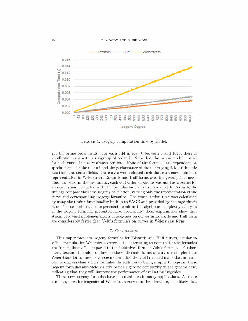
Figure 1. Isogeny computation time by model.

256 bit prime order fields. For each odd integer k between 3 and 1023, there isan elliptic curve with a subgroup of order k. Note that the prime moduli variedfor each curve, but were always 256 bits. None of the formulas are dependant onspecial forms for the moduli and the performance of the underlying field arithmeticwas the same across fields. The curves were selected such that each curve admits arepresentation in Weierstrass, Edwards and Huff forms over the given prime mod-ulus. To perform the the timing, each odd order subgroup was used as a kernel foran isogeny and evaluated with the formulas for the respective models. As such, thetimings compare the same isogeny calcuation, varying only the representation of thecurve and corresponding isogeny formulae. The computation time was calculatedby using the timing functionality built in to SAGE and provided by the sage timeitclass. These performance experiments confirm the algebraic complexity analysesof the isogeny formulas presented here; specifically, these experiments show thatstraight forward implementations of isogenies on curves in Edwards and Huff formare considerably faster than Velu’s formula’s on curves in Weierstrass form.

7. Conclusion

This paper presents isogeny formulas for Edwards and Huff curves, similar toVelu’s formulas for Weierstrass curves. It is interesting to note that these formulasare “multiplicative”, compared to the “additive” form of Velu’s formulas. Further-more, because the addition law on these alternate forms of curves is simpler thanWeierstrass form, these new isogeny formulas also yield rational maps that are sim-pler to express than Velu’s formulas. In addition to being simpler to express, theseisogeny formulas also yield strictly better algebraic complexity in the general case,indicating that they will improve the performance of evaluating isogenies.

These new isogeny formulas have potential uses in many applications. As thereare many uses for isogenies of Weierstrass curves in the literature, it is likely that


the faster evaluation of Edwards (or Huff) isogenies could improve performance ofthese results by switching models. This is similar to how the Edwards addition lawcan speed up point multiplication on elliptic curves. Such possibilities include theSEA algorithm [32], pairings [6], the Doche-Icart-Kohel technique [11], or in publickey cryptosystems [21].

This paper leaves many directions for future work. The preliminary operationcounts show the isogeny formulas are efficient, however this analysis is incompleteand it remains to do a deep optimization of the computations in section 6. Anothersimilar research topic is derivations of similar isogeny formulas for other models ofcurves, such as Hessian curves, Jacobi quartics or Jacobi intersections. Yet anotherinteresting direction would be to address some of the other computational problemsassociated with isogenies (mentioned in the introduction.) In particular the problemof computing an isogeny of known degrees from the domain and codomain.

References

[1] O. Ahmadi, and R. Granger, On isogeny classes of Edwards curves over finite fields, J. NumberTheory, 132 (6), pp. 1337-1358, (2011).

[2] D. Bernstein, P. Birkner, M. Joye, T. Lange, C. Peters. Twisted Edwards curves, in: Progress

in cryptology—AFRICACRYPT 2008, S. Vaudenay (ed.), Lecture Notes in Comput. Sci.5023, Springer, pp. 389–405 (2008).

[3] D. Bernstein, and T. Lange, Faster addition and doubling on elliptic curves, in: Advances

in cryptology—ASIACRYPT 2007, K. Kurosawa (ed.), Lecture Notes in Comput. Sci. 4833,Springer, pp. 29-50 (2007).

[4] G. Bisson, and A. Sutherland, Computing the Endomorphism Ring of an Ordinary Elliptic

Curve over a Finite Field, J. Number Theory, 131 (5), pp. 815–831, (2011).[5] A. Bostan, F. Morain, B. Salvy, and E. Schost, Fast algorithms for computing isogenies

between elliptic curves, Math. Comp. 77, pp. 1755–1778, (2008).[6] R. Broker, D. Charles, and K. Lauter. Evaluating large degree isogenies and applications to

pairing based cryptography, in: Pairing 08: Proceedings of the 2nd international conference

on Pairing-Based Cryptography, Lecture Notes in Comput. Sci. 5209, Springer-Verlag, pp.100-112, (2008).

[7] R. Broker, K. Lauter, and A. Sutherland, Modular polynomials via isogeny volcanoes, Math.

Comp. 81, pp. 1201-1231, (2012).[8] D. Charles, E. Goren, and K. Lauter, Cryptographic hash functions from expander graphs,

J. Cryptology, 22 (1), pp. 93–113, (2009).

[9] H. Debiao, C. Jianhua, and H. Jin, A Random Number Generator Based on Isogenies Opera-tions, Cryptology ePrint Archive Report 2010/94, (2010). Available at http://eprint.iacr.

org/2010/094.

[10] L. De Feo. Algorithmes Rapides pour les Tours de Corps Finis et les Isogenies, PhD thesis.Ecole Polytechnique X, (2010).

[11] C. Doche, T. Icart, and D. Kohel, Efficient Scalar Multiplication by Isogeny Decompositions,in: Public Key Cryptography-PKC 2006, Lecture Notes in Comput. Sci. 3958, Springer-Verlag, pp. 285–352, (2006).

[12] H. Edwards, A normal form for elliptic curves, Bull. Amer. Math. Soc. 44, pp. 393–422 (2007).[13] N. Elkies, Elliptic and modular curves over finite fields and related computational issues, In:

Computational perspectives on number theory: proceedings of a conference in honor of AOLAtkin, D.A. Buell and J.T. Teitelbaum (Eds.), pp. 21–76 (1997).

[14] R. Farashahi, On the Number of Distinct Legendre, Jacobi, Hessian and Edwards Curves(Extended Abstract), in: Proceedings of the Workshop on Coding theory and Cryptology

(WCC 2011), pp. 37–46, (2011). Available at hal.inria.fr/docs/00/60/72/79/PDF/76.pdf.[15] R. Farashahi, D. Moody, and H. Wu, Isomorphism classes of Edwards curves over finite fields,

Finite Fields Appl. (18), pp. 597–612, (2012).

[16] R. Farashahi, I. Shparlinski. On the number of distinct elliptic curves in some families. Des.Codes Cryptogr. 54(1), pp. 83–99, (2010).


[17] R. Feng, and H. Wu, Elliptic curves in Huff’s model, Cryptology ePrint Archive Report

2010/390, (2010). Available at http://eprint.iacr.org/2010/390.pdf.

[18] M. Fouquet, and F. Morain, Isogeny Volcanoes and the SEA Algorithm, In: Proceedings ofthe 5th International Symposium on Algorithmic Number Theory (ANTS-V), C. Fieker and

D. Kohel (Eds.). Springer-Verlag, pp. 276–291, (2002).

[19] L. Hitt, G. Mcguire, and R. Moloney, Division polynomials for twisted Edwards curves,Preprint, (2008). Available at http://arxiv.org/PS_cache/arxiv/pdf/0907/0907.4347v1.

pdf.

[20] G. Huff, Diophantine problems in geometry and elliptic ternary forms, Duke Math. J. 15, pp.443–453, (1948).

[21] D. Jao, and L. de Feo, Towards quantum-resistant cryptosystems from supersingular elliptic

curve isogenies, Post-Quantum Cryptography pp. 19-34 (2011).[22] D. Jao, S. D. Miller, and R. Venkatesan, Do all elliptic curves of the same order have the

same difficulty of discrete log?, In: Advances in Cryptology ASIACRYPT 2005, B. Roy(Ed.), Lecture Notes in Comput. Sci. 3788, pp. 21–40, (2005).

[23] M. Joye, M. Tibouchi, and D. Vergnaud, Huff’s model for elliptic curves, In: 9th Algorithmic

Number Theory Symposium (ANTS-IX), G. Hanrot, F. Morain, E. Thome, (Eds.), LectureNotes in Comput. Sci. 6197, Springer-Verlag, pp. 234–250, (2010).

[24] G. McGuire, and R. Moloney, Two Kinds of Division Polynomials For Twisted Edwards

Curves, Appl. Algebra Engrg. Comm. Comput. 22 (5), pp. 321–345, (2011).[25] D. Kohel, Endomorphism Rings of Elliptic Curves over Finite Fields, PhD thesis, University

of California at Berkeley, (1996).

[26] R. Lercier and F. Morain, Algorithms for computing isogenies between elliptic curves, in:Computational Perspectives on Number Theory, AMS/IP Stud. Adv. Math. 7, Amer. Math.

Soc., pp. 77–96, (1997).

[27] D. Moody, Using 5-isogenies to quintuple points on elliptic curves, Inf. Process. Lett. 111 (7),pp. 314–317, (2011).

[28] A. Rostovtsev and A. Stolbunov, Public-key cryptosystem based on isogenies, CryptologyePrint Archive, Report 2006/145, (2006). Available at http://eprint.iacr.org/2006/145.

[29] SAGE software, Version 4.3.5, http://sagemath.org.

[30] D. Shumow, Isogenies of Elliptic Curves: A Computational Approach, Masters Thesis, Uni-versity of Washington, (2009).

[31] J. Silverman, The arithmetic of elliptic curves, Springer-Verlag, New York, (1986).

[32] R. Schoof, Elliptic curves over finite fields and the computation of square roots mod p, Math.Comp. 44, pp. 483–494, (1985).

[33] A. Stolbunov, Constructing public-key cryptographic schemes based on class group action on

a set of isogenous elliptic curves, Adv. Math. Commun. 4(2), pp. 215–235, (2010).[34] A. Sutherland, Computing Hilbert class polynomials with the Chinese Remainder Theorem,

Math. Comp. 80, pp.501-538, (2011).

[35] E. Teske, An Elliptic curve trapdoor system, J. Cryptology, 19 (1), pp. 115–133, (2006).[36] J. Velu, Isogenies entre courbes elliptiques, C.R. Acad. Sc. Paris, Serie A., 273, pp. 238–241

(1971).[37] L. Washington, Elliptic curves (Number theory and cryptography), 2nd edition, Chapman &

Hall, Boca Raton, Fl, (2008).

Computer Security Division, National Institute of Standards and Technology (NIST),

Gaithersburg MD, USAE-mail address: [email protected]

eXtreme Computing Group, Microsoft Research, Redmond WA, USAE-mail address: [email protected]

analogues of velu’s formulas for …analogues of velu’s formulas for isogenies 3 2....

Documents