analisi di protocolli harq per il sistema cellulare ltetesi.cab.unipd.it/46116/1/tesi.pdf · figure...
TRANSCRIPT

Universita degli Studi di PadovaDipartimento di Ingegneria dell’InformazioneCorso di Laurea Magistrale in Ingegneria delleTelecomunicazioni
Tesi di laurea magistrale
Analisi di protocolli HARQper il sistema cellulare LTE
Analysis of HARQ protocolsfor LTE cellular system
Candidato:Marco CentenaroMatricola 1043634
Relatore:Chiar.mo Prof. Lorenzo Vangelista
Anno Accademico 2013–2014

Marco Centenaro: Analysis of HARQ protocols for LTE cellular system, Tesi dilaurea magistrale, c© luglio 2014.
Author’s note.This document was typeset using the LATEX typographical style classicthesisdeveloped by André Miede. This style was inspired by Robert Bringhurst’sseminal book on typography The Elements of Typographic Style [1992].classicthesis is available on ctan (http://www.ctan.org).
Made on a Mac.
Final Version as of July 7, 2014 (classicthesis).

Non quia difficilia sunt non audemus, sed quia non audemus difficilia sunt.
— Lucius Annaeus Seneca
Coloro che s’innamorano di pratica senza scienza sono come nocchiero cheentra in nave senza timone o bussola, che mai ha certezza dove va.
— Leonardo da Vinci


C O N T E N T S1 introduction 1
1.1 A brief introduction to LTE 1
1.2 Network architecture 1
1.3 Protocol stack 2
1.4 Types of channels 2
1.5 OFDM, OFDMA and SC-FDMA 3
1.6 Duplex schemes 4
1.7 Time-frequency resources and scheduling 4
1.8 The LTE MAC layer 5
1.9 Downlink HARQ and Uplink HARQ 6
1.10 Beyond LTE 6
1.11 How to apply intelligence? 6
2 state of the art 9
2.1 What is HARQ? 9
2.2 Block scheme 9
2.3 Turbo coding 10
2.4 Modulation and rate matching 11
2.4.1 Circular buffer 11
2.4.2 Bit selection 11
2.4.3 Digital modulation 13
2.5 Antenna mapping and OFDM modulator 14
2.6 Accumulated Mutual Information 15
2.6.1 Shannon’s coding theorem 15
2.6.2 What is Accumulated Mutual Information? 15
2.6.3 Variable-rate Incremental Redundancy 16
2.7 Notation disclaimer 17
3 proposed solution 19
3.1 Assumptions and parameters 19
3.2 Wireless channel model 20
3.3 CQI model 21
3.4 Channel transitions model 23
3.5 Rate matching process model 25
3.6 Enhanced rate characterization 26
3.7 How to model the accumulated mutual information in LTE? 27
3.8 Markov chain 29
3.8.1 Structure of the chain 29
3.8.2 Rewards 29
3.9 The Bayesian approach 30
4 performance evaluation 31
4.1 Simulation procedure 31
4.1.1 Possible enhancements 32
4.2 Observations 32
4.2.1 Trends 32
4.2.2 Comparison with real simulators 32
4.2.3 Enhancement of the model: does it work? 32
v

vi contents
5 conclusion and future work 39
a channel transition matrix 43
b rate matching modeling and acmi 45
b.1 Rate matching #1 45
b.2 Rate matching #2 46
b.3 Rate matching #3 47
b.4 Rate matching #4 48
b.5 Rate matching #5 49
b.6 Rate matching #6 51
b.7 Rate matching #7 52
c markov chain graph 55
bibliography 57
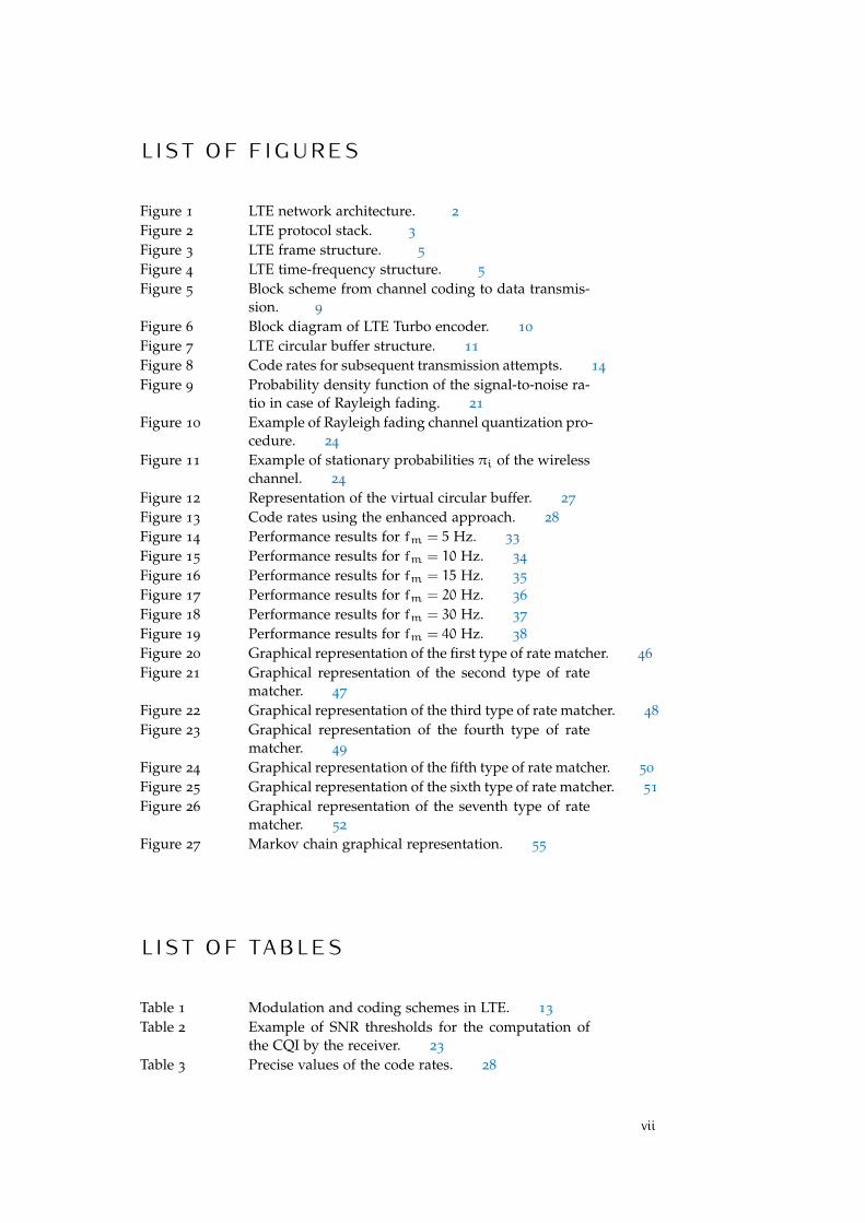
L I S T O F F I G U R E SFigure 1 LTE network architecture. 2
Figure 2 LTE protocol stack. 3
Figure 3 LTE frame structure. 5
Figure 4 LTE time-frequency structure. 5
Figure 5 Block scheme from channel coding to data transmis-sion. 9
Figure 6 Block diagram of LTE Turbo encoder. 10
Figure 7 LTE circular buffer structure. 11
Figure 8 Code rates for subsequent transmission attempts. 14
Figure 9 Probability density function of the signal-to-noise ra-tio in case of Rayleigh fading. 21
Figure 10 Example of Rayleigh fading channel quantization pro-cedure. 24
Figure 11 Example of stationary probabilities πi of the wirelesschannel. 24
Figure 12 Representation of the virtual circular buffer. 27
Figure 13 Code rates using the enhanced approach. 28
Figure 14 Performance results for fm = 5 Hz. 33
Figure 15 Performance results for fm = 10 Hz. 34
Figure 16 Performance results for fm = 15 Hz. 35
Figure 17 Performance results for fm = 20 Hz. 36
Figure 18 Performance results for fm = 30 Hz. 37
Figure 19 Performance results for fm = 40 Hz. 38
Figure 20 Graphical representation of the first type of rate matcher. 46
Figure 21 Graphical representation of the second type of ratematcher. 47
Figure 22 Graphical representation of the third type of rate matcher. 48
Figure 23 Graphical representation of the fourth type of ratematcher. 49
Figure 24 Graphical representation of the fifth type of rate matcher. 50
Figure 25 Graphical representation of the sixth type of rate matcher. 51
Figure 26 Graphical representation of the seventh type of ratematcher. 52
Figure 27 Markov chain graphical representation. 55
L I S T O F TA B L E STable 1 Modulation and coding schemes in LTE. 13
Table 2 Example of SNR thresholds for the computation ofthe CQI by the receiver. 23
Table 3 Precise values of the code rates. 28
vii

viii List of Tables
Table 4 Simulation parameters. 31
L I S T O F A C R O N Y M SACMI ACcumulated Mutual Information
ARQ Automatic Repeat reQuest
AWGN Additive White Gaussian Noise
CC Chase Combining
CC-HARQ Chase Combining Hybrid Automatic Repeat reQuest
CQI Channel Quality Indicator
DCI Downlink Control Information
DFT Discrete Fourier Transform
eNB Evolved NodeB
EPC Evolved Packet Core
EPS Evolved Packet System
e-UTRAN Evolved Universal Terrestrial Radio Access Network
FDD Frequency Division Duplex
FEC Forward Error Correction
GSM Global System for Mobile communications
HARQ Hybrid Automatic Repeat reQuest
IP Internet Protocol
IR Incremental Redundancy
IR-HARQ Incremental Redundancy Hybrid Automatic Repeat reQuest
OFDM Orthogonal Frequency Division Multiplexing
OFDMA Orthogonal Frequency Division Multiple Access
Layer 1 Physical Layer
LL Link Layer
LTE Long Term Evolution
MAC Medium Access Control
MCS Modulation and Coding Scheme
MIMO Multi-Input Multi-Output
MRC Maximum Ratio Combining

List of Tables ix
NAS Non-Access Stratum
OFDM Orthogonal Frequency Division Multiplexing
PAPR Peak-to-Average Power Ratio
PDCP Packet Data Convergence Protocol
PDU Protocol Data Unit
QoS Quality of Service
QPP Quadratic Permutation Polynomial
RB Resource Block
RE Resource Element
RLC Radio Link Control
RRC Radio Resource Control
RV Redundancy Version
SC-FDMA Single-Carrier Frequency Division Multiple Access
SDU Service Data Unit
SNR Signal to Noise Ratio
SINR Signal to Interference plus Noise Ratio
SISO Single-Input Single-Output
SW Stop-and-wait
SW-ARQ Stop and Wait Automatic Repeat reQuest
TB Transport Block
TDD Time Division Duplex
TM Transmission Mode
TTI Transmission Time Interval
UCI Uplink Control Information
UE User Equipment
UMTS Universal Mobile Telecommunications System


S O M M A R I OIn questa tesi vengono studiati i protocolli di Hybrid-Automatic Repeat
reQuest (HARQ) implementati nel sistema cellulare Long Term Evolution(LTE). Vengono ricavati modelli analitici dei suddetti protocolli e viene pro-posta una modifica che, utilizzando un approccio di tipo Bayesiano, nemigliora le prestazioni sia in termini di throughput che di ritardo. La quan-tificazione dei miglioramenti viene effettuata valutando i modelli propostiper via numerica. Il lavoro è stato ispirato dai requisiti delle reti cellulari 5Gche sono in fase di definizione.
A B S T R A C TThe aim of this thesis is studying the Hybrid-Automatic Repeat reQuest
(HARQ) protocols that are implemented in the Long Term Evolution (LTE)cellular system. Analytical models of these processes are derived and anenhancement is proposed in order to increase the throughput and decreasethe delivery delay, exploiting a Bayesian approach. A numerical evaluationof the performances has been carried out. The requirements for 5G networksare the main motivation for this work.
xi


La forza di volontà attraversa anche le rocce.
— Proverbio giapponese
R I N G R A Z I A M E N T IQuesto traguardo non sarebbe mai stato raggiungibile se non avessi avu-
to al mio fianco a sostenermi delle persone veramente speciali. Ringrazio,perciò, con tanto affetto i miei genitori, il mio grande fratello Stefano, nonnie zii, per tutto quello che hanno fatto per me. Inoltre un grande ringra-ziamento va ai miei amici e a Marika, per aver condiviso con me momentiindimenticabili.
Grazie a tutti, di cuore.
Padova, luglio 2014 M. C.
xiii

S T R U T T U R A D E L L A T E S IIl presente elaborato è strutturato in 4 capitoli.
il primo capitolo offre una breve introduzione sulla tecnologia del LongTerm Evolution (LTE) e un primo accenno su come applicare un ap-proccio bayesiano nel processo di trasmissione a livello link layer (LL).
il secondo capitolo fornisce una panoramica sullo stato dell’arte relati-vo allo studio di processi di Hybrid Automatic Repeat reQuest (HARQ).
il terzo capitolo descrive come elaborare un modello del processo diHARQ e come sfruttarlo per valutare l’incremento delle prestazioniapplicando l’approccio bayesiano.
il quarto capitolo contiene i risultati numerici e i grafici relativi alleprestazioni del sistema.
xv


1 I N T R O D U C T I O N
1.1 a brief introduction to lteLong Term Evolution (LTE) is a standard for cellular wireless communi-
cation of high-speed data for mobile phones and data terminals. It is basedon the Global System for Mobile communications (GSM) and Universal Mo-bile Telecommunications System (UMTS) network technologies, increasingcapacity and speed using a different radio interface together with core net-work improvements. As its predecessors, this standard is developed by the3GPP association (3rd Generation Partnership Project)1.
LTE or the Evolved Universal Terrestrial Radio Access Network (e-UTRAN)is the access part of the Evolved Packet System (EPS), which is purely In-ternet Protocol (IP) based. This new access solution is based on OrthogonalFrequency Division Multiple Access (OFDMA). In combination with higherorder modulation (up to 64-QAM), large bandwidths (up to 20 MHz) andspatial multiplexing in the downlink (up to 4× 4-MIMO) high data rates canbe achieved. The highest theoretical peak data rate on the transport channelis 75 Mbps in the uplink and up to 300 Mbps in the downlink.
To enable possible deployment around the world, supporting as manyregulatory requirements as possible, LTE is developed for a number of fre-quency bands currently ranging from 700MHz up to 2.7 GHz. The availablebandwidths are also flexible, starting with 1.4 MHz up to 20 MHz.
1.2 network architectureThe network architecture of LTE (also known as EPS) consists of three
main components:
• the User Equipment (UE). The internal architecture of the UE for LTEis identical to the one used by UMTS and GSM which is actually aMobile Equipment.
• the e-UTRAN (access network). The e-UTRAN handles the radio com-munications between the mobile and the core network and has justone component: the Evolved NodeB (eNB). Each eNB is a base stationthat controls the mobiles in one or more cells; the base station that iscommunicating with a mobile is known as its serving eNB. Each eNBconnects with the EPC by means of the S1 interface and it can alsobe connected to nearby base stations by the X2 interface to performsignaling and packet forwarding during handover.
• the Evolved Packet Core (EPC). It represents the core network of thesystem, performing switching, authentication and connection to otherpacket (IP) networks and telephone networks.
A graphical representation of the LTE network architecture is shown inFigure 1.
1 http://www.3gpp.org, last visited July 7, 2014
1

2 introduction
Figure 1: LTE network architecture.
1.3 protocol stackThe LTE protocol stack is organized as follows:
• the Physical Layer (Layer 1) carries all information from the MACtransport channels (see 1.4) over the air interface.
• the Medium Access Control (MAC) is responsible for mapping be-tween logical channels and transport channels (see 1.4), multiplex-ing/demultiplexing MAC Service Data Units (SDUs) from logical chan-nels into Transport Blocks (TBs) to be delivered to/delivered by theLayer 1 on transport channels, error correction through HARQ (see1.8).
• the Radio Link Control (RLC) is responsible for transfer of upper layerProtocol Data Units (PDUs), error correction through Automatic Re-peat reQuest (ARQ), concatenation, segmentation and reassembly ofRLC SDUs.
• the Radio Resource Control (RRC) provides services such as broad-cast of system information, paging, establishment, maintenance andrelease of an RRC connection between the UE and e-UTRAN, security.
• the Packet Data Convergence Protocol (PDCP) is responsible for headercompression/decompression of IP data, in-sequence delivery of upperlayer PDUs, duplicate discarding.
• the Non-Access Stratum (NAS) supports the mobility of the UE andthe session management procedures to establish and maintain IP con-nectivity.
A graphical representation of it is shown in Figure 2.
1.4 types of channelsIn LTE three categories of channels are defined:

1.5 ofdm, ofdma and sc-fdma 3
logical channels These channels define what type of information is trans-mitted over the wireless channel, either data or control messages. TheMAC provides services to the RLC in the form of logical channels.
transport channels They define how and with what characteristics the in-formation is transmitted over the radio interface. The MAC layer usesservices from the Layer 1 in the form of transport channels.
physical channels They correspond to sets of time-frequency resources(see 1.7) used for transmission of a particular transport channel. Eachtransport channel is mapped to a corresponding physical channel,but there are also physical channels without a corresponding trans-port channel: these channels are used for Downlink Control Informa-tion (DCI), providing the terminal with the necessary information forproper reception and decoding of the downlink data transmission, andUplink Control Information (UCI) used for providing the schedulerand the Hybrid Automatic Repeat reQuest (HARQ) protocol with in-formation about the situation at the terminal.
Figure 2: LTE protocol stack.
1.5 ofdm, ofdma and sc-fdmaTo overcome the effect of multipath fading, LTE uses Orthogonal Fre-
quency Division Multiplexing (OFDM) for the downlink, exploiting a largenumber of narrow subcarriers for multi-carrier transmission to carry data in-stead of spreading one signal over the entire bandwidth. In OFDMA thesesubcarriers can be shared between multiple users. The OFDMA solutionleads to high Peak-to-Average Power Ratios (PAPRs), requiring expensivepower amplifiers with hard requirements on linearity and, therefore, increas-ing the power consumption for the transmitter. This is not a problem if thetransmitter is the eNB, i.e, in the downlink, but it becomes a problem if thetransmitter is the UE. Hence a different solution has been designed for theuplink: the Single-Carrier Frequency Division Multiple Access (SC-FDMA)solution generates a signal with single carrier characteristics, i.e., with a lowPAPR, by grouping together the resource blocks (see 1.7).

4 introduction
1.6 duplex schemesLTE is developed to support both the Frequency Division Duplex (FDD)
and the Time Division Duplex (TDD). In FDD uplink and downlink trans-missions use disjoint frequency bands, whereas in TDD they share the samecarrier but are separated in time. In TDD and FDD up to 15 and 8 HARQprocess are considered in parallel, respectively.
1.7 time-frequency resources and schedul-ing
LTE considers a slotted time axis in which:
• one frame lasts Tframe = 10 ms;
• each frame is composed of 10 subframes of duration Tsubframe = 1 ms;
• every subframe is divided into 2 time slots of duration Tslot = 0.5 ms;
• every slot contains 7 OFDM symbols: Tsymbol = 0.067 ms2.
• every OFDM symbol contains up to 2048 OFDM samples: Ts = 0.325ns.
Considering Ts as the basic time unit, we can express the other quantities infunction of it as:
Tsymbol = 2048 · TsTslot = 15360 · Ts
Tsubframe = 30720 · TsTframe = 307200 · Ts
The subframe duration is also denoted as Transmission Time Interval (TTI):
Tsubframe = TTI
For what concerns the frequency bands, instead, many possibilities interms of carrier frequency fc and bandwidth B are available. In every case,the total band is split into sub-bands of 180 kHz bandwidth, each one con-taining 12 subcarriers spaced of 15 kHz. We call Resource Block (RB) thetime-frequency unit of 0.5 ms times 180 kHz and Resource Element (RE)the time-frequency unit of one OFDM symbol times one subcarrier. Thus,each RB consists of 7 · 12 = 84 REs. In LTE the time-frequency resources areshared between users and they are dynamically assigned by the schedulerin terms of resource-block pairs, i.e., couples of RB (time-frequency units of1 ms times 180 kHz).
Figure 3 may explain better the structure of the time axis; Figure 4, instead,shows the time-frequency grid structure in LTE.
2 Tsymbol < Tslot/7 because we must account for the cyclic prefix.

1.8 the lte mac layer 5
Figure 3: LTE frame structure.
Figure 4: LTE time-frequency structure.
1.8 the lte mac layerAll Layer 1 transport data are encoded using a turbo code with a Quadratic
Permutation Polynomial (QPP) internal interleaver. We recall that a permu-tation polynomial, for a given ring, is a polynomial that acts as a permuta-tion of the elements of the ring; it is quadratic if the polynomial is of degreetwo. Since the receiver is capable of asking for a retransmission of the packetin case of decoding failures, an ARQ retransmission process is employed ontop of the Forward Error Correction (FEC) turbo code, establishing an over-all Hybrid Automatic Repeat reQuest (HARQ) process. The applied ARQprocess is a Stop and Wait Automatic Repeat reQuest (SW-ARQ) one.
The coding rate of the mother turbo code is
Rc =1
3
however many other coding schemes are available thanks to puncturingpatterns provided in the rate matching process after the encoding block. Thepatterns are selected according to the Channel Quality Indicator (CQI) index.The CQI is a parameter that indicates the state of the channel (whether it isgood or bad), using a scale of 15 values; this piece of information is reportedto the source by the destination, together with the acknowledgment/not-acknowledgement of the previously transmitted packet. The type of digitalmodulation is selected depending on the CQI value, so the modulation inLTE is adaptive.

6 introduction
1.9 downlink harq and uplink harqA HARQ process in LTE can be
• synchronous: the retransmissions take place after a constant period oftime
• asynchronous: the retransmissions can take place whenever in time,due to scheduling purposes. In this cases we need an appropriatesignaling to make the transmitter aware of which HARQ process weare considering.
We can distinguish also between other two kinds of HARQ process:
• adaptive: the transmission parameters (including the Redundancy Ver-sion, see 2.4.1) are decided on the fly by the scheduler
• non-adaptive: the transmission parameters are those that have beendefined at the first transmission attempt and they don’t change. In thiscase subsequent retransmissions take progressive Redundancy Versionindexes.
Depending on the direction of the transmission, in LTE we have that
• the downlink HARQ is asynchronous and adaptive
• the uplink HARQ is synchronous and non-adaptive.
1.10 beyond lteRecent studies and extrapolations from past developments predict a total
traffic increase by a factor of 500 to 1000 within the next decade. Thesefigures assume approximately a 10 times increase in broadband mobile sub-scribers, and 50-100 times higher traffic per user. Besides the overall traffic,the achievable throughput per user has to be increased significantly. A rough esti-mation predicts a minimum 10 times increase in average, as well as in peak,data rate.
Moreover, essential design criteria, which have to be fulfilled more effi-ciently than in today’s systems, are fairness between users over the wholecoverage area, latency to reduce response time and better support for a mul-titude of Quality of Service (QoS) requirements originating from differentservices3.
1.11 how to apply intelligence?In the LTE uplink, which is synchronous and non-adaptive, the Modula-
tion and Coding Scheme (MCS) is determined by the last CQI index that thesource reads in the feedback packet sent by the destination. However, thisapproach may let us experience inefficiencies in some cases, e.g. in case ofdeep fading events, in which the transmitter employs the most resilient MCSfor the next transmission attempt even though the channel becomes good
3 http://www.networks-etp.eu/fileadmin/user_upload/Home/draft-PPP-proposal.pdf, lastvisited July 7, 2014

1.11 how to apply intelligence? 7
again, yielding an inherent throughput reduction. On the opposite side, ifwe experience a very favourable (but instantaneous) condition for the chan-nel then we may employ a too optimistic MCS, causing a sequence of failedtransmissions and yielding again to a throughput reduction.
We would like to propose a Bayesian approach, in which the network
1. observes how the channel changes over time, storing data in a cognitiverepository,
2. learns from the gathered data,
3. plans the action, trying to predict the future behaviour of the channeland finally
4. acts, tuning the MCS appropriately in order to increase the throughputof the system.

2 S TAT E O F T H E A R T
2.1 what is harq?In Chapter 1 we mentioned that LTE MAC layer employs jointly a FEC
turbo coding approach and a SW-ARQ retransmission process, i.e., a HARQprocess. According to the literature, two kinds of HARQ processes are usu-ally considered, depending on how the receiver treats the erroneously re-ceived packets:
harq-type i After each transmission attempt the received packet is dis-carded if it is erroneous.
harq-type ii After each transmission attempt the received packet, if erro-neous, is stored in a buffer and then combined with subsequent trans-mitted packets, in order to increase the performances of the FEC code.We can make a further distinction between the following two sub-categories of HARQ-II processes, depending on how the receiver com-bines the multiple versions of the erroneously received packets:
cc-harq If the transmission involves always the same packet in dif-ferent attempts then we have a Chase Combining Hybrid Auto-matic Repeat reQuest (CC-HARQ); at the receiver side a Maxi-mum Ratio Combining (MRC) of the received replicas is appliedin order to improve resiliance to noise and, therefore, the FECperformances.
ir-harq In Incremental Redundancy Hybrid Automatic Repeat re-Quest (IR-HARQ), instead, the transmitter splits the entire codedmessage in sub-codewords that are sent in subsequent transmis-sion attempts; the receiver combines them appropriately.
We will see in the next sections that LTE follows a mixed approach, usingboth CC-HARQ and IR-HARQ.
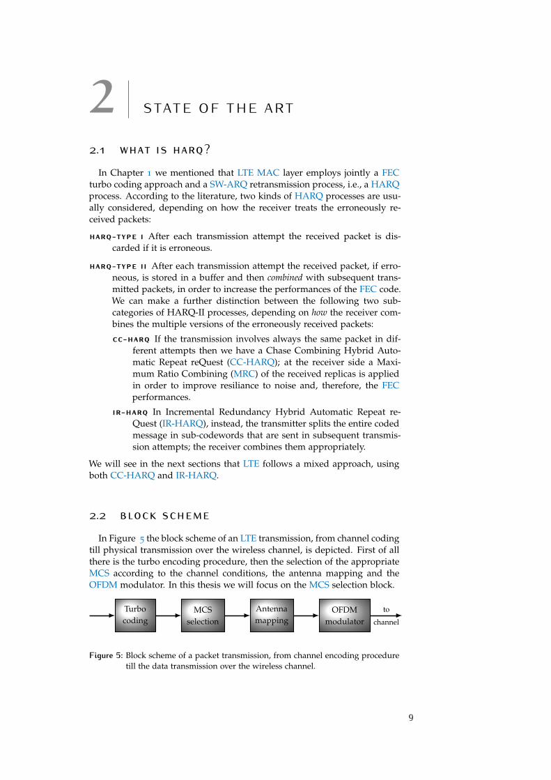
2.2 block schemeIn Figure 5 the block scheme of an LTE transmission, from channel coding
till physical transmission over the wireless channel, is depicted. First of allthere is the turbo encoding procedure, then the selection of the appropriateMCS according to the channel conditions, the antenna mapping and theOFDM modulator. In this thesis we will focus on the MCS selection block.
Turbocoding
MCSselection
Antennamapping
OFDMmodulator
to
channel
Figure 5: Block scheme of a packet transmission, from channel encoding proceduretill the data transmission over the wireless channel.
9

10 state of the art
2.3 turbo codingThe FEC part of the HARQ framework is performed by a turbo code of
mother code rateRc =
1
3
The encoding process consists of two rational, rate-1/2 constituent encoderswith generating vector
g(D) =
[1
1+D+D3
1+D2+D3
]in combination with QPP interleaving, which provides a mapping from theinput (non-interleaved) bits to the output (interleaved) bits according to thefunction
Π(i) =(f1i+ f2i
2)
mod K
where
• i is the index of the input bit in the original sequence
• Π(i) is the index of the same bit in the interleaved sequence
• K is the block length
• f1 and f2 are parameters that depend on the value of K.
Figure 6: Block diagram of LTE Turbo encoder.
In Figure 6 the block diagram of LTE Turbo encoder is depicted. It canseen that the encoding procedure produces three bit streams:
1. the first stream contains the unprocessed input bits, i.e. the systematicbits
2. the second stream is the one that carries the parity bit produced by thefirst constituent encoder, i.e. the first parity bits
3. the third stream carries the parity bits generated by the second con-stituent encoder, i.e. the second parity bits.
Therefore, this turbo code is systematic since the input data is embedded inthe first part of the encoded output sequence.

2.4 modulation and rate matching 11
2.4 modulation and rate matching2.4.1 Circular buffer
The three output streams of the Turbo encoder experience a row-columninterleaving separately and they are inserted in a circular buffer (see Figure 7)where the systematic bits fill the first positions, followed by alternating in-sertions of the first and second parity bits (interlacing procedure). A subsetof consecutive bits called Redundancy Version (RV) is then extracted fromthe circular buffer; the size of this subset is such that it matches the num-ber of avaliable resource elements in the resource blocks assigned for thetransmission. The exact set of extracted bits depend on the RV index, cor-responding to different starting points for the extraction of coded bits fromthe circular buffer. There are four alternatives for the RV, as many as theallowed transmission attempts. The selection of the appropriate subset ofbits is done by the bit selection block.
Figure 7: LTE circular buffer structure: we can distinguish the systematic bits block(from 0 to X = number of systematic bits) and the interlaced parity bitsblock (from X to 3X). Note also the four starting points for the extractionsof the bits for the different RVs.
2.4.2 Bit selectionThe puncturing patterns for the RV bit selection depend on the value of
the CQI, which is the numerical index that indicates how good the channelis. In LTE there exist N = 15 values for the CQI (integer values belongingto the set {1, . . . , 15}), each one corresponding to a particular MCS that isrequired for the next packet transmission. In literature [Kwan and Ikuno,2013] we can find methods to analitically characterize the code rate we ob-tain after the n-th transmission attempt, using a combination of an innerchannel code processing unrepeated bits with a code rate of R(n)c and anouter repetition code with rate 1/Nn working on the output of the preced-ing channel code.
12 state of the art
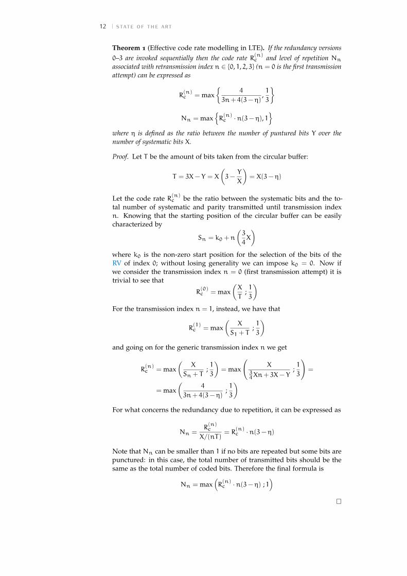
Theorem 1 (Effective code rate modelling in LTE). If the redundancy versions0–3 are invoked sequentially then the code rate R(n)c and level of repetition Nnassociated with retransmission index n ∈ {0, 1, 2, 3} (n = 0 is the first transmissionattempt) can be expressed as
R(n)c = max
{4
3n+ 4(3− η),1
3
}
Nn = max{R(n)c ·n(3− η), 1
}where η is defined as the ratio between the number of puntured bits Y over thenumber of systematic bits X.
Proof. Let T be the amount of bits taken from the circular buffer:
T = 3X− Y = X
(3−
Y
X
)= X(3− η)
Let the code rate R(n)c be the ratio between the systematic bits and the to-tal number of systematic and parity transmitted until transmission indexn. Knowing that the starting position of the circular buffer can be easilycharacterized by
Sn = k0 +n
(3
4X
)where k0 is the non-zero start position for the selection of the bits of theRV of index 0; without losing generality we can impose k0 = 0. Now ifwe consider the transmission index n = 0 (first transmission attempt) it istrivial to see that
R(0)c = max
(X
T;1
3
)For the transmission index n = 1, instead, we have that
R(1)c = max
(X
S1 + T;1
3
)and going on for the generic transmission index n we get
R(n)c = max
(X
Sn + T;1
3
)= max
(X
34Xn+ 3X− Y
;1
3
)=
= max(
4
3n+ 4(3− η);1
3
)For what concerns the redundancy due to repetition, it can be expressed as
Nn =R(n)c
X/(nT)= R
(n)c ·n(3− η)
Note that Nn can be smaller than 1 if no bits are repeated but some bits arepunctured: in this case, the total number of transmitted bits should be thesame as the total number of coded bits. Therefore the final formula is
Nn = max(R(n)c ·n(3− η) ; 1
)

2.4 modulation and rate matching 13
Please note that, as it is defined, R(n)c is not the coding rate of the retrans-mission of index n, but the effective code rate after the n-th retransmission(without considering the repeated bits, i.e., considering the saturation of therate to the mother code rate of 1/3 in those cases in which Sn + T exceedsthe size of the circular buffer).
The modulation and coding schemes which are available in LTE are shownin Table 1. In the same Table the values of η for all the CQI indexes can befound; these values have been computed inverting the previous expression:
R(0)c,REP =
4
3 · 0+ 4(3− η)=
1
3− η⇒ η = 3−
1
R(0)c,REP
where the values of R(0)c,REP can be found in Ikuno et al., 2011. The availablecode rates for the different RVs are shown in Figure 8.
Table 1: Modulation and coding schemes in LTE. R(0)c and R(0)c,REP indicate the coderate of the first transmission attempt without considering the repeated bitsand considering them, respectively.
CQI k Modulation η R(0)c R
(0)c,REP
1 QPSK −10.1300 1/3 0.0762 QPSK −5.5300 1/3 0.123 QPSK −2.3100 1/3 0.194 QPSK −0.3200 1/3 0.305 QPSK 0.7200 0.44 0.446 QPSK 1.3000 0.59 0.59
7 16-QAM 0.2900 0.37 0.378 16-QAM 0.9100 0.48 0.489 16-QAM 1.3400 0.60 0.60
10 64-QAM 0.8000 0.45 0.4511 64-QAM 1.1900 0.55 0.5512 64-QAM 1.4600 0.65 0.6513 64-QAM 1.6700 0.75 0.7514 64-QAM 1.8300 0.85 0.8515 64-QAM 1.9200 0.93 0.93
2.4.3 Digital modulationThe block of bits delivered by the HARQ functionality is then multiplied
(exclusive-OR operation) by a bit-level scrambling sequence and the map-ping to complex modulation symbols is finally performed according to oneof the following digital modulation schemes:
1. QPSK
2. 16-QAM
3. 64-QAM
corresponding to two, four or six bits per symbol, respectively.
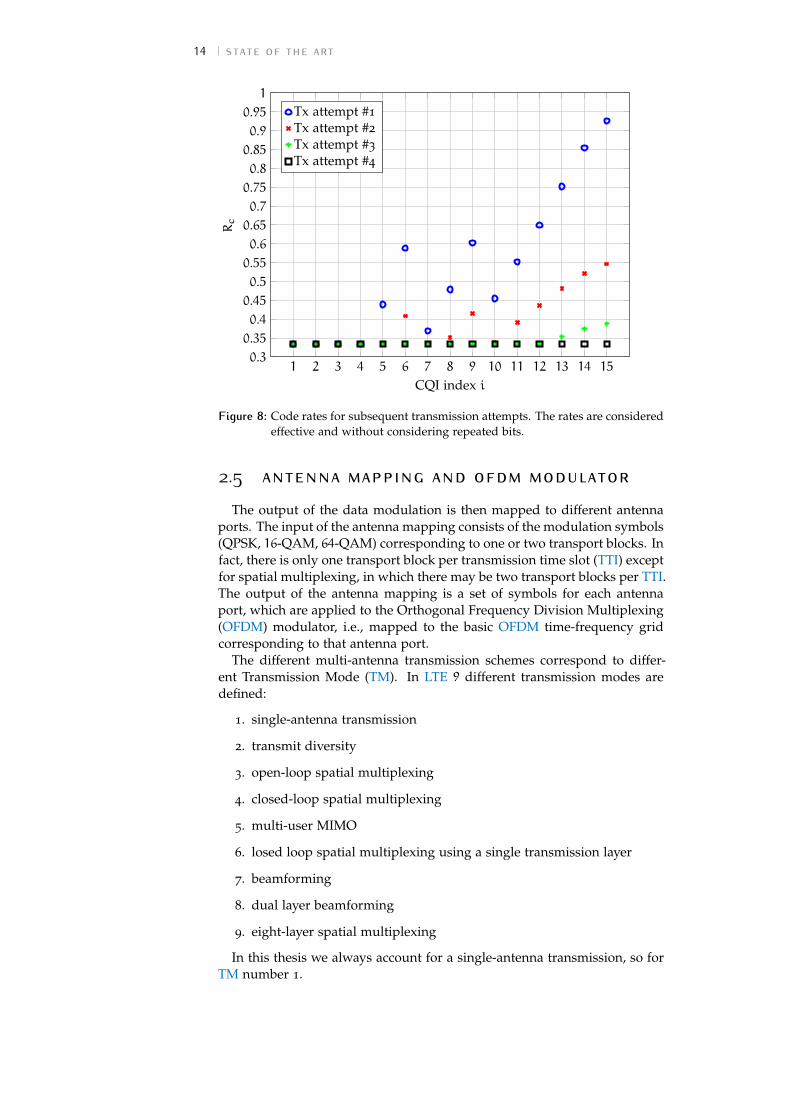
14 state of the art
1 2 3 4 5 6 7 8 9 10 11 12 13 14 150.30.350.40.450.50.550.60.650.70.750.80.850.90.951
CQI index i
Rc
Tx attempt #1
Tx attempt #2
Tx attempt #3
Tx attempt #4
Figure 8: Code rates for subsequent transmission attempts. The rates are consideredeffective and without considering repeated bits.
2.5 antenna mapping and ofdm modulatorThe output of the data modulation is then mapped to different antenna
ports. The input of the antenna mapping consists of the modulation symbols(QPSK, 16-QAM, 64-QAM) corresponding to one or two transport blocks. Infact, there is only one transport block per transmission time slot (TTI) exceptfor spatial multiplexing, in which there may be two transport blocks per TTI.The output of the antenna mapping is a set of symbols for each antennaport, which are applied to the Orthogonal Frequency Division Multiplexing(OFDM) modulator, i.e., mapped to the basic OFDM time-frequency gridcorresponding to that antenna port.
The different multi-antenna transmission schemes correspond to differ-ent Transmission Mode (TM). In LTE 9 different transmission modes aredefined:
1. single-antenna transmission
2. transmit diversity
3. open-loop spatial multiplexing
4. closed-loop spatial multiplexing
5. multi-user MIMO
6. losed loop spatial multiplexing using a single transmission layer
7. beamforming
8. dual layer beamforming
9. eight-layer spatial multiplexing
In this thesis we always account for a single-antenna transmission, so forTM number 1.

2.6 accumulated mutual information 15
2.6 accumulated mutual information2.6.1 Shannon’s coding theorem
A very important tool for the study of HARQ processes is the ACcumu-lated Mutual Information (ACMI). We first need to recall one of the funda-mental theorems of information theory: the Shannon theorem on channelcoding.
Theorem 2 (Shannon’s channel coding theorem). Let us define the informa-tion rate
R∆=
log2Mn
[bit/channel use]
where M is the cardinality of the symbol alphabet and n the size of the codewordsat the input of the channel, and the capacity of the channel
C∆= max I(x;y)
where I(x;y) is the mutual information between the input and the output of thechannel. Then, for rates R < C and n sufficiently large there is an encoder/decoderprocedure assuring a symbol error probability Pe as small as desired, i.e. to en-sure reliable communications. If, instead, R > C a reliable communication is notpossible.
Note that the information rate can be equivalently expressed in the fol-lowing way
R =log2Mn
= Rc · log2M [bit/channel use]
recalling that Rc is the code rate of the transmitted message and M is thecardinality of the set of symbols, which depends on the type of modulationscheme that is applied.
2.6.2 What is Accumulated Mutual Information?After having recalled the Shannon theorem, we can define the ACMI I?(γ)
straighforward: it is a way of increasing the capacity of the channel througha retransmission process.
setting Let x be a codeword of fixed length N bits, produced by an inputsequence u of Nb bits; divide it in B sub-codewords x = (x1, . . . , xB) of
lengths Ns∆= N/B. Thus each subcodeword may be seen as a result of a
coding procedure with rate
Rc =NbNs
=NbN/B
= B · NbN
where Nb/N is the code rate of the original codeword x.
definition of accumulated mutual information Depending on thekind of HARQ-type II employed, we provide a different definition for theACMI I?(γ), depending on the type of HARQ:
• In the case of CC-HARQ, we are increasing the resilience to channelnoise so
ICC? (γ)
∆= C
(m∑i=1
γi
)

16 state of the art
• For IR-HARQ, instead, we are sending adding redundancy at everytransmission attempt so
IIR? (γ)∆=
m∑i=1
C(γi)
where m is the index of the last transmission attempt carried out.In particular, the expression provided for the incremental redundancy
approach is designed for a parity priority IR-HARQ. It is the most commonincremental redundancy approach: at every transmission attempt one sub-codeword from the entire original one is sent over the channel. However, insystematic codes, to ensure that every transmitted packet is self-decodable,each RV consists of the information bits and some new redundancy bits:
Ns = Nb +Nr
where Nr = (N−Nb)/B is the fixed amount of new redundancy bits thatis employed in every transmitted packet. At the receiver side the informa-tion part of the message is combined with its previously received versions,whereas the redundancy bits decrease the coding rate: in other words, thefirst ones experience a CC-HARQ and the second ones a IR-HARQ. Thisis the reasoning that stands behind the expression for the systematic priorityACMI:
IIR,SP? (γ)
∆= Rc ·C
(m∑i=1
γi
)+ (1− Rc) ·
m∑i=1
C(γi)
whereRc =
NbNb +Nr
is the constant coding rate of each transmission.In any case, the condition for ensuring reliable communications given by
the Shannon’s theorem then becomes
I?(γ) < R = Rc · log2M = [M = 2] = Rc
See Caire and Tuninetti, 2001 for more details.
2.6.3 Variable-rate Incremental RedundancyIn the previous calculations, we have been assuming that the coding rate
of each transmitted subcodeword is constant:
Rc =NbNs
= const < 1
However we can generalize the definition of ACMI in the case of a variable-rate IR-HARQ process (see Szczecinski et al., 2010). Consider that each sub-codeword has a different length of Ns,i symbols of an alphabet of size M;then we have that
I?(γ) =1∑m
i=1Ns,i
m∑i=1
C(γi)Ns,i
The condition from the Shannon theorem to provide a reliable communi-cation becomes
I?(γ) <Nb∑mi=1Ns,i
· log2M

2.7 notation disclaimer 17
or in an equivalent way
m∑i=1
C(γi)Ns,i
Nb=
m∑i=1
C(γi)
Rc,i< log2M
where Rc,i is the coding rate of the i-th transmitted packet.Note that, in case we have Ns,i = Ns,j ∀i, j, it follows that Rc,i = Rc and
so we have
I?(γ) =
m∑i=1
C(γi)
and the condition of Shannon’s channel coding theorem is the same weintroduced at the beginning
I?(γ) =
m∑i=1
C(γi) < Rc · log2M
2.7 notation disclaimerNote the differences in the notation in the following cases:
• code rateRc =
NbNs
It is the constant code rate of a packet and it is defined as the ratiobetween the amount of information bits Nb and total number of bitsin the packet Ns.
• code rate of the m-th transmitted block
Rc,m =NbNs,m
It is the coding rate of m-th transmitted packet in the case of variablerate transmission.
• effective code rate (considering bit repetition)
R(m)c,REP =
Nb∑mi=1Ns,i
It is the effective coding rate we obtain combining the first m-th trans-mitted packets at the receiver, considering all the transmitted packets.
• effective code rate (without considering bit repetition)
R(m)c =
Nb∑li=1Ns,i
, 1 6 l 6 m
It is the effective coding rate we obtain combining the first m-th trans-mitted packets at the receiver, considering only the l packets whichare not repeated.
Note that the relation between effective code rate considering bit repetitionand without considering bit repetition is
R(m)c = max
{R(m)c,REP ;
1
3
}


3 P R O P O S E D S O L U T I O NIn this Chapter we propose a theoretical approach to model the HARQ
process in LTE and evaluate the system performances; then we explain howto modify the model to account for the proposed Bayesian approach.
3.1 assumptions and parametersLet us consider a scenario which consists of one eNB and one UE. The
downlink transmission involves the information transfer from the eNB, whichis the source of the communication, towards the UE, which is the destina-tion; the uplink transmission goes in the opposite direction, from the UE tothe eNB. We will consider the uplink for the transmission of information,whereas the downlink for our purposes is simply a feedback channel. Wemake the following assumptions:
• the feedback channel is instantaneous and error-free,
• the probability of undetected errors and the probability of detectingan error while decoding is successful is 0,
• queues are always full, i.e., the source has always packets to transmit(heavy traffic assumption).
From a more technical point of view, we will assume to use a FDD tech-nique, employing the paired1 frequency band for Europe and Asia
B = [1920, 1980] MHz ,B = 60 MHz
Assuming that the first operator takes the first 20 MHz (equivalent to 100RBs of 180 KHz) of this band, the center frequency is
fc = 1930 MHz
which is equivalent to a wavelenght
λ =c
fc= 0.1553 m
wherec ' 2.99 · 108 m/s
is the speed of light. Finally we recall the value of the TTI
TTI = 1 ms
Since we will focus on a single HARQ process, recalling that the FDD inuplink employs 8 synchronized parallel HARQ processes, the time intervalbetween subsequent transmission attempts is equal to
τ = 8 · TTI = 8 ms
1 It means that the band is the same for both downlink and uplink transmissions.
19
20 proposed solution
We finally assume that the scheduler allocates always the same RB.Note that the results will not depend on the choice of this particular car-
rier frequency: the impact of this parameter is just on the average speed ofthe terminal.
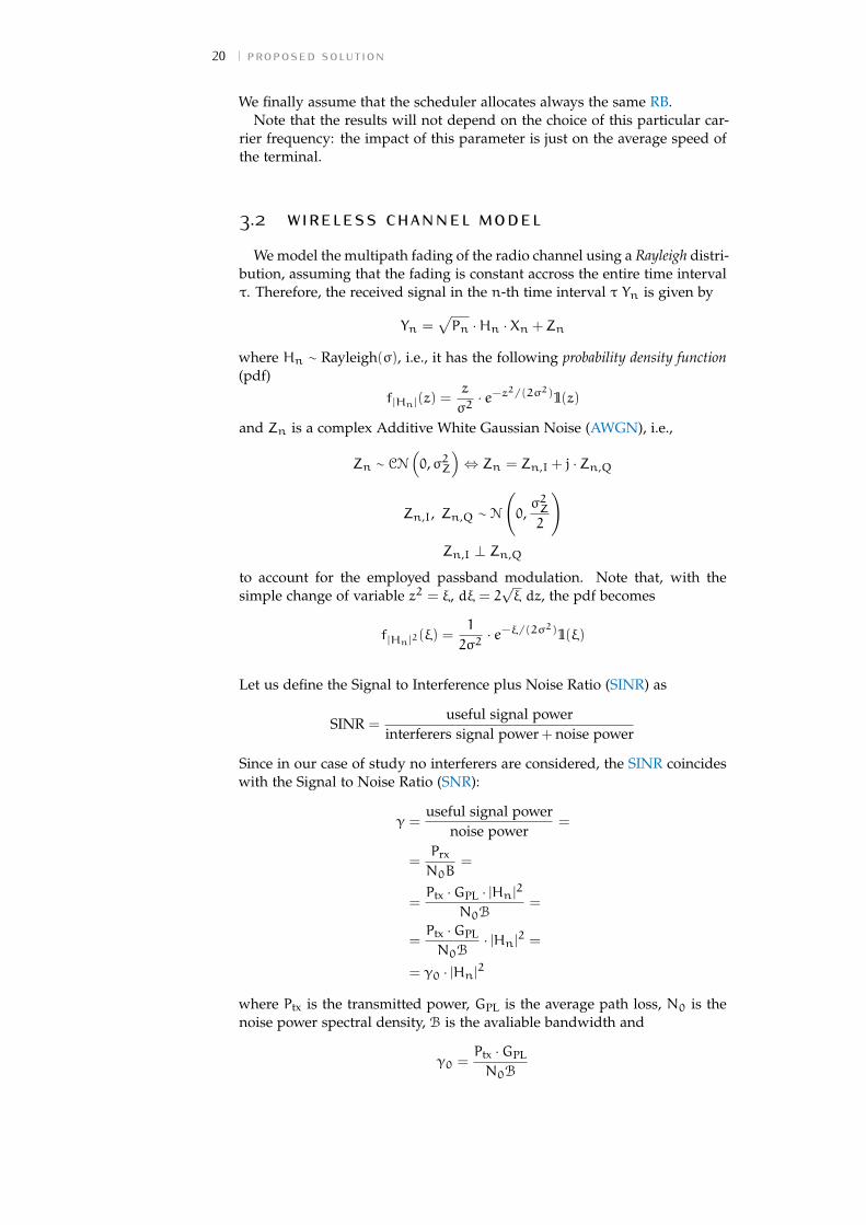
3.2 wireless channel modelWe model the multipath fading of the radio channel using a Rayleigh distri-
bution, assuming that the fading is constant accross the entire time intervalτ. Therefore, the received signal in the n-th time interval τ Yn is given by
Yn =√Pn ·Hn ·Xn +Zn
where Hn ∼ Rayleigh(σ), i.e., it has the following probability density function(pdf)
f|Hn|(z) =z
σ2· e−z
2/(2σ2)1(z)
and Zn is a complex Additive White Gaussian Noise (AWGN), i.e.,
Zn ∼ CN(0,σ2Z
)⇔ Zn = Zn,I + j ·Zn,Q
Zn,I, Zn,Q ∼ N
(0,σ2Z2
)Zn,I ⊥ Zn,Q
to account for the employed passband modulation. Note that, with thesimple change of variable z2 = ξ, dξ = 2
√ξ dz, the pdf becomes
f|Hn|2(ξ) =1
2σ2· e−ξ/(2σ
2)1(ξ)
Let us define the Signal to Interference plus Noise Ratio (SINR) as
SINR =useful signal power
interferers signal power + noise power
Since in our case of study no interferers are considered, the SINR coincideswith the Signal to Noise Ratio (SNR):
γ =useful signal power
noise power=
=Prx
N0B=
=Ptx ·GPL · |Hn|2
N0B=
=Ptx ·GPL
N0B· |Hn|2 =
= γ0 · |Hn|2
where Ptx is the transmitted power, GPL is the average path loss, N0 is thenoise power spectral density, B is the avaliable bandwidth and
γ0 =Ptx ·GPL
N0B

3.3 cqi model 21
is the average SNR. Since we don’t consider power control and the distancebetween the transmitter and the receiver is fixed, γ0 constant; therefore theuncertainty on the value of γ resides only in the multipath fading value
|Hn|2 =
γ
γ0
If we include the average fading power into the path loss term γ0 then wehave
E[|Hn|2] = 2σ2 = 1
and applying the change of variabile ξ = γγ0
, dξ = 1γ0dγ then we obtain
fΓ (γ) =1
γ0· e−γ/γ01(γ)
which is the SNR pdf in presence of Rayleigh multipath fading. The graphicrepresentation of the pdf is shown in Figure 9.
0 5 10 15 20 25 300
5 · 10−2
0.1
0.15
0.2
0.25
0.3
γ
f Γ(γ)
Figure 9: Probability density function of the signal-to-noise ratio in case of Rayleighfading. In this picture the average SNR is equal to 5 dB.
3.3 cqi modelAs explained in Chapter 1, a very important parameter in the LTE cel-
lular system is the Channel Quality Indicator (CQI), which represents ameasurement of the channel state that is reported to the source (the UE)by the destination (the eNB), together with the acknowledgement or not-acknowledgement of the previouly transmitted packet and many other in-formations about the network and the system status. The source tunes theparameters of the next packet transmission according to the last CQI valuein the case of uplink transmission.
According to Østerbø, 2011, numerical simulations show that the relation-ship between the CQI value and the actual SNR of the channel expressed indB is a simple linear transformation:
Γk,dB = 10 · log10 Γk∆= k · a+ b
22 proposed solution
or equivalently
Γk∆= 10
ka+b10
In LTE there exist N = 15 integer CQI values; the author of the cited articlestates that it is good practise to impose that
Γ1,dB = a+ b∆= −6 dB
Γ15,dB = 15a+ b∆= 20 dB
gettinga = 13/7
b = −55/7
Knowing a and b, it is possible to compute all the threshold values for theSNR Γ .
Note that this approach is in practise a quantization of the channel quality,where
Γ1,dB = a+ b and Γmax,dB∆= 20a+ b
are the boundaries of the granular region, in which the quantization error isfinite. Since we want to model the system for different average SNR valuesγ0, we modify the proposed boundaries, imposing that
Γ1,dB = a+ b = −30 dBΓ15,dB = 15a+ b = 20 dB
and gettinga = 25/7
b = −235/7
For what concerns the reconstruction levels Γk of such a quantization proce-dure, we recall from the theory of source coding that the optimal represen-tative values of each interval are by definition the centroids of the decisionregions, i.e.,
Γk∆=
∫Γk+1Γk
γ · fΓ |Γ∈[Γk,Γk+1](γ|γ ∈ [Γk, Γk+1]) dγ =
=
∫Γk+1Γk
γ · fΓ (γ) dγ∫Γk+1Γk
fΓ (γ) dγ
In our theoretical model we will consider for sake of simplicity that the SNRcan take values only in the finite set of the reconstruction levels, i.e.,
γ ∈ {Γk}k=1,...,15
Knowking the statistics of the SNR, we then compute the CQI stationaryprobabilities as
πk∆= P[CQI = k] = P[γ ∈ [Γk, Γk+1)] =
∫Γk+1Γk
fΓ (γ) dγ ∀k = 1, . . . , 14
and for CQI index k = 15 we consider
P[CQI = 15] =∫Γmax
Γ15
fΓ (γ) dγ

3.4 channel transitions model 23
Table 2: SNR thresholds for the computation of the CQI by the receiver for an aver-age SNR γ0,dB of 5 dB.
CQI k Γk,dB Γk πk Γk
1 −30.0000 0.0010 0.0004 0.00162 −26.4286 0.0023 0.0009 0.00373 −22.8571 0.0052 0.0021 0.00854 −19.2857 0.0118 0.0047 0.01935 −15.7143 0.0268 0.0107 0.04396 −12.1429 0.0611 0.0239 0.09987 −8.5714 0.1389 0.0522 0.22688 −5.0000 0.3162 0.1084 0.51379 −1.4286 0.7197 0.2008 1.156610 2.1429 1.6379 0.2882 2.568511 5.7143 3.7276 0.2394 5.530812 9.2857 8.4834 0.0662 11.280713 12.8571 19.3070 0.0022 22.459114 16.4286 43.9397 0.0000 47.102015 20.0000 100.0000 0.0000 103.1623
in such a way that
15∑k=1
P[CQI = k] =∫Γmax
Γ1
fΓ (γ) dγ = 1
since the design of the boundaries of the granular region Γ1 and Γmax is goodenough.
An example of a set of values for the probabilities πk for an average SNRγ0,dB of 5 dB can be found in the Table 2 too and is graphically representedin Figure 11.
3.4 channel transitions modelThe wireless channel we are considering may be either slow fading, i.e.,
the CQI index does not change much between subsequent time intervalsτ, or fast fading, i.e., the CQI index may experience large variations amongsubsequent transmission attempts. We assess the speed of the time variationsof the channel through the maximum Doppler frequency (also called Dopplershift) fm of the channel:
• if fm < 15 Hz then the channel can be considered slow fading
• if fm > 30 Hz then the channel can be considered fast fading
• for 15 6 fm 6 30 Hz the channel has an intermediate behaviour.
Since by definition
fm∆=v
λ
the considered Doppler shift accounts for a transmitter moving at an averagespeed
v = fm · λ
so the higher the Doppler shift is the faster the transmitter moves.

24 proposed solution
0 5 10 15 20 25 300
5 · 10−2
0.1
0.15
0.2
0.25
0.3
γ
f Γ(γ)
Figure 10: Example of Rayleigh fading channel quantization procedure. In this casethe average SNR is 5 dB; the vertical blue lines indicate the boundaries ofthe decision regions (the CQI boundaries), whereas the vertical red onesindicate the reconstruction levels.
1 2 3 4 5 6 7 8 9 10 11 12 13 14 150
5 · 10−2
0.1
0.15
0.2
0.25
0.3
0.35
0.4
0.45
0.5
CQI index i
πi
Figure 11: Example of stationary probabilities πi of the wireless channel. The aver-age SNR is γ0,dB = 5 dB.

3.5 rate matching process model 25
To characterize values of a Rayleigh fading channel at different time in-stants, we introduce the bivariate Rayleigh pdf :
fR1,R2(r1, r2, r) = 4r1r21− r
· e−r21+r22
1−r · I0(2r1r21− r
√r
)where
• R1 and R2 are the random varibles associated to the two instants
• r1, r2 are the associated values of the fading envelope
• I0(x) is the modified Bessel function of first type and order 0:
I0(x)∆=1
π
∫π0ex cosθ dθ
• r = ρ2, where ρ is the Bessel function of first type and order 0:
ρ∆= J0(2πfmτ)
Note that τ is the time displacement between the random variables,i.e., τ = 8 · TTI = 8 ms.
Recalling that|Hn|
2 =γ
γ0
we can compute the transition probabilities of the channel as
pi,j = P[j|i] =P[i, j]P[i]
=1
πi·∫√Γi+1/γ0√Γi/γ0
∫√Γj+1/γ0√Γj/γ0
fR1,R2(r1, r2, r) dr1dr2
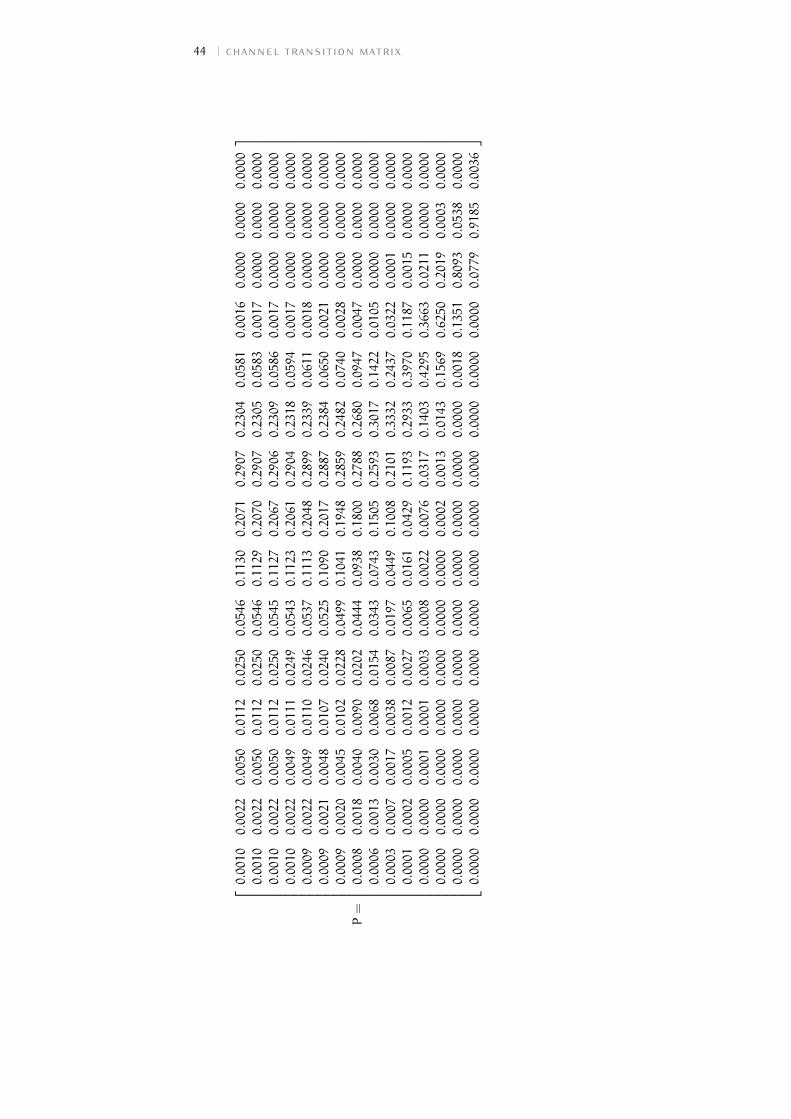
An example of channel transition matrix we obtain for γ0,dB = 5 dB isreported in the Appendix A on page 43.
3.5 rate matching process modelLTE employs a particular kind of rate matching process, which is difficult
to characterize from an analytical point of view, since it is a mix of IR-HARQand CC-HARQ. According to Cheng, 2008, the LTE rate matching processhas to extract from the circular buffer 4 different subsets, denoted by RV, ofthe codeword for different transmission attempts of a single packet. Giventhat the interleaver is well-designed, it is known that most of the Hammingweight for turbo codes resides in the parity bits: if eccessive puncturingis applied to them then the effective minimum distance of the puncturedcode degrades at high code rates. Therefore, a small amount of systematicbit puncturing has been proposed in literature. In the case of LTE ratematching process the fraction of punctured systematic bits is 1/16 ' 6%.The structure of the circular buffer can be graphically represented as inFigure 12. We denote
• X as the number of systematic bits
• T as the number of transmitted bits
• Y as the number of punctured bits

26 proposed solution
We recall the relation among these variables:
T∆= 3X− Y = (3− η)X
where η ∆= Y/X is the ratio between the punctured bits and the systematicbits. Observing Figure 12 we can note that:
• the size of the circular buffer is 3X, since the mother code rate of theturbo code is 1/3;
• the systematic bit stream starts at 0, whereas the interlaced paritystreams instead at X, with a phase displacement of π/3;
• the different RVs start at 3X4 i+116X, where i is the index of the RV,
and . . .
• they end at 3X4 i+ T +116X = 3X
4 i+ (3− η)X+ 116X
Note that the RV start points divide the circular buffer into 4 sectors ofthe same size 3X/4. Knowing the value of
T = (3− η)X = f(η)
we are able to determine in which one of the 4 sectors of the buffer thepattern ends up to be and how many loops we need to go through. Inthis way there can be found 7 distinct rate matching processes to describeall the possibilities in terms of CQI: the complete assignments of the CQIvalues to the models can be found in Table 3 and all the relationships forthe different transmission attempts are reported in Appendix B on page 45.Note that if η < 0 it means that there are some repeated bits already in thefirst transmission attempt, i.e., T = (3− η)X > 3X and the effective code rateconsidering the repeated bits is R(0)c,REP < 1/3.
Note, also, that if we consider both the RV start and end points then wecan divide the circular buffer into 8 sectors of just 2 different sizes (due to thesimmetry of the structure) that depend on the value of T . Note that, in thosecases in which 3Xi/4+ T > 3X for some retransmission index i ∈ {0, 1, 2, 3},some sectors are transmitted more than once, experiencing different SNRs.
3.6 enhanced rate characterizationIn Chapter 2 we already explained a method to characterize analytically
the code rates for subsequent transmission attempts in LTE. We now pro-pose an enhancement of that model to provide an exact code rate computa-tion. The effective code rate after the i-th transmission attempt consideringrepeated bits can be computed as follows:
R(i)c,REP =
number of information bits that are sent till tx attempt inumber of total bits that are sent till tx attempt i
=
=
1516X
3X4 i+ T
if3X
4i+ T < 3X−
X
16
1516X+
[3X4 i+ T −
(3X− X
16
)]3X4 i+ T
if 3X−X
1663X
4i+ T < 3X
X3X4 i+ T
otherwise

3.7 how to model the accumulated mutual information in lte? 27
Figure 12: Representation of the virtual circular buffer employed during the bit se-lection procedure. Note the presence of a non-zero displaced startingposition for the RV of index 0: this is done on purpose to maximize theturbo decoding procedure performances, which become poor in case ofexcessive parity bits punturing, especially for high code rates.
where i ∈ {0, 1, 2, 3}. We recall that
R(i)c = max
{R(i)c,REP ;
1
3
}The new code rates obtained following this approach are reported in Table 3
and graphically represented in Figure 13.The new values of η for all the CQI indexes can still be computed knowing
the values of R(0)c,REP, similarly to what has been done in Chapter 2; they canbe found in Table 3.
3.7 how to model the accumulated mutualinformation in lte?
Given the rate matcher characterization of the previous section, we cancharacterize the ACMI modeling a mixed Incremental Redundancy (IR) andChase Combining (CC) HARQ:
I?(γ) =
k∑i=1
λi ·C
m∑j=1
αijγj
where
• C(x) = log2(1+ x) is the capacity of complex valued AWGN channel
• k is the number of sectors in which the circular buffer is partitioned,so it is k = 8

28 proposed solution
1 2 3 4 5 6 7 8 9 10 11 12 13 14 150.30.350.40.450.50.550.60.650.70.750.80.850.90.951
CQI index i
Rc
Tx attempt #1
Tx attempt #2
Tx attempt #3
Tx attempt #4
Figure 13: MCS for subsequent transmission attempts obtained using the enhancedapproach. The coding rates are effective and compute without consider-ing the repeated bits.
Table 3: The value of the puncturing patterns obtained using the enhanced solutionare listed in column 3. In column 4 there can be found the mapping be-tween CQI values and rate matcher models: depending on the position ofη in the circular buffer, a different rate matcher model must be applied tocharacterize the ACMI.
CQI k Modulation η R(0)c,REP Rate matcher model
1 QPSK −10.1300 0.076 #72 QPSK −5.5300 0.12 #63 QPSK −2.3100 0.19 #54 QPSK −0.3200 0.30 #45 QPSK 0.8625 0.44 #26 QPSK 1.4062 0.59 #2
7 16-QAM 0.4594 0.37 #38 16-QAM 1.0406 0.48 #29 16-QAM 1.4438 0.60 #2
10 64-QAM 0.9375 0.45 #211 64-QAM 1.3031 0.55 #212 64-QAM 1.5562 0.65 #113 64-QAM 1.7531 0.75 #114 64-QAM 1.9031 0.85 #115 64-QAM 1.9875 0.93 #1

3.8 markov chain 29
• m ∈ {1, 2, 3, 4} is the transmission attempt index
• γ = [γ1 . . . γm]T is the vector that collects the SNR values that areexperienced during the m subsequent transmission attempts
• αij is the number of times that sector i in the circular buffer experi-ences the SNR γj; it is
0 6 αij 6 m
• λi is the fraction of bits that belongs to sector iwith respect to the totalsent bits, without considering repeated bits. We always have that
k∑i=1
λi = 1
3.8 markov chainTo analyze the process of HARQ and rate matching we propose a Markov
chain, which provides a good representation of the system. However wewill evaluate the behaviour of the chain using numerical evaluations due tothe complexity of such a model.
3.8.1 Structure of the chainThe states of the Markov chain we propose are triplets:
(Kn,Xn,CQIn)
where
• Kn ∈ {0, 1, 2, 3, 4} is the number of attempts done by the transmitter todeliver the current packet; if Kn = 0 it means that a new packet hasjust started its transmission round
• Xn is the value of the ACMI at the n-th transmission attempt; if Kn = 0
then it follows that X0∆= 0
• CQIn is the CQI index experienced during the n-th transmission at-tempt; if Kn = 0 then CQIn is just the CQI value of the previouspacket last transmission attempt and it is used to select the appropri-ate MCS for the next packet transmission.
The total number of states is upper bounded by 155 = 759375, but, since inmany cases it is not possible to reach all other states from any state of thechannel, the cardinality of the set of states is in practise
|S|� 155
3.8.2 RewardsWe distinguish between two kinds of rewards:
1. R is the number of information bits which have been delivered at theend of a transmission round of a certain packet. We have that
R =
{R(i)c · log2M if the i-th retx attempt is successful0 if the 3rd retx attempt fails

30 proposed solution
2. T is the delay introduced by the retransmission process. Since we aretaking into account a synchronous HARQ process, the value of T is
discrete: it is a multiple of τ ∆= 8 · TTI. We have that
T =
{(i+ 1) · τ if the i-th retx attempt is successful4 · τ if the 3rd retx attempt fails
The complete characterization of the proposed Markov model is availablein Appendix C on page 55.
3.9 the bayesian approachOur aim now is that of introducing some kind of knowledge from past
states of the channel and try to predict the channel behaviour in order toimprove system performances. Let’s give an example: the transmitter hasjust experienced a generic quadruple of CQI values (a path of CQIs)
CQIa → CQIb → CQIc → CQId
where CQIa is the CQI relative to the first transmission attempt and so it isthe one that defines the modulation and coding schemes that has to be used.In this case the path length L is equal to 4, but in general we have that
1 6 L 6 4
where the two boundaries L = 1 and L = 4 correspond to the best case,in which the transmission is immediately successful, and the worst case, inwhich we employ all possible transmission attempts, respectively. Excludingthe best case, in all other cases we encounter inefficiencies in terms of accu-mulated delay due to the retransmission process. In every case, the MCS forthe transmission of the following packet is selected according to the valueof CQId, discarding the information relative to the rest of the path.
Now, we want to gain advantage of the knowledge of the history of theprevious transmission. To do so, in those cases in which the previous trans-mission required at least one retransmission, i.e., L > 2, we let the transmit-ter compute the average value of the CQI experienced during the last packetdelivery as
CQI ∆=1
L
L∑k=1
CQIk
This is the learning phase of the Bayesian approach. Then the planning takesplace:
• if dCQIe > CQId then we could think of trying to be more aggressive,employing the MCS defined by dCQIe
• otherwise we proceed as usual and employ the MCS defined by CQId.
Finally the transmitter acts, using the appropriate MCS for the next trans-mission round.

4 P E R F O R M A N C E E VA L U AT I O NIn this Chapter we show the results of the proposed model obtained via
numerical evaluation. The behaviour of the Markov chain in the long termhas been numerically evaluated using Matlab, simulating the channel tran-sitions and the accumulation of the mutual information among subsequenttransmissions.
4.1 simulation procedureDue to the complexity of the proposed Markov chain, its performances
have been evaluated using a discrete-time simulation. Table 4 contains theparameters that have been used for the simulation.
We have considered an average SNR range of [−10, 30] dB. The simulationconsists of the following steps:
1. Start from the channel state relative to the CQI with the highest sta-tionary probability π?i = maxj{πj}.
2. Select the digital modulation order and the code rates for the entiretransmission round of the packet (initial transmission and the 3 possi-ble retransmissions) according to the current start state.
3. Select the appropriate rate matching model with respect to the currentstart state.
4. Perform the subsequent transmission attempts, evaluating the appro-priate formula for the ACMI for each attempt.
5. Tune the next packet transmission round according to the last expe-rienced CQI index (default procedure) or following the Bayesian ap-proach (enhanced procedure).
6. Repeat from step 2. for a certain fixed number of packets.
7. Compute averages and confidence intervals.
Table 4: In this Table are reported the simulation parameters that have been used toevaluate the long term behaviour of the proposed Markov chain. These pa-rameters guarantees that the confidence intervals are approximately equalto zero.
Parameter Value
minimum γ0,dB −10 dBmaximum γ0,dB 30 dB
Montecarlo simulations 50
number of generated packets 5000
TTI 0.001 s
31

32 performance evaluation
4.1.1 Possible enhancementsA possible enhancement of the model could be that of generating a ran-
dom SNR sample in every CQI interval: this can be done using the rejectionmethod.
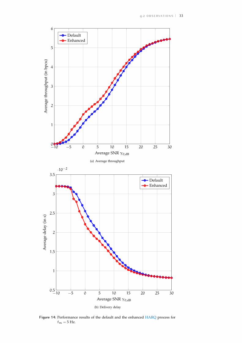
4.2 observationsThe results of the numerical evaluation of the system bahviour are shown
in Figures 14, 15, 17, 18 and 19.
4.2.1 TrendsTwo quantities have been considered:
throughput The throughput is approximately equal to zero for low aver-age SNR values and increases as the average SNR increase; we notethat the throughput tends to saturate for high average SNR values.
delay The delivery delay is maximum for lower average SNR values andit decreases as the average SNR increase. It tends to saturate for highSNRs too.
4.2.2 Comparison with real simulatorsThe trend of the curves is expected and similar to the real simulators, like
the Vienna simulator (see Blumenstein et al., 2011).
4.2.3 Enhancement of the model: does it work?It can be seen that the enhanced model guarantees a higher throughput
while decreasing the delivery delay with respect to the default model. In-deed there is a gap between the standard approach and the intelligent one:the latter provides the same performances of the former for lower averageSNR values. However the size of that gap depends on how much correlatedthe channel is. Indeed
• if the channel is slow fading (low Doppler frequency, fm ∈ [5, 20] Hz)then the gap is quite large
• if the channel is fast fading (high Doppler frequency, fm > 30 Hz) thenthe gap is closed.
One can conclude, therefore, that applying this kind of intelligence is worthwhen the channel is correlated.
4.2 observations 33
−10 −5 0 5 10 15 20 25 300
1
2
3
4
5
6
Average SNR γ0,dB
Ave
rage
thro
ughp
ut(i
nbp
cu)
DefaultEnhanced
(a) Average throughput
−10 −5 0 5 10 15 20 25 300.5
1
1.5
2
2.5
3
3.5·10−2
Average SNR γ0,dB
Ave
rage
dela
y(i
ns)
DefaultEnhanced
(b) Delivery delay
Figure 14: Performance results of the default and the enhanced HARQ process forfm = 5 Hz.

34 performance evaluation
−10 −5 0 5 10 15 20 25 300
1
2
3
4
5
6
Average SNR γ0,dB
Ave
rage
thro
ughp
ut(i
nbp
cu)
DefaultEnhanced
(a) Average throughput
−10 −5 0 5 10 15 20 25 300.5
1
1.5
2
2.5
3
3.5·10−2
Average SNR γ0,dB
Ave
rage
dela
y(i
ns)
DefaultEnhanced
(b) Delivery delay
Figure 15: Performance results of the default and the enhanced HARQ process forfm = 10 Hz.

4.2 observations 35
−10 −5 0 5 10 15 20 25 300
1
2
3
4
5
6
Average SNR γ0,dB
Ave
rage
thro
ughp
ut(i
nbp
cu)
DefaultEnhanced
(a) Average throughput
−10 −5 0 5 10 15 20 25 300.5
1
1.5
2
2.5
3
3.5·10−2
Average SNR γ0,dB
Ave
rage
dela
y(i
ns)
DefaultEnhanced
(b) Delivery delay
Figure 16: Performance results of the default and the enhanced HARQ process forfm = 15 Hz.

36 performance evaluation
−10 −5 0 5 10 15 20 25 300
1
2
3
4
5
6
Average SNR γ0,dB
Ave
rage
thro
ughp
ut(i
nbp
cu)
DefaultEnhanced
(a) Average throughput
−10 −5 0 5 10 15 20 25 300.5
1
1.5
2
2.5
3
3.5·10−2
Average SNR γ0,dB
Ave
rage
dela
y(i
ns)
DefaultEnhanced
(b) Delivery delay
Figure 17: Performance results of the default and the enhanced HARQ process forfm = 20 Hz.

4.2 observations 37
−10 −5 0 5 10 15 20 25 300
1
2
3
4
5
6
Average SNR γ0,dB
Ave
rage
thro
ughp
ut(i
nbp
cu)
DefaultEnhanced
(a) Average throughput
−10 −5 0 5 10 15 20 25 300.5
1
1.5
2
2.5
3
3.5·10−2
Average SNR γ0,dB
Ave
rage
dela
y(i
ns)
DefaultEnhanced
(b) Delivery delay
Figure 18: Performance results of the default and the enhanced HARQ process forfm = 30 Hz.

38 performance evaluation
−10 −5 0 5 10 15 20 25 300
1
2
3
4
5
6
Average SNR γ0,dB
Ave
rage
thro
ughp
ut(i
nbp
cu)
DefaultEnhanced
(a) Average throughput
−10 −5 0 5 10 15 20 25 300.5
1
1.5
2
2.5
3
3.5·10−2
Average SNR γ0,dB
Ave
rage
dela
y(i
ns)
DefaultEnhanced
(b) Delivery delay
Figure 19: Performance results of the default and the enhanced HARQ process forfm = 40 Hz.

5 C O N C L U S I O N A N D F U T U R EW O R K
In this thesis we propose a theoretical model based on Markov chainsto study the Hybrid Automatic Repeat reQuest (HARQ) process of LongTerm Evolution (LTE) cellular network technology. In particular, we havebeen focusing on a single HARQ process in the uplink channel: after areview of the state of the art, we first decided to account for a Rayleighfading channel with Additive White Gaussian Noise (AWGN) noise; thenwe studied the rate matching process from an analytical point of view, in-troducing an expression of the ACcumulated Mutual Information (ACMI)taylored to the LTE rate matcher and designed a Markov model to evalu-ate the long term behaviour of the system. We also proposed a bayesianapproach in which the system exploits the gathered information about thepast channel states, trying to employ more aggressive Modulation and Cod-ing Schemes (MCSs) when it is possible. Due to the complexity of sucha model, the performances have been evaluated through numerical simula-tions: the results show that the proposed enhancement to the system pro-vides an higher throughput and a lower delivery delay with respect to thedefault protocol for channels with low mobility.
Future works will include a further study of the enhanced system andthe extension of the model to other kind of channels and to Multi-InputMulti-Output (MIMO).
39


C O N C L U S I O N I E S V I L U P P IF U T U R I
In questo elaborato viene proposto un modello di tipo Markoviano perstudiare i processi di Hybrid Automatic Repeat reQuest (HARQ) impiegatinel sistema cellulare Long Term Evolution (LTE). In particolare ci siamo fo-calizzati su un singolo processo di HARQ nell’uplink: dopo aver esaminatolo stato dell’arte, si è deciso di considerare un canale con un’attenuazione diRayleigh e rumore additivo gaussiano bianco (AWGN); quindi è stato ana-lizzato il processo di rate matching, introducendo un’apposita espressioneper l’informazione mutua accumulata (ACMI) per descriverne il comporta-mento; infine è stato proposto un modello di tipo Markoviano per valutarele prestazioni del sistema a lungo termine. É stato presentato, inoltre, unapproccio di tipo bayesiano in cui il sistema sfrutta le informazioni raccoltesui precedenti stati del canale wireless, tentando di utilizzare modulazionie rate di codifica più aggressivi quando possibile. A causa della complessitàdi tale modello, le prestazioni sono state valutate numericamente: i risultatidimostrano che il miglioramento proposto garantisce un maggiore through-put a fronte di un minor ritardo rispetto al protocollo predefinito per canalia bassa mobilità.
Gli sviluppi futuri comprendono uno studio approfondito del migliora-mento apportato al sistema e l’estensione del modello ad altre tipologie dicanale e al MIMO.
41


A C H A N N E L T R A N S I T I O NM AT R I X
In this Appendice we show an example of a transition matrix for theRayleigh fading channel we have considered for our theoretical model. Ithas been computed numerically evaluating the bivariate Rayleigh pdf
fR1,R2(r1, r2, r) = 4r1r21− r
· e−r21+r22
1−r · I0(2r1r21− r
√r
)where
• R1 and R2 are the random varibles associated to the two points
• r1, r2 are the associated values of the envelope
• I0(x) is the modified Bessel function of first type and order 0:
I0(x)∆=1
π
∫π0ex cosθ dθ
• r = ρ2, where ρ is the Bessel function of first type and order 0:
ρ∆= J0(2πfmτ)
• fm = Doppler shift
• τ = 8 · TTI = 8 ms
in the appropriate rectangular area[√
Γiγ0
,√Γi+1γ0
]×[√
Γjγ0
,√Γj+1γ0
], so that
pi,j = P[j|i] =P[i, j]P[i]
=1
πi·∫√Γi+1/γ0√Γi/γ0
∫√Γj+1/γ0√Γj/γ0
fR1,R2(r1, r2, r) dr1dr2
In this example we consider an average SNR γ0,dB = 5 dB and a Dopplershift fm = 20 Hz. Since we consider fc = 1930 Hz, we have that the averagespeed of the transmitter is
v =fm
λ= 3.1067 m/s = 11.184 km/h
The complete matrix can be found in the following page.
43
44 channel transition matrix
P=
0.00100
.00220
.00500
.01120
.02500
.05460
.11300
.20710
.29070
.23040
.05810
.00160
.00000
.00000
.0000
0.00100
.00220
.00500
.01120
.02500
.05460
.11290
.20700
.29070
.23050
.05830
.00170
.00000
.00000
.0000
0.00100
.00220
.00500
.01120
.02500
.05450
.11270
.20670
.29060
.23090
.05860
.00170
.00000
.00000
.0000
0.00100
.00220
.00490
.01110
.02490
.05430
.11230
.20610
.29040
.23180
.05940
.00170
.00000
.00000
.0000
0.00090
.00220
.00490
.01100
.02460
.05370
.11130
.20480
.28990
.23390
.06110
.00180
.00000
.00000
.0000
0.00090
.00210
.00480
.01070
.02400
.05250
.10900
.20170
.28870
.23840
.06500
.00210
.00000
.00000
.0000
0.00090
.00200
.00450
.01020
.02280
.04990
.10410
.19480
.28590
.24820
.07400
.00280
.00000
.00000
.0000
0.00080
.00180
.00400
.00900
.02020
.04440
.09380
.18000
.27880
.26800
.09470
.00470
.00000
.00000
.0000
0.00060
.00130
.00300
.00680
.01540
.03430
.07430
.15050
.25930
.30170
.14220
.01050
.00000
.00000
.0000
0.00030
.00070
.00170
.00380
.00870
.01970
.04490
.10080
.21010
.33320
.24370
.03220
.00010
.00000
.0000
0.00010
.00020
.00050
.00120
.00270
.00650
.01610
.04290
.11930
.29330
.39700
.11870
.00150
.00000
.0000
0.00000
.00000
.00010
.00010
.00030
.00080
.00220
.00760
.03170
.14030
.42950
.36630
.02110
.00000
.0000
0.00000
.00000
.00000
.00000
.00000
.00000
.00000
.00020
.00130
.01430
.15690
.62500
.20190
.00030
.0000
0.00000
.00000
.00000
.00000
.00000
.00000
.00000
.00000
.00000
.00000
.00180
.13510
.80930
.05380
.0000
0.00000
.00000
.00000
.00000
.00000
.00000
.00000
.00000
.00000
.00000
.00000
.00000
.07790
.91850
.0036

B R AT E M ATC H I N G M O D E L I N GA N D A C M I
We recall briefly some notation:
• X = number of systematic bits
• 3X = size of the circular buffer
• T = 3X− Y = (3− YX )X = (3− η)X = number of sent bits
• Y = number of punctured bits
• R(m−1)c = effective code rate after the m-th transmission, without con-
sidering repeated bits
• R(m) = information rate of the m-th transmission attempt
and the formula for the ACMI computation:
I?(γ) =
k∑i=1
λi ·C
m∑j=1
αijγj
where
• C(x) = log2(1+ x) is the capacity of complex valued AWGN channel
• k is the number of sectors in which the circular buffer is partitioned,so it is k = 8
• m ∈ {1, 2, 3, 4} is the transmission attempt index
• γ = [γ1 . . . γm]T is the vector that collects the SNR values that areexperienced during the m subsequent transmission attempts
• αij is the number of times that sector i in the circular buffer experi-ences the SNR γj; it is
0 6 αij 6 m
• λi is the fraction of bits that belongs to sector iwith respect to the totalsent bits, without considering repeated bits. We always have that
k∑i=1
λi = 1
b.1 rate matching #10 6 T <
3
2X
• 1st transmission attempt
C(γ1) ≷ R(1) = R
(0)c · log2M
45

46 rate matching modeling and acmi
Figure 20: Graphical representation of the first type of rate matcher. The first trans-mission attempt is in red, the second in blue, the third in green and thefourth in black.
• 2nd transmission attempt
3/4
15/4− η·C(γ1)+
9/4− η
15/4− η·C(γ1+γ2)+
3/4
15/4− η·C(γ2) ≷ R(2) = R
(1)c · log2M
• 3rd transmission attempt
3/4
9/2− η·C(γ1) +
9/4− η
9/2− η·C(γ1 + γ2) +
η− 3/2
9/2− η·C(γ2)+
+9/4− η
9/2− η·C(γ2 + γ3) +
3/4
9/2− η·C(γ3) ≷ R(3) = R
(2)c · log2M
• 4th transmission attempt
9/4− η
3·C(γ1 + γ4) +
η− 3/2
3·C(γ1) +
9/4− η
3·C(γ1 + γ2)+
+η− 3/2
3·C(γ2) +
9/4− η
3·C(γ2 + γ3) +
η− 3/2
3·C(γ3)+
+9/4− η
3·C(γ3 + γ4) +
η− 3/2
3·C(γ4) ≷ R(4) = R
(3)c · log2M
b.2 rate matching #23
2X 6 T <
9
4X
• 1st transmission attempt
C(γ1) ≷ R(1)

b.3 rate matching #3 47
Figure 21: Graphical representation of the second type of rate matcher. The firsttransmission attempt is in red, the second in blue, the third in green andthe fourth in black.
• 2nd transmission attempt
3/4
15/4− η·C(γ1) +
9/4− η
15/4− η·C(γ1 + γ2) +
3/4
15/4− η·C(γ2) ≷ R(2)
• 3rd transmission attempt
3/2− η
3·C(γ1 + γ3) +
η− 3/4
3·C(γ1) +
3/4
3·C(γ1 + γ2)+
+3/2− η
3·C(γ1 + γ2 + γ3) +
3/4
3·C(γ2 + γ3) +
η− 3/4
3·C(γ3) ≷ R(3)
• 4th transmission attempt
3/2− η
3·C(γ1 + γ3 + γ4) +
η− 3/4
3·C(γ1 + γ4) +
3/2− η
3·C(γ1 + γ2 + γ4)+
+η− 3/4
3·C(γ1 + γ2) +
3/2− η
3·C(γ1 + γ2 + γ3) +
η− 3/4
3·C(γ2 + γ3)+
+3/2− η
3·C(γ2 + γ3 + γ4) +
η− 3/4
3·C(γ3 + γ4) ≷ R(4)
b.3 rate matching #39
4X 6 T < 3X
• 1st transmission attempt
C(γ1) ≷ R(1)

48 rate matching modeling and acmi
Figure 22: Graphical representation of the third type of rate matcher. The first trans-mission attempt is in red, the second in blue, the third in green and thefourth in black.
• 2nd transmission attempt
3/4− η
3·C(γ1 + γ2) +
η
3·C(γ1) +
9/4− η
3·C(γ1 + γ2) +
η
3·C(γ2) ≷ R(2)
• 3rd transmission attempt
3/4− η
3·C(γ1 + γ2 + γ3) +
η
3·C(γ1 + γ3) +
3/4− η
3·C(γ1 + γ2 + γ3)+
+η
3·C(γ1 + γ2) +
3/2− η
3·C(γ1 + γ2 + γ3) +
η
3·C(γ2 + γ3) ≷ R(3)
• 4th transmission attempt
3/4− η
3·C(γ1 + γ2 + γ3 + γ4) +
η
3·C(γ1 + γ3 + γ4)+
+3/4− η
3·C(γ1 + γ2 + γ3 + γ4) +
η
3·C(γ1 + γ2 + γ4)+
+3/4− η
3·C(γ1 + γ2 + γ3 + γ4) +
η
3·C(γ1 + γ2 + γ3)+
+3/4− η
3·C(γ1 + γ2 + γ3 + γ4) +
η
3·C(γ2 + γ3 + γ4) ≷ R(4)
b.4 rate matching #43X 6 T < 3X+
3
4X =
15
4X
• 1st transmission attempt
−η
3·C(2γ1) +
3+ η
3·C(γ1) ≷ R(1)

b.5 rate matching #5 49
Figure 23: Graphical representation of the fourth type of rate matcher. The firsttransmission attempt is in red, the second in blue, the third in green andthe fourth in black.
• 2nd transmission attempt
−η
3·C(2γ1 + γ2) +
3/4+ η
3·C(γ1 + γ2)+
+−η
3·C(γ1 + 2γ2) +
9/4+ η
3·C(γ1 + γ2) ≷ R(2)
• 3rd transmission attempt
−η
3·C(2γ1 + γ2 + γ3) +
3/4+ η
3·C(γ1 + γ2 + γ3) +
−η
3·C(γ1 + 2γ2 + γ3)+
+3/4+ η
3·C(γ1 + γ2 + γ3) +
−η
3·C(γ1 + γ2 + 2γ3) +
3/2+ η
3·C(γ1 + γ2 + γ3) ≷ R(3)
• 4th transmission attempt
−η
3·C(2γ1 + γ2 + γ3 + γ4) +
3/4+ η
3·C(γ1 + γ2 + γ3 + γ4)+
+−η
3·C(γ1 + 2γ2 + γ3 + γ4) +
3/4+ η
3·C(γ1 + γ2 + γ3 + γ4)+
+−η
3·C(γ1 + γ2 + 2γ3 + γ4) +
3/4+ η
3·C(γ1 + γ2 + γ3 + γ4)+
+−η
3·C(γ1 + γ2 + γ3 + 2γ4) +
3/4+ η
3·C(γ1 + γ2 + γ3 + γ4) ≷ R(4)
b.5 rate matching #53X+
9
4X 6 T < 6X
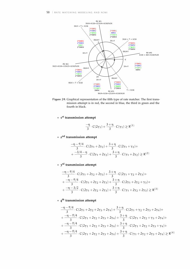
50 rate matching modeling and acmi
Figure 24: Graphical representation of the fifth type of rate matcher. The first trans-mission attempt is in red, the second in blue, the third in green and thefourth in black.
• 1st transmission attempt
−η
3·C(2γ1) +
3+ η
3·C(γ1) ≷ R(1)
• 2nd transmission attempt
−η− 9/4
3·C(2γ1 + 2γ2) +
3+ η
3·C(2γ1 + γ2)+
+−3/4− η
3·C(2γ1 + 2γ2) +
3+ η
3·C(γ1 + 2γ2) ≷ R(2)
• 3rd transmission attempt
−η− 9/4
3·C(2γ1 + 2γ2 + 2γ3) +
3+ η
3·C(2γ1 + γ2 + 2γ3)+
+−η− 9/4
3·C(2γ1 + 2γ2 + 2γ3) +
3+ η
3·C(2γ1 + 2γ2 + γ3)+
+−η− 3/2
3·C(2γ1 + 2γ2 + 2γ3) +
3+ η
3·C(γ1 + 2γ2 + 2γ3) ≷ R(3)
• 4th transmission attempt
−η− 9/4
3·C(2γ1 + 2γ2 + 2γ3 + 2γ4) +
3+ η
3·C(2γ1 + γ2 + 2γ3 + 2γ4)+
+−η− 9/4
3·C(2γ1 + 2γ2 + 2γ3 + 2γ4) +
3+ η
3·C(2γ1 + 2γ2 + γ3 + 2γ4)+
+−η− 9/4
3·C(2γ1 + 2γ2 + 2γ3 + 2γ4) +
3+ η
3·C(2γ1 + 2γ2 + 2γ3 + γ4)+
+−η− 9/4
3·C(2γ1 + 2γ2 + 2γ3 + 2γ4) +
3+ η
3·C(γ1 + 2γ2 + 2γ3 + 2γ4) ≷ R(4)

b.6 rate matching #6 51
b.6 rate matching #6
6X+9
4X 6 T < 9X
Figure 25: Graphical representation of the sixth type of rate matcher. The first trans-mission attempt is in red, the second in blue, the third in green and thefourth in black.
• 1st transmission attempt
−η− 3
3·C(3γ1) +
6+ η
3·C(2γ1) ≷ R(1)
• 2nd transmission attempt
−η− 21/4
3·C(3γ1 + 3γ2) +
6+ η
3·C(3γ1 + 2γ2)+
+−15/4− η
3·C(3γ1 + 3γ2) +
6+ η
3·C(2γ1 + 3γ2) ≷ R(2)
• 3rd transmission attempt
−η− 21/4
3·C(3γ1 + 3γ2 + 3γ3) +
6+ η
3·C(3γ1 + 2γ2 + 3γ3)+
+−η− 21/4
3·C(3γ1 + 3γ2 + 3γ3) +
6+ η
3·C(3γ1 + 3γ2 + 2γ3)+
+−η− 9/2
3·C(3γ1 + 3γ2 + 3γ3) +
6+ η
3·C(2γ1 + 3γ2 + 3γ3) ≷ R(3)

52 rate matching modeling and acmi
• 4th transmission attempt
−η− 21/4
3·C(3γ1 + 3γ2 + 3γ3 + 3γ4) +
6+ η
3·C(3γ1 + 2γ2 + 3γ3 + 3γ4)+
+−η− 21/4
3·C(3γ1 + 3γ2 + 3γ3 + 3γ4) +
6+ η
3·C(3γ1 + 3γ2 + 2γ3 + 3γ4)+
+−η− 21/4
3·C(3γ1 + 3γ2 + 3γ3 + 3γ4) +
6+ η
3·C(3γ1 + 3γ2 + 3γ3 + 2γ4)+
+−η− 21/4
3·C(3γ1 + 3γ2 + 3γ3 + 3γ4) +
6+ η
3·C(2γ1 + 3γ2 + 3γ3 + 3γ4) ≷ R(4)
b.7 rate matching #7
12X+3
4X 6 T < 12X+
3
2X
Figure 26: Graphical representation of the seventh type of rate matcher. The firsttransmission attempt is in red, the second in blue, the third in green andthe fourth in black.
• 1st transmission attempt
−η− 9
3·C(5γ1) +
12+ η
3·C(4γ1) ≷ R(1)
• 2nd transmission attempt
3/4
3·C(5γ1 + 4γ2) +
−η− 39/4
3·C(5γ1 + 5γ2)+
+3/4
3·C(4γ1 + 5γ2) +
45/4+ η
3·C(4γ1 + 4γ2) ≷ R(2)
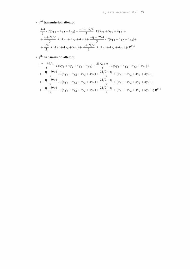
b.7 rate matching #7 53
• 3rd transmission attempt
3/4
3·C(5γ1 + 4γ2 + 4γ3) +
−η− 39/4
3·C(5γ1 + 5γ2 + 4γ3)+
+η+ 21/2
3·C(4γ1 + 5γ2 + 4γ3) +
−η− 39/4
3·C(4γ1 + 5γ2 + 5γ3)+
+3/4
3·C(4γ1 + 4γ2 + 5γ3) +
η+ 21/2
3·C(4γ1 + 4γ2 + 4γ3) ≷ R(3)
• 4th transmission attempt
−η− 39/4
3·C(5γ1 + 4γ2 + 4γ3 + 5γ4) +
21/2+ η
3·C(5γ1 + 4γ2 + 4γ3 + 4γ4)+
+−η− 39/4
3·C(5γ1 + 5γ2 + 4γ3 + 4γ4) +
21/2+ η
3·C(4γ1 + 5γ2 + 4γ3 + 4γ4)+
+−η− 39/4
3·C(4γ1 + 5γ2 + 5γ3 + 4γ4) +
21/2+ η
3·C(4γ1 + 4γ2 + 5γ3 + 4γ4)+
+−η− 39/4
3·C(4γ1 + 4γ2 + 5γ3 + 5γ4) +
21/2+ η
3·C(4γ1 + 4γ2 + 4γ3 + 5γ4) ≷ R(4)


C M A R KO V C H A I N G R A P H
In this Appendix you can find in Figure 27 the graph of the proposedMarkov model described in Chapter 3 on page 19.
0
X(0)
a
start
1
X(1)
b
2
X(2)
c
3
X(3)
d
4
X(4)
e
p0,1
p1,2
p1,0p2,1
p2,3
p3,0
p3,4
p4,0
Figure 27: Graphical representation of the proposed Markov model.
The graphical representation in Figure 27 is general and, at the same time,compact: illustrating the entire Markov chain would be unfeasible, indeed.We recall that every state consists of the triplet
(Kn,Xn, CQIn)
where
• Kn ∈ {0, 1, 2, 3, 4} is the number of attempts done by the transmitter todeliver the current packet; if Kn = 0 it means that a new packet hasjust started its transmission round
• Xn is the value of the ACMI at the n-th transmission attempt; if Kn = 0
then it follows that Xn = 0
• CQIn is the CQI index experienced during the n-th transmission at-tempt; if Kn = 0 then CQIn is just the CQI value of the previouspacket last transmission attempt, i.e., CQI n ≡ CQIn−1; this CQI valueis used to select the appropriate MCS for the next packet transmission.
In the graph we denote with X(i) the ACMI relative to the transmissionattempt Xn = i, i ∈ {0, 1, 2, 3, 4}. The random process starts from the state
55

56 markov chain graph
(0,X(0),a), where a = arg maxi
{πi}, and travels a random path, according to
the following transition probabilities:
p0,1 = P[CQIn = b | CQIn−1 = a]
p1,2 = P[X(1) 6 R(0)c · log2M , CQIn+1 = c | CQIn = b]
p2,3 = P[X(2) 6 R(1)c · log2M , CQIn+2 = d | CQIn+1 = c, CQIn = b]
p3,4 = P[X(3) 6 R(2)c · log2M , CQIn+3 = e | CQIn+2 = d, CQIn+1 = c, CQIn = b]
p1,0 = P[X(1) > R(0)c · log2M | CQIn = b]
p2,0 = P[X(2) > R(1)c · log2M | CQIn+1 = c, CQIn = b]
p3,0 = P[X(3) > R(2)c · log2M | CQIn+2 = d, CQIn+1 = c, CQIn = b]
p4,0 = 1
where the cardinality of the symbol alphabet M and the coding rate R(i−1)c
depend on the value of the CQI in the state (0, 0,a), i.e.,
M =M(a) and Rc = Rc(a)
The random rewards that we consider are
R1,0 = R(0)c · log2M
R2,0 = R(1)c · log2M
R3,0 = R(2)c · log2M
R4,0 =
{0 if X(4) 6 R(3)c · log2M
R(3)c · log2M otherwise
T1,0 = τ
T2,0 = 2τ
T3,0 = 3τ
T4,0 = 4τ
where τ = 8 · TTI and, again, M =M(a).Note that this representation is general because all quantities, e.g. the
CQI values, are considered as parameters.
B I B L I O G R A P H Y
Blumenstein, J., J. C. Ikuno, J. Prokopec, and M. Rupp2011 “Simulating the Long Term Evolution Uplink Physical Layer” (Sept.
2011). (Cited on p. 32.)
Bringhurst, R.1992 The Elements of Typographic Style, Hartley & Marks. (Cited on p. ii.)
Caire, G., G. Taricco, and G. Biglieri1997 “Bit-Interleaved Coded Modulation”.
Caire, G. and D. Tuninetti2001 “The Throughput of Hybrid-ARQ Protocols for the Gaussian Col-
lision Channel”, IEEE Transactions on Information Theory, 47, 5 (July2001), p. 18. (Cited on p. 16.)
Cheng, J. F.2003 “On the Coding Gain of Incremental Redundancy Over Chase Com-
bining”, Global Telecommunications Conference (GLOBECOM), 1 (Dec.2003).
2006 “Coding Performance of Hybrid ARQ Schemes”, IEEE Transactionson Communications, 54, 6 (June 2006).
2008 “Analysis of Circular Buffer Rate Matching for LTE Turbo Code”(Sept. 2008). (Cited on p. 25.)
Dahlman, E., S. Parkvall, and J. Sköld2011 4G LTE/LTE-Advanced for Mobile Broadband, Elsevier.
Ikuno, J. C., C. Mehlführer, and M. Rupp2011 “A Novel Link Error Prediction Model for OFDM Systems with
HARQ”. (Cited on p. 13.)
Knuth, D. E.1973 Computer Programming as an Art, vol. 3, Addison-Wesley, Reading
(Massachusetts).
Kwan, R. and J. C. Ikuno2013 “Effective HARQ code rate modelling for LTE”, Electronics letters,
49, 7 (Mar. 2013). (Cited on p. 11.)
Makki, B.2013 Data Transmission in the Presence of Limited Channel State Information
Feedback, PhD thesis, Chalmers University of Technology.
Melführer, C., M. Wrulich, and J. C. Ikuno2009 “Simulating the Long Term Evolution Physical Layer” (Aug. 2009).
Østerbø, O.2011 “Scheduling and Capacity Estimation in LTE”, Advances in Electron-
ics and Telecommunications, 2, 3 (Sept. 2011). (Cited on p. 21.)
57

58 bibliography
Pantieri, L. and T. Gordini2011 L’arte di scrivere con LATEX, http : / / www . lorenzopantieri . net /
LaTeX_files/ArteLaTeX.pdf.
Quer, G., R. Rao, and M. Zorzi2010 “Cognitive Network Inference through Bayesian Network Analy-
sis” (Dec. 2010).
Szczecinski, L., C. Correa, and C. Ahumada2010 “Variable-Rate Transmission for Incremental Redundancy Hybrid
ARQ” (Dec. 2010). (Cited on p. 16.)
Tajan, R.2013 Mécanismes de retransmission Hybrid-ARQ en radio-cognitive, PhD the-
sis, Université de Cergy-Pontoise.
Tuninetti, D.2007 “Transmitter channel state information and repetition protocols in
block fading channels” (Sept. 2007).