AN34 Experiments in Nuclear Science

Laboratory Manual Fourth Edition

Experiment IV-10

Compton Scattering

2

Compton Scattering

Introduction

Compton scattering is the inelastic scattering of a photon by a quasi-free charged particle, usually an electron. It results in a

decrease in energy (increase in wavelength) of the photon (which may be an X-ray or gamma ray photon), called the Compton

effect. Part of the energy of the photon is transferred to the recoiling electron. The Compton effect was observed by Arthur

Holly Compton in 1923 at Washington University in St. Louis and further verified by his graduate student Y. H. Woo in the

years following. Compton earned the 1927 Nobel Prize in Physics for the discovery.

This experiment explores Compton Scattering using the 662-keV gamma-ray from a 5 mCi 137Cs radioactive source. The

dependence of the scattered gamma-ray energy on the scattering angle will be measured and compared to the theoretical

equation. Additionally, the differential scattering cross section will be measured and compared to the theoretical Klein-Nishina

expression. The measurements will use an aluminum rod as the scatterer.1

Relevant Information

The collision of a gamma ray with a free electron is explained by the Compton-scattering theory.

The kinematic equations describing this interaction are exactly the same as the equations for

two billiard balls colliding with each other, except that the balls are of two different sizes. Fig.

IV-10.1 shows the interaction.

In Fig. IV-10.1 a gamma of energy Eγ scatters from a free electron. After scattering, the

gamma-ray departs at an angle θ with respect to its original direction. The energy of the

scattered gamma-ray is lowered to Eγ’. That difference in gamma-ray energies is transferred to

the electron, which recoils at an angle ϕ with respect to the original gamma-ray direction, andcarries off an energy Ee. The laws of conservation of energy and momentum for the interaction

are as follows:

Conservation of energy:

Eγ = Eγ’ + Ee (1)

Conservation of momentum:

X direction:

hν hν’––––= ––––cosθ + mve cosϕ (2a)

c c

Y direction:

hν’0 = ––––sinθ – mve sinϕ (2b)

c

In equations (1), (2) and (3), ν and ν’ are the frequencies of the incident and scattered gamma rays, respectively, and h isPlank’s Constant (6.63 x 10–27 erg sec.). Consequently,

Eγ = hν (3a)

Eγ’ = hν’ (3b)Also

Ee = mc2 – m0c2 (3c)

m0m = ––––––––––––– (3d)

ν2e√1– ––––

c2

For the electron, the rest mass is m0, and the recoil velocity is ve.

Fig. IV-10.1. Angles and Energies

Defined for the Compton

Scattering Process.

1 In the corresponding third edition experiment, based largely on NIM modules, two additional investigations are available: The aluminum rod is replaced with a

plastic scintillator. This substitution allows coincidence techniques to be employed to reduce the interfering background, and permits measurement of the

electron recoil energy.

3

Compton Scattering

Solving equations (1), (2) and (3) results in the well-known equation expressing the energy of the Compton-scattered gamma

ray as a function of the scattering angle, θ.

EγEγ’ = –––––––––––––––––––––––––– (4)

Eγ1 + –––––––(1 – cosθ)

m0c2

Note that Eq. (4) is easy to use if all energies are expressed in MeV. From Experiments 3 and 7, the rest-mass equivalent

energy of the electron, m0c2, is equal to 0.511 MeV. In this experiment, Eγ is the energy of the source (0.662 MeV for 137Cs),

and θ is the measured laboratory scattering angle.

Equation (4) is convenient for calculating the energy of the Compton-scattered gamma ray if the original energy and scattering

angle are known. For comparing the predicted Eγ’ to the measured Eγ’ in this experiment, it is useful to rearrange equation (4)to the form:

1 1 1––––= ––––+ [–––––––] (1 – cosθ) (5a)

Eγ’ Eγ m0c2

For Eγ = 0.662 MeV and m0c2 = 0.511 MeV, equation (5a) becomes

1––––= 1.51 + 1.957 (1 – cosθ) (5b)

Eγ’

Hence, if (1/Eγ’) is plotted against (1 – cosθ) on a linear graph equation (5b) will form a straight line with a slope of1.957 MeV–1 and an intercept of 1.51 MeV–1.

Calculating the Peak Position Uncertainty

If the background under the photopeak is negligible, as it should be in this experiment, and the position of the photopeak is

calculated as the centroid of the area under the peak, counting statistics will contribute a predicted standard deviation in the

centroid energy given by

FWHMσEγ’ = ––––––––––––– (6)

2.35 √Σγ’

Where FWHM is the full width of the photopeak in MeV at half the height of the peak, and Σγ’ is the total counts in the regionof interest set across the entire width of the peak at the baseline (ref. 9). Equation (6) can be used to estimate the

measurement error in the photopeak position for plotting on the graphs below.

Equipment Required

• 905-3 2-inch x 2-inch (5.08-cm x 5.08-cm) NaI(Tl)

Detector/Photomultiplier Assembly.

• digiBASE 14-Pin PMT Base, Digital MCA, Preamplifier, High

Voltage Supply, MAESTRO software and USB cable.

(digiBASE-E may be substituted.)

• 306-AX Angular Correlation Table (with two detector

shields, two rotating detector arms, and one shielded

source collimator/enclosure). Includes AL-ROD-AX

Aluminum Scattering Rod, 0.5-in diameter x 4-in. long (1.27

cm x 10.2 cm), ASTM 6061-T651 alloy.

• CS173-5M* 5-mCi 137Cs Source. A license is required for

this source.

• RSS8 Gamma-Ray Source Kit including: 133Ba, 109Cd, 57Co,60Co, 137Cs, 54Mn and 22Na, each with a 1 µCi source

activity, and a Cs/Zn mixed source incorporating 0.5 µCi of137Cs and 1 µCi of 65Zn. The source kit enables energy

calibration from 32 to 1333 keV.

• Personal Computer with a USB port and a recent,

supportable version of the Windows operating system.

*Sources are available direct from supplier. See the ORTEC website at www.ortec-online.com/Service-Support/Library/Experiments-

Radioactive-Source-Suppliers.aspx

4

Compton Scattering

Apparatus and Geometry

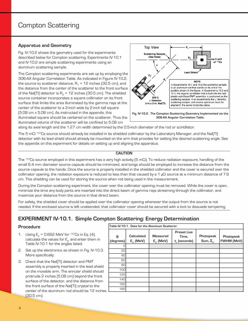
Fig. IV-10.2 shows the geometry used for the experiments

described below for Compton scattering. Experiments IV-10.1

and IV-10.2 are simple scattering experiments using an

aluminum scattering sample.

The Compton scattering experiments are set up by employing the

306-AX Angular Correlation Table. As indicated in Figure IV-10.2,

the source to scatterer distance, R1 = 12 inches (30.5 cm), and

the distance from the center of the scatterer to the front surface

of the NaI(Tl) detector is R2 = 12 inches (30.5 cm). The shielded

source container incorporates a square collimator on its front

surface that limits the area illuminated by the gamma rays at the

center of the scatterer to a 2-inch wide by 2-inch tall square

(5.08 cm x 5.08 cm). As instructed in the appendix, this

illuminated square should be centered on the scatterer. Thus the

illuminated volume of the scatterer will be confined to 5.08 cm

along its axial length and the 1.27 cm width determined by the 0.5-inch diameter of the rod or scintillator.

The 5 mCi 137Cs source should already be installed in its shielded collimator by the Laboratory Manager, and the NaI(Tl)

detector with its lead shield should already be mounted on the arm that provides for setting the desired scattering angle. See

the appendix on this experiment for details on setting up and aligning the apparatus.

CAUTION

The 137Cs source employed in this experiment has a very high activity (5 mCi). To reduce radiation exposure, handling of the

small 6.4 mm diameter source capsule should be minimized, and tongs should be employed to increase the distance from the

source capsule to the hands. Once the source is properly installed in the shielded collimator and the cover is secured over the

collimator opening, the radiation exposure is reduced to less than that caused by a 1 µCi source at a minimum distance of 7.6

cm. This shielding can be used for storing the source when not being used in the measurement.

During the Compton scattering experiment, the cover over the collimator opening must be removed. While the cover is open,

minimize the time any body parts are inserted into the direct beam of gamma rays streaming through the collimator, and

maximize your distance from the source in that direct beam.

For safety, the shielded cover should be applied over the collimator opening whenever the output from the source is not

needed. If the enclosed source is left unattended, that collimator cover should be secured with a lock to dissuade tampering.

EXPERIMENT IV-10.1. Simple Compton Scattering: Energy Determination

Procedure

1. Using Eγ = 0.662 MeV for 137Cs in Eq. (4),

calculate the values for Eγ’ and enter them inTable IV-10.1 for the angles listed.

2. Set up the electronics as shown in Fig. IV-10.3.

More specifically:

3. Check that the NaI(Tl) detector and PMT

assembly is properly inserted in the lead shield

on the movable arm. The annular shield should

protrude 2 inches (5.08 cm) beyond the front

surface of the detector, and the distance from

the front surface of the NaI(Tl) crystal to the

center of the aluminum rod should be 12 inches

(30.5 cm).

Fig. IV-10.2. The Compton Scattering Geometry Implemented via the

306-AX Angular Correlation Table.

Table IV-10.1. Data for the Aluminum Scatterer.

θ(degrees)

Calculated

Eγ’ (MeV)

Measured

Eγ’ (MeV)

Preset Live

Time,

tL (seconds)

Photopeak

Sum, Σγ’

Photopeak

FWHM (MeV)

0

20

40

60

80

100

120

140

160

180

5

Compton Scattering

4. Verify that the 5 mCi 137Cs source in its shield is properly mounted with the source positioned 12 inches (30.5 cm) from

the center of the aluminum scatterer. The location of the source in the shield is marked on the outside of the shield

(10.2 cm behind the front, outside surface of the collimator). Ensure that the cover shield is in place over the source

collimator to shut off the output of 662 keV gamma rays.

IV-10.1.1. Energy Calibration

The system should already be cabled correctly. A single USB

cable between the digiBASE and the PC is all that is required.

If the software is installed correctly,

then starting the MAESTRO program

“MAESTRO for Windows” should result

in the main MAESTRO screen

appearing (Fig. IV-10.5).

If the screen shows “Buffer” in block 4

(Fig. IV-10.6), then the software has

been unable to “find” the digiBASE and

assistance should be sought, or the

MAESTRO manual referred to.

Assuming that the legend in the box reads “digibase”,

communication is established.

1. Under the MAESTRO menu item “Acquire” select “MCB

Properties”.

The MCB properties for the digiBASE will look similar to Fig. IV-10.7 The tabs

provide access to the controlling functions of the digiBASE.

2. Ensure that the NaI(Tl) detector assembly is properly mounted in the stand.

3. There are two parameters that ultimately determine the overall gain of the system:

the high voltage furnished to the PMT and the gain of the spectroscopy amplifier.

The gain of the PMT is quite dependent upon its high voltage. A rule of thumb for

most PMTs is that, near the desired operating voltage, a 10% change in the high

voltage will change the gain by a factor of 2.

4. The correct high voltage value depends on the PMT being used. Consult your

instruction manual for the PMT and select a value in the middle of its normal

operating range. Sometimes, the detector will have a stick-on label that lists the percent resolution and the voltage at which

that resolution was measured. In that case, use the high voltage value on that label. Lacking those sources to specify the

operating voltage, check with the laboratory instructor for the recommended value.

The operating voltage will likely fall in the range of +800 to +1300 Volts.

Fig. IV-10.3. Generic Functional Block Diagram of Gamma-Ray

Spectroscopy System for Experiments IV-10.1 and IV-10.2. All of

these functions are incorporated within the digiBASE.

Fig. IV-10.4 digiBASE All-in-One

PMT Base, HV, Preamplifier,

Amplifier, and Digital MCA.

Fig. IV-10.5 Starting

MAESTRO.

Fig. IV-10.6 Main MAESTRO Screen.

Fig. IV-10.7 MCB Properties.

6

Compton Scattering

5. Select the High Voltage tab

6. Enter the detector high voltage in the Target field, click On, and monitor the voltage

in the Actual field.

7. On the Amplifier tab, choose a shaping time of 0.75 µS and a starting fine gain

setting of 0.5 and 0.5 respectively. (The coarse gain on the digiBASE is set by

Jumper, and should not need to be changed).

8. Using the ADC tab select a conversion gain of 1024 channels for the pulse-height

range of 0 to +10 Volts. Turn the GATE to Off. For a starting value, the lower level

discriminator threshold can be set to about 100 mV (10 channels). Set the upper

level discriminator to full scale (1023).

9. On the Presets tab set both real and live presets to Zero (“off”).

IV-10.1.2. A Note on Bipolar Filtering

Unlike many “Gaussian” spectroscopy amplifier filters which require so called “Pole-

Zero” cancellation, the Bipolar filter in the digiBASE requires no such adjustment. For

further discussion on amplifier filters see www.ortec-online.com/download/Amplifier-

Introduction.pdf

A representation of the digital bipolar waveform may be displayed through the use of

the “InSight” display mode selectable via the “Amplifier 2” tab. Remember to click the

“STOP” control on returning to the Amplifier 2 tab or you wll not be able to display the

gamma-ray spectrum!

IV-10.1.3. Adjusting the Gain for Recording Spectra (refer to Experiment

IV-3)

1. From the RSS8 Source Kit, select the 1 µCi 137Cs source and place it directly in front of

the NaI(Tl) detector.

2. Set the HV to the designated value. Adjust the amplifier coarse and fine gain until the

spectrum looks as in Fig. IV-10.11 Accelerator keys allow this adjustment to be made

while observing the spectrum:

ALT+ increases the gain one increment

ALT- decreases the gain one increment

SHIFT ALT + increases the gain several increments

SHIFT ALT – decreases the gain several increments

ALT 1 starts an acquisition

ALT 2 stops an acquisition

ALT 3 clears acquired or acquiring data

3. Acquire a spectrum with the digiBASE for at least 30

seconds, and no more than a couple of minutes. The

spectrum should look like Figure IV-10.11

4. Adjust the amplifier gain so that the 662 keV peak is located

at circa channel 400 during acquisition by the MCA.

Fig. IV-10.9 Presets Tab.

Fig. IV-10.10 Digital Polar Waveform.

Fig. IV-10.11 NaI(Tl) Spectrum for 137Cs.

Fig. IV-10.8 High Voltage Tab.

7

Compton Scattering

IV-3.1.4. Lower-Level Discriminator Adjustment

The optimum setting of the Lower-Level Discriminator threshold is slightly above the maximum noise amplitude. This prevents

the MCA from wasting time analyzing the useless information in the noise surrounding the baseline between valid pulses.

Setting the Lower-Level Discriminator threshold reasonably close to the noise improves the quality of the automatic dead time

correction by measuring the full duration of the pulses at the noise threshold. To adjust the Lower-Level Discriminator use the

following procedure.

1. Remove any radioactive sources from the vicinity of the NaI(Tl) detector, so that no gamma rays are being detected.

2. Start a data acquisition and observe the Percent Dead Time displayed for the MCA. It should be less than 1%. If the dead

time is larger than 1% jump to step 5.

3. Using the MCB Properties menu, reduce the Lower-Level Discriminator threshold, start another acquisition and observe

the percent dead time.

4. Keep repeating step 3 until the percent dead time abruptly increases.

5. Once the dead time increases significantly above 1%, gradually increase the Lower-Level Discriminator threshold until the

percent dead time is less than 1%.

6. Repeat steps 3 through 5 until you are confident the threshold has been set reasonably close to the noise, with little risk

of counting random noise excursions.

The absolute amplitude of the noise at the MCA input is dependent on the preamplifier characteristics and the gain setting on

the amplifier. Consequently, the MCA Lower-Level Discriminator

threshold should be adjusted any time the amplifier gain is

changed, or the preamplifier is replaced with a different unit.

Adjustment of this threshold is important whenever a detector

system is assembled for initial set-up.

7. Remove the 1 µCi 137Cs source and acquire a spectrum.

Ensure that the MCA is not acquiring significant noise events

near channel 10. If the noise is accumulating at a noticeable

counting rate and the MCA dead time is >1%, raise the lower

level discriminator setting until the noise is no longer observed.

8. Select the appropriate sources from the RSS8 source kit and

calibrate the digiBASE so that its cursor reads the correct

energy of the photopeaks. Table IV-10.2 lists the gamma-ray

energies for the isotopes in the source kit.

9. Remove the energy-calibration sources. Install the aluminum

rod vertically in the scattering position at the center of the

table. Next, remove the cover shield from the collimator on the

5 mCi 137Cs source enclosure.

10. Position the NaI(Tl) detector at θ = 60°. This is the position atwhich the lowest counting rate will be recorded. Set the preset

live time on the digiBASE at 100 seconds, and acquire a

spectrum for that live time.

11. Set a Region of Interest (ROI) across the entire photopeak

from the valley on the lower energy side to the baseline on the

higher energy side. Sum the counts in the photopeak using the

ROI integration feature of the MAESTRO software. Read the

“Net Area” which reports the area above any background

under the peak. The background should be negligible.

Table IV-10.2. Gamma- and X-ray Energies from the RSS8 Source Kit.

Isotope Half Life

X-ray

Series

X-ray

Energies (keV)

Gamma-Ray

Energies (keV)

22Na 950.8d 511

1275

54Mn 312.3d Cr K 5.414 835

5.405

5.946

57Co 271.79 d Fe K 6.403 14

6.390 122

7.057 136.5

60Co 5.272 y 1173

1333

65Zn 244.26 d Cu K 8.047 1116

8.027

8.904

8.976

109Cd 462.6 d Ag K 22.162 88

21.988

24.942

25.454

133Ba 3862 d Cs K 30.970 80

30.623 303

34.984 356

35.819

137Cs 30.17 y Ba K 32.191 662

31.815

36.376

37.255

8

12. From the result in step 11, determine the preset live time necessary to accumulate at least 1,000 net counts in the

photopeak. Use this preset live time for acquiring the spectra at each of the angles in Table IV-10.1. Note that the

spectrum will not be measured at 0° because of an excessive counting rate from the unscattered radiation from the

source. No measurement will be made at 180° because the lead shields make that angle inaccessible.

13. For each of the angles in Table IV-10.1 (except 0° and 180°), acquire a spectrum for the preset live time determined in

step 12. In each case, set an ROI across the photopeak as described

in step 11. Using the MAESTRO features, measure the peak position

(centroid) and the net area of the peak. Record those numbers in the

3rd and 5th columns of Table IV-10.1. Measure the FWHM of each

photopeak and record that value in Table IV-10.1. You may wish to

save a copy of each spectrum on the hard disk, in case you find a

reason later to re-examine the raw data. As predicted by equation (4),

the photopeak energy will decrease as θ increases. Figure IV-10.12shows an example of two spectra obtained at 20° and 120°, but at

twice the conversion gain called for in step 11.

14. At the completion of the measurements, replace the shield over the

source collimator opening to shut off the flux of gamma rays.

EXERCISES

a. Plot the Eγ’ values calculated from Equation (4) versus θ on linear graph paper. Add your measured values of Eγ’ togetherwith ±1-sigma error bars from equation (6). Explain the reasons for any discrepancies between the theoretical and

measured values for Eγ’.

b. Plot your measured values of 1/Eγ’ versus (1 – cosθ) on a linear graph. Equation (6) gives the predicted standard

deviation in the measured Eγ’. Convert that standard deviation into the corresponding error for 1/Eγ’, and add theappropriate error bars to your points on the graph. Draw a best fit straight line through your measured points. Read the

slope of the straight line and its intercept from the graph. Explain any discrepancy between those graphical values and the

prediction from equation (5b). Your graph should look similar to Figure IV-10.13.

Compton Scattering

Fig. IV-10.12. Overlapped Spectra Obtained at Two

Scattering Angles.

Fig. IV-10.13. A Typical Graph for 1/Eγ’ versus (1 – cosθ) for137Cs.

Table IV-10.3. Typical Tabulated Values

for Equation (5b) and Fig. IV-10.13.

Angle (θ) 1/Eγ’ (MeV–1) 1 – cosθ

0 1.51 0

10 1.54 0.015

20 1.63 0.060

30 1.77 0.133

40 1.97 0.234

50 2.20 0.357

60 2.49 0.500

70 2.79 0.658

80 3.12 0.826

90 3.46 1.00

100 3.80 1.17

110 4.13 1.34

120 4.44 1.50

130 4.72 1.64

9

Compton Scattering

EXPERIMENT IV-10.2. Simple Compton Scattering: Cross-Section Determination

Purpose

The data collected in Experiment IV-10.1 will be used to calculate the measured scattering cross-section and compare it to

the theoretical cross-section.

Relevant Information

Theoretical Differential Cross-Section

The differential cross-section for Compton scattering, first proposed by Klein and Nishina, is discussed in ref. 1. The

theoretical expression for unpolarized gamma rays has the following form:

dσ r 20 1 + cos2θ α2(1 – cosθ)2

––––= ––––{–––––––––––––––––––––}{1 + –––––––––––––––––––––––––––––––––} (7a)dΩ 2 [1 + α(1 – cosθ)]2 [1 + cos2θ][1 + α(1 – cosθ)]

Equation (7a) is the differential cross-section for scattering from a single electron, and is expressed in units of cm2/steradian.

It represents the effective differential area, dσ, of the electron as a target for scattering the gamma-ray photon at the angle θinto an infinitessimal solid angle, dΩ. The new parameters in equation (7a) are the classical electron radius

r0 = 2.82 x 10–11 cm (7b)

And the normalized (dimensionless) energy

Eγ 0.662 MeVα = ––––––= ––––––––––––––= 1.296 for 137Cs (7c)

m0c2 0.511 MeV

Experimentally Measured Differential Cross-Section

The data already collected in Experiment IV-10.1 can be used to calculate the measured differential scattering cross-section

by employing equation (8).

dσ Σγ’[––––] = ––––––––––––– (8a)dΩ measured ne I ΔΩ tL ε

Where ne is the number of electrons in the portion of the scatterer illuminated by the incident gamma rays. For a scatterer

composed of multiple elements, ne can be calculated from the basic parameters for the material, i.e.,

Zine = ρ V NA wi –––– (8b)Σ

Mii

Where:

ρ is the density of the scatterer in g/cm3,V is the volume (in cm3) of the scatterer that is illuminated by the incident gamma rays,

NA is Avogadro’s Number (6.022 x 1023),

Zi is the atomic number of the ith element in the scatterer,

Mi is the gram atomic weight of the ith element in the scatterer, and

wi is the concentration of the ith element in the scatterer, expressed as a weight fraction.

By definition, the weight fractions for all elements in the scatterer sum to unity.

wi = 1 (8c)Σi

10

Compton Scattering

The variable, I, is the number of incident gamma rays per cm2 per second at the scattering sample. It can be calculated from

A0fI = –––––– (8d)

4πR21

Where A0 is the activity of the source (5 mCi), f is the fraction of the decays that result in the emission of 662 keV gamma-

rays (0.851) and R1 is the distance from the source to the center of the scatterer.

The solid angle subtended by the NaI(Tl) detector at the scatterer is computed from

D 2

π(––)2

ΔΩ = ––––––– (8e)R2

2

Where D = 5.08 cm is the diameter of the NaI(Tl) scintillation

crystal, and R2 is the distance from the center of the

scatterer to the front surface of the NaI(Tl) detector.

Σγ’ is the total number of counts in the photopeak for thescattered gamma ray acquired during the live time, tL. The

intrinsic photopeak efficiency, є, can be obtained fromFig. IV-10.14.

Note that Figure IV-10.14 differs from the virtually identical

graph in Experiment 3. There were no measured values at

0.124 MeV in the original graph for the 2” x 2” and 3” x 3”

detector sizes. For the purposes of Experiment IV-10, these

points have been interpolated between є = 1.00 and themeasured value on the 1.5” x 1.5” curve. Although adequate

for this experiment, the interpolated values are not reliable

for more general use.

For convenience, the elemental composition for the aluminum

rod alloy is listed in Table IV-10.4. According to the ASTM

standard, the composition can vary over the range in

columns 2 and 3. For the purposes of this experiment, the

mean of the maximum and minimum concentrations has

been tabulated in column 4. The calculation in equation (8b)

can be simplified further by ignoring elements with concentrations

<0.6%. That approximation would elevate the Al concentration to

98.4%. Note that the weight fraction used in equation (8b) is simply the

percent concentration divided by 100%.

Procedure

The data for this experiment has already been measured and recorded

in Experiment IV-10.1.

Fig. IV-10.14. The Intrinsic Photopeak Efficiency, є, for Three Sizes ofNaI(Tl) Detectors. CAVEAT: The points for 0.124 MeV on the 2” x 2” and 3”

x 3” lines are interpolated between 1.00 and the measured value for the

1.5” x 1.5” curve.

Table IV-10.4. The Composition of the Aluminum Scatterer.

ASTM Aluminum Alloy 606-T651

Density = 2.7 g/cm3

Element Min. Weight % Max. Weight %

Nominal (Mean)

Weight %

Al 95.8 98.6 97.23

Mg 0.8 1.2 1.00

Si 0.4 0.8 0.60

Fe 0.7 0.35

Cu 0.15 0.4 0.25

Cr 0.04 0.35 0.20

Zn 0.25 0.13

Mn 0.15 0.08

Ti 0.15 0.08

Other 0.15 0.08

11

Compton Scattering

EXERCISES

a. Compute dσ/dΩ from Eq. (7) for the values of θ used in Table IV-10.1. (A spreadsheet is quite valuable for this

calculation, although not absolutely necessary).

b. Plot the theoretical dσ/dΩ versus θ on a linear graph.

c. Use the data measured in Experiment IV-10.1 with equations (8) to calculate [dσ/dΩ]measured, and plot your measured

values on the graph from step b.

d. Estimate the standard deviation in your measured values based on counting statistics. Add the error bars to the points on

the graph in step c to represent the ±1-sigma predicted errors.

e. Discuss possible reasons for any discrepancies between the theoretical and measured differential cross-sections.

References

1. A.C. Melissinos, Experiments in Modern Physics, Academic Press, New York (1966).

2. G. F. Knoll, Radiation Detection and Measurement, John Wiley and Sons, Inc., New York (1979).

3. P. Quittner, Gamma Ray Spectroscopy, Halsted Press, New York (1972).

4. W. Mann and S. Garfinkel, Radioactivity and Its Measurement, Van Nostrand-Reinhold, New York (1966).

5. K. Siegbahn, Ed., Alpha-, Beta-, and Gamma-Ray Spectroscopy, 1, North Holland Publishing Co., Amsterdam (1965).

6. C. M. Lederer and V. S. Shirley, Eds., Table of Isotopes, 7th Edition, John Wiley and Sons, Inc., New York (1978).

7. R. L. Heath, "Scintillation Spectrometry", Gamma-Ray Spectrum Catalog, 2nd Edition 1 and 2, IDO 16880, August, (1964).

Available from Clearinghouse for Federal Scientific and Technical Information, Springfield, Virginia. Electronic copy

available at http://www.inl.gov/gammaray/catalogs/catalogs.shtml.

8. G. Marion and P. C. Young, Tables of Nuclear Reaction Graphs, John Wiley and Sons, Inc., New York (1968).

9. D. A. Gedcke, How Histogramming and Counting Statistics Affect Peak Position Precision, ORTEC Application Note AN58,

(2005), http://www.ortec-online.com/Library/index.aspx.

APPENDIX IV-10-A: Installing the 5 mCi 137Cs Source in the Shielded Collimator and

Checking Alignment

Installing the Source in the Shielded Enclosure

The shielded collimator enclosure and the 5 mCi 137Cs radioactive source are shipped separately from their manufacturers.

Installation of the source into the shielded collimator needs to be implemented by the Laboratory Manager prior to use in any

experiments. Observe the above caution about handling this high-activity source. Use the following procedure for installing the

source.

1. Remove the cover shield that is secured over the collimator window.

2. Remove any screws that are retaining the front of the collimator section to the main body of the enclosure.

3. Withdraw the collimator and the attached tube from the well in the enclosure.

4. At the end of the tube that is remote from the square collimator window, there is a hole drilled in the circular end-plate

along the center line of the tube. The diameter of this hole is slightly larger than 0.25 inches (6.35 mm), and accepts the

similar outer diameter of the source capsule.

Tel. (865) 482-4411 • Fax (865) 483-0396 • ortec.info@ametek.com

801 South Illinois Ave., Oak Ridge, TN 37830 U.S.A.

For International Office Locations, Visit Our Website

www.ortec-online.comORTEC ®

Specifications subject to change

071515

Compton Scattering

5. Loosen the clamp at the entrance to this hole, and insert the source capsule with its active end towards the collimator

window. Make sure the source capsule is inserted until it is stopped by the lip at the end of the hole. The lip ensures the

proper insertion depth.

6. Tighten the clamp so that the source capsule cannot move from its proper position.

7. Insert the source, tube and collimator assembly into the well in the shielded enclosure.

8. Reinstall the retaining screw(s) to hold the collimator/source assembly in the shielded enclosure.

9. Place the shielded cover over the collimator opening, and secure it with a lock and key.

10. Using a radiation dosimeter capable of reading exposure rates as low as 0.1 mR/hr. with gamma-ray energies in the

range of 100 to 662 keV, survey the entire outside of the enclosure to determine the exposure rate at the surface of the

enclosure. Verify that there are no intolerable exposure rates from gaps in the shielding.

11. When not employed in the experiment, store the source and enclosure in a secure location.

Checking Alignment in the Compton Scattering Experiment

The mechanical keying features on the Angular Correlation Table and the 5 mCi 137Cs source enclosure/collimator should

provide proper alignment for the Compton Scattering Experiment. The centerline of the source collimator and the centerline of

the NaI(Tl) detector should lie in the same scattering plane. Where that plane intersects the vertical centerline of the

aluminum scattering rod or the plastic scintillator rod defines the desired center of the collimated gamma-ray beam at the

scatterer. The collimated gamma-ray beam should extend ±1 inch (±2.54 cm) in the vertical direction around that centerline.

The beam should also extend ±1 inch (±2.54 cm) in the horizontal plane with respect to the vertical centerline of the

scattering rod.

This alignment can be checked using the plastic scintillator. To measure the horizontal limits of the gamma-ray beam, move

the plastic scintillator horizontally across the beam while monitoring the counting rate. To measure the vertical extent of the

gamma-ray beam, use the plastic scintillator with its long axis in the horizontal plane, and scan in the vertical direction, while

monitoring the counting rate. The distance resolution with this method will be approximately determined by the diameter of

the plastic scintillator.