an overview on assessing agreement with...
TRANSCRIPT
An Overview On Assessing Agreement With
Continuous Measurement
Huiman X. Barnhart
Department of Biostatistics and Bioinformatics
and Duke Clinical Research Institute
Duke University
PO Box 17969
Durham, NC 27715
Tel: 919-668-8403
Fax: 919-668-7049
Michael J. Haber
Department of Biostatistics
The Rollins School of Public Health
Emory University
Atlanta, GA 30322
Lawrence I. Lin
Baxter Healthcare Inc.
Round Lake, IL 60073
Lawrence [email protected]
Corresponding Author: Huiman X. Barnhart
1
ABSTRACT
Reliable and accurate measurements serve as the basis for evaluation in many scientific
disciplines. Issues related to reliable and accurate measurement have evolved over many
decades, dating back to the 19th century and the pioneering work of Galton (1886), Pearson
(1896, 1899, 1901) and Fisher (1925). Requiring a new measurement to be identical to
the truth is often impractical, either because (1) we are willing to accept a measurement
up to some tolerable(or acceptable) error, or (2) the truth is simply not available to us,
either because it is not measurable or is only measurable with some degree of error. To
deal with issues related to both (1) and (2), a number of concepts, methods, and theories
have been developed in various disciplines. Some of these concepts have been used across
disciplines, while others have been limited to a particular field but may have potential
uses in other disciplines. In this paper, we elucidate and contrast fundamental concepts
employed in different disciplines and unite these concepts into one common theme: assessing
closeness (agreement) of observations. We focus on assessing agreement with continuous
measurement and classify different statistical approaches as (1) descriptive tools; (2) unscaled
summary indices based on absolute differences of measurements; and (3) scaled summary
indices attaining values between -1 and 1 for various data structures, and for cases with and
without a reference. We also identify gaps that require further research and discuss future
directions in assessing agreement.
Keywords: Agreement; Limits of Agreement; Method Comparison; Accuracy; Precision;
Repeatability; Reproducibility; Validity; Reliability; Intraclass Correlation Coefficient; Gen-
eralizability; Concordance Correlation Coefficient; Coverage Probability; Total Deviation
Index; Coefficient of Individual Agreement; Tolerance Interval.
1 Introduction
In social, behavioral, physical, biological, and medical sciences, reliable and accurate mea-
surements serve as the basis for evaluation. As new concepts, theories, and technologies
continue to develop, new scales, methods, tests, assays, devices, and instruments for evalu-
2

ation become available for measurement. Because errors are inherent in every measurement
procedure, one must ensure that the measurement is reliable and accurate before it is used
in practice. The issues related to reliable and accurate measurement have evolved over many
decades, dating back to the 19th century and the pioneering work of Galton (1886), Pearson
(1896, 1899, 1901) and Fisher (1925): from the intraclass correlation coefficient (ICC) that
measures reliability (Galton, 1886; Pearson, 1896; Fisher, 1925; Bartko, 1966, Shrout and
Fleiss, 1979; Vangeneugden et al., 2004) and the design of reliability studies (Donner, 1998;
Dunn, 2002; Shoukri et al., 2004), to generalizability extending the concept of ICC (Cron-
back, 1951; Lord and Novick, 1968; Cronback et al.,1972; Brennan, 2001; Vangeneugden et
al., 2005); from the International Organization for Standardizations (ISO) (1994) guiding
principle on accuracy of measurement (ISO 5725-1) to the Food and Drug Administrations
(FDA) (2001) guidelines on bioanalytical method validation; and including various indices to
assess the closeness (agreement) of observations (Bland and Altman, 1986, 1995, 1999; Lin,
1989, 2000, 2003; Lin et al., 2002; Shrout, 1998; King and Chinchilli, 2001a; Dunn, 2004;
Carrasco and Jover, 2003a; Choudhary and Nagaraja, 2004; Barnhart et al., 2002, 2005a;
Haber and Barnhart, 2006).
In the simplest intuitive terms, reliable and accurate measurement may simply mean that
the new measurement is the same as the truth or agrees with the truth. However, requiring
the new measurement to be identical to the truth is often impractical, either because (1)
we are willing to accept a measurement up to some tolerable (or acceptable) error or (2)
the truth is simply not available to us (either because it is not measurable or because it is
only measurable with some degree of error). To deal with issues related to both (1) and (2),
a number of concepts, methods, and theories have been developed in different disciplines.
For continuous measurement, the related concepts are accuracy, precision, repeatability,
reproducibility, validity, reliability, generalizability, agreement, etc. Some of these concepts
(e.g., reliability) have been used across different disciplines. However, other concepts, such as
generalizability and agreement, have been limited to a particular field but may have potential
uses in other disciplines.
In this paper, we describe and contrast the fundamental concepts used in different dis-
ciplines and unite these concepts into one common theme: assessing closeness (agreement)
3

of observations. We focus on continuous measurements and summarize methodological ap-
proaches for expressing these concepts and methods mathematically, and discuss the data
structures for which they are to be used, both for cases with and without a reference (or
truth). Existing approaches for expressing agreement are organized in terms of the following:
(1) descriptive tools, such as pairwise plots with a 45-degree line and Bland and Altman plots
(Bland and Altman, 1986); (2) unscaled summary indices based on absolute differences of
measurements, such as mean squared deviation including repeatability coefficient and repro-
ducibility coefficient, limits of agreement (Bland and Altman, 1999), coverage probability,
and total deviation index (Lin et al., 2002); and (3) scaled summary indices attaining val-
ues between -1 and 1, such as the intraclass correlation coefficient, concordance correlation
coefficient, coefficient of individual agreement, and dependability coefficient.
These approaches were developed for one or more types of the following data structure:
(1) two or more observers without replications; (2) two or more observers with replications;
(3) one or more observer is treated as a random or fixed reference; (4) longitudinal data
where observers take measurements over time; (5) data where covariates are available for
assessing the impact of various factors on agreement measures. We discuss the interpretation
of the magnitude of the agreement values on using the measurements in clinical practice and
on study design of clinical trials. We also identify gaps that require further research, and
discuss future directions in assessing agreement. In Section 2, we present definitions of
different concepts used in the literature and provide our critique. Statistical approaches are
presented in Section 3 where various concepts are used. We conclude with a summary and
discussions of future directions in Section 4.
2 Concepts
2.1 Accuracy and Precision
In Merriam Webster’s dictionary, accuracy and precision are synonyms. Accuracy is defined
as “freedom from mistake or error” or “conformity to truth or to a standard” or “degree of
conformity of a measure to a standard or a true value.” Precision is defined as “the quality of
being exactly or sharply defined” or “the degree of refinement with which a measurement is
4

stated.” The “degree of conformity” and “degree of refinement” may mean the same thing.
The subtle difference between these two terms may lie in whether a truth or a reference
standard is required or not.
Accuracy
Historically, accuracy has been used to measure systematic bias while precision has been
used to measure random error around the expected value. Confusion regarding the use of
these two terms continues today because of the existence of different definitions and because
of the fact that these two terms are sometimes used interchangeably. For example, the U.S.
Food and Drug Administration (FDA) guidelines on bioanalytical method validation (1999)
defined accuracy as the closeness of mean test results obtained by the method to the true value
(concentration) of the analyte. The deviation of the mean from the true value, i.e., systematic
bias, serves as the measure of accuracy. However, in 1994, the International Organization for
Standardization (ISO) used accuracy to measure both systematic bias (trurness) and random
error. In ISO 5725 (1994), the general term accuracy was used to refer to both trueness and
precision, where“trueness” refers to the closeness of agreement between the arithmetic mean
of a large number of test results and the true or accepted reference value, and “precision”
refers to the closeness of agreement between test results. In other words, accuracy involves
both systematic bias and random error, because “trueness” measures systematic bias. The
ISO 5725 (1994) acknowledged that:
“The term accuracy was at one time used to cover only the one component now named
trueness, but it became clear that to many persons it should imply the total displacement of a
result from a reference value, due to random as well as systematic effects. The term bias has
been in use for statistical matters for a very long time, but because it caused certain philosoph-
ical objections among members of some professions (such as medical and legal practioners),
the positive aspect has been emphasized by the invention of the term “trueness””.
Despite the ISO’s effort to use one term (accuracy) to measure both systematic and
random errors, the use of accuracy for measuring the systematic bias, and precision for
measuring random error, is commonly encountered in the literature of medical and statistical
research. For this reason, we will use accuracy to stand for systematic bias in this paper,
where one has a “true sense of accuracy” (systematic shift from truth) if there is a reference,
5

and a “loose sense of accuracy” (systematic shift from each other) if no reference is used
for comparison. Thus, the “true sense of accuracy” used in this paper corresponds to the
FDA’s accuracy definition and the ISO’s trueness definition. Ideally and intuitively, the
accepted reference value should be the true value, because one can imagine that the true
value has always existed, and the true value should be used to judge whether there is an
error. However, in social and behavioral sciences, the true value may be an abstract concept,
such as intelligence, which may only exist in theory and may thus not be amenable to direct
measurement. In biomedical sciences, the true value may be measured with a so- called gold
standard that may also contain small amount of systematic and/or random error. Therefore,
it is very important to report the accepted reference, whether it is the truth or subject to
error (including the degree of systematic and random error if known). In this paper, we only
consider the case where the reference or gold standard is measured with error.
Precision
The FDA (1999) defined precision as the closeness of agreement (degree of scatter) be-
tween a series of measurements obtained from multiple sampling of the same homogeneous
sample under the prescribed conditions. Precision is further subdivided into within-run,
intra-batch precision or repeatability (which assesses precision during a single analytical
run) and between-run, inter-batch precision or repeatability (which measures precision over
time, and may involve different analysts, equipment, reagents, and laboratories).
ISO 5725 (1994) defined precision as the closeness of agreement between independent test
results obtained under stipulated conditions. ISO defined repeatability and reproducibility
as precision under the repeatability and reproducibility conditions, respectively (see Section
2.2).
The key phrase is “under the prescribed conditions” or “under stipulated conditions.” It
is therefore important to emphasize the conditions used when reporting precision. Precisions
are only comparable under the same conditions.
2.2 Repeatability and Reproducibility
Repeatability and reproducibility are two special kinds of precision under two extreme condi-
tions and they should not be used interchangeably. As defined below, repeatability assesses
6
pure random error due to “true” replications and reproducibility assesses closeness between
observations made under condition other than pure replication, e.g., by different labs or ob-
servers. If precision is expressed by imprecision such as standard deviation, repeatability is
always smaller than or equal to reproducibility (see below for definition).
Repeatability
The FDA (2001) used the term repeatability for both intra-batch precision and inter-batch
precision. The ISO defined repeatability as the closeness of agreement between independent
test results under repeatability conditions that are as constant as possible, where indepen-
dent test results are obtained with the same methods, on identical test items, in the same
laboratory, performed by the same operator, using the same equipment, within short intervals
of time.
We use the ISO’s definition of repeatability in this paper. To define the term more
broadly, repeatability is the closeness of agreement between measures under the same con-
dition, where “same condition” means that nothing changed other than the times of the
measurements. The measurements taken under the same condition can be viewed as true
replicates.
Sometimes the subject does not change over time, as in the case of x-ray slides or blood
samples. However, in practice, it may be difficult to maintain the same condition over time
when measurements are taken. This is especially true in the social and behavioral sciences,
where characteristics or constructs change over time due to learning effects. It is important
to ensure that human observers are blinded to earlier measurements of the same quantity.
We frequently rely on believable assumptions that the same condition is maintained over a
short period of time when measurements are taken. It is essential to state what assumptions
are used when reporting repeatability. For example, when an observer uses an instrument to
measure a subject’s blood pressure, the same condition means the same observer using the
same instrument to measure the same subject’s blood pressure, where the subject’s blood
pressure did not change over the course of multiple measurements. It is unlikely that the
subject’s blood pressure remains constant over time; however, it is believable that the true
blood pressure did not change over a short period time, e.g., a few seconds. Therefore, blood
pressures taken in successive seconds by the same observers, using the same instrument on
7

the same subject, may be considered true replicates.
It is important to report repeatability when assessing measurement, because it measures
the purest random error that is not influenced by any other factors. If true replicates cannot
be obtained, then we have a loose sense of repeatability based on assumptions.
Reproducibility
In 2001, FDA guidelines defined reproducibility as the precision between two laboratories.
Repeatability also represents the precision of the method under the same operating conditions
over a short period of time. In 1994, the ISO defined reproducibility as the closeness of
agreement between independent test results under reproducibility conditions under which
results are obtained with the same method on identical test items, but in different laboratories
with different operators and using different equipment.
We use the ISO’s definition of reproducibility in this paper. To define the term more
broadly, reproducibility is the closeness of agreement between measures under all possible
conditions on identical subjects for which measurements are taken. All possible conditions
means any conceivable situation for which a measurement will be taken in practice, including
different laboratories, different observers, etc. However, if multiple measurements on the
same subject cannot be taken at the same time, one must ensure that the thing being
measured (e.g, a subject’s blood pressure) does not change over time when measurements
are taken in order to assess reproducibility.
2.3 Validity and Reliability
The concepts of accuracy and precision originated in the physical sciences, where direct
measurements are possible. The similar concepts of validity and reliability are used in the
social sciences, where a reference is required for validity but not necessarily required for
reliability. As elaborated below, validity is similar to true sense of agreement with both
good true sense of accuracy and precision. Reliability is similar to loose sense of agreement
with both good loose sense of accuracy and precision. Historically, validity and reliability
have been assessed via scaled indices.
Validity
In social, educational, and psychological testing, validity refers to the degree to which evi-
8

dence and theory support the interpretation of measurement (AERA et al., 1999). Depending
on the selection of the accepted reference (criterion or gold standard), there are several types
of validity such as content, construct, criterion validity (Goodwin, 1997; AERA et al., 1999;
Kraemer et al., 2002; Hand, 2004; Molenberghs, et al., 2007). Content validity is defined
as the extent to which the measurement method assesses all the important content. Face
validity is similar to content validity, and is defined as the extent to which the measure-
ment method assesses the desired content at face. Face validity may be determined by the
judgment of experts in the field. Construct validity is used when attempting to measure a
hypothetical construct that may not be readily observed, such as anxiety. Convergent and
discriminant validity may be used to assess construct validity by showing that the new mea-
surement is correlated with other measurements of the same construct and that the proposed
measurement is not correlated with the unrelated construct, respectively. Criterion validity
is further divided into concurrent and predictive validity, where criterion validity deals with
correlation of the new measurement with a criterion measurement (such as a gold standard)
and predictive validity deals with the correlation of the new measurement with a future
criterion, such as a clinical endpoint.
Validity is historically assessed by the correlation coefficient between the new measure
and the reference (or construct). If there is no systematic shift of the new measurement
from the reference or construct, this correlation may be expressed as the proportion of the
observed variance that reflects variance in the construct that the instrument or method
was intended to measure (Kraemer et al., 2002). For validation of bioanalytical methods,
the FDA (2001) provided guidelines on full validation that involve parameters such as (1)
accuracy, (2) precision, (3)selectivity, (4) sensitivity, (5) reproducibility, and (6) stability,
when a reference is available. The parameters related to selectivity, sensitivity and stability
may only be applicable in bioanalytical method. When the type of validity is concerned
with the closeness (agreement) of the new measurement and the reference, we believe that
an agreement index is better suited than the correlation coefficient for assessing validity.
Therefore, a statistical approach for assessing agreement for the case with a reference in
Section 3 can be used for assessing validity. Other validity measures that are based on a
specific theoretical framework and are not concerned with closeness of observations will not
9
be discussed in Section 3.
Reliability
The concept of reliability has evolved over several decades. It was initially developed in
social, behavioral, educational, and psychological disciplines, and was later widely used in
the physical, biological, and medical sciences (Fisher, 1925; Bartko, 1966, Lord and Novick,
1968; Shrout and Fleiss, 1979; Muller and Buttner, 1994; McGraw and Wong, 1996; Shrout,
1998; Donner, 1998; Shoukri et al., 2004; Vangeneugden et al., 2004). Rather than reviewing
the entire body of literature, we provide our point of view on its development. Reliability
was originally defined as the ratio of true score variance to the observed total score variance
in classical test theory (Lord and Novick, 1968; Cronbach et al., 1972), and is interpreted
as the percent of observed variance explained by the true score variance. It was initially
intended to assess the measurement error if an observer takes a measurement repeatedly on
the same subject under identical conditions, or to measure the consistency of two readings
obtained by two different instruments on the same subject under identical conditions. If the
true score is the construct, then reliability is similar to the criterion validity. In practice, the
true score is usually not available, and in this case, reliability represents the scaled precision.
Reliability is often defined with additional assumptions. The following three assumptions
are inherently used and are not usually stated when reporting reliability.
(a) The true score exists but is not directly measurable
(b) The measurement is the sum of the true score and a random error, where random errors
have mean zero and are uncorrelated with each other and with the true score (both
within and across subjects).
(c) Any two measurements for the same subject are parallel measurements.
In this context, parallel measurements are any two measurements for the same subject that
have the same means and variances. With assumptions (a) and (b), reliability, defined above
as the ratio of variances, is equivalent to the square of the correlation coefficient between the
observed reading and the true score. With assumptions (a) through (c), reliability, as defined
above, is equivalent to the correlation of any two measurements on the same subject. This
correlation is called intraclass correlation (ICC) and was originally defined by Galton (1889)
10

as the ratio of fraternal regression, a correlation between measurements from the same class
(in this case, brothers) in study of fraternal resemblance in genetics. Estimations of this ICC
based on sample moment (Pearson, 1896, 1899, 1901) and on variance components (Fisher,
1925) were later proposed. Parallel readings are considered to come from the same class
and can be represented by a one-way ANOVA model (see Section 3). Reliability expressed
in terms of ICC is the most common parameter used across different disciplines. Different
versions of ICC used for assessing reliability have been advocated (Bartko, 1966; Shrout and
Fleiss, 1979; Muller and Buttner, 1994; Eliasziw, et al., 1994; McGraw and Wong, 1996)
when different ANOVA models are used in place of assumptions (b) and (c). We discuss
these versions in Section 3.
2.4 Dependability and Generalizability
The recognition that assumptions (b) and (c) in classical test theory are too simplistic
prompted the development of generalizability theory (GT) (Cronbach et al., 1972; Shavelson
et al., 1989; Shavelson and Webb, 1981, 1991, 1992; Brennan, 1992, 2000, 2001). GT is
widely known and is used in educational and psychological testing literature; however, it
is barely used in medical research despite many efforts to encourage broader use since its
introduction by Cronbach et al. (1972).This may be due to the overwhelming statistical
concepts involved in the theory and the limited number of statisticians who have worked in
this area. Recently, Vangeneugden et al. (2005) and Molenberghs et al. (2007) presented
linear mixed model approaches to estimating reliability and generalizability in the setting of
a clinical trial.
GT extends classical test theory by decomposing the error term into multiple sources
of measurement errors, thus relaxing the assumption of parallel readings. The concept
of reliability is then extended to the general concept of generalizability or dependability
within the context of GT. In general, two studies (G-study and D-study) are involved,
with the G-study aimed at estimating the magnitudes of variances due to multiple sources of
variability through an ANOVA model, and the D-study, which uses some or all of the sources
of variability from the G-study to define specific coefficients that generalize the reliability
coefficient, depending on the intended decisions. In order to specify a G-study, the researcher
11

must define the universe of generalizability a priori. The universe of generalizability contains
factors with several levels/conditions (finite or infinite) so that researchers can establish the
interchangeability of these levels. For example, suppose there are J observers and a researcher
wants to know whether the J observers are interchangeable in terms of using a measurement
scale on a subject. The universe of generalizability would include the observer as a factor
with J levels. This example corresponds to the single-facet design. The question of reliability
among the J observers thus becomes the question of generalizability or dependability of the
J observers.
To define the generalizability coefficient or dependability coefficient, one must specify a
D-study and the type of decision. The generalizability coefficient involves the decision based
on relative error; i.e., how subjects are ranked according to J observers, regardless of the
observed score. The dependability coefficient involves the decision based on absolute error;
i.e., how the observed measurement differs from the true score of the subject. To specify a
D study, the researcher must also decide how to use the measurement scale; e.g., does the
researcher want to use the single measurement taken by one of J observers, or the average
measurement taken by all J observers? Different decisions will result in different coefficients
of generalizability and dependability.
2.5 Agreement
Agreement measures the “closeness” between readings. Therefore, agreement is a broader
term that contains both accuracy and precision. If one of the readings is treated as the
accepted reference, the agreement is concerning validity. If all of the readings can be assumed
to come from the same underlying distribution, then agreement is assessing precision around
the mean of the readings. When there is a disagreement, one must know whether the source of
disagreement arose from systematic shift (bias) or random error. This is important, because
a systematic shift (inaccuracy) usually can be fixed with ease through calibration, while a
random error (imprecision) is often a more cumbersome exercise of variation reduction.
In absolute terms, readings agree only if they are identical and disagree if they are not
identical. However, readings obtained on the same subject or materials under “same condi-
tion” or different conditions are not generally identical, due to unavoidable errors in every
12
measurement procedure. Therefore, there is a need to quantify the agreement or “closeness”
between readings. Such quantification is best based on the distance between the readings.
Therefore, measures of agreement are often defined as functions of the absolute differences
between readings. This type of agreement is called absolute agreement. Absolute agreement
is a special case of the concept of relational agreement introduced by Stine (1989). In order
to define a coefficient of relational agreement, one must first define a class of transformations
that is allowed for agreement. For example, one can decide that observers are in agreement if
the scores of two observers differ by a constant; then, the class of transformation consists of
all the functions that add the same constant to each measurement (corresponding to additive
agreement). Similarly, in the case where the interest is in linear agreement, observers are
said to be in agreement if the scores of one observer are a fixed linear function of those of
another. In most cases, however, one would not tolerate any systematic differences between
observers. Hence, the most common type of agreement is absolute agreement. In this paper,
we only discuss indices based on absolute agreement and direct the readers to the literature
(Zeger, 1986; Stine, 1989; Fagot, 1993; Haber and Barnhart, 2006) for relational agreement.
Assessing agreement is often used in medical research for method comparisons (Bland and
Altman, 1986, 1995, 1999; St. Laurent, 1998, Dunn, 2004), assay validation, and individual
bioequivalence (Lin, 1989, 1992, 2000, 2003; Lin et al., 2002). We note that the concepts
of agreement and reliability may appear different. As pointed out by Vangeneugden et al.
(2005) and Molenberghs et al. (2007), agreement assesses the degree of closeness between
readings within a subject, while reliability assesses the degree of differentiation between
subjects; i.e., the ability to tell subjects apart from each other within a population. It is
possible that in homogeneous populations, agreement is high but reliability is low, while
in heterogeneous populations, agreement may be low but reliability may be high. This is
true if unscaled index is used for assessing agreement while the scaled index is used for
assessing reliability, because scaled index often depends on between-subject variability (as
shown in Section 3.2) and as a result they may appear to assess the degree of differentiation of
subjects from a population. When a scaled index is used to assess agreement, the traditional
reliability index is a scaled agreement index (see Section 3). As indicated in Section 3.3.2,
the concordance correlation coefficient (CCC), a popular index for assessing agreement, is
13
a scaled index for assessing difference between observations. Under comparison of the CCC
and the ICC in Section 3.3.2, the CCC reduces to the ICC under the ANOVA models used
to define the ICC. Therefore, reliability assessed by ICC is a scaled agreement index under
ANOVA assumptions.
In summary, the concepts used to assess reliable and accurate measurements have a com-
mon theme: assessing closeness (agreement) between observations. We therefore review the
statistical approaches used to assess agreement and relate the approaches to these concepts
in the next section.
3 Statistical Approaches for Assessing Agreement
We now summarize the methodological approaches by which the concepts described in Sec-
tion 2 are expressed mathematically for different types of data structures. Existing ap-
proaches for expressing agreement are organized in terms of the following: (1) descriptive
tools, (2) unscaled agreement indices, and (3) scaled agreement indices. Data structures in-
clude (1) one reading by each of multiple observers; (2) multiple readings by each of multiple
observers; and (3) factors or covariates available that may be associated with the degree of
agreement.
We are interested in comparisons of measurements or readings by different observers,
methods, instruments, laboratories, assays, devices, etc. on the same subject or sample.
For simplicity, we use “observers” as a broad term to stand for either observers, methods,
instruments, laboratories, assays or devices, etc.. In general, we treat observers as fixed
unless they are indicated as random. We consider the situation that the intended use of
the measurement in practice is a single observation made by an observer. Thus, the agree-
ment indices reviewed here are interpreted as measures of agreement between observers to
determine whether their single observations can be used interchangeably, although data with
multiple observations, such as replications or repeated measures by the same observer, may
be used to evaluate the strength of the agreement for single observations.
We consider two distinct situations: (1) the J observers are treated symmetrically where
none of them is treated as a reference; (2) one of the observers is a reference. Unless stated
14
otherwise, we can assume that we are discussing issues without a reference observer. If there
is a reference observer, we use the Jth observer as the reference where the reference is also
measured with error.
We use subject to denote subject or sample, where the subjects or samples are randomly
sampled from a population. Throughout this section, let Yijk be the kth reading for sub-
ject i made by observer j. In most situations, the K readings made by the same observer
are usually assumed to be true replications. In most situations, we use a general model
Yijk = µij + εijk, i = 1, . . . , n, j = 1, . . . , J, k = 1, . . . , K with the following minimal assump-
tions and notations: (1) µij and εijk are independent with means E(µij) = µj and E(εijk) = 0;
(2) between-subject and within-subject variances V ar(µij) = σ2Bj and V ar(εijk) = σ2
Wj,
respectively; (3) Corr(µij, µij′) = ρµjj′, Corr(µij, εij′k) = 0, Corr(εijk, εijk′) = 0 for all
j, j′, k, k′. Additional notations include σ2j = σ2
Bj + σ2Wj, which is the total variability of
observer j and ρjj′ = Corr(Yijk, Yij′k′) denotes the pairwise correlation between one reading
from observer j and one reading from observer j′. In general, we have ρjj′ ≤ ρµjj′. If the K
readings by an observer on a subject are not necessarily true replications, e.g., repeated mea-
sures over time, then additional structure may be needed for εijk. In some specific situations,
we may have K = 1 or J = 2, or εijk may be decomposed further, with k being decomposed
into multiple indices to denote multiple factors, such as time and treatment group.
3.1 Descriptive Tools
The basic descriptive statistics are the estimates of means µj, variances σ2j and correlation
ρjj that can be obtained as sample mean, sample variance for each observer and sample
correlation between readings by any two observers. For data where the K readings by
the same observer on a subject are true replications, one may obtain the estimates for
between-subject variability σ2Bj and within-subject variability σ2
Wj, j = 1, . . . , J by fitting
J one-way ANOVA models for each of the J observers. For data where k denotes the
time of measurement, estimates for µj and σ2j are obtained at each time point. These
descriptive statistics provide intuition on how the J observers may deviate from each other
on average, based on the first and second moments of the observers distribution. To help
understand whether these values are statistically significant, confidence intervals should be
15

provided along with the estimates. These descriptive statistics serve as an important intuitive
component in understanding measurements made by observers. However, they do not fully
quantify the degree of agreement between the J observers.
Several descriptive plots serve as visual tools in understanding and interpreting the data.
These plots include (1) pairwise plots of any two readings, Yijk and Yij′k′ by observer j and
j′ on the n subjects with the 45 degree line as the reference line (Lin, 1989); (2) Bland
and Altman plots (Bland and Altman, 1986) of average versus difference between any two
readings by observer j and j′ with the horizontal line of zero as the reference line. Both
plots depict the visual examination of the overall agreement between observers j and j′. If
k represents the time of reading, one may want to examine the plots at each time point.
3.2 Unscaled Agreement Indices
Summary agreement indices based on the absolute difference of readings by observers are
grouped here as unscaled agreement indices. They are usually defined as the expectation
of a function of the difference, or features of the distribution of the absolute difference.
These indices include mean squared deviation, repeatability coefficient, repeatability vari-
ance, reproducibility variance (ISO), limits of agreement (Bland and Altman, 1999), coverage
probability (CP) and total deviation index (TDI) (Lin et al., 2002 Choudhary and Nagaraja,
2007; Choudhary, 2007a).
3.2.1 Mean Squared Deviation, Repeatability and Reproducibility
The mean squared deviation (MSD) is defined as the expectation of the squared difference
of two readings. The MSD is usually used for the case of two observers, each making one
reading for a subject (K=1) (Lin et al., 2002). Thus
MSDjj′ = E(Yij − Yij′)2 = (µj − µj′)
2 + (σj − σj′)2 + 2σjσj′(1 − ρjj′).
One should use an upper limit of MSD value, MSDul, to define satisfactory agreement as
MSDjj′ ≤ MSDul. In practice, MSDul may or may not be known; this can be a drawback
to this measure of agreement. If d0 is an acceptable difference between two readings, one
may set d20 as the upper limit.
16
Alternatively, it may be better to use√MSDjj′ or E(|Yij − Yij′|) than MSDjj′ as a
measure of agreement between observers j and j′, because one can interpret√MSDjj′ or
E(|Yij−Yij′|) as the expected difference, and compare its value to d0, i.e., define√MSDjj′ ≤
d0 or E(|Yij − Yij′|) ≤ d0 as satisfactory agreement. It will be interesting to compare√MSDjj′, E(|Yij − Yij′|) to MSDjj′ in simulation studies and in practical applications
to examine their performance. Similarly, one may consider extending MSD by replacing
the squared distance function with different distance functions (see examples in King and
Chinchilli, 2001b for distance functions that are robust to the effects of outliers, or in Haber
and Barnhart, 2007). It will be of interest to investigate the benefits of these possible new
unscaled agreement indices.
The concept of MSD has been extended to the case of multiple observers, each taking
multiple readings on a subject, where none of the observers is treated as a reference. Lin
et al. (2007) defined overall, inter-, and intra-MSD for multiple observers under a two-way
mixed model: Yijk = µ+αi + βj + γij + εijk where αi ≈ (0, σ2α), (this notation means that αi
has mean 0 and variance of σ2α), γij ≈ (0, σ2
γ). Furthermore, the error term εijk has mean 0
and a variance of σ2ε . The observer effect βj is assumed to be fixed with
∑j βj = 0, and we
denote σ2β =
∑j
∑j′(βj − βj′)
2/(J(J − 1)). The total, inter-, and intra-MSD are defined as:
MSDtotal(Lin) = 2σ2β + 2σ2
γ + 2σ2ε ,MSDinter(Lin) = 2σ2
β + 2σ2γ + 2σ2
ε/K,MSDintra(Lin) =
2σ2ε . The above definitions require equal variance assumptions in the two-way mixed model.
One extension is to define the MSD for multiple observers without any assumptions such as:
MSDtotal =
∑Jj=1
∑Jj′=j+1
∑Kk=1
∑Kk′=1E(Yijk − Yij′k′)2
J(J − 1)K2
MSDinter =
∑Jj=1
∑Jj′=j+1E(µij − µij′)
2
J(J − 1)
MSDintra =
∑Jj=1
∑Kk=1
∑Kk′=k+1E(Yijk − Yijk′)2
JK(K − 1),
where µij = E(Yijk). One can also define MSDj,intra for each observer as
MSDj,intra =
∑Kk=1
∑Kk′=k+1E(Yijk − Yijk′)2
K(K − 1).
Thus, MSDintra is the average of J separate MSDj,intra’s. Although the above definition
involves k, the MSDs do not depend on K as long as we have true replications. For these
17
general definitions of the MSDs, one can show that MSDtotal = MSDinter + MSDintra
(Haber et al., 2005). We note that under the two-way mixed model, the general MSDtotal
andMSDintra reduce to theMSDtotal(Lin) andMSDintra (Lin), respectively and the general
MSDinter is the limit of Lin’s MSDinter(Lin) as K → ∞. It would be of interest to write
down the expressions of these MSDs based on the general model, Yijk = µij + εijk in place of
the two-way mixed model. One can also extend the total MSD and inter-MSD to the case
where the Jth observer is treated as a reference by using
MSDRtotal =
∑J−1j=1
∑Kk=1
∑Kk′=1E(Yijk − YiJk′)2
(J − 1)K2
MSDRinter =
∑J−1j=1 E(µij − µiJ)2
J − 1.
Pairwise MSDs may be used to model these MSDs as a function of the observers’ char-
acteristics, e.g., experienced or not. If a subject’s covariates are available, one may be also
interested in modeling the MSD as a function of covariates such as age, gender, etc., by
specifying the logarithm of the MSD (because the MSD is positive in general) as a linear
function of covariates.
Repeatability standard deviation (ISO, 1994) is defined as the dispersion of the distribution
of measurements under repeatability conditions. Thus, repeatability standard deviation for
observer j is defined as σWj and repeatability variance for observer j is σ2Wj. Repeatability
coefficient or repeatability limit for observer j is 1.96√
2σ2Wj, which is interpreted as the value
within which any two readings by the jth observer would lie for 95% of subjects (ISO, 1994;
Bland and Altman, 1999). It is expected that the repeatability variances are different for
different observers. The ISO assumed that such differences are small, and stated that it is
justifiable to use a common value for the overall repeatability variance as
σ2r =
∑Jj=1 σ
2Wj
J.
In this case, we have σ2r = MSDintra/2. Therefore, one can define the overall repeatability
standard deviation, repeatability coefficient, or limit for J observers by using this σ2r with
the additional assumptions.
Reproducibility standard deviation (ISO, 1994) is defined as the dispersion of the distri-
bution of measurements under reproducibility conditions. If the reproducibility condition is
18
the usage of J observers, the ISO 5725-1 used the one-way model Yijk = µ + βj + εijk to
define reproducibility variance as
σ2R = σ2
β + σ2r ,
where σ2β = V ar(βj) with observers treated as random. One may use the notation σ2
β =∑J
j=1(βj − β•)2/(J − 1) for the above formula if observers are treated as fixed with β• =
∑Jj=1 βj/J . In this case, we note that σ2
R = MSDtotal/2. The reproducibility standard
deviation is the square root of σ2R and the reproducibility coefficient or reproducibility limit
is 1.96√
2σ2R.
We see that the repeatability variance and reproducibility variance correspond to half of
the MSDintra and half of MSDtotal, respectively, under the assumptions used in the ISO.
This suggests that one can extend the definition of repeatability and reproducibility variances
more generally as
σ2r = MSDintra/2, σ2
R = MSDtotal/2
by utilizing the general definitions of the MSDs without making the assumptions used in the
ISO.
Estimations for MSD, repeatability, and reproducibility are usually carried out by using
the sample counterparts of the means and variance components. Inference is often based
on large sample distribution of these estimates or based on normal assumptions regarding
distribution of the data.
It is clear that MSD, reproducibility standard deviation, reproducibility variance, and
reproducibility coefficient are measures of agreement between observers. They are also mea-
sures of validity between two observers if one of them is the reference standard. Repeatabil-
ity standard deviation, repeatability variance, and repeatability coefficient are measures of
agreement between replicated readings within observers, and thus, measures of precision.
3.2.2 Limits of Agreement
Due to simplicity and intuitive appeal, limits of agreement (LOA) (Altman and Bland, 1983,
1986, 1999, Bland and Altman, 2007) are widely used (Bland and Altman, 1992; Ryan and
Woodhall, 2005) for assessing agreement between two observers in medical literature. This
method was developed for two observers that can then be used for pairwise comparisons of
19
J observers. The key principle of the LOA method is to estimate the difference of single
observations between two observers and the corresponding (1− α)100% probability interval
(PI) that contains middle 1 − α probability of the distribution of difference. The estimates
for the limits of this PI are called the limits of agreement. Let Di = Yi1−Yi2 be the difference
between the single observations of the two observers. The 95% LOA are µD ± 1.96σD where
µD = E(Di) and σ2D = V ar(Di), under normality assumption on Di. If the absolute limit
is less than an acceptable difference, d0, then the agreement between the two observers is
deemed satisfactory.
For data without replications, the LOA can be estimated by replacing µD and σ2D by
the sample mean, D• and sample variance, S2D, of Di. The variances of these estimated
limits are (1/n± 1.962/(2(n− 1)))σ2D that can be estimated by replacing σ2
D by the sample
variance of Di (Bland and Altman, 1999). The key implicit assumption for the method of
estimation is that the difference between the two observers is reasonably stable across the
range of measurements. Bland and Altman also showed how to compute the LOA if µD
depends on a covariate or σ2D depends on the average readings. The LOA is often displayed
in the popular Bland and Altman plot (average, (Yi1 + Yi2)/2, versus difference, Yi1 − Yi2)
with two horizontal lines of the estimated LOA: D•± 1.96SD and two horizontal lines of the
95% lower bound of the lower limit and 95% upper bound of the upper limit:
D• − 1.96SD − 1.96
√√√√(1
n− 1.962
2(n− 1))S2
D, D• + 1.96SD + 1.96
√√√√(1
n+
1.962
2(n− 1))S2
D.
Lin et al. (1998) argued that instead of using the above two-sided CIs for the estimated
LOA, one can use a one-sided upper confidence bound (UCB) for µD+1.96σD and a one-sided
lower confidence bound (LCB) for µD − 1.96σD to derive UCB = D• + anSD and LCB =
D•−anSD with an = 1.96+1.71n−1/2tn1(α) where tn−1(α) is the upper αth percentile of a tk
distribution. Interval (LCB,UCB) is closely related to the tolerance interval (Choudhary,
2007a, 2007b, Choudhary and Nagaraja, 2007) for TDI0.95, an index discussed in Section
3.2.3.
The LOA method has also been extended to data with replications or with repeated
measures (Bland and Altman, 1999; Bland and Altman, 2007). Bland and Altman (2007)
distinguish two situations: (1) multiple time-matched observations per individual by two
20

observers where the true value of the subject may or may not change over time; (2) multiple
observations per individual (not time-matched) by two observers where the true value of
the subject is constant at a prespecified length of time when the two observers take mea-
surements. Naturally the LOA in the first situation is narrower than in the second because
of reduced variability due to time-matching. One can think of the first situation as time-
matched repeated measures of observers on the same subject and the second situation as
unmatched replications by observers on the same subject. The LOAs for these two situa-
tions are still defined as µD ± 1.96σD, except that now Di is defined differently and thus the
LOAs for these two situations have slightly different interpretations. In the first situation,
Dik = Yi1k − Yi2k, i = 1, . . . , n, k = 1, . . . , Ki with µD = E(Dik) and σ2D = V ar(Dik) for all
k, where Yi1k and Yi2k are two observations made by the two observers at the same time.
The underlying true value of the subject may or may not change over time when Ki mea-
surements are taken by an observer. This may correspond to the cases of matched repeated
measures or matched replications, respectively. Note that if Ki = 1 for all i, it reduces to
the original situation of no multiple observations.
In the second situation, Dikik′
i= Yi1ki
− Yi2k′
i, i = 1, . . . , n, ki = 1, . . . , K1i, k
′
i = 1, . . . , K2i
with µD = E(Dikik′
i) and σ2
D = V ar(Dikik′
i) for all ki and k′i where Yi1ki
and Yi2k′
iare two
observations made by the two observers at any time of a specified interval (e.g., 1 day) within
which the underlying true value of the subject does not change. The number of observations
on a subject may differ for different observers. Due to time matching in the first situation,
one would expect that the σ2D in the first situation is smaller than the one from the second
situation. However, if there is no time effect in the second situation, one would expect these
two variances to be similar. The LOA in the first situation has the interpretation of the
LOA between two observers who made single observations at the same time. The LOA in
the second situation has the interpretation of limits of agreement between two observers who
made single observations at a specified time interval. We emphasize that the focus is still on
the LOA for single observations between two observers, although multiple observations per
observer are used to obtain estimates for µD and σ2D.
Bland and Alman (1999, 2007) described a method of moment approach to estimating
µD and σ2D for data with multiple observations in both situations. In both situations, µD is
21
estimated as µD = Y•1• − Y•2• averaging over indices of i and k or k′. In the first situation,
σ2D is estimated via a one-way ANOVA model for Dik,
Dik = µD + IDi + EDik,
where IDi represents the subject by observer interaction, and EDij represents independent
random error within the subject for that pair of observations. The implicit assumption for
this model is that there is no time effect in Dik, even though there may be a time effect
in Yijk. In other words, Dik’s are treated as replications of µD + IDi. Under this model,
σ2D = σ2
DI +σ2DW where σ2
DI = V ar(IDi) and σ2DW = V ar(EDik). Let MSBD and MSWD be
the between-subject and within-subject mean sums of squares from this one-way ANOVA
model. Then the method of momentestimator for σ2D is
σ2D =
MSBD −MSWD
(∑
Ki)2−∑
K2
i
(n−1)∑
Ki
+MSWD,
where the first term on the right estimates σ2DI and the second term estimates σ2
DW . In the
second situation, two one-way ANOVA models are used, one for each observer:
Yi1ki= µ1 + Ii1 + Ei1ki
, ki = 1, . . . , K1i, Yi2k′
i= µ1 + Ii1 + Ei2k′ , k′i = 1, . . . , K2i.
Thus, σ2D = V ar(Yi1ki
Yi2k′
i) = σ2
I1 + σ2I2 + σ2
W1 + σ2W2, where σ2
Ij = V ar(Iij), σ2Wj =
V ar(Eijki), j = 1, 2. The implicit assumption is that Yijki
’s, ki = 1, . . . , Ki are replications of
µj + Iij given i and j. Note that V ar(Y•1•−Y•2•) = σ2I1 + 1
n(∑ 1
K1i)σ2
W1 +σ2I2 + 1
n(∑ 1
K2i)σ2
W2.
Thus,
σ2D = V ar(Y•1• − Y•2•) + (1 − 1
n(∑ 1
K1i))σ2
W1 + (1 − 1
n(∑ 1
K2i))σ2
W2,
which can be estimated by replacing V ar(Y•1• − Y•2•) by its sample variance from data
(Yi1• − Yi2•), i = 1, . . . , n and replacing σ2Wj by MSWj , the within-subject mean sums of
squares from the one-way ANOVA model for observer j. It will be of interest to extend the
LOA for more than two observers.
3.2.3 Coverage Probability and Total Deviation Index
As elaborated by Lin and colleagues (Lin, 2000; Lin et al., 2002), an intuitive measure of
agreement is a measure that captures a large proportion of data within a boundary for allowed
22

observers’ differences. The proportion and boundary are two quantities that correspond to
each other. If we set d0 as the predetermined boundary; i.e., the maximum acceptable
absolute difference between two observers’ readings, we can compute the probability of ab-
solute difference between any two observers’ readings less than d0. This probability is called
coverage probability (CP). On the other hand, if we set π0 as the predetermined coverage
probability, we can find the boundary so that the probability of absolute difference less than
this boundary is π0. This boundary is called total deviation index (TDI) and is the 100π0
percentile of the absolute difference of paired observations. A satisfactory agreement may
require a large CP or, equivalently, a small TDI. For J = 2 observers, let Yi1 and Yi2 be the
readings of these two observers, the CP and TDI are defined as
CPd0= Prob(|Yi1 − Yi2| < d0), TDIπ0
= f−1(π0)
where f−1(π0) is the solution of d by setting f(d) = Prob(|Yi1 − Yi2| < d) = π0.
Estimation and inference on CPd0and TDIπ0
often requires a normality assumption on
Di = Yi1 − Yi2.Assume that Di is normally distributed with mean µD and variance σ2D. We
have
CPd0= Φ(
d0 − µD
σD) − Φ(
−d0 − µD
σD) = χ2
1(d20,µ2
D
σ2D
) ≈ CP ∗
d0= χ2
1(d2
0
MSD12)
TDIπ0= σd
√√√√χ2(−1)1 (π0,
µ2D
σ2D
) ≈ TDI∗π0= Q0(µ
2D + σ2
D) = Q0
√MSD12,
where Φ(t) is the cumulative distribution function of standard normal distribution, MSD12 =
E(Yi1 − Yi2)2 = µ2
D + σ2D is the MSD between the two observers,, χ2
1(t) is the cumulative
distribution of chi-square distribution with one degree of freedom, χ2(−1)1 (π0, λ) is the inverse
of the chi-square distribution with one degree of freedom and the non-centrality parameter
λ, and Q0 = Φ−1(1+π0
2) with Φ−1(t) as the inverse function of Φ(t). Point estimation for
CPd0is obtained by plugging the sample counterparts for µD and σ2
D; the inference is based
on the asymptotic distribution for ln(CP d0/(1 − CP d0
)) described in Lin et al. (2002).
Similarly, estimation for TDIπ0is obtained by plugging the sample counterparts of
the parameters; the inference is based on approximation for TDIπ0with 2 ln(TDI∗π0
) =
2 lnQ0 + lnMSD12 by using the asymptotic distribution of ln( ˆMSD12) (Lin et al., 2002).
This approximation is usually reasonable if µ2D/σ
2D is small. Due to approximation, different
23
conclusions may be reached with the above method of inference, especially for small sample
sizes and large values of µ2D/σ
2D when testing the following two equivalent hypotheses:
H0 : CPd0≤ π0 vs H1 : CPd0
> π0; (1)
H0 : TDIπ0≥ d0 vs H1 : TDIπ0
< d0. (2)
Alternative inference approaches are available in this situation. Wang and Hwang (2001)
proposed a nearly unbiased test (NUT) for testing (1) and Choudhary and Nagaraja (2007)
proposed an exact test and modified NUT for testing (1) and equivalently for testing (2)
for data with a small sample size (≤ 30) and a bootstrap test for data with a moderate
sample size. These tests appear to outperform previous tests in terms of maintaining the
type I error rate close to the nominal level for all combinations of parameter values under
the normality assumption. Rather than computing a (1− α)100% confidence interval on an
approximated value of TDI∗π0, they provided a 1− α upper confidence bound, U , for TDIπ0
and used (−U,U) as a 1 − α confidence tolerance interval with a probability content of π0
for the distribution of difference. An interval (L,U) is a tolerance interval with a probability
content p and confidence 1 − α if P (F (U) − F (L) ≥ p) = 1 − α, where F is the cumulative
distribution function of X (Guttman, 1988). For π0 = 0.95 and α = 0.05, this tolerance
interval is expected to be wider than one based on LOAs, because the probability content of
the tolerance interval is 0.95 with confidence level 95%, whereas the probability content of
the 95% LOAs is approximately 0.95 on average. Choudhary and Nagaraja (2007) extended
their approach to incorporate a continuous covariate (Choudhary and Ng, 2006; Choudhary,
2007c) and to deal with data with replications and longitudinal measurements (Choudhary,
2007a).
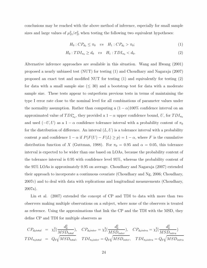
Lin et al. (2007) extended the concept of CP and TDI to data with more than two
observers making multiple observations on a subject, where none of the observers is treated
as reference. Using the approximations that link the CP and the TDI with the MSD, they
define CP and TDI for multiple observers as
CPd0total = χ21(
d20
MSDtotal), CPd0inter = χ2
1(d2
0
MSDinter), CPd0intra = χ2
1(d2
0
MSDintra)
TDIπ0total = Q0
√MSDtotal, TDIπ0inter = Q0
√MSDinter, TDIπ0intra = Q0
√MSDintra
24
where MSDtotal,MSDinter,MSDintra were defined in Section 3.2.1 under the two-way mixed
model with normality assumption. One can extend the CP and TDI to the case where the
Jth observer is treated as a reference by using the MSD for the case of the Jth observer as
a reference.
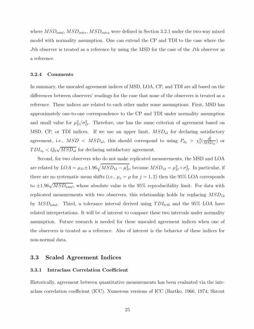
3.2.4 Comments
In summary, the unscaled agreement indices of MSD, LOA, CP, and TDI are all based on the
differences between observers’ readings for the case that none of the observers is treated as a
reference. These indices are related to each other under some assumptions. First, MSD has
approximately one-to-one correspondence to the CP and TDI under normality assumption
and small value for µ2D/σ
2D. Therefore, one has the same criterion of agreement based on
MSD, CP, or TDI indices. If we use an upper limit, MSDul for declaring satisfactory
agreement, i.e., MSD < MSDul, this should correspond to using Pd0> χ2
1(d2
0
MSDul) or
TDIπ0< Q0
√MSDul for declaring satisfactory agreement.
Second, for two observers who do not make replicated measurements, the MSD and LOA
are related by LOA = µD±1.96√MSD12 − µ2
D, because MSD12 = µ2D+σ2
D. In particular, if
there are no systematic mean shifts (i.e., µj = µ for j = 1, 2) then the 95% LOA corresponds
to ±1.96√MSDtotal, whose absolute value is the 95% reproducibility limit. For data with
replicated measurements with two observers, this relationship holds by replacing MSD12
by MSDtotal. Third, a tolerance interval derived using TDI0.95 and the 95% LOA have
related interpretations. It will be of interest to compare these two intervals under normality
assumption. Future research is needed for these unscaled agreement indices when one of
the observers is treated as a reference. Also of interest is the behavior of these indices for
non-normal data.
3.3 Scaled Agreement Indices
3.3.1 Intraclass Correlation Coefficient
Historically, agreement between quantitative measurements has been evaluated via the intr-
aclass correlation coefficient (ICC). Numerous versions of ICC (Bartko, 1966, 1974; Shrout
25

and Fleiss, 1979; Muller and Buttner, 1994; Eliasziw, et al. 1994; McGraw and Wong, 1996)
have been proposed in many areas of research by assuming different underlying ANOVA
models for the situation where none of the observers is treated as reference. In earlier re-
search on ICCs (prior to McGraw and Wong’s work in 1996), ICCs were rigorously defined as
the correlation between observations from different observers under different ANOVA model
assumptions where observers are treated as random. An ICC (denoted as ICC3c below) is
also proposed under the two-way mixed model where the observers are treated as fixed, using
the concept of correlation. The ICC3c was originally proposed by Bartko (1966) and later
corrected by Bartko (1974) and advocated by Shrout and Fleiss (1979). McGraw and Wong
(1996) suggested calling ICC3c as ICC for consistency and proposed an ICC for agreement
(denoted here as ICC3). They also added an ICC for the two-way mixed model without
interaction (denoted here as ICC2).
We unite different versions of ICCs into three ICCs under three kinds of model assumption
with unifying notations for both cases of random and fixed observers. We do not present
ICCs for averaged observations (Shout and Fleiss, 1979; McGraw and Wong, 1996), as we are
interested in agreement between single observations. We assume that each observer takes
K readings on each subject where K = 1 if there is no replication and K ≥ 2 if there
are replications (Eliasziw et al., 1994). We discuss situations of K = 1 and K ≥ 2 when
comparing ICC to CCC in Section 3.3.1. For each ICC, estimates are obtained via method of
moment based on the expectation of the mean sums of squares from these different ANOVA
models. The definitions of the three types of ICCs and their corresponding estimates are
presented below:
• ICC1 is based on a one-way random effect model without observer effect (Bartko, 1966;
Shrout and Fleiss, 1979; McGraw and Wong, 1996):
Yijk = µ+ αi + εijk
with assumptions: αi ∼ N(0, σ2α); εijk ∼ N(0, σ2
ε ); and εijk is independent of αi.
ICC1 =σ2
α
σ2α + σ2
ε
, ICC1 =MSα −MSε
MSα + (JK − 1)MSε,
where MSα and MSε are the mean sums of squares from the one-way ANOVA model
for between and within subjects, respectively.
26

• ICC2 is based on a two-way mixed or random (depending on whether the observers
are fixed or random) effect model without the observer-subject interaction (McGraw
and Wong, 1996):
Yijk = µ+ αi + βj + εijk
with assumptions: αi ∼ N(0, σ2α), εijk ∼ N(0, σ2
ε ), and εijk is independent of αi. βj
is treated as either as a fixed or a random effect, depending on whether the observers
are fixed or random. If observers are fixed, notation σ2β =
∑Jj=1 β
2j /(J − 1) is used
with constraint of∑J
j=1 βj = 0. If observers are random, additional assumptions are
βj ∼ N(0, σ2β) and αi, βj, εijk are mutually independent.
ICC2 =σ2
α
σ2α + σ2
β + σ2ε
, ICC2 =MSα −MSε
MSα + (JK − 1)MSε + J(MSβ −MSε)/n.
• ICC3 is based on a two-way mixed or random effect model (depending on whether the
observers are fixed or random) with observer-subject interaction (McGraw and Wong,
1996; Eliasziw et al., 1994).
Yijk = µ+ αi + βj + γij + εijk
with assumptions: αi ∼ N(0, σ2α), εijk ∼ N(0, σ2
ε ), and εijk is independent of αi. If
observers are fixed, notation σ2β =
∑Jj=1 β
2j /(J−1) is used with constraint of
∑Jj=1 βj =
0 and γij ∼ N(0, σ2γ). If the observers are random, additional assumptions are βj ∼
N(0, σ2β), γij ∼ N(0, σ2
γ) and αi, βj, γij, εijk are mutually independent.
ICC3(fixed βj) =σ2
α − σ2γ/(J − 1)
σ2α + σ2
β + σ2γ + σ2
e
, ICC3(random βj) =σ2
α
σ2α + σ2
β + σ2γ + σ2
e
ICC3 =MSα −MSγ
MSα + J(K − 1)MSε + (J − 1)MSγ + J(MSβ −MSγ)/n.
As mentioned earlier, Bartko (1974) and Shrout and Fleiss (1979) presented the following
ICC, later called ICC for consistency (e.g., observers are allowed to differ by a fixed constant)
by McGraw and Wang (1996) using
ICC3c =σ2
α − σ2γ/(J − 1)
σ2α + σ2
γ + σ2ε
27
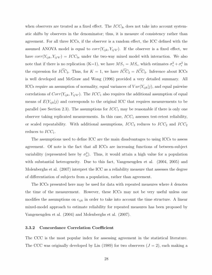
when observers are treated as a fixed effect. The ICC3c does not take into account system-
atic shifts by observers in the denominator; thus, it is measure of consistency rather than
agreement. For all three ICCs, if the observer is a random effect, the ICC defined with the
assumed ANOVA model is equal to corr(Yijk, Yij′k′). If the observer is a fixed effect, we
have corr(Yijk, Yij′k′) = ICC3c under the two-way mixed model with interaction. We also
note that if there is no replication (K=1), we have MSγ = MSε, which estimates σ2γ + σ2
ε in
the expression for ICC3. Thus, for K = 1, we have ICC2 = ICC3. Inference about ICCs
is well developed and McGraw and Wong (1996) provided a very detailed summary. All
ICCs require an assumption of normality, equal variances of V ar(Yijk|j), and equal pairwise
correlations of Corr(Yijk, Yij′k′). The ICC1 also requires the additional assumption of equal
means of E(Yijk|j) and corresponds to the original ICC that requires measurements to be
parallel (see Section 2.3). The assumptions for ICC1 may be reasonable if there is only one
observer taking replicated measurements. In this case, ICC1 assesses test-retest reliability,
or scaled repeatability. With additional assumptions, ICC3 reduces to ICC2 and ICC2
reduces to ICC1.
The assumptions used to define ICC are the main disadvantages to using ICCs to assess
agreement. Of note is the fact that all ICCs are increasing functions of between-subject
variability (represented here by σ2α). Thus, it would attain a high value for a population
with substantial heterogeneity. Due to this fact, Vangeneugden et al. (2004, 2005) and
Molenberghs et al. (2007) interpret the ICC as a reliability measure that assesses the degree
of differentiation of subjects from a population, rather than agreement.
The ICCs presented here may be used for data with repeated measures where k denotes
the time of the measurement. However, these ICCs may not be very useful unless one
modifies the assumptions on εijk in order to take into account the time structure. A linear
mixed-model approach to estimate reliability for repeated measures has been proposed by
Vangeneugden et al. (2004) and Molenberghs et al. (2007).
3.3.2 Concordance Correlation Coefficient
The CCC is the most popular index for assessing agreement in the statistical literature.
The CCC was originally developed by Lin (1989) for two observers (J = 2), each making a
28

single reading on a subject. It was later extended to multiple J observers for data without
replications (Lin, 1989; King and Chinchilli, 2001a; Lin, et al. 2002, Barnhart et al., 2002)
and for data with replications (Barnhart et al., 2005a, Lin et al., 2007) where none of the
observers is treated as reference. These extensions included the original CCC for J = 2
as a special case. Recently, Barnhart et al. (2007b) extended the CCC to the situation
where one of the multiple observers is treated as reference. Barnhart and Williamson (2001)
used a generalized estimating equations (GEE) approach to modeling pairwise CCCs as a
function of covariates. Chinchilli et al. (1996) and King et al. (2007a, 2007b) extended the
CCC for data with repeated measures comparing two observers. Quiroz (2005) extends the
CCC for data with repeated measures comparing multiple observers by using the two-way
ANOVA model without interaction. Due to the assumptions of the ANOVA model, the CCC
defined by Quiroz (2005) is the special case of CCC by Barnhart et al. (2005a) for data with
replications.
We first present the total CCC, inter-CCC, and intra-CCC for multiple observers for data
with replications where none of the observers is treated as a reference. Of note here is the
fact that the total CCC is the usual CCC for data without replications. The definition of
the total CCC does not require replicated data (King and Chinchilli, 2001a, Barnhart et al,
2002), although one can estimate both the between-subject (σ2Bj) and within-subject (σ2
Wj)
variabilities for data with replications, while only total variability (σ2j = σ2
Bj + σ2Wj) can be
estimated for data without replications. One cannot estimate inter- or intra-CCCs for data
without replications.
Let Yijk be the kth replicated measurements for the ith subject by the jth method and
write Yijk = µij + εijk with the assumptions and notations in the begining of Section 3. The
CCC for assessing agreement between J observers using data with or without replications
can be written
CCCtotal = ρc = 1 −∑J−1
j=1
∑Jj′=j+1E(Yijk − Yij′k′)2
∑J−1j=1
∑Jj′=j+1EI(Yijk − Yij′k′)2
(3)
=2
∑J−1j=1
∑Jj′=j+1 σjσj′ρjj′
(J − 1)∑J
j=1 σ2j +
∑J−1j=1
∑Jj′=j+1(µj − µj′)2
(4)
=2
∑J−1j=1
∑Jj′=j+1 σBjσBj′ρµjj′
∑J−1j=1
∑Jj′=j+1[2σBjσBj′ + (µj − µj′)2 + (σBj − σBj′)2 + σ2
Wj + σ2Wj′]
,(5)
29
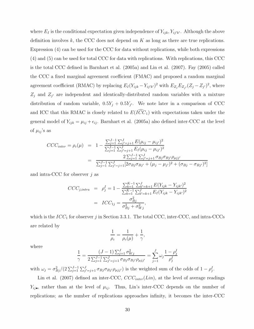
where EI is the conditional expectation given independence of Yijk, Yij′k′ . Although the above
definition involves k, the CCC does not depend on K as long as there are true replications.
Expression (4) can be used for the CCC for data without replications, while both expressions
(4) and (5) can be used for total CCC for data with replications. With replications, this CCC
is the total CCC defined in Barnhart et al. (2005a) and Lin et al. (2007). Fay (2005) called
the CCC a fixed marginal agreement coefficient (FMAC) and proposed a random marginal
agreement coefficient (RMAC) by replacing EI(Yijk −Yij′k′)2 with EZjEZj′
(Zj −Zj′)2, where
Zj and Zj′ are independent and identically-distributed random variables with a mixture
distribution of random variable, 0.5Yj + 0.5Yj′. We note later in a comparison of CCC
and ICC that this RMAC is closely related to E( ICC1) with expectations taken under the
general model of Yijk = µij + εij . Barnhart et al. (2005a) also defined inter-CCC at the level
of µij’s as
CCCinter = ρc(µ) = 1 −∑J−1
j=1
∑Jj′=j+1E(µij − µij′)
2
∑J−1j=1
∑Jj′=j+1EI(µij − µij′)2
=2
∑J−1j=1
∑Jj′=j+1 σBjσBj′ρµjj′
∑J−1j=1
∑Jj′=j+1[2σBjσBj′ + (µj − µj′)2 + (σBj − σBj′)2]
and intra-CCC for observer j as
CCCj,intra = ρIj = 1 −
∑K−1k=1
∑Jk′=k+1E(Yijk − Yijk′)2
∑K−1k=1
∑Jk′=k+1EI(Yijk − Yijk′)2
= ICC1j =σ2
Bj
σ2Bj + σ2
Wj
,
which is the ICC1 for observer j in Section 3.3.1. The total CCC, inter-CCC, and intra-CCCs
are related by1
ρc
=1
ρc(µ)+
1
γ,
where1
γ=
(J − 1)∑J
j=1 σ2Wj
2∑J−1
j=1
∑Jj′=j+1 σBjσBj′ρµjj′
=J∑
j=1
ωj
1 − ρIj
ρIj
with ωj = σ2Bj/(2
∑J−1j=1
∑Jj′=j+1 σBjσBj′ρµjj′) is the weighted sum of the odds of 1 − ρI
j .
Lin et al. (2007) defined an inter-CCC, CCCinter(Lin), at the level of average readings
Yij•, rather than at the level of µij. Thus, Lin’s inter-CCC depends on the number of
replications; as the number of replications approaches infinity, it becomes the inter-CCC
30
defined by Barnhart et al. (2005a), (i.e., CCCinter(Lin) → CCCinter as K → ∞). Lin et al.
(2007) also define an overall intra-CCC, rather than separate intra-CCCs for each observer.
This overall intra-CCC is the average of the J intra-CCCs above.
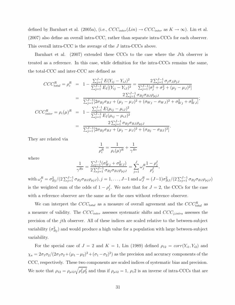
Barnhart et al. (2007) extended these CCCs to the case where the Jth observer is
treated as a reference. In this case, while definition for the intra-CCCs remains the same,
the total-CCC and inter-CCC are defined as
CCCRtotal = ρR
c = 1 −∑J−1
j=1 E(Yij − YiJ)2
∑J−1j=1 EI [(Yij − YiJ)2
=2
∑J−1j=1 σjσJρjJ
∑J−1j=1 [σ2
j + σ2J + (µj − µJ)2]
=2
∑J−1j=1 σBjσBJρµjJ
∑J−1j=1 [2σBjσBJ + (µj − µJ)2 + (σWj − σWJ)2 + σ2
Wj + σ2WJ ]
;
CCCRinter = ρc(µ)R = 1 −
∑J−1j=1 E(µij − µiJ)2
∑J−1j=1 EI(µij − µiJ)2
=2
∑J−1j=1 σBjσBJρµjJ
∑J−1j=1 [2σBjσBJ + (µj − µJ)2 + (σBj − σBJ )2]
.
They are related via1
ρRc
=1
ρc(µ)R+
1
γR∗
where1
γR∗=
∑J−1j=1 (σ2
Wj + σ2WJ)
2∑J−1
j=1 σBjσBJρµjJ
=J∑
j=1
ωRj
1 − ρIj
ρIj
,
with ωRj = σ2
Bj/(2∑J−1
j=1 σBjσBJρµjJ), j = 1, . . . , J−1 and ωRJ = (J−1)σ2
BJ/(2∑J−1
j=1 σBjσBJρµjJ)
is the weighted sum of the odds of 1 − ρIj . We note that for J = 2, the CCCs for the case
with a reference observer are the same as for the ones without reference observer.
We can interpret the CCCtotal as a measure of overall agreement and the CCCRtotal as
a measure of validity. The CCCinter assesses systematic shifts and CCCj,intra assesses the
precision of the jth observer. All of these indices are scaled relative to the between-subject
variability (σ2Bj) and would produce a high value for a population with large between-subject
variability.
For the special case of J = 2 and K = 1, Lin (1989) defined ρ12 = corr(Yi1, Yi2) and
χa = 2σ1σ2/(2σ1σ2 +(µ1−µ2)2+(σ1−σ2)
2) as the precision and accuracy components of the
CCC, respectively. These two components are scaled indices of systematic bias and precision.
We note that ρ12 = ρµ12
√ρI
1ρI2 and thus if ρµ12 = 1, ρ12 is an inverse of intra-CCCs that are
31

scaled indices of within-subject variabilities σ2Wj. We note that χa assesses the systematic
bias due to both location and scale shifts.
If the agreement between multiple observers is not satisfactory based on the CCCs, it
is useful to compare the pairwise CCCs of multiple observers to find which observers do
not agree well. One may be also interested in whether there is a trend in the agreement,
or whether the observers have good or poor agreement in particular subgroups. Barnhart
and Williamson (2001) used the GEE approach to compare these pairwise CCCs and to
investigate the impact of covariates. One should be cautious in interpreting CCCs when
covariates are used in modeling. Because CCCs depend on between-subject variability, one
must ensure that between-subject variability is similar across the range of covariate values.
CCC values may decrease due to decreased between-subject variability when considering
subgroups of different covariate values. The GEE approach can be extended to compare
CCCs over time in cases where time is a covariate. Specifically, for data with repeated
measures, and using J = 2 as an example, CCCs can be computed at each time point, and
one can model CCCs with Fisher’s Z-transformation as a function of time. If there is no
time effect, one can obtain a common CCC that is aggregated over time. This common CCC
is similar to the straight average of CCCs computed from each time point, but differs from
the CCC discussed below by Chinchilli et al. (1996) and King et al. (2007a) for repeated
measures.
For two observers (J=2), Chinchilli et al. (1996) proposed weighted CCC, CCC(w), and
King et al. (2007a) proposed repeated measures CCC, CCC(rm), for data with repeated
measures. The repeated measurements can occur due to multiple visits in longitudinal
studies, or arise when multiple subsamples are split from from the original sample. The
repeated measures are not considered replications because they may not be independently
and identically distributed, given subject or sample. Suppose that for each observer, there
are p repeated measures for a subject, rather than K replications. There are then a total of
p2 pairs of measurements between the two observers, one from method Y1 and the other from
method Y2. Intuitively, one can assess agreement by using an agreement matrix CCCp×p
consisting of all pairwise CCCs based on the p2 pairs of measurements using Lin’s (1989)
original definition of CCC. These pairwise CCCs are concerned with agreement between
32
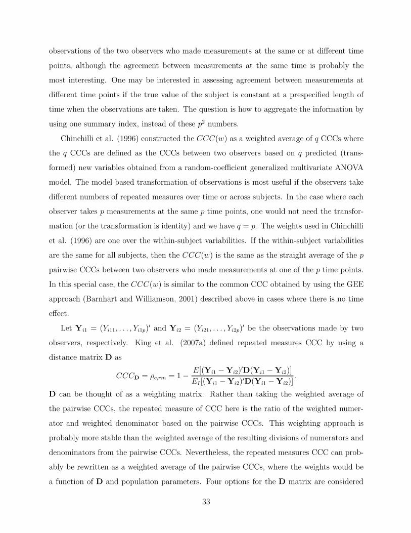
observations of the two observers who made measurements at the same or at different time
points, although the agreement between measurements at the same time is probably the
most interesting. One may be interested in assessing agreement between measurements at
different time points if the true value of the subject is constant at a prespecified length of
time when the observations are taken. The question is how to aggregate the information by
using one summary index, instead of these p2 numbers.
Chinchilli et al. (1996) constructed the CCC(w) as a weighted average of q CCCs where
the q CCCs are defined as the CCCs between two observers based on q predicted (trans-
formed) new variables obtained from a random-coefficient generalized multivariate ANOVA
model. The model-based transformation of observations is most useful if the observers take
different numbers of repeated measures over time or across subjects. In the case where each
observer takes p measurements at the same p time points, one would not need the transfor-
mation (or the transformation is identity) and we have q = p. The weights used in Chinchilli
et al. (1996) are one over the within-subject variabilities. If the within-subject variabilities
are the same for all subjects, then the CCC(w) is the same as the straight average of the p
pairwise CCCs between two observers who made measurements at one of the p time points.
In this special case, the CCC(w) is similar to the common CCC obtained by using the GEE
approach (Barnhart and Williamson, 2001) described above in cases where there is no time
effect.
Let Yi1 = (Yi11, . . . , Yi1p)′ and Yi2 = (Yi21, . . . , Yi2p)
′ be the observations made by two
observers, respectively. King et al. (2007a) defined repeated measures CCC by using a
distance matrix D as
CCCD = ρc,rm = 1 − E[(Yi1 − Yi2)′D(Yi1 − Yi2)]
EI [(Yi1 − Yi2)′D(Yi1 − Yi2)].
D can be thought of as a weighting matrix. Rather than taking the weighted average of
the pairwise CCCs, the repeated measure of CCC here is the ratio of the weighted numer-
ator and weighted denominator based on the pairwise CCCs. This weighting approach is
probably more stable than the weighted average of the resulting divisions of numerators and
denominators from the pairwise CCCs. Nevertheless, the repeated measures CCC can prob-
ably be rewritten as a weighted average of the pairwise CCCs, where the weights would be
a function of D and population parameters. Four options for the D matrix are considered
33
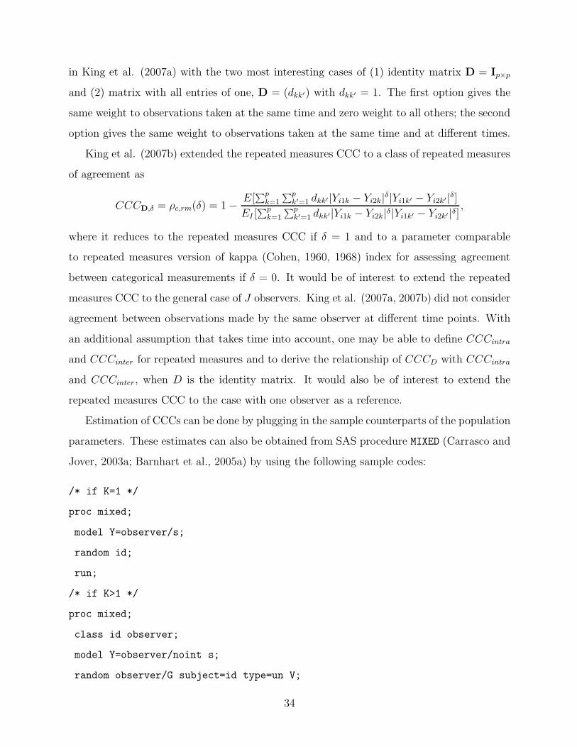
in King et al. (2007a) with the two most interesting cases of (1) identity matrix D = Ip×p
and (2) matrix with all entries of one, D = (dkk′) with dkk′ = 1. The first option gives the
same weight to observations taken at the same time and zero weight to all others; the second
option gives the same weight to observations taken at the same time and at different times.
King et al. (2007b) extended the repeated measures CCC to a class of repeated measures
of agreement as
CCCD,δ = ρc,rm(δ) = 1 − E[∑p
k=1
∑pk′=1 dkk′|Yi1k − Yi2k|δ|Yi1k′ − Yi2k′|δ]
EI [∑p
k=1
∑pk′=1 dkk′|Yi1k − Yi2k|δ|Yi1k′ − Yi2k′|δ] ,
where it reduces to the repeated measures CCC if δ = 1 and to a parameter comparable
to repeated measures version of kappa (Cohen, 1960, 1968) index for assessing agreement
between categorical measurements if δ = 0. It would be of interest to extend the repeated
measures CCC to the general case of J observers. King et al. (2007a, 2007b) did not consider
agreement between observations made by the same observer at different time points. With
an additional assumption that takes time into account, one may be able to define CCCintra
and CCCinter for repeated measures and to derive the relationship of CCCD with CCCintra
and CCCinter, when D is the identity matrix. It would also be of interest to extend the
repeated measures CCC to the case with one observer as a reference.
Estimation of CCCs can be done by plugging in the sample counterparts of the population
parameters. These estimates can also be obtained from SAS procedure MIXED (Carrasco and
Jover, 2003a; Barnhart et al., 2005a) by using the following sample codes:
/* if K=1 */
proc mixed;
model Y=observer/s;
random id;
run;
/* if K>1 */
proc mixed;
class id observer;
model Y=observer/noint s;
random observer/G subject=id type=un V;
34

repeated /R group=observer;
run;
where the solution in the model statement provides the estimates for µj’s, the G matrix
provides the estimates for σ2Bj and ρµjj′, and the R matrix provides the estimates for σ2
Wj.
Carrasco and Jover (2003a) noted that (Y•j• − Y•j′•)2 is a biased estimator of (µj − µj′)
2
because E(Y•j• − Y•j′•)2 = (µj − µj′)
2 + V ar(Y•j•) + V ar(Y•j′•) − 2Cov(Y•j•, Y•j′•) = (µj −µj′)
2+σ2Bj/n+σ2
Wj/(nK)+σ2Bj′/n+σ2
Wj′/(nK)−2σBjσBj′ρµjj′/n. The bias may be negligible
for moderate-to-large sample sizes.
Parametric, semiparametric, and nonparametric approaches have been proposed for infer-
ence of CCCs. If we assume normality of the data, asymptotic distribution of the estimated
CCCs may be used for inference (Lin, 1989; Carrasco and Jover, 2003a). The semipara-
metric approach is available via GEE approach (Barnhart and Williamson, 2001; Lin et al.,
2007) and the nonparametric approach was proposed by King and Chinchilli (2001a) using
U-statistics. Williamson et al. (2007) proposed and compared permutation and bootstrap
tests for testing equalities of CCCs under various conditions. The permutation test is only
valid if the joint distributions of the observations under these various conditions are the
same, an assumption that may be difficult to verify. Thus, bootstrap-based test may be
preferred.
Comparison of CCC and ICC
While (total) CCC and ICC are similar indices, there are some differences between them:
(1) the ICC has been proposed for both fixed and random observers, while the CCC usually
treats the observers fixed; and (2) the ICC requires ANOVA model assumptions, while
the CCC does not. However, in specific cases, the ICC and CCC are the same or have
similar values (Nickerson, 1997; Carrasco and Jover, 2003a). For example, if there are no
replications, Carrasco and Jover (2003a) demonstrated that ICC2 is the same as total CCC
even without the ANOVA model assumption. In general, if the ANOVA model assumptions
are correct, the CCC under this model reduces to the ICC defined by this ANOVA model.
ICC estimators are based on unbiased estimates for the parameters used in the assumed
ANOVA models. However, it is not clear what the ICC estimators are estimating if the
assumed ANOVA models are not correct. Using a general model of Yijk = µij + εijk, Chen
35

and Barnhart (2007) compared expected values of the three ICC estimators in Section 3.3.1
under this general model to the total CCC under the same model. They approximated
the expected values of the ICC estimators by taking the expectation of the numerator and
denominator under this general model. They found that if there are no replications (K=1),
E( ICC1) may be smaller or larger than the CCC, where for J = 2,
E( ICC1) =2ρσ1σ2 − 0.5(µ1 − µ2)
2
σ21 + σ2
2 + 0.5(µ1 − µ2)2.
We note that this E( ICC1) is the same as the random marginal agreement coefficient
(RMAC) proposed by Fay (2005) for continuous response. For ICC2 and ICC3, we have
equality, i.e, E( ICC2) = E( ICC3) = CCC. For data with replications (K > 1), Chen
and Barnhart (2007) found that under the general model, E( ICC3) = CCC. However, the
expected ICCs for the first two ICC estimators depend on the number of replications, K,
whereas the CCC does not depend on K. For the special case with homogeneous between-
and within-subject variability; i.e., σ2Bj = σ2
B, σ2Wj = σ2
W , both E( ICC1) and E( ICC2) are
increasing functions of K. E( ICC1) starts with a value that may be less or greater than
the CCC at K = 1 and increases quickly to the limit (as K → ∞) that exceeds the CCC.
E( ICC2) equals the CCC at K = 1 and increases quickly to the limit (as K → ∞) that also
exceeds the CCC.
Note that even in the case of E( ICC) = CCC under the general model, we may still
have ICC ≤ ICC, because the plug-in estimator of CCC, ICC, is biased due to a biased
estimation of (µj − µj′)2 via (Y•j• − Y•j′•)
2 (Carrasco and Jover, 2003a; Nickerson, 1997).
We have ICC = ICC only if a bias correction term is used for estimating (µj − µj′)2 in the
CCC.
3.3.3 Coefficient of Individual Agreement
The CCC is known to depend on between-subject variability that may result from that fact
that it is scaled relative to the maximum disagreement defined as the expected squared differ-
ence under independence. Barnhart and colleagues (Haber and Barnhart, 2007; Barnhart et
al., 2007a) began looking for a scaled agreement index, the coefficient of individual agreement
(CIA), which is scaled relative to the minimum or acceptable disagreement, with the goal
36

of establishing interchangeability of observers. Before considering observers for comparison,
one must assume that the replication errors of the observers are acceptable. This is espe-
cially true for the reference observer. Thus, they used the disagreement between replicated
measurements within an observer as a yardstick for acceptable disagreement. Intuitively,
interchangeability is established only if individual measurements from different observers are
similar to replicated measurements of the same observer. In other words, the individual
difference between measurements from different observers is relatively small, so that this
difference is close to the difference of replicated measurements within an observer. This
concept of individual agreement is closely linked to the concept of individual bioequivalence
in bioequivalence studies (Anderson and Hauk, 1990; Schall and Luus, 1993).
Replicated measurements by observers are needed for the CIAs for the purpose of estima-
tion and inference only. Regardless of the number of replications, CIAs assesses agreement
between observers when each observer evaluates each subject only once. The coefficients are
intended to be used to decide whether a single measurement made by one observer can be
replaced by a single measurement made by another observer in practice, when each subject
is evaluated only once by each observer. Let Yijk = µij + εijk with the assumptions in section
3.1. Barnhart et al. (2007a) defined the CIAs for cases of no reference observer and the Jth
observer as a reference with
CIAN = ψN =
∑Jj=1E(Yijk − Yijk′)2/2
∑J−1j=1
∑Jj′=j+1E[(Yijk − Yij′k′)2]/(J − 1)
(where k 6= k′)
=
∑J−1j=1
∑Jj′=j+1(σ
2Wj + σ2
Wj′)∑J−1j=1
∑Jj′=j+1[2(1 − ρµjj′)σBjσBj′ + (µj − µj′)2 + (σBj − σBj′)2 + σ2
Wj + σ2Wj′]
,
CIAR = ψR =E(YiJk − YiJk′)2/2
∑J−1j=1 E[(Yijk − YiJk′)2]/(J − 1)
(where k 6= k′)
=σ2
WJ∑J−1j=1 [2(1 − ρµjJ)σBjσBJ + (µj − µJ)2 + (σBj − σBJ )2 + σ2
Wj + σ2WJ ]
.
respectively. These are the CIAs when the MSD function is used as a disagreement function.
For J = 2, Haber and Barnhart (2007) extended the CIAs to the general disagreement
function and illustrated the methodology with various disagreement functions. Barnhart et
al. (2007a) showed that there are one-to-one relationships between the CIAN and the two
previously proposed agreement indices by Haber et al. (2005) and Shao and Zhong (2004).
Estimates of CIAs can be obtained by the method of moment and can be computed
37
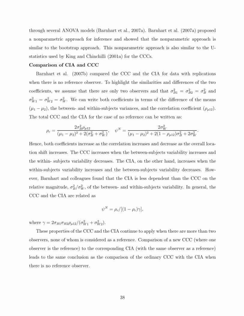
through several ANOVA models (Barnhart et al., 2007a). Barnhart et al. (2007a) proposed
a nonparametric approach for inference and showed that the nonparametric approach is
similar to the bootstrap approach. This nonparametric approach is also similar to the U-
statistics used by King and Chinchilli (2001a) for the CCCs.
Comparison of CIA and CCC
Barnhart et al. (2007b) compared the CCC and the CIA for data with replications
when there is no reference observer. To highlight the similarities and differences of the two
coefficients, we assume that there are only two observers and that σ2B1 = σ2
B2 = σ2B and
σ2W1 = σ2
W2 = σ2W . We can write both coefficients in terms of the difference of the means
(µ1 − µ2), the between- and within-subjects variances, and the correlation coefficient (ρµ12).
The total CCC and the CIA for the case of no reference can be written as:
ρc =2σ2
Bρµ12
(µ1 − µ2)2 + 2(σ2B + σ2
W ), ψN =
2σ2W
(µ1 − µ2)2 + 2(1 − ρµ12)σ2B + 2σ2
W
.
Hence, both coefficients increase as the correlation increases and decrease as the overall loca-
tion shift increases. The CCC increases when the between-subjects variability increases and
the within- subjects variability decreases. The CIA, on the other hand, increases when the
within-subjects variability increases and the between-subjects variability decreases. How-
ever, Barnhart and colleagues found that the CIA is less dependent than the CCC on the
relative magnitude, σ2B/σ
2W , of the between- and within-subjects variability. In general, the
CCC and the CIA are related as
ψN = ρc/[(1 − ρc)γ],
where γ = 2σB1σB2ρµ12/(σ2W1 + σ2
W2).
These properties of the CCC and the CIA continue to apply when there are more than two
observers, none of whom is considered as a reference. Comparison of a new CCC (where one
observer is the reference) to the corresponding CIA (with the same observer as a reference)
leads to the same conclusion as the comparison of the ordinary CCC with the CIA when
there is no reference observer.
38

3.3.4 Dependability Coefficient and Generalizability Coefficient
Generalizability theory (GT) extends the concept of reliability based on classical theory
(CT) to account for various sources of variability and different kinds of decisions. We first
introduce the CT that defines the traditional reliability coefficient, followed by a single-facet
design and a multi-facet design in GT, where we discuss the definition of dependability
coefficient and generalizability coefficient.
In CT, an observation is decomposed as the sum of the subject’s true score, plus the
random measurement error. In the simple case that an observation is made by an observer,
let Yij be the observations made by the jth observer on subject i. Then, the one-way ANOVA
model Yij = µi + εij = µ + αi + εij is used in CT, where observations Yij are assumed to
be parallel (see Section 2.3 under reliability). The reliability is defined as ICC1 (see section
3.3.1) and can be viewed either as the ratio of the true score variance (V ar(µi) = σ2α) over
the observed variance (V ar(Yij) = σ2α + σ2
ε ) or as correlation Corr(Yij, Yij′).
In GT, the assumption of parallel observations is relaxed by decomposing an observation
as sum of subject’s universe score and the multiple sources of components that contribute
to the variability of the observed value, where the universe score is similar to the concept of
true score in CT. The subject is usually called the facet of differentiation or the object (facet)
of measurement and the components are called facets of generalization. The levels of facets
of generalization are called conditions. The universe is defined as all observations made
under all conditions of the facets of generalization. The universe score is the average of all
possible (usually infinite) observations in the universe, similar to the true score in CT. The
simplest case is the single facet design, where the observer is the only facet of generalization.
The universe is all observations made by all (possibly infinite) observers, and the universe
score is the average of these observations. GT consists of generalization studies (G-studies)
and decision studies (D-studies), where G-studies investigate the variance components due
to facets of differentiation and facets of generalization, while D-studies investigate various
designs based on particular decisions. In general, one G-study is planned to include all
possible facets of generalization (i.e., sources of possible variabilities), while multiple D-
studies can be formulated by considering the variance components obtained from a single
G-study in various ways.
39

One key convention in GT is that all facets of generalization are considered as random
effects. Thus, the observer is treated as random and the GT extends the reliability concept
in Section 3.3.1 for the case of the random observer only. Fixed facets of generalization are
discussed in Molenberghs et al. (2007).
Let Yijk be the kth replication (k = 1, . . . , K) made by observer j on subject i. Usually,
K = 1 in the GT, but we allow general K for comparison with the reliability concept
in Section 3.3.1 that includes both K = 1 and K > 1. In a single-facet study, the G-
study may consider the following three random effect models: (1) Yijk = µ + αi + εijk; (2)
Yijk = µ + αi + βj + εijk; and (3) Yijk = µ + αi + βj + (αβ)ij + εijk, where µi = µ + αi is
the universe score. Model (1) is usually not considered in a G-study because the observer is
recognized as a facet and thus should always be considered as a factor in the ANOVA model.
In general, the G-study uses model (2) if there are no replications and model (3) if there
are replications. We include all three models for comparison with the ICCs. The G-study
uses these ANOVA models to estimate and perform inference on variance components of
V ar(µi) = σ2α, V ar(βj) = σ2
β, V ar(αβij) = σ2αβ , V ar(εij) = σ2
ε due to facet of differentiation
(subject) and facets of generalization (observer and replication), respectively.
In D-studies, one must decide (1) whether the decision is absolute or relative and (2)
whether a single observation, or average of several observations of a subject, is used in prac-
tice. An absolute decision is concerned with obtaining the estimate of a subject’s universe
score regardless of another subject’s universe score while relative decision is concerned with
rank-ordering subjects. Thus, the absolute decision is relevant to absolute agreement con-
sidered in this paper, while the relative decision is relevant to consistency agreement, such as
ICC, for consistency. As mentioned in the begining of Section 3.1, we only consider the case
that a single observation will be used in practice. Therefore, we focus our attention on the
D-study with absolute decision, with the purpose of using a single observation in practice.
Coefficients that depend on relative decision with the purpose of using a single observation
in practice are mentioned here for contrast. Based on the absolute decision, dependability
coefficient (DC) is defined as
ρDC =variance of universe score based on facet of differentiation
variance of universe score + variance of absolute error.
40

Based on the relative decision, generalizability coefficient (GC) is defined as
ρGC =variance of universe score based on facet of differentiation
variance of universe score + relative error.
In the single-facet design, the universe score for subject i is µi = µ + αi, and the absolute
error (∆ijk) is the difference between the observed score and the universe score, ∆ijk =
Yijk − µi. The relative error (δijk) is defined as the difference of the subject’s observed
deviation score (Yijk −E(Yijk|j, k) = Yijk −µ−βj) and the universe deviation score (µi−µ),
δijk = Yijk−µi−βj . Intuitively, the relative error does not contain the observer effect, because
this effect does not affect the subject’s ranking. Table 1 shows the dependability coefficient
and generalizability coefficient based on the three different ANOVA models. It can be shown
that ρDC = corr(Yijk, Yij′k′) and ρGC = corr(Yijk, Yij′k′|j, j′, k, k′), where j 6= j′, k 6= k′ for
all three models (Molenberghs et al., 2007). Thus, the DC can be interpreted as correlation
and the GC can be interpreted as conditional correlation.
Table1. Dependability and Generalizability Coefficients for one-facet design
G-study Models D-study coefficients
ρDC ρGC relation with ICC
(1) Yijk = µ+ αi + εijkσ2
α
σ2α+σ2
ε
σ2α
σ2α+σ2
ερDC = ρGC = ICC1
(2) Yijk = µ+ αi + βj + εijkσ2
α
σ2α+σ2
β+σ2
ε
σ2α
σ2α+σ2
ερDC = ICC2, ρGC = ICC1
(3) Yijk = µ+ αi + βj + αβij + εijkσ2
α
σ2α+σ2
β+σ2
αβ+σ2
ε
σ2α
σ2α+σ2
αβ+σ2
ερDC = ICC3, ρGC = ICC3c
Molenberghs et al. (2007) also considered the single-facet design with a fixed observer
and the facet of generalization as the replication. One may consider separate ANOVA models
to obtain DC and GC for each observer; however, if model (3) is used, the DC and GC for
each observer is the same and equal to
ρtest−retest = corr(Yijk, Yijk′|j) = corr(Yijk, Yijk′|j, k, k′) =σ2
α + σ2(αβ)
σ2α + σ2
(αβ) + σ2ε
that is considered as test-retest reliability, which is the same as the intra-CCC by Lin et al.
(2007).
It is now easy to extend the single-facet design to the multifacet design. For illustration,
let Yijtc denote the observation made by observer j at time t on subject i, with covariate value
41

c. The facets of generalization are observer, time, and covariate. The G-study decomposes
Yijtc as the sum of various sources of variability with model (4) below:
(4) Yijtc = µ+ αi + βj + τt + θc + (αβ)ij + (ατ)it + (αθ)ic +
(βτ)jt + (βθ)jc + (τθ)tc + (αβτ)ijt + (αβθ)ijc + (ατθ)itc + (βτθ)jtc + εijtc
The DC and GC from the D-studies with absolute and relative errors are
ρDC =σ2
α
σ2α + σ2
β + σ2τ + σ2
θ + σ2(αβ) + σ2
(βθ) + σ2(τθ) + σ(ατθ)2 + σ2
(βτθ) + σ2ε
ρGC =σ2
α
σ2α + σ2
(αβ) + σ2(ατθ) + σ2
ε
,
respectively. One should note that these coefficients now assess interchangeability for the
measurements by different observers at different time points and different covariate condi-
tions, not only for interchangeability of the observers.
Other DCs or GCs may be formed if we consider different facets of differentiation other
than subject; e.g., subject-by-country, or subject-by-observer. Vaneneugden et al. (2005)
and Molenberghs et al. (2007) extended the concepts of ICC and GT to longitudinal data
in the framework of a linear mixed-effect model with and without serial correlation. The
mixed effect model allows for adjustment of fixed effects from covariates such as treatment.
In their framework, both the ICC and DC are expressed as correlations, while the GC is
expressed as a conditional correlation. In the simple case where Yijt is the observation made
by observer j on subject i at time t, the mixed model is Yijt = µ+αi +βj +(αβ)ij +ωit + εijt,
where ωit accounts for serial correlation. They first defined ICC as ICC = corr(Yijt, Yijt′)
for test-retest reliability and then defined three DCs and three GCs for overall, test-retest,
and interrater respectively as
ρDC = corr(Yijt, Yij′t′), ρGC = corr(Yijt, Yij′t′ |j, j′, t, t′)
ρDC,test−retest = corr(Yijt, Yijt′), ρGC,test−retest = corr(Yijt, Yijt′|jt, t′)
ρDC,inter−rater = corr(Yijt, Yij′t), ρGC,inter−rater = corr(Yijt, Yij′t|j, j′, t).
If the repeated measurements are treated as replicated measurements by setting ωit = 0 in
the model, then ρDC = ρDC,inter−rater. Furthermore, ρDC and ρDC,test−retest correspond to
42
the total CCC and intra-CCC, respectively, if we set σ2β =
∑Jj=1(µj −µ•)
2/(J − 1). For data
with repeated measures, ρDC,inter−rater has an interpretation similar to the CCCD by King et
al. (2007a) with corresponding D matrix. We should point out that the models used in GT
assume the same between-subject variability, while the CCC allows separate between-subject
variability for each observer.
In summary, GT provides a flexible way to investigate interchangeability of levels in more
than one factor (such as observer). However, the DC shares the same property as the ICC
and CCC, in that its value increases as the variability of between-subject increases. Thus,
one cannot compare the coefficients formed from different G-studies where the populations
differ greatly.
3.3.5 Comments
In summary, the scaled agreement indices of ICC, CCC, CIA and DC are all standardized to
have values between -1 and 1. The ICC, CCC, and DC are related and depend on between-
subject variability and may produce high values for heterogeneous populations (Atkinson
and Nevill, 1997; Bland and Altman, 1990). The ICC can accomodate multiple fixed and
random observers, but is not suited for cases with a reference observer or for data with
repeated measures, without additional assumptions. The CCC is mainly developed for fixed
observers and reduces to the ICC for fixed observers under additional assumptions. The
CCC formulation may be used for the case with random observers, but additional care is
needed for inference. The DC is an extension of the ICC for random observers that can be
used for situations with multiple factors, and for data with repeated measurements. There
has been limited development of the DC for fixed observers; nothing has been developed
for the case with a reference observer. The CIA is fundamentally different from the ICC,
CCC, and DC because it uses within-subject, rather than between-subject, variability as the
scaling factor. It is possible to have high ICC/CCC/DC value and low CIA value (and vice
versa) from the same data set. See Barnhart et al. (2007b) for additional details.
43

4 Discussion
We have reviewed the concepts and statistical approaches for assessing agreement with con-
tinuous measurements based on classification of (1) descriptive tools, (2) unscaled indices,
and (3) scaled indices. An alternative classification used in individual bioequivalence litera-
ture (Chen, 1997) also may be considered: (1) aggregated criteria, (2) disaggregated criteria,
and (3) probability criteria . The classification of aggregated criteria is based on an index
that combines different sources of possible disagreement among observers. Sources of dis-
agreement may arise from differing population means, differing between-subject variances,
differing within-subject variances among observers, poor correlation between measurements
made by observers, and large subject-by- observer interaction. Disaggregated criteria exam-
ine these various possible sources of disagreement separately (see Lee, et al., 1989). Except
for the CP and TDI, which are based on probability criteria, all other indices reviewed here
are aggregated indices. Our descriptive tools are intuitive approaches to disaggregated cri-
teria. As pointed out by Chen (1997), aggregated criteria have the advantage of balancing
different sources of disagreement while disaggregated criteria may have the advantage of
identifying the actual source of disagreement if the agreement is not satisfactory. However,
disaggregated criteria may encounter the problem of multiple testing if the criteria do not
use one procedure to test multiple hypotheses together. We did not review disaggregated
criteria for assessing agreement that takes into account multiple testing; readers are instead
directed to the literature that were based on the intersection-union principle (Carrasco and
Jover, 2003b, 2005a; Choudhary and Nagaraja, 2005a) or other single procedures (Bartko,
1994)..
We summarize here the unscaled (Table 2) and scaled (Table 3) agreement indices ac-
cording to whether there is an existing method for different types of data structure. The
tables indicate that future research is needed for agreement indices where there are repeated
measures, covariates, and the existence of a reference observer. Furthermore, most method-
ologies were developed for fixed observers; thus, further research is needed for the case of
random observers. The case of random observers should be considered if different observers
from a pool of observers, rather than the same limited observers, are used in practice or in
44

research. Recently, Barnhart et al. (2005b) used the CCC index and Choudhary (2007) used
the CP and TDI indices to assess agreement of measurements subject to censoring due to the
limit of detection. Ying and Manatunga (2007) and Liu et al. (2005) used the CCC index to
assess agreement of time measurements that are subject to censoring, with nonparametric
and parametric estimation approaches, respectively. Clearly, further research is needed to
understand assessing agreement for censored data. King and Chinchilli (2001b) proposed
robust estimators of CCC to reduce the influence of outliers and Carrasco et al. (2007)
evaluated performance of various estimators of CCC with skewed data. More research is
also needed for assessing agreement with data containing outliers.
Unscaled indices have the advantage of interpretation based on the original unit, but it
may prove difficult to ascertain the limit for acceptable agreement without sufficient knowl-
edge of the measurement variable and measurement unit. Scaled indices have the advantage
of judging the degree of agreement based on standardized value, but the agreement values
may not be compared across very different populations, and sometime artificially high or low
agreement values may be obtained due to the dependence of these indices (except the CIA)
on between-subject variability. If there are only two observers (J = 2), we note that there
is no difference between cases with and without reference observers for most indices, except
for CIA (which may be the strength of this index).
If there is a reference observer, agreement indices assess validity. Otherwise, they assess
agreement only. It is thus possible that there may be high agreement between observers, but
they may agree to the wrong quantity when there is no reference observer or observed true
value for comparison. If the focus is not on agreement, but on the relationship between the
observed measurements with the true value, the reader is directed to the literature by Lin
et al. (2002), where the true value is observed without random error, and to literature on
statistical evaluation of measurement errors in method comparison studies (see references in
Dunn, 2004) where the true value is observed with random error. Often, the investigation of
such a relationship involves assumption of linearity (e.g., in a calibration problem) and/or
existence of an instrumental variable (Dunn, 2007; Dunn and Roberts, 1999) that may be
difficult to verify in practice. If we believe the assumption of such a linear relationship,
one may use disaggregated criteria to test whether there is satisfactory agreement between
45

observers. This approach for assessing agreement may be based on structural equations
(latent variables) models (Dunn, 1989, 2004; Kelly, 1985; Hawkins, 2002; Carrasco and
Jover, 2003b, 2005a) or a confirmatory factor model (Dunn, 1989, 2004).
For example, under the general model of Yijk = µij + εijk with the Jth observer as
the reference observer, it is often assumed that µij = α + βµiJ in the structural equations
approach. This implies assumptions of µj = α + βµJ and σ2Bj = β2σ2
BJ . In general, σ2Bj =
β2σ2BJ is usually not required in addition to µj = α + βµJ in the aggregated approach for
assessing agreement. Another similar approach can be found in St. Laurent (1998) and
Harris et al. (2001). For illustration, let the Jth observer be a reference or gold standard
with measurement error. St. Laurent (1998) used the model, Yij = YiJ + εij , to construct an
agreement index, ρj,g =√corr(Yij, YiJ) = V ar(YiJ)/(V ar(YiJ) + V ar(εij)), where g stands
for the gold standard method. Under this model, it can be shown that the pairwise CCC is
ρc,jJ = 2V ar(YiJ)/(2V ar(YiJ) + V ar(εij)) = 2ρjg/(2ρjg + 1) ≥ ρjg. The formulation of ρjg
is similar to ICC1 by treating YiJ as µi. If we accept the additive assumption in the model
Yij = YiJ +εij , the correlation of the observations between the new observer and the reference
observer may be used as an alternative agreement index that extends ICC/CCC/DC to the
case with a reference observer. If there are multiple observers with one reference observer, one
may be also interested in selecting the best observer as compared to the reference observer
(St. Laurent, 1998; Hutson et al., 1998; Choudhary and Nagaraja, 2005b, 2005c). If there are
J > 2 observers and there is no reference, one may be also interested in looking at pairwise
agreement between any two observers, especially if the overall agreement is not satisfactory.
Furthermore, one may be interested in selecting subgroup of observers who agree well with
each other.
Other scaled agreement indices include the within-subject coefficient of variation (Hui
and Shih, 1996) and δ coefficients proposed by Zhong and Shao (2003) and Shao and Zhong
(2004). These indices are not scaled to be between -1 and 1. The within-subject coefficient is
repeatability scaled by the mean, rather than between subject-variability. Shao and Zhong
(2004) showed that the two δs are related and the δ coefficient by Shao and Zhong (2004) has
a one-to-one correspondence with the CIA index as shown by Barnhart et al. (2007a). As
mentioned in Section 3.3.2, the RMAC proposed by Fay (2005) is closely related to E( ICC1)
46

under the general model. There is also a different version of CCC (Liao, 2003, 2005) based
on the concept of area rather than distance.
One implicit assumption among existing methods is that the between- and within-subject
variabilities are reasonably stable across the range of measurements. It may be of interest to
examine the index’s dependency on the magnitude of the true value. Without observed true
value, one may examine the indices’ dependency on the average magnitude of the observed
measurements from the same subject (see Bland and Altman plot, Bland and Altman, 1999).
Sometimes measurement methods or tools are developed to measure more than one vari-
able; e.g., systolic and diastolic blood pressure, multiple characteristics of psychology and
psychiatry profiles, multiple outputs of imaging scans, etc. There is a multivariate general-
izability theory for multivariate data, where DC or GC indices are aggregated over multiple
outcome variables (Brennan, 2001). However, the research on agreement for multivariate
data is very limited (see Konishi et al., 1991 for multivariate ICC in genetic study, and
Jason and Olsson (2001, 2004) for multivariate CCC in the context of education and psy-
chology). There is a great need for further development in this area.
Sample size calculations for agreement studies have been proposed for indices of ICC
(Donner, 1998; Shoukri et al., 2004), CCC (Lin, 1992; Lin et al., 2002), LOA (Lin, et al.,
1998), and CP or TDI (Lin et al., 2007; Choudhary and Nagaraja, 2007). Futher research is
needed in the design of agreement studies.
Disagreement between observers will have an effect on the design of clinical trials if the
measurements of the observers are used as outcomes. Fleiss (1986) examined the inflation
of sample size for a two-arm parallel clinical trial if there is only random measurement error
(imprecision), as assessed by ICC1. Further research is needed to examine the impact of
disagreement on the design of clinical trials where there are both systematic and random
measurement errors in the outcome measurements.
In this paper, we have reviewed only the indices for assessing agreement with continuous
measurements. Parallel indices were developed for assessing agreement with categorical
measurements. For example, Cohen’s kappa for binary data and weighted kappa for ordinal
data correspond to the CCC for continuous data, and intraclass kappa for ordinal data
corresponds to the CCC and ICC1 (Krippendorff, 1970; Fleiss and Cohen, 1973; Robieson,
47
1999). Carrasco and Jover (2005b) developed the CCC for count data through the ICC from
a generalized linear mixed model. Lin et al. (2007) provided a unified approach to defining
total CCC, inter-CCC, and intra-CCC for continuous, binary, or ordinal data. King and
Chinchilli (2001a, 2007b) proposed a class of CCC index for continuous or categorical data,
including repeated measures. There is also a CIA index, which has been developed for binary
data (Haber et al., 2007). Raghavachari (2004) proposed a new measure of agreement for
assessing agreement in ratings and rank-order data similar to Kendall’s (1948) measure of
concordance for ranked-order data. Molenberghs et al. (2007) used generalized linear mixed
models to define reliability and generalizability for both continuous and categorical data.
We will review the agreement indices for categorical data in the future.
In summary, future research on assessing agreement should be focused on
• Indices for data with repeated measurements, censoring, outliers, and covariates
• Indices for the case of random observers
• Indices for the case with existence of reference
• Investigation of indices’ dependency on the range of measurements
• Indices for multivariate data
• Sample size calculation for design of agreement study
• Impact of disagreement on design of clinical trials
48
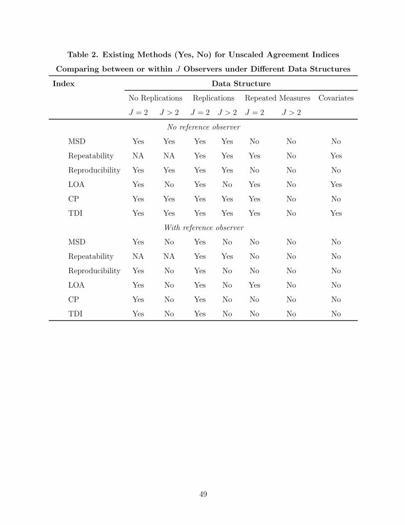
Table 2. Existing Methods (Yes, No) for Unscaled Agreement Indices
Comparing between or within J Observers under Different Data Structures
Index Data Structure
No Replications Replications Repeated Measures Covariates
J = 2 J > 2 J = 2 J > 2 J = 2 J > 2
No reference observer
MSD Yes Yes Yes Yes No No No
Repeatability NA NA Yes Yes Yes No Yes
Reproducibility Yes Yes Yes Yes No No No
LOA Yes No Yes No Yes No Yes
CP Yes Yes Yes Yes Yes No No
TDI Yes Yes Yes Yes Yes No Yes
With reference observer
MSD Yes No Yes No No No No
Repeatability NA NA Yes Yes No No No
Reproducibility Yes No Yes No No No No
LOA Yes No Yes No Yes No No
CP Yes No Yes No No No No
TDI Yes No Yes No No No No
49

Table 3. Existing Methods (Yes, No) for Scaled Agreement Indices
Comparing between or within J Observers under Different Data Structures
Index Data Structure
No Replications Replications Repeated Measures Covariates
J = 2 J > 2 J = 2 J > 2 J = 2 J > 2
No reference observer
ICC Yes Yes Yes Yes Yes Yes No
CCC Yes Yes Yes Yes Yes No Yes
CIA NA NA Yes Yes No No No
DC Yes Yes Yes Yes Yes Yes No
With reference observer
ICC No No No No No No No
CCC Yes Yes Yes Yes No No No
CIA NA NA Yes Yes No No No
DC No No No No No No No
Acknowledgments
This research is supported by the National Institutes of Health Grant R01 MH70028 (for
Huiman X. Barnhart and Michael Haber). We greatly appreciate Josep Carrasco and Pankaj
Choudhary for their timely review of this paper and their constructive comments that lead
to improvement of the content and completeness of the literatures in this paper.
Reference
American Educational Research Association (AERA), American Psychological Association
(APA), National Council on Measurement in Education (NCME). (1999) . The Stan-
dards for Educational and Psychological Testing. Washington, D.C.: American Psy-
chological Association.
Anderson, S., Hauck, W.W. (1990). Consideration of individual bioequivalence. Journal of
Pharmacokinetics and Biopharmaceutics 18: 259-273.
50
Atkinson, G., Nevill, A. (1997). Comment on the use of concordance correlation to assess
the agreement between two variables. Biometrics 53: 775-777.
Barnhart, H.X., Williamson, J.M. (2001). Modeling Concordance Correlation via GEE to
Evaluate Reproducibility. Biometrics 57:931-940.
Barnhart, H.X., Haber, M., Song, J. (2002). Overall concordance correlation coefficient for
evaluating agreement among multiple observers. Biometrics 58:1020-1027.
Barnhart, H.X., Song, J., Haber, M. (2005a). Assessing Assessing intra, inter, and total
agreement with Replicated Measurements. Statistics in Medicine 24: 1371-1384
Barnhart, H.X., Song, J., Lyles, R. (2005b). Assay validation for left censored data. Statis-
tics in Medicine 24: 3347-3360.
Barnhart, H.X., Haber, M., Kosinski, A.S. (2007a). Assessing Individual Agreement. Jour-
nal of Biopharmaceutical Statistics a special issue on agreement, in press.
Barnhart, H.X., Haber, M., Lokhnygina, Y., Kosinski, A.S. (2007b). Comparison of Con-
cordance Correlation Coefficient and Coefficient of Individual Agreement in Assessing
Agreement. Journal of Biopharmaceutical Statistics a special issue on agreement, in
press.
Bartko, J.J. (1966). The intraclass correlation coefficient as a measure of reliability. Psy-
chological Reports 19:3-11.
Bartko, J.J. (1974). Corrective note to “The intraclass correlation coefficient as a measure
of reliability”. Psychological Reports 34:418.
Bland, J. M., Altman, D. G. (1986). Statistical methods for assessing agreement between
two methods of clinical measurement. Lancet i: 307-310.
Bland, J.M., Altman, D.G. (1990). A note on the use of the intraclass correlation coefficient
in the evaluation of agreement between two methods of measurement. Computers in
Biology and Medicine 20:337-340.
51

Bland, J.M., Altman, D.G. (1992). This week’s citation classic: comparing methods of
clinical measurement. Current Contents CM 20(40) Oct 5:8.
Bland, J. M., Altman, D. G. (1995). Comparing methods of measurement: why plotting
difference against standard method is misleading. Lancet 346: 1085-1087.
Bland, J. M., Altman, D. G. (1999). Measuring agreement in method comparison studies.
Statistical Methods in Medical Research 8: 135-160.
Bland, J.M., Altman, D.G. (2007). Agreement between methods of measurement with
multiple observations per individual. Journal of Biopharmaceutical Statistics a special
issue on agreement, in press.
Brennan, R.L. (2001) Generalizability Theory. New York: Springer.
Carrasco, J.L., Jover, L. (2003a). Estimating the generalized concordance correlation coef-
ficient through variance components. Biometrics 59: 849-858.
Carrasco, J.L., Jover, L. (2003b). Assessing individual bioequivalence using the structural
equation model. Statistics in Medicine 22:901-912.
Carrasco, J.L., Jover, L. (2005a). The structural error-in-equation model to evaluate indi-
vidual bioequivalence. Biometrical Journal 47:623-634.
Carrasco, J.L., Jover, L. (2005b). Concordance correlation coefficient applied to discrete
data. Statistics in Medicine 24:4021-4034.
Carrasco, J.L., King, T., Chinchilli, V., Jover, L. (2007). Comparison of Concordance
Correlation Coefficient Estimating Approaches with Skewed Data. Journal of Bio-
pharmaceutical Statistics a special issue on agreement, in press.
Chen, M.L. (1997). Individual bioequivalence – A regulatory update. Journal of Biophar-
maceutical Statistics 7:5-11.
Chen, C., Barnhart, H.X. (2007). Comparison of ICC and CCC for assessing agreement for
data without and with replications. ENAR 2007 conference presentation in Atlanta,
GA.
52
Chinchilli, V.M., Martel, J.K., Kumanyika, S. Lloyd, T. (1996). A weighted concordance
correlation coefficient for repeated measures designs. Biometrics 52:341-353.
Choudhary, P.K. (2007a). A tolerance interval approach for assessment of agreement in
method comparison studies with repeated measurements. Journal of Statistical Plan-
ning and Inference submitted for publication.
Choudhary, P.K. (2007b). A tolerance interval approach for assessment of agreement with
left censored data. Journal of Biopharmaceutical Statistics a special issue on agree-
ment, in press.
Choudhary, P. K. (2007c) Semiparametric regression for assessing agreement using tolerance
bands. Computational Statistics and Data Analysis, in press.
Choudhary, P.K., Nagaraja, H.N. (2004). Measuring agreement in method comparison
studies - a review. In Advances in Ranking and Selection, Multiple Comparisons, and
Reliability, Balakrishnan, N,, Kannan, N., Nagaraja, H.N., eds., Boston: Birkhauser,
pp. 215-244.
Choudhary, P.K., Nagaraja, H.N. (2005a). Assessment of agreement using intersection-
union principle. Biometrical Journal 47:674-681.
Choudhary, P.K., Nagaraja, H.N. (2005b). Selecting the instrument closest to a gold stan-
dard. Journal of Statistical Planning and Inference 129:229-237.
Choudhary, P.K., Nagaraja, H.N. (2005c). A two-stage procedure for selection and assess-
ment of agreement of the best instrument with a gold-standard. Sequential Analysis
24:237-257.
Choudhary, P.K., Ng, H.K.T. (2006). Assessment of agreement under non-standard condi-
tions using regression models for mean and variance. Biometrics 62:288-296.
Choudhary, P.K., Nagaraja, H.N. (2007). Tests for assessment of agreement using proba-
bility criteria. Journal of Statistical Planning and Inference 137:279-290.
53

Cohen, J. (1960). A coefficient of agreement for nominal scales. Educational and Psycho-
logical Measurement 20:37-46.
Cohen, J. (1968). Weighted kappa: Nominal scale agreement with provision for scaled
disagreement or partial credit. Psychological Bulletin 70:213-220.
Cronbach, L.J., Gleser, G.C, Nanda, H., Rajaratnam, N. (1972). The dependability of
Behavioral Measurements: Theory of Generalizability for Scores and Profiles, New
York:Wiley.
Donner, A. (1998). Sample size requirements for the comparison of two or more coefficients
of inter-observer agreement. Statistics in Medicine 17:1157-1168.
Dunn, D. (1989). Statistical Evaluation of Measurement errors: Design and Analysis of
Reliability Studies. New York: Oxford University Press Inc.
Dunn, D. (1992). Design and analysis of reliability studies, Statistical Methods in Medical
Research 1:123-157.
Dunn, D. (2004). Statistical Evaluation of Measurement errors: Design and Analysis of
Reliability Studies. New York: Oxford University Press Inc.
Dunn, D. (2007). Regression models for method comparison data. Journal of Biopharma-
ceutical Statistics a special issue on agreement, in press.
Dunn, G., Roberts, C. (1999). Modelling method comparison data. Statistical Methods in
Medical Research 8:161-179.
Eliasziw, M., Young, S.L., Woodbury, M.G., Fryday-Field, K. (1994). Statistical method-
ology for the concurrent assessment of interrater and intrarater reliability: Using go-
niometric measurements as an example. Physical Therapy 74: 777-788.
Fagot, R.F. (1993). A generalized family of coefficients of relational agreement for numerical
scales. Psychometrika 58:357-70.
Fay, M.P. (2005). Random marginal agreement coefficients: rethinking the adjustment for
chance when measuring agreement. Biostatistics 6:171-180.
54

Fisher, R.A. (1925). Statistical methods for research workers. Edinburgh: Oliver and Boyd.
Fleiss, J.L. (1986). The Design and Analysis of Clinical Experiments, New York:Wiley.
Food and Drug Administration (FDA) (2001). Guidance for Industry: Bioanalytical Method
Validation, http://ww.fda.gov/cder/guidance/index.htm.
Galton, F. (1886). Family likeness in stature. Proceedings of the Royal Society 40:42-73.
Goodwin, L.D. (1997). Changing concepts of measurement validity. Journal of Nursing
Education 36:102-107.
Guo, Y., Manatunga, A.K. (2007). Nonparametric estimation of the concordance correla-
tion coefficient under univariate censoring. Biometrics in press.
Guttman, I. (1988). Statistical tolerance regions. In Encyclopedia of Statistical Sciences,
Vol. 9, Kotz, S., Johnson, N.L., eds., New York: Wiley, pp.272-287.
Haber, M., Barnhart, H.X., Song, J., Gruden, J. (2005). Observer variability: A new
approach in evaluating interobserver agreement. Journal of Data Science 3:69-83.
Haber, M., Gao, J., Barnhart, H.X. (2007). Assessing observer agreement in studies involv-
ing replicated binary observations. Journal of Biopharmaceutical Statistics a special
issue on agreement, in press.
Haber, M., Barnhart, H.X. (2006). Coefficients of agreement for fixed observers. Statistical
Methods for Medical Research 15:1-17.
Haber, M., Barnhart, H.X. (2007). A general approach to evaluating agreement between
two observers or methods of measurement. Statistical Methods for Medical Research in
press.
Hand, D.J. (2004). Measurement Theory and Practice. New York: Oxford University Press
Inc.
Harris, I. R., Burch, B. D., St. Laurent, R. T. (2001). A blended estimator for measure of
agreement with a gold standard. Journal of Agricultural, Biological and Environmental
Statistics 6:326-339.
55

Hawkins, D. M. (2002) Diagnostics for conformity of paired quantitative measurements.
Statistics in Medicine 21:1913-1935.
Hutson, A. D., Wilson, D. C., Geiser, E. A. (1998). Measuring relative agreement: Echocar-
diographer versus computer. Journal of Agricultural, Biological and Environmental
Statistics 3:163-174.
International Organization for Standardization (ISO) (1994). Accuracy (trueness and preci-
sion) of measurement methods and results – Part 1: general principles and definitions
(5725-1). Geneva, Switzerland: ISO.
Janson, H., Olsson U. (2001). A measure of agreement for interval or nominal multivariate
observations. Educational and Psychological Measurement 61:277-289.
Janson, H., Olsson U. (2004). A measure of agreement for interval or nominal multivariate
observations by different sets of judges. Educational and Psychological Measurement
64:62-70.
Kelly, G.E. (1985). Use of the structural equations model in assessing the reliability of a
new measurement technique. Applied Statistics 34:258-263.
King, T.S., Chinchilli, V.M. (2001a). A generalized concordance correlation coefficient for
continuous and categorical data. Statistics in Medicine 20: 2131-2147.
King, T.S., Chinchilli, V.M. (2001b). Robust estimators of the concordance correlation
coefficient. Journal of Biopharmaceutical Statistics 11:83-105.
King, T.S., Chinchilli, V.M., Carrasco, J. (2007a). A repeated measures concordance cor-
relation coefficient, Statistics in Medicine in press.
King, T.S., Chinchilli, V.M., Carrasco, J.L., Wang, K. (2007b). A class of repeated mea-
sures concordance correlation coefficients. Journal of Biopharmaceutical Statistics a
special issue on agreement, in press.
56

Krippendorff, K. (1970). Bivariate agreement coefficients for reliability of data. In Social
Methodology, Borgatta, B.F., Bohrnstedt, G.E., eds., San Francisco:Jessey-Bass, pp.
139-150.
Konishi, S. Khatri, C.G., Rao, C.R. (1991). Inferences on multivariate measures of interclass
and intraclass correlations in familial data. Journal of the Royal Statistical Society
series B 53:649-659.
Kraemer, H.C., Periyakoil V.S., Noda A. (2002). Kappa coefficients in medical research.
Statistics in Medicine 21, 2109-2129.
Lee, J., Koh, D., Ong, C. N. (1989). Statistical evaluation of agreement between two
methods for measuring a quantitative variable. Computers in Biology and Medicine
19:61-70.
Liao, J.J.Z. (2003). An improved concordance correlation coefficient. Pharmaceutical
Statistics 2:253-261.
Liao, J.J.Z. (2003). Agreement for curved data. Journal of Biopharmaceutical Statistics
15:195-203.
Lin, L.I. (1989). A concordance correlation coefficient to evaluate reproducibility. Biomet-
rics 45:225-268.
Lin, L.I. (1992). Assay validation using the concordance correlation coefficient. Biometrics
48:599-604.
Lin, L.I. (2000). A note on the concordance correlation coefficient. ıt biometrics, 56:
324-325.
Lin, L.I. (2000). Total deviation index for measuring individual agreement with applications
in laboratory performance and bioequivalence. Statistics in Medicine 19:255-270.
Lin, L.I. (2003). Measuring Agreement. In Encyclopedia of Biopharmaceutical Statistics,
Chow, S. eds., Philadelphia: Informa Healthcare, pp. 561-567.
57

Lin, L.I., Hedayat, A.S., Sinha, B., Yang, M. (2002). Statistical methods in assessing
agreement: Models, issues and tools. Journal of American Statistical Association 97:
257-270.
Lin, L.I., Hedayat, A.S., Wenting, W. (2007). A unfied approach for assessing agreement
for continuous and categorical data. Journal of Biopharmaceutical Statistics a special
issue on agreement, in press.
Lin, S.C., Whipple, D.M., Ho, C.S. (1998). Evaluation of statistical equivalence using limits
of agreement and associated sample size calculation. Communications in Statistics –
Theory and Methods 27: 1419-1432.
Liu X., Du Y., Teresi J., Hasin, D. S. (2005). Concordance correlation in the measurements
of time to event. Statistics in Medicine 24:1409-1420.
Lord, F.M., Novick, M.R. (1968). Statistical Theories of Mental Test Scores, Reading,
MA:Addison-Wesley.
McGraw, K.O., Wong, S.P. (1996). Forming inferences about some intraclass correlation
coefficients. Psychological Methods 1: 30-46.
Molenberghs, G., Vangeneugden, T., Laenen A. (2007). Estimating reliability and general-
izability from hierarchical biomedical data. Journal of Biopharmaceutical Statistics a
special issue on agreement, in press.
Muller, R., and Buttner, P. (1994). A critical discussion of intraclass correlation coefficients.
Statistics in Medicine 13:2465-2476.
Nickerson, C. A. (1997) Comment on ”A concordance correlation to evaluate reproducibil-
ity”. Biometrics 53:1503-1507.
Pearson, K. (1896). VII. Mathematical contributions to the theory of evolution — III.
Regression, heredity and panmixia. Philosophical Transactions of the Royal Society,
Series A 187:253-318.
58
Pearson, K., Lee, A., Bramley-Moore, L. (1899). VI. Mathematical contributions to the
theory of evolution. — VI. Genetic (reproductive) selection: Inheritance of fertility in
man, and of fecundity in thoroughbred racehorses. Philosophical Transactions of the
Royal Society, Series A 192:257-330.
Pearson, K. (1901). VIII. Mathematical contributions to the theory of evolution. — IX.
On the principle of homotyposis and its relation to heredity, to the variability of the
individual, and to that of the race. Part I. Homotyposis in the vegetable kingdom.
Philosophical Transactions of the Royal Society, Series A 197:285-379.
Raghavachari, M. (2004). Measures of concordance for assessing agreement in ratings and
rank order data. In Advances in Ranking and Selection, Multiple Comparisons and
Reliability, Balakrishnan, N., Kannan, N., Nagaraja, H. N., eds., Boston:Birkhauser,
pp. 245-263.
Robieson, W. (1999). On weighted kappa and concordance correlation coefficient. Ph.D.
thesis, University of Illinois in Chicago.
Quan, H., Shih, W.J. (1996). Assessing reproducibility by the within-subject coefficient of
variation with random effects models. Biometrics 52:1195-1203.
Quiroz, J. (2005). Assessment of equivalence using a concordance correlation coefficient in
a repeated measurement design. Journal of Biopharmaceutical Statistics 15:913-928.
Ryan, T.P., Woodall, W.H. (2005). The most-cited statistical papers, Journal of Applied
Statistics 32:461-474.
Shao, J., Zhong, B. (2004). Assessing the agreement between two quantitative assays with
repeated measurements. Journal of Biopharmaceutical Statistics 14:201-212.
Shavelson, R.J., Webb, N. M. (1981). Generalizability: 1973-1980. British Journal of
Mathematical and Statistical Psychology 34: 133-166.
Shavelson, R.J., Webb, N. M., Rowley, G. I. (1989). Generalizability theory. American
Psychologist 44: 922-932.
59
Shavelson, R.J., Webb, N. M. (1991). Generalizability Theory: A Primer. Newbury Park,
CA: SAGE Publication.
Shavelson, R.J., Webb, N. M. (1992). Generalizability theory. In M. C. Alkin (ed.), Ency-
clopedia of Education Research (Vol.2, pp. 538-543), New York: Macmillan.
Shoukri, M.M. (1998). Measurement of agreement, In the Encyclopedia of biostatistics, P.
Armitage, T. Colton, eds., New York:Wiley, pp. 102-116.
Shoukri, M.M., Asyali, M.H., Donner, A. (2004). Sample size requirements for the design
of reliability study: review and new results. Statistical Methods in Medical Research
13: 251-271.
Shrout, P.E. (1998). Measurement reliability and agreement in psychiatry. Statistical Meth-
ods in Medical Research 7:301-317.
Shrout, P. E., Fleiss, J. L.(1979). Intraclass correlations: uses in assessing rater reliability.
Psychological Bulletin 86: 420-428.
St. Laurent, R.T. (1998). Evaluating agreement with a gold standard in method comparison
studies. Biometrics 54:537-545.
Stine, W.W. (1989) Interobserver relational agreement. Psychological Bulletin 106:341-7.
Vangeneugden, T., Laenen, A., Geys, H., Renard, D., Molenberghs, G. (2004). Applying
linear mixed models to estimate reliability in clinical trials with repeated measure-
ments. Controlled Clinical Trials 25:13-30.
Vangeneugden, T., Laenen, A., Geys, H., Renard, D., Molenberghs, G. (2005). Apply-
ing concepts of generalizability theory on clinical trial data to investigate sources of
variation and their impact on reliability. Biometrics 61:295-304.
Wang,W., Hwang, J.R.G. (2001). A nearly unbiased test for individual bioequivalence
problems using probability criteria. Journal of Statistical Planning and Inference 99:41-
58.
60

Williamson, J.M., Crawford, S. B., Lin, H. (2007). Permutation testing for comparing
dependent concordance correlation coefficients. Journal of Biopharmaceutical Statistics
a special issue on agreement, in press.
Zhong, B., Shao, J. (2003). Evaluating the agreement of two quantitative assays with
repeated measurements. Journal of Biopharmaceutical Statistics 13:75-86.
Zegers, F.E. (1986). A family of chance-corrected association coefficients for metric scales.
Psychometrika 51:559-62.
61