An Overview of Pricing Models for Revenue Management

Gabriel Bitran∗ Rene Caldentey†

December, 2002

Abstract

In this paper we examine the research and results of dynamic pricing policies and their rela-tion to Revenue Management. The survey is based on a generic Revenue Management problemin which a perishable and non-renewable set of resources satisfy stochastic price-sensitive de-mand processes over a finite period of time. In this class of problems, the owner (or the seller)of these resources uses them to produce and offer a menu of final products to the end customers.Within this context, we formulate the stochastic control problem of capacity that the sellerfaces: how to dynamically set the menu and the quantity of products and their correspondingprices in order to maximize the total revenue over the selling horizon.

1 Introduction

The aim of this paper is to review the growing literature on Dynamic Pricing Policies and itsconnection to Revenue Management. In general terms, the Revenue Management model that weinvestigate considers the problem faced by a seller who owns a fixed and perishable set of resourcesthat are sold to a price sensitive population of buyers. In this framework where capacity is fixed,the seller is mainly interested in finding an optimal pricing strategy that maximizes the revenuecollected over the selling horizon.The motivation for this work is our strong belief that pricing policies are today, more than everbefore, a fundamental component of the daily operations of manufacturing and service companies.The reason is probably because price is one of the most effective variables that managers canmanipulate to encourage or discourage demand in the short run. Price is not only important froma financial point of view but also from an operational standpoint. It is a tool that helps to regulateinventory and production pressures. Airline companies and retail chains are good examples ofindustries where dynamic pricing policies are becoming key drivers of the companies’ performance.Not surprisingly, pricing models have become increasingly popular within the Management Sciencecommunity. Researchers have realized that classical operational problems such as optimal capacityand inventory management or controlling congestion in a queueing network, among many others,cannot be decoupled from marketing activities and especially pricing decisions. This broad rangeof applications has generated an important volume of work. We believe it is time to survey thefield and to present the main results and their practical implications. We do not attempt, however,an exhaustive review of the vast literature on pricing. Instead we focus on the work that has beendone in the context of Revenue Management.

∗Sloan School of Management, MIT, Cambridge, MA 02139, (617) 253-2652 Fax: (617) 258-7579, gbitran@mit.edu†Stern School of Business, New York University, New York, NY 10012, (212) 998-0298, Fax: (212) 995-4227,

rcaldent@stern.nyu.edu

The rapid evolution of information technologies and the corresponding growth of the Internet andE-commerce are sources of inspiration for a survey on dynamic pricing models for two main reasons.First, in this electronic world, it is possible to collect valuable information (about demand, inventorylevels, competitors strategies, etc.) and process it in real time. This new reality allows –and forces–managers to act and react dynamically to changes in the marketplace by adjusting any variableunder control, especially prices. Furthermore , Internet based selling systems make the logistics ofdynamic pricing much easier. The costs associated with relabelling the prices of the products andinforming customers about these changes have dropped significantly in the electronic environmentwhen compared to traditional brick and mortar businesses (e.g. Brynjolfsson and Smith [18]). Onthe customer side, Internet price search intermediaries or web aggregators offer customers easyaccess to better information about product variety and price lists (e.g., priceline.com). As a result,new potential applications for Revenue Management techniques are emerging in connection to theInternet. We consider it important to present the fundamental aspects of dynamic pricing modelsto an audience that is currently working and developing E-commerce.From a historical perspective, the interest in Revenue Management practices started with thepioneering research of Rothstein [69]-[70] and Littlewood [52] on airline and hotel overbooking.However, it was probably after the work of Belobaba [6]-[8] and the American Airlines success [72]that the field really took off. The airline industry provided researchers with a concrete example ofthe tremendous impact that Revenue Management tools can have on the operations of a company(e.g., Smith et al. [72]). The publication of a survey paper by Weatherford and Bodily [83], wherea taxonomy of the field and an agenda for future work were proposed, was another symptom ofthis revival. At this stage, however, much of the work was done on capacity management and over-booking with little discussion of dynamic pricing policies. In essence, prices (fares) in these originalmodels were assumed to be fixed and managers were in charge of opening and closing differentfare classes as demand evolved. During the 90’s, the increasing interest in Revenue Managementbecome evident in the different applications that were considered. Models became industry specific(e.g. airlines, hotels, or retail stores) with a higher degree of complexity (e.g. multi-class and multi-period stochastic formulations). Furthermore, it was in the last decade that pricing policies reallybecame an active component of the Revenue Management literature (e.g., Gallego and van Ryzin[36], Bitran and Mondschein [15], Feng and Gallego [27]-[28]). Today, dynamic pricing policies ina Revenue Management context is an active field of research that has reached a certain level ofmaturity.In terms of applications, dynamic pricing practices are particularly useful for those industries havinghigh start-up costs, perishable capacity, short selling horizons, and a demand that is both stochasticand price sensitive. Succinctly, the Revenue Management problem has been phrased as “selling theright product to right customer at the right time”. On one hand, the sellers would like to sell theirproducts to those customers having a high valuation so that high margins can be achieved. On theother hand, if they wait too long for those high valuation customers to appear, they might end theselling period with unsold units that could have been sold to low valuation customers. Clearly, forthis trade off to be non trivial, both perishable capacity and stochastic demand are needed. Aswe will discuss in this paper, it is precisely in this environment that dynamic pricing strategies areespecially useful to balance utilization and profitability of the available capacity.As we already mentioned, the airline industry pioneered the use of Revenue Management techniquesin terms of capacity/seat control and dynamic pricing. Today, Revenue Management has spreadout naturally to other industries such as retailers (e.g. Bitran and Mondschein [15], Subrahmanyanand Shoemaker [75]), car rental agencies (e.g. Carol and Grimes [19], Geraghty and Johnson

2

[39]), hotels (e.g., Bitran and Mondschein [12]), Bitran and Gilbert [14]), bandwidth and Internetproviders (e.g., Nair and Bapna [62]), passenger railways (e.g., Ciancimino et al. [21]), cruise lines(e.g., Ladany and Arbel [48]), electric power supply (e.g., Schweppe [71], Smith [73], Oren andSmith [63]). Although different in many respects, these industries all share the basic propertiesof the Revenue Management problems that we consider in this work, namely, perishable products,finite selling horizons, and price sensitive and stochastic demand.We conclude this introduction by positioning this paper with respect to other similar works thathave been published. In terms of goals, our objective is to present the main results that havebeen reported in the literature during the last decades on dynamic pricing models. We concentrateour efforts on understanding the main drivers and properties of optimal pricing strategies. Inthis respect, we do not discuss in detail the somewhat related research that has been done inthe area of inventory and capacity control, although some related results for network RevenueManagement problems are presented in section §3.2.2. Our work differs from other survey paperssuch as Weatherford and Bodily [83] or McGill and van Ryzin [56] since we do not attempt toprovide a taxonomy or an exhaustive enumeration of all the publications in the field. Similar inmany aspects to our work is the survey on dynamic pricing models by Elmaghraby and Keskinocak[26] where a broad view of the field is presented from a set of different angles such as pricing policiesfor long and short life cycle products, or combined inventory and pricing decisions, or pricing inmarkets with rational customers. However, we preferred to narrow the scope of our work to dynamicpricing models in a Revenue Management context so that we can explicitly present and discuss themain results that have been obtained. In this regard, we believe that our work provides a helpfulsummary of this field to those readers (researchers or practitioners) interested in getting a generaloverview of the research that has been done thus far. Nevertheless, we believe that a good surveyshould not only introduce the field and main results to the nonspecialists but also provide newinsights and guidance for future research to the experts. For this purpose, we have complementedour review with some new results, and we have included a list of potential new directions of researchin section §4.The remainder of this paper is organized as follows. We develop in section §2 a generic formulationof the Revenue Management problem that provides a global view of the different elements and theirinterrelationship. In particular, we present a general pricing problem and describe how the differentcomponents such as demand attributes, product characteristics, information, and constraints affectthe formulation and its applicability. Next, in section §3 we review the literature and the mainresults. We approach this review from different angles such as deterministic versus stochasticmodels and single versus multi products models. Finally, in section §4, we summarize our resultsand identify open problems and new potential directions of research.

2 A Generic Model

In this section, we describe the Revenue Management model under consideration. The model thatwe present is sufficiently general to cover the research that we review in section §3 as a specialcase. Furthermore, some of the elements of our generic formulation in §2.6 have not yet been fullyaddressed in the literature. In this respect, our motivation for this apparent excess of generality istwofold. First of all, we believe that our generic framework is more appealing to those nonspecialistreaders interested in getting the “big picture” behind the Revenue Management problem. Secondly,the contrast between this general model and the specific research presented in §3 can be used toidentify potential research opportunity. In section §4, we suggest some new directions.

3

2.1 Supply

Consider a seller or market player (e.g., an airline, hotel, car rental company, retail store, or anInternet service provider) which has a fixed amount of initial capacity that is used to satisfy aprice-sensitive demand† during a certain selling period H = [0, T ]. We model this initial capacityas an m-dimensional vector C0 = (c1(0), . . . , cm(0)) of resources where ck(0) is the initial amount ofresource k available. Capacity, in our context, is a rather broad concept that might include numberof rooms in a hotel, available seats for a specific origin-destination flight in a given day, or simplythe number of white shirts in stock at a garment store.Under the “standard” Revenue Management problem that we consider, capacity is fixed and anystrategic considerations regarding how to acquire the initial level C0 have been excluded. Capacityis essentially given and the seller is committed exclusively to finding the best way to sell it. Thisassumption is by no means critical if we consider that in many industries capacity is flexible only inthe long run. Moreover, capacity decisions and price decisions take place on different time scales.Issues regarding the size of a hotel or an airplane or the number of shirts to purchase from anoverseas supplier are decided long before demand is realized and price policies are implemented.Critical to the revenue management problem are the characteristics of this available capacity andhow it is used to create a set (or menu) of final products. As we will see shortly, in some casesmuch of the complexity of the revenue management problem comes from selecting the correct menuof products. From a pricing perspective, two important attributes of the available capacity are itsdegree of flexibility and its perishability.

Flexibility measures the ability to produce and offer different products using the initial capacityC0. We say that capacity is dedicated if there is a one-to-one correspondence between capacity andfinal product. For example, a retailer that purchases 500 white T-shirts to sell during the nextsummer season has dedicated capacity. On the other hand, we say that capacity is flexible if itcan be used to produce different products or satisfy different customers’ needs. For example, anInternet provider owning bandwidth capacity uses this specific resource to offer a wide range ofproducts from email services to video conferences. In general, flexibility is a continuous attributeranging from highly dedicated (retailing) to highly flexible (the bandwidth provider).It should be intuitively obvious that flexibility is a desired feature. In essence, flexible capacityallows the seller to allocate scarce resources efficiently based on observed demand rather than fore-casted demand (production postponement). In practice, however, flexibility is not always possible.A retailer buying from an overseas supplier needs to order months before the beginning of theselling season. In the hotel industry, the allocation of the available space into luxury, suite, andstandard rooms is essentially decided when the hotel is built.From a pricing standpoint, flexibility increases the complexity of the problem. As we will discusslater, the action of selling a product has associated two quantities: (i) an immediate revenue equalto the price and (ii) an opportunity cost which is the monetary penalty of using capacity today thatcould be used to satisfy future demand. When capacity is dedicated, selling product i does not affectthe ability to supply product j. Thus, the opportunity cost of selling i involves essentially producti and its demand. However, when capacity is flexible selling product i decreases the resourcesavailable to produce product j. This interaction among products makes the computation of theopportunity cost and the optimal pricing strategy much harder.

Perishability relates to the (lack of) ability to preserve capacity over time. For example, an

†Demand can also depend on other variables controlled by the seller like capacity itself.

4

empty seat on a departing flight is a unit of capacity that cannot be stocked for a future flight.In general, a distinctive feature of the Revenue Management problem is the perishability of theavailable capacity. A simple way to treat this perishability is making capacity a time-dependentquantity. For instance, a hotel’s unit of resource might be “Room 106 on Friday night, May 10,2002” while an airline’s unit of capacity could be “Seat 22B on flight #1243 departing from Bostonto Chicago at 4:00pm on Tuesday, May 14, 2002”. How much detail is used to define the unitsof capacity depends on customers’ preferences and the seller’s ability to profit from their choice.For example, two economic-class seats 22A (window) and 22B (aisle) on a given flight could beconsider two different resources and priced differently if customers have significant differences ontheir preferences for window and aisle seats. In practice, airlines do not discriminate based on thisfeature and both seats 22A and 22B are considered two units of the same resource: economy-classseats. Retailers, on the other hand, are much more active in this way, charging different prices fora blue shirt and for a red shirt (same model, brand, and size).From a modelling perspective, perishability increases the dimension of the problem, making capac-ity, and therefore final products, time-dependent quantities. In our dynamic setting, perishabilityis an inherent property of the model, although it might be irrelevant in some cases, e.g., whencapacity is fully inventoriable and the selling horizon goes to infinity.As time progresses and resources are consumed (they are sold or they perish), capacity decreasesand we denote by Ct = (c1(t), . . . , cm(t)) the available capacity at time t.

2.2 The Product

Following our previous description of capacity, a product in this context is a sub-collection of theavailable resources. Based on Gallego and van Ryzin’s [37] production model, we consider an m×nmatrix A = [aij ] such that aij represents the amount of resource i used to produce one unit ofproduct j. That is, every column j of A represents a different product –say product A·j– and thecollection M = {A·1, . . . , A·n} is the menu of products offered by the seller. We will consider forthe moment that there is no explicit costs associated to the production of the final products. Thisis, by the way, a common assumption in the literature. In many situations, this assumption is notvery restrictive since production costs are negligible, or they are linear and can be incorporateddirectly into the final price.Given the available initial capacity C0 the first important decision of the seller is to define the menuM of products that will be offered to the end customers. A naıve approach would be to considerany possible subset of C0 as a product, i.e., M = {a ∈ IRm : 0 ≤ a ≤ C0}. However, even if ademand exists for every conceivable subset of C0, the task of setting a different price strategy forevery combination is computationally demanding and hard to implement. On one hand, managinga short list of products simplifies the pricing problem. On the other hand, a larger list is moresuitable for demand-skimming purposes. The right mix of products should balance this trade-off.For instance, the simplest approach would be to set A = Ik, the (k × k) identity matrix. In thiscase, every resource is dedicated and offered as a single product. Customers are left with the taskof purchasing the appropriate combination of each resource depending on their specific needs. Inthis case a minimum set of prices is needed, one for each resource. The seller, however, can try todo better by creating bundles, which are specific subsets of resources that match specific customers’needs. By doing so, the seller is able to target the market and increase demand. In this case, alarger set of prices has to be specified with the corresponding increment in management costs.

5

2.3 Information

Crucial to any dynamic pricing policy is the knowledge of the system and its evolution over time.Real-time pricing necessarily requires real-time demand data, the available capacity, and any otherrelevant factors (e.g., competitors’ strategies, weather). Thus, an information system capable ofcollecting the right information and making it available at decision points is critical. There islittle doubt that one of the major factors that influenced the rapid growth of Yield Managementin the airline industry was the development of electronic information systems capable of gatheringinformation about demand and ticket reservation over the large network of travel agencies (e.g.,SABRE system for American Airlines, Smith et al. [72]). Similarly, as reported by Raman et al.[66], retailers are investing large amounts of money (close to $30 billion a year) to improve ITsystems and reduce the systematic problem of inaccurate inventory records.In our Revenue Management setting, short product life-cycles and perishability impose extra pres-sure to improve the quality and management of information such as demand forecast and inventoryposition. For instance, standard forecast methods rely heavily on demand history that is notnecessarily available in this short life-cycle environment, for example, retailers selling fashionableproducts (e.g., Fisher and Ramana [35], Kurawarwala and Matsuo [55]).Given an initial capacity C0, a product menu M, and a demand and price processes, we definethe observed history Ht of the selling process as the set of all relevant information available up tot. This history should include at least the observed demand process and available capacity, andit can also include some additional information such as demand forecasts. Most of the researchhas focused on the simple but tractable Markovian case where Ht = Ct, in which only remainingcapacity is relevant for pricing decisions. However, path-dependent models are specially usefulwhen demand distribution is unknown and a learning process is incorporated to improve demandestimates. In general, we expect some degree of information asymmetry between the seller andthe buyers. Issues regarding the quality of the product or the level of inventory, for instance, areusually private information held by seller. On the other hand, customers have private informationabout their product valuations and budget. This asymmetry of information can be modelled usingtwo sub-histories Hs

t ,Hbt ⊆ Ht representing the information available to the seller and customers,

respectively, at time t.

2.4 Demand

On the demand side, we divide the set of potential customers into different segments each onehaving its own set of attributes including needs, budget, and quality expectations. We definea d-dimensional stochastic process N(t,Ht) = (N1(t,Ht), . . . , Nd(t,Ht)) where Nj(t,Ht) is thecumulative potential demand up to time t from family j given the available information Ht.Depending on the price (and probably other attributes such as quality) potential customers willdecide whether or not to purchase the products. Using Lazear [49] terminology, potential customersare divided into (i) shoppers which are those customers that search for products but do not buybecause of price or quality considerations and (ii) buyers which are those customers that areeffectively willing to buy a product. In general, pricing policies should be computed on the basesof both potential customers and buyers. However, in most applications the seller is only capable ofcollecting information about the set of buyers according to sales data‡.

‡One exception is the catalog industry, here the seller controls the population of potential consumers according tothe mailing policy (e.g., Bitran and Mondschein [14]). E-commerce is another example since information on shoppers(as opposed to buyers) can be obtained via the Internet, by storing the path customers follows on the website.

6

In order to model this purchasing process, we define an n × d matrix B(P ) = [bij ] where bij

represents the units of product i ∈ M requested by a customer in family j = 1, . . . , d; the priceprocess Pt = {ps : s ∈ [0, t]} is described in detail in section §2.5 below. It is important to notethat bundling considerations are directly linked to the structure of this matrix B(P ) through itsdependence on the product menu M. Combining the vector of potential demand N(t,Ht) and thematrix B(P ), we define an n-dimensional vector D(t, P,H) ≡ B(P ) N(t,Ht) that represents theeffective cumulative demand process in [0, t] at the product level.Finally, we provide the seller with the ability to partially serve demand if it is profitable to do so.For instance, retailers do not display their entire inventory during promotion days. In the same way,airlines are able to reject low-fare reservations (closing a fare) even if they have available capacity.In light of this, we define an n-dimensional vector S(t) that represents the cumulative sales up totime t. Given the demand, sales, and price processes, the dynamics of the available capacity aregoverned by the following conditions.

Ct = C0 −A S(t) and S(t) ≤ D(t, P,Ht) for all t ∈ [0, T ]. (1)

In some contexts, the distinction between sales S and demand D is unnecessary. For instance,if the price can be adjusted continuously and unrestrictedly, the seller will prefer to increase theprice rather than reject customers. In this case, the price is the only variable that the seller needsto control. For example, in the yield management literature of seat control, the notion of a nullprice§ has been introduced to model the accept/reject decision in the context of dynamic pricingpolicies (see section §3.2.2). We note that if the seller is constrained in the way that s/he canadjust the price (see §2.5 below for some examples of constraints) then the distinction betweensales and demand becomes relevant and the accept/reject decision is not necessarily replicableusing a dynamic pricing strategy.In terms of our assumptions, the use of a price-sensitive demand D(t, P,Ht) implies that theseller has monopolistic market power over the set of buyers. Competition might be present in thisformulation, but it is hidden and only the residual demand N(t,Ht) faced by the seller is considered.We do not incorporate any strategic behavior from the customers’ side, demand might depend onthe whole observed history of the selling process but we do not model the utility maximizationprocess solved by the customers. Demand in this respect is assumed to be given exogenously.Similarly, customers are assumed to be price takers, meaning they observe the price list offered bythe seller and react by buying or not buying some of the products. We will postpone the discussionof other allocation mechanisms such as auction models to section §4.Certainly, good modeling and forecasting of demand are key for pricing purposes. The alternativeformulations available in the literature are unlimited especially in the deterministic demand case.The simplest approach is probably to decompose this deterministic demand into a set of differentfactors, each one addressing a specific aspect of the problem (e.g., Eliashberg and Jeuland [25],Kalish [44], Jain and Rao [42]):

Ddet(t, p,Ht) = D(t)G(p)F(Ht), (2)

where D(t) is an estimate of the market size as a function of time, G(p) captures price elasticityeffects, and F(Ht) models the influence of the available information on customers’ purchasingbehavior.From micro economics theory (e.g. Mas-Colell et al. [54]), the notions of consumers’ utility,elasticity, and product substitution form the bases of our understanding and modeling of G(p). For

§A high price that makes demand equal to zero almost surely.

7

example, exponential demand models are commonly used to model demand in the retail sector (e.g.,Smith and Achabal [74]). That is, G(p) = exp(−ηp), where η is a measure of demand elasticityper unit of price. Other models using constant elasticity, G(p) = p−η, have also been proposed(e.g., Bitran et al. [16]). A functional form for F(Ht), for the case Ht = Ct, was developed andempirically tested in Smith and Achabal [74].On the other hand, the modeling of D(t) depends on the seasonality of demand and the life cycle ofthe product. Diffusion models (e.g., Bass [3]) are widely used to model this evolution of demand.In this framework, a population of consumers of size N gradually purchases the product. The rateat which consumers buy the product depends linearly on the number of previous purchases (word-of-mouth or diffusion effects) and the fraction of innovators existing in the population. Innovatorsare those consumers that buy the product independently of the other consumers’ actions. In Bass’s[3] diffusion model, the rate of purchase at time t is given by

dD(t)dt

= pN + (q − p)D(t)− q

ND2(t), (3)

where p is the fraction of innovators and q is a measure of the diffusion effect (imitation). Thecombination of this diffusion model with price has been proposed in Bass [4] and Jeuland andDoland [43].The stochastic behavior of the demand has been added to these deterministic models for discrete andcontinuous time formulations. For the discrete time case, the standard approach is to representdemand as the sum of a deterministic part and a zero-mean stochastic component. Using thenotation dD(t, p,H) for the marginal demand in period t, the stochastic additive noise model isgiven by

dDstoc(t, p,Ht) = dDdet(p, t,Ht) + ξ(t, p,Ht)︸ ︷︷ ︸Random Noise

. (4)

The random noise, which usually follows a zero-mean normal random variable, depends on priceand time to reflect the changes on demand uncertainty over the life cycle. Another alternativemodel is the multiplicative noise model

dDstoc(t, p,Ht) = dDdet(t, p,Ht) ξ(t, p,Ht). (5)

In this case, the expected value random noise is normally set to one. Combinations of the additiveand multiplicative models can also be used.For the continuous time case, the most common formulation assumes that demand follows a Poissonprocess with a deterministic intensity that depends on price and time (e.g., Gallego and van Ryzin[36]-[37], Bitran and Mondschein [15], Feng and Gallego [28]), although it is possible to extend thediscrete time formulation above replacing the normally distributed random noise by a continuoustime Wiener process (e.g., Raman and Chatterjee [67]).

2.5 Pricing Strategies

In our dynamic setting, a pricing policy P := PT = {pt : t ∈ [0, T ]} is a collection of mappingspt(·|Ht) : M→ IR+ where pt(i|Ht) is the price of product i ∈ M at time t given a current historyHt. Depending on the application, some conditions have to be imposed to ensure that the resultingpricing policy P is consistent with standard practices in industry. The following is a list of themost common constraints that we have come across during our literature review and industrialexperience.

8

• Finite set of prices: In many applications the seller can only select prices from a finite listof admissible prices, i.e., Pt = {p1, . . . , pKt} (e.g., Chatwin [20], Feng and Xiao [30]-[31],Feng and Gallego [28]). The reasons range from marketing considerations such as customers’perception of prices ($19.99 versus $20.00) to managerial aspects since a discrete list of pricesis easy to implement and control.

• Maximum number of price changes: Most companies restrict the number of price changesduring the selling horizon (e.g. Feng and Gallego [27]). In some cases, this restriction is notcritical since two-price policies have been shown to be asymptotically optimal (e.g., Gallegoand van Ryzin [36]). In practice, companies restrict the number of price changes becausechanging prices too often is difficult and costly from an operational standpoint. We shouldmention, however, that for the growing Internet-based sale systems, the costs of relabellingthe prices of products and those associated with informing customers about these changesare dropping considerably (e.g. Brynjolfsson and Smith [18]).

• Markdowns, Markups, and Promotions: It is common practice in some industries to enforce apredefined path of the price over time. For instance, retailers usually adopt a markdown pol-icy, or clearance policy, that makes the prices of the products to decrease monotonically overtime (e.g., Bitran and Mondschein [15]). In general, these markdown policies are appropriatefor those industries which face customers whose willingness to pay for the product diminishesover the selling season such as the retailing. On the contrary, airline companies prefer tomark up their prices in order to discriminate among travellers and business passengers. Inthis case, customers’ willingness to pay increases over time since the more profitable businesssegment tends to make last minute travel arrangements. Markdowns or markups are rarelyadvertised, and customers become aware of these variations only through past experiences andword-of-mouth. Promotions, on the other hand, are discounts that companies offer at specificmoments in time (such as Mother’s Day). These discounts are advertised and reversible.

• Joint Price Constraints: In some situations, different products cannot be priced independently.This happens naturally with bundles since the price of the bundle should depend on theprice of the different components. For instance, there are practical issues, such as marketingconsiderations or competitors’ strategies, that can force the price of the bundle to be at leastx% (say 10%) cheaper than the sum of the price of the components. In this case, if producti ∈ M is a bundle resulting from packing together all the products j ∈ Bi ⊆ M, then thebundling constraint on the price is as follows.

pt(i) ≤ x∑

j∈Bi

pt(j) for all t ∈ [0, T ]. (6)

Another case where joint price constraints arise naturally is when the same product is offeredat different locations that have independent demand. In this case, it can be argued that theproduct in location k is different than the product in location l because they face differentdemand processes and therefore a different price can be set at each location. In practice,however, companies try to avoid this type of geographical discrimination because of imageand reputation issues (Bitran et al. [16]). In this case, the functional constraint that is addedto the model is

pt(k) = pt(l) for all t ∈ [0, T ]. (7)

Joint price constraints can also occur over time. For example in some industries price is forcedto follow a monotonic path. The path might be decreasing, such as permanent markdowns

9

in the retail sector (Mantrala and Surya [53]), or increasing as it happens in the airlineindustry. In general, most companies try to avoid pricing policies that may be viewed as“unfair” by the end customers. Situations where two first-class passengers seated togetherafter having paid significantly different prices for their seats can have a negative impact oncustomers’ perception (especially for the passenger having the expensive ticket). To minimizethis problem, the airline company could consider pricing policies that satisfy the followingcondition.

pt − ps ≤ ξ for all t, s ∈ [0, T ], (8)

where ξ is an upper bound on the variability of the pricing policy.

• Cost-Based Pricing: Although capacity is a sunk cost in our setting and in most of the appli-cations that we consider, there is still some tendency in practice to set prices based on costs.The reason is probably a mixture of managers’ incentives based on margins and the classicaladvice from economic theory where marginal cost plays a central role in pricing decisions. Itshould be intuitively obvious, however, that once capacity is determined, then pricing policiesshould only try to maximize the revenue without any cost consideration (except for produc-tion costs that we have assumed are negligible). In some cases, however, there are legalrestrictions to price below cost, and so cost-based pricing is exogenously imposed. A simplecost-based pricing constraint (that we have come across working in the apparel industry) isgiven by pt ≥ (1 + x) r, where r is the unit cost of the product and x is a minimum margincontribution imposed on the product. Note that if x and r are fixed, then we can redefinethe price as pt ← pt − (1 + x) r. Under this net margin price formulation, the cost-basedconstraint above reduces to the nonnegativity of the pricing policy which is always satisfiedin our revenue maximization context.

In general, we will denote by P the set of all admissible pricing policies, those that satisfy all therelevant constraints.

2.6 Revenue Management Formulation

Given the available capacity C0, the cumulative demand process N(t), the menu of available prod-ucts M, and a set of admissible policies P, the seller’s objective is to find a pricing strategy Pt

that maximizes the total revenue collected from selling the products to the customers. In addition,the seller has the ability to partially serve demand, and so the selling process St is also part of thedecision variables. The problem faced by the seller is to find the solution to the following optimalcontrol problem.

supP,S

EN

[∫ T

0pt dS(t)

](9)

subject to: Ct = C0 −AS(t) ≥ 0 for all t ∈ [0, T ], (10)0 ≤ S(t) ≤ D(t, P,Ht) for all t ∈ [0, T ], (11)P ∈ P, and S(t) ∈ Ht. (12)

We first note that the model corresponds to a revenue maximization problem. The objective (9)is simply the expected revenue collected from selling the products over the available selling period[0, T ]. As we mentioned in §2.1 all considerations associated with acquiring the initial level ofcapacity C0 have been excluded.

10

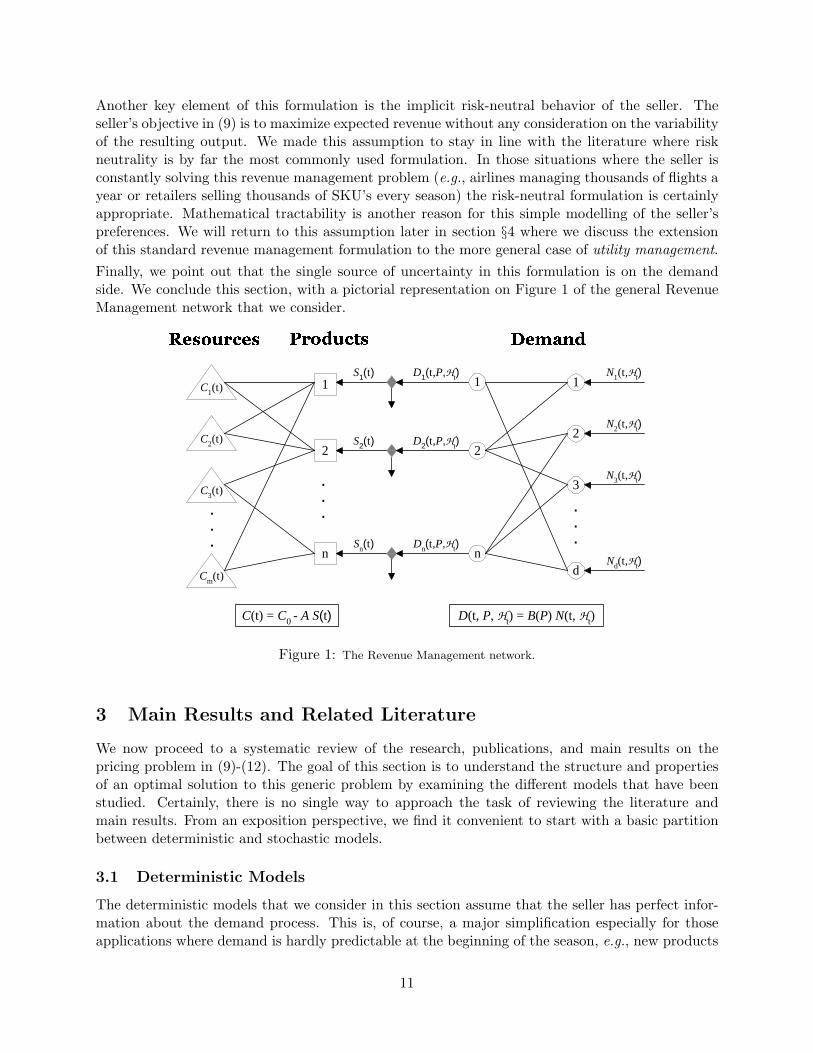
Another key element of this formulation is the implicit risk-neutral behavior of the seller. Theseller’s objective in (9) is to maximize expected revenue without any consideration on the variabilityof the resulting output. We made this assumption to stay in line with the literature where riskneutrality is by far the most commonly used formulation. In those situations where the seller isconstantly solving this revenue management problem (e.g., airlines managing thousands of flights ayear or retailers selling thousands of SKU’s every season) the risk-neutral formulation is certainlyappropriate. Mathematical tractability is another reason for this simple modelling of the seller’spreferences. We will return to this assumption later in section §4 where we discuss the extensionof this standard revenue management formulation to the more general case of utility management.Finally, we point out that the single source of uncertainty in this formulation is on the demandside. We conclude this section, with a pictorial representation on Figure 1 of the general RevenueManagement network that we consider.

1

2

n

.

.

.

.

.

.

������������ ���������

C1(t)

.

.

.

������ ����������

C2(t)

C3(t)

Cm(t)

D1(t,P,Ht)S1(t)

D2(t,P,Ht)S2(t)

Dn(t,P,Ht)Sn(t)

1

2

n

1

2

3

d

N1(t,Ht)

N2(t,Ht)

N3(t,Ht)

Nd(t,Ht)

C(t) = C0 - A S(t) D(t, P, Ht) = B(P) N(t, Ht)

Figure 1: The Revenue Management network.

3 Main Results and Related Literature

We now proceed to a systematic review of the research, publications, and main results on thepricing problem in (9)-(12). The goal of this section is to understand the structure and propertiesof an optimal solution to this generic problem by examining the different models that have beenstudied. Certainly, there is no single way to approach the task of reviewing the literature andmain results. From an exposition perspective, we find it convenient to start with a basic partitionbetween deterministic and stochastic models.

3.1 Deterministic Models

The deterministic models that we consider in this section assume that the seller has perfect infor-mation about the demand process. This is, of course, a major simplification especially for thoseapplications where demand is hardly predictable at the beginning of the season, e.g., new products

11

or fashion goods. Furthermore, we have argued in the Introduction that Revenue Managementtechniques are particularly useful for industries facing stochastic demand. There are two importantreasons that explain why we have decided to review deterministic models. First of all, determin-istic models are easy to analyze and they provide a good approximation for the more realisticyet complicated stochastic models. Moreover, as we will show shortly, deterministic solutions arein some cases asymptotically optimal for the stochastic demand problem (e.g., Gallego and vanRyzin [36]-[37], Cooper [22]). The second reason is that deterministic models are commonly usedin practice.In terms of the literature, deterministic models form the basis of the classic economic model onmonopolistic pricing, which is essentially the departing point of the research that is currently done inmarketing and operations. It is not in our interest, however, to review the vast economic literatureon pricing which mainly focuses on static equilibrium (or steady-state) pricing where marginal costequals marginal revenues. The reader is referred to Nagle [61] for a comprehensive discussion ofthe economic literature on pricing theory.As we argued above, deterministic models are good “first order” approximations (asymptoticallyoptimal in some cases) for more sophisticated stochastic models. In particular, they provide valuableinsight on how optimal pricing policies depend on the different parameters of the model.

3.1.1 Single Product Case

The simplest model in this deterministic setting considers the case of a monopolist selling a singleproduct to a price sensitive demand during a fixed period [0, T ] (i.e., |M| = 1). The initial inventoryis C, demand is deterministic with time dependent and price sensitive intensity λ(p, t). In addition,the instantaneous revenue function r(p, t) = p λ(p, t) is assumed to be concave as in most realsituations. The Revenue Management problem (9)-(12) can be written in this case as follows.

maxP∈P

∫ T

0pt λ(pt, t) dt (13)

subject to∫ T

0λ(pt, t) dt ≤ C. (14)

This is a standard problem in calculus of variations. Let H(pt, t) = (pt − η) λ(pt, t) be the corre-sponding Hamiltonian function where η ≥ 0 is the Lagrangian multiplier for (14). The optimalitycondition (e.g., Gelfand [38]) is given by

p∗t = η − λ(p∗t , t)λp(p∗t , t)

, (15)

where λp is the partial derivative of λ with respect to the price. Let ε(p, t) = p(

λp(p,t)λ(p,t)

)be the

elasticity of demand with respect to price at time t. Then, condition (15) (together with the factthat η ≥ 0) asserts that at optimality ε(p∗t , t) ≤ −1. That is, demand is elastic† at the monopolist’soptimal price. We note that the myopic solution pm

t to (13)-(14) that maximizes the instantaneousrate of return solves

pmt = − λ(pm

t , t)λp(pm

t , t). (16)

Therefore, if η = 0, i.e., the capacity constraint (14) is not active, then the optimal strategy p∗ isequal to the myopic strategy pm. On the other hand, if (14) is active then η ≥ 0 and the myopic

†We say that λ(p) is elastic at price p if ε(p, t) = p(

λp(p,t)

λ(p,t)

)≤ −1.

12

solution is a lower bound on the optimal strategy. From standard duality theory, η is the shadowprice associated with a unit of capacity. Thus, we can think of η as the opportunity cost of sellinga unit of product and so necessarily the optimal strategy must satisfy p∗t ≥ η.For the case of a time homogeneous demand intensity (λ(p, t) = λ(p)) a fixed price solution can beshown to be optimal over the entire selling period [0, T ]. In order to characterize this solution letpm = argmax{p λ(p) : p ≥ 0} be the “myopic” price policy that maximizes the revenue rate andλm = λ(pm) be the corresponding demand intensity. Similarly, let p be the solution to λ(p) T = Cand λ = λ(p) be the corresponding demand intensity‡. Then, the following is a straightforwardapplication of the Karush-Kuhn-Tucker (KKT) optimality conditions (e.g., Bazaraa et al. [5]).

Proposition 1 Consider the single product Revenue Management problem (13)-(14) with homoge-nous demand intensity λ(p), and concave revenue rate r(p) = p λ(p).

Case 1. Abundant Capacity: If λm T ≤ C then the optimal price is pm and the optimal revenue isequal to pm λm T .

Case 2. Scarce Capacity: If λm T > C then the optimal price is p and the optimal revenue is equalto p C.

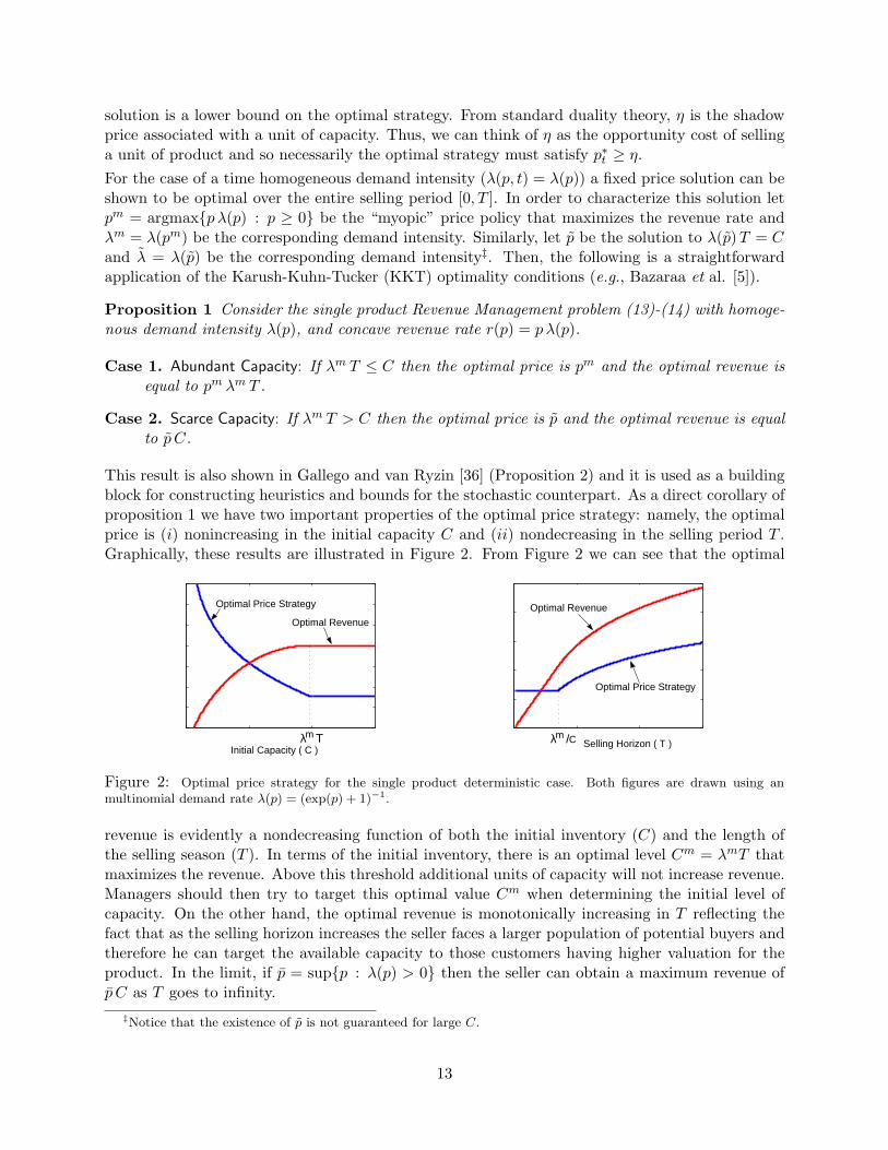
This result is also shown in Gallego and van Ryzin [36] (Proposition 2) and it is used as a buildingblock for constructing heuristics and bounds for the stochastic counterpart. As a direct corollary ofproposition 1 we have two important properties of the optimal price strategy: namely, the optimalprice is (i) nonincreasing in the initial capacity C and (ii) nondecreasing in the selling period T .Graphically, these results are illustrated in Figure 2. From Figure 2 we can see that the optimal

Initial Capacity ( C )Selling Horizon ( T )λ Τm

Optimal Price Strategy

Optimal Revenue

λ / m

Optimal Revenue

Optimal Price Strategy

C

Figure 2: Optimal price strategy for the single product deterministic case. Both figures are drawn using anmultinomial demand rate λ(p) = (exp(p) + 1)−1.

revenue is evidently a nondecreasing function of both the initial inventory (C) and the length ofthe selling season (T ). In terms of the initial inventory, there is an optimal level Cm = λmT thatmaximizes the revenue. Above this threshold additional units of capacity will not increase revenue.Managers should then try to target this optimal value Cm when determining the initial level ofcapacity. On the other hand, the optimal revenue is monotonically increasing in T reflecting thefact that as the selling horizon increases the seller faces a larger population of potential buyers andtherefore he can target the available capacity to those customers having higher valuation for theproduct. In the limit, if p = sup{p : λ(p) > 0} then the seller can obtain a maximum revenue ofp C as T goes to infinity.

‡Notice that the existence of p is not guaranteed for large C.

13

Most extensions of this single product deterministic demand problem generalize some aspect ofthe functional form of the demand process. For example, Smith and Achabal [74] studied thecase where demand intensity depends on price as well as on the level of inventory, i.e. λ(pt, Ct, t).The idea (which naturally arises in the retail sector, for instance) is that demand decreases asthe inventory is depleted. Customers are less likely to find the product they want (e.g., in termsof size, color, quality, etc.) when available inventory is low. In this setting, the authors deriveoptimality conditions for the price similar to (15), and closed form solutions are reported forthe special case of a multiplicative separable demand rate with exponential price sensitivity, i.e.,λ(p, C, t) = k(t) y(C) exp(−γp)).Another extensive stream of research coming especially from marketing (e.g., Doland and Jeuland[24]-[43], Kalish [44], Mesak and Berg [57], Mesak and Clark [58], Parker [64], among many others)considers the case of a price sensitive diffusion model (a la Bass [3]) to describe the dynamics ofthe demand. On the Revenue Management context, Feng and Gallego [28] use a diffusion modelto characterize the intensity of the demand process. The Bass diffusion model is generally used fordurable goods, for which demand at time t depends on the number of units sold previous to t andthe size of the population of potential customers. More specifically, the demand rate λ(t) at time tis a function of the current price p(t), the amount sold by that time D(t), and the population sizeN , that is,

λ(t) :=∂D(t)

∂t= λ(p(t), D(t), N). (17)

In general the diffusion effect, i.e., the dependence of the demand rate λ on the cumulative sale D(t),is not uniform over time. Upon introduction, we expect a positive effect (meaning ∂λ/∂D ≥ 0) dueto factors such as word of mouth, improved reputation, or exclusivity. On the other hand, as timepasses and the number of sold units increases, we expect market saturation and obsolescence effectsto generate a negative impact on demand (i.e., ∂λ/∂D ≤ 0). According to Kalish [44] results, theevolution of price over time can follow three generic paths: (i) monotonically increasing if word-of-mouth effects have a positive impact on demand, (ii) unimodal: increasing at the beginning,reaching a maximum at some intermediate time, and then decreasing for the rest of the sellingperiod. This situation occurs when there is a positive effect of word-of-mouth at the beginningfollowed by demand saturation. Finally, (iii) the price is monotonically decreasing over the entirehorizon if there is a negative effect of penetration on demand. For a complete review of these singleproduct Bass diffusion models we refer the reader to section §2 in Elmaghraby and Keskinocak [26].In a different context, Rajan et al. [65] and Abad [1] derive optimal pricing policies for the casewhere inventory deteriorates continuously and deterministically over time at a rate proportional tothe inventory position. The special cases of linear demand and exponential decay are studied inmore detail.

3.1.2 Multiple Product Case

The case of multiple products (|M| ≥ 2) has received considerably less attention. The reason isprobably because of the higher degree of complexity attached to these multi-product formulationsespecially to characterize demand correlation and product substitution effects. In the economicsliterature, Wilson [85] studies deterministic, multi-product models in which the seller objective itto design an optimal menu of prices and products.The selection of an appropriate consumers’ choice model such as the multinomial logit or multi-nomial probit (e.g. Ben-Akiva and Lerman [9]) to characterize customers’ preferences becomes acritical component of the problem’s formulation (e.g., Talluri and van Ryzin [79]). We notice that

14

in the case when capacity is dedicated and the price of product i does not affect the demand forproduct j 6= i (independent demands) then the multi-product case reduces trivially to a set ofdisconnected single-product problems. The interesting cases arise when capacity is flexible and/ordemand process depends on the whole vector of prices (substitute or complementary products).In general, a similar result to proposition (1) can be derived in this multi dimensional case. Forexposition purposes, we consider here the simple case of time homogenous demand processes. Inthis setting, it is not hard to show that a fixed price solution can be used without any sacrifice onperformance. Let Di(P ) = λi(P ) T be the cumulative demand for product i ∈M given a vector ofprices P = (p1, . . . , pn) (λi is the time homogenous demand rate). Let Λ(P ) = (λ1(P ), . . . , λn(P ))be the vector of demand intensities and T Λ(P )′P be the revenue function (primes (’) denote vectortranspose). In this case, it is convenient to introduce for each product i ∈ M the inverse demandfunction Pi(Λ) that represents the price of product i ∈ M given a vector of cumulative intensitiesΛ. We assume then that P (Λ) is a real valued function that is continuous and differentiable andsuch that the revenue function P (Λ)′Λ is strictly concave. The Revenue Management problem(9)-(12) can be written in this case as:

maxΛ≥0

T P (Λ)′Λ (18)

subject to T AΛ ≤ C. (19)

This is a multidimensional nonlinear programming problem which has a unique solution given theconcavity assumption on the revenue function. Similar to proposition (1), two cases characterizethe optimal solution. Let Λm be the vector of cumulative demands that maximize P (Λ)′Λ. ThenΛm is optimal if and only if T A Λm ≤ C. If this condition is not satisfied, then the optimal solutionis a boundary point Λ that satisfies the corresponding KKT optimality conditions. The followingproposition characterizes the multi-product case.

Proposition 2 Consider the multi product Revenue Management problem (18)-(19) with homoge-nous inverse demand function P (Λ), and concave revenue function T P (Λ)′ Λ.

Case 1. Abundant Capacity: If T AΛm ≤ C then the optimal price is Pm = P (Λm).

Case 2. Scarce Capacity: If T AΛm 6≤ C then let Λ be the unique solution to the following Karush-Kuhn-Tucker optimality conditions

∇Λ[P (Λ)′Λ)]−A′ β = 0β′(T AΛ− C) = 0 (20)Λ ≥ 0 β ≥ 0,

where ∇Λ is the gradient operator with respect to Λ and β is an m-dimensional vector ofLagrangian multipliers. The optimal price in this case is P = P (Λ).

Let ∂ΛP (Λ) be the Jacobian matrix associated to the price vector P (Λ). That is, the ij element ofthis matrix is given by [∂ΛP (Λ)]ij = ∂Pj(Λ)

∂λi. Thus, the first KKT condition above implies that the

optimal price vector satisfies:P (Λ) = A′β − ∂ΛP (Λ)Λ. (21)

Similar to the single product case, β is the vector of shadow prices associated with the availablecapacity C, and A′β represents the vector of opportunity cost. Therefore, additional capacity isvaluable only if it is scarce, i.e. β ≥ 0.

15

It is also important to notice that for the multi-product case it is possible that the optimal priceincreases with the level of capacity. For instance, consider a simple example with two productswhere (19) is given by two constraints: λ1 + λ2 ≤ C1 and λ1 ≤ C2. Suppose that the current levelof capacity is (C1 = 1, C2 = 0) and that the optimal solution is λ∗1 = 0, λ∗2 = 1. If we increase C2

to a new value C2 = 1, then under regular conditions on the revenue function the new solution willsatisfy λ1 > 0 and λ2 < 1. That is, an increase in C2 might induce a decrease in λ2. Thus, theoptimal price of product 2 will increase after the increase of C2. This example raises the question ofwhat the conditions are that will ensure that the optimal price is in fact nonincreasing in capacity.We partially answer this question in the following proposition based on the work by Topkis [80]and Milgrom and Roberts [59] on supermodularity and complementarity.

Proposition 3 Suppose that the inverse demand function is monotone, that is, if Λ1 ≥ Λ2 thenP (Λ1) ≤ P (Λ2). Suppose, moreover, that the objective P (Λ)′Λ is supermodular and the sets L(C) ={Λ ≥ 0 : T A Λ ≤ C} are sublattices§ . Then, the optimal solution Λ∗ to (18)-(19) is nondecreasingin C and the optimal price is nonincreasing in C.

The proof follows directly from Theorem 5 in Milgrom and Roberts [59]. The monotonicity ofP (Λ) is the extension of the classical “downward sloping demand function” condition to this multi-dimensional case. We expect the supermodularity assumption to hold when there are productsubstitution effects (such as for airline seats or hotel rooms) since in these cases the marginalreturn on product i should be increasing on the price of product j. The requirement of L(C) beinga sublattice is more restrictive. This result holds trivially when capacity is dedicated, i.e., A = Ithe identity matrix.Similarly, in the time homogenous case an increase in the selling period (i.e., T ↑) can be interpretedas a decrease in the level of capacity†. Thus, under the same set of assumptions of proposition 3,we expect the optimal price to be an increasing function of T .

3.2 Stochastic Models

Pricing policies with stochastic demand are more complex and harder to compute than their deter-ministic counterparts. For instance, in this setting a single price solution is rarely optimal unlesswe strict ourselves to this type of static policies. On the other hand, stochastic models are clearlyused more appropriately to describe real life situations where the paths of demand and inventoryare unpredictable over time and managers are forced to react dynamically by adjusting prices asuncertainty reveals itself.The natural way to tackle a problem of this type is by using stochastic dynamic programming(SDP) techniques. At every decision point during the selling season, the manager collects allrelevant information about the current inventory positions and sales and establishes the prices atwhich the products should be sold. With a few exceptions, most of the research has been done forthe single product case under Markovian assumptions on the demand process. In this setting, theinventory levels are the only relevant information that managers need to make pricing decisions.

§A function f : IRn → IR is supermodular if for all x, x′ ∈ IRn, f(x) + f(x′) ≤ f(min{x, x′}) + f(max{x, x′}. A setL ⊆ IRn is a sublattice if for all x, x′ ∈ L, min{x, x′} ∈ L and max{x, x′} ∈ L.

†Notice that in the time homogenous case the feasible region T A Λ ≤ C is equivalent to A Λ ≤ CT

.

16

3.2.1 Single Product Case

In the single product case (|M| = 1), we can assume without any loss of generality that the initialcapacity C = C0 is a scalar representing the number of units of the product that are available attime t = 0. Using an SDP formulation, we define Vt(Ct) to be the value function at time t if theinventory is Ct, that is, Vt(Ct) is the optimal expected revenue from time t to the end of the seasongiven that the current inventory position at time t is Ct. Time t has been modelled in the literatureas either a continuous or discrete variable. From a practical perspective, we expect that managerswill revise their price decisions only at discrete points in times. However, the explosive growth ofthe Internet and E-commerce make the continuous time model much more suitable for practicaluses.

Single Price Models:

The simplest approach to the problem is the single price solution. In this case, we restrict thepricing policy to be a fixed price during the entire season, i.e., pt = p for all t ∈ [0, T ]. This typeof static policy is appropriate for products having one or more of the following characteristics: (i)short selling period, (ii) high costs of changing prices, (iii) legal regulations that force the priceto be fixed. The fixed price model is simple and easy to implement and control. Hence, even ifprice changes are possible, managers often choose to use the static fixed price approach. We willsee shortly that the fixed price model is asymptotically optimal in some situations. In this singleproduct fixed price model, formulation (9)-(12) is given by

V (C, T ) = maxp≥0

V (C, p, T ) = maxp≥0

E[p min{D(p, T );C}], (22)

where D(p, T ) is the random variable representing the cumulative demand in [0, T ] at a pricep. Closed-form solutions for this problem are not available for the general case of an arbitrarydistribution of D(p, T ) but we can characterize the optimal price in terms of the demand elasticityas follows. Let f(D; p, T ) be the probability mass function of D(p, T ) (or the density function ifdemand is modelled as a continuous variable). Let also F (D; p, T ) be the probability distributionfunction of D(p, T ). We define the demand elasticity with respect to price as ε(D, p, T ) = pfp(D,p,T )

f(D,p,T )

where fp(D, p, T ) is the partial derivative of f(D, p, T ) with respect to p.

Proposition 4 The first order optimality condition for the solution of (22) is

E[min{D; C} ε(D, p, T )]E[min{D;C}] = −1. (23)

Proof: See the appendix. We note that proposition 4 extends the well-known condition in economicsthat says that the demand elasticity has to be equal to -1 at the optimal monopolistic price. Inthe stochastic case, we have that the weighted expected value of the elasticity has to be equal to-1, where the weight is given by the level of sales min{D, C}. Similar to the deterministic case, wecan show that the optimal price for this single price model is nonincreasing on the initial level ofcapacity C. We summarize this observation for the case of a continuous demand distribution† inthe next proposition. We introduce the following definition: A function g(x, y) satisfies increasingdifferences in (x, y) if g(xH , y)− g(xL, y) is nondecreasing in y for all xH ≥ xL.

Proposition 5 Suppose that F (D; p, T ) satisfies increasing differences in (D, p) and −F (D; p, T )satisfies increasing differences in (p, T ). If there is a unique optimal solution p∗(C) for (22) thenthe solution is nonincreasing in C and nondecreasing in T .

†The result and proof for the discrete case follows exactly the same line of arguments.

17

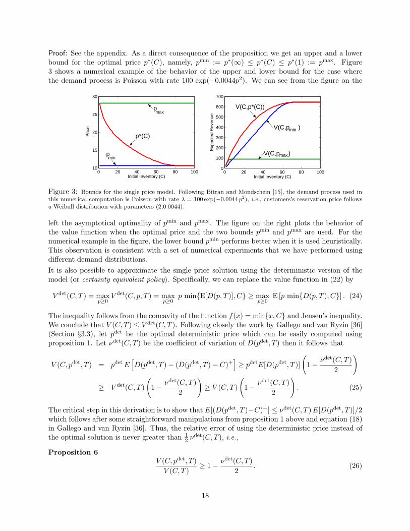
Proof: See the appendix. As a direct consequence of the proposition we get an upper and a lowerbound for the optimal price p∗(C), namely, pmin := p∗(∞) ≤ p∗(C) ≤ p∗(1) := pmax. Figure3 shows a numerical example of the behavior of the upper and lower bound for the case wherethe demand process is Poisson with rate 100 exp(−0.0044p2). We can see from the figure on the

0 20 40 60 80 10010

15

20

25

30

Initial Inventory (C)

Pric

e

0 20 40 60 80 1000

100

200

300

400

500

600

700

Initial Inventory (C)

Exp

ecte

d R

even

ue

p min

p max

p*(C)

V(C,p ) max

V(C,p ) min

V(C,p*(C))

Figure 3: Bounds for the single price model. Following Bitran and Mondschein [15], the demand process used inthis numerical computation is Poisson with rate λ = 100 exp(−0.0044 p2), i.e., customers’s reservation price followsa Weibull distribution with parameters (2,0.0044).

left the asymptotical optimality of pmin and pmax. The figure on the right plots the behavior ofthe value function when the optimal price and the two bounds pmin and pmax are used. For thenumerical example in the figure, the lower bound pmin performs better when it is used heuristically.This observation is consistent with a set of numerical experiments that we have performed usingdifferent demand distributions.It is also possible to approximate the single price solution using the deterministic version of themodel (or certainty equivalent policy). Specifically, we can replace the value function in (22) by

V det(C, T ) = maxp≥0

V det(C, p, T ) = maxp≥0

p min{E[D(p, T )], C} ≥ maxp≥0

E [p min{D(p, T ), C}] . (24)

The inequality follows from the concavity of the function f(x) = min{x,C} and Jensen’s inequality.We conclude that V (C, T ) ≤ V det(C, T ). Following closely the work by Gallego and van Ryzin [36](Section §3.3), let pdet be the optimal deterministic price which can be easily computed usingproposition 1. Let νdet(C, T ) be the coefficient of variation of D(pdet, T ) then it follows that

V (C, pdet, T ) = pdet E[D(pdet, T )− (D(pdet, T )− C)+

]≥ pdetE[D(pdet, T )]

(1− νdet(C, T )

2

)

≥ V det(C, T )

(1− νdet(C, T )

2

)≥ V (C, T )

(1− νdet(C, T )

2

). (25)

The critical step in this derivation is to show that E[(D(pdet, T )−C)+] ≤ νdet(C, T ) E[D(pdet, T )]/2which follows after some straightforward manipulations from proposition 1 above and equation (18)in Gallego and van Ryzin [36]. Thus, the relative error of using the deterministic price instead ofthe optimal solution is never greater than 1

2 νdet(C, T ), i.e.,

Proposition 6V (C, pdet, T )

V (C, T )≥ 1− νdet(C, T )

2. (26)

18

It is interesting to notice that the quality of the deterministic approximation depends on thecoefficient of variation rather than the variance itself. For instance, if the selling horizon increaseswe should expect that the variance of the cumulative demand will also increase but the coefficientof variation will probably decrease. Similarly, products having high-volume demand are more likelyto have a small coefficient of variation. Gallego and van Ryzin [37] derive a similar inequality forthe case where the demand intensity is time-varying. We will return to this point later when wediscuss the multi-period problem.The first extension of the single period model is to allow the manager to revise the price only onceduring the selling horizon. Lazear [49] considers a model of a retailer selling a single unit (C = 1)to a population (N) of potential customers whose valuation (reservation price R) for the productis unknown to the seller. The selling horizon is divided in two periods. The retailer’s problem isto set the price for the good during the first and second periods, p1 and p2 respectively. Lazear’smodel is of incomplete information. If the product does not sell in the first period at price p1, thenthe retailer can update his/her initial estimate of R to compute p2. In this stylized setting, Lazearshows that the price is monotonically decreasing with time, p1 > p2, and that the magnitude ofthe markdown p1 − p2 increases with N . This suggests that prices of high-demand goods (i.e., Nis large) adjust more rapidly to time on the market during which the good remains unsold.In a different setting, Feng and Gallego [27] study a single product two price model where the pricesin both periods are fixed and the only decision is when to switch from one to the other. Threecases are studied (i) the markdown case when p1 > p2 (e.g., the retail model), (ii) the markup casep1 < p2 (e.g., the airline model), and (iii) the general case p1 ≤ or ≥ p2. Under the assumption thatdemand at price pi is a Poisson process of intensity λi the authors derive structural properties of theoptimal stopping time problem. In particular, they show that the optimal policy is of a thresholdtype. For example, for case (i) they show that there is an increasing sequence {xn : n = 1, 2, . . .}of time thresholds such that if the inventory process is Ct then it is optimal to markdown theitems to p2 as soon as the time-to-go (T − t) is less than the time threshold xCt . Similar thresholdpolicies are derived for case (ii) and (iii). Feng and Xiao [29] extend the two price formulation inFeng and Gallego [27] to the case of a risk-sensitive seller that penalizes the variance of revenuelinearly. Other related work on the timing of sales and promotions can be found in Courty and Li[23], Krider and Weinberg [47], Warner and Barsky [82], Kinberg and Rao [46].

Dynamic Price Models:

One of the first papers that addresses the general issue of how to price a perishable productdynamically is the work by Kincaid and Darling [45]. Their setting is a continuous time modelwhere demand follows a Poisson process with fixed intensity λ. An arriving customer at timet has a reservation price rt for the product, i.e., the maximum price the customer is willing topay. From the seller perspective, the reservation price rt is a random variable with distributionF (r, t). Kincaid and Darling consider two cases. In the first case, the seller does not post pricesbut receives offers from potential incoming buyers, which he/she either accepts or rejects. It isassumed that arriving customers offer their reservation price rt, i.e, it is assumed that customersdo not act as strategic players. In the second case, the seller posts the price pt and arrivingcustomers purchase the product only if rt ≥ pt. The demand process in this situation is Poissonwith intensity λ (1−F (pt, t)). Optimality conditions for the value function Vt(Ct) and the optimalprice pt(Ct) are derived for both cases, and closed-form solutions are reported for the special caseF (r, t) = 1−exp(−r). When prices are posted, the optimality condition (Hamilton-Jacobi Bellman

19

equation) is given by

∂Vt(Ct)∂t

= maxp≥0

{λ(1− F (p, t))

[p−

(Vt(Ct)− Vt(Ct − 1)

)]}(27)

According to this condition, it is not hard to see that the optimal price satisfies pt(Ct) ≥ Vt(Ct)−Vt(Ct − 1). The difference Vt(Ct) − Vt(Ct − 1) represents the opportunity cost of selling a unitof capacity at time t when the available inventory is Ct. In the Yield Management literatureVt(Ct)−Vt(Ct− 1) is referred to as the bid price for the inventory level Ct at time t. Note that themaximization in (27) guarantees that the optimal price pt(Ct) is larger than or equal to this bidprice and therefore the value function Vt(Ct) is nondecreasing in t. Under some mild restrictionson F (p, t) and its density f(p, t)‡, the first order condition characterizes the optimal price pt(Ct)as follows:

pt(Ct) =1− F (pt(Ct), t)

f(pt(Ct), t)+ Vt(Ct)− Vt(Ct − 1). (28)

Thus, the problem of computing an optimal price strategy reduces to the computation of theopportunity cost Vt(Ct) − Vt(Ct − 1). In general, there are no exact closed-form solution for theoptimal price strategy in (27). One exception reported in Kincaid and Darling [45] is the caseof exponential reservation price distribution, that is, λ(p) = λ exp(−α p). Condition (27) is alsouseful to compute a lower bound on pt(Ct).

Proposition 7 Suppose that demand is a Poisson process with price sensitive intensity λ(1 −F (p, t)). Then, the optimal price pt(Ct) is bounded below by pmin, the solution to

pmin =1− F (pmin, t)

f(pmin, t). (29)

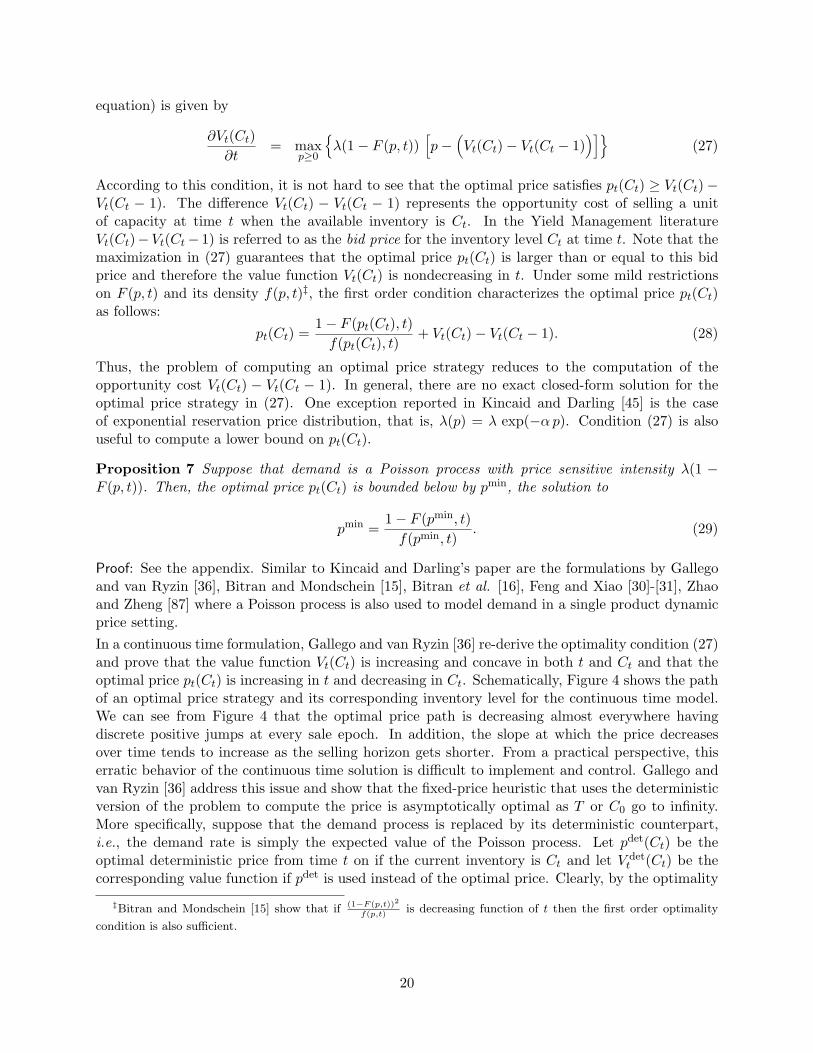
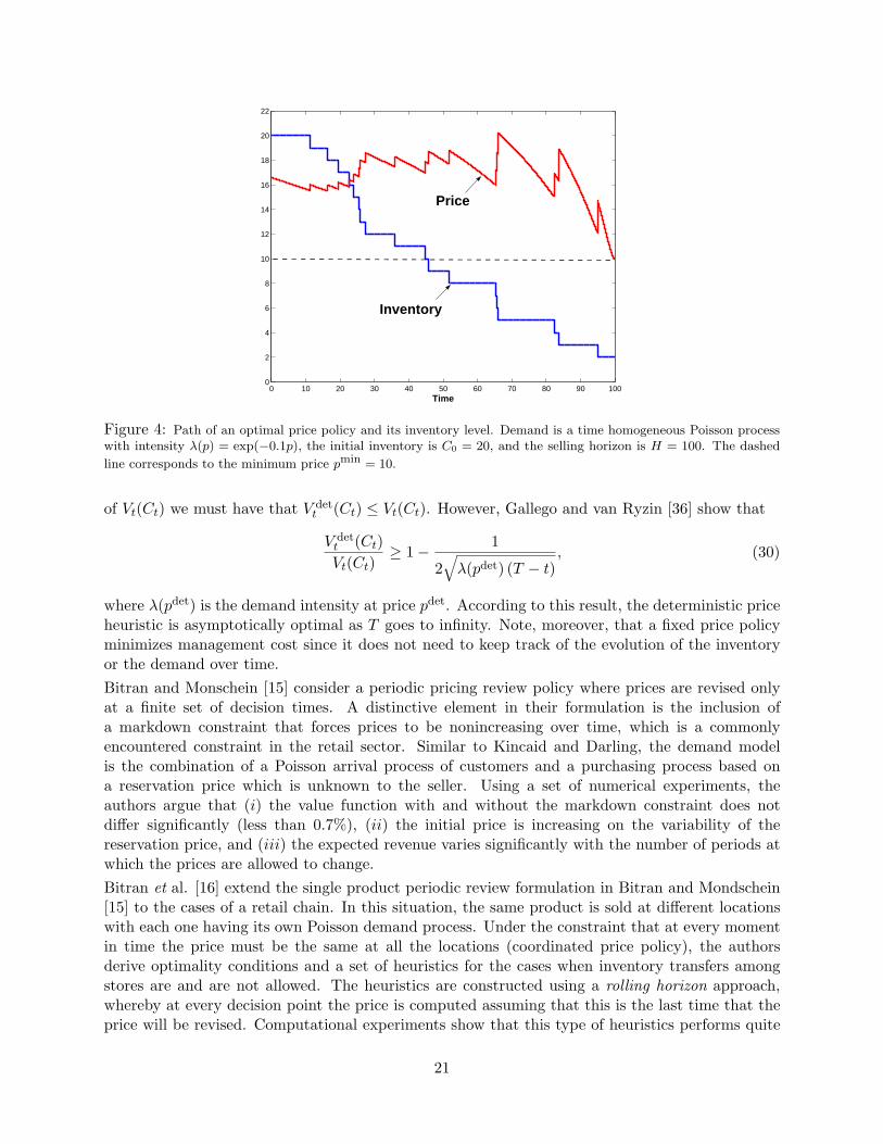
Proof: See the appendix. Similar to Kincaid and Darling’s paper are the formulations by Gallegoand van Ryzin [36], Bitran and Mondschein [15], Bitran et al. [16], Feng and Xiao [30]-[31], Zhaoand Zheng [87] where a Poisson process is also used to model demand in a single product dynamicprice setting.In a continuous time formulation, Gallego and van Ryzin [36] re-derive the optimality condition (27)and prove that the value function Vt(Ct) is increasing and concave in both t and Ct and that theoptimal price pt(Ct) is increasing in t and decreasing in Ct. Schematically, Figure 4 shows the pathof an optimal price strategy and its corresponding inventory level for the continuous time model.We can see from Figure 4 that the optimal price path is decreasing almost everywhere havingdiscrete positive jumps at every sale epoch. In addition, the slope at which the price decreasesover time tends to increase as the selling horizon gets shorter. From a practical perspective, thiserratic behavior of the continuous time solution is difficult to implement and control. Gallego andvan Ryzin [36] address this issue and show that the fixed-price heuristic that uses the deterministicversion of the problem to compute the price is asymptotically optimal as T or C0 go to infinity.More specifically, suppose that the demand process is replaced by its deterministic counterpart,i.e., the demand rate is simply the expected value of the Poisson process. Let pdet(Ct) be theoptimal deterministic price from time t on if the current inventory is Ct and let V det

t (Ct) be thecorresponding value function if pdet is used instead of the optimal price. Clearly, by the optimality

‡Bitran and Mondschein [15] show that if (1−F (p,t))2

f(p,t)is decreasing function of t then the first order optimality

condition is also sufficient.

20

0 10 20 30 40 50 60 70 80 90 1000

2

4

6

8

10

12

14

16

18

20

22

Time

Inventory

Price

Figure 4: Path of an optimal price policy and its inventory level. Demand is a time homogeneous Poisson processwith intensity λ(p) = exp(−0.1p), the initial inventory is C0 = 20, and the selling horizon is H = 100. The dashed

line corresponds to the minimum price pmin = 10.

of Vt(Ct) we must have that V dett (Ct) ≤ Vt(Ct). However, Gallego and van Ryzin [36] show that

V dett (Ct)Vt(Ct)

≥ 1− 1

2√

λ(pdet) (T − t), (30)

where λ(pdet) is the demand intensity at price pdet. According to this result, the deterministic priceheuristic is asymptotically optimal as T goes to infinity. Note, moreover, that a fixed price policyminimizes management cost since it does not need to keep track of the evolution of the inventoryor the demand over time.Bitran and Monschein [15] consider a periodic pricing review policy where prices are revised onlyat a finite set of decision times. A distinctive element in their formulation is the inclusion ofa markdown constraint that forces prices to be nonincreasing over time, which is a commonlyencountered constraint in the retail sector. Similar to Kincaid and Darling, the demand modelis the combination of a Poisson arrival process of customers and a purchasing process based ona reservation price which is unknown to the seller. Using a set of numerical experiments, theauthors argue that (i) the value function with and without the markdown constraint does notdiffer significantly (less than 0.7%), (ii) the initial price is increasing on the variability of thereservation price, and (iii) the expected revenue varies significantly with the number of periods atwhich the prices are allowed to change.Bitran et al. [16] extend the single product periodic review formulation in Bitran and Mondschein[15] to the cases of a retail chain. In this situation, the same product is sold at different locationswith each one having its own Poisson demand process. Under the constraint that at every momentin time the price must be the same at all the locations (coordinated price policy), the authorsderive optimality conditions and a set of heuristics for the cases when inventory transfers amongstores are and are not allowed. The heuristics are constructed using a rolling horizon approach,whereby at every decision point the price is computed assuming that this is the last time that theprice will be revised. Computational experiments show that this type of heuristics performs quite

21

well with an average error of 2%-3%. The paper also includes a set of numerical experiments thatwere conducted using real data collected from a retail chain store.Zhao and Zheng [87] study the single product pricing problem for the case where the arrival processof customers is a time dependent Poisson process. They also use a reservation price formulationsimilar to Kincaid and Darling [45] or Bitran and Mondschein [15] to model the purchasing decisionsof the customers. For this problem, Zhao and Zheng derive optimality condition equivalent to (27)and show that the value function is concave on both the level of inventory and the duration of theselling season. They also prove that the optimal price is nonincreasing in the level of inventory andfind a sufficient condition on the reservation price distribution that guarantees that the optimalprice is nondecreasing for the duration of the selling horizon.Another variation to the basic single-product Poisson demand problem that has received someattention is the case where there is a finite set of predetermined prices {p1, . . . , pk} from which theseller can choose. Gallego and van Ryzin [36] discuss this issue and show that the deterministicsolution, which involved using at most two different prices from the list, is again asymptoticallyoptimal as the initial capacity and selling horizon increase. Independently, Chatwin [20] and Fengand Xiao [31] provide a systematic analysis of the pricing policy and value function for the problemwith a finite set of prices. In these papers it is shown that the value function is concave on boththe initial inventory and duration of the selling horizon and that the optimal price is nonincreasingin the inventory and decreasing in the time remaining. An upper bound on the maximum numbersof price changes is also reported. In addition, Feng and Xiao [31] show that there is a maximalsubset P0 ⊆ {p1, . . . , pk} such that the revenue rate is increasing and concave within P0 and theoptimal price at any time belongs necessarily to P0. This observation is particularly useful sinceit narrows down the set of potential optimal prices making the computation of the optimal pricingstrategy much easier. Feng and Xiao [30] impose the additional constraint that prices have tochange monotonically and both the markdown and markup cases are considered.The stochastic version of Kalish [44] is studied by Raman and Chatterjee [67]. Specifically, theauthors consider a discounted infinite horizon problem where cumulative demand D(t) follows astochastic differential equation

dD(t) = f(D(t), p(t)) dt + σ(D(t)) dw(t). (31)

f(D, p) is a deterministic function of cumulative sales and price and w(t) is a Wiener process. Forthis formulation, Raman and Chatterjee derive the Hamilton-Jacobi-Bellman optimality equationand show that for the linear demand case, f(D, p) = a − bp, the optimal price strategy is linearlydecreasing in D and monotonically increasing in the demand uncertainty (σ). Similar results arederived for two alternative demand formulations: the multiplicatively separable demand functionand the simple price-timing model.Inspired by the results in Gallego and van Ryzin [36] related to the deterministic fixed-price heuris-tic, we conclude this single product section extending their results to the discrete time formulation.Specifically, we consider the case of a periodic review model with N periods. In each periodn = 1, . . . , N a fixed price pn is charged and Dn(pn) is the corresponding (random) demand. Let{pdet

n : n = 1, . . . , N} be the optimal deterministic solution, i.e, the solution to the followingproblem.

V det1 (C0) = max

p1,...,pN

N∑

n=1

pn E[Dn(pn)] (32)

22

subject toN∑

n=1

E[Dn(pn)] ≤ C0. (33)

In order to ensure feasibility, we assume that there is a price p∞ such that∑N

n=1 E[Dn(p∞)] < C0.The following result provides an estimate of the quality of the deterministic solution. We defineDdet

n :=∑n

i=1 Dn(pdet) to be the cumulative demand up to period n and σ2n to be the variance of

Ddetn . We also define ηdet

n (C0) as follows.

ηdetn (C0) :=

√σ2

n + (C0 − E[Ddetn ])2 − (C0 − E[Ddet

n ])

2. (34)

Proposition 8 Suppose that the deterministic problem (32)-(33) is feasible with concave objectiveand convex feasible region. Then, the optimal expected revenue V1(C0) is bounded above by thedeterministic solution, that is, V1(C0) ≤ V det

1 (C0). In addition, let V1(pdet, C0) be the expectedrevenue that is obtained using the deterministic prices {pdet

n : n = 1, . . . , N}.Then, we have that

1 ≥ V1(pdet, C0)V1(C0)

≥ 1V det

1 (C0)

N∑

n=1

pdetn E[Dn(pdet

n )]

(1− ηdet

n (C0)E[Dn(pdet

n )]

)≥ 1−max

n

ηdetn (C0)

E[Dn(pdetn )]

.

(35)Finally, in the time homogeneous case E[Dn(p)] = Tn λ(p), where λ(p) is time invariant demandintensity and Tn is the duration of period n, a single price pdet solves (32)-(33) and

1 ≥ V1(pdet, C0)V1(C0)

≥ 1− ν(C0)2

, (36)

where ν(C0) is coefficient of variation of DdetN the cumulative demand over the entire selling horizon.

Proof: See the appendix. We note that if there is no uncertainty on the demand, then the boundsare tied. Proposition 8 shows that it is the coefficient of variation of the demand and not thevariance that regulates the quality of the deterministic price heuristic. For instance, consider thetime homogeneous case where E[Dn(pdet)] = Tn λ(pdet) and Var(Dn(pdet)) = Tn σ2(pdet)§. In thiscase, the results in proposition 8 imply that

1 ≥ V1(pdet, C0)V1(C0)

≥ 1− νdet

2√

Twhere νdet =

σ(pdet)λ(pdet)

and T =N∑

n=1

Tn. (37)

This result says that the relative error of the deterministic solution is proportional to the inverseof the square root of the selling horizon T . A similar result is reported by Gallego and van Ryzin[36] for the case of a Poisson process.

3.2.2 Multiple Product Case

Similar to the deterministic case, the research on optimal pricing policy in a multiple product settingis narrower in scope than the single product counterpart. There is an important case, however,that has received considerable attention especially in the Yield Management literature on airlineseat control. The setting is that of a single resource that is used to satisfy a set of different demand

§Stochastic processes like the Poisson process or the Brownian motion with stationary and independent incrementssatisfy these assumptions.

23

classes. The example of airline seats is of course one where companies use the same resource toaccommodate leisure and business travellers. Other applications are in the management of hotelrooms or bandwidth capacity of an Internet provider. In order to price the same units of capacitydifferently, companies need to identify characteristics that differentiate their potential customersand classify them accordingly. For example, airlines differentiate leisure passengers from businesspassengers according to their willingness to stay a Saturday night at their destinations.

Static Price Models:

Much of the research on this problem takes a static view of the price. Specifically, prices or fares forthe different classes are predetermined and the seller’s problem is to accept or reject the incomingrequests of customers dynamically as functions of time, unsold capacity, and the type (fare). Wecan still, however, view this problem as a dynamic pricing problem. In fact, for each class j theseller has two possible prices to set at each moment of time. One is the fixed and predefined pricepj and the other is a high price pnull

j À pj , the null price, for which class-j demand at that priceis almost surely zero. The null price can be thought of as an artificial way to model customers’rejections in the context of pricing policies.For the sake of space, we do not provide here an exhaustive review of the literature that hasaddressed this problem. Readers are referred to the survey papers by Belobaba [7] and McGill andvan Ryzin [56] for a more systematic review of the inventory (seat) control literature.The general multiple product version of this problem can be stated as follows.

1. Data: An initial m-dimensional vector of resource C0, a menu of product M having fixedand predetermined prices pj (j = 1, . . . ,M), and a consumption matrix A = [aij ] such thataij is the amount of resource i consumed by one unit of product j.

2. Problem: Find an admission/rejection policy u(t, Ct, j) ∈ {0, 1} such that if the currentinventory at time t is Ct and there is a customer demanding product j then u = 1 if the orderis accepted and u = 0 if the order is rejected.

In our pricing setting, given an inventory Ct at time t we can redefine step 2 as follows: charge pricepj for product j if u(t, Ct, j) = 1 otherwise charge price pnull

j . The equivalence between rejectionsand null prices implicitly assumes that the effects on the demand process of rejecting customers orcharging the null prices are the same.As we already mentioned, much of the results on this problem have been obtained for the singleresource (or single leg) case using (i) a continuous time formulation with Poisson demand processes(e.g. Liang [51], Zhao and Zheng [88], Feng and Xiao [32]-[33]), or (ii) a discrete time modelwith arbitrary demand but with the restriction that at most one customer can arrive per period(e.g., Lee and Hersh [50], Subramanian et al. [76]). Let Vt(C) be the optimal value function attime t if the current inventory is C and let βt(C) = Vt(C) − Vt(C − 1) be the corresponding bidprice function. Then, it is optimal to sell a unit of product j at time t if and only if pj ≥ βt(C)in the continuous time case or if pj ≥ βt−1(C) in the discrete time version. Otherwise, the nullprice pnull

j (i.e., rejection) is recommended. If we assume that for all j pnullj > βt(C) for all t

and C, then the optimal pricing policy for class j at time t, given an inventory C, is to set theminimum price p ∈ {pj , p

nullj } such that p ≥ βt(C). This property of the optimal solution, which

follows directly from the Bellman equation, emphasizes the importance of the opportunity cost ofcapacity described by the bid prices. Not surprisingly, then, much of the research has focused oncharacterizing the main properties of βt(C) such as its monotonicity, i.e., nonincreasing in both tand C. In this single resource case, these properties imply a nested structure of the optimal policy.

24

That is, if it is optimal at time t to accept class j with price pj then it is optimal to accept anyclass k with pk ≥ pj .The multi resource problem (or network Revenue Management) does not differ much from thesingle resource case in terms of optimality condition. The main difference is that bid prices inthis case are dependent on the class of the demand. More specifically, if at time t the currentvector of capacity is C and there is a request for product j and if we accept the offer we collecta price pj and inventory decreases to a new level C − A·j , where A·j is the jth column of theconsumption matrix A, i.e., the amount of resources used by product j. Thus, if Vt(C) is the valuefunction at time t when the inventory is C then it would be optimal to accept a product j requestif pj ≥ Vt(C)− Vt(C − A·j) := βt(C, j). Network Revenue Management models have been studiedby Glover et al. [40], Talluri and van Ryzin [77]-[78], You [86], de Boer et al. [17], Gunther et al.[41], Bertsimas and Popescu [10], Feng and Lin [34], Cooper [22]. In general, in these papers† theseller does not control prices but he/she is only able to accept or reject incoming orders based ontheir type and the bid prices βt(C, j).The problem of computing, or estimating, bid prices has been addressed from different angles. Thefirst, and probably most straightforward, approach is to use a deterministic formulation to estimatethe value function. In particular, if the prices for the different products {pj} are fixed, then thestatic deterministic version of our Revenue Management problem (9)-(12) is given by

V dett (C) = max

x

∑

j

pjxj (38)

Subject to Ax ≤ C (39)0 ≤ x ≤ E[D(t, T )], (40)

where E[D(t, T )] is the expected cumulative demand vector from t to the end of the horizon inT . Williamson [84] was one of the first to compute bid prices using the deterministic network flowformulation above. In particular, the dual variables associated with constraint (39) represent themarginal change in V det

t (C) as a function of the RHS vector C. Thus, if we call δ the vector ofdual variables, it is possible to approximate βt(C, j) = Vt(C) − Vt(C − A·j) by δ′A·j . Regardingthe quality of this approximation, we can first note that δ captures only the marginal change ofV det

t (C) with respect to C, that is, δ = ∇V dett (C). Thus, if the solution to (38)-(40) is sensitive to

the values of C then we should expect δ′A·j to be a bad approximation for βt(C, j). This problem,however, can be easily corrected by computing directly the difference V det

t (C) − V dett (C − A·j)

solving two times the deterministic problem (38)-(40) for the levels C and C −A·j of the capacity(e.g., Bertsimas and Popescu [10]). In addition to this, the deterministic solution relies only onthe expected value of the demand. This is clearly another source of error especially when demandvariability is high. Talluri and van Ryzin [78] use a randomized version of (38)-(40) to solve thisproblem. Specifically, they propose to estimate the value of δ simulating N independent valuesof D(t, T ), for each value they compute the corresponding dual vector and finally estimate δ asthe average of the different dual vectors obtained from the simulations (a Monte Carlo simulationapproach is also proposed in Bertsimas and Popescu [10]).

Dynamic Price Models:

Dynamic pricing models for network Revenue Management have been studied by Gallego and vanRyzin [37]. Using a Poisson demand formulation, the authors derive the HJB equation similar to

†One exception is the paper by Gallego and van Ryzin [37].

25

(27). For this multiple product case, the optimality condition is given by

∂Vt(Ct)∂t

= supp

n∑

j=1

λj(p) [pj − (Vt(Ct)− Vt(Ct −A·j))]

, (41)

where λj(p) is the demand intensity for product j for a vector of prices p. Closed-form solutionsfor this differential equation are rarely available. For this reason, Gallego and van Ryzin study twoheuristics based on the deterministic solution. Suppose that pdet(t) and λdet(t) are the optimalprice path and demand intensity, respectively, for the deterministic version of the problem, i.e.,the problem that results from replacing the stochastic demand by its expected value. The value ofpdet(t) can be obtained using the results in section §3.1.2. The first heuristic, Make-to-Stock policy,computes the expected number of orders for product j, say zj , under the deterministic solution.That is,

zj =⌊ ∫ T

0λdet

j (t) dt⌋

(42)

and it preassembles in advance exactly zj units of product j at the beginning of the selling period.The price of the products is set to be the deterministic solution pdet(t). In this Make-to-Stockheuristic, once the zj units of product are built there is no future rearrangement of capacity. Thesecond heuristic, Make-to-Order policy, also follows the deterministic price path, pdet(t), but itdoes not assemble any product in advance. Rather, this policy waits for orders to arrive andbuilds products as they are requested. Gallego and van Ryzin show that these two heuristics areasymptotically optimal as the expected sales volume goes to infinity. They also extend their modelto include overbooking and no-shows.

4 Summary of Results and New Directions

In terms of results, much of the research on dynamic pricing has focused on the problem faced by amonopolist selling a single product and having perfect information about the demand distribution.The deterministic solution of this problem, where demand is replaced by its expected value, can beobtained using standard optimization techniques (section §3.1) and represents a good approximationfor the more complicate stochastic version (proposition 8), especially for high-volume demandproducts having long selling horizons. On the other hand, the exact analysis of the stochastic caseand its optimal pricing strategy requires the solution of the Hamilton-Jacobi-Bellman equation(27). This is in general a complex differential equation for which closed form solutions are rarelyavailable; one exception is the case of exponential demand intensity (see Kincaid and Darling [45]).From the HJB equation, the difference Vt(Ct)− Vt(Ct − 1), which represents the opportunity costof selling one unit of product at time t when the available inventory is Ct, is the key componentthat has to be computed in order to determine the optimal pricing policy. Not surprisingly, theapproximation of this opportunity cost has been the departing point for many approximations andheuristics like the well-known EMSR method proposed by Belobaba [6] for airline seat control.Static single price formulations, like those presented in section §3.2.1, are also sources of goodapproximations specially when they are used on a rolling-horizon basis (e.g., Bitran et al. [16]).The multiple product dynamic pricing problem has received considerably less attention. Much ofthe research on this subject has assumed a static view of prices, where the main decision is whetherto accept or reject a given customer’s request as a function of time, available inventory, and thecorresponding fixed price attached to the incoming order. Again, the deterministic version of the

26

problem (certainty equivalent control) has been the starting point for most approximations. Gallegoand van Ryzin [37] show that two heuristics based on the deterministic solution are asymptoticallyoptimal as the volume of sales increases. In this multiple product case, the opportunity cost ofselling a unit of product j at time t is given by Vt(Ct) − Vt(Ct − A·j). Approximations for thisquantity form the basis of the so called bid price control methods. These bid prices are generallycomputed at the resource level and they represent the opportunity cost of selling one unit of aresource. Using a deterministic formulation like (38)-(40), bid prices can be interpreted as theshadow prices for the capacity constraint. The connection between bid prices and opportunitycosts is studied in Talluri and van Ryzin [77]. In this paper, using a simple example, the authorsshow that, while bid price policies are generally suboptimal, they are asymptotically optimal ascapacity increases (see also Cooper [22]).As we compare our generic formulation in (9)-(12) with the results presented in section §3 a numberof research opportunities become evident. First of all, from the demand side there are at least twoimportant considerations: (i) demand learning and (ii) demand substitution effects. In general, theresearch that we have presented in this paper assumes that the demand probability distribution isperfectly known to the seller at the beginning of the selling horizon. In practice, this is hardly thecase especially for new products for which there are no historical sales data. It would be interestingto extend the dynamic pricing models to capture demand learning as the selling process evolves,for instance using Bayesian updating. In this case, the pricing strategy can be used to control notonly revenues but also the speed at which the seller learns about customers’ preferences.On the demand substitution side, we believe there is an opportunity to combine the ongoing effortsin marketing research to understand consumer choice behavior (e.g., Roberts and Lillien [68])with the modeling and solution techniques that we have presented in this review. In general, theRevenue Management literature has tangentially discussed this connection. Talluri and van Ryzin[79] analyze the yield management problem of capacity control under a generic customer choicemodel. However, the issue of setting a dynamic pricing strategy for a given choice model remainsopen. Some results have been obtained using the traditional multinomial logit model.Closely related to the issue of demand substitution is the problem of product design and bundling.As we briefly mentioned in section §2, the seller owns an initial vector of capacity C0 that he canuse to produce a set of final products. All the research that we have discussed assumes that theset of products is exogenously given. However, in practice the seller has the ability to decide whichspecific configurations will be available to customers. The optimal decision of which products tooffer is strongly connected to the pricing strategy.The problem of computing an optimal pricing strategy for the multiple product case with periodicprice reviews is technically challenging and certainly of practical importance. In this setting,and because of product substitution effects, the whole path of the demand is needed to computerevenues. This technicality makes the solution of the HJB equation particularly hard. In this area,Awad et al. [2] have obtained some preliminary results using approximate dynamic programming.Incorporating rationality on the behavior of customers is another interesting field of research. Forinstance, how should the seller set the prices if customers act strategically. The natural way totackle this problem is using a game theoretical approach. For example, Besanko and Winston [11]solve the problem of a seller having unlimited capacity that sets the price of the product during Tdiscrete time periods. In every period each consumer, who has not yet bought the product, decideswhether of not to make a purchase at the price posted by the seller. Besanko and Winston solve forthe subgame perfect Nash equilibria. A different setting occurs when the seller prefers to conduct anauction to sell the units. Depending on the nature of the initial capacity and the menu of products

27

offered by the seller the auction might be simple or combinatorial. Vulcano et al. [81] investigatethe case of a seller having k units to auction during T discrete time periods. Every period a randomnumber of consumers show-up at the auction and are assumed to be independent, in terms of theirvaluation, of all other customers in the game. Thus, dynamic strategies from the customers’ sideare not captured by their model. Based on the revenue equivalent theorem the authors formulate adynamic programming model that solves the problem. We believe that incorporating the strategicbehavior of consumers –extending the models by Besanko and Winston or Vulcano et al.– is animportant topic especially for Internet based applications. The Internet offers customers the abilityto keep track of the evolution of the selling process and therefore to modify their buying behavioraccordingly. In addition, auction mechanisms are particularly suitable for the Internet.Including market competition is another important extension to the model. For instance, a seniorexecutive of a mayor retailer chain in Latin America recognizes that price competition amongretailers is today the main driver in their selection of a particular pricing policy.Finally, we conclude this list of potential new directions pointing at the seller’s risk neutrality.Essentially all the models that we have discussed assume that the seller is risk neutral. Feng andXiao [29] is one of the exceptions. However, most product managers in charge of these dynamicpricing policies present some degree of risk aversion. It would be interesting to measure the impactof adding risk aversion to the Revenue Management formulation. Presumably, the quality of thedeterministic solution should be even better.

AcknowledgmentsThe authors thank Victor Araman and three anonymous referees for helpful suggestions.

References

[1] Abad, P.L. 1996. Optimal Pricing and Lot-Sizing under Conditions of Perishability and PartialBackodering. Mgmnt. Sci. 42, 1093-1104.

[2] Awad, P., G. Bitran, S. Mondschein. 2000. Pricing Policies for a Family of Substitute Perish-able Products. Working paper, MIT Sloan School of Management.

[3] Bass, F.M. 1969. A New Product Growth Model for Consumer Durables. Mgmnt. Sci. 15,53-72.

[4] —. 1980. The Relationship Between Difussion Rates, Experience Curves, and Demand Elas-ticities for Consumer Durable Technological Innovations. J. of Business 53, S51-S67.

[5] Bazaraa, M.S., H.D Sherali, C.M. Shetty. 1993. Nonlinear Programming: Theory and Algo-rithms. John Wiley & Sons, Inc.

[6] Belobaba, P. 1987. Air Travel Demand and Airline Seat Inventory Management. Ph.D. Dis-sertation, MIT.

[7] —. 1987. Airline Yield Management: An Overview of Seat Inventory Control. Trans. Sci. 21,63-73.

[8] —. 1989. Application of a Probabilistic Decision Model to Airline Seat Inventory Control.Ops. Res. 37, 183-197.

[9] Ben-Akiva, M., S.R. Lerman. 1985. Discrete Choice Analysis: Theory and Application toTravel Demand. The MIT Press, Cambridge, Massachusetts.

28

[10] Bertsimas, D., I. Popescu. 2000. Revenue Management in a Dynamic Network Environment.Forthcoming in Transportation Science.

[11] Besanko, D., W. Wynston. 1990. Optimal Pricing Skimming by a Monopolist Facing RationalConsumers. Mgmnt. Sci. 36, 555-567.

[12] Bitran, G., S Mondschein. 1995. An Application of Yield Management to the Hotel IndustryConsidering Multiple Stays. Ops. Res. 43, 427-443.

[13] —,—. 1996. Mailing Decisions in the Catalog Sales Industry. Management Science 42.

[14] —, S.M. Gilbert. 1996. Managing Hotel Reservations with Uncertain Arrivals. Ops. Res. 44,35-49.

[15] —, S. Monschein. 1997. Periodic Pricing of Seasonal Product in Retailing. Mgmnt. Sci. 43,427-443.

[16] —, R. Caldentey, S. Mondschein. 1998. Coordinating Clearance Markdown Sales of SeasonalProducts in the Retail Chains. Ops. Res. 46, 609-624.

[17] de Boer, S.V., R. Freling, N. Piersma. 2002. Methematical Programming for Network RevenueManagement Revisited. Eur. J. Ops. Res. 137, 72-92.

[18] Brynjolfsson, E., Smith M. (1999). Frictionless Commerce? A Comparison of Internet andConventional Retailers. Mgmnt. Sci. 46, No. 4, 563-585.

[19] Carol, W.J., R.C. Grimes. 1995. Evolutionary Change in Product Management: Experiencesin the Car Rental Industry. Interfaces 25, 84-104.

[20] Chatwin, R.E. 2000. Optimal Dynamic Pricing of Perishable Products with Stochastic De-mand and a Finite Set of Prices. Eur. J. Op. Res. 125, 149-174.

[21] Ciancimino, A., G. Inzerillo, S. Lucidi, L. Palagi. 1999. A Mathematical Programming Ap-proach for the Solution of the Railway Yield Management Problem. Trans. Sci. 33, 168-181.

[22] Cooper, W.L. 2002. Asymptotic Behavior of an Allocation Policy for Revenue Management.Ops. Res. 50, 720-727.

[23] Courty, P., H. Li. 1999. Timing of Seasonal Sales. Journal of Business. 72, 545-572.

[24] Doland, R.J., A.P. Jeuland. 1981. Experience Curves and Dynamic Demand Models: Impli-cations for Optimal Pricing Strategies. J. Marketing 45, 52-62.

[25] Eliashberg, J., A.P. Jeuland. 1986. The Impact of Competitive Entry in a Developing MarketUpon Dynamic Pricing Strategies. Marketing Sci. 5, 20-36.

[26] Elmaghraby, W., P. Keskinocak. 2002. Dynamic Pricing: Research Overview, Current Prac-tices and Future Directions. Working paper, Georgia Institute of Technology.

[27] Feng, Y., G. Gallego. 1995. Optimal Starting Times for End-of-Season Sales and OptimalStopping Times for Promotional Fares. Mgmnt. Sci. 41, 1371-1391.

[28] —,—. 2000. Perishable Asset Revenue Management with Markovian Time Dependent De-mand Intensities. Mgmnt. Sci. 46, 941956.

29

[29] —, B. Xiao. 1999. Maximizing Revenues of Perishable Assets with a Risk Factor. Ops. Res.47, 337-341.

[30] —, —. 2000. Optimal Policies of Yield Management with Multiple Predetermined Prices.Mgmnt. Sci. 48, 332-343.

[31] —,—. 2000. A Continuous-Time Yield Management Model with Multiple Prices and Re-versible Price Changes. Mgmnt. Sci. 48, 644-657.

[32] —.—. 2001. A dynamic Airline Seat Control Model and Its Optimal Policy. Ops. Res. 49,938-949.

[33] —,—.2002. Intergration of Price and Seat Inventory Control for Airline Revenue Management.Working paper.

[34] —, P. Ling. 2002. Optimal Booking Control on a Two-Leg Flight with Multiple Fares. Workingpaper.

[35] Fisher M., A. Raman. 1996. Reducing the Cost of Demand Uncertainty Through AccurateResponse to Early Sales. Ops. Res. 44, 87-99.

[36] Gallego, G., G. van Ryzin G. 1994. Optimal Dynamic Pricing of inventories with StochasticDemand over Finite Horizons. Mgmnt. Sci. 40, 999-1020.

[37] —,—. 1997. A Multiproduct Dynamic Pricing Problem and Its Applications to Network YieldManagement. Ops. Res. 45, 24-41.

[38] Gelfand, I.M., Fomin S.V. (1963). Calculus of Variations. Prentice-Hall, Inc.

[39] Geraghty, M.K., E. Johnson. 1997. Revenue Management Saves National Car Rental. Inter-faces 27, 107-127.

[40] Glover, F. R. Glover, J. Lorenzo, C. McMillan. 1982. The Passenger-Mix Problem in theScheduled Airlines. Interfaces, 12, 73-79.

[41] Gunther, D.P., V.C.P. Chen, E.L. Johnson. 1999. Airline Yield Management: Optimal BidPrices for Single-Hub Problems Without Cancellations. Working paper.

[42] Jain, D.C., R.C. Rao. 1990. Effect of Price on the Demand for Durables: Modeling, Estima-tion, and Findings. J. of Business and Economic Statistics 8, 163-170.

[43] Jeuland A.P., R.J. Dolan. 1982. An Aspect of New Product Planning: Dynamic Pricing. InA. Zoltners (Ed.), TIMS Studies in the Management Science, Special Issue on MarketingPlanning Models, 1-21.

[44] Kalish, S. 1983. Monopolist Pricing and Dynamic Demand and Production Cost. MarketingSci. 2, 135-159.

[45] Kincaid, W.M., D.A. Darling. 1963. An inventory Pricing Problem. J. Math. Analysis App.7, 183-208.

[46] Kinberg, Y., A.G. Rao. 1975. Stochastic Models of a Price Promotion. Mgmnt. Sci. 21, 897-907.

30

[47] Krider, R., C. Weinberg. 1998. Competitive Dynamics and the Introduction of new Products:The Motion Picture Timing Game. J. Marketing Res. 35, 1-15.

[48] Ladany, S., A. Arbel. 1991. Optimal Cruise-Liner Passenger Cabin Pricing Policy. Eur. J.Ops. res. 55 136-147.

[49] Lazear, E.P. 1986. Retail Pricing and Clearance Sales. Amer. Econo. Rev. 76, 14-32.

[50] Lee, T.C., M. Hersh. 1993. A Model for Dynamic Airline Seat Inventory Control with MultipleSeat Bookings. Trans. Sci. 27, 252-265.

[51] Liang, Y. 1999. Solution to the Continuous Time Dynamic Yield Management Model. Trans.Sci. 33, 117-123.

[52] Littlewood, K. 1972. Forecasting and Control of Passenger Bookings. AGIFORS 12th AnnualSymposium Proceedings, 95-128.

[53] Mantrala M.K., S. Rao. 2001. A Decision-Support System that Helps Retailers Decide OrderQuantities and Markdowns for Fashion Goods. Interfaces 31, S146-S165 Part 2.

[54] Mas-Colell, A., D. Whinston , and J. Green . 1995. Microeconomic Theory. Oxford UniversityPress.

[55] Kurawarwala, A., H. Matsuo. 1996. Forescating and Inventory Management of Short Life-Cycle Products. Ops. Res. 44, 131-150.

[56] McGill, J.I., G.J. van Ryzin. 1999. Revenue Management: Research Overview and Prospects.Trans. Sci. 33, 233-256.

[57] Mesak, H.I., W.D. Berg. 1995. Incorporating Price and Replacement Purchases in New Prod-uct Diffusion Models for Consumer Durables. Decision Sci. 4, 425-449.

[58] Mesak H.I., J.W. Clark. 1998. Monopolist Optimum Pricing and Advertising Policies forDiffusion Models of New Product Innovations. Opt. Cont. Appl. Meth. 19, 111-136.

[59] Milgrom, P., J. Roberts. 1990. The Economics of Modern Manufacturing: Technology. Strat-egy, and Organization. Amer. Econ. Rev. 80, 511-528.

[60] Miller, B.L. 1968. Finite State Continuous Time Markov Decision Processes with a FinitePlanning Horizon. SIAM J. Control 6, 266-280.

[61] Nagle, T. 1984. Economic Foundations for Pricing. J. Business 57, S3-S26.

[62] Nair, S.K., R. Bapna. 2001. An Application of Yield Management for Internet ServiceProviders. Naval Res. Log. 48, 348-362.

[63] Oren, S.S., S.A. Smith. 1993. Service Opportunities for Electric Utilities: Creating DifferentialProducts. Kluwer Acad. Pub., Boston.

[64] Parker, P.M. 1992. Price Elasticity Dynamic Over the Adoption Life Cycle. Marketing Res.XXIX, 358-367.

[65] Rajan, A., Rakesh, R. Steinberg. 1992. Dynamic Pricing and Ordering Decisions by a Mo-nopolist. Mgmnt. Sci. 38, 240-262.

31

[66] Raman, A., N. DeHoratius, Z. Ton. 2001. Execution: The Missing Link in Retail Operations.California Management Review 43, 136-152.

[67] Raman, K., R. Chatterjee. 1995. Optimal Monopolist Pricing Under Demand Uncertainty inDynamic Markets. Mgmnt. Sci. 41, 144-162.

[68] Roberts, J., G. Lillien. 1993. Explanatory and Predictive Models of Consumer Behavior.Chapter 2 in Handbook in OR & MS 5, J. Eliashberg and G. Lillien (eds.).

[69] Rothstein, M. 1971. An Airline Overbooking Model. Trans. Sci. 5, 180-192.

[70] —. 1974. Hotel Overbooking as a Markovian Sequential Decision Process. Decision Sci. 5,389-404.

[71] Schweppe, F.C., M.C. Caramanis, R.D. Tabors, R. Bohn. 1987. Spot Pricing of Electricity.Kluwer Acad. Pub., Boston.

[72] Smith, B., J. Leimkuhler, R. Darrow, J. Samuels. 1992. Yield Management at AmericanAirlines. Interfaces, 22, 8-31.

[73] Smith, S.A. 1993. A Linear Programming Model for Real Time Pricing of Electric PowerService. Ops. Res. 41, 470-483.

[74] —, D. Achabal. 1998. Clearance Pricing and Inventory Policies for Retail Chains. Mgmnt.Sci. 44, 285-300.

[75] Subrahmanyan, S. R. Shoemaker. 1996. Developing Optimal Pricing and Inventory Policiesfor Retailers Who Face Uncertain Demand. Journal of Retailing 72, 7-30.

[76] Subramanian, J., S. Stidham Jr., C.J. Lautenbacher. 1999. Airline Yield Management withOverbooking, Cancellations, and No-Shows. Trans. Sci. 33, 147-167.

[77] Talluri, K., G. van Ryzin. 1998. An Analysis of Bid-Price Controls for Network RevenueManagement. Mgmnt. Sci. 44, 1577-1593.

[78] —, —. 1999. A Randomized Linear Programming Method for Computing Network Bid Prices.Trans. Sci., 33, 207-216.

[79] —,—.2001. Revenue Management Under a General Discrete Chioce Model of Consumer Be-havior. To appear in Mgmnt. Sci..

[80] Topkis, D.M. 1978. Minimizing a Submodular Function on a Lattice. Ops. Res. 26, 305-321.

[81] Vulcano, G., G. van Ryzin, C. Maglaras. 2002. Optimal Dynamic Auctions for RevenueManagement. Working paper, Columbia Graduate School of Business.

[82] Warner, E.J., R.B. Barsky. 1995. The Timing and Magnitude of Retail Store MArkdowns:Evidence from Weekends and Holidays. Quar. J. Econ. 110, 321-352.

[83] Weatherford, L., S. Bodily. 1992. A Taxonomy and Research Overview of Perishable-AssetRevenue Management: Yield Management, Overbooking and Pricing. Ops. Res. 40, 831-844.

[84] Williamson, E.L. 1992. Airline Network Seat Control. Ph.D. thesis, MIT, Cambridge, Mas-sachusetts.

32

[85] Wilson, R.B. 1993. Nonlinear pricing. Oxford Unv. Press, New York.

[86] You, P.S. 1999. Dynamic Pricing in Airline Seat Management for Flights with Multiple FlightLegs. Trans. Sci. 33, 192-206.

[87] Zhao, W. Y.S. Zheng. 2000. Optimal Dynamic Pricing for Perishable Assets with Nonhomo-geneous Demand. Mgmnt. Sci. 46, 375-388.

[88] —,—, 2001. A Dynamic Model for Airline Seat Allocation with PAssenger Diversion andNo-Shows. Trans. Sci. 35, 80-98.

Appendix

Proof of Proposition 4: We will prove the result for the case of a continuous demand function.The proof of the discrete case is identical. From equation (22) we have

V (C0) = p

∫ ∞

0min{D, C0} f(D, p) dD.

Thus, the first order condition is given by

0 =∫ ∞

0min{D,C0} (f(D, p) + p fp(D, p)) dD

=∫ ∞

0min{D,C0} (1 + ε(D, p)) f(D, p) dD

= E [min{D, C0}(1 + ε(D, p))] .

From this last equality the result of the proposition follows directly.

Proof of Proposition 5: The value function V (C0) in (22) can be written as

V (C) = p

∫ C

0(1− F (D; p, T )) dD.

The first order optimality condition (FOC) is given by H(C, p, T ) :=∫ C0 (1−F (D; p, T )−pFp(D; p, T )) dD =

0 and let p∗(C) be the unique solution. Note that H(D, 0, T ) ≥ 0 for all D > 0 and so we musthave 1− F (C; p∗(C), T )− p∗(C) Fp(C; p∗(C), T ) ≤ 0. In addition, we have that

H(C + 1, p∗(C), T ) = H(C, p∗(C), T ) +∫ C+1

C(1− F (D; p∗(C), T )− p∗(C) Fp(D; p∗(C), T )) dD

=∫ C+1

C(1− F (D; p∗(C), T )− p∗(C) Fp(D; p∗(C), T )) dD.

From the increasing difference property of F (D; p, T ) on (D, p) it follows that for all D ≥ C wehave 1−F (D; p∗(C), T )−p∗(C) Fp(D; p∗(C), T ) ≤ 1−F (C; p∗(C), T )−p∗(C) Fp(C; p∗(C), T ) ≤ 0.Thus, H(C + 1, 0, T ) ≥ 0 and H(C + 1, p∗(C), T ) < 0 and so under the uniqueness assumption ofthe optimal price we must have 0 ≤ p∗(C + 1) ≤ p∗(C).

33

By similarly arguments, under the increasing difference property of −F (D, p, T ) on (p, T ), it isstraightforward to show that H(C, p, T ) is nondecreasing in T which implies that p∗(C) is increasingin T .

Proof of Proposition 7: From condition (27) the optimal price pt(Ct) satisfies:

pt(Ct) = argmaxp {λ (1− F (p, t))(p− Vt(Ct) + Vt(Ct − 1))}.Let us define R(p, a) = λ (1 − F (p, t))(p − a). We first note that R(p, a) is supermodular,i.e.,∂2R(p,a)

∂p∂a ≥ 0. Therefore, the set of optimizers p(a) = argmaxp R(p, a) is nondecreasing in a (see forexample Theorem 5 in Milgrom and Roberts [59]). Finally, the result follows from the fact thatVt(Ct)− Vt(Ct − 1) ≥ 0.

Proof of Proposition 8: First we note that V det1 (C0) define by (32)-(33) is concave in C0.

This follows directly from the concavity of (32) and the convexity of (33). Let us now show thatV1(C0) ≤ V det

1 (C0) using induction over N , the number of periods. For N = 1, we have that

V1(C0) = maxp

E[p min{D1(p), C0}] ≤ maxp

p min{E[D1(p)], C0} = V det1 (C0),

where the inequality follows from Jensen’s inequality and the concavity of the function f(x) =min{x,C0}.Suppose the result holds for the case of N −1 periods. Let us prove the result for N . In fact, let usrecall that V2(C) and V det

2 (C) are the optimal and deterministic value functions for the last N − 1periods. Therefore, we have that

V1(C0) = maxp1

E [p1 min{D1(p1), C0}+ V2(C0 −min{D1(p1), C0})]

≤ maxp1

E[p1 min{D1(p1), C0}+ V det

2 (C0 −min{D1(p1), C0})]

≤ maxp1

E [p1 min{D1(p1), C0}] + V det2 (C0 − E[min{D1(p1), C0}]),

where the first inequality follows from the step of induction and the second inequality from Jensen’sinequality and the concavity of V det

2 (C). Using the definition of V det2 (C) we have that

V1(C0) ≤ maxp1,...,pN

{p1 E [min{D1(p1), C0}] +

N∑

n=2

pn E[Dn(pn)]

}

subject to E [min{D1(p1), C0}] +N∑

n=2

E[Dn(pn)] ≤ C0.

Let β be the Lagrangian multiplier for the constraint, then by weak duality we have that

V1(C0) ≤ minβ≥0

{β C0 + max

p1,...,PN

{(p1 − β) E [min{D1(p1), C0}] +

N∑

n=2

(pn − β) E[Dn(pn)]

}}.

We note that for a given β the solution of the maximization ensures that p1 ≥ β. Thus, by Jensen’sinequality and the concavity of f(x) = min{x, C0} we get

V1(C0) ≤ minβ≥0

{β C0 + max

p1,...,PN

{(p1 − β) min{E[D1(p1)], C0}+

N∑

n=2

(pn − β) E[Dn(pn)]

}}.

34

In addition, for a given β it is never optimal to choose p1 such that E[D1(p1)] > C0 since increasingp1 will necessarily increase the objective, therefore we have

V1(C0) ≤ minβ≥0

{β C0 + max

p1,...,PN

{(p1 − β) E[D1(p1)] +

N∑

n=2

(pn − β) E[Dn(pn)]

}}≡ L.

Finally, we note that right hand side correspond to the dual of the following problem

V det1 (C0) = max

p1,...,PN

{N∑

n=1

pn E[Dn(pn)]

}

subject toN∑

n=1

E[Dn(pn)] ≤ C0.

Given the concavity and convexity assumptions and the existence of an interior solution p∞, wecan apply the strong duality theorem (e.g., Bazaraa et al. [5]) to conclude that L = V det

1 (C0) whichimplies V1(C0) ≤ V det

1 (C0).To prove the second part of the proposition, we note that

V1(pdet, C0) =N∑

n=1

pdetn E

[Dn(pdet

n )−(Dn(pdet

n )− (C0 −Ddetn−1)

+)+

]

=N∑

n=1

pdetn E[Dn(pdet

n )]

1−

E

[(Dn(pdet

n )− (C0 −Ddetn−1)

+)+

]

E[Dn(pdetn )]

≥N∑

n=1

pdetn E[Dn(pdet

n )]

1−

E[(Ddet

n − C0)+

]

E[Dn(pdetn )]

,

where the inequality follows from Dn(pdetn ) − (C0 − Ddet

n−1)+ ≤ Dn(pdet

n ) + −Ddetn−1 − C0 = Ddet

n −C0. The result follows now from two observations. First, we have by the previous part thatV1(C0) ≤ V det

1 (C0) =∑N

n=1 pdetn E[Dn(pdet

n )]. Second, using the inequality (*) below we have that(Ddet

n − C0)+ ≤ ηdetn (C0). Finally, for the time homogenous case, it clear that a single fixed price

pdet is optimal for all periods. Then, we have that

V1(pdet, C0) = pdetE[min{DdetN , C0}] = pdet

(Ddet

N − (DdetN − C0)+

)

= pdet E[DdetN ]

(1− E[(Ddet

N − C0)+]E[Ddet

N ]

)≥ V det

1 (C0)(

1− ν(C0)2

)

≥ V1(C0)(

1− ν(C0)2

)

The first inequality is a consequence of the following result by Gallego (1992) (σ2N is the variance

of DN (pdet))

E[(DdetN − C0)+]

E[DdetN ]

≤√

σ2 + (C0 − E[DdetN ])2 − (C0 − E[Ddet

N ])

2E[DdetN ]

≤ ν(C0)2

, (*)

the last inequality follows from the fact that for the deterministic price solution E[DdetN ] ≤ C0.

35