an overview of mathematical statistics (top 10 lists) · an overview of mathematical statistics...

An Overview of Mathematical Statistics(Top 10 Lists)

Scott S. Emerson, M.D., Ph.D.Professor of BiostatisticsUniversity of Washington

June 2, 2005

This document provides an overview of mathematical statistics as might be taught to first yeargraduate students in statistics or biostatistics. It takes the form of a number of “Top Ten” lists whichpresent the main 8-12 definitions and results in the relevant areas of mathematical statistics. Theselists often take on the appearance of eclectic collections of facts and properties that are useful in thedevelopment of (bio)statistical inferential methods. In some cases, special note is made of areas ofcommon confusion and/or areas of special application.

Notation Used in This Document

1. Def: (Little ‘o’ and big ‘O’ notation)

a. o(·) is used to denote a function that satisfies limh→0[o(h)/h] = 0

b. O(·) is used to denote a function that satisfies limh→0[O(h)/h] = 1

2. Note: (Dummy Arguments for Specification of Functions) We often find it useful to suppress spec-ification of any particular argument when discussing a function. That is, a function is merely amapping that describes how to map any arbitrary member of the domain to some member of therange. While this is most often effected by describing an algebraic relationship using a dummyvariable, it is important to remember that the dummy variable itself is not part of the function.Thus, to describe a particular function, we might write f(x) when we do not mind labeling thedummy variable, or we might write merely f or f(·) when we want to avoid specifying the dummyvariable.

• Example: We can consider the function that maps each real number to its square. If wedecide to call that function f , we might specify this function mathematically as f(x) = x2.Alternatively, we could have used f(u) = u2. These two functions are equivalent, becauseneither dummy variable x nor u have any real meaning beyond their use to describe therelationship. Once we know which function we mean, it is entirely adequate to refer to thefunction as f or f(·).

The latter approach using f(·) is particularly used when the function takes more than one argument,and we wish to focus on only one of the arguments.

• Example: In the previous example, we defined a function f which was a particular exampleof a quadratic function. More generally, we could describe a function g which was somemember of the family of all quadratic functions. We might specify this with a mathematicalformula g(x) = m(x−h)2 +k where m,h, and k are some constants that must be specifiedprior to exploring the mapping g, and x is a dummy variable as before. When we wantto describe the general behavior of the family of quadratic functions, however, we might

Overview of Mathematical Statistics: General Comments (2) June 2, 2005;

choose to regard θ = (m,h, k) as a parameter of the family of functions. (This parameteris merely another unknown variable, but one which in any real problem will be specifiedprior to considering the mapping of every arbitray choice for dummy variable x to g(x).)In many statistical settings, we desire to focus on the behavior of arbitrary instantiationsof g across the possible choices for parameter θ. We then sometimes denote the functionas g(x; θ), where the semi-colon ‘;’ is used to differentiate the dummy variable x from theparameter variable θ. Then, when we are particularly interested in focusing on behavioracross the parameter values, we might suppress naming the dummy variable at all bywriting g(·; θ).

June 2, 2005;

General Classification

0. Important Algebra and Calculus Results

I. General Probability

II. Random Variables and Distributions

III. Expectations and Moments

IV. Families of Distributions

V. Transformations of Random Variables

VI. Asymptotic Results

VII. Frequentist Estimation

VII. Frequentist Hypothesis Testing

IX. Frequentist Confidence Intervals

X. Bayesian Inference

Mac

Important Algebra and Calculus Results

Mac

General Probability

Mac

Random Variables and Distributions

Mac

Expectations and Moments

Mac

Families of Distributions

Mac

Transformations of Random Variables

Mac

Asymptotic Results

Mac

Frequentist Estimation

Mac

Frequentist Hypothesis Testing

Mac

Frequentist Conﬁdence Intervals

Mac

Bayesian Inference

June 2, 2005;

Important Calculus Results and Preliminary Notation

1. Thm: (Limit of a power sequence) Let 0 < a < 1 be some constant. Then

∞∑i=0

ai = limn→∞

n∑i=1

ai =1

1− a

Pf: For 0 < a < 1, we know by the ratio test that the sequence converges. Hence, let S =∑∞

i=0 ai.

Then aS =∑∞

i=0 ai+1 =

∑∞i=1 a

i. By subtraction, we thus find that S − aS = 1, so S =1/(1 − a).

(Note that the same approach can be used to show that for 0 < a < 1,∑∞

i=1 ai = a/(1 − a).)

2. Thm: (Binomial Theorem)

(a + b)n =n∑

i=0

(ni

)aibn−1 =

n∑i=0

n!i!(n− 1)!

aibn−1.

Note the following important sequelae of the binomial theorem:

a. By considering the case when b = 1,

n∑i=0

n!i!(n − 1)!

ai = (a + 1)n

b. For 0 < p < 1, letting a = p and b = 1 − p,

n∑i=0

n!i!(n − 1)!

pi(1 − p)n−i = 1

3. Thm: (Product rule for differentiation)

∂

∂x[f(x)g(x)] = g(x)

∂

∂x[f(x)] + f(x)

∂

∂x[g(x)] .

4. Thm: (Chain rule for partial derivatives) Suppose θ = f(x,beta) for known constant x and unknownβ. The partial derivative of g(y, θ) with respect to β can be found by the chain rule as

∂

∂βg(y, θ) =

∂

∂θg(y, θ)

∂θ

∂β.

Important Calculus Results and Preliminary Notation (2) June 2, 2005;

5. Thm: (integral of xn) For n = −1, ∫axn dx =

axn+1

n+ 1+ C,

and for n = −1, ∫a

xdx = a log(x) + C.

6. Thm: (Taylor’s Expansions) If f(x) is k times differentiable, the kth order Taylor expansion of f(x)around x0 is

f(x) = f(x0) +k−1∑i=1

(x− x0)i

i!di

dxif(x)

∣∣∣x=x0

+(x− x0)k

k!dk

dxkf(x)

∣∣∣x=ξ

,

where ξ is between 0 and x− x0.

7. Thm: (Taylor’s Expansion of ex about 0)

ex =∞∑

i=0

x1

i!

8. Thm: (l’Hospital’s Rule) When evaluating the limit of a ratio of two functions

limx→a

f(x)g(x)

,

if f(a)/g(a) is any of the following indeterminate forms

limx→a

f(x) = ±∞ and limx→a

g(x) = ±∞, OR

limx→a

f(x) = 0 and limx→a

g(x) = 0,

then when the limit exists

limx→a

f(x)g(x)

= limx→a

ddxf(x)ddxg(x)

.

(Note: l’Hospital’s rule can be applied repeatedly, as necessary. It also is used when finding thelimit of a product

limx→a

f(x)g(x),

whenlimx→a

f(x) = ±∞ and limx→a

g(x) = 0,

because we can then create an indeterminate form by considering the limit, say,

limx→a

f(x)1

g(x)

,

Important Calculus Results and Preliminary Notation (3) June 2, 2005;

for which l’Hospital’s rule applies directly.)

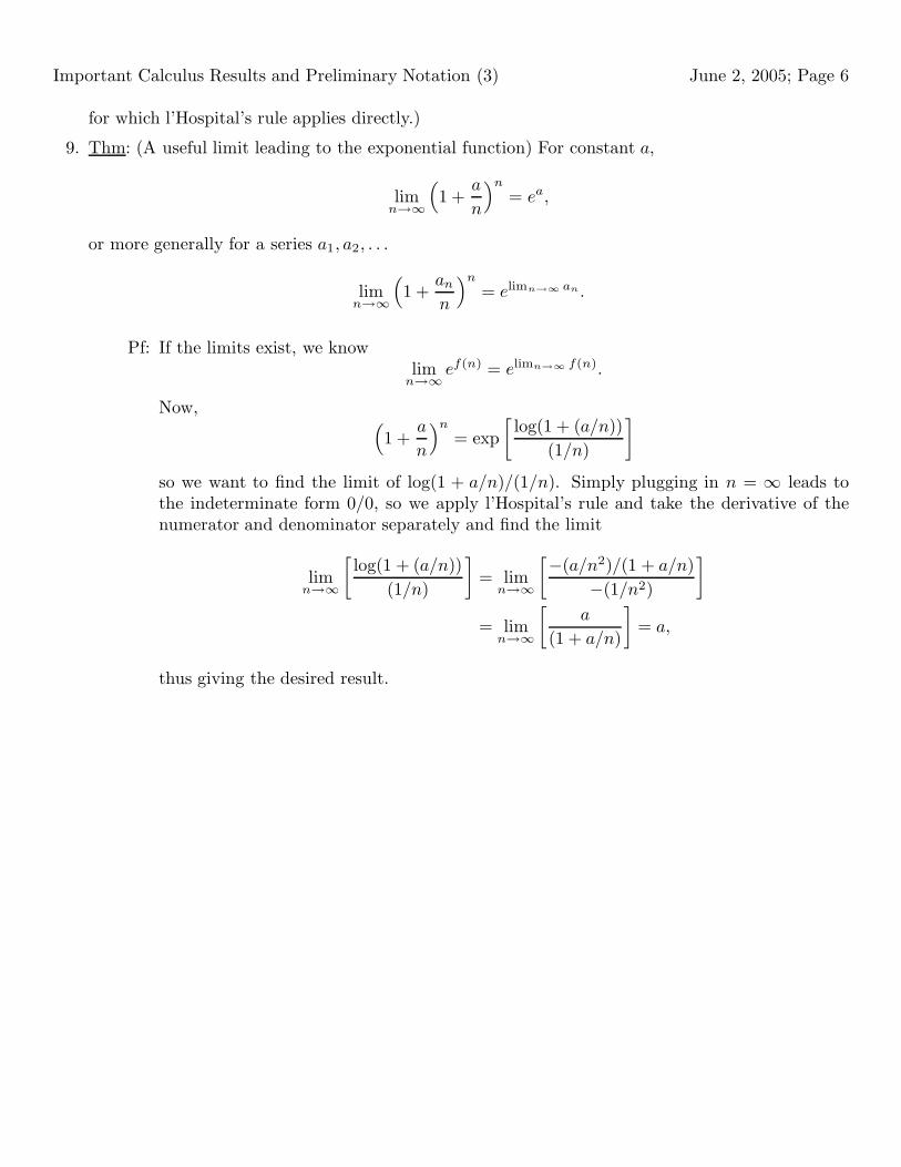
9. Thm: (A useful limit leading to the exponential function) For constant a,

limn→∞

(1 +

a

n

)n

= ea,

or more generally for a series a1, a2, . . .

limn→∞

(1 +

an

n

)n

= elimn→∞ an.

Pf: If the limits exist, we knowlim

n→∞ ef(n) = elimn→∞ f(n).

Now, (1 +

a

n

)n

= exp[log(1 + (a/n))

(1/n)

]

so we want to find the limit of log(1 + a/n)/(1/n). Simply plugging in n = ∞ leads tothe indeterminate form 0/0, so we apply l’Hospital’s rule and take the derivative of thenumerator and denominator separately and find the limit

limn→∞

[log(1 + (a/n))

(1/n)

]= lim

n→∞

[−(a/n2)/(1 + a/n)−(1/n2)

]

= limn→∞

[a

(1 + a/n)

]= a,

thus giving the desired result.

June 2, 2005;

I. General Probability

1. Def: (Axioms of Probability) Given an outcome space Ω, a collection A of subsets of Ω containingΩ and closed under complementation and countable unions, then a real valued function P is aprobability measure if for all Ai ∈ A it satisfies

a. 0 < P(Ai),

b. P(Ω) = 1, and

c. if Ai ∩Aj = ∅ for all i = j (so mutually exclusive events), then P(∪∞i=1Ai) =

∑∞i=1 P(Ai)

2. Thm: (Properties of probablities)

a. P(∅) = 0

b. P(Ac) = 1 − P(A)

c. P(A ∪B) = P(A) + P(B) − P(AB)

d. P(A) = P(A ∩B) + P(A ∩ Bc)

e. P(A ∩B) < P(A)

• (Note: The third and fifth properties are the root cause of the multiple comparison prob-lem.)

3. Def (Conditional Probability) For A,B ∈ A with P(B) > 0, the conditional probability of A givenB is a probability measure

P(A |B) =P(AB)P(B)

4. Thm: (Chain Rule for Joint Probabilities) Given Ai, i = 1, . . . , n, the joint probability can becomputed based on conditional probabilities as

P(∩ni=1Ai) = P(An|A1, . . . , An−1)P(An−1|A1, . . . , An−2) · · · P(A2|A1)P(A1)

= P(A1)n∏

i=2

P(Ai|A1, . . . , Ai−1)

5. Thm: (Probability of an Event by Conditioning on a Partition) Let BiNi=1 be a partition of Ω (so

∪Ni=1Bi = Ω and Bi ∩ Bj = ∅ for all i = j), and further suppose P(Bi) > 0 for all i. Then for all

A ∈ A,

P(A) =N∑

i=1

P(A |Bi)P(Bi).

I. General Probability (2) June 2, 2005;

6. Thm: (Bayes’ Rule) Let BiNi=1 be a partition of Ω, and further suppose P(Bi) > 0 for all i. Then

for all A ∈ A and every k = 1, . . . , n,

P(Bk |A) =P(A |Bk)P(Bk)∑Ni=1 P(A |Bi)P(Bi)

.

7. Def: (Independent Events) Events A and B are independent if P(AB) = P(A)P(B). A collection ofevents B = Bλ : λ ∈ Λ is (totally) independent if for every n and every combination of n distinctelements λi ∈ Λ, i = 1, . . . , n (so λi = λj for i = j) we have

P(∩ni=1Bλi) =

n∏i=1

P(Bλi).

8. Thm: (Properties of independence)

a. If A and B are independent, then P(A|B) = P(A).

• (Note: This is sometimes used as the definition of independence.)

b. If A and B are independent, then so are A and Bc.

9. Note: (Simpson’s Paradox) For events A, B, and C , conditioning simultaneously on events B andC may give qualitatively different results than conditioning on B alone. That is, it is easy to have

P(A |BC) > P(A |BcC)P(A |BCc) > P(A |BcCc)

(that is when C is true, observing event B makes A more likely than when B is not true, and thesame being true when C is not true), but

P(A |B) < P(A |Bc)

(that is, when considering the entire sample space without regard to C , then observing event Bmakes A less likely than when B is not true).

10. Thm: (Sufficient Conditions to Avoid Simpson’s Paradox) For events A, B, and C , with

P(A |BC) > P(A |BcC)P(A |BCc) > P(A |BcCc)

then either of the following conditions

– B and C are independent, OR

– A and C are independent when conditioned on B (so P(AC |B) = P(A |B)P(C |B))

are sufficient (but not necessary) to guarantee

P(A |B) > P(A |Bc)

I. General Probability (3) June 2, 2005;

• (Note: Simpson’s Paradox is the basis for the definition of confounding in applied statis-tics: Given a response variable Y and a predictor of interest X, a third variable W is aconfounder if

– W is causally associated with Y independently of X (so after adjusting for X) in amanner that is not in a causal pathway of interest, AND

– W is causally associated with X.)

June 2, 2005;

II. Random Variables and Distributions

1. Def: (Random Variable) A (quantitative) random variable X is a function X(ω) which maps Ω toR1.

2. Def: (Random Vector) A p dimensional random vector X is a vector of quantitative random variables(X1, . . . ,Xp). (If p = 1, then X is merely a random variable.)

3. Def: (Cumulative distribution function (cdf) and survivor function) A p dimensional random vectorX has cumulative distribution function (cdf) F (x) = Pr[∩p

i=1Xi < xi].4. Note: (Properties of a cdf) A cdf has properties

a. F (x) is nondecreasing in each dimension: For x and y such that xi = yi for all i = k andxk < yk implies F (x) < F (y)

b. F (x) = 0 if xi = −∞ for any i; F (x) = 1 if xi = ∞ for all i.

c. F (x) is continuous from the right: limF (x + h) = F (x) for all x and for all h of the formhi = ε1[i=k] for some 1 < k < p, where the limit is taken as ε decreases to 0.

d. F ( X) must have positive mass over every rectangle.

5. Def: (Probability density function (pdf), probability mass function (pmf))

a. If cdf F (x) is differentiable in all dimensions, f(x) = dF (x)/dx is the probability density function(pdf).

b. If F (x) is a step function, p(x) = F (x) − F (x−) is the probability mass function (pmf), wherewe define F (x−) = limF (x− ε1) as ε→ 0 from above and 1 is a p dimension vector with everyelement equal to 1.

c. By the support of a random vector we mean the set of all x such that the pdf (or pmf) ispositive. Hence, for a continuous random vector, the support might be defined as set

A = x : f X(x) > 0.

Similarly, for a discrete random vector, the support might be defined as set

A = x : p X(x) > 0.

• (Note: We often use the notation f(·) to mean either a pdf or a pmf. Sometimes this iswritten dF (·).)

6. Def: (Marginal Distributions) The marginal cdf of Xk can be found from the joint distribution ofX = (X1, . . . ,Xp) by FXk(x) = F X(y), where yi = ∞ for i = k and yk = x.

II. Random Variables and Distributions (2) June 2, 2005;

a. If X is continuous, the pdf for Xk can be found by integrating the pdf for X over all otherelements.

fXk(x) =∫ ∞

−∞· · ·∫ ∞

−∞f X(y1, . . . , yk−1, x, yk+1, . . . , yp)dy1 . . . dyk−1 dyk+1 . . . dyp

b. If X is discrete, the pmf for Xk can be found by summing the joint pmf for X over all otherelements.

pXk(x) =∑y1

· · ·∑yk−1

∑yk+1

· · ·∑yp

p X(y1, . . . , yk−1, x, yk+1, . . . , yp)

7. Def: (Independence of Random Variables) Two random variables X and Y are independent randomvariables if for all real x, y, the events X < x and Y < y are independent.

• (Note: This definition is based on the definition of independent events, and it demandsthat all pairwise events defined by the random variables are independent.)

8. Thm: (Factorization of Joint Distribution of Independent Random Variables) Two random variablesX1 and X2 are independent if and only if the cdf for X = (X1,X2) can be factored F X(x) =FX1(x1)FX2(x2) for all real valued vectors x = (x1, x2). Similarly, the pdf or pmf of X factors intothe product of the marginal pdf’s or pmf’s.

9. Def: (Conditional pdf or pmf) When fY (y) > 0, the conditional pdf (or pmf) of X given Y = y isdefined as f X|Y (x|Y = y) = f W (w = (x, y))/fY (y), where random vector W = ( X, Y ).

• (Note: The conditional pdf (or pmf) is a pdf (or pmf).)

10. Thm: (Independence via Conditional pdf or pmf) X and Y are independent if and only if theconditional distribution of X given Y = y is f X|Y (x|Y = y) = f X(x) for all x and all y in the

support of Y .

• (Note: Most of inferential statistics about associations proceeds by examining functionals ofconditional distributions. This works because if we can show that some functional (e.g., themean) of f X|Y (x|Y = y1) is different from the corresponding functional of f X|Y (x|Y = y2),

then X and Y cannot be independent. Of course, if the two conditional distributions havethe same value of the functional, that does not prove independence, because it may betrue, for instance, that two distinct conditional distributions have the same mean, but notthe same median.)

June 2, 2005;

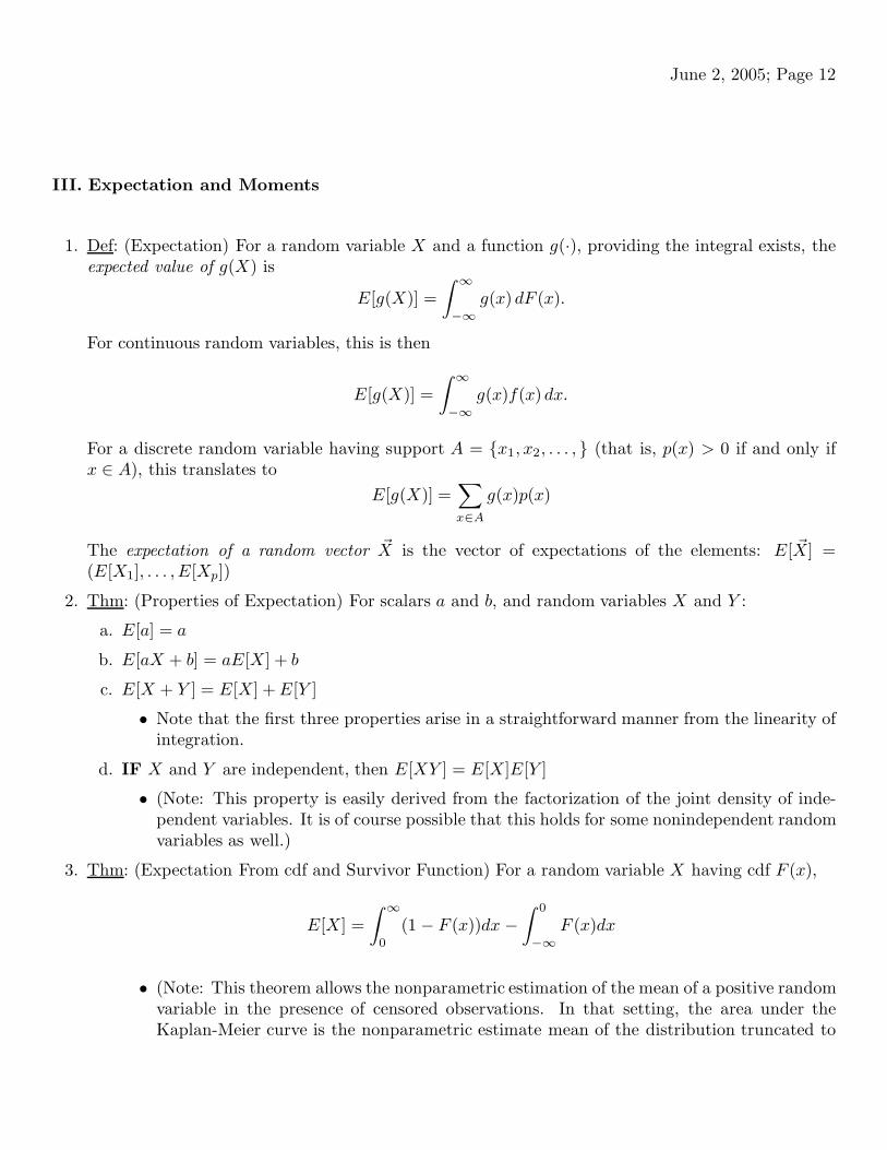
III. Expectation and Moments

1. Def: (Expectation) For a random variable X and a function g(·), providing the integral exists, theexpected value of g(X) is

E[g(X)] =∫ ∞

−∞g(x)dF (x).

For continuous random variables, this is then

E[g(X)] =∫ ∞

−∞g(x)f(x)dx.

For a discrete random variable having support A = x1, x2, . . . , (that is, p(x) > 0 if and only ifx ∈ A), this translates to

E[g(X)] =∑x∈A

g(x)p(x)

The expectation of a random vector X is the vector of expectations of the elements: E[ X] =(E[X1], . . . , E[Xp])

2. Thm: (Properties of Expectation) For scalars a and b, and random variables X and Y :

a. E[a] = a

b. E[aX + b] = aE[X] + b

c. E[X + Y ] = E[X] +E[Y ]

• Note that the first three properties arise in a straightforward manner from the linearity ofintegration.

d. IF X and Y are independent, then E[XY ] = E[X]E[Y ]

• (Note: This property is easily derived from the factorization of the joint density of inde-pendent variables. It is of course possible that this holds for some nonindependent randomvariables as well.)

3. Thm: (Expectation From cdf and Survivor Function) For a random variable X having cdf F (x),

E[X] =∫ ∞

0

(1 − F (x))dx −∫ 0

−∞F (x)dx

• (Note: This theorem allows the nonparametric estimation of the mean of a positive randomvariable in the presence of censored observations. In that setting, the area under theKaplan-Meier curve is the nonparametric estimate mean of the distribution truncated to

III. Expectation and Moments (2) June 2, 2005;

the support of the censoring distribution. Details are beyond the scope of these notes, sosuffice it to say that this is indeed an important property.)

4. Def: (Moments) When the relevant integrals exist:

a. The kth (noncentral) moment of the distribution of random variable X is µ′(k) = E[Xk]. The

first moment is referred to as the mean, and is often denoted by µ.

b. The kth central moment of the distribution of X is µ(k) = E[(X −E[X])k]. The second centralmoment is termed the variance, written V ar(X).

c. For random variables X and Y , we can define joint moments. Of particular interest is thecovariance Cov(X,Y ) = E[(X − E[X])(Y − E[Y ])].

d. The correlation is defined as corr(X,Y ) = Cov(X,Y )/√V ar(X)V ar(Y ).

e. The variance-covariance (or just covariance) matrix for p dimensional random vector X is a pby p dimensional matrix V = [vij ] with vij = Cov(Xi,Xj).

5. Thm: (Properties of Variance and Covariance) For scalars a, b, c, d and random variables W,X, Y, Z:

a. V ar(a) = 0, V ar(X) ≥ 0

b. V ar(X) = E[X2] − E2[X]; Cov(X,Y ) = E[XY ]− E[X]E[Y ]; E[X2] = V ar(X) + E2[X]

c. −1 < corr(X,Y ) < 1

d. V ar(aX + b) = a2V ar(X)

e. Cov(aX + b, cY + d) = acCov(X,Y )

f. V ar(X) = Cov(X,X)

g. Cov(W +X,Y + Z) = Cov(W,Y ) + Cov(W,Z) +Cov(X,Y ) + Cov(X,Z)

h. V ar(X+Y ) = V ar(X)+V ar(Y )+2Cov(X,Y ); V ar(X−Y ) = V ar(X)+V ar(Y )−2Cov(X,Y )

i. IF X and Y are independent, Cov(X,Y ) = 0; corr(X,Y ) = 0, V ar(X + Y ) = V ar(X − Y ) =V ar(X) + V ar(Y )

• (Note: Important distinction: uncorrelated does not necessarily imply independent UN-LESS X and Y are jointly normally distributed.)

6. Thm: (Double Expectation Formula) For random variables X,Y , EY [E[X|Y = y]] = E[X]


Pf: (For the continuous random variable case)

E[X|Y = y] =∫ ∞

−∞xfX|Y (x|y)dx

=∫ ∞

−∞xfX,Y (x, y)fY (y)

dx

EY [E[X|Y = y]] =∫ ∞

−∞

(∫ ∞

−∞xfX,Y (x, y)fY (y)

dx

)fY (y)dy

=∫ ∞

−∞

∫ ∞

−∞xfX,Y (x, y)dxdy

=∫ ∞

−∞x

(∫ ∞

−∞fX,Y (x, y)dy

)dx

=∫ ∞

−∞xfX (x)dx

= E[X]

7. Thm: (Variance via Conditional Distributions) For random variables X,Y , V ar(X) =V arY (E[X|Y ]) + EY [V ar(X|Y )]

Pf: Using the double expectation formula and the standard relation V ar(X) = E[X2] − E2[X]:

V ar(X) = E[X2] − E2[X] = EY [E[X2|Y = y]] −E2Y [E[X|Y = y]]

= EY [V ar(X|Y = y) + E2[X|Y = y]] − E2Y [E[X|Y = y]]

= EY [V ar(X|Y = y)] +(EY [E2[X|Y = y]] − E2

Y [E[X|Y = y]])

= EY [V ar(X|Y = y)] + V arY (E[X|Y = y])

8. Def: (Moment Generating Functions (mgf); characteristic functions (chf))

a. The moment generating function (mgf) (if it exists) for random variable X is MX (t) = E[eXt].

b. The characteristic function (chf) for random variable X always exists and is ψX(t) = E[eiXt].

9. Thm: (Properties of Moment Generating Functions)

a. Two variables having mgf’s have the same probability distribution if and only if they have thesame moment generating functions.

b. The mgf can be expanded as

MX(t) =k∑

i=0

EXi

i!ti + o(tk)

c. The kth derivative of the mgf evaluated at t = 0 is the kth moment of the distribution.


d. The mgf of sums of independent random variables is the product of the marginal mgfs: Forindependent random variables X and Y , the mgf for W = X + Y is MW (t) = MX(t)×MY (t).

e. If Y = aX + b, then MY (t) = ebtMX (at)

f. If Y is a constant, Y = b, then the mgf for Y is MY (t) = ebt

10. Thm: (Properties of Characteristic Functions)

a. Two variables have the same probability distribution if and only if they have the same charac-teristic function.

b. The kth derivative of the characteristic function evaluated at t = 0 is the kth moment of thedistribution divided by (−i)k.

c. The characteristic function of sums of independent random variables is the product of themarginal characteristic functions: For independent random variables X and Y , the mgf forW = X + Y is ψW (t) = ψX (t) × ψY (t).

d. If Y = aX + b, then ψY (t) = eibtψX(at)

e. If Y is a constant, Y = b, then the characteristic function for Y is ψY (t) = eibt

June 2, 2005;

IV. Families of Distributions

1. Def: (Families of Distributions; Parameters) A family of probability distributions is merely a col-lection of cumulative distribution functions. A parametric family of distributions is specified by acdf F (·;λ) where the form of F is known exactly, and where λ ∈ Λ is some parameter for whichknowledge of the exact value is necessary to be able to describe the entire probability distribution.

2. Def: (Binomial Distribution) A random variable X is said to have the Bernoulli distribution withparameter p (notation X ∼ Bernoulli(p) or X ∼ B(1, p)) if Pr[X = 1] = p and Pr[X = 0] = 1− p,and the pmf is zero elsewhere. A random variable X is said to have the binomial distribution withparameters n and p if

Pr[X = k] =(

nk

)pk(1 − p)n−k k ∈ 0, 1, 2, . . . , n

0 else

We write X ∼ B(n, p). Useful properties include

a. E[X] = np.

b. V ar(X) = np(1 − p)

c. The maximum variance for a Binomial random variable occurs when p = 0.5.

d. When n = 1, X has a Bernoulli distribution, and has expectation p and variance p(1 − p).

• Every dichotomous random variable has a Bernoulli distribution. There is no other possi-bility.

e. Distribution of sums of independent binomials (having same success probability): ForX1,X2, . . . ,Xm independently distributed binomial random variables with Xi ∼ B(ni, p) forall i ∈ 1, 2, . . . ,m (note that this allows different values for the n parameter, but requiresthat each of the independent random variables have the same p parameter), then the sum ofthe random variables S =

∑mi=1Xi has a Binomial distribution S ∼ B(n =

∑mi=1 ni, p). In

particular, given m independent, identically distributed Bernoulli random variables (so ni = 1)having the same success probability p, the sum of those independent random variables has thebinomial distribution B(m, p).

3. Def: (Poisson Distribution) A random variable X is said to have the Poisson distribution if

Pr[X = k] =

e−λλk

k! k ∈ 0, 1, 2, . . .0 else

We write X ∼ P(λ). The Poisson distribution can be derived as a count of the number of eventsoccurring over some interval of space and time when

– the events occur at the same rate for each arbitrary interval of space-time,

IV. Families of Distributions (2) June 2, 2005;

– the number of events occurring in disjoint intervals are independent, and

– the probability of observing more than one event in an interval goes to zero as the lengthof the interval decreases.

Useful properties include

a. E[X] = λ

b. V ar(X) = λ

c. Distribution of sums of independent Poissons: For X1,X2, . . . ,Xm independently distributedPoisson random variables with Xi ∼ P(λi) for all i ∈ 1, 2, . . . ,m (note that this allowsdifferent values for the rate parameter λ), then the sum of the random variables S =

∑mi=1Xi

has a Poisson distribution S ∼ P(λ =∑m

i=1 λi). In particular, givenm independent, identicallydistributed Poisson random variables having the same rate parameter λ, the sum of thoserandom variables has the Poisson distribution P(mλ).

d. Given two independent Poisson random variables withX ∼ P(λ) and Y ∼ P(µ), the conditionaldistribution of X conditioned on the sum of X and Y is binomial

X|X + Y = z ∼ B(n = z, p =

λ

λ+ µ

)

4. Def: (Uniform Distribution) A random variableX is said to have the standard uniform (X ∼ U(0, 1))if it has cdf

F (x) = x1(0,1)(x) + 1[1,∞)(x)

More generally, for b > a, X ∼ U(a, b) if it has cdf

F (x) =x− a

b− a1(a,b)(x) + 1[b,∞)(x)

The pdf is

f(x) =1

b− a1(a,b)(x)

Useful properties include

a. E[X] = (b + a)/2; for the standard normal X ∼ U(0, 1), E[X] = 0.5.

b. V ar(X) = (b − a)2/12; for the standard normal X ∼ U(0, 1), V ar(X) = 1/12.

c. Distribution of linear transformed uniforms: If X ∼ U(a, b) and c, d are constants, then if d > 0,c+ dX ∼ U(c+ da, c+ db), and if d < 0, c+ dX ∼ U(c+ db, c+ da).

d. Distribution of log transformed standard uniform: If X ∼ U(0, 1), then for W = −log(X) isdistributed according to an exponential distribution with rate (or mean) parameter 1: W ∼ E(1)(see note ???? below).

• (Note: Under the null hypothesis, P values have a standard uniform distribution (see note??? below). This result is then used to formulate Fisher’s proposal for combining P values


from independent studies: The negative sum of log transformed P values would have agamma distribution, which can further be characterized as a chi-squared distribution.)

5. Def: (Exponential Distribution) A random variable X is said to have the exponential distribution(X ∼ E(λ)) if it has cdf

F (x) = (1 − e−λx)1(0,∞)(x)

and pdff(x) = λe−λx1(0,∞)(x)

and survivor function

S(x) = Pr(X > x) = 1 − F (x) = e−λx1(0,∞)(x)

The above is the “hazard parameterization” of the exponential. The “mean parameterization” has

F (x) = (1 − e−xµ )1(0,∞)(x)

for X ∼ E(µ). You have to be alert to this variation in specification. If λ = 1/µ, these are of coursethe exact same distribution. Useful properties include

a. E[X] = 1/λ = µ

b. V ar(X) = 1/λ2 = µ2

c. Memorylessness property: For s > t, Pr[X > s|X > t] = Pr[X > s − t] and E[X|X > t] =1/λ = µ. (Hence, if an object has an exponentially distributed lifetime, given that it is stillfunctioning at a particular time, it has the same probability of surviving k years into the futureirrespective of its age. The mean residual life expectancy of a currently functioning object(expected number of years before death) is always the same.)

d. Distribution of sums of independent exponentials: For X1,X2, . . . ,Xm independently dis-tributed exponential random variables with Xi ∼ E(λ) for all i ∈ 1, 2, . . . ,m (note thatthis requires the same value for the rate parameter λ), then the sum of the random variablesS =

∑mi=1Xi has a Gamma distribution S ∼ Γ(m,λ, 0) (see note ???? below).

e. Distribution of scale transformed exponentials: If X ∼ E(λ) (hazard parameter λ and meanµ = 1/λ) and c is a constant, then cX ∼ E(λ/c) (so hazard parameter λ/c and mean cµ = c/λ).

6. Def: (Gamma Distribution) A random variable X is said to have the shifted gamma distribution(X ∼ Γ(α, λ,A)) if it has pdf

f(x) =λα

Γ(α)(x− A)α−1e−(x−A)λ1(A,∞)(x)

where Γ(u) =∫∞0 xu−1e−x dx for u > 0. (Note that for n a positive integer, Γ(n) = (n − 1)!.)

Alternative parameterizations exist, so you need to ask what is really meant. Useful propertiesinclude

a. E[X] = α/β + A


b. V ar(X) = α/β2

c. When α = 1 and A = 0 in the above parameterization, X ∼ E(λ), an exponential distributionwith hazard parameter λ.

d. Distribution of sums of independent gammas: For X1,X2, . . . ,Xm independently distributedexponential random variables with Xi ∼ Γ(αi, λ,Ai) for all i ∈ 1, 2, . . . ,m (note that thisrequires the same value for the rate parameter λ, but not the shape parameter α or the locationparameter A), then the sum of the random variables S =

∑mi=1Xi has a Gamma distribution

S ∼ Γ(α =∑m

i=1 αi, λ,A =∑m

i=1Ai)

e. Distribution of location-scale transformed gammas: If X ∼ Γ(α, λ,A) (in the parameterizationwith E[X] = α/λ) and c and d are constants, then cX + d ∼ Γ(α, λ/c, cA + d) (so meanαλ/c+ d).

f. Relationship to chi-quared distribution: If α = 2n where n is a positive even integer, a = 0,and rate parameter λ, then X ∼ Γ(2n, λ, 0) has W = Xλ/2 following a chi-squared distributionwith n degrees of freedom: W ∼ χ2

n (see note ????) below.

7. Def: (Normal Distribution) A random variable X is said to be normally distributed (X ∼ N (µ, σ2))if it has pdf

f(x) =1√2πσ

e−(x−µ)2

σ2 .

A p dimensional random vector X is jointly normally distributed (multivariate normal) with meanµ and symmetric, positive definite covariance matrix Σ (written X ∼ Np(µ,Σ)) if it has pdf

f(x) =1√

2π|Σ|e−(x−µ)T Σ−1(x−µ).

(Note that some authors will consider the case of a degenerate multivariate normal when Σ doesnot have an inverse.) Useful properties include:

a. E[ X] = µ

b. V ar(Xi) = Σii, Cov(Xi,Xj) = Σij .

c. If X ∼ Np(µ,Σ), then for all 1 < i < p, Xi ∼ N (µi,Σii).

d. If X ∼ Np(µ,Σ), then for all 1 < i, j < p, Xi and Xj are independent if and only if Σij = 0.

e. Independent normally distributed random variables are jointly normal.

f. Conditional distributions derived from multivariate normals: Let X ∼ Np(µ,Σ). Further definepartition X = (Y , W ), where Y = (X1, . . . ,Xk) and W = (Xk+1, . . . ,Xn). Similarly definepartitions µ = (µY , µW ),and

Σ =(

ΣY Y ΣY W

ΣWY ΣWW

)

Then Y | W = w ∼ Nk(µY − ΣY W Σ−1WW (w − µW ),ΣY Y − ΣY W Σ−1

WW ΣWY ).


g. Linear transformations of multivariate normals: If X ∼ Np(µ,Σ) and A is a r by p matrix andb is any p dimensional vector, then A X + b ∼ Nr(Aµ + b,AΣAT ). (Note that to make thisstatement in this generality requires allowing degenerate multivariate normal distributions.)

h. Standardization of normal random variables: If X ∼ N (µ, σ2), then Z = (X − µ)/σ hasthe standard normal distribution Z ∼ N (0, 1). (Note that the cdf for a normally distributedrandom variable cannot be solved in closed form, and thus the cdf for the standard normaldistribution tends to be tabulated in textbooks and approximated in most software. We wouldreally need to do numerical integration.)

i. Distributions of sums of independent normals: From the properties specified above, sums ofindependent normals are also normally distributed.

j. Relationship to chi-squared distribution: The chi-squared distribution is defined as the dis-tribution of the sum of squared independent, identically distributed normal random variableshaving variance 1.

k. Quadratic forms: If X ∼ Np(µ,Σ), then Q = ( X − µ)T Σ−1( X − µ) ∼ χ2p.

l. The sample mean and sample variance computed from a sample of independent, identicallydistributed normal random variables are independent.

m. The importance of the normal distribution can not be overstated: The CLT says that sums ofrandom variables tend to be normally distributed as the sample size gets large enough (withsome disclaimers about the random variables having means and the statistical informationtending to infinity).

8. Def: (Chi squared Distribution) For X1,X2, . . . ,Xm independently distributed standard normalrandom variables with Xi ∼ N (0, 1) for all i ∈ 1, 2, . . . ,m, then the sum of the squared randomvariables S =

∑mi=1X

2i has a (central) chi-squared distribution with m degrees of freedom. In the

more general case where X1,X2, . . . ,Xm independently distributed normal random variables withXi ∼ N (µ, σ2) for all i ∈ 1, 2, . . . ,m, then the sum of the squared, scaled random variables S =∑m

i=1(Xi/σ)2 has a noncentral chi-squared distribution withm degrees of freedom and noncentralityparameter µ2/(2σ2). Useful properties include

a. Given a sample of independent, identically distributed normal random variables Xi ∼ N (0, 1)for all i ∈ 1, 2, . . . ,m, then for sample variance s2 =

∑ni=1(Xi − X)2/(n − 1) we know

(n − 1)s2/σ2 ∼ χ2n−1, a chi-squared distribution with n− 1 degrees of freedom.

9. Def: (t Distribution) Given independent random variables Z ∼ N (0, 1) and V ∼ χ2n, then the

distribution of Z/√V/n is called the t distribution with n degrees of freedom. Useful properties

include

a. This result allows the substitution of the estimated standard deviation in place of the populationstandard deviation in many statistics derived from normal distribution models.

b. If T ∼ tn, then T 2 ∼ F1,n, an F distribution with 1 and n degrees of freedom.

10. Def: (F Distribution) Given independent random variables U ∼ χ2m and V ∼ χ2

n, then the distribu-tion of (U/m)/(V/n) is called the F distribution with m,n degrees of freedom. Useful propertiesinclude


a. This result allows the substitution of the estimated variance in place of the population variancein many statistics derived from normal distribution models.

b. If T ∼ tn, then T 2 ∼ F1,n, an F distribution with 1 and n degrees of freedom.

June 2, 2005;

V. Transformations of Random Variables

1. Def: (Monotonicity; Convexity) A function g(x) is said to be

a. monotonically nondecreasing if for all a < b in the domain of g, g(a) < g(b).

b. monotonically increasing if for all a < b in the domain of g, g(a) < g(b).

c. monotonically nonincreasing if for all a < b in the domain of g, g(a) ≥ g(b).

d. monotonically decreasing if for all a < b in the domain of g, g(a) > g(b).

e. monotonic if it is either monotonically nonincreasing or monotonically nondecreasing.

f. strictly monotonic if it is either monotonically increasing or monotonically decreasing.

g. convex if for all a < b in the domain of g and all p ∈ (0, 1), g(pa+(1−p)b) < pg(a)+(1−p)g(b).h. strictly convex if for all a < b in the domain of g and all p ∈ (0, 1), g(pa + (1 − p)b) <

pg(a) + (1 − p)g(b).

i. concave if −g(x) is convex.

j. strictly concave if −g(x) is strictly convex.

2. Thm: (Distribution of Transformed Random Variables) For X a random variable and Y = g(X) forsome real valued function g. Then

FY (y) = Pr[Y < y] = Pr[g(X) < y] = P(ω : g(X(ω)) < y)For discrete rv we find the pmf

Pr[g(X) < y] =∑

x:g(x) < y

p(x)

For continuous rv we find the cdf

Pr[g(X) < y] =∫

x:g(x) < y

f(x)dx

When g(x) is invertible and strictly monotonic

Pr[g(X) < y] = Pr[X < g−1(y)]

3. Thm: (pdf of Transformed Random Variables) If g(x) is differentiable for all x, and either g′(x) > 0or g′(x) < 0 for all x, then for X absolutely continuous and Y = g(X),

f(y) = f(g−1(y))∣∣∣∣ ddy g−1(y)

∣∣∣∣

V. Transformations of Random Variables (2) June 2, 2005;

for y between the minimum and maximum limits of g(x).

4. Thm: (Transformations Based on cdf) For X a random variable with cdf FX , Y = FX(X) hascdf FY (y) = y for all y = FX(x) for some x in the support of X, where the support of X isx : dFX(x) > 0 (for discrete X, dFX(x) is the pmf, for continuous X, dFX(x)isthepdf). Notethat when X is continuous, Y = FX(X) ∼ U(0, 1)

5. Thm: (Transformation Based on Inverse cdf) Let X be a rv with cdf FX and inverse df F−1X . Further

let U ∼ U(0, 1) be a standard uniform rv. Then F−1X (U) ∼ FX (also written F−1

X (U) ∼ X).

6. Thm: (Sums of random variables) Let X = (X1,X2) have joint cdf F X . The cdf for Y = X1 +X2

for discrete rv isFY (y) = Pr[X1 +X2 < y]

=∑x1

∑x2 < y−x1

p X(x1, x2)

The pmf for the sum ispY (y) =

∑x1

p X(x1, y − x1)

If X1 and X2 are independent, the pmf for the sum is the convolution

pY (y) =∑x1

pX1(x1)pX2 (y − x1)

For continuous rv, the cdf for the sum is

FY (y) = Pr[X1 +X2 < y]

=∫ ∞

−∞

∫ y−x1

−∞f X(x1, x2)

and the pdf is found by differentiating to obtain

fY (y) =∫ ∞

−∞f X(x1, y − x1)dx1 =

∫ ∞

−∞f X (y − x2, x2)dx2

If X1 and X2 are independent, the pdf for the sum is the convolution

fY (y) =∫ ∞

−∞fX1(x1)fX2(y − x1)dx1 =

∫ ∞

−∞fX1(y − x2)fX2(x2)dx2

7. Thm: (Differences, products, ratios of random variables) For continuous rv X = (X1,X2),

a. Y = X1 −X2 has

fY (y) =∫ ∞

−∞f X(x1, x1 − y)dx1 =

∫ ∞

−∞f X (y + x2, x2)dx2


b. Y = X1 ×X2 has

fY (y) =∫ ∞

−∞

1|x1|f X(x1, y/x1)dx1 =

∫ ∞

−∞

1|x2|f X(y/x2, x2)dx2

c. Y = X1/X2 has

fY (y) =∫ ∞

−∞|x2|f X(yx2, x2)dx2

8. Thm: (General transformations of continuous random vectors) Let X be a continuous n dimensionalrv, and let Y = (g1( X), . . . , gn( X)) with the gi(x) having continuous first partial derivatives at allx. Define the Jacobian J(y/x) as the determinant of the matrix whose (i, j)-th element is ∂yi/∂xj .Further assume that J(y/x) = 0 at all x. If the pdf f X is continuous at all but a finite number ofpoints, then

fY (y) =f X (x(y))|J(y/x)| 1C(y)

where C is the set of y such that there exists at least one solution for all n equations yi = gi(x).(Note that |J(y/x)| = 1/|J(x/y)|.) Often we desire to transform an n dimensional random vectorto an m dimensional random vector with m < n. To do so we use the above theorem with, say,Yi = Xi for i > m. Then we find the marginal distribution.

9. Thm: (Distribution of order statistics) For a random vector X = (X1, . . . ,Xn), the order statisticsare defined as the permutation of the observations such that X(1) < X(n) < · · · < X(n) (so X(1) isthe minimum of the elements of X , and X(n) is the maximum). If the elements of X constitute arandom sample of i.i.d. random variables with Xi ∼ FX(x) with pdf (pmf) fX (x), then the cdf ofthe kth order statistic is

FX(k)(x) = Pr(X(k) < x)

= Pr(at least k of (X1, . . . ,Xn) are < x)

=n∑

i=k

Pr(exactly i of (X1, . . . ,Xn) are < x)

=n∑

i=k

(ni

)[FX(x)]i[1− FX(x)]n−i

= k(nk

)∫ FX(x)

0

uk−1(1 − u)n−kdu (from integration by parts)

and by differentiation, we find the pdf (pmf) as

fX(k)(x) = k(nk

)fX(x)[FX (x)]k−1 [1 − FX(x)]n−k

• (Note: The most important of the order statistics are, of course, the minimum and maxi-mum. The cdf for these order statistics are most easily derived from


– (cdf for sample minimum of n continuous i.i.d. rv’s)

FX(1)(x) = 1 − Pr[X(1) > x]

= 1 − Pr[X1 > x,X2 > x, · · · ,Xn > x]= 1 − (1 − FX(x))n

– (cdf for sample maximum of n continuous i.i.d. rv’s)

FX(n)(x) = Pr[X(n) < x]

= Pr[X1 < x,X2 < x, · · · ,Xn < x]= (FX (x))n

In either case, the pdf can be obtained by differentiation. For discrete rv’s, the sameapproach can be used, but we have to consider the probability mass at x.)

10. Thm: (Jensen’s Inequality) Let g(x) be a convex function. Then for random variable X, E[g(X)] ≥g(E[X]). If g(X) is strictly convex, then E[g(X)] > g(E[X]).

• (Note: The direction of the inequality is easy to remember by the following: g(x) = x2 isconvex, and because variances must be nonegative, E[X2] − E2[X] ≥ 0.)

June 2, 2005;

VI. Asymptotic Results

1. Def: (Definitions of convergences)

a. Convergence of a series: A series of reals a1, a2, . . . converges to real a

an → a iff ∀ε > 0 ∃nε : ∀n > nε |an − a| < ε

b. Convergence almost surely: A series of random variables X1,X2, . . . converges almost surely torandom variable X

Xn →as X iff Pr [ω ∈ Ω : Xn(ω) → X(ω)] = 1

c. Convergence in probability: A series of random variables X1,X2, . . . converges in probabilityto random variable X

Xn →p X iff ∀ε > 0 Pr [ω ∈ Ω : |Xn(ω) −X(ω)‖ < ε] → 1

d. Convergence in mean square (L2): A series of random variables X1,X2, . . . converges in meansquare to random variable X

Xn →L2 X iff E[(Xn −X)2] → 0

e. Convergence in distribution: A series of random variables X1,X2, . . . having cumulative distri-bution functions F1, F2, . . ., respectively, converges in distribution to random variable X havingcumulative distribution F

Xn →d X iff ∀x such that F is cts at x Fn(x) → F (x)

2. Thm: (Convergence implications) For real numbers a, a1, a2, . . . and random variables X,X1,X2, . . .

a. an → a implies an →as a

b. Xn →as X implies Xn →p X

c. Xn →L2 X implies Xn →p X

d. Xn →p X implies Xn →d X

e. Xn →d a (a constant) implies Xn →p a

3. Thm: (Properties of Convergence in Probability) For random variables X,X1,X2, . . . andY, Y1, Y2, . . .

VI. Asymptotic Results (2) June 2, 2005;

a. Xn →p X iff Xn −X →p 0

b. if Xn →p X and Yn →p Y , then Xn ± Yn →p X ± Y and XnYn →p XY

c. if Xn →p X and g is a continuous function, then g(Xn) →p g(X)

4. Thm: (Chebyshev’s Inequality) For any random variable X having E[X] = µ and variance σ2 <∞,and any ε > 0

Pr[|X − µ| > ε] <σ2

ε2

Pf:

V ar(X) =∫ ∞

−∞(x− µ)2dF (x)

=∫ µ−ε

−∞(x− µ)2dF (x) +

∫ µ+ε

µ−ε

(x− µ)2dF (x) +∫ ∞

µ+ε

(x− µ)2dF (x)

ge

∫ µ−ε

−∞ε2dF (x) +

∫ µ+ε

µ−ε

0dF (x) +∫ ∞

µ+ε

ε2dF (x)

= ε2Pr[|X − µ| > ε]

5. Thm: (Laws of Large Numbers)

a. Weak Law of Large Numbers: For i.i.d. random variables X1,X2, . . . having E[Xi] = µ andvariance V ar(Xi) = σ2 < ∞, then for the series of sample means Xn = 1

n

∑ni=1Xi satisfies

Xn →p µ.

Pf: From simple properties of expectation we have E[Xn] = µ and V ar(Xn) = σ2/n. Thenby Chebyshev’s inequality,

∀ε > 0, P r[|Xn − µ| > ε] <σ2

nε2→ 0

thus satisfying the definition for Xn →p µ.

b. Khinchin’s Theorem: For i.i.d. random variables X1,X2, . . . having E[Xi] = µ < ∞, then forthe series of sample means Xn = 1

n

∑ni=1Xi satisfies Xn →p µ.

Pf: (Using moment generating functions) Because Xn is a sum of independent random vari-ables Xi/n, using the properties of moment generating functions

MXn(t) =

[MX1

(t

n

)]n

=[1 + µ

t

n+ o

(t

n

)]n

=[1 +

µt + no(t/n)n

]n

→ eµt,


which is the moment generating function for the constant µ.

6. Thm: (Central Limit Theorems)

a. (Levy Central Limit Theorem) For i.i.d. random variables X1,X2, . . . having E[Xi] = µ andvariance V ar(Xi) = σ2 < ∞, then for the series of sample means Xn = 1

n

∑ni=1Xi satisfies√

n(Xn − µ) →d N (0, σ2).

Pf: (Using moment generating functions) Because Zn =√n(Xn − µ)/σ is a sum of the in-

dependent random variables (Xi − µ)/(√nσ), using the properties of moment generating

functions

MZn(t) =[MX1−µ

(t√nσ

)]n

=[1 +

E[X1 − µ]1!

t√nσ

+E[X1 − µ]2

2!t2

nσ2+ o

(t2

nσ2

)]n

=

1 +

12 t

2 + no(

t2

nσ2

)n

n

→ e12 t2 ,

which is the moment generating function for the standard normal distribution. The resultthen follows by the uniqueness of the moment generating function. (Note: mgf’s do notalways exist, but a similar proof can be used with chf’s.)

b. (Multivariate Central Limit Theorem) For i.i.d. random vectors X1, X2, . . . having E[ Xi] = µ

and variance-covariance matrix Cov( Xi) = Σ, then the series of sample means Xn = 1n

∑ni=1

Xi

satisfies √n( Xn − µ) →d N (′,±).

c. (Central Limit Theorems for non-identically distributed RVs) Let X1,X2, . . . be independentrandom variables with E[Xi] = µi, var(Xi) = σ2

i . Define Sn =∑n

i=1Xi, µ(n) =∑n

i=1 µi,σ2

(n) =∑n

i=1 σ2i .

– (Liapunov Central Limit Theorem) Let E[(Xi − µi)3] = γi and define γ(n) =∑n

i=1 γi. Ifγ(n)/σ

3(n) → 0 as n→ ∞, then

Sn − µ(n)

σ(n)→d N (0, 1)

– (Lindeberg-Feller Central Limit Theorem) Both

· Sn/σ(n) →d N (0, 1), and

· limn→∞ maxσ2i /σ

2(n), 1 ≤ i ≤ n = 0

if and only if (the Lindeberg condition)

∀ε > 0 limn→∞

1σ2

(n)

n∑i=1

E[|Xi|21[|Xi|≥εσ(n)]

]= 0


7. Thm: (Asymptotic Distributions of Transformations of Random Variables)

a. (Continuous Mapping Theorem (Mann-Wald)) If g is a continuous function almost surely(i.e., the probability of the set where g is not continuous is zero), then for random variablesX,X1,X2, . . ., Xn →d X implies g(Xn) →d g(X).

• (Note: When used with statistics having the usual form of a(n)(Tn − θ) →d Z, the Mann-Wald theorem also transforms the normalizing function a(n). We usually are not as in-terested in such a transformation unless it is absolutely necessary to avoid a degeneratedistribution.)

b. (Slutsky’s Theorem) If an →p a, bn →p b, and Xn →d X are convergent series of randomvariables, then anXn + bn →d aX + b.

• (Note: Slutsky’s Theorem is useful when desiring to replace an unknown parameter witha consistent estimate, e.g., substituting an estimated variance for an unknown variance inan asymptotic distribution.)

c. (Delta Method) If g is a differentiable function at θ (so g′(θ) exists) and an → ∞ as n → ∞,then for random variables X,X1 ,X2, . . .

an(Xn − θ) →d X implies an(g(Xn) − g(θ)) →d g′(θ)x.

A multivariate delta method also exists: If g is a real valued function taking vector argumentand g has a differential at θ and an → ∞ as n→ ∞, then

an(Zn − θ) →dZ implies an(g(Zn) − g(θ)) →d grad g(θ) · Z,

where gradg =(

∂g∂θ1

, . . . , ∂g∂θp

).

• (Note: The Delta Method is useful when desiring to transform an estimator, withouttransforming the normalizing function of n, e.g., when finding an asymptotic distributionfor X

2

n.)

8. Note: (Recipes for finding asymptotic distributions) In statistics we are most often interested infinding statistics which “consistently” estimate unknown parameters (i.e., statistics which convergein probability to the unknown parameter) and in finding the asymptotic distribution of some nor-malized form of the statistic.

a. Methods for establishing convergence in probability

– Brute force using the definition of convergence in probability (often via Chebyshev’s in-equality)

– De novo using the WLLN for a sum of i.i.d. random variables

– Using convergence implications (e.g., using convergence almost surely, convergence in meansquare, or convergence in distribution to a constant)

– Transforming a statistic(s) already known to converge in probability using the propertiesof convergence in probability


b. Methods for finding the asymptotic distribution of a normalized statistic: Given some statistic(estimator) Tn, we usually find the asymptotic distribution for some normalization of the forma(n)[Tn − θ]. (The most commonly used normalization is where a(n) =

√(n) and θ = E[Tn].)

– Brute force using the definition of convergence in distribution

– Using limits of moment generating functions or characteristic functions

– De novo using a CLT for a sum of random variables

– Using convergence implications

– Transformations of statistic(s) already known to converge in distribution (and possiblystatistics known to converge in probability) using Mann-Wald, the Delta Method, andSlutsky’s

9. Ex: (Illustrative examples to show convergence in probability)

a. Brute force: Proof of WLLN uses Chebyshev’s inequality and the definition of convergence inprobability.

b. Convergence implications: Proof of Khinchin’s uses mgf to show convergence in distribution toa constant, then convergence implications to establish convergence in probability.

c. Transformations of sample means: Establishing the consistency of the sample standard devia-tion as an estimator of the population standard deviation.

Suppose X1,X2, . . . are i.i.d. random variables with mean µ and variance σ2.

– Because σ2 = E[(Xi − µ)2], Khinchin’s theorem tells us that

Tn =1n

n∑i=1

(Xi − µ)2 →p σ2

• Since (Xi − µ)2 = (Xi −Xn +Xn − µ)2,

1n

n∑i=1

(Xi − µ)2 =1n

n∑i=1

(Xi −Xn)2 +1n

(Xn − µ)n∑

i=1

(Xi −Xn)

+1n

n∑i=1

(Xn − µ)2

=1n

n∑i=1

(Xi −Xn)2 + (Xn − µ)2

– By the WLLN, Xn →p µ, and by properties of convergence in probability this impliesXn − µ→p 0. The continuous mapping theorem then tells us that (Xn − µ)2 →p 02 = 0.From these results, we get that

1n

n∑i=1

(Xi −Xn)2 =1n

n∑i=1

(Xi − µ)2 − (Xn − µ)2 →p σ2 − 0 = σ2


– Now, n/(n− 1) → 1, so by Slutsky’s theorem

n

n− 11n

n∑i=1

(Xi −Xn)2 = s2 →p 1 × σ2 = σ2

– A final application of the continuous mapping theorem with the square root functionprovides s→p σ, so the sample standard deviation is consistent for the population standarddeviation.

10. Ex: (Illustrative examples to show convergence in distribution)

a. Brute force: Establishing the asymptotic distribution of n(θ−X(n)), whereX(n) is the nth orderstatistic (i.e., maximum) of a sample X1, . . . ,Xn of i.i.d. uniform U(0, θ) random variables.Noting that the cdf for Xi is FXi(x) = x/θ1(0,θ)(x) + 1[θ,∞)(x),

FX(n)(x) =(xθ

)n

1(0,θ)(x) + 1[θ,∞)(x).

NowPr[n(θ −X(n)) < y] = Pr[X(n) > θ − y

n]

= 1 − FX(n)(θ −y

n])

= 1 −[1 − y

nθ

]n1(0,nθ)(y) − 1(−∞,0](y)

= 1(0,∞)(y) −[1 − y

nθ

]n1(0,nθ)(y)

Taking the limit as n→ ∞, because limn→∞(1 + a/n)n = ea, we find

Pr[n(θ −X(n)) < y] → [1 − e−y/θ ]1(0,∞)(y).

Thusn(θ −X(n)) →d E(

1θ),

an exponential distribution with mean θ.

b. Using mgf or chf: The Levy CLT was proved using mgf.

c. Using the CLT: The asymptotic distribution of the sample proportion. For i.i.d Bernoulli(p)random variables X1,X2, . . ., E[Xi] = p and V ar(Xi) = p(1 − p). By the CLT, we thus havethat

p =1n

n∑i=1

Xi

satisfies √n

(p− p)√p(1 − p)

→d N (0, 1).


d. Using transformations: Now, by the WLLN p→p p, so√p(1 − p)/

√p(1 − p) →p 1 and

√n

(p − p√p(1 − p)

→d N (0, 1).

e. Using delta method: The asymptotic distribution of the log odds ratio. Given totally indepen-dent random samples of Bernoulli random variables X1,X2, . . . ,Xn and Y1, Y2, . . . , Yn, whereXi ∼ B(1, pX) and Yi ∼ B(1, pY ), we commonly base comparisons between the distributions on

· the difference in proportions pX − pY ,

· the ratio of proportions pX/pY , or

· the odds ratio (pX/(1 − pX))/(pY /(1 − pY )).

Although it is less straightforward, the odds ratio has several advantages in epidemiologicstudies. Typically, when inference is desired for a ratio, we actually make inference on the scaleof the log odds ratio, because differences are statistically more stable than ratios. Hence, wewant to find an asymptotic distribution of the log odds ratio. (For notational convenience, wedefine qX = 1 − pX and qY = 1 − pY , and we denote the sample means pX =

∑ni=1Xi/n and

pY =∑n

i=1 Yi/n.)

– We first note that the joint distribution of (Xi, Yi) has mean vector and covariance matrix

(Xi

Yi

)∼((

pX

pY

),

(pXqX 0

0 pY qY

)).

– The multivariate CLT thus tells us that the sample mean (pX , pY )T has asymptotic dis-tribution √

n

((pX

pY

)−(pX

pY

))→d N2(0,Σ)

– Now, g(x) = log(x1/(1 − x1)) − log(x2/(1 − x2)), has gradient vector

∇g(x) =

(1

x1(1−x1)

1x2(1−x2)

).

Hence, by the multivariate delta method we have

√n

(log(pX qYqX pY

)− log

(pXqYqXpY

))→d N (

0,∇gT (p)Σ∇g(p))= N

(0,

1pXqX

+1

pY qY

).

June 2, 2005;

VII. Elements of a Statistical Problem

1. Def: (Random Sample) A random sample is an observation X = x drawn at random from theprobability distribution F X .

a. We often consider a one sample setting in which X = (X1, . . . ,Xn) satisfies Xi ∼ FX fori = 1, . . . , n and F X(x) =

∏ni=1 FX(xi) for all x ∈ Rn (i.e., the X ′

is are totally independentand identically distributed). This is often termed a simple random sample and described asX1, . . . ,Xn are i.i.d. with Xi ∼ FX (where ‘i.i.d.’ stands for independent and identicallydistributed).

2. Def: (Functional)

3. Def: (Statistical Estimation Problem)

4. Def: (Statistical Testing Problem)

5. Def: (Regression Problem)

6. Def: (Parametric, Semiparametric, and Nonparametric Statistical Problems)

June 2, 2005;

VIII. General Frequentist Estimation

1. Def: (Statistical Estimation Problem, Functional) In a statistical estimation problem, we have ob-served data X having probability distribution F X , and we desire to estimate some functional θof F X . A functional of the distribution is merely any quantity that can be computed from theprobability distribution function.

• Examples of commonly used functionals might be related to the mean(s) or median(s) ofthe marginal distributions of the elements of X, the probabilities with which the elementsof X exceed some particular threshold, the hazard function

Statistical estimation problems are often characterized as

a. a parametric statistical model in which it is presumed that F X = F X(x; µ)

2. Def: (Statistic, Estimator, Distribution of Estimators; Standard Errors) A statistic is any functionof observed random variables and known quantities (i.e., a statistic cannot involve an unknownparameter, though it can involve hypothesized parameters). A statistic which is used to estimatesome unknown parameter is an estimator. A point estimate is a statistic used to give the single“best” estimate of the unknown parameter, and an interval estimate indicates a range of valuesthat are in some sense reasonable estimates of the unknown parameter. The sampling distributionof an estimator is the probability distribution of the statistic. In the frequentist interpretation ofprobability, the sampling distribution is viewed as the distribution of statistics computed from alarge number of (at least conceptual) replications of the experiment. The standard deviation ofthe sampling distribution for an estimator is termed the standard error of the estimate in orderto distinguish it from the standard deviation of the underlying data. (Sampling distributions ofestimators are important when trying to determine the optimality of frequentist point estimators,when trying to obtain frequentist interval estimates (confidence intervals), and when trying toconstruct hypothesis tests based on an estimator.)

a. Because a statistic is a function of random variables, the exact sampling distribution of anestimator can sometimes be derived using theorems about transformations of random variables.

• (Example: For i.i.d Bernoulli(p) random variables X1,X2, . . ., the consistency of p (seeVI.13.c) might suggest that p is therefore a reasonable estimator of p. Noting that p =∑n

i=1Xi/n, allows us to immediately deduce that Tn = np has the binomial distributionTn ∼ B(n, p) (see IV.2), thus providing the distribution of p.)

b. Sometimes when the exact probability distribution of an estimator is somewhat complicatedto derive we can still find the first two moments (mean and variance) of the sampling distribu-tion. Such knowledge is often sufficient to establish some of the optimality properties for theestimator.

• (Example: For i.i.d. random variables X1,X2, . . . with mean E[Xi] = µ and varianceV ar(Xi) = σ2, we know that the sample mean has a probability distribution with mean

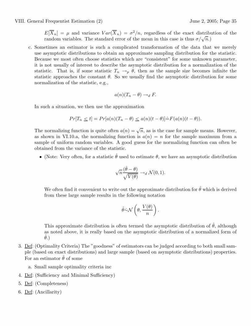
VIII. General Frequentist Estimation (2) June 2, 2005;

E[Xn] = µ and variance V ar(Xn) = σ2/n, regardless of the exact distribution of therandom variables. The standard error of the mean in this case is thus σ/

√n.)

c. Sometimes an estimator is such a complicated transformation of the data that we merelyuse asymptotic distributions to obtain an approximate sampling distribution for the statistic.Because we most often choose statistics which are “consistent” for some unknown parameter,it is not usually of interest to describe the asymptotic distribution for a normalization of thestatistic. That is, if some statistic Tn →p θ, then as the sample size becomes infinite thestatistic approaches the constant θ. So we usually find the asymptotic distribution for somenormalization of the statistic, e.g.,

a(n)(Tn − θ) →d F.

In such a situation, we then use the approximation

Pr[Tn < t] = Pr[a(n)(Tn − θ) < a(n)(t − θ)]=F (a(n)(t − θ)).

The normalizing function is quite often a(n) =√n, as is the case for sample means. However,

as shown in VI.10.a, the normalizing function is a(n) = n for the sample maximum from asample of uniform random variables. A good guess for the normalizing function can often beobtained from the variance of the statistic.

• (Note: Very often, for a statistic θ used to estimate θ, we have an asymptotic distribution

√n

(θ − θ)√V (θ)

→d N (0, 1).

We often find it convenient to write out the approximate distribution for θ which is derivedfrom these large sample results in the following notation

θ∼N(θ,V (θ)n

).

This approximate distribution is often termed the asymptotic distribution of θ, althoughas noted above, it is really based on the asymptotic distribution of a normalized form ofθ.)

3. Def: (Optimality Criteria) The ”goodness” of estimators can be judged according to both small sam-ple (based on exact distributions) and large sample (based on asymptotic distributions) properties.For an estimator θ of some

a. Small sample optimality criteria inc

4. Def: (Sufficiency and Minimal Sufficiency)

5. Def: (Completeness)

6. Def: (Ancillarity)

VIII. General Frequentist Estimation (3) June 2, 2005;

7. Thm: (Basu)

8. Thm: (Cramer-Rao Lower Bound)

9. Thm: (BRUE)

10. Thm: (Rao-Blackwell)

11. Thm: (Lehmann-Scheffe)

June 2, 2005;

VIII. Methods of Finding Estimators

1. Note: (General Approaches)

2. Def: (Method of Moments Estimation)

3. Thm: (General Optimality of MME)

4. Thm: (Maximum Likelihood Estimation)

5. Thm: (Regular MLE Theory)

6. Thm: (Optimality of MLE)

7. Def: (Exponential Families)

8. Note: (Exponential Family and Complete Sufficient Statistics)

9. Note: (Recipes for Finding UMVUE)

10. Note: (Nonparametric Estimation)

June 2, 2005;

IX. Frequentist Hypothesis Testing

1. Note: (Testing Problem)

2. Def: (Decision Rule)

3. Def: (Type I, II Errors, Power)

4. Thm: (Neyman-Pearson Lemma)

5. Def: (Monotone Likelihood Ratio)

6. Thm: (Karlin-Rubin)

7. Thm: (Asymptotic Likelihood Theory in Regular Problems)

8. Thm: (Intuitive Tests Based on Normal Estimators)

June 2, 2005;

X. Frequentist Confidence Intervals

1. Def: (Confidence Interval)

2. Def: (Pivotal Quantity)

3. Note: (CI via Pivotal Quantity)

4. Note: (CI via Inverting Test)

5. Note: (CI Based on Normal Estimators)

June 2, 2005;

XI. Bayesian Inference

1. Note: (Bayesian Paradigm)

2. Def: (Prior and Posterior Distributions)

3. Def: (Conjugate Prior Distribution)

4. Def: (Loss, Risk, Bayes Risk)

5. Thm: (Bayes estimator with Squared Error Loss)

6. Def: (Credible Intervals)

7. Ex: (Normal with Conjugate Prior)

an overview of mathematical statistics (top 10 lists) · an overview of mathematical statistics...

Documents