an optimization approach for well-targeted transcranial...

SIAM J. APPL. MATH. c© 2016 Society for Industrial and Applied MathematicsVol. 76, No. 6, pp. 2154–2174

AN OPTIMIZATION APPROACH FOR WELL-TARGETEDTRANSCRANIAL DIRECT CURRENT STIMULATION∗

SVEN WAGNER† , MARTIN BURGER‡ , AND CARSTEN H. WOLTERS†

Abstract. Transcranial direct current stimulation (tDCS) is a noninvasive brain stimulationtechnique which modifies neural excitability by providing weak currents through scalp electrodes.The aim of this study is to introduce and analyze a novel optimization method for safe and well-targeted multiarray tDCS. For optimization, we consider an optimal control problem for a Laplaceequation with Neumann boundary conditions with control and pointwise gradient state constraints.We prove well-posedness results for the proposed methods and provide computer simulation resultsin a highly realistic six-compartment geometry-adapted hexahedral head model. For discretizationof the proposed minimization problem the finite element method is employed and the existence ofat least one minimizer to the discretized optimization problem is shown. For numerical solution ofthe corresponding discretized problem we employ the alternating direction method of multipliers andcomprehensively examine the cortical current flow field with regard to focality, target intensity, andorientation. The numerical results reveal that the optimized current flow fields show significantlyhigher focality and, in most cases, higher directional agreement to the target vector in comparisonto standard bipolar electrode montages.

Key words. transcranial direct current stimulation, optimization, Neumann boundary control,gradient state constraint, sparsity optimal control, existence

AMS subject classifications. 92C50, 78M50, 49N90, 49M29, 35Q93

DOI. 10.1137/15M1026481

1. Introduction. Transcranial direct current stimulation (tDCS) is a nonin-vasive, inexpensive, and easy-to-perform brain stimulation technique which modifiesneural excitability [24]. Changes in neural membrane potentials are induced in apolarity-dependent manner; for example, in a motor cortex study, anodal stimulationright over the motor cortex enhances cortical excitability, whereas cathodal stimula-tion inhibits it [24]. Recently, tDCS has been applied successfully in the treatment ofneurological and neuropsychiatric disorders such as epilepsy [14], depression [6], andAlzheimer’s disease [13]. The effects of tDCS can be preserved for more than one hourafter stimulation [23].

The conventional strategy is to apply the current density σ∇Φ via two large elec-trodes, with the active electrode (anode) to be placed above the presumed targetregion and the reference electrode (cathode) far away from the target region [24, 23].Accurate and detailed finite element (FE) head models have been created to inves-tigate the induced current density distribution [32, 10, 29]. While significant effectsof stimulation as compared to sham were reported [6, 14, 24], computer simulationstudies have revealed that the induced cortical current flow fields are very widespread

∗Received by the editors June 19, 2015; accepted for publication (in revised form) August 29,2016; published electronically November 1, 2016.

http://www.siam.org/journals/siap/76-6/M102648.htmlFunding: The research of the first and third authors was supported by the priority program

SPP1665 of the German Research Foundation, project WO1425/5-1. The second author’s researchwas supported by the ERC via grant EU FP 7 - ERC Consolidator grant 615216 LifeInverse and bythe German Science Foundation DFG via EXC 1003 Cells in Motion Cluster of Excellence, Munster,Germany.†Institute for Biomagnetism and Biosignalanalysis, Westfalische Wilhelms-Universitat Munster,

D 48149 Munster, Germany (s [email protected], [email protected]).‡Institute for Computational and Applied Mathematics, Westfalische Wilhelms-Universitat

Munster, D 48149 Munster, Germany ([email protected]).

2154

http://www.siam.org/journals/siap/76-6/M102648.html

mailto:[email protected]



tDCS OPTIMIZATION APPROACH 2155

with often strongest current density amplitudes in nontarget brain regions [32, 29].It is therefore a matter of debate whether the effects of stimulation are driven by thetarget brain region or elicited by adjacent cortical lobes [29].

In order to overcome the limitations of conventional bipolar electrode montages,algorithmic-based sensor optimization approaches were presented [10, 29, 21, 28]. Imet al. [21] searched for two electrode locations which generate maximal current flow to-wards a certain target direction. Ruffini et al. [28] described a method for optimizingthe configuration of multifocal transcranial current simulation (tCS) for stimulationof brain networks, represented by spatially extended cortical targets. Dmochowskiet al. [10] used a multichannel array consisting of 64 fixed electrode locations to cal-culate optimized stimulation protocols for presumed target regions. They employedradial and tangential targets and reported that compared with conventional electrodemontages their optimization approach achieved electric fields which exhibit simulta-neously greater focality and target intensity at cortical targets using the same totalcurrent applied.

While the optimization results are very promising and a pilot study using multi-array tDCS devices for rehabilitation after a stroke has been conducted [11], to ourknowledge, there is currently no study providing an in-depth analysis of mathematicalmodels for multiarray tDCS optimization.

Given a volume conductor model Ω with a fixed electrode arrangement and atarget vector e in Ωt with Ωt ⊂ Ω being the target cortical area, the optimizationapproach estimates an optimal applied current pattern at the fixed electrodes. ALaplace equation with inhomogeneous Neumann boundary conditions is used to cal-culate the induced current density distribution [32] which is to be controlled by theboundary condition to ensure safe and focused stimulation. Therefore, the optimiza-tion problem for tDCS is in the class of control problems with Neumann boundaryconditions [22].

In this paper, we modeled the electrodes with the point electrode model (PEM)[26, 1, 2]. They can, however, also be modeled using a complete electrode model(CEM) [26, 9, 12, 1, 2]. In [1, 2], it has been shown that the CEM and PEM only leadto small differences which are mainly situated locally around the electrodes and arevery small in the brain region. Based on these results, the application of the PEMis expected to result in negligible differences to the CEM and should thus provide asufficiently accurate modeling of the current density within the brain region.

This paper is organized as follows: In section 2 we establish the mathematicalmodel of tDCS and introduce the optimization problem for multichannel tDCS. Insection 3 we show the existence of at least one minimizer to the optimization problemand the finite element method (FEM) is used for numerical discretization. In section4 we derive the algorithm for sensor optimization. Section 5 provides optimizationresults in a highly realistic six-compartment head model (skin, skull compacta, skullspongiosa, CSF, and gray and white matter) with white matter anisotropy. Further-more, a conclusion and outlook section is presented.

2. Mathematical model of tDCS. In order to calculate the current flow fieldinduced by tDCS, the quasi-static approximation to Maxwell’s equations is applied[32]. This yields the tDCS forward problem

∇ · σ∇Φ = 0 in Ω,

〈σ∇Φ,n〉 = I on Γ ⊂ ∂Ω,

Φ = 0 on ΓD = ∂Ω \ Γ

2156 SVEN WAGNER, MARTIN BURGER, AND CARSTEN H. WOLTERS

with Φ being the electric potential, σ ∈ (L∞)3×3 being an anisotropic conductivitytensor, I being the applied current pattern at the electrodes with nonzero values onlyat the electrode surfaces, n being the outward normal vector, and Γ being a part ofthe boundary of the domain Ω. Furthermore, a Dirichlet boundary condition on theremaining part ΓD is used to ensure that a solution to the tDCS forward problem isunique. We assume all parts of the boundary to have nonzero measure and to be ofLipschitz regularity. We introduce the Sobolev space

H− 1

2 (Γ) :=

u ∈ H− 1

2 (Γ)|∫

Γ

u(s) ds = 0

⊂ H− 1

2 (Γ)

with H−12 (Γ) being the standard Sobolev space for Neumann boundary values on Γ.

The precise definition of H−12 (Γ) is to be the dual space of H

12 (Γ) consisting of the

Dirichlet traces of H1-functions in Ω. The integral in the above definition has to beinterpreted as a duality product with the constant function equal to one, which is inH

12 (Γ). The weak formulation of the forward problem is given by∫

Ω

σ∇Φ · ∇Ψ dx =

∫Γ

I Ψ dσ

for all test functions Ψ ∈ H1(Ω) with vanishing Dirichlet trace on ΓD. Note that theboundary integral on the right-hand side is only defined if I ∈ L2(Γ); in general, it is

to be replaced by the duality product between H−12 (Γ) and H

12 (Γ).

Under standard and naturally satisfied regularity assumptions, there exists aunique solution Φ ∈ H1(Ω) to the tDCS forward problem, which can be shown by theLax–Milgram lemma.

Theorem 2.1. Let σ ∈ (L∞)3×3 with σ ≥ σ0I3×3, and let I ∈ H−12

(Γ). Thenthere exists a solution Φ ∈ H1(Ω) to the tDCS forward problem. The solution isunique if ΓD has positive measure. Moreover, the following norm estimate holds:

‖Φ‖H1 ≤ C ‖I‖H−

12.

For current density optimization, a multichannel array consisting of 74 fixed elec-trode locations (the locations of an extended 10-10 EEG electrode system) is usedand optimized applied current patterns are calculated for presumed targets. Figure1 illustrates an overview of the optimization setup in a two-dimensional model. Op-timally, the induced current density distribution is maximal in the target region Ωtand zero in nontarget regions Ωr = Ω \ Ωt. Physically, a focal stimulation withoutstimulating nontarget regions is not possible, as the current has to flow through thevolume to reach the target region. Therefore, the current density is restricted by ε > 0such that

|σ∇Φ| ≤ ε in Ωr.

Second, the total current applied to all electrodes is limited to 2 mA, a commonlyused safety criterion [10].

For effective stimulation, the optimized current density distribution should beoriented perpendicularly to the cortical surface [5, 8]. Besides the correct targetlocation, also the target direction is important, as shown by Bindman, Lippold, andRedfearn [5] and Creutzfeldt, Fromm, and Kapp [8], who were able to demonstratein physical measurements in rats and cats, respectively, that the neural firing rate isstrongly influenced by the direction of the field to the cortical surface. Perpendicularly


Fig. 1. Optimization setup in a two-dimensional model. The target region Ωt, a radial (er)and a tangential (et) target vector, and the boundary Γ of the volume conductor model Ω aredemonstrated. The electrodes are depicted with solid lines.

inwards (and parallel to the long apical dendrites of the large pyramidal cells incortical layer V) stimulation, i.e., anodal stimulation, strongly enhanced the activityof the cortical neurons, whereas perpendicularly outwards stimulation, i.e., cathodalstimulation, inhibited it. We thus maximize

∫Ωt〈σ∇Φ, e〉dx with e ⊂ Ωt being a unit

vector perpendicularly inwards-oriented to the cortical surface [5, 8].In the following we reformulate the current density constraint in the whole domain

as ω|σ∇Φ| ≤ ε with a weight ω = 1 in Ωr and 0 < ω 1 in Ωt. Thus, we considerthe constrained optimization problem

(P) −∫

Ωt

〈σ∇Φ, e〉dx→ minI∈H

− 12

(Γ)

subject to ω|σ∇Φ| ≤ ε,∫Γ

|I|dx ≤ 4,

∇ · σ∇Φ = 0 in Ω,

〈σ∇Φ,n〉 = I on Γ,

Φ = 0 on ΓD,

which is a control problem with Neumann boundary conditions [22]. Note that safetylimitation on the inflow current is a control constraint, while the limit on the currentdensity outside the target region is a state constraint. Also, the state constraint withω > 0 ensures that ∇Φ is bounded in L∞(Ω) and due to the embedding theoremalso bounded in L2(Ω). This implies that Φ ∈ H1(Ω) and, due to the trace theorem,

Φ|Γ ∈ H12 (Γ). Since σ ∈ (L∞)3×3, this implies that 〈σ∇Φ,n〉 is bounded in H−

12 (Γ).

Remark 2.2. The constrained optimization problem (P) is a rather challenging


optimal control problem. First, the current density distribution σ∇Φ is optimized,while many other applications require one to optimize the potential field Φ. Second,a pointwise gradient state constraint is used. While optimal control problems withstate constraints were frequently used [17], not much attention was given to gradientstate constraints until only recently [30, 25, 33] but focusing on distributed controlin the domain. Third, we look for a control function I vanishing on large parts ofthe boundary, known as the sparsity optimal control problem [19]. Indeed, we ratherlook for I as a combination of concentrated measures rather than an L1-function, sothe above integral formulation has to be understood as formal notation for the totalvariation of the Radon measure identified with I. This will be made precise in thenext section.

Applying Gauss’s theorem to∫

Ωt〈σ∇Φ, e〉dx provides a further motivation for

the proposed objective functional. Assuming σ and e locally constant we have∫Ωt

〈σ∇Φ, e〉dx +

∫Ωt

σΦ∇ · e + e∇σΦ dx =

∫Ωt

∇ · (σΦe) dx =

∫∂Ωt

〈σΦe,n〉dσ.

In order to maximize the current densities along the target direction, the potentialshould be maximized where the target vector e is oriented parallel to the outwardnormal vector n on ∂Ωt and minimized where it is antiparallel.

3. Optimal control problem. The goal of this section is to provide insightinto the existence theory of at least one minimizer to the tDCS optimization problem(P). Furthermore, we show the existence of at least one minimizer to a simplifiedoptimization problem without control constraint at the electrodes. Finally, the FEMis used for numerical discretization of the considered optimization procedure.

3.1. Continuous formulation. We now reconsider the optimization problem(P). In order to provide a rigorous formulation of the safety constraint, we interpretI as a Radon measure in the space M(Γ), whose norm, i.e., the total variation of ameasure, is an appropriate replacement for the L1-norm. The constraint then becomes

‖I‖M(Γ) ≤ 4.

In order to obtain a unified formulation also allowing for other design constraints

(respectively, a discrete electrode setup), we introduce a feasible set D(Γ) ⊂ H−12

(Γ).To further simplify notation we define an operator A via

A : H− 1

2 (Γ)→ L2(Ω)3, I 7→ σ∇Φ.

Since I ∈ D(Γ) ⊂ H−12

(Γ), the boundary value problem for the Poisson equationhas a unique solution Φ ∈ H1(Ω) bounded by a multiple of the norm of I as guaranteedby Theorem 2.1. This implies that A is a well-defined linear operator. Hence we cansubstitute σ∇Φ = AI in (P), which leads to the following equivalent reformulation:

(P2δ ) −

∫Ωt

〈AI, e〉dx→ minI∈D(Γ)

subject to ω|AI| ≤ δ,‖I‖M(Γ) ≤ 4.

The existence of at least one minimizer I ∈ D(Γ) to (P2δ ) is the topic of the following

theorem.


Lemma 3.1. Let ω be bounded away from zero in Ω, and let I ∈ H−12

(Γ) be suchthat AI satisfies the constraint ω|AI| ≤ δ almost everywhere in Ω. Then there existsa constant C depending only on the given data σ, ω, δ, Ω and Γ such that

(3.1) ‖I‖H−

12 (Γ)≤ C.

Proof. We have

‖I‖H−

12 (Γ)

= sup〈I, ψ〉 | ‖ψ‖

H12 (Γ)≤ 1.

By the trace theorem we can write each such ψ as the Dirichlet trace of some Ψ ∈H1(Ω) with vanishing trace on ΓD and ‖Ψ‖H1(Ω) ≤ CT for a universal constant inthe trace theorem depending only on Ω and Γ. Hence, by the weak formulation of theelliptic partial differential equation satisfied by Φ with AI = σ∇Φ, we find that

‖I‖H−

12 (Γ)≤ sup

∫Ω

(AI) · ∇Ψ dx | ‖Ψ‖H1(Ω) ≤ CT.

Using the Cauchy–Schwarz inequality and an elementary estimate of the L2-norm ofAI in terms of its supremum norm, we find that

‖I‖H−

12 (Γ)≤ C = CT

√|Ω| δ

inf ω,

and we see that C only depends on σ, ω, δ, Ω, and Γ.

Theorem 3.2. Let D(Γ) be weakly closed in H− 1

2 (Γ), let 0 ∈ D(Γ), and let ε > 0.

Then there exists at least one minimizer I ∈ D(Γ) of the convex optimization problem(P2

δ ).

Proof. An easy computation reveals that I = 0 ∈ D(Γ) is feasible for (P2δ ), i.e.,

the set of feasible points is not empty. Moreover, it is closed in the weak-star topology

of H− 1

2 (Γ) ∩M(Γ), which can be seen as follows: First, the norm in M(Γ) is lower

semicontinuous with respect to weak-star convergence in this space, which impliesthat a limit of feasible points satisfies the safety constraint as well. Moreover, weak

convergence of a sequence Ik in H− 1

2 (Γ) implies weak convergence of AIk in L2(Ω)3,

which implies that the limit satisfies the state constraint due to the weak closedness ofpointwise constraints in L2. Moreover, the feasible set is obviously bounded inM(Ω)

due to the safety constraint and in H− 1

2 (Γ) due to Lemma 3.1. Hence, the Banach–

Alaoglu theorem implies compactness in the weak-star topology. Since the objectiveis a bounded linear functional, and in particular weak-star lower semicontinuous, weobtain the existence of a minimizer by standard reasoning.

We mention that our existence proof implicitly uses additional regularity inducedby the gradient state constraint, as done also in [33]; however, we do not discussfurther regularity issues of the solution, which is more involved and possibly not tobe expected with the nonsmooth terms in the objective functional.

We observe that the objective as well as all terms involved in the constraints ofthe optimal control problem are one-homogeneous. This allows us to renormalize theunknown and in this way eliminate the safety constraint. This motivates the followingsimplified version:

(Pε) −∫

Ωt

〈AI, e〉dx→ minI∈D(Γ)

subject to ω|AI| ≤ ε.


By renormalizing a minimizer of (Pε) we can obtain a minimizer for the full optimiza-tion problem (P2

δ ) with safety constraint for the control, which of course only holdsif the total variation of the minimizer is finite.

Theorem 3.3. Let ε > 0 be a threshold parameter, and let I ∈ M(Γ) ∩H−12

(Γ)be a minimizer of the simplified minimization problem (Pε). Then I = 4I

‖I‖M(Γ)is a

minimizer of (P2δ ) with δ = 4ε

‖I‖M(Γ).

Proof. An easy calculation reveals that I = 4I‖I‖M(Γ)

fulfills the control and state

constraints of (P2δ ) with δ = 4ε

‖I‖M(Γ). Assume that I is not a minimizer of (P2

δ ).

Then there exists I∗ with smaller functional value, and‖I‖M(Γ)

4I I∗ is feasible for (P2δ )

with lower functional value than I, which contradicts the optimality of the latter.

At first glance the usefulness of Theorem 3.3 might appear limited, since therelation between the constraint bounds ε and δ is quite implicit, depending on theminimizer of the second problem. However, since there is no natural choice of thebound in either case, one can choose δ or ε in appropriate ranges equally well. It turnsout, however, that (Pε) is somewhat easier, in particular with respect to numericalsolutions. Moreover, it offers a better position to introduce sparsity constraints on thecontrol by additional penalization, which is the subject of the following discussion.

3.2. Penalized problem formulation. In order to control the applied currentpattern at the fixed electrodes, the minimization problem (Pε) is extended by twopenalties. While an L2 term α

∫ΓI2 dx is introduced to penalize the energy of the

applied current pattern, an L1 penalty β ‖I‖M(Γ) is used to minimize the number ofactive electrodes in the minimization procedure. The latter has to be reinterpreted inthe same way as the safety constraint in terms of Radon measures. This leads to thefollowing minimization problem:

(Pα,βε ) −

∫Ωt

〈AI, e〉dx+α

∫Γ

I2 dx + β ‖I‖M(Γ) → minI∈D(Γ)

subject to ω|AI| ≤ ε.

We call the minimization problem (Pα,βε ) with α > 0, β = 0 and α = 0, β > 0

the L2 regularized optimization procedure (L2R) and the L1 regularized optimizationprocedure (L1R), respectively. If both penalties are active, the penalty term is alsoknown as elastic net.

Since the L2 penalty adds strict convexity to the problem, we can obtain unique-ness of a minimizer together with existence via analogous arguments as above.

Theorem 3.4. Let D(Γ) be weakly closed in H− 1

2 , 0 ∈ D(Γ), and let α > 0 and

β = 0. Then there exists a unique minimizer I ∈ L2(Γ) to the L2R constrainedoptimization problem (Pα,0

ε ). In the latter statement, β = 0 can even be generalizedto β ≥ 0.

For the problem with pure L1-penalization the proof of existence is almost iden-tical to that of Theorem 3.3, and we hence conclude the following.

Theorem 3.5. Let D be weakly closed in H− 1

2 , and let α = 0 and β > 0. Then

there exists at least one minimizer I ∈M(Γ)∩D(Γ) to the L1R constrained optimiza-tion problem (P0,β

ε ).


3.3. Discrete problem. For numerical discretization of the considered opti-mization problem we use the FEM. The solution of the forward problem is approxi-mated by looking for Φ =

∑Mk=1 αkΦk with the Φk being edge-based FE basis functions

vanishing on ΓD: ∫Ω

σ∇Φ · ∇Ψ dx =

∫Γ

I Ψ dσ

for all Ψ in the span of Φk. Using standard techniques this allows us to verify the

existence and uniqueness of the discrete solution for arbitrary I ∈ H− 1

2 (Γ) and to

introduce a discretized solution operator

A : H− 1

2 (Γ)→ L2(Ω)3, I 7→ σ∇Φ.

Let Ti, i = 1, . . . , N , denote the volume elements in the FE discretization (tetrahedraor cuboids), and denote for a function u ∈ L2(Ω)3 the local mean value by

ui =1

|Ti|

∫Ti

u(x) dx.

Finally, we discretize I =∑Sj=1 Ijφj with φj being local basis functions on Γ. From

the fact that I has mean zero we can eliminate IS . Now we introduce mappings A1

and A2 incorporating the discretizations

A1 : RS−1(Γ)→ D(Γ), IS = (Ii) 7→ I =

S∑i=1

Iiφi,

A2 : L2(Ω)3 → R3N (Ω), σ∇Φ 7→ ((σ∇Φ)i)i=1,...,N

and define the discretized operator A2 A A1 = B, represented by a matrix inR3N×(S−1).

As the target vector e is only defined in the target region, we define a continuousmapping e: Ωt 7→ R3N (Ω),

ei =

e if Ti ⊂ Ωt,0 otherwise,

and replace 〈BIS , e〉 by 〈BIS , e〉, since 〈BIS , e〉 = 0 in Ω \ Ωt. We now introducethe discretized optimization problem (Pα,β

ε ) as

(Pα,βε ) − 〈BIS , e〉+α〈IS , IS〉+ β ‖IS‖1 → min

Is∈RS−1

subject to ωi|(BIS)i| ≤ ε,

where ωi is a constant approximation of ω in Ti (in our examples defined piecewiseconstant anyway).

The existence (and potential uniqueness) of minimizers can now be verified exactly

as for the continuous case above, defining an appropriate discrete version of the H−12 -

norm on

D(Γ) =

I =

S∑i=1

Iiφi

,

e.g., via

‖I‖ = sup

∫Γ

IΦ dσ | Φ ∈ span Φk, ‖Φ‖H1(Ω) ≤ CT.

For the sake of brevity we do not discuss the issue of convergence of minimizers asS →∞, which can, e.g., be shown via Γ-convergence of the functionals involved.


4. Numerical optimization. For numerical solution of the corresponding dis-cretized problem we employ the alternating direction method of multipliers (ADMM)[7]. The ADMM is a variant of the augmented Lagrangian method, a class for solv-ing constrained optimization problems. The method combines important convergenceproperties (no strict convergence or finiteness is required) and the decomposability ofthe dual ascent method [7].

To solve the discretized optimization problem (Pα,βε ), we substitute BIS = y ∈

R3N and IS = z ∈ RS−1 and obtain the following Lagrangian Lµ1,µ2(IS ,y, z,p1,p2),

which is to be minimized:

Lµ1,µ2(IS ,y, z,p1,p2) = α〈z, z〉+ β ‖z‖1 +

µ1

2〈z − IS , z − IS〉+ 〈z − IS ,p1〉

−〈y, e〉+µ2

2〈y −BIS ,y −BIS〉+ 〈y −BIS ,p2〉

subject to ωi|yi| ≤ ε

with µ1, µ2 ∈ R and p1 ∈ RS−1, p2 ∈ R3N being the augmented Lagrangian parame-ters and the dual variables, respectively [7].

IS-step: Rearranging and neglecting terms without IS , putting the integrals to-gether, and expanding leads to a quadratic minimization problem

µ1

2(〈Ik+1

S , Ik+1S 〉 − 2〈zk, Ik+1

S 〉+2

µ1〈Ik+1S ,pk1〉)

+µ2

2(−2〈yk, BIk+1

S 〉+ 〈BIk+1S , BIk+1

S 〉+2

µ2〈BIk+1

S ,pk2〉).

Differentiating with respect to Ik+1S and setting the equation system to be zero results

in

(µ1Id+ µ2BtrB)Ik+1

S − (µ1zk − pk1 + µ2B

tryk −Btrpk2) = 0

⇒ Ik+1S = (µ1Id+ µ2B

trB)−1(µ1zk − pk1 + µ2B

tryk −Btrpk2).

y-step: Rearranging and neglecting terms and putting the integrals together re-sults in

µ2

2

⟨yk+1 −BIk+1

S − 1

µ2pk2 −

1

µ2e , yk+1 −BIk+1

S − 1

µ2pk2 −

1

µ2e

⟩subject to ωi|yi| ≤ ε,

which can be solved analytically as follows:

yk+1i =

εωi

(BIk+1S + 1

µ2pk2+ 1

µ2e)i

|(BIk+1S + 1

µ2pk2+ 1

µ2e)i|

if |(BIk+1S + 1

µ2pk2 + 1

µ2e)i| > ε

ωi,

(BIk+1S + 1

µ2pk2 + 1

µ2e)i otherwise.

z-step: Rearranging the terms, leaving out the terms without z, and putting the


integrals together leads to

α〈zk+1, zk+1〉+ β∥∥zk+1

∥∥1

+µ1

2〈zk+1 − Ik+1

S , zk+1 − Ik+1S 〉+ 〈zk+1 − Ik+1

S ,pk1〉

= α〈zk+1, zk+1〉

+

⟨√µ1

2Id︸︷︷︸

:=Id

zk+1 −√µ1

2Ik+1S − 1√

2µ1pk1 +

1√2µ1

β,

√µ1

2Idzk+1 −

√µ1

2Ik+1S − 1√

2µ1pk1 +

1√2µ1

β

⟩.

The solution to this equation is given as

zk+1 = (IdtrId+ αId)−1Id

tr(√

µ1

2Ik+1S +

1√2µ1

pk1 −1√2µ1

β

).

Dual update. Finally, the dual variables are updated:

pk+11 = µ1(pk1 + Ik+1

S − zk+1),

pk+12 = µ2(pk2 +BIk+1

S − yk+1).

We mention that a complete convergence analysis can be carried out following thearguments in [7]. Algorithm 1 depicts an overview of the optimization steps for thenumerical solution of the discretized problem (Pα,β

ε ). Note that the Euclidean normwas used for the stopping criterion in step 3.

5. Results and discussion. We generated a highly realistic geometry-adaptedsix-compartment (skin, skull compacta, skull spongiosa, CSF, and gray and whitematter) FE head model from a T1- and a T2-weighted magnetic resonance image(MRI). For the compartments skin, skull compacta, skull spongiosa, CSF, and graymatter. we employed conductivity values σ = 0.43 S m−1, 0.007 S m−1, 0.025 S m−1,1.79 S m−1, and 0.33 S m−1, respectively [18, 27, 32]. For the modeling of the whitematter anisotropy, a diffusion tensor MRI was used and the effective medium approachwas applied. The effective medium approach assumes a linear relationship betweenthe effective electrical conductivity tensor and the effective water diffusion tensor inwhite matter [31], resulting in a mean conductivity value σ = 0.14 S m−1 for thewhite matter compartment [32]. As the current density amplitudes in the skin andCSF compartments are much stronger when compared to the brain compartments [32],we only visualized the current densities in the brain to enable best visibility of thecortical current flow pattern. The software package SCIRun was used for visualization[9].

Using this highly realistic volume conductor model we comprehensively examinethe optimized current densities in the brain with regard to focality, target intensity,and orientation. First, the maximal current density in nontarget regions is inves-tigated for the discretized optimization problem (Pα,β

ε ) and four target vectors areused to calculate optimized stimulation protocols. For all simulations, the target areaΩt always consists of the elements corresponding to the target vectors and only thevolume conductor elements in the brain are used for optimization, i.e., ω = 1 only inthe brain compartments and ω 1 in the target region and in the CSF, skin, andskull compartments.


Algorithm 1 Algorithm for the discretized minimization problem (Pα,βε ).

1: Input: B, ε, µ1, µ2, α, β, ω, e, Iprev, I0S , p0

1, p02, z0, y0, N , TOL

2: k = 03: while k < 3 or

∥∥∥IkS − Iprev

∥∥∥ > TOL do

4: Iprev = IkS5: Ik+1

S = (µ1Id+ µ2BtrB)−1(µ1z

k − pk1 + µ2Btryk −Btrpk2)

6: for i = 1, . . . , 3N do7: if |(BIk+1

S + 1µ2pk2 + 1

µ2e)i| > ε

ωithen

8: yk+1i = ε

ωi

(BIk+1S + 1

µ2pk2+ 1

µ2e)i

|(BIk+1S + 1

µ2pk2+ 1

µ2e)i|

9: else10: yk+1

i = (BIk+1S + 1

µ2pk2 + 1

µ2e)i

11: end if12: end for13: zk+1 = (Id

trId+ αId)−1Id

tr(√

µ1

2 Ik+1S + 1√

2µ1pk1 − 1√

2µ1β)

14: pk+11 = µ1(pk1 + Ik+1

S − zk+1)

15: pk+12 = µ2(pk2 +BIk+1

S − yk+1)16: k = k + 117: end while18: δ = 4ε

‖Ik+1S ‖M(Γ)

19: return Ik+1S , δ, k,

∥∥∥Ik+1S

∥∥∥M(Γ)

In order to investigate the current flow field that is induced by an optimized stan-dard bipolar electrode montage, we use a maximum two electrode (M2E) approach.This approach stimulates only the main positive (anode) and the main negative elec-trode (cathode) of the L1R optimized stimulation protocols with a total current of1 mA. In order to quantify the optimized current flow fields, we calculate the currentdensities in the direction of the target vectors (CDt) and the percentage of currentdensity that is oriented parallel to the target vector (PAR), as shown in columns 4and 5 in Table 3, respectively.

5.1. Maximal current density in nontarget regions. In this section, theL1R approximated discretized optimization problem (P0,β

ε ) with β = 0.001 is used tocalculate optimized stimulation protocols for a set of 924 tangential (parallel to theinner skull surface) and radial (perpendicular to the inner skull surface) target vectorsand Theorem 3.3 is applied to estimate the averaged maximal current density innontarget regions, as shown in Tables 1 and 2. Furthermore, the number of iterationsuntil a minimum was found and the scaling factor ‖I‖M(Γ) is depicted. As can beseen in the tables, for the threshold value ε = 0.001, the safety value δ ensures that themaximal current density in the brain compartment is not dangerous for the subject.Furthermore, the number of iterations k until a minimum was found is lowest for ε= 0.001. For this reason, a threshold value of ε = 0.001 is thus used in this study, asit allows safe and well-targeted stimulation and fast and robust computation of thestimulation protocol. Note that the number of iterations until a minimum is foundincreases with decreasing mesh size. However, because the maximal resolution ofstate-of-the-art whole-head MRI sequences is 1mm, we did not investigate mesh sizes


Table 1Tangential target vector e: Averaged (over 924 targets) scaled threshold value δ, the number

of iterations k, and the scaling factor ‖I‖M(Γ) for tangential target vectors e and different input

values ε.

ε 0.0001 0.0005 0.001 0.005 0.01

δ[Am−2

]0.00332 0.0085 0.0154 0.0175 0.0208

Iterations k 132 53 33 203 143

‖I‖M(Γ) 120.15 233.96 352.279 1312.2 1919.93

Table 2Radial target vector e: Averaged (over 924 targets) scaled threshold value δ, the number of

iterations k, and the scaling factor ‖I‖M(Γ) for radial target vectors e and different input values ε.

ε 0.0001 0.0005 0.001 0.005 0.01

δ[Am−2

]0.0043 0.0114 0.015 0.023 0.025

Iterations k 134 36 35 68 118

‖I‖M(Γ) 92.03 176.08 267.06 887.08 1597.73

smaller than 1mm.

5.2. Mainly tangential target vector. Figure 2 displays the optimized cur-rent densities (for better visibility, we used a different scaling for the different rows)and the corresponding stimulation protocols (same scaling) for a mainly tangentialtarget vector, as shown in Figures 2-A1 and -A2. As can be seen in Figures 2-B1and 2-C1, the optimized current flow fields using the L2R and L1R approaches, re-spectively, show high focality and maximal current densities can be observed in thetarget region. While the L2R and L1R approaches lead to target current densitiesof 0.022 A m−2 and 0.038 A m−2 (Table 3, second column), current densities in non-target brain regions are rather weak (Figures 2-B1 and -C1). Overall, due to therather widespread applied current pattern at the fixed electrodes (Figure 2-B2), theL2R optimized current flow field (Figure 2-B1) has smaller amplitude when comparedto the L1R one (Figure 2-C1). On the other hand, the L1R stimulation protocol(Figure 2-C2) shows high focality with mainly two active electrodes, while only veryweak compensating currents are injected at the neighboring electrodes. The M2Eapproach results in higher target current densities of 0.071 A m−2 (Table 3, secondcolumn). However, using the M2E approach, relatively strong current densities canalso be noted in nontarget regions, especially in pyramidal tract and deeper whitematter regions (Figure 2-D1).

With PAR values of 86.4, 86.8, and 85.9 for L2R, L1R, and M2E (Table 3, fifthcolumn), the current densities of all three approaches are mainly oriented parallelto the target vector, leading to CDt values, i.e., current densities along the targetdirection, of 0.019 , 0.033 , and 0.061 A m−2, respectively (Table 3, fourth column).While the CDt values between L1R and M2E are thus less than a factor of 2 different,the averaged current density amplitude in nontarget regions is about 5.3 times higherwhen using the M2E approach (Table 3, third column). The L1R optimized currentflow field thus shows significantly higher focality and also slightly better parallelity tothe target vector in comparison to the bipolar electrode montage M2E. However, if nomultichannel tDCS stimulator is available, the M2E approach provides an optimizedbipolar electrode montage for a mainly tangential target vector.


Fig. 2. A mainly tangential target vector (Figures -A1 and -A3): Figures -B, -C, and -Dpresent optimization results for the L2R, L1R, and M2E approach, respectively. The optimizedcurrent densities in the brain compartment (different scaling of rows), in a zoomed region of interestand the corresponding stimulation protocols (same scaling) are shown in Figures -1, -2, and -3,respectively.

5.3. Mainly radial target vector. The mainly radially oriented target isshown in Figures 3-A1 and -A2. Figures 3-B1 and 3-C1 depict the optimized cur-rent densities for the L2R and L1R approaches, respectively. As shown in Table 3(second column), with a value of 0.045 A m−2, the target current density for the L1Rapproach is more than a factor of 1.7 times stronger than with the L2R approach(0.026 A m−2). Nontarget regions show only weak current densities (Figures 3-B1and -C1). With a value of 0.063 A m−2, the M2E approach yields the largest target


Table 3Quantification of optimized current density. The averaged current density in the target area

(CDa, second column), the averaged current density in nontarget regions (third column), the innerproduct of current density and target vector (CDt, fourth column), and the percentage of currentdensity that is oriented parallel to the target vector (PAR, fifth column) are displayed for differenttarget vectors and methods (first column).

[Am−2

][%]

Target

∫Ωt|BIS | dx|Ωt|

∫Ω\Ωt

|BIS | dx|Ω\Ωt|

∫Ω〈BIS ,e〉 dx|Ωt|

PAR = CDtCDa

tangential L2R 0.022 0.00144 0.019 86.4

tangential L1R 0.038 0.00151 0.033 86.8

tangential M2E 0.071 0.0080 0.061 85.9

radial L2R 0.026 0.00064 0.025 96.1

radial L1R 0.045 0.00071 0.043 95.5

radial M2E 0.063 0.0074 0.048 76.2

patch L2R 0.025 0.00147 0.022 88.0

patch L1R 0.037 0.00157 0.033 89.1

patch M2E 0.071 0.0080 0.062 87.3

deep L2R 0.015 0.00345 0.013 86.7

deep L1R 0.019 0.00249 0.018 94.7

deep M2E 0.052 0.01477 0.049 94.2

intensity (Table 3, second column). However, for this approach, the maximal currentdensity in the brain does not occur in the target region but on a neighboring gyrusin between the stimulating electrodes and in the mainly tangential direction (Figure3-D1). Moreover, the M2E optimized current density shows again an overall muchlower focality than the L2R and L1R current flow fields.

The L2R stimulation protocol (Figure 3-B2) consists of an anode above the tar-get, surrounded by four cathodes and a ring of very weak positive currents at thesecond neighboring electrodes, a distribution which might be best described by asinc-function. As can be seen in Figure 3-C2, the L1R stimulation protocol is mainlycomposed of a main positive current at the electrode above the target region and fourreturn currents applied to the surrounding electrodes.

The L2R and L1R optimized current flow fields show high directional agreementwith the target vector e (PAR value above 95 %), with the L2R slightly outperformingthe L1R approach (Table 3, fifth column). With a PAR value of only 76.2 % thecurrent flow field in the M2E model shows much less directional agreement with thetarget vector. This results in CDt values of 0.025, 0.043, and 0.048 A m−2 for theL2R, L1R, and M2E approaches, respectively. In order to obtain higher PAR valuesfor the M2E approach, i.e., higher current densities along the target direction, thedistance between anode and cathode might be enlarged, in line with Dmochowski etal. [10], who reported that the optimal bipolar electrode configuration for a radialtarget vector consists of an electrode placed directly over the target with a distantreturn electrode. Another interesting bipolar electrode arrangement for a radial targetvector might consist of an anode over the target and a cathodal ring around the anode.

5.4. Extended mainly tangential target vector region. In this section, anextended target area of 3 mm × 1 mm × 1 mm is used for current density optimiza-tion. The target area is centered around the location of the superficial target vectorthat was also used in section 5.2, and the corresponding target vectors are selected tobe mainly tangentially oriented (Figures 4-A1 and 4-A2). As can be seen in Figures


Fig. 3. A mainly radial target vector (Figures -A1 and -A2): Figures -B, -C, and -D presentoptimization results for the L2R, L1R, and M2E approaches, respectively. The optimized currentdensities in the brain compartment (different scaling of rows), in a zoomed region of interest and thecorresponding stimulation protocols (same scaling), are shown in Figures -1, -2, and -3, respectively.

4-B1 and 4-C1, the optimized current flow fields of the L2R and L1R approachesshow high focality. L2R and L1R yield averaged target intensities of 0.025 A m−2 and0.037 A m−2, respectively (Table 3, second column). Current density is not restrictedto but focused to the target area, especially for the L2R approach (Figure 4-B1). Incomparison to the superficial tangential target vector of section 5.2, the L1R opti-mized averaged current density in the target area is decreased by about 3 % (from0.038 A m−2 to 0.037 A m−2) and the optimized stimulation protocols are also verysimilar. Because the main two electrodes are taken from the L1R optimization, thisimplies that also the M2E stimulation protocol remains constant to the stimulationprotocol from section 5.2. In this way, the M2E approach yields an averaged targetintensity of 0.071 A m−2 (Table 3, second column).


Fig. 4. An extended target region consisting of three tangential target vectors (Figures -A1 and-A2): Figures -B, -C, and -D present optimization results for the L2R, L1R, and M2E approaches,respectively. The optimized current densities in the brain compartment (different scaling of rows),in a zoomed region of interest and the corresponding stimulation protocols (same scaling), are shownin Figures -1, -2, and -3, respectively.

With averaged PAR values of 88.0, 89.1, and 87.3 (Table 3, fifth column), the cur-rent densities are mainly oriented parallel to the target vectors with L1R performingbest. The averaged current flow field intensities along the target direction are 0.022,0.033, and 0.062 A m−2 for the L2R, L1R, and M2E approaches, respectively (Table3, fourth column). However, for M2E also nontarget regions reach significant currentdensities, as clearly shown in Figure 4-D1. The averaged current density amplitudes


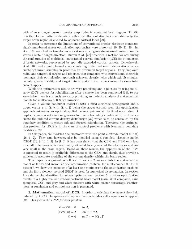
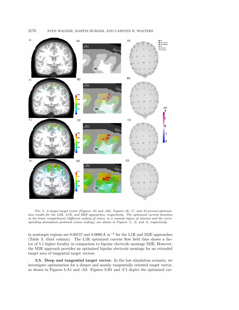
Fig. 5. A deeper target vector (Figures -A1 and -A2): Figures -B, -C, and -D present optimiza-tion results for the L2R, L1R, and M2E approaches, respectively. The optimized current densitiesin the brain compartment (different scaling of rows), in a zoomed region of interest and the corre-sponding stimulation protocols (same scaling), are shown in Figures -1, -2, and -3, respectively.

in nontarget regions are 0.00157 and 0.0080 A m−2 for the L1R and M2E approaches(Table 3, third column). The L1R optimized current flow field thus shows a fac-tor of 5.1 higher focality in comparison to bipolar electrode montage M2E. However,the M2E approach provides an optimized bipolar electrode montage for an extendedtarget area of tangential target vectors.

5.5. Deep and tangential target vector. In the last simulation scenario, weinvestigate optimization for a deeper and mainly tangentially oriented target vector,as shown in Figures 5-A1 and -A2. Figures 5-B1 and -C1 depict the optimized cur-


rent density distributions when using L2R and L1R for optimization, respectively.For those approaches, the target current densities are 0.015 and 0.019 A m−2, respec-tively. With a value of 0.052 A m−2, which is more than 2.7 times the L1R value,the largest target intensity is, however, achieved with the M2E approach (Table 3,second column). CDt values of 0.013, 0.018, and 0.049 A m−2 lead to PAR valuesof 86.7, 94.7, and 94.2 for the L2R, L1R, and M2E approaches (Table 3, fourth andfifth columns). The target current densities are thus for all three approaches orientedmainly parallel to the target vector.

The L2R and L1R stimulation protocols show high focality with mainly two activeelectrodes, while only weak compensating currents are injected at the neighboringelectrodes (Figures 2-B2 and -C2). Similar to section 5.2, the compensating currentsare stronger when using the L2R optimization procedure, leading to weaker targetbrain current densities as compared to the L1R stimulation. In order to enable currentdensity to penetrate into deeper brain regions, the distance between the two mainstimulating electrodes is larger when compared to the superficial mainly tangentialtarget vector from section 5.2; i.e., the electrode above the target region is not usedfor stimulation, while a more distant electrode is used as anode.

For all three approaches, strongest current density amplitudes in the brain com-partment always occur at the CSF/brain boundary above the target region (Figures5-B1, -C1, and -D1). This is due to the fact that the potential field ∇Φ satisfies themaximum principle for harmonic functions which states that a nonconstant functionalways attains its maximum at the boundary of the domain [15, Theorem 14.1]. Nev-ertheless, on average over all nontarget regions, with a value of 0.014 77 A m−2 forM2E, the L2R (0.003 45 A m−2) and L1R (0.002 49 A m−2) optimized current flowfields show a factor of about 4.3 and 5.9 times lower current densities, respectively(Table 3, third column). Overall, L2R and L1R thus have a much higher focality,which can also easily be seen in Figures 5-B1, -C1, and -D1. However, if no multi-channel tDCS device is available, the M2E approach provides an optimized bipolarelectrode arrangement for a deep and tangential target vector.

The deep target region does not seem to be located in a very deep region ofthe brain. It gets obvious that the deeper the target vector is located, the higherthe averaged maximal current density in the brain compartment, especially in morelateral brain regions. Due to the maximum principle it is thus not possible to targetdeep regions without stimulating more lateral brain areas. However, many importanttarget regions, e.g., auditory, motor, or visual cortex, are located rather laterally, sothat it will be possible to target with significant field strength in many applications.Moreover, in many applications of brain stimulation it might also not matter whethernontarget regions are also involved, because the experimental setup focuses on thetarget region, for example when examining the change in event-related potentials(ERPs) in pre- and post-tCS stimulation ERP measurements.

6. Conclusion and outlook. A novel optimization approach for safe and well-targeted multichannel t-DCS has been proposed. Existence of at least one minimizerhas been proven for the proposed optimization methods. For discretization of therespective minimization problems the FEM was employed and the existence of atleast one minimizer to the discretized optimization problems has been shown. For nu-merical solution of the corresponding discretized problem we employed the ADMM.A highly realistic six-compartment head model with white matter anisotropy wasgenerated, and optimized current density distributions were calculated and evaluatedfor a mainly tangential and a mainly radial target vector at superficial locations, an


extended target area, and a deeper mainly tangential target vector. The numericalresults revealed that, while all approaches fulfilled the patient safety constraint, theoptimized current flow fields show significantly higher focality and, with the exceptionof the L2R for the deep target, higher directional agreement to the target vector incomparison to standard bipolar electrode montages. The higher directional agree-ment is especially distinct for the radial target vector. In all test cases, because ofa more widespread distribution of injected and extracted surface currents, the L2Roptimization procedure (Pα,0

ε ) led to relatively weak current densities in the braincompartment. The L1R optimized current density distribution along the target direc-tion was in all test cases stronger than the L2R one and might thus be able to inducemore significant stimulation effects. The stimulation will thus enhance cortical ex-citability, especially in the target regions, while it will prevent too strong excitabilitychanges in nontarget regions as well as possible.

We were able to demonstrate that the M2E approach provides optimized bipolarelectrode montages as long as the target is mainly tangentially oriented. For radialtargets, the M2E approach was unsatisfactory; an optimal bipolar electrode configu-ration might then consist of a small electrode placed directly above the target regionwith a distant return electrode or a small electrode over the target encircled by a ringreturn electrode, as proposed in [10].

A further application for the optimization method is transcranial magnetic stim-ulation (TMS). TMS uses externally generated magnetic fields to induce electricalcurrents to the underlying brain tissue [16]. Because there is no safety limit for thetotal currents applied to the stimulating coils but a safety threshold for painful muscletwitching [16], the constrained optimization problem for multicoil TMS is given as

(PTMS) −∫

Ωt

〈σ∇Φ, e〉dx→ min

subject to ω|σ∇Φ| ≤ EM ,

∇ · σ∇Φ = −∇ · σ∂A(x, t)

∂tin Ω,

〈σ∇Φ,n〉 = −〈σ∂A(x, t)

∂t,n〉 on Γ,

Φ = 0 on ΓD

with A(x, t) being the time-dependent magnetic vector potential and EM = 450 V m−1

being the threshold for painful muscle twitching [16]. By designing the changes in the

magnetic vector potential one can consider ∂A(x,t)∂t as the optimization variables (re-

spectively, some parameters on which it depends linearly). The existence of at leastone minimizer to the constrained optimization problem for TMS directly follows witharguments similar to those in Theorem 3.2.

Because the optimization method can be applied for both brain stimulationmodalities, a combined tDCS and TMS optimization might outperform single modal-ity tDCS or TMS optimizations, similar to what was shown for electroencephalography(EEG) and magnetoencephalography (MEG) [4, 3]. While tCS is able to stimulatea radially oriented target, TMS is mainly not (like MEG is hardly able to detect ra-dial sources [4, 3]). Possible applications of combined tDCS and TMS multichanneland multicoil optimization might thus be an improved stimulation of target regionscontaining both radial and tangential orientations or of deeper target regions. In or-der to induce action potentials in deeper target regions, the induced current densityshould exceed the threshold for neuronal depolarization of 150 V m−1 [16]. On the


other hand, the threshold for painful muscle twitching of 450 V m−1 must be kept [16].The combination of the optimized tDCS and TMS current density fields might leadto higher current densities in the target and simultaneously reduced current densityamplitudes in nontarget regions.

While a thorough mathematical analysis of our novel multiarray tDCS optimiza-tion method was derived and results for different target regions were presented, be-sides the first promising results presented in [20], we did not yet further compare ourmethod to the existing approaches in the literature, such as, e.g., [10, 29, 21, 28].Such a comparison is one of our future research goals.

REFERENCES

[1] B. Agsten, Comparing the Complete and the Point Electrode Model for Combining tCS andEEG, Master thesis, University of Munster, Munster, Germany, 2015.

[2] B. Agsten, S. Wagner, S. Pursiainen, and C. H. Wolters, Advanced boundary electrodemodeling for tES and parallel tES/EEG, submitted.

[3] U. Aydin, J. Vorwerk, M. Dumpelmann, P. Kupper, H. Kugel, M. Heers, J. Wellmer,C. Kellinghaus, J. Haueisen, S. Rampp, H. Stefan, and C. H. Wolters, CombinedEEG/MEG can outperform single modality EEG or MEG source reconstruction in presur-gical epilepsy diagnosis, PLoS ONE, 10 (2015), e0118753.

[4] U. Aydin, J. Vorwerk, P. Kupper, M. Heers, H. Kugel, A. Galka, L. Hamid, J. Wellmer,C. Kellinghaus, J. S. Rampp, and C. H. Wolters, Combining EEG and MEG for thereconstruction of epileptic activity using a calibrated realistic volume conductor model,PLoS ONE, 9 (2015), e93154, https://doi.org/10.1371/journal.pone.0093154.

[5] L. J. Bindman, O. C. Lippold, and J. W. Redfearn, Long-lasting changes in the level of theelectrical activity of the cerebral cortex produced by polarizing currents, Nature, 10 (1962),pp. 584–585.

[6] P. S. Boggio, F. Bermpohl, A. O. Vergara, A. L. Muniz, F. H. Nahas, P. B. Leme,S. P. Rigonatti, and F. Fregni, Go-no-go task performance improvement after anodaltranscranial DC stimulation of the left dorsolateral prefrontal cortex in major depression,J. Affect. Disord., 101 (2007), pp. 91–98.

[7] S. Boyd, N. Parikh, E. Chu, B. Peleato, and J. Eckstein, Distributed optimization andstatistical learning via the alternating direction method of multipliers, Found. Trends Mach.Learn., 3 (2011), p. 1–122.

[8] O. D. Creutzfeldt, G. H. Fromm, and H. Kapp, Influence of transcranial d-c currents oncortical neuronal activity, Exp. Neurol., 5 (1962), pp.436–452.

[9] M. Dannhauer, D. Brooks, D. Tucker, and R. MacLeod, A pipeline for the simula-tion of transcranial direct current stimulation for realistic human head models usingSCIRun/BioMesh3D, in Proceedings of the Annual International Conference of the IEEEEngineering in Medicine and Biology Society, 2012; https://doi.org/10.1109/EMBC.2012.6347236.

[10] J. P. Dmochowski, A. Datta, M. Bikson, Y. Su, and L. C. Parra, Optimized multi-electrodestimulation increases focality and intensity at target, J. Neural Eng., 8 (2011), pp. 1–16.

[11] J. P. Dmochowski, A. Datta, Y. Huang, J. D. Richardson, M. Bikson, J. Fridriksson,and L. C. Parra, Targeted transcranial direct current stimulation for rehabilitation afterstroke, NeuroImage, 75 (2013), pp. 12–19.

[12] S. Eichelbaum, M. Dannhauer, M. Hlawitschka, D. Brooks, T. R. Knuesche, andG. Scheuermann, Visualizing simulated electrical fields from electroencephalography andtranscranial electric brain stimulation: A comparative evaluation, NeuroImage, 101 (2014),pp. 513–530.

[13] R. Ferrucci, F. Mameli, I. Guidi, S. Mrakic-Sposta, M. Vergari, S. Marceglia, F.Cogiamanian, S. Barbiere, E. Scarpini, and A. Priori, Transcranial direct currentstimulation improves recognition memory in Alzheimer disease, Neurology, 71 (2007), pp.493–498.

[14] F. Fregni, S. Thome-Souza, M. A. Nitsche, S. D. Freedman, K. D. Valente, and A.Pascual-Leone, A controlled clinical trial of cathodal DC polarization in patients withrefractory epilepsy, Epilepsia, 47 (2006), pp. 335–342.

[15] D. Gilbarg and N. S. Trudinger, Elliptic Partial Differential Equations of Second Order,Springer, Berlin, 2001.

https://doi.org/10.1371/journal.pone.0093154

https://doi.org/10.1109/EMBC.2012.6347236

https://doi.org/10.1109/EMBC.2012.6347236


[16] L. Gomez, F. Cajko, L. Hernandez-Garcia, A. Grbic, and E. Michielsson, Numericalanalysis and design of single-source multicoil TMS for deep and focused brain stimulation,IEEE Trans. Biomed. Eng., 60 (2013), pp. 2771–2782.

[17] R. F. Hartl, S. P. Sethi, and R. G. Vickson, A survey of the maximum principles foroptimal control problems with state constraints, SIAM Rev., 37 (1995), pp. 181–218, https://doi.org/10.1137/1037043.

[18] J. Haueisen, D. S. Tuch, C. Ramon, P. H. Schimpf, V. J. Wedeen, J. S. George, andJ. W. Bellveau, The influence of brain tissue anisotropy on human EEG and MEG,NeuroImage, 15 (2002), pp. 159–166.

[19] R. Herzog, G. Stadler, and G. Wachsmuth, Directional sparsity in optimal control ofpartial differential equations, SIAM J. Control Optim., 50 (2012), pp. 943–963, https://doi.org/10.1137/100815037.

[20] S. Homolle, Comparison of Optimization Approaches in High-Definition Transcranial CurrentStimulation in the Mammalian Brain, Master thesis, University of Munster, Munster,Germany, 2016.

[21] C. H. Im, H. H. Jung, J. D. Choi, S. Y. Lee, and K. Y. Jung, Determination of optimalelectrode positions for transcranial direct current stimulation (tDCS), Phys. Med. Biol.,53 (2008), pp. N219–N225.

[22] J.-L. Lions, Optimal Control of Systems Governed by Partial Differential Equations, Dunod,Gauthier-Villars, Paris, 1968.

[23] M. A. Nitsche, D. Liebetanz, A. Antal, N. Lang, F. Tergau, and W. Paulus, Modulationof cortical excitability by weak direct current stimulation–technical, safety and functionalaspects, Suppl. Clin. Neurophysiol., 56 (2003), pp. 255–276.

[24] M. A. Nitsche and W. Paulus, Excitability changes induced in the human motor cortex byweak transcranial direct current stimulation, J. Physiol., 527 (2000), pp. 633–639.

[25] C. Ortner and W. Wollner, A priori error estimates for optimal control problems withpointwise constraints on the gradient of the state, Numer. Math., 118 (2011), pp. 587–600.

[26] S. Pursiainen, F. Lucka, and C. H. Wolters, Complete electrode model in EEG: Rela-tionship and differences to the point electrode model, Phys. Med. Biol., 57 (2012), pp.999–1017.

[27] C. Ramon, P. Schimpf, J. Haueisen, M. Holmes, and A. Ishimaru, Role of soft bone, CSF,and gray matter in EEG simulations, Brain Topogr., 16 (2004), pp. 245–248.

[28] G. Ruffini, M. D. Fox, O. Ripolles, P. C. Miranda, and A. Pascual-Leone, Optimizationof multifocal transcranial current stimulation for weighted cortical pattern targeting fromrealistic modeling of electric fields, NeuroImage, 89 (2014), pp. 216–225.

[29] R. J. Sadleir, T. D. Vannorsdall, D. J. Schretlen, and B. Gordon, Target optimizationin transcranial direct current stimulation, Front. Psychiatry, 3 (2012), 90.

[30] A. Schiela and W. Wollner, Barrier methods for optimal control problems with convexnonlinear gradient state constraints, SIAM J. Optim., 21 (2011), pp. 269–286, https://doi.org/10.1137/080742154.

[31] D. S. Tuch, V. J. Wedeen, A. M. Dale, J. S. George, and J. W. Belliveau, Conductivitytensor mapping of the human brain using diffusion tensor MRI, Proc. Natl. Acad. Sci.USA, 98 (2001), pp. 11697–11701.

[32] S. Wagner, S. M. Rampersad, U. Aydin, J. Vorwerk, T. F. Oostendorp, T. Neuling,C. S. Herrmann, D. F. Stegeman, and C. H. Wolters, Investigation of tDCS volumeconduction effects in a highly realistic head model, J. Neural Eng., 11 (2014), 016002.

[33] W. Wollner, Optimal control of elliptic equations with pointwise constraints on the gradientof the state in nonsmooth polygonal domains, SIAM J. Control Optim., 50 (2012), pp.2117–2129, https://doi.org/10.1137/110836419.

https://doi.org/10.1137/1037043

https://doi.org/10.1137/1037043

https://doi.org/10.1137/100815037

https://doi.org/10.1137/100815037

https://doi.org/10.1137/080742154

https://doi.org/10.1137/080742154

https://doi.org/10.1137/110836419

an optimization approach for well-targeted transcranial...

Documents