an optimal control approach for scheduling mixed batch/continuous process plants with variable cycle...

Computers and Chemical Engineering 23 (1999) 907–917

An optimal control approach for scheduling mixedbatch/continuous process plants with variable cycle time

H.P. Nott 1, P.L. Lee *School of Engineering, Murdoch Uni6ersity, Perth WA 6150, Australia

Received 28 January 1998; received in revised form 18 March 1999; accepted 18 March 1999

Abstract

Effective scheduling of operations in the process industry has the potential to achieve high economic returns. Process plantscontaining both batch and continuous units present a difficult scheduling problem. When these processes are modelled with batchcycle times as decision variables, the complexity of the problem is increased significantly. These problems when modelled in theconventional MILP formulation are extremely difficult to solve as they are NP-hard. Many solution methods require unacceptableamounts of time/memory to solve even a simple problem. This paper considers an alternate way to represent the problem in anattempt to improve solution performance. This method is based on optimal control and the hierarchical splitting of theoptimisation problem. Results are compared to the traditional MILP formulation. The motivation for this work is an existingscheduling problem in the sugar milling industry. A smaller problem, which has characteristics of the sugar milling problem isconsidered for performance comparison. A substantial reduction in the complexity required to solve several test-cases of thisproblem is achieved using the optimal control formulation, while maintaining good quality solutions. © 1999 Elsevier Science Ltd.All rights reserved.

Keywords: Scheduling; Mixed integer programming; Mathematical modelling; Optimal control

1. Motivation

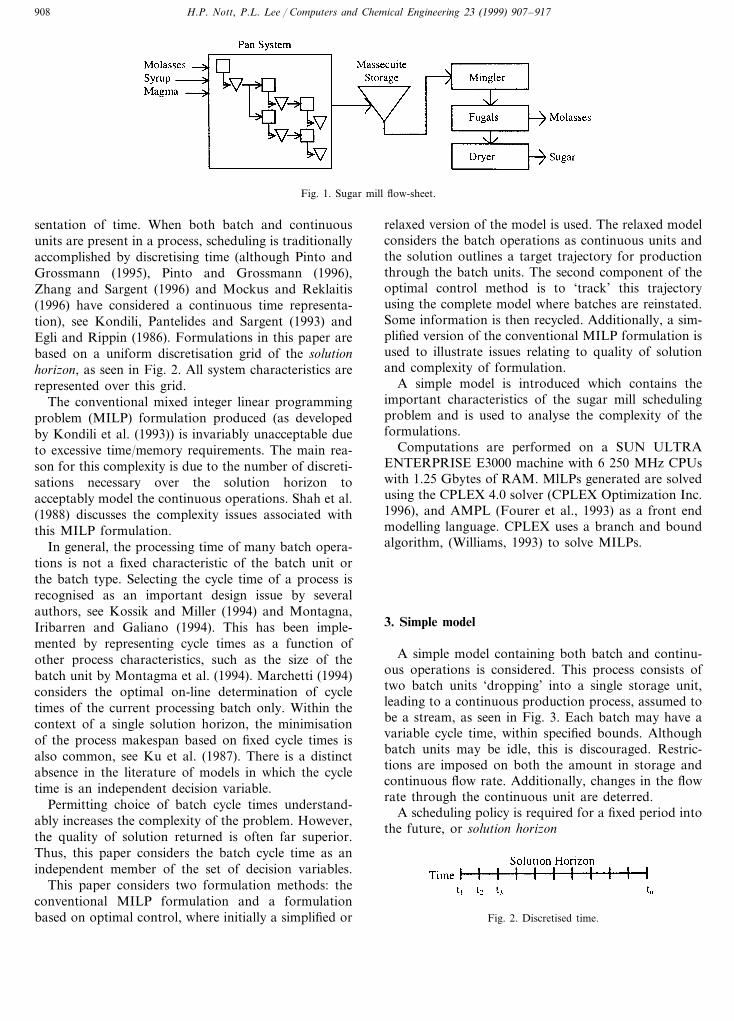
This study is motivated by the need for an optimalscheduling policy in sugar milling. Efficient schedulingof operations from crystallisation through to raw sugarproduction incorporating various batch (e.g. pans) andcontinuous units (e.g. fugals and dryers) has the poten-tial for high economic return. The system incorporatesnumerous process interactions as well as the sharing ofequipment between operations. Although the sugarmilling system shall not be considered in detail in thispaper, its general characteristics are the basis of thisstudy. Simply stated, the milling system consists of abatch pan system, followed by a communal, limitedstorage facility before the remainder of the downstreamprocess, which is generally considered to operate con-tinuously, as seen in Fig. 1.

The presence of both batch and continuous unitsmakes a difficult scheduling problem (Nott, 1998). Fur-thermore, although the batch units have a fixed quan-tity to process, each batch may take a variable length oftime to process. In this context, this is referred to ashaving variable cycle time. The physical system is con-strained by bounds on the cycle time of the batch pans,the limited storage facility as well as possible flow ratesthrough the continuous units.

A profit (turnover) is associated with the quantity ofsugar produced, while there is a cost incurred for theprocessing of each pan operation. It also is costly tohave a pan idle at any time and it is not advisable tomake drastic changes to the continuous flowrate, as thiscan seriously erode the performance of such units asdryers.

2. Introduction

Mockus and Reklaitis (1996) identify that one keyconsideration in any scheduling algorithm is the repre-

* Corresponding author.E-mail address: [email protected] (P.L. Lee)1 Present address: CSIRO Mathematical and Information Sciences,

Private Bag 10, South Clayton MDC, VIC 3169, Australia. E-mail:[email protected]

0098-1354/99/$ - see front matter © 1999 Elsevier Science Ltd. All rights reserved.

PII: S 0 0 9 8 -1354 (99 )00263 -X

H.P. Nott, P.L. Lee / Computers and Chemical Engineering 23 (1999) 907–917908

Fig. 1. Sugar mill flow-sheet.

sentation of time. When both batch and continuousunits are present in a process, scheduling is traditionallyaccomplished by discretising time (although Pinto andGrossmann (1995), Pinto and Grossmann (1996),Zhang and Sargent (1996) and Mockus and Reklaitis(1996) have considered a continuous time representa-tion), see Kondili, Pantelides and Sargent (1993) andEgli and Rippin (1986). Formulations in this paper arebased on a uniform discretisation grid of the solutionhorizon, as seen in Fig. 2. All system characteristics arerepresented over this grid.

The conventional mixed integer linear programmingproblem (MILP) formulation produced (as developedby Kondili et al. (1993)) is invariably unacceptable dueto excessive time/memory requirements. The main rea-son for this complexity is due to the number of discreti-sations necessary over the solution horizon toacceptably model the continuous operations. Shah et al.(1988) discusses the complexity issues associated withthis MILP formulation.

In general, the processing time of many batch opera-tions is not a fixed characteristic of the batch unit orthe batch type. Selecting the cycle time of a process isrecognised as an important design issue by severalauthors, see Kossik and Miller (1994) and Montagna,Iribarren and Galiano (1994). This has been imple-mented by representing cycle times as a function ofother process characteristics, such as the size of thebatch unit by Montagma et al. (1994). Marchetti (1994)considers the optimal on-line determination of cycletimes of the current processing batch only. Within thecontext of a single solution horizon, the minimisationof the process makespan based on fixed cycle times isalso common, see Ku et al. (1987). There is a distinctabsence in the literature of models in which the cycletime is an independent decision variable.

Permitting choice of batch cycle times understand-ably increases the complexity of the problem. However,the quality of solution returned is often far superior.Thus, this paper considers the batch cycle time as anindependent member of the set of decision variables.

This paper considers two formulation methods: theconventional MILP formulation and a formulationbased on optimal control, where initially a simplified or

relaxed version of the model is used. The relaxed modelconsiders the batch operations as continuous units andthe solution outlines a target trajectory for productionthrough the batch units. The second component of theoptimal control method is to ‘track’ this trajectoryusing the complete model where batches are reinstated.Some information is then recycled. Additionally, a sim-plified version of the conventional MILP formulation isused to illustrate issues relating to quality of solutionand complexity of formulation.

A simple model is introduced which contains theimportant characteristics of the sugar mill schedulingproblem and is used to analyse the complexity of theformulations.

Computations are performed on a SUN ULTRAENTERPRISE E3000 machine with 6 250 MHz CPUswith 1.25 Gbytes of RAM. MlLPs generated are solvedusing the CPLEX 4.0 solver (CPLEX Optimization Inc.1996), and AMPL (Fourer et al., 1993) as a front endmodelling language. CPLEX uses a branch and boundalgorithm, (Williams, 1993) to solve MILPs.

3. Simple model

A simple model containing both batch and continu-ous operations is considered. This process consists oftwo batch units ‘dropping’ into a single storage unit,leading to a continuous production process, assumed tobe a stream, as seen in Fig. 3. Each batch may have avariable cycle time, within specified bounds. Althoughbatch units may be idle, this is discouraged. Restric-tions are imposed on both the amount in storage andcontinuous flow rate. Additionally, changes in the flowrate through the continuous unit are deterred.

A scheduling policy is required for a fixed period intothe future, or solution horizon

Fig. 2. Discretised time.

H.P. Nott, P.L. Lee / Computers and Chemical Engineering 23 (1999) 907–917 909

Fig. 3. Simple batch-continuous model.

uniform discretisation solution horizon (as shown inFig. 2). Thus, at each time unit it is necessary todetermine:1. Does a batch start?2. Does a batch finish?3. What is the flowrate through the continuous unit?4. What is the implied amount in storage?Additionally, idle periods, or ‘batches’ are of unitlength. This is best illustrated by the batch operatingdecision variables:

if batch unit u begins a batch at time t orWut=1unit u is idle,0 otherwise.if batch unit u is processing a batch at time tYut=10 otherwise.

Batch operations represented by variable combinationsgiven in Table 1.

Behaviour of the continuous unit are given by:

X, the flow through the continuous unit from time t totime t+1.

The remaining variables assist model clarity:

But=1 if batch unit u begins a batch at time t,0 otherwise.

Eut=1 if batch unit u ends a batch at time t,0 otherwise.

Cut (integer) the number of batches and unit idleperiods from time T0 to time t

St the implied amount in storage at time t.cumulative production from time T0 to time tPRt

Recall the objective is to

maximise: turnover−batch costs− idle penalty

−flow penalty

In the conventional MILP formulation this is repre-sented by:

Turnover=sell�PRTF

Batch costs= %u�Ut�T

costu�Bu,t

Maximise: turn over−batch costs− idle penalty

−flow penalty

turnover for productionturnoverwherethrough the system

batch costs costs associated with begin-ning a batch

idle penalty penalty for scheduling idlebatch units

flow penalty penalty for changes in thecontinuous flowrate

The general nomenclature is given by:

num–units number of batch unitsTO start of the solution horizonTF end of the solution horizonset U= domain of batch units

num 6 unitsset T= the solution horizon

T0 … TFZu size of each batch for batch unit u in

UminPu minimum cycle time for batch unit u

in UmaxPu maximum cycle times for batch unit u

in UminX minimum flowrate through the con-

tinuous unitmaxX maximum flowrate through the con-

tinuous unitminS storage minimum at any timemaxS storage maximum at any timeS0 initial amount in the storage facility

turn-over/unit producedsellcostu cost price per batch begun on batch

unit u in Upenalty for idle periodspenI

penX flow rate changes penalty

4. Conventional MILP formulation

The conventional MILP formulation is based ondetermining individual solution choices for each com-ponent of the system at every time interval of the

Table 1Operation of a batch unit

YutWut Operation

1 1 Begin a batchContinue a batch10

01 Unit is idle0 1 Infeasible


Fig. 4. Dynamic model.

Fig. 6. Optimising the relaxed model.

Idle penalty=penI� %u�Ut�T

(1−Yu,t)

Flow penalty= %t�T:t\T0

penX��Xt−Xt−1�

It is necessary to incorporate a large number ofBoolean relationships/constraints (involving binaryvariables) in the conventional MILP formulation toensure feasibility, as shown in Appendix A. Refer toNott and Lee (1999) for an in-depth explanation on thisformulation.

5. Applying optimal control to scheduling

It has been found that optimal control can be auseful modelling tool for complex scheduling problems(Kogan & Khmelnitsky, 1996). The optimal controlproblem is expressed as: to find among all the accept-able control functions u, the one which minimises theperformance criteria J, subject to the dynamic systemconstraints and all initial and final boundaryconditions.

In discrete time, the dynamic systems are described interms of state variables x(t) by:

x(k+1)= f(x(k), u(k))

The state and control variables may both be con-strained. The most general performance criterion is:

J=F(x(N))+ %N−1

k=0

L(x(k), u(k)) for discrete time

Fig. 4 shows the relationship between control vectors, uand state vectors, x for model P. Often the stateequations of model P are very complex, and the modelis simplified or relaxed to P0. This incurs a modellingerror of DP as is shown in Fig. 5.

Optimal control has been applied to scheduling by ahierarchical splitting of the optimisation problem intotwo components (Kogan & Khmelnitsky, 1996). Thefirst step involves determining an optimal trajectory for

the relaxed model, P0. This is shown in Fig. 6. In asubsequent second stage, the full process model, P isforced to ‘track’ this optimal trajectory. The success ofthis method clearly depends on how close the optimaltrajectory, X0* (from the relaxed model, P0) approxi-mates the true optimum. X* (which would result froma direct optimisation of the complete model P).

To reduce the effect of modelling error a closed-loopor feedback control may be applied. A controller Ctakes corrective action when a tracking error. X0*−Xis detected, as also shown in Fig. 7.

Kogan and Khmelnitsky (1996) identified that themethodology behind optimal control can be a helpfulinstrument in solving scheduling problems, by using arelaxed model to produce a reference trajectory that isthen tracked. This is implemented in this paper by anoff-line method, which attempts to track the referencetrajectory with the complete model as a means toreduce the complexity required to find an optimalschedule for the defined solution horizon (Brandimarte,Ukovich & Villa, 1995, Kim & Leachman, 1993). Opti-mal control has also been applied in an on-line ordynamic nature, where the trajectory in tracked whileincorporating real scheduling changes as they occur(Brandimarte et al., 1995).

6. Optimal control implementation

The optimal control algorithm discussed in this papermaintains a discrete time representation (with similarstructure to the traditional MILP formulation) and isimplemented with some feedback information, or cor-rective control.

Fig. 7. Corrective control by feed-back loop.Fig. 5. Relaxed model and modelling error.


Fig. 8. Relaxed model: batch units as continuous operations.

where

Öt�T :minX5Xt5maxX Öt�T :minS5St5maxS

Öt�T :PRt]0 Öu�U, Öt�T :Fu,t, PRUu,t,Nu,t

Constraints of the system are:� No batches are already processing at the beginning

of the solution horizon:

Fut=0 Öu, Öt :t5minPu

� The flowrate through the ‘batch’ units is restrictedby batch size:

�tt� t...min(t+minPu−1, TF)Fu,tt5Bu,t Öu, Öt\T0� Update ‘batch’ cumulative production:

initially PRUu,Tbegin=Fu,T0

Öuthen PRUu,t=PRUu,t−1+Fu,t Öu, Öt\T0� Define the number of ‘batches’ by the ‘batch’ cumu-

lative final production:

PRUu,TF=Nu�Bu Öu� Maximum number of ‘batches’ over the solution

horizon:Nu5 (TF−T0)/minPu Öu� Update storage:

initially ST0=S0then St=St−1−Xt−1+�u Fu,t

Öt\T0� Feasible storage:

St−Xt]minS Öt� Update system production:

initially PRT0=0then PRT=PTt−1+Xt−1 Öt

Recall the overall objective is to:maximise: turnover−batch costs− idle penalty

−flow penaltv

In the relaxed model these are represented by:� Turnover for the entire solution horizon +

{sell*PRTF}� Batchcosts are calculated by the total production

through each batch unit over the solution horizonand the size of each batch on the associated unit:

−!�u costu�Nu

"� Idle penalty only incurred for forced idle periods,

based on the final production level through thesystem and the maximum cycle time:

−!

penI� if {TF−T0\Nu�minPu−1} then �u TF−T0−Nu�min Pu+1"

� Flow penalty for changes in the flowrate through the

continuous unit:−!�t\T0 penX��Xt−Xt−1�"

As the only objective component not fully accountedfor is the idle penalty the relaxed model should closelyapproximate the complete model—even though the

The optimal control algorithm is represented by:1. Use a relaxed representation of the model to pro-

duce some reference trajectory.2. Apply corrective control by modifying the reference

trajectory to reduce the effect of states that areknown to be undesirable.

3. Track the modified reference trajectory using thecomplete model.

4. If the solution schedules an undesired state repeatthe process by considering: the reference trajectoryas the complete solution just found. And return tostep 2.

This is repeated until some cyclic information isreturned (revisiting a previous solution space), or noundesired states scheduled.

Undesirable states in this context are periods ofidleness on the batch units.

Firstly the relaxed model and reference trajectory forthe problem considered in this paper shall be discussed(step 1). Following this corrective control measures areconsidered (step 2) and finally methods to track thereference trajectory are given (step 3).

7. The relaxed model and reference trajectory

Optimal control has most popularly been applied tomanufacturing scheduling (Brandimarte et al., 1995)and this commonly involves a continuous flow modelrepresentation of discrete decisions. As Nott (1998) hasshown, the presence of both batch and continuous unitsconstitutes a significant proportion of the schedulingcomplexity, and hence to simplify this problem, batchunits are represented as continuous operations as seenin Fig. 8.

The decision variables for the relaxed model are:

Fu,t the flowrate through the ‘batch’ unit u at timet

Xt the flowrate through the continuous unit attime t

as well as the auxiliary variables:

PRUut the cumulative production through ‘batch’unit u at time t

Nu the number of ‘batches’ begun on unit uthe amount in the storage facility at time tSt

PRt the cumulative production of the system upto time t


Fig. 9. Determining influence of cycle times by rounding the reference trajectory.

cumulative production curve between the relaxedmodel and the complete model appear different (con-tinuous vs. step structure). Furthermore, methods todeter idle periods are considered in the next section.

8. Corrective control procedures–generating modifiedtrajectories

The optimal control implementation is based ontracking the reference trajectory obtained by the re-laxed version of the model (see Section 7). However,firstly some corrective control procedures are appliedwhich may modify the reference trajectory. The pur-pose of these procedures is to reduce the risk of un-desirable states in the reference trajectory, prior tothe complete model tracking this curve (discussed inthe next section). If the reference trajectory incorpo-rates an undesirable state, the complete model willalso be inclined to incorporate the same undesirablestate. Generally, these undesirable states are statesthat were not fully represented in the relaxed model.

For the system being considered, the scheduling ofidle periods on the batch units is undesirable. More-over, this is also the only objective function compo-nent that was not fully represented in the relaxedmodel (Section 7). After optimising the relaxed modelto obtain the reference trajectory, idle periods caneasily be identified using maximum cycle time infor-mation. This section presents methods to manipulatethe reference trajectory to reduce any tendency to-wards scheduling idle periods while maintaining theoverall shape of the reference trajectory (or produc-tion through the ‘batch’ units).

The favoured batch cycle times are given by round-ing the cumulative production reference trajectory tothe closest multiple of batch cycle time, or roundedtrajectory. Fig. 9 shows how the rounded trajectory is

used to indicate preferred cycle times (and batch com-pletion times). When there is a longer than maximumcycle time length of time between batch completions(steps in the cumulative production), a preference toschedule an undesirable idle period is indicated. Forthis purpose a block is identified by constant cumula-tive production, containing a batch and perhaps idleperiods.

Suppose the batch unit whose production is shownin Fig. 9 has a maximum cycle time of six units. Onebatch completes at time=4 and the next does notcomplete until time=12. This is two time unitslonger than the maximum cycle time and is thus con-sidered an offending block. That is, as cumulative pro-duction remains constant for a period of time longerthan the maximum cycle time, this must contain botha batch and periods of idleness.

The reference trajectory is modified by shorteningthe offending block and is implemented in one of twoways:1. The preferred method is to lengthen the batch prior

to the offending batch, if its cycle time is less thanthe maximum. This shortens the offending block bystarting it later and is seen in Fig. 10 where thereference trajectory is lowered at the start of theoffending block (time=4).

2. The alternate is to start all batches (or blocks)following the offending block earlier, thus stillmaintaining the cycle time characteristics of thesebatches. This shortens the offending block by finish-ing it earlier and is seen in Fig. 10 where thereference trajectory is raised at the completion of allfollowing blocks (time=11, time=13 and time=19).

Both procedures are consistent with the major objectivecomponent of the problem to maximise overall produc-tion of the system.


Fig. 10. Reducing influence of reference trajectory for idle periods. Fig. 11. Tracking the reference trajectory.

X, the flowrate through the continuous unit at time t

As well as the binary variables:

Eu,t

=1 if a batch ends on unit u at time t, or 0 otherwise

In addition, there are auxiliary variables:

PRUu,t integer, cumulative production through‘batch’ unit u at time t

St the amount in the storage facility at time tPRt the cumulative production of the system up

to time t

with bounds

Öt�T :minX5Xt5maxX Öt�T :minS5St5maxS

Öt�T :PRt]0

Öu�U, Öt�T :Eu,t�{0, 1}, PRUu,t�Z

The objective of the complete model involves minimis-ing the difference between the tracking curve and theactual curve produced as seen in Fig. 11, being consis-tent with the common optimal control performancecriteria, J : to minimise the square of the differencebetween the curves (as seen in Fig. 11). Time remainsdiscretised and a MILP formulation is produced. Thusthe complete model considers the reference trajectory asa parameter specification:

Tut reference trajectory as given by the relaxed model in stage 1

and deviations from the reference trajectory are pe-nalised by penT

Furthermore, the overall objective of this stage of theoptimal control approach is completely described bythe non-batch components of the complete model aswell as tracking the reference trajectory. The objectiveis to:

maximise: turnover− tracking penalty−flow penalty

These corrective control procedures are appliedwhenever a new reference trajectory is produced. If thesolution from the complete model (as will be discussedin Section 9) schedules an idle period, this solution isconsidered the new reference trajectory and correctivecontrol procedures are applied to eliminate any prefer-ence to schedule idle periods. This is repeated untileither no idle periods are schedule (when solving withthe complete model) or some cyclic behaviour isidentified.

9. Tracking the reference trajectory using the completemodel

Once the cumulative batch production reference tra-jectory has been attained using the relaxed model, thiscurve is then considered as a whole and no longer asindividual decisions at each point in time. Once anymodifications have been performed, the objective is totrack this using the complete model with batch opera-tions reinstated.

The ‘complete’ model used in step 3 of the optimalcontrol implementation is considerably simpler than theoriginal conventional MILP formulation as the batchcomponent of the complete model may be fully repre-sented by the completion of batch operations. Morespecifically, the starting times of batches do not need tobe explicitly identified in this stage of the optimalcontrol implementation. Firstly, it is possible to omitbatch starts as no other components of the mixed-batch/continuous system being considered are depen-dent on the start time of these operations, as seen inFig. 3. Secondly, the sole purpose of including batchstarts in the system would be for identifying idle peri-ods. The multi-stage nature of the optimal controlapproach enables idle periods to be implicitly identifiedand deterred by corrective control procedures as dis-cussed in the previous section.

The system variables for the complete model are:


where

turnover= +{sell�PRTF}

tracking penalty= −!

penT�%u,t

�PRUu,t−Tu,t �"The constraints of the complete model are:� Restrictions for the initial batch:

PRUu,t=0 Öu, Öt5minPuEu,t=0 Öu, Öt5minPu

� Batch unit production:PRUu,t=PRUu,t−1+Eu,t�Zu Öu, Öt\minP

� Batches must be at least minimum cycle time:�Eu,tt51

tt� t...min(t+minPu−1,TF)Öu, Öt

� Update storage:initially ST0=S0then PRT0=0

� Feasible storage:St−Xt]minS Öt

� Update system production:initially PRT0

then PRt=PRt−1+Xt−1 Öt

10. Discussion on model quality

One concern associated with the quality of the optimalcontrol solution is related to the model formulation notexplicitly allowing for idle periods. A simplified versionof the conventional MILP formulation is given in theappendix. This does not have idle periods explicitlyrepresented, resulting in a much simpler formulation,which appears relatively similar to the optimal controlimplementation.

However, the optimal control approach is able toproduce solutions of high quality—comparable to thetraditional MILP formulation, which the simplifiedMILP is unable to produce due to its hierarchical nature.

11. Results

The quality of solution can easily be assessed, as theconventional MILP formulation is guaranteed to returnthe true optimal solution, or X*. Following the optimal

control terminology, the solution produced by the opti-mal control implementation is X which attempts to trackthe reference trajectory X0* given by the relaxed model.

Table 2 displays several different problem specifica-tions. The solution quality and performance of theseproblems is given in Table 3. This shows that the timerequired to solve the optimal control implementation isdramatically less than the traditional MILP approach.Problem 1 in Table 3 does not require the considerationof idle scheduling and thus both the optimal controlapproach and the simplified MILP return the optimalsolution in excellent time. However, the solution returnedfrom the optimal control approach—while not guaran-teed to be optimal, is much more reliable that thesimplified MILP—as is shown to be the case in problem5, where the simplified MILP fails to return the optimalsolution. The quality of the simplified MILP solution inproblem 6 is even worse, while the optimal controlapproach returns a reasonably good solution.

The solution to problem 1 is given for the traditionalMILP formulation and the optimal control method aregiven in Table 4 and Table 5, respectively. Rounding the‘batch’ production given by the optimal control relaxedmodel to the nearest multiple of batch size did not yieldany offending blocks and hence, no corrective controlprocedures were required before using the completemodel to track this trajectory.

12. Conclusions

The optimal control approach presented in this paperhas excellent performance for a problem that has beenshown to be very difficult to solve. While the solutionproduced is not guaranteed to be optimal, a high qualitysolution is able to be returned.

Appendix A

A.1. Traditional MILP formulation

A.1.1. Variables

Wu,t, Yu,t, Bu,t, Eu,t�{0, 1} Öu�U, Öt�T

Table 2Problem specifications—solution and performance results (always T=1�25, wXdev= l, cost–idle=100, sellprice=20)

Num–units Min P Max P Min X Max X Min S Max S S0B Cost

2 8, 10 3, 4Problem 1 60, 505, 6 101525.02.53, 410,102Problem 2 1015 60, 5025.02.53, 4

3 10, 10, 10 3, 4, 2 5, 6 2.5Problem 3 10.0 2 20 10 60, 50, 40Problem 4 10, 10, 103 60, 50, 40102027.52.55, 6, 63, 4, 4

8, 10 3, 4 5, 6, 6 2.5Problem 5 5.02 2 15 10 60,508, 10 2, 3 4, 5 2.5 5.0 2 15Problem 6 102 60, 50

60, 50202044.02.52 5, 5Problem 7 2, 38,10


Table 3Solution and performance results

Optimal control MeasureTraditional MILP Simplified MILP

1 iteration 2 iterations

1415.08 Solution1415.08Problem 1 1415.08User time4:26.3 0.4 0.5

1537.7Problem 2 1537.7 1537.7 Solution0.5 User time0.323.0

SolutionProblem 3 3314 3314 3314User time0.61.012.29

2340.3Problem 4 2340.2 2340.2 Solution0.750:28.6 0.8 User time

Solution1415.081388.5Problem 5 1415.08User time1:04.2 5:44.5 0.5Solution1078.42−1001.5Problem 6 1188.5

3.815:45.3 5.3 User time820 1320Problem 7 1320 1320 Solution

User time1.20.75:092.0

Cut integerÖu�U, Öt�T

minX5Xt5maxX Öt�T

minS5St5maxS Öt�T

PRt]0 Öt�T

A.1.2. Objecti6e function

Max sell�PRTF− %u�Ut�T

costu�Bu,t−penI� %u�Ut�T

(1−Yu,t)

− %t�T:t\0


A.1.3. Constraints

At the beginning of the solution horizon, T0� each batch unit, u is processing a batch, or is idle:

Cu,T0=0 Öu�U� no batches have completed processing on any unit,

u : Eu,T0=0 Öu�U� the amount in storage is initialised: ST0=S0

� and production through the system is initialised:PRT0=0At any time, t, if a batch starts on a batch unit, u, or

the unit is idle, a counter is incremented:

Cu,t=Cu,t−1+Wu,t Öu�U, Öt�T :t\T0

Batch cycle times must be longer than the specifiedminimum for that unit:

Cu,tt−Cu,t5 (TF−T0)�(1−Bu,t) Öu�U, Öt�T,

Ött� (t+1)...min(t+minPu−1, TF)

Batch cycle times must be shorter than the specifiedmaximum for that unit, u :

Cu,t−Cu,t−maxPu]1 Öu�U, Öt�T :t]T0+max Pu

An idle period at any time t, on any ‘batch unit’ u mustbe of unit length and associated feasibility relationships:

Wt,u+Yu,t]1 Öu�U, Öt�T

Yu,t−1−Wu,t5Yu,t5Yu,t−1+Wu,t Öu�U,

Öt�T :t\T0

Table 4Traditional MILP solution

T XW1 PRW2 S

2.667101 0110 7.333 2.667 2.6672 0

3 5.3332.6674.66700510 80144.875 135 0 1 15

17.8754.87510.1256 001 22.757 4.87513.250

27.6250 0 8.375 4.87584.87513.5 32.59 10

0 8.62510 4.875 37.375042.254.87501 11.751147.1250 4.87512 6.8750

0 113 12 5254.333 5714 1 0 154.333 61.33315 0 0 10.667

65.6674.3336.33316 00101 5 70017

18 7551510510 800019520 851 0 13

0 021 8 5 9022 0 1 13 5 95

10058023 01 024 11 5 105025 0 6 4 110


Table 5Optimal control solution

Rounded Complete modelRelaxed

E2 PRXT SPRU1 PRU2 T1 T2 PRU1 PRU2 E1

0 10 2.6671 0 0 0 0 0 0 000 2.6672.6672 0 0 0 7.3330 0 0 0

0 4.667 2.6673 0 5.3330 0 0 0 0 0

510 84 6 0 08 0 8 0 11 15 4.8755 6 3.6 8 0 138 10 0

17.874.87510.126 8 10 08 10 8 10 00 13.25 4.8757 14 22.7510 16 10 16 10 1

4.875 27.628 14 8.37510 016 10 16 10 01 13.5 4.8759 16 32.513.6 16 10 16 20 0

37.374.8758.62510 22 20 024 20 16 20 00 11.75 4.87511 22 42.2520 24 20 24 20 1

4.875 47.1212 24 6.87520 024 20 24 20 01 12 513 30 23.6 32 20 24 5230 0

574.3331514 30 30 032 30 32 30 10 10.66 4.33315 30 61.3330 32 30 32 30 0

4.333 65.6616 36 6.33330 032 30 32 30 00 10 517 36 7033 32 30 40 30 1

7551518 38 40 140 40 40 40 00 10 519 44 8040 48 40 40 40 0

8551320 44 40 048 40 48 40 10 8 521 46 43 9048 40 48 40 0

9551322 46 50 148 50 48 50 00 8 523 49 10050 48 50 48 50 0

5 10524 54 1150 056 50 56 50 10 6 425 54 52.5 11056 50 56 50 0

The beginning of a batch on unit u at time t is definedby Bu,t and given by:

Wu,t+Yu,t−15Bu,t5 (Wu,t+Yu,t)/2 Öu�U, Öt�T

The completion of a batch on unit u at time t is definedby Eu,t and given by:

Wu,t+Yu,t−1−15Eu,t5 (Wu,t+Yu,t−1)/2 Öu�U,

Öt�T :t\T0

Storage levels must even be feasible within (as well asat) each time unit, t :

St−Xt]minS Öt�T

Storage is updated at each time unit, t :

St=St−1−Xt−1+ %u�U

Eu,t�Zu Öt�T :t\T0

Production is updated at each time unit, t :

PRt=PRt−1+Xt−1 Öt�T

Simplified MILP formulation

A.1.4. Variables

Eu,t�{0, 1} Öu�U, Öt�T

Cut integer Öu�U, Öt�T

minX5Xt5maxX Öt�T

minS5St5maxS Öt�T

PRt]0 Öt�T

A.1.5. Objecti6e

Maximise: sell�PRTF− %u�Ut�T

costu�Bu,t

−penI� %u�U

max(CuTF�max Pu−1−TF+T0, 0)

− %t�T:t\T0


A.1.6. Constraints

At T0: Cu,T0=1 Öu�U ; Eu,T0=0 Öu�U ;

ST0=S0; PRT0=0

At any time, t, if a batch starts on a batch unit, u, orthe unit is idle, a counter is incremented:

Cu,t=Cu,t−1+Eu,t Öu�U Öt�T :t\T0


Batch cycle times must be longer than the specifiedminimum for that unit:

Cu,tt−Cu,t5 Öu�U, Öt�T,

Ött� t ... min(t+minPu−1, TF)

Storage levels must even be feasible within (as well asat) each time unit, t : St−Xt]min S Öt�TStorage isupdated at each time unit, t :

St=St−1−Xt−1+ %u�U

Eu,t�Zu Öt�T :t\T0

Production is updated at each time unit t :

PRt=PRt−1+Xt−1 Öt�T

References

Brandimarte, P., Ukovich, W., & Villa, A. (1995). Continuous flowmodels for batch manufacturing: a basis for a hierarchical ap-proach. International Journal of Product Research, 33(6), 1635–1660.

CPLEX Optimization Inc. (1996). Users manual, Nevada, USA.Egli, U. M., & Rippin, D. W. T. (1986). Short-term scheduling for

multiproduct batch chemical plants. Computers & Chemical Engi-neering, 10(4), 303–325.

Fourer, R., Gay, D. M., & Kernighan, B. W. (1993). AMPL: amodelling language for mathematical programming. Massachusetts:Boyd and Fraser.

Kim, S.-Y., & Leachman, R. C. (1993). Multi-project scheduling withexplicit lateness costs. IIE Transactions, 25(2), 34–44.

Kogan, K., & Khmelnitsky, E. (1996). an optimal control model forcontinuous time production and setup scheduling. InternationalJournal of Production Research, 34(3), 715–725.

Kondili, E.., Pantelides, C. C., & Sargent, R. W. T. (1993). A generalalgorithm for short-term scheduling of batch operations—I. MILPformulation. Computers & Chemical Engineering, 17(2), 211–227.

Kossik, J. M., & Miller, G. (1994). Optimize cycle times for batchbiokill systems. Chemical Engineering Progress, 90(10), 45–51.

Ku, H.-M., Rajagopalan, D., & Karami, I. (1987). Scheduling in batchprocesses. CEP, 83, 35–54.

Marchetti, J. L. (1994). Optimal cycle time in semi-batch ultrafiltrationsystems. Chemical Engineering Communications, 129, 217–225.

Montagna, J. M., Iribarren, O. A., & Galiano, F. C. (1994). The designof multiproduct batch plants with process performance models.Chemical Engineering Research & Design, 72(A6), 783–791.

Mockus, L., & Reklaitis, G. V. (1996). A continuous time representa-tion in batch/semicontinuous process scheduling: randomizedheuristics approach. Computers & Chemical Engineering, 520,S1173–S1177.

Montagma, J. M., Iribarren, O. A., & Galiano, F. C. (1994). The designof multiproduct batch plants with process performance models.Chemical Engineering Research and Design, 72(A6), 783–791.

Nott H. P. (1998). Modelling alternatives for scheduling mixed batch/continuous process plants with variable cycle time. PhD Thesis,Murdoch University, Western Australia.

Nott H. P. & Lee P. L. (1999). Sets formulation to schedule mixedbatch/continuous process plants with variable cycle time. Comput-ers & Chemical Engineering (in press)

Pinto, J. M, & Grossmann, I. E. (1995). A continuous time mixedinteger linear programming model for short term scheduling ofmultistage batch plans. Industrial Engineering Chemical Research,34, 3037–3051.

Pinto, J. M., & Grossmann, I. E. (1996). A continuous time MILPmodel for short term scheduling of batch plants with pre-orderingconstraints. Computers & Chemical Engineering (supp), 20, S1197–S1202.

Shah, N., Pantelides, C. C., & Sargent, R. W. H. (1993). A generalalgorithm for short-term scheduling of batch operations—II Com-putational issues. Computers and Chemical Engineering, 17(2),229–244.

Williams, H. P. (1993). Model building in mathematical programming.England: Wiley.

Zhang, X., & Sargent, R. W. H. (1996). The optimal operation of mixedproduction facilities—a general formulation and some approachesfor the solution. Computers & Chemical Engineering, 20(6/7),897–904.

.

an optimal control approach for scheduling mixed batch/continuous process plants with variable cycle...

Documents