1

An Optimal Confidence Region for for the Best and the Worst Populations

Speaker: Prof. Hubert J. Chen, Institute of Finance National Cheng Kung U., Taiwan

2012.11.21 Invited Talk at Dept. of Statistics, Ping-Tung Edu. U.

Jointly with: Prof. Shu-Fei Wu, Tamkang U., Taiwan

2

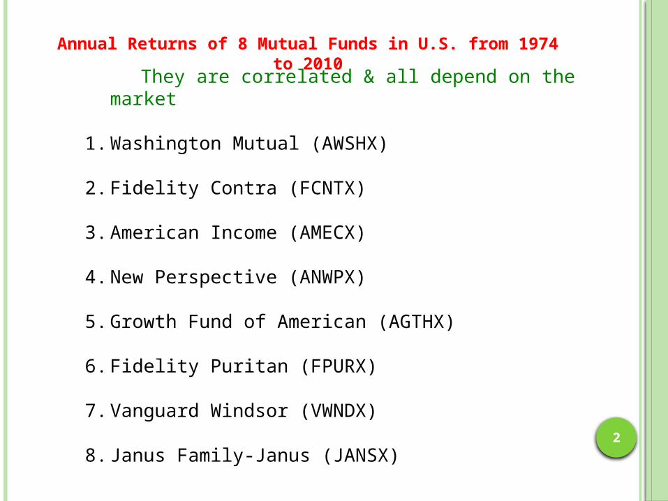
They are correlated & all depend on the market

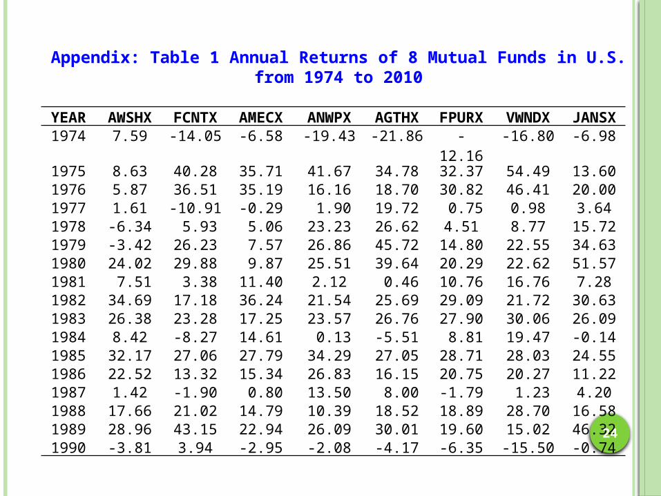
1. Washington Mutual (AWSHX)

2. Fidelity Contra (FCNTX)

3. American Income (AMECX)

4. New Perspective (ANWPX)

5. Growth Fund of American (AGTHX)

6. Fidelity Puritan (FPURX)

7. Vanguard Windsor (VWNDX)

8. Janus Family-Janus (JANSX)

Annual Returns of 8 Mutual Funds in U.S. from 1974 to 2010

3

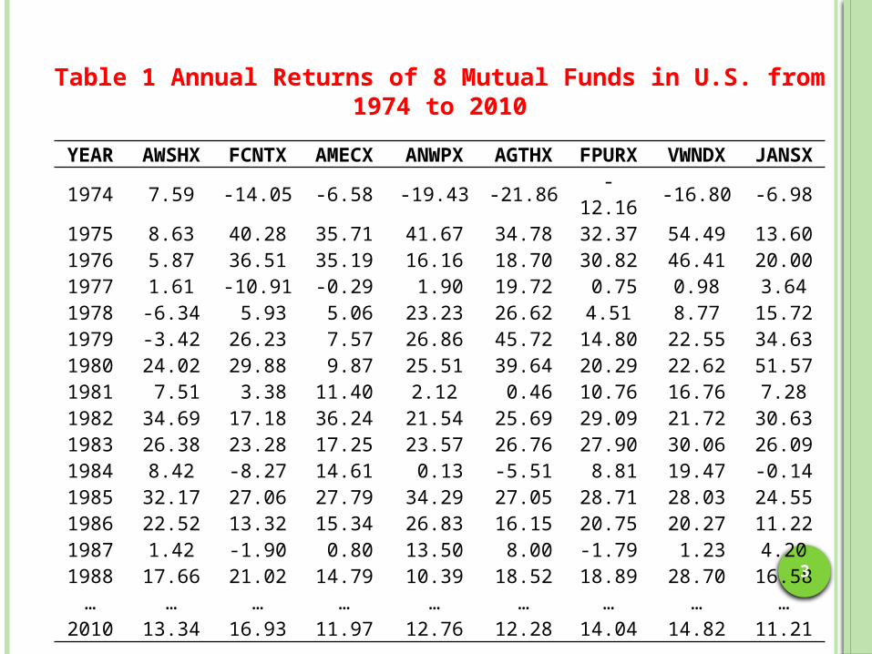
YEAR AWSHX FCNTX AMECX ANWPX AGTHX FPURX VWNDX JANSX1974 7.59 -14.05 -6.58 -19.43 -21.86 -12.16 -16.80 -6.981975 8.63 40.28 35.71 41.67 34.78 32.37 54.49 13.601976 5.87 36.51 35.19 16.16 18.70 30.82 46.41 20.001977 1.61 -10.91 -0.29 1.90 19.72 0.75 0.98 3.641978 -6.34 5.93 5.06 23.23 26.62 4.51 8.77 15.721979 -3.42 26.23 7.57 26.86 45.72 14.80 22.55 34.631980 24.02 29.88 9.87 25.51 39.64 20.29 22.62 51.571981 7.51 3.38 11.40 2.12 0.46 10.76 16.76 7.281982 34.69 17.18 36.24 21.54 25.69 29.09 21.72 30.631983 26.38 23.28 17.25 23.57 26.76 27.90 30.06 26.091984 8.42 -8.27 14.61 0.13 -5.51 8.81 19.47 -0.141985 32.17 27.06 27.79 34.29 27.05 28.71 28.03 24.551986 22.52 13.32 15.34 26.83 16.15 20.75 20.27 11.221987 1.42 -1.90 0.80 13.50 8.00 -1.79 1.23 4.201988 17.66 21.02 14.79 10.39 18.52 18.89 28.70 16.58… … … … … … … … …

2010 13.34 16.93 11.97 12.76 12.28 14.04 14.82 11.21

Table 1 Annual Returns of 8 Mutual Funds in U.S. from 1974 to 2010

4

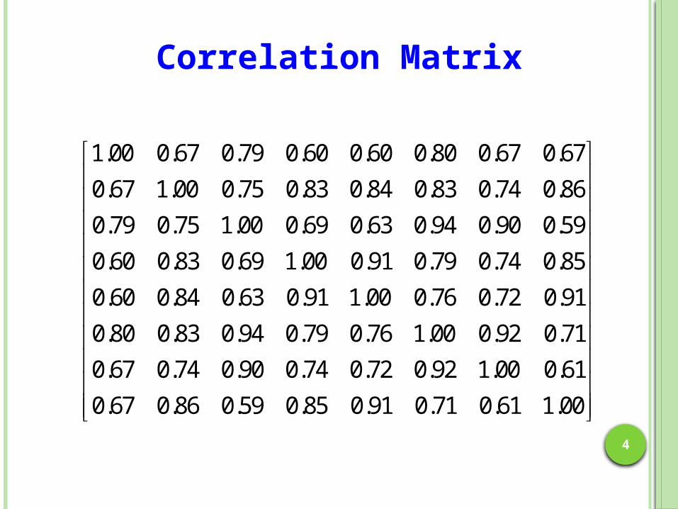
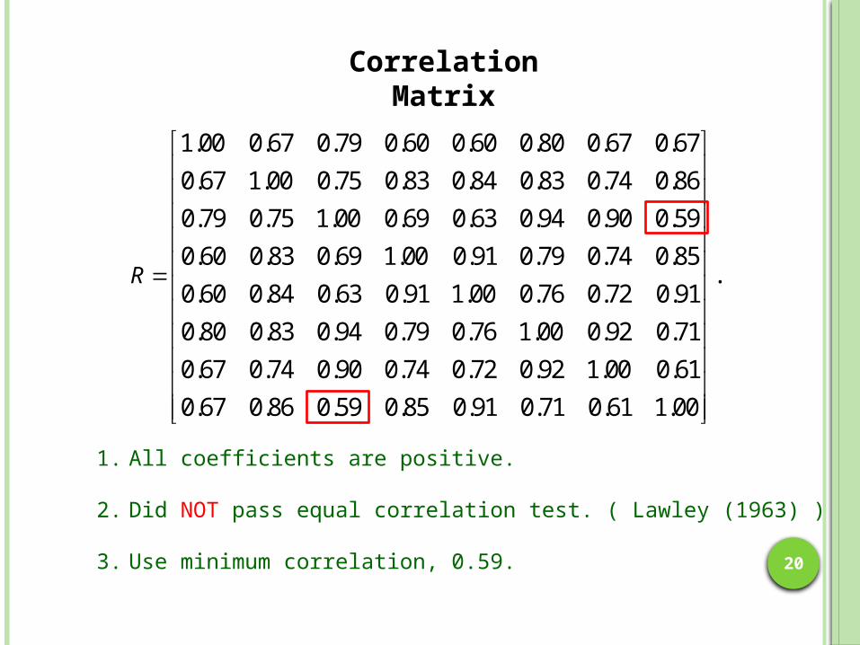
Correlation Matrix

1.00 0.67 0.79 0.60 0.60 0.80 0.67 0.67

0.67 1.00 0.75 0.83 0.84 0.83 0.74 0.86

0.79 0.75 1.00 0.69 0.63 0.94 0.90 0.59

0.60 0.83 0.69 1.00 0.91 0.79 0.74 0.85

0.60 0.84 0.63 0.91 1.00 0.76 0.72 0.91

0.80 0.83 0.94 0.79 0.76 1.00 0.92 0.71

0.67 0.74 0.90 0.74 0.72 0.92 1.00 0.61

0.67 0.86 0.59 0.85 0.91 0.71 0.61 1.00

5

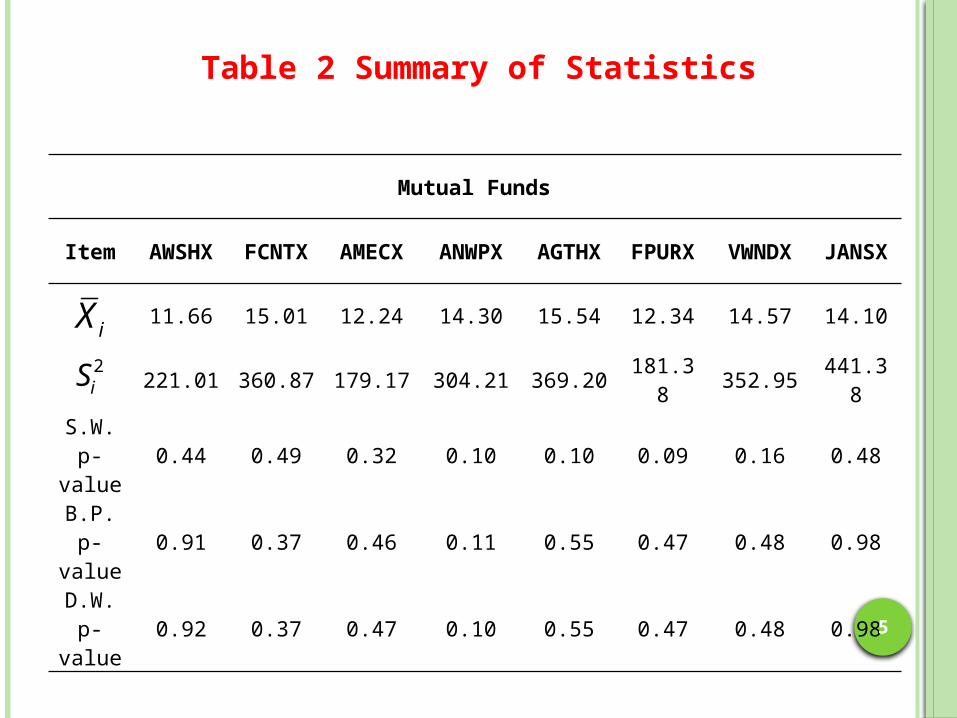
Mutual Funds

Item AWSHX FCNTX AMECX ANWPX AGTHX FPURX VWNDX JANSX

11.66 15.01 12.24 14.30 15.54 12.34 14.57 14.10

221.01 360.87 179.17 304.21 369.20 181.38 352.95 441.38

S.W.p-value 0.44 0.49 0.32 0.10 0.10 0.09 0.16 0.48

B.P.p-value 0.91 0.37 0.46 0.11 0.55 0.47 0.48 0.98

D.W.p-value 0.92 0.37 0.47 0.10 0.55 0.47 0.48 0.98

Table 2 Summary of Statistics

iX2iS

6

Contents

1. Literature Review

2. Optimal Confidence Region3. Application - Mutual Funds

4. Comparisons

5. Conclusions

7

Literature Review

1. Estimation of the Largest MeanSaxena, Krishna and Tong (1969)Dudewicz (1972)

2. Optimal Interval for the Largest MeanDudewicz and Tong (1971)Chen and Dudewicz (1976)Chen and Chen (2004)

3. Interval for the Largest Mean of Correlated Populations Chen, Li and Wen (2008)

4. Conf. Region for the Largest & Smallest MeansChen and Wu (2012)

8

k correlated populations (Treatments)

Means :

Common Vari. :2 ( > 0 )

Common Corr. : ( > 0 )

Random Vectors

, , , , 1, ,2X X X X l nl l kl

Distrib. of X2( , , )Nk

2( , , , )1 k

Confidence Region

9

Correlation Matrix

Sample Mean Vector

1 2, , ,

kX X X

Sample Covariance Matrix

1 ...

1

... 1

COR

11 12 1

21 22 2

1 2

...

...

k

kij

k k kk

COV

s s s

s s ss

s s s

10

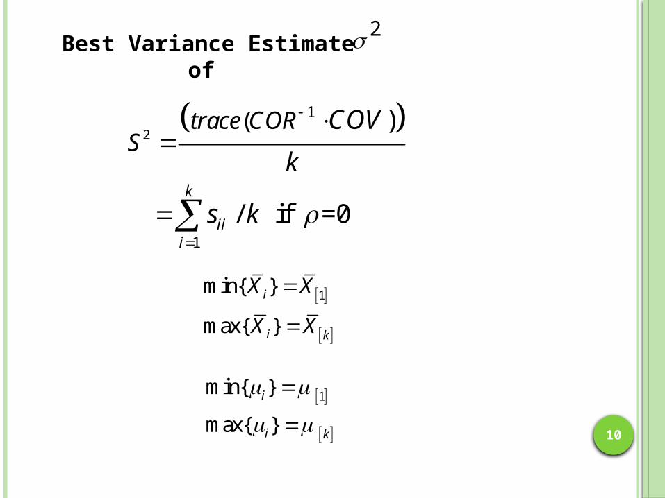
2

1

1

( )

/ if =0k

iii

trace CORS

COV

k

s k

Best Variance Estimate of 2

1min{ }

max{ }

i

i k

X X

X X

1min{ }

max{ }

i

i k

11

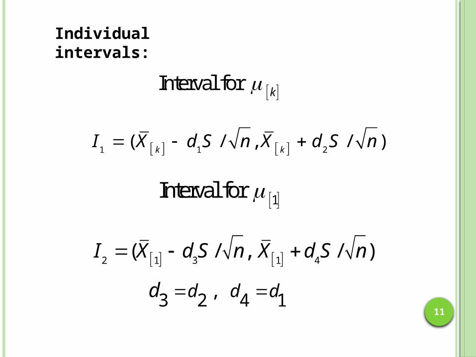
Individual intervals:

Interval for k

1 1 2( / , / )

k kI X d S n X d S n

2 1 3 1 4

,3 2 4 1

( / , / )

d d d

I X d S n X d S n

d

1Interval for

12

1 1 2 and ( )

kI I

1Confidence Region for and k

Goal:

13

Bonferroni Inequality

1

P all true 1 P at least one false

1 (1 ( true))

1- ( + ... )

1

i i

k

ii

A A

P A

k k k

1 2 1 2P 1

1- ( ) + 1- ( ) - 12 2

1

A and A P A P A

14

1 1 2( , )

kP I I

Using Bonferroni Inequality to obtain

1 22 ( / / ) 1

k k kP X d S n X d S n

2

*2 m i n ; , 1

over r

r d LF P

15

1 22 ( / / ) 1

k k kP X d S n X d S n

B y C h e n a n d C h e n (2004)

2

*2 min ; , 1

over r

r d LF P

16

2 10

2

; , { / 1

/ 1 ( ) ( )}

r

r

r d L d y

d y w g y dwdy

w

w

where

F

1 2

*

2

min1

; ,2over r

and L d d

PF r d L

17

18

Application

8 U.S. diversified mutual funds:

1. Washington Mutual (AWSHX)

2. Fidelity Contra (FCNTX)

3. American Income (AMECX)

4. New Perspective (ANWPX)

5. Growth Fund of American (AGTHX)

6. Fidelity Puritan (FPURX)

7. Vanguard Windsor (VWNDX)

8. Janus Family-Janus (JANSX)

19

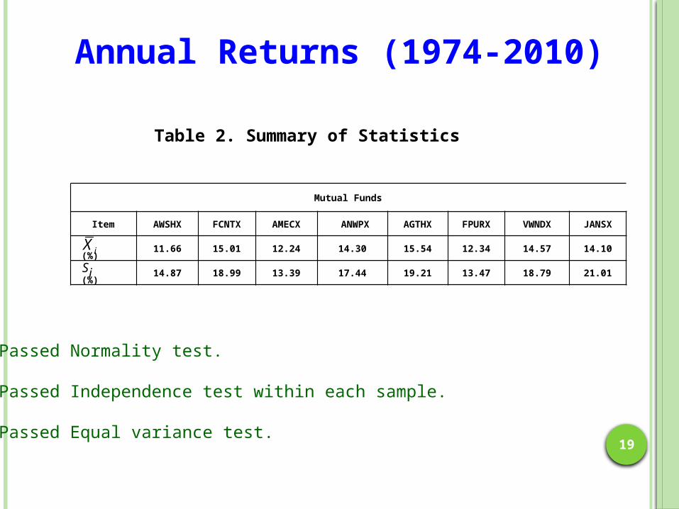
Annual Returns (1974-2010)

Table 2. Summary of Statistics

Mutual Funds

Item AWSHX FCNTX AMECX ANWPX AGTHX FPURX VWNDX JANSX

(%) 11.66 15.01 12.24 14.30 15.54 12.34 14.57 14.10

(%) 14.87 18.99 13.39 17.44 19.21 13.47 18.79 21.01

iX

Si

Passed Normality test.

Passed Independence test within each sample.

Passed Equal variance test.

20

Correlation Matrix

1.00 0.67 0.79 0.60 0.60 0.80 0.67 0.67

0.67 1.00 0.75 0.83 0.84 0.83 0.74 0.86

0.79 0.75 1.00 0.69 0.63 0.94 0.90 0.59

0.60 0.83 0.69 1.00 0.91 0.79 0.74 0.85

0.60 0.84 0.63 0.91 1.00 0.76 0.72 0.91

0.80 0.83 0.94 0.79 0.76 1.00 0.92 0.71

0.67 0.

R .

74 0.90 0.74 0.72 0.92 1.00 0.61

0.67 0.86 0.59 0.85 0.91 0.71 0.61 1.00

1. All coefficients are positive.

2. Did NOT pass equal correlation test. ( Lawley (1963) )

3. Use minimum correlation, 0.59.

21

2

1( )

=211.70

14.55

trace CORS

COV

k

S

8 max 15.54,AGTHX row. F. AmeriiX X G

1 22.36, 1.76d d

Critical values at P*=0.9 ( by Fortran ) :

1 min 11.66,AWSHX Washington MutualiX X

22

8 (15.54 2.36 14.55 / 37,15.54 1.75 14.55 / 37)

(9.89, 19.72) %

1 (11.66 1.75 14.55 / 37,11.66 2.36 14.55 / 37)

(7.48, 17.31) %.

and

90%Confidence Region for Best and Worst

23

Interpretation

1. The mutual fund AGTHX has the highest mean return.

2. The mutual fund AWSHX has the lowest mean return.

3. With a 90% confidence, the true highest mean return falls into the interval (9.89% to 19.72% ) and the lowest mean return falls into the interval (7.48% to 17.31%).

4. Both lower interval limits are much larger than the long-term bond rate of 3%.

5. Wide range of overlapping intervals, the mean returns among funds are not significantly different.

6. All of these funds are considered equivalent.

7. Investor’s choice : the ones with lower transaction and management fees.

24

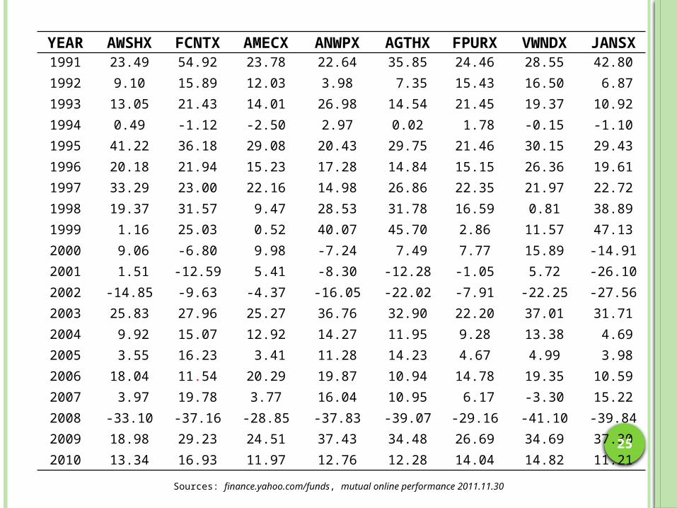
Appendix: Table 1 Annual Returns of 8 Mutual Funds in U.S. from 1974 to 2010

YEAR AWSHX FCNTX AMECX ANWPX AGTHX FPURX VWNDX JANSX1974 7.59 -14.05 -6.58 -19.43 -21.86 -12.16 -16.80 -6.981975 8.63 40.28 35.71 41.67 34.78 32.37 54.49 13.601976 5.87 36.51 35.19 16.16 18.70 30.82 46.41 20.001977 1.61 -10.91 -0.29 1.90 19.72 0.75 0.98 3.641978 -6.34 5.93 5.06 23.23 26.62 4.51 8.77 15.721979 -3.42 26.23 7.57 26.86 45.72 14.80 22.55 34.631980 24.02 29.88 9.87 25.51 39.64 20.29 22.62 51.571981 7.51 3.38 11.40 2.12 0.46 10.76 16.76 7.281982 34.69 17.18 36.24 21.54 25.69 29.09 21.72 30.631983 26.38 23.28 17.25 23.57 26.76 27.90 30.06 26.091984 8.42 -8.27 14.61 0.13 -5.51 8.81 19.47 -0.141985 32.17 27.06 27.79 34.29 27.05 28.71 28.03 24.551986 22.52 13.32 15.34 26.83 16.15 20.75 20.27 11.221987 1.42 -1.90 0.80 13.50 8.00 -1.79 1.23 4.201988 17.66 21.02 14.79 10.39 18.52 18.89 28.70 16.581989 28.96 43.15 22.94 26.09 30.01 19.60 15.02 46.321990 -3.81 3.94 -2.95 -2.08 -4.17 -6.35 -15.50 -0.74

25

YEAR AWSHX FCNTX AMECX ANWPX AGTHX FPURX VWNDX JANSX1991 23.49 54.92 23.78 22.64 35.85 24.46 28.55 42.80

1992 9.10 15.89 12.03 3.98 7.35 15.43 16.50 6.87

1993 13.05 21.43 14.01 26.98 14.54 21.45 19.37 10.92

1994 0.49 -1.12 -2.50 2.97 0.02 1.78 -0.15 -1.10

1995 41.22 36.18 29.08 20.43 29.75 21.46 30.15 29.43

1996 20.18 21.94 15.23 17.28 14.84 15.15 26.36 19.61

1997 33.29 23.00 22.16 14.98 26.86 22.35 21.97 22.72

1998 19.37 31.57 9.47 28.53 31.78 16.59 0.81 38.89

1999 1.16 25.03 0.52 40.07 45.70 2.86 11.57 47.13

2000 9.06 -6.80 9.98 -7.24 7.49 7.77 15.89 -14.91

2001 1.51 -12.59 5.41 -8.30 -12.28 -1.05 5.72 -26.10

2002 -14.85 -9.63 -4.37 -16.05 -22.02 -7.91 -22.25 -27.56

2003 25.83 27.96 25.27 36.76 32.90 22.20 37.01 31.71

2004 9.92 15.07 12.92 14.27 11.95 9.28 13.38 4.69

2005 3.55 16.23 3.41 11.28 14.23 4.67 4.99 3.98

2006 18.04 11.54 20.29 19.87 10.94 14.78 19.35 10.59

2007 3.97 19.78 3.77 16.04 10.95 6.17 -3.30 15.22

2008 -33.10 -37.16 -28.85 -37.83 -39.07 -29.16 -41.10 -39.84

2009 18.98 29.23 24.51 37.43 34.48 26.69 34.69 37.30

2010 13.34 16.93 11.97 12.76 12.28 14.04 14.82 11.21

Sources: finance.yahoo.com/funds, mutual online performance 2011.11.30

26

Interval for k

1 1 2( / , / )

k kI X c S n X c S n

2 1 3 1 4

,3 2 4 1

( / , / )

c c c c

I X c S n X c S n

1Interval for

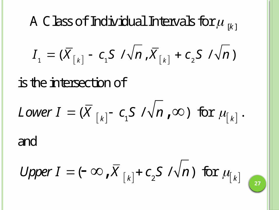
A Class of Individual Intervals

27

1

is the intersection of

( / ) for .

and

,k k

Lower I X c S n

2( / ) for ,

k kUpper I X c S n

1 1 2( / , / )

k kI X c S n X c S n

[ ]A Class of Individual Intervals for k

28

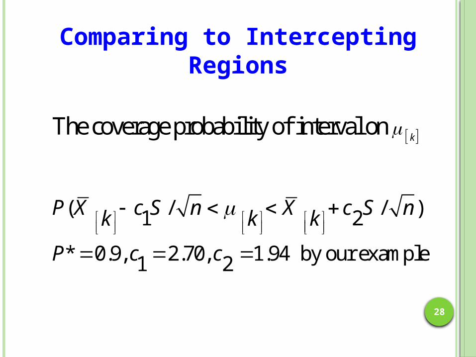
The coverage probability of interval on k

Comparing to Intercepting Regions

( / / )1 2

* 0.9, 2.70, 1.94 by our example1 2

P X c S n X c S nk k k

P c c

29

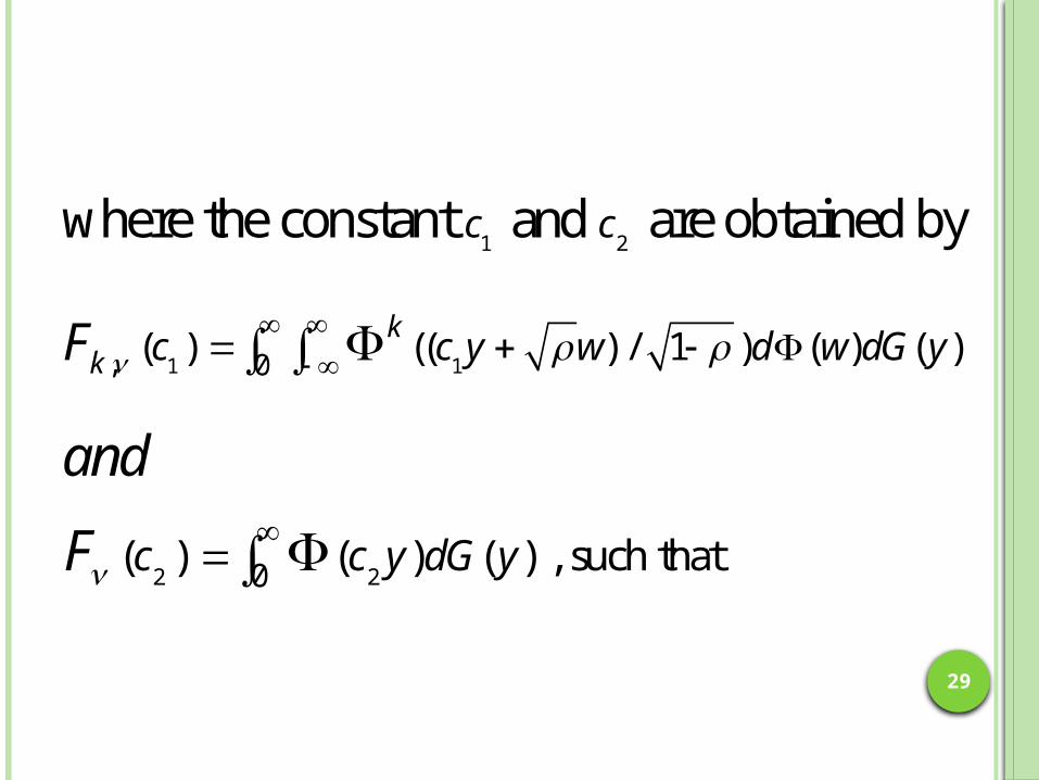
1 2where the constant and are obtained byc c

1 1, 0( ) (( ) / 1 ) ( ) ( )k

k c c y w d w dG yF

2 20( ) ( ) ( ) , such that

c c y dG y

and

F

30

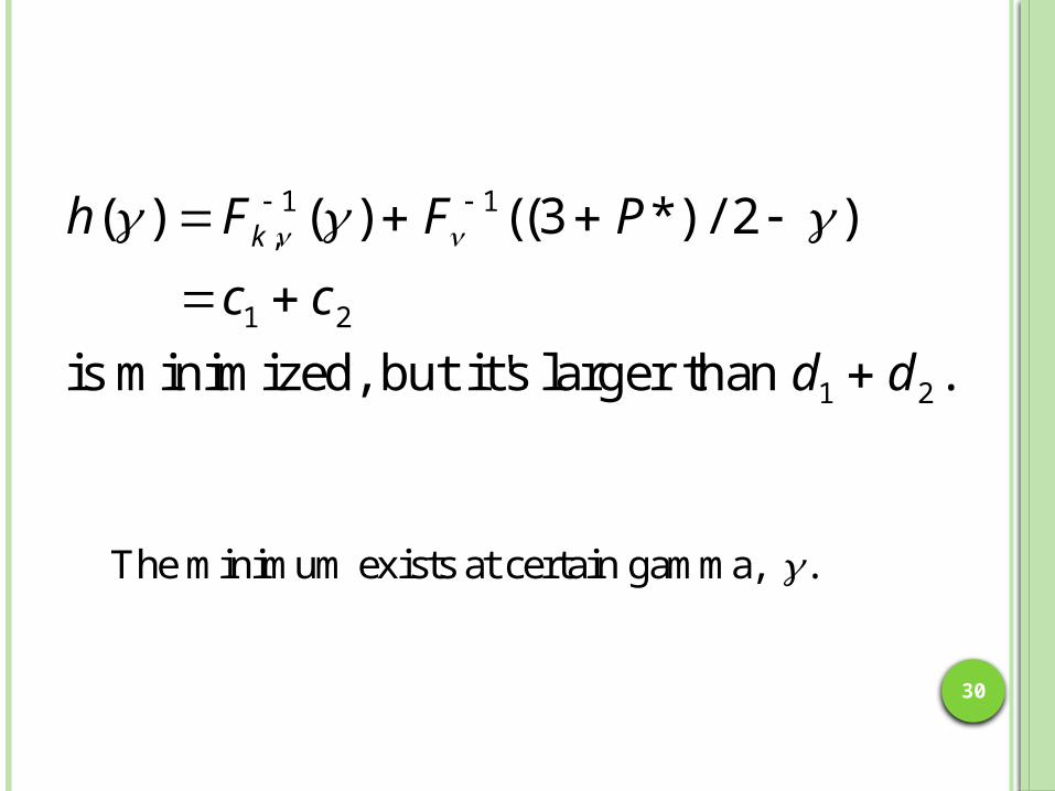
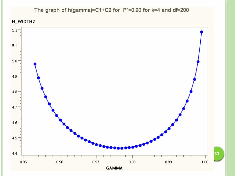
1 1,

1 2

1 2

( ) ( ) ((3 *) / 2 )

is minimized, but it's larger than .

kh F F P

c c

d d

The minimum exists at certain gamma, .

31

32

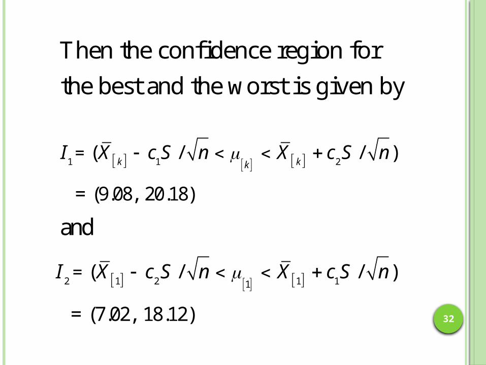
Then the confidence region for

the best and the worst is given by

1 1 2= ( / / )

= (9.08, 20.18)

and

k kkI X c S n X c S n

2 1 2 1 11= ( / / )

= (7.02, 18.12)

I X c S n X c S n

33

34

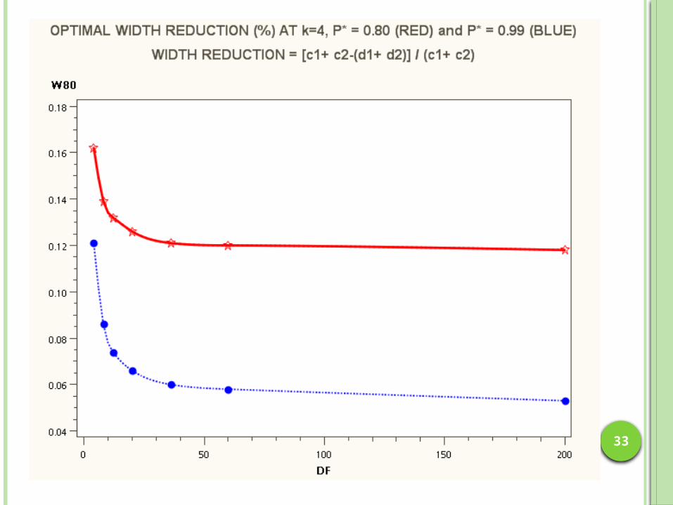
k υ P*=0.80 P*=0.90 P*=0.95 P*=0.99

3 3 0.16 0.14 0.13 0.133 9 0.12 0.10 0.09 0.073 30 0.11 0.09 0.08 0.063 210 0.11 0.08 0.07 0.054 4 0.16 0.14 0.13 0.124 12 0.13 0.11 0.09 0.074 36 0.12 0.10 0.08 0.064 200 0.12 0.09 0.08 0.058 8 0.16 0.14 0.13 0.108 24 0.14 0.12 0.10 0.078 40 0.14 0.11 0.09 0.078 240 0.14 0.11 0.09 0.0612 12 0.16 0.13 0.11 0.0912 36 0.14 0.11 0.10 0.0712 60 0.14 0.11 0.09 0.0712 240 0.14 0.11 0.09 0.06

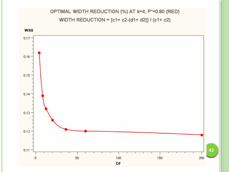
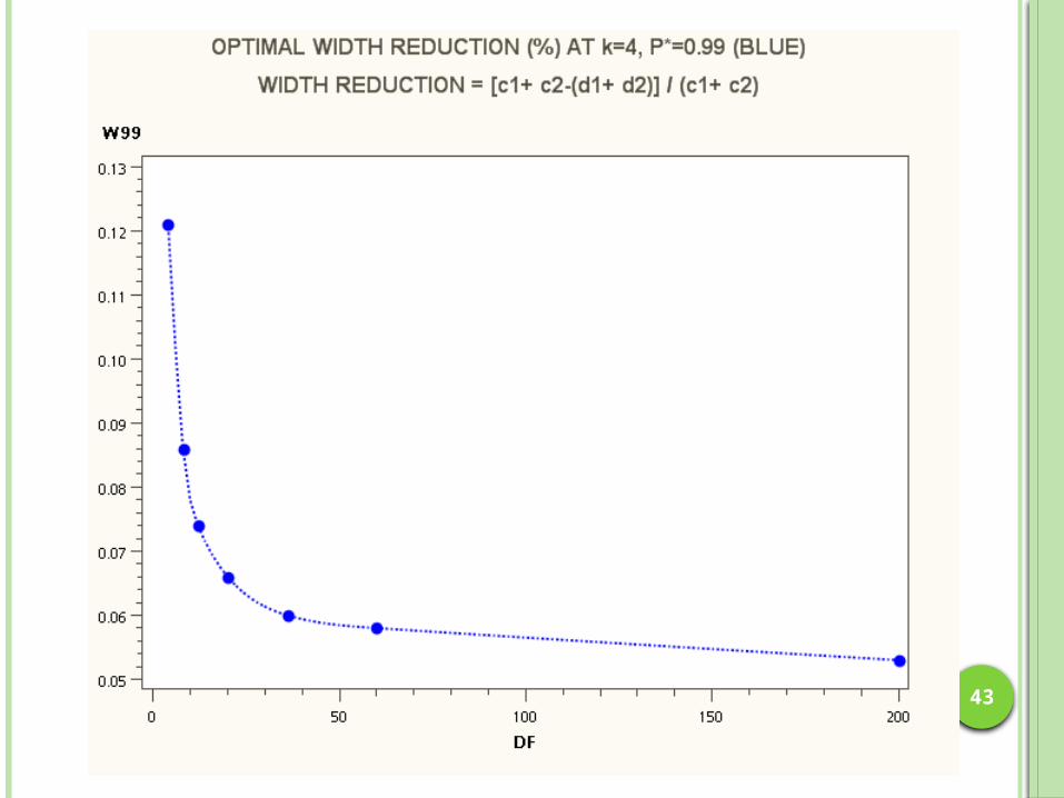
1 2 1 2 1 2Reduction = [( ) ( )] / ( )c c d d c c

35

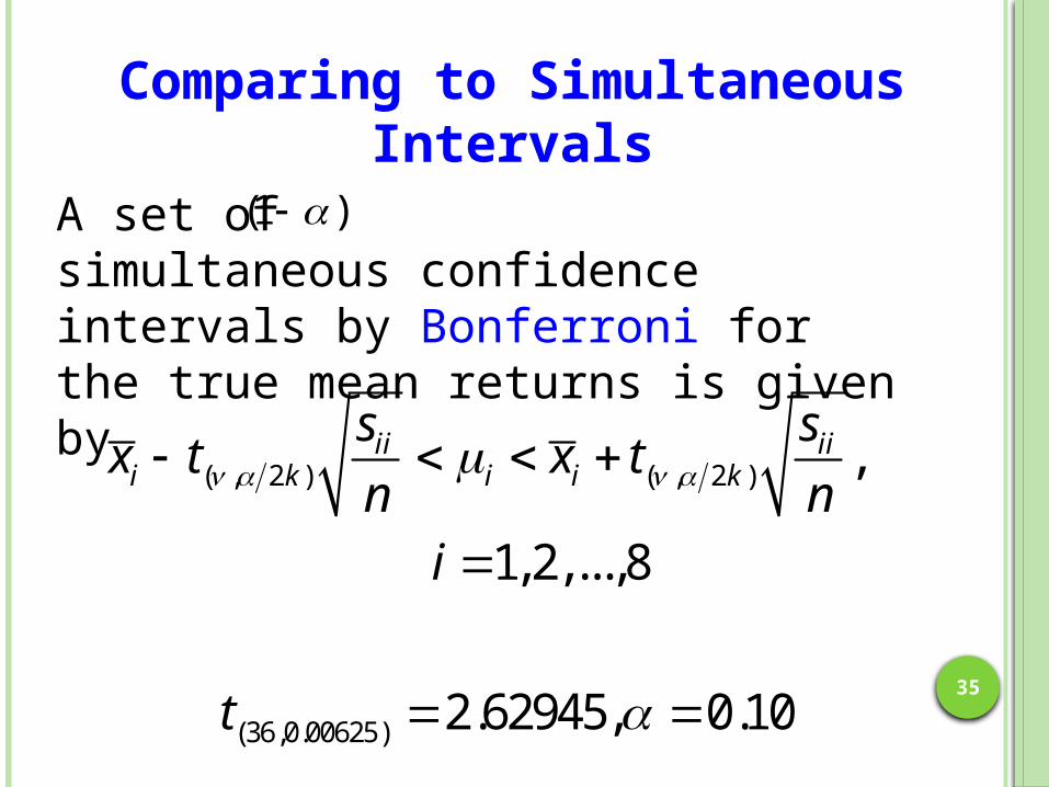
Comparing to Simultaneous Intervals

A set of simultaneous confidence intervals by Bonferroni for the true mean returns is given by

(1 )

( , 2 ) ( , 2 )

(36,0.00625)

,

1, 2,...,8

2.62945, 0.10

ii iii k i i k

s sx t x t

n ni

t

36

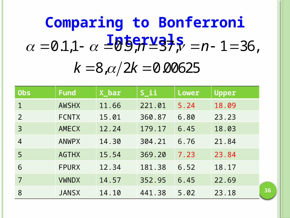
Comparing to Bonferroni Intervals

Obs Fund X_bar S_ii Lower Upper

1 AWSHX 11.66 221.01 5.24 18.09

2 FCNTX 15.01 360.87 6.80 23.23

3 AMECX 12.24 179.17 6.45 18.03

4 ANWPX 14.30 304.21 6.76 21.84

5 AGTHX 15.54 369.20 7.23 23.84

6 FPURX 12.34 181.38 6.52 18.17

7 VWNDX 14.57 352.95 6.45 22.69

8 JANSX 14.10 441.38 5.02 23.18

0.1,1 0.9, 37, 1 36,

8, 2 0.00625

n n

k k

37

Comparing to Bonferroni Intervals

Optimal intervals are shorter. AGTHX in (10.06, 18.86) Length=8.80AWSHX in ( 7.90, 16.70) Length=8.80

Bonferroni intervals are wider. AGTHX in (7.23, 23.84 ) Length=16.61AWSHX in (5.24, 18.09) Length=12.85

Intercepting intervals are medium shorter. AGTHX in (9.08, 20.18) Length=11.1AWSHX in (7.02, 18.12) Length=11.1

38

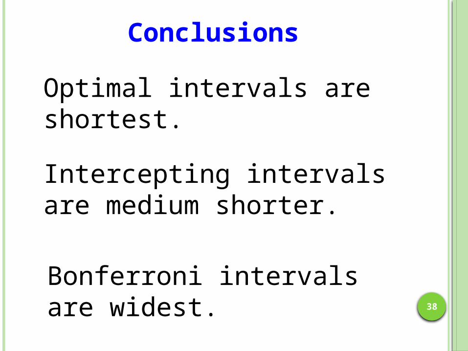
Conclusions

Optimal intervals are shortest.

Bonferroni intervals are widest.

Intercepting intervals are medium shorter.

39

References Bechhofer, R.E. (1954). A single-sample multiple decision procedure for ranking means of normal populations with

known variances. The Annals of Mathematical Statistics, 25, 16-39.

Chen, H.J. (1975). Strong consistency and asymptotic unbiasedness of a natural estimator for a ranked parameter Sankhya Ser. B, Vol. 38, 92-94.

Chen, H.J. and Chen, S.Y. (1999). A nearly optimal confidence interval for the largest normal mean. Communications in Statistics: Simulation and Computation, 28(1), 131-146.

Chen, H. J. and Chen, S. Y. (2004). Optimal confidence interval for the largest normal mean with unknown variance. Computational Statistics and Data Analysis, 47, 845-866.

Chen, H.J. and Dudewicz, E.J. (1976). Procedures for fixed-width interval estimation of the largest normal mean. Journal of the American Statistical Association, 71, 752-756.

Chen, H.J. and Dudewicz, E.J. (1973). Estimation of ordered parameters and subset selection. Technical Report, Ohio State University, Columbus, Ohio.

Chen, H.J., Li, H.L. and Wen, M.J. (2008). Optimal Confidence Interval for the Largest Mean of Correlated Normal Populations and Its Application to Stock Fund Evaluation. Computational Statistics and Data Analysis, 52, 4801-4813.

Chen, H.J., and Wu, S.F. (2012). A confidence region for the largest and the smallest means under heteroscedasticity. Computational Statistics and Data Analysis, 56, 1692-1702.

40

Dudewicz, E.J. (1972). Two-sided confidence intervals for ranked means. Journal of the American Statistical Association, 67, 462-464.

Dudewicz, E.J. and Tong, Y.L. (1971). Optimal confidence interval for the largest location parameter. Statistical Decision Theory and Related Topics. (S.S. Gupta and J. Yackel, Eds.) New York: Academic Press, Inc., 363-375.

Johnson, N.L. and Kotz, S. (1972). Distribution in Statistics: Continuous Multivariate Distributions. New York: Wiley.

Johnson, R.A. and Wichern, D.W. (2002). Applied Multivariate Statistical Analysis (4th Ed.), Upper Saddle River, New Jersey: Prentice Hall.

Lawley, D. N. (1963). On testing a set of correlation coefficients for equality. The Annals of Mathematical Statistics, 34, 149-151.

Saxena, K.M.L. (1976). A single-sample procedure for the estimation of the largest mean. Journal of the American Statistical Association, 71, 147-148.

Saxena, K.M.L., Krishna, M.L, Tong, Y.L. (1969). Interval estimation of the largest mean of k normal populations with known variance. Journal of the American Statistical Association, 64, 296-299.

Tong, Y.L. (1973). An asymptotically optimal sequential procedure for the estimation of the largest mean. The Annals of Statistics, 1, 175-179.

References

41

THANK YOU

FOR YOUR ATTENDANCE

42

43