an operational policy for a single vendor multi buyer

Louisiana State UniversityLSU Digital Commons

LSU Master's Theses Graduate School

2010

An operational policy for a single vendor multibuyer integrated inventory supply chain systemconsidering shipping timeChiranjit SahaLouisiana State University and Agricultural and Mechanical College, [email protected]

Follow this and additional works at: https://digitalcommons.lsu.edu/gradschool_theses

Part of the Construction Engineering and Management Commons

This Thesis is brought to you for free and open access by the Graduate School at LSU Digital Commons. It has been accepted for inclusion in LSUMaster's Theses by an authorized graduate school editor of LSU Digital Commons. For more information, please contact [email protected].

Recommended CitationSaha, Chiranjit, "An operational policy for a single vendor multi buyer integrated inventory supply chain system considering shippingtime" (2010). LSU Master's Theses. 3248.https://digitalcommons.lsu.edu/gradschool_theses/3248

https://digitalcommons.lsu.edu?utm_source=digitalcommons.lsu.edu%2Fgradschool_theses%2F3248&utm_medium=PDF&utm_campaign=PDFCoverPages

https://digitalcommons.lsu.edu/gradschool_theses?utm_source=digitalcommons.lsu.edu%2Fgradschool_theses%2F3248&utm_medium=PDF&utm_campaign=PDFCoverPages

https://digitalcommons.lsu.edu/gradschool?utm_source=digitalcommons.lsu.edu%2Fgradschool_theses%2F3248&utm_medium=PDF&utm_campaign=PDFCoverPages

https://digitalcommons.lsu.edu/gradschool_theses?utm_source=digitalcommons.lsu.edu%2Fgradschool_theses%2F3248&utm_medium=PDF&utm_campaign=PDFCoverPages

http://network.bepress.com/hgg/discipline/253?utm_source=digitalcommons.lsu.edu%2Fgradschool_theses%2F3248&utm_medium=PDF&utm_campaign=PDFCoverPages

https://digitalcommons.lsu.edu/gradschool_theses/3248?utm_source=digitalcommons.lsu.edu%2Fgradschool_theses%2F3248&utm_medium=PDF&utm_campaign=PDFCoverPages

mailto:[email protected]

AN OPERATIONAL POLICY FOR A SINGLE VENDOR MULTI BUYER INTEGRATED INVENTORY SUPPLY CHAIN SYSTEM

CONSIDERING SHIPPING TIME

A Thesis

Submitted to the Graduate Faculty of the Louisiana State University and

Agriculture and Mechanical College in partial fulfillment of the requirement for the degree of

Master of Science in Industrial Engineering

in

The Department of Construction Management and Industrial Engineering

By Chiranjit Saha

B.S., West Bengal University of Technology, Siliguri, India, 2006 August 2010

ii

ACKNOWLEDGEMENT

First of all, I wish to thank the Almighty for giving me the endurance to complete my

entire course. I want to express my deepest sense of gratitude to Dr. Bhaba R. Sarker, Elton G.

Yates Distinguished Professor of Industrial Engineering and Chairperson of my Committee, for

his invaluable guidance, constant encouragement, cooperative attitude, immense patience, useful

discussions during the course of research and preparation of the manuscript. He has always been

a fountain of inspiration to me.

Also, I am honored to express my esteem and profound sense of gratitude to Dr. Pius J.

Egbelu, Committee member and Professor of Industrial Engineering, for his constructive and

valuable suggestions. He was always quick to extend his help whenever I asked for it, and he

never failed to offer cooperative and accommodating services.

I am thoroughly delighted to recognize Dr. Lawrence Mann Jr., Professor Emeritus of

Industrial Engineering Department and Advisory Committee member, for his invaluable

suggestions endowed during the course of my research work.

I am also very proud to acknowledge Sukanta, Rakesh, Shantilal and Somesh, whose

constant help and collective efforts are undoubtedly reflected in the completion of this venture.

Also, nothing could have been possible without the incessant love, affection, sacrifice

and inspiration from my parents. I feel blessed to have such supportive parents, who were a

central force in guiding me to this day.

Finally, I would also like to devote my success to the financial assistance provided by the

CMIE Department in the form of assistantship during the tenure.

iii

TABLE OF CONTENTS

ACKNOWLEDGEMENT .............................................................................................................. ii

LIST OF TABLES .......................................................................................................................... v

LIST OF FIGURES ....................................................................................................................... vi

ABSTRACT .................................................................................................................................. vii

CHAPTER 1: INTRODUCTION ................................................................................................... 1 1.1 The Problem .......................................................................................................................... 2 1.2 Applications .......................................................................................................................... 3 1.3 Research Goals ...................................................................................................................... 4 1.4 Research Objectives .............................................................................................................. 5

CHAPTER 2: LITERATURE REVIEW ........................................................................................ 6 2.1 Single Vendor Single Buyer Supply Chain System .............................................................. 6 2.2 Single Vendor Multi Buyer Supply Chain System ............................................................... 8 2.3 Shortcomings of Previous Literature ................................................................................... 10

CHAPTER 3: MODEL DEVELOPMENT .................................................................................. 11 3.1 Assumptions ........................................................................................................................ 11 3.2 Notations ............................................................................................................................. 12 3.3 Model Formulation .............................................................................................................. 13 3.4 Model I: Item Shipped Right After Production ................................................................... 14

3.4.1 Average Inventory Calculation ..................................................................................... 15 3.4.2 Total Average Inventory Calculation ........................................................................... 17

3.5 Total Cost For Model I ........................................................................................................ 18 3.5.1 Ordering Cost ............................................................................................................... 18 3.5.2 Setup Cost ..................................................................................................................... 18 3.5.3 Inventory Carrying Cost ............................................................................................... 19 3.5.4 Transportation Cost ...................................................................................................... 20 3.5.5 Total System Cost ......................................................................................................... 21

3.6 Solution Methodology ........................................................................................................ 21 3.7 Sensitivity Analysis for Model I ......................................................................................... 23

3.7.1 Effect of S on ........................................................................................................ 24 ITC3.7.2 Effect of h on ........................................................................................................ 24 ITC3.7.3 Effect of P/D on ................................................................................................... 24 ITC

3.8 Model II: Items Are Shipped In Every Dg Period ........................................................... 25 3.8.1 Average Inventory Calculation ..................................................................................... 28 3.8.2 Total Average Inventory Calculation ........................................................................... 30

3.9 Total Cost for Model II ....................................................................................................... 31 3.9.1 Ordering Cost ............................................................................................................... 31 3.9.2 Setup Cost ..................................................................................................................... 31 3.9.3 Inventory Carrying Cost ............................................................................................... 32 3.9.4 Transportation Cost ...................................................................................................... 33

iv

3.9.5 Total System Cost ......................................................................................................... 34 3.10 Solution Methodology ...................................................................................................... 34

3.11 Sensitivity Analysis for Model II ...................................................................................... 35 3.11.1 Effect of S on ..................................................................................................... 36 IITC3.11.2 Effect of h on ..................................................................................................... 37 IITC3.11.3 Effect of P/D on ................................................................................................. 37 IITC

3.12 Model III: Items Shipped in Unequal Batches .................................................................. 38 3.12.1 Average Inventory Calculation ................................................................................... 40 3.12.2 Total Average Inventory Calculation ......................................................................... 43

3.13 Total Cost for Model III .................................................................................................... 43 3.13.1 Ordering Cost ............................................................................................................. 43 3.13.2 Setup Cost ................................................................................................................... 44 3.13.3 Inventory Carrying Cost ............................................................................................. 44 3.13.4 Transportation Cost .................................................................................................... 45 3.13.5 Total System Cost ....................................................................................................... 46

3.14 Solution Methodology ...................................................................................................... 47 3.15 Sensitivity Analysis for Model III ..................................................................................... 47

3.15.1 Effect of S on .................................................................................................... 48 IIITC3.15.2 Effect of h on .................................................................................................... 49 IIITC3.15.3 Effect of P/D on ................................................................................................ 50 IIITC

CHAPTER 4: RESULTS .............................................................................................................. 52 4.1 Performance Comparison .................................................................................................... 52 4.2 Comparison with Alternative Approach ............................................................................. 53

CHAPTER 5: RESEARCH SUMMARY AND CONCLUSIONS .............................................. 54 5.1 Conclusions ......................................................................................................................... 54 5.2 Research Significance ......................................................................................................... 55 5.3 Possible Future Extensions.................................................................................................. 55

BIBLIOGRAPHY ......................................................................................................................... 57

APPENDIX ................................................................................................................................... 60

VITA ............................................................................................................................................. 63

v

LIST OF TABLES

Table 1: Data for single vendor 9 buyers problem ........................................................... 22

Table 2: Summary of results ............................................................................................. 22

Table 3: Effect of P/D (= A) ratio on ........................................................................ 26 ITC



Table 6: Effect of P/D (= A) ratio on ....................................................................... 39 IITC



Table 9: Effect of P/D (= A) ratio on ...................................................................... 51 IIITC

Table 10: Data for single vendor 9 buyers problem ......................................................... 52

Table 11: Summary of results ........................................................................................... 52

Table 12: Performance comparison with alternative models ............................................ 53

vi

LIST OF FIGURES

Figure 1.1: Flow diagram of a single vendor multi buyer integrated supply chain ............ 2

Figure 3.1 Inventory flow in Model I ............................................................................... 15

Figure 3.2: Graphical representation of .................................................................... 23 ITC

Figure 3.3: Effect of P/D (= A) ratio on ................................................................... 26 ITC

Figure 3.4 Inventory flow in Model II .............................................................................. 27

Figure 3.5: Graphical representation of .................................................................. 36 IITC

Figure 3. 6: Effect of P/D (= A) ratio on .................................................................. 39 IITC

Figure 3.7 Inventory flow in Model III ............................................................................. 41

Figure 3.8: Graphical representation of .................................................................. 49 IIITC

Figure 3.9: Effect of P/D (= A) ratio on .................................................................. 51 IIITC

vii

ABSTRACT

Since its introduction, the concept of integrated inventory supply chain has received a

considerable amount of attention. The majority of studies in the last three decades revealed an

increase in holding cost as product moves further down the chain or up the chain. A recent study

Hoque (2008) considered vendor’s setup cost and inventory holding cost. Some research also

considered fixed transportation cost, which is unrealistic. This study focuses on a single-vendor,

multi-buyer scenario and presents three models. First, two models illustrate the transferring of

equally-sized batches. Then, a third model considers the transferring of unequally-sized batches

in a lot. This study relaxes the assumption that vendor’s holding cost must be greater than or less

than all buyer’s holding costs in the system. Also, this research facilitates unequal transportation

time and cost for different buyers for greater flexibility. The total system cost is calculated by

summing the annual operational cost for all the parties in the system. Optimum values of the

decision variables are determined using a direct search method. As presented by the third model,

a numerical example demonstrates that the total system cost is less when compared with other

two models presented. This study also presents the following: solution procedures to solve each

model, many numerical examples to support mathematical findings, and performance

comparisons among three findings. In order to justify the lot-splitting approach for solving the

integrated inventory problem, alternative models with no lot splitting are devised and tested

under the same circumstances. Alternative models with no lot splitting produce similar or better

results. Under the same circumstances, the alternate third model is observed to be offering the

least total cost for the system. This study also presents a sensitivity analysis to check the

robustness of the three models. The future extension of this research may involve considering

storage capacity constraint and random demand.

1

CHAPTER 1

INTRODUCTION

Consider a single vendor supplying an item to multiple buyers. The vendor produces

the item in batches and at a finite rate. The vendor then sends the finished items to multiple

buyers. In this process, the vendor incurs batch set-up and transportation cost, and the

vendor and buyer both carry the item holding cost proportional to time. Meanwhile, each

buyer has his own deterministic yearly demand. In this scenario, the buyer has a problem

with determining the ordering quantity, and the vendor has a problem with determining

optimum production quantity and shipping schedule, which minimizes the operating cost.

During the last three decades, researchers have been searching for the solution to these

problems. Researchers have shown that by viewing the vendor and buyers as a system (also

known as integrated supply chain) rather than as separate individuals, total system cost can

be reduced significantly. The basis of the integrated supply chain concept is that each buyer

has clear knowledge about their yearly demand, and buyers are ready to share this

information with the supplier to enjoy the benefits of coordination. Today, great

improvements in electronic information exchange have made this concept feasible.

In supply chain, transportation cost is a major part of operational cost.

Transportation time, cost, and capacity constraint play a role in making decisions. In today’s

world, short life cycle and countless specialties of similar products have made the global

market highly competitive. In order to survive market pressure, every company has to be

highly competitive in terms of product quality, price and product supply. The flow diagram

of a single vendor multi buyer supply chain system is shown in Figure 1.1.

2

Buy

er 1

B

uyer

2

Buy

er 3

B

uyer

m

Transport Vehicle Vendor

Figure 1.1: Flow diagram of a single vendor multi buyer integrated supply chain

1.1 The Problem For decades, the primary objectives among research have been determining the

optimal batch size, numbers of batch sizes in a lot, number of lots per year, and shipping

schedule of integrated inventory models. The majority of this research is done with ideal

assumptions. In both single and multistage supply chains, decision parameters,

transportation time, cost and yearly demand vary with time. Demand of an individual buyer

can be different, and holding cost and shipping cost may also vary. An individual buyer’s

economic order quantity and shipping schedule are also likely to differ. Unwise choices of

these variables can lead to excessive product costs, which, in turn, can lead to customer

dissatisfaction and lost sales.

The present research focuses on determining economic ordering quantity (EOQ) and

shipping strategy of an inventory system integrated with a single-product, single-vendor,

3

and multi-buyer. In a single-vendor-multi-buyer system, a vendor produces and delivers an

item to multiple buyers. Depending on the demand of all buyers, production and shipping

policies are determined. If, for the sake of simplicity, we set a universal ordering quantity

for all buyers, then we may fail to optimize everyone’s cost. Some buyers may receive

more than they need in a particular time span while others may receive less than needed.

Again, imagine buyers are spread across the country where shipping cost and time varies

significantly among buyers. For example, buyers who are far from the vendor need to ship

earlier than those buyers who are relatively close to vendors. But maintaining different

schedules for all buyers is difficult to accommodate, so we must find a cost-effective policy

that better controls the complexity of operation. Also, we must determine how to regulate

batch size in such a way that not only reduces ordering cost, setup cost and holding cost, but

also avoids shortage.

1.2 Applications

Automobiles are an example of such an item. All the showrooms around the country

receive shipment of cars from the vendor. Suppose a manufacturing facility is in Michigan,

and some of the showrooms are in Indiana, Louisiana or Alaska. Shipping cost and time is

different for each case, and each showroom requires space for display, which requires high

maintenance and surveillance cost. It is obvious that cost in California is more than that in

Oklahoma or Missouri. No dealer likes to keep an excess of inventory because such

inventory increases the holding cost. Again, if we look around we note, multiple showrooms

with same automobiles which results in competition. No dealer can afford to not having cars

in demand because the customer has a choice to get another next door. It is important that

the dealer gets the shipment on time.

4

Another problem is every showroom has its own demand; based on ordering cost

and holding cost, the showrooms’ economic order quantities differ from one another. Again,

considering setup cost and holding cost, vendor’s economic manufacturing quantity in a

batch can be different from the EOQ of all the showrooms. Now, if we arbitrarily assign

each showroom the same shipping quantity and schedule, the system is likely to fail. The

vendor interest is to produce as many items and ship them to the retailer as soon as possible

to avoid holding cost. The interest of the retailer is to get the right amount of product within

the right timeframe to avoid holding cost and other miscellaneous expenses. Again,

transferring items in smaller lots results in lower inventory cost but higher ordering, setup,

and transportation cost. On the other hand, transferring items in larger lots leads to higher

inventory cost but lower ordering, setup, transportation cost, and scheduling interferences

due to scarce storage capacity for both the vendor and the buyer.

Some examples of such industries are BMW, Ford, GMC, Mercedes, and Toyota,

which produce cars, trucks, and other motorized vehicles. The proposed research will

improve the inventory management of the supply chain system, which will also significantly

reduce the system’s operating cost and increase its profitability.

1.3 Research Goals

The objective of this research is to study and model a single-vendor-multi-buyer

inventory system, which constrains the transport capacity and maintains various

transportation times between different buyers. In realistic situations, inventory holding

costs are different for vendors and buyers; these transportation costs affect ordering policy,

production policy, and total system cost, and transportation costs vary among all buyers.

This research presents an operational policy to produce and deliver items in the right

quantity at the right time while reducing the total system cost.

5

1.4 Research Objectives

This problem addresses production and shipping policies of a product that flows

from a vendor to multiple buyers. Yearly demands for all the buyers are recorded and are

deterministic. Vendor and buyers maintain a close relationship to reduce overall system

cost. In this research, three models are presented to address the problem under different

operational policies. The vendor sends the product to buyers in multiple batches. Batches

could be equally or unequally sized. Carrying costs for the vendor and each buyer may vary

depending on their geographic location. Transportation time and cost for each buyer differs.

Due to the above reasons, the nature of inventory of this supply chain system differs from

traditional systems. Hence, the primary objectives of this research are:

(i) To study the behavior of the inventories under three operational policies.

(ii) To find optimal batch size.

(iii) To find optimal batch number in a lot.

(iv) To find best policy to reduce total system cost among three operational policies.

6

CHAPTER 2

LITERATURE REVIEW

This study has only considered the deterministic demand. The literature review

organizes previous research in chronological order starting with the simplest, single-product,

single-vendor, single-buyer scenario, unrestricted production rate and lot-for-lot policy

(Goyal 1976). The review then shifts to the most recent single-vendor, multi-buyers

scenario, which also involves setup and inventory cost for the vendor with finite production

rate (Hoque 2008). Among the previous works, differences are mainly assumptions of

production rate and replenishment period. Recently, other aspects of this problem have also

been discussed in the literature. Other aspects refer to multiple buyers, transportation

capacity and cost, lead time, variable production cost, quality and process failure, set up cost

reduction and more realistic demand rates.

2.1 Single Vendor Single Buyer Supply Chain System

Goyal (1976) proposed his first model, addressing an integrated supply chain,

assuming an infinite production rate, a uniform deterministic demand over time. He ignored

lead time and restricted stock outs. In his research, the vendor produces in lots and sends the

entire lot to the retailer. This process implies that the entire lot must be produced before

shipment. Banerjee (1986) kept that lot-for-lot policy, but relaxed the assumption of infinite

production rate. Banerjee (1986) also “coined” the term, “JELS” (joint Economic Lot

Sizing) and argued about economic benefits of both vendor and retailer through JELS.

Banerjee (1986) considered purchase transmit time, setup time and delivery time in

accordance with actual production time. Goyal (1988) introduced a more generalized JELS

model, which relaxed the assumption of lot-for-lot model and proposed to produce in a lot

which can be supplied in “n” integer number of orders after the entire lot is produced. Goyal

7

(1988) showed that his joint total relevant cost is less than or equal to that of the JELS

model. Goyal (1995) used a different approach than equally-sized shipment to come up with

an idea of geometric shipment size. This means that the successive shipment size is the

product of the prior shipment size in relation to the ratio of production and demand rate.

Viswanathan (1998) presented two models: one in which the shipment sizes are similar and

another in which the shipment size is equal to whatever inventory is available at that point.

In this study Viswanathan named Lu’s (1995) equal shipment size policy as “Identical

delivery quantity” (IDE) and Goyal’s (1995) an unequal shipment size model as “deliver

what is produced” (DWP). Viswanathan showed that neither policy is better than the other

for all type of problems, and he concluded that the best policy depends on the problem’s

parameters.

Goyal and Nebebe (2000) pointed out the difficulties faced by the vendor and

retailer while applying the policy proposed by Goyal (1995) and Hill (1997), who pointed

out the difficulty of determining batch size for the vendor, optimal number of shipments,

and each shipment size for the buyer. Goyal and Nebebe (2000) proposed an alternate

solution which suggests that among “n” shipments, the first shipment is smaller and

followed by (n-1) equal- sized, which is equal to the product of the first shipment size as

well as its rate of production over rate of demand. Goyal (2000) extended the policy

proposed by Hill (1997). He proposed that the following shipment sizes will be determined

by first shipment size. The following shipment sizes may be increased by a factor of

production rate over demand rate until it is impossible to do so. A likely drawback of this

study is that the intended application of the model is unclear. Hill and Omar (2006)

presented derivation of optimal manufacturing batch size and shipment policy when

product-holding cost increases as the product moves down to the buyer under non-required

8

equal shipping size. Zhou and Young (2007) relaxed the assumptions that vendor’s stock

holding is always greater than the retailer’s. They showed that their model performs equally

well in reducing average total cost regardless of the vendor’s or retailer’s stockholding

costs, which are never equal to each other. In this study they also allowed shortages but

only for buyers. They also presented a production inventory policy for deteriorating items.

In this study they proved that the optimal policy for vendors whose holding costs are greater

than the retailers’ holding cost is that all unequally-sized shipments increase the following

shipments by ratio of production rate to the demand rate. Pan and Young (2002) explored

how to reduce lead-time in an integrated system involving cost. They argued that better

customer satisfaction levels and reduced safety stock levels can be achieved through

improving lead-time; however, these changes occur at the expense of lead-time crashing

cost. This study developed a model, which yields lower total cost and reduced lead time

than that presented by Banerjee (1986) and Goyal (1988). Ultimately, this research is an

extension of Goyal (1988), and it relaxed the infinite production capacity assumption.

Hoque and Goyal (2000) considered transport capacity limitation by presenting an optimal

policy for the single-vendor and single-buyer integrated supply chain, which considers equal

and unequal shipment size and transportation capacity.

2.2 Single Vendor Multi Buyer Supply Chain System

Joglekar and Tharthare (1990) considered another area of integrated supply chain,

i.e., single vendor and multi buyer. In that study they presented an alternate solution of the

same problem considered by Banerjee (1986) and named it as the ‘Individual Responsible

and Rational Decision’ (IRRD). In IRRD, they refined JELS by breaking set-up cost into

vendors’ order processing and handling cost per production run setup cost. Based on the

changes, the authors claimed IRRD’s consistency in a free enterprise scenario and

9

superiority over Banerjee’s (1986) JELS model in dealing with problems like single-vendor

and non-identical buyers. A single-vendor, multi-retailer problem is also addressed by

Affisco et al. (1988, 1991, and 1993). In these studies, researchers addressed the single

vendor and many identical retailers with an objective of reducing production setup cost and

retailer’s ordering cost. They showed that substantial improvement can be achieved, under

this model, through the independent cost optimization technique; thus, in a cooperative

environment, an integrated inventory approach is suggested over independent cost

optimization. Lu (1995) proposed his model in context of a single-vendor or multi-buyers

scenario. Lu allowed shipments during production and ignored Goyal’s assumption of

producing an entire lot before shipment. Many other JELS-based models, e.g. Baneerjee and

Kim (1995) and Kim and Ha (2003), considered equally-sized shipment policy. Yau and

Chiao (2004) presented a model in which the vendor produces and supplies to all the buyers;

this minimizes the vendor’s total annual cost based on the maximum cost buyers are willing

to incur. They came up with an efficient algorithm to search an optimal cost curve. Siajadi et

al. (2005) presented a single-vendor-multi-buyer scenario in which the vendor is the sole

supplier for a specific item to all buyers. Supplies are delivered in equal sizes, but the

shipment size may differ from one buyer to another based on their demand. Supplies are

delivered in sequence; e.g., the first buyer will get first supply followed by second and third

and so on, assuming production-cycle time and buyer’s-ordering cycle time are the same.

Also, the time between one delivery and the next is fixed for each buyer. Hoque (2008)

presented single-vendor multi-buyer system considering and considered vendor’s setup and

inventory holding cost. In this research, he argued in favor of transferring of smaller lots

over larger lots when storage capacity is scarce for both the vendor and the buyer.

Viswanathan and Piplani (2001) addressed the same problem and tried to solve it by using a

10

game theoretic approach. They proposed that vendors will specify the common

replenishment period for accepting the proposal, and in turn, buyers will receive a price

discount from the vendor. The price discount will be sufficient to compensate the alleviated

product carrying cost, if any. Viswanathan and Piplani (2001) derived optimal

replenishment period and price discount quantity by solving Stackelberg game.

Chen et al. (2009) discussed delivery and shared transportation cost in a multiple-

vendors integrated inventory system, and Comeaux et al. (2005) discussed the product

quality inspection policy in an integrated inventory system.

2.3 Shortcomings of Previous Literature

This literature review briefly recalls the development of the integrated supply chain

management systems starting from the simplistic single-vendor, single-buyer system and

moving toward more advanced single-vendor, multiple-buyers systems. The review points

out that each study has its own shortcomings. Realistically, most of the problems are

constrained. A vendor’s holding cost could be higher or lower than other buyers’ in the

same system; transportation time to one buyer could be different from another buyer, and

even transportation cost may differ among buyers. Although many researchers considered

constraints mentioned above in their models one at a time, so far, they have given little

attention to building a single-vendor-multiple-buyer integrated model, which considers all

the above mentioned constraints. Here, we present a single-vendor-multi-buyer integrated

supply chain model with equal and unequal batch sizes; this model considers vendor’s set-

up cost, transportation time, cost, capacity constrained and unequal holding cost for buyers.

Three models are presented: the first two, which consider equal batch size and the third

model, which considers unequal batch size.

11

CHAPTER 3

MODEL DEVELOPMENT

In this section the formulation of the three operational models are presented to

illustrate different production and shipping policies. These models are based on some

previously described assumptions and notations and are followed by average inventory and

total system cost derivations.

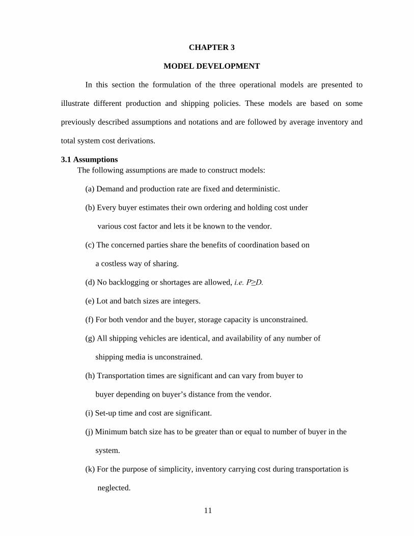
3.1 Assumptions The following assumptions are made to construct models:

(a) Demand and production rate are fixed and deterministic.

(b) Every buyer estimates their own ordering and holding cost under

various cost factor and lets it be known to the vendor.

(c) The concerned parties share the benefits of coordination based on

a costless way of sharing.

(d) No backlogging or shortages are allowed, i.e. P≥D.

(e) Lot and batch sizes are integers.

(f) For both vendor and the buyer, storage capacity is unconstrained.

(g) All shipping vehicles are identical, and availability of any number of

shipping media is unconstrained.

(h) Transportation times are significant and can vary from buyer to

buyer depending on buyer’s distance from the vendor.

(i) Set-up time and cost are significant.

(j) Minimum batch size has to be greater than or equal to number of buyer in the

system.

(k) For the purpose of simplicity, inventory carrying cost during transportation is

neglected.

12

3.2 Notations

The following notations will be required to formulate the model:

ith buyer parameter

ia Ordering cost ($/order)

itC Cost of one vehicle for buyer ($/vehicle) thi

iD Annual demand (unit/year)

id Daily demand of ith buyer (unit/day)

ih Holding cost per item per year ($/unit/year)

tq Vehicle capacity (units/vehicle)

it Shipping time to ith buyer (days)

Vendor Parameter

D Annual rate of demand (unit/year)

g Smallest batch size

h Holding cost per item per year ($/unit/year)

P Production rate per year ( kDPDP => /, ), (unit/year)

S Setup cost ($/setup)

Variables

ig Original shipping size for ith buyer

iG Shipping size for ith buyer which includes transportation time demand

g Smallest batch size

G Batch size which includes transportation time demand for m buyers

n Number of equal or unequal batches in a lot

13

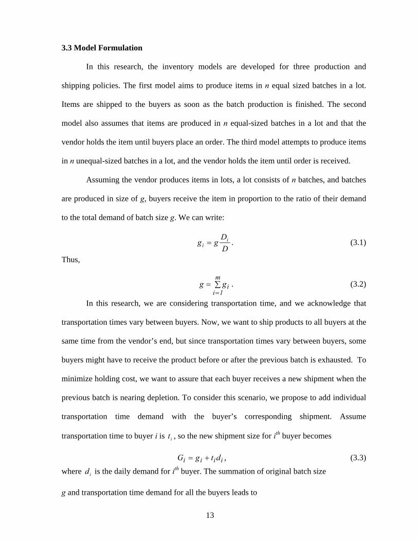
3.3 Model Formulation

In this research, the inventory models are developed for three production and

shipping policies. The first model aims to produce items in n equal sized batches in a lot.

Items are shipped to the buyers as soon as the batch production is finished. The second

model also assumes that items are produced in n equal-sized batches in a lot and that the

vendor holds the item until buyers place an order. The third model attempts to produce items

in n unequal-sized batches in a lot, and the vendor holds the item until order is received.

Assuming the vendor produces items in lots, a lot consists of n batches, and batches

are produced in size of g, buyers receive the item in proportion to the ratio of their demand

to the total demand of batch size g. We can write:

DD

gg ii = . (3.1)

Thus,

∑==

m

1iigg . (3.2)

In this research, we are considering transportation time, and we acknowledge that

transportation times vary between buyers. Now, we want to ship products to all buyers at the

same time from the vendor’s end, but since transportation times vary between buyers, some

buyers might have to receive the product before or after the previous batch is exhausted. To

minimize holding cost, we want to assure that each buyer receives a new shipment when the

previous batch is nearing depletion. To consider this scenario, we propose to add individual

transportation time demand with the buyer’s corresponding shipment. Assume

transportation time to buyer i is , so the new shipment size for ith buyer becomes it

iiii dtgG += , (3.3) where is the daily demand for ith buyer. The summation of original batch size id

g and transportation time demand for all the buyers leads to

14

. (3.4) ∑=

+=m

iii dtgG

1

3.4 Model I: Item Shipped Right After Production

As described above, a vendor ships items to buyers as soon as the batch is produced.

In the first model, we are assuming all batch sizes in a lot are equal and that there are n

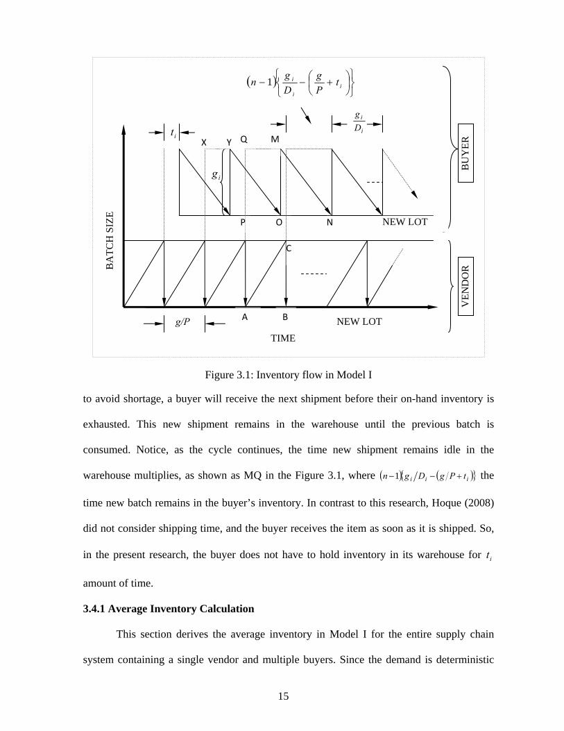
batches in a lot. Figure 3.1 shows the production and inventory flow for the first model.

In Figure 3.1, Pg , ii Dg , and are the time segments, which represent the

following: production time for a batch, consumption time for buyer and transportation

time for buyer, respectively. In Figure 3.1, triangle (ABC) represents the inventory for

the vendor. The triangle (MNO) represents the ideal inventory for the thi buyer when an item

is received at the end of previous inventory. The area (MOPQ) with a dashed line represents

inventory in the buyers’ warehouse while the previous batch is being consumed.

it

thi

thi

In the beginning of the cycle, the vendor begins production at a finite rate, and

inventory begins to accumulate at a constant rate. In Figure 3.1, the slope AC is the rate of

build inventory during production. As soon as production of the batch is complete, items are

shipped to each buyer, and inventory of vendor reduces to zero. At this point, the vendor

produces the next batch, repeating the process until the entire lot is produced. Although

items to all buyers are shipped at the same time, they will receive them after time, since

shipping time differs among the buyers. Items are available for consumption as soon as the

buyer receives them; and, the buyer consumes the item at a constant rate. In Figure 3.1,

slope MN is the consumption rate. Since a buyer consumes items at a fixed rate, on-hand

inventory starts decreasing at a constant rate. Again, as we assumed and

it

gDP > DgP // <

15

it

A B

C

M

N O P

Q

ig

X Y

( )⎭⎬⎫

⎩⎨⎧

⎟⎠⎞

⎜⎝⎛ +−− i

i

i tPg

Dgn 1

g/P

BU

YER

V

END

OR

i

i

Dg

TIME

BA

TCH

SIZ

E

NEW LOT

NEW LOT

Figure 3.1: Inventory flow in Model I

to avoid shortage, a buyer will receive the next shipment before their on-hand inventory is

exhausted. This new shipment remains in the warehouse until the previous batch is

consumed. Notice, as the cycle continues, the time new shipment remains idle in the

warehouse multiplies, as shown as MQ in the Figure 3.1, where ( ) ( ){ }iii tPgDgn +−−1 the

time new batch remains in the buyer’s inventory. In contrast to this research, Hoque (2008)

did not consider shipping time, and the buyer receives the item as soon as it is shipped. So,

in the present research, the buyer does not have to hold inventory in its warehouse for

amount of time.

it

3.4.1 Average Inventory Calculation

This section derives the average inventory in Model I for the entire supply chain

system containing a single vendor and multiple buyers. Since the demand is deterministic

16

and prohibits backlog or shortage, the production rate must be greater than the demand rate.

The total system inventory consists of buyer’s inventory, and vendor’s inventory, . bI mI

(a) Buyer’s Average Inventory Calculation

Each buyer receives amount of an item in each shipment and takes ig

ii Dg amount of time to consume it. So, each buyer’s average inventory for the first batch

is ( ii Dg 22 ). Since the second shipment arrives before the first shipment is finished, the

buyer must hold the second shipment for { })( iii tPgDg +− additional amount of time

until previous shipment is consumed. Therefore, average inventory during the second

shipment is [ { (− } iiiiii gtPgDgDg )22 ++ ]. The third shipment arrives before the

second shipment is finished and actually remains in the warehouse twice the time of the

second shipment. In Figure 3.1, we can see QM is double of XY, which are the current

times in which shipping remains idle in the warehouse. This continues until the entire lot is

supplied, if there are batches in a lot, then the nth shipment must remain in the warehouse

for

n

{ )()1( iii tPgDgn +−− } amount of time. Therefore, the total average inventory for ith

buyer per cycle can be expressed as follows:

⎥⎥⎦

⎤

⎢⎢⎣

⎡−++++

⎭⎬⎫

⎩⎨⎧

⎟⎠⎞

⎜⎝⎛ +−+⎟⎟

⎠

⎞⎜⎜⎝

⎛= )1(...321(

2

2

ngtPg

Dg

DgnInv ii

i

i

i

icyclei

. (3.5)

If each batch size is g and there are batches in a lot, then in a complete cycle, n ng

amount of items are produced. So, the total number of cycles in a year is ( ngD ).

Therefore, average inventory for ith buyer per year can be expressed as follows:

ngDngt

Pg

Dg

DgnInv ii

i

i

i

iyeari ⎥

⎥⎦

⎤

⎢⎢⎣

⎡−++++

⎭⎬⎫

⎩⎨⎧

⎟⎠⎞

⎜⎝⎛ +−+⎟⎟

⎠

⎞⎜⎜⎝

⎛= )1(...321(

2

2

. (3.6a)

17

By substituting ⎟⎠⎞

⎜⎝⎛ =

DD

gg ii in equation (3.6a) and upon simplification, yields

iiii

year tDnDPD

ngD

gDInv

i⎟⎠⎞

⎜⎝⎛ −

−⎟⎠⎞

⎜⎝⎛ −⎟⎠⎞

⎜⎝⎛ −

+=2

1112

12

. (3.6)

Therefore, the total average inventory for all buyers per year is

( )∑ ∑= =

⎟⎠⎞

⎜⎝⎛ −

−⎟⎠⎞

⎜⎝⎛ −

−+=

m

i

m

i

m

iiiiib tDnD

PDngD

DgInv

1 1 2111

21

2 ∑=1

. (3.7)

(b) Vendor’s Average Inventory Calculation

The vendor produces items in batches at a finite rate and holds them until production

of the first batch is finished. If each batch size is and requires g Pg period to produce, the

average inventory during the first cycle is ( P2g 2 ). Since there are batches in a cycle,

the average inventory per cycle can be expressed as

n

PgnInv

vcycle

2

2= . (3.8a)

Since there are ngD number of cycles per year, average inventory per year can be

expressed as follows:

PDg

Pgn

ngDInv

vyear 22

2

== . (3.8)

3.4.2 Total Average Inventory Calculation

In an integrated supply chain system, the total average inventory is calculated by

summing average yearly inventories of the vendor, equation (3.8), and all buyers, equation

(3.7). Therefore, the yearly average inventory of the system can be written as follows:

( )∑ ∑= =

⎟⎠⎞

⎜⎝⎛ −

−⎟⎠⎞

⎜⎝⎛ −

−++=

m

i

m

i

m

iiiiiyear tDnD

PDngD

Dg

PDgInv

system1 1 2

1112

122

∑=1

. (3.9)

18

3.5 Total Cost For Model I

In the current and previous sections, inventories for the vendor and all buyers are

calculated under the assumptions of first model. Generally, the total cost of the system

consists of major costs such as (a) ordering cost, (b) setup cost, (c) inventory holding cost,

and (d) transportation cost. The total system cost, consisting of ordering cost, setup cost,

inventory holding cost, and transportation cost, can be calculated.

3.5.1 Ordering Cost

Each time a buyer places an order to the vendor incurs a cost, which may consist of

paper work, telephone conversations, etc., then each buyer presumably places an order

before the cycle starts. Hence, each buyer will place ngD number of orders in a year.

Therefore, ( ) buyers in a year will place m ngDm number of orders. The cost of placing

one order for ith buyer is . Therefore, the total ordering cost, A, for all buyers can be

expressed as

ia

∑=

=m

iia

ngDA

1, (3.10)

where D is the demand rate (units/year), n is the number of batches in a cycle and g is batch

size.

3.5.2 Setup Cost

In each new production cycle that a vendor starts for a new lot, a setup cost, such as

changing dye, putting raw materials etc is required. If the manufacturing process requires

setup for every new lot, the total number of setups required is ngD . Hence, the total setup

cost ( ) can be calculated as, mS

ngSDSm = , (3.11)

19

where D is the demand rate (units/year), n is the number of batches in a cycle, g is the batch

size, and S the setup cost per lot.

3.5.3 Inventory Carrying Cost

While the batch is being produced, inventory builds up. Thus, the vendor incurs the

inventory carrying cost until production is finished and the items are shipped. Similarly,

each buyer receives items and holds them until all the items are consumed. Therefore, each

buyer also incurs item carrying costs. The total system inventory carrying cost can be

calculated.

(a) Inventory Carrying Cost for Buyers

From equation (3.7) we know the average yearly inventory for all buyers. If is the

carrying cost for ith buyer, inventory holding cost for all buyers per year can be calculated as

ih

( )∑ ∑= =

⎟⎠⎞

⎜⎝⎛ −

−⎟⎠⎞

⎜⎝⎛ −

−+=

m

i

m

i

m

iiiiiiiib thDnhD

PDnghD

DgInv

1 1 2111

21

2∑=1

, (3.12)

where is yearly demand of ith buyer, g is batch size, D is demand rate (units/year), n is

number of batches in a lot; P is production capacity (units/year) and is transportation for

ith buyer.

iD

it

(b) Inventory Carrying Cost for Vendor

From equation (3.8) we know average yearly inventory for the vendor. If h is the

carrying cost for vendor, inventory holding cost ( ) for the vendor per year can be

calculated as

mh

PDhghm 2

= . (3.13)

20

(c) Total System Carrying Cost Calculation

Total system’s carrying cost consists of the buyer’s carrying cost per year and

vendor’s carrying cost per year. Equations (3.12) and (3.13) represent all buyers’ carrying

costs and the vendor’s carrying cost, respectively. Hence, the total system’s carrying cost

( ) can be expressed as sysh

PDhgthDnhD

PDnghD

Dgh

m

i

m

i

m

iiiiiiiisys 22

1112

12 1 1 1

+⎟⎠⎞

⎜⎝⎛ −

−⎟⎠⎞

⎜⎝⎛ −⎟⎠⎞

⎜⎝⎛ −

+= ∑ ∑ ∑= = =

. (3.14)

3.5.4 Transportation Cost

Every time the vendor sends a shipment to a buyer, the buyer incurs a transportation

cost. Realistically, the capacity of a transportation vehicle is limited. Again, even if a

conveyance is partially filled, the buyer has to pay the price of a full load. Another

consideration is transportation cost for one shipment, which may differ among buyers

depending on their distances from the vendor. If is the carrying capacity of a conveyance

and is the shipment size, the receiving buyer has to pay for (

tq

ig ti qg ) number of loads. If

the conveyance cost is for ith buyer and there are n number of batches in a cycle, then

transportation cost per cycle ( ), paid by ith buyer, can be calculate as

itC

icycleT

ii tt

icycle C

qg

nT ⎥⎥

⎤⎢⎢

⎡= . (3.15)

Since there are ( ngD ) number of cycles in a year, transportation cost to buyer per year

can be calculated as

thi

iii tt

it

t

iyear C

DqgD

gDC

qg

nngDT ⎥

⎥

⎤⎢⎢

⎡=⎥

⎥

⎤⎢⎢

⎡= . (3.16)

21

By equating (D

gDg i

i = ), where g is batch size (items/batch) and D is the yearly demand

(items/year). Since there are m buyers in the system, total transportation cost ( ) for all

buyers in a year can be expressed as

bT

∑=

⎥⎥

⎤⎢⎢

⎡=

m

it

t

ib i

CDqgD

gDT

1. (3.17)

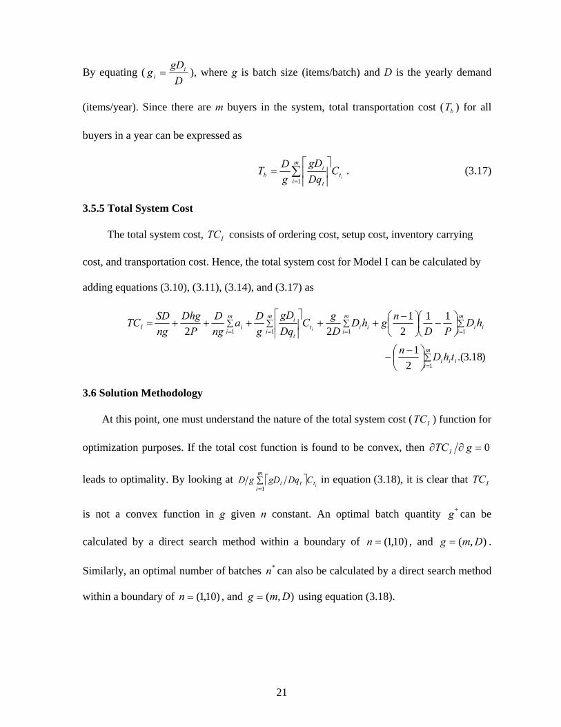
3.5.5 Total System Cost

The total system cost, consists of ordering cost, setup cost, inventory carrying

cost, and transportation cost. Hence, the total system cost for Model I can be calculated by

adding equations (3.10), (3.11), (3.14), and (3.17) as

ITC

)18.3.(

21

112

122

1

1 111

∑

∑ ∑∑∑

=

= ===

⎟⎠⎞

⎜⎝⎛ −

−

⎟⎠⎞

⎜⎝⎛ −⎟⎠⎞

⎜⎝⎛ −

++⎥⎥

⎤⎢⎢

⎡+++=

m

iiii

m

i

m

iiiii

m

it

t

im

iiI

thDn

hDPD

nghDDgC

DqgD

gDa

ngD

PDhg

ngSDTC

i

3.6 Solution Methodology

At this point, one must understand the nature of the total system cost ( ) function for

optimization purposes. If the total cost function is found to be convex, then

ITC

0=∂∂ gTCI

leads to optimality. By looking at ⎡ ⎤∑=

m

itti i

CDqgDgD1

in equation (3.18), it is clear that

is not a convex function in g given n constant. An optimal batch quantity can be

calculated by a direct search method within a boundary of

ITC

*g

)10,1(=n , and .

Similarly, an optimal number of batches can also be calculated by a direct search method

within a boundary of , and

), D(= mg

*n

,(m)10,1(=n )Dg = using equation (3.18).

22

Example 3.1 Item shipped in equally-sized batches upon production completion

Assume, units/year, 1250 units/year, , 1900=P == ∑=

m

iiDD

190=S 3.1=h ,

. Data is given in Table 1. For integer n, the minimum total cost is presented in

Table 2. Necessary unit conversion is performed prior to solution. For detailed results, see

30=tq

Appendix. Figure 3.2, a plot using MatLab 2009b; the minimum total cost is marked on the

figure. In Figure 3.2, a sudden cut occurs in the plot because at that point the number of

vehicle required changes for some buyers.

Table 1: Data for single vendor 9 buyers problem

Buyer (days) ia iD ih it itC

1 9 150 1.9 4.0 50 2 14 230 1.2 2.0 40 3 13 180 2.8 2.5 40 4 21 114 1.3 7.0 50 5 20 185 1.5 6.0 60 6 27 80 2.2 14.0 100 7 12 45 2.6 19.0 100 8 16 145 2.8 5.0 50 9 10 121 1.7 9.0 60 SUM 142 1250

Table 2: Summary of results

N g ITC 1 608 3951.11 2 468 3870.08 3 468 3900.73 4 405 3981.31

23

1 1.5 2 2.5 3 3.5 4 4.5 5 5.5 6

448

458

468

478

488

498

3800

3900

4000

4100

4200

4300

4400

4500

TC1

n=2 g=468 TC 1=3870.08

g

n

Figure 3.2: Graphical representation of ITC

3.7 Sensitivity Analysis for Model I

The total cost is a solution of the model where model parameters (vendor holding

cost, setup cost, and production to total yearly demand ratio) are presumably fixed. It is

useful to carry out sensitivity analysis of the model. For this purpose, effect of changes in

system parameters must be verified to check if the current solution

1. Remains unchanged.

2. Becomes sub-optimal, etc.

24

3.7.1 Effect of S on ITC The vendor setup cost S plays a major role in determining total cost of the system,

and it also affects the optimal batch size and number of batches in a lot. The effect of S on

total system cost, is expressed mathematically in equation (3.19), ITC

ngD

STCI =∂∂ , (3.19)

which is a constant term. The rate and direction of change of with respect to S depend

on the values of parameters used in the numerical example. If we put values of D, n, and g

from Table 10 and Table 11 in equation (3.19), then we can observe that for unit change in

S, will increase by $0.93.

ITC

ITC

3.7.2 Effect of h on ITCThe vendor’s holding cost h is an important parameter in developing the model. The

effect of h on total system cost is expressed mathematically in equation (3.20), ITC

P

Dgh

TCI

2=

∂∂ , (3.20)

which is also a constant term. The rate and direction of change of with respect to h

depend on the values of parameters used in the numerical example. If we put values of D, n,

and g from Table 10 and Table 11 (presented later), then we can write, that for every unit

increase (decrease) in h, will increase (decrease) by $232.00.

ITC

ITC

3.7.3 Effect of P/D on ITCThe ratio between production rate and total yearly demand P/D is not only an

important parameter to determine the total cost; but also, in conjugation with the vendor

holding cost h, the ratio determines which model to choose for a particular scenario among

the three. The effect of P/D on total system cost, is expressed mathematically in

equation (3.21),

ITC

25

∑⎟⎞⎛+−=

∂ mI hD1g1hgTC. (3.21)

=⎠⎜⎝

−∂ 1i

ii22 2n

DAA2A

The effect of P/D over is represented by Figure 3.3 using equations (3.21)

and

ITC

[ ]5,0∈DP . A study is performed with respect to

of P

P/D where the parameter values are

the same except for the values /D, which changes from 1 to 5, and the results are

presented in Table 3. Figure 3.3 illustrates that P/D ratio affects ITC changes rapidly up to

2.1, and beyond this point, ITC becomes less sensitive to a change in P/D. We can also

write that ITC increases as the ratio increases. Table 3 summarizes the change in ITC for

the change in P/D ratio.

3.8 Model II: Items Are Shipped In Every Dg Period

As described abo Dg ve, a vendor holds items and ships them in every period. In

izes e equal and there are n batches in

a lot. F

the second model we are assuming all batch s in a lot ar

igure 3.4 shows the production and inventory flow for the second model. In Figure

3.1, PG , ii DG , and it , are the time segments, which represent the production time for a

batch including transportation time demand, consumption time for thi buyer and

trans ti e for i buyer, respectively. In Figure 3.4, triangle (MNO) represents the

ideal inventory for the vendor. The triangle (ABC) represents the ideal inventory for the

thi buyer when the item is received at the end of previous inventory. The area (XYZ)

represents the inventory built up in the vendor’s warehouse due to constant production of

ms.

porta on tim

ite

th

26

Table 3: Effect of P/D (= A) ratio on

A

ITC

1.0 404.75 1.5 179.89 2.0 101.19 2.5 64.76 3.0 44.97 3.5 33.04 4.0 25.30 4.5 19.99 5.0 16.19

0

50

100

150

200

250

300

350

400

450

0 0.5 1 1.5 2 2.5 3 3.5 4 4.5 5 5.5

ATCI

∂∂

Figure 3.3: Effect of P/D (= A) ratio on ITC

ATCI

∂∂

A

27

it P A

Figure 3.4: Inventory flow in Model II

In the beginning of the cycle, the vendor starts production at a finite rate and

inventory builds up at a constant rate. In Figure 3.4, the slope MO is the rate of

accumulating inventory during production. As soon as production of the first batch is

complete, items are shipped to each buyer, and inventory of vendor is depleted. At this

point, the vendor begins producing the next batch. Since we assumed to avoid

shortage, inventory begins building up for the vendor beyond G as , as shown

in Figure 3.4. When a buyer’s inventory drops to transportation time demand, new items are

shipped, and the vendor’s inventory is reduced by G. This process is repeated until the entire

lot is produced. Items are shipped to all buyers at the same time, but buyers will receive

items after time since shipping time for each buyer varies. Items are readily available to

consume as soon as the buyer receives them, and the buyer consumes the items at a constant

rate. In Figure 3.4, slope AC is the consumption rate. Since buyer consumes items in a

DP >

DG /PG / <

it

B C

M N

O

Q

X S

P

Q

R

Y

Z

T

)(PG

Dg−G/P

BU

YER

i

i

DG

NEW LOT

TIME

BA

TCH

SIZ

E

VEN

DO

R

28

constant rate, on-hand inventory begins decreasing constantly. When the new items arrive,

inventory drops to zero. Hence, they buyer does not have to hold new items for extra time,

unlike the first model.

Notice that the cycle propels the time so that new items in the vendor’s warehouse

multiply. Since the production is continuous until the entire lot is produced, the inventory

level also rises with time. Figure 3.4 proves this notion with the area of triangle (QRS),

which is double that of triangle (XYZ).


This section derives the average inventory in Model II for the entire supply chain

system containing a single vendor and multiple buyers. Again, the demand is deterministic

and prohibits backlog and shortage; the production rate is presumably greater than the

demand rate to avoid shortage. The total system inventory consists of buyer’s inventory, and

vendor’s inventory, . mI


Each buyer receives amount of item in each shipment and takes iG ii DG amount of

time to consume. So each buyer’s average inventory for the first batch is ( ii DG 22 ). If

there are n batches in a lot, average inventory, , for buyer per cycle can be expressed

as,

ibI thi

i

ib D

GnIi

2

2= . (3.22)

We determine that iiii dtDDgG += , and upon substituting in Equation (3.22) and

simplifying, we obtain

29

⎟⎟⎠

⎞⎜⎜⎝

⎛++=

i

iiiiib D

dtDdt

gDD

gnIi

22

22 2

2. (3.23)

Since there are ngD number of cycles per year, then the average inventory, per year

can be expressed as

yeariI

⎟⎟⎠

⎞⎜⎜⎝

⎛++=

i

iiiiii D

dtDdt

gDD

gnnGDI

year

22

22 2

2. (3.24)

We determine , so substituting ( ii dtGg −= ) g in Equation (3.24), we get,

⎥⎥⎦

⎤

⎢⎢⎣

⎡+−+−=

i

iiiiii

iiii D

dtDdt

dtGDD

dtGGDI

year

22

22 )(2)(

2. (3.25)

Upon simplification this results in,

⎭⎬⎫

⎩⎨⎧

+−+⎭⎬⎫

⎩⎨⎧ −+=

i

iii

iii

ii GD

DGDG

Ddt

DD

dtGD

DI

year 21

21

222 , (3.26)

Therefore, average inventory, for all (m buyers) buyers per year can be expressed as bI

∑∑∑=== ⎭

⎬⎫

⎩⎨⎧

+−+⎭⎬⎫

⎩⎨⎧ −+=

m

i i

iii

m

i

iii

m

iib D

DDD

dtGD

DdtD

DGI

1

22

112

211

2. (3.27)


The vendor produces items in batches at a finite rate and holds them until the

production of the first batch is finished, and then, he ships in every g/D period. Remember,

to save on ordering cost, buyers only place order in the beginning of the lot and every batch

is automatically shipped after a g/D period. If each batch size is G and requires G/P periods

to produce, the average inventory during the first batch is PG 22 . Since the second batch is

shipped after it was produced, the vendor holds this batch for )( PGDg − period of time.

Therefore, the average inventory during the second batch is [ )(22 PGDgGPG −+ ]. The

third shipment also remains for a while before it is shipped and actually remains relatively

30

longer (twice) than the second batch. In Figure 3.4, we can see that QS is double YZ, which

represents the times that previous batches are remaining in the warehouse. This continues to

occur until the entire lot is exhausted. If there are n batches in a lot, the nth batch will have to

remain in warehouse for ))(1( PGDgn −− amount of time. Therefore, the total average

inventory for the vendor, per cycle, can be expressed as

( ){ 1...32121 2

−++++⎟⎠⎞

⎜⎝⎛ −+= nG

PG

Dg

PnGI

cyclev }. (3.28)

If each batch size is G and there are n batches in a lot, then in a complete cycle, nG

amount of items are produced. So, the total number of cycles in a year is ngD . Therefore,

average inventory for the vendor per year can be expressed as

( ){ } '

2

1...32121

QDnG

PG

Dg

PnGIv ⎥

⎦

⎤⎢⎣

⎡−++++⎟

⎠⎞

⎜⎝⎛ −+= , (3.29)

where the lot size . We define , by substitution expression nGQ =' ∑=

+=m

iii dtgG

1g in

terms of , so G

( ){ }⎥⎥⎥⎥

⎦

⎤

⎢⎢⎢⎢

⎣

⎡

−++++⎟⎟⎟⎟

⎠

⎞

⎜⎜⎜⎜

⎝

⎛

−−

+=∑= 1...321

21

2

nGPG

D

dtG

PGn

nGDI

m

iii

v , (3.30)

this, after simplification, yields

( ) ( ) ( )P

DGndtnGnP

DGIm

iiiv 2

12

121

2 1

−−

−−

−+= ∑

=. (3.31)


In an integrated supply chain system the total average inventory is calculated by

adding average yearly inventories for all buyers using equation (3.27) and vendor equation

(3.31). Therefore, the yearly average inventory of the system can be written as follows:

31

( ) .2

1

22

211

2

1

1

22

11

⎭⎬⎫

⎩⎨⎧ −−

−+

+⎭⎬⎫

⎩⎨⎧

+−+⎭⎬⎫

⎩⎨⎧ −+=

∑

∑∑∑

=

===

PDGdtGn

PDG

DD

DD

dtGD

DdtD

DGI

m

iii

m

i i

iii

m

i

iii

m

ii

(3.32)

3.9 Total Cost for Model II

In the current and previous sections, inventories for the vendor and all of the buyers

are calculated under assumptions of the second model. Usually, the total cost of the system

consists of the major costs, such as (a) ordering cost, (b) setup cost, (c) inventory holding

cost, and (d) transportation cost. The total system cost consisting of these four elements can

be calculated.

3.9.1 Ordering Cost

Each time a buyer places an order with the vendor, he incurs a cost, which may be

related to paperwork, telephone calls, etc. We assume each buyer places an order before the

cycle starts. Hence, each buyer will place nGD number of orders in a year. Therefore,

buyers in a year will place

m

nGDm number of orders. The cost of placing one order for the

ith buyer is . Therefore, total ordering cost A for all buyers can be expressed as ia

∑=

=m

iia

nGDA

1, (3.33)

where D is the demand rate (units/year), n is the number of batches in a lot and G is batch

size.

3.9.2 Setup Cost

Each time the vendor starts a new lot, production requires a setup such as changing

die, setting raw materials, etc. If the manufacturing process requires setup for every new lot,

then the total number of setup required is nGD . Thus, the total setup cost ( ) can be

calculated as

mS

32

nGSDSm = , (3.34)

where D is the demand rate (units/year), n is the number of batches in a cycle, G is batch

size, and S is setup cost per lot.


While the batch is being produced, inventory builds up. Thus, the vendor incurs the

inventory carrying cost until production is complete and items are shipped. Similarly, each

buyer receives items and holds them until all of the items are consumed. Therefore, each

buyer also incurs the item carrying cost, and the total system inventory carrying cost can be

calculated.


From equation (3.27) we know the average yearly inventory for all buyers. If is the

carrying cost for ith buyer, inventory holding cost for all buyers per year can be calculated as

ih

∑∑∑=== ⎭

⎬⎫

⎩⎨⎧

+−+⎭⎬⎫

⎩⎨⎧ −+=

m

i i

iiii

m

i

iiii

m

iiib D

DDD

hdtGD

DhdthD

DGH

1

22

112

211

2, (3.35)

where is the yearly demand of ith buyer, G is batch size, D is demand rate (units/year), n

is number of batches in a lot, and P is production capacity (units/year).

iD


From equation (3.31) we know the average yearly inventory for the vendor. If is

the carrying cost for vendor, inventory holding cost ( ) for the vendor per year can be

h

mh

calculated as

PDGhndthnGhn

PDGhI

m

iiiv 2

)1(2

)1(2

)1(2 1

−−

−−

−+= ∑

=. (3.36)

33


Total system’s carrying cost consists of the buyer’s carrying cost per year and

vendor’s carrying cost. Equations (3.35) and (3.36) represent all buyers’ carrying cost and

vendor’s carrying cost, respectively. Hence, the total system’s carrying cost H can be

expressed as

.2

)1(2

2211

2

1

1

22

11

⎭⎬⎫

⎩⎨⎧ −−

−++

⎭⎬⎫

⎩⎨⎧

+−+⎭⎬⎫

⎩⎨⎧ −+=

∑

∑∑∑

=

===

PDGdtGhn

PDGh

DD

DD

hdtGD

DhdthD

DGH

m

iii

m

i i

iiii

m

i

iiii

m

iii

(3.37)


Every time the vendor sends a shipment to a buyer, the buyer incurs transportation

cost. In reality, the capacity of a transportation vehicle is limited. Again, even if a vehicle is

partially filled, the buyer has to pay the entire price of full load. Another factor is

transportation cost for one shipment can be different among buyers depending on their

distances from the vendor. If is the carrying capacity of a vehicle and is the shipment

size, the receiving buyer has to pay for

tq ig

ti qG number of vehicles. If the cost/vehicle is

for ith buyer, and there are n number of batches in a cycle, then, transportation cost per

cycle ( ) to the ith buyer can be calculate as,

itC

icycleT

ii t

t

icycle C

qG

nT ⎥⎥

⎤⎢⎢

⎡= . (3.38)

Since there are ngD number of cycles in a year, transportation cost to buyer per year

can be calculated as,

thi

iii t

t

it

t

iyear C

DqGD

GDC

qG

nnGDT ⎥

⎥

⎤⎢⎢

⎡=⎥

⎥

⎤⎢⎢

⎡= . (3.39)

34

Equating D

GDG i

i = , where G is batch size (items/batch) and D is yearly demand

(items/year). Since there are m buyers in the system, total transportation cost T for all

buyers in a year can be expressed as

∑=

⎥⎥

⎤⎢⎢

⎡=

m

it

t

ii

CDqGD

GDT

1. (3.40)


The total system cost , consists of ordering cost, setup cost, inventory carrying



IITC

.2

)1(2

221

12

11

22

1111

⎭⎬⎫

⎩⎨⎧ −−

−++

⎭⎬⎫

⎩⎨⎧

+−+

⎭⎬⎫

⎩⎨⎧ −++⎥

⎥

⎤⎢⎢

⎡++=

∑∑

∑∑∑∑

==

====

PDGdtGhn

PDGh

DD

DD

hdtG

DD

hdthDD

GCDqGD

GD

nGSDa

nGDTC

m

iii

m

i i

iiii

m

i

iiii

m

iii

m

it

t

im

iiII i

(3.41)


At this point, it is necessary to understand the nature of the total system cost

function for optimization purposes. If the total function is convex, then,

IITC

IITC

0=∂∂ gTCII , which allows for optimality and optimal batch quantity evaluation. *g

By looking at ⎡ ⎤∑=

m

itti i

CDqGDGD1

in equation (3.41), it is clear that is not a

convex function in g given n remains constant. An optimal batch quantity can be


IITC

*g

)10,1(=n and .

Similarly, an optimal number of batches can also be calculated by a direct search method

within a boundary of and

), Dm(g =

*n

,(m)10,1(=n )Dg = using equation (3.41).

35

Example 3.2 Order shipped after every g/D period

Assume, units/year, 1300 units/year, S = $150, h = 2.1, and

. Data is given in Table 4. For integer n, the minimum total cost is $3727.11 (for n

= 2, and g = 506), presented in Table 4. Necessary unit conversion is performed prior in to

solution. For detailed result see Appendix. In Figure 3.5, a sudden cut occurs in the plot

because at that point the number of vehicle required changes for some buyers.

2300=P == ∑=

m

iiDD

1

40=tq



1 15 170 1.9 6.0 50 2 11 250 1.1 2.0 40 3 18 175 2.9 2.8 40 4 19 115 1.3 5.7 50 5 23 190 1.7 7.2 60 6 24 70 2.2 16.3 100 7 13.5 50 2.9 17.1 100 8 17.3 150 2.6 6.2 50 9 11.6 130 1.7 7.0 60 152.4 1300


n g IITC 1 647 3841.33 2 506 3727.11 3 506 3806.98 4 506 3948.97 5 233 4075.77 6 233 4111.09

3.11 Sensitivity Analysis for Model II

Sensitivity analysis has been performed in this section to test the robustness of the

proposed model, which is subject to change in given parameters, setup cost, vendor holding

cost, and production to demand ratio.

36

3.11.1 Effect of S on IITC

The vendor setup cost plays a major role in determining total cost of the

system, and it also affects the optimal batch size. So, it is important to understand the effect

of change in S on . The effect of S on total system cost is expressed in equation

(3.42),

IITC IITC

nGD

STCII =∂

∂ , (3.42)

which is a positive constant term. It can be written that increases (decreases)

with an increase (decrease) in setup cost S. If we implement values of D, n and g from Table

10 and Table 11 (shown later) for a unit change in S, then will increase by $1.11.

IITC

IITC

1 1.5 2 2.5 3 3.5 4 4.5 5 5.5 6486

496

506

516

526

536

3800

3900

4000

4100

4200

4300

4400

4500

4600

n=2 g=506 TC 2= 3727.11

TC

2

g

n

Figure 3.5: Graphical representation of TC II

37

3.11.2 Effect of h on IITC

The vendor’s holding cost is an important parameter in determining the total cost.

Also, to an extent, the vendor’s holding cost governs which model should be chosen among

the three presented.

It is important to understand how vendor holding cost h affects . The effect of h on

total system cost is expressed in equation (3.43),

IITC

IITC

⎭⎬⎫

⎩⎨⎧ −−

−+=

∂∂

∑= P

DGdtGnP

DGh

TC m

iii

II

12)1(

2, (3.43)

which is also a positive, constant term. It can be written that increases (decreases) with

an increase (decrease) in holding cost h. By inserting values of D, n, P, and G from Table 10

and Table 11 (shown later), there will be a unit change in h and will increase by $257.

IITC

TCII

3.11.3 Effect of P/D on IITC

The ratio between production rate and total yearly demand not only determines the

total cost, but also, it determines, in conjugation with vendor holding cost, which model to

choose for a particular scenario among the three presented. Hence, it is crucial to understand

the effect of P/D on total system cost . The effect of P/D on total system cost , is

expressed in equation (3.44).

IITC IITC

22II

AG

2h)1n(

A2Gh

ATC −

+−=∂

∂. (3.44)

The effect of P/D over is represented by Figure 3.6 using equations (3.44) and IITC

[ ]5,1∈DP . A study is performed with respect to P/D where the parameter values are the

same except for the values of P/D, which shifts from 1 to 5; the results are presented in

Table 6. Figure 3.6 reveals that P/D ratio affects and changes rapidly up to 2.0. IITC

38

Beyond this point, becomes less sensitive to change in P/D. We can also write that

increases as the ratio decreases. Table 6 summarizes the change in for the change

in P/D ratio.

IITC

IITC IITC

3.12 Model III: Items Shipped in Unequal Batches

As described above, the vendor holds items until the order is placed and then ships

items to buyers. In the third model, we assume that batch sizes in a lot are unequal, that they

increase by a factor k (where DPk = ) and that there are n batches in a lot. Figure 3.7

shows the production and inventory for the third model. A lot is produced with batch sizes

of …, . In Figure 3.7, ,1

⎟⎠⎞+ ∑

=

m

iiidtg ,dt

m

1iii ⎟⎠

⎞∑=

kg⎜⎝

⎛ +⎜⎝⎛ ,

1

2 ⎟⎠⎞

⎜⎝⎛ + ∑

=

m

iiidtgk ⎜

⎝⎛ + ∑

=

−m

iii

n dtgk1

1

P)dt

⎟⎠⎞

m

1iii∑

=, iig( + ii dtg +

thi

D)(

thi

, and , are the time segments, which represent the batch

production time, including transportation time demand, consumption time for buyer and

transportation time for buyer, respectively. In Figure 3.7, triangles MNO, OPQ and QRS

represent inventories for the vendor for subsequent batches. Triangles ABC, CDE and EFH

represent inventories for the buyer when the item is received immediately at the end of

previous inventory. In the beginning of the cycle, the vendor begins production at a finite

rate and inventory builds up at a constant rate. In Figure 3.7 the slope MN is the rate of

inventory build-up during production. As soon as production of the first batch

is complete, items are shipped to each buyer, and vendor inventory reduces to zero. At this

point, the vendor begins producing the next batch of size . Remember, we

assumed

it

thi

⎜⎝⎛ g ⎟

⎠⎞+ ∑

=

m

iiidt

1

⎟⎠⎞

id⎜⎝⎛ + ∑

=

m

iitkg

1

DP > to avoid shortage. Unlike the first two models, the third model’s batch size

increases with a multiplication factor of k. Hence, to avoid shortage,

39

A

Figure 3.6: Effect of P/D (= A) ratio on IITC

Table 6: Effect of P/D (= A) ratio on IITC

A

1.0 412.33 1.5 183.26 2.0 103.08 2.5 65.97 3.0 45.81 3.5 33.66 4.0 25.77 4.5 20.36 5.0 16.49

DdtgkPdtgkm

iii

nm

iii

n //1

1

1⎟⎠⎞

⎜⎝⎛ +=⎟

⎠⎞

⎜⎝⎛ + ∑∑

=

−

=. When the buyer’s inventory falls to the

transportation time demand, new items are shipped, and the vendor’s inventory is reduced to

zero. This is repeated until the entire lot is produced. Items are shipped to all buyers at the

same time, but buyers will receive items after time since shipping times vary among it

ATCII

∂∂

40

buyers. Items are readily available to consume as soon as the buyer receives them, and

buyer consumes the items at a constant rate. In Figure 3.7, slope BC is the consumption rate.

Since the buyer consumes items at a constant rate, on-hand inventory begins to decrease

constantly. When the new items arrive, inventory drops to zero. Hence, the buyer is not

required to hold new items for extra time, unlike the first model. Unlike the other two

models, in this model, neither the vendor nor the buyers need to hold a new batch in its

warehouse while the previous batch is being consumed.


This section derives the average inventory in Model III for the entire supply chain

system containing a single vendor and multiple buyers. Similar to the other two models, the

demand is deterministic and no backlog or shortage is allowed, the production rate has to be

greater than the demand rate. The total system inventory consists of buyer’s inventory

and vendor’s inventory .

bI

mI


Each buyer receives amount of items for the first shipment, followed by

, , …, items. Each buyer takes

iii dtg +

in gk +−1

iii dtkg + iii dtgk +2iidt ( ) iiii

n Ddtgk +−1 time to

consume the batch fully so each buyer’s average inventory for the first batch is

( ) iiii dtg + D22 . For the second batch, the average inventory is ( ) iiii Ddtkg 22+ ).

Similarly, for the batch, the average inventory is thn ( ) iiiin Ddtgk 221 +− . If there are n

batches in a lot, the average inventory ( ) for buyer per cycle can be expressed as ibI thi

[ ].)(...)()()(2

1 212222iii

niiiiiiiii

ib dtgkdtgkdtkgdtg

DI

i++++++++= − . (3.45)

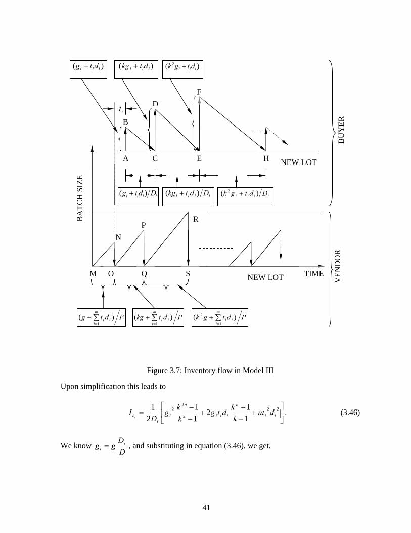
41

Figure 3.7: Inventory flow in Model III

Upon simplification this leads to

⎥⎦

⎤⎢⎣

⎡+

−−

+−−

= 222

22

112

11

21

ii

n

iii

n

ii

b dntk

kdtgkkg

DI

i. (3.46)

We know DD

gg ii = , and substituting in equation (3.46), we get,

BU

YER

it

A

B

C

D

E

F

H

M

N

O

P

Q

R

S TIME

BA

TCH

SIZ

E

)( iii dtg + )( iii dtkg + )2iii dtgk + (

iiii Ddtg )( + iiii Ddtkg )( + iiii Ddtgk )( 2 +

Pdtgm

iii )(

1∑=

+ Pdtkgm

iii )(

1∑=

+ Pdtgkm

iii )(

1

2 ∑=

+

VEN

DO

R

NEW LOT

NEW LOT

42

⎥⎥⎦

⎤

⎢⎢⎣

⎡+

−−

+−−

= 222

2

2

22 2

11

11

21

iiiii

nni

ib dntdt

DD

gk

kkk

DD

gD

Ii

. (3.47)

Assume the sum of all batches in a lot equals , so the lot size is 'Q

Gk

kQn

11'

−−

= . (3.48)

Therefore, there will be number of lots in a year. Hence, the average inventory

for buyer per year can be expressed as

'/ QDyeariI

thi

⎥⎦

⎤⎢⎣

⎡+

−−

+−−

= 222

2

2

22

' 211

11

21

iiiii

nni

ii dntdt

DDg

kk

kk

DDg

DQDI

year. (3.49)

If there are m buyers in the system, the average inventory for all buyers per year can be

expressed as

⎥⎦

⎤⎢⎣

⎡+

−−

+−−

= ∑∑∑===

m

i i

iim

iii

nn

ii

n

b Ddtndt

Dg

kkD

kk

Dg

QDI

1

22

112

2

2

2

'

211

11

21 . (3.50)


The vendor produces batch items at a finite rate with a batch of sizes ,

, , ..., . The vendor holds items until

production is finished and ships as soon as the batch production is completed. Since batch

sizes are unequal, we can calculate the work-in-process (WIP) inventory for the vendor.

Hence, the WIP inventory per cycle can be expressed as:

⎟⎠⎞

⎜⎝⎛ + ∑

=

m

iiidtg

1

⎟⎠⎞

⎜⎝⎛ + ∑

=

m

iiidtkg

1⎟⎠⎞

⎜⎝⎛ + ∑

=

m

iiidtgk

1

2 ⎟⎠⎞

⎜⎝⎛ + ∑

=

−m

iii

n dtgk1

1

P

dtgk

P

dtgk

P

dtkg

P

dtgWIP

m

iii

nm

iii

m

iii

m

iii

cycle 2...

222

2

1

)1(2

1

22

1

2

1⎟⎠⎞

⎜⎝⎛ +

++⎟⎠⎞

⎜⎝⎛ +

+⎟⎠⎞

⎜⎝⎛ +

+⎟⎠⎞

⎜⎝⎛ +

=∑∑∑∑=

−

=== . (3.51)

43

If the lot size is and there are number of cycles in a year, the average WIP

inventory (WIP ) per year can be expressed as

'Q

year

'/ QD

⎥⎦

⎤⎢⎣

⎡+

−−

+−−

= ∑∑==

m

iii

m

iii

nn

year dtndtgkk

kkg

PQDWIP

1

22

12

22

' 211

11

21 , (3.52)

Where P/D = k, D is yearly demand (item/year), g is the minimum batch size, n is number

of batches in a lot, is lot size (item/lot) and P is production rate (item/year). 'Q


In an integrated supply chain system, the total average inventory is calculated by

adding average yearly inventories of all buyers and vendors using equations (3.50) and

(3.52). Therefore, yearly average inventory I of the system can be written as

⎥⎥⎥⎥⎥

⎦

⎤

⎢⎢⎢⎢⎢

⎣

⎡

⎭⎬⎫

⎩⎨⎧

+−−

+−−

+

⎪⎭

⎪⎬⎫

⎪⎩

⎪⎨⎧

++⎟⎟⎠

⎞⎜⎜⎝

⎛−−

=

∑∑

∑∑∑

==

===

m

iii

m

iii

nn

m

i i

iim

iii

m

i i

n

dtndtgk

kkkg

P

Ddt

dtD

gDDg

kk

QDI

1

22

12

22

1

22

112

2

2

2

'

211

111

1211

2. (3.53)

3.13 Total Cost for Model III

In the current and previous sections, inventories for the vendor and all buyers are

calculated as in the second model. Usually, the total cost of the system consists of major

costs: (a) ordering cost, (b) setup cost, (c) inventory holding cost, and (d) transportation

cost. The total system cost consisting of these costs can be calculated.

3.13.1 Ordering Cost

Each time a buyer places an order to the vendor, the buyer incurs a cost, which may

consist of paperwork, telephone calls, etc. Assume each buyer places an order before the

cycle starts. Hence, each buyer will place number of orders in a year. Therefore,

buyers in a year will place number of orders. The cost of placing one order for ith

'/ QD m

'/ QmD

44

buyer is . Therefore, total ordering cost A for all buyers can be expressed as ia

∑=

=m

iia

QDA

1' , (3.54)

where D is the demand rate (units/year), n is the number of batches in a cycle, and is lot

size (items/lot).

'Q

3.13.2 Setup Cost

Each time the vendor begins production of a new lot, he incurs a setup cost for

changing die, setting raw materials, etc. If the manufacturing process requires setup for

every new lot, the total number of setup requires is . Hence, the total setup cost

can be calculated as,

'/ QD mS

'QSDSm = , (3.55)

where D is the demand rate (units/year), n is the number of batches in a cycle, is lot size

(items/lot) and S setup cost per lot ($/lot).

'Q


While the batch is being produced, inventory builds up. Thus, the vendor incurs an

inventory carrying cost until production is completed, and he then ships the items. Similarly,

each buyer receives items, holding them until all items are consumed. Therefore, each buyer

also incurs a carrying cost. The total system inventory carrying cost can be calculated.


From equation (3.50), we know the average yearly inventory for all buyers. If is

the carrying cost for ith buyer, then inventory holding cost for all buyers per year

ih

bh

can be calculated as

45

⎥⎦

⎤⎢⎣

⎡+

−−

+−−

= ∑∑∑===

m

i i

iiim

iiii

nn

iii

n

b Dhdtnhdt

Dg

kkhD

kk

Dg

QDh

1

22

112

2

2

2

'

211

11

21 , (3.56)

where is the yearly demand of ith buyer, g is batch size, D is demand rate (units/year), n

is number of batches in a lot and P is production capacity (units/year).

iD


From equation (3.52), we know the average yearly inventory for the vendor. If is

the carrying cost for the vendor, then inventory holding cost for the vendor per year can

be calculated as follows:

h

vh

⎥⎦

⎤⎢⎣

⎡+

−−

+−−

= ∑∑==

m

iii

m

iii

nn

v dtndtgkk

kkg

Ph

QDh

1

22

12

22

' 211

11

2. (3.57)


Total system’s carrying cost consists of the buyer’s carrying cost per year and the

vendor’s carrying cost. Equations (3.56) and (3.57) represent the carrying costs for all of the

buyers as well as for the vendor, respectively. Hence, the total system’s carrying cost H can

be expressed as

⎥⎥⎥⎥⎥

⎦

⎤

⎢⎢⎢⎢⎢

⎣

⎡

⎪⎭

⎪⎬⎫

⎪⎩

⎪⎨⎧

++

⎭⎬⎫

⎩⎨⎧ +

−−

+⎭⎬⎫

⎩⎨⎧ +

−−

=

∑∑

∑∑∑

==

===

m

i i

iiim

iii

m

iiii

m

iii

nn

iii

n

Dhdt

dtPhn

hdtD

dtPh

kkghD

DPh

kkg

QDH

1

22

1

22

11122

22

'

11121

11

2. (3.58)


Every time the vendor sends a shipment to a buyer, the buyer incurs transportation

cost. In reality, capacity of a transportation vehicle is limited. Again, even if a vehicle is

partially filled, the buyer has to pay according to the full-load price. Another thing to

consider is the transportation cost for one shipment because it may vary among different

buyers depending on their distances from the vendor. If is carrying capacity of a vehicle tq

46

and ( )iiin dtgk +−1 is the shipment size, then the receiving buyer has to pay for

( ) tiiin qdtgk +−1 number of vehicles. If the cost of a vehicle is for ith buyer, and there

are n number of batches in a cycle, then the transportation cost per cycle paid by ith

buyer, can be calculate as

itC

cycleiT

icycle t

n

j t

iiij

i Cq

dtgkT ∑

=

−

⎥⎥

⎤⎢⎢

⎡ +=

1

1

, (3.59)

since there are ( 'QD ) number of cycles in a year, transportation cost to buyer per

year can be calculated as

yeariT thi

iyear t

n

j t

iiij

i Cq

dtgkQDT ∑

=

−

⎥⎥

⎤⎢⎢

⎡ +=

1

1

' , and (3.60)

Since there are m buyers in the system, the total transportation cost for all buyers in a

year can be expressed as follows

yearT

∑∑= =

−

⎥⎥⎥

⎥

⎤

⎢⎢⎢

⎢

⎡ +=

m

it

n

j t

iiij

year iC

q

dtDDgk

QDT

1 1

1

' . (3.61)


The total system cost consists of ordering cost, setup cost, inventory carrying



IIITC

.

11121

11

2

1 1

1

''1'

1

22

1

22ii dt

11122

22

'

∑ ∑∑

∑∑∑∑∑

= =

−

=

=====

⎥⎥⎥⎥

⎥

⎤

⎢⎢⎢⎢

⎢

⎡+

+++

⎥⎥⎦

⎤

⎢⎢⎣

⎡

⎪⎭

⎪⎬⎫

⎪⎩

⎪⎨⎧

+⎩⎨⎧ +

−−

+⎭⎬⎫

⎩⎨⎧ +

−−

=

m

it

n

j t

iiij

m

ii

m

i i

iiim

i

m

iii

m

iii

nn

iii

n

III

iC

q

dtDD

gk

QD

QSDa

QD

Dhdt

Phndt

Ddt

Ph

kkghD

DPh

kkg

QDTC +

⎭⎬⎫

ih

(3.62)

47


At this point, we need to understand the nature of the total system cost

function for optimization purposes. If the total function is convex, then

IIITC

IIITC

0=∂∂ gTCIII leads to optimality, and the optimal batch quantity can be evaluated. *g

By looking at ( )⎡∑ ∑= =

− +m

i

n

jttiii

ji

CqdtDgDkQD1 1

1' / ⎤ in equation (3.62), it is clear that

is not a convex function in g given n constant. An optimal batch quantity can be


IIITC *g

)10,1(=n , and .

Similarly an optimal number of batches can also be calculated by a direct search method

within a boundary of , and

), Dmg (=

*n

(m)10,1(=n ), Dg = using equation (3.62).

Example 3.3 Unequal size batches are shipped.

Assume, units/year, 1400 units/year, , , and

. Data is given in Table 7. For integer n, the minimum total cost is $2552.67 (for

, and ), and a summary of results are presented in Table 8. Necessary unit

conversion is performed prior to solution. For detailed results see Appendix. In Figure 3.2, a

sudden cut occurs in the plot because at that point the number of vehicle required changes

for some buyers.

2200=P

137

== ∑=

m

iiDD

1

160=S 1.1=h

25=tq

7=n =g

3.15 Sensitivity Analysis for Model III

Sensitivity analysis has been performed in this section to test the robustness of the

proposed model, which is subject to change in the following areas: given parameters, setup

cost, vendor holding cost and production to demand ratio.

48



1 12 160 2.1 6.0 50 2 14 310 1.0 2.0 40 3 16 170 2.8 4.0 40 4 18 120 1.4 5.0 50 5 17 187 1.7 7.4 60 6 23 72 1.9 13.8 100 7 15 60 2.7 17.8 100 8 19 175 2.3 5.9 50 9 11 146 1.9 8.3 60 145 1400


n g IIITC 1 633 5032.51 2 414 4776.54 3 137 4331.17 4 137 3584.15 5 137 3057.53 6 137 2714.58 7 137 2552.67 8 127 2582.08 9 94 3495.29

10 63 4140.88

3.15.1 Effect of S on IIITC

The vendor setup cost plays a major role in determining total cost of the system, and

it also affects the optimal batch sizes. So, it is important to understand the effect of change

in S on . The effect of S on total system cost is expressed in equation (3.63), IIITC IIITC

'QD

STCIII =∂

∂ , (3.63)

which is a positive, constant term. It can be written that TC increases (decreases) with

increase (decrease) in setup cost S. If we apply the values of D, n and g from Table 10 and

Table 11 (shown later), then, for unit change in S, TC will increase by $0.49.

III

III

49

3.15.2 Effect of h on IIITC

The vendor’s holding cost is an important parameter in determining total cost.

Vendor’s holding cost also governs to an extent which model should be chosen among three

presented here. So, an understanding of how a change in vendor holding cost h affects IIITC

4 5 6 7 8 9 10117

127

137

147

157

167

2500

3000

3500

4000

4500

5000

5500

6000

6500

7000

n=7 g=137 TC 3=2552.67

TC

3

g

n

Figure 3.8: Graphical representation of IIITC

is required. The effect of h on total system cost is expressed in equation (3.64), IIITC

∑∑==

+−−

+−−

=∂

∂ m

iii

m

iii

nnIII dt

Pndt

Pkkg

Pkkg

QD

hTC

1

22

12

22

'

11121

11

2, (3.64)

which is a positive, constant term. It can be written that TC increases (decreases) with

increase (decrease) in setup cost h. If we use values of D, n and g from Table 11 (shown

III

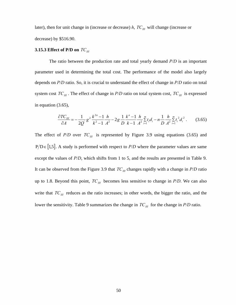
50

later), then for unit change in (increase or decrease) h, will change (increase or

decrease) by $516.90.

IIITC

3.15.3 Effect of P/D on IIITC

The ratio between the production rate and total yearly demand P/D is an important

parameter used in determining the total cost. The performance of the model also largely

depends on P/D ratio. So, it is crucial to understand the effect of change in P/D ratio on total

system cost . The effect of change in P/D ratio on total system cost, is expressed

in equation (3.65),

IIITC IIITC

∑=

−−−

−−−

−=∂

∂ m

iiiii

nnIII dt

Ah

Dndt

kk

Dg

Ah

kkg

QATC

1

22222

22

'

11

1211

21

]

∑=

m

iAh

12

1 . (3.65)

The effect of P/D over is represented by Figure 3.9 using equations (3.65) and IIITC

[ 5,1DP ∈ . A study is performed with respect to P/D where the parameter values are same

except the values of P/D, which shifts from 1 to 5, and the results are presented in Table 9.

It can be observed from the Figure 3.9 that changes rapidly with a change in P/D ratio

up to 1.8. Beyond this point, becomes less sensitive to change in P/D. We can also

write that reduces as the ratio increases; in other words, the bigger the ratio, and the

lower the sensitivity. Table 9 summarizes the change in for the change in P/D ratio.

IIITC

IIITC

IIITC

IIITC

51

III

Figure 3.9: Effect of P/D (= A) ratio on TC

A

-200

0 0 0.5 1

Table 9: Effect of P/D (= A) ratio on IIITC

A

1.0 -1590.45 1.5 -706.87 2.0 -397.61 2.5 -254.47 3.0 -176.72 3.5 -129.83 4.0 -99.40 4.5 -78.54 5.0 -63.62

-1800

-1600

-1400

-1200

-1000

-800

-600

-400

1.5 2 2.5 3 3.5 4 4.5 5 5.5

A TC III ∂

∂

ATC III

∂∂

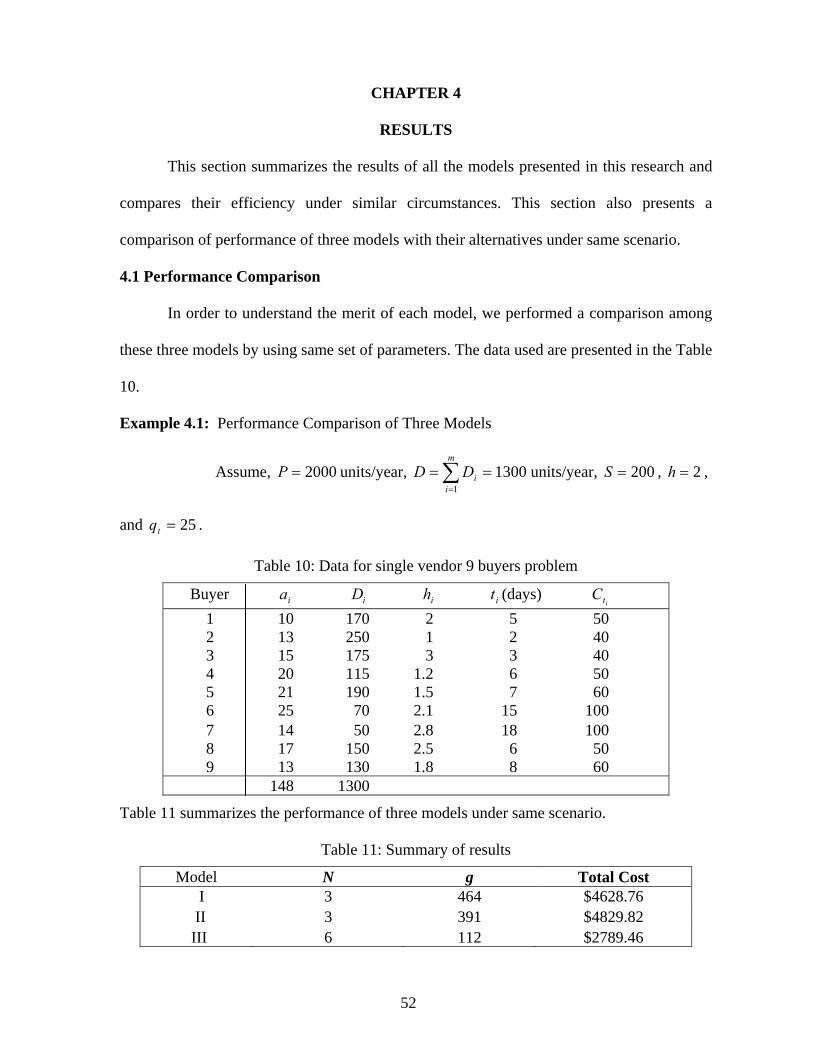
52

CHAPTER 4

RESULTS

This section summarizes the results of all the models presented in this research and

compares their efficiency under similar circumstances. This section also presents a

comparison of performance of three models with their alternatives under same scenario.

4.1 Performance Comparison

In order to understand the merit of each model, we performed a comparison among

these three models by using same set of parameters. The data used are presented in the Table

10.

Example 4.1: Performance Comparison of Three Models

Assume, units/year, 1300 units/year, , 2000=P == ∑=

m

iiDD

1

200=S 2=h ,

and . 25=tq



1 10 170 2 5 50 2 13 250 1 2 40 3 15 175 3 3 40 4 20 115 1.2 6 50 5 21 190 1.5 7 60 6 25 70 2.1 15 100 7 14 50 2.8 18 100 8 17 150 2.5 6 50 9 13 130 1.8 8 60 148 1300

Table 11 summarizes the performance of three models under same scenario.


Model N g Total Cost I 3 464 $4628.76 II 3 391 $4829.82 III 6 112 $2789.46

53

It is clear from Table 8 that Model III provides lower total cost than Model I and Model II

under same circumstances.

4.2 Comparison with Alternative Approach

In our original models, items are produced in batches noting that there are n batches

in a lot and that there can be multiple lots in a year. In an alternative approach, we verified

that when the items are transferred in lots instead of batches, we performed a comparative

study between two approaches to understand which one is more efficient. We used the same

data set (given in Table 10) as input and presented the summary of results in Table 12.

Table 12: Performance comparison with alternative models

Model I Model II Model IIIOriginal Model $4628.76 $4829.82 $2789.46

Alternative $4887.00 $5070.92 $2455.89

54

CHAPTER 5

RESEARCH SUMMARY AND CONCLUSIONS

This section summarizes the research and concludes the findings of the research.

This section also discusses the significance of this work and applicability of the research.

Finally, a few suggestions are made to provide direction for the future researcher.

5.1 Conclusions

This research describes three models to solve an integrated inventory problem where

a single vendor supplies a single product to multiple buyers. In the first and second model,

the vendor transfers items in equally-sized batches; in the third, however, the vendor

transfers items in unequally-sized batches. Each transfer of batches incurs transportation

cost. Optimum solution techniques for all three models are presented while sensitivity

analysis has also been performed.

This study does not restrict the vendor to have either greater or less holding cost than

everyone else in the system. The study is also flexible in accommodating unequal

transportation time and cost for each buyer in the system.

A numerical study performed on the three models presented here reveals that under

similar circumstances, the third model is always more efficient in solving the integrated

inventory system.

Through a set of numerical problems, we found that splitting lots does not always

produce better results. In some cases, alternate models, which do not split lots, produce

better results than the models that participate in splitting lots. However, an extensive review

is required to conclude whether or not models with no lot-splitting consistently produce

better results.

55

5.2 Research Significance

In the recent past, multiple researchers have investigated the integrated inventory

supply chain system and developed models for it. These studies are based on many ideal

variables such as perfect transportation system and equal carrying costs for vendor and

buyers in the system regardless of geographic location, which are unrealistic. This research,

however, refines the work of Hoque (2008) into a more realistic model. This research

presents an approach to obtain just-in-time delivery of products with an objective of

reducing the overall system cost. Models presented in this research allow different

transportation cost and time; also, they facilitate different ordering and holding costs for

vendors and buyers. This research also allows vendors to ship batches of equal or unequal

sizes and does not restrict shipping before the entire lot is produced. The results of this

research is to find an optimal batch size; input only includes basic information such as

holding cost, ordering cost, transportation capacity, transportation cost and yearly demand.

However, the storage capacity constraint for both the vendor and the buyers was not been

considered.

5.3 Possible Future Extensions

The inventory models presented here are subject to certain restrictions, which can be

considered in future research. By relaxing some of those restrictions, the problem will

become more complex but more realistic. However, in order to enhance the applicability and

model performance, the following extensions are suggested:

(a) Nondeterministic demand: In this study, the yearly demand for the system is

considered deterministic, but in reality, this may not always the case. However, if a non-

deterministic demand, rather than a deterministic demand, is considered for an integrated

supply chain system, the models presented here will be closer to reality.

56

(b) Storage capacity constraint: In this research, storage capacity for vendor and

buyers are considered to be unconstrained. Again, realistically, that might not be the case

especially because some buyers may be located where the demand is high but where a big

storage capacity is not feasible. Thus, storage capacity constraints should be examined in

future research.

57

BIBLIOGRAPHY

Affisco, J., Nasri, F., and Paknejad, M. (1991). Investing in setup cost reduction in the one-vendor and many identical purchasers joint economic lot size model. Proceedings of the Decision Science Institute, Miami, FL, pp. 2661-76.

Affisco, J., Paknejad, M., and Nasri, F. (1993). A comparison of alternative joint vendor-purchaser lot-sizing models. International Journal Production Research, 31(11), pp. 2661-76.

Affisco, J., Paknejad, M., and Nasri, F. (1988). Investing in the setup cost reduction in the joint economic lot size model. Proceedings of the Decision Sciences Institute, Phoenix, AZ, pp. 1126-29.

Banerjee, A. (1986). A joint economic lot size model for purchaser and vendor. Decision Sciences, 17(3), pp. 292-312.

Benerjee, A., and Kim, S. (1995). An integrated JIT inventory model. International Journal of Operation & Production Mangement, 15(9), pp. 237-244.

Chen, Z.X., and Sarker, B.R. (2009). Multi-vendor integrated procurement-production system under shared transportation and just-in-time delivery system. Journal of the Operation Research Society, 111, pp. 1-13.

Comeaux, E.J., and Sarker, B.R. (2005). Joint optimization of process improvement investments for supplier-buyer cooperative commerce. Journal of the Operation Research Society, 56, pp. 1310-1324.

Ertogal, K., Darwish, M., and Ben-Daya, M. (2007). production and shipment lot sizing in a vendor-buyer supply chain with transportation cost. European Journal of Oprational Research, 176(3), pp. 1592-1606.

Goyal, S. (1988). "A joint economic lot size model for purchase and vendor": A comment*. Decision Sciences, 19(1), pp. 236-241.

Goyal, S. (1995). A one-vendor multi-buyer integrated inventory model: A comment. European Journal of Operational Research, 82(1), pp. 209-210.

Goyal, S. (1976). An integrated inventory model for a single supplier-single customer problem. International Journal of Production Research, 15(1), pp. 107-111.

Goyal, S. K., and Nebebe, F. (2000). Determination of economic production-shipment policy for a single-vendor-single-buyer system. European Journal of Operational Research, 121(1), pp. 175-178.

Goyal, S. (2000). On improving the single vendor single buyer integrated production inventory model with a generalized policy. European Journal of Operational Research, 125(2), pp. 429-430.

58

Goyal, S., and G., S. (1992). The individually responsible and rational decision approach to economic lot sizes for one vendor and many purchasers: A comment*. Decision Sciences, 23(3), pp. 777-784.

Hill, R. M. (1999). The optimal production and shipment policy for the single-vendor single-buyer integrated production-inventory model. International Journal of Production Research, 17(3), pp. 2463-75.

Hill, R. M. (1997). The single-vendor single-buyer integrated production-inventory model with a generalised policy. European Journal of Operational Research, 97(3), pp. 493-499.

Hill, R., and Omar, M. (2006, February 15). Another look at the single-vendor single-buyer integrated production-inventory problem. International Joural of Production Research, 44(4), pp. 791-800.

Hoque, M. A., and Goyal, S. (2000). An optimal policy for a single-vendor single-buyer integrated productiion-inventory system with capacity constraint of the transport equipment. International Journal of Production Economics, 65(3), pp. 305-315.

Hoque, M. (2008). Synchronizaton in the single-vendor multi-buyer integrated inventory supply chain. European Journal of Operational Research, 188(3), pp. 811-825.

Joglekar, P., and Tharthare, S. (1990). The individually responsible and rational decision approach to economic lot sizes for one vendor and many purchasers. Decision Sciences, 21(3), pp. 492-506.

Kim, S., and Ha, D. (2003). A JIT lot-splitting for supply chain management: Enhancing buyer supplier linkage. International Journal of Production Economics, 86(1), pp. 1-10.

Lu, L. (1995). A one-vendor multi-buyer integrated inventory model. European Journal of Operational Research, 81(2), pp. 312-323.

Pan, J. C-H., and Yang, J-S. (2002). A study of an integrated inventory with controllable lead time. International Journal of Production Research, 40(5), pp. 1263-1273.

Siajadi, H., Ibrahim, R., and Lochert, P. (2006). A single-vendor multi-buyer inventory model with a multiple shipment policy. International Journal of Advanced Manufacturing Technology, 27(9-10), pp. 1030-37.

Viswanathan, S. (1998). Optimal strategy for the integrated vendor-buyer inventory model. Eurppean Journal of Operational Research, 105(1), pp. 38-42.

Viswanathan, S., and Piplani, R. (2001). Coordinating supply chain inventories through common replenishment epochs. European Journal of Operational Research, 129(2), pp. 277-286.

Yau, M., and Chiou, C. (2004). On a replenishment coordination model in an integrated supply chain with one vendor and multiple buyers. European Journal of Operation Research, 159(2), pp. 406-419.

59

Zhou, Y-W., and Wang, S-D. (2007). Optimal production and shipment model for a single-vendor-single buyer integrated system. European Journal of Operational Research, 180(1), pp. 309-328.

60

APPENDIX

This section presents computational results of three models.

1. Computational results for Model I

Table 13: Computational results in detail

n g TC n g TC n g TC 1 101 9818.18 2 101 8396.16 3 101 7931.24 201 5390.48 201 4715.49 201 4521.43 301 4661.31 301 4258.76 301 4177.37 401 4209.07 401 3959.43 401 3950.86 501 4341.99 468 3870.08 468 3900.73 601 3977.62 501 4197.31 501 4245.57 608 3951.11 601 913.87 601 4010.97 701 4113.38 701 4116.83 701 4258.18 801 4015.76 801 4077.82 801 4260.55 901 4164.80 901 4279.73 901 4501.94 1001 4386.68 1001 4550.46 1001 4810.81 1101 4423.12 1101 4632.84 1101 4930.36 1201 4362.09 1201 4615.55 1201 4949.50

n g TC n g TC n g TC 4 101 7705.59 5 101 7575.65 6 101 7493.56 201 4447.60 201 4421.87 201 4420.18 301 4176.26 301 4207.27 301 4254.34 401 4002.56 401 4078.36 401 4166.22 405 3981.31 405 4058.78 405 4148.18 501 4342.08 501 4457.87 501 4583.32 601 4148.28 601 4301.67 601 4463.11 701 4434.01 701 4623.62 701 4820.13 801 4473.46 801 4698.44 801 4929.45 901 4750.98 901 5010.74 901 5275.87 1001 5095.30 1001 5389.45 1001 5688.43 1101 5249.82 1101 5578.07 1101 5910.70 1201 5303.57 1201 5665.69 1201 6031.84

61

2. Computational results for Model II


n g TC n g TC n g TC 1 9 36595.18 2 9 30106.52 3 9 27937.39 101 9255.87 101 7679.31 101 7173.88 201 5571.28 201 4760.32 201 4538.73 301 4714.38 301 4220.63 301 4133.42 401 4491.87 401 4185.46 401 4189.34 501 3917.19 501 3742.84 501 3819.37 601 3974.78 506 3727.11 506 3806.98 647 3841.33 601 3903.85 601 4043.49 701 3988.10 701 4003.86 701 4201.03 801 4052.36 801 4144.17 801 4395.32 901 4108.70 901 4269.38 901 4572.12 1001 4197.60 1001 4422.07 1001 4774.72 1101 4240.84 1101 4525.40 1101 4926.71 1201 4356.00 1201 4697.84 1201 5146.88 n g TC n g TC n g TC 4 9 26848.14 5 9 26190.84 6 9 25749.51 101 6936.24 101 6805.71 101 6728.75 201 4464.49 201 4449.18 201 4463.34 301 4147.84 233 4075.77 233 4111.09 401 4270.78 301 4202.92 301 4278.32 501 3958.61 401 4383.25 401 4511.23 506 3948.97 501 4122.95 501 4299.82 601 4235.77 601 4449.10 601 4672.96 701 4443.55 701 4704.21 701 4973.94 801 4686.31 801 4993.23 801 5308.12 901 4910.38 901 5262.85 901 5622.43 1001 5159.41 1001 5556.92 1001 5960.84 1101 5357.21 1101 5799.39 1101 6247.41 1201 5622.73 1201 6109.29 1201 6601.22

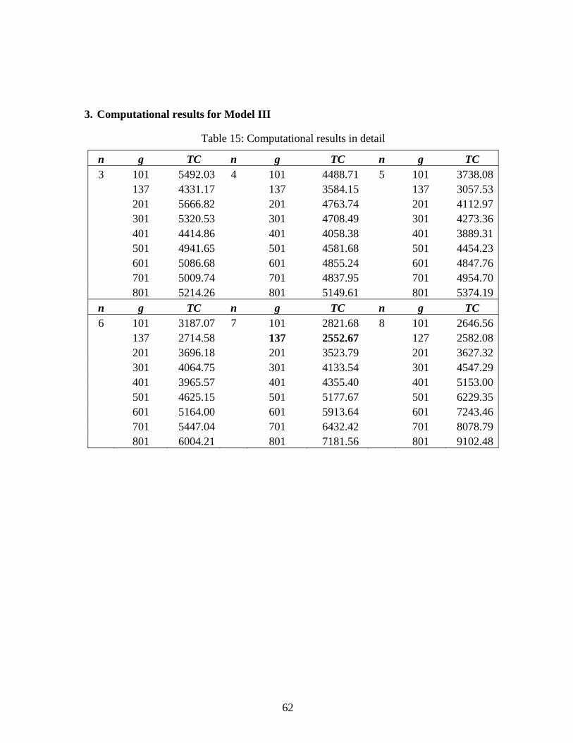
62

3. Computational results for Model III


n g TC n g TC n g TC 3 101 5492.03 4 101 4488.71 5 101 3738.08 137 4331.17 137 3584.15 137 3057.53 201 5666.82 201 4763.74 201 4112.97 301 5320.53 301 4708.49 301 4273.36 401 4414.86 401 4058.38 401 3889.31 501 4941.65 501 4581.68 501 4454.23 601 5086.68 601 4855.24 601 4847.76 701 5009.74 701 4837.95 701 4954.70 801 5214.26 801 5149.61 801 5374.19

n g TC n g TC n g TC 6 101 3187.07 7 101 2821.68 8 101 2646.56 137 2714.58 137 2552.67 127 2582.08 201 3696.18 201 3523.79 201 3627.32 301 4064.75 301 4133.54 301 4547.29 401 3965.57 401 4355.40 401 5153.00 501 4625.15 501 5177.67 501 6229.35 601 5164.00 601 5913.64 601 7243.46 701 5447.04 701 6432.42 701 8078.79 801 6004.21 801 7181.56 801 9102.48

63

VITA

Chiranjit Saha was born to Mr. Ranjit Saha (father) and Mrs. Sipra Saha (mother) in

Kolkata, India, in 1984. He earned a Bachelor of Science in Electronics and Instrumentation

Engineering from West Bengal University of Technology, Siliguri, India in 2006. He joined

the Department of Construction Management and Industrial Engineering at Louisiana State

University at Baton Rouge, Louisiana, in fall 2007 for the degree of Master of Science in

Industrial Engineering.

an operational policy for a single vendor multi buyer

Documents