Measurement 92 (2016) 340–351

Contents lists available at ScienceDirect

Measurement

journal homepage: www.elsevier .com/locate /measurement

An online two-stage adaptive algorithm for strain profile estimationfrom noisy and abruptly changing BOTDR data and application tounderground mines

http://dx.doi.org/10.1016/j.measurement.2016.06.0220263-2241/� 2016 Elsevier Ltd. All rights reserved.

⇑ Corresponding author.E-mail address: gsoto@dim.uchile.cl (G. Soto).

G. Soto a,⇑, J. Fontbona a, R. Cortez a, L. Mujica b

aCenter for Mathematical Modeling (CMM), UMI (2807), UCHILE-CNRS, ChilebMining Information Communications and Monitoring (Micomo), Fundación Chile, Chile

a r t i c l e i n f o a b s t r a c t

Article history:Received 3 June 2015Received in revised form 13 May 2016Accepted 13 June 2016Available online 16 June 2016

Keywords:BOTDRBrillouin gain spectrumStrainTime seriesSmoothingOutliersAbrupt changes

Strain measurement using BOTDR (Brillouin Optical Time-Domain Reflectometry) is nowadays a standardtool for structural health monitoring. In this context, weak data quality and noise, usually owed to defec-tive fiber installation, hinders discriminating actual level shifts from outliers and might entail a biasedrisk assessment. We propose a novel online adaptive algorithm for strain profile estimation in strain timeseries with abrupt and gradual changes and missing data. It relies on a convolution filter in Brillouin spec-trum domain and a smoothing technique in time domain. In simulated data, the convolution filter isshown to reduce strain measurement uncertainty by up to 8 times the strain resolution. The two-stagemethod is illustrated with systematic outliers removal from real data of a Chilean copper mine andthe improvement of the associated gain spectrum quality by up to 18 dB in SNR terms.

� 2016 Elsevier Ltd. All rights reserved.

1. Introduction

Distributed fiber sensors technology based on Brillouin scatter-ing has attracted much attention for remarkable features such asits high precision, high spatial resolution and long measuring range[1]. Structural deformation monitoring based on Brillouin OpticalTime-Domain Reflectometry (BOTDR) allows the measurement ofthe longitudinal strain applied along an optical fiber attached toa structure, by means of the Brillouin gain spectrum [2]. If thestructure suffers a deformation, a change in the shape of the spec-trum measured by the BOTDR system is observed. The behavior ofthe structure subjected to strength can then be assessed by meansof suitable physical and statistical models. Among other uses, thistechnique has been applied to civil structural monitoring [3,4],roadworks [5,6], and mining [7–9].

It is well known that, when an optical pulse is launched into anoptical fiber, some backscattered signals come back to the inputend. The BOTDR system measures the power distribution infrequency of the backscattered light at each point along to the opti-cal fiber. This distribution, called Brillouin gain spectrum (BGS),can be seen as a set of Lorentzian-like curves along the distance

coordinate. When a longitudinal strain � is applied to the fiber,and as a result of the non-linear interaction between the incidentlight and acoustic phonons of the crystal lattice of the semiconduc-tor material, the backscattered light is shifted in frequency by anamount mB, called Brillouin shift [10,11]. This applied longitudinalstrain � is related to the value of the frequency shift [12,13]through the linear relationship mBð�Þ ¼ mBð0Þð1þ C�Þ, where mBð�Þstands for the Brillouin frequency shift after strain has beenapplied, mBð0Þ is a referential Brillouin frequency shift and C isthe proportional coefficient of strain [14].

The frequency shift is standardly estimated by fitting a Lorent-zian function to the spectrum at each point of the optical fiber anddetermining its mode or central value. This fitting procedure isusually done by means of suitable least squares minimizationalgorithms [15]. This method presents an important drawback:the accuracy of the estimation of the strain-BOTDR can be consid-erably affected by measurement noise, which can bias the estima-tion of mB and result in multiple outliers in the strain time series.The presence of outliers could prevent from correctly discriminat-ing whether a true level shift has occurred or not, and mislead theinstantaneous analysis of time series. Consequences of this could insome cases be serious, especially if the sampling rate of the onlinestrain-BOTDR monitoring is low, since the confirmation or rectifi-cation of the measured level shift by means of new measurements

Fig. 1. An observed Brillouin gain spectrum frame, taken from of a sequence of realdata registered at El Teniente (Codelco) mine in Chile during 2008. The datadescription and the BOTDR system setting is detailed in Section 5.3.

G. Soto et al. /Measurement 92 (2016) 340–351 341

could arrive too late. Therefore, there is strong a necessity for arobust procedure that estimates strain profile consistently overtime and along the fiber.

To address this problem, this paper proposes an adaptive algo-rithm for strain profile estimation from low-quality BOTDR data, inthe context of an online procedure. Our methodology is suitable forforecasting the statistical behavior of Brillouin gain spectra withboth abrupt and gradual changes over time, and is robust againstoutliers.

Spectral noise can be seen as a stochastic process followingsome trivariate underlying joint distribution that depends on twoexplanatory variables of the BGS, namely the distance x and thefrequency m, and on a time variable t inherent to the time series.We are therefore faced a 3-dimensional estimation problem, whichwe will address by means of the simultaneous use of two tech-niques. The first technique consists in a convolution filter on theðx; mÞ domain whose main feature is the ability to keep the valueof mB unchanged at the observed spectral distribution. The secondone is an exponential smoothing technique for temporal noisereduction, using a time series model consisting of a linear trendwith an additive noise term. In addition, our temporal estimationtechnique is robust enough to deal with missing data and abruptchanges in the level, a situation often found in practice whichaffects the performance of standard filtering techniques.

Although some of the aforementioned papers deal with somestatistical aspects of Brioullin shift estimation, to our knowledgethe only available method which also addresses the problem ofglobal consistent space–time estimation, is the procedure basedon 3d Non Local Means (NLM) presented in the paper [16] (whichappeared while the present work was in its revision stage). Com-parative discussions will be given later at several places, in partic-ular when we will asses the performance and computational costof our method.

The remainder of this paper is organized as follows. In Section 2we discuss the effect of noise on the BGS and the methodology pro-posed to reduce it. We describe the observation data model in Sec-tion 3. In Section 4 we propose a pseudo two-dimensionalconvolution filter to estimate the underlying (unnoisy) spectraldistribution in the distance-frequency domain. Its performance isassessed in Section 5 both theoretically and by means of Monte-Carlo simulations. The temporal filtering method based on expo-nential smoothing is described in Section 6. Section 7 presentsthe algorithm combining the two previous stages. The algorithmis applied on real data from El Teniente mine (Codelco, Chile) inSection 8 and the obtained results are then discussed. The compu-tational cost of our method in a general sensing framework is dis-cussed in Section 9. Finally, Section 10 brings the conclusions of thepaper.

2. The problem of measurement-noise in Brillouin gainspectrum

The intrinsic variations of the strain time series, in combinationwith suitable forecasting models, are commonly used for structuralhealth monitoring or assessment of structural instabilities. How-ever, the accuracy of these analysis heavily depend on the qualityof the measured Brillouin gain spectrum (BGS) which often con-tains noise. The BOTDR system records a sequence of spectra witha given sampling rate s, measured in hours. The observed BGS canbe seen as a frame of this sequence. A typical noisy BGS obtainedby the BOTDR system is shown in Fig. 1, which corresponds to aframe of a sequence of real data taken from a Chilean undergroundcopper mine (a detailed description of this data and the BOTDRsystem setting used to obtain it will be given in Section 5.3).

As mentioned in the introduction, if the spectral noise varianceis large enough, outliers owed to a biased Brillouin frequency shiftestimation can appear in the strain time series, which couldprevent the correct detection of true level shifts and entail a biasedrisk assessment, with potentially serious consequences. This moti-vates the development of statistical tools that simultaneouslyreduce the effects of the spectral noise and provide coherent obser-vation sequences in presence of temporally varying fieldconditions.

The approach we propose to reduce the spectral noise is basedon separating the problem in two stages, developed in the follow-ing sections: (1) applying a filtering technique in the distance-frequency coordinate and (2) applying then a temporal filteringtechnique. Firstly, the underlying BGS is estimated by applying apseudo 2-dimensional convolution filter designed in thedistance-frequency domain, and then, a temporal smoothing tech-nique is carried out using a locally linear regression model, whichmaintains over time the coherence of the distance-frequency coor-dinates of the filtered data.

3. Observation model

We next introduce a simple model for the evolution of theobserved variations of the BGS. Let S and T be two sets such thatS � R2 and T � R. We consider the observed BGS as a noisy2-dimensional sequence M : S � T ! R defined as

Mðs; tÞ ¼ Bðs; tÞ þ �ðs; tÞ; s 2 S; t 2 T ; ð1Þ

where Bðs; tÞ is the original BGS, ðs; tÞ represents the coordinate inthe S � T domain, with s ¼ ðx; mÞ, and eðs; tÞ � f e is an additive noisethat follows some trivariate distribution.

Notice we have not yet given a regression model for the tempo-ral behavior of the rock mass itself, which is represented by thesequence Bðs; tÞ and can be specified independently. Such a modelwill be presented below.

According to the model, the aim of the proposed filtering

method is to provide an estimate eB of the original BGS, B, fromthe observed data, M, separating the task into two fundamentalstages: a 2-dimensional filtering technique in the S-domain anda smoothing technique for time series in the T -domain.

Fig. 2. A filtered Brillouin gain spectrum, resulting from applying the convolutionfilter with Ch ¼ 20 MHz on the spectrum of Fig. 1.

342 G. Soto et al. /Measurement 92 (2016) 340–351

4. Filtering in the S-domain

4.1. The problem statement

The problem of the spectral estimation at a fixed time t, can bestated as follows. Let s ¼ ðx; mÞ be the distance-frequency coordi-nate. The observation model defined in (1) can be rewritten as

mðx; mÞ ¼ bðx; mÞ þ �ðx; mÞ; x 2 X ; m 2 V; ð2Þ

with S ¼ X � V � R2, where mðx; mÞ is a frame of the sequenceMðs; tÞ corresponding to the observed BGS measured by the BOTDRsystem at a fixed time t, and the additive noise � � f � follows somebivariate distribution.

In addition to outliers removal, when estimating the originalspectrum b from a noisy observation m by applying a2-dimensional convolution filter, the method we propose will keepunchanged two fundamental features of the data, namely (a) thecentral frequency md of the Lorentzian distribution at each point xalong to the optical fiber, and (b) the spatial resolution of theBOTDR system.

4.2. The convolution filter

It is known that the implementation of a classical low-pass fil-tering technique is highly affected by the tradeoff between noisereduction and bias. The choice of a suitable value for the smoothingparameter plays a rather crucial role. A too large value can exces-sively blur some areas of high curvature, which results in a largebias. This means that, if we applied a filter with this feature onthe distance domain of a noisy BGS, we then reduce the spatial res-olution of the BOTDR system, and consequently, the estimate ofstrain profile will be biased.

In order to prevent a large bias in the distance-frequencydomain, the proposed filter hðx; m;ChÞ consists in a Lorentzian func-tion, centered at 0, defined as

hðx; m;ChÞ ¼gh

pCh

m2 þ C2h

ð3Þ

where gh is the gain of the filter and Ch is a smoothing parameterthat controls the filtering quality. This parameter is also called FullWidth at Half Maximum (FWHM). The filter (3) is applied in eachposition x along the fiber, as a 1-dimensional convolution betweenthe (noisy) observed Brillouin distribution and this filter. In otherwords, we only take into account the frequency domain for denois-ing this 2-dimensional data, and this is the reason why the pro-posed filter is referred as a ‘‘pseudo 2-dimensional technique”. Inthis manner, our approach allows for reducing the spectral noisewithout affecting the spatial resolution of the system, since thefilter does not smooth areas of high curvature in the distancedomain of the BGS.

On the other hand, since the accuracy of the central frequencyestimation by Lorentzian fitting depends on how noisy anddeformed the spectral distribution is, we have chosen this filterbecause of a fundamental fact: the convolution between two Lor-entzian curves results in a curve with Lorentzian distribution.

Indeed, suppose that the (unknown) original spectrum bðx; mÞ inmodel (2) can be represented by a family of Lorentzian distribu-tions with local central frequency mbðxÞ, as follows:

bðx; mÞ ¼ gbðxÞp

CbðxÞðm� mbðxÞÞ2 þ C2

bðxÞð4Þ

where CbðxÞ and gbðxÞ stand for the FWHM and the maximum valueof the original spectrum at the distance x along the fiber. We define~bðx; mÞ, the estimate of the original BGS bðx; mÞ at instant t, in the fol-lowing way

~bðx; mÞ ¼ mðx; mÞ � hðx; m;ChÞ; ð5Þ

where � is the convolution operator. Then, applying (3) in (2)according to relationships (5) and (4), we obtain that

~bðx; mÞ ¼ bðx; m; hxÞ þ gðx; mÞ ð6Þ

bðx; m; hxÞ ¼gbðxÞp

CbðxÞðm� mbðxÞÞ2 þ C2

bðxÞ; ð7Þ

gðx; mÞ ¼ hðx; m;ChÞ � �ðx; mÞ ð8Þ

with

hx ¼ ½mbðxÞ;CbðxÞ; gbðxÞ� ð9ÞmbðxÞ ¼ mbðxÞ ð10ÞgbðxÞ ¼ ghgbðxÞ ð11ÞCbðxÞ ¼ CbðxÞ þ Ch; ð12Þ

where hx; mbðxÞ;CbðxÞ, and gbðxÞ stand for the estimated parametervector, the central frequency, the FWHM and the maximum value

of the filtered spectrum ~bðx; mÞ at the distance x, respectively. From(6) and (7), the estimated spectrum is again given by a Lorentziandistribution plus some noise. Therefore, the characteristic shape ofthe estimated spectrum does not suffer from meaningful changes.Most importantly, we have mbðxÞ ¼ mbðxÞ, that is, the central fre-quency value of the Lorentzian curve is kept unchanged and, conse-quently, the strain associated with the Brillouin frequency shift too.In Fig. 2, we show the result of applying the filter hðx; m;ChÞ withCh ¼ 20 MHz to the spectrum of Fig. 1.

Furthermore, the noise level has been reduced by the convolu-tion hðx; m;ChÞ � �ðx; mÞ, where the filtering performance is beingcontrolled by the parameter Ch. We also observe an increase ofthe FWHM CbðxÞ when compared to the value CbðxÞ of the mea-sured BGS, but this result does not affect, theoretically at least,the estimation of the frequency shift. In Ref. [17], by using differentpump pulse widths, experimental results about the impact of theFWHM on the frequency error are shown. Errors do not exceed1 MHz (10�3 GHz), a relatively small value compared to typical val-ues of the frequency shifts, which are the order of 10 GHz.

G. Soto et al. /Measurement 92 (2016) 340–351 343

5. The filtering performance

5.1. Signal-to-noise ratio

Signal-to-noise ratio (SNR) is a good measure of the filteringperformance, since it describes how much a signal has been cor-rupted by noise. Let PS and PN be the discrete average power ofthe Brillouin gain spectrum and the spectral noise, respectively.Then, in decibels (dB), the SNR is defined as

SNR ¼ 10log10PS

PN

� �: ð13Þ

Note that, if the noise is zero mean, the power of noise isdefined by only its variance. In this manner, the SNR can written as

SNR ¼ 10log10PS

r2

� �; ð14Þ

where r2 stands for the noise variance.This definition will be used later in the assessment of frequency

shift estimators respect to sensitivity to noise, and consequently,respect to the impact of noise effects ondeformationmeasurements.

5.2. Estimator performance using synthetic data

It is important to determine quantitatively the magnitude of thefilter effect, in order to be able to reduce the possible effects of thespectral noise, such as outliers. The Cramér-Rao theorem (see [18]for background) provides a strict lower bound for the variance of aquantity which is estimated from a set of noisy measurements,and can be applied to determine the (theoretical) minimum uncer-tainty in the determination of the Brillouin Frequency Shift ordeformation.

5.2.1. Cramér-Rao lower boundLet us assume that a noisy spectrum with central frequency h

was generated by adding to it a Gaussian zero mean noise of vari-ance r2. Thus, the Brillouin spectrum can be written as

mi ¼ biðhÞ þ r�i; i ¼ 1; . . . ; n ð15Þ

with �i � Nð0;1Þ, where

biðhÞ ¼gb

pCb

ðmi � hÞ2 þ C2b

; ð16Þ

is the unnoisy Brillouin spectrum, that is, the spectrum withouteffects induced by the BOTDR system. Then, if we assume thatr; gb and Cb are known, it can be shown that the variance of anyunbiased maximum likelihood estimator h is

varðhÞP r2CR ð17Þ

where r2CR is called the Cramér-Rao Lower Bound (CRLB) (see [18]),

with

rCR ¼rffiffiffiffiffiffiffiffiffiffiffiffiffiffiffiffiffiffiffiffiffiffiffiffiffiffiffiPn

i¼1dbiðhÞdh

� �2r : ð18Þ

It is worth noting that if biðhÞ is the identity function (biðhÞ ¼ h), wehave that varðhÞP r2=n, as might be expected. Now, computing thederivate of biðhÞ respect to h, we finally have

rCR ¼p

2gbCb

ffiffiffiffiffiffiffiffiffiffiffiffiffiffiffiffiffiffiffiffiffiffiffiffiffiffiffiffiffiffiffiffiffiffiffiffiffiPni¼1

mi�hðmi�hÞ2þC2

b

� �2s r: ð19Þ

This theoretical bound will be used as a benchmark for assessingthe impact of the noise on deformation measurements.

5.2.2. Monte Carlo simulationA simulation study was conducted to compare the performance

of the Lorentzian curve fitting respect to the sensitivity to noise,when previously using, or not, a convolution filter for denoising.The performance is assessed by comparing the Root Mean SquaredError (RMSE) of the estimate h, whose value corresponds to thestandard deviation of an unbiased estimator, with the CRLB, thatis, the theoretical bound for the standard deviation given byEq. (19). RMSE is computed as the expected value of the meansquared difference between the estimated values h and the under-lying true value mo, using synthetic data fmi : i ¼ 1; . . . ;ng as follows

RMSEðhÞ ¼ ðE½ðmo � hÞ2�Þ1=2

: ð20Þ

The expected value E is approximated by the Monte Carloestimate

E½ðmo � hÞ2� ¼ 1R

XRr¼1ðmo � hrÞ

2; ð21Þ

where hr stands for the rth estimate of true value h ¼ mo.Let giðhÞ be the fitting error, defined as follows

giðhÞ ¼ mi � hiðChÞ � biðhÞ; ð22Þ

where mi stands for the noisy spectrum, hi stands for the convolu-tion filter defined as

hiðChÞ ¼gh

pCh

ðmi � hÞ2 þ C2h

: ð23Þ

and biðhÞ is the spectrum model defined as

biðhÞ ¼ghgb

pCb þ Ch

ðmi � hÞ2 þ ðCb þ ChÞ2: ð24Þ

Since we assume that the noise is governed by a Normal distri-bution, the maximum likelihood estimation of h can be estimatedby non-linear least squares as follows

h ¼ arg minh2H

Xni¼1

g2i ðhÞ: ð25Þ

Simulation were repeated R ¼ 1000 times to make results inde-pendent of any particular observation. Noisy spectra are generatedusing the model given by Eq. (15) using different values of noisevariance r2. From Eq. (14), and knowing that the power of biðmoÞ is

PS ¼1n

Xni¼1

b2i ðmoÞ; ð26Þ

the noise variance is computed as

r2 ¼ PS10�SNR

10 : ð27Þ

Fixed parameters were set to gb ¼ gh ¼ 1 by simplicity, andCb ¼ 25 MHz, according to the BOTDR system setting. The scaninterval of simulated spectra was set to 10 MHz in a range of fre-quencies from 10.62 to 11.11 GHz. In Fig. 3 the result of computingthe CRLB on this range of frequencies is shown. Aside fromsequences close to the upper or lower bounds of the range, the resthas the same value of CRLB. Therefore, we take a value from thatrange for simulations. In this manner, we choose mo ¼ 10:85 GHzas the value of the (true) Brillouin frequency shift to estimate,because this value belongs to the range of minimum CRLB and italso corresponds to the case when the fiber does not have deforma-tion, according to the BOTDR system setting.

Fig. 4 shows results of the simulation in which the accuracy ofthe unfiltered and pre-filtered estimator are only comparable forSNR values greater than 2 dB, practically all estimators attainingthe CRLB after 5 dB. Although the performance of pre-filtered

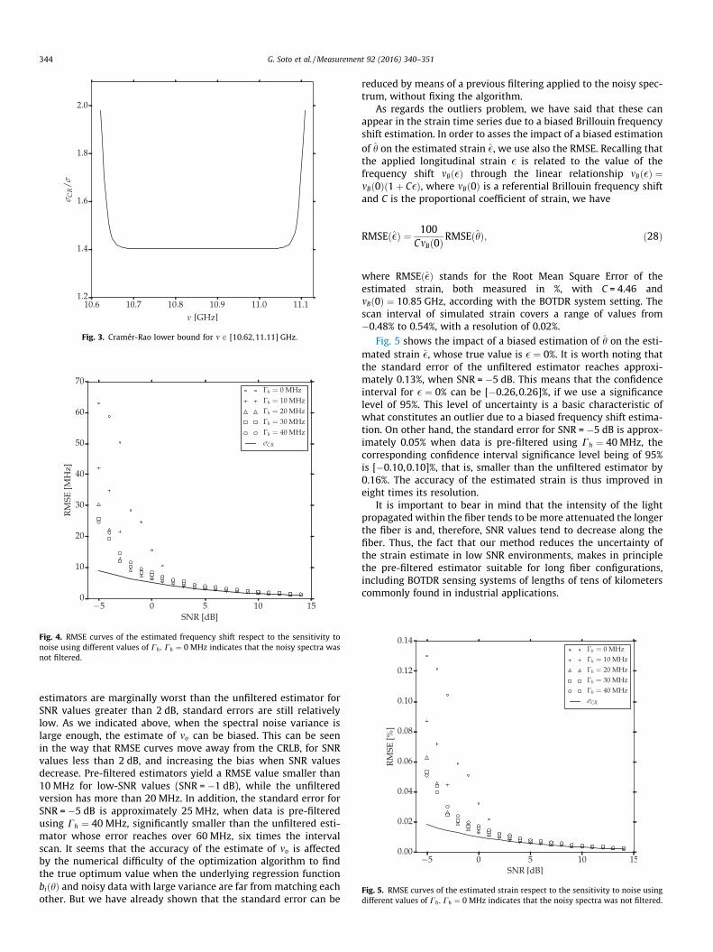
Fig. 3. Cramér-Rao lower bound for m 2 [10.62,11.11] GHz.

Fig. 4. RMSE curves of the estimated frequency shift respect to the sensitivity tonoise using different values of Ch . Ch ¼ 0 MHz indicates that the noisy spectra wasnot filtered.

Fig. 5. RMSE curves of the estimated strain respect to the sensitivity to noise usingdifferent values of Ch . Ch ¼ 0 MHz indicates that the noisy spectra was not filtered.

344 G. Soto et al. /Measurement 92 (2016) 340–351

estimators are marginally worst than the unfiltered estimator forSNR values greater than 2 dB, standard errors are still relativelylow. As we indicated above, when the spectral noise variance islarge enough, the estimate of mo can be biased. This can be seenin the way that RMSE curves move away from the CRLB, for SNRvalues less than 2 dB, and increasing the bias when SNR valuesdecrease. Pre-filtered estimators yield a RMSE value smaller than10 MHz for low-SNR values (SNR = �1 dB), while the unfilteredversion has more than 20 MHz. In addition, the standard error forSNR = �5 dB is approximately 25 MHz, when data is pre-filteredusing Ch ¼ 40 MHz, significantly smaller than the unfiltered esti-mator whose error reaches over 60 MHz, six times the intervalscan. It seems that the accuracy of the estimate of mo is affectedby the numerical difficulty of the optimization algorithm to findthe true optimum value when the underlying regression functionbiðhÞ and noisy data with large variance are far from matching eachother. But we have already shown that the standard error can be

reduced by means of a previous filtering applied to the noisy spec-trum, without fixing the algorithm.

As regards the outliers problem, we have said that these canappear in the strain time series due to a biased Brillouin frequencyshift estimation. In order to asses the impact of a biased estimationof h on the estimated strain �, we use also the RMSE. Recalling thatthe applied longitudinal strain � is related to the value of thefrequency shift mBð�Þ through the linear relationship mBð�Þ ¼mBð0Þð1þ C�Þ, where mBð0Þ is a referential Brillouin frequency shiftand C is the proportional coefficient of strain, we have

RMSEð�Þ ¼ 100CmBð0Þ

RMSEðhÞ; ð28Þ

where RMSEð�Þ stands for the Root Mean Square Error of theestimated strain, both measured in %, with C = 4.46 andmBð0Þ ¼ 10:85 GHz, according with the BOTDR system setting. Thescan interval of simulated strain covers a range of values from�0.48% to 0.54%, with a resolution of 0.02%.

Fig. 5 shows the impact of a biased estimation of h on the esti-mated strain �, whose true value is � ¼ 0%. It is worth noting thatthe standard error of the unfiltered estimator reaches approxi-mately 0.13%, when SNR = �5 dB. This means that the confidenceinterval for � ¼ 0% can be [�0.26,0.26]%, if we use a significancelevel of 95%. This level of uncertainty is a basic characteristic ofwhat constitutes an outlier due to a biased frequency shift estima-tion. On other hand, the standard error for SNR = �5 dB is approx-imately 0.05% when data is pre-filtered using Ch ¼ 40 MHz, thecorresponding confidence interval significance level being of 95%is [�0.10,0.10]%, that is, smaller than the unfiltered estimator by0.16%. The accuracy of the estimated strain is thus improved ineight times its resolution.

It is important to bear in mind that the intensity of the lightpropagated within the fiber tends to be more attenuated the longerthe fiber is and, therefore, SNR values tend to decrease along thefiber. Thus, the fact that our method reduces the uncertainty ofthe strain estimate in low SNR environments, makes in principlethe pre-filtered estimator suitable for long fiber configurations,including BOTDR sensing systems of lengths of tens of kilometerscommonly found in industrial applications.

Fig. 6. Variation of the SNR using a filtered BGS sequence with different values ofCh . The curve Ch ¼ 0 MHz stands for the variation of the SNR using the unfilteredsequence.

G. Soto et al. /Measurement 92 (2016) 340–351 345

5.3. Filtering performance using real data

We next assess the estimator when the convolution filter isapplied to a real time BGS sequence, obtained in a fiber sectioninstalled inside El Teniente mine of Chilean state mining companyCodelco.

These measurements were carried out with a sampling rate ofs ¼ 4 h. In total there are 165 frames, which cover 728 h(� 30 days) of regular samples, with some missing data. The fiberunder analysis is 4.94 m long, and a sampling rate of 10 cm wasused, making a total of 494 samples. The frequency resolution ofthe BOTDR system was set to 10 MHz in a range of frequenciesfrom 10.62 to 11.11 GHz, which means we have 50 samples.Through the linear relationship between strain and frequency shift,the BOTDR system is able to measure deformation in intervals of0.02%, from�0.48% to 0.54%, with a spatial resolution of 1 m, underthis setting.

Unlike the previous assessment, SNR will be used as an indica-tor of improved data quality as well as of the stability of thisimprovement over time.

Let PS and PN be the discrete average power of the Brillouin gainspectrum and the spectral noise, respectively. These are computedas follows:

PS ¼1jXjjVj

Xx2X

Xm2Vfbðx; mÞg2; ð29Þ

PN ¼1jXjjVj

Xx2X

Xm2Vfgðx; mÞg2: ð30Þ

Since values of PS and PN are unknown, we will estimate them viaLorentzian-curve fitting using non-linear least squares.

Let gðx; m; hxÞ be the fitting error, whose expression is defined asfollows

gðx; m; hxÞ ¼ ~bðx; mÞ � bðx; m; hxÞ; ð31Þ

where ~bðx; mÞ stands for the measured spectrum, bðx; m; hxÞ is thespectrummodel defined in (7) and hx is the parameter model at dis-tance x. If we assume that the noise is governed by a Normal distri-bution, the maximum likelihood estimation of hx can be estimatedby non-linear least squares as follows

hLFx ¼ arg minhx2H

Xm2Vfgðx; m; hxÞg2; ð32Þ

where hLFx is the estimate of hx by means of Lorentzian-curve fittingin the frequency domain. Taking into account definitions (29) and(30), and the fact that the spectrum and the noise can be estimatedby

bðx; mÞ ’ bðx; m; hLFx Þ ð33Þgðx; mÞ ’ gðx; m; hLFx Þ ð34Þ

we can now estimate the SNR in Eq. (13), using the expression

SNR ’ 10log10

Xx2X

Xm2Vfbðx; m; hLFx Þg

2

Xx2X

Xm2Vfgðx; m; hLFx Þg

2

0BB@1CCA: ð35Þ

Fig. 6 shows the filtering performance of the proposed filter fordifferent values of Ch, where SNR values are estimated using thesequence of real data from El Teniente mine. It should also benoted that the SNR value varies over time in the sequence, reachingthe lowest level at t = 608. These variations might have severalcauses like, for instance, a faulty installation of the optical fiberattached to the monitored structure. The curves show that the pro-posed filter achieves an improvement at the data quality (highSNR) as the value of Ch increases, as well as a reduction of temporal

variations of the noise variance, due to a slower SNR decay withrespect to unfiltered sequence, especially when using Ch P20 MHz.

The proposed temporal smoothing technique, for maintainingthe spatial coherence of the filtered data over time, is detailed next.

6. Filtering in the T -domain

Recursive methods in time series consist in adaptation of a pre-vious estimate by means of a correction term which depends bothon the previous estimate and on a new observation. Due to theirsimplicity and good performance, they are successfully used forestimation, smoothing and forecasting in time series analysis. Inthis section, we describe our proposed method for temporalsmoothing, based on a particular robust version of the Holt–Win-ters method. This version is able to estimate the model parametersin presence of abrupt and gradual trends and when observationsare missing.

6.1. The Holt–Winters method

Suppose we have an univariate time series yn, which is observedat n ¼ 1; . . . ;N. The observation model is given by

yn ¼ ln þ nn; nn � f n; ð36Þ

where ln stands for the original (unnoisy) observation at time n,and nn is an additive noise that follows a one-dimensional distribu-tion f n. In the case of exponentially weighted moving average(locally constant regression), the value of the smoothed series attime n, ~ln, is the solution of the following minimization problem[19]:

~ln ¼ arg minln2H

Xnk¼1ð1� aÞn�kfyk � lng

2 ð37Þ

where a is a parameter taking values between 0 and 1 which con-trols the degree of smoothing.

It is possible to show that the solution of the optimization prob-lem (37) can be solved by means of the following recursiveequation

346 G. Soto et al. /Measurement 92 (2016) 340–351

~ln ¼ ayn þ ð1� aÞlnjn�1; ð38Þ

where lnjn�1, the one-step-ahead forecast of yn based on previous

observations fykgn�1k¼1 , is obtained as

lnjn�1 ¼ ~ln�1: ð39Þ

The recursive Eq. (38) suggests that, if the underlying mean is sub-ject to large changes, a should be taken close to 1 so as to quicklyattenuate the effect of old observations. However, if a is too closeto 1, ~ln is subject to much higher random variations, because ofan under-smooth estimated mean. The rate at which informationis discounted is characterized by the asymptotic sample length(ASL), defined by

ASL ¼ 1a; ð40Þ

and corresponds to the number of samples per length unit of thedata window within which the contribution of the error values issignificant. Clearly, when a ¼ 0, the length of the data windowbecomes infinite and we obtain the standard least squares method.If we use values of a between 0.01 and 0.1, values of ASL lie in therange of 10–100 time samples, which corresponds to 40–400 h ofdata, according to the BOTDR system setting.

In order to improve theperformanceof themethod in presence oftrended time series,Holt [20] andWinters [21]proposed to includealocal linear trendvariable,with regressionmodel of the general formut þ v tt, by solving the following minimization problem:

ð~un; ~vnÞ ¼ arg minun ;vn2H

Xnk¼1ð1� aÞn�kfyk � ðun þ vnksÞg2: ð41Þ

The recursive equations to solve (41) are

~un ¼ ayn þ ð1� aÞunjn�1 ð42Þ

~vn ¼ b~un � ~un�1

sþ ð1� bÞ~vnjn�1 ð43Þ

where ~un y ~vn are the level and trend, respectively, s is the samplingrate and a ¼ b in general, according to (41); nevertheless, differentvalues for smoothing the two parameters are commonly used inpractice. In a similar way as for exponential smoothing, the smooth-ing parameters a and b take values between zero and one. Then,unjn�1 and vnjn�1, the one-step-ahead forecast of yn and of _yn, respec-tively, are obtained as

unjn�1 ¼ ~un�1 þ s~vn�1 ð44Þvnjn�1 ¼ ~vn�1: ð45Þ

where ~un�1 and ~vn�1 are the level and trend estimated at time n�1,respectively.

Extending this method to the multidimensional case, whereMðs; nÞ denotes the BGS measured by the BOTDR system at timen, Eqs. (42) and (43) represent an adaptive filtering technique toestimate Bðs;nÞ, the original (unnoisy) BGS, when changes in thelevel of the observed sequence are gradual. Then, the observationmodel (1) can be rewritten as

Mn ¼ Bn þ en; en � f e ð46Þ

where Mn � Mðs;nÞ;Bn � Bðs;nÞ, and en � eðs;nÞ.Rewriting (42) and (43), the estimation of Bn at time n is carried

out using the following update equations:eBn ¼ aMn þ ð1� aÞbBnjn�1 ð47Þ

eDn ¼ beBn � eBn�1

sþ ð1� bÞbDnjn�1 ð48Þ

where eBn denotes the estimation of Bn and eDn its temporal varia-tion. Finally, the one-step-ahead forecast value of Bn based on

previous observations fBkgn�1k¼1 ;bBnjn�1, and the forecast of its tempo-

ral variation, bDnjn�1, are given by

bBnjn�1 ¼ eBn�1 þ seDn�1 ð49ÞbDnjn�1 ¼ eDn�1: ð50Þ

6.2. Extended method for missing data

Sometimes, BOTDR data are missed, for instance because of anaccidental break of the optical fiber produced by mining activitiesin the nearby area. If the smoothing parameters are taken to beconstant over time, this may result in estimation errors, due toinadequate weights on older observations in the update equations.

To solve this problem, we use the extended Holt–Wintersmethod introduce in [22] to deal with time series observed atirregular time intervals. If we assume that Mtn is the observedBGS measured by the BOTDR system at time tn, Eq. (46) can berewritten as

Mtn ¼ Btn þ etn ; etn � f e ð51Þ

where Btn is the original (unnoisy) BGS and etn is a zero-mean addi-tive noise at time tn. Then, the forecasting model is defined as

bBtn jtn�1 ¼ eBtn�1 þ ðtn � tn�1ÞeDtn�1 ð52ÞbDtn jtn�1 ¼ eDtn�1 ; ð53Þ

where bBtn jtn�1 stand for the one-step-ahead forecast value of Btn

based on the estimates of BGS at time tn�1, and bDtn jtn�1 is the forecastof its temporal variation. Note that the factor tn � tn�1 weights tem-poral variations according to the time-distance between two con-secutive measurements.

To update the parameters of model (51), we need to modify therecursive Eqs. (47) and (48) so that smoothing parameters can alsobe updated as needed. In this manner, update equations are rewrit-ten as follows

eBtn ¼ atnMtn þ ð1� atnÞbBtn jtn�1 ð54Þ

eDtn ¼ btn

eBtn � eBtn�1

tn � tn�1þ ð1� btnÞbDtn jtn�1 ; ð55Þ

where eBt0 ¼ Mt0 and eDt0 ¼ 0 are initial conditions.Taking into account the time span tn � tn�1 between two con-

secutive observations, and the sampling rate s, we update thesmoothing parameters as follows

atn ¼atn�1

ð1� aÞtn�tn�1

s þ atn�1

ð56Þ

btn ¼btn�1

ð1� bÞtn�tn�1

s þ btn�1

: ð57Þ

Initial conditions are fixed at at0 ¼ a and bt0 ¼ b. Clearly, ifobservations are regularly sampled, with tn � tn�1 ¼ s, thenatn ¼ a and btn ¼ b;8tn.

Parameters a and b are commonly know as forgetting factors.Values of a and b are chosen looking for trade-off between conver-gence velocity of the algorithm and variance of the estimation.

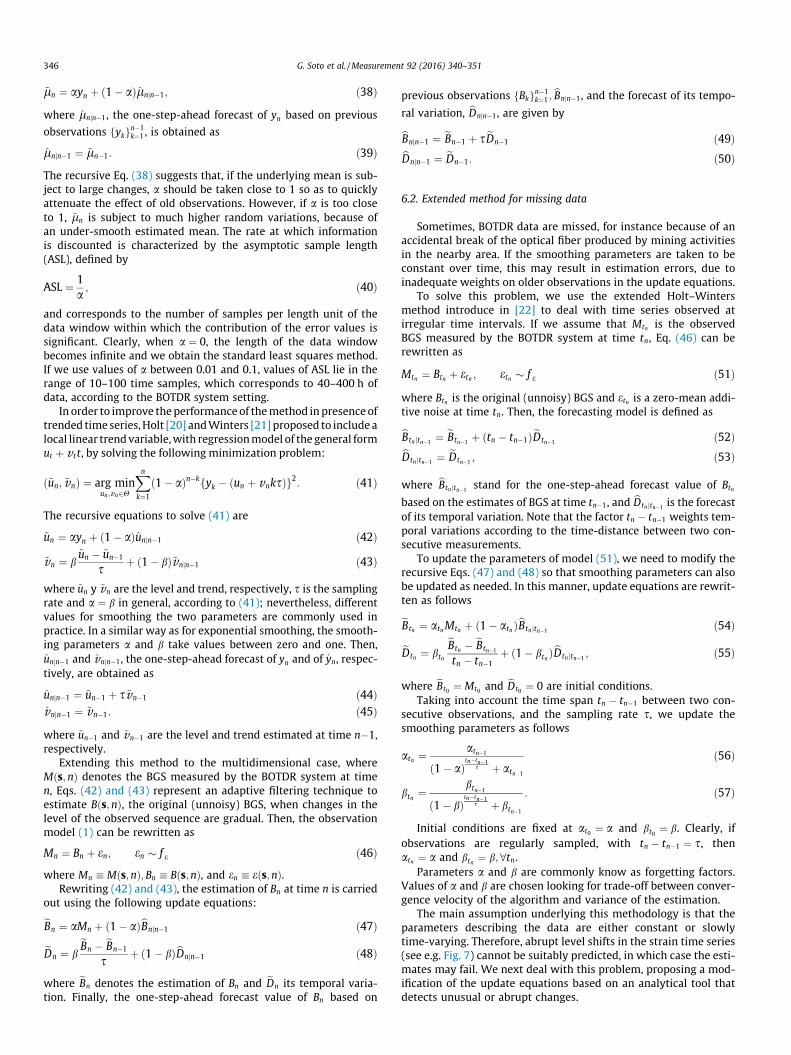
The main assumption underlying this methodology is that theparameters describing the data are either constant or slowlytime-varying. Therefore, abrupt level shifts in the strain time series(see e.g. Fig. 7) cannot be suitably predicted, in which case the esti-mates may fail. We next deal with this problem, proposing a mod-ification of the update equations based on an analytical tool thatdetects unusual or abrupt changes.

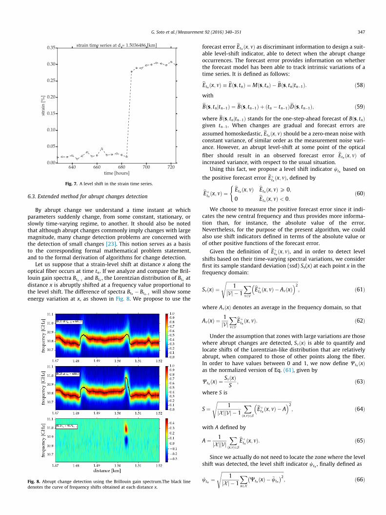
Fig. 7. A level shift in the strain time series.

G. Soto et al. /Measurement 92 (2016) 340–351 347

6.3. Extended method for abrupt changes detection

By abrupt change we understand a time instant at whichparameters suddenly change, from some constant, stationary, orslowly time-varying regime, to another. It should also be notedthat although abrupt changes commonly imply changes with largemagnitude, many change detection problems are concerned withthe detection of small changes [23]. This notion serves as a basisto the corresponding formal mathematical problem statement,and to the formal derivation of algorithms for change detection.

Let us suppose that a strain-level shift at distance x along theoptical fiber occurs at time tn. If we analyze and compare the Bril-louin gain spectra Btn�1 and Btn , the Lorentzian distribution of Btn atdistance x is abruptly shifted at a frequency value proportional tothe level shift. The difference of spectra Btn � Btn�1 will show someenergy variation at x, as shown in Fig. 8. We propose to use the

Fig. 8. Abrupt change detection using the Brillouin gain spectrum.The black linedenotes the curve of frequency shifts obtained at each distance x.

forecast error bEtn ðx; mÞ as discriminant information to design a suit-able level-shift indicator, able to detect when the abrupt changeoccurrences. The forecast error provides information on whetherthe forecast model has been able to track intrinsic variations of atime series. It is defined as follows:bEtn ðx; mÞ � bEðs; tnÞ ¼ Mðs; tnÞ � bBðs; tnjtn�1Þ: ð58Þ

withbBðs; tnjtn�1Þ ¼ eBðs; tn�1Þ þ ðtn � tn�1ÞeDðs; tn�1Þ; ð59Þ

where bBðs; tnjtn�1Þ stands for the one-step-ahead forecast of Bðs; tnÞgiven tn�1. When changes are gradual and forecast errors are

assumed homoskedastic, bEtn ðx; mÞ should be a zero-mean noise withconstant variance, of similar order as the measurement noise vari-ance. However, an abrupt level-shift at some point of the optical

fiber should result in an observed forecast error bEtn ðx; mÞ ofincreased variance, with respect to the usual situation.

Using this fact, we propose a level shift indicator wtn based on

the positive forecast error bEþtn ðx; mÞ, defined by

bEþtn ðx; mÞ ¼ bEtn ðx; mÞ bEtn ðx; mÞP 0;

0 bEtn ðx; mÞ < 0:

(ð60Þ

We choose to measure the positive forecast error since it indi-cates the new central frequency and thus provides more informa-tion than, for instance, the absolute value of the error.Nevertheless, for the purpose of the present algorithm, we couldalso use shift indicators defined in terms of the absolute value orof other positive functions of the forecast error.

Given the definition of bEþtn ðx; mÞ, and in order to detect levelshifts based on their time-varying spectral variations, we considerfirst its sample standard deviation (ssd) Sv(x) at each point x in thefrequency domain:

SmðxÞ ¼ffiffiffiffiffiffiffiffiffiffiffiffiffiffiffiffiffiffiffiffiffiffiffiffiffiffiffiffiffiffiffiffiffiffiffiffiffiffiffiffiffiffiffiffiffiffiffiffiffiffiffiffiffiffiffiffiffiffiffiffiffiffiffiffi

1jVj � 1

Xm2V

bEþtn ðx; mÞ � AmðxÞ� �2

s; ð61Þ

where AmðxÞ denotes an average in the frequency domain, so that

AmðxÞ ¼1jVj

Xm2V

bEþtn ðx; mÞ: ð62Þ

Under the assumption that zones with large variations are thosewhere abrupt changes are detected, SmðxÞ is able to quantify andlocate shifts of the Lorentzian-like distribution that are relativelyabrupt, when compared to those of other points along the fiber.In order to have values between 0 and 1, we now define Wtn ðxÞas the normalized version of Eq. (61), given by

WtnðxÞ ¼SmðxÞS

; ð63Þ

where S is

S ¼ffiffiffiffiffiffiffiffiffiffiffiffiffiffiffiffiffiffiffiffiffiffiffiffiffiffiffiffiffiffiffiffiffiffiffiffiffiffiffiffiffiffiffiffiffiffiffiffiffiffiffiffiffiffiffiffiffiffiffiffiffiffiffiffiffiffi

1jXjjVj � 1

Xðx;mÞ2S

bEþtn ðx; mÞ � A� �2

s; ð64Þ

with A defined by

A ¼ 1jXjjVj

Xðx;mÞ2S

bEþtn ðx; mÞ: ð65Þ

Since we actually do not need to locate the zone where the levelshift was detected, the level shift indicator wtn , finally defined as

wtn ¼ffiffiffiffiffiffiffiffiffiffiffiffiffiffiffiffiffiffiffiffiffiffiffiffiffiffiffiffiffiffiffiffiffiffiffiffiffiffiffiffiffiffiffiffiffiffiffiffiffiffiffiffiffiffiffi

1jXj � 1

Xx2X

Wtn ðxÞ � �wtn

� �2s; ð66Þ

Fig. 9. The algorithm performance using the SNR computed spectrum-by-spectrum.

Fig. 10. A comparison between the observed and the estimated BGS at t = 608.

348 G. Soto et al. /Measurement 92 (2016) 340–351

with

�wtn ¼1jXj

Xx2X

Wtn ðxÞ

reduces the information contained in the change detection functionWtn ðxÞ into a simple real-valued scalar function.

As regards theupdate equationsof themodel parameters,wewilladd a level shift condition of the form wtn < uwtn�1 , where u > 0 is adetection threshold to be fixed. If the latter condition is true, param-eters are updated according to Eqs. (54) and (55). If the condition isfalse, parameters are updated according to the following ruleeBtnðx; mÞ ¼ M�tn ðx; mÞ ð67ÞeDtn ðx; mÞ ¼ eDtn�1 ðx; mÞ; ð68Þwhere M�tn ðx; mÞ is the BGS after being filtered using the convolutionfilter in the S-domain. This rule is based on the assumption thatonly the level can vary abruptly in the time series and that theunderlying trend function must be continuous over time.

7. Proposed algorithm

In summary, our online two-stage algorithm for strain profileestimation with outliers removal, level shift detection and possiblymissing observations consists in the following steps:

Requirements: Ch;a; b;u. Step 0: Adjustment of initial conditions:

– eBðs; t0Þ ¼ M�ðs; t0Þ– eBðs; t1Þ ¼ M�ðs;t1ÞþM�ðs;t0Þ

2

– eDðs; t1Þ ¼ ~Bðs;t1Þ�~Bðs;t0Þt1�t0

– at1 ¼ a½ð1� aÞt1�t0s þ a�

�1

– bt1 ¼ b½ð1� bÞt1�t0s þ b�

�1

Step 1: n ¼ 2. Step 2: Reading of data at time tn:Mðs; tnÞ Step 3: Filtering in the distance-frequency domain:M�ðs; tnÞ ¼ Mðs; tnÞ � hðsÞ Step 4: Normalization of the filtered BGS:

MNðs; tnÞ ¼M�ðs;tnÞ�M�minM�max�M�min

, such that 0 6 MNðs; tnÞ 6 1, where

M�min ¼minfM�ðs; tnÞg and M�max ¼ maxfM�ðs; tnÞg. Since thetemporal noise variance varies at each observation, an affinetransformation is applied, so that the filtered BGS M�ðs; tnÞ var-ies between zero and one, in the S-domain. Step 5: Estimation of the forecast error according to Eq. (58) andcomputation of the level shift indicator (66). Step 6: Parameters updating. This step checks if the conditionwtn < uwtn�1 is true or false:– If it is true, parameters are updated according to Eqs. (54)

and (55).– If it is false, parameters are updated according to Eqs. (67)

and (68). Step 7: Updating of the smoothing parameters by means of Eqs.(56) and (57). Step 8: Set n nþ 1 and repeat steps from 2 to 8.

For each time and position along the fiber, the strain value canthen be obtained from the Brillouin frequency shift estimated byfitting a Lorentzian function.

8. Results

In this Section, we present experimental results obtained with aPython implementation of the proposed algorithm. The method is

applied to the real time BGS sequence obtained in a fiber sectioninstalled inside El Teniente mine of Chilean state mining companyCodelco, (the description of which was given in Section 5.3).Besides, we use the following parameters to configure the algo-rithm: Ch ¼ 40 MHz, a ¼ b ¼ 0:1 (10 time samples, 40 h) and u = 2.

The algorithm performance is measured using the SNR usingdefinition (13). Fig. 9 shows the performance of the proposed algo-rithm. SNR values are computed spectrum-by-spectrum. Note thatthe SNR values of filtered spectra improved in at least 8 dB uponthose of observed spectra. In particular, the SNR value of the esti-mated BGS at t = 608 is larger by about 18 dB that the correspond-ing value for the noisy BGS. Also, SNR values tend to be temporallyconstant in the sequence. Fig. 10 offers a visual comparisonbetween a noisy and an estimated BGS. Note that the quality ofprocessed data is consistently superior compared to the noisy data.

By means of a visual comparison between the noisy and the fil-tered BGS at t = 608, Fig. 11 moreover shows the robustness of theproposed algorithm against outliers. The effect of the filtering overtime on the strain profile is shown in Fig. 12: outliers are removedwhile the characteristic shape of the strain profile is kept.

Fig. 11. A comparison between strain profiles obtained from the observed and theestimated BGS at t = 608.

Fig. 12. Temporal smoothing. Top: Observed strain profile. Bottom: Estimatedstrain profile.

Fig. 13. A comparison between time series extracted spectrum-by-spectrum fromnoisy and estimated strain. The line denotes the time series extracted from theestimated sequence. Circles stand for the time series extracted from the noisysequence.

G. Soto et al. /Measurement 92 (2016) 340–351 349

A comparison between strain time series extracted spectrum-by-spectrum from noisy and from estimated strain by Lorentzianfitting is shown in Fig. 13. Together with a systematic and time-consistent removal of outliers, we observe how the algorithmadapts itself to the gradual and abrupt changes of the time series.

9. Computational cost and performance

Thanks to the convolution theorem, the spectral filtering can bedone using Fourier Transform (FT) at each position on the fiber andeach time step. By using FFT (Fast Fourier Transform) the 1-dimensional convolution at each position x can moreover be com-puted with a computational complexity of OðjXjjVj log jVjÞ, wherejXj and jVj stand for the number of sample frequencies and posi-

tions, respectively (as opposite to a OðjXjjVj2Þ complexity usingstandard FT.).

The algorithm is recursive in the time domain and the corre-sponding matrix operations are carried out element by element.

These operations consists in multiplications and sums, whose com-putational complexity is OðjXjjVjÞ.

Hence, the computational cost is of order of OðjXjjVj log jVjÞ foreach time step, and this which grants that the global computa-tional cost will scale in a reasonable way when our method isapplied to sensing fiber systems much longer that the one consid-ered in Section 8. In particular, if jVj jXj or if jVj is fixed, the com-plexity depends linearly on jXj. The recursive nature of thealgorithm grants on the other hand that the complexity also growslinearly with time.

The processing time of our algorithm was compared with themethod proposed in [16], which is based on a 3-dimensionalNLM (Non Local Means) smoothing technique. These authors useda data matrix of jXj ¼ 100;000� jVj ¼ 200 points taken from aBOTDA sensor, considering 10 consecutive frames, that is,100;000� 200� 10 points. Using a conventional computer with a3.5 GHz processor and 8 GB RAM, they report in that setting a pro-cessing time of about 4 min.

For a data matrix of the same size, that is, with 100;000� 200simulated points, and considering 10 consecutive frames as well,our recursive algorithm analyzed the data in about 5 s, using a con-ventional computer with a 3.1 GHz processor and 4 GB RAM.

Unfortunately, we were not able to compare the two methodssimultaneously in terms of computational cost and estimationsresults on real data, for a measuring configuration similar to theone considered in [16] (we do not dispose by the moment of sucha sensing fiber facility).

Nevertheless, the theoretical and simulation results of Section 5suggest that a significant relative quality improvement should beexpected in SNR terms, irrespective of the initial quality of the sig-nal at each point of the fiber, and in particular of the length of thefiber to which our method is applied.

It is also important to keep in mind that, in addition to the datasize and the degree of accuracy required to estimate the strain pro-file, the choice of a method should also take into account the rela-tion between the temporal evolution scale of the underlyingphysical process under observation, and the data acquisition timescale.

350 G. Soto et al. /Measurement 92 (2016) 340–351

10. Conclusions

We have proposed an easily implementable two-stage adaptivealgorithm for strain profile estimation from noisy and abruptlychanging BOTDR data. We have shown that data quality of asequence of noisy Brillouin gain spectra is significantly improvedby our proposed method. A pseudo 2-dimensional convolution fil-ter, represented by a Lorentzian function centered at zero withsmoothing parameter Ch, was proposed for filtering the observedBGS in the distance-frequency domain. The main characteristic ofthis filtering is that it does not affect the value of the central fre-quency of the Lorentzian function measured by the BOTDR systemand, as a consequence, the value of the strain associated with theBrillouin frequency shift is preserved. This filtering techniquewas used to remove outliers of the strain extracted from the BGS.

For filtering in the time domain, we have proposed a time seriesmodel to estimate the variations of the sequence of BGS during theanalysis period. Since the deformation produced in the rock mass ismainly gradual over time, we have proposed to track the changesusing a time series model at the level of spectrum, consisting ofa linear trend with an additive noise term.

The model parameters were estimated by means of updatingequations, in the context of an exponential moving averagemethod with two smoothing parameters. The original updatingequations of the Holt–Winters method were modified so that thealgorithm be robust when strain level shifts are observed andwhen data is missed. The information provided by the forecasterror was used to design a level shift indicator to update theparameters in a suitable way.

The algorithm performance was assessed by computing aspectrum-by-spectrum SNR value, associated with each Brillouingain spectrum of the sequence. The proposed methodology hasimproved data quality, increased the SNR in the whole sequenceand made its noise variations steady over time. Moreover, ourmethod is able to consistently discriminate genuine strain levelshifts from outliers due to the situation of low-quality data.

Since our approach allows for reducing the uncertainty of thestrain estimate in low SNR environments, our algorithm should inprinciple be applicable even in long fiber configurations, wherethe SNR values of the original signal might decrease over the dis-tance. This, together with the different analysis and test we per-formed on our method, suggest that it can in principle be used forsimilar purposes as the procedure presented in [16] (despite wecouldnot test ourmethod in similar long rangefiber configurations).

One of the relevant features of the NLM method used in [16],which makes it a suitable solution for robust filtering, is the useof geometric information of the images and their time evolution,in order to estimate without bias areas of both low and high curva-ture. In our method, the geometric features of the data are dealtwith by modeling in specific ways the frequency, distance and timevariables.

This distinguished treatment of the variables is also the reasonwhy we are able to, for instance, identify frequency shift time-trends at each position of the fiber, which is of significant valuefor risk forecasting, and to do our analysis in a fast and computa-tionally very efficient way. The presented estimation procedureshould therefore represent a viable alternative to the method in[16], especially when samples are taken at short time intervals,when the time evolution of the process under analysis is not slowand/or if the processing time is too large to study particular tran-sient behaviors.

We have shown that the proposed algorithm is suitable for effi-ciently estimating the statistical behavior of strain time series withboth abrupt and gradual changes over time, and in a robust wayagainst high levels of measurement noise. In particular, this

methodology is useful when monitoring small sections of rockmass by means of optical fiber sensors and BOTDR technology.Our algorithm should thus contribute to a more accurate riskassessment in mining activities, based on the statistical time anal-ysis of rock mass behavior, but we also expect it to be useful inmore standard sensing configurations.

In principle, it should also be possible to extend the use of thisalgorithm to other problems or sensoring systems, where the accu-rate and robust measurement of spatially distributed physicalparameters is required over periods of time.

Acknowledgements

This work was partially supported by BASAL-Conicyt Center forMathematical Modeling, Chile and by MICOMO S.A company,Research Contracts MIC-001/2007 and MIC-020/2009. The authorsalso thank an anonymous referee for comments and questionwhich allowed us to improve the presentation of our results, andfor drawing their attention to Ref. [16].

References

[1] Y. Zhang, C. Yu, X. Fu, D. Li, W. Jia, W. Bi, An improved Newton algorithm basedon finite element analysis for extracting the Brillouin scattering spectrumfeatures, Measurement 51 (2014) 310–314.

[2] T. Kurashima, T. Horiguchi, H. Izumita, S. Furukawa, Y. Koyadama, Brillouinoptical-fiber time domain reflectometry, IEICE Trans. Commun. E76-B (1993)382–390.

[3] X.F. Zhang, Z.H. Lv, X.W. Meng, F. Jiang, Q. Zhang, Application of optical fibersensing real-time monitoring technology using in Ripley landslide, Appl. Mech.Mater. 610 (2014) 199–204.

[4] C. Gao, F. Wang, C.L. Li, Application of BOTDR in railway fence intrusiondetecting system, Appl. Mech. Mater. 71–78 (2011) 4278–4281.

[5] G. Li, G. Wang, Y. Sun, N. Guo, The application of BOTDR on health diagnosis inthe Wangjiatan bridge, in: International Symposium on OptoelectronicTechnology and Application, International Society for Optics and Photonics,2014 (pp. 92972M-92972M).

[6] K. Komatsu, K. Fujihashi, M. Okutsu, Application of optical sensing technologyto the civil engineering field with optical fiber strain measurement device(BOTDR), Proc. SPIE 4920, vol. 352, 2002.

[7] N. Shiqing, G. Qian, Application of distributed optical fiber sensor technologybased on BOTDR in similar model test of backfill mining, Proc. Earth Planet. Sci.2 (2011) 34–39.

[8] H. Naruse et al., Application of a distributed fibre optic strain sensing system tomonitoring changes in the state of an underground mine, Meas. Sci. Technol.18 (2007) 3002.

[9] S. Wang, L. Luan, Analysis on the security monitoring and detection of mineroof collapse based on BOTDR technology, in: 2nd International Conference onSoft Computing in Information Communication Technology, Atlantis Press,2014.

[10] N. Shibata, R.G. Waarts, R.P. Braun, Brillouin-gain spectra for single-modefibers having pure-silica, GeO2-doped, and P2O5-doped cores, Opt. Lett. 12(1987) 269–271.

[11] T. Horiguchi, T. Kurashima, M. Tateda, Tensile strain dependence of Brillouinfrequency shift in silica optical fibers, IEEE Photon. Technol. Lett. 1 (1989) 107–108.

[12] T. Horiguchi, K. Shimizu, T. Kurashima, M. Tateda, Y. Koyamada, Developmentof a distributed sensing technique using Brillouin scattering, J. LightwaveTechnol. 13 (1995) 1296–1302.

[13] H. Minshuang, C. Weimin, H. Shanglian, W. Xingqiang, Theoretical analysis ofdistributed optic fiber strain sensor based on Brillouin scatter, Opto-electron.Eng. 22 (1995) 11–36.

[14] J.Gao, B. Shi,W. Zhang,H. Zhu,Monitoring the stress of thepost-tensioning cableusing fiber optic distributed strain sensor, Measurement 39 (2006) 420–428.

[15] C. Zhang, Y. Yang, A. Li, Application of Levenberg–Marquardt algorithm in theBrillouin spectrum fitting, in: Seventh International Symposium onInstrumentation and Control Technology, International Society for Opticsand Photonic, 2008.

[16] M.A. Soto, J.A. Ramírez, L. Thévenaz, Intensifying the response of distributedoptical fibre sensors using 2D and 3D image restoration, Nat. Commun. 7(2016) 1–11.

[17] M. Soto, L. Thévenaz, Modeling and evaluating the performance of Brillouindistributed optical fiber sensors, Opt. Exp. 21 (2013) 31347–31366.

[18] Y. Pawitan, In All Likelihood: Statistical Modelling and Inference UsingLikelihood, Oxford Science Publications, Great Clarendon Street, Oxford OX26DP, 2001.

[19] S. Gelper, R. Fried, C. Croux, Robust forecasting with exponential and Holt–Winters smoothing, J. Forecast 29 (2010) 285–300.

G. Soto et al. /Measurement 92 (2016) 340–351 351

[20] C. Holt, Forecasting seasonals and trends by exponentially weighted movingaverages, ONR Res. Memor. 52 (1957).

[21] P. Winters, Forecasting sales by exponentially weighted moving averages,Market. Sci. 6 (1960) 324–342.

[22] T. Cipra, Exponential smoothing for irregular data, Appl. Math. 51 (2006) 597–604.

[23] M. Basseville, I.V. Nikiforov, Detection of Abrupt Changes: Theory andApplication, Prentice Hall, Englewood Cliffs, NJ, USA, 1996.