an iprf research report innovative pavement research … report 06-3.pdf · ·...

An IPRF Research Report Innovative Pavement Research Foundation Airport Concrete Pavement Technology Program Report IPRF-01-G-002-06-3 Report of Practical Findings:

Improved Overlay Design Parameters for Concrete Airfield Pavements – SCI Validation

Programs Management Office 5420 Old Orchard Road Skokie, IL 60077 September 2010

An IPRF Research Report Innovative Pavement Research Foundation Airport Concrete Pavement Technology Program Report IPRF-01-G-002-06-3 Report of Practical Findings:

Improved Overlay Design Parameters for Concrete Airfield Pavements – SCI Validation

Principal Investigator

Shelley Stoffels, P.E. The Pennsylvania State University

Contributing Authors Dennis Morian, P.E., Quality Engineering Solutions, Inc.

Anastasios Ioannides, Ph.D., P.E., University of Cincinnati Lin Yeh, The Pennsylvania State University

Joseph Reiter, Quality Engineering Solutions, Inc. Shie-Shin Wu, Ph.D., P.E., Pavement Consultant

Programs Management Office 5420 Old Orchard Road Skokie, IL 60077

i

This report has been prepared by the Innovative Pavement Research Foundation under the Airport Concrete Pavement Technology Program. Funding is provided by the Federal Aviation Administration under Cooperative Agreement Number 01-G-002. Dr. Satish Agarwal is the Manager of the FAA Airport Technology R&D Branch and the Technical Manager of the Cooperative Agreement. Mr. Jim Lafrenz is the Program Director for the IPRF. The Innovative Pavement Research Foundation and the Federal Aviation Administration thank the Technical Panel that willingly gave of their expertise and time for the development of this report. They were responsible for the oversight and the technical direction. The names of those individuals on the Technical Panel follow. Mr. Adil M. Godiwalla, P.E., R.P.S. Houston Airport System Mr. Carl Rapp, P.E. CRD & Associates, Inc. Mr. Ray Rollings Pavement Engineering Consultant Mr. Dean Rue, P.E. CH2M Hill Aviation Dr. Gordon Hayhoe FAA Airport Technology R&D Team, AJP-6310 Mr. Edward L. Gervais, P.E. Boeing Airport Technology Group The contents of this report reflect the views of the authors who are responsible for the facts and the accuracy of the data presented within. The contents do not necessarily reflect the official views and policies of the Federal Aviation Administration. This report does not constitute a standard, specification, or regulation.

ii

ACKNOWLEDGEMENTS

Although several authors are listed on the title page, this report reflects the years of work and guidance of a much larger project team, reflecting a research effort that included the FAA, industry, consultants, and academia. The authors would like to acknowledge the insights and guidance of the IPRF Program Manager, Mr. Jim Lafrenz, and the members of the Technical Panel. The panel members went well beyond a formal review role, and provided valuable input at many stages of the project. The contributions and reviews of Mr. John Rice, P.E., who served as a project consultant, were also invaluable during the course of the experiment. His experience and wisdom prevented errors, and allowed for the successful forward progress of the testing. The staff at the National Airfield Pavement Test Facility provided unfailing collegial support. While many others contributed substantially, the authors would especially like to thank Dr. David Brill, Dr. Gordon Hayhoe, Mr. Robert (Murphy) Flynn, and Mr. Frank Pecht. Other team members who contributed to various tasks and supporting reports included Dr. Dan Zollinger and Mr. Daniel Ye at Texas A&M University; a number of students and researchers at the Pennsylvania State University, including Dr. Maria Lopez de Murphy, Mr. Vishal Singh, Dr. Hao Yin, and Mr. Nima Ostadi; and employees of Quality Engineering Solutions, Inc., including Dr. Suri Sadasivam, Mr. Doug Frith, and Mr. James Mack.

iii

LIST OF ACRONYMS

CBR – California Bearing Ratio

CDF – Cumulative Damage Factor

CDFU – Cumulative Damage Factor Used

CDV – Corrected Deduct Value

FAA – Federal Aviation Administration

HWD – Heavy Falling Weight Deflectometer

ISL – Intact Slab Life

LLNL – Lawrence Livermore National Laboratory

LPT – Linear Position Transducer

LTE – Load Transfer Efficiency

NAPTF – National Airfield Pavement Test Facility

PCI – Pavement Condition Index

QES – Quality Engineering Solutions

SCI – Structural Condition Index

iv

TABLE OF CONTENTS

Page 1. INTRODUCTION. ..................................................................................................................... 1

1.1 PURPOSE. ........................................................................................................................... 1 1.2 BACKGROUND. ................................................................................................................ 1 1.3 NATIONAL AIRFIELD PAVEMENT TEST FACILITY. ................................................ 2 1.4 OVERVIEW OF THE NAPTF TESTING. ......................................................................... 2 1.5 REPORT ORGANIZATION............................................................................................... 3

2. PERFORMING THE UNBONDED OVERLAY EXPERIMENTS AT THE NAPTF. ........... 4 2.1 DESIGN AND SEQUENCING OF THE EXPERIMENTS. .............................................. 4 2.2 INSTRUMENTATION. ...................................................................................................... 6 2.3 CONSTRUCTION............................................................................................................... 9

2.3.1 Construction of the Baseline Experiment. .................................................................... 9 2.3.2 Construction of the SCI Validation Study. ................................................................. 12 2.3.3 Subgrade and Subbase Testing. .................................................................................. 13

2.4 LOADING. ........................................................................................................................ 16 2.4.1 Load Configurations. .................................................................................................. 16 2.4.2 Progress of Loading. ................................................................................................... 18

2.5 MONITORING AND TESTING. ..................................................................................... 20 2.5.1 Watering...................................................................................................................... 20 2.5.2 Distress Surveys.......................................................................................................... 21 2.5.3 Response Monitoring. ................................................................................................. 21 2.5.4 Heavy Weight Deflectometer Testing. ....................................................................... 22

3. DATA AND PRELIMINARY ANALYSIS............................................................................ 27 3.1 DISTRESS. ........................................................................................................................ 27

3.1.1 Distress Maps.............................................................................................................. 27 3.1.2 Distress Observations.................................................................................................. 43 3.1.3 Structural Condition Index.......................................................................................... 44

3.2 ANALYSIS OF DEFLECTION TESTING DATA. ......................................................... 48 3.2.1 Backcalculation of Layer Moduli. .............................................................................. 48 3.2.2 Load Transfer Efficiency. ........................................................................................... 56

3.3 INSTRUMENTATION RESPONSES. ............................................................................. 56 3.3.1 Static Responses (Temperature and LPTs). ................................................................ 56 3.3.2 Responses of Soil Pressure Cells. ............................................................................... 61 3.3.3 Dynamic Responses of LPTs and Embedded Strain Gages........................................ 62

4. OVERALL PERFORMANCE CURVES AND THICKNESS DESIGN COMPARISONS.. 67 4.1 ADVISORY CIRCULAR 150 AND FAARFIELD. .......................................................... 67 4.2 UNBONDED OVERLAY DETERIORATION CURVES. .............................................. 67

4.2.1 Performance Curves from the Experiments................................................................. 67 4.2.2 Normalized Performance Prediction Curves. .............................................................. 71

4.3 FAARFIELD ANALYSIS FOR TEST ITEMS. ............................................................... 73 4.3.1 FAARFIELD Computations for Test Items................................................................ 74 4.3.2 FAARFIELD Comparisons to Observed Performance............................................... 74 4.3.3 Summary of Findings from FAARFIELD Comparisons............................................ 84

v

4.4 DISCUSSION OF OVERLAY THICKNESS DESIGN RELATIVE TO PERFORMANCE. .................................................................................................................... 85

5. ADDITIONAL DESIGN CONSIDERATIONS. .................................................................... 87 5.1 MATCHED VERSUS MISMATCHED JOINTS. ............................................................ 87

5.1.1 Intact Slab Life............................................................................................................ 87 5.1.2 Load Transfer Efficiency. ........................................................................................... 88 5.1.3 Deflections. ................................................................................................................. 90 5.1.4 Summary of Observed Effects of Matched and Mismatched Joints........................... 91

5.2 RELATIONSHIP BETWEEN UNDERLYING PAVEMENT EFFECTIVE MODULUS AND SCI – THE CRACKED SLAB MODEL. ....................................................................... 91

5.2.1 Rollings Model Background. ...................................................................................... 91 5.2.2 Examination of the Single Slab SCI Calculation using the Unbonded Overlay Data. 92 5.2.3 Cracked Slab Model Verification. .............................................................................. 94 5.2.4 Summary of SCI versus E-Ratio Findings.................................................................. 96

6. SUMMARY AND CONCLUSIONS. ..................................................................................... 97 6.1 OVERVIEW OF PROJECT INFORMATION. ................................................................ 97 6.2 SUMMARY OF FINDINGS AND CONCLUSIONS PRESENTED IN THIS REPORT.................................................................................................................................................... 97 6.3 FINAL COMMENTS. ..................................................................................................... 100

7. REFERENCES. ..................................................................................................................... 101

LIST OF FIGURES Figure 1. Transverse Joint Locations of the Experimental Design Configuration (Slab Dimensions in Feet) ......................................................................................................................4 Figure 2. End View of Longitudinal Joint Locations for Overlay and Underlay Slabs (Slab Dimensions in Feet) ......................................................................................................................5 Figure 3. Nomenclature for Gage Identification..........................................................................8 Figure 4. SCI Experiment Overlay and Underlay Joint Layout, Slab Designations and Instrumentation Plan for Test Item N2 .........................................................................................8 Figure 5. SCI Experiment Overlay and Underlay Joint Layout, Sla Designations and Instrumentation Plan for Test Item S2 ..........................................................................................9 Figure 6. Subgrade Plate Load Test Results ..............................................................................14 Figure 7. Subbase Plate Load Test Results................................................................................14 Figure 8. Subgrade CBR............................................................................................................15 Figure 9. Subgrade Vane Shear Test Results.............................................................................15 Figure 10. Gear Configurations for the Triple Dual Tandem (Left) and Twin Dual Tandem (Right) .........................................................................................................................................17 Figure 11. Loading Position Relative to Underlay (Dashed) and Overlay (Solid) Joints for Zero Track ...........................................................................................................................................18 Figure 12. Standard Baseline HWD Testing...............................................................................23 Figure 13. Expanded Baseline Experiment HWD Testing .........................................................24 Figure 14. Standard SCI Validation Study HWD Testing..........................................................25

vi

Figure 15. Expanded SCI Validation Study HWD Testing ........................................................26 Figure 16. Distress Survey on Baseline Overlay after Final Loading for Test Items N1 and S1..........................................................................................................................................28 Figure 17. Distress Survey on Baseline Overlay after Final Loading for Test Items N2 and S2..........................................................................................................................................29 Figure 18. Distress Survey on Baseline Overlay after Final Loading for Test Items N3 and S3..........................................................................................................................................30 Figure 19. Distress Survey on Base Slab after Removal of Baseline Overlay for Test Items N1 and S1..........................................................................................................................................31 Figure 20. Distress Survey on Underlying Slab after Removal of Baseline Overlay for Test Items N2 and S2....................................................................................................................................32 Figure 21. Distress Survey on Underlying Slab after Removal of Baseline Overlay for Test Items N3 and S3..........................................................................................................................33 Figure 22. Distress Survey on Underlying Slab after Removal of Baseline Overlay and Additional Loading for Test Items N1 and S1 Prior to Placement of SCI Overlay....................34 Figure 23. Distress Survey on Underlying Slab after Removal of Baseline Overlay and Additional Loading for Test Items N2 and S2 Prior to Placement of SCI Overlay....................35 Figure 24. Distress Survey on Underlying Slab after Removal of Baseline Overlay and Additional Loading for Test Items N3 and S3 Prior to Placement of SCI Overlay....................36 Figure 25. Distress Survey on SCI Overlay after Final Loading for Test Items N1 and S1......37 Figure 26. Distress Survey on SCI Overlay after Final Loading for Test Items N2 and S2......38 Figure 27. Distress Survey on SCI Overlay After Final Loading for Test Items N3 and S3 ....39 Figure 28. Distress Survey on SCI Underlay After Final Loading and Removal of SCI Overlay for Test Items N1 and S1 ............................................................................................................40 Figure 29. Distress Survey on SCI Underlay after Final Loading and Removal of SCI Overlay for Test Items N2 and S2 ............................................................................................................41 Figure 30. Distress Survey on SCI Underlay after Final Loading and Removal of SCI Overlay for Test Items N3 and S3 ............................................................................................................42 Figure 31. BAKFAA Backcalculation Results, Test Item N1, Slabs ........................................50 Figure 32. BAKFAA Backcalculation Results, Test Item N1, Base and Subgrade ..................50 Figure 33. BAKFAA Backcalculation Results, Test Item N2, Slabs ........................................51 Figure 34. BAKFAA Backcalculation Results, Test Item N2, Base and Subgrade ..................51 Figure 35. BAKFAA Backcalculation Results, Test Item N3, Slabs ........................................52 Figure 36. BAKFAA Backcalculation Results, Test Item N3, Base and Subgrade ..................52 Figure 37. BAKFAA Backcalculation Results, Test Item S1, Slabs .........................................53 Figure 38. BAKFAA Backcalculation Results, Test Item S1, Base and Subgrade ...................53 Figure 39. BAKFAA Backcalculation Results, Test Item S2, Slabs .........................................54 Figure 40. BAKFAA Backcalculation Results, Test Item S2, Base and Subgrade ...................54 Figure 41. BAKFAA Backcalculation Results, Test Item S3, Slabs .........................................55 Figure 42. BAKFAA Backcalculation Results, Test Item S3, Base and Subgrade ...................55 Figure 43. Load Transfer Efficiency for North Test Items........................................................57 Figure 44. Load Transfer Efficiency for South Test Items........................................................58 Figure 45. Temperature Comparison for Test Item N1 Overlay, for Years of Construction ....59 Figure 46. Comparison of Northeast Slab Corner Elevations for Overlay Slabs between Baseline and SCI Experiments ..................................................................................................................60

vii

Figure 47. Comparison of Southwest Slab Corner Elevations for Overlay Slabs Between Baseline and SCI Experiments....................................................................................................60 Figure 48. Mean Soil Pressure Cell Responses by Loading Track, Baseline and SCI Validation Study Comparison from Ramp-Up Loading...............................................................................61 Figure 49. Definition of Response Components for Embedded Strain Gages ..........................62 Figure 50. Strain Gage Average Responses from One Wander of Ramp-up Loading for Gages in Test Item North 1 with Triple Dual Tandem Loading................................................................63 Figure 51. SCI Validation Daily Average Strain Gage Responses with 2-sD Error Bars, Track 0 Eastbound, Slabs N2-2, N2-8, S2-2, S2-8 ..................................................................................64 Figure 52. SCI Validation Daily Average LPT Responses with 2-sD Error Bars, Track 0 Eastbound, Slabs N2-4, N2-5, S2-5 ............................................................................................66 Figure 53. Baseline Experiment Cumulative Passes versus SCI; Arithmetic Scale (Top) and Log Scale (Bottom) ............................................................................................................................68 Figure 54. SCI Validation Study Cumulative Passes versus SCI; Arithmetic Scale (Top) and Log Scale (Bottom) ............................................................................................................................69 Figure 55. Relationship between SCI and Normalized Coverages............................................72 Figure 56. SCI versus Normalized Coverages for Unbonded Overlay Experiments ................72 Figure 57. Comparison of Test Item SCI versus Normalized Coverages Relationships ...........73 Figure 58. Reduction Factor for Determining Maximum Bending Stress in a Three-Layer Concrete Pavement System – Elastic Solid Foundation.............................................................86 Figure 59. Intact Slab Life of Baseline Experiment (Top) and SCI Validation study (Bottom)......................................................................................................................................89 Figure 60. Initial LTE Comparison Example ............................................................................90 Figure 61. Underlay Test Item SCI versus e-ratio for Rollings Model (Solid Line) and the Experimental Underlay Data (Points).........................................................................................95 Figure 62. Alternate Relationship from Experimental Data for Underlay Test Item SCI versus Underlay e-ratio ..........................................................................................................................96

LIST OF TABLES Table 1. Overview of Full-Scale Experiments.............................................................................3 Table 2. Design Thicknesses and Loading Configuration for Both Experiments .......................5 Table 3. Location of Baseline Experiment Instruments by Test Item .........................................7 Table 4. As-Built Thicknesses for Both Experiments ...............................................................11 Table 5. Construction and Testing Sequencing Dates ...............................................................12 Table 6. Wander Pattern Diagrams and Loading Locations ......................................................17 Table 7. Cumulative Load Passes for Baseline Testing Dates...................................................19 Table 8. Cumulative Load Passes for SCI Testing Dates ..........................................................20 Table 9. First Loading Date and First Crack Observation Date ................................................27 Table 10. Distress Combinations Observed in Unbonded Overlay Experiments......................45 Table 11. Baseline Date, Cumulative Passes, and Overlay SCI ................................................46 Table 12. SCI Overlay Date, Cumulative Passes, and Overlay SCI..........................................47 Table 13. Underlay SCI Comparison between Baseline and SCI Overlays ..............................48 Table 14. BAKFAA Baseline Seed Moduli...............................................................................49 Table 15. BAKFAA SCI Validation Seed Moduli ....................................................................49

viii

Table 16. Baseline Experiment FAARFIELD 1.304 Analysis Summary with MR = 700 psi ..75 Table 17. Baseline Experiment FAARFIELD 1.304 Analysis Summary with MR = 550 psi ..76 Table 18. SCI Experiment FAARFIELD 1.304 Analysis Summary with MR = 700 psi..........77 Table 19. SCI Experiment FAARFIELD 1.304 Analysis Summary with MR = 550 psi..........78 Table 20. FAARFIELD Design and Experimental Observations of Cumulative Passes to SCI of 80.................................................................................................................................................79 Table 21. Normalized FAARFIELD Design and Experiment Observations of Cumulative Passes to SCI of 80 (Passes/Baseline FAARFIELD Passes for N2)......................................................79 Table 22. Normalized FAARFIELD Design and Experiment Observations of Cumulative Passes to SCI of 80 (North Passes/N2 Passes; South Passes/S2 Passes) ...............................................80 Table 23. Normalized FAARFIELD Design and Experiment Observations of Cumulative Passes to SCI of 80 (Passes/Baseline Passes) ........................................................................................81 Table 24. Ratios of Design Passes to Overlay SCI Values from FAARFIELD 1.304 (South/North) ..............................................................................................................................83 Table 25. Experimental Ratios of Passes to Overlay SCI Values..............................................83 Table 26. Summary of FAARFIELD 1.304 Stresses.................................................................84 Table 27. Final SCI of the Pavement Layers, Baseline Experiment..........................................84 Table 28. Calculated Intact Slab Life for Test Items .................................................................88 Table 29. Summary of Calculated Average Do .........................................................................90 Table 30. SCI Value for Each Crack Type Combination Based on Rollings’ Assumption ......93 Table 31. Underlay Test Item SCI and BAKFAA Results ........................................................94

1

1. INTRODUCTION. 1.1 PURPOSE. The Innovative Pavement Research Foundation (IPRF), in cooperation with the Federal Aviation Administration (FAA), initiated a series of projects to improve understanding of the influence of various design parameters on unbonded concrete overlays of airfield pavements, providing a basis for future improvements of design procedures. After an initial planning study in 2001 [1], IPRF contracted with Quality Engineering Solutions (QES), from 2005 to 2010, for the conduct of two consecutive full-scale accelerated testing experiments, and their subsequent documentation and analysis. This report provides a summary of both experiments, with an emphasis on identifying the findings most immediately relevant to current design decisions and processes. 1.2 BACKGROUND. Airport pavements have been constructed using Portland cement concrete pavement for many decades. While these pavements perform well, eventually all pavements require rehabilitation or replacement. An unbonded concrete overlay offers an attractive alternative for several reasons. One reason is that by leaving the existing pavement in place, the in situ conditions of subgrade and base layers are essentially undisturbed, minimizing any opportunity for additional consolidation or settlement to take place during use. Another very advantageous reason is that the existing pavement can be taken into consideration in structural design, typically resulting in a thinner and less costly required pavement layer. Unbonded overlays have been used successfully in the past, and yet much is still unknown about the mechanisms by which they perform, and consequently room for improvement exists for design procedures. Past researchers, including Rollings, recognized the need for additional controlled performance data [2]. Advanced design procedures, including those developed by the FAA [3, 4], also require supporting verification and calibration data. The current design program for the FAA, FAARFIELD, is an example of such an advanced methodology [5]. One of the major issues, both in considering the feasibility of rehabilitation with an unbonded overlay and in the thickness design methodology, is the condition of the existing pavement. Rollings developed the Structural Condition Index (SCI) based upon visual surveys of the pavement condition [2]. The SCI considers only structural distresses, not surface distresses, and is used to modify the stiffness of the existing pavement in the overlay design methodology. Examination of the SCI in the context of mechanistic-empirical design is a major component of this research, both with regard to the limits suitable for an unbonded overlay and the correlation to effective modulus. Other issues of fundamental value in improving the understanding of the performance of unbonded overlays were also considered. Those factors included the relative thickness of the overlay and underlay, and the relationship of the failure mechanisms in the existing pavement and overlay. Additional design issues include the matching of joints and interlayer effectiveness.

2

1.3 NATIONAL AIRFIELD PAVEMENT TEST FACILITY. In 2009, the FAA celebrated the tenth anniversary of the National Airport Pavement Test Facility (NAPTF) located at the William J. Hughes Technical Center near Atlantic City, New Jersey. This facility was designed and constructed for the specific purpose of providing accelerated testing data from pavements subjected to simulated aircraft traffic. The total test area is 900 feet long by 60 feet wide, longitudinally divided into three subgrade classifications (low, medium, and high strength).

Loading at the NAPTF is provided by a rail-based test vehicle capable of simulating aircraft weights up to 1.3 million pounds, and configured to representing two complete landing gears. The wheel loads and the wander pattern are adjustable.

The NAPTF is also equipped with extensive data acquisition capabilities, enabling the effective use of an array of instrumentation [6]. With the support and cooperation of the FAA, this facility provided an excellent opportunity for conducting full-scale accelerated testing of unbonded concrete overlays for airfield pavements. 1.4 OVERVIEW OF THE NAPTF TESTING. The final designs for the experimental unbonded overlay pavements tested at NAPTF are summarized in chapter 2. However, the approach differed from that which had been originally envisioned. Rather than constructing the initial unbonded overlay over a distressed or trafficked pavement, such as would typically occur in field practice, the overlay was built over a new underlying pavement (the underlay). This approach provided a basis for examining the relative performance of various design thicknesses and features, without regard to the pavement history and condition. The relative deterioration and responses of the pavement layers could also be examined. Finally, this initial experiment provided a baseline against which the various factors in subsequent testing could be compared, assisting with isolating variables. Thus, the initial phase of testing was called the Baseline Experiment. After the Baseline Experiment, the underlay was in distressed condition, and could be used to represent existing pavements in various condition states. While the second phase continued the objectives of the Baseline Experiment, the key attention was on examining the effect of underlying condition on overlay life, and upon verifying the relationship between structural condition index and modulus. The second phase of testing was labeled the SCI Validation Study. A summary of the objectives of both experiments, as well as an overview of the test phasing, is provided in table 1.

3

TABLE 1. OVERVIEW OF FULL-SCALE EXPERIMENTS

Objectives Approach Baseline Experiment

• Examine Relative Responses of Overlay and Underlying Slabs

• Verify Structural Responses • Verify Gear Effects • Observe Failure Mechanisms • Document Overall Traffic Life • Determine Effects of Discontinuities

(Mismatched Joints and Cracks)

a. Use medium subgrade only. b. Construct underlying pavement; measure

responses. c. Joints in underlying pavement will be

utilized to model both joints and cracks (no dowels).

d. Construct overlay; measure responses; load to failure.

e. Remove overlay; examine condition of underlay.

Structural Condition Index Validation Study

• Continue Baseline Experiment Objectives • Determine Effects of Underlying Condition

on Overlay Response and Performance for: o Different levels of SCI o Effects of specific distress types o Varying load configuration

a. Re-use baseline pavement. b. Induce SCI levels and distress modes. c. Construct new overlay and load to failure. d. Remove overlay and examine condition of

underlay.

1.5 REPORT ORGANIZATION. For each of the experiments, a research report has been prepared and is available from IPRF. The research reports and their appendices contain extensive documentation of the testing plans, construction, and the resulting data. This report provides a summary of both experimental phases and of the key findings relevant to airport unbonded overlay design practices. This volume is organized into six chapters, including this introduction. The second chapter provides a description of how the full-scale accelerated testing was accomplished, from construction and instrumentation, through loading, failure, and deconstruction. Chapter 3 focuses on the processed resulting data, and preliminary analysis, such as calculation of SCI values and backcalculation of moduli. Observations are drawn directly from examination of the experimental results. In chapter 4, the resulting overall performance curves (condition versus traffic) are presented and discussed. In addition, the experimental results are compared to current assumptions about the performance curves, and to the relative recommendations from the FAARFIELD program. Chapter 5 contains an examination of the performance of the matched and mismatched joints. Finally, also in chapter 5, the relationship between the backcalculated modulus values and the SCI is compared to that formulated by Rollings [2]. Chapter 6 provides a summary of the key findings presented in this report.

4

2. PERFORMING THE UNBONDED OVERLAY EXPERIMENTS AT THE NAPTF. 2.1 DESIGN AND SEQUENCING OF THE EXPERIMENTS. The research involved two full-scale load test experiments. The first referred to as the Baseline Experiment, involved the full-scale construction and instrumentation of an aggregate base, an underlay Portland cement concrete pavement, an asphalt interlayer, and an overlay of Portland cement concrete. The second, referred to as the SCI Validation Study, entailed the construction of a new asphalt interlayer and overlay slab, following removal of these original layers by the FAA. The first experiment provided baseline information about the performance of an unbonded overlay, and the interactions between the pavement layers. The concept of conducting the two experiments in series also provided a realistic way to create load-induced damage to the underlying slab for testing during the second experiment. The subsequent SCI Validation Study utilized the distressed remaining underlay slabs to examine the effects of underlay condition on overlay performance. The objective of both experiments has been to better understand the performance of unbonded concrete overlays on airfield pavements, and to evaluate/improve the use of the structural condition index (SCI) in the design of such pavements. The accumulation of loaded traffic passes achieved during the two experiments provides a broader range of performance relationships than was previously available. An approximately 300-foot test pavement was constructed as the Baseline Experiment at FAA’s testing facility. It was constructed on the medium subgrade, and had three structural cross-sections as shown in figures 1 and 2. The underlying slabs were not designed to be distressed (no shattered or cracked slabs), but to have different joint matching conditions to determine how underlying discontinuities (including cracks) affect the overlay’s performance. Having an intact underlay also allowed investigation of relative rates and patterns of deterioration of the underlying pavement due to overlay loading.

FIGURE 1. TRANSVERSE JOINT LOCATIONS OF THE EXPERIMENTAL DESIGN CONFIGURATION (SLAB DIMENSIONS IN FEET)

5

FIGURE 2. END VIEW OF LONGITUDINAL JOINT LOCATIONS FOR OVERLAY AND UNDERLAY SLABS (SLAB DIMENSIONS IN FEET)

Thus, the final design for each experiment consisted of six test items of 12 slabs each. The test items were separated by transition slabs in both the longitudinal and transverse directions. By providing two test items in each structural section, different loading configurations could be applied. Figure 1 shows the three structural cross-sections, numbered 1, 2, and 3 from west to east. The relative thicknesses were designed to encompass most unbonded overlay thickness to existing underlying pavement thickness configurations found in practice, while still having absolute thicknesses that could be accommodated within the testing bed. Figure 2 shows the transverse cross-sections, indicating that each structural cross-section has two 12.5-ft wide lanes, with a 10-ft transition slab between the test items. The slabs in the north lane were loaded with a triple dual tandem gear, while the slabs in the south lane were loaded with a twin dual tandem gear. The resulting six test items are summarized in table 2.

TABLE 2. DESIGN THICKNESSES AND LOADING CONFIGURATION FOR BOTH EXPERIMENTS

Test Item Design Overlay Thickness, inch

Design Underlay Thickness, inch

Loading Configuration

North 1 (N1) 9 6 North 2 (N2) 7.5 7.5 North 3 (N3) 6 10

Triple Dual Tandem

South 1 (S1) 9 6 South 2 (S2) 7.5 7.5 South 3 (S3) 6 10

Twin Dual Tandem

Joint patterns were established to create matched and mismatched transverse joints in the underlying slab and the concrete overlay as shown in figure 1. All longitudinal joints were mismatched or offset as shown in figure 2. The underlay joints were sawcut and not doweled. The overlay joints were all doweled and sawcut, both in a transverse and longitudinal manner. As discussed in a later section, the structural cross-section was loaded alternately from west to

6

east and east to west. The loading direction may affect responses of both the pavement and instrumentation, so the relative position of joint offset is illustrated.

2.2 INSTRUMENTATION. During the unbonded overlay testing, data was collected from over 280 instruments for each experiment. The instrumentation plan was designed to capture responses of the various layers in the pavement system to the applied wheel loads. Instrumentation was largely redundant for the lanes of pavement loaded with the triple and double dual tandem aircraft gears. The majority of the instrumentation was also redundant within each individual test item. A brief summary of the types and purposes of the instruments is provided below.

• Soil Pressure Cell – Measured the vertical stress applied to the aggregate base by loading of the pavement.

• Linear Position Transducer, LPT – Measured the relative vertical displacement of slab

corners and center slab locations.

• Embedded Strain Gage – Measured the internal strains within the overlay and underlay concrete slabs, in response to loading of the pavement.

• Surface Strain Gage – Measured the concrete surface strains at various distances from the

applied load.

• Dowel Bar Strain Gage – applied to the top and bottom of limited, selected dowel bars. The gages measured the tension and compression at the top and bottom of the dowels during loading.

• Thermistor – Sets of three thermistors were placed in trees that measured the temperature

of the concrete at different elevations within the slab.

• Soil Moisture Sensor – Measured the soil moisture condition beneath the center of concrete slabs.

• Horizontal Asphalt Strain Gage – Measured the horizontal strain in the asphalt layer.

• Vertical Asphalt Strain Gage – Measured the vertical strain within the asphalt layer.

• Mini Asphalt Pressure Cell – Measured the vertical stress applied to the asphalt by

loading on the pavement surface. The Baseline Experiment instrumentation is shown in table 3. For the SCI experiment, all of the instrumentation in the underlying slab, aggregate base, and subgrade remained in place. Most of these instruments remained functional. Instrumentation of the overlay slab was similar to that used in the Baseline Experiment, with some revisions, as follow. A limited number of transverse oriented strain gages were added to the plan. The temperature integrated gages were not used,

7

since the thermistors had served as the primary source of temperature data. The surface strain gage location was modified to prevent the test vehicle from directly contacting the gages. The SCI Validation Study overlay gages also varied in quantity from those of the Baseline Experiment in three amounts: there were 36 surface strain gages instead of 54, 8 dowel bar gages instead of 20, and 18 thermistors instead of 9. Otherwise, the instrumentation plan was identical to that for the Baseline Experiment, with the positions of all overlay embedded strain gages and LPTs duplicated. In addition, horizontal and vertical strain gages and pressure cells were installed within the asphalt interlayer. At various locations in the asphalt layer, horizontal strain gauges (8), pressure cells (4), and vertical strain gauges (6) were included.

TABLE 3. LOCATION OF BASELINE EXPERIMENT INSTRUMENTS BY TEST ITEM

Test Item Gage Layer N1 S1 N2 S2 N3 S3

Total Remarks

Soil Pressure Cell Subgrade 2 0 0 0 2 1 5 Corner of the slab Underlay 3 3 4 4 3 3 20 Corner of slab

LPT Overlay 14 6 17 8 14 6 65 Corner and center

of slab Underlay 6 6 8 8 6 6 40 Two per location Embedded Strain

Gage (temperature-integrated) Overlay 6 6 6 6 6 6 36 Two per location

Surface Strain Gage Overlay 9 9 9 9 9 9 54 Strain Gage Dowel Bar 8 0 4 0 8 0 20 Two per dowel bar

Underlay 0 3 0 3 0 3 9 Three per tree Thermistor Overlay 0 3 0 3 0 3 9 Three per tree

Subgrade 1 1 1 Thermocouple

Underlay 0 2 0 0 0 3 5 On top of bond breaker

Soil Moisture Sensor Subgrade 1 1 1 1 4 Under the center of the slab

To better establish the relationships between the hundreds of gages used on the Baseline Experiment and SCI Validation Study, a nomenclature system was established indicating the type, vertical location, and test item location of all gages, as shown in figure 3. Figures 4 and 5 are examples of the top-view joint layout and instrumentation plan view for the SCI Validation Study test items N2 and S2. The figures are typical of the full set of drawings available in the research reports for both the Baseline Experiment and SCI Validation Study.

8

FIGURE 3. NOMENCLATURE FOR GAGE IDENTIFICATION

FIGURE 4. SCI EXPERIMENT OVERLAY AND UNDERLAY JOINT LAYOUT, SLAB DESIGNATIONS AND INSTRUMENTATION PLAN FOR TEST ITEM N2

EG-O-N1-1B

Overlay = O Underlay = U

SCI Overlay = 2 Bottom= B

Top = T

Test Item where Strain Gage is Installed

Embedded Strain Gage

9

FIGURE 5. SCI EXPERIMENT OVERLAY AND UNDERLAY JOINT LAYOUT, SLAB DESIGNATIONS AND INSTRUMENTATION PLAN FOR TEST ITEM S2

2.3 CONSTRUCTION. 2.3.1 Construction of the Baseline Experiment. The construction of the full-scale unbonded concrete overlay at the NAPTF was accomplished using a design-build process. This approach streamlined both the design and construction time and costs, and maintained single-point responsibility for the project. Instrumentation for the pavement layers was also installed during the construction process. Construction of the Baseline Experiment took place between November 2005 and May 2006. The FAA provided a prepared subgrade, and QES was responsible for all construction above the subgrade. Preparation of the medium-strength subgrade for Construction Cycle 4 was accomplished between November 28, 2005 and January 23, 2006. The target subgrade CBR value was 8 with a tolerance of -2 to +1 (range from 6 to 9). The final elevation was located at -23 inches below the zero point which is elevation 56.08 at the facility. A P-154 granular base course supplied by the National Paving Co. Inc., Berlin, NJ, was placed on the FAA prepared subgrade on February 1, 2006. Laser level control was used to establish the finished base grade. Equipment used included a dozer and vibratory roller. The base thickness was 6 inches for test items 1 and 2, and 5 inches for test item 3. The target elevation for structural section 3 was set at 56.5 feet, which corresponds to a 5-inch base. Some material segregation and variation of the final grade was observed, but remained within acceptable “real

10

world” construction tolerance. The average density achieved was 94.9 percent, and the average moisture content was 4.6 percent. The FAA performed plate load tests on both the subgrade and base at several locations. Results of the subgrade testing are provided in section 2.3.3. Construction of the underlay pavement took place on February 27 and 28, 2006. Concrete slabs were placed at a 60-foot width and finished using a Bidwell 5000 Form Riding Concrete Paving machine supported by the rails on which the test vehicle operates. Concrete was delivered to the paver using a Putzmeister 36M pump truck. As shown in table 2, structural section 1 was designed to have a 6-inch slab thickness, structural section 2 was designed with a 7.5-inch slab thickness, and structural section 3 was designed with a 10-inch slab thickness. All sections were non-reinforced slabs with no dowels. The concrete mix used was provided by Clayton Concrete, and had a cementitious content which included 50 percent Type F fly ash. The flexural strength achieved in actual construction was approximately 550 psi. This flexural strength estimation is based upon field-cured beams. Instrumentation wires were placed in trenches dug into the aggregate base. These trenches were backfilled with concrete sand and compacted using hand tampers. Instrumentation was anchored to reinforcement bar chairs to secure them at the proper location. These assemblies were protected during slab construction by sections of PVC pipe. The pipe sections were carefully hand filled with concrete completely encasing the instruments. Then concrete was piled around the cans to hold them in place as the Bidwell paver went over the instrumentation. After the paver had passed, the cans were carefully pulled out of the concrete and the top embedded strain gauges adjusted in place, and the surface repaired and finished. A layer of clear curing compound was applied from the work bridge immediately behind the finishing operation to retain as much moisture as possible. Following each day of placement, the slab was covered by layers of polyethylene sheeting, insulated blankets, and a second layer of polyethylene sheeting to retain as much moisture and hydration heat as possible. Joint sawing began approximately 30 hours after the completion of placement on February 28 in test items 1 and 2, and on March 1 in test item 3. The process consisted of removing the polyethylene sheeting and insulation covers, surveying the joint locations, marking the joints with string and paint, and then sawing the joints. All joints, except those at Transitions 5 and 6 were sawn to mid-depth. The joints at stations 390, 410, 485, and 500 were sawn approximately 7 inches deep to try and isolate the transition slabs from the test sections. The asphalt interlayer was placed and compacted using conventional asphalt paving techniques on March 22, 2006. The asphalt was placed using a CAT paver and compacted using the same 10-ton roller as was used on the aggregate base course. The asphalt mix used for the interlayer was NJDOT I-5, since it provided suitable aggregate size and was locally available. At the time of placement, the concrete pavement surface was about 45oF and the resulting mat density ranged from 86 to 97 percent. Wooden block-outs were used to create wire channels in the asphalt interlayer for the top slab instrumentation. After installation of the instrument wires the block-outs were filled with cold patch material. The block-outs interfered with the paver screed,

11

which had to be raised to prevent catching on the block-outs. This resulted in greater variation in the thickness of this layer than planned. The unbonded concrete overlay was placed on March 29, 2006 using materials and procedures similar to the underlying slab construction. The major difference was the addition of 1-inch diameter dowel bars in both the longitudinal and transverse directions placed on 12-inch centers. Although three different overlay thicknesses were placed, the design of the experiment resulted in the final surface being at a constant elevation for all three test sections. Instrumentation installation and curing of the top slab were also similar to the work described for the underlying slab. The stringline on the north side of test item N3 was disturbed during the work, resulting in that edge of the slab being thinner than planned. Joint patterns were established to create matched and mismatched joints between the underlying slab and the concrete overlay, as a part of the experimental matrix. Joints in the overlay slabs were sawn to a 2-inch depth using an early entry saw. Since the temperatures inside the NAPTF facility were in the range of 40 to 45oF during the construction period, it was decided to wet cure the concrete overlay slabs for five weeks. In addition to the curing protection, a ground heater was also used to provide a heat source to the slab surface. Concrete strength test results were obtained from test specimens cast during the placement and maturity data. The resulting as-built thicknesses for the Baseline Experiment are shown in table 4. The dates of construction and testing are summarized in table 5.

TABLE 4. AS-BUILT THICKNESSES FOR BOTH EXPERIMENTS

Baseline Experiment SCI Validation Study

Test Item As-Built Average Overlay

Thickness(inches)

As-Built Average Underlay

Thickness, (inches)

As-Built Average Overlay

Thickness, (inches)

As-Built Average Underlay

Thickness, (inches)

Loading Gear

North 1 (N1) 8.58 6.32 9.26 6.32 North 2 (N2) 7.43 7.37 8.24 7.37 North 3 (N3) 5.63 9.76 6.08 9.76

Triple Dual

Tandem South 1 (S1) 8.69 6.32 9.35 6.32 South 2 (S2) 7.34 7.65 8.17 7.65 South 3 (S3) 5.71 9.80 6.09 9.80

Twin Dual

Tandem

12

TABLE 5. CONSTRUCTION AND TESTING SEQUENCING DATES

Activity Date Subgrade Preparation by FAA Nov. 28, 2005 - Jan. 24, 2006 Subbase Construction Jan. 31 - Feb. 2, 2006 Underlay Pavement Instrumentation Feb. 13 - 17, 2006 Underlay Construction Feb. 27 - Mar. 10, 2006 Underlying Slab Testing Mar. 13 - 16, 2006 Overlay Instrumentation Mar. 20 - 24, 2006 AC Interlayer Paving Mar. 22, 2006 Overlay Construction Mar. 27 - May 12, 2006 Baseline Failure Loading Jul. 25 - Oct. 31, 2006 Baseline Overlay Removal by FAA Nov. - Dec. 2006 SCI AC Interlayer Paving Feb., 22, 2007 SCI Overlay Instrumentation Feb., 26-Mar. 9, 2007 SCI Overlay Construction Mar. 12 - Jun. 1, 2007 SCI Failure Loading Oct. 24, 2007 - Apr. 15, 2008 SCI Overlay Removal by FAA Nov. 24 - Dec. 11, 2008 Underlay Slab Removal May - Jun. 2009 Final Subgrade Testing May 2009

2.3.2 Construction of the SCI Validation Study. Removal of the Baseline Experiment overlay took place between late November and mid-December of 2006. This work was conducted by the FAA. Care was taken to assure that the removal process did not damage the underlying slab, which was used again in the SCI Validation Study. Construction of the SCI Validation Study subsequently began in January 2007. The underlying pavement from the Baseline Experiment was left in place. The bottom slab was loaded using the NAPTF Test Vehicle to induce additional cracking in the bottom slab. Cracking was monitored during loading, and established to create incremental distress levels in the bottom slab. The existing instrumentation was checked in February to verify the functionality of the remaining existing instrumentation. A new asphalt interlayer was placed by National Paving on February 22, 2007, since the original interlayer was bonded to the bottom side of the original top slab, and was, therefore, removed. Limited instrumentation consisting of strain gages and pressure cells was included in the asphalt interlayer, which was placed as a leveling layer over the in-place underlay slab. Stringline control was used to better control the final elevation of the asphalt pavement layer.

13

Instrumentation to be incorporated into the new overlay slab was placed during the period from February 26 through March 9, 2007. As in the Baseline Experiment, this instrumentation consisted of embedded strain gages and a few instrumented dowels. For the SCI Validation Study overlay construction, the instrument support chairs were anchored to the underlying slab. The area around each instrument was carefully surrounded by hand-placed concrete to resist the forward force applied by the finishing machine. The new SCI Validation Study overlay slab was placed on March 15, 2007. The placement process was very similar to the original construction. The same dowel basket assemblies were included in longitudinal and transverse joints throughout the test items. The original mix design used in the Baseline Experiment was modified in an attempt to increase the flexural strength achieved during the cold weather placement and curing conditions. The Portland cement content was increased from 50 to 80 percent, and the fly ash content correspondingly decreased to 20 percent of the cementitious material. The total cementitious content remained the same. Joints were sawn on March 16 and 17, 2007. Conventional wet sawing was used for the SCI Validation Study overlay slab, with the individual test items sawn to one-third depth. The slabs remained in cure with the same curing configuration as the earlier concrete construction until the end of May. The resulting as-built thicknesses for the SCI Validation Study are shown in table 4. The dates of SCI Validation Study overlay construction and subsequent testing are summarized in table 5. 2.3.3 Subgrade and Subbase Testing. During construction of the subgrade and subbase, FAA personnel at the NAPTF conducted several characterization tests including the California Bearing Ratio (CBR), vane shear, and plate load tests. The same tests were also performed once the underlay was removed following the SCI Validation Study. The average values for pre-construction and post-construction of all tests can be found in figures 6 through 9. Vane shear tests performed after underlay removal were taken from the surface of the subgrade as well as six inches below the surface to determine if there had been any effects of subgrade surface consolidation during the loading periods. As shown in figures 6 and 7, the plate load test results for the subbase were slightly higher than those for the subgrade for test items N1, S1 and S2, and equal for test item N2. For test items N3 and S3, the subbase values were slightly lower for the subbase than subgrade. As shown in figure 6, the modulus of subgrade reaction (k) values from post-testing plate load tests on the subgrade were consistently lower than those measured before construction for all test items. Plate load tests were also conducted on the subgrade and subbase layers below the unloaded centerline transition slabs. The centerline values are plotted with both the north and south test items for purposes of comparison. For the subgrade, those values fell between the preconstruction and post-testing values for test items S2 and S3. For the remaining test items, the centerline subgrade k values were lower than either the preconstruction or post-testing values for modulus of subgrade reaction in the loaded lanes. The subbase k values are similarly plotted in figure 7.

14

0

20

40

60

80

100

120

140

160

180

N1 N2 N3 S1 S2 S3

Test Items

Sub

grad

e k

from

Pla

te L

oad,

pci Preconstruction

Post-Testing

UnloadedCenterline Post-Testing

FIGURE 6. SUBGRADE PLATE LOAD TEST RESULTS

0

20

40

60

80

100

120

140

160

180

200

N1 N2 N3 S1 S2 S3

Test Items

Subb

ase

k fr

om P

late

Loa

d, p

ci Preconstruction

Post-Testing

UnloadedCenterline Post-Testing

FIGURE 7. SUBBASE PLATE LOAD TEST RESULTS

15

0.0

1.0

2.0

3.0

4.0

5.06.0

7.0

8.0

9.0

10.0

N1 N2 N3 S1 S2 S3

Test Items

CBR,

%

Preconstruction Mean for Structural Section Post-Testing

FIGURE 8. SUBGRADE CBR

0

50

100

150

200

250

N1 N2 N3 S1 S2 S3

Test Items

She

ar S

treng

th, k

Pa

Preconstruction Meanfor Structural Section

Post-Testing, Surface

Post-Testing, 6-indepth

FIGURE 9. SUBGRADE VANE SHEAR TEST RESULTS

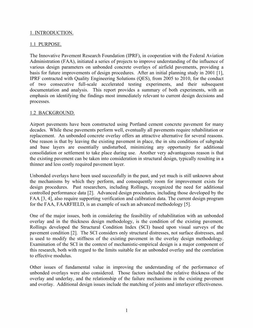
The CBR test results show a similar trend to that from the plate load test data. In test items N2 and S2, the post-testing CBR values are slightly lower than the preconstruction results. For the remaining test items, the post-testing CBR is very slightly higher than the average preconstruction CBR for that structural cross-section. Test items N2 and S2 had the highest mean preconstruction CBR, with the highest values occurring near the east end of the test items.

16

The vane shear test results in figure 9 indicate lower values measured at the surface of the subgrade after loading, as compared with the preconstruction mean values. However, the data show an increase at the 6-inch depth relative to the surface measured values, consistently exceeding even the preconstruction means. From this information, several summary remarks about the observed effects of loading on the subgrade can be made:

• The post-loading modulus of subgrade reaction values were lower than the preconstruction values for all test items. However, in most cases, those values were higher than the k values for plate load tests conducted on the subgrade under the unloaded transition slabs.

• The CBR tests show slightly less location-related variation in the subgrade stiffness, but

are mean values not single location tests. Generally, these test results indicate greater stiffness after testing than prior to, except the mean value for test items N2 and S2 that was high relative to other measurements.

• After load-testing, vane shear test results show an increase in subgrade stiffness at a 6-

inch depth as compared with the subgrade surface. 2.4 LOADING. 2.4.1 Load Configurations. The test vehicle at the NAPTF is designed to simulate actual aircraft loading. The test vehicle is equipped with two loading modules, each of which is configurable to different gear configurations of aircraft tires. For the unbonded overlay experiments, the north test items (N1, N2, N3) were loaded with the triple dual tandem, and the south test items (S1, S2, S3) were loaded with the twin dual tandem. The gear configurations are illustrated in figure 10. These configurations have equal axle and tire spacings, and do not precisely replicate any specific aircraft gear, but rather are generic configurations for purposes of comparison. The speed of the test vehicle for this study was fixed at three miles per hour. For the Baseline Experiment, the wheel load for failure loading was 50,000 lbs per wheel. For the SCI Validation Study, the wheel load was 42,500 lbs per wheel. The vehicle wander pattern consisted of 66 passes arranged in 9 wheel tracks, as summarized in table 6. The distance between each wheel track was 10.25 inches for all loading conducted in this project, providing a standard deviation similar to that measured on airfield taxiways. The load positions for both gears for track 0 are shown in figure 11, relative to the overlay and underlay joint positions. The outside tire of each gear was aligned adjacent to the overlay joint within the test items.

17

FIGURE 10. GEAR CONFIGURATIONS FOR THE TRIPLE DUAL TANDEM (LEFT) AND

TWIN DUAL TANDEM (RIGHT)

TABLE 6. WANDER PATTERN DIAGRAMS AND LOADING LOCATIONS

Track Frequencies 6.1% 9.1% 12.1% 15.2% 15.2% 15.2% 12.1% 9.1% 6.1%

Normal Distribution σ = 30.5 in

63,64 65,66 61,62 51,52 59,60 53,54 57,58 55,56 43,44 45,46 41,42 47,48 39,40 49,50 37,38

19,20 35,36 21,22 33,34 23,24 31,32 25,26 29,30 27,28

Wander Pattern Diagram

1,2 17,18 3,4 15,16 5,6 13,14 7,8 11,12 9,10 Track Number -4 -3 -2 -1 0 1 2 3 4 North Loading Centerline Location (ft) -18.167 -17.313 -16.458 -15.604 -14.750 -13.896 -13.042 -12.188 -11.333

South Loading Centerline Location (ft) 11.333 12.188 13.042 13.896 14.750 15.604 16.458 17.313 18.167

18

FIGURE 11. LOADING POSITION RELATIVE TO UNDERLAY (DASHED) AND OVERLAY (SOLID) JOINTS FOR ZERO TRACK

2.4.2 Progress of Loading. Loading for the two experimental phases occurred in 2006, 2007, and 2008, as was shown in table 5. Each experiment began with response loading at progressively-increasing wheel loads. The purpose of that loading was to make sure all systems were operating properly, and to assist in making the final decision about the wheel load to be used for the failure loading. Failure loading of the Baseline Experiment was conducted from July 25, 2006 to October 31, 2006, at wheel loads of 50,000 pounds. Failure loading of the SCI Validation Study was conducted from October 24, 2007 to April 15, 2008, at wheel loads of 42,500 pounds. Loading of the pavement test sections proceeded at the final wheel load levels for both experiments. As planned, the north test items were loaded with the triple dual tandem, and the south test items with the dual tandem gear configuration. Loading for the Baseline Experiment

Overlay Strain Gage

Underlay Strain Gage

Overlay LPT

Underlay LPT

19

continued until each section developed an approximate SCI of 20 or less, in an attempt to obtain a pattern of intersecting cracks, as documented in chapter 3. For the SCI Validation Study, some test items retained a higher SCI after over 40,000 passes, and loading was terminated. The cumulative load passes applied to each experiment test items are listed in tables 7 and 8.

TABLE 7. CUMULATIVE LOAD PASSES FOR BASELINE TESTING DATES

Date

Cumulative Passes,

North Test Items

Cumulative Passes,

South Test Items

Date

Cumulative Passes,

North Test Items

Cumulative Passes,

South Test Items

7/25/2006 132 132 9/20/2006 5146 6928 7/26/2006 528 528 9/21/2006 5146 7588 7/27/2006 924 924 9/22/2006 5146 8116 7/28/2006 1188 1188 9/25/2006 5146 8776 7/31/2006 1782 1782 9/26/2006 5146 9370 8/1/2006 2046 2046 9/27/2006 5146 9766 8/2/2006 2244 2244 9/28/2006 5146 10426 8/3/2006 2574 2706 9/29/2006 5146 11020 8/4/2006 2574 3168 10/2/2006 5146 11614 8/7/2006 2574 3432 10/3/2006 5146 12142 8/9/2006 2574 3894 10/11/2006 5146 12538

8/10/2006 2772 4356 10/12/2006 5146 13132 8/11/2006 3234 4818 10/13/2006 5146 13594 8/24/2006 3234 4950 10/16/2006 5146 14056 8/25/2006 3234 5016 10/17/2006 5146 14270 9/14/2006 3744 5016 10/26/2006 5146 14337 9/15/2006 3744 5526 10/30/2006 5146 15509 9/18/2006 4024 5806 10/31/2006 5146 16567 9/19/2006 4552 6334

20

TABLE 8. CUMULATIVE LOAD PASSES FOR SCI TESTING DATES

Date Cumulative Passes Date Cumulative

Passes Date Cumulative Passes

10/23/2007 198 12/14/2007 10032 3/3/2008 23628 10/24/2007 396 12/17/2007 10494 3/4/2008 24194 10/25/2007 594 12/18/2007 10858 3/5/2008 24684 10/26/2007 726 12/19/2007 11286 3/6/2008 25344 10/29/2007 924 12/20/2007 11682 3/7/2008 25938 10/30/2007 1122 12/21/2007 11814 3/10/2008 26466 10/31/2007 1386 1/8/2008 11880 3/11/2008 27126 11/1/2007 1716 1/9/2008 12210 3/12/2008 27588 11/2/2007 1980 1/10/2008 12870 3/13/2008 27918 11/5/2007 2376 1/11/2008 13398 3/14/2008 28078 11/6/2007 2640 1/14/2008 13926 3/17/2008 28710 11/7/2007 2970 1/15/2008 14322 3/18/2008 29238 11/9/2007 3168 1/16/2008 14850 3/19/2008 29436

11/13/2007 3432 1/17/2008 15246 3/20/2008 30096 11/14/2007 3696 1/18/2008 15510 3/21/2008 30756 11/15/2007 4026 1/22/2008 16038 3/24/2008 31350 11/19/2007 4422 1/23/2008 16316 3/25/2008 31944 11/20/2007 4818 1/24/2008 16962 3/26/2008 32604 11/21/2007 4950 1/25/2008 17490 3/27/2008 33264 11/26/2007 5214 1/28/2008 17952 3/28/2008 33858 11/27/2007 5610 1/30/2008 18084 3/31/2008 34386 11/28/2007 6006 1/31/2008 18480 4/1/2008 34980 11/29/2007 6402 2/1/2008 19008 4/2/2008 35260 11/30/2007 6798 2/4/2008 19602 4/3/2008 36036 12/3/2007 7194 2/5/2008 19937 4/4/2008 36512 12/4/2007 7590 2/20/2008 19932 4/7/2008 37040 12/5/2007 7986 2/21/2008 20064 4/8/2008 37818 12/6/2007 8382 2/25/2008 20328 4/9/2008 38544 12/7/2007 8712 2/26/2008 20988 4/10/2008 39666

12/10/2007 9108 2/27/2008 21648 4/11/2008 40854 12/11/2007 9504 2/28/2008 22308 4/14/2008 42174 12/13/2007 9900 2/29/2008 22968 4/15/2008 42834

2.5 MONITORING AND TESTING. 2.5.1 Watering. Within the indoor test facility, the concrete pavement test sections were not exposed to daily moisture changes typical of rain cycles at most airports. In order to counteract the curling/warping effects on the concrete pavement caused by the lack of moisture in the building,

21

the NAPTF personnel watered the test items. The monitoring protocols and watering frequency were based upon previous studies at the NAPTF [7]. Watering took place twice a week following curing of the Baseline Experiment and SCI Validation Study, and continued until the completion of loading and final deflection testing for both experiments. Slab corner upward movements were also monitored with the LPT gages, and watering was triggered any time corner uplift approached 60 mils. 2.5.2 Distress Surveys. Distress surveys were conducted prior to the load testing, and at regular intervals throughout the experiments. Distress surveys were conducted by the on-site engineers under the employ of the FAA during the Baseline Experiment and from QES during the SCI Validation Study. Distress surveys were performed at varying intervals during the Baseline Experiment, and each time the on-site engineer observed a new or expanded crack during the SCI Validation Study. Prior to the surveys, the pavement was carefully swept. When possible, the surveys were conducted when the pavement surface was still minimally damp from the slab watering as the cracks dried more slowly than the intact slab surface. As needed, the surveys were augmented with wire brushes, chalk markings, flashlights, magnifying glasses and other tools needed to ascertain the presence and pattern of very fine cracks. Due to the relatively stable indoor environment, most of the cracks remained very tight, increasing the survey difficulty. All distresses were measured and carefully mapped onto a field observation sheet before being logged electronically in a spreadsheet file. By tracking the progress of cracking patterns on a day-to-day basis, monitoring of the strain gages was able to be focused to relay any observed data reactions to the investigative team, and SCI values for each test item could be tracked. At the conclusion of loading for all test items, a final distress survey was performed. This final distress survey included all cracks visible at the end of loading to be used as a complete hand-drawn record of the final cracking pattern of the test pavements. 2.5.3 Response Monitoring. Data acquisition from the embedded instruments began immediately after construction of the overlay pavements. Data was collected through two data acquisition boxes (identified as SPU3 and SPU4), each with three cards. In addition, the thermistor data sets, which are entirely static (not load-dependent), were collected separately with a multiplexor, and supplied by the FAA in spreadsheet files. During loading, data sets from each SPU card were stored in a separate file for each load pass. Between loading periods, data was collected at regular time intervals, typically every hour, so that changes due to environmental conditions could be monitored. The dynamic responses of the instrumentation to loading were collected with each load pass, and the strain gages were monitored daily for selected passes. The monitoring of these responses sometimes showed a change in magnitude or pattern of response prior to selected observed distresses. However, the strain gage responses and dynamic responses of the LPTs were primarily used for analysis after the conclusion of the testing.

22

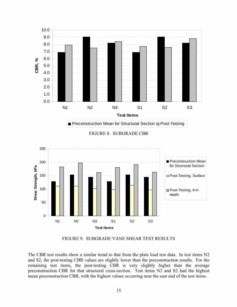
The FAA provided the loading period data as raw data files, and also provided a program for the conversion of the files to processed voltages or to engineering units; that program is called “TenView,” as the responses from 10 gages can be viewed on the screen at once. The TenView program was utilized directly for the monitoring of responses during the experiments. For subsequent data analysis, selected files were processed with TenView and full data sets stored in Excel. Spreadsheet macros were then developed for extracting the needed values. This procedure required each individual file to be processed separately using the series of programs. The development of a complete database of all responses is beyond the scope of the IPRF project. 2.5.4 Heavy Weight Deflectometer Testing. The FAA conducted heavy falling weight deflectometer (HWD) testing at requested intervals using a KUAB HWD. The HWD testing was conducted with a four-drop loading sequence, at all locations, beginning with an approximate 36,000-lb seating load. The subsequent loads were approximately 12,000 lbs, 24,000 lbs, and 36,000 lbs. The planned Baseline Experiment HWD testing pattern was painted on the pavement, as shown in figure 12. This testing plan included extensive joint and corner testing. The joint load transfer values did not change quickly over time, and the collection of this data was very time consuming. In addition, the planned testing pattern did not include center slab testing on all slabs. The center slab testing, which could be used for backcalculation of modulus values, and for monitoring the changing support conditions, was determined to be of greater value during the course of the Baseline Experiment. Therefore, as the experiment progressed, fewer load transfer tests were performed, and all center slabs were tested on a more frequent basis. The expanded HWD testing plan that was utilized for later testing is shown in figure 13. Using results and lessons learned from the Baseline Experiment, the SCI Validation Study HWD testing plan included a balanced mix of joint load transfer testing and center slab testing, as illustrated in figure 14. A more comprehensive testing plan with greater testing coverage was performed at critical milestones. This testing plan included extensive joint and corner testing, as shown in figure 15.

23

FIGURE 12. STANDARD BASELINE HWD TESTING

24

FIGURE 13. EXPANDED BASELINE EXPERIMENT HWD TESTING

25

FIGURE 14. STANDARD SCI VALIDATION STUDY HWD TESTING

26

FIGURE 15. EXPANDED SCI VALIDATION STUDY HWD TESTING

27

3. DATA AND PRELIMINARY ANALYSIS. In addition to the construction and materials information summarized in chapter 2, the data collected during Baseline Experiment and SCI Validation Study full-scale accelerated testing experiments at the NAPTF included distress, HWD results, instrumentation responses, and test vehicle and profile information. This chapter provides a summary of the processed distress and deflection data. Examples of the summarized instrumentation data included in the project research reports are also provided. The instrumentation data provides a resource for further analysis beyond the scope of this project. 3.1 DISTRESS. 3.1.1 Distress Maps. As described in the previous chapter, distress surveys of the unbonded overlays in both experiments were conducted at regular intervals after cracking was initiated. The dates of first observed crack for both the Baseline Experiment and the SCI Validation Study are shown in table 9. In addition, distress surveys were conducted for the underlay slabs during the intervals when they were exposed—prior to the initial Baseline Experiment overlay, after removal of the Baseline Experiment Overlay, after direct loading prior to the SCI Validation Study overlay, and after removal of the SCI Validation Study overlay. All surveys were conducted according to the provisions of ASTM D 5340-03 Airport Pavement Condition Index Surveys [8].

TABLE 9. FIRST LOADING DATE AND FIRST CRACK OBSERVATION DATE

Baseline Experiment SCI Validation Study First Loading Date: 7/25/06 First Loading Date: 10/23/07

Test Item First Crack Date Test Item First Crack Date N1 8/1/2006 N1 11/14/2007 N2 8/1/2006 N2 12/3/2007 N3 8/1/2006 N3 12/5/2007 S1 8/4/2006 S1 12/13/2007 S2 8/8/2006 S2 1/23/2008 S3 8/4/2006 S3 1/22/2008

The full set of final distress maps, showing the final condition of the test items after each phase of construction and loading, is included in figures 16 through 30. These 15 figures, together with the supporting structure and loading information, are the primary direct experimental result from the full-scale accelerated testing, and, therefore, are provided in full for visual reference. Detailed examination of the figures can be time-consuming, but can also provide the basis for significant observations. Consideration of the relative types and quantities of distresses in these visual representations, as compared to field pavements, can provide one element of support for implementing the experimental findings into design decisions.

28

FIGURE 16. DISTRESS SURVEY ON BASELINE OVERLAY AFTER FINAL LOADING FOR TEST ITEMS N1 AND S1

29


30


31

FIGURE 19. DISTRESS SURVEY ON BASE SLAB AFTER REMOVAL OF BASELINE OVERLAY FOR TEST ITEMS N1 AND S1

32

FIGURE 20. DISTRESS SURVEY ON UNDERLYING SLAB AFTER REMOVAL OF BASELINE OVERLAY FOR TEST ITEMS N2 AND S2

33

FIGURE 21. DISTRESS SURVEY ON UNDERLYING SLAB AFTER REMOVAL OF BASELINE OVERLAY FOR TEST ITEMS N3 AND S3

34

FIGURE 22. DISTRESS SURVEY ON UNDERLYING SLAB AFTER REMOVAL OF BASELINE OVERLAY AND ADDITIONAL LOADING FOR TEST ITEMS N1 AND S1

PRIOR TO PLACEMENT OF SCI OVERLAY

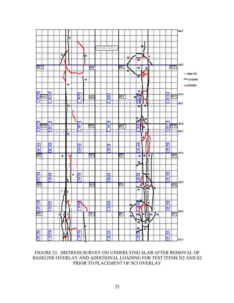
35



36



37

FIGURE 25. DISTRESS SURVEY ON SCI OVERLAY AFTER FINAL LOADING FOR TEST ITEMS N1 AND S1

38


39


40

FIGURE 28. DISTRESS SURVEY ON SCI UNDERLAY AFTER FINAL LOADING AND REMOVAL OF SCI OVERLAY FOR TEST ITEMS N1 AND S1

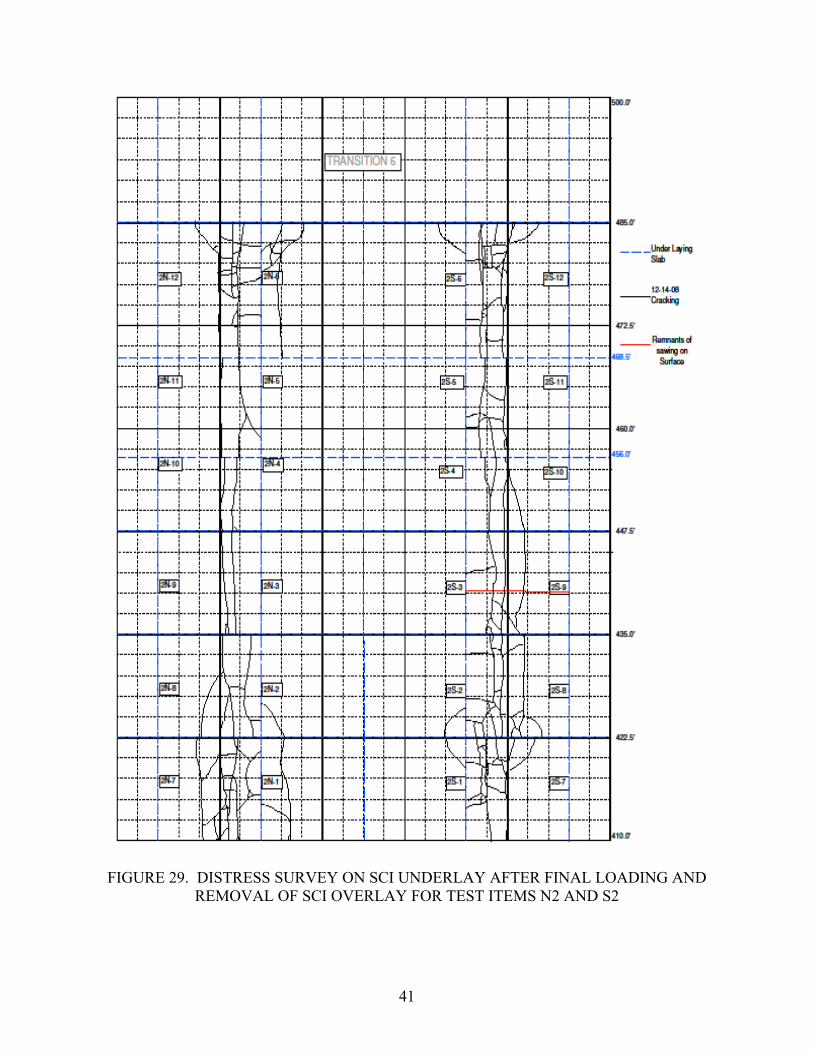
41


42


43

3.1.2 Distress Observations. During the Baseline Experiment, with the intact underlying slabs, the initial cracks were longitudinal, and longitudinal cracking continued to predominate as the overlay deteriorated, as illustrated in figures 16 through 18. Loading was continued to a more-distressed condition than originally planned in order to observe this progression of distress. The first cracks to be observed were outside (or near the outside) of the loaded area, and were confirmed to be top-down cracks by coring in the transition zone. But those cracks were followed almost immediately by bottom-up cracks within the loaded slabs. As summarized in Operational Life of Airport Pavements [9], top-down cracking is typically expected only in larger slabs and when curling is significant, and is also expected to appear in the form of corner breaks. A similar cracking pattern was observed during previous accelerated testing, and the causative conditions have been thoroughly examined but not yet fully explained using finite element analysis [10, 11] Upon removal of the overlay and interlayer, the cracking pattern in the underlay was also observed to be predominantly longitudinal, as shown in figures 19 through 21. In every case, the underlay exhibited somewhat less cracking than the overlay above, although this was most pronounced for the thicker underlying slabs. The areas with more intersecting crack patterns were directly below the similar areas in the overlay. Observations and sketches made during the overlay and interlayer deconstruction indicated that the overlay and underlay cracks did not directly line up, but were offset. That is, cracks did not appear to directly progress through the asphalt concrete interlayer. After completion of the Baseline Experiment, the underlying slabs were left in place to serve as the underlay for the SCI Validation Study. No pre-overlay repairs were made. In an attempt to make the slab support conditions more uniform within test items N1 and S1, load passes at reduced load levels were applied directly to only the less-distressed slabs. However, this resulted in the appearance of additional visible cracks within the unloaded slabs as well. To produce a distribution of support conditions, the remaining test items were also loaded directly on all slabs. The resulting pre-overlay distress surveys were provided in figures 22 through 24. During the SCI Validation Study, the first cracks to appear were again longitudinal. However, the longitudinal cracking pattern did not predominate, particularly for the test items with the most-distressed underlying slabs. The distress pattern was sympathetic to the underlying distresses in test items N1, S1, and N2. For test item S2, due to time constraints, loading was stopped before all slabs were distressed. The distresses that did appear were concentrated in the end slabs, which also had more distress below. The distress surveys on the SCI Validation Study overlay slabs were summarized in figures 25 through 27. Upon removal of the SCI Validation Study overlay, distress surveys were again conducted on the underlay slabs, and are shown in figures 28 through 30. In contrast to the Baseline Experiment, the underlay test items were distressed as much or more than the overlying slabs, except for test items N3 and S3, which had minimal pre-overlay cracking. The cracking patterns in the N1, S1, N2, and S2 underlays progressed from their previous pattern. The cracking patterns in the N3 and S3 underlay slabs were predominantly longitudinal and very concentrated under the most heavily-loaded area.

44

3.1.3 Structural Condition Index. The Pavement Condition Index (PCI) is a numerical indicator used to rate the surface condition of the pavement, and is used widely in pavement management. PCI is scaled from 0 to 100 based on the density and severity of defined distress types (15 types for rigid pavement). PCI is defined in ASTM D5340 as:

PCI =100 − a f (Ti,S j ,Dij )j=1

n

∑i=1

m

∑ (1)

Factor “a” is an adjustment factor depending on the number of distress types with deduct values in excess of five points (this factor was necessary to match the original engineer panel's ratings); m is total number of distress types; n is total number of severity levels for each distress type; and f (Ti,S j ,Dij ) is deduct value for distress type Ti, at severity level Sj existing at density Dij.

A modified index that is only concerned with structural distresses, SCI, was first introduced by Rollings in 1988 for airfield rigid pavement design [2]. SCI is defined as:

SCI =100− a f (Ti,S j ,Dij )j=1

n

∑i=1

m

∑ (2)

where SCI = Structural Condition Index and Ti = structural-related distress type The SCI calculation procedure is summarized below:

1. Determine the pavement sample unit: ASTM D5340 indicates that a pavement section selected for SCI calculation should have a standard size range of 20 contiguous slabs (±8 slabs to accommodate site-specific conditions. The experimental test items each consisted of 12 slabs, and are treated as a sample unit. The small sample unit size causes the SCI to drop in larger increments, but the size is within the limits.

2. Identify distress type and severity within one pavement sample unit: Distress types and severity are determined according to the definitions in ASTM D5340.

3. Distress density calculation within one pavement sample unit and corresponding deduct value determination: After determining the distress types and corresponding severities, distress density is calculated based on the percentage of slabs with the test item exhibiting a specific distress type at one severity. For example, if 6 slabs within the same sample unit (12 slabs) display low-severity corner breaks, the density of the low-severity corner break is 50%. The density of each distress type at different severity levels was calculated and the corresponding deduct values determined (deduct charts provided in ASTM D5340).

4. Determine corrected deduct value (CDV) and final SCI: After calculating the deduct values for all distresses, the procedure in ASTM D5340 is used to determine the maximum CDV. The final SCI of the pavement sample unit is 1 – max. CDV.

45

SCI was calculated for each test item for each time period that distress surveys were performed. Probably due to the environmental and accelerated characteristics of the indoor experiment, no distresses of high severity were observed, and only specific combinations of distresses were, therefore, used for the SCI calculations. The distress combinations observed in the Baseline Experiment and SCI Validation Study are summarized in table 10. The shrinkage crack definition is used in the SCI to describe smaller structural cracks, not for true shrinkage cracks. A spreadsheet macro was developed and verified to facilitate the consistent calculation of overlay SCI. All SCI calculations were independently verified from the distress survey maps and notes.

TABLE 10. DISTRESS COMBINATIONS OBSERVED IN UNBONDED OVERLAY EXPERIMENTS

Crack Type (Severity) Shrinkage (L) LDT (L) LDT (L) + Shrinkage (L) Corner Break (L) Corner Break (L) + Shrinkage (L) Corner Break (M) + Shrinkage (L) LDT (L) + Corner Break (L) Shattered Slab (L) Shattered Slab (M) LDT (L) + Corner Break (L) + Shrinkage (L) LDT (L) + Corner Break (M) LDT (L) + Corner Break (M) + Shrinkage (L)

Table 11 lists the overlay SCI versus passes for the Baseline Experiment, while table 12 lists the overlay SCI versus passes for the SCI Validation Study. The decrease in SCI versus passes (or coverages) is an important performance predictor in airfield rigid pavement design and is further discussed in chapter 4. SCI was also calculated from the distress surveys on the underlay slabs, as shown in table 13. In the underlay, the offset longitudinal joints produced a somewhat different slab configuration, with a row of narrow slabs along the edge and outside of the loaded area. For consistency, however, the SCI was still computed for 12 slabs within each test item.

46

TABLE 11. BASELINE DATE, CUMULATIVE PASSES, AND OVERLAY SCI

N1 S1 N2 S2 N3 S3 Date SCI Passes SCI Passes SCI Passes SCI Passes SCI Passes SCI Passes

7/25/2006 100 132 100 132 100 132 100 132 100 132 100 1328/1/2006 100 2046 100 2046 100 2046 100 2046 100 2046 100 20468/3/2006 80 2456 100 2456 74 2456 100 2456 99 2456 100 24568/4/2006 73 2574 93 3168 67 2574 100 3168 91 2574 86 31688/8/2006 73 2574 85 3432 67 2574 100 3432 75 2574 75 34328/9/2006 73 2574 78 3762 67 2574 100 3762 75 2574 70 3762

8/10/2006 73 2772 76 4356 67 2772 99 4356 75 2772 64 43568/11/2006 68 3234 67 4818 60 3234 98 4818 74 3234 55 48188/24/2006 63 3234 67 4818 54 3234 90 4818 57 3234 55 48188/28/2006 57 3234 67 5016 54 3234 90 5016 57 3234 52 50169/13/2006 46 3234 54 5016 54 3234 90 5016 57 3234 48 50169/14/2006 39 3742 51 5524 45 3742 80 5524 51 3742 41 55249/19/2006 31 4088 50 5870 38 4088 79 5870 44 4088 35 58709/22/2006 24 5146 46 8116 27 5146 76 8116 32 5146 35 81169/26/2006 19 5146 32 9370 27 5146 64 9370 29 5146 28 93709/29/2006 19 5146 22 11020 24 5146 48 11020 29 5146 28 1102010/2/2006 16 5146 16 11614 21 5146 48 11614 29 5146 24 1161410/3/2006 14 5146 7 12142 21 5146 40 12142 29 5146 15 12142

10/12/2006 12 5146 7 12142 21 5146 29 13132 29 5146 15 1214210/16/2006 12 5146 7 12142 21 5146 20 14056 29 5146 15 1214210/31/2006 12 5146 7 12142 21 5146 17 16567 29 5146 15 12142

47

TABLE 12. SCI OVERLAY DATE, CUMULATIVE PASSES, AND OVERLAY SCI

N1 S1 N2 S2 N3 S3 Date

SCI Passes SCI Passes SCI Passes SCI Passes SCI Passes SCI Passes

10/23/2007 100 198 100 198 100 198 100 198 100 198 100 19811/13/2007 100 3432 100 3432 100 3432 100 3432 100 3432 100 343211/14/2007 88 3696 100 3696 100 3696 100 3696 100 3696 100 369611/19/2007 83 4422 100 4422 100 4422 100 4422 100 4422 100 442211/21/2007 77 4950 100 4950 100 4950 100 4950 100 4950 100 495012/3/2007 68 7194 100 7194 88 7194 100 7194 100 7194 100 719412/5/2007 55 7986 100 7986 83 7986 100 7986 85 7986 100 798612/7/2007 51 8712 100 8712 83 8712 100 8712 85 8712 100 8712

12/10/2007 48 9108 100 9108 83 9108 100 9108 85 9108 100 910812/11/2007 42 9504 100 9504 83 9504 100 9504 85 9504 100 950412/13/2007 42 9900 88 9900 76 9900 100 9900 85 9900 100 990012/21/2007 27 11814 88 11814 76 11814 100 11814 85 11814 100 118141/11/2008 26 13398 88 13398 70 13398 100 13398 77 13398 100 133981/16/2008 24 14850 80 14850 70 14850 100 14850 72 14850 100 148501/18/2008 12 15510 80 15510 64 15510 100 15510 70 15510 100 155101/22/2008 12 15510 80 16038 45 16038 100 16038 64 16038 93 160381/23/2008 12 15510 80 16316 45 16316 87 16316 45 16316 88 163161/25/2008 12 15510 80 17490 45 17490 87 17490 45 17490 88 17490

2/4/2008 12 15510 63 19602 45 19602 83 19602 42 19602 88 196022/26/2008 12 15510 58 20988 45 20988 83 20988 42 20988 88 209882/27/2008 12 15510 58 21648 37 21648 83 21648 42 21648 88 216482/28/2008 12 15510 58 22968 37 22968 83 22968 42 22968 82 22968

3/3/200 12 15510 58 23628 37 23628 78 23628 42 23628 82 236283/5/2008 12 15510 52 24684 37 24684 78 24684 42 24684 72 246843/6/2008 12 15510 52 25344 37 25344 78 25344 33 25344 65 25344

3/11/2008 12 15510 46 27126 37 27126 78 27126 31 27126 64 271263/18/2008 12 15510 43 29238 37 29238 78 29238 29 29238 63 292383/20/2008 12 15510 31 30096 37 30096 78 30096 29 30096 54 300963/21/2008 12 15510 29 30756 37 30756 78 30756 29 30756 54 307563/24/2008 12 15510 23 31350 37 31350 78 31350 29 31350 54 313503/26/2008 12 15510 20 32604 37 32604 78 32604 29 32604 50 326043/27/2008 12 15510 20 33132 37 33264 78 33264 29 33264 48 332643/31/2008 12 15510 20 33132 37 34386 75 34386 29 34386 48 34386

4/2/2008 12 15510 18 33132 29 35259 67 35259 27 35259 39 352594/15/2008 12 15510 18 33132 29 38346 66 42834 27 38346 39 38346

48

TABLE 13. UNDERLAY SCI COMPARISON BETWEEN BASELINE AND SCI OVERLAYS

Test Item SCI

Date N1 Underlay

S1 Underlay

N2 Underlay

S2 Underlay

N3 Underlay

S3 Underlay

7/25/2006 100 100 100 100 100 10012/18/2006 32 39 57 33 87 932/20/2007 25 23 43 28 84 81

12/14/2008 3 8 17 9 28 23 3.2 ANALYSIS OF DEFLECTION TESTING DATA. 3.2.1 Backcalculation of Layer Moduli. As described in chapter 2, KUAB HWD testing was conducted by the FAA during the course of both experiments. A number of backcalculation programs and sets of assumptions were used in evaluating the HWD data, and are described in the project research reports. This section describes the moduli backcalculation results obtained from use of the FAA’s BAKFAA program; those results are used in the subsequent analysis sections of this report. FAA personnel modified the BAKFAA program specifically for this project, to allow modeling of a thinner interlayer for backcalculation. A check on stability of the results for the thin interlayer was performed, and results found to be acceptable. The HWD deflection basins obtained at center slab locations under the heaviest load were used for backcalculation. BAKFAA uses the layered elastic analysis program LEAF, and minimizes the sum of the squares of difference between the measured and computed vertical deflections in order to find the best-fit set of moduli. Independent cross-checks by other team members, using the same input assumptions were performed for all backcalculations. The seed moduli and input assumptions used for the Baseline Experiment and SCI Validation Study are provided in tables 14 and 15, respectively. Modifications to these assumptions that were attempted included omitting the interlayer, changing the bonding conditions between layers, and fixing the subgrade modulus. The unbonded interface value (0) was used for all the interfaces with the underlying subbase and subgrade, which is less common than the assumption of the fully bonded condition for those layers (1). The physical reality of the interactions between layers may lie between the two input choices, depending upon loading and other factors. For these test conditions, the best correspondence, particularly in terms of consistency of results, was found for the assumptions shown in tables 14 and 15, and those results are used in the subsequent analyses. The backcalculations were performed with location-specific thicknesses, rather than average test item thicknesses; this was found to significantly improve the convergence and consistency of results.

49

During the SCI Validation Study backcalculations, the overlay modulus deteriorated rapidly as loads accumulated. As a result, the overlay seed modulus was lowered to 4000 ksi to assure the quality of the backcalculation results (lower RMS). Backcalculation results with RMS below 0.1 were considered valid and were documented.

TABLE 14. BAKFAA BASELINE SEED MODULI

LAYER E (ksi) ν INTERFACE PARAMETER

LAYER CHANGEABLE?

CONCRETE OVERLAY 4000 0.15 1 Yes ASPHALT INTERLAYER 200 0.40 0 Yes CONCRETE UNDERLAY 4000 0.15 0 Yes SUBBASE 40 0.45 0 Yes SUBGRADE 39.41 0.45 0 Yes

TABLE 15. BAKFAA SCI VALIDATION SEED MODULI

LAYER E (ksi) ν INTERFACE PARAMETER

LAYER CHANGEABLE

CONCRETE OVERLAY 7000/4000 0.15 1 Yes ASPHALT INTERLAYER 200 0.40 0 Yes CONCRETE UNDERLAY 2000 0.15 0 Yes SUBBASE 40 0.45 0 Yes SUBGRADE 39.41 0.45 0 Yes

Figures 31 through 42 show the complete history of backcalculated average moduli of layers for each test item across the time frames for both experiments. The moduli are the averages from center slab testing on the six loaded inner slabs in each test item. Summary observations include:

• The structural capacity of the overlay slab was fully “restored” by the replacement of the unbonded overlay. This simply provides a check on the reasonableness of the backcalculation results.

• The underlay slabs which remained in place continued to deteriorate, as anticipated. The

backcalculated moduli for these slabs are a key input to subsequent analysis of the required overlay design input parameters.

• The backcalculated moduli of the subgrade were reasonably constant across the course of

the experiment.

• The structural capacity of aggregate base and subgrade were apparently “restored” due to the application of the new unbonded overlay. This can be interpreted to be at least partially an artifact of the backcalculation assumptions, and of the reduced stress on the subgrade with the intact overlay condition.

50

0.0E+00

5.0E+06

1.0E+07

1.5E+07

132-

7/25

/06

1188

-7/2

8/06

2046

-8/1

/06

2574

-8/9

/06

3234

-8/1

5/06

5146

/10/

10/0

6

5146

/11/

7/06

0-8/

6/07

0-10

/22/

07

4026

-11/

16/0

7

1009

8-12

/14/

07

1181

4-12

/21/

07

1551

0-1/

23/0

8

1551

0-1/

31/0

8

1551

0-2/

22/2

008

1551

0-3/

13/0

8

1551

0-5/

29/0

8

Passes+Date

BA

KFA

A In

ner S

lab

Avg

. Mod

ulus

, psi

N1 Overlay Modulus N1 Underlay Modulus

FIGURE 31. BAKFAA BACKCALCULATION RESULTS, TEST ITEM N1, SLABS

0.0E+00

2.5E+04

5.0E+04

7.5E+04

132-

7/25

/06

1188

-7/2

8/06

2046

-8/1

/06

2574

-8/9

/06

3234

-8/1

5/06

5146

/10/

10/0

6

5146

/11/

7/06

0-8/

6/07

0-10

/22/

07

4026

-11/

16/0

7

1009

8-12

/14/

07

1181

4-12

/21/

07

1551

0-1/

23/0

8

1551

0-1/

31/0

8

1551

0-2/

22/2

008

1551

0-3/

13/0

8

1551

0-5/

29/0

8

Passes+Date

BA

KFA

A In

ner S

lab

Avg

. Mod

ulus

, psi

N1 Base Modulus N1 Subgrade Modulus

FIGURE 32. BAKFAA BACKCALCULATION RESULTS, TEST ITEM N1, BASE AND

SUBGRADE

51

0.0E+00

5.0E+06

1.0E+07

1.5E+07

132-

7/25

/06

1188

-7/2

8/06

2046

-8/1

/06

2574

-8/9

/06

3234

-8/1

5/06

5146

/10/

10/0

6

5146

/11/

7/06

0-8/

6/07

0-10

/22/

07

4026

-11/

16/0

7

1009

8-12

/14/

07

1181

4-12

/21/

07

1631

6-1/

23/0

8

1848

0-1/

31/0

8

2006

4-2/

22/0

8

2791

8-3/

31/0

8

3834

6-5/

29/0

8

Passes+Date

BA

KFA

A In

ner S

lab

Avg

. Mod

ulus

, psi



0.0E+00

2.5E+04

5.0E+04

7.5E+04

132-

7/25

/06

1188

-7/2

8/06

2046

-8/1

/06

2574

-8/9

/06

3234

-8/1

5/06

5146

/10/

10/0

6

5146

/11/

7/06

0-8/

6/07

0-10

/22/

07

4026

-11/

16/0

7

1009

8-12

/14/

07

1181

4-12

/21/

07

1631

6-1/

23/0

8

1848

0-1/

31/0

8

2006

4-2/

22/0

8

2791

8-3/

31/0

8

3834

6-5/

29/0

8

Passes+Date

BA

KFA

A In

ner S

lab

Avg

. Mod

ulus

, psi



SUBGRADE

52

0.0E+00

5.0E+06

1.0E+07

1.5E+07

132-

7/25

/06

1188

-7/2

8/06

2046

-8/1

/06

2574

-8/9

/06

3234

-8/1

5/06

5146

/10/

10/0

6

5146

/11/

7/06

0-8/

6/07

0-10

/22/

07

4026

-11/

16/0

7

1009

8-12

/14/

07

1181

4-12

/21/

07

1631

6-1/

23/0

8

1848

0-1/

31/0

8

2006

4-2/

22/0

8

2791

8-3/

31/0

8

3834

6-5/

29/0

8

Passes+Date

BA

KFA

A In

ner S

lab

Avg

. Mod

ulus

, psi



0.0E+00

2.5E+04

5.0E+04

7.5E+04

132-

7/25

/06

1188

-7/2

8/06

2046

-8/1

/06

2574

-8/9

/06

3234

-8/1

5/06

5146

/10/

10/0

6

5146

/11/

7/06

0-8/

6/07

0-10

/22/

07

4026

-11/

16/0

7

1009

8-12

/14/

07

1181

4-12

/21/

07

1631

6-1/

23/0

8

1848

0-1/

31/0

8

2006

4-2/

22/0

8

2791

8-3/

31/0

8

3834

6-5/

29/0

8

Passes+Date

BA

KFA

A In

ner S

lab

Avg

. Mod

ulus

, psi



SUBGRADE

53

0.0E+00

5.0E+06

1.0E+07

1.5E+07

132-

7/25

/06

1188

-7/2

8/06

2046

-8/1

/06

3894

-8/9

/06

4818

-8/1

5/06

1214

2/10

/10/

06

1214

2/11

/7/0

6

0-8/

7/07

0-10

/22/

07

4026

-11/

16/0

7

1009

8-12

/14/

07

1181

4-12

/21/

07

1631

6-1/

23/0

8

1848

0-1/

31/0

8

2006

4-2/

22/0

8

2791

8-3/

31/0

8

3326

4-5/

29/0

8

Passes+Date

BA

KFA

A In

ner S

lab

Avg

. Mod

ulus

, psi S1 Overlay Modulus S1 Underlay Modulus

FIGURE 37. BAKFAA BACKCALCULATION RESULTS, TEST ITEM S1, SLABS

0.0E+00

2.5E+04

5.0E+04

7.5E+04

132-

7/25

/06

1188

-7/2

8/06

2046

-8/1

/06

3894

-8/9

/06

4818

-8/1

5/06

1214

2/10

/10/

06

1214

2/11

/7/0

6

0-8/

7/07

0-10

/22/

07

1009

8-12

/14/

07

1181

4-12

/21/

07

1631

6-1/

23/0

8

1848

0-1/

31/0

8

2006

4-2/

22/0

8

2791

8-3/

31/0

8

3326

4-5/

29/0

8

Passes+Date

BA

KFA

A In

ner S

lab

Avg

. Mod

ulus

, psi

S1 Base Modulus S1 Subgrade Modulus

FIGURE 38. BAKFAA BACKCALCULATION RESULTS, TEST ITEM S1, BASE AND

SUBGRADE

54

0.0E+00

5.0E+06

1.0E+07

1.5E+07

132-

7/25

/06

1188

-7/2

8/06

2046

-8/1

/06

3894

-8/9

/06

4818

-8/1

5/06

1214

2/10

/10/

06

1748

9/11

/20/

06

0-8/

7/07

0-10

/22/

07

4026

-11/

16/0

7

1009

8-12

/14/

07

1181

4-12

/21/

07

1631

6-1/

23/0

8

1848

0-1/

31/0

8

2006

4-2/

22/0

8

2791

8-3/

31/0

8

4283

4-5/

29/0

8

Passes+Date

BA

KFA

A In

ner S

lab

Avg

. Mod

ulus

, psi S2 Overlay Modulus S2 Underlay Modulus


0.0E+00

2.5E+04

5.0E+04

7.5E+04

132-

7/25

/06

1188

-7/2

8/06

2046

-8/1

/06

3894

-8/9

/06

4818

-8/1

5/06

1214

2/10

/10/

06

1748

9/11

/20/

06

0-8/

7/07

0-10

/22/

07

4026

-11/

16/0

7

1009

8-12

/14/

07

1181

4-12

/21/

07

1631

6-1/

23/0

8

1848

0-1/

31/0

8

2006

4-2/

22/0

8

2791

8-3/

31/0

8

4283

4-5/

29/0

8

Passes+Date

BA

KFA

A In

ner S

lab

Avg

. Mod

ulus

, psi



SUBGRADE

55

0.0E+00

5.0E+06

1.0E+07

1.5E+07

132-

7/25

/06

1188

-7/2

8/06

2046

-8/1

/06

3894

-8/9

/06

4818

-8/1

5/06

1214

2/10

/10/

06

1214

2/11

/7/0

6

0-8/

7/07

0-10

/22/

07

4026

-11/

16/0

7

1009

8-12

/14/

07

1181

4-12

/21/

07

1631

6-1/

23/0

8

1848

0-1/

31/0

8

2006

4-2/

22/0

8

2791

8-3/

31/0

8

3834

6-5/

29/0

8

Passes+Date

BA

KFA

A In

ner S

lab

Avg

. Mod

ulus

, psi

S3 Overlay Modulus S3 Underlay Modulus


0.0E+00

2.5E+04

5.0E+04

7.5E+04

132-

7/25

/06

1188

-7/2

8/06

2046

-8/1

/06

3894

-8/9

/06

4818

-8/1

5/06

1214

2/10

/10/

06

1214

2/11

/7/0

6

0-8/

7/07

0-10

/22/

07

4026

-11/

16/0

7

1009

8-12

/14/

07

1181

4-12

/21/

07

1631

6-1/

23/0

8

1848

0-1/

31/0

8

2006

4-2/

22/0

8

2791

8-3/

31/0

8

3834

6-5/

29/0

8

Passes+Date

BA

KFA

A In

ner S

lab

Avg

. Mod

ulus

, psi



SUBGRADE

56

3.2.2 Load Transfer Efficiency. Load transfer efficiency (LTE) is important in rigid pavement design since it represents the ability of a rigid pavement to transfer a load across joints. Due to the time-consuming procedure of LTE deflection measurements within the confined space of the NAPTF, the LTE measurements were not taken after Aug. 16, 2006 in the Baseline Experiment, but were taken at regular intervals in the SCI Validation Study. Average deflection LTE is used to demonstrate the load transfer ability of matched and mismatched joints within a test item and to compare the load transfer abilities of different test items with time. Deflection LTE is defined as the percentage ratio between D1 (300 mm from the load center) and D0 (0 mm from the load center). Figures 43 and 44 show the variability of LTE at matched and mismatched joints within different test items over time. Observations about the calculated load transfer efficiencies include:

• The overlay procedure restores the LTE, as anticipated. It can be seen in the SCI Validation experiment that the LTE drops with time, as it is subjected to loading.

• The LTE at mismatched joints deteriorated less compared to LTE at matched joints

within the same test item.

• The lowest LTE occurred during December and February, which might be an effect of low-temperature slab contraction, effectively opening the joints.

3.3 INSTRUMENTATION RESPONSES. The instrumentation was used for monitoring during the loading, and the resulting data also provide a resource for post-experimental analysis. Much of that instrumentation data analysis is beyond the scope of the IPRF projects, but a significant subset of the data has been processed and evaluated, and is discussed in further detail in the other project reports [12, 13, 14]. During periods of non-loading, the static responses were recorded at regular intervals. During loading, the responses were recorded during each pass. 3.3.1 Static Responses (Temperature and LPTs). The Baseline Experiment and SCI Validation Study were constructed at similar dates. This overlap in dates, but in different years, provides an additional basis along with the indoor location, to assume similar environmental conditions for the two experiments. Figure 45 shows the mid-slab concrete temperatures for test item N1 from the Baseline Experiment and SCI Validation Study overlays. Figure 45 is plotted for the same dates, within the experiments’ respective years of construction.

57

20

30

40

50

60

70

80

90

100

3/24/06 7/2/06 10/10/06 1/18/07 4/28/07 8/6/07 11/14/07 2/22/08 6/1/08 9/9/08Dates

Avg

Def

lect

ion

LTE,

%

N1-Matched

N2-Matched

N3-Matched

N1-Mismatched

N2-Mismatched

N3-Mismatched

FIGURE 43. LOAD TRANSFER EFFICIENCY FOR NORTH TEST ITEMS

. Baseline . SCI Validation . No Measurement

58

20

30

40

50

60

70

80

90

100

3/24/06 7/2/06 10/10/06 1/18/07 4/28/07 8/6/07 11/14/07 2/22/08 6/1/08 9/9/08Dates

Avg

Def

lect

ion

LTE,

%

S1-Matched

S2-Matched

S3-Matched

S1-Mismatched

S2-Mismatched

S3-Mismatched

FIGURE 44. LOAD TRANSFER EFFICIENCY FOR SOUTH TEST ITEMS

. Baseline . SCI Validation . No Measurement

59

0

10

20

30

40

50

60

70

80

90

100

3/29 4/5 4/12 4/19 4/26 5/3 5/10Date

Tem

pera

ture

(°F)

BaselineSCI

FIGURE 45. TEMPERATURE COMPARISON FOR TEST ITEM N1 OVERLAY, FOR YEARS OF CONSTRUCTION

The Baseline Experiment and SCI Validation Study pavements, located indoors, were not exposed to normal rainfall cycles. Therefore, low moisture levels in the slabs may result in warping of the slab corners, as previous NAPTF studies have shown. In order to gauge the magnitude of the warping of the slab corners, linear position transducers were placed at the four corners and center of select concrete slabs. Two of these slabs were N2-5 and N3-2. These slabs were selected to examine the curling/warping of slab corners relative to the center of the slabs. Figures 46 and 47 provide examples of the positions of the slab corners and centers. Additional plots are included in the research reports. All data points in the figures were selected at 5:00 a.m. and on days with consistent data to reduce the effect of time and poor data points. From the full set of graphs, two observations were made. First, the watering efforts to minimize curling/warping, as described in chapter 2, were generally successful. Second, the sensors that were located directly under the loading path exhibited a lower magnitude of curling/warping for both the Baseline Experiment and SCI Validation Study.

60

-25.00

-20.00

-15.00

-10.00

-5.00

0.00

5.00

10.003/23 4/12 5/2 5/22 6/11 7/1

Measurement Date (SCI 2007, Baseline 2006)

Elev

atio

n of

Sla

b C

orne

r Ver

sus

Slab

Cen

ter (

mils

, Neg

ativ

e Va

lues

Indi

cate

Upw

ard

Mov

emen

t) BaselineN2-5SCI N2-5

BaselineN3-2SCI N3-2

FIGURE 46. COMPARISON OF NORTHEAST SLAB CORNER ELEVATIONS FOR OVERLAY SLABS BETWEEN BASELINE AND SCI EXPERIMENTS

-30.00

-25.00

-20.00

-15.00

-10.00

-5.00

0.00

5.00

10.003/23 4/12 5/2 5/22 6/11 7/1

Measurement Date (SCI 2007, Baseline 2006)

Elev

atio

n of

Sla

b C

orne

r Ver

sus

Slab

Cen

ter (

mils

, Neg

ativ

e Va

lues

Indi

cate

Upw

ard

Mov

emen

t) BaselineN2-5

SCI N2-5

BaselineN3-2

SCI N3-2

FIGURE 47. COMPARISON OF SOUTHWEST SLAB CORNER ELEVATIONS FOR

OVERLAY SLABS BETWEEN BASELINE AND SCI EXPERIMENTS

61

3.3.2 Responses of Soil Pressure Cells. Five soil pressure cells were installed prior to construction of the Baseline Experiment underlay pavement slabs. The pressure cells remained in situ, and all functioning through at least a portion of the SCI Validation Study. Because the two experiments were conducted at different failure wheel load levels, the dynamic responses of instruments cannot be directly compared. However, using the data from the pre-loading at lower wheel load levels, and short-range linear interpolation/normalization, the responses were compared. An example is shown in figure 48, normalized to a 40,000-lb wheel load.

0

5

10

15

20

25

30

-4 -3 -2 -1 0 1 2 3 4Track Number

Mea

n So

il Pr

essu

re R

espo

nses

from

one

W

ande

r, N

orm

aliz

ed to

40k

whe

el lo

ad, p

si

SCI SP1 (N1) SCI SP2 (N1) SCI SP3 (N3) SCI SP4 (N3) SCI SP5 (S3)

Baseline SP1 (N1) Baseline SP2 (N1) Baseline SP3 (N3) Baseline SP4 (N3) Baseline SP5 (S3)

FIGURE 48. MEAN SOIL PRESSURE CELL RESPONSES BY LOADING TRACK, BASELINE AND SCI VALIDATION STUDY COMPARISON FROM RAMP-UP LOADING The responses in figure 48 are for the newly constructed overlays, before any cracking had initiated. For the same loading conditions, the soil pressures in the SCI Validation Study were significantly higher than in the Baseline Experiment. This observation is consistent with the damaged condition of the underlay slabs. This plot is consistent with the assumption made that if failure loading of the SCI Validation Study had occurred at the same wheel load as used for the Baseline Experiment that failure might have progressed too rapidly.

62

3.3.3 Dynamic Responses of LPTs and Embedded Strain Gages. The FAA program TenView was utilized for extracting gage data from the binary files during the Baseline Experiment and for monitoring during the SCI Validation Study. However, the extensive data set allowed examination of only a small amount of the responses, for selected passes and dates, in that manner.

For preliminary analysis of the instrumentation data after the SCI Validation Study testing was completed, the FAA provided the source code so that the TenView program could be modified. This allowed for more efficient batch processing of the data and extraction for spreadsheet analysis and plotting. MATLAB software was then utilized for subsequent analysis, including the computation of peak responses. MATLAB programming was used to remove the gage responses which were either bad or had no data. Also, it helped to automate the data interpretation as two responses from the same gage type at two different locations were not the same in pattern. Initially, portions of the gage response graphs were defined. The definitions used for the strain gages, for example, were as shown in figure 49.

FIGURE 49. DEFINITION OF RESPONSE COMPONENTS FOR EMBEDDED STRAIN GAGES (SHOWN AS MICROSTRAIN VERSUS NUMBER OF SAMPLING CYCLES)

Before the Baseline Experiment loading started on July 25, 2006, the cross-sections were preloaded with triple dual tandem and twin dual tandem gears at wheel loads in incremental increases, as described in the Baseline Experiment final report. The responses captured by the gages were used to check if the 0 track, when vehicle passes directly over the strain, yields the highest peak strain responses. Peak strain responses from all the gages were calculated for all passes from one wander pattern at a wheel load of 40,000 lbs (66 passes), and plotted as shown in figure 50, for example.

63

FIGURE 50. STRAIN GAGE AVERAGE RESPONSES FROM ONE WANDER OF RAMP-UP LOADING FOR GAGES IN TEST ITEM NORTH 1 WITH TRIPLE DUAL TANDEM

LOADING

Graphs such as those shown in figures 51 and 52 were prepared for all embedded strain gages and linear position transducers in both the Baseline Experiment and SCI Validation Study. Those plots were completed after the Baseline Experiment final report was completed, and are thus included in the appendices of the SCI Validation Study final research report. Figure 51 shows the responses from embedded strain gages in similar positions in test items N2 and S2 during the SCI Validation Study. The plotted responses are all from Track 0 passes, which typically produced the greatest strain magnitudes at the instrumentation locations. The plotted strains are the mean and two-standard-deviation range of all passes in Track 0 on the indicated dates.

64

-200

-150

-100

-50

0

50

100

150

200

0 5000 10000 15000 20000 25000 30000 35000 40000 45000

Total Passes

Trac

k 0

East

boun

d, m

icro

stra

in

EG-2-N2-1B (Daily Avg)EG-2-N2-1T (Daily Avg)EG-U-N2-1B (Daily Avg)EG-U-N2-1T (Daily Avg)

-200

-150

-100

-50

0

50

100

150

200

0 5000 10000 15000 20000 25000 30000 35000 40000 45000

Total Passes

Trac

k 0

East

boun

d, m

icro

stra

in

EG-2-S2-1B (Daily Avg)EG-2-S2-1T (Daily Avg)EG-U-S2-1B (Daily Avg)EG-U-S2-1T (Daily Avg)

FIGURE 51. SCI VALIDATION DAILY AVERAGE STRAIN GAGE RESPONSES WITH 2-

SD ERROR BARS, TRACK 0 EASTBOUND, SLABS N2-2, N2-8, S2-2, S2-8

OL Strain Gage UL Strain Gage

65

These graphs allow the direct comparison of the peak strain responses to the twin dual tandem and triple dual tandem gear. The difference in strain response between the overlay and underlay can be examined, as well as the magnitude of strain near the top and the bottom of a slab. It must be noted, however, that the strain gages may not have been located at the position of greatest strain within each slab. Several observations were made by examining the full set of these strain plots:

• The ratio in magnitude of peak strain produced by the triple dual tandem and twin dual

tandem gears is not inversely proportional to the number of passes until failure. The ratio of passes to reach a specified condition is greater than can be explained only by the peak magnitude of measured strains.

• For all ratios of underlay to overlay thickness, the peak strains were typically larger in the

overlay than underlay. This corresponds to the observed distress progression.

• The relative strains between the top and bottom gages at a location varied both by gage, and with the accumulation of loading passes and damage.

• The responses of some gages, and some dates, are significantly variable. Therefore,

examination of only randomly selected passes, even in the same track and at the same time of day, may produce erroneous conclusions.

Figure 52 shows the responses from linear position transducers in similar positions in test items N2 and S2 during the SCI Validation Study. The plotted responses are again from Track 0 passes. Initial responses of the gages were similar. The slower deterioration of the S2 test item is apparent, as the deflection responses were relatively constant over the course of the experiment. For test item N2, however, the deflections increased in both magnitude and variability as loading progressed.

66

0

25

50

75

0 5000 10000 15000 20000 25000 30000 35000 40000 45000

Total Passes

Trac

k 0

East

boun

d, m

ils

LPT-2-N2-8 (Daily Avg)



LPT-U-N2-3 (Daily Avg)

LPT-U-N2-4 (Daily Avg)

0

25

50

75

0 5000 10000 15000 20000 25000 30000 35000 40000 45000

Total Passes

Trac

k 0

East

boun

d, m

ils

LPT-2-S2-8 (Daily Avg)LPT-U-S2-3 (Daily Avg)LPT-U-S2-4 (Daily Avg)

FIGURE 52. SCI VALIDATION DAILY AVERAGE LPT RESPONSES WITH 2-SD ERROR

BARS, TRACK 0 EASTBOUND, SLABS N2-4, N2-5, S2-5

OL LPT UL LPT

67

4. OVERALL PERFORMANCE CURVES AND THICKNESS DESIGN COMPARISONS. 4.1 ADVISORY CIRCULAR 150 AND FAARFIELD. In 2009, the FAA issued Advisory Circular 150/5320-6E Airport Pavement Design and Evaluation, replacing AC 150/4320-6D, which was issued in 1995. For pavement design for airplanes weighing more than 30,000 pounds, the new advisory circular recommends mechanistic pavement design procedures. Those procedures are implemented in the FAA Rigid and Flexible Iterative Elastic Layer Design (FAARFIELD) program [13]. The new Advisory Circular and the FAARFIELD program are the latest steps in the implementation of mechanistic response models for airfield pavement design. The FAARFIELD rigid pavement design process considers only the cracking mode of failure for rigid pavements. FAARFIELD uses the maximum horizontal stress at the bottom edge of the concrete slab for an edge-loaded condition as the predictor of pavement structural life. In the Baseline Experiment and SCI Validation Study, the location of the embedded strain gages along the edge of the slabs, directly under the edge-loading gear in track 0 was intended to capture this condition. Fatigue failure is computed using Miner’s rule, expressed in terms of the cumulative damage factor (CDF). For a single loading condition, such as was applied during the Baseline Experiment and SCI Validation Study, the CDF is simply the ratio between the applied repetitions and the number of allowable repetitions to failure. At a CDF of 1, the pavement has used up its fatigue life. For overlay design of a pavement with no cracking, FAARFIELD utilizes the cumulative damage factor used to first crack (CDFU), which is defined as the amount of life of the existing pavement that has been used up to the time of the overlay. For rigid pavements, FAARFIELD utilizes a three-dimensional finite element model [4]. Overlay design is incorporated using the procedures that originated from Report DOT-FAA-PM-87/19, Design of Overlays for Rigid Airfield Pavements [2]. The deterioration of the existing rigid pavement must be determined, and is expressed in terms of SCI, as discussed in chapter 3. An SCI of 80 is defined as failure, and is consistent with half of the slabs in the traffic area having a structural crack, although that SCI value may be reached in other ways, depending upon a variety of pavement and loading factors. 4.2 UNBONDED OVERLAY DETERIORATION CURVES. 4.2.1 Performance Curves from the Experiments. In figures 53 and 54, the SCI values from each distress survey are plotted versus cumulative passes for each test item. These performance curves are a key product of this research, and a number of important observations can be obtained from them. Figure 53 illustrates the results of the Baseline Experiment, with plots on an arithmetic scale to differentiate the test item results, and on a logarithmic scale to correspond to traditional plotting of fatigue relationships.

68

0

10

20

30

40

50

60

70

80

90

100

0 5000 10000 15000 20000

Baseline Experiment Passes at 50,000-lb Wheel Load

Ove

rlay

SCI

N1

S1

N2

S2

N3

S3

0

10

20

30

40

50

60

70

80

90

100

100 1000 10000 100000

Baseline Experiment Passes at 50,000-lb Wheel Load

Ove

rlay

SCI N1

S1

N2

S2

N3

S3

FIGURE 53. BASELINE EXPERIMENT CUMULATIVE PASSES VERSUS SCI; ARITHMETIC SCALE (TOP) AND LOG SCALE (BOTTOM)

69

0

10

20

30

40

50

60

70

80

90

100

0 10000 20000 30000 40000 50000

SCI Validation Study Passes at 42,500-lb Wheel Load

Ove

rlay

SCI

N1

S1

N2

S2

N3

S3

0

10

20

30

40

50

60

70

80

90

100

100 1000 10000 100000

SCI Validation Study Passes at 42,500-lb Wheel Load

Ove

rlay

SCI

N1

S1

N2

S2

N3

S3

FIGURE 54. SCI VALIDATION STUDY CUMULATIVE PASSES VERSUS SCI; ARITHMETIC SCALE (TOP) AND LOG SCALE (BOTTOM)

70

The departure of the curves from the SCI = 100 portion would approximately represent the condition for which CDFU = 1, when the first crack would be observed. However, it may take some time to visually observe a crack, so the true occurence CDFU =1 may be earlier than the intercepts. The intercepts of the curves with SCI = 80 represent the conditions for which CDF = 1, consistent with the definition of failure for the new pavement.

In figure 53 for the Baseline Experiment, it can be seen that the South test items consistently required more passes to achieve a given SCI level than the North test items. This is consistent with the knowledge that gross aircraft weight is one of the most important factors in airfield pavement performance [9]. While both the North and South test items were loaded with a 50,000-lb wheel load, that produced a total load of 300,000 lb with the triple dual tandem on the North test items, and 200,000 lb with the twin dual tandem on the South test items. This is analagous to different size aircraft with gear configurations consistent with size.

The overlay deterioration rate was very similar between all three North test items in the Baseline Experiment in spite of the different overlay/underlay thickness ratios. The thin overlay over the thicker underlying pavement was the last to crack, and required slightly more passes to reach a predetermined (given) SCI level. Deterioration of the thin-over-thick and thick-over-thin South test items in the Baseline Experiment, was very similar. However, the South 2 test item, with approximately equal overlay and underlay thicknesses, required significantly more passes to reach a predetermined (given) SCI level.

Another perspective on the performance of the Baseline Experiment test items with various thickness ratios may be reached by considering the condition of the underlay after overlay removal. The terminal underlay conditions were provided in chapter 3, in figures 19 through 21, and in table13. The underlay slabs under the thick overlay were significantly cracked, with SCI values of 32 and 39, for N1 and S1, respectively. The underlay slabs under the thin overlay, however, had very little visible distress, with SCI values of 87 for test item N3 and 93 for test items S3. (These underlay slabs included one additional inch of thickness, relative to the other sections.) The intermediate test items, N2 and S2, had ending underlay SCI values of 57 and 33, respectively.

In figure 54 for the SCI Validation Study, it can again be seen that the South test items typically required more passes to achieve a given SCI level than the North test items. For the SCI Validation Study, both the North and South test items were loaded with a 42,500-lb wheel load, producing a total load of 255,000 lb with the triple dual tandem on the North test items, and 170,000 lb with the twin dual tandem on the South test items.

Direct comparison of the different thickness ratios in the SCI Validation Study cannot be made. The thickness ratios are confounded with the different initial SCI conditions of the underlay. The thin underlays under the thick overlays had SCI values of 25 and 23. The N2 test item underlay had an initial SCI value of 43, while the S2 test item underlay had an initial SCI value of 28. The thick underlays under the thin overlays in test items N3 and S3 had initial SCI values of 84 and 81.

71

Therefore, when comparing the relative performance of the North test items in the SCI Validation Study, it is not surprising that the N1 test item experienced the earliest and most rapid deterioration. The apparent disadvantages of the thick-over-thin section were accentuated by the poor support of the deteriorated underlay slabs, as compared to the high SCI value of the underlying slabs in the thin-over-thick N3 test item. It is notable that the N2 test item, with an underlay SCI in intermediate condition, had the first observed crack at fewer passes than for N3, but reached subsequent SCI values at a similar number of passes.

A similar effect can be seen in comparing the relative performance of the South test items in the SCI Validation Study. Test item S1, the thick-over-thin section with low underlay SCI, cracked first and reached subsequent SCI levels with the fewest number of passes. Test item S3, the thin-over-thick section with the highest initial underlay SCI, experienced significantly more passes before cracking, and sustained this difference as passes accumulated. Again, the most notable performance may have been of the S2 test item, with approximately equal overlay and underlay thicknesses. The underlay had an initial SCI of only 28, and this section experienced the first crack at a similar number of passes to test item S3. However, test item S2 required significantly more passes to reach incremental levels of SCI, and due to other project contraints never deteriorated to the SCI level reached by the other sections. (It is noted that S2 had the highest individual CBR values recorded during preconstruction testing.) 4.2.2 Normalized Performance Prediction Curves. Rollings normalized the traffic data from various data sets in order to collapse the data into a similar curve, as shown in figure 55 [2]. This provides a measure of the rate of structural deterioration at a given coverage level. This concave relationship indicates a decreasing rate of deterioration with age, consistent with the linear logarithmic relationships found from laboratory fatigue testing. Rollings defined relationships for C0 and CF based only upon design factor (flexural strength divided by layered elastic calculated stress). C0 represents the maximum number of coverages at SCI equal to 100, and CF is the number of coverages at the projected SCI equal to zero. In order to similarly collapse the results from the test items of the Baseline Experiment and SCI Validation Study, the passes to the recorded SCI levels were normalized, as shown in figure 56. Rather than predicting C0 and CF from analysis, however, they were obtained by linear regression through the semi-log plots of SCI versus passes, as the pass to coverage ratio was assumed constant throughout the testing with the unchanged wander pattern. The Baseline Experiment data provided better fit to the linear regression, although only test item S2 had a significant discrepancy between the first observed crack and the regressed C0.

72

FIGURE 55. RELATIONSHIP BETWEEN SCI AND NORMALIZED COVERAGES [2]

0

25

50

75

100

-5.5 -4.5 -3.5 -2.5 -1.5 -0.5 0.5 1.5CN

Test

ITem

SC

I

SCI Validation

Baseline

FIGURE 56. SCI VERSUS NORMALIZED COVERAGES FOR UNBONDED OVERLAY

EXPERIMENTS

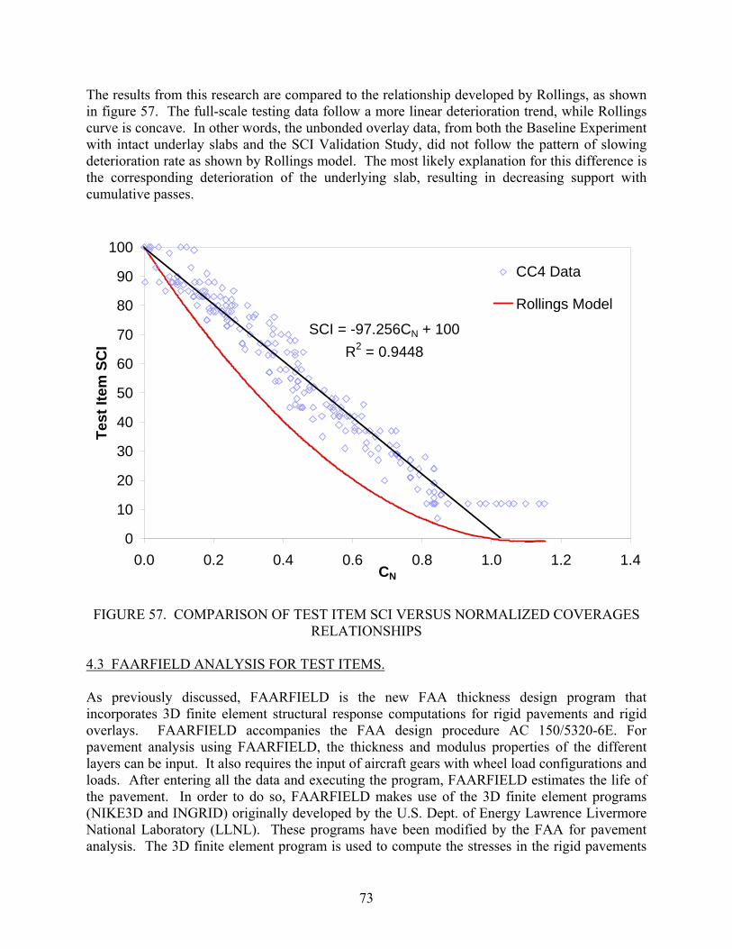
73

The results from this research are compared to the relationship developed by Rollings, as shown in figure 57. The full-scale testing data follow a more linear deterioration trend, while Rollings curve is concave. In other words, the unbonded overlay data, from both the Baseline Experiment with intact underlay slabs and the SCI Validation Study, did not follow the pattern of slowing deterioration rate as shown by Rollings model. The most likely explanation for this difference is the corresponding deterioration of the underlying slab, resulting in decreasing support with cumulative passes.

SCI = -97.256CN + 100R2 = 0.9448

0

10

20

30

40

50

60

70

80

90

100

0.0 0.2 0.4 0.6 0.8 1.0 1.2 1.4CN

Test

Item

SC

I

CC4 Data

Rollings Model

FIGURE 57. COMPARISON OF TEST ITEM SCI VERSUS NORMALIZED COVERAGES

RELATIONSHIPS 4.3 FAARFIELD ANALYSIS FOR TEST ITEMS. As previously discussed, FAARFIELD is the new FAA thickness design program that incorporates 3D finite element structural response computations for rigid pavements and rigid overlays. FAARFIELD accompanies the FAA design procedure AC 150/5320-6E. For pavement analysis using FAARFIELD, the thickness and modulus properties of the different layers can be input. It also requires the input of aircraft gears with wheel load configurations and loads. After entering all the data and executing the program, FAARFIELD estimates the life of the pavement. In order to do so, FAARFIELD makes use of the 3D finite element programs (NIKE3D and INGRID) originally developed by the U.S. Dept. of Energy Lawrence Livermore National Laboratory (LLNL). These programs have been modified by the FAA for pavement analysis. The 3D finite element program is used to compute the stresses in the rigid pavements

74

and rigid overlays. During execution, FAARFIELD computes the peak edge-loading bottom tensile stress as the basis for calculation of the estimated pavement life. The FAA personnel at the NAPTF provided a modifiable version of FAARFIELD for use in this analysis, where it provides a useful tool for considering the compounded effects of changed load level, gear configuration, concrete strength, and different levels of condition, expressed as SCI. 4.3.1 FAARFIELD Computations for Test Items. With the assistance and cooperation of FAA personnel, the FAARFIELD program was modified to allow the input of the specific input values from the accelerated testing. For example, the minimum modulus value was lowered. Also, the underlay condition was allowed to be at a lower SCI than in the standard design program. In addition, the program was modified to consider terminal values of SCI other than 80. This enables the comparison of multiple points from each test item, rather than only the passes until an SCI value of 80. The results of the FAARFIELD computations are summarized in tables 16 through 19. Results are included for a concrete modulus of rupture of 550 psi, which is the typical value of the field-cured beams. Results are also included for a concrete modulus of rupture of 700 psi, which approximates the laboratory-cured value from the design process. The estimated pavement life is very sensitive to the value of modulus of rupture, as can be seen by comparing tables 16 and 17. 4.3.2 FAARFIELD Comparisons to Observed Performance. The difference in predicted passes between modulus of rupture values of 550 psi and 700 psi to various SCI levels is quite large. The value of 550 psi for modulus of rupture represents the field-cured condition of the test slabs, while the value of 700 psi would have been a reasonable design assumption. FAARFIELD calculations were completed for both assumptions to illustrate one large difference between design assumptions and performance modeling of in situ conditions. The subsequent discussions are based upon tables 16 and 18, for a modulus of rupture of 700 psi. This simplifies the discussion, increases the number of passes to make ratios and comparisons more meaningful, and is more representative of typical design assumptions. The results would vary somewhat if the comparisons were performed for a modulus of rupture of 550 psi, but the conclusions based upon relative performance of different cross-sections and loadings would not be affected. The predicted design passes are low relative to the experimental results, as shown in table 20. From table 20, it is clear that FAARFIELD underpredicted the number of passes prior to an SCI of 80 for both the Baseline Experiment and SCI Validation Study, with the exception of Baseline Experiment data for test items N1 and S1. However, FAARFIELD is a design program, and is calibrated to include environmental effects and other factors, for design lives that extend over many years.

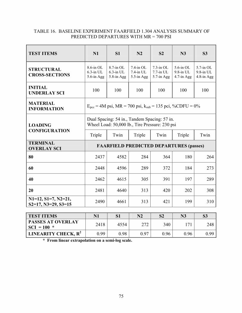
75

TABLE 16. BASELINE EXPERIMENT FAARFIELD 1.304 ANALYSIS SUMMARY OF PREDICTED DEPARTURES WITH MR = 700 PSI

TEST ITEMS

N1

S1

N2

S2

N3

S3

STRUCTURAL CROSS-SECTIONS

8.6-in OL 6.3-in UL 5.6-in Agg






INITIAL UNDERLAY SCI 100 100 100 100 100 100

MATERIAL INFORMATION Epcc = 4M psi, MR = 700 psi, ksub = 135 pci, %CDFU = 0%

Dual Spacing: 54 in., Tandem Spacing: 57 in. Wheel Load: 50,000 lb., Tire Pressure: 230 psi

LOADING CONFIGURATION

Triple Twin Triple Twin Triple Twin

TERMINAL OVERLAY SCI FAARFIELD PREDICTED DEPARTURES (passes)

80 2437 4582 284 364 180 264

60 2448 4596 289 372 184 273

40 2462 4615 305 391 197 289

20 2481 4640 313 420 202 308

N1=12, S1=7, N2=21, S2=17, N3=29, S3=15 2490 4661 313 421 199 310

TEST ITEMS N1 S1 N2 S2 N3 S3 PASSES AT OVERLAY SCI = 100 * 2418 4554 272 340 171 248

LINEARITY CHECK, R2 0.99 0.98 0.97 0.96 0.96 0.99* From linear extrapolation on a semi-log scale.

76

TABLE 17. BASELINE EXPERIMENT FAARFIELD 1.304 ANALYSIS SUMMARY OF PREDICTED DEPARTURES WITH MR = 550 PSI

TEST ITEMS

N1

S1

N2

S2

N3

S3














80 152 248 30 37 22 31

60 154 250 31 38 24 32

40 156 253 33 41 26 34

20 160 258 36 44 27 37

N1=12, S1=7, N2=21, S2=17, N3=29, S3=15 159 261 36 45 26 37


LINEARITY CHECK, R2 0.95 0.97 0.97 0.97 0.96 0.97* From linear extrapolation on a semi-log scale.

77

TABLE 18. SCI VALIDATION STUDY FAARFIELD 1.304 ANALYSIS SUMMARY OF PREDICTED DEPARTURES WITH MR = 700 PSI

TEST ITEMS

N1

S1

N2

S2

N3

S3





8.2-in.OL 7.4-in UL 5.7-in Agg









80 68 84 50 34 318 433

60 89 109 66 45 420 468

40 116 143 87 59 478 550

20 152 187 113 78 589 623*

N1=12, S1=18, N2=29, S2=66, N3=27, S3=39 169 192 100 42 570 555


LINEARITY CHECK, R2 1 1 1 1 0.98 0.97* From linear extrapolation on a semi-log scale.

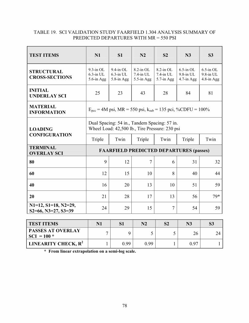
78

TABLE 19. SCI VALIDATION STUDY FAARFIELD 1.304 ANALYSIS SUMMARY OF PREDICTED DEPARTURES WITH MR = 550 PSI

TEST ITEMS

N1

S1

N2

S2

N3

S3














80 9 12 7 6 31 32

60 12 15 10 8 40 44

40 16 20 13 10 51 59

20 21 28 17 13 56 79*

N1=12, S1=18, N2=29, S2=66, N3=27, S3=39 24 29 15 7 54 59


LINEARITY CHECK, R2 1 0.99 0.99 1 0.97 1* From linear extrapolation on a semi-log scale.

79

TABLE 20. FAARFIELD DESIGN AND EXPERIMENTAL OBSERVATIONS OF CUMULATIVE PASSES TO SCI OF 80

Baseline Experiment Test Item N1 S1 N2 S2 N3 S3 FAARFIELD Design Passes to Overlay SCI=80 (MR =700 psi) 2437 4582 284 364 180 264

Accelerated Testing Passes to Overlay SCI =80 2456 3762 2456 5524 2574 3300

SCI Validation Study Test Item N1 S1 N2 S2 N3 S3 FAARFIELD Design Passes to Overlay SCI=80 (MR = 700 psi) 68 84 50 34 318 433

Accelerated Testing Passes to Overlay SCI =80 5000 15000 10000 23000 12500 24000

In order to facilitate comparison of the relative performance of the test items to the FAARFIELD designs, the number of passes to reach an overlay SCI of 80 was normalized. All values were divided by the FAARFIELD design passes to reach an SCI of 80 for the Baseline Experiment test item N2 (284 passes), for the input parameters given in table 20. The normalized values are shown in table 21. TABLE 21. NORMALIZED FAARFIELD DESIGN AND EXPERIMENT OBSERVATIONS

OF CUMULATIVE PASSES TO SCI OF 80 (PASSES/BASELINE FAARFIELD PASSES FOR N2)

Baseline Experiment Test Item N1 S1 N2 S2 N3 S3 Normalized FAARFIELD Design Passes to Overlay SCI=80 8.58 16.13 1.00 1.28 0.63 0.93

Normalized Accelerated Testing Passes to Overlay SCI =80 8.65 13.25 8.65 19.45 9.06 11.62

SCI Validation Study Test Item N1 S1 N2 S2 N3 S3 Normalized FAARFIELD Design Passes to Overlay SCI=80 0.24 0.30 0.18 0.12 1.12 1.52


80

4.3.2.1 Performance of Overlay to Underlay Thickness Ratios. The predicted performance of the three pavement structural sections is quite different from the experimental results. In order to compare the relative performance of the thickness ratios, the passes were normalized in table 22, by dividing by the passes for those for the same testing or design conditions for the ho/hu = 1.0 test items (N2 and S2). For the Baseline Experiment, with new and intact underlay slabs, FAARFIELD predicts the ho/hu = 0.6 test items (N3 and S3) to have the lowest design passes to an overlay SCI of 80, at about 60 to 70 percent of those for N2 and S2. The FAARFIELD design passes for the ho/hu = 1.5 test items (N1 and S1) are much greater by a factor of 8 to 12. However, the Baseline Experiment testing results are much different. In terms of passes to an overlay SCI of 80, all North test items performed similarly. For the South test items, the ho/hu = 1.0 test item (S2) had more passes. For the Baseline Experiment, the greatest anomaly with the thickness ratios, as compared to FAARFIELD, is that the thick-over-thin structural cross-section did not have superior performance. TABLE 22. NORMALIZED FAARFIELD DESIGN AND EXPERIMENT OBSERVATIONS

OF CUMULATIVE PASSES TO SCI OF 80 (NORTH PASSES/N2 PASSES; SOUTH PASSES/S2 PASSES)





For the SCI Validation Study, the comparisons of thickness ratios are somewhat more complicated. The thickness ratios are confounded with the underlay condition. However, as previously noted, FAARFIELD was modified to allow for the input of the low initial SCI values for the N1, S1 and N2 test items. Therefore, the relative performance as compared to FAARFIELD can still be assessed, using the ratios in Table 22. For the SCI Validation Study, FAARFIELD output yielded higher design passes to an overlay SCI of 80 for both the ho/hu = 0.6 test items (with high underlay SCI values) and the ho/hu = 1.5 test items (with low underlay SCI values), than for the ho/hu = 1.0 test items (with intermediate to low SCI values). However, the experimental results yielded much less difference between the

81

test items. The thin-over-thick test items (N3 and S3) did have the most passes to reach an overlay SCI of 80, but only by a small percentage. The ho/hu = 1.0 test items performed almost as well, despite the poorer condition of the underlay slabs. 4.3.2.2 Effect of Underlay SCI. The effect of underlay SCI is confounded with the decrease in load levels between the Baseline Experiment and the SCI Validation Study. However, the FAARFIELD program stress computations account for this load decrease. Therefore, the passes to an SCI of 80 for the SCI Validation Study can be compared relative to the FAARFIELD results. For this purpose, FAARFIELD results will be compared to FAARFIELD results, and experimental results to experimental results. This helps to minimize the effect of any input-value assumptions or approximations. The increase in FAARFIELD design passes with decreasing underlay SCI is not nearly as large as indicated by the full-scale testing. After accounting for the decreased wheel load level in the SCI Validation Study, the FAARFIELD program still produced many fewer design passes to an SCI of 80 for test items N1, S1, N2 and S2. In other words, the FAARFIELD program would have allowed fewer design passes for the test items in the SCI Validation Study with underlay SCI values of less than 50 than for the Baseline Experiment with intact underlay slabs. As shown in table 23, the FAARFIELD design passes for those test items are only from 2 to 18 percent of those for the Baseline Experiment. However, the accelerated testing experiment required from approximately 2 to 4 times as many passes to reach an overlay SCI of 80 in the SCI Validation Study for test items N1, S1, N2 and S2, as it did for the Baseline Experiment. TABLE 23. NORMALIZED FAARFIELD DESIGN AND EXPERIMENT OBSERVATIONS

OF CUMULATIVE PASSES TO SCI OF 80 (PASSES/BASELINE PASSES)





In this regard, the FAARFIELD program apparently over-corrects for the cracked slab condition. This is somewhat contradicted by analysis of the HWD data, as presented in chapter 5. Also, as

82

FAARFIELD is a design program, its calibration may be accounting for environmental effects beyond the accelerated load test conditions interacting with the underlay distress. For test items N3 and S3, the underlay slabs were less distressed, with initial SCI values of about 80. The FAARFIELD design passes to an overlay SCI of 80 were approximately 70 percent greater than those for the Baseline Experiment at the higher load level. However, the observed passes in the SCI Validation Study were from 4 to 7 times greater than those observed in the Baseline Experiment In summary, the test items in the SCI Validation Study all experienced a significantly greater ratio of passes to an overlay SCI of 80, as compared to the Baseline Experiment, than was predicted by FAARFIELD. 4.3.2.3 Effect of Gear Configuration. One experimental consideration was to examine the relative performance of the structural sections under loading from the triple dual tandem and twin dual tandem gear configurations. The wheel loads were the same for both gears, resulting in a gross weight for the triple dual tandem gear of 150 percent of the gross weight for the twin dual tandem. To simplify this consideration, given the confounding factors of underlay condition and thickness ratios, in tables 24 and 25, the results are presented in terms of ratios of passes to reach incremental SCI levels. Table 24 presents the south/north ratios from FAARFIELD, while table 25 provides the same results from the experimental observations. For the Baseline Experiment, all underlay slabs were initially in new and intact condition, so the ratios are descriptive of the relative performance. For the SCI Validation Study, the N1 and S1 underlays were in similar condition with low SCI values, and the N3 and S3 underlays both had high SCI values of approximately 80. The exception is for the N2 and S2 test items in the SCI Validation Study, for which the N2 underlay had a higher initial SCI than the S2 underlay. Examination of tables 24 and 25 indicates that for the thin-over-thick test items (ho/hu = 0.6), the experimental ratios between the passes of the twin dual tandem and the triple dual tandem corresponded well to those from FAARFIELD, and averaging approximately the difference in gross gear load. However, for the thick-over-thin test items (ho/hu = 1.5), the ratio of passes increased as the underlay deteriorated. For the SCI Validation Study, in which the N1 and S1 underlays had low initial SCI values, FAARFIELD design passes were approximately equal to the ratio between the gross gear loads. However, the experimental passes from the twin dual tandem exceeded that from the triple dual tandem by almost twice the ratio between gross gear loads. For the N2 and S2 test items, the ratio of passes from FAARFIELD was the lowest; the reasons for that have not been fully identified, and may be an artifact of slightly different thicknesses and other inputs. However, the experimental results consistently produced a very high ratio between the passes to any SCI level for S2 and N2. As has been previously noted, the exceptional durability of test item S2 resulted in the necessary cessation of testing before its overlay SCI fell

83

below 60. Post-experiment deconstruction and limited testing did not reveal any clear explanation for this performance; neither did examination of the relative strains from the instrumentation data.

TABLE 24. RATIOS OF DESIGN PASSES TO OVERLAY SCI VALUES FROM FAARFIELD 1.304 (SOUTH/NORTH)

Baseline Experiment

Overlay SCI

Section 1 Pass Ratio (S1/N1)



80 1.9 1.3 1.5 60 1.9 1.3 1.5 40 1.9 1.3 1.5 20 1.9 1.3 1.5

SCI Validation Study 80 1.6 1.2 1.4 60 1.6 1.2 1.3 40 1.6 1.2 1.3

TABLE 25. EXPERIMENTAL RATIOS OF PASSES TO OVERLAY SCI VALUES

Baseline Experiment Overlay

SCI Section 1 Pass Ratio

(S1/N1) Section 2 Pass Ratio

(S2/N2) Section 3 Pass Ratio

(S3/N3) 80 1.5 2.3 1.3 60 1.6 3.0 1.4 40 2.4 3.0 1.3 20 2.2 2.7 1.9

SCI Validation Study 80 3.2 2.4 1.9 60 2.7 3.6 1.8 40 2.9 - 1.3

4.3.2.4 Relative Performance of Overlay and Underlay Slabs. The FAARFIELD outputs summarized in tables 16 through 19 also provide one tool for assessing the relative performance of the overlay and underlay slabs. To facilitate this discussion, the FAARFIELD-predicted stresses in the overlay and underlay are shown in table 26, for the tabulated input values in tables 16 and 18. These stresses can be compared to the relative condition of the overlay and underlay after the experiments. This comparison is

84

especially convenient for the Baseline Experiment, where all underlay slabs were initially in new condition. The terminal conditions for the Baseline Experiment are summarized in table 27.

TABLE 26. SUMMARY OF FAARFIELD 1.304 STRESSES

BASELINE EXPERIMENT PREDICTED STRESSES (psi) N1 S1 N2 S2 N3 S3 OVERLAY 688 665 699 673 728 685UNDERLAY 402 383 460 453 383 398

SCI VALIDATION STUDY PREDICTED STRESSES (psi) OVERLAY 626 612 647 675 551 550UNDERLAY 70 62 166 106 349 327

TABLE 27. FINAL SCI OF THE PAVEMENT LAYERS, BASELINE EXPERIMENT

SCI Layer

N1 S1 N2 S2 N3 S3

Final Overlay Condition 12 7 21 17 29 15

Final Underlay Condition 32 39 57 33 87 93 Table 26 indicates that the underlay slabs in the thin-over-thick section would be expected to experience the lowest stresses of any of the underlay slabs in the Baseline Experiment. After removal of the overlay, the N3 and S3 underlay did have the highest SCI values, by a significant margin. Although the stress levels and ending SCI values for the underlays do not correspond exactly for the other test items, the relative difference in predicted stress levels is small. The relative performance does not seem to differ significantly from FAARFIELD in this regard. 4.3.3 Summary of Findings from FAARFIELD Comparisons. From the relative comparisons of the experimental performance to the FAARFIELD predictions, the following observations can be made:

• The FAARFIELD design program is significantly conservative in life predictions as compared to the experimental sections, when the field-cured modulus of rupture is used as an input.

• FAARFIELD “over-rated” the performance of the thick-over-thin test items.

• FAARFIELD overcompensated for the effects of underlying cracking, in terms of relative

passes to an SCI of 80.

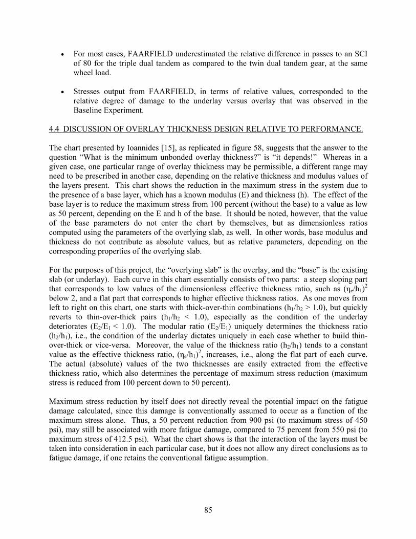
85

• For most cases, FAARFIELD underestimated the relative difference in passes to an SCI of 80 for the triple dual tandem as compared to the twin dual tandem gear, at the same wheel load.

• Stresses output from FAARFIELD, in terms of relative values, corresponded to the

relative degree of damage to the underlay versus overlay that was observed in the Baseline Experiment.

4.4 DISCUSSION OF OVERLAY THICKNESS DESIGN RELATIVE TO PERFORMANCE. The chart presented by Ioannides [15], as replicated in figure 58, suggests that the answer to the question “What is the minimum unbonded overlay thickness?” is “it depends!” Whereas in a given case, one particular range of overlay thickness may be permissible, a different range may need to be prescribed in another case, depending on the relative thickness and modulus values of the layers present. This chart shows the reduction in the maximum stress in the system due to the presence of a base layer, which has a known modulus (E) and thickness (h). The effect of the base layer is to reduce the maximum stress from 100 percent (without the base) to a value as low as 50 percent, depending on the E and h of the base. It should be noted, however, that the value of the base parameters do not enter the chart by themselves, but as dimensionless ratios computed using the parameters of the overlying slab, as well. In other words, base modulus and thickness do not contribute as absolute values, but as relative parameters, depending on the corresponding properties of the overlying slab. For the purposes of this project, the “overlying slab” is the overlay, and the “base” is the existing slab (or underlay). Each curve in this chart essentially consists of two parts: a steep sloping part that corresponds to low values of the dimensionless effective thickness ratio, such as (ηe/h1)2 below 2, and a flat part that corresponds to higher effective thickness ratios. As one moves from left to right on this chart, one starts with thick-over-thin combinations (h1/h2 > 1.0), but quickly reverts to thin-over-thick pairs (h1/h2 < 1.0), especially as the condition of the underlay deteriorates (E2/E1 < 1.0). The modular ratio (E2/E1) uniquely determines the thickness ratio (h2/h1), i.e., the condition of the underlay dictates uniquely in each case whether to build thin-over-thick or vice-versa. Moreover, the value of the thickness ratio (h2/h1) tends to a constant value as the effective thickness ratio, (ηe/h1)2, increases, i.e., along the flat part of each curve. The actual (absolute) values of the two thicknesses are easily extracted from the effective thickness ratio, which also determines the percentage of maximum stress reduction (maximum stress is reduced from 100 percent down to 50 percent). Maximum stress reduction by itself does not directly reveal the potential impact on the fatigue damage calculated, since this damage is conventionally assumed to occur as a function of the maximum stress alone. Thus, a 50 percent reduction from 900 psi (to maximum stress of 450 psi), may still be associated with more fatigue damage, compared to 75 percent from 550 psi (to maximum stress of 412.5 psi). What the chart shows is that the interaction of the layers must be taken into consideration in each particular case, but it does not allow any direct conclusions as to fatigue damage, if one retains the conventional fatigue assumption.

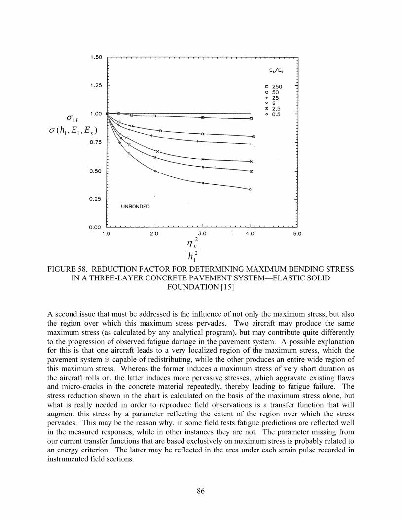
86

),,( 11

1

s

L

EEhσσ

21

2

heη

FIGURE 58. REDUCTION FACTOR FOR DETERMINING MAXIMUM BENDING STRESS IN A THREE-LAYER CONCRETE PAVEMENT SYSTEM—ELASTIC SOLID

FOUNDATION [15] A second issue that must be addressed is the influence of not only the maximum stress, but also the region over which this maximum stress pervades. Two aircraft may produce the same maximum stress (as calculated by any analytical program), but may contribute quite differently to the progression of observed fatigue damage in the pavement system. A possible explanation for this is that one aircraft leads to a very localized region of the maximum stress, which the pavement system is capable of redistributing, while the other produces an entire wide region of this maximum stress. Whereas the former induces a maximum stress of very short duration as the aircraft rolls on, the latter induces more pervasive stresses, which aggravate existing flaws and micro-cracks in the concrete material repeatedly, thereby leading to fatigue failure. The stress reduction shown in the chart is calculated on the basis of the maximum stress alone, but what is really needed in order to reproduce field observations is a transfer function that will augment this stress by a parameter reflecting the extent of the region over which the stress pervades. This may be the reason why, in some field tests fatigue predictions are reflected well in the measured responses, while in other instances they are not. The parameter missing from our current transfer functions that are based exclusively on maximum stress is probably related to an energy criterion. The latter may be reflected in the area under each strain pulse recorded in instrumented field sections.

87

5. ADDITIONAL DESIGN CONSIDERATIONS. 5.1 MATCHED VERSUS MISMATCHED JOINTS. When designing an unbonded overlay for an existing pavement, engineers are often confronted with the question of whether to deliberately match or mismatch the concrete joints. A number of studies and guides have recommended mismatching the joints to take full advantage of the load transfer provided by the support from the underlying slab [16, 17]. There have been some reservations, however, about the possible initiation of a crack in the overlay from the discontinuity below. AC 150/5320-6E states that contraction joints in unbonded overlays may be placed directly over or within one foot of existing joints [5]. However, it also provides that if a leveling course is used, the joint pattern does not have to match. The Advisory Circular also recommends a maximum slab dimension of 20 feet for unreinforced concrete. When older slabs are larger than this, a designer attempting to match joints may face a dilemma. As described in chapter 2, and illustrated in figures 1 and 2, the Baseline Experiment and SCI Validation Study were constructed with the same pattern of matched and mismatched joints. All longitudinal joints were mismatched; that is, the longitudinal joints were offset by five feet. In each test item, a mix of matched and mismatched transverse joints were constructed, resulting in at least two slabs in each test item with matched joints on both slab ends. The mismatched transverse joints were offset by 3.5 feet. In order to assess the relative performance of the matched and mismatched transverse joints, they were examined on the basis of overall performance, load transfer efficiency, and deflections. 5.1.1 Intact Slab Life. The subdivision of the test items into matched and mismatched joints results in samples too small to use test item SCI for comparison. Several measures of comparing relative condition were attempted; all gave similar results. The method discussed here used a parameter that was named “Intact Slab Life.” To identify how the passes until observation of the first crack in a slab is related to a joint that is matched or mismatched, an index named “Intact Slab Life” (ISL) was defined as the number of passes prior to the first crack in a specific slab normalized to the number of passes until the test item SCI equaled 80, defined as failure. The computed ISL values are provided in table 28 for both the north and south test items of the Baseline Experiment and the SCI Validation Study. For visual comparison, the values are plotted on bar charts in figure 59.

88

TABLE 28. CALCULATED INTACT SLAB LIFE FOR TEST ITEMS

Baseline Intact Slab Life, % SCI Validation Intact Slab Life, % Test Item Matched Mismatched Test Item Matched Mismatched

N1 (UL SCI=100) 99.0 94.1 N1

(UL SCI=25) 121.6 216.9

N2 (UL SCI=100) 106.6 86.7 N2

(UL SCI=43) 130.6 265.1

N3 (UL SCI=100) 104.5 108.3 N3

(UL SCI=84) 135.5 90.5

S1 (UL SCI=100) 140.3 166.4 S1

(UL SCI=23) 133.4 179.8

S2 (UL SCI=100) 126.2 145.7 S2

(UL SCI=26) 95.6 183.3

S3 (UL SCI=100) 162.1 106.6 S3

(UL SCI=82) 97.8 108.0

When the underlay slabs are new and intact, as in the Baseline Experiment, there is no evidence showing that slabs with matched joint and slabs with mismatched joint have different effects on the intact slab life. When the PCC underlay is damaged, as in the SCI Validation Study, which is mostly the condition for application of unbonded concrete overlay, slabs with mismatched joint have significantly longer intact life compared to those with matched joints for test items N1, S1, N2 and S2. The difference is still minimal or reversed for S3 and N3, respectively, which had the higher underlay SCI values at the beginning of the SCI Validation Study load testing. 5.1.2 Load Transfer Efficiency. Figure 60 illustrates an example comparison of the deflection load transfer efficiency, from testing after construction before subjecting to loading. As might be expected, with new tight overlay joints, there is no significant difference in the LTE values. This observation was consistent across both experiments and all test items. After the loading was initiated, the structural conditions of test items began to deteriorate and the LTE values dropped with time, as was illustrated in figures 43 and 44. To identify whether there was a difference between the deflection load transfer deterioration of matched and mismatched joints, matched and mismatched joints were plotted separately in those chapter 3 figures. In general, load transfer efficiency of matched joints tended to deteriorate faster than for mismatched joint. However, when the overlay slabs are thinner than the underlying slabs, the load transfer deterioration is less affected by joint matching.

89

020406080

100120140160180

S1 (ULSCI=100)

S2 (ULSCI=100)

S3 (ULSCI=100)

Inta

ct S

lab

Life

, %

0

50

100

150

200

250

300

N1 (UL SCI=25) N2 (UL SCI=43) N3 (UL SCI=84)

Inta

ct S

lab

Life

, %

Matched JointsMismatched Joints

020406080

100120140160180200

S1 (UL SCI=23) S2 (UL SCI=26) S3 (UL SCI=82)

Inta

ct S

lab

Life

, %

FIGURE 59. INTACT SLAB LIFE OF BASELINE EXPERIMENT (TOP) AND SCI VALIDATION STUDY (BOTTOM)

0

20

40

60

80

100

120

N1 (ULSCI=100)

N2 (ULSCI=100)

N3 (ULSCI=100)

Inta

ct S

lab

Life

, %

90

50556065707580859095

100

S1 (UL SCI=23) S2 (UL SCI=26) S3 (UL SCI=81)

Initi

al D

efle

ctio

n LT

E, %

Matched Joints Mismatched Joints

FIGURE 60. INITIAL LTE COMPARISON EXAMPLE

5.1.3 Deflections. Using the HWD data, deflection basin areas were calculated for each slab as one simple method of considering the composite structural capacity of the pavement sections over the extent of the deflection basin sensors. Deflection basins were smaller when the underlying slabs were intact (Baseline Experiment), and the values of deflection basin area decreased with increase of thickness and SCI value of the underlying slabs. The unbonded concrete overlay slabs with matched joints generally had better structural capacity, in terms of deflection basin area, than those with mismatched joint because the deflection basin values are smaller. A summary of calculated average Do (maximum deflection directly under the HWD load) is provided in table 29. Maximum deflection, normalized to a uniform load level, is another very simple way to compare structural responses, but may not capture the effect of as much underlying area as deflection basin area. The normalized D0 values increased after the underlying slabs were damaged, but there is no clear trend of difference between slabs with matched and mismatched joints.

TABLE 29. SUMMARY OF CALCULATED AVERAGE D0

D0 Normalized to 37250-lb Load Level (mils) Test Items Matched-Intact Matched-Damaged N1 and S1 11.5 mils 12.2 (SCI = 25) 10.7 (SCI = 23) N2 and S2 8.5 mils 10.5 (SCI = 43) 10.4 (SCI =26) N3 and S3 9.5 mils 10.8 (SCI = 86) 11.4 (SCI = 81)

Test Items Mismatched-Intact Mismatched-Damaged N1 and S1 9.9 mils 12 (SCI = 25) 11.6 (SCI = 23) N2 and S2 9.3 mils 10.2 (SCI = 43) 10.1 (SCI = 26) N3 and S3 11.1 mils 11.1 (SCI = 86) 10.4 (SCI = 81)

91

5.1.4 Summary of Observed Effects of Matched and Mismatched Joints. Although matched and mismatched transverse joints exhibited slightly different mechanical behavior for the unbonded overlay, the passes prior to the first crack or to failure were affected more by other structural parameters such as thickness and SCI. In addition, no direct crack propagation from underlying joints was observed during deconstruction of either the Baseline Experiment or SCI Validation Study overlays. Based upon the findings of this project, factors other than joint matching should control slab size and joint layout. There was some evidence that better overall performance was obtained with the mismatched transverse joints. 5.2 RELATIONSHIP BETWEEN UNDERLYING PAVEMENT EFFECTIVE MODULUS AND SCI – THE CRACKED SLAB MODEL. To account for the reduced support when an unbonded overlay is placed over a distressed existing concrete pavement, Rollings developed a relationship between modulus ratio and the SCI of the existing pavement [2]. This relationship is key to the unbonded overlay design assumptions within FAARFIELD, and is used for other analyses as well. The unbonded overlay experiments at the NAPTF were designed to examine this relationship with techniques not typically available in the field. This section provides a summary of some of the analysis that was undertaken in that regard, and the key findings that resulted. 5.2.1 Rollings Model Background. For the development of the relationship, slabs were broken and tested with a falling weight deflectometer. The procedure followed at the Waterways Experiment Station (WES) is summarized here so the similarities and differences in procedures and assumptions to the current experiments are clear. The process was as follows [2]: 1. Slabs were placed directly on top of the native loess subgrade (classified as CL by USCS)

and were slightly reinforced at mid-depth. 2. Cracks were introduced by dropping a headache ball at selected locations to control the

development of cracks. 3. Deflection basins were obtained by utilizing a falling weight deflectometer (FWD), model

Dynatest 8000, at each crack stage during the experiment. The consistency of readings from each drop (total four drops for each location) was analyzed and the most consistent one, excluding the first reading was used for backcalculation with BISDEF.

4. In BISDEF, a backcalculation program based on elastic layer theory using the well-known

program BISAR, an artificial rock bed, with 1 million psi elastic modulus and 0.5 Poisson’s ratio, was assumed at a depth of 20 ft to obtain accurate surface deflection predictions. The

92

Poisson’s ratio for subgrade was assumed to be 0.4, and the modulus was fixed at 10 thousand psi. The Poisson’s ratio for concrete was assumed to be 0.15.

5. SCI was calculated based on an assumption that the appearance of a crack type in a slab

represented that 50 percent of slabs within a test item would exhibit that crack type and severity.

6. For backcalculation, the effective modulus of concrete was taken as that which matched the

deflection under the center of the plate with BISAR. This was done to prevent false readings due to the crack discontinuities.

7. For each slab, deflection basins were obtained at three locations. Backcalculation of three

deflection basins was done and compared to determine which one was reasonable to be used as baseline for further analysis.

Based upon those test results, a relationship between SCI and E-Ratio was found with linear regression methods, and is provided here as equation 4. E-Ratio is the ratio between the effective modulus in the cracked condition, and the original modulus of the slab. Equation 4 is used to characterize both overlay and underlay slabs elastic moduli at specific structural conditions of an unbonded concrete overlay system, and is defined as the “Cracked Slab Model.”

2)00584.0(0064.002.0 SCISCIRatioE ×+×+=− (3) r2 = 0.95 N = 24

The cracked slab model represents an extremely significant advance for mechanistic-empirical design of unbonded concrete overlays. However, the data used for the development of the model was necessarily limited, partly by being restricted to only 24 data points. Some specific additional limitations include:

• The WES slab tests consisted of six single concrete slabs placed directly on the subgrade, while unbonded concrete overlays include multiple layers within the pavement system.

• SCI was calculated based on a single slab and the crack density of each type of crack was

always fixed at 50 percent.

• Effective modulus was backcalculated based on only the deflection under the center of the plate. This was a necessary assumption because of the surface discontinuities.

5.2.2 Examination of the Single Slab SCI Calculation using the Unbonded Overlay Data. Based on the information from distress surveys conducted regularly during the Baseline Experiment and SCI Validation Study, and upon the corresponding HWD data, the relationship between SCI and corresponding effective concrete modulus ratio can be verified. This data has its own limitations—it is indoors, there is only one subgrade type, and the cracking pattern was

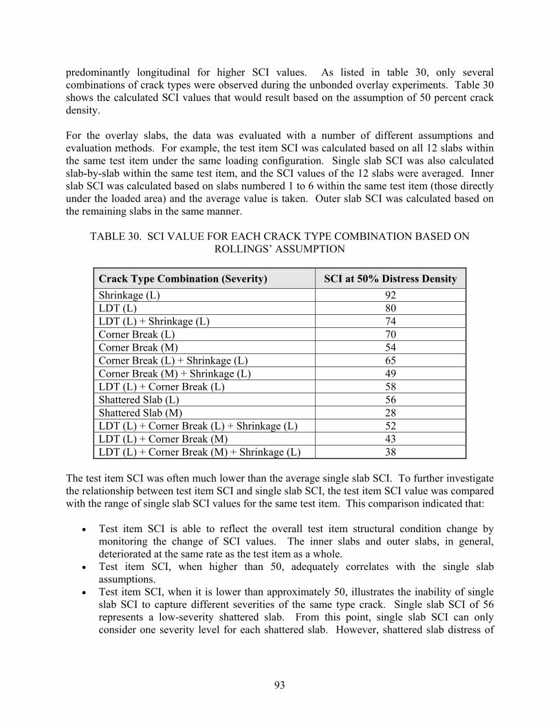
93

predominantly longitudinal for higher SCI values. As listed in table 30, only several combinations of crack types were observed during the unbonded overlay experiments. Table 30 shows the calculated SCI values that would result based on the assumption of 50 percent crack density. For the overlay slabs, the data was evaluated with a number of different assumptions and evaluation methods. For example, the test item SCI was calculated based on all 12 slabs within the same test item under the same loading configuration. Single slab SCI was also calculated slab-by-slab within the same test item, and the SCI values of the 12 slabs were averaged. Inner slab SCI was calculated based on slabs numbered 1 to 6 within the same test item (those directly under the loaded area) and the average value is taken. Outer slab SCI was calculated based on the remaining slabs in the same manner.

TABLE 30. SCI VALUE FOR EACH CRACK TYPE COMBINATION BASED ON

ROLLINGS’ ASSUMPTION

Crack Type Combination (Severity) SCI at 50% Distress Density Shrinkage (L) 92 LDT (L) 80 LDT (L) + Shrinkage (L) 74 Corner Break (L) 70 Corner Break (M) 54 Corner Break (L) + Shrinkage (L) 65 Corner Break (M) + Shrinkage (L) 49 LDT (L) + Corner Break (L) 58 Shattered Slab (L) 56 Shattered Slab (M) 28 LDT (L) + Corner Break (L) + Shrinkage (L) 52 LDT (L) + Corner Break (M) 43 LDT (L) + Corner Break (M) + Shrinkage (L) 38

The test item SCI was often much lower than the average single slab SCI. To further investigate the relationship between test item SCI and single slab SCI, the test item SCI value was compared with the range of single slab SCI values for the same test item. This comparison indicated that:

• Test item SCI is able to reflect the overall test item structural condition change by monitoring the change of SCI values. The inner slabs and outer slabs, in general, deteriorated at the same rate as the test item as a whole.

• Test item SCI, when higher than 50, adequately correlates with the single slab assumptions.

• Test item SCI, when it is lower than approximately 50, illustrates the inability of single slab SCI to capture different severities of the same type crack. Single slab SCI of 56 represents a low-severity shattered slab. From this point, single slab SCI can only consider one severity level for each shattered slab. However, shattered slab distress of

94

different severities might be exhibited within the same test item, which will further lower the SCI value for the test item.

In summary, there is sometimes a significant difference between test item SCI and single slab SCI. This demonstrates one advantage in having 12-slab test items to use for verification. 5.2.3 Cracked Slab Model Verification. Verification of the cracked slab model was investigated with the overlay slab data. Alternate methods of characterizing the condition, including an array of crack density approaches, were also conducted. The procedures and results are summarized in the research report. However, in this report, the results from utilizing a set of data unique to this experiment are presented. From the construction stage of the Baseline Experiment, through the deconstruction of the SCI Validation Study, the test item underlay slabs were exposed for detailed inspection at four condition levels. For each of those condition levels, HWD testing was performed on the overlay slabs either after placement or before removal. Therefore, the underlay modulus values could be backcalculated for the in-place conditions with an unbonded overlay providing confinement. Those backcalculated values could be compared to the known corresponding cracking patterns. To verify the cracked model, concrete underlay average E-Ratio at different SCI conditions was used. A summary of the data is provided in table 31. The details of the backcalculation procedures and assumptions were presented in chapter 3, as were the distress survey and SCI calculation techniques. The visual condition of the concrete underlays can only be known at the beginning of each experiment before overlay placement, and at the end of each experiment after the removal of overlay. As a result, only 24 points are available as listed in table 31. For this analysis, the average backcalculated modulus for the underlay below the loaded area was utilized.

TABLE 31. UNDERLAY TEST ITEM SCI AND BAKFAA RESULTS

Baseline SCI Validation

Initial Final Initial Final

Test Item SCI

Average Inner-Slab

BAKFAA Modulus

(psi) SCI

Average Inner-Slab

BAKFAA Modulus

(psi) Test Item SCI

Average Inner-Slab

BAKFAA Modulus

(psi) SCI

Average Inner-Slab

BAKFAA Modulus

(psi) N1 100 9.13E+06 32 3.42E+06 N1 25 3.07E+06 3 1.32E+06 N2 100 7.82E+06 57 3.94E+06 N2 43 4.82E+06 17 1.86E+06 N3 100 9.03E+06 87 4.66E+06 N3 84 4.95E+06 26 2.44E+06 S1 100 7.69E+06 39 5.44E+06 S1 23 2.07E+06 8 1.62E+06 S2 100 1.00E+07 33 3.96E+06 S2 28 2.88E+06 9 2.35E+06 S3 100 7.66E+06 93 6.27E+06 S3 81 4.92E+06 23 2.72E+06

95

Figure 61 illustrates Rollings’ cracked slab model as a solid line, with the data from table 31 shown as points. The BAKFAA average inner slab modulus of 7/25/2006 was used as the initial modulus (E0) and start of the Baseline Experiment. The BAKFAA average inner slab modulus values for the end of Baseline, the start of SCI Validation and the end of SCI Validation were obtained from the HWD testing conducted on 11/7/2006, 10/22/2007 and 5/29/2008, respectively. The modulus of each test item from these three dates was normalized by dividing by its initial modulus and was compared to the corresponding test item SCI value.

0.00

0.20

0.40

0.60

0.80

1.00

0 20 40 60 80 100Underlay Test Item SCI

BA

KFA

A In

ner S

lab

E-R

atio

.

FIGURE 61. UNDERLAY TEST ITEM SCI VERSUS E-RATIO FOR ROLLINGS MODEL (SOLID LINE) AND THE EXPERIMENTAL UNDERLAY DATA (POINTS)

This plot of underlay inner slab E-ratio versus underlay test item SCI shows a reasonable degree of agreement with Rollings’ model, although there are some deviations. For higher levels of SCI, the experimental data fell below the line, indicating lower modulus values than predicted. For lower values of SCI, the experimental data fell above the line, indicating higher modulus values than predicted. One explanation for the higher values at low SCIs may be the confined condition under the overlay, as opposed to the exposed slabs in the WES experiment. The

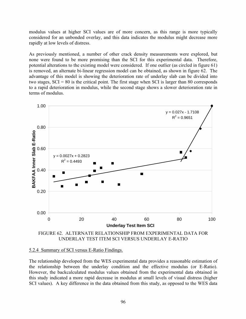
96

modulus values at higher SCI values are of more concern, as this range is more typically considered for an unbonded overlay, and this data indicates the modulus might decrease more rapidly at low levels of distress. As previously mentioned, a number of other crack density measurements were explored, but none were found to be more promising than the SCI for this experimental data. Therefore, potential alterations to the existing model were considered. If one outlier (as circled in figure 61) is removed, an alternate bi-linear regression model can be obtained, as shown in figure 62. The advantage of this model is showing the deterioration rate of underlay slab can be divided into two stages, SCI = 80 is the critical point. The first stage when SCI is larger than 80 corresponds to a rapid deterioration in modulus, while the second stage shows a slower deterioration rate in terms of modulus.

y = 0.027x - 1.7108R2 = 0.9651

y = 0.0027x + 0.2823R2 = 0.4493

0.00

0.20

0.40

0.60

0.80

1.00

0 20 40 60 80 100Underlay Test Item SCI

BA

KFA

A In

ner S

lab

E-R

atio

FIGURE 62. ALTERNATE RELATIONSHIP FROM EXPERIMENTAL DATA FOR

UNDERLAY TEST ITEM SCI VERSUS UNDERLAY E-RATIO

5.2.4 Summary of SCI versus E-Ratio Findings. The relationship developed from the WES experimental data provides a reasonable estimation of the relationship between the underlay condition and the effective modulus (or E-Ratio). However, the backcalculated modulus values obtained from the experimental data obtained in this study indicated a more rapid decrease in modulus at small levels of visual distress (higher SCI values). A key difference in the data obtained from this study, as opposed to the WES data

97

is that these slabs are in the “underlay” position, confined as an existing pavement would be after placement of an unbonded overlay. However, these slabs were also confined during the development of that initial visible cracking. This may have slowed progression to a visible level, but still lowered the modulus. One other observation is that while this model indicates an under-estimation of the impact of underlay deterioration on stiffness, the FAARFIELD analysis described in chapter 4 indicated that FAARFIELD over-estimated the detrimental effects at various SCI levels. Additional analysis of the data collected during this experiment is recommended to further evaluate the interaction between overlay deterioration, underlay deterioration and effective modulus for use in mechanistic design. 6. SUMMARY AND CONCLUSIONS. 6.1 OVERVIEW OF PROJECT INFORMATION. The IPRF unbonded overlay experiments at the NAPTF encompassed two interfaced consecutive experiments. In the Baseline Experiment, unbonded overlays were constructed over new intact underlying pavement of varying thicknesses. After loading to failure, the overlay was removed. During the SCI Validation Study, new unbonded overlays were placed over the distressed underlay slabs, and were again loaded to failure. While some analysis and observations were possible from the Baseline Experiment alone, the greatest trove of information to be developed comes from looking at the two experiments together. This report has provided a summary overview of both experiments, and focused on the integrated data analysis, that has resulted in key findings with implications for unbonded overlay design. Further documentation of all stages of the experimental testing and resulting data are available in the project research reports. Much instrumentation data remains to be fully processed and analyzed, and that work is ongoing after these projects are complete. The project data will be available to the public upon request. 6.2 SUMMARY OF FINDINGS AND CONCLUSIONS PRESENTED IN THIS REPORT. In chapter 2, the construction of the test items, loading with the test vehicle, data collection, and subsequent deconstruction were described. Some key notations from chapter 2 were:

• Despite attempts to increase the flexural strength for the SCI Validation Study, both experiments had field-cured modulus of rupture values of approximately 550 psi.

• During removal of the overlay, visual observations indicated that cracks did not

propagate directly from underlying discontinuities, through the asphalt interlayer, and into the overlay slabs. This is an empirical reinforcement that the approximately one-inch asphalt concrete served as an effective interlayer.

98

• The post-loading modulus of subgrade reaction values, from plate load tests, were lower than the preconstruction values for all test items.

• After load-testing, vane shear test results showed an increase in subgrade stiffness at a 6-

inch depth, but a decrease at the surface. This may be related to a moisture gradient that developed due to the watering and loading interactions, but the causes were not further investigated by the project team.

Chapter 3 provided direct results of the experiments, in the form of distress maps, SCI calculations, backcalculation of moduli from HWD testing, and processing of instrumentation responses. Important observations included:

• During the Baseline Experiment, with stiff intact slabs underlying the overlay, the initial cracks were longitudinal, and longitudinal cracking continued to predominate as the overlay deteriorated. The first cracks to be observed were confirmed by coring to be top-down cracks just outside the loaded area, followed quickly by bottom-up cracks underneath the load.

• During the SCI Validation Study, with damaged slabs underlying the overlay, the initial

cracks were again longitudinal. However, a variety of crack manifestations progressed. The cracks were not directly propagated from underlying cracks, but the greatest distress concentrations were in the slabs which had more distressed underlay slabs below.

• The continued deterioration of the underlay slabs, which remained in place throughout

both experiments, could be seen in the progressive decrease of backcalculated moduli.

• After placement of the new overlay, the backcalculated stiffness for the upper layer was fully recovered, as anticipated. However, some of the underlying layers also exhibited an apparent, and temporary, stiffened effect.

• The load transfer efficiency at mismatched joints deteriorated less as compared to the

load transfer efficiency at matched joints within the same test item.

• For responses normalized to the same wheel load, the soil pressure cells in the SCI Validation Study experienced significantly greater responses than those in the Baseline Experiment.

• The ratio in magnitude of peak strain produced by the triple dual tandem and twin dual

tandem gears is not inversely proportional to the number of passes until failure. The ratio of passes to achieve a given SCI is greater than can be explained only by the peak magnitude of the measured strains.

• For all ratios of overlay to underlay thickness, the peak strains from instrumentation were

larger in the overlay than in the underlay. This corresponds to the observed relative distress progression.

99

In chapter 4, the heart of the motivation for the unbonded overlay experiments was examined. Do the current design models reasonably predict the performance of the unbonded overlays, with regard to passes to failure, shape of deterioration curves and rate of deterioration, thickness ratios, underlay condition and gear configuration? Findings that were discussed in chapter 4 included:

• The South test items (loaded with the twin dual tandem) consistently required more passes to achieve a given SCI level than the North test items (loaded with the triple dual tandem) at the same wheel load. This reinforces the knowledge that gross aircraft weight is one of the most important factors in airfield pavement performance.

• The thin overlay over thick underlay cross section performed better than the researchers

had anticipated. While the overlay deteriorated at a rate similar to that of the other test items, the underlay slabs had only minor distress at the end of testing.

• The unbonded overlay data, consolidated from both experiments, did not follow the

pattern of slowing deterioration rate as shown by the Rollings relationship between CN and SCI. The testing data followed an almost linear deterioration trend. The most likely explanation for this difference is the corresponding deterioration of the underlying slabs, resulting in decreasing support with increased cumulative passes.

Regarding the relative performance predictions made by the FAARFIELD design program, the following observations were made in chapter 4:

• The FAARFIELD design program is significantly conservative in life predictions as compared to the experimental sections, when the field-cured modulus of rupture is used as an input.

• FAARFIELD “over-rated” the performance of the thick-over-thin test items.

• FAARFIELD overcompensated for the effects of underlying cracking, in terms of relative

passes to an SCI of 80.

• For most cases, FAARFIELD underestimated the relative difference in passes to an SCI of 80 for the triple dual tandem as compared to the twin dual tandem gear, at the same wheel load.

• Stress estimations from FAARFIELD, in terms of relative values, corresponded to the

relative degree of damage to the underlay versus overlay that was observed in the Baseline Experiment.

Chapter 4 closed with a discussion of overlay thickness ratios relative to performance. A need has been expressed for guidance as to what thickness ratios would perform the best. With the assistance of Dr. Ioannides’ past research [15], the definitive answer was formulated to be “it depends!” However, some assistance is provided with the illustration in figure 58, which shows the stress reduction in an unbonded overlay configuration changes as thickness ratio and modular

100

ratio vary Additionally, the discussion extended to the potential need to examine other features of the pavement strain response, other than maximum strain. Chapter 5 began with a comparison of the performance of matched and mismatched joints. All longitudinal joints were offset in both experiments, so only the relative effect of matched and mismatched transverse joints could be examined. Based upon the observations in this project, and upon the current Advisory Circular, it is recommended that factors other than joint matching should control slab size and joint layout. There was some evidence that better overall performance was obtained with the mismatched transverse joints. Finally, also in chapter 5, the relationship between underlying pavement effective modulus (or E-Ratio) and the Structural Condition Index (SCI) was examined. While the current cracked slab model was found to provide a reasonable estimation of the relationship [2], the backcalculated modulus values obtained in this study indicated a more rapid decrease in modulus at small levels of visual distress (higher SCI values). A bi-linear regression model was presented, which more closely fits the experimental data. While this seems to indicate an under-estimation of the impact of the underlay deterioration on stiffness, the FAARFIELD analysis indicated that, overall, FAARFIELD over-estimated the detrimental effects at various SCI levels. It is recommended that this topic be a focus of additional study, including further incorporation of the instrumentation data. 6.3 FINAL COMMENTS. From the results of the full-scale testing of unbonded overlays at the NAPTF, one significant observation is that the unbonded overlay rehabilitation strategy can be used successfully when the existing pavement is in a broad range of existing distress levels. The South 2 test item in the SCI Validation Study had an initial SCI value of below 30, and provided excellent performance in terms of overlay test item SCI. The durable performance was probably aided by the consistent indoor environment, but the relative passes to incremental SCI levels far exceeded what was anticipated. The results of the experiments may have significant implications for airfield pavement management and programming decisions, as well. The anticipated number of passes to progress between incremental levels of SCI will vary with design conditions. However, the linear progression of SCI decline with cumulative passes/coverages, for the normalized plot of CN and SCI, indicates that the rate of deterioration, after initial crack progression, may be higher for an unbonded overlay and perhaps for other multi-layer composite pavements designed to similar stress levels. If the stress levels in underlying layers are high enough to induce continued damage, then the support for the overlay will decline with coverages.

101

7. REFERENCES. 1. Khazanovich, L., Improved Concrete Overlay Design Parameters for Airfield Pavements

Report, DOT/FAA-01-G-002-2, published by the Innovative Pavement Research Foundation for the Aviation Administration, Washington, D.C., 2001.

2. Rollings, R.S., Design of Overlays for Rigid Airport Pavements, Report No. DOT/FAA/PM-

87/19, Federal Aviation Administration, Washington, D.C., 1988. 3. Brill, D.R., Development of Advanced Computational Models for Airport Pavement Design,

DOT/FAA/AR-97/47, Federal Aviation Administration, Washington, D.C., 1998. 4. Brill, D.R., I. Kawa, and L. Ricalde, “Comparative Study of Rigid Pavement Thickness

Designs Using FAARFIELD, 2008 FAA Working Group Meeting, Atlantic City, New Jersey, 2008.

5. Federal Aviation Administration, Airport Pavement Design and Evaluation, Advisory

Circular AC 150/5320-6E, FAA, Washington, D.C., 2009. 6. Hayhoe, G.H., “Traffic Testing Results from the FAA’s National Airport Pavement Test

Facility,” Proceedings of the 2nd International Conference on Accelerated Pavement Testing, University of Minnesota, Minneapolis, Minnesota, 2004.

7. Daiutolo, “Control of Slab Curling in Rigid Pavements at the FAA National Airport

Pavement Test Facility,” Proceedings of the 3rd International Conference on Accelerated Pavement Testing, Oct. 1-3, Madrid, Spain, 2008.

8. American Society for Testing and Materials, Standard Test Method for Airport Pavement

Condition Index Surveys, Designation D 5340-03, ASTM International, West Conshohocken, Pennsylvania, USA, 2003.

9. Garg, Navneet, E. Guo and R. McQueen, Operational Life of Airport Pavements, Technical

Report No. DOT/FAA/AR-04/46, Federal Aviation Administration, Office of Aviation Research, 2004.

10. Evangelista, Jr., F.and J.R. Roesler, Top Down Cracking Predictions for Airfield Rigid

Pavements, Transportation Research Board, Issue No. 2095, 2009. 11. Brill, D.R., G.F. Hayhoe, and L. Ricalde, “Analysis of CC2 Rigid Pavement Test Data from

the FAA’s National Pavement Test Facility,” Proceedings of the 7th International Conference on the Bearing Capacity of Roads, Railways and Airfields, Trondheim, Norway, 2005.

12. Zollinger, D.G., D. Ye, and D.A. Morian, Characterization and Analysis of Early Age

Concrete Pavement Behavior at the National Airport Pavement Test Facility (NAPTF), Texas Transportation Institute, College Station, Texas, August 2007.

102

13. Stoffels, S., D. Morian, A. Ioannides, S. Wu, S. Sadasivam, L. Yeh and H. Yin, Improved Overlay Design Parameters for Concrete Airfield Pavements, Baseline Experiment Final Report, Innovative Pavement Research Foundation (IPRF) Project FAA-01-G-002-04-02, 2008.

14. Stoffels, S., D. Morian, A. Ioannides, L. Yeh, J. Reiter and S. Wu, Improved Overlay Design

Parameters for Concrete Airfield Pavements—SCI Validation Study Research Report, Innovative Pavement Research Foundation (IPRF) Project FAA-01-G-002-06-03, 2010.

15. Ioannides, A.M., L. Khazanovich, and J.L. Becque, “Structural Evaluation of Base Layers in

Concrete Pavement Systems,” Transportation Research Record No. 1370, Transportation Research Board, National Research Council, Washington, D.C., 1992.

16. Smith, K.D., H.T. Yu, and D.G. Peshkin, “Portland Cement Concrete Overlays: State of the

Technology Synthesis,” Federal Highway Administration, Washington, D.C., 2002. 17. National Concrete Pavement Technology Center, Guide to Concrete Overlays, 2nd Edition,

Ames, Iowa, 2008.

an iprf research report innovative pavement research … report 06-3.pdf · ·...

Documents