an investigation on pvdf piezoelectric … investigation on pvdf piezoelectric elements and linear...

Master’s DissertationEngineering

Acoustics

ALI ALKHUDRI Report TV

BA-5053

ALI A

LKH

UD

RI AN

INV

ESTIGA

TION

ON

PVD

F PIEZOELEC

TRIC

ELEMEN

TS AN

D LIN

EAR

AR

RA

Y TR

AN

SDU

CER

S

AN INVESTIGATION ON PVDFPIEZOELECTRIC ELEMENTS ANDLINEAR ARRAY TRANSDUCERS

TVBA-5053HO.indd 1TVBA-5053HO.indd 1 2017-06-22 18:39:572017-06-22 18:39:57

DEPARTMENT OF CONSTRUCTION SCIENCES

DIVISION OF ENGINEERING ACOUSTICS

ISRN LUTVDG/TVBA--17/5053--SE (1-74) | ISSN 0281-8477

MASTER’S DISSERTATION

Supervisors: DELPHINE BARD, Assoc. Prof., Div. of Engineering Acoustics, LTH, Lundand STEFANOS ATHANASOPOULOS, Ph.D. Student, Div. of Solid Mechanics, LTH, Lund.

Examiner: Professor ERIK SERRANO, Div. of Structural Mechanics, LTH, Lund.

Cover image is reproduced with kind permission fromNDT Resource Center and Center for NDE, Iowa State University, USA.

Copyright © 2017 by Division of Engineering Acoustics,Faculty of Engineering LTH, Lund University, Sweden.

Printed by Media-Tryck LU, Lund, Sweden, June 2017 (Pl).

For information, address:Division of Engineering Acoustics,

Faculty of Engineering LTH, Lund University, Box 118, SE-221 00 Lund, Sweden.

Homepage: www.akustik.lth.se

ALI ALKHUDRI

AN INVESTIGATION ON PVDFPIEZOELECTRIC ELEMENTS AND

LINEAR ARRAY TRANSDUCERS

__________________________________________________________________________________

Abstract __________________________________________________________________________________

Ultrasonic waves are widely used in different application e.g. for sonar scanning in water and

fetal imaging. Furthermore it is used for doing measurements on different materials to

determine the thickness of the material or the velocity of sound inside it. The ultrasonic

waves are produced and detected by using piezoelectric elements based on e.g.

Polyvinylidene fluoride (PVDF)-film or Lead Zirconate Titanate (PZT)-elements. In this

thesis project the aim has been to do measurements on different materials and then develop a

linear array transducer based on the use of PVDF-films. Three different methods have been

studied to do the measurements on different materials. The first method has been to use a

commercial product (ultrasonic (US) key and software from Lecoeur), the second method has

been to use the same US-key but in combination with MATLAB. The US-key is an ultrasonic

device which is connected to ultrasonic transducer(s) to emit and detect ultrasonic waves.

The software was used for displaying plots from the measurements. Finally, the third method

involved the use of a generator and an oscilloscope. It has been found that the first and

second methods did not work properly to make the linear array transducer because the US-

key produced a noise artifact during measurements. The linear array transducer was made by

using two industrial ultrasonic transducers of 1-MHz which were connected to the generator

and three PVDF-films used as receivers and connected to the oscilloscope. The linear array

transducer was built up to use it for examining a specific material-aluminum. It was found

that aluminum is the best material to be used to do the ultrasonic testing because of its low

attenuation of the ultrasonic waves.

Keywords:

Ultrasonic Transducer, Piezoelectric Element, PVDF, Frequency, Ultrasound Wave

Penetration, PZT, Acoustic Impedance, raw data, linear array transducer.

Sammanfattning __________________________________________________________________________________

Ultraljudsvågor används i många olika tillämpningar, t.ex. som sonar i vatten och för

fosterdiagnostik. De kan också användas för att göra mätningar på olika material för att

bestämma materialets tjocklek eller ljudets hastighet i materialet. Ultraljudsvågorna

produceras och detekteras med hjälp av piezoelektriska element, t.ex. polyvinylidenflourid

(PVDF)-film eller så kallade PZT-element (bly-zirconium-titan). I detta projekt har målet

varit att göra mätningar på olika material och sedan utveckla en omvandlare av PVDF-film.

Tre olika metoder har studerats för att göra mätningarna på olika material. Första metoden

har varit att använda en kommersiell ultraljudsutrustning (”US-key” och programvara från

Lecoeur), den andra metoden har varit att använda samma hårdvara (”US-key”) i

kombination med MATLAB. Hårdvaran är en ultraljudsenhet som ansluts till en eller två

ultraljudsgivare för att producera och detektera ultraljudsvågor. Lecoeur-programvaran

används för att plotta mätvärdena. Slutligen har en tredje metod provats genom att använda

en generator och ett oscilloskop. Det har visat sig att den första och andra metoden inte

fungerade bra för att bygga omvandlaren eftersom den kommersiella hårdvaran skapade

störningar när mätningarna gjordes. Omvandlaren har därför byggts genom att använda två 1-

MHz ultraljudsgivare som har anslutits till en generator och tre PVDF-filmer som mottagare

som har anslutits till ett oscilloskop. Omvandlaren har sedan använts för att undersöka ett

specifikt material - aluminium. Aluminium har en låg dämpningskoefficient som gör att

ultraljudsvågorna inte dämpas för mycket.

__________________________________________________________________________________

Acknowledgments __________________________________________________________________________________

This master thesis has been carried out at Lund University, Sweden. I want to give many

thanks to Stefanos Athanasopoulos and to my supervisor Delphine Bard for their guidance

and support in the making of this thesis work.

I also want to thank my family for their support.

Lund, April 19, 2017

Ali Alkhudri

___________________________________________________________________________

Table of Contents

1 Introduction ............................................................................................................................. 1

Background ........................................................................................................................ 1

Thesis goal ......................................................................................................................... 3

Report outline .................................................................................................................... 4

2 Theory ..................................................................................................................................... 5

Piezoelectric Phenomenon ................................................................................................. 5

Generation and Detection of Ultrasonic Waves by Piezoelectric Elements ...................... 6

Speed and Wavelength ...................................................................................................... 7

Propagation of Ultrasonic Waves ..................................................................................... 8

Basic Design of an Ultrasonic Transducer ...................................................................... 13

PZT-element Compared to PVDF-film ........................................................................... 16

Frequency Response of Piezoelectric Elements .............................................................. 17

Circular and Square PVDF-film ...................................................................................... 17

Ultrasound Couplant ........................................................................................................ 18

3 Tools ..................................................................................................................................... 20

Tools from Lecoeur Electrique Company ........................................................................ 20

Linear Array Transducer by Using Two US-keys and an Interface Module ............ 21

Linear Array Transducer by Using a generator and an oscilloscope ............................... 22

4 Measurements ....................................................................................................................... 23

Measurements by US-key with Lecoeur software ........................................................... 23

Measurements by US-key with MATLAB code ............................................................. 27

Measurements by Generator and Oscilloscope ............................................................... 29

5 Results and Discussion ......................................................................................................... 31

6 Conclusions ........................................................................................................................... 37

Future work ...................................................................................................................... 38

7 References ............................................................................................................................ 39

Appendix I

Appendix II

___________________________________________________________________________

List of figures ___________________________________________________________________________

The design of an industrial ultrasonic transducer with PZT-plate [9] ....................................... 2

The design of an ultrasonic transducer with PVDF-film .......................................................... 2

Representation of the piezoelectric material [14] ...................................................................... 5

The vibration of the piezoelectric element in two different cases [11]...................................... 6

Attenuation in different thicknesses of a bright drawn steel sample and an aluminum sample.

.................................................................................................................................................... 9

Attenuation in different thicknesseses of a rock sample and a marble sample ........................ 10

Attenuation with different frequencies in aluminum and bright drawn steel samples ........... 12

Attenuation with different frequencies in rock and marble samples ...................................... 12

Two beam spread of ultrasound waves for two transducers with the same diameter ............. 13

Beam spread of ultrasonic waves from an ultrasonic transducer [16] ..................................... 13

Beam spread angle of the transmitted ultrasound waves ......................................................... 14

The relation between resonance frequency and thickness of the PVDF piezoelectric

element. .................................................................................................................................... 15

The backing layer and matching layer of an ultrasound transducer ........................................ 16

Illustration of circular and square PVDF-film ......................................................................... 17

The propagation of ultrasound waves in an aluminum sample................................................ 19

The connection of the US-key to the computer and the ultrasound transducer (probe) [28] ... 20

The interface module for connecting the PVDF-film to the US-key [29] ............................... 21

The layout of the linear array transducer with one emitter and two receivers with US-keys .. 21

The layout of the linear array transducer with two emitters and three receivers

by using generator and oscilloscope ........................................................................................ 22

The noise artifact from the US-key by using Lecoeur software .............................................. 27

The noise artifact from the US-key by using MATLAB code................................................. 29

The square PVDF of length 1 cm to and circular PVDF of diameter 1 cm ............................. 31

The square PVDF of length 1.25 cm to and circular PVDF of diameter 1.25 cm ................... 32

The square PVDF of length 1.5 cm to and circular PVDF of diameter 1.5 cm ....................... 32

Difference between using PVDF-film as emitter and as receiver ............................................ 33

The recorded raw data by oscilloscope from the three PVDF-films ...................................... 34

The recorded signal by first oscilloscope channel with its amplitude spectrum

and power spectral density ....................................................................................................... 35

The recorded signal by second oscilloscope channel with its amplitude spectrum


The recorded signal by third oscilloscope channel with its amplitude spectrum


___________________________________________________________________________

List of tables ___________________________________________________________________________

Ultrasound frequencies in sonar, pregnancy scan and animal communication [1, 7, 8] ........... 1

Names of Transducers and Piezoelectric Materials

which were used to do measuremens ........................................................................................ 3

Different speeds of the ultrasound waves in different materials [23] ........................................ 7

Attenuation coefficients for different materials at 1-MHz frequency ....................................... 9

The recommended ultrasound frequencies for different materials [25] ................................... 11

The acoustic impedance and stress coefficient of different piezoelectric materials ................ 16

Near field length in circular and square ultrasonic transducers ............................................... 18

The acoustic impedance of different materials ........................................................................ 19

Measurements on a manufactured steel specimen by using 5-MHz transducer

with other combinations ........................................................................................................... 23

Measurements on a rock specimen by using 5-MHz transducer with other combinations ..... 24

Measurements on an aluminum specimen by using 5-MHz transducer

with other combinations ........................................................................................................... 24

Measurements on a silicone specimen by using 5-MHz transducer with other combinations 24

Measurements on a marble specimen by using 5-kHz transducer with other combinations ... 25

Measurements on a rock specimen by using 5-kHz transducer with other combination ......... 25

Measurements on a metal specimen by using 5-kHz transducer with other combinations ..... 25

Measurements on an aluminum specimen by using 5-kHz transducer with other

combinations ............................................................................................................................ 25

Measurements on a silicone specimen by using 5-kHz transducer with other combinations .. 25

Measurements on different specimen by using 5-kHz transducer as emitter and receiver ...... 26

Measurements on different specimen by using square shapes of PVDF-films as emitter and

receiver ..................................................................................................................................... 26

Measurements on different specimen by using square shapes of PVDF-films

with other combination ............................................................................................................ 26

Measurements on different specimen by using square and circular shapes of PVDF-films ... 26

Measurements on a silicone specimen by using two circular shapes of PVDF-films as emitter

and reciever .............................................................................................................................. 27

Measurements on different specimen by MATLAB code ....................................................... 28

Measurements on an aluminum by using a generator and an oscilloscope ............................. 30

Measurements on an aluminum by the linear array transducer ............................................... 34

1

_______________________________________________________________________Chapter1

Introduction

_________________________________________________________________________________

1.1. Background

The definition of sound is expressed as the variation of the pressure in air particles. There are

three types of sound frequencies. The first type is infrasound which is below 20 Hz. The

second type is sound hearable by humans (between 20 Hz to 20 kHz). The third type is

ultrasonic sound which refer to frequencies above 20 kHz that humans cannot hear [1].

Ultrasound waves (ultrasonic waves) were firstly used in 1917 to detect submarines in the

First World War. In 1949, it was firstly used for medical imaging of human organs [2, 3].

Before the 1970’s ultrasound machines could only image the outer shell of the examined

materials, since that the usage of ultrasound was developed to examine the inner of the

examined materials [4].

A well-known application for using of ultrasonic waves is for fetal imaging. It is very

common in some countries, 97% in Sweden, although less common in others (20% US) [4,

5]. Here are some benefits of the usage of the ultrasound waves:

It is an inexpensive, easy, and painless to do ultrasound imaging [6].

It is not a harmful radiation as like X-ray radiation [6].

It is a noninvasive method to do imaging. It means there is no need for injections [6].

Apart from medical use, ultrasound is also used in ocean sonar scanning, microphones,

motion detectors for measuring distance, welding of plastic, ultrasonic cleaning to get rid of

impurity from certain devices and researching purposes. Different frequencies for ultrasonic

waves are applied for different applications for imaging of different things. The following

table shows the range of used ultrasonic frequencies in some situations:

Table 1. Ultrasound frequencies in sonar, pregnancy scan

and animal communication.

Medium Frequency

range

Sonar scanning in water [7] 600 kHz

Fetus imaging [1] 5-7 MHz

Communication and navigation by bats or dolphins [8] 20-100 kHz

Rocks 150 kHz

There are different types of ultrasonic transducers and each one is used for a specific

application. Some of them are used for measurements on rocks with low ultrasonic frequency

2

of 100-kHz. Other transducers of 1-MHz frequency are used to do measurements on metals

e.g. aluminum and steel. The application of the ultrasonic transducer is decided by the shape

and frequency of the ultrasonic transducer [9]. In most of the ultrasonic testing, the range of

frequencies which are used is 0.1 to 15 MHz with short pulses.

The generation of ultrasonic waves is done by using piezoelectric elements. There are

multiple piezoelectric materials which can be used to produce ultrasonic waves. The most

common piezoelectric materials include [10]:

Crystals: e.g. quartz (SiO2)

Ceramics: e.g. lead zirconate titanate (PZT)

Polymers: e.g. polyvinylidenfluoride (PVDF)

In this thesis work, the focus will be to do measurements on metals by using different

frequencies of ultrasonic waves. When voltage is applied between the electrodes of a

piezoelectric element it vibrates leading to generation of ultrasonic waves, see figures 1, 2.

The frequency and wavelength of the produced ultrasonic waves is fixed which means that it

cannot be changed during the procedure of the measurement.

Figure 1. The design of an industrial ultrasonic transducer with PZT-plate [3].

Figure 2. The design of an ultrasonic transducer with PVDF-film.

In this project, PVDF piezoelectric elements will be used to make the linear array transducer.

The basic design of the linear array transducer that it will have at least one industrial

ultrasonic transducer as emitter and two receivers of PVDF-film. The PVDF-film will be cut

in different shapes, see table 2. The purpose of that is to determine the best shape of the

PVDF-film to use it in linear array transducer. The PZT-elements were used to make a

comparison with the PVDF-film and the industrial transducers.

3

Table 2. Names of Transducers and Piezoelectric Materials which were used to do measurements.

Transducers and piezoelectric materials Note

5 MHz-industrial transducer

All can work as emitter,

receiver, or both at the same

time

500 kHz- industrial transducer

Two 1 MHz- industrial transducers

PVDF-film of 110 µm thickness

of square form 2*2 cm2

PVDF-film of 110 µm thickness and 1*1 cm2

PVDF-film of 110 µm thickness and 1.25*1.25 cm2

PVDF-film of 110 µm thickness and 1.5*1.5 cm2

PVDF-film of 110 µm thickness and 1 cm of diameter

PVDF-film of 110 µm thickness and 1.25 cm of diameter

PVDF-film of 110 µm thickness and 1.5 cm of diameter

PZT of 1 MHz with diameter of 2.45 cm



The samples which will be used in this thesis work are rock, bright drawn steel, manufactured

steel, plastic, aluminum and silicone. All the samples will be examined by different ultrasonic

frequencies by using different piezoelectric elements and transducers as shown in the above

table.

The main idea of sending ultrasonic waves through a sample is to detect the thickness of the

material or detect cracks and flaws in the material. The thickness of the material can be

calculated by measuring the time difference between the reflected ultrasonic waves from the

front surface of the material and the back surface of the material. The following formula

shows how the thickness is calculated:

Thickness = ct (1) Where c is the sound velocity in the material and t is the time difference. Ultrasonic waves

can also be used to determine the physical properties of the material such as sound speed in

the material or the attenuation coefficient of it.

1.2. Thesis goal and research questions

The main goal of this thesis is to make a linear array transducer for testing it on a specific

sample. The linear array transducer will have multiple receiving channels for detecting

ultrasonic waves. The receiving channels will be made by using PVDF-film to detect the

ultrasonic waves. There will be several types of industrial ultrasonic transducers, PZT-

elements, circular PVDF-film and square PVDF-film will be tested on several materials, see

table 2. The experiments, measurements and theoretical research will be used to answer the

following questions:

4

1) How does a piezoelectric element work?

2) Does the shape of the piezoelectric element affect the measurements?

3) What is the difference between different piezoelectric materials?

4) Does the thickness of the piezoelectric element matter?

5) What is the relation between a transducer’s frequency and the attenuation in the

examined material?

6) Is it possible to make a simple transducer by using a piece of piezoelectric element?

7) What is the advantage of using ultrasound couplant in ultrasonic testing?

8) Is it possible to make a linear array transducer having multiple receiving channels for

detection of ultrasonic waves?

1.3. Report outline

In Ch. 2 the general theory of piezoelectricity and the design of an industrial ultrasonic

transducer are explained in detail with figures for clarification. Ch. 3 representation of the

tools that have been used in this thesis work. Ch. 4 shows the tables and measurements that

have been done in this thesis work. Furthermore, different designs of the linear array

transducer are presented in chapter 4. The results of this thesis work are presented in Ch. 5. In

Ch. 6 it demonstrates the conclusions of the results of this thesis work. The limitation of this

thesis work is also mentioned in this chapter. Last thoughts and future work are also

presented in Ch. 6.

5

_______________________________________________________________________Chapter2

Theory _________________________________________________________________________________

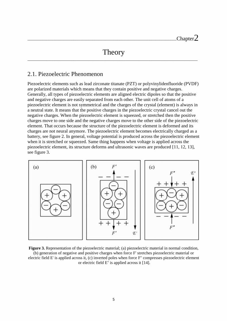
2.1. Piezoelectric Phenomenon

Piezoelectric elements such as lead zirconate titanate (PZT) or polyvinylidenfluoride (PVDF)

are polarized materials which means that they contain positive and negative charges.

Generally, all types of piezoelectric elements are aligned electric dipoles so that the positive

and negative charges are easily separated from each other. The unit cell of atoms of a

piezoelectric element is not symmetrical and the charges of the crystal (element) is always in

a neutral state. It means that the positive charges in the piezoelectric crystal cancel out the

negative charges. When the piezoelectric element is squeezed, or stretched then the positive

charges move to one side and the negative charges move to the other side of the piezoelectric

element. That occurs because the structure of the piezoelectric element is deformed and its

charges are not neural anymore. The piezoelectric element becomes electrically charged as a

battery, see figure 2. In general, voltage potential is produced across the piezoelectric element

when it is stretched or squeezed. Same thing happens when voltage is applied across the

piezoelectric element, its structure deforms and ultrasonic waves are produced [11, 12, 13],

see figure 3.

Figure 3. Representation of the piezoelectric material; (a) piezoelectric material in normal condition,

(b) generation of negative and positive charges when force F' stretches piezoelectric material or

electric field E' is applied across it, (c) inverted poles when force F'' compresses piezoelectric element

or electric field E'' is applied across it [14].

6

2.2. Generation and Detection of Ultrasonic Waves by Piezoelectric

Elements

A piezoelectric element is a mechanical device which can convert energy from one form to

another one, see figure 4. It converts electrical energy to mechanical or mechanical energy to

electrical [11]. Piezoelectric elements are used in all ultrasonic transducers.

Figure 4. The vibration of the piezoelectric element in two different cases [11].

The above figure shows that the piezoelectric element produces ultrasonic waves when

voltage is applied across it. The piezoelectric elements also produce voltage when ultrasonic

waves hit its surface. The ultrasonic waves press the surface of the piezoelectric element

which can lead to generation of voltage.

A piezoelectric element can generate ultrasound waves when DC voltage is quickly applied

and removed from the two electrodes of the piezoelectric element. The applied voltage makes

the piezoelectric element change its size and its surface starts to vibrate up and down, at that

moment the piezoelectric element will resonate at its resonant frequency [15].

The process of generation of ultrasonic waves from a piezoelectric element is the following:

Electrical pulse Mechanical vibration Ultrasonic wave generation

On the other hand, when the ultrasound waves hit the surface of the piezoelectric element at

that moment its surface starts to vibrate and that results in generating of electrical pulse, see

figure 3. The process of detection of ultrasonic waves in an ultrasonic transducer is the

following:

Reflected ultrasonic wave Mechanical vibration Electrical pulse

7

The delivered power from the ultrasonic transducer is expressed in milliwatts and it is

dependent on the applied voltage across the piezoelectric element with almost no current is

applied to the transducer.

2.3. Speed and Wavelength

The definition of ultrasonic speed through a material is the vibration of the kinetic energy

passed from one particle to another particle. The ultrasonic speed is different in various

materials, see table 3. When the particles in a material are too close to each other and tighter

their bonds then the ultrasonic speed is increased in that material. The studies show that the

velocity of the ultrasonic waves in different samples is depending on many factors e.g. size of

the sample, elastic properties, density, porosity and how many different minerals are

embedded in the sample [22, 23].

The ultrasonic speed in a material affects the beam spread of the ultrasonic waves when it

propagates through the sample. A higher ultrasonic speed gives a wider beam spread while a

slower ultrasonic speed gives a narrower beam spread.

Table 3. Different speeds of the ultrasound waves in varied materials [24].

Material Speed of sound in m/s

Dry air 331

Water 1540

Bright drawn steel 6100

Aluminum 6320

Silicone 1485

Rock-Marble 3810

Glass 4540

Gold 3240

Rubber 60

The speed of the ultrasonic wave in a homogenous material is dependent on two factors; the

elastic properties of the material and its density as shown in the following formula:

𝑐 = √𝐶ₑ

𝜌 (2)

where Ce is the elastic property of the material and 𝜌 is the density [20]. The elastic property

describes the stiffness of the material.

Furthermore, the wavelength of sound is defined as one cycle of a wave. It is dependent on

the frequency of the waves and its velocity. A high frequency gives a short wavelength while

a low frequency gives a long wave length. The relation between the ultrasonic wavelength

and its speed is expressed in the following formula:

= 𝑐𝑡 =𝑐

𝑓 (3)

8

where t is the period and c is the velocity of the soundwave [20].

2.4. Propagation of Ultrasonic Waves

The propagation of ultrasound waves in a material is dependent on the following factors:

1)The acoustic impedance Z (Rayls) of the material is the ultrasonic waves propagate through

it. The formula of the acoustic impedance of a material is calculated by:

𝑍 = 𝑝o· 𝑐 (4)

where the 𝑝o is the mean density of the material and c is the velocity of the ultrasonic wave in

the material [20]. When the ultrasonic waves penetrate through two different materials with

different acoustic impedances then some of the ultrasonic waves reflected to the transducer

[17].

The percentage of the reflected ultrasound waves R is calculated by

𝑅 =(𝑍₂−𝑍₁)2

(𝑍₁+𝑍₂)2 100 % (5)

where 𝑍2is the acoustic impedance of the second material while 𝑍1 is the acoustic impedance

of the first material [20]. The percentage of the transmitted ultrasound waves 𝑇 through the

material is calculated by following formula [20]:

𝑇 = 1 − 𝑅 (6)

2)The attenuation of the ultrasonic wave when it propagates through a material. The

propagation leads to loss of energy of the propagated waves because of scattering and

absorption in the material, that can cause reducing of the intensity of the propagated

ultrasonic waves. The definition of the attenuation is described as scattering of ultrasonic

waves plus damping of ultrasonic waves in the examined material. Scattering is the reflection

of ultrasonic waves in random directions while absorption is the conversion of ultrasonic

energy to other types of energy. The effect of scattering and absorption in a specific material

is called attenuation [20].

The internal friction and thermal conductivity of the examined material can lead to energy

losses of the propagated waves because of its energy is converted to thermal heat. The

scattering of waves is more relevant for metals because they made of randomly oriented

grains. If the size of one grain is 20 times less than the wavelength of the ultrasonic wave,

then the relation between the attenuation coefficient and the frequency becomes linear [25].

Generally, each material has its own attenuation coefficient, see table 4. The higher the

attenuation coefficient, the higher the attenuation of the propagated ultrasonic waves inside

the material, see figures 5, 6.

9

Table 4. Attenuation coefficients for different materials at 1 MHz frequency [18].

Material Attenuation coefficient (dB/(MHz cm))

Bright drawn steel 434·10-7

Aluminum 434·10-8

Marble 9.5

Rock 15

When ultrasonic waves propagate through two materials with different sound velocities, at

that moment the amplitude of the ultrasonic waves decrease if the second material has a

lower sound velocity than the first material. The lower sound velocity you have, the shorter

the wavelength you get, see equation (3). That is why the attenuation is greater in the second

material.

Furthermore, the temperature of some materials can give to an increased attenuation. Gases

and liquids with hot temperature decrease the velocity of ultrasonic propagation and that

causes a higher attenuation but it is vice versa in water [25].

Figure 5. Attenuation in different thicknesses of a bright drawn steel sample and an aluminum

sample.

10

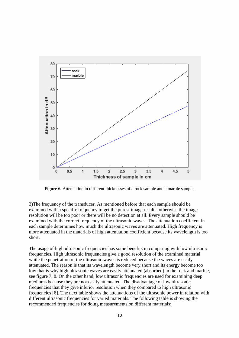
Figure 6. Attenuation in different thicknesses of a rock sample and a marble sample.

3)The frequency of the transducer. As mentioned before that each sample should be

examined with a specific frequency to get the purest image results, otherwise the image

resolution will be too poor or there will be no detection at all. Every sample should be

examined with the correct frequency of the ultrasonic waves. The attenuation coefficient in

each sample determines how much the ultrasonic waves are attenuated. High frequency is

more attenuated in the materials of high attenuation coefficient because its wavelength is too

short.

The usage of high ultrasonic frequencies has some benefits in comparing with low ultrasonic

frequencies. High ultrasonic frequencies give a good resolution of the examined material

while the penetration of the ultrasonic waves is reduced because the waves are easily

attenuated. The reason is that its wavelength become very short and its energy become too

low that is why high ultrasonic waves are easily attenuated (absorbed) in the rock and marble,

see figure 7, 8. On the other hand, low ultrasonic frequencies are used for examining deep

mediums because they are not easily attenuated. The disadvantage of low ultrasonic

frequencies that they give inferior resolution when they compared to high ultrasonic

frequencies [8]. The next table shows the attenuations of the ultrasonic power in relation with

different ultrasonic frequencies for varied materials. The following table is showing the

recommended frequencies for doing measurements on different materials:

11

Table 5. The recommended ultrasound frequencies on varied materials [26].

Material

Recommended frequency

Notes

Metals in general

0.1-15-MHz

It depends on the thickness

of the metal. If it is too thick

then low frequency is

preferred otherwise higher

frequency is preferred.

Aluminum 1-MHz Even higher frequencies

give reliable results.

Wood 50-200-kHz

Silicon in breast 3.5-5-MHz

Rock

50-700-kHz

High frequencies are

disapproved because the

attenuation is too high.

Water

1-MHz

Higher frequencies

are not highly attenuated

in water.

Glass 1-MHz

Lucite (a transparent plastic) 1-MHz

Steel 900 kHz Even with higher

frequencies are possible to

be applied.

12

Figure 7. Attenuation with different frequencies in aluminum and bright drawn steel samples.

Figure 8. Attenuation with different frequencies in rock and marble samples.

13

2.5. Basic Design of an Ultrasonic Transducer

The main idea behind the design of ultrasonic transducers is the shape and thickness of the

piezoelectric element of the transducer. The shape of the piezoelectric element defines how

much is the transmitted ultrasonic waves are focused while the thickness of the piezoelectric

element defines the frequency of the transmitted ultrasonic waves, no matter what kind of

piezoelectric material it is.

The frequency of the ultrasonic waves determines the spread shape of the ultrasonic waves. A

low frequency of ultrasonic waves gives a wider field while a high frequency gives a

narrower ultrasonic field [16], see figure 9. If the diameter of the piezoelectric element is

large in the transducer, that will provide a better focusing of the transmitted ultrasonic waves.

Figure 9. Two beam spread of ultrasound waves for two transducers with the same diameter. The

above beam shows the spread of 1-MHz transducer while the below beam shows

the spread of 5-MHz transducer.

The beam angle of the ultrasonic waves, see figure 10, can be calculated by using the

following formula:

sin() = 1.2𝑉

𝐷𝑓 (7)

Figure 10. Beam spread of ultrasonic waves from an ultrasonic transducer [16].

14

where is the beam divergence angle as shown in figure 5, 𝑉 is ultrasound velocity in the

examined material, 𝐷 is the diameter of the ultrasonic transducer and 𝑓 is the frequency of

the transducer [16].

The diameter of the piezoelectric element is important in making of ultrasonic transducers. In

figure 11, the shape of the piezoelectric element is in circular form. It shows that a larger

diameter of the piezoelectric element gives a better focusing of the transmitted ultrasonic

waves in the examined material.

Figure 11. Beam spread angle of the transmitted ultrasound waves. shows half the beam spread

angle of the transmitted ultrasound waves in aluminum and marble from a transducer of 1-MHz

frequency with different diameters of the piezoelectric element.

On the other hand, different thicknesses of piezoelectric elements give rise to different

ultrasonic frequencies of ultrasonic transducers. In the below figure, it is obvious that the

thickness of 10-MHz transducer is less than the thickness of 1-MHz transducer of PVDF-

films. The thickness of the piezoelectric element should be /2 of the transmitted ultrasonic

waves to achieve the desired resonance frequency, where is the wavelength of the

transmitted ultrasonic waves.

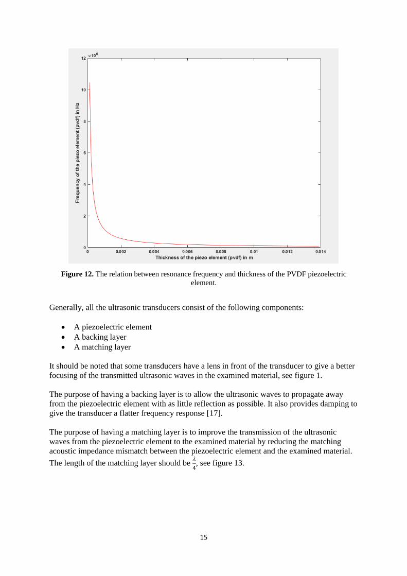
15

Figure 12. The relation between resonance frequency and thickness of the PVDF piezoelectric

element.

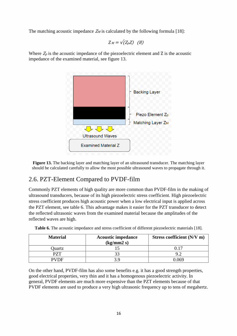
Generally, all the ultrasonic transducers consist of the following components:

A piezoelectric element

A backing layer

A matching layer

It should be noted that some transducers have a lens in front of the transducer to give a better

focusing of the transmitted ultrasonic waves in the examined material, see figure 1.

The purpose of having a backing layer is to allow the ultrasonic waves to propagate away

from the piezoelectric element with as little reflection as possible. It also provides damping to

give the transducer a flatter frequency response [17].

The purpose of having a matching layer is to improve the transmission of the ultrasonic

waves from the piezoelectric element to the examined material by reducing the matching

acoustic impedance mismatch between the piezoelectric element and the examined material.

The length of the matching layer should be

4, see figure 13.

16

The matching acoustic impedance ZM is calculated by the following formula [18]:

𝑍M = √(ZpZ) (8)

Where Zp is the acoustic impedance of the piezoelectric element and Z is the acoustic

impedance of the examined material, see figure 13.

Figure 13. The backing layer and matching layer of an ultrasound transducer. The matching layer

should be calculated carefully to allow the most possible ultrasound waves to propagate through it.

2.6. PZT-Element Compared to PVDF-film

Commonly PZT elements of high quality are more common than PVDF-film in the making of

ultrasound transducers, because of its high piezoelectric stress coefficient. High piezoelectric

stress coefficient produces high acoustic power when a low electrical input is applied across

the PZT element, see table 6. This advantage makes it easier for the PZT transducer to detect

the reflected ultrasonic waves from the examined material because the amplitudes of the

reflected waves are high.

Table 6. The acoustic impedance and stress coefficient of different piezoelectric materials [18].

Material Acoustic impedance

(kg/mm2 s)

Stress coefficient (N/V m)

Quartz 15 0.17

PZT 33 9.2

PVDF 3.9 0.069

On the other hand, PVDF-film has also some benefits e.g. it has a good strength properties,

good electrical properties, very thin and it has a homogenous piezoelectric activity. In

general, PVDF elements are much more expensive than the PZT elements because of that

PVDF elements are used to produce a very high ultrasonic frequency up to tens of megahertz.

17

On the other hand, the efficiency of all piezoelectric elements is determined by comparing the

amount of the input power to the transducer to the amount of the output energy of the

transducer. In case when the amount of the output power is close to the amount of the input

power, it means that the piezoelectric element is efficient otherwise it is less efficient.

Because of low efficiency, the produced image by using such piezoelectric element is less

accurate and reliable [15]. The common advantage of all piezoelectric elements that they

offer a wide dynamic range and they are broadband materials.

2.7. Frequency Response of Piezoelectric Elements

The Frequency of an ultrasonic transducer is dependent on the thickness of the piezoelectric

element. In general terms, a thin piezoelectric element has a higher resonance frequency than

a thick piezoelectric element of the same composition material, volume, and shape [15,19].

The following equation calculates the resonance frequency of the piezoelectric element [12]:

𝑓 =𝑣

2𝑡ℎ (9)

Where f is frequency of ultrasonic waves, v is the velocity of ultrasonic waves in the

piezoelectric element (usually v = 2300 m/s for PVDF) and th is the thickness of the

piezoelectric element in meter. A piezoelectric element vibrates with a wavelength that is

double its thickness, that is why a piezoelectric element is cut to a thickness that it is half the

desired wavelength of the emitted ultrasonic wave [8,13,20]. The relation between resonance

frequency of the PVDF piezoelectric element and its thickness is shown in figure 7.

2.8. Circular and Square PVDF-film

The golden coated circular and square PVDF-film will be investigated in this thesis work, see

figure 14.

Figure 14. Illustration of circular and square PVDF-film.

The biggest difference between using of circular and square PVDF-films is that the near field

length of the piezoelectric element is different in circular and square piezoelectric elements.

For a circular piezoelectric element, its near field is calculated by the following formula [21]:

𝑁 =D2𝑓

4 𝑣 (10)

Where D is the diameter of the piezoelectric element, f is the frequency of the transducer and

v is the sound velocity in the examined sample. While the formula for the near field length of

a square piezoelectric element is the following [30]:

𝑁 =1.35 D2𝑓

4 𝑣 (11)

18

Where D is the side length of the piezoelectric element. The near field defined as the area

where it is difficult to evaluate flaws in the examined sample. The fluctuation in sound

intensity in this area causes an unordered acoustic oscillation of the ultrasonic waves [21].

The longer is the near field, the worse is the transducer. The following table is showing some

values of the near field length for two shapes of piezoelectric transducers:

Table 7. Near field length of circular and square PVDF transducers.

Circular transducers Square transducers

Diameter in cm Near field length in

cm

Side length in cm Near field length in

cm

1 0.40 1 0.53

1.25 0.62 1.25 0.67

1.5 0.89 1.5 0.80

The above table shows different values of parameter D in the equations (10) and (11). The

frequency of the transducers is 1-MHz and the ultrasonic testing was applied on an aluminum

piece. It is obvious that the higher the diameter is, the longer is the near field length. It is

preferred to use a circular transducer but for much bigger values of parameter D it is more

efficient to use a square transducer as emitters, because of its near field length is less

compared to the circular ones.

2.9. Ultrasound Couplant

The first enemy of ultrasonic waves is air; Air has a low acoustic impedance as shown in

table 8. The ultrasonic waves reflect when they encounter air. The acoustic impedance of the

ultrasonic couplant should be close to the acoustic impedance of the transducer beam to allow

the ultrasonic waves to propagate through it and them to the examined material. There should

be no air bubbles in the ultrasound couplant when doing experiments otherwise it is not

efficient to use ultrasound couplant [27]. Here is an example of the reflected ultrasonic waves

between air and aluminum boundary.

Reflected waves (air to aluminum boundary) = (0.0004−17.33)²

(0.0004+17.33)²100 % = 99.9%

This means that 99.9% of the transmitted ultrasonic waves are reflected when they encounter

air between the transducer and the aluminum sample. Ultrasound couplant has a very close

acoustic impedance to water. Ultrasound couplant makes the ultrasonic waves easily

propagated through the couplant and on to the examined material. It means that the reflected

ultrasonic waves are much minimized [27].

Reflected waves (couplant to aluminum boundary) = (2.42−17.33)2

(2.42+17.33)2 100 % = 56.99 %

This means that 56.99 % of the transmitted ultrasonic waves reflect when they go through the

ultrasonic couplant before they enter the examined aluminum sample.

19

Table 8. The acoustic impedance of different materials [28].

Medium Acoustic impedance

Z (MRayls)

Air 0.0004

Water 1.48

Aluminum 17.33

Ultrasound couplant

(Glycerin)

2.42

The acoustic impedance of the ultrasound couplant is required to be less than the acoustic

impedance of the examined material. When that constraint is satisfied, then the ultrasonic

waves easily penetrate through the examined sample otherwise there is no penetration of the

ultrasonic waves occurs inside the sample.

The propagation of ultrasonic waves is affected by the attenuation coefficient of the

examined sample. The more ultrasonic waves propagate through the sample, the more their

amplitude is decreasing, see figure 15. The reason for that is the ultrasonic waves are more

attenuated and scattered when they go deeper in the sample.

Figure 15. The propagation of ultrasonic waves in an aluminum sample.

20

_______________________________________________________________________Chapter3

Tools and Setups _________________________________________________________________________________

3.1. Tools from Lecoeur Electrique Company

Lecoeur Electronique is a company which works with ultrasonic testing and producing of

ultrasonic devices for researching purposes. US-key is an ultrasound device which is

manufactured by Lecoeur Electronique. The US-key can be used to investigate the thickness

and physical properties of various materials such as rock, aluminum, plastic, rubber, wood

etc. The device has two channels, one for transmitting ultrasonic waves and the other one to

receive the reflected waves (echoes) from the examined material. The device is connected to

a computer via an USB connector. The power supply from the US-key to the ultrasonic

transducer (ultrasound probe) is 5 Voltage DC [29]. Any channel of the US-key could be

used in two modes at the same time as a transmitter and a receiver, see figure 16.

Figure 16. The connection of the US-key to the computer and to the ultrasound transducer (probe)

[29].

The basic idea behind the US-key is that it transmits a pulse via an ultrasonic transducer with

a specific frequency and plots the reflected pulse in a xy-plane. Different ultrasonic

transducers were bought separately from the US-key device. The US-key device can be used

with Lecoeur software or with MATLAB. The plotted figures in the Lecoeur software show

the amplitude of the reflected pulse on the y-axes while the x-axes represent the distance in

mm or the time in µs.

21

3.1.1. Linear Array Transducer by Using Two US-keys and an

Interface Module

The first method for designing of the linear array transducer is by using an interface module

and two US-keys. The interface module is a multi-channel block which can be connected to

one US-key as shown in the below figure [30].

Figure 17. The interface module connected to one US-key [30].

Two US-keys and the interface module are supposed to be used to build up the linear array

transducer. The idea of the linear array transducer is shown in the following figure:

Figure 18. The layout of the linear array transducer with one emitter and two receivers with US-keys.

There the connecting box is an electric circuit with resistors which was designed to connect

two US-keys. The connecting box reduces the input voltage from the left US-key to the right

US-key.

The linear array transducer is considered to have one industrial transducer as an ultrasonic

emitter and two PVDF-films as ultrasonic receivers. The shape of the PVDF- film is decided

to be circular of 1 cm of diameter, but then it was changed to be 1.5 cm in diameter. The

reason for choosing 1.5 cm in diameter is to detect higher amplitude of the reflected

22

ultrasonic waves when doing measurements. The examined material is decided to be

aluminum because it gave readable results.

3.2. Linear Array Transducer by Using a Generator and an

Oscilloscope

The second method for designing of the linear array transducer is by using a generator and an

oscilloscope. The generator was used to power two industrial 1-MHz transducers. The

oscilloscope was connected to three PVDF-film receivers to detect the ultrasonic waves

which propagate through the examined sample. The difference between using US-keys

compared with generator and oscilloscope is that the oscilloscope does display and save the

raw data of the measurements while the US-key does not do that.

The two industrial transducers are connected to two power channels in the generator. Three

PVDF-film receivers, each one is connected to a channel in the oscilloscope. Each channel

gives its own raw data which can be saved and handled in MATLAB. All the three PVDF-

film receivers are made of circular shape with 1.5 cm in diameter. The reason for that is to

detect a much signal as possible.

The two industrial transducers transmit ultrasonic waves with same frequency at 1-MHz. The

active frequency of the three PVDF-film receivers is at 10-MHz but the PVDF-film could

detect even low frequency as 1-MHz without difficulties.

Below is the setup of the linear array transducer:

Figure 19. The layout of the linear array transducer with two emitters and three receivers

By using generator and oscilloscope.

23

_______________________________________________________________________Chapter4

Measurements _________________________________________________________________________________

Here are all the measurements which were done to decide which sample is the most

appropriate to be examined in the linear array transducer. The measurements are done with

industrial transducers, PZT transducers and handmade transducers of PVDF-films with

different shapes and sizes. The results of the measurements are illustrated in the result part of

this thesis report.

Initially, greace was used as couplant. It is a good conductive medium to enable a tight bond

between the transducer and the sample, but later it was changed to another couplant called

Mollas. Mollas couplant was less messy and easier to clean it out.

The meaning of using industrial transducers in some cases is to make sure that the measured

results from using PVDF-films are acceptable. The results from PVDF-films were compared

to the industrial ones. In the other hand, the meaning of using PZT piezoelectric elements is

just to develop acknowledge and experience in different piezoelectric elements.

4.1 Measurements by US-key with Lecoeur Software

All the measurements in this section were done with the Lecoeur software by using a single

US-key device. Different transducers and piezoelectric elements were connected to the US-

key in different combinations as the tables below show.

Table 9. Measurements on a manufactured steel specimen by using 5-MHz transducer with other

combinations. Grease was used as couplant.

Type of test Material

5-MHz transducer as an emitter and a PVDF-film as a receiver

Manufactured steel

5-MHz transducer as a receiver and a PVDF-film as an emitter

5-MHz transducer as an emitter and as a receiver

5-MHz transducer as an emitter and a PZT (1-MHz) as a

receiver

5-MHz transducer as a receiver and a PZT (1-MHz) as an

emitter

5-MHz transducer as an emitter and a PZT (5-MHz) as a

receiver

5-MHz transducer as a receiver and a PZT (5-MHz) as an

emitter

24

Table 10. Measurements on a rock specimen by using 5-MHz transducer with other combinations.

Grease was used as couplant.


5-MHz transducer as an emitter and a PZT (1-MHz) as a receiver

Rock 5-MHz transducer as a receiver and a PZT (1-MHz) as an emitter



5-MHz transducer as a receiver and a PZT (2-MHz) as an emitter



Table 11. Measurements on an aluminum specimen by using 5-MHz transducer with other




Aluminum







Table 12. Measurements on a silicone specimen by using 5-MHz transducer with other combinations.




Silicone


5-MHz transducer as an emitter and a PZT (2 MHz) as a receiver

5-MHz transducer as a receiver and a PZT (2 MHz) as an emitter


5-MHz transducer as a receiver and a PZT(5-MHz) as an emitter

5-MHz transducer as a receiver and as an emitter


25

Table 13. Measurements on a marble specimen by using 5-kHz transducer with other combinations.



500-kHz transducer as an emitter and as a receiver

Marble the 500-kHz transducer as an emitter and a PZT (1-MHz) as a receiver

500-kHz transducer as a receiver and a PZT (1-MHz) as an emitter

Table 14. Measurements on a rock specimen by using 5-kHz transducer with other combination.



500-kHz transducer as an emitter and a PVDF-film as a receiver

Rock 500-kHz transducer as a receiver and a PVDF-film as an emitter


500-kHz transducer as an emitter and a PZT (1-MHz) as a receiver


Table 15. Measurements on a metal specimen by using 5-kHz transducer with other combinations.




Manufactured

steel

500-kHz transducer as an emitter and a PZT (5-MHz) as a receiver



Table 16. Measurements on an aluminum specimen by using 5-kHz transducer with other




Aluminum 500-kHz transducer as an emitter and a PZT (1-MHz) as a receiver



Table 17. Measurements on a silicone specimen by using 5-kHz transducer with other combinations.




Silicone 500-kHz transducer as an emitter and a PZT (1-MHz) as a receiver


26

Table 18. Measurements on different specimen by using 5-kHz transducer as emitter and receiver.

Mollas was used as couplant.


500-kHz transducer as an emitter and as a receiver Marble

500-kHz transducer as an emitter and as a receiver Rock

500-kHz transducer as an emitter and as a receiver Manufactured steel

500-kHz transducer as an emitter and as a receiver Aluminum

500-kHz transducer as an emitter and as a receiver Silicone

500-kHz transducer as an emitter and as a receiver Plastic

Table 19. Measurements on different specimen by using square shapes of PVDF-films

as emitter and receiver. Mollas was used as couplant.


PVDF (1.5*1.5 cm2) as emitter and receiver Aluminum

PVDF (1.5*1.5 cm2) as emitter and receiver Manufactured steel

PVDF (1.5*1.5 cm2) as emitter and receiver Silicone

PVDF (1.25*1.25 cm2) as emitter and receiver Aluminum

PVDF (1.25*1.25 cm2) as emitter and receiver Manufactured steel

PVDF (1.25*1.25 cm2) as emitter and receiver Silicone

PVDF (1*1 cm2) as emitter and receiver Aluminum

PVDF (1*1 cm2) as emitter and receiver Manufactured steel

PVDF (1*1 cm2) as emitter and receiver Silicone

Table 20. Measurements on different specimen by using square shapes of PVDF-films

with other combinations. Mollas was used as couplant.



Bright drawn steel PVDF (1*1 cm2) as emitter and receiver

PVDF (1*1 cm2) as receiver and (1.25*1.25 cm2) as emitter

PVDF (1*1 cm2) as receiver and (1.25*1.25 cm2) as emitter Aluminum

PVDF (1*1 cm2) as receiver and (1.25*1.25 cm2) as emitter Silicone

Table 21. Measurements on different specimen by using square and circular shapes of PVDF-films.

Mollas was used as couplant.


PVDF (Diameter of 1.5cm, 1.25cm and 1cm)

as emitter and receiver

Aluminum, bright

drawn Steel, and

Silicone

PVDF (1*1 cm2) as receiver and (1.25*1.25 cm2) as emitter Aluminum

27

Table 22. Measurements on a silicone specimen by using two circular shapes of PVDF-films

as emitter and receiver. Mollas was used as couplant.


Pvdf (1*1 cm2) as emitter and receiver silicone

Pvdf (1.5*1.5 cm2) as emitter and receiver silicone

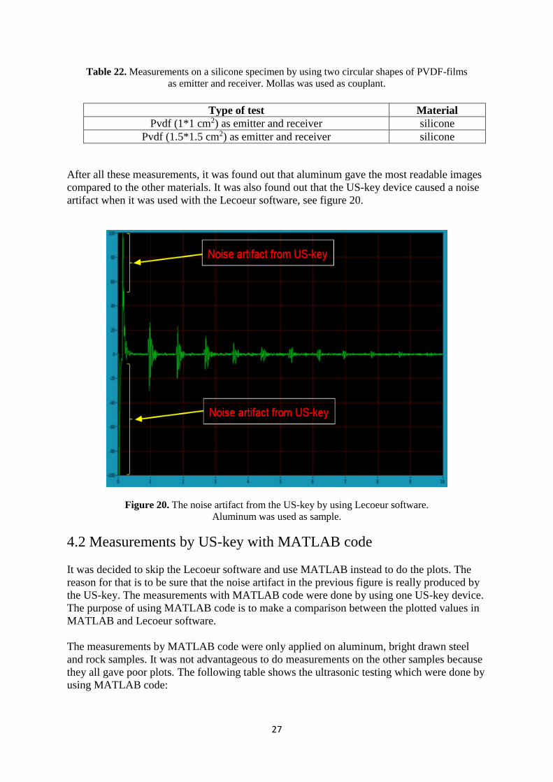
After all these measurements, it was found out that aluminum gave the most readable images

compared to the other materials. It was also found out that the US-key device caused a noise

artifact when it was used with the Lecoeur software, see figure 20.

Figure 20. The noise artifact from the US-key by using Lecoeur software.

Aluminum was used as sample.

4.2 Measurements by US-key with MATLAB code

It was decided to skip the Lecoeur software and use MATLAB instead to do the plots. The

reason for that is to be sure that the noise artifact in the previous figure is really produced by

the US-key. The measurements with MATLAB code were done by using one US-key device.

The purpose of using MATLAB code is to make a comparison between the plotted values in

MATLAB and Lecoeur software.

The measurements by MATLAB code were only applied on aluminum, bright drawn steel

and rock samples. It was not advantageous to do measurements on the other samples because

they all gave poor plots. The following table shows the ultrasonic testing which were done by

using MATLAB code:

28

Table 23. Measurements on different specimen by MATLAB code.

Measurements were done with Mollas couplant.


PVDF (circular of 1 cm in diameter) as emitter and receiver

Aluminum,

bright drawn

steel and rock



1-MHz transducer as an emitter and 1-MHz as a receiver

PVDF (circular of 1 cm in diameter) one as emitter and another one

as receiver

PVDF (circular of 1 cm in diameter) as emitter and 5 MHz

transducer as receiver and vice versa

PVDF (circular of 1 cm in diameter) as emitter and 1-MHz

transducer as receiver and vice versa

PVDF (square of 1 cm, 1.25 cm and 1.5 cm in length) as emitter and

receiver

PVDF (square of 1 cm, 1.25 cm and 1.5 cm in length) one as emitter

and another one as receiver

The plots from MATLAB software were quite like the plots from the Lecoeur software. In

the following figure, it shows the noise artifact which is created by the US-key device. For

the following plot, it was used two industrial transducers of 1-MHz, one as emitter and the

other one as receiver.

29

Figure 21. The noise artifact from the US-key by using MATLAB code.

Aluminum was used as sample.

The above picture shows the noise artifact which was produced when one US-key device was

used to do plots in MATLAB. Even here, the noise artifact confirms that it is produced by the

US-key.

4.3 Measurements by a Generator and an Oscilloscope

Until now it was found that the US-key device is not the proper device to be used to do

ultrasonic testing because it creates a noise artifact in the beginning of the plot, see figure 23,

24. The plan of the project was changed to use generator and oscilloscope to do ultrasonic

testing.

The advantage of using generator and oscilloscope that there is no noise is creating by these

devices and you can save the raw data of each measurement. But at the same time the

oscilloscope is very sensitive when it takes measurements.

In the next page, table 24 shows some measurements which were done by using the generator

and the oscilloscope. The idea behind these measurements is to determine the best way to

connect the PVDF-films to the oscilloscope to achieve as good plots as possible.

30

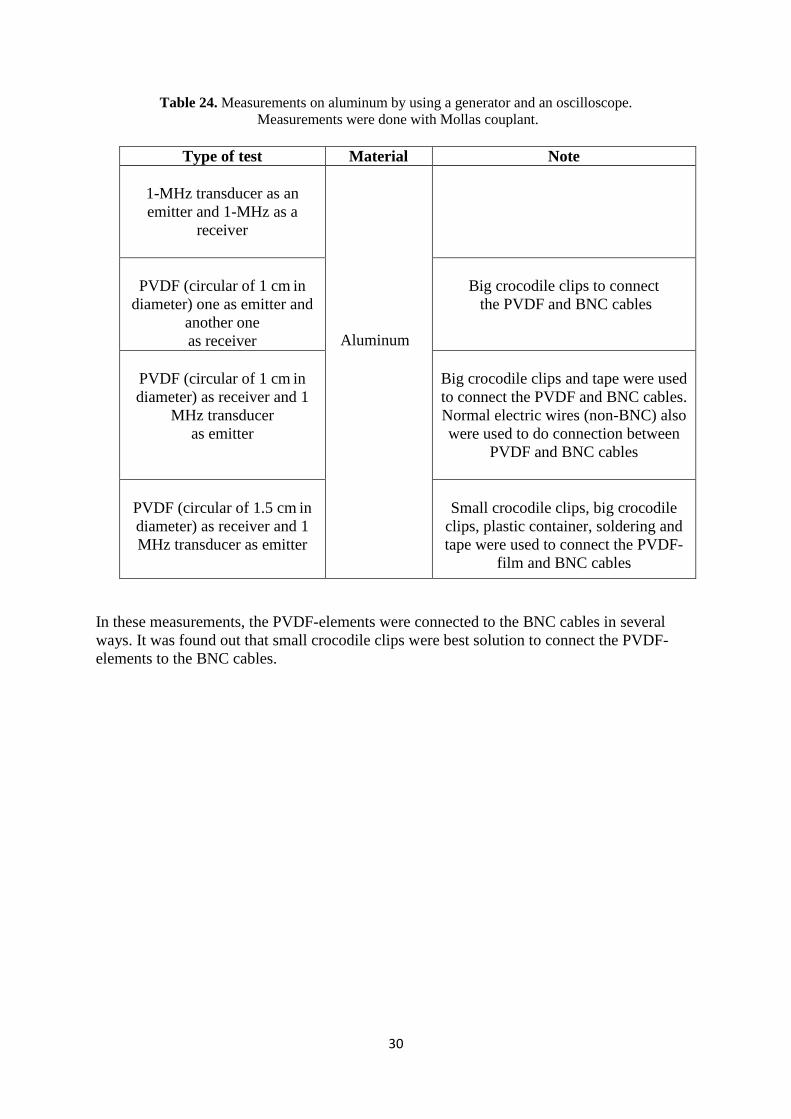
Table 24. Measurements on aluminum by using a generator and an oscilloscope.

Measurements were done with Mollas couplant.

Type of test Material Note

1-MHz transducer as an

emitter and 1-MHz as a

receiver

Aluminum

PVDF (circular of 1 cm in

diameter) one as emitter and

another one

as receiver

Big crocodile clips to connect

the PVDF and BNC cables

PVDF (circular of 1 cm in

diameter) as receiver and 1

MHz transducer

as emitter

Big crocodile clips and tape were used

to connect the PVDF and BNC cables.

Normal electric wires (non-BNC) also

were used to do connection between

PVDF and BNC cables

PVDF (circular of 1.5 cm in

diameter) as receiver and 1

MHz transducer as emitter

Small crocodile clips, big crocodile

clips, plastic container, soldering and

tape were used to connect the PVDF-

film and BNC cables

In these measurements, the PVDF-elements were connected to the BNC cables in several

ways. It was found out that small crocodile clips were best solution to connect the PVDF-

elements to the BNC cables.

31

_______________________________________________________________________Chapter5

Results and Discussion _________________________________________________________________________________

The achieved results in measurements of different samples fit with the theory, because the

samples with high attenuation coefficient gave poor images while the samples with low

attenuation coefficient gave legible images. The quality of the images which were taken by

using the PVDF-films gave better results than the PZT. The PZT-elements which were used

in this thesis work have low quality. The low quality of the PZT-elements could be because

they were manufactured by using cheap chemical materials. This means that PVDF-film is

vibrating more when it detects ultrasonic waves while the PZT does not vibrate as much as

the PVDF-film.

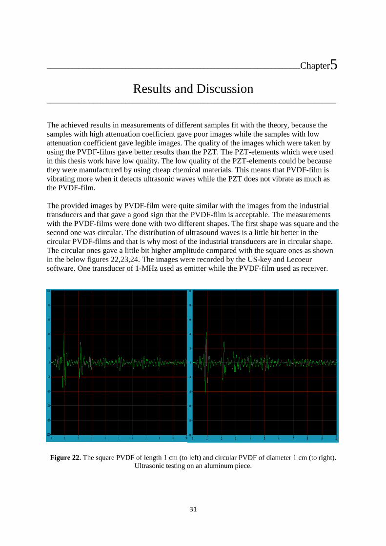
The provided images by PVDF-film were quite similar with the images from the industrial

transducers and that gave a good sign that the PVDF-film is acceptable. The measurements

with the PVDF-films were done with two different shapes. The first shape was square and the

second one was circular. The distribution of ultrasound waves is a little bit better in the

circular PVDF-films and that is why most of the industrial transducers are in circular shape.

The circular ones gave a little bit higher amplitude compared with the square ones as shown

in the below figures 22,23,24. The images were recorded by the US-key and Lecoeur

software. One transducer of 1-MHz used as emitter while the PVDF-film used as receiver.

Figure 22. The square PVDF of length 1 cm (to left) and circular PVDF of diameter 1 cm (to right).

Ultrasonic testing on an aluminum piece.

32

Figure 23. The square PVDF of length 1.25 cm (to left) and circular PVDF of diameter 1.25 cm (to

right). Ultrasonic testing on an aluminum piece.

As shown in the above pictures that the received ultrasonic waves have a little higher

amplitude with the circular PVDF-films compared to the square PVDF-films.

In the following figure, it shows the differences between circular PVDF-film of 1.5 cm in

diameter and square PVDF-film of length 1.5 cm:

Figure 24. The square PVDF of length 1.5 cm (to left) and circular PVDF of diameter 1.5 cm (to

right). Ultrasonic testing on an aluminum piece.

It shows that the both gave almost the same result. It was decided later to choose circular

PVDF-films of diameter 1.5 cm as receiver for making of the linear array transducer because

it gave a little bit higher amplitude, see figure 25.

33

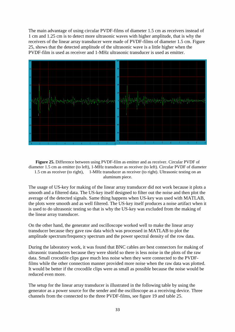
The main advantage of using circular PVDF-films of diameter 1.5 cm as receivers instead of

1 cm and 1.25 cm is to detect more ultrasonic waves with higher amplitude, that is why the

receivers of the linear array transducer were made of PVDF-films of diameter 1.5 cm. Figure

25, shows that the detected amplitude of the ultrasonic wave is a little higher when the

PVDF-film is used as receiver and 1-MHz ultrasonic transducer is used as emitter.

Figure 25. Difference between using PVDF-film as emitter and as receiver. Circular PVDF of

diameter 1.5 cm as emitter (to left), 1-MHz transducer as receiver (to left). Circular PVDF of diameter

1.5 cm as receiver (to right), 1-MHz transducer as receiver (to right). Ultrasonic testing on an

aluminum piece.

The usage of US-key for making of the linear array transducer did not work because it plots a

smooth and a filtered data. The US-key itself designed to filter out the noise and then plot the

average of the detected signals. Same thing happens when US-key was used with MATLAB,

the plots were smooth and as well filtered. The US-key itself produces a noise artifact when it

is used to do ultrasonic testing so that is why the US-key was excluded from the making of

the linear array transducer.

On the other hand, the generator and oscilloscope worked well to make the linear array

transducer because they gave raw data which was processed in MATLAB to plot the

amplitude spectrum/frequency spectrum and the power spectral density of the row data.

During the laboratory work, it was found that BNC cables are best connectors for making of

ultrasonic transducers because they were shield so there is less noise in the plots of the raw

data. Small crocodile clips gave much less noise when they were connected to the PVDF-

films while the other connection manner provided more noise when the raw data was plotted.

It would be better if the crocodile clips were as small as possible because the noise would be

reduced even more.

The setup for the linear array transducer is illustrated in the following table by using the

generator as a power source for the sender and the oscilloscope as a receiving device. Three

channels from the connected to the three PVDF-films, see figure 19 and table 25.

34

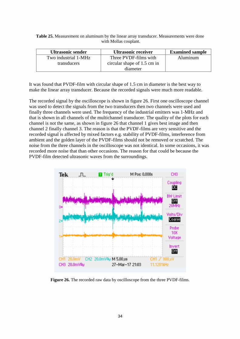
Table 25. Measurement on aluminum by the linear array transducer. Measurements were done

with Mollas couplant.

Ultrasonic sender Ultrasonic receiver Examined sample

Two industrial 1-MHz

transducers

Three PVDF-films with

circular shape of 1.5 cm in

diameter

Aluminum

It was found that PVDF-film with circular shape of 1.5 cm in diameter is the best way to

make the linear array transducer. Because the recorded signals were much more readable.

The recorded signal by the oscilloscope is shown in figure 26. First one oscilloscope channel

was used to detect the signals from the two transducers then two channels were used and

finally three channels were used. The frequency of the industrial emitters was 1-MHz and

that is shown in all channels of the multichannel transducer. The quality of the plots for each

channel is not the same, as shown in figure 26 that channel 1 gives best image and then

channel 2 finally channel 3. The reason is that the PVDF-films are very sensitive and the

recorded signal is affected by mixed factors e.g. stability of PVDF-films, interference from

ambient and the golden layer of the PVDF-films should not be removed or scratched. The

noise from the three channels in the oscilloscope was not identical. In some occasions, it was

recorded more noise that than other occasions. The reason for that could be because the

PVDF-film detected ultrasonic waves from the surroundings.

Figure 26. The recorded raw data by oscilloscope from the three PVDF-films.

35

The raw data recorded signal has noise for the three channels as shown above. The reason for

that is already mentioned. The frequency distribution spectrum and power spectral density of

each channel in the linear array transducer are not 100% identical to each other as shown

below.

Figure 27. The recorded signal by first oscilloscope channel with its amplitude spectrum

and power spectral density. It was plotted in MATLAB.

Figure 28. The same recorded signal by second oscilloscope channel with its amplitude spectrum

and power spectral density measured in MATLAB.

Figure 29. The same recorded signal by third oscilloscope channel with its amplitude spectrum

and power spectral density measured in MATLAB.

36

The frequency spectrum of the three channels is a little bit identical but the power spectral

density of all the channels is not the same. The reason for that could be because the

connection between the PVDF-films and the BNC cables is not perfect. The frequency

spectrums above show that 1-MHz frequency is recorded as it was expected, because the

emitters are using 1-MHz frequency. There are also other frequencies are detected which

could be frequencies of radio channels.

In conclusion, here is an illustration of different ultrasonic parameters which are calculated in

this thesis work. The acoustical parameters are calculated by using some standard equations.

Firstly, the velocity of sound in an aluminum piece is calculated by

𝑐 =𝑙

𝑡 (12)

There t is time between sending and receiving ultrasonic wave and l is length of the

aluminum. The distance between the sender and emitter is called l. The time is calculated by

the Lecoeur software and the length of the sample is calculated by a ruler.

𝑐 =0.0285 𝑚𝑒𝑡𝑒𝑟

0.000004676 𝑠𝑒𝑐𝑜𝑛𝑑 = 6095 m/s

The theoretical value of sound velocity in aluminum is 6320 m/s. The absorption or

attenuation of ultrasonic waves in the aluminum is calculated by

𝐴𝑡𝑡𝑒𝑛𝑢𝑎𝑡𝑖𝑜𝑛 = 𝑎 · 𝑙 · 𝑓 (13)

There 𝑎 is the attenuation coefficient of the examined material and 𝑓 is the frequency of the

transmitted ultrasonic wave, there 𝑓 is chosen to be 1-MHz.

𝐴𝑡𝑡𝑒𝑛𝑢𝑎𝑡𝑖𝑜𝑛 = 0.00000434 𝑑𝐵

𝑀𝐻𝑧 𝑐𝑚· 2.85 𝑐𝑚 · 1 𝑀𝐻𝑧 = 0.000012369 𝑑𝐵

The acoustic impedance Z of aluminum is calculated by this formula:

𝑍 = 𝑝ₒ · 𝑐 = 2.7 gram/cm3 · 6320000 cm/s = 17064000 g/cm2s

Finally, the transmission of ultrasonic waves from the transducer can be called as contentious

because the common mode of operation is pulsed at a given period (generally 4 to 5000 times

a second), it can be continuous but caution must be taken so the piezoelectric element does

not become over temperature of 150 C.

37

_______________________________________________________________________Chapter6

Conclusions _________________________________________________________________________________

The conclusion of this thesis work is that the quality of ultrasonic images depends on three

main factors. The first factor is the resonance frequency of the transducer, the second factor is

type of the piezoelectric element and the third factor is the attenuation coefficient of the

examined sample. It is important to use the right frequency when measuring on different

samples. The thickness of the piezoelectric material determines the frequency of the

transmitted ultrasonic waves. It is also important to use the right couplant when doing

ultrasonic testing. The acoustic impedance of the couplant is important to be less than the

acoustic impedance of the examined sample.

The PVDF-film of diameter 1.5 cm gave the most accurate images compared to the other

PVDF-films of 1 cm and 1.25 cm in diameter when they were used as receivers. But on the

other hand, when they were used as emitters, the amplitudes of the images were little bit

reduced. The investigated PVDF-film is better to be used for receiving of ultrasonic waves.

When the circular PVDF-film of 1.5 cm in diameter was used as emitter or receiver, the

images were much better than those with the circular PVDF-film of 1 cm and 1.25 cm in

diameter.

Furthermore, the square PVDF-films were not good as the circular ones. The amplitude of the

images from the circular ones were a little bit higher compared to the square ones. The square

PVDF-films are usually used for testing of weld integrity. It is more applied for angular

ultrasonic transducers because it is more appropriate for scanning of large areas.

The aluminum was the best sample of the all examined samples. The attenuation coefficient

of the aluminum is much lower compared with the other samples, that made the images from

the aluminum much more accurate compared to the other samples. The produced images in

different samples ranked from best to worst, are:

Aluminum

Bright drawn steel

Manufactured steel

Silicone

Plastic

Rock

Marble

On the other hand, the linear array transducer was not successful when it was done by using

two US-keys and an interface module. The noise artifact from the US-keys caused us to

change the plan by using generator and oscilloscope instead.

38

The setup for the generator and oscilloscope is also called linear array transducer. Generally,

the main benefit of using generator and oscilloscope is that they gave the raw data of the

measurements while the Lecoeur Electronique software did not provide the raw data of the

measurements.

The aluminum piece was used in all trails in this setup. The reason is its low attenuation

coefficient. In the setup, there were two industrial transducers used of 1-MHz frequency used

as emitters. 1-MHz transducers provide a wider propagation of ultrasonic waves. It was not

efficient to use the PVDF-film as ultrasonic emitter in the setup because the frequency of the

PVDF-film is 10-MHz which is too high. High frequencies are less penetrated in the

materials. The frequency of the PVDF-film is calculated by equation (9) as following:

f = 2300 𝑚/𝑠

2∗110 µ𝑠 = 10 MHz

In the linear array transducer when generator and oscilloscope were used, the best way to

connect PVDF-films to BNC cables is by using small crocodile clips. Small crocodile clips

gave much less noise when the measurements were done. Here is the order of the connectors

that were applied to connect PVDF-films to the BNC cables, ranked from best to worst:

Small crocodile clips

Big crocodile clips

Electricity tape conductor

Normal electric wires

Soldering

Finally, the images from the three channels in the oscilloscope did not provide more details

about the aluminum sample. There was a wide variance between the recorded raw data from

each channel in the oscilloscope. The reason for that may be that the connections between the

PVDF-films and BNC cables were not enough good or the PVDF-film is too sensitive which

makes the measurements too difficult to proceed.

6.1. Future work

This thesis work was made to do an experimental work of how to design a linear array

transducer by using two US-keys. When this setup did not work, which was not expected

with Lecoeur Electronique software, then MATLAB was used instead. The MATLAB code

from Lecoeur company was improved to make the linear array transducer. Because of the

artifact that the US-key did create then it was decided to move on and use generator and

oscilloscope to extract the raw data in MATLAB instead of using US-keys and Lecoeur

software. The future work can be summarized in the following points:

Different thickness of PVDF -films can be tested on different samples. Each thickness

is related to a specific frequency, that means it will be more informative if the PVDF-

films with low frequency are used to measure on rocks or marble

Use LABVIEW instead of generator and buy the required equipment for that

39

_______________________________________________________________________Chapter7

References _________________________________________________________________________________

[1] Explainthatstuff, " Ultrasound," Explainthatstuff, May 2015. [Online]. Available:

http://www.explainthatstuff.com/ultrasound.html. [Accessed September 2016].

[2] D. Merton, "Diagnostic Medical Ultrasound Technology: A Brief Historical Review,"

Journal of Diagnostic Medical Sonography, vol. 13, no. 5, supplement, pp. 10s-23s,

September 1997.

[3] D. N. J.J. Wild, "Use of high-frequency ultrasonic waves for detecting changes of texture

in living tissues," The Lancet, vol. 257, no. 6656, pp. 655-657, 1951.

[4] Yale-New Haven Teachers Institute, " Imaging the Human Body with Ultrasound"

Elisabet O. Orville, 2016. [Online]. Available:

http://teachersinstitute.yale.edu/curriculum/units/1983/7/83.07.06.x.html. [Accessed

September 2016].

[5] Strål Säkerhet Myndigheten, "Ultraljud," Strål Säkerhet Myndigheten, July 2007.

[Online]. Available: http://www.stralsakerhetsmyndigheten.se/start/Vard/Ultraljud/.

[Accessed September 2016].

[6] CancerQuest, "Introduction to Ultrasound Imaging," CancerQuest, July 2007. [Online].

Available: http://www.stralsakerhetsmyndigheten.se/start/Vard/Ultraljud/. [Accessed

September 2016].

[7] hyperphysics, "Ultrasonic sound," hyperphysics, 1999. [Online]. Available:

http://hyperphysics.phy-astr.gsu.edu/hbase/sound/usound.html. [Accessed September 2016].

[8] Radiopaedia.org, " Ultrasound Frequencies," Radiopaedia.org, 2005-2016. [Online].

Available: https://radiopaedia.org/articles/ultrasound-frequencies. [Accessed September

2016].

[9] e. a. P. Huskins, Diagnostic ultrasound physics and equipment, Cambridge: Cambridge

University Press, 2010.

[10] Mitopencourseware, "Nanomaker," Mitopencourseware,2001-2016. [Online]. Available:

https://ocw.mit.edu/courses/electrical-engineering-and-computer-science/6-s079-nanomaker-

spring-2013/labs/MIT6_S079S13_slides09.pdf. [Accessed September 2016].

[11] Ultrasonic Technology, " Basic Principle of Medical Ultrasonic Probes (Transducer)",

2016. [Online]. Available: http://www.ndk.com/en/sensor/ultrasonic/basic02.html. [Accessed

September 2016].

40

[12] Explainthatstuff, " Piezoelectricity," Woodford C, July 2016. [Online]. Available:

http://www.explainthatstuff.com/piezoelectricity.html. [Accessed September 2016].

[13] NDT Resource Center, " Piezoelectric Transducers," Woodford C, July 2016. [Online].

Available: https://www.nde-

ed.org/EducationResources/CommunityCollege/Ultrasonics/EquipmentTrans

/piezotransducers.htm. [Accessed September 2016].

[14] Jansson, A. (2007). Piezoelectric Generation and Damping of Extensional Waves in

Bars. Uppsala, Geotryckeriet.

[15] Measurement Specialties, "Piezo Film Sensors Technical Manual," [Online]. Available:

https://www.sparkfun.com/datasheets/Sensors/Flex/MSI-techman.pdf. [Accessed October

2016].

[16] El-Reedy, M. (2013). Concrete and Steel Construction. New York, CRC press.

[17] Åberg, M. (1999). Wave Propagation and Damage in Composite Laminates. Stockholm,

KTH Högskoletryckeriet.

[18] BME 240, " Ultrasound Background," Patel N, June 2009. [Online]. Available:

http://bme240.eng.uci.edu/students/09s/patelnj/Ultrasound_for_Nerves/Ultrasound_Backgrou

nd.html. [Accessed October 2016].

[19] APC international, Ltd, " Determining Resonance Frequency," APC international, Ltd,

2016. [Online]. Available: https://www.americanpiezo.com/knowledge-center/piezo-

theory/determining-resonance-frequency.html. [Accessed September 2016].

[20] Qifa Z, Sienting L, Dawei W, and K. Kirk S, Piezoelectric films for high frequency

ultrasonic transducers in biomedical applications. Prog Mater Sci. 2011 Feb; 56(2): 139–174.

doi: 10.1016/j.pmatsci.2010.09.001

[21] NDT Education Resource Center, Ultrasonic Inspection-near field calculation. [Online].

Available:

https://www.nde-ed.org/GeneralResources/Formula/UTFormula/near_field/near.htm.

[Accessed April 2017].

[22] M. Khandelwal and T. N. Singh, “Correlating Static Properties of Coal Measures Rocks

with P-Wave Velocity,” International Journal of Coal Geology, Vol. 79, No.

[23] S. Kahraman, “A Correlation between P-Wave Velocity, Number of Joints and Schmidt

Hammer Rebound Number,” International Journal of Rock Mechanics and Mining Sciences,

Vol. 38, No. 5, 2001, pp. 729-733. doi:10.1016/S1365-1609(01)00034-X

[24] Olympus, "Material Sound Velocities". [Online]. Available: http://www.olympus-

ims.com/en/ndt-tutorials/thickness-gage/appendices-velocities/. [Accessed November 2016].

[25] Kocis, S, and Figura, Z. (1996). Ultrasonic Measurements and Technologies. London,

Chapman & Hall.

41

[26] ASTM international, "Ultrasonic Testing," ASTM international, [Online]. Available:

https://www.astm.org/BOOKSTORE/DS68/pg41.pdf. [Accessed September 2016].

[27] HealDove, " Why it Is Important to Use Gel in Ultrasound", April 2016. [Online].

Available: https://healdove.com/health-care-industry/aquasonic_ultrasound_gel. [Accessed

September 2016].

[28] Radiopaedia.org, " Acoustic Impedance," Radiopaedia.org, 2005-2016. [Online].

Available: https://radiopaedia.org/articles/acoustic-impedance. [Accessed September 2016].

[29] Lecoeur Electronique, 2010. [Online]. Available:

http://www.lecoeur-electronique.net/cariboost_files/us-key_r4_0.pdf. [Accessed November

2016].

[30] Lecoeur Electronique, 2010. [Online]. Available:

http://www.lecoeur-electronique.net/wa_files/interface_module_en_r3_0.pdf. [Accessed

January 2016].

42

__________________________________________________________________________________

Appendix I __________________________________________________________________________________

Abbreviated MATLAB code:

clc;

clear;

% Attenuation in steel and aluminum

alfa=0.0000434/1000000; % Attenuation constant (dB/(MHz*cm))

of steel

l=[0:1:5]; % Sample length in mm from 0 cm to 5 cm

f=1000000; % Frequency at 1 MHz

Attenuation = alfa*l*f; % Attenuation formula

plot(l,Attenuation,'g')

% title('Attenuation in different thickness of steel');

set(gca,'FontName','Arial','FontSize',10,'FontWeight','Bold');

xlabel('Thickness of sample in cm');

ylabel('Attenuation in dB');

set(gca, 'XLim',[0 5]);

hold on


of aluminum

l=[0:1:5]; % Sample length in mm from 0 mm to 5 cm



plot(l,Attenuation,'m')

% title('Attenuation in different thickness of aluminum');


xlabel('Thickness of sample in cm');



legend('steel','aluminum','Location','northwest')

alfa=9.5/1000000; % Attenuation constant (dB/(MHz*cm)) of rock

l=[0:1:5]; % Sample length in cm from 0.10 cm to 4 cm



figure(7)

plot(l,Attenuation,'b')

% title('Attenuation in different thickness of rock');


xlabel('Thickness of rock in cm');



43

alfa=15/1000000; % Attenuation constant (dB/(MHz*cm)) of

marble

l=[0:1:5]; % Sample length in mm from 0 cm to 10 cm



figure(8)

plot(l,Attenuation,'k')

% title('Attenuation in different thickness of marble');


xlabel('Thickness of marble in cm');



clc;

clear;

alfa=15/1000000; % Attenuation constant (dB/(MHz*cm)) for

marble

l=0.4; % Sample length in cm

f=[500000:500000:15000000]; % Frequencies


plot(f,Attenuation,'k')

hold on

alfa=9.5/1000000; % Attenuation constant (dB/(MHz*cm)) for

rock


f=[500000:500000:15000000]; % Frequencies


plot(f,Attenuation,'b')

hold on


for aluminum


f=[500000:500000:15000000]; % Frequencies


plot(f,Attenuation,'m')

hold on


for steel


f=[500000:500000:15000000]; % Frequencies


plot(f,Attenuation,'g')

hold on

set(gca, 'XLim',[400000 16000000]);

% title('Frequency attenuation in different materials');

xlabel('Different frequencies');


legend ('aluminum','steel')


legend('marble','rock')

44

clc;

clear;

dt=1/8000; % seconds per sample

st=0.004; % stop time in second

t = (0:dt:st-dt)'; % time interval

f = 500000; % frequency at 500 kHz

x = cos(2*pi*f*t);

figure;

plot(t,x,'b');

xlabel('Time in seconds');

ylabel('Wave amplitude')


title('Signal with short wavelength at 500 kHz');

zoom xon;

dt=1/8000; % seconds per sample

st=0.004; % stop time in second

t = (0:dt:st-dt)'; % time interval

f = 50000; % frequency at 500 Hz

x = cos(2*pi*f*t);

figure;

plot(t,x,'r');

xlabel('Time in seconds');

ylabel('Wave amplitude')


title('Signal with long wavelength at 500 Hz');

zoom xon;

% the piezo element is a pvdf

clc;

clear;

th=[0.00011:0.0001:0.014]; % thickness of the piezo element in

meter

c=2300; % acoustic velocity of the crystal

(piezo element)

f=c./(2*th); % frequency of the piezo element in Hz

plot(th,f,'r')


xlabel('Thickness of the piezo element (pvdf) in m');

ylabel('Frequency of the piezo element (pvdf) in Hz')

% title('The relation between resonance frequency and

thickness of the piezo element');

%zoom xon;

clc;

clear;

f=1000000; % frequenct at 1 MHz

c=[300:100:1800]; % ultrasound speed

45

l = c./f; % wavelength formula

plot(c,l,'b')


% title('Relation between wavelength and ultrasound speed');

xlabel('Different ultrasound speeds in m/s');

ylabel('Wavelength in m');

xlim([250 1850])

ylim([0 0.002])

clc;

clear;

v=6320; % velocity in aluminum in m/s

f=1000000; % % Frequency at 1 MHz

d=[0.015:0.001:0.025]; % diameter of the piezo element in m

theta=asind((1.2*v)./(d*f)); % theta is the beam divergence

angle from centerline to point where signal is at half

strength

plot(r,theta,'m')

xlabel('Diameter of the piezo element in m')

ylabel('Beam divergence angle in degrees')

hold on

v=5115; % velocity in marble in m/s

f=1000000; % % Frequency at 1 MHz

d=[0.015:0.001:0.025]; % diameter of the piezo element in m

theta=asind((1.2*v)./(d*f)); % theta is the beam divergence

angle from centerline to point where signal is at half

strength

plot(r,theta,'k')

xlabel('Diameter of the piezo element in m')

ylabel('Beam divergence angle (\theta) in degrees')


legend('aluminum','marble')

L=2500; %signal length

variable = dlmread('C:\Users\ali\Desktop\Oscillo\exCh33.csv');

% Access the time variable

time = variable(: , 1);

% Access the voltage which measured on the oscilloscope

voltage = variable(: , 2);

figure(1)

plot (time,voltage)

title('Recorded signal by one PVDF-plate')

xlabel('time')

ylabel('voltage')

46

ylim([-0.015 0.025]); % just interested in frequencies between

0 and 3 MHz

% Fast fourier transform of the voltage to plot different

frequencies

Y = fft(voltage);

P2 = abs(Y/L);

P1 = P2(1:L/2+1);

P1(2:end-1) = 2*P1(2:end-1);

Fs=1/(time(2,1)-time(1,1));

f = Fs*(0:(L/2))/L;

figure(2)

plot(f,P1)

xlim([0 3000000]); % just interested in frequencies between 0

and 3 MHz

ylim([0 0.002]);

title('Amplitude spectrum of voltage')

xlabel('frequency')

ylabel('voltage')

figure(3)

powerspectral= pwelch(voltage);

plot(10*log10(powerspectral));

title('Power spectral density')

ylabel('dB')

xlabel('rad/sample')

xlim([0 510]);

% propagation of ultrasonic waves in the linear array

transducer

with two US-keys

plot([1 4.2], [2 2.5],'w')

hold on

plot([1 4.2], [2 1.5],'w')

ylim([0 4]);

xlim([0 5]);

scatter(1,2,80,'filled')

scatter(4.2,2.5,60,'filled','k')

scatter(4.2,1.5,60,'filled','k')

set(gca,'xtick',[])

set(gca,'ytick',[])

title('Propagation of ultrasonic waves');

th = linspace( pi/7, -pi/7, 10);

R = 0.35; %radius of the circle

47

x = R*cos(th)+0.95;

y = R*sin(th)+2;

plot(x,y,'g'); axis equal;

th1 = linspace( pi/6, -pi/6, 10);


x = R*cos(th1)+1.35;

y = R*sin(th1)+2;




x = R*cos(th2)+1.75;

y = R*sin(th2)+2;




x = R*cos(th3)+2.45;

y = R*sin(th3)+2;


text(0.2,2.5,' One ultrasonic emitter','FontSize',10)

text(3.3,0.8,' Two ultrasonic receivers','FontSize',10)

% the MATLAB code for the linear array transducer by using US-

key

clear all;

loadlibrary('C:\DLL_USKEY_x64\Ap_int_usb.dll','C:\DLL_USKEY_x6

4\Ap_int_usb.h','alias','ApintUsb')

Err_Code(1) = int16(1);

Product = uint32(1);

Channel = uint32(0);

Out1(1) = uint16(1);

Out2(1) = uint16(1);

Out3(1) = uint16(1);

Out4(1) = uint16(1);

Out5(1) = uint16(1);

Out6(1) = uint16(1);

Len(1) = int16(3900);

Array(Len) = uint16(0);

%Function = 'RunExeX32';

Err_Code=calllib('ApintUsb','ApintUsb',Product,Channel,'RunExe

X32',0,0,0,0,0,0,Out1,Out2,Out3,Out4,Out5,Out6,Array,Len);

% Loading x32 to x64 resident

48

%%%%%%%%%%%%%%%%%%%%%%%%%%%%%%%%%%%%%%%%%%%%%%%%%%%%%%%%%%%

% Loading DLL and Init US-key %

%%%%%%%%%%%%%%%%%%%%%%%%%%%%%%%%%%%%%%%%%%%%%%%%%%%%%%%%%%%

calllib('ApintUsb','ApintUsb',Product,Channel,'Init

usb',0,0,0,0,0,0,Out1,Out2,Out3,Out4,Out5,Out6,Array,Len)

% Loadind DLL

calllib('ApintUsb','ApintUsb',Product,Channel,'load

configuration',1,0,0,0,0,0,Out1,Out2,Out3,Out4,Out5,Out6,Array

,Len) % Init US-Key

%%%%%%%%%%%%%%%%%%%%%%%%%%%%%%%%%%%

% US-Key Transmitter management %

%%%%%%%%%%%%%%%%%%%%%%%%%%%%%%%%%%%

PRF = 0.5;

% PRF (KHz)

% special value PRF = 0.07 (external sync)

Tension = 120;

% Voltage (Volts)

% from 30 to 230 Volts

Largeur_Pulse = 5;

Retard_Pulse = 0;

% Pulse

calllib('ApintUsb','ApintUsb',Product,Channel,'Prf',PRF,0,0,0,

0,0,Out1,Out2,Out3,Out4,Out5,Out6,Array,Len)

calllib('ApintUsb','ApintUsb',Product,Channel,'voltage',Tensio

n,0,0,0,0,0,Out1,Out2,Out3,Out4,Out5,Out6,Array,Len)

calllib('ApintUsb','ApintUsb',Product,Channel,'width',Largeur_

Pulse,0,0,0,0,0,Out1,Out2,Out3,Out4,Out5,Out6,Array,Len)

calllib('ApintUsb','ApintUsb',Product,Channel,'pulse

delay',Retard_Pulse,0,0,0,0,0,Out1,Out2,Out3,Out4,Out5,Out6,Ar

ray,Len)

%%%%%%%%%%%%%%%%%%%%%%%%%%%%%%%%%%%%

% US-Key Receiver management %

%%%%%%%%%%%%%%%%%%%%%%%%%%%%%%%%%%%%

Filtre = 2;

% Filters

49

Mode = 0;

% Mode

Gain = 20;

% Gain 0

Retard_Num = 0;

% Scale

Freq_Num = 1; %

Sampling frequencies

calllib('ApintUsb','ApintUsb',Product,Channel,'filter/mode',Fi

ltre,Mode,0,0,0,0,Out1,Out2,Out3,Out4,Out5,Out6,Array,Len)

calllib('ApintUsb','ApintUsb',Product,Channel,'Gain',Gain,0,0,

0,0,0,Out1,Out2,Out3,Out4,Out5,Out6,Array,Len)

calllib('ApintUsb','ApintUsb',Product,Channel,'scale

delay',Retard_Num,0,0,0,0,0,Out1,Out2,Out3,Out4,Out5,Out6,Arra

y,Len)

calllib('ApintUsb','ApintUsb',Product,Channel,'samplingfreqmod

e',Freq_Num,Mode,0,0,0,0,Out1,Out2,Out3,Out4,Out5,Out6,Array,L

en)

%%%%%%%%%%%%%%%%%%%%%%%%%%%%%%%%%%%%%%%%%%%%%%%

% US-Key Gates management %

%%%%%%%%%%%%%%%%%%%%%%%%%%%%%%%%%%%%%%%%%%%%%%%

Num_Porte = 1;

% Gate

Pos_Porte = 10;

% Gate

Larg_Porte = 5;

% Gate

Seuil_Porte = 30;

%Threshold (%)

calllib('ApintUsb','ApintUsb',Product,Channel,'gate

position',Num_Porte,Pos_Porte,0,0,0,0,Out1,Out2,Out3,Out4,Out5

,Out6,Array,Len)


width',Num_Porte,Larg_Porte,0,0,0,0,Out1,Out2,Out3,Out4,Out5,O

ut6,Array,Len)


hight',Num_Porte,Seuil_Porte,0,0,0,0,Out1,Out2,Out3,Out4,Out5,

Out6,Array,Len)

calllib('ApintUsb','ApintUsb',Product,Channel,'relays',bin2dec

('000'),0,0,0,0,0,Out1,Out2,Out3,Out4,Out5,Out6,Array,Len)%

Alarms (On appearence or vanish)

50

%%%%%%%%%%%%%%%%%%%%%%%%%%%%%%%%%%%%%%%%%%%%%%%%%

% US-Key A-scan %

%%%%%%%%%%%%%%%%%%%%%%%%%%%%%%%%%%%%%%%%%%%%%%%%%

Type_Donnees = 0;

Nb_Echantillons = 3900; %

Number of samples

Forme_Onde = 0;

%%%

calllib('ApintUsb','ApintUsb',Product,Channel,'Ascan',Type_Don

nees,0,Nb_Echantillons,Forme_Onde,0,0,Out1,Out2,Out3,Out4,Out5

,Out6,Array,Len)

calllib('ApintUsb','ApintUsb',Product,Channel,'Scale A-scan

counter',Nb_Echantillons/2,0,0,0,0,0,Out1,Out2,Out3,Out4,Out5,

Out6,Array,Len)

tic

matrix=zeros(100,3900);

for i=1:100

[Err_Code Function Out1 Out2 Out3 Out4 Out5 Out6 Array Len] =

calllib('ApintUsb','ApintUsb',Product,Channel,'A-

scan',Type_Donnees,0,Nb_Echantillons,Forme_Onde,0,0,Out1,Out2,

Out3,Out4,Out5,Out6,Array,Len);

matrix(i,:)=Array;

pause(5/1000);

figure(1)

plot(Array(1:Len));drawnow;

end

toc

%%plot(Array)

xlabel('Echantillons');

ylabel('Valeur');

calllib('ApintUsb','ApintUsb',Product,Channel,'KillExeX32',0,0

,0,0,0,0,Out1,Out2,Out3,Out4,Out5,Out6,Array,Len)

51

__________________________________________________________________________________

Appendix II __________________________________________________________________________________

Here are some selected pictures of the measurements which were done by using a single US-

key and Lecoeur software.

Manufactured steel: Measurements with 5 MHz transducer as emitter and circular PVDF-film

of diameter 1 cm as receiver.

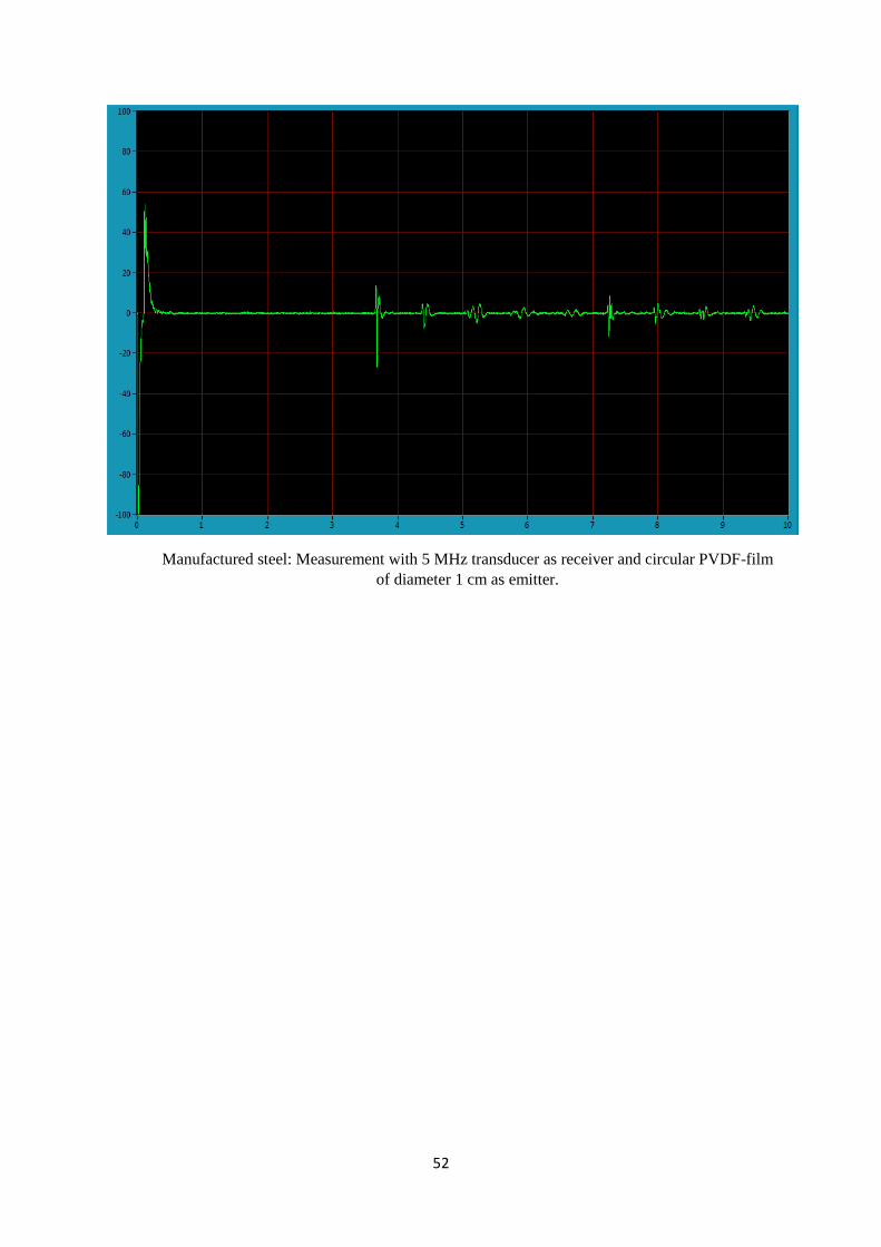
52

Manufactured steel: Measurement with 5 MHz transducer as receiver and circular PVDF-film

of diameter 1 cm as emitter.

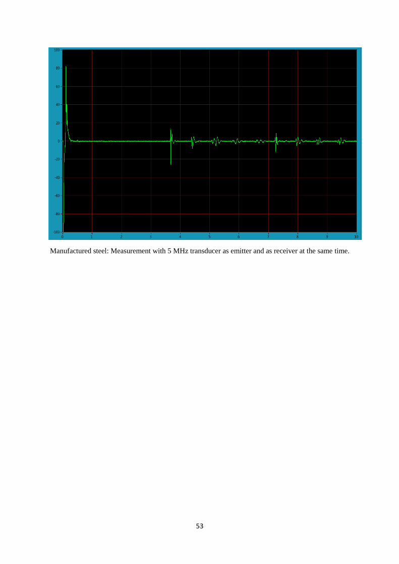
53

Manufactured steel: Measurement with 5 MHz transducer as emitter and as receiver at the same time.

54

Manufactured steel: Measurement with 500 kHz transducer as emitter and as receiver at the same

time.

Aluminum: Measurement with 5 MHz transducer as emitter and PVDF-film of diameter 1 cm

as receiver.

55

Aluminum: Measurement with 5 MHz transducer as receiver and circular PVDF-film

of diameter 1 cm as emitter.

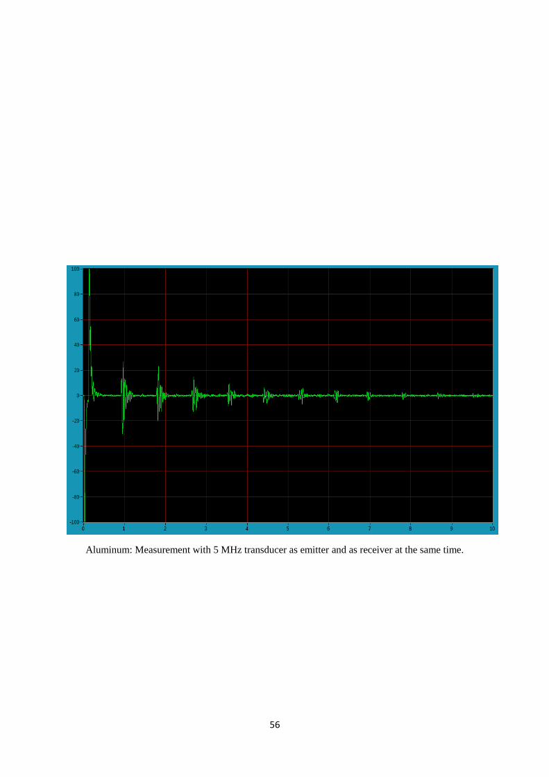
56

Aluminum: Measurement with 5 MHz transducer as emitter and as receiver at the same time.

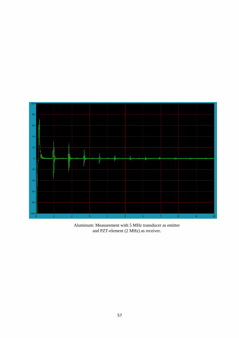
57

Aluminum: Measurement with 5 MHz transducer as emitter

and PZT-element (2 MHz) as receiver.

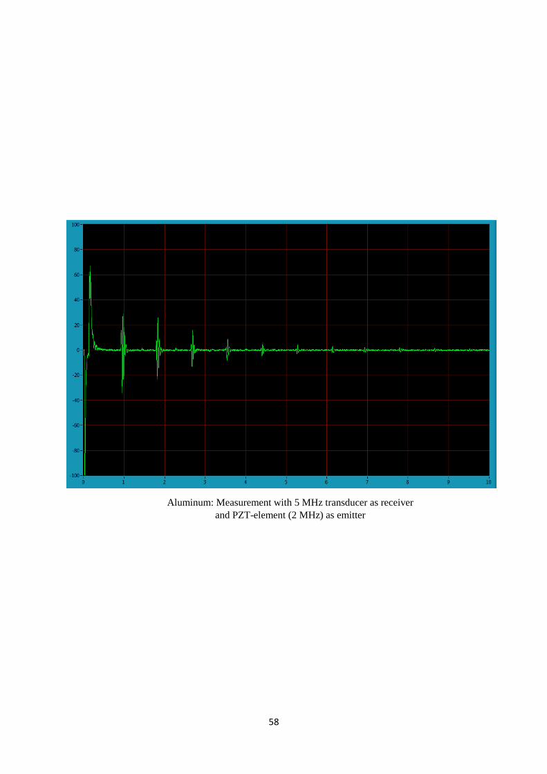
58

Aluminum: Measurement with 5 MHz transducer as receiver

and PZT-element (2 MHz) as emitter

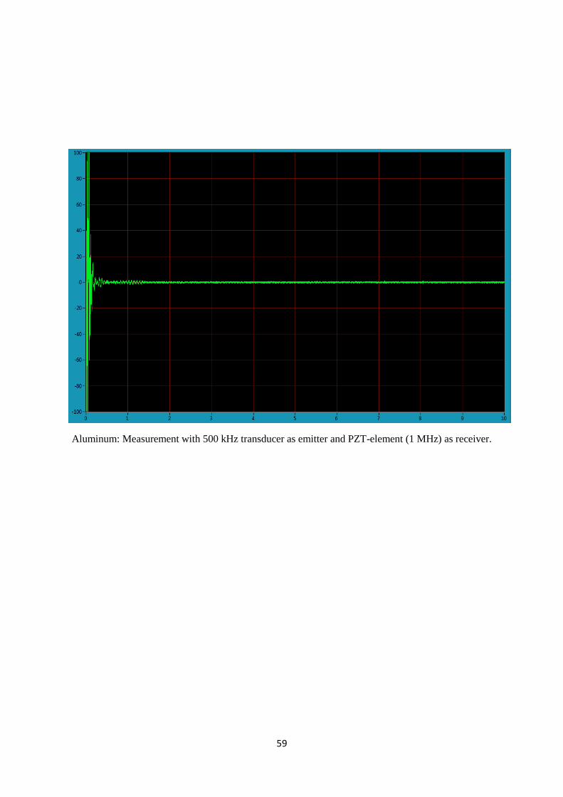
59

Aluminum: Measurement with 500 kHz transducer as emitter and PZT-element (1 MHz) as receiver.

60

Aluminum: Measurement with 500 kHz transducer as receiver and PZT-element (1 MHz) as emitter.

61

Aluminum: Measurement with 500 kHz transducer as emitter and as receiver at the same time.

Rock: Measurement with 500 kHz transducer as emitter and as receiver at the same time.

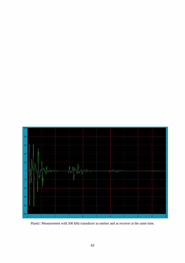
62

Plastic: Measurement with 500 kHz transducer as emitter and as receiver at the same time.

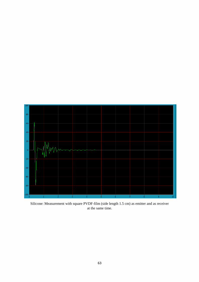
63

Silicone: Measurement with square PVDF-film (side length 1.5 cm) as emitter and as receiver

at the same time.

64

Silicone: Measurement with circular PVDF-film (diameter 1.5 cm) as emitter and as receiver

at the same time.

Bright drawn steel: Measurement with circular PVDF-film (diameter 1.25 cm) as emitter and as

receiver at the same time.

65

Bright drawn steel: Measurement with circular PVDF-film (diameter 1.5 cm) as emitter and as

receiver at the same time.

an investigation on pvdf piezoelectric … investigation on pvdf piezoelectric elements and linear...

Documents