an investigation of the information propagation and ... · an investigation of the information...
TRANSCRIPT

NASA Contractor Report 189143
//V-3 7 /
An Investigation of the InformationPropagation and Entropy TransportAspects of Stifling MachineNumerical Simulation
Louis F. Goldberg
University of Minnesota
Minneapolis, Minnesota
April 1992
Prepared for
Lewis Research Center
Under Service Contract Order C-22742-P
NANANational Aeronautics and
Space Administration
(NASA-CR-189143) AN [NV£STI_,AIIO_'I OF
INFORMATION PROPAGAT[_N AND ENTROPY
IRANSPOPI A£PFCTS OF STIRLING MACHINE
NUMERICAL SIMULATION Final Report
(Minnesota Univ.) 52 p
THE
G3134
N72-27975
Uncl as
0104066
https://ntrs.nasa.gov/search.jsp?R=19920018732 2018-09-06T20:15:41+00:00Z

i
CO_TENTS
NOTATION
INTRODUCTION
PART A:
A.I
A.2
A.3
A.4
A.5
A.6
A.7
INFORMATION PROPAGATION
Introduction
Analytic Background
A Non-Pressure-Linked Symmetric Integral Formulation
Explicit Solution Limlting_orm
n-Step Implicit Temporal Integration Algorithm
Results
Conclusion
PART B:
B.I
B.2
B.3
B.4
B.5
B.6
B.7
B.8
ENTROPY TRANSPORT
Introduction
Initial Observations
Test Conditions
The False Diffusion Correction Methodology
Development of an Entropy Transport Equation
Other Issues
Results
Conclusion
CLOSURE
REFERENCES
ii
2
2
2
5
7
i0
ii
21
22
22
22
23
27
30
33
34
42
43
44

NOTATION
_ROMAN
i. Ita!icized Lower Case
g scalar mass flux
k thermal conductivity
1 length
m index limit
n index limit
q contact heat flux scalar
r radius
s condensation
t time
v velocity scalar
x displacement scalar
2. I_alicized Upper Case
A area
E external and mutual energy
K constant
M mass
N non-dimensional parameter
P pressure
Q heat
R gas constant
T temperature
U internal energy
V volume
3. Bold Italicized Lower Case
mass flux density
ii

q
V
Z
unit outward normal
contact heat flux
velocity
displacement
4. Bold UDDer Case
T extra stress tensor
5. Lower Case
gravitational acceleration
particle
QREEK
i. PpDer Case
=_
F
entropy
mole fraction
2. Lower Case
P
constant
thermal diffuslvity
dynamic viscosity
kinematic viscosity
density
generalized scalar, vector, or tensor quantity
angular velocity
OPERATORS
total derivative
iii

D
f()
A
V
:Z
lVl'_
[tvT_
substantive derivative
function of
partial derivative
incremental change
divergence
integral
summation
time average of
volume average of
time average of volume average of
absolute value or magnitude of
scalar product of vectors, vector product of vector and tensor
scalar product of tensors
SUBSCRIPTS
a
b
c
ch
comp
elf
h
i
is
J
k
K
Ma
(m)
n
Pr
Re
(s)
sys
V
uw
acoustic
boundary
cold cavity
characteristic
computational
effective
hot cavity
index
isolated
index
index
Kurzweg
Mach
material body
momentum discrete volume
Prandtl
Reynolds
system of particles
system
at constant volume
upwind
iv
Va
0
=_
Valensi
fiduciary
at constant entropy
SUPERSCRIPTS
s
^
J
previous time step
distinguishing indicator
per unit mass
time rate of change
index
V


INTRODUCTION
The activities described in this report cover two aspects pertinent to
Stirling machine simulation, namely, information propagation and entropy
transport. Information propagation issues have been shown in previous work tomanifest themselves in hardware such as transmission lines (Go90). While such
effects have not been definitely demonstrated for Stirling machines, there are
enough suggestions (Go87, Gog0) that such effects may be of concern in high
frequency, high working pressure devices such as the Space Power Demonstrator
Engine (SPDE) to warrant further study. Hence the work covered in this report
is aimed essentially at attempting to determine whether the discretised
primitive (or first order temporal differential) conservation balances are
adequate to simulate information propagation effects in circumstances when
they are known to be of importance.
Simulation of entropy in Stirling machines offers the opportunity of
giving the designer new insights into the sources of irreversibilities as well
as a criterion for judging the effectiveness of design optimizations.
Previous oscillating flow work in this area has been effective in simulating
the generation of entropy (Ko90) while less attention has been focussed on its
transport through the computational domain. The work reported herein thus is
aimed at correcting this imbalance by focussing on the transport of entropy
which includes a means of constructing the computation domain as an isolated
thermodynamic system.
Rather than simulating Stirling hardware directly, the approach adopted
has been to base the simulation investigations on simple physical systems for
which experimentally validated closed-form analytic solutions exist.
Specifically, the information propagation study is based upon Iberall's
analytic solution of the transmission line problem (Ib50) while the entropy
transport investigation is carried out in terms of Kurzweg's oscillating flow
apparatus (KZ84). This approach enables the behavior of the simulation in
terms of information propagation a_d entropy transport to be studied in
isolation. This avoids the complicating gas-dynamic interactions inherent in
Stirling hardware from masking the effects under study and consequently
leading to erroneous conclusions.
The report is divided into two parts. Part A describes the information
propagation investigations while part B is devoted to the entropy transportwork.
1

PARTA
INFORMATION PROPAGATION
A. i INTRODUCTION
The investigation of information propagation effects is carried out in
terms of the following three tasks, namely:
ao The deveiopment of a new, non-pressure linked numerical algorithm for
applying the mass, momentum and energy transport equations in one
dimension and the application of the algorithm to Iberall's transmission
line problem.
bo An investigation of the use of a hybrid explicit/implicit integration
algorithm in Stirling machine simulation using the transmission line asa validation vehicle.
C. The development of ann-step (Go90) implicit temporal integration
alg6rithm_an d its appii_cation to the transmissi0n line to test whether
the numerical integration algorithm itself infiuences the simulated
information propagation behavior.
The analytic and physical details of Iberall's transmission line are
described in detail in a previous NASA contractor report (no. 185285) (Go90)
and hence will not be repeated here.
A. 2 ANALYTIC BACKGROUND
The essence of the pressure-linked algorithm is obtained by substituting
the momentum equation into the continuity equation in which an equation of
state is used to express density in terms of pressure. Following the
derivatio6 presented in Gog0, the resulting equation may be expressed as:
R [tvlTAt Vn(s) A.(,) )
(A.2.1.1)
At (,)
where:
2

m
([tVo]gVn(s>)" + At f( [tvn]g, [tv]T, [tv]P) (A.2.1.2)g* =
vncs_
Thls equation yields an advanced time or implicit pressure field. The
information propagation characteristics of equation (A.2.1) may be
demonstrated by applying it to a sequence of adjacent discrete Volumes in a
one-dimensional field of constant cross sectional area. Hence simplifying the
equation and dropping the averaging notation for the sake of clarity yields:
Pii + _ At2A2RT tp• V2 _ ii - Pij) = Ksource
J
(A.2.2)
where Pii is the diagonal or "central" pressure term, Pij are the outlying
pressures and Ksource is the source term. Now V/A represents the length of
the discrete volume in the computational direction and hence V/AAt represents
a computational speed Vcomp since At is the integration time increment. Thus
equation (A.2.2) may be expressed as:
[i 3_ [_I 2]va _j[v--_o_pl_pijVaPii + - = Ksource
• j •
(A.2.3)
where v a is the isothermal speed of sound for a fluid with constant specific
heats. Thus, in simple terms, the information propagation is determined by
the ratio Va/Vcomp (acoustic speed to computational speed). This convenientlyexplains the behavior of the pressure linked analysis as it applies to the
transmission line as well as, for that matter, to the SPDE (Go90, chapters 3
and 4). In particular, for the transmission line, it was observed that the
transducer cavity to excitation pressure ratio asymptoted towards the value
calculated via Iherall's analysis as the time step was decreased, which is a
classic numerical result. Simultaneously, the phase angle between the
excitation and transducer cavity started out at a value much higher than the
Iberall prediction and decreased towards an asymptote with a value
approximately half that predicted by Iberall as the integration time step was
decreased. This phase angle behavior is explained by equation (A.2.3) since
simply increasing Vco m_ by decreasing At decreases the coupling between Pi-"P d J
and Pii until the Courant limit defined by v_ - v .... is reached. Un erthese conditions, the phase angle predicted by equat_on_(A.2.1) should
correspond with the asymptotic value produced by a simulation in which the
pressure field is extracted e_xplicitly from the continuity equation, that is,
without the use of any information propagation (or implicit pressure field)
equation at all. Under these conditions, the requirement for using a unitary
pressure domain (UPD) or equilibrium hypothesis for modelling information
propagation (see Go90 section 2.6) would fall away and the criterion for
determining the time step size is the achievement of numerical stability.
Noting that the information propagation modelling capability per se is
quantified by the phase angle predictions, the above observations lead to the
3

proposition that the discretised primitive conservation balances intrinsically
are deficient as a basis for simulating the information propagation effects
occurring in a transmission line (specifically, low Math number or stationary
flow resonance induced shocks (Ji73)). Furthermore, by extension, this also
m_£ be true for the information propagation effects occurring in Stirlingmachines with characteristic numbers less than 24. These effects include the
superposition of multiple reflected waves and microscopic scale regenerator
choking.
The principal argument in support of the proposition arises from
Iberall's analysis itself since Iberall does not solve the primitive
conservation balances but in fact solves the Kirchoff equations of sound
(Ib50, page I00, section 4). In particular, the relevant information
propagation equation is obtained by substituting a simplified differential
mass balance into a differential momentum balance which yields (quoting
Rayleigh (St45), article 348, equation (2)):
dv + 1 dP = ____V2v + _ d2s (A.2.4)
where s is the "condensation" defined by:
P - Po (A. 2 5)
Po
and P0 is a constant, fiduciary density.
.Equ_tion_(A. 2.4) is:_t_e inverse s_gtrica! form :_ - t_e well-kno_ wave
equation obtained by substituting the differentia_l _mqm@ntu!n- balance into the
differential mass balance. As noted by Organ (0J89), a simplified isothermal
form of the wave equation is given by:
1 aZP = Vzp (A. 2.6)
which has the characteristics solution:
p = f($+ ___z) (A.2.7)V a
...... :: =:
Hence in respect of accurately modelling information propagation
effects, Iberall in effect agrees with Organ that the equations of sound
shouid be used to extract the pressure=fieid andn___o_ t_e ::Primitive:
conservation baiances. In the past, Org_anhas attempted to solve these
equations using the method of characteristics (0r82), but, recognizing the .....
intractability of this approach for the geometrical complexities of Stirling
machines, he has resorted to a linear solution of equati0n=(A.2.6) using the
principle of superposition (0J89)' Impiicit in this argument is the notion
that the second order differential equation (A.2.6) is not equivalent (at
least in numerically discretised terms) to the first order pressure-linked
equation (A.2.1) even though their method of derivation is ostensibly the same
(that is, substitution of a momentum equation into a continuity equation).
4

Rigorously, this can be shownto be the case since the integral transform ofthe complete version of equation (A.2.6) obtained via the generalizedtransport equation (Go90, equation (A.2.3)) is very different from equation(A.2.1). Therefore, this argument offers a reasonable explanation for thediscrepancies observed to date between the predictions madeby the simulationusing equation (A.2.1) and Iberall's analysis - the slmulation is based uponan effectively different description of information propagation.
However, if it is indeed true that _he dlscretised primitiveconservation balances used in the simulation inherently are incapable ofdescribing the information propagation effects under discussion in thisreport, then all possible solutions of the primitive equations should show thesamebehavior, not just the pressure-linked forms evaluated to date. Inparticular, the symmetrybetween the second order differential Kirchoffmomentumequation and the second order differential wave equation discussedabove must also hold for the first o;deAintegral equations. Thus a solutionobtained from the symmetrical form of the pressure-linked equation (A.2.1) notinvolving an implicit solution of the pressure field should show the samebehavior as the pressure-linked form.
Therefore, if both symmetryand explicit solution bounding of animplicit solution can be demonstrated for the transmission line, then theproposition that the primitive discretised conservation balances areinadequate for modelling transmission line information propagation effectswould gain significant substance.
A third element involved in this process is the notion that thequalitative information propagation modelling behavior of the primitiveequations should be numerical integration process independent, particularlyfor the implicit forms. (It can be taken as read that this independence hasbeen shown for explicit numerical integration, for example, see Roach (Ro82)).A meansof testing this assertion is to implement the n-step implicit temporal
integration scheme outlined in Go90 and apply_it in both globally implicit and
conventional (a matrix inversion at each time step) environments. In both
cases, therefore, if the proposition is true, then the time step dependent
phase angle behavior observed to date should be invariant. .
The symmetry test is conducted in task a, the explicit solution bounding
test forms task b while the implicit numerical invariancy test is carried out
as task c.
A.3 A NON-PRESSURE-LINKED INVERSE SYMMETRIC INTEGRAL FORMULATION
If the pressure-linked formulation of equation (A.2.1) is obtained by
substituting the momentum conservation balance into the continuity equation,
then the inverse symmetric form is obtained by substituting the continuity
equation into the momentum conservation balance, so eliminating the pressures.
Hence substituting the equation of state (Go90, equation (2.33)) into the
continuity equation (Go90, equation (2.41)), temporally discretising the left
hand side and rearranging produces:

w
ttvjP = + {( _tv.jg- ctv.3PVncs_) " -.}dAV (,)
(A.3.1)
Substituting equation (A,3.1) into the momentum equation (Go90, equation
(2.42)) yields:
w
d( Eta]g Vn(s))
-dt ,) [tvlg{([tvlV-vls)) -n}_ Mn(s) g
(') _ (S) - [tvJP Vn(s) " -.)dA .dA
(A.3.2)
- _._'(_v_T Ct). Vttv_;,v. try,7)d%
where g" represents the laminar and turbulent shear stress terms. Equation
(A.3.2) yields the advanced time or implicit mass flux field g. As before,
the information propagation characteristics of the equation may be
demonstrated by considering a sequence of adjacent discrete volumes in a one-
dimensional field of constant cross-sectional area. Thus, temporally
discretising the left hand side of equation (A.3.2), simplifying and dropping
the averaging notation yields:
giiV + A_{(gv) ii - (gv) ij} + _ A2RTAt (gii - gij) " Ksource3 3
Rearranging, and noting that Vcomp
(gv) ii[ vii 3 NMa Vc°mP -_7 i +__
Ksourcez
A
V/AAt and VaZ _ RT yields:
I Va ](gv)
J ijNMa Vcomp (A.3.3)
where NMa is the Mach number. Therefore for the transmission line, the
v a
dominant term is Vcomp NMa since NMa << i. This is also true in the Courant
limit when v_ = v ..... Hence the "information propagation" characteristics
(in terms of mass flux) of equation (A.3.3) have a discretised description

different from those of the pressure-linked equation (A.2.1) and thus use of
equation (A.3.2) provides a valid test for evaluating the symmetry of the
primitive conservation balances.
Thus the set of steps comprising the solution algorithm becomes:
a.
b,
c.
d.
e°
Guess the mass flux field [t%]9"
Explicitly compute the discrete volume masses from Gog0 equation (2.41)
and then infer [trip from known values of V(s)
Implicitly compute the temperature field using Go90 equation (2.43).
Explicitly compute the pressures from the equation of state (Go90
equation (2.33)).
Implicitly compute the mass flux field from equation (A.3.2).
f. Compare [tv,]g (computed) with [t%19" (guessed) and return to step b
with f([tv,]g, [t_]g') _ [t%19" if the mass flux field is insufficiently
converged.
A.4 EXPLICIT SOLUTION BOUNDING FORM
The hybrid explicit/implicit algorithm proposed by MacCormack (Mc82)
originally was investigated with a view to improving the efficiency of the
existing purely implicit algorithm since it q_ensibly offers a means of
eliminating the iteration procedure on which the algorithm is based.
MacCormack's algorithm may be viewed as a combination of two independent
entities. The first is the hybrid explicit/implicit integration algorithm
itself, while the second is an elaborate factorization procedure for
extracting a pseudo-characteristics solution from the Navier-Stokes equations
without explicitly solving an "information propagation" equation of the
pressure-linked variety. However, the factorization procedure does not appear
amenable to ready generalization (at least in discrete volume, integral terms)
since it is derived for a conformal mesh (Cartesian in Mc82) using the partial
differential form of the conservation equations.
In view of the discussion given in section A.2 above, only the hybrid
explicit/implicit numerical algorithm portion of MacCormack's algorithm has
been investigated since the pseudo-characteristics portion preempts an
isolated evaluation of the primitive conservation balance inadequacy
proposition. In other words, if MacCormack's full algorithm were to replicate
Iberall's analytic results, it would not be possible to determine whether this
was due to the implicit/explicit algorithm or the pseudo-characteristics
ORIGINAL PAGE IS
OF POOR QUALITY

formulation. Thus in view of tlme and funding constraints, investigation of
this latter aspect of MacCormack's algorithm as applied to a transmission line
was not attempted.
The basic elements of MacCormack's hybrid explicit/impllclt numerical
integration algorithm (as applied to the integral conservation balances) may
be described by the following sequence in terms of a general variable #:
a. Explicitly calculate the temporal gradient at the current time step:
d_ (t) = f(t _(t)) (A.4 I)_-{ ,
b, Implicitly extract an estimated advanced time value #* from:
d_(t) + _f(t +At,_'(t+At))d#" (t +At) = (l-a)_a_ {-6F(A.4.2)
C. Explicitly calculate the estimated advanced time temporal gradient:
d_" (t +At) = f(t +At,_°(t+At)) (A.4.3)
d. Implicitly extract a corrected advanced time value @ from:
d_" (t+At) + _f(t +At,_(t+At))d# (t +At) = (l-_)--d-_(A.4.4)
e. Assemble an averaged final advanced time value:
_(t+At) --_(t)+ At (t+At) + it{
In steps b and c, _ is referred to as an "implicit blending factor".
(A.4.5)
On closer examination, the algorithm can be seen to be an interesting
assembly of several existing methods. When a - .5 (the numerical stability
limit), steps a and b comprise a single iteration of the Crank-Nicholson
_Igorit-hm-while steps c and d comprise a single _teration_ t_he standard
implicit algorithm (in this case, _ corresponds to the convergence factor).
Step e represents an aggregation procedure similar to that found in the Runge-
Kutta algorithm and its derivatives (such as those developed by Fehlberg and
Verner).
The algorithm was applied to the standard set of pressure-linked
integral equations and applied to the transmission line using the same
parameters listed in Go90, section 4.9. In the first instance, the
convergence of the algorithm at relatively large time steps (such as those
generated by the UPD hypothesis) was quite poor (that is, large truncation
errors). Hence severa! iterations of steps c, d and e were necessary in order
to produce a stable solution. These iterations submerged the benefit of steps
i

a and b, in effect making them redundant. Furthermore, there was no change in
the observed phase angle or amplitude ratio behavior in comparison with that
shown by the standard Crank-Nicholson algorithm (Go90, sections 4.8 and 4.9).
Hence, in isolation, the particular explicit/implicit formulation of
MacCormack does not contribute towards an understanding of the information
propagation issues under discussion, in particular, it does not change the
influence of the pressure-linked equation (A.2.1). Furthermore, it does not
appear to yield any computational advantage in comparison with the standard
iterative implicit method. However, it must be emphasized that these
observations may not be true for MacCormack's method as a whole, that is,
including the pseudo-characteristics formulation of the conservation
equations.
Therefore, in order to ascertain the limiting behavior of the primitive
conservation balances without the use of a pressure-linked formulation (as
discussed in section 2), the standard implicit algorithm (Go90, section 2.5)
is modified to remove the pressure-linked equation (A.2.1) so that the
pressure field is extracted via an equation of state from the explicit mass
conservation balance. The modified algorithm may be listed as follows"
a.
b.
c.
do
e.
Guess the mass flux field [tv,]g_
Explicitly compute the discrete volume masses from Go90 equation (2.41)
and then infer [trip from known values of V(s)
Explicitly compute the pressures from the equation of state (Go90
equation (2.33)) using current estimates of the advanced time
temperature field.
Implicitly compute the temperature field using Go90 equation (2.43).
Implicitly compute the mass flux field from (Go90) equation (2.42) using
the explicitly derived pressures of step c as part of the source term.
f. Compare [t_]g (computed) with Its]g" (guessed) and return to step b
with f([tvn]g, [tvn]g') _ [t_]g ° if the mass flux field is insufficiently
converged.
This algorithm allows the explicit_information propagation boundary of
the implicitly solved primitive conservation balances to be determined without
introducing any complicating numerical effects.

A.5 n. -STEP iMPL.I..CIT TEMPORAL INTEGRATION ALGORITHM
The n - step implicit algorithm is based upon a simple multi-lncrement
expansion of the left hand side of the integral conservation balances.
Consider a generalized form for the transport property #:
d ttv_ v= f(t,[tv]_) (A.5.1)
dt
Discretislng the left hand side linearly in terms of n time Steps yields:
( lj
where j is the time step index. Clearly, a linear expansion is not a
necessary restriction, other expansions using, for example, sinusoidal or
polynomial forms are equally valid. However, use of more complicated
expansions does not affect the argument in principle, although such higher-
order expansions probably yield superior numerical results.
Hence, in one-dimensional terms, if there are m discrete volumes, the
solution is obtained from a system of mxn equations, each with the implicit
form (after dropping the averaging notation for clarity):
where i is the spatial discretisation index. For the first time increment
(j - i), equatign (A.5.3) becomes:
(_v)_- (K _)i_ I +
(A. 5.4)
where the superscript s denotes the initial conditions.
In general, there is no restriction on At, m or n so that At may be
equated with the cycle period. Under these conditions, the algorithm becomes
analogous to Gedeon's "globally implicit" technique with the important
exception of equation (A.5.4), that is, the assumption that @_ = @i is not
made. This version of the globally implicit technique yields a transient
evolution of the flow field without imposing external cyclic closure boundary
conditions: - Furthermo[eu_!he 9 ....step formulation is independent of the
specific form of equation (A.5.1). Hence i£-ca_be-appiied-to the pressure-
linked equation (A.2.1), the symmetric momentum linked equation (A.3.2) as
well as to the unmodified momentum and energy conservation balances (Go90,
equations (2.42) and (2.43) respectively). Thus the iterative integration
algorithms described in sections A.3 and A.4 and in Go90 section 2.5 may be
used without alteration using the n - step formulation. This allows the
integration algorithm independence of the primitive equations to be assessed
I0

without adulteration by extraneous effects as required by the discussion in
section A.2.
A.6 RESULTS
The simulations are tested for two transmission line geometries and
their respective boundary and excitation conditions as detailed in table A.I
giving a total of five test cases. The geometries and boundary conditionsare identical to two of the test cases reported by Watts (Wa65). Particular
care was taken to use exactly the same excitation pressure amplitudes as used
experimentally. Where possible, the excitation frequencies were chosen to
correspond with experimental tests in order to provide an experimentalbaseline for the comparison of the simulation and experimental data. In thi_
regard, it must be pointed out that neither Watts nor Goldschmeid (Go68)
report any experimental data for validating the phase angle predictions of
equation (116) in Ib50. Hence it is assumed here that because Iberall's
amplitude ratio predictions (also obtained from equation (116)) are confirmed
by experiment, his phase angle predictions are likewise valid. However, this
may not be true, a qualification which must be borne in mind when reviewing
the results presented below.
The six inch line excited at I00 Hz has a characteristic number I (Nch)
of 22.86 (see table A.2) and is equivalent in information propagation terms to
the SPRE which has Nch - 24. Hence to the extent that the information
propagation effects occurring in the transmission line match those occurring
in the SPRE (as alluded to in section A,2, this similarity may be only
nominal), the simulation comparisons provide a test of the information
propagation modelling validity of the simulations as applied to the SPRE.
The results for the five test Cases are given in tables A.2 through A.6
located at the end of this section and are presented in terms of amplitude
ratio and phase angle, The amplitude ratio is defined as the ratio between
the transducer cavity and excitation pressure amplitudes while the phase angle
is the phase lag between the excitation and transducer cavity waveforms. With
reference to tables A.2 through A.6, the first line reports the analytic
predictions of Iberall's analysis and the second line gives the amplitude
ratio measured by Watts (Wa65) (where available). Thereafter, the tabulation
gives the results of eight different simulations each corresponding to a
different integration algorithm / equation formulation mix.
The first and third simulations correspond to the UPD and equilibrium
information propagation hypotheses (defined in Go90, section 2.6) using the
pressure-linked equation (A.2.1) (obtained by solving the continuity equation
after substitution of the momentum equation, hence the "UPD: continuity" and
"Equilibrium: continuity" nomenclature).
IThe characteristic number Nch is defined as the number of pressure wave
traverses occurring per cycle over the entire extent of the working space.
ii

Table A.I Transmission line geometries
Parameter 6 inch line
152.4Length (mm)
Diameter (nun) 4.66 4.66
Cavity volume (cm 3) .414 .414
Gas type air air
Mean pressure (bar) .77 .77
Excitation pressure
amplitude (bar) .00077 .00077
Temperature (°C) 28.9814 25.95
Excitation frequencies
(Hz)i00; 230; 400
24 inch llne
609.6
55; ii0
The second and fourth simulations portray the UPD and equilibrium information
propagation hypotheses using the symmetric momentum equation (A.3.2) (obtained
by solving the momentum equation after substitution of the continuity equation
yielding the "UPD: momentum" and "Equilibrium: momentum" nomenclature), Both
equilibrium simulations are performed at 50 and i00 increments per cycle in
order to confirm the phase angle and amplitude ratio behavior. The first four
simulations are thus designed to accomplish the symmetry test.
The fifth simulation uses the algorithm described in section A.4
(explicit solution bounding) in which the momentum and energy balances are
solved implicitly and the pressure field is determined explicitly without a
pressure-linked equation. The number of increments per cycle is chosen purely
on the basis of numerical stability, being small enough to achieve a stable
solution but not so small as to undercut the Courant criterion and introduce
dispersion errors (Ro82).q
The last three simulations test various forms of the n - step implicit
algorithm. The sixth simulation is based on the UPD hypothesis for
determining the number of time steps per cycle, while each time step is
divided into n substeps. Four values of n are tested in order to establish
the behavioral trends of the amplitude ratio and phase angle. The seventh
simulation embodies the globally implicit version of the n step implicit
algorithm while the last simulation is similar to the "UPD: n - step implicit"
simulation except that the time steps are variable and are determined
characteristically at each stage of the simulation.
The results for the test case approximating the SPRE in transmission
line information propagation terms are given in table A.2 (6 inch length with
100 Hz excitation). This case yields an analytic characteristic number of
22.862 which is confirmed within a tolerance of ±.002 by all the simulations.
12
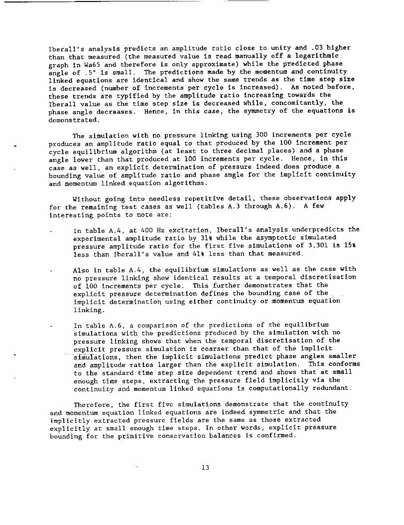
Iberall's analysis predicts an amplitude ratio close to unity and .03 higherthan that measured (the measured value is read manually off a logarithmic
graph in Wa65 and therefore is only approximate) while the predicted phase
angle of .5 ° is small. The predictions made by the momentum and continuity
linked equations are identical and show the same trends as the time step size
is decreased (number of increments per cycle is increased). As noted before,
these trends are typified by the amplitude ratio increasing towards the
Iberall value as the time step size is decreased while, concomitantly, the
phase angle decreases. Hence, in this case, the symmetry of the equations is
demonstrated.
The simulation with no pressure linking using 300 increments per cycle
produces an amplitude ratio equal to that produced by the i00 increment per
cycle equilibrium algorithm (at least to three decimal places) and a phase
angle lower than that produced at i00 increments per cycle. Hence, in this
case as well, an explicit determination of pressure indeed does produce a
bounding value of amplitude ratio and phase angle for the implicit continuity
and momentum linked equation algorithms.
Without going into needless repetitive detail, these observations apply
for the remaining test cases as well (tables A.3 through A,6). A few
interesting points to note are:
In table A.4, at 400 Hz excitation, Iberall's analysis underpredicts the
experimental amplitude ratio by 31% while the asymptotic simulated
pressure amplitude ratio for the first five simulations of 3.301 is 15%
less than Iberall's value and 41% less than that measured.
Also in table A.4, the equilibrium simulations as well as the case with
no pressure linking show identical results at a temporal discretisation
of I00 increments per cycle. This further demonstrates that the
explicit pressure determination defines the bounding case of the
implicit determinatio_ using either continuity or momentum equation
linking.
In table A.6, a comparison of the predictions of the equilibrium
simulations with the predictions produced by the simulation with no
pressure linking shows that when the temporal discretisation of the
explicit pressure simulation is coarser than that of the implicit
simulations, then the implicit simulations predict phase angles smaller
and amplitude ratios larger than the explicit simulation. This conforms
to the standard time step size dependent trend and shows that at small
enough time steps, extracting the pressure field implicitly via the
continuity and momentum linked equations is computationally redundant.
Therefore, the first five simulations demonstrate that the continuity
and momentum equation linked equations are indeed symmetric and that the
implicitly extracted pressure fields are the same as those extracted
explicitly at small enough time steps. In other words, explicit pressure
bounding for the primitive conservation balances is confirmed.
13

Consequently, the remaining n - step implicit simulations were carried
out using the momentum linked formulation as it is numerically more efficient
than its symmetrical continuity or pressure-linked counterpart because one
less matrix inversion is required for each iteration.
Reverting to table A.2, it may be observed that the UPD and
characteristically determined time step versions (numbers 6 and 8) produce
identical results in terms of amplitude ratio versus increments per time step.
The trend in both cases conforms to the standard pattern, namely, amplitude
ratio increasing with decreasing sub-time step size. Furthermore, the
amplitude ratio at 13 increments per time steps conforms to the limiting value
produced by the single step implicit simulations (numbers 3 and 4). In terms
of phase angle behavior, the UPD and characteristic versions of the n - step
implicit algorithm show the same trend (phase angle decreasing with increasing
number of increments) except that there is some disparity between the
numerical values. This is caused by the relative lack of cyclic convergence
of the characteristic version (cyclic energy balance errors > 1% versus
equivalent errors for the UPD version < .01%). The characteristic version
takes an inordinately large number of cycles to reach cyclic equilibrium and
hence the simulation was terminated before full convergence was achieved as a
matter of expediency. Hence the characteristic version, while being a useful
test of numerical algorithm independence, is not a practical methodology.
Finally, the behavior of the n - step globally implicit algorithm shown
in table A.2 is rather interesting. A discretisation of 20 increments per
cycle proved to be the largest practical value that would enable the
coefficient matrices to be inverted (using a computer with a 64 bit precision
word length) before numerical round-off errors caused the simulation to become
unstable. This situation could be alleviated somewhat by various
normalization schemes as well as by matrix partitioning algorithms. However,
in the context of this investigation, such endeavors would not add materially
to the outcome and hence were not attempted. In this context, the n - step
globally implicit scheme conforms to the established pattern of amplitude
ratio and phase angle behavior observed for all the other simulations.
Examining the phase angle behavior, one is tempted to infer that the value
asymptotes to the Iberall value of .525 ° However, in temporal discretisation
terms, at 20 increments per cycle, the algorithm is in the range of the UPD
algorithm, which with Nch = 22.864 yields a temporal dfscretisation of 23
increments per cycle. Thus at 20 increments per cycle, the n - step globally
implicit algorithm produces a phase angle greater than the 23 increment per
cycle UPD algorithm which is in conformity with the established trend.
With minor variations, these observations also apply to the results
produced by the n step implicit simulations for all the remaining test cases
in tables A.3 through A.6. The only exceptions worth noting occur in tables
A.4 and A.6 in which the phase angle produced by the globally implicit
simulation at i0 increments per cycle is greater than that produced at 5
increments per cycle. Once again, these exceptions are caused by cyclic
equilibrium convergence effects where the particular simulations are not as
converged as their counterparts. However, since the phase angles in all cases
at 20 increments per cycle are less than those at coarser discretisations, thebasic behavioral trend is not violated.
14

Therefore, the n - step globally implicit simulations confirm that the
simulation predictions are independent of the particular form of the
integration algorithm used to solve the conservation balances. Furthermore,
use of an n step implicit algorithm does not appear to offer any numerical
accuracy advantages that cannot be achieved at a lower computational cost
using a single step implicit Crank-Nicholson algorithm with a finer temporal
dlscretisation. In this vein, there does not appear to be any advantage in
using a globally implicit algorithm, at least in terms of a strict transient
simulation.
15
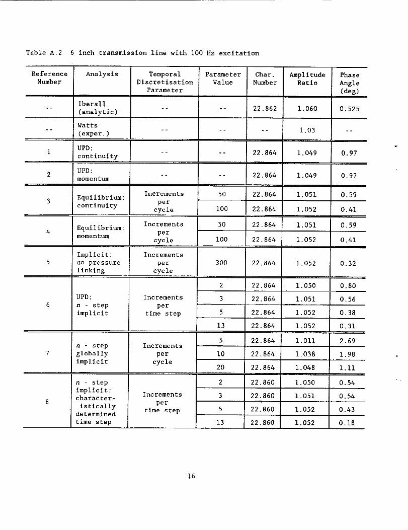
Table A.2 6 inch transmission line with I00 Hz excitation
ReferenceNumber
Analysis
Iberall(analytic)
Watts(exper.)
UPD:continuity
UPD:momentum
Equilibrium:continuity
Equilibrium:momentum
Implicit:no pressurelinking
UPD:n - step
implicit
n - step
globally
implicit
n step
implicit:character-
isticallydetermined
time step
TemporalDiscretisation
Parameter
Increments
per
cycle
Increments
per
cycle,,,.,,._.......... , ,, ,
Increments
per
cycle
Increments
per
time step
Increments
per
cycle
Increments
per
time step
Parameter
Value
, . ,T
50
I00
Char.
Number
22.862
22.864
22,864
22.864
22.864
50 22.864
i00 22.864
300 22.864
13
22.864
22.864
22.864
22.864
5 22.864
I0 22.864
20 22.864
2 22.860
3
AmplitudeRatio
1.060
1.03
,,,, ,,
i.049
I. 049
Phase
Angle
(deg)
0.525
0.97
0.97
1.051 0.59
1.052 0.41
1.051 0.59
1.052 0.41
1.052
1.050
0.32
0.80
1.051 0.56
1.052 0.38
1.052
1.011
I. 050
0,31
2.69
1.038 1.98
1.048 I.II.,.,,,-
O. 54
22.860 1.051 0.54
5 22.860 1.052 0.43
13 22.860 0.181.052
16
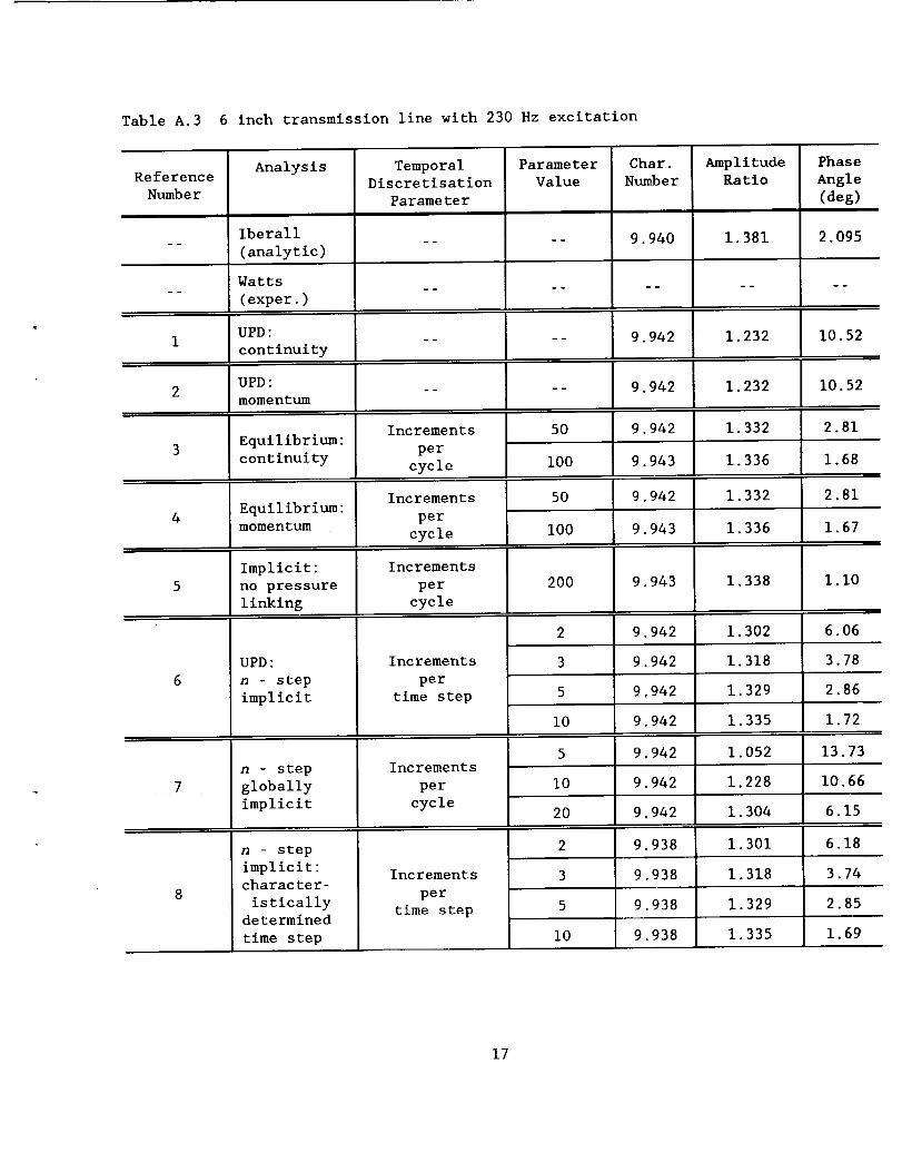
Table A.3 6 inch transmission line with 230 Hz excitation
Reference
Number
Analysis
Iberall
(analytic)
Watts
(exper.)
TemporalDiscretisation
Parameter
Parameter
Value
Char.
Number
9. 940
AmplitudeRatio
1.381
UPD:i .... 9.942 1.232
continuity
UPD:2 .... 9.942 1.232
momentum
50 9.942 1.3323 Equilibrium:
continuity i00
5O
4 Equil ibr ium-
momentum
9.943
9.942
Increments
per
cycle
Increments
per
cycle
1.336
1.332
Phase
Angle
(deg)
2.095
10.52
10.52
2.81
1.68
2.81
i00 9.943 1.336 1.67
Implicit: Increments
5 no pressure per 200 9.943 1.338 I.I0
linking cycle
2 9.942 1.302 6.06
6
UPD:
n step
implicit
Increments
per
time step
Increments
per
cycle
3 9.942 1.318
5 9.942 1.329
1.335i0
i0
Increments
per
time step
n step
globally
implicit
n - step
implicit"character-
isticallydetermined
time step
7
20
9. 942
9.942 1.052
9.942 1.228
9.942 1.304
2 9.938 1.301
3 9.938 1.318
5 9.938 1.329
9.938I0 1.335
3.78
2.86
1.72
13.73
10.66
6.15
6.18
3.74
2.85
1.69
17

Table A.4 6 inch transmission line with 400 Hz excitation
ReferenceNumber
Analysis TemporalDiscretisation
Parameter
ParameterValue
UPD:continuity
Char.Number
AmplitudeRatio
PhaseAngle(deg)
, , , ,,
.- Iberall .... 5.716 3.885 10.886(analytic)
__ Watts ...... 5.6 --(exper.)
i .... 5.718 1.208 40.12
UPD:
momentum,l
Equilibrium:
continuity
Equil ibr ium :
momentum
3
Increments
per
cycle
Increments
per
cycle
Increments
per
cycle
Increments
per
time step
Increments
per
cycle
Increments
per
time step
Implicit"
no pressure
linking
5O
I00
50
i00
5.718 1.209 40.18
5.721
5.721
5.720
5.721
UPD:
n - step
implicit
i00 5.721
17
3.180
3. 301
3.180
3.301
3.301
15.86
9.04
n - step
globally
implicit
15.85
9.03
2 5.719 1.997
3 5.720 2.470
9 5.721 3.171 14.76
5.721 3.285 8.96
9.07
39.2!
32.55
5 5.717 1.029 38.78
I0 5.718 1.791 42.70
20 5.720 31.522.604
1.972
2.412
3.123
3.281
n - step
implicit:character-
istically
determined
time step 17
5.712
5.712
5,711
5.711
38.84
34.08
19.48
14.80
18

Table A.5 24 inch transmission line with 55 Hz excitation
Reference
Number
I
2
3
4
5
Analysis
Iberall
(analytic)
Watts
(exper.)
UPD:
continuity
UPD:
momentum
Equilibrlum:
continuity
Equilibrium:
momentum
Implicit:
no pressure
linking
UPD:
n step
implicit
n step
globally
implicit
n - step
implicit:character-
istically
determined
time step
TemporalDiscretisation
Parameter
Increments
per
cycle
Increments
per
cycle
Increments
per
cycle
Increments
per
time step
Increments
per
cycle
Increments
per
time step
Parameter
Value
50
i00
50
i00
170
2
3
5
I0
5
i0
20
Char.
Number
10.340
Amplitude
Ratio
1.299
Phase
Angle
(deg)
3. 607
10.341 1.162 8.62
10.341 1.162 8.62
10.341 1.234 3.22
10.341 1.237 2.50
10.341 1.234 3.23
10.341 1.237 2.50
10.341 1.238 2.23
10.341 1.214 5.47
10.341 1.226 4.03
1.233
1.237
10.341
I0. 341
3.32
2.53
10.341 1.032 11.30
10.341 1.161 8.68
10.341 1.214 5.50
2 10.338 1.215 5.16
3 10.338 1.226 4.25
5 10.338 1.234 3.50
10.338 1.238 2.84i0
19

Table A.6 24 inch transmission line with II0 Hz excitation
ReferenceNumber
Analysis
Iberall(analytic)
Watts(exper.)
TemporalDiscretisation
Parameter
ParameterValue
Char.Number
5.170
AmplitudeRatio
4.252
UPD:i .... 5.171 1.008continuity
UPD:2 .... 5.171momentum
Equilibrium:continuity
50
100
50Equilibrium:momentum
4
5. 174
5.174
5.174
Increments
per
cycle
Increments
per
cycle
1.008
3.070
3.209
3.070
Phase
Angle
(deg)
25.419
40.10
40. ii
19.60
13.26
19.60
i00 5.174 3.209
Implicit: Increments
5 no pressure per 90 5.174 3.196 13.99
linking cycle
2 43.62
13.26
5.172 1.743,, ,, ,
3 5.173 2.211 38.82
I0 5.174 3.063 19.55
20 5.174 3.204 13.30
5 5.171
UPD:
n - step
implicit
n step
globally
implicit
1.007 39.91
i0 5.172 1.743 43.97
20 5.173 2.512 33.88
2 5.167 1.798 42.56
5.167
5.166
2.262
3.069
2.942
Increments
per
time step
i0...... J
Increments
per
cycle
Increments
per
time step
n step
implicit:character-
istically
determined
time step
6
2O 5.166
37.81
19.14
16.79
20
A.7 CONCLUSION
The results confirm that the discretised primitive integral conservation
balances have the following features:
they are mathematically symmetrical with respect to continuity and
momentum equation linking.
- when they are solved implicitly, as the time increment is decreased, the
pressure field solution obtained using either a continuity or momentum
linked equation set approaches the solution obtained explicitly from the
continuity equation via an equation of state.
- in terms of the transmission line, their solution is independent of the
form of the implicit numerical integration algorithm used.
Therefore, in the light of these confirmations, it seems reasonable to
conclude that the discretised pressure or mass flux linked primitive
conservation balances used in the simulations are not unconditionally valid
for modelling transmission line information propagation effects at
characteristic numbers less than about 24. To the extent that these specific
effects are also present in Stirling machines (in particular, the SPDE and
SPRE), it is consistent to infer that Stirling machine simulations based on
these primitive conservation balances are also open to question.
In particular, at low characteristic numbers, neither the pressure-
linked nor mass-linked formulations appear to replicate the physical behavior
described by the Kirchoff momentum equation or by the wave equation, despite
attempts to impose a characteristics solution on the pressure-linked
formulation using either a UPD or a characteristically determined, variable
time step hypothesis.
This position is supported by Iberall's analysis itself, by the results
of Organ's linear wave equation approach (OJ89) as well as by MacCormack's
analysis (Mc82),
21

PART
ENTROPY TRA_S_0RT
I
B. 1 INTRODUCTION
The investigation of entropy transport resolved itself into two tasks.
In the first task, a previously developed suite of codes used for simulating
the Mechanical Engineering Test Rig (METR) (Go90) was applied to Kurzweg's
apparatus and validated against his experimental and closed-form analytic
data. Thereafter, an entropy transport equation was developed and evaluated
in the validated codes. These activities may be resolved into the following
specific tasks:
a. The adaptation of the Mechanical Engineering Test Rig (METR) one- and
two-dlmenslonal codes (Go90) to Kurzweg's enhanced diffusion oscillating
flow test apparatus (KZ84).
b.
The formulation of an entropy postulate and its rigorous transformation
into an entropy transport equation to be tested in a code applied to
Kurzweg's apparatus.
B.2 INITIAL OBSERVATIONS
Kurzweg's apparatus is based on incompressible (water) fluid flow.
However, in view of NASA's interest in the compressible oscillating flows
occurring in Stirling cycle machines, it was originally intended to simulate
Kurzweg's apparatus using a compressible fluid. This was also logistically
prudent since the METR codes are strictly appropriate for compressible flows.
However, early on during task a it became clear that the original intention of
using a compressible fluid was not feasible for at least the followingreasons:
reference KZ84 provides insufficient geometrical detail about the
variable volume cavities at either end of the capillary tube bundle to
enable the compressible flow boundary conditions to be specified
completely.
in order to remain within the laminar flow regime specified for the
applicability of the analysis described in KZ84, very small compressible
flow oscillation frequencies and tidal displacements are required. Under
these conditions, other effects not accounted for by Kurzweg (such as
buoyancy effects) may be expected to influence the results. In this
case, the validity of the experimental data in KZ84 under compressible
flow conditions is questionable.
22

Thus it was decided to enhancethe METR codes to describe incompressible
flows also so that they could be applied directly to Kurweg's apparatus
without the above two limitations ....
Initial validation efforts with the two-dimensional code at the chosen
test point (see section B.3), consistently yielded effective diffusivities
four to five times larger than those measured or predicted analytically. The
simulation was found to be very sensitive to axial discretisation so that each
decrease in discrete volume axial length decreased the simulated effective
diffusivity, edging it ever closer to the nominal experimental value. At a
discretisation of i discrete volume per millimeter, the overprediction had
been reduced to a factor of 2 at the expense of a very large increase in
computational effort, almost overwhelming the computer equipment available for
the project.
These observations are prima facie evidence of the ubiquitous "false
diffusion" problem that plagues numerical analysis in general and integral
analysis in particular. Hence further progress mandated the development of an
algorithm for eliminating the false diffusion problem inherent in the
discretised integral description of the continuum mechanics used in the
simulation. This made inclusion of entropy transport in the simulations of
vital importance, since false diffusion correction schemes do have the
potential for violating the second law of thermodynamics.
In order to develop such a false diffusion correction algorithm, it was
judged prudent to do the development work using a one-dimensional simulation
of Kurzweg's apparatus rather than a twoldimgnsional code since this was felt
to be more time-effective in the long run. Furthermore, since the one-
dimensional simulation uses the standard Kays and London (KL64) steady-state
heat transfer coefficient and friction factor correlations, such a simulation
provides another experimentally based test point for evaluating the accuracy
of such correlations in describing oscillating flows.
B.3 TEST CONDITIONS
The test apparatus simulated is shown in figure B.I. Essentially, the
device consists of an upper and a lower cavity joined by an acrylic tube
containing a bundle of glass tubes. These tubes apparently are not fitted_
into a manifold ateither end so that the Dgt flow area consists of the
internal tube areas as well as the triangular areas between the tubes (figure
B.2). The external axial faces of the hot and cold reservoirs are fitted with
flexible membranes so that when the entiK_ apparatus is oscillated by a
shaker, the fluid (water) will undergo corresponding oscillations. Finally,
the apparatus is cocooned in insulation so maintaining a nominally adiabatic
boundary with the surroundings.
23
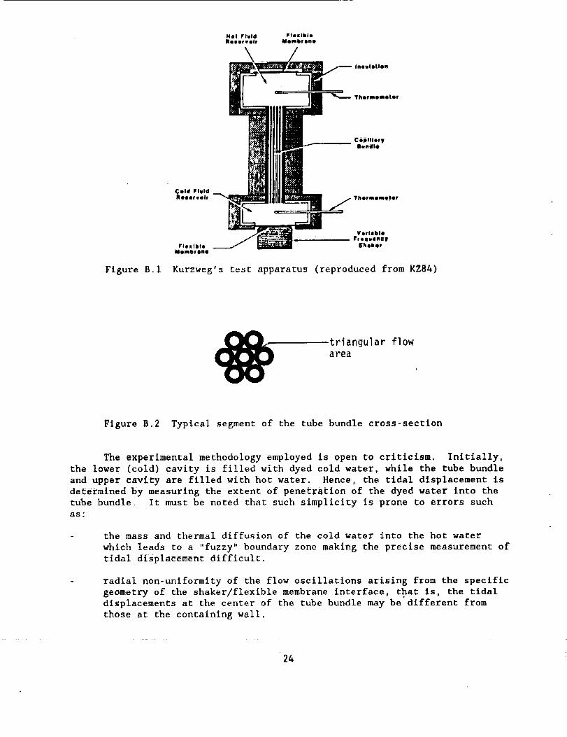
Hot Fluid FluxlbloNeeorvolr Mombrono
Figure B.I
Fie nlbloMombfJnQ
InoullLlen
YhoJ, moNtqJtof
CuJllllofyIlundie
Thormomotor
VorlebJd
FrequdnclP8hokor
Kurzweg's test apparatus (reproduced from KZ84)
triangular flow
a rea
Figure B.2 Typical segment of the tube bundle cross-section
The experimental methodology employed is open to criticism. Initially,
the lower (cold) cavity is filled with dyed cold water, while the tube bundle
and upper cavity are filled with hot water• Hence, the tidal displacement is
determined by measuring the extent of penetration of the dyed water into the
tube bundle, it must be noted that such simplicity is prone to errors such
as:
the mass and thermal diffusion of the cold water into the hot water
which leads to a "fuzzy" boundary zone making the precise measurement of
tidal displacement difficult.
radial non-uniformity of the flow oscillations arising from the specific
geometry of the shaker/flexible membrane interface, that is, the tidal
displacements at the center of the tube bundle may be different from
those at the containing wall.
24

surface tension effects within the capillaries which would complicate
the external measurement of the mid-meniscus position.
Kurzweg and Zhao do not appear to acknowledge these problems in the
light of the good agreement they obtain (in logarithmic terms) between their
analytic and experimental results (KZ84, figure 2). However, since they use a
data fitting approach to obtaining this agreement (by adjusting the Prandtl
number via the choice of system temperature), it is reasonable to suppose that
many of the systematic errors which would degrade this good agreement are
buried in the data fitting process.
The upper and lower cavity temperatures are measured via thermometers
read at one minute intervals for a total experimental run time of 6 minutes.
The heat flowing through the tube and resuitant effective diffuslvity are
determined exclusively from these measurements. In particular, the resulting
inferred temporal temperature gradient of the cold cavity (from which the net
heat flowing down the tube is computed)_'iS highly approximate in comparison
with the instantaneous axial temperature gradient used in the effective
diffusivity calculation (KZ84, equation I) (a time-averaged axial temperature
gradient would have been more appropriate). Hence this additional source of
systematic error is also embedded in the Prandtl number data fit.
Needless to say, these issues complicate the simulation, particularly
when the objective is to obtain agreement with the experimental and
"validated" analytic results. However, of perhaps even more importance from a
simulation perspective, is the difficulty of simulating the initial
discontinuous (literally "brick wall") temperature profile at the tube bundle
/ cold cavity interface. Such a condition has been documented in the
literature (for example, BB75) to magnify the effects of false diffusion in
producing erroneous advective fluxes.
Hence within these limitations, the following simulation approach is
adopted
a. All the available physical parameters describing the apparatus and test
conditions given in KZ84 are used as described in table B.I.
b, The three additional geometrical parameters needed to implement the
simulation were determined by direct measurement of figure B.I in the
hope that the relative scale of the figure is somewhat representative of
reality. These parameters are:
Hot/cold cavity cross-sectional area ratio = i
Stationary hot/cold cavity length ratio = 1.714
Cold cavity / casing cross sectional area ratio _ 4 8
Fortunately, under incompressible flow conditions, errors in these
ratios do not effect the flow within the tube bundle provide4 mass flux
boundary conditions are used. They do have an effect when pressure
boundary conditions are invoked.
25
ORIGINAL PAGE IS
OF POOR QUALITY
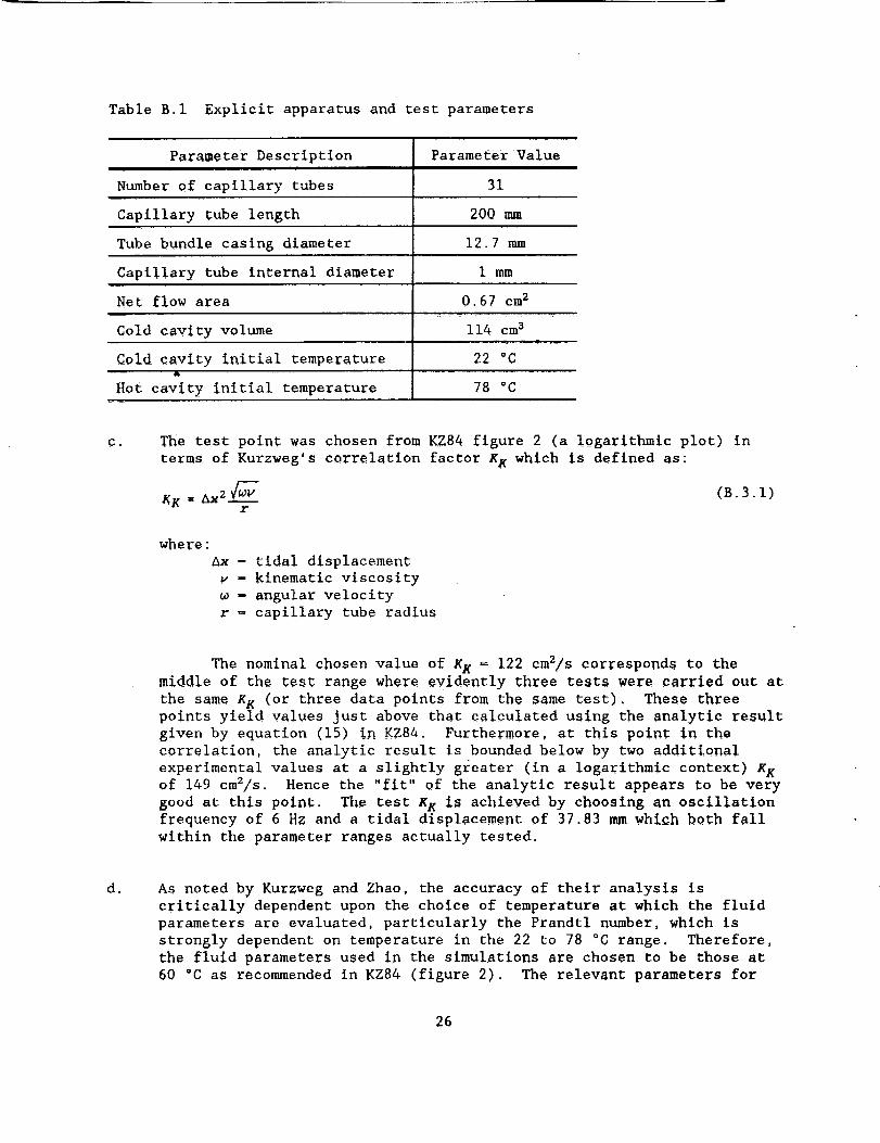
Table B.I Explicit apparatus and test parameters
Parameter Description
Number of capillary tubes
Parameter Value
31
Capillary tube length 200 mm
Tube bundle casing diameter 12.7 mm
Capillary tube internal diameter I mm
Net flow area 0.67 cm 2
Cold cavity volume 114 cm 3
Gold cavity initial temperature 22 °C
Hot cavity initial temperature 78 °C
C. The test point was chosen from KZ84 figure 2 (a logarithmic plot) in
terms of Eurzweg's correlation factor KK which is defined as:
= _2_ (B.3 i)KK .....r
where:
Ax = tidal displacement
w = kinematic viscosity
- angular velocity
r - capillary tube radius
The nominal chosen value of KK = 122 cm2/s corresponds to the
middle of the test range where evidently three tests were carried out at
the same KK (or three data points from the same test). These three
points yield values Just above that calculated using the analytic result
given by equation (15) in KZ84. Furthermore, at this point in the
correlation, the analytic result is bounded below by two additional
experimental values at a slightly greater (in a IQgarithmic context) KK
of 149 cmZ/s. Hence the "fit" of the analytic result appears to be very
good at this point. The test KK is achieved by choosing an oscillation
frequency of 6 Hz and a tidal displacement of 37.83 mm whiGh both fall
within the parameter ranges actually tested.
d. As noted by Kurzweg and Zhao, the accuracy of their analysis is
critically dependent upon the choice of temperature at which the fluid
parameters are evaluated, particularly the Prandtl number, which is
strongly dependent on temperature in the 22 to 78 °C range. Therefore,
the fluid parameters used in the simulations are chosen to be those at
60 °C as recommended in KZ84 (figure 2). The relevant parameters for
26

water at this temperature together with those of glass (necessary formodelling the capillary tube walls) are given in table B.2.
Table B.2 Fluid and wall material properties
Property Water (Sc79) Glass (ASH81)i
Density (kg/m 3) ' 983.3 2470
Specific heat capacity (J/kg.K) 4191 750
Thermal conductivity (W/m.K) 0.65 1.0
Dynamic viscosity (kg/m.s) 47.0 x 10 -5 --
Prandtl number 3.01 --
e.
It must be pointed out that a better approach would be to include these
parameters in the simulation as temperature dependent entities.
However, in the interest of reducing the differences between the
simulation and the analysis (the major objective being to use the
analysis as fitted to the experimental data as the validation standard),
it was decided to proceed on the above basis.
The method used to calculate the effective diffusivity in the simulation
corresponds to that of KZ84 and is given by:
I_ Vc dT c_eff = ube (rh- rc)--_(B.3.2)
In applying equation (B.3.2), the rate of temperature change in the cold
cavity is computed as the net cyclic temperature change rate, that is,
the difference between the cold cavity temperatures at the end and
beginning of a cycle divided by the period. This enables the change in
effective diffuslvity to be tracked as a function of time so that the
simulation can be terminated as soon as the rate of change of the
simulated effective diffusivity becomes small. Ultimately, of course,
the effective diffuslvity becomes infinite when the hot and cold
cavities reach thermal equilibrium. This achieves the same physical
purpose as Kurzweg's experimental procedure while minimizing the amount
of computation. In practice, a simulation period of .5 minutes proved
more than adequate under these conditions.
B.4 THE FALSE DIFFUSION CORRECTION METHODOLOGY
False diffusion arises in transient continuum mechanics numerical
analysis in the discretisation of the advection terms in the conservation
balances. Typically, when using any variation of upwind difference or upwind
parameter methodology (whether the second upwind difference formulation of
27

Gentry, Martin and Daly (GM66) or the equilibrium analytic approach of
Patankar (Pa80))$ the advected flux on the Control volume boundary is biased
towards the upwind advected parameter rather than the actual value of the
parameter at the boundary. In general, the actual value of the advected
parameter is different from both the upwind and downwind va!ues in a
continuous system. In Stirling machine analysis, false diffusion is known to
be a significant cause of error in modelling the working fluid in the
regenerator (originally pointed out by Gedeon (Ge84)).
The literature on false diffusion is quite voluminous as it long has
been recognized as one of the principal difficulties in numerical analysis.
However, most of the algorithms developed for correcting or eliminating false
diffusion are based on discretisations of the differential conservation
balances, particular examples being the SHASTA algorithm of Book, Boris and
Hain (BB75) and the sequential backward difference predictor / forward
difference corrector methodology of MacCormack (Mc82). Unfortunately, none of
these schemes works well in an integral environment where there are no
parameter gradients to be exploited in the advection terms.
The first attempt made was to invoke the upwind linear extrapolation
method successfully used in Go87 for modelling false diffusion in the
regenerator of Stifling machines. Theoretically, such an approach could be
expected to work well in simulating Kurzweg's apparatus, since in time, the
temperature profile between the hot and cold cavities becomes linear.
However, at startup, in the presence of the discontinuous temperature gradient
at the cold cavity entrance, the method fails badly, and later, even under
milder temperature gradient conditions, the method yields an over-predictlon
of the effective diffusivity.
Hence, after much analysis and computation, an apparently effective and
unconditionally stable false diffuslon correction methodology was developed.
The methodology may be described in terms of the following generalized
algorithmic sequence:
a, Pre4ict the parameter field _" using a conventional second upwind
difference spatial discretisation (Go87). In general, an explicit,
implicit or hybrid integration scheme may be used for this step.
b. Calculate the source term from:
28
;_. • • (s.4.1)Ksource = (¢.w-_n) (gn'") dA
C0
where:
@uw = #i-i if gni _ 0
_uw = @i if gni < 0
It may be noted that no restrictions need be placed on the form of the
interpolating function f provided it is bounded symmetrically, for
example, f may be a polynomial of odd order.
The correction field A# is found implicitly from:
MA_At = _ _uw(-gn'-n)dA+KsOurce(B.4.2)
where:
A@u w = d_i_ 1 if -gni _ 0
A@u w = A_i if -gni < 0
d. Calculate the corrected parameter field _ given by:
= _'+_(B.4.3)
e. Iterate from step a until the change in the corrected parameter field
becomes appropriately small.
In practice, the iteration required in step e does not add to the
iterations required in any case to implement the pressure or non-pressure
linked algorithms discussed in part A. Two interpolating functions have been
tested for use in step b, namely linear and cubic polynomials. As shown by
the results (section B.7), both schemes produce almost the same results,
however, during the transient start-up phase, the cubic function yields a
better approximation of the temperature field at the cold cavity entrance.
A negative consequence of the false diffusion correction algorithm
described above is that it necessitates one more matrix inversion per
conservation equation per iteration. However, in terms of an integral
analysis, this is more than offset by at least a six-fold reduction in the
required discreti_ation combined with better accuracy at the coarser
discretisation than obtained using the upwind approach alone at the finer
discretisation. In this context, it must be pointed out that the flux
correction methodology developed is still embryonic and is capable of much
enhancement.
29

B.5 P_VE_OPMENT OF AN _NT_OPY TRANSPORT EQUATION
The approach adopted in deriving the entropy transport equation is
ideDtlcal in nature to that documented in Go87 for the mass, momentum and
energy balances. The essential difficulty (at least philosophically) is in
defining an appropriate entropy postu!ate. One traditional approach is to
define entropy as being that which requires thermodynamic processes to be
unidirectional, for example, according to Wark (Wa77):
"Any system having certain specified constraints and having an
upper bpund in volume can reach from any initial state a stable
equilibrium state with no net effect on the environment."
The corollary to this postulate, known as the Kelvin-Planck statement (Wa77),
is sufficient to allow proof of C!auslus' inequality as a theorem, that is for
a closed system:
which in turn allows the "increase in entropy" principle to be derived, or_
d_ .6_ (B. 5.2)
where E denotes entropy.
Equation (B.5.2) is invoked by some authors directly as an entropic
postulat!onal basis, for instance Slattery's entropy postulate (S181) that:
"The minimum rate of production of entropy in a body is
proportional to the rate of energy transmission to the body."
or symbolically:
: (B.5.3)
where the terms on the RHS represent the entropy changes produced by contact
energy transmission to the body through its bounding surface and by external
and mutual energy transmission respectively.
However, from a computational point of view, neither of these postulates
is determinate, that is, they do not allow entropy to be definitely
calculated. Hence for this reason, the following entropy postulate based on a
statement originally proposed by Truesdell and Toupin (TT60) as the basic
assumption of thermodynamics is preferred:
30

Postulate V A dimensionally independent scalar parameter _ (termed specific
entropy) and the substate densities are sufficient to determine
the specific internal energy of a material particle independently
of time, place, motion and stress.
That is :
(B.5.4)
This postulate is not equivalent to those quoted above in the sense that
it is not based upon a manifestation of entropy, but rather is an equation of
state for internal energy which requires that entropy be a fundamental
property. However, the consequences of equation (B.5.4) must satisfy the
previous conventional postulates as expressed in a general fashion by equation
(B.5.3).
When a particular body is thermodynamically homogeneous, that is every
particle p is behaviorally identical, equation (B.5.4) may be simplified to:
0= 0_,V, Fi) (B.5.5)
where F is the mass (or mole) fraction of species i. In terms of the single
component working fluids being considered here (and hence also for Stirling
machines in most cases), it is useful for the sake of simplicity to proceed by
considering single specie entities only, that is:
= 0(_,#) (B.5.6)
dU = Td_--PdV(B.5.7)
Taking the substantive derivative, multiplying through by p, substituting Go87
equation (C.7) (which relates the change in size of a discrete volume to the
motion of its enclosing boundaries) and simplifying:
PD-{ = p2 -P(V.v) (B.5.8)
The substantive differential energy balance at every point in a material body
is given by (Go87):
DU = pE + (T:Vv) -P(V.v) -V._"P-D--_
(B.5.9)
31

Equating (B.5.8) and (B.5.9), expanding and rearranging:
+ -v.- wp_ (r:Vv) (B.5.10)
P = T z z
Integrating (B.5.10) over the material body volume V(m ) and substituting Go87
equations (C.9) and (C.10) yields after simplification and rearrangement:
= + - + ( -.)dAd _V(.oP'_" dV ;V(,,,) T(B.5.11)
Rearranging the right hand side:
P_ dV+ _ i (T-Vw) }-aT(B.5.12)
Comparing equations (B.5.12) and (B.5.3) and noting that the last
integral on the RHS of (B.5.12) is strictly positive (because # = -kVT ),
reveals that the postulational basis of equation (B.5.4) indeed satisfies the
conventional entropy postulate as defined by equation (B.5.3) while
simultaneously being determinate.
Converting equation (B.5.10) into partial temporal derivative form and
substituting into the generalized transport equation (Go87, equation (C.12))
yields the final version of the entropy balance:
-c
"---6F'-- Jr(,)T[
+
(B.5.13)
In implementing the entropy transport equation, it was found that great
care must be taken in locating the entropy boundary (within which the cyclic
entropy is computed) and in describing the thermal transport across that
boundary. In this context, it should be noted that, by definition, the second
law of thermodynamics treats isolated systems so that Clausius' inequality
applies over the integral of the subsystems of which the isolated system is
comprised. In the limit, the only true isolated system is the entire
universe, so that extracting a computationally isolated system which can in
general exchange heat with its superordinate body is not obvious in all cases.
The approach adopted may be visualized in terms of figure B.3.
32

Y _/(An)isboundar isolated system
. gnJis(qn)is
Figure B.3 Isolating boundary entropy contribution
Consider a segment of the isolating boundary (An)is across which flows a mass
flux (gn)is and a thermal diffusion flux (_n)is The operating entroplc
principle governing the isolating boundary is:
The net contribution of the entropic and thermal fluxes crossing the
isolating boundary is assigned to the isolated system entropy
irrespective of the spatial location of these fluxes (which in general
span a part of the isolated system as well as the bounding environment).
Hence, applying equation (B.5.13) to the situation depicted in figure B.3
yields:
d CV]-'_-M d tV]=--M + _( -{(_n)isVTb}= [_Jinternal =V)b _ _ dV
(#nhsdA
(B.5.14)
where _ is an appropriate fraction for delineating the integration sub-volume
(typically _ - .5 for a conformal Cartesian mesh). It should be noted that
the advection entropy flux does not appear in equation (B.5.14) because its
net contribution to the isolated system entropy is zero.
The success in using the full entropy transport equation including
generalized isolated boundary heat transport may be judged from the results
presented in section B.7. As envisaged when proposing this study, Kurzweg's
laminar flow apparatus provides an ideal test bed for such an entropy
transport equation, since the transport Of entropy is clearly visible from a
system perspective and not compartmentalized between system components as
occurs; for example, in Stirling machines,
B.6 OTHER ISSUE S
During the process of testing the false diffusion correction algorithm,
it was found that careful attention had to be paid to modelling the conduction
heat transfer in the capillary tube walls. In particular, the effective
33

diffusivity was found to be sensitive to the manner in which the wall/fluld
interface is discretised, both in the capillary tubes as well as in the hot
and cold cavities. Although in the simulations (both one- and two-
dimensional) the capillary tube walls are modelled as axially discretised,
one-dimenslonal entities and this approach seems to yield good results, there
is a suspicion that a one-dlmenslonal approach is probably inadequate,
particularly at high radial heat transfer rates. Thus, in the future, thought
should be given to modelling Stirling heat exchanger walls as radially
dlscretised two-dlmenslonal entities to determine whether the above suspicion
has any basis.
Finally, as the results show, the limitations of a first order temporal
integration scheme became manifest, particularly in the two-dimensional
simulation. However, owing to time constraints, the first order temporal
integration algorithm in the METR two-dimensional code could not be upgraded
to second order (a second order one-dimensional code had been developed and
tested previously (Go90)).
B.7 RESULTS
The results of all the simulations undertaken are summarized in table
B.3. At the chosen test point, the effective dlffuslvity produced by
Kurzweg's analysis amounts to 4.8 cmZ/s with the corresponding experimental
values ranging between 5.8 and 7.4 cmZ/s. Using an axial discretisation of 30
discrete volumes (.15 discrete volumes per millimeter) and a temporal
discretisation of i00 increments per_cycle, the first order one-dimensional
simulation with no false diffusion correction over-predicted the effective
diffusivity by a range of 2.9 to 4.4 times (corresponding to the upper
experimental and analytic values respectively). As noted above, including the
false diffusion correction produced a simulated value for effective
diffusivity within the experimental range and at most 36% greater than that
analytically predicted, In contrast, upgrading the one-dimensional simulation
t0 Second order £emporal accuracy, reduced the over-prediction of effective
diffusivity with no correction to a range of 2.6 to 4.1 times. Including
either linear or cubic false diffusion correction produced a result within
3.5% of the analytic value.
Applying the second-order simulation at two other values of K K using
cubic false diffusion correction yields the results compiled in table B.4.
As discussed in section B.3 above, in view of the experimental
uncertainties, perhaps the "fitted" analytic value is indeed a reasonable
estimate of the actual effective diffusivity, in which case, discrepancies
less than 3.5% are an adequate validation of the false diffusion correction
methodology.
34
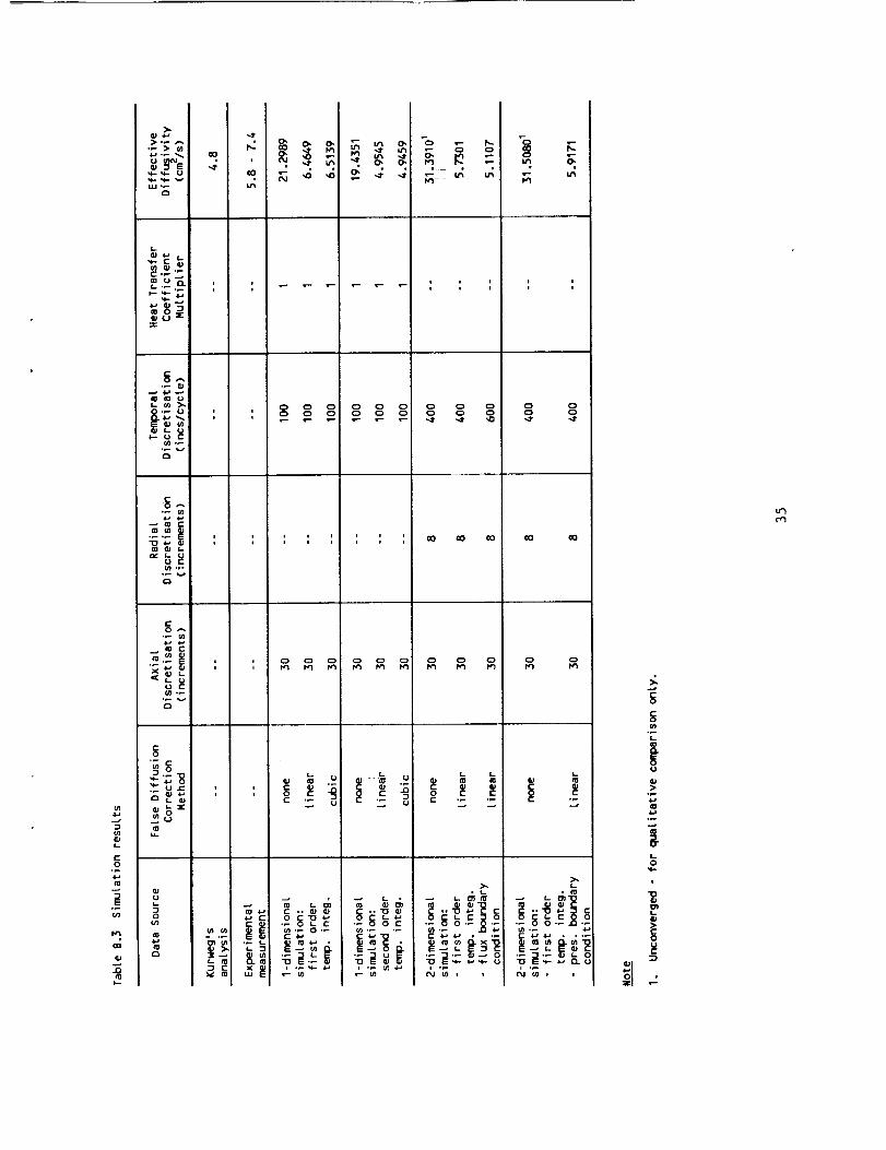
o_
°_
t- u _-
CO_
o
L_o t-
°_
o=
0 O
i i iQ ! l
c_ Q o
C_ 0 o
| i ui i l
o o
C_ c_
i i J
o 0 oC_ 0
CO O0 CO
Lt_
0t- ,_ ,p
00,4"
o
._ 0 0 t-
00
o
•" _- _
L
0

Table B.4 Effective diffusivity comparison
Correlation
Factor EE
(cmZls)
Effective Diffusivity (cmZ/s)
Kurzweg' s
Analysisi
4.8
Experimental
i
l-d Simulation
(cubic correction)
Analysis/Simulation
Discrepancy
(_)
122.0 5.8 7.4 4.9459 3.04
286.1 11.31 ii.i 11.0539 2.26
818.5 32.36 19.1 25.9 31.2692 3.37
However, of perhaps more interest, is the observation that all the one-
dimensional simulations were carried out using the nominal steady-state Kays
and London correlations without the necessity of any heat transfer coefficient
multipliers. For all these simulations, the Valensi number (square of the
Womers!ey number) is 19.7 which remains constant because it is independent of
tidal displacement. KK was varied in the simulations via the tidal
displacement while the frequency was kept constant at 6 Hz.
At a Valensi number of about 20, Uchida's analysis (UC56) of oscillating
laminar flows as quoted by Simon and Seume (SS86), yields amplitude
coefficients of pressure drop and wall shear stress of abou t 3.1 and 1.3
respectively. Also, at this Valensi number, Uchida's analysis predicts lead
phase angles of pressure drop and wall shear stress of approximately 68 ° and
28 ° respectively. Noting that for steady flow the amplitude coefficients are
unity and the lead phase angles are zero, it is evident that the simulations
represent a flow regime which is different from steady flow (particularly in
phase lead terms). Hence in view of the good agreement obtained in table B.4,
an argument can be made for the adequacy of the steady-state correlations for
predicting heat transfer under laminar oscillating flow conditions at Valensl
numbers less than 20 when the effects of false diffusion are minimized (if not
eliminated).
In developing the two-dimensional results, the importance of temporal
discretisation has already been alluded to. For this, reason, the hightemporal discretisations required to minimize the limitations of the first
order temporal integration algorithm used placed a severe load on the
available computing resources which constrained the number of runs carried out
to the half-minute closure point.
The axial discretisation was maintained at 30 discrete volumes while the
radial discre_isation could be comfortably limited to 8 discrete volumes.
With the false diffusion correction activated, increasing either of these
values produced a negligible change in the end result.
36

Hencein this context, other than tile temporal discretisation, the onlysignificant parameter was found to be the massflux boundary condition. Twoconditions were tested, namely:
specifying a radially uniform flow at the cold end tube entrance equalto the rate of change of the cold cavity volume.
using the rate of cold cavity volume change to generate a slnusoldallyvarying pressure which in turn allows the entrance mass fluxes to becalculated (a somewhatnebulous approach in the light of the paucity ofdata describing the hot and cold cavities).
In both cases, the hot cavity is treated as being isobaric atatmospheric pressure and gravity induced buoyancy forces are included in themomentumbalance.
In all cases, the uniform flux boundary condition produced slightlybetter results as might be expected. A shown in table B.3, only the linearfalse diffusion correction methodology was tested. At a temporaldiscretisation of 400 increments per cycle, the uniform flow boundarycondition simulation produced an effective diffusivity between theexperimental and analytic values, while increasing the discretisation to 600increments per cycle yields a simulated diffusivity 6.5%higher than theanalytic result and shows the diffusivity converging to the value predictedusing the second order one-dimensional code. Nevertheless, while yielding asatisfactory result, a discretisation of 600 increments per cycle is notpractical for an implicit code.
At the half minute cut-off, the false diffusion correction wasdeactivated with a resultant escalation of the effective diffusivity to anunconverged value in excess of 30 cm2/s. This is indicative qualitatively ofthe effectiveness of the false diffusion correction algorithm in twodimensions.
The results produced by the entropy transport equation are depicted infigures B.4 through B.9. Figure B.4 shows that the entropy is highest midwayalong the tube bundle and decreases towards both cavities. The hot cavityalways has a lower entropy than the cold cavity. Numerical output from thesimulation (not shown) confirms that the cyclic integral of the entropy overthe entire fluid system increases monotonically.
The cyclic temperature surface is depicted in figure B.5. Essentially,this shows a fairly invariant linear temperature profile flatteningalternately in the regions adjacent to the hot and cold cavities as the massflux reverses direction.
Combining figures B.4 and B.5 yields the temperature-specific entropy(T-E) diagrams of figures B.6 to B.9. Within the tube, figures B.7 and B.8show closed cycles whoseareas are exactly equal to the generated cyclicirreversibilities at those locations. As the tube acts as a thermal transferdevice between the hot and cold cavities and is externally adiabatic, closureof the T-E diagrams is thermodynamically necessary and thus an indication that
37

the entropy transport equation is operating correctly. All the entropygenerated in the tube is pumpedtowards the hot and cold cavities, both ofwhose entropies must increase monotonically which indeed is the case as shownin figures B.6 and B.9. In figure B.6, during the first part of the cyclewhen the flow is positive (that is, from the cold to the hot cavity), thespecific entropy increases marginally while the temperature drops (dissipationis not explicitly included in the cavities because of the absence of adequategeometrical data, see section B.3). Whenthe flow reverses, the entropygenerated in the capillary tubes is transported into the cold cavity soproducing the requisite monotonic cyclic entropy increase.
The inverse process occurs in the hot cavity as shown in figure B.9.During the first half of the cycle when the flow is positive, entropy istransported into the hot space while its temperature decreases. Notice thatover the cycle, the hot space has cooled while the cold space has becomewarmer.
At first sight, it may seemunreasonable that the temperature of thecold cavity decreases during positive flow and the hot cavity temperatureincreases during negative flow. However, bearing in mind that in an integralanalysis the reported temperatures are the volume-averaged temperatures andthat an axial temperature gradient exists through the cavities, then as massis removed from a cavity, its volume-averaged temperature must change. Hence,in the cold cavity, the removedfluid is hotter than the remaining fluid andhence the volume-averaged temperature decreases, with the inverse processoccurring in the hot cavity. This is a direct consequenceof the fluxcorrection methodology and reveals how it provides a more accurate descriptionof the continuum mechanics than the upwind difference approach. Inparticular, in the absenceof diffusion heat transfer from the ends of thecapillary tubes, the upwind algorithm yields constant temperatures in thecavities during their respective periods of massefflux.
38

Ld_
0 o
CI-.L- C_ o
0_.-
e--
D_I, _00 _--
_--_-_ 0
Z _o ._L_-- c
I
L_ ©
_N
L
C
00
E0L.
"(3
L--
0
E
0C0
e--
_Z3
0Z
39
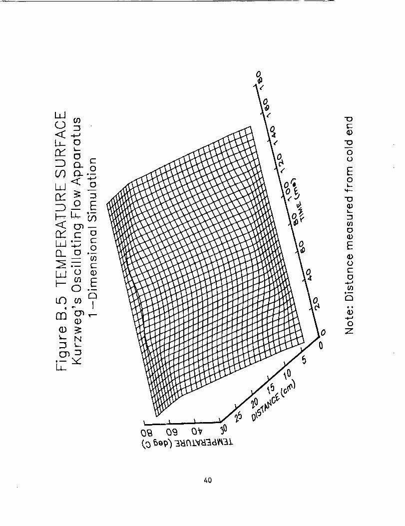
LdO0
l, o
LLJ 0
©
LL-
70C
7O
00
E0
70
@.._
@00
E
0C0
o_
n0 4
0Z
4O

o_
i |,
(),I'5)I/P)_kdO_LLN3 "03dS
i i i
(;H'O:M/P),kdO_l.l.N3"03dS
g
l.m.J
o
...I
0
-r
(TJ
,,r;
i i i | i
17 r- _ m
(>_-6,1/r)_,dO_±N:_"o3ds
o_
17I • I ¢ i & • •
u')
i,q
R
q)o
(>I'5:M/P),L_:IO_I.LN]"C)3=IS
41
B.8 CONCLUSION
The significant results obtained from the work carried out in part B,
have been the development of a tentatively effective false diffusion
correction methodology, its demonstration in one- and two-dlmensional
simulations and the development and evaluation of a rigorous entropy transport
equation. Using Kurzweg's oscillating flow apparatus as the target hardware,
in terms of the prevailing geometrical and experimental uncertainties, the
simulated data compare favorably with those generated analytically and
experimentally.
A comparison of the simulation and experimental/analytic data suggests
that under laminar, incompressible flow conditions at Valensi numbers less
than 20, standard steady-state heat transfer correlations are adequate for
predicting oscillating flow boundary heat transfers provided that the effects
of false diffusion are accounted for in the simulation.
Use of a fullLentropy transport equation in the simulation provides
useful physical insights into the irreversibility processes occurring within
oscillating flows.
The results produced should shed some additional light on the loss
mechanisms occurring within Stirllng cycle machines, at least in terms of
isolating possible sources of error in existing simulation design codes.
42

CLOSURE
The work carried out in part A suggests that the next logical steps for
investigating information propagation effects in Stirling machines might be:
the development and validation of a simulation based on a solution of
the full second order wave equation or Kirchoff momentum equation.
a transmission llne based investigation and validation of MacCormack's
characteristic factorlzation algorithm.
an experimental program to measure information propagation effects in
transmission lines and Stirling machines using precise digital acoustic
techniques. These tests should emphasize the accurate measurement of
phase angles in order to validate this aspect of Iberall's analysis as
well as to determine the information propagation characteristics of
actual Stirling hardware.
The results of part B suggest that the false diffusion correction
methodology developed may yield some improvement in the accuracy of existing
one-dimensional Stirling machine simulation codes. This improvement would
result from standard steady-state heat transfer correlations yielding better
accuracy while the enthalpy fluxes at the heater and cooler entrance and exit
ports also would be more accurately modelled.
Inclusion of entropy transport (as opposed to entropy generation alone)
in Stir!ing machine codes would yield a reliable method for tracking
irreversibilities within the engine and would allow a better comparison of the
performance of different simulation codes. Hence, as a next step, it seems
appropriate that the false diffusion correction algorithm and entropy
transport equation be ported to existing codes which should then be re-
validated against experimental data.
43
REFERENCES
ASHSl American Society of Heating, Refrigeration and Air-Condltioning
Engineers. Handbook of 1981 Fundamentals, ASHRAE, Atlanta, 1981.
BB75 Book, D.L., Boris, J.P. and Hain, K. 'Flux-Corrected Transport II:
Generalizations of the Method', Journal of Computational Physics, vol.
18, 1975, pp. 248-283.
Ge84
GM66
Gedeon, D. 'Numerical Advection Errors in Stirling Cycle Nodal
Analyses', Proceedings of the 19th IECEC, paper no. 849101, San
Francisco, 1984
Gentry, R.A., Martin, R.E. and Daly, B.J. 'An Eulerian Differencing
Method for Unsteady Compressible Flow Problems', Journal of
Computational Physics, vol. I, 1966, pp. 87-118.
Go68 Goldschmeid, F R. On the Dynamic Performance of Viscous Compressible
Fluids in Rigid Tubes with Volume Termination as a Function of Stokes
Number, NASA TM X-53785, 1968.
Go87 Goldberg, L.F. A State Space and Continuum Mechanics Analysis of
Stir!ing Cycle Machines, PhD Thesis, University of the Witwatersrand,
Johannesburg, 1987.
Gog0 Go!dberg, L.F. One- and Two-Dimensional Stirling Machine Simulation
Using Experimentally Generated Reversing Flow Turbulence Models, NASA
contractor report no. 185285, 1990.
Ib50 Iberall, A.S. Attenuation of Oscillatory Pressures in instrument Lines,
research paper RP2115, vol. 45, NBS, 1950.
Ji73 Jimenez, J. "Nonlinear gas oscillations in pipes. Part I. Theory",
Journal of Fluid Mechanics, vol. 59, part I, 1973, pp. 23-46.
KL64 Kays, W.M. and London, A.L. Compact Heat Exchangers, 2nd edition,
McGraw-Hill, New York, 1964.
Ko90 Kohler, W.J. Numerical Prediction of Turbulent Oscillating Flow and
Associated Heat Transfer, PhD Thesis, University of Minnesota,
Minneapolis, 1990.
KZ84 Kurzweg, U.H. and de Zhao, L. 'Heat transfer by high-frequency
oscillations: A new hydrodynamic technique for achieving large effective
thermal conductivities', Phys. Fluids, vol. 27, no. II, 1984, pp. 2624-
2627.
Mc82 MacCormack, R.W. "A Numerical Method for Solving the Equations of
Compressible Viscous Flow", AIAA Journal, vol. 20, no. 9, 1982, pp.
1275-1281.
44

0J89
Or82
PaSO
Ro82
St45
Sc79
SS86
TT60
Wa65
Wa77
Organ, A.J. and Jung, P.S. "The Stirling cycle as a linear wave
phenomenon", Proceedings IMechE, vol. 203, 1989, pp 301-309.
Organ, A.J. "Gas Dynamics of the temperature determined Stirllng
cycle", Journal of Mechanical Engineering Science, vol. 23, no. 4, 1982,
pp. 207-216.
Patankar, S.V. Numerical Heat Transfer and Fluid Flow, Hemisphere,
Washington D.C., 1980.
Roache, P.J. Computational Fluid Mechanics, Hermosa Publishers,
Albuquerque, 1982.
Strutt, J.W. (Lord Rayleigh) The Theory of Sound (Vol. If), 2nd
edition, Dover, New York, 1945.
Schlichtlng, H. Boundary-Layer Theory, 7th edition, McGraw-Hill, New
York, 1979.
Seume, J. and Simon, T. 'Oscillating Flow in Stirling Engine Heat
Exchangers', Proceedings of the 21st IECEC, paper no. 869118, San Diego,
1986.
Truesdell, C. and Toupin, R.A. In Handbuch der Physik, Flugge, S.
(editor), vol. 3/1, Springer-Verlag, Berlin, 1960.
Watts, G.P. An Experimental Verification of a Computer Program for the
Calculation of Oscillatory Pressure Attenuation in Pneumatic
Transmission Lines, report no. LA-3199-MS, Los Alamos Scientific
Laboratory, 1965.
Wark, K. Thermodynamics, 3rd. edition, McGraw-Hill, New York, 1977.
45

Form Approved
REPORT DOCUMENTATION PAGE OMBNo,0704-0188Public reportif:_g burden for th_s collection of information is estimated to average 1 hour per response, including ihe time for r_;vtewing instructions, searching existing data sources,
gathering and maintaining the data needed, and completing and reviewing the collection of information. Send comments regarding this burden estimate or any other aspect of this
collection of information, including suggestionsfor reducing this burden, to Washington Headquarters Services, Directorale for informationOperations and Reports, 1215 JeffersonDavis Highway, Suite 1204, Attington, VA 22202-4302, and to the Office of Management and Budget, Paperwork Reduction Project (0704-0t88), Washington, DC 20503.
1. AGENCY-USE ONLY (Leave blank) 2. REPORTDATE ......... 3. REPORT TYPE AND DATES COVERED
April 1992 Final Contractor Report4. TITLE AND SUBTITLE 5. FUNDING NUMBERS
An Investigation of the Information Propagation and Entropy Transport
Aspects of St;rling Machine Numerical Simulation
6. AUTHOR(S)
Louis F. Goldberg
7. PERFORMING ORGANIZATION NAME(S) AND ADDRESS(ES)
Univcrsity of Minnesota
790 Civil and Mineral Engineering Bldg.
Minneapolis, Minnesota 55455
9. SPONSORING/MONITORING AGENCY NAMES(S) AND ADDRESS(ES)
National Aeronautics and Space AdministrationLewis Research Center
Cleveland, Ohio 44135-3191
11. SUPPLEMENTARY NO'rE'S
WU-590-13-11
C-C-22742-P
8. PERFORMING ORGANIZATION"
REPORT NUMBER
None
10. SPONSORING/MONITORINGAGENCY REPORT NUMBER
NASA CR-189143
Project Manager, Roy C. Tew, Power Technology Division, NASA Lewis Research Center, (216) 433-8471.
12a. DISTRIBUTiON/AVAILABILITY STATEMENT
Unclassified - Unlimited
Subject Category 34
12b, DISTRIBUTION CODE
13. ABSTRACT (Maximum 200 words)
Aspects of the information propagation modelling behavior of integral Stirling machine computer simulation programs
are investigated in terms of a transmission line. In particular, the effects of pressure-linking and temporal integration
algorithms on the amplitude ratio and phase angle predictions are compared against experimental and closed-form ana-
lytic data. It is concluded that the discrctised, first order conservation balances may not be adequate for modelling infor-
mation propagation effects at characteristic numbers less than about 24. An entropy transport equation suitable for gen-
eralized use in Stirling machine simulation is developed. The equation is evaluated by including it in a simulation of an
incompressible oscillating flow apparatus designed to demonstrate the effect of flow oscillations on the enhancement of
thermal diffusion. Numerical false diffusion is found to be a major factor inhibiting validation of the simulation predic-
tions with experimcntal and closed-form analytic data. A generalized false diffusion correction algorithm is developed
which allows the numcrical results to match their analytic counterparts. Under these conditions, the simulation yields en-
tropy predictions which satisfy Clausius' incquality.
14. SUBJECT TERMS
Stifling engine; Oscillating flow; Numerical simulation
17. SECURITY CLASSlI:IcATIoN
OF REPORT
Unclassified
NSN 7540-01-280-5500
118. SECURITY CLASSIFICATION 19. SECURITY CLASSIFICATION
OF THIS PAGE OF ABSTRACT
Unclassified Unclassified
I_U.S. GOVERNMENTPRINTINGOFFICE; 1992 - 64B-034/40067
15. NUMBER OF PAGES
52i6, PRICE CODE
A04
20. LIMITATION OF ABSTRACT
Standard Form 298 (Rev. 2-89)
Prescribed by ANSI Std, Z39-1829B- 102