an investigation of cochlear dynamics in surgical …

AN INVESTIGATION OF COCHLEAR

DYNAMICS IN SURGICAL AND

IMPLANTATION PROCESSES

A thesis submitted for the degree of Doctor of Philosophy

by

Masoud Zoka Assadi

Brunel Institute for Bioengineering, Brunel University

October 2011

Declaration of Authenticity

I hereby declare that I am the sole author of this thesis.

Masoud Zoka Assadi

i

Abstract

The aim of this research is to improve the understanding of the impact on the

cochlear dynamics corresponding to surgical tools, processes and hearing implants

such that these can be designed more appropriately in the future. The results suggest

that enhanced performance of implants can be achieved by optimisation of the

location with respect to the cochlea and have shown that robotic surgical tools used

to enable precise, simplified processes can reduce harm and offer other benefits.

With an ageing population, and where exposure to noise on daily basis is increased

rather than industrial settings, at least two factors of age and noise, will contribute to a

greater incidence of hearing loss in the population in the future.

In the research a mathematical model of the passive cochlea was produced to

increase understanding of the sensitivity and behaviour of the fluid, structure and

pressure transients within the cochlea. The investigation has been complemented by

an innovative experimental technique developed to evaluate the dynamics in the

cochlear fluids while maintaining the integrity of the cochlear structure. This

technique builds on the success of the state-of-the-art surgical robotic micro-drill.

The micro-drill enables removal of bone tissue to prepare a consistent aperture onto

the endosteal membrane within the cochlea. This is known as preparing a ‘Third

window’. In this technique the motion of the exposed endosteal membrane is treated

as the diaphragm element of a pressure transducer and is measured using a Micro-

Scanning Laser Vibrometer operating through a microscope.

There are two principal outcomes of the research: First, the approach has enabled

disturbances in the cochlea to be contrasted for different surgical techniques, which

it is expected to allude preferential methods in future surgery in otology. In

ii

particular it was shown that when using the robotic micro-drill to create a

cochleostomy that the disturbance amplitude reduces to 1% of that experienced when

using conventional drilling. Secondly, an empirically derived frequency map of the

cochlea has been produced to understand how the location of implants affects

maximum power transmission over the required frequency band. This has also

shown the feasibility of exciting the cochlea at a third window in order to amplify

cochlear response.

iii

To My Father and Mother

Hamid Zoka Assadi & Zahra Ehsan

For Their Unconditional Love and Support Throughout My Life

iv

Acknowledgement

The accomplishment of this research would not have been possible without the

support of many people that I would like to mention. First of all, I would like to take

this opportunity to express my sincerest gratitude to my supervisor Prof. P. Brett for

his fatherlike help, guidance and encouragement through the duration of this work.

I am grateful to Dr. X. Du and Mr. C. Coulson for their incommensurable advices,

supports and above all their friendship. It is always a great pleasure working with

them.

Special thanks to Prof. D. Proops for his overall supervision of the project and

precious recommendations on the medical side of the work.

I would like to thank J. Kume and Prof. D. Fisher for their kindness and

considerations and everyone at Brunel Institute for Bioengineering for their

contribution to help me establish and feel welcomed.

Working with my fellow graduate students has made my life in the graduate school

much more enjoyable, and I would like to thank Ashwata, Clara, Gianpaolo,

Francesco, Alessandra, Ahsan, Karnal, Lukasz, Samantha, Yi, Luigi, Philippe, Eva

for their friendship and the good times we spent together.

I owe a debt of gratitude to my brothers Nima and Abouzar and also Prof. Stig who

without their presence I would never start and survive this PhD. I would like to

acknowledge my dear friends Adam, Behrang, Yashar, Gurmit for all the fun we had

over the last three years. Last, but not least, I am grateful to my parents, my brothers

and my sister for their love, understanding and support over the years.

May the Blessings Be

v

Table of Content

Abstract ................................................................................................................... i

Acknowledgement ................................................................................................. iv

Table of Content .................................................................................................... v

List of Figures ....................................................................................................... ix

List of Tables ......................................................................................................... xi

Glossary of Terms ................................................................................................ xii

Abbreviation ...................................................................................................... xii

Nomenclature .................................................................................................... xiii

Chapter 1. Introduction ...................................................................................... 1

1.1 Aims and Objectives .................................................................................. 2

1.2 Contributions ............................................................................................. 2

1.3 Outcomes of the Research .......................................................................... 4

1.4 Importance of the Research ........................................................................ 5

1.5 Thesis Structure ......................................................................................... 6

Chapter 2. Description of Application ................................................................ 9

2.1 Anatomy of the Ear .................................................................................... 9

2.1.1 Outer ear ........................................................................................... 10

2.1.2 Middle ear ........................................................................................ 10

2.1.3 Inner ear ........................................................................................... 11

2.2 Hearing Process ....................................................................................... 14

2.2.1 Theories of hearing ........................................................................... 16

2.2.2 Hearing loss ...................................................................................... 17

2.3 Conventional Hearing Aids ...................................................................... 18

2.4 Ear Implantation ...................................................................................... 19

2.4.1 Middle ear implant............................................................................ 19

2.4.2 Bone anchored hearing aid ................................................................ 21

2.5 Cochlea Implantation ............................................................................... 22

2.5.1 Cochlear implant surgery .................................................................. 24

2.5.2 Hearing preservation cochlear implantation history ........................... 25

2.6 Concluding Section .................................................................................. 27

vi

Chapter 3. Literature Review ........................................................................... 29

3.1 Introduction ............................................................................................. 29

3.2 Cochlea Mathematical Modelling ............................................................ 30

3.2.1 Description of cochlear dynamics ..................................................... 31

3.2.2 Passive and active cochlea ................................................................ 32

3.2.3 Geometrical assumptions .................................................................. 33

3.2.4 Numerical solutions .......................................................................... 36

3.3 Experimental Methodology ...................................................................... 37

3.3.1 Previous cochlear measurement techniques ....................................... 39

3.3.2 Round window (RW) measurements ................................................. 42

3.4 Verification of Cochlear Dynamics .......................................................... 43

3.4.1 Round window implantation ............................................................. 46

3.5 The Influence of Surgical Intervention ..................................................... 47

3.5.1 Cochleostomy drilling....................................................................... 49

3.5.2 Electrode insertion ............................................................................ 51


Chapter 4. Mathematical Model of the Cochlea .............................................. 55

4.1 Formation of the Model ........................................................................... 58

4.1.1 Cochlear fluid dynamics ................................................................... 62

4.1.2 Boundary conditions ......................................................................... 64

4.1.3 Numerical solutions .......................................................................... 70

4.1.4 Physical parameters used in the model .............................................. 71

4.2 Results ..................................................................................................... 72

4.2.1 Stapes excitation ............................................................................... 72

4.2.2 Third window measurements ............................................................ 73

4.2.3 Third window excitation ................................................................... 78

4.3 Discussion ............................................................................................... 80


Chapter 5. Methodology and Experimental Tools ........................................... 83

5.1 Robotic Micro-drill .................................................................................. 85

5.2 Porcine Cochlea ....................................................................................... 88

5.2.1 Sample preparation ........................................................................... 89

vii

5.3 Microscope Scanning Vibrometer (MSV) ................................................ 92

5.3.1 MSV principles ................................................................................. 93

5.4 Metallic Paint .......................................................................................... 94

5.5 Microscope .............................................................................................. 95

5.6 Custom Built Test Bed ............................................................................. 97

5.7 Preloaded Piezo Actuator ......................................................................... 98

5.8 Junction Box ............................................................................................ 99

5.9 Eppendorf Transformer ............................................................................ 99

5.10 Proof of Concept .................................................................................... 100

5.11 Concluding Section ................................................................................ 103

Chapter 6. Verification of Cochlear Behaviour ............................................. 104

6.1 Third Window Measurement ................................................................. 105

6.1.1 Results ............................................................................................ 108

6.1.2 Verification of mathematical model ................................................ 114

6.2 Third Window Excitation....................................................................... 117

6.2.1 Results ............................................................................................ 119

6.2.2 Verification of mathematical model ................................................ 120


Chapter 7. The Influence of Surgical Intervention ........................................ 124

7.1 Drilling Speed and Force ....................................................................... 126

7.1.1 Experimental setup ......................................................................... 126

7.1.2 Results ............................................................................................ 130

7.1.3 Results verification ......................................................................... 134

7.1.4 Discussion ...................................................................................... 135

7.2 Manual and Robotic Cochleostomy ....................................................... 137


7.2.2 Results ............................................................................................ 142

7.2.3 Opening the membrane ................................................................... 145

7.2.4 Discussion ...................................................................................... 147

7.3 Electrode Insertion ................................................................................. 149


7.3.2 Results ............................................................................................ 154

viii

7.3.3 Discussion ...................................................................................... 161


Chapter 8. Conclusion ..................................................................................... 164

8.1 Mathematical Model of Cochlea ............................................................ 164

8.2 Third Window Measurement ................................................................. 165

8.3 Experimental Verification of Cochlear Dynamics .................................. 166

8.4 The Influence of Surgical Intervention ................................................... 167

8.4.1 Cochleostomy formation ................................................................. 167

8.4.2 Electrode insertion .......................................................................... 168

Chapter 9. Recommended Future Work ........................................................ 169

Appendix ............................................................................................................ 171

Appendix A. Mathematical model equations and code ...................................... 171

Appendix B. Third window measurement ......................................................... 178

References .......................................................................................................... 181

ix

List of Figures

Figure 1.4-1. Effect of ageing on hearing............................................................................................... 5

Figure 1.5-1. Flow chart of the thesis structure ...................................................................................... 8

Figure 2.1-1. Basic ear anatomy ............................................................................................................. 9

Figure 2.1-2. The middle ear ................................................................................................................ 10

Figure 2.1-3. Cochlea ........................................................................................................................... 12

Figure 2.1-4. Cross section diagram of cochlea ................................................................................... 13

Figure 2.2-1. Hearing system ............................................................................................................... 15

Figure 2.2-2. Air conduction hearing ................................................................................................... 15

Figure 2.2-3. Bone conduction hearing ................................................................................................ 15

Figure 2.4-1. Energy from middle ear implant ..................................................................................... 20

Figure 2.4-2. Vibrant MED-EL ............................................................................................................ 20

Figure 2.4-3. BAHA implant ................................................................................................................ 21

Figure 2.5-1. Cochlear implantation..................................................................................................... 23

Figure 2.5-2. Cochleostomy formation ................................................................................................ 24

Figure 2.5-3. Electrode insertion .......................................................................................................... 25

Figure 3.1-1. Cross section of the cochlea ........................................................................................... 30

Figure 3.2-1. Schematic view of the cochlea ....................................................................................... 31

Figure 3.2-2. Displacement amplification at active cochlea................................................................. 33

Figure 3.2-3. Cochlea response at frequency 300 Hz, with helicotrema, without helicotrema ............ 34

Figure 3.2-4. Tapering of cochlea scalae ............................................................................................. 35

Figure 3.2-5. Schematic model of cochlea macromechanics ............................................................... 37

Figure 3.3-1. Bony cochlea third window ............................................................................................ 38

Figure 3.3-2. Approximate frequency map (in kHz) on the basilar membrane .................................... 42

Figure 3.4-1. FMT placement on incus ................................................................................................ 44

Figure 3.4-2. BAHA energy flow to the cochlea .................................................................................. 45

Figure 3.4-3. Placement of FMT on the incus and round RW ............................................................. 46

Figure 3.5-1. Drawings illustrate surgical technique ............................................................................ 48

Figure 3.5-2. Drilling a cochleostomy .................................................................................................. 50

Figure 3.5-3. Electrode curls into the cochlea ...................................................................................... 51

Figure 4-1. A schematic view of the uncoiled cochlea, showing the terminology, abbreviations........ 55

Figure 4-2. Intact endosteal membrane ............................................................................................... 56

Figure 4.1-1. The physical two-dimensional model of the cochlea. Adopted from ............................. 59

Figure 4.1-2. An equivalent model with only one chamber. Adopted from ......................................... 62

Figure 4.1-3. A third window (TW) is created on the rigid bone of the cochlea .................................. 67

Figure 4.1-4. Simplified model of cochlea excitation that can be by stapes and by TW...................... 69

Figure 4.2-1. Predicted BM displacement as a function of distance from the stapes ........................... 73

Figure 4.2-2. Predicted displacement of exposed EM at base, middle and apex of the cochlea .......... 75

Figure 4.2-3. Effect of presence of a TW at the base, middle and apex of the cochlea ........................ 77

Figure 4.2-4. Predicted BM displacement in response to stapes and TW excitation ............................ 79

Figure 5-1. Schematic diagram of the experimental configuration for measurement .......................... 84

Figure 5.1-1. Bony TW created by robotic micro-drill Adopted from ................................................. 85

Figure 5.1-2. Micro-drill components .................................................................................................. 86

Figure 5.1-3. Simulated drilling force transients indicating stages in the process ............................... 87

Figure 5.2-1. Porcine stapes ................................................................................................................. 88

Figure 5.2-2. Porcine and human cochlea ............................................................................................ 89

Figure 5.2-3. Right side of porcine head .............................................................................................. 89

Figure 5.2-4. Porcine head without the brain ....................................................................................... 90

Figure 5.2-5. Cochlea covered by Dura ............................................................................................... 90

Figure 5.2-6. Clear view of cochlea ..................................................................................................... 91

Figure 5.2-7. Extracted porcine cochlea ............................................................................................... 91

x

Figure 5.3-1. Beam splitter and microscope adapter connected to the microscope .............................. 93

Figure 5.3-2. The modules of the Laser Doppler Vibrometer .............................................................. 94

Figure 5.4-1. Metallic paint located on the endosteal membrane of the cochlea.................................. 95

Figure 5.5-1. Laser vibrometer, MSV-400, Microscope and signal generator and their setup ............. 96

Figure 5.6-1. Cochlea fixed into a custom made test bed under the microscope objective lens........... 97

Figure 5.6-2. Cochlea test bed created by SolidWorks ........................................................................ 98

Figure 5.7-1. Piezo actuator attached to the custom made tip .............................................................. 98

Figure 5.9-1. Eppendorf transformerMan NK 2 ................................................................................... 99

Figure 5.9-2, joystick and controller of the Eppendorf transformer ................................................... 100

Figure 5.10-1. Metallic paint on the cochlea membrane and bone ..................................................... 101

Figure 5.10-2. Cochlea on the microscope lens ................................................................................. 101

Figure 5.10-3. Comparison of the membrane response and bone response ....................................... 102

Figure 6.1-1. Schematic diagram of TW measurement ...................................................................... 105

Figure 6.1-2. TW measurement points ............................................................................................... 106

Figure 6.1-3. TWs in relation to RW and stapes ................................................................................ 106

Figure 6.1-4. Cochlea under the microscope objective lens ............................................................... 107

Figure 6.1-5. TW measurements on cochlea ...................................................................................... 109

Figure 6.1-6. TW measurements of cochlea ....................................................................................... 110

Figure 6.1-7. Low frequency response of the cochlea ........................................................................ 111

Figure 6.1-8. TW measurements of cochlea ....................................................................................... 112

Figure 6.1-9. Three TWs on the same cochlea ................................................................................... 112

Figure 6.1-10. TW measurements of cochlea ..................................................................................... 113

Figure 6.1-11. Location of the TWs in the mathematical and experimental model. .......................... 114

Figure 6.1-12. Predicted displacement of exposed EM at base, middle and apex of the cochlea ...... 115

Figure 6.1-13. Exposed endosteal membrane disturbances through a TW ........................................ 116

Figure 6.2-1. Schematic diagram of the TW excitation ..................................................................... 118

Figure 6.2-2. Measuring the disturbances on the RW ........................................................................ 118

Figure 6.2-3. RW disturbances at the stapes (red line) and TW (blue line) excitation ....................... 120

Figure 6.2-4. Comparison of predicted BM response to stapes and TW excitation ........................... 121

Figure 6.2-5. Comparison of predicted RW response to stapes and TW excitation ........................... 121

Figure 7-1. Insertion of the cochlea electrode through a cochleostomy ............................................. 125

Figure 7.1-1. Schematic diagram of the experimental configuration of drilling on the cochlea ........ 127

Figure 7.1-2. TW created by robotic micro-drill ................................................................................ 127

Figure 7.1-3. Drilling manually on the cochlear ................................................................................ 128

Figure 7.1-4. Trial drilling area .......................................................................................................... 129

Figure 7.1-5. Drilling with a force of 5N at different speeds ............................................................. 131

Figure 7.1-6. Drilling with a force of 1.5N at different speeds .......................................................... 131

Figure 7.1-7. Drilling with a force of 0.5 N at different speeds ......................................................... 132

Figure 7.1-8. The mean value of the EM disturbances at different speeds and applied force ............ 132

Figure 7.1-9. Frequency spectrum of the disturbance of the cochlea in response to drilling ............. 134

Figure 7.1-10. The relation of the drilling force applied and corresponding disturbance. ................. 135

Figure 7.2-1. Manual cochleostomy procedure .................................................................................. 139

Figure 7.2-2. Robotic cochleostomy drilling ...................................................................................... 140

Figure 7.2-3. Robotic cochleostomy measurements setup ................................................................. 140

Figure 7.2-4. Graphical representation of the force and torque at robotic drilling ............................. 141

Figure 7.2-5. Disturbance of the endosteal membrane at manual cochleostomy ............................... 143

Figure 7.2-6. Disturbance of the endosteal membrane at Robotic cochleostomy. ............................. 144

Figure 7.2-7. Disturbance of the endosteal membrane at manual and robotic procedure................... 144

Figure 7.2-8. The mean value of the disturbance at manual and robotic cochleostomy ..................... 145

Figure 7.2-9. Surgeon puncturing the endosteal membrane using a pick. .......................................... 146

Figure 7.2-10. Endosteal membrane movement at opening of cochleostomy by needle .................... 146

Figure 7.2-11. Drilling angle in manual and robotic drilling ............................................................. 148

xi

Figure 7.2-12. Manual and robotic cochleostomy .............................................................................. 149

Figure 7.3-1. The TW created for insertion measurements ................................................................ 150

Figure 7.3-2. Creating a hole in the RW using a surgical pick ........................................................... 151

Figure 7.3-3. The arrow indicates the insertion location in the RW ................................................... 151

Figure 7.3-4. Schematic diagram of the experimental configuration ................................................. 152

Figure 7.3-5. Manual insertion of the electrode array ........................................................................ 153

Figure 7.3-6. MED_EL cochlea electrode, taped to the micro positioning system ............................ 153

Figure 7.3-7. Robotic insertion of the cochlea electrode .................................................................... 154

Figure 7.3-8. Disturbances of EM at robotic electrode insertion at a speed of 7000 µms ................. 155

Figure 7.3-9. Disturbances of EM at robotic electrode insertion at a speed of 3000 µms ................. 155

Figure 7.3-10. Disturbances of EM at robotic electrode insertion at a speed of 500 µms ................ 156

Figure 7.3-11. Average disturbance at three different speeds of robotic insertion ............................. 157

Figure 7.3-12. Disturbances of Endosteal membrane at manual insertion ......................................... 158

Figure 7.3-13. Average of disturbances of endosteal membrane at robotic insertion ........................ 159

Figure 7.3-14. Comparison of the disturbances at manual and robotic insertion. .............................. 159

Figure 7.3-15. Comparison of average of the disturbances at manual and robotic insertion .............. 160

Figure A-B-1. Measurement on the apex ........................................................................................... 178

Figure A-B-2. Measurement point near RW ...................................................................................... 179

Figure A-B-3. Measurement point near stapes ................................................................................... 180

List of Tables

Table 1.4-1. Cost and time of ear implant surgery ................................................................... 6

Table 4.1-1. Parameters used for the numerical solutions ..................................................... 72

Table 7.1-1. Resonance frequency for each drilling speed .................................................. 134

xii

Glossary of Terms

Abbreviation

ANOVA: Analysis Of Variance

BAHA: Bone Anchored Hearing Aid

BM: Basilar Membrane

BT: Breakthrough

EM: Endosteal Membrane

ENT Surgeon: Ear, Nose and Throat Surgeon

FFT: Fast Fourier Transform

FMT: Floating Mass Transducer

HPCI: Hearing Preservation Cochlear Implant

MSV: Micro-Scanning Laser Vibrometer

RW: Round Window

S: Stapes

SLP: Sound Pressure Level

TW: Third Window

xiii

Nomenclature

��: Displacement of the membrane ��: Pressure at a point on the membrane �, ��: specifies the pressure at each point in the cochlear fluid ��, ��: Pressure difference between the scalar tyrnpani and the scala vestibuli �� : Ambient atmospheric pressure ��: Acoustic admittance �� : Third window acoustic admittance �� : Basilar membrane acoustic admittance

V: Velocity V, ��: Specifies the velocity at each point in the cochlear fluid � : Velocity potential � : Density ��: Acceleration of the stapes ��: Acceleration of the basilar membrane �: Angular frequency !: Doppler frequency �: Stiffness ": Damping #: Mass $%: Discrete points on the dimension $&: Discrete points on the � dimension

': Length of the cochlea ( : Height of the cochlea ): Acoustic impedance

1

Chapter 1. Introduction

This research has developed a new experimental technique for contrasting dynamic

disturbances within the cochlea induced by actuation of the hearing chain and

surgical implantation processes during implantation. Two principal outcomes of this

study are: An empirically derived mapping of disturbance transmission in the

auditory frequency range over the cochlea to suggest an optimal location for the

middle ear implantation; Evidence to show improvements of the surgical procedures

of cochlear implantation with respect to hearing preservation.

The experimental technique has been built on the success of state-of-the-art smart

surgical micro-drill. The micro-drill enables removal of bone tissue to prepare a

consistent aperture onto the endosteal membrane known as third window (TW). In

this experimental technique the motion of the exposed endosteal membrane is treated

as the diaphragm element of a pressure transducer and is measured using a Micro-

Scanning Laser Vibrometer operating through a microscope. This technique has

been demonstrated successfully on porcine cochlea, where there are physical

similarities in size and mechanism with human cochlea. These are considered

dynamically representative of the human hearing organ.

In this thesis the term dynamic disturbance is defined by the motion of cochlear

structures such as; the endosteal membrane exposed at a TW, the basilar membrane

and the round window (RW). The motion is represented by velocity and

displacement amplitude as a direct representation of cochlea fluid pressure that is

measured. However it should be stated that while the technique enables the cochlea

to remain intact, it does not provide an absolute measurement of pressure amplitude

2

and has great benefit in determining the contrasting disturbance transients induced

by different surgical techniques or hearing implants.

1.1 Aims and Objectives

The aim of the work is to improve the understanding of the impact on the cochlear

dynamics corresponding to surgical tools, processes and hearing implants such that

these can be designed more appropriately in the future. Important aspects are:

• The dynamic characteristics of the cochlea in which the distributive response

is evaluated.

• The impact of current surgical techniques and hearing devices on the

dynamics of the cochlea to reduce trauma in the hearing organ.

To support these aims the objectives have been to develop:

• A versatile mathematical model of the cochlea. This was used to examine the

sensitivity of parameters affecting the design of the new measurement

technique and to correlate pressure transients of the experiment to the

dynamics of the structures within the cochlea.

• A new experimental method to determine the internal dynamics of the

cochlea non-invasively, when induced by actuation of the hearing chain and

surgical implantation processes in cochlea implant procedures.

1.2 Contributions

The primary contributions of this work are as follow:

• First a mathematical model of the passive cochlea was produced to augment

understanding of the mechanics of the cochlea. The model was developed to

3

represent the experimental approach and it was possible to create the effect of

a TW along the path of cochlea and to investigate the disturbances of the

exposed endosteal membrane. The model also determined feasibility of

exciting the cochlea at the TW given the effect of on cochlear dynamics, in

contrast to the normal excitation of cochlea at the stapes.

• For the first time, it has been possible to observe real disturbance transients

within and throughout the cochlea without invading the cochlear space. This

is as a result of development of an experimental methodology by creating a

TW access for measurement. This technique has enabled the study of

disturbances within the closed bone structure of the cochlea, and keeping the

inner cochlea structures intact. Below are studies, which were carried out as a

result of the TW measurement technique:

� Developing an empirical frequency map of the disturbance amplitude

along the path of the sealed cochlea.

� Third window excitation of the cochlea and its effect on the cochlea

dynamics in comparison to normal excitation of cochlea at stapes.

� The effect of different drilling speeds and feed force on the disturbances

within the cochlea during formation of the cochleostomy.

� The effect of the speed of electrode insertion on the overall disturbances

within the cochlea was determined.

� Contrasting the disturbance level within the cochlea induced by manual

and robotic means at both cochleostomy formation and electrode

insertion procedures.

4

1.3 Outcomes of the Research

There are two principal outcomes of the research. First is an empirical frequency

map of the cochlea and the second is the investigation of the effect of the current

surgical procedures on disturbances within cochlea.

The location of the middle ear implant has been intended for ossicular chain in the

middle ear. One of the main outcomes of this research is an empirically derived

frequency mapping of the cochlea, which will assist judgment of the location of

implants required to maximise radio reception over the required frequency band to

raise the hearing thresholds of the patient to appropriate values. In this way, the

results can offer more effective solutions for the patient than currently possible.

Implantation of middle ear devices at a TW on cochlea also offers advantage in

terms of a relatively short surgery time in contrast with current placement, which is

approximately two and half hours.

Hearing preservation cochlear implantation (HPCI) is the focus of much interest in

the cochlear implantation community. The proposed method for measurement of the

disturbance within the cochlea enables the investigation on the effect of the current

surgical procedures. Currently cochleostomy formation and electrode insertion are

performed manually during cochlea implantation with no knowledge of their effect

on the residual hearing of the patient. This project clarifies the benefit of using

robotic techniques at cochleostomy formation and electrode insertion with respect to

disturbances induced within the cochlea.

5

1.4 Importance of the Research

With an ageing worldwide population, the effect on demand for ear implantation

procedures will increase significantly. According to the department of Economic and

social affairs of the United Nations [1], the number of people aged 65 and over will

double as a proportion of the global population, from 7% in 2000 to 16% in 2050.

Figure 1.4-1 represents the Prevalence of moderate, severe, and profound hearing

loss in Great Britain in relation to the age. As can be observed age factor has a

significant effect on the hearing degeneration.

Figure 1.4-1. Effect of ageing on hearing [2]

Currently only 14% of people with hearing difficulties can afford the implant.

According to the ear foundation, only in UK there are currently about 10,000 implant

users and the annual recurrent demand is conservatively estimated to be 1200, being

450 children and 750 adults [3].

The table below represents current implantations with respect to typical cost and

time of surgery [4]. As can be observed from the Table 1.4-1 the high cost and long

6

operation time of the ear implantation at current practice would create a great

difficulty at future demands.

Middle Ear Implantation

(MED-EL) 3 Hours £12,000

Cochlear Implantation 3 Hours £25,000

Bone Anchored Hearing

Aid (BAHA) 45-60 min £4,000

Table 1.4-1. Cost and time of ear implant surgery

Therefore to be able to face the future demands there are aspects, where potential

improvements need to be harnessed;

• More efficient surgical technique for implantation. This can be achieved by

tools that reduce surgical/ therapeutic errors. Such as robotic tools which will

lead to:

� Greater precision with respect to cochlea tissue

� Higher consistency that reduces the operating time

• Better judgment on the location of the middle ear implant in respect to the

power transmission. This will increase the efficiency of the device and

reduces the post operative costs of the surgery.

1.5 Thesis Structure

The flow chart of the thesis structure and main prospect of each chapter is illustrated

in Figure 1.5-1, which reflects the logical flow of the work and outcomes. This thesis

includes nine chapters:

• Chapter 1. Introduction: Introducing the Aim, contributions, outcome and

importance of the research.

7

• Chapter 2. Description of Application: Provides background information

on the main areas of the research. This includes anatomy of the ear, hearing

loss and its current solutions including the conventional hearing aids, middle

ear implants, cochlea implant, and a brief history on the hearing preservation.

• Chapter 3. Literature Review: A broad review on the previous works in

the field and describes the advantages of the proposed approach.

• Chapter 4. Mathematical Model: Introduces a mathematical model that is

used to increase understanding of the sensitivity and behaviour of the fluid,

structure and pressure transients within the cochlea.

• Chapter 5. Methodology and Experimental Tools: Maps out the design of

the laboratory system for the third window measurement that has been a

substantial challenge for mechatronics. It also reviews the tools involved in

the research as well as their function and place in the experiment.

• Chapter 6. Verification of Cochlear Dynamics: Using the third window

measurement technique to create a map of the frequency response transient

along the length of the cochlea. At this chapter also the cochlea is excited at a

third window and the disturbances amplitudes are compared to that of the

stapes excitation. The results of this chapter are employed to verify the

mathematical model of the cochlea introduced in chapter 4.

• Chapter 7. Influence of Surgical Intervention: Contrasting studies on

disturbance amplitude induced within the cochlea at different surgical

approaches during the different stages of the cochlear implantation process.

• Chapter 8. Conclusion

• Chapter 9. Recommended Future Work

8

Figure 1.5-1. Flow chart of the thesis structure

9

Chapter 2. Description of Application

In chapter 1 (Introduction) the aims, contributions, outcomes, importance and outline

of the work were described. The aim of this chapter is to provide background

information to the work. It is important for the reader to understand the anatomy,

function and mechanism of the ear. The first section of this chapter will describe the

anatomy of the ear how it functions. In the second section the hearing process and

different types of hearing loss will be defined. The conventional hearing aid and the

status of current usage are explained in section 3. In Section 4 the different types of

ear implant including middle ear, bone anchored and cochlea implant will be

presented.

2.1 Anatomy of the Ear

The ear is the anatomical organ that detects sound and is divided into three sections

of the outer, middle and inner ear. Figure 1.4-1 illustrates the ear, showing the three

subdivisions.

Figure 2.1-1. Basic ear anatomy [5]

10

2.1.1 Outer ear

The outer ear consists of two parts:

• The pinna is the visible part of ear on the side of the head and functions by

collecting and focusing acoustic energy.

• The external ear canal is a 3 cm long tube leading to the middle ear.

The configuration of the outer ear gives around 15 db gain for frequencies between

0.5-3 kHz [6].

2.1.2 Middle ear

The primary function of the middle ear is to transmit sound from the outer ear to the

inner ear mechanically. It consists of tympanic membrane (eardrum) and three bones

(the ossicular chain) in an air filled bony cavity and they are supported by ligaments.

The anatomy of the middle ear is illustrated in Figure 2.1-2.

Figure 2.1-2. The middle ear [5]

The tympanic membrane is a relatively conical thin (about 60 µm) fibrous diaphragm

and approximately 8-10 mm in diameter [7]. The movement of tympanic membrane

is transferred through the ossicular chain to the oval window of the cochlea. The role

11

of the ossicular chain is to match the high impedance of the fluid filled cochlea to the

low impedance of the air in the ear canal [8]. The majority of the impedance

matching is as a result of the area differences between tympanic membrane (≈ 60

mm2) and the oval window (≈ 3 mm

2).

The Eustachian tube is also found in the middle ear, which connects the ear to the

back of the nose. This allows pressure to equalize between the inner ear and throat.

2.1.3 Inner ear

The inner ear can be named as the innermost part of the ear. The main task of the

inner ear is to transform mechanical forces from the middle ear into electrical signals

which are transmitted via the auditory nerve to the brain. Inner ear consists of bony

labyrinth and a system of passages comprising two main functional parts of

vestibular system and cochlea. Vestibular system is the organ of equilibrium and

transforms gravity forces and rotational acceleration of the head [9]. Cochlea is the

organ of hearing. Its name comes from its spiral structure and is a Greek definition

for marine snail.

2.1.3.1 Cochlea

The cochlea is the main subject of study in this work. The cochlea transforms

vibrations caused by motion of the stapes in the oval window into electrical signals

and eventually transfers them to the brain via auditory nerve. The full length, of the

cochlea uncoiled is approximately 3.5 cm and its actual diameter is 2 cm. The snail

shape of the cochlea enables it to fit into the skull and also can help amplify the low-

frequency vibration at the tip of the cochlea [10]. The cochlea structure is packed

together by a 0.1-0.2 mm thick [11] membrane called Endosteal membrane . The

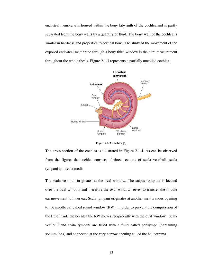
12

endosteal membrane is housed within the bony labyrinth of the cochlea and is partly

separated from the bony walls by a quantity of fluid. The bony wall of the cochlea is

similar in hardness and properties to cortical bone. The study of the movement of the

exposed endosteal membrane through a bony third window is the core measurement

throughout the whole thesis. Figure 2.1-3 represents a partially uncoiled cochlea.

Figure 2.1-3. Cochlea [5]

The cross section of the cochlea is illustrated in Figure 2.1-4. As can be observed

from the figure, the cochlea consists of three sections of scala vestibuli, scala

tympani and scala media.

The scala vestibuli originates at the oval window. The stapes footplate is located

over the oval window and therefore the oval window serves to transfer the middle

ear movement to inner ear. Scala tympani originates at another membranous opening

to the middle ear called round window (RW), in order to prevent the compression of

the fluid inside the cochlea the RW moves reciprocally with the oval window. Scala

vestibuli and scala tympani are filled with a fluid called perilymph (containing

sodium ions) and connected at the very narrow opening called the helicotrema.

13

Between the scala vestibuli and scala tympani there is another channel called the

scala media. The scala media is filled with endolymph (containing potassium ions)

and terminated at helicotrema. Within the scala media are the Basilar membrane and

organ of corti. Organ of Corti is the sensor of pressure vibrations in the cochlea and

is situated on the basilar membrane it is composed of the sensory cells, called hair

cells, the neurons, and several types of support cells.

Figure 2.1-4. Cross section diagram of cochlea [5]

The basilar membrane is a pseudo-resonant structure [12] that, like strings on an

instrument, varies in width and stiffness. The Basilar membrane is widest (0.42–

0.65 mm) with least stiffness at the apex of the cochlea, and narrowest (0.08–

0.16 mm) with highest stiffness at the base [13]. The characteristics of the

membrane at a certain point along its length determine its best frequency, the

frequency at which it is most sensitive. It is most sensitive to High-frequency sounds

at the basal end (near the round and oval windows), while most sensitive to low-

frequency sounds at the apical end.

There are between 16000 and 20000 hair cells along the length of Basilar membrane,

in 4 rows; one row of “inner" hair cells, which are the only ones attached to nerves,

and 3 rows of “outer" hair cells. The inner hair cells transform the mechanical

14

vibration of the basilar membrane into electrical signals that are then transmitted to

the brain via the auditory nerve . However the outer hair cells do not send neural

signals to the brain, but mechanically amplify low-level sound that enters

the cochlea. This amplification may be powered by movement of their hair bundles,

or by an electrically driven motility of their cell bodies [14].

2.2 Hearing Process

The human ear is able to detect sound in the range of 20 Hz to 20 KHz. Much of the

information in speech is in the range up to 3 KHz. The ability to hear high

frequencies above 4 KHz decreases up to 40 dB as the person ages [15]. Hearing is

achieved through a series of procedures in which the ear converts sound waves into

electrical signals and sends the electrical impulses to the brain, where they are

interpreted as sound. Sound travels through the ear canal and pressure of the air

molecules cause the tympanic membrane to vibrate. The ossicular chain is attached

to the tympanic membrane and therefore the movement of the tympanic membrane

causes the ossicular chain to move. The movement of the stapes at the end of the

chain vibrates the oval window on the cochlea, causing the movement of fluid inside

the cochlea. This motion of fluid in turn vibrates the basilar membrane in the scala

media, which causes the hair bundles of the hair cells to move, acoustic sensor cells

that convert mechanical vibration into electrical impulses. After the brain receives

these electrical signals the sound can be heard. Figure 2.2-1 represents the direction

of travel of the sound energy inside the cochlea.

15

Figure 2.2-1. Hearing system [13]

As mentioned above in the normal hearing process the cochlear fluids are stimulated

by acoustic signals travelling through the structures of outer and middle ear and

arriving at the cochlea. This process is called air conduction hearing, as shown in

Figure 2.2-2 [5].

Figure 2.2-2. Air conduction hearing

The cochlear fluid can also be provoked by another process known as bone

conduction hearing. Bone conduction is the process by which as acoustic signal

vibrates the bones of the skull to stimulate the cochlea as presented in Figure 2.2-3

[5].

Figure 2.2-3. Bone conduction hearing

16

2.2.1 Theories of hearing

There are several theories regarding the manner in which sound is perceived by the

human ear. Theories of hearing are as result of the efforts to understand the main

factor causing the frequency discrimination in hearing performed by basilar

membrane movement. According to Lee [16], the following theories are three of the

most common and accepted theories of hearing:

• Place theory: The place theory is based on the assumption that perception of

sound depends on where component frequency produces the maximum

vibrations along the basilar membrane [17]. The place theory is usually

attributed to Hermann von Helmholtz [18, 19]. Later researchers do not agree

that the tuning of the basilar membrane is as sharp as this theory has

assumed, but agree that a particular region of stimulation in the basilar

membrane is responsible for the perception of a particular frequency.

• Frequency (telephone) theory: The frequency theory suggests that all parts

of the basilar membrane are stimulated by every frequency and the frequency

discrimination is based upon the number of times per second that the fibers of

the auditory nerve discharge. However, due to the dissipation of the input

energy in cochlear fluid, the maximum rate of discharge of nerve impulses is

about 1000 Hz. This means that the perception of sound above this frequency

could not be supported on the basis of the telephone theory [20].

• The travelling wave theory: this theory is the most accepted theory of

hearing. The travelling wave theory holds that frequency discrimination

along the basilar membrane is determined when a certain place along the

basilar membrane is set into maximum vibration as a result of the maximum

17

displacement of the travelling wave in cochlea. According to this theory the

energy for creating the travelling wave comes from the stapes, but the wave

starting at one end, runs along the length of the membrane, gradually

increasing in amplitude until it gains maximum displacement. The wave

travels from the base to the apex of the cochlea, and the maximum amplitude

occurs at a point along the basilar membrane that corresponds to the

frequency of the stimulus. Increasing the frequency of the tone moves the

place of maximal vibration toward the base of the cochlea, decreasing the

frequency moves it in the direction of the apex of the cochlea. This is so far

the most accepted theory on the hearing. Support for the travelling wave

theory is contributed by experimentation carried out by George von Bekesy

[21].

2.2.2 Hearing loss

Hearing loss occurs when a person’s ability to detect certain frequencies of sound is

completely or partially impaired. There are three main categories of hearing loss:

• Conductive hearing loss, which limits the mechanical transmission of sound

through the outer or middle ear. It can be treated medically or surgically, and

sometimes a hearing aid can improve the hearing.

• Sensorineural hearing loss, which mainly affects the cochlea or the neural

pathways. In these cases sound is transmitted through the outer and middle

ear normally, but due to damage to the fine nerve endings in the cochlea, the

inner ear might not work properly.

• Mixed hearing loss, which conductive and sensorineural loss occurs at the

same time.

18

In the treatment of hearing disorders not only the cause but also the severity need to

be evaluated. Hearing loss is described as the difference to normal hearing in decibel

(dB). Based on the severity of the hearing loss the conventional hearing aids, ear

implants and cochlea implants are used to treat the problem.

2.3 Conventional Hearing Aids

Conventional hearing aids are the most basic treatment of conductional hearing loss,

which amplify the sound into the outer ear using a speaker. However there are

disadvantages with using this type of hearing aid, which affects the usage of hearing

aids. Currently in UK 1.5 million use a conventional hearing aid of which 62%

report difficulties with their hearing aid [22]. According to Counter [23], the

following five points can be named as the most important disadvantages of

conventional hearing aids:

• Stigma: One of the main reasons which can result in low usage by patient is the

common idea of hearing aid as sign of disability.

• Feedback: The acoustic feedback is caused by the vicinity of the speaker and

microphone and can be recognised as the annoyingly familiar high-pitched

whistle often heard near a hearing-aid user. Improving the seal between the ear

and hearing-aid mould and placing the microphone and the loudspeaker further

apart can break the feedback loop.

• Discomfort: The conventional hearing aid is made of a silicon cast of the

patient’s ear canal and fits into the outer ear. However the cast is not always

precise, therefore many patients complain of discomfort in their ear canal.

Recent rapid prototyping techniques have improved formation of the device.

19

• Difficulty controlling the aid: Due to the small size of the devices, they

become difficult to control especially for elderly people. The new generation of

digital aids has helped to improve this problem, as there is an automatic circuitry

within them [24].

• Occlusion effect: In the standard design of a hearing aid, there is an ear mould,

which blocks the ear canal and can affect it significantly by reduction in the

amount of high frequency entering the ear and change of the resonance

properties of the ear canal.

• Hearing in noise: The majority of hearing aid users have a high frequency loss

and the speaker of the hearing aid is unable to compensate, specifically where

there is much background noise. Digital signal processing in modern aids

compensates for this to some extent, but the amplifier still has to drive a very

small speaker. The response drops off dramatically above 3 kHz and is of no

practical value above 5.5 kHz [23].

2.4 Ear Implantation

The above disadvantages of the conventional hearing aids have directed the

researchers to find a device, which keeps the ear canal free and has less feedback.

Two of the current solutions are middle ear implantation and bone anchored hearing

aid (BAHA), which remove completely the problems with stigma, occlusion and

discomfort.

2.4.1 Middle ear implant

The device is implanted on the middle ear by surgery. Middle ear implantation is

mostly used in the improvement of sensorineural hearing loss. All the current

devices contain four elements of an input transducer like a microphone, an amplifier

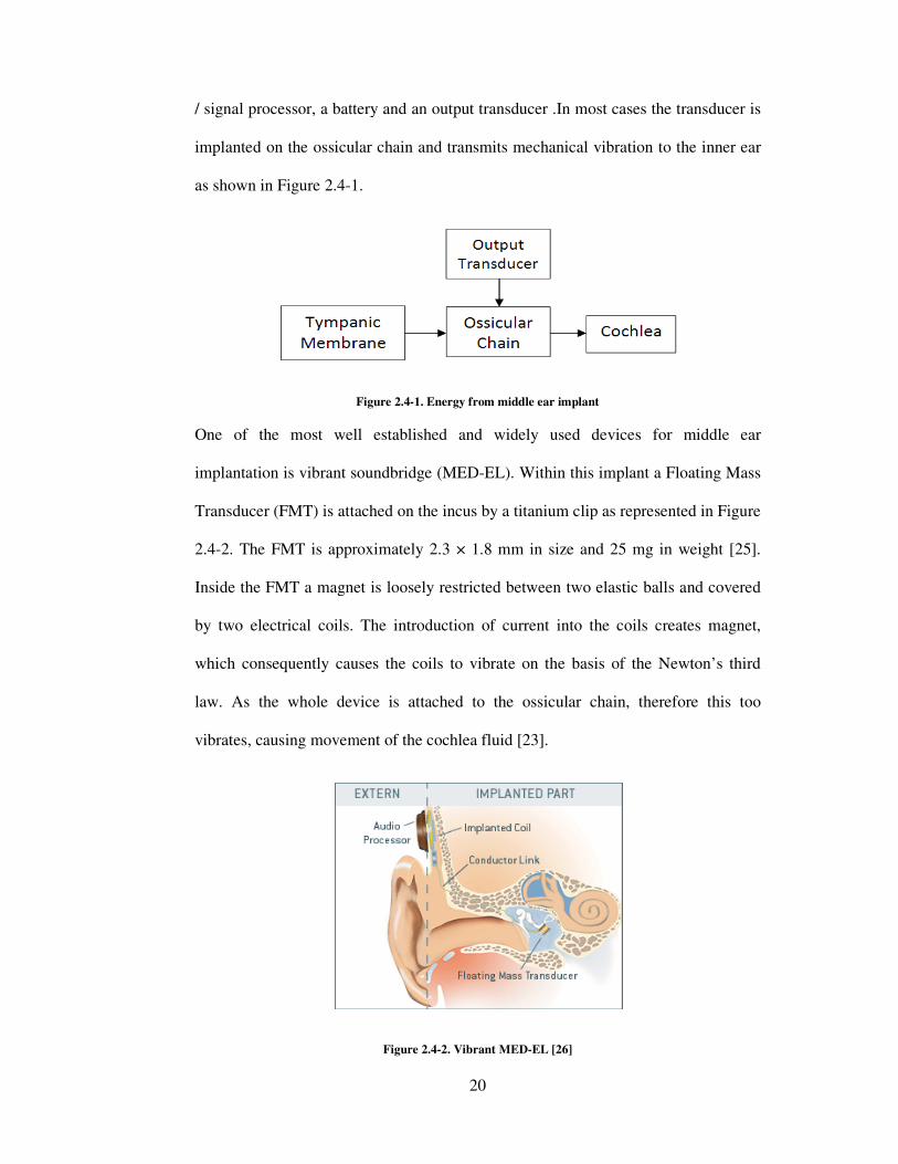
/ signal processor, a battery and an

implanted on the ossicular chain and transmits mechani

as shown in Figure 2.4-1

One of the most well established

implantation is vibrant soundbridge (MED

Transducer (FMT) is attached

2.4-2. The FMT is approximately

Inside the FMT a magnet is loosely restricted between two elastic balls and

by two electrical coils.

which consequently causes

law. As the whole device is attached to the ossicular chain, therefore this too

vibrates, causing movement of the cochlea fluid

20

, a battery and an output transducer .In most cases the transd

implanted on the ossicular chain and transmits mechanical vibration to the inner ear

1.

Figure 2.4-1. Energy from middle ear implant

well established and widely used devices for middle ear

is vibrant soundbridge (MED-EL). Within this implant a Floating Mass

ransducer (FMT) is attached on the incus by a titanium clip as represented in

approximately 2.3 × 1.8 mm in size and 25 mg in weight

Inside the FMT a magnet is loosely restricted between two elastic balls and

by two electrical coils. The introduction of current into the coils create

causes the coils to vibrate on the basis of the Newton’s third


vibrates, causing movement of the cochlea fluid [23].

Figure 2.4-2. Vibrant MED-EL [26]

In most cases the transducer is

cal vibration to the inner ear

for middle ear

this implant a Floating Mass

by a titanium clip as represented in Figure

in weight [25].

Inside the FMT a magnet is loosely restricted between two elastic balls and covered

ils creates magnet,

Newton’s third


21

The small mass of the FMT minimises the effect on the middle ear vibration in terms

of mass loading [27]. However one of the most important disadvantages of these

devices is the dissipation of energy, which results in the short battery life. This

dissipation of energy is due to the travelling of its vibration energy not only toward

cochlea, but also back to the tympanic membrane. Also by implanting a device on

any mechanical part of the hearing chain, there is damping effect on the middle ear.

The other disadvantage with the vibrant soundbridge is the duration and complexity

of its surgical process. If the attachment of FMT is loose on the incus, the device can

be markedly reduced in efficiency.

2.4.2 Bone anchored hearing aid

Another frequently used hearing implant is the Bone Anchored Hearing Aid

(BAHA). It is a surgically implanted hearing aid that works on direct bone

conduction hearing, which propagates sound by conduction through the skull bone

rather than via the outer or middle ear. A 3-4 mm titanium implant, which is placed

in the skull bone (Temporal Bone) behind the ear during a surgical procedure as

illustrated in Figure 2.4-3.

Figure 2.4-3. BAHA implant [28]

22

The sound waves are received by sound processor and the sound processor transmits

sound vibrations physically via the external abutment to the titanium implant. The

vibrating implant causes vibrations within the skull and inner ear that stimulate the

nerve fibres in the functioning cochlea, where hearing takes place.

The BAHA has the advantage over other hearing aids of not occluding the ear canal

or hearing mechanism. It is also less complicated to implant. The amplified sound

delivered by the BAHA is much more efficient than conventional hearing aids in

concept of quality, with improvements in pure tone average hearing levels at 0.5, 1

and 2 kHz varying from 11 dB hearing level to as much as 30 dB hearing level [29].

This is also significant improvement in the discrimination free-field speech [30].

Unfortunately having the implant on the skull raises the stigma problem. Similar to

the Vibrant Soundbridge device the most significant disadvantage of BAHA is the

energy dissipation in the process of transmitting the vibrations through the skull to

the cochlea.

2.5 Cochlea Implantation

The Cochlear Implant is a surgically implanted electronic device inside the cochlea,

which helps people with severe to profound sensorineural hearing loss, or nerve

deafness. Cochlear implant works by directly stimulating any functioning auditory

nerves inside the cochlea with an electric field, unlike hearing aids, which work by

amplifying sound. The configuration of the implant system is shown in Figure 2.5-1.

The cochlear implant has both external and internal parts. The external part is the

microphone and speech processor. The speech processor uses the microphone to pick

up sound from the environment. The speech processor select

prioritize audible speech

to the transmitter. The t

behind the ear, and it sends the signal through the skin to

electromagnetic induction

The internal part is the

surgical procedure. The internal part consists of two main parts. The

receiver/stimulator, which is

signals into electric impulses,

electrode array, which is a group of

stimulator and sends them to different regions of the auditory nerve.

nerve fibres in the cochlea and the signals are recognised by the brain as sound.

23

Figure 2.5-1. Cochlear implantation [31]

has both external and internal parts. The external part is the


up sound from the environment. The speech processor selects and filters

audible speech and sends the electrical sound signals through a thin cable

he transmitter is a coil held in position by a magnet placed

and it sends the signal through the skin to the internal

electromagnetic induction [32].

cochlear electrode implant and is placed inside the ear by a


which is secured in bone beneath the skin and

impulses, then sends them to electrodes. It also consists of

, which is a group of electrodes that collects impulses from the

stimulator and sends them to different regions of the auditory nerve. This stimulates


has both external and internal parts. The external part is the


filters sound to

rough a thin cable

ransmitter is a coil held in position by a magnet placed

internal implant by

e the ear by a


converts the

It also consists of an

that collects impulses from the

This stimulates


24

2.5.1 Cochlear implant surgery

The operation to insert the electrode inside the cochlea is performed while the patient

is under general anaesthesia and it takes from 1.5 to 3 hours to perform the surgical

implantation. Currently implantation is performed manually by an experienced

surgeon. Later on at chapter 7 the disturbances within the cochlea in response to

different procedure during the cochlear implant surgery is investigated. The usual

surgical steps are as follows [33]:

• An incision is made in the crease behind the ear, which makes the scar

inconspicuous once healed.

• A pocket is created under the skin to accommodate the receiver-stimulator

portion of the implant. This part of the implant is flat in form such that it will

not produce a noticeable deformity.

• Using the microscope and a bone drill the bone behind the ear (mastoid bone)

is opened to enable the electrode implant to be inserted. This mastoidectomy

allows us to access the inner ear cochlea without disturbing the ear canal or

eardrum.

• The surgeon then creates a small hole near the RW on the bony wall of the

cochlea, called a cochleostomy. Figure 2.5-2 illustrates the cochleostomy

formation, where an opening is visible through the endosteal membrane.

Figure 2.5-2. Cochleostomy formation [34]

25

• The electrode array is threaded into the scala tympani through the

cochleostomy as far as possible using an instrument provided by the

manufacturer (i.e., claw). Figure 2.5-3 represents the electrode insertion into

the cochlea manually using a claw.

Figure 2.5-3. Electrode insertion [34]

• The receiver/stimulator is secured to the skull, and the incision is closed with

hidden absorbable stitches that do not require removal. The receiver is placed

into a "well" created behind the ear. The "well" helps to maintain position,

and ensures close proximity with the skin to allow electrical information to

be transmitted to the device.

• The incision is closed so that the internal device is beneath the skin.

2.5.2 Hearing preservation cochlear implantation history

Hearing Preservation Cochlear Implant (HPCI) describes the method to preserve

residual hearing (low frequencies) remaining in the cochlea, whilst a cochlear

implant is inserted. Whilst cochlear implantation is extremely successful in

achieving the primary goal of improving speech perception in patients with severe to

profound sensorineural hearing loss, the procedure is not without its limitations.

26

Hearing amongst the persistence of background noise and enjoyment of music

remain a challenge to the cochlear implantation community.

Analysis of the factors determining the success for speech in both quiet and noisy

environment reveals that frequency resolution is critical. Fishman [35] demonstrated

that in a quiet background, top performing CI users only required 3-4 channels of

stimulation for speech perception and once background noise was added, their

requirement greatly increased. Henry [36] compared the frequency resolution of

cochlear implantees patients with sensorineural hearing loss and normal hearing

volunteers. The normal hearing listeners were found to have excellent frequency

resolution of sound, patients with sensorineural hearing loss, and hence damage to

hair cells, had moderate frequency resolution. However the implantee had very poor

frequency resolution. This demonstrated that even when a patient has sensorineural

hearing loss, acoustic reception of sound enables better frequency resolution, and

hence better speech perception, than electrically stimulated hearing. Rubenstein [37]

determined that residual hearing post implantation is one of the few variables that

predict the success of the implantation in terms of speech perception results.

These studies support the concept that if residual hearing is present, then its

preservation will lead to a greater functional result for the implant recipient. Von

Ilberg et al in 1999 was the first to demonstrate that simultaneous ipsilateral hearing

aid and cochlear implant for patients with severe hightone hearing loss and preserved

residual hearing in the low frequencies post implantation, resulted in a significant

increase in speech understanding, compared with a cochlear implant or hearing aid

alone [38]. This presents surgeons with a problem: how to insert an electrode array

into the cochlea, whilst maintaining the implant’s normal function, when during

routine cochlear implantation, a patient’s residual hearing is invariably destroyed.

27

The challenge to preserve residual hearing, whilst inserting a cochlear implant begins

with determining factors that cause hearing loss during implantation.

The cochlea sustains trauma during all the steps of the implantation procedure.

Accessing the middle ear and preparing the implant bed will subject the cochlea to a

combination of noise induced trauma from drill and the cochlea will further sustain a

mechanical/vibrational trauma during this process which may lead to hair cell loss.

Zou demonstrated that a temporary threshold shift, measured by

Electrocochleography, was inducible in guinea pigs by applying vibrations to the

external canal [39]. Performing a bony cochleostomy will again subject the cochlea

to noise and vibrational trauma. Protrusion of a running burr into the scala tympani

will lead to pressure shifts within the cochlea and inadvertent protrusion of the burr

may directly damage the basilar membrane. Suction of perilymph has been shown to

be associated with further sensorineural hearing loss [40]. Insertion of the electrode

may cause trauma either by pressure fluctuations within the scala tympani during

introduction of the electrode array into a closed system, or more likely by damage to

the spiral ligament or penetration of the basilar membrane even if the electrode

originally passed into the scala tympani, or the electrode may be directly passed into

the scala vestibuli [41]. Inserting can lead to new bone formation and fibrosis within

the scala tympani [42].

2.6 Concluding Section

In this chapter a detailed background on the main areas at this work was presented.

This information is vital to help understanding of the work presented in this thesis.

The first part of the chapter describes the anatomy and mechanics of each part of the

ear. The second part describes the process of hearing and the definition of different

28

types of hearing loss. Third and last part of the chapter describes current solutions

for treatment: Namely; conventional hearing aids, middle ear implants, BAHA and

cochlear electrode implantation. The common pros and cons of each solution were

highlighted.

In the next chapter the literature review, will show the merits and advantages of the

present work in contrast to previous work in the field.

29

Chapter 3. Literature Review

This chapter describes relevant literature and place it in context. Topic areas are:

Section 3.1. Introduction: Brief background on the history of the anatomy of the

cochlea.

Section 3.2. Cochlea mathematical modelling: A mathematical model of the

cochlea to help understanding cochlear dynamics.

Section 3.3. Experimental methodology: Description of the third window (TW)

measurement technique.

Section 3.4. Verification of cochlea dynamics: Feasibility of using a TW on the

cochlea as a mean for ear implantation.

Section 3.1. Influence of surgical intervention: Disturbances within the cochlea at

different stages of cochlear implantation.

3.1 Introduction

Until the mid 19th

century, studies on the cochlea were anatomical to identify the

major features of the auditory system, such as, the tympanic membrane, the middle

ear osseous, and the cochlea. In 1963, Du Verney described the coiled basilar

membrane [43]. Improvement of the microscope in mid-1800s was a significant step

toward the discovery of the finer structures of the cochlea. Reissner membrane and

organ of Corti (1851) are now named after the scientists, who identified the nature of

the cochlear structure. Cross section of cochlea and its main structures are illustrated

in Figure 3.1-1.

Since the anatomical exploration of the cochlea, there have been enormous efforts to

understand the dynamics of the cochlea as a whole, and its partitions.

3.2 Cochlea Mathematical M

Over the last four decades many different mathematical models have been proposed

to study cochlear function

access to the cochlear structure

cochlea is to clarify the relationship between the structure and function

Therefore in this work a

displacement of the basilar membrane as a function of distance from the stapes and

endosteal membrane at a

model in contrast to the previous models. First is to simulate the dynamic response

of endosteal membrane at a

secondary set of study the disturbances of the cochlea basilar membrane has been

estimated with the cochlea excited at a

the stapes.

30

Figure 3.1-1. Cross section of the cochlea [44]


understand the dynamics of the cochlea as a whole, and its partitions.

Mathematical Modelling


to study cochlear functions. This is mainly due to the difficulty of experimental

cochlear structure. The main aim of the mathematical model of the

to clarify the relationship between the structure and function.

Therefore in this work a dynamic model of cochlea is outlined to

ment of the basilar membrane as a function of distance from the stapes and

endosteal membrane at a TW. There are two major contributions developed in this


rane at a TW prepared in the bone tissue of the cochlea


estimated with the cochlea excited at a TW on the bony wall as opposed excitation at



. This is mainly due to the difficulty of experimental

tical model of the

estimate the

ment of the basilar membrane as a function of distance from the stapes and

developed in this


the bone tissue of the cochlea. In a


on the bony wall as opposed excitation at

31

The model in this work is a finite-difference approximation of the passive, two-

dimensional cochlea based on the Neely’s approach [45].

In this section the assumptions made in the study and the choice of the numerical

solution is reviewed by previous works and the effects of these assumptions on the

cochlear mechanism are investigated.

3.2.1 Description of cochlear dynamics

Here is a brief descriptive model of the cochlea, aiming to give an overview of the

cochlea mechanism. The basilar membrane separates the cochlear into two channels

which are joined at the apex by the helicotrema. Stapes behaves as a sound stimulus

on the oval window, at the base of the cochlea, causes changes in the pressures

�*+ , , -� and �*� , , -� in both channels. Here - is the time and is the

position along the cochlea, with the oval window at , 0 and the helicotrema

at , ' [46].

Figure 3.2-1. Schematic view of the cochlea [47]

The pressure difference between the channels can be defined as P , �*+ / �*�. The

balance of pressure gradients and inertial forces in the fluid together with the fluid

32

incompressibility and viscosity leads to a relation for the basilar membrane motion

and pressure gradients. The pressure P acts to deform the basilar membrane.

Consequently the basilar membrane displacement can be determined using different

mathematical approaches to estimate pressure differentials.

3.2.2 Passive and active cochlea

Generally two approaches for modelling the cochlear dynamics can be found in the

literature. These approaches are either passive or active [10, 48]. In the passive

model (dead cochlea) the wave travels toward the end of the cochlea and peaks at

frequency dependent locations. At a given excitation frequency the speed of the

travelling wave and its local wavelength decreases as it approaches its peak. In

another word, a travelling wave generated by a sinusoidal excitation travels quickly

in the basal, then slows and reaches a peak at its resonant point where the basilar

membrane impedance is lowest. The location of the peak depends on the input

frequency; thus each point on the basilar membrane has a best frequency.

On the other hand, in the active cochlea, the passive response is amplified by a force-

generating system called the outer hair cells. The outer hair cells are the active

elements of the cochlea and are located on the basilar membrane. In the active

cochlea the wave grows more than in passive case, but with little change in phase

[49].

It is generally accepted that the passive model does not explain the extreme

sensitivity and of the cochlea, even though both active and passive cochleas share a

similar best frequency for a certain input. It is also known that the active processes in

the cochlea plays a role in the amplification of weak signals.

33

Figure 3.2-2 represents the amplification of basilar membrane movement in active

cochlea in contrast to the passive cochlea. As can be observed the active element of

the cochlea also increases the sharpness of tuning.

Figure 3.2-2. Displacement amplification at active cochlea [49]

3.2.3 Geometrical assumptions

Other simplifying assumptions regarding the geometry of the cochlea include;

coiling of the cochlea, presence of the helicotrema, tapering of the cochlea scalae

and cochlea partition motion equations in different dimensions. The consequences of

each of these assumptions are reviewed in this section, based on previous research.

The human cochlea is curled into a spiral that typically exhibits two and a half turns.

A number of authors have considered that the coiling of the cochlea is a secondary

effect on the cochlea mechanism, and so is neglected [50, 51]. They propose that

mammalian cochleae are coiled to pack a longer organ into a small space inside the

skull and that the cochlear coil increases the efficiency of blood and nerve supply

through a central shaft [52].

34

However, Manoussaki [53] modelled the effects of coiling and argued that the

cochlear curvature enhances the radial shearing in the apical end of the basilar

membrane where low-frequency are more present and may enhance sensitivity to

low frequencies by focusing energy towards the outer cochlear wall as waves

propagate towards the apex.

Another geometrical parameter that, until now, has been neglected in most studies is

the effect of the presence of the helicotrema on the cochlear response. Although the

true effect of the helicotrema is not yet fully understood, Marquardt [54] has shown

that the cochlear sensitivity to very low frequency up to 500 Hz [54, 55] is strongly

affected by the helicotrema, an apical connection between the cochlear ducts above

and below the basilar membrane.

Figure 3.2-3 represents the effect of presence of the helicotrema at low frequency of

300 Hz, by Givelberg [55]. It appears that the dip in the amplitude is removed by the

presence of the helicotrema at low frequencies.

Figure 3.2-3. Cochlea response at frequency 300 Hz, (a) with helicotrema, (b) without helicotrema [55]

35

The size of the helicotrema is also debatable, and is believed to affect low

frequencies below 500 Hz [56, 57]. According to this hypothesis, if cochlear fluid

flows through the helicotrema without a loss in pressure, then a pressure difference

will not act across the adjacent cochlear partition and sound will not be detected. It

then follows that smaller areas increases sensitivity to lower frequencies.

Another geometrical factor in cochlea is the tapering of the scalae. In the real

cochlea, the scalae are tapered, with a decreased area at the end of the cochlea, apex

[58, 59]. Figure 3.2-4 illustrates the tapering of the cochlea scalae from the base

toward the apex of the cochlea.

Figure 3.2-4. Tapering of cochlea scalae [60]

There is general agreement on the effect of the tapering of the cochlea scala on the

sensitivity of cochlea response at low frequencies of below 500 Hz [61]. However at

majority of the cochlea models the tapering is neglected and cochlea scalae are

modelled as straight channels. In one study by Steele [51] there was no significant

effect found as a result of the scala tapering.

Based on the points mentioned above, coiling of the cochlea, presence of the

helicotrema and tapering of the cochlea scalae can affect the low frequency response

of the cochlea, and therefore if neglected in the model, the minimum frequency input

of the study should be set higher than 500 Hz.

36

Beyond the above approximations there are attempts to solve cochlea partition

motion equations for different dimensions. Primary one-dimensional models can

provide a good prediction of cochlear response [62], but because of substantial

simplifications they prevent studying fluid effects. Also the absence of direct

structural coupling between the micromechanical elements is a characteristic feature

of classical one-dimensional models of the cochlea. In order to account for fluid

motion more accurately, two-dimensional theories have been put forward, initially

introduced by Siebert’s [63] and Allen’s [64]. In an ample review, Lighthill

considered Allen’s model [64] the best among the two-dimensional ones. Since

Allen, there has been vast number of two-dimensional models [62, 65-68] of cochlea

based on his work. More recently three-dimensional models of cochlea have been

investigated. Much of the three-dimensional works [51, 69-73] require complicate

mathematics and computations, while still rely on simplifying assumptions that deny

much of the physiological reality of the cochlea.

3.2.4 Numerical solutions

So far there are standard numerical solutions for modelling cochlear dynamics such

as the; finite-difference method of Neely [45] and the integral-equation method of

Allen and Sondhi [64]. When analysing the coupled mechanics of the cochlea, due to

the interaction between fluid coupling and motion of cochlear structures, it is convenient

to divide the cochlea longitudinally into a discrete number of sections [74]. Therefore

among all the methods, Neely's explicit finite-difference method is used widely as a

standard numerical method of comparison [67, 68, 75-77].

In finite-difference schemes, the two-dimensional duct is discretized on a $% 0 $&

grid in Cartesian and � directions. The derivatives in the Laplace's equation and in

37

the boundary conditions are replaced by their finite-difference approximations. At

each point, an equation is described for the pressure, in terms of the pressure at the

neighbouring points. Most of the passive cochlea models do not include longitudinal

coupling, and a study by Eze [78] argues that this assumption is appropriate. Figure

3.2-5 represents a 1D lumped segment model of cochlear macromechanics. It is

assumed that in the lumped model that the fluid is uniform across the section of the

cochlea.

Figure 3.2-5. Schematic model of cochlea macromechanics [79]

3.3 Experimental Methodology

Since 1924 there have been numerous efforts to investigate the dynamics of the

cochlea. The majority of measurements have been focused on basilar membrane

motion. The study of the motion of basilar membrane can provide vital information

on what really occurs inside the cochlea in order to transfer vibration energy into

electrical signals. However to reach the basilar membrane an access opening in the

cochlea bone and membrane has to be produced. This will cause cochlear fluid to

drain from the normally closed lumen of the membranous labyrinth of the cochlea

and changes the mechanical properties of the cochlear structures.

38

In this study an experimental rig is proposed to investigate the disturbances within

the cochlea, while keeping the cochlear structures intact. This non-invasive

measurement method has been possible as a result of using the robotic micro-drill

[80, 81] to create an aperture through the bony cochlear surface, onto the underlying

endosteal membrane. Further details on the characteristics of the micro-drilling

technique are given in chapter 5. As mentioned previously there are already two

natural windows onto the membrane. There are the round and oval windows

respectively. The aperture created for the experiments in the bony wall of the

cochlea, will be referred to as “Third Window (TW)”. Figure 3.3-1 illustrates such

third window created on the cochlear surface. As can be observed the exposed

endosteal membrane remains intact.

Figure 3.3-1. Bony cochlea third window

Using this rig, it is possible for the first time to observe real transients corresponding

with actuation of the hearing chain and disturbances induced by the insertion of

hearing implants without invading the cochlear space. The significance of the

proposed measurement method of this work is that the dynamic behaviour of the

cochlear endosteal membrane can be investigated without affecting the natural

structure of the cochlea.

39

In this technique disturbances within the cochlea are investigated at a third

membrane window produced in the bony wall of the cochlea by the robotic micro-

drill. Motion of the membrane reflects pressure disturbances in cochlear fluid. The

robotic micro-drill developed within research group, guarantees the integrity of the

underlying endosteal membrane that is used as a pressure transducer diaphragm.

Micro-Scanning Laser Vibrometer (MSV) is employed through a microscope that

enables measurements on displacement velocity.

3.3.1 Previous cochlear measurement techniques

Within this section different measurement techniques used by researchers are

reviewed, and the pros and cons of each method are briefly mentioned.

George von Békésy was the first person to make direct measurement of the basilar

membrane from 1924 for which he received a Nobel Prize in 1961 [21]. His method

incorporated new micro dissection techniques and stroboscopic illumination to

investigate the propagation of travelling waves in cadaver cochlea subjected to a

pure tone. The limited sensitivity of this technique essentially restricts observations

to vibration amplitudes greater than 1 1m and required the application of intense

stimuli. Von Békésy concluded that vibrations were not sharply tuned; meaning that

a wide range of frequencies could evoke a notable response from a specific place on

the basilar membrane. Since 1924 numbers of methods have been developed to

achieve more accurate measurements of cochlear dynamics, and mainly the basilar

membrane. Below are the main measurement techniques and their relative pros and

cons [82].

Mössbauer Technique: In 1967, the sensitive Mössbauer technique was used to

measure basilar membrane motion in living animals by Johnstone and Boyle in 1967

40

[83], and by Rhode in 1970 [84-86]. The first in vivo recordings of basilar

membrane vibrations [83] as well as the discovery [84] and early descriptions of

compressive nonlinearities of cochlea [87-91] were carried out using this technique

[82].

At the Mössbauer technique a small source of gamma photons is placed on the

location of the measurement (e.g. basilar membrane), and a resonant absorber, tuned

to the energy of photons emitted by the source at or near rest, is interposed between

the source and a detector. With such configuration, the rate of detected photons is a

function of the velocity of the source [82, 84, 89]. Rhode's data appears more sharply

tuned than the cadaver data of von Békésy. Rhode also concluded that the

experimental condition of the animal subject can effect sharp tuning.

The main disadvantages of the Mössbauer technique is nonlinearity in the function,

therefore undistorted velocity measurements are only possible over a narrow range

of response magnitudes. There are also the difficulties over low signal-to-noise ratio,

the load on the cochlear partitions, and possible radioactive damage [92].

Capacitive Probe: This technique, was first employed by von Békésy [21] and

measures the capacitance that between a fixed electrode and the basilar membrane,

when distanced by a nonconducting gap like air. Basilar membrane vibrations cause

changes in capacitance, which in turn modulates a radio-frequency carrier signal [21,

93]. Even though this method is very sensitive and linear, it requires the removal of

most of the cochlear fluid at the measurement site so that the basilar membrane

remains covered only by a thin film of fluid. This measurement method is not

possible without causing a lot of damage to the cochlear structures [82].

41

Fibre Optics: The motion of the cochlea partitions have also been measured using a

fibre-optic displacement sensors [94, 95], which is placed proximity to the basilar

membrane [96]. The probe consists of one or more central fibres that deliver light to

the target and surrounding fibres that receive reflected light. It is difficult to position

the sensor close to the basilar membrane with no damage to the basilar membrane.

There will also be a load on the membrane by the reflector [82].

Laser Doppler Vibrometer: More recently a widely used method for cochlear

mechanical measurement is laser interferometry [97-101]. Laser interferometry and

its variations are probably the only techniques currently available in the hearing

research community to non-directly measure the motion between the elements of the

cochlea partitions. The most important advantages of this technique are the high

sensitivity and the linearity of the laser interferometer, which gives this technique a

wide dynamic range and high signal to noise ratio. These factors are vital points on

the measurements of the cochlea. In this technique the target velocity may be

extracted by frequency demodulation [102, 103], much as implemented in

commercially available Doppler-shift Laser Vibrometer [101, 104]. Laser

vibrometers are usually used via a microscope to compensate to target the laser beam

on the micro structures of the cochlea [101, 104-106]. As the reflection coefficient of

cochlear partitions are extremely low, approximately 0.0039-0.033% [107] therefore

the laser interferometry technique requires the placement of reflective objects (e.g.

gold crystals, micro beads or metallic paint) to make up for the transparency of the

cochlear partition. This raises the argument of whether these reflective objects follow

the movement of the cochlear partition. A study by cooper has suggested no

significant difference between the motion of micro beads located on the basilar

membrane and adjacent sites of the basilar membrane [105, 108].

42

In general, regardless of the difference measurement techniques, all the results share

a similar conclusion on the motion of the basilar membrane. Low frequency sounds

invoke higher response at the apex of the cochlea whereas high frequency invokes

greater response near the base of the cochlea. The tonotopic arrangement of

frequency recognition within the cochlea is achieved through changes in basilar

membrane mass and stiffness. The stiffness of the membrane is maximum and

lightest at the base with a gradual progressive change to least stiff and heaviest at the

apex. Figure 3.3-2 represents the tonotopic arrangement along the cochlea path

[109].

Figure 3.3-2. Approximate frequency map (in kHz) on the basilar membrane [18]

3.3.2 Round window (RW) measurements

There have also been measurements at the RW opening. The study on the RW

vibration is the only means of measurement on the sealed cochlea within studies

previous to this work. In 1982 Su [110] made the first precise histological

measurements of the cochlear aqueduct, RW membrane, RW niche. As one would

assume in a simple mass spring system, at low frequencies, fluid volumetric

43

displacement at the oval window equals that at the RW but with opposite phase. This

hypothesis is supported by the experimental results of Kringlebot and Stenfelt [111,

112]. It is also suggested that the vibration of the stapes footplate and the

corresponding fluid displacement is a measure of the input energy to the cochlea

[113]. In principle this can be used to estimate the level of stimulation of the cochlea

[114]. Currently the most optimised approach to estimate the volume displacement

of the RW is by measuring the velocity of a single position membrane using a Laser

Doppler Vibrometer [112].

There are also studies on both the displacement or sound pressure level (SPL) at the

RW in response to the different surgical method used at cochlea implantation process

[115, 116]. These studies are all performed to have better understanding of the

different surgical approached on the mechanical function of the inner ear.

However the RW merely provides a single point of measurements and it is not

possible to contrast the disturbances along the length of cochlea.

3.4 Verification of Cochlear Dynamics

The feasibility of placing middle ear implantation to a location on the hearing organ

(cochlea) has been investigated in respect to reduce the energy dissipation and longer

battery life of the implant.

The middle ear implant is a recent addition to the range of hearing aid device for

treatment of deafness. In the current practice, the implant is a micro actuator that is

designed to be clipped to the incus of the ossicular chain within the middle ear such

as Floating Mass Transducer (FMT) of vibrant Soundbridge MED-EL as shown in

Figure 3.4-1.

44

Figure 3.4-1. FMT placement on incus [117]

Synthesised mechanical excitation at this point in the hearing mechanism is

transmitted through the remainder of the serial chain; the incus, the stapes, fluids of

the inner ear to the receptors of the cochlea hearing organ. In addition, vibratory

energy is transmitted back up to the tympanic membrane and through other adjacent

structures and this is a loss to the system.

The mass of the FMT is 25 mg, and damping of stapes movement becomes

measurable in vitro at 500 Hz. This damping raises with increasing frequency,

approaching a 10–20 dB loss at 5 kHz. However the position of the FMT on the

incus has a direct effect on the damping [23, 118].

Another popular ear implant is the Bone Anchored Hearing Aid (BAHA), where the

actuator is implanted on the tympanic bone of the skull. Similar to the vibrant

Soundbridge device the most significant disadvantage of BAHA is the energy

dissipation needed to transmit the vibrations through the skull to the cochlea. Figure

3.4-2 illustrates the transition of energy from BAHA to the cochlea bone through the

skull.

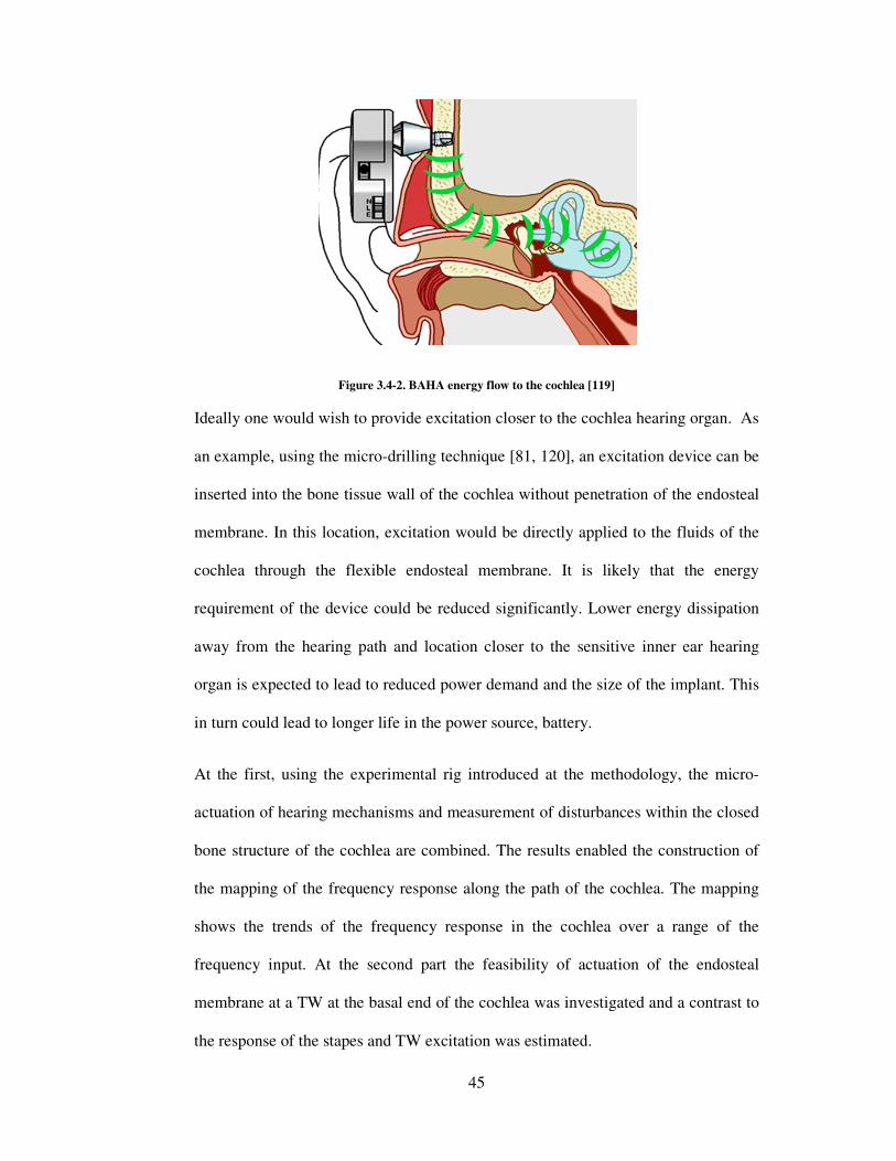
45

Figure 3.4-2. BAHA energy flow to the cochlea [119]

Ideally one would wish to provide excitation closer to the cochlea hearing organ. As

an example, using the micro-drilling technique [81, 120], an excitation device can be

inserted into the bone tissue wall of the cochlea without penetration of the endosteal

membrane. In this location, excitation would be directly applied to the fluids of the

cochlea through the flexible endosteal membrane. It is likely that the energy

requirement of the device could be reduced significantly. Lower energy dissipation

away from the hearing path and location closer to the sensitive inner ear hearing

organ is expected to lead to reduced power demand and the size of the implant. This

in turn could lead to longer life in the power source, battery.

At the first, using the experimental rig introduced at the methodology, the micro-

actuation of hearing mechanisms and measurement of disturbances within the closed

bone structure of the cochlea are combined. The results enabled the construction of

the mapping of the frequency response along the path of the cochlea. The mapping

shows the trends of the frequency response in the cochlea over a range of the

frequency input. At the second part the feasibility of actuation of the endosteal

membrane at a TW at the basal end of the cochlea was investigated and a contrast to

the response of the stapes and TW excitation was estimated.

46

At the previous researches there have been efforts to stimulate the cochlea in a

reverse manner, i.e., by round-window stimulation. Next section will review the

previous works on RW stimulation.

3.4.1 Round window implantation

Coupling of the FMT to the incus in patients with sensorineural hearing loss can

improve the hearing in many cases of middle ear pathologies, but has a significant

energy dissipation and failure rate [121].

Recently, there have been attempts to place the FMT at the RW as an alternative

approach of introducing sound to the cochlea. Figure 3.4-3 illustrates the FMT

placement on the incus bone and the RW.

Figure 3.4-3. Placement of FMT on the incus and round RW [122]

Recently, Colletti implanted the FMT, into 7 patients to stimulate the RW [123],

which improved their speech intelligibility [121].

Kiefer [124] investigated the coupling of the FMT o the RW in a patient with a

malformed ossicular chain. The outcome suggested that the improved thresholds

were 15 to 30 dB better in the frequency range of 750 to 6,000 Hz.

47

The recent publications reporting the implantation of the FMT on round window

vary significantly in outcome, likely due to the variety of pathologic conditions and

inconsistency in the FMT-RW coupling. However, none of these reports mention

likelihood that the presence of the FMT altered the ability of the RW to move,

causing the balance of impedance of the two scalae to change [121].

Another important factor in FMT-RW implantation is that the motion of the FMT

implanted on the RW can be limited by the bony overhang surrounding the RW.

Therefore in most cases this bony overhang is partially removed to allow the FMT’s

flat circular surface to abut the RW [121, 123]. This could be a risk to damage the

RW and cochlea structure during the drilling process.

A recent study by Shimuzu [125] also reviewed that dispersion of the energy

transmitted by the FMT, when attached to the RW membrane is greater than when

the bony stapes footplate is stimulated. Therefore it can be concluded that even

though RW attachment is an alternative to the incus placement more study is

required to identify optimal location of implantation at a TW produced in the bony

wall of the cochlea.

3.5 The Influence of Surgical Intervention

Disturbances within the cochlea caused by different steps of cochlea implantation are

explored using the TW measurement technique, with methods of minimizing trauma

suggested in respect to hearing preservation.

Standard cochlear implantation is an extremely successful intervention for patients

with bilateral, severe to profound, sensorineural hearing loss. Figure 3.5-1 illustrates

the surgical stages in current cochlear implantation. In A, a skin flap incision is made

48

behind the ear. In B, after an intact canal wall mastoidectomy is performed, the facial

recess is opened. A cochleostomy is then created by drilling anterior from the RW

into the basal turn of the cochlea. In C, an electrode array is placed in the cochlea

[126]. Currently all the process is done manually with little knowledge of the relation

of the method and the trauma it might cause within the cochlea.

Figure 3.5-1. Drawings illustrate surgical technique [126]

Hearing Preservation Cochlear Implantation (HPCI) is the focus of much interest in

the cochlear implantation community. Whilst conventional hearing aids greatly

benefit those with mild to moderate hearing losses, HPCI is intended to aid those

patients who cross the borders between these 2 groups, i.e. patients with mild to

moderate hearing losses in the low frequencies and severe to profound losses in the

high frequencies. HPCI requires insertion of an implant electrode array whilst,

ideally, maintaining the patients current hearing levels. This is technically difficult as

hearing loss can be caused at many stages throughout the implantation process, and

is most likely due to an additive effect of these insults [42].

Until recently, complete loss of residual hearing was a typical outcome of cochlear

implantation procedure. However, recent efforts at hearing conservation have

demonstrated that it is possible to preserve the residual hearing in the majority of

cases [127]. HPCI is achievable with many authors having published data with

49

varying degrees of hearing preservation achieved during the implant procedure. The

success rates vary between preservation in 100% with 6mm and 10 mm electrodes in

6 patients [128], to preservation in 50% with 17 mm insertion [129]. Even in the

patients whose hearing is preserved, there is a wide range of hearing levels varying

from 0.7 dB [130] hearing loss to 40 dB [131] hearing loss.

The ideal situation would be to preserve the entire patient’s existing hearing, at the

cochlea implantation process. To achieve this aim, trauma to the cochlea has to be

controlled, and minimized, at all stages of the implantation process such as;

cochleostomy formation and electrode insertion.

3.5.1 Cochleostomy drilling

The main aim of this study is to give a clear contrast between the current manual

method used to create a cochleostomy and the cochleostomy performed by the

robotic micro-drill. A comparison was also made on the influences of the drilling

force and speed on the disturbances within the cochlea. This is the first study as such

to investigate the cochlea dynamics during the cochleostomy formation. This

knowledge will allow implementation of strategies to minimize these disturbances,

leading to greater preservation of residual hearing.

Drilling the cochleostomy is considered to be one of the critical steps at cochlear

implantation procedure. In the current practice the cochleostomy is made manually

using a 1.0 or 1.5 mm diamond burr, inferior and anterior to the RW membrane. The

thin endosteal membrane is on the inner surface of the bony wall of the cochlea.

Under the endosteal membrane are the cochlear fluids which move in the presence of

sound and are vital for of hearing. The endosteal membrane needs to be perforated to

insert the electrode array. At the current procedure this step of the operation is

50

performed by hand, with the membrane being perforated by the drill in over 60% of

cases [132]. Figure 3.5-2 illustrates the cochleostomy drilling on the bony wall of the

cochlea.

Figure 3.5-2. Drilling a cochleostomy [127]

Drilling of a cortical mastoidectomy, implant well, posterior tympanotomy and bony

cochleostomy will all subject the cochlea to noise induced trauma from drill noise

[116]. Further, the cochlea will sustain a mechanical/ vibrational trauma during this

process which may lead to further hair cell loss [39].

The exposure of the inner ear during cochleostomy formation causes SPLs up to 110

dB that could destroy any residual hearing remaining in the cochlea. However the

acoustic trauma may be dramatically high when a running burr touches the intact

endosteal membrane and once the membrane is exposed, sound pressure peaks up to

more than 130 dB [116]. This study also suggests that larger burrs and drilling speed

cause higher SPLs.

Lenhardt recommends the ideal way to minimize trauma during cochleostomy

formation is to perform a bony cochleostomy preserving the underlying endosteal

membrane, which is subsequently opened with a pick/knife rather than a running

burr. This method avoids introducing a running burr into the scala tympani [133].

51

The force controlled robotic micro-drill [134], controls force during the drilling

process by manipulating the linear movement (out to in) of the drill, this dictates the

force of the burr on the bone and therefore the force can be kept constant, within

strict limits. By sensing the changes in force and torque transients during the drilling

process, the robotic micro-drill can reliably stop on the interface of bone and soft

tissue, preserving the endosteal membrane. This process also minimizes any jolting

of the burr caused by the initial impact of a running burr against the bone.

3.5.2 Electrode insertion

The principal aim of this investigation is to compare between the manual and robotic

insertions of the electrode on the disturbances within the cochlea. The robotic

insertion is performed at different speeds to investigate the effect of controlled

insertion speed on the disturbances within the cochlea.

At the insertion process, the electrode array is threaded into the scala tympani by

diameter of approximately 0.6 mm through the cochleostomy near the RW as far as

possible, manually using an instrument provided by the manufacturer (i.e., claw).

Figure 3.5-3 represents an electrode array fully inserted inside the cochlea.

Figure 3.5-3. Electrode curls into the cochlea [135]

52

The electrode is gently pushed into the cochlea by hand and precise technique

specific to each manufacturer’s device is followed. Cochlear electrode insertion is a

challenging manual procedure. The outcome of the cochlear implant depends on

preserving delicate cochlear structures while accurately inserting the electrode array

inside the cochlea up to full 2 turns.

Two of the main goals to achieve at electrode insertion procedures are to insert

electrode arrays into the cochlea without any trauma or damage to the intracochlear

structure and to increase electrode insertion depth of up to two turns.

Since the first use of the cochlea implant there have been investigations on different

aspects of the electrode insertion. For a long time the research has focused on the

design of electrodes and some of the considerations associated with electrode design

are: electrode placement, number of electrodes and spacing of contacts, orientation

of electrodes with respect to the excitable tissue, and electrode configuration. At

present electrodes differ in overall length, diameter, contact design and distribution

as well as stiffness [136].

Another area of interest is the cochleostomy site, in order to place the electrode

safely within the cochlea and to minimise damage to the structure and basilar

membrane [137].

Membrane rupture forces are below thresholds of human tactile perception. Recently

there are efforts to measure the force induced to the scala wall by the tip of the

electrode and also create a device to insert the electrode inside the cochlea with

respect to the position of the electrode tip by measuring the force applied to the tip

[138, 139]. This method usually works by placing force sensors on the tip and along

the electrode and evaluating the curling behaviour of it. However none of these

53

methods provide any information on the shape of the electrode, and its location in

regards to the inner cochlea structures (e.g. basilar membrane) while insertion.

Trauma to the spiral ligament or penetration of the basilar membrane can occur after

the electrode has passed into the scala tympani, or the electrode may be directly

passed into the scala vestibuli [41].

There has also been research on the influence of a cochlear implant electrode on the

mechanical function of the inner ear. In a study by Huber [140], the intraoperative

measurements of the stapes with the RW before and after cochlear implant were

compared and no significant changes in amplitude and phase were seen at the stapes

and RW after cochlear implantation. In another study by Donnelly [141] the impact

of cochlear implant electrode insertion on middle-ear low frequency function was

investigated. Although the results of this study were not consistent it concluded that

the insertion of a cochlear electrode implant produces a change in stapes

displacement at low frequencies, which may have an effect on residual low

frequency hearing thresholds.


In this chapter a literature review of relevant previous work to the presented works of

this thesis was discussed. At the start of each section the aim of the study was

demonstrated and the specific contributions in contrast to other works are

highlighted.

• Modelling of the cochlea: the current models have been discussed including

the various geometrical assumptions and numerical solutions selected by

researchers. It is understood that the assumptions and numerical solution

54

chosen for the mathematical model in this study are sound for the specified

frequency range.

• Experimental methodology: different measurement techniques employed

by the previous studies were considered and pros and cons of each study

were noted. At this study the TW measurement technique is designed, which

unlike the previous methods does not invade the endosteal labyrinth and that

provides the possibility to evaluate pressure disturbances at different sites of

the cochlear membrane.

• Verification of cochlea dynamics: The potential to locate an implant

actuator precisely as required suggests that one should be seeking the ideal

location. Lower energy dissipation away from the hearing path and location

closer to the sensitive inner ear hearing organ is expected to lead to reduced

power demand and the size of the implant. In this study a mapping of cochlea

dynamics is provided using the TW measurement, which can be applied to

determine an optimal implant location in respect to the frequency range of

hearing loss.

• Influence of surgical intervention: Currently the insertion of the electrode

array in cochlear electrode implantation is accomplished manually by the

surgeon, and results in insertion at an unknown speed with possible effect on

the cochlear membrane. In this study the affect of using different surgical

approaches in cochlear implantation on disturbances induced within the

cochlea is contrasted with the use of robotic tools in respect to hearing

preservation.

55

Chapter 4. Mathematical Model of the Cochlea

To obtain a full understanding of the mechanism and behaviour of the fluid, structure

and pressure transients within the cochlea one cannot depend on experimental

measurements alone. A mathematical simulation model will enable the significance

of individual parameters to be assessed. To meet this aim a model has been

developed in this work that takes the following into account; the motion of the oval

and round window (RW), motion of the basilar membrane (BM) and motion of the

endosteal membrane at a third window (TW) through the cochlea bony wall, based

upon pressure and inertia.

The cochlea is the principal part of the inner ear, where mechanical vibrations

(forced by sound waves in the air) are transformed into electrical neural signals. The

cochlea has a spiral shape resembling the shell of a snail. The uncoiled cochlea is

shown in Figure 4-1, representing the terminology, abbreviation used in this chapter.

Figure 4-1. A schematic view of the uncoiled cochlea, showing the terminology, abbreviations. Adopted

from [47]

Unravelled, the cochlea's hollow tube is approximately 35 mm long and 2 mm in

diameter. The tube of the cochlea is divided into three sections: the scala vestibuli,

56

the scala media (or cochlear duct) and the scala tympani. The three scalae wrap

around inside the cochlea. The scala vestibuli forms the upper chamber and at the

base of this chamber is the oval window that is excited by the stapes. The lowermost

of the three chambers is the scala tympani. It too has a basal aperture, the RW. The

scala media separates the other two chambers along most of their length. The start of

the cochlea, where the oval and RW are located is known as the basal end, while the

other end is known as the apical end (or apex). The scala vestibuli and the scala

tympani communicate with one another via the helicotrema, an opening in the

cochlear duct at the apex.

Both scala vestibuli and scala tympani are filled with the same fluid, known as

perilymph, while the scala media is filled with endolymph. Figure 4-2 shows the

intact endosteal membrane, which at the normal form is cover by cochlear bone.

Figure 4-2. Intact endosteal membrane

Between the scala tympani and the scala media is the basilar membrane. The basilar

membrane is narrow, thick and stiff at the basal end and wide, thin and flexible at the

apical end. The cochlea structure is packed together by a 0.1-0.2 mm thick [11]

membrane called Endosteal membrane. The endosteal membrane is housed within

57

the bony labyrinth of the cochlea and is partly separated from the bony walls by a

quantity of fluid.

In Chapter 2, the anatomy and function of the cochlea, and the previous works on the

measurements of cochlear dynamics are described in more detail. Several numerical

solutions for the mathematical model of the cochlea have been proposed. Neely’s

finite-difference method [45, 142], provides a fundamental foundation to the study of

the cochlea and is widely accepted as a sound research base [67, 143] . In Neely’s

approach, the two-dimensional duct is divided into a $% 0$& grid of points. The

continuous derivatives appearing in Laplace's equation and in the boundary

conditions are replaced by their finite-difference approximations. At each point, an

equation is written for the pressure, in terms of the pressure at the neighbouring

points [75].

In this chapter a finite-difference approximation of the passive cochlea model, with

consideration of the principal physical features of the human cochlea is outlined

based on the Neely’s approach. The model is used to estimate the displacement of

the basilar membrane as a function of distance from the stapes and endosteal

membrane at a TW. The primary aim of this mathematical model is to help

understand the mechanism of the cochlear and the relationship between the structure

and the function of the cochlea In contrast previous works, the model is extended to

enable relevance to the aim of the work. The model is used to simulate the dynamic

response of endosteal membrane at a TW prepared in the bone tissue of the cochlea.

Using the model the effect of different locations of the window on the disturbances

of the basilar membrane has been estimated. In a secondary set of study the

58

disturbances of the cochlea basilar membrane has been estimated with the cochlea

excited at a TW on the bony wall as opposed excitation at the stapes.

In the model appropriate assumptions on the stiffness of boundary conditions have

been made in order to simplify the dynamics. Similar characteristic trends are found

on comparing predictions of the model to measurement in practice. The geometrical

assumption made in the study, the choice of the numerical solution and the effect of

these assumptions on the cochlea mechanism are reviewed in details at chapter 3.1.

4.1 Formation of the Model

The model described in this study is a linear, Time-invariant, lumped-element

representation of the passive cochlea based on [50, 90, 91] human parameters.

Due to the interaction between fluid coupling and motion of the cochlea structures, the

cochlea is assumed longitudinally decoupled. By this, one implies that membranes

can be divided into number of thin segments and allows the equations that describe

the motion of a single section of the membrane to be independent of the equations

that describe the motion of other sections along its length [67, 68, 74-77, 144].

Even though the single sections of the cochlea are assumed to be structurally

independent, but the motion of the nearby elements are coupled to one another via

cochlea fluid. A number of assumptions are inherent for the cochlea fluid to this

representation of cochlea micromechanics. First the cochlea fluid is defined as

inviscid (lossless), which implies that sound energy is not dissipated in the bulk of

the fluid, and is transferred into the motion of the basilar membrane [145]. Second,

the fluid is incompressible. The incompressibility of the fluid disallows the existence

59

of compression waves, waves within the cochlear fluid which travel at a high

velocity [67].

Other simplifying assumptions regard the geometry of the cochlea. The cochlea is

coiled in most mammals, providing a more compact and rigid structure. A number of

authors have argued that the coiling of the cochlea is a secondary effect on the

cochlea mechanism, and so is neglected [50, 51]. They proposed that mammalian

cochleae are coiled to pack a longer organ into a small space inside the skull and

that the cochlear coil increases the efficiency of blood and nerve supply through a

central shaft [52]. However, based on Manoussaki’s research [53] modelled may

enhance sensitivity to low frequencies of below 400 Hz by focusing energy towards

the outer cochlear wall as waves propagate towards the apex.

At this study a rectangular model of the cochlea is assumed based on a Cartesian

coordinate system. Figure 4.1-1 represents the physical two-dimensional model of

the cochlea. The model demonstrates both chambers of the cochlea.

Figure 4.1-1. The physical two-dimensional model of the cochlea. Adopted from [143]

In this work the cochlea is treated as a two-dimensional system based on Allen’s

model [64]. This indicates that all the pressures across the section are considered

60

uniform. The model is in two symmetrical parts. The parts are separated by an elastic

partition referred to represent the basilar membrane and will be deformed by a

pressure difference across it. The basilar membrane will have stiffness; mass

properties and damping that vary along its length along cochlea. The top and bottom

part of the model are the endosteal membranes covered by the cochlea bone. The

cochlea bone is assumed to be rigid and therefore there is no fluid flow in a direction

normal to the hard wall.

The other main factor, which needs to be discussed, is the tapering of its scalae. In

the real cochlea, the scalae are tapered, with a decreased area at the end of the

cochlea, apex [58, 59]. There is a general agreement on the effect of the tapering of

the cochlea scala on the low frequencies of below 500 Hz [61] at this model the

scalae cross sectional area is assumed to be constant, which is fine as the frequencies

below 500 Hz are not included in the study.

In Figure 4.1-1 the helicotrema is on the right side of the model. The helicotrema

connects the cochlea channels at the apex of the cochlea, and have an area of

approximately 0.15 ##23125. It has a significant impact on low-frequency auditory

sensitivity due to its influence on cochlear input impedance. Most of the current

cochlear models that have used the straight cochlear map have apical reflections and

therefore standing waves for frequencies below 500 Hz. Apical reflections are

directly related to the low-frequency limit of the cochlear map. Consequently

cochlear sensitivity to very low frequency up to 500 Hz [54, 55] is strongly affected

by the helicotrema.

For frequencies above 500 Hz this boundary condition is of little consequence,

because the pressure has dropped nearly to zero due to losses in the basilar

61

membrane displacement, therefore the solutions to the model are not sensitive to the

choice of apical boundary condition for frequencies above 500 Hz [146]. This work

follows Allen’s assumption that the pressure is zero at the helicotrema for the

frequencies above 500 Hz [64].

Stapes movement is the displacement input to the cochlea, which is a replica of the

sound pressure disturbances in the air outside the ear canal. Very slow vibrations of

the stapes result in a movement of fluid between the scala vestibuli and the scala

tympani through the opening at the helicotrema. Higher frequency vibrations are

transmitted through the yielding cochlear partition as a result of the incompressibility

of the fluid.

The average fluid volume displacements at the RW and oval window are measured

to be within 3 dB of each other for frequencies below 1 kHz; above 1 kHz, the fluid

volumes displaced at the two windows were approximately equal [111, 114]. In this

model it is assumed that the volume displacement at the RW is equal and opposite

direction to that initiated by the stapes footplate.

The model is symmetrical in the two chambers, therefore we can consider only one

chamber, as shown in Figure 4.1-2; however, we must account for the displaced fluid

mass. The length dimension of the model runs from x , 0 to x , L, and the height

dimension runs from y , 0 to y , h, as shown.

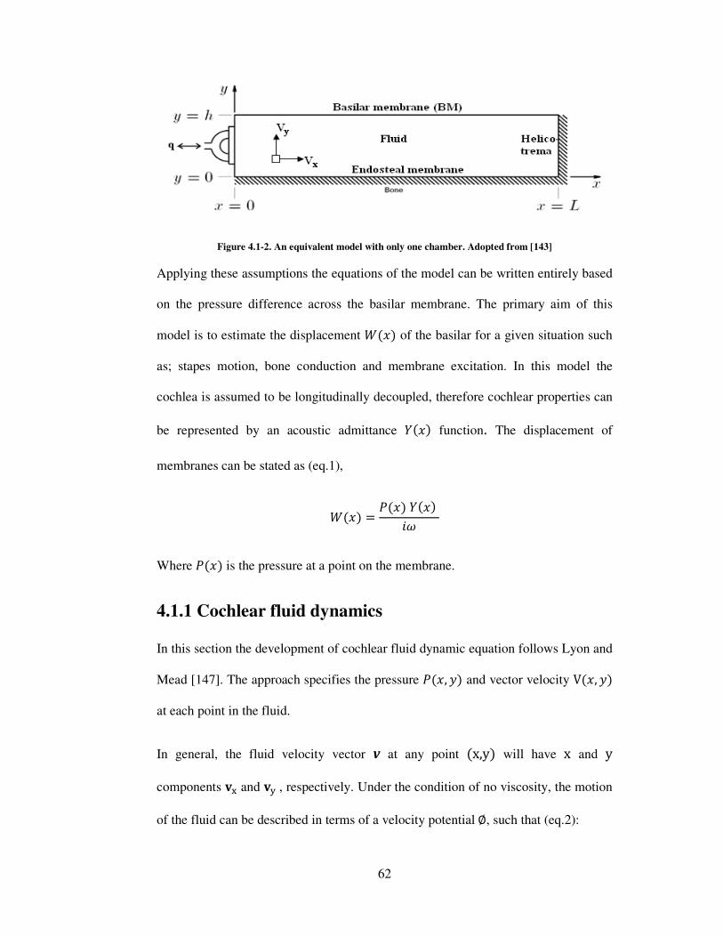
62

Figure 4.1-2. An equivalent model with only one chamber. Adopted from [143]

Applying these assumptions the equations of the model can be written entirely based

on the pressure difference across the basilar membrane. The primary aim of this

model is to estimate the displacement �� of the basilar for a given situation such

as; stapes motion, bone conduction and membrane excitation. In this model the

cochlea is assumed to be longitudinally decoupled, therefore cochlear properties can

be represented by an acoustic admittance �� function. The displacement of

membranes can be stated as (eq.1),

�� , �� :�

Where �� is the pressure at a point on the membrane.

4.1.1 Cochlear fluid dynamics

In this section the development of cochlear fluid dynamic equation follows Lyon and

Mead [147]. The approach specifies the pressure �, �� and vector velocity V, �� at each point in the fluid.

In general, the fluid velocity vector v at any point x,y� will have x and y

components ;< and ;= , respectively. Under the condition of no viscosity, the motion

of the fluid can be described in terms of a velocity potential �, such that (eq.2):

63

v< , /d�dx And (eq.3)

v= , /d�dy

The fluid is assumed to be incompressible and with a volume density (�). Also from

volumetric continuity, @ can be represented as the gradient of a scalar function � as

shown in (eq.4):

@ , /A"�B � , /C�

As a result the flow into and out of any region must balance the velocity field must

neither converge nor diverge, so (eq.5):

div @ , E.@ , BGB H BG�B� , 0

And in terms of the velocity potential it can be written as (eq.6),

B:G A"�B � , EI� , BI�BI H BI�B�I , 0 The well known Newton’s second law of motion can be written to relate the inertial

force to acceleration via mass, J , #�. By considering a small element of the fluid

and the force acting on it from stapes motion it is shown that the pressure K in the

incompressible fluid is related to the derivative of fluid velocity by the relations

(eq.7)

/BKB , � B@LB-

64

And (eq.8)

/BKB� , �B@MB-

Where K is the pressure in the cochlear fluid. By substituting eq.2 and eq.3 into eq.7

and eq.8, the relationship between the pressure and the velocity potential at any point

of the fluid can be written as (eq.9):

K , � B�B-

Where K is the deviation from the pressure at rest.

4.1.2 Boundary conditions

The pressure difference between the scalar tyrnpani and the scala vestibuli is

represented as a complex function of �B, ��. This pressure difference must satisfy

Laplace’s equation in the fluid and appropriate constraints at the boundaries.

Equation 10 describes fluid pressure in the cochlea at 0 N N ' �OB 0 N � N (

(eq.10):

B2B2 ��, �� H B2B�2 ��, �� , 0

4.1.2.1 Boundary conditions representing the bony wall

The hard-wall boundary condition at the right side of the model implies that there is

no fluid flow in a direction normal to the boundary. Therefore the boundary

condition at , ' is thus (eq.11):

��', �� , 0

65

4.1.2.2 Boundary conditions representing the stapes motion

At the basal end of the cochlea, located in the outer wall of the cochlea channel is the

oval window, which is covered by the footplate of the stapes. The area of the stapes

footplate is assumed to be the same as the surface area of oval window. At , 0, the

motion of the fluid is derived directly from the volumetric displacement of the

stapes. In the simulated result the sinusoidal excitation of the stapes at various

frequencies is considered, in order to maintain a constant displacement of 1 mm for

all frequencies. The boundary condition at , 0 can be written as (eq.12):

BB� ��0, �� , /2��

�� indicates the acceleration of the stapes at a given frequency (eq.13):

�� , �I

Where the angular frequency � , 2P of the stapes is at a certain value

frequency . The lower rigid bony wall of the model is assumed to be completely

rigid, and therefore motionless. The lower wall boundary condition at � , 0

becomes (eq.14):

BB� ��, 0� , 0

4.1.2.3 Boundary conditions representing the basilar membrane

The displacement of the basilar membrane QRS ) in the positive � direction is equal

to the fluid velocity at � , T. Therefore it can be expressed as (eq.15):

66

QU RS , ;= , /d�dy

Newton’s second law of motion leads the basilar membrane boundary condition

(eq.16):

J��-� , 2� B�B- , #RS�QV RS-� H "RS�QU RS-� H ��QRS-� Where �RS�, "RS� and #RS� are the stiffness, damping and the mass of the

basilar membrane at position respectively; all per unit area. The factor 2 represents

the motion of the elements of fluid mass on the both sides of the membrane. The

equation for the basilar membrane can be also written in the frequency domain as

(eq.17):

JRS�� , /�I#RS�� H :�"RS �� H �RS�� Nieuwenhof [148] applied that the boundary condition of the basilar membrane at

� , T can be written in relation to the acceleration of the membrane and the fluid

density (eq.18):

BB� ��, T� , 2�� Where �� is the acceleration of the basilar membrane and can be expressed in

terms of the membrane’s acoustic admittance (eq.19):

�� , :� �WX��B, T� In this model the cochlea is assumed be longitudinally decoupled, then the stiffness,

damping and mass properties of the basilar membrane can be represented by the

acoustic admittance �� function of (eq.20):

67

�� , :�/�I#� H :�"� H �� The primary aim of this model is to determine the displacement �� of the basilar

membrane along the length of the cochlea and endosteal membrane at a TW. The

displacement of the membranes can be solved using eq.1:

�� , �� :�

Where �� is the pressure at a point on the membrane.

4.1.2.4 Third window measurement

As mentioned earlier the cochlea is surrounded by a thin membrane called Endosteal,

and this is covered by a bone wall. So far all measurements have been focused on the

vital role of the displacement of the basilar membrane in hearing. This configuration

of the model is to examine displacement of a window of the endosteal membrane

(TW) resulting from stapes vibration at various frequencies. Figure 4.1-3 represents

such TW on the bony wall of the cochlea. In the measurements up to three TWs were

produced.

Figure 4.1-3. A third window (TW) is created on the rigid bone of the cochlea

The TWs were created on three specific TW locations of basal end (2 mm-3 mm),

middle (15 mm-16 mm) and apical end (30 mm-31 mm) of the cochlea. In the

68

second study the model shows the effect of the presence of TWs on basilar

membrane displacement. The results will show how the presence of TW changes the

dynamic of the cochlea.

In this model the boundary condition for the stapes, helicotrema and the basilar

membrane boundary conditions remain the same as described earlier respectively at

eq. 12, 14 and 18:

BB� ��0, �� , /2��2 �- , Y

��', �� , 0 �- , '

BB� ��, T� , 2�:� �WX� �- � , T

To represent the flexibility of a TW introduced onto the endosteal, the TW region is

assumed to be flexible (endosteal membrane), and the remainder rigid, representing

the presence of bone tissue.

The boundary condition at the TW is expressed as (eq.21):

BB� ��, 0� , 2�:� �Z�� And the remainder of the wall is rigid (eq.22):

BB� ��, 0� , 0

69

4.1.2.5 Third window excitation

One of the outputs of this study is the investigation of basilar membrane

displacement as a result of excitation at both the stapes and TW. The results will help

to understand the feasibility of the excitation of the cochlea at a TW and its effect on

the general dynamics of the cochlea.

The mathematical model enables excitation at a TW at different locations of basal

end (2 mm-3 mm), middle (15 mm-16 mm) and apical end (30 mm-31 mm) of the

cochlea away from the stapes on displacement of the BM in comparison to stapes

excitation. The effect of the location of the excitation along the length of the cochlea

has also been examined.

Figure 4.1-4. Simplified model of cochlea excitation that can be by stapes and by TW

To represent a model to perform TW excitation, the boundary condition applied at

the stapes was also applied to the TW (eq.23):

BB� ��, 0� , /2��2

And the remainder of the bone wall was assumed rigid (eq.24).

70

BB� ��, 0� , 0

The stapes, helicotrema and the basilar membrane boundary conditions remain as

defined in section 1.2. Notably at eq. 12, 14 and 18:

BB� ��0, �� , /2��2 �- , 0

��', �� , 0 �- , '

BB� ��, T� , 2�:� �WX� �- � , T

4.1.3 Numerical solutions

So far there are a number of standing numerical solutions for the passive two-

dimensional cochlea problem such as; frequency-domain methods include the finite-

difference method of Neely [45] and the integral-equation method of Allen [64] and

Sondhi [149]; time-domain methods include the finite-element method used by

Viergever [146] and by Kagawa and colleagues [150]. The most common method is

the Neely's finite-difference method, which has become a standard method of

comparison for all other methods and we are going to use it for our model. In this

method motions in the model are assumed to be linear, to permit the solutions in the

frequency domain.

In finite-difference method, the two-dimensional duct is discretized into a $% 0 $&

grid of points in and � directions [75]. In this model $% , 240 and $& , 8. The

derivatives in the Laplace's equation and in the boundary conditions are replaced by

71

their finite-difference approximations. At each point, an equation is described for the

pressure, in terms of the pressure at the neighbouring points K]�. Then a set of coupled, second-order differential equations is solved in direction

along the path of the cochlea. This is performed by $% discrete points on the

dimension and setting up a large $% 0 $% block-matrix equation; each element of

this block matrix will be a $& 0 $& sub-matrix. This large block matrix is block

tridiagonal. Subsequently, the block-matrix equation will be solve by utilizing a

Gaussian block-elimination technique [68, 142, 151]

The coding and computation was done using Matlab program. Equations and Matlab

code are given in Appendix A.

4.1.4 Physical parameters used in the model

In this work the parameters for the stiffness, damping and mass are taken from Neely

and Lloyd Watts [45, 68]. The stiffness parameter decreases exponentially as a

function of position from the base of the cochlea as the width of the basilar

membrane declines from 0.06 at the base to 0.5 at the apex [152], whereas the mass

and damping of the BM is still held constant.

Although there is no empirical evidence of the stiffness and mass of the endosteal

membrane, at this model the stiffness of the endosteal membrane at the TW is

assumed constant with a value similar to the stiffness of the basilar membrane at the

base and the mass of it to be half of the mass of the basilar membrane. Table 4.1-1

represents the stiffness, damping and mass of the BM and the exposed endosteal

membrane per unit area, as a function of distance from the stapes. The model reduces

the complex physical structure of the cochlea to two parameters, the length L and

72

height H. For all the solutions the length of the cochlea is ' , 35 ##, height of the

cochlea is ( , 1 ## and density the fluid is considered to be � , 0.001 _``a

Stiffness bcdeed� Damping bc eed� Mass b eed� �� 10fgh%� "�� 2 #�� 1.5 0 10/3

�i� 10fg0 "i� 2 #i� 0.75 0 10/3

Table 4.1-1. Parameters used for the numerical solutions

As can be observer from the table the mass of the basilar membrane is assumed to be

constant at this model. However a more logical approach is that the BM’s mass

increases from base to apex. This is due to widening of the basilar membrane and the

increased size of outer hair cells and of the supporting structures in the organ of

Corti.

4.2 Results

Results are calculated as function of distance from the stapes for each frequency. The

estimated displacement amplitude is represented by decibel (dB).

4.2.1 Stapes excitation

Displacement of the basilar was obtained as a function of distance from the stapes

for nine frequencies: 0.5, 1, 2, 3, 4, 5, 6, 7 and 8 kHz. The predicted basilar

membrane displacement is the product of the admittance and the pressure difference

divided by the angular frequency. Figure 4.2-1 presents the predicted BM

displacement as a function of distance from the stapes. The results can be interpreted

as peak basilar membrane volumetric displacement relative to stapes displacement. It

is shown that at the basal location, the basilar membrane is more sensitive to higher

frequencies and as it moves toward the apical end the corresponding frequency

73

declines. This trend is predicted as the stiffness of the basilar membrane decreases

along the length of the cochlea, and therefore it has a better response to the high

frequency at the base of the cochlea.

Figure 4.2-1. Predicted BM displacement as a function of distance from the stapes

The figure also represents a decrease in the amplitude of the displacement at lower

frequencies at the apex and the wavelength of the travelling wave becomes longer

with increased distance from the base. Therefore the place of the greatest

displacement of the basilar membrane is influenced by two important factors of the

input frequency of the stapes and the changes in the stiffness characteristic of the

basilar membrane along its length.

4.2.2 Third window measurements

At the first part of the studies on the TW measurements, a TW of 1 mm is created on

the rigid bone of the cochlea and the displacement of the underlying endosteal

74

membrane at each TW is observed. Figure 4.2-2 demonstrates the predicted

displacement of the endosteal membrane at a specific TW location at basal end (2

mm-3 mm), middle (15 mm-16 mm) and apical end (30 mm-31 mm) of the cochlea.

The blue, green and the red lines represent 1, 4 and 8 kHz in consecutive order.

As can be seen from the Figure 4.2-2 at the third TW near the base, the highest

amplitude is 8 kHz. At the middle of the cochlea the order is as 4 kHz, and toward

the apex 1 kHz has the highest amplitude. This shows a similar trend to predictions

of the basilar membrane as the exposed endosteal membrane is most sensitive to the

high frequencies at the base near the stapes and as it moves toward the apical it

becomes more sensitive to the lower frequencies. Also the amplitude of the

displacement is higher at the base for all the frequencies in comparison to the

displacement at TWs at the middle and apex of the cochlea. This shows that the

basilar membrane displacement has a direct effect on the endosteal membrane

disturbances.

One important factor to consider is the magnitude of the displacement is significantly

low compared to displacement amplitude of the basilar membrane. This is more

apparent for the TW at the apical end of the cochlea, where it reaches -280 dB in

response to 8 kHz input. This is expected due to the small size of the TW (1 mm),

which is surrender by rigid bone. Also the movement of the basilar membrane

dampens the momentum of the fluid and there is much lower fluid force remained to

cause the movement of the exposed endosteal membrane.

75

Figure 4.2-2. Predicted displacement of exposed endosteal membrane at base, middle and apex of the

cochlea

4.2.2.1 Effect of presence of TW on basilar membrane

To illustrate the effect of the presence of a TW on the cochlea dynamics, a 1 mm TW

was created at different location of the cochlea. The corresponding predicted

displacement of the basilar membrane was plotted and was compared to the BM

displacement before the presence of the TW.

Figure 4.2-3 demonstrate the predicted displacement of the basilar membrane as a

function of distance from the stapes after creation of a TW at basal end (2 mm-3

mm), middle (15 mm-16 mm) and apical end (30 mm-31 mm) of the cochlea

respectively. The basilar membrane displacement prior to presence of the TW is

plotted as a dotted line and the solid line represents the BM displacement after

creating of the TW. The blue, green and the red lines represent 1, 4 and 8 kHz in

consecutive order.

76

Figure 4.2-3 shows a decrease of 2 dB on the displacement of the basilar membrane

after the creation of the TW at the base of the cochlea for the frequencies of 1 and 4

kHz. This decrease is more visible at the base of the cochlea where the displacement

declines by 3 dB after the presence of the TW. The response at 8 kHz has sinusoidal

wave behaviour up to 10 mm away from the stapes. It decreases by 0.5 dB up to 1.2

mm away from the stapes and from there it decreases in amplitude by approximately

1 dB. This is as a result of the sinusoidal response of the endosteal membrane at the

TW. For the rest, the graph does not show a significant difference at the BM

displacement before and after the TW.

There is no significant impact on the BM displacement at 8 and 4 kHz subsequent to

the creation of the TW at the middle of the cochlea. However for the 1 kHz, the

response of the BM decreases by approximately 1 dB at the middle section of the

cochlea, where the TW takes place. This shows that the presence of the TW at 15

mm away from the stapes only affects the displacement of the BM, for frequencies at

which their characteristic place is after 15 mm. Therefore according to Figure 4.2-1,

where the predicted displacement of the BM is plotted the response of the BM is

affected after 2 kHz.

As can be seen from the Figure 4.2-3 the BM displacement is almost identical before

and after the presence of the TW at the apical end of the cochlea. This is as a result

of the assumption of the model, where the helicotrema is neglected and cross section

of the cochlea channel stays constant along the length of the cochlea. This

assumption will cause the TW at the apex of the cochlea have a little effect on the

rest of the cochlea dynamics.

77

Figure 4.2-3. Effect of presence of a TW at the base, middle and apex of the cochlea on BM displacement

before (dotted line) and after (solid line) creation of TW

Therefore it can be concluded that the TW at the basal end of the cochlea, creates the

highest effect on the displacemnt of the basilar membrane whereas the TW at the

middle of the cochlea only effects the low frequencies. There is no significant effect

visible due to presence of the TW at the apical end of the cochlea. This can be

explained as when the TW is closed to the source of input (stapes) it can have more

78

effect on the travelling waves inside the cochlea. The results are also affected by the

limitation of the model boundary where the apical wall is assumed to be a rigid wall.

4.2.3 Third window excitation

Here to illustrate the impact of the TW excitation on cochlea dynamics, the

displacement of basilar membrane are plotted as a function of distance from the

stapes in response to the stapes and TW excitation.

Figure 4.2-4 represents the predicted displacement of the basilar membrane as a

function of distance from the stapes, when the cochlea is excited at basal end (2 mm-

3 mm), middle (15 mm-16 mm) and apical end (30 mm-31 mm) of the cochlea away

from the stapes are in comparison to the stapes excitation. The predicted basilar

membrane displacement in response to the TW excitation is plotted as a dotted line

and the solid line represents the BM displacement in response to the stapes

excitation. The blue, green and the red lines represent 1, 4 and 8 kHz in consecutive

order.

As can be observed from Figure 4.2-4, at the TW excitation at the basal end the

amplitude of displacement of the BM is rises by 5 dB at 4 kHz and 7 dB at 1 kHz.

There is a cancelation effect at the 8 kHz, where amplitude is the same as the stapes

excitation at the area of the TW, and then increases by 2 dB throughout the rest of

the axial length of the cochlea.

At the TW excitation the middle of the cochlea a 2 dB rises to BM displacement at

the 1 kHz throughout of the length of the cochlea. However at 4 and 8 kHz, the BM

displacement remains the same up to the excitation point and then has a very sharp

peak. This shows that up to the excitation location at the TW, the stapes remains the

79

only mean of BM displacement input and at TW the basilar membrane is directly

exited again.

Similar to the excitation at the middle of the cochlea, when the cochlea is excited at a

TW in the apical end, the stapes seems to be the only displacement input up to the

TW, and then the effect of the TW is visible, where creates a sharp peak for 1, 4 and

8 kHz.

Figure 4.2-4. Predicted BM displacement in response to stapes and TW excitation (Dotted line = TW

excitation, solid line = Stapes excitation)

80

Overall it can be concluded that the excitation at a TW created at the base amplifies

the basilar membrane displacement for all the selected frequencies in a near uniform

manner throughout the length of the cochlea, and therefore can have a constant effect

on the basilar membrane response. Hence, as loss in hearing mostly occurs at high

frequencies, the amplification at the basal region of the cochlea is very vital, as

according to Figure 4.2-1, this region is most sensitive to the high frequencies. On

the other hand the excitation at the middle and apical end of the cochlea, will only

amplify the basilar membrane displacement from the point of the excitation onward.

This also could be as a result of the assumptions implemented in this model.

4.3 Discussion

The foundation for the presented mathematical model was established based on

works of Allen, Neely and Lloyd Watts [64, 68, 142]. To the author’s knowledge

this is the first time to create a TW on different locations on the rigid bone of the

cochlea and investigate the disturbances of exposed endosteal membrane in response

to the stapes excitation and its effect on the disturbances of the basilar membrane.

The second development was also the investigation of the disturbances of the

cochlea basilar membrane, when the cochlea is excited at a TW on the bony wall

rather than the stapes excitation.

At the first part of the study the displacement of the basilar was obtained as a

function of distance from the stapes. The results demonstrated that a travelling wave

with a certain input frequency grows in amplitude as it moves apically up the cochlea

until it has reached its maximum displacement at the place where the cochlea is

tuned to that frequency and then it rapidly dampens out. The basal end of the basilar

is tuned to the high frequencies and the tuning becomes lower in frequency toward

81

the apex. These findings are in agreement with the previous experimental results on

the movement of basilar membrane over the last half century [21, 99, 153].

At the second part of the study the displacement of the endosteal membrane (EM) at

a specific TW location along the cochlea and effect of creation of a TW on the

cochlea bone on the overall dynamics of the cochlea was studied. The results from

the TW measurements showed a similar trend for the endosteal membrane at TW to

the BM displacement, as the highest displacement at the basal end belongs to the

high frequencies and as the location of the TW gets further along the axis of the

cochlea, the lower frequencies have the greatest amplitudes. The results of the TW

measurements also show an insignificant effect on the basilar membrane

displacement due to the presence of a TW along the cochlea bone wall. The highest

effect appeared, when the TW was created at the basal of the cochlea. The

displacement of the endosteal membrane exposed at a TW on the bone wall of the

cochlea is later on verified by development of a unique experimental method at

chapter 6, which enables the measurements of the endosteal membrane at a TW,

without damaging the cochlea structure.

At the last part of the study, excitation of the cochlea at a TW on the cochlea bone

wall proved the possibility of this method as a mean to amplify the basilar membrane

displacement and consequently improve the hearing process. The highest BM

amplification was obtained by excitation of the cochlea at TW created at the basal

end of the cochlea, which amplified the BM displacement by approximately 7, 5 and

2 dB for low, middle and high frequencies. In the interest of comparison, the

findings of the TW excitation study will also be verified using the experimental rig at

chapter 6.

82


A finite-difference approximation of the passive, two-dimensional cochlea model

was outlined to obtain numerical solutions to estimate the displacement of the basilar

membrane as a function of distance from the stapes and endosteal membrane at a

TW.

The numerical method solution, when combined with the calculation of stapes

displacement, was capable of contrast study of the two-dimensional, passive, linear,

cochlear-mechanics at this study.

Next chapter is the methodology and experimental tools, which will describe the

method of the experimental, apparatus used in the study and justification of their use.

83

Chapter 5. Methodology and Experimental Tools

The third window measurement has been a substantial challenge for mechatronics

and the aim of this chapter is to describe the design of the laboratory system. It

reviews the tools involved in the study and their function. For the first time, it has

been possible to observe real disturbance transients within the cochlea corresponding

with actuation of the hearing chain and to use surgical tools without invasion of the

cochlear space. This is as close to the real disturbances as can be expected in

practice.

All measurements are performed on a third window created into the bony wall of the

cochlea. The experimental setup integrates confocal microscopes, novel micro-

actuators and a Micro-Scanning Laser Vibrometer (MSV) in the final solution. It

also relies on other novel tools, such as the robotic micro-drill to prepare appropriate

access points without invasion of the inner space of the cochlea. To monitor the

disturbances of the endosteal membrane exposed at the third window, a MSV is used

working through a microscope to aim the laser onto the small target area.

Figure 5-1 is a schematic diagram of the experimental configuration for

measurement in this work. TW, OW and RW refer to third window, oval window

and round window (RW) respectively. Number 1 setup shows the third window

measurement for verification of cochlear behaviour (used in chapter 6), and numbers

2 and 3 (used in chapter 7) show the methods of measurements of the disturbances

while drilling a cochleostomy and electrode insertion respectively.

84

Figure 5-1. Schematic diagram of the experimental configuration for measurement

In this work the experimental results of the disturbances of the endosteal membrane

are represented by velocity as a direct representation of cochlea fluid pressure that is

measured. However, sound pressure level (SPL) is obtained using

local pressure deviation from the ambient atmospheric pressure caused by a sound

wave as shown in (eq. 5.1):

j�' , 20 kYA ��"g

Where �� is constant (20 µPa) and P is measured. For small amplitudes, sound

pressure and particle velocity are linearly related and their ratio is the acoustic

impedance ()). The formula for the sound pressure is shown in (eq. 5.2):

� , ) 0 G 0 l

85

Where ) is the acoustic impedance, G is the particle velocity and l is the surface

area. The acoustic impedance depends on both the characteristics of the wave and

the transmission medium. In this work the acoustic impedance of ) and surface area

of l are constant throughout the experiment as the measurements are on the same

sized TWs on the cochlea. Therefore the sound pressure is directly related to the

value of the membrane velocity G, which is obtained by the MSV.

The next sections will describe each tool used in the study in greater detail and the

last section of the chapter will describe a primary experiment to prove the concept of

the experimental rig.

5.1 Robotic Micro-drill

To ensure that a closed fluid system remained within cochlea, it is essential to

provide accurate measurements of membrane deflection as the endosteal membrane

in the TW must remain intact after removal of the cochlea bone. To preserve the

integrity of the endosteal membrane, a robotic micro-drill [80] was used. As a result,

the micro-drill has made it possible to drill through the bony wall of the cochlea and

complete the TW without penetrating the endosteal membrane at the inner wall

interface, so keeping the integrity of the cochlea structure. Figure 5.1-1 is a

representation of the TW created by the robotic micro-drill, where the underlying

endosteal membrane is undamaged.

Figure 5.1-1. Bony TW created by robotic micro-drill. Adopted from [127]

86

The robotic micro-drill is the first example of an autonomous surgical robotic micro-

drill able to identify the state of the working environment and then respond to it. In

this case it identifies and controls the state tissue at the interface. The system allows

force and torque transient of the drilling process to be derived using data from the

tool point. This information can be used to effectively predict drill breakthrough and

to implement a control strategy to minimise drill penetration beyond the far surface

[154].

The micro-drilling system consists of the five principal parts as can be seen in Figure

5.1-2. The drill unit comprises a precision linear feed actuator, a drill drive system

and sensing elements; a passive snake arm, incorporating fine and coarse

adjustments; a hard-wired control box, integrating sensing and control functions; a

hand-held remote unit; and the computer display screen.

Figure 5.1-2. Micro-drill components

Drilling force and torque transients are key sensing parameters in the control scheme

employed. A simulation of the drilling progress is shown in Figure 5.1-3. On the

right hand side of the figure the behaviour of drill bit feed force and torque is shown

as a function of displacement while feed rate is assumed constant. The corresponding

position of the drill bit is shown at the left side of the figure. Distinct stages

drilling process are:

1. The start of drilling, where the tip of the drill burr makes contact with the

outer surface of the bone tissue and stops travelling forward. Then the

drilling process starts.

2. As the drill burr moves forward within the bone,

rise slowly.

3. The onset of breakthrough causes a sharp

simultaneous roll off of the

4. The hole is completed at

dropping to zero

Figure 5.1-3. Simulated drilling force transients indicating

While these simultaneous force transient features

approaching a tissue interface

torque vary according to stiffness, drill feed velocity

of the drill bit [4, 120].

87

position of the drill bit is shown at the left side of the figure. Distinct stages

The start of drilling, where the tip of the drill burr makes contact with the


drilling process starts.

As the drill burr moves forward within the bone, the force and torque

of breakthrough causes a sharp increase in the torque signal

roll off of the feed force signal.

completed at this stage, as shown by the force and torque

as a result of the changing structural stiffness of the tissue

. Simulated drilling force transients indicating stages in the process

While these simultaneous force transient features are always present when

approaching a tissue interface the values and prominence of the peaks in force and

torque vary according to stiffness, drill feed velocity, tissue hardness and sharpness

position of the drill bit is shown at the left side of the figure. Distinct stages in the

The start of drilling, where the tip of the drill burr makes contact with the


he force and torque start to

torque signal and

shown by the force and torque

a result of the changing structural stiffness of the tissue.

stages in the process [155]

are always present when

d prominence of the peaks in force and

and sharpness

88

5.2 Porcine Cochlea

Due to the ethical limitations of the experimental lab the use of human specimens

was not permitted. Therefore porcine cochleas were chosen as the phantom test

cochlea. In one specific study by Pracy [156] a comparison was made between the

human and porcine inner ear. He demonstrated physical similarities in structure and

size of human and porcine cochlea.

Figure 5.2-1 illustrates the porcine stapes. Pracy determined that the porcine stapes is

very similar to that of human stapes. It consists of a flattened head, 2 crus and an

oval footplate. In the porcine model the stapes height is 2 mm from the footplate to

the head and the width at the oval shaped footplate is 1.8 mm at its longest diameter.

Unlike the human stapes, in which the anterior crus is shorter than the posterior,

porcine stapes the 2 crus have equal length.

Figure 5.2-1. Porcine stapes [156]

Figure 5.2-2 illustrates a comparison of the porcine and human cochlea. Pracy’s

study also showed that in the porcine cochlea, the oval and RW are much closer to

each other than in the human cochlea. However the inner function and pathways of

the porcine cochlea are similar to the human cochlea.

89

Figure 5.2-2. Porcine and human cochlea [156]

The samples were harvested from porcine temporal bone (Middle White Breed). In

the current study, the experiment was performed on the same day as the cochlea was

harvested, to prevent the fluid in the cochlea from drying, which could affect the

natural response of the cochlea structure. Below, the stages taken to prepare the

porcine cochlea are outlined. This preparation was repeated for all the experiments

throughout the study.

5.2.1 Sample preparation

Initially the porcine head was dissected into two halves as shown in Figure 5.2-3.

Figure 5.2-3. Right side of porcine head

The brain was removed from the head, leaving an access to the cochlea as presented

in Figure 5.2-4.

90

Figure 5.2-4. Porcine head without the brain

At this stage the cochlea can be seen under the dura mater, as shown in Figure 5.2-5.

The Dura is the outermost of the three layers of the meninges surrounding

the brain and spinal cord.

Figure 5.2-5. Cochlea covered by Dura

As can be observed from Figure 5.2-6, the dura was elevated using a surgical knife

and Adson forceps, revealing the cochlea.

91

Figure 5.2-6. Clear view of cochlea

The cochlea was carefully extracted from the temporal bone using an Adson forcep

with the stapes still attached and intact. The extracted cochlea is shown in Figure

5.2-7 and stapes (S), RW and apex are indicated. The specific location of extracted

cochlea in the experiments is illustrated in the later chapters.

Figure 5.2-7. Extracted porcine cochlea

92

5.3 Microscope Scanning Vibrometer (MSV)

The laser interferometry technique (MSV-400 Microscope Scanning Vibrometer)

was employed for the mechanical measurements of the TW in this study. High

sensitivity and the linearity of the laser interferometer give this technique a wide

dynamic range and high signal to noise ratio, which are vital for accurate

measurement of the cochlea. Laser interferometry is one of the few techniques

currently available in the hearing research community used to non-directly measure

the motion cochlea partitions.

The MSV-400 was developed expressly for the vibration analysis of Micro Electro-

Mechanical Systems devices and other microstructures. Some of the important key

features of the MSV are (taken from Polytec main website):

• Full-field vibration mapping through the optical microscope

• Frequency-domain and time-domain measurements

• Full out-of-plane frequency response information

• Frequency range from 0 Hz up to 1 MHz (20 MHz optional)

• High resolution video imaging for animated visualization of time-domain and

frequency-domain data

• Microscopic laser spot size (e.g. 1 µm for 40X lens)

The basic components of the MSV are beam splitter and microscope adapter. In

Figure 5.3-1, a OFV 072 beam splitter and microscope adapter is shown connected

to the microscope. They are mounted onto the microscope and the optical fiber is

coupled into the optical path via the micro-scanning module. The latter employs an

external unit to control two ultra-precise piezostages for scanning the laser beam

93

through the microscope. Simultaneously a progressive scan camera provides a live

video stream. The laser is moved, not the object. A steady, live video image during

the whole measurement is another benefit of the system [157].

Figure 5.3-1. Beam splitter and microscope adapter connected to the microscope

5.3.1 MSV principles

The MSV works based on the Laser Doppler Vibrometry principle. It is a well-

known and widely utilised measurement technique allowing remote measurement of

displacement, velocity and acceleration of vibrating objects.

Laser Doppler Vibrometers work according to the principles of laser interferometry.

Measurements are made at the point where the laser beam strikes the structure under

vibration. In the Heterodyning interferometer (Figure 5.3-2), a coherent laser beam

is divided into object and reference beams by a beam splitter BS1. The object beam

strikes a point on the vibrating object and light reflected from that point travels back

to beam splitter BS2 and interferes with the reference beam at beam splitter BS3. If

the object is moving (vibrating), this mixing process produces an intensity

fluctuation in the light. Whenever the object has moved by half the wavelength, λ/2,

94

which is 0.3169 µm in the case of Helium-Neon laser, the intensity has passed

through a complete dark-bright-dark cycle. A detector converts this signal to a

voltage fluctuation. The Doppler frequency ! of this sinusoidal cycle is

proportional to the velocity v [158]:

Figure 5.3-2. The modules of the Laser Doppler Vibrometer

To investigate the feasibility of the limitation of the MSV, numerous studies on

effect of the position of the samples to the laser, and using filter on the measurement

were carried out.

5.4 Metallic Paint

As the reflection coefficient of the endosteal membrane is extremely low,

approximately 0.0039-0.033% [107], the microscope scanning vibrometer (MSV)

requires a reflective target to be placed on the membrane to focus on.

Initially glitter and silicon seemed to provide a suitable target, due to their small size

and reflectivity. However low mass reflective particles appeared to have a specular

reflection, meaning it has a perfect mirror like reflection. Therefore the piece of

glitter would have to be perpendicular to the incoming laser light to reflect back into

the objective lens, which is difficult to achieve given the small size of the

cochleostomy and organic curve of the cochlea.

95

Silver metallic paint was found to be a more suitable target, as it is irregularly shaped

and therefore able to reflect the laser in different directions, such that its orientation

on the membrane is less crucial. It is also very light and the previous research [103,

108] has shown that such amount of reflector on the membrane follows the motion

of the structures on which they are placed and do not affect this motion dramatically.

Paint was applied immediately prior to measurement to avoid any chemical

interaction with the properties of the membrane.

Figure 5.4-1 shows the metallic paint placed on the membrane. As can be seen, the

paint is only located on the membrane and is not stuck to the bone, so the membrane

can freely move. The metallic paint was easy to place on the membrane, using a

surgical pick under a surgical microscope.

Figure 5.4-1. Metallic paint located on the endosteal membrane of the cochlea

5.5 Microscope

Laser vibrometers are usually used via a microscope to compensate to target the laser

beam on the micro structures of the cochlea [101, 104-106]. The small dimension of

reflective particles placed on the cochlea endosteal membrane at this work, is

approximately 10 micron in diameter size. Therefore a Zeiss Axio plan 2 upright

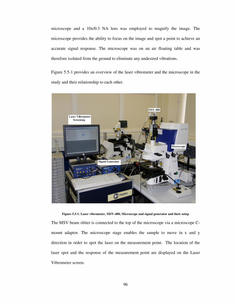
96

microscope and a 10x/0.3 NA lens was employed to magnify the image. The

microscope provides the ability to focus on the image and spot a point to achieve an

accurate signal response. The microscope was on an air floating table and was

therefore isolated from the ground to eliminate any undesired vibrations.

Figure 5.5-1 provides an overview of the laser vibrometer and the microscope in the

study and their relationship to each other.

Figure 5.5-1. Laser vibrometer, MSV-400, Microscope and signal generator and their setup

The MSV beam slitter is connected to the top of the microscope via a microscope C-

mount adaptor. The microscope stage enables the sample to move in x and y

direction in order to spot the laser on the measurement point. The location of the

laser spot and the response of the measurement point are displayed on the Laser

Vibrometer screen.

97

5.6 Custom Built Test Bed

The cochlea is located within the tympanic bone of the skull. To enable

measurements under a microscope the cochlea had to be extracted prior to the

measurements. To provide a similar environment, throughout experiments for this

work, the cochlea was fixed into a custom built, plastic test bed using two screws on

the sides. The screws ensured that the cochlea remained stationary during the

measurement process and avoid the undesired movement of the whole structure as

supposed to endosteal membrane. Care was taken that the sides of the test bed were

strong enough to hold an applied vertical force on the cochlea. Figure 5.6-1 shows

the cochlea is fixed into the test bed using the two metallic screws and the bed is

slide into the microscope stage.

Figure 5.6-1. Cochlea fixed into a custom made test bed under the microscope objective lens

The test bed was modelled using SolidWorks program and manufactured by

selective laser sintering. Selective laser sintering is an additive rapid manufacturing

technique that uses a high power laser of carbon dioxide laser to fuse small particles

of plastic, metal, or ceramic powders into a mass representing a desired 3-

dimensional object [159]. Figure 5.6-2 illustrates the cochlea test bed created by

SolidWorks.

98

Figure 5.6-2. Cochlea test bed created by SolidWorks

5.7 Preloaded Piezo Actuator

For the investigation of the cochlea frequency map, it was necessary to stimulate the

stapes head in order to simulate the natural transmission of sound vibrations into the

cochlea. Therefore a PI P-820.10 piezo actuator was employed to excite the stapes.

The P-820.10 piezo translator is a high resolution linear actuator for static and

dynamic applications. It provides up to 15 µm displacement at 0 -Y 100 G and

0.15 O# resolution. The piezo actuator can be set at a position with up to 20 m()

frequency. Figure 5.7-1 shows the P-820.10 used in the study. As can be seen, a

custom made tip with a diameter of 1 mm is attached to the piezo actuator, so it can

be positioned on the stapes head.

Figure 5.7-1. Piezo actuator attached to the custom made tip

99

5.8 Junction Box

The piezo actuator was required to excite the stapes at different frequency ranges.

Therefore it was connected to a Polytec MMA-400 Junction Box. An electrical

junction box is a container for electrical junctions, usually intended to conceal them

from sight and to some extent to eliminate tampering. It Connects the Vibrometer

controller and Data Management System and provides the piezo driver for the

scanner and amplifier for excitation signals.

The signal can be set in different forms such as; sinusoidal, pseudo random, and also

at different voltage input. For this study a periodic chirp input signal was chosen

because it has a uniform distribution of energy across the frequency range. Figure

5.5-1 represents the position of the MMA-400 Junction Box in respect to the rest of

the experimental apertures.

5.9 Eppendorf Transformer

In this study the TransformerMan NK 2 was used in order to hold the piezo actuator

at its desired positions throughout the experiments. The Eppendorf transformer

micromanipulator is designed especially for operations requiring proportional

movement of the tool.

Figure 5.9-1. Eppendorf transformerMan NK 2

100

The tool directly follows the motion of the joystick (Figure 5.9-2). This feature was

mainly used for insertion experiment to locate the electrode tip by the RW and

perform the insertion, at various speeds. The motion of the tool can be selected as

either fine or coarse and the tool can move in all three spatial coordinates (X, Y, Z).

Another feature of the system is the ability to store and select the tool position.

Storing and selecting tow position was used in the insertion experiment to locate and

relocate the electrode.

Figure 5.9-2, joystick and controller of the Eppendorf transformer

5.10 Proof of Concept

The results obtained through the proposed experimental rig raise the question of how

much the disturbances of the endosteal membrane are affected by the vibration of the

cochlea as whole. This experiment was designed to investigate the comparison of the

frequency response of the cochlea endosteal membrane exposed at a TW and the

cochlea bone, when the stapes head is excited by an actuator at 25 kHz. The results

of this experiment provide a proof for the concept of the rig and enable us to observe

how distinguished the membrane response is in contrast to the response of the

cochlea bone.

101

A 1mm TW was created on the porcine cochlea by the robotic micro-drill. The

metallic paint was placed on the endosteal membrane at the TW and its surrounding

bone. Figure 5.10-1 shows the location of the metallic paint on the TW endosteal

membrane and the surrounding bone.

Figure 5.10-1. Metallic paint on the cochlea membrane and bone

The P-820.10 piezo actuator was used to excite the stapes of the porcine cochlea at

25 kHz generated by the Polytec MMA-400 housing. The actuator was loaded on the

Eppendorf transformerMan NK 2, and it was set precisely on the stapes head. The

MSV-400-M2 MSV was employed to measure the resultant frequency data. Figure

5.10-2 shows the cochlea placed on the microscope lens and the actuator’s tip is

located on the stapes head.

Figure 5.10-2. Cochlea on the microscope lens

102

Figure 5.10-3 represents a comparison of the frequency response of the cochlea

membrane with the response of its surrounding bone. The blue line represents the

response of the endosteal membrane and the red line is the bone response during the

excitation of the stapes excitation at 25 kHz.

Figure 5.10-3. Comparison of the membrane response and bone response

As can be observed from the Figure 5.10-3, the frequency response of the cochlea

membrane is approximately 400-450 µm/s at the 25 kHz, whereas the frequency

response of the cochlea bone is approximately 5 times less at 70- 80 µm/s. The figure

also shows no significant response for the rest of the frequency range.

It can be concluded that the frequency response on the cochlea membrane is genuine

and not much affected by the vibration of cochlea as a whole, when stapes is excited

by the piezo actuator. This demonstrates the capability of the current equipment to

conduct further mapping trials.

103


The aim of this chapter was to demonstrate the general methodology used in this

study and to describe the main tools involved. At the end of this chapter the

feasibility of the experimental rig was investigated. The result of the experiment

proved that the rig is able to measure the disturbances of the endosteal membrane,

and this response is not the same as the whole structure.

The main points, which were reviewed in this chapter:

• In order to create a TW, the surgical robotic micro-drill was used to create a

hole on the cochlea; and preserve the endosteal membrane undamaged.

• The Microscope Scanning Vibrometer makes it possible to measure the

response of the endosteal membrane through a microscope.

• The response of the endosteal membrane in comparison to the vibration of

the cochlea structure is a means to prove that the results are sound.

The next chapter will demonstrate the use of the proposed experimental rig for the

third window measurements and third window excitation studies.

104

Chapter 6. Verification of Cochlear Behaviour

The aim of this chapter is to investigate disturbances within the cochlea

corresponding to the sound vibration. This chapter consists of two sections:

Section 6.1. Third Window (TW) Measurement: In the first part of this chapter

TW measurement along the path of the cochlea is described. The measurement is

based on the experimental rig introduced in chapter 5 (Methodology and

experimental tools). This is for the first time that the micro-actuation of cochlea and

measurement of disturbances within the closed bone structure of the cochlea are

combined. The results enabled the construction of a frequency response map along

the path of the cochlea.

Section 6.2. Third window Excitation: In the second part of this chapter the TW

excitation study is described. For this study the cochlea is excited at a TW on the

bony wall of the cochlea and its effect on the dynamics of cochlea are contrasted

with that of stapes excitation.

The principal outcome of the verification is to evaluate the possibility of locating an

implant actuator directly on the cochlea. Placing the implant on a location closer to

the sensitive inner ear hearing organ is expected to lead to lower energy dissipation

away from the hearing path. This will reduce the power consumed and reduce the

size of the implant in comparison with the current middle ear implant. The current

performance of the middle ear implant is reviewed thoroughly in chapter 3

(Literature review).

In chapter 4, a mathematical model of the passive cochlea was developed to help

with the understanding of the mechanism of the cochlea. At the end of each section

105

of this chapter the empirical results gathered from experiments, are used to verify the

results of the mathematical model.

6.1 Third Window Measurement

The detailed preparation of porcine cochlea as the test phantom is described in detail

in section 4.5. In this study each TW was created on a different cochlea and the

experiment was repeated three times for each of the three measurement points, and

therefore a total of 9 porcine cochlea were used at this stage.

Figure 6.1-1 represents the schematic diagram of the TW measurement experiment.

As can be observed, the piezo actuator stimulates the stapes at the oval window and

the corresponding disturbances at the TW are measured by Micro-Scanning Laser

Vibrometer (MSV).

Figure 6.1-1. Schematic diagram of TW measurement

For this measurement a TW was created by the robotic micro-drill at three points of

interest for measurement along the cochlea axis. Each TW was produced by a

drilling process under a surgical microscope. This ensured exact location for drilling.

106

The exposed endosteal membrane at the TW was found to be intact after each TW

formation. Figure 6.1-2, represents the location of the measurement points. The TWs

are located on the basal end (TW 1), next to the round window (TW 2) and the apical

end (TW 3).

Figure 6.1-2. TW measurement points

A digital calliper was used to measure the location of the TW in relation to the stapes

(S) and round window (RW). Figure 6.1-3 illustrates the location of the TWs in

terms of distance from the RW and stapes. TW 1 was created 3.10 mm anterior to the

RW and 1.97 mm from the stapes. TW 2 was created 1.78 mm anterior to the RW

and 4.45 mm from the stapes and TW 3 was created 3.77 anterior to the RW and

4.92 mm from the stapes. Then 0.01 #' of silver metallic paint was applied on the

membrane as a reflection target to be focused on by the MSV.

Figure 6.1-3. TWs in relation to RW and stapes

107

The MSV-400 scan-head was attached to the top port of the Axio plan 2 microscope

stand with a reflective filter on it. The cochlea was subsequently fixed into the

custom built test bed. Then using two screws on the sides, the cochlea remained

stationary during the experiment. The test bed was then mounted on the microscope

such that the TW was at the top of the cochlea test bed and facing the lens of the

microscope as shown in Figure 6.1-4. The laser spot from the MSV was focused

onto surface of the metallic paint at the measurement point, through the Zeiss

10x/0.3 NA lens of the microscope.

Figure 6.1-4. Cochlea under the microscope objective lens

To stimulate the cochlea at the stapes, the P-820.10 piezo actuator was used. The

actuator was loaded on the Eppendorf transformerMan NK 2 micro positioning

system. TransformerMan NK 2 enabled micro movement of the actuation, so the tip

of the actuator could be precisely located at the tip of the stapes. The correct fixture

of the actuator in relation to the stapes head was inspected using a pair of surgical

loupes (SurgiTel EV250).

The piezo actuator was connected to a Polytec MMA-400 signal generator to

generate excitation at the desired frequency range and power input. In a recent

108

assessment of the movement of the stapes by Huber [160], it was concluded that the

highest displacement peak of the stapes is approximately 2 nm, when it is subjected

to a frequency range of 500-8000 HZ of sound through the ear canal. Therefore to

optimise the results of the experiment, the power input of the piezo actuator was

adjusted to 2 G so the displacement of the actuator head is approximately 2 O# as

well. A periodic chirp input signal was chosen as it has a uniform distribution of

energy across the frequency range.

Following logging, the disturbance was presented in the Laplace domain with the

setting of 100 ##/�/G, 3200 lines JJZ� and then exported to a text file as a MSV

feature. The data was then processed using the signal processing toolbox of Matlab.

Next the results of the study are presented.

6.1.1 Results

To illustrate the response of the cochlea at different locations, in Figure 6.1-5 the

velocity amplitude of the endosteal membrane at the TW is plotted as a function of

frequency. Disturbances of the EM plotted at the three TWs created on the apex

(blue line), near stapes (red line) and near the RW (green line) provide contrast in the

response. Figure 6.1-6 represents the magnified endosteal membrane response at

each TW on a separate graph. To investigate the cochlea response to the low

frequencies, Figure 6.1-7 represents the disturbances of the EM at the three locations

of the apex (blue line), near stapes (red line) and near the RW (green line) for the

low frequency range of 0 to 1000 Hz. The remaining trials for the TW measurement

are presented in Appendix B.

Figure 6.1-5 shows that the disturbances of the endosteal membrane at the apex and

near the RW area are negligible, in comparison to the high amplitude of the

109

disturbances at the TW close to the stapes. The amplitudes at this point reach up to

approximately 1.6 0 10hf p̀ �I at 4100 and 7800 Hz. The high amplitude of the

response at the TW close to the stapes could be due to the close distance of this point

to the source of excitation. Because of the anatomy of the ear, the cochlear fluid

travels from stapes at the scala vestibule, to the RW at scala tympani. Therefore the

fluid pressure is higher at the scala vestibuli and causes more disturbances on the

EM.

Figure 6.1-5. TW measurements on cochlea

As can be observed from Figure 6.1-6, where the response at each point is plotted

separately, the basal end of the cochlea, which includes the stapes and the RW is

most sensitive to high frequencies and the highest response at the apical end is

visible at the lower frequency regions.

110

Figure 6.1-6. TW measurements of cochlea

As can be observed from the study of the cochlea response to low frequencies shown

in Figure 6.1-7, although the TW near the stapes has a gradual increase of amplitude

toward the high frequencies, the apical end of the cochlea has the greatest amplitude

corresponding to the low frequencies up to 1000 Hz.

111

Figure 6.1-7. Low frequency response of the cochlea

6.1.1.1 Results verification

Two steps were taken to verify the results of this experiment. The first verification of

the results is regarding the frequency range used in this study and the second

verification is to investigate the effect of TW measurement on different cochlea.

All results in this experiment were plotted in a frequency range of 0 to 8000 Hz as it

is the principal hearing range for human [26]. However the full frequency range of

human hearing is 0 to 20 kHz. Figure 6.1-8 provides a comparison in the

disturbances of the EM at the apex, near the RW and near the stapes for a frequency

range of 0 to 20000 Hz. This graph gives a broader picture of the endosteal

membrane’s behaviour at different locations. As can be seen from the Figure 6.1-8

the two TWs at the basal end (near the stapes and RW) are most sensitive to the

higher frequency range of 7 to 10 kHz and the TW on the apex has its greatest

amplitude at lower frequencies of 1 to 2 kHz. There is not a significant disturbance

after 11 kHz on the EM for areas away from the basal end for all the three points.

112


So far each TW measurement has been performed on different cochlea. To verify

the results three TWs were created on one cochlea, at three locations of near stapes

(TW 1), near RW (TW 2) and on the apex (TW 3) as shown in Figure 6.1-9.

Figure 6.1-9. Three TWs on the same cochlea

Figure 6.1-10 demonstrates the response of the endosteal membrane at three TWs

created near the stapes, near the RW and on the apex of the same cochlea as a

function of frequency against velocity squared. The results show a similar trend to

113

the results of the previous TW measurements, where each cochlea was created on a

different cochlea. The basal end of the cochlea is more sensitive to the high

frequencies and the apical end has its greatest amplitude at the low frequency range.

Also similar to previous results, the magnitude of the velocity amplitude is higher at

the TW near the stapes in comparison to the response at the apex and the RW.


These results show that the study of TW measurement on separate cochlea at each

location of cochlea is acceptable. The magnitude of the disturbances is almost half

than when it was a single TW on the cochlea. This demonstrates that creating a TW

effects the dynamics of the cochlea.

114

6.1.2 Verification of mathematical model

For the mathematical model of chapter 4, the TW measurement was performed on an

uncoiled cochlea. However the experimental measurement focused on the naturally

coiled porcine cochlea. The investigation was on three locations: near to the stapes,

on the apex and at the middle position along the cochlea. Figure 6.1-11 illustrates the

approximation of the location of the TWs in the mathematical and experimental

model. In the mathematical model the TWs were created at near stapes (2 mm-3

mm), on the middle (15 mm-16 mm) and on apex (30 mm-31 mm) of the uncoiled

cochlea. To verify the results the TW near the stapes was created 3.10 mm anterior

to the RW and 1.97 mm from the stapes, TW on the middle was created 2.83 mm

anterior to the RW and 3.37 mm from the stapes and TW on the apex was created

3.77 anterior to the RW and 4.92 mm from the stapes on the coiled cochlea.

Figure 6.1-11. Location of the TWs in the mathematical and experimental model.

115

Figure 6.1-12 demonstrates the predicted displacement of the endosteal membrane

(EM) gathered from the mathematical model. The blue, green and the red lines

represent 1, 4 and 8 kHz in consecutive order.

Figure 6.1-12. Predicted displacement of exposed EM at base, middle and apex of the cochlea

As can be observed from the results, the highest response at the basal end is for high

frequencies, at the middle of the cochlea is for middle frequencies and at the apical

end is for the low frequencies.

The experimental model also investigated the disturbances of the endosteal

membrane exposed at TWs created along the cochlea axis, in response to the stapes

excitation at a frequency bandwidth of 0-8 kHz. Figure 6.1-13 shows the velocity

amplitude the endosteal membrane exposed at three TWs near the stapes, on the apex

and on the middle of the cochlea.

116

Figure 6.1-13. Exposed endosteal membrane disturbances through a TW

As can be observed the results of the experimental and mathematical models are

consistent. The basal end of the cochlea is most sensitive to higher frequencies and

as it moves away from the stapes and toward the apical end of the cochlea, the

disturbances get more sensitive to the low frequencies. Also both models show that

the magnitude of the disturbance amplitude is highest near the base of the cochlea

and gradually decreases toward the apex.

In both mathematical and experimental models, it was found that higher frequency

sounds vibrate the membrane more near cochlear base whereas lower frequency

sounds vibrate the membrane further up toward the apical end. Therefore it can be

concluded that the displacement of the basilar membrane has a direct effect on the

overall dynamics of the cochlea in response to different frequencies.

117

The mathematical model enabled the sensitivity of creating a TW on the

displacement of the basilar membrane. The results did not show significant effect on

the BM displacement. However with the experimental model it was found that the

creation of more than one TW on the cochlea could reduce the response of the

cochlea.

For the purpose of mathematical modelling, the cochlea was assumed to be a

symmetrical single channel. The compliance offered by the RW and the resistance of

the helicotrema was neglected. With the experimental model the disturbances of the

EM at a TW adjacent to the RW was studied and the greatest disturbance amplitude

was visible at higher frequencies. These results were in agreement with the results of

the TW near the stapes but with significantly lower amplitude. To assess the

importance of presence of the helicotrema, it was observed that the TW created on

cochlear apical end, where the helicotrema is located is most sensitive to low

frequencies. This indicates that the helicotrema has significant effect on lower

frequency responses.

6.2 Third Window Excitation

In the TW excitation study, to determine the effect of excitation of the cochlea at a

TW, the cochlea was directly excited at a TW created on the bony wall of the

cochlea. The amplitude of disturbances produced within the cochlea was compared

with amplitudes produced by stapes excitation with similar disturbances found in the

normal hearing process. Figure 6.2-1 represents the schematic diagram of TW

excitation and measurement of the response. The cochlea was stimulated by the P-

820.10 piezo actuator at the TW created 2 mm anterior to the stapes and the

corresponding disturbances are measured at the RW, using the MSV.

118

Figure 6.2-1. Schematic diagram of the TW excitation

As a result of the small size of the cochlea relative to the large size of the microscope

lens aperture, it was not possible to measure the disturbances at another window

produced in the bony wall. Therefore the RW was selected as the measurement point

for this study. Selection of the RW as the measurement point enables a contrasting

study of disturbances within the cochlea with the advantage of keeping the cochlea

structure intact. Figure 6.2-2 illustrates the position of excitation in relation to the

RW and stapes. The diameter of the TW was 1 mm and the metallic paint on the RW

membrane is to provide a reflective target for MSV.

Figure 6.2-2. Measuring the disturbances on the RW

119

The P-820.10 piezo actuator was supported by the Eppendorf transformerMan NK 2

micro positioning device. The piezo actuator was connected to a Polytec MMA-400

signal generator that was adjusted to a frequency range of 0 / 8 m() periodic chirp

signal with input voltage of 2 G.

To perform this experiment, the signal generator was adjusted to a frequency range

of 0 / 8 m(). The logged disturbance was determined in the Laplace domain with

the setting of 100 ##/�/G, 3200 lines JJZ� and subsequently exported to a text

file as a MSV feature. Following the data was then processed using the signal

processing toolbox of Matlab. The next section will show the experimental results of

this study.

6.2.1 Results

To illustrate comparison of cochlear response to stapes and TW excitation, over a

frequency range of 0 / 8 m(), the disturbances of the RW are plotted as a function

of frequency against velocity squared. Figure 6.2-3 shows the disturbance of the

RW. The red line represents RW response to the stapes excitation, and the blue line

represents RW response to the TW excitation. The graph shows a significant

increase of disturbance amplitude of the RW with TW excitation, when contrasted

with excitation at the stapes. The main difference is observed in the area of middle

frequencies of 3000-6000 Hz which at some frequencies reaches 7 0 10hqr p̀ �I,

whereas the response to stapes excitation is almost negligible in comparison. In the

high frequency range of 7000-8000 Hz the velocity amplitude increases up to 5 010hqr p̀ �I, where the response at the stapes excitation is up to 0.5 0 10 p̀ �I. Over

the low frequency region also, the response is amplified. For instance at 1500 Hz the

120

amplitude of the response at TW excitation is seven times higher in comparison to

the stapes excitation.

Figure 6.2-3. RW disturbances at the stapes (red line) and TW (blue line) excitation

6.2.2 Verification of mathematical model

Using the mathematical model of chapter 4 was investigated on the predicted basilar

membrane displacement. The cochlea was excited at a 1 mm TW at 1mm anterior to

the stapes with three frequencies of 1, 4 and 8 kHz. Figure 6.2-4 shows the predicted

displacement of the basilar membrane as a function of distance from the stapes with

the cochlea is excited at a TW. The predicted basilar membrane displacement in

response to TW excitation is plotted as a dotted line and the solid line represents the

BM displacement in response to stapes excitation. The blue, green and the red lines

represent 1, 4 and 8 kHz in respectively.

121

Figure 6.2-4. Comparison of predicted BM response to stapes and TW excitation (Dotted line = TW

excitation, solid line = Stapes excitation)

It has to be noted that in experiment, due to the closed structure of the cochlea,

specific measurement on the basilar membrane was not possible. Therefore to show

the effect of the TW excitation on cochlear dynamics, the RW was selected as the

measurement point for this study. Figure 6.2-5 represents predicted disturbances of

the RW as a function of frequency with the cochlea excited at a TW (red line). The

blue line represents RW disturbances in response to excitation at the stapes.

Figure 6.2-5. Comparison of predicted RW response to stapes and TW excitation

122

Results from both the mathematical and experimental models illustrate the effects of

excitation of the cochlea at a TW on the disturbances within the cochlea. It was

observed that in comparison to stapes excitation, the TW excitation increases

cochlear disturbances and consequently the displacement of both the basilar

membrane and RW.


In the first section of this chapter, transient disturbances along the axis of cochlea

have been illustrated. This is corresponded to the sound vibration over a frequency

bandwidth of 0-8 kHz, using the experimental TW measurement technique.

Experimental results were in agreement with predicted trends of the mathematical

model. As expected, the indications are that the greatest sensitivity of the cochlea to

higher frequencies at the basal end and lower frequencies toward the apical end.

In the second section of the study, the effect of TW cochlear excitation on the

response within the cochlea was contrasted to that of stapes excitation in normal

hearing. The study focused on the RW as the measurement point rather than the TW.

Using the mathematical model, it is shown that, similar to TW excitation, study the

response of the cochlea to TW excitation is to increase amplification.

At the outset in this chapter, one aim was to evaluate the result of locating an implant

actuator directly onto the cochlea. The results suggest that TW excitation can be used

to amplify cochlear response to support sufferers of hearing difficulties. The results

also suggest that the ideal location for optimal excitation depends on to the specific

assistive frequency band required. As expected, the results suggest that basal end

123

should ideally be used for the high frequency and apical end for the low frequency

amplification.

124

Chapter 7. The Influence of Surgical Intervention

The aim of this chapter is to assess the disturbances within the cochlea caused by

different stages of the cochlear electrode implant procedure. Methods of minimizing

trauma are suggested. Trauma during implantation is thought to diminish hearing

preservation. The movement of the endosteal membrane is a representation of the

underlying pressure changes within the cochlea as indicated in chapter 5. Therefore

high velocity amplitudes of membrane are in response to large pressure amplitudes

within the scala tympani and hence likely greater trauma.

In this chapter there are three studies to show the impact of the surgical procedures

on cochlea disturbance levels:

Section 7.1. Drilling speed and force: In this section the effect of drilling at

different speeds and applied drilling forces on the disturbances within the cochlea are

investigated.

Section 7.2. Manual and Robotic cochleostomy: In the second section of this

chapter a comparison of the disturbances within cochlea during the cochleostomy

procedure by human (manual) and force controlled robotic micro-drill is performed.

At this section the effect of the opening the endosteal membrane by a running burr

and a surgical knife is also compared.

Section 7.3. Electrode insertion: In the last section of this chapter the disturbances

of the endosteal membrane during manual electrode insertion with robotic insertion

is compared. There is also an investigation of the effect of electrode insertion speed

on the disturbances within the cochlea.

Over the past 20 years cochlear implantation has become the standard treatment for

the severe to profoundly deaf

electronic device used to treat severe

implanted underneath the skin

implantation procedure

and inserting an array of electrodes into the spiral shaped cochle

procedure involves drilling through the bony cochlea wall, approximately 1

thick, to reveal the endosteal

wall and is a thin membrane of 0.1

membrane are fluids that oscillate

has to be opened to insert the electrode array.

manually with no knowledge of its effect on the fine inner structures of the cochlea.

Figure 7-1 illustrates the insertion of the cochlea electrode array inside the cochlea

through a cochleostomy.

Figure 7-1. Insertion of the cochlea electrode through a cochleostomy

It was initially assumed that, s

residual hearing of a patient. However more recently, it has been discovered that it is

possible to perform the implantation procedure

a patient’s residual hearing.

125


to profoundly deaf patient. A cochlear implant is a small, complex

electronic device used to treat severe to profound hearing loss. It is surgically

implanted underneath the skin behind the patient’s ear. The essence of the cochlear

implantation procedure involves drilling a cochleostomy through the cochlea

and inserting an array of electrodes into the spiral shaped cochlea. The cochleostomy

involves drilling through the bony cochlea wall, approximately 1

o reveal the endosteal membrane. Underline the surface of the bony cochlea

is a thin membrane of 0.1 mm-0.2 mm thick. Under the endosteal

that oscillate in the presence of acoustic energy. The

has to be opened to insert the electrode array. The electrode array is inserted


illustrates the insertion of the cochlea electrode array inside the cochlea

through a cochleostomy.

. Insertion of the cochlea electrode through a cochleostomy [127]

It was initially assumed that, standard cochlear implantation would

patient. However more recently, it has been discovered that it is

perform the implantation procedure and retain a significant proportion of

patient’s residual hearing. As a result the concept of hearing preservatio


A cochlear implant is a small, complex

to profound hearing loss. It is surgically

The essence of the cochlear

involves drilling a cochleostomy through the cochlear bone

a. The cochleostomy

involves drilling through the bony cochlea wall, approximately 1-2 mm

nderline the surface of the bony cochlea

the endosteal

The membrane

he electrode array is inserted


illustrates the insertion of the cochlea electrode array inside the cochlea

[127]

would destroy the

patient. However more recently, it has been discovered that it is

a significant proportion of

As a result the concept of hearing preservation cochlear

126

implantation (HPCI) has become the centre of attention within the cochlear

implantation community [161]. As mentioned above formation of the cochleostomy

and insertion of the electrode are considered to be two major steps in the

implantation procedure. Therefore changes to design of electrode and surgical

techniques have been made to optimise these procedures and retain the residual

hearing of the patient.

7.1 Drilling Speed and Force

Drilling speed and force applied by the surgeon are considered to be important to

disturbance amplitude. Currently the effects of the drilling speed and force have been

left as a personal choice of the surgeon.

This experiment was designed to contrast the effect of drilling a cochleostomy at

different speeds and assessing impact on the amplitudes of disturbances within the

cochlea as sealed lumen. The velocity of movement of the endosteal membrane

during the drilling process is in response to fluid pressure changes within the scala

tympani.

7.1.1 Experimental setup

The preparation of test specimens was described earlier in section 5.2.1. A schematic

configuration of the equipment used in the experimental measurement is shown in

Figure 7.1-1.

127

Figure 7.1-1. Schematic diagram of the experimental configuration of drilling on the cochlea

A third window (TW) to the cochlea was created on the far anterior aspect of the

basal turn of the cochlea, approximately 9 mm directly anterior from the anterior lip

of the round window (RW) niche. The location of the TW in relation to the RW and

stapes is illustrated in Figure 7.1-2.

Figure 7.1-2. TW created by robotic micro-drill

Approximately 0.01#' of silver metallic paint was applied onto the endosteal

membrane as a reflective target to be focused by the Micro-Scanning Laser

Vibrometer (MSV).

128

Then the test bed was mounted on the microscope with that the TW was oriented

perpendicular to the Zeiss 10x/0.3 NA lens of the upright microscope.

The MSV-400 scan-head was attached to right-hand port of the Axio plan 2

microscope stand with reflective filter on. The laser spot from the MSV was then

focused onto surface of the metallic paint.

The disturbances induced by drilling on the surface of the cochlea are measured

using the MSV working through the microscope. Figure 7.1-3 presents a clear image

of the experimental setup of the drilling process. The red light emitted on the cochlea

surface is the laser beam of the MSV. Next drilling procedure is described in details.

Figure 7.1-3. Drilling manually on the cochlear

7.1.1.1 The drilling experiment

Trial drilling was performed manually by an experienced ENT consultant surgeon,

anterior/inferior to the RW in an area of approximately 2 0 2 ##, in the typical

position for a cochleostomy during the cochlear implant procedure using a 1mm

diamond drill burr. The relation of drilling area to the RW and TW is represented in

129

Figure 7.1-4. The actual surface of the cochlea is hemespherical, however due to the

angle and magnification of the camera the cochlea surface appears planar.

Figure 7.1-4. Trial drilling area

The drill was connected to a control box to enable measurement of the feed force

applied to the cochlea by the burr. To investigate the effect of drilling speed on

disturbance amplitude, when creating a cochleostomy, drilling was performed at four

different speeds; 20000, 10000, 5000 and 1000 rev/min, each at three different forces

of 0.5, 1.5 and 5 N for a period of 10 seconds.

At the force of approximately 0.5 N the burr was only just in contact with the

cochlea bone. At the force of approximately 5 N the surgeon was pressing hard on

the bone with the drill burr, similar to the force used while performing the cortical

mastoidectomy step of the cochlear implant surgery. Each drilling was performed on

a different cochlea, therefore a total of 12 cochlea were used.

During each trial the disturbances of the endosteal membrane at the TW was

measured by the MSV and presented in the Time domain. Following logging the

data was presented in the time domain with the setting of 100 ##/�/G, 262144

lines Z:#g� and 25.6 m() sample frequency, with a resolution of 39 1� , and then

130

exported to a text file as a MSV feature. The data was then processed using signal

processing toolbox of Matlab.

7.1.2 Results

Here to illustrate the impact of drilling at different force and speed, the velocity

amplitude of the endosteal membrane at the TW is plotted as a function of time. The

results of drilling at three different forces of 5 N, 1.5 N and 0.5 N using four

different drilling speeds of 20000, 10000, 5000 and 1000 rev/min are represented at

Figure 7.1-5, Figure 7.1-6 and Figure 7.1-7 respectively. The difference in amplitude

indicates difference at the disturbances level. Following the results, the mean value

of disturbances corresponding to each graph is presented at Figure 7.1-8. At the end

of the section, to assess the disturbances in the frequency spectrum, the results of the

drilling at 5 N were converted to frequency domain and presented in Figure 7.1-9 as

a function of frequency against velocity.

As shown in Figure 7.1-5 the maximum velocity amplitude is 1.2 m/s for all drilling

speeds at an applied feed force of 5 N. As shown in Figure 7.1-6 the peak velocity

amplitude falls to a value of 0.8 m/s with a feed force of 1.5 N. Figure 7.1-7

demonstrates relatively insignificant disturbance at drilling with an applied feed

force of 0.5 N. However as the speed increases the total amount of contact and

therefore the response reduce. This could be explained in way that in the higher

speeds it is harder to control the drill manually, and more care has to be taken in

respect to the exact location of the drilling. Consequently it will lead to a less drilling

as the speed increases.

131

Figure 7.1-5. Drilling with a force of 5N at different speeds

Figure 7.1-6. Drilling with a force of 1.5N at different speeds

132

Figure 7.1-7. Drilling with a force of 0.5 N at different speeds

The results indicate that the applied drilling force is the dominant factor in respect to

the velocity amplitude of the endosteal membrane. This is more apparent in Figure

7.1-8, where mean values of the endosteal membrane disturbances at different force

and speeds are illustrated. The blue, red and green bars represent the average

disturbances at applied drilling force of 5, 1.5 and 0.5 N respectively at each speed.

Figure 7.1-8. The mean value of the endosteal membrane disturbances at different speeds and applied

force

133

As can be observed, from Figure 7.1-8, the mean disturbances of the endosteal

membrane increases as more drilling force is applied. One important factor to

consider form the graph is the low mean value corresponding to the drilling speed of

20000 rev/min to the rest of the drilling speeds at the same force. One hypothesis to

explain this surprising finding is that at lower speeds the burr is likely to exhibit

more bounce after removing a section of bone than at high speeds when it is likely to

be smoother. This also can be that the control of the drill gets harder at higher speeds

and therefore creates more sudden contacts between the drill burr and cochlea bone

rather than a gradual drilling.

To support the hypothesis of the effect of drilling force on the disturbances within

the cochlea, a statistical test of Analysis of Variance (ANOVA) was performed

between the results of similar speed drilling but of three groups of 0.5, 1.5 and 5 N

drilling forces. The results of the test show a P-value less than 0.0001, which

suggests a statically significant difference between the results of drilling with the

same speed but different forces. This confirms the hypothesis that the applied force

factor has more impact on the disturbances created.

Figure 7.1-9 illustrates the frequency response of the TW membrane while drilling at

four speeds of 1000, 5000, 10000 and 20000 rev/min respectively at a drilling force

of 5 N in velocity as a function of frequency. It can be observed from the graph that

as the drilling speed increases the resonance frequency also raise. The lowest

resonance frequency is at drilling speed of 1000 rev/min at 160 Hz and the highest is

at the drilling speed of 20000 rev/min at 400 Hz. However the amplitude of the

disturbances remains approximately similar for all the speeds as the applied force is

the same at 5 N. The resonance frequency and their corresponding amplitude are

presented in Table 7.1-1.

134

Figure 7.1-9. Frequency spectrum of the disturbance of the cochlea in response to drilling

Table 7.1-1. Resonance frequency for each drilling speed

7.1.3 Results verification

So far each drilling was performed on a different cochlea and proved that the

corresponding disturbances are more related to the applied force rather than the

speed. To verify these results we performed a trial of drilling at three different

forces of 0.5, 1 and 5 N with a drilling speed of 10000 rev/min. Figure 7.1-10

represents the relation of the drilling force applied and corresponding disturbance.

135

The top graph represents the disturbance in velocity and the bottom graph shows the

corresponding force as a function of time.

Figure 7.1-10. The relation of the drilling force applied and corresponding disturbance.

As can be observed, the highest disturbance is observed when drilling was performed

at 5 N force, which is approximately 0.8 m/s. The graph shows, that as the force

applied on the cochlea get lower, it has a direct effect on the disturbances created

within the cochlea.

7.1.4 Discussion

The current study presents an assessment of exposed endosteal membrane

disturbance whilst drilling is performed on the cochlea. The results demonstrate that

the mean value of drilling at 5 N is approximately 1.4 times higher than 1.5 N and 5

times higher than the 0.5 N at all the four speeds. Therefore it can be concluded that

in the process of the drilling on the cochlea the applied force is a dominant effect in

respect to the disturbances within the cochlea. This study, to the author’s knowledge

136

is the first TW measurement on the effect of drilling speeds and force at the

cochleostomy formation process.

These findings raise the question of the trauma within the cochlea caused by drilling.

It is possible to assume that the increase in disturbance of the endosteal membrane

would have a detrimental effect on the low frequency threshold. This study

reinforces the concepts presented by Zou [39] that vibrational trauma is likely to be a

factor in the trauma sustained by the cochlea independent of noise induced trauma.

In one previous study by Pau [162] on noise exposure of the inner ear during drilling

a cochleostomy with drilling speed of 24000 to 27000 rev/min, the sound pressure

level (SPL) within the cochlea was examined. The results of that study showed a

clear resonance at frequency of 400 to 450 Hz corresponding to a drilling speed of

24000 to 27000 rev/min. This confirms the result of the presented work where the

corresponding resonance frequency at the drilling speed of 20000 rev/min with force

of 5 N is 400 Hz.

Pau also suggests that SPL within the cochlea is dependent on the drilling speed.

However there was no investigation on the drilling force factor used while the

drilling. The present measurement has focused on the velocity disturbance of the

endosteal membrane during the drilling only. As mentioned at chapter 5, it has been

shown that the SPL is directly related to the value of the membrane velocity G,

which is obtained by the MSV. Having found that the force applied at drilling

process have a greater impact on the membrane velocity, it can be concluded that

increase in the drilling force will result in the higher SPL within the cochlea.

Base on the findings of this study there two approaches with respect to reduce the

disturbances while drilling the cochleostomy. One approach would be to replace the

137

insertion path by the RW insertion [162, 163]. Inserting via the RW will eliminate

the risk of drilling on the cochlea and guarantees the positioning of the electrode

array in the Scala tympani. However the angle of the RW has made it less favourable

for surgeons.

The other approach will be to either perform the drilling at a controlled low force

procedure by employing robotic techniques or use some means of support for the

arm. Both approaches guarantee steady position and force regardless of the speed,

and therefore avoid a sudden contact with the cochlea surface and eliminate tremor

[164]. Using the robotic force controlled approach would also enable the surgeon

with less skill to perform the surgery.

The results of this study are only for a range of 10 seconds of drilling. A further

study is required to investigate the endosteal membrane disturbance throughout the

full cochleostomy procedure. It can be speculated that the disturbance will rise

dramatically as the drill burr touch the membrane at the time of breakthrough. Next

section will explore using a robotic force controlled micro-drill as a means to create

a cochleostomy and investigate the corresponding disturbances in contrast with

manual cochleostomy.

7.2 Manual and Robotic Cochleostomy

This experiment was designed to compare the induced vibrations within the cochlea

during formation of the cochleostomy, using the robotic micro-drill and conventional

manual drilling. There was also a comparison of the disturbances, when the

endosteal membrane at the cochleostomy was punctured by a surgical knife at the

robotic procedure or by a running burr at the manual drilling.

138

This experiment will follow the experimental setup of the previous study on the

effect of drilling speed and force the disturbances created within the cochlea. At that

study it was concluded that the applied drilling force by the surgeon is a dominant

effect in respect to the disturbances within the cochlea, and therefore a force

controlled drilling process was suggested. Further study is required to investigate the

endosteal membrane disturbance throughout the full cochleostomy procedure.

Next will describe the experimental setup of the experiment and obtained results,

followed by a discussion.


As mentioned above the experimental setup of the study is similar to the previous

experiment in section 7.1.1.

7.2.1.1 Contrasting the manual and robotic drilling process

Drilling was performed anterior inferior to the RW, in the typical position for a

cochleostomy during the cochlear implant procedure. Six cochleostomies were

performed on separate porcine cochleas, 3 in the manual group and 3 in the robotic

group.

The manual cochleostomies were performed by a skilled ENT surgeon, using a 1 mm

diamond burr at a speed of 10,000 revs/min. At completion of cochleostomy, to

assess the disturbances caused by introducing a running burr into the scala tympani,

no attempt was made to preserve the underlying endosteal membrane. The surgeon

applied a similar force of drilling to that used during human cochlear implantation,

although this force was not specifically assessed at this stage. The surgeon wore

139

wearing a pair of surgical loupes (SurgiTel EV250) to inspect the correct position of

drilling.

Figure 7.2-1 represents the experimental setup of the manual cochleostomy drilling.

The surgeon’s hand is supported by a robust arm rest to avoid any undesired hand

movement.

Figure 7.2-1. Manual cochleostomy procedure

The robotic cochleostomy was performed using the robotic micro-drill. The robotic

cochleostomies were created with preservation of the endosteal membrane inherent

with the use of this robotic drill. The same drill burr as in the manual tests was used

(1 mm diamond); at a drilling speed of 700 rev/min. Figure 7.2-2 demonstrates the

position of the drill burr with respect to the cochlea. As can be observed in the

figure, the robotic drill is being supported by a snake arm. The robotic drilling arm

was manoeuvred into the precise location for cochleostomy drilling by the surgeon.

The setup time for the robotic drill was approximately 2 minutes. The direction and

140

angle of drilling achieved through the posterior tympanotomy was similar to that of a

conventional cochleostomy formation, with an adequate view of the drilling site.

Figure 7.2-2. Robotic cochleostomy drilling

Figure 7.2-3 represents the measurement setup at the robotic cochleostomy

procedure. As can be seen the drill is supported by snake arm attached to a fixed

table and the measurement is performed by the MSV. The force and torque transients

are also monitored during the drilling process.

Figure 7.2-3. Robotic cochleostomy measurements setup

141

The axial drill force was limited to 2 N to ensure that the underlying membrane was

not perforated when the burr drilled through the cochlear bone. Irrigation was used

throughout all drilling procedures.

Figure 7.2-4 is the graphical representation of the force (red line) and torque (blue

line) experienced by the drill. Both respiration and the heart rate can be determined

from the traces, demonstrating the sensitivity of the drill. The robotic drilling

consists of two stages.

• Contact (0-8 s); Drill is placed on trajectory for cochleostomy by the surgeon.

The drill is advanced and when contact is detected the drill feed stops.

• Drilling (10-105 s): There is a gradual rise in the force and torque until the

105th

seconds where there is sudden drop in force and raise in torque. At this

point the drill automatically detects the breakthrough of the bone and stops.

Figure 7.2-4. Graphical representation of the force and torque at robotic drilling

142

The slight force drop at 77th

seconds is as the result of irrigation of the drilling area.

However as there is no raise in torque the drilling process is not halted and still

continues.

Following logging, the data was presented in the time domain with the setting of

100 ##/�/G, 262144 lines Z:#g� and 1.28 m() sample frequency, with a

resolution of 781 1� , and then exported to a text file as a MSV feature. The data

was then processed using signal processing toolbox of Matlab.

7.2.2 Results

Here to compare the disturbances generated by the manual and robotic

cochleostomies, the vibrations of the endosteal membrane at the TW were plotted as

a function of time against velocity. The result of the manual drilling is presented at

Figure 7.2-5 and the robotic drilling at Figure 7.2-6. To make better judgment on

comparison the results of the manual and robotic drilling are plotted in the same

scale at Figure 7.2-7. Following the results, the mean value of disturbances

corresponding to each graph is illustrated at Figure 7.2-8

As can be observed from Figure 7.2-5, the maximum velocity amplitude for the

manual drilling is approximately 1 m/s. The membrane breakthrough (BT) points,

when the drill burr breaks through the membrane are indicated in the graph. The

process of breakthrough with a running burr into the scala tympani did not appear to

be any more traumatic than the manual drilling process itself. The first trial was

finished in 23 s, and was very short compared to the second and third trial which

were 71 and 73 seconds. The gaps on the graph are resulted as the surgeon had to

remove the drill and irrigate the drilling area.

143

Figure 7.2-5. Disturbance of the endosteal membrane at manual cochleostomy

The effect of the robotic drilling on the disturbances of the endosteal membrane is

demonstrated in Figure 7.2-6. The measurement was taken in a range of 250, but the

finishing time varies for each cochlea. The first trial took approximately 200 seconds

and the second and third trial took 170 and 140 seconds to complete. In all three

trials the robotic drilling process preserved the endosteal membrane, which was

tested by visual inspection and palpitation of the membrane. Drill breakthrough of

the cochlear bone was detected and controlled within 15 µm of the bone surface. The

bony cochleostomy was approximately 0.8 mm in diameter.

144

Figure 7.2-6. Disturbance of the endosteal membrane at Robotic cochleostomy.

As shown in Figure 7.2-7 the disturbances of the endosteal membrane are

significantly reduced by robotic drilling compared to the manual drilling. Robotic

drilling also demonstrates a uniform disturbance during the process of drilling

whereas in the manual drilling process there are signs of impact with each sweep of

the surgical drill.

Figure 7.2-7. Disturbance of the endosteal membrane at manual and robotic procedure

145

As can be observed from Figure 7.2-8, the mean membrane velocity during the

robotic drilling is 4% of the velocity when it is drilled manually. Furthermore, the

peak membrane velocity during the robotic cochleostomy is 1% of the velocity

observed during manual drilling.

Figure 7.2-8. The mean value of the disturbance at manual and robotic cochleostomy

The results of the t-test demonstrated that the two-tailed P value is less than 0.0001,

between the responses at the robotic and manual drilling and by conventional criteria

this difference is considered to be extremely statistically significant.

7.2.3 Opening the membrane

At the manual procedure the membrane was punctured by the running burr during

the drilling process and the break through caused disturbance velocity of up to 1 m/s.

However at the robotic drilling the break though was controlled and drilling

automatically stopped prior to the break through. Subsequent the robotic micro-drill

stopped, the integrity of the endosteal membrane was assessed. Upon confirmation

of the unbroken membrane, it was punctured with a surgical pick. In a cochlear

implantation procedure, the electrode array would be inserted through this hole into

146

the scala tympani. The opening of the membrane was also by the experienced ENT

surgeon, while wearing a pair of surgical loupes (SurgiTel EV250). As can be seen

in Figure 7.2-9 the surgeon’s hand was rested on a fixed support, in order to

minimise unwanted hand tremor.

Figure 7.2-9. Surgeon puncturing the endosteal membrane using a pick.

Figure 7.2-10 represents the disturbances of the endosteal membrane during to the

puncturing at the cochleostomy in velocity as a function of time. The whole process

took approximately 10 second to complete and was performed on three

cochleostomies created by the robotic micro-drill.

Figure 7.2-10. Endosteal membrane movement at opening of cochleostomy by needle

147

As can be observed, opening the membrane with a pick resulted in no discernable

membrane movement on 2 occasions and a 0.02m/s disturbance on one occasion.

Bone fragments on the endosteal membrane required removal prior to opening of the

membrane. The statistical student t-test between the disturbances created by

puncturing of the membrane by a surgical pick and the running burr suggested a P

value is less than 0.0001, where is considered to be extremely statistically

significant. Even in case with the highest peak at 0.2 the disturbance is 50 times less

than the manual break through.

7.2.4 Discussion

This study contrasts the measurements of endosteal membrane disturbance during

manual and robotic cochleostomy formation. It was concluded from the results that

using the robotic micro-drill the mean membrane velocity during the robotic drilling

is 4% of the velocity when it is drilled manually.

Whilst there was an expectation for the robotic micro-drill to cause lower

disturbance level to the cochlea, the difference was not anticipated to be quite so

significant. These findings may have implications for drilling technique. Due to

limiting the force, the robotic micro-drill is able to ensure that a constant force is

applied from the burr to the bone at all times. This is achieved by controlling the

linear displacement of the robot where the drill advances or withdraws in response to

the feedback depending on drilling characteristics. Manual drilling usually involves

impact onto the bone, one with each sweep of the bone surface. On each sweep, the

burr will move away from the bone, but will also rebound, leading to an increase in

the force applied into the bone. As bone is removed, the forces continually change

and these forces are well below the range of a human’s ability to sense and control.

148

A further factor is the angle of drilling. Figure 7.2-11 shows the drilling angle in

manual and robotic drilling. In manual drilling, the burr is held at a slight angle so

that the surgeon has a view of the target area to avoid inadvertent penetration of the

underlying membrane. Irrigation is constantly performed through to the tip of the

burr and often, the surgeon must remove the burr to allow the liquid to be suctioned

out and the drilling site to be inspected. The inspection assesses the integrity

endosteal membrane. The sweep of the drill burr and the impact of the tip after each

inspection are the major factors leading to spikes in the force delivered to the cochlea

during manual drilling. However in the robotic drilling, the burr is held

perpendicular to the drilling site. The burr is constantly irrigated with no need of the

burr to be moved from the target area.

Figure 7.2-11. Drilling angle in manual and robotic drilling

The most important aspect of the robotic cochleostomy is breakthrough detection.

This feature allows the bone drilling process to stop just before the membrane is

reached, resulting in the preservation of the endosteal membrane. Lenhardt [133]

recommends the ideal way to minimize trauma during cochleostomy formation is to

perform a bony cochleostomy preserving the underlying endosteal membrane. In this

method the membrane is subsequently opened with a pick/knife rather than a running

149

burr in manual drilling method. This method avoids introducing a running burr into

the scala tympani. A previous study by Pau has shown that the highest SPL within

the cochlea is when a running burr touches the endosteal membrane [162]. Further

the disturbances within the cochlea whilst opening the membrane with a surgical

pick is shown minimal.

Figure 7.2-12 represents the manual (left) and the robotic (right) cochleostomy. As

can be seen the robotic cochleostomy is much neater than the manual one and there

is no effect of the drill debris on the cochlea.

Figure 7.2-12. Manual and robotic cochleostomy

7.3 Electrode Insertion

In this experiment the aim was to determine two important factors during insertion of

a cochlear implant electrode array. The first is to investigate the effect of insertion

speed on the disturbances of the endosteal membrane. The second aim is a study

contrasting the disturbances during manually (current procedure) and robotic

electrode array insertion. Minimizing the trauma sustained by the cochlea during

insertion is thought to be a critical feature in hearing preservation cochlear

implantation [165].

Last section investigated the effect of different methods of cochleostomy formation.

Following cochleostomy formation the electrode array is inserted into the scala

150

tympani of the cochlea. This is currently performed manually by the surgeon. The

quality of hearing result post cochlear implantation is dependent on preservation of

cochlear anatomy during insertion plus achieving a full insertion of the electrode

array deep into the spiral cochlea. Membrane rupture forces are below the threshold

detectable by human hands. Recently there have been proposals for automated

cochlear implant tool [138]. However there is no knowledge of the disturbances

created during manual or the robotic methods of insertion.


The preparation of test specimens is described in detail in section 5.2.1. Using the

robotic micro-drill a TW was created on the far anterior aspect of the basal turn of

the cochlea, approximately 2.80 mm anterior to the anterior lip of the RW and 4.90

mm anterior to the stapes. The size of the TW was chosen 2 mm to provide an

adequate area for membrane movement. Approximately 0.02 #' of silver metallic

paint was applied onto the intact endosteal membrane. Figure 7.3-1 illustrates the

relation of the TW in respect to the RW and stapes (S). The metallic paint is visible

at the TW.

Figure 7.3-1. The TW created for insertion measurements

151

An opening was created in the RW membrane using a pick, through which the

electrode array could be inserted. The process was performed under a surgical

microscope. Figure 7.3-2 demonstrates the process of puncturing the RW by a pick.

Figure 7.3-2. Creating a hole in the RW using a surgical pick

Figure 7.3-3 shows the completed opening in the RW.

Figure 7.3-3. The arrow indicates the insertion location in the RW

The schematic of the configuration equipment used in experimental measurement is

shown in Figure 7.3-4. The electrode is inserted via the opening at the RW and the

corresponding disturbances are measured at the TW, by the MSV through the

microscope.

152

Figure 7.3-4. Schematic diagram of the experimental configuration

7.3.1.1 Contrasting the manual and robotic insertion procedure

A MED-EL cochlear implant electrode was used for this study. The MED-EL

electrode array has no stylet and is a soft, flexible electrode; it is inserted into the

cochlea by simple advancement. The array was inserted to a depth of 15 mm, first

manually and then using a robot at three different speeds.

Figure 7.3-5 illustrates the experimental setup at the manual electrode insertion. The

manual insertion was performed by an experienced ENT surgeon. The surgeon rested

his hand on an arm support to minimise the hand tremor [164] and pushed the

electrode array inside the cochlea through the hole created in the RW. The correct

fixture of the electrode in relation to the insertion location and the insertion process

was inspected using a pair of surgical loupes (SurgiTel EV250). The laser beam on

the TW from the MSV is visible in the Figure 7.3-5.

153

Figure 7.3-5. Manual insertion of the electrode array

The robotic insertion was accomplished by a micro positioning Eppendorf

transformerMan NK 2. Using the Eppendorf transformerMan the electrode was

placed at the opening in the RW and subsequently inserted robotically. Micro

positioning system was set at different speeds of 500, 3000 �OB 7000 tp̀ to

advance the electrode for 15 mm. As can be seen in Figure 7.3-6 the MED_EL

cochlea electrode is taped to the micro positioning system

Figure 7.3-6. MED_EL cochlea electrode, taped to the micro positioning system

Figure 7.3-7 shows the robotic insertion of the electrode into the cochlea using a

Eppendorf micro positioning system under the microscope.

154

Figure 7.3-7. Robotic insertion of the cochlea electrode

During each insertion trial, the disturbances of the endosteal membrane at the TW

were measured by the MSV and presented in the time domain. Following logging the

data was presented in the time domain with the setting of 100 ##/�/G, 65536 lines

Z:#g� and 2.56 m() sample frequency, with a resolution of 390 1� , and then

exported to a text file as a MSV feature. The data was then processed using signal

processing toolbox of Matlab.

7.3.2 Results

The results of the study are presented in two parts. At first part the effect of the

insertional speed on the disturbances within the cochlea and at the second part a

comparison between the robotic and manual method was performed.

7.3.2.1 Robotic insertion at different speeds

The results of robotic insertion at three speeds of 7000 tp̀ , 3000 tp̀ and 500 tp̀

are represented at Figure 7.3-8, Figure 7.3-9 and Figure 7.3-10 respectively as a

function of frequency against velocity. The difference in amplitude indicates

difference at the disturbances level. Three trials are plotter for each speed. The mean

value of disturbances corresponding to each graph is then presented at Figure 7.3-11.

155

The first three figures show insignificant disturbances all along the range, with

occasional peaks. The highest peak reaches up to 10 tp̀ , 9 tp̀ and 8 tp̀ at Figure

7.3-8, Figure 7.3-9 and Figure 7.3-10 respectively.

Figure 7.3-8. Disturbances of endosteal membrane at robotic electrode insertion at a speed of uvvv wec

Figure 7.3-9. Disturbances of endosteal membrane at robotic electrode insertion at a speed of xvvv wec

156

Figure 7.3-10. Disturbances of endosteal membrane at robotic electrode insertion at a speed of 5vv wec

It is difficult to distinguish between the results of the disturbances corresponding at

different speed in robotic insertion. Therefore to make a more clear comparison the

mean value of the disturbances at each speed has been determined at Figure 7.3-11.

As can be observed from the figure, the average disturbance is directly related to the

insertional speed, in other word, the increase of insertion speed will raise the average

disturbance. The highest average disturbance is at insertion speed of 7000 tp̀ ,

which is approximately 0.7 tp̀ and the lowest is for 500 tp̀ insertion speed, where

is 0.18 tp̀ .

157

Figure 7.3-11. Average disturbance at three different speeds of robotic insertion

To support the hypothesis of the effect of insertion speed on the disturbances within

the cochlea, a statistical test of Analysis Of Variance (ANOVA) was performed

between the results of for insertion at three different speeds

of 500, 3000 �OB 7000 tp̀ . The results of the test show a P-value less than 0.0001,

which suggests a statically significant difference between the results of insertion at

different speeds. This confirms the hypothesis that the insertion speed factor has a

direct impact on the disturbances created.

7.3.2.2 Robotic and manual insertion

At this part of the study the disturbances of the endosteal membrane are compared at

the manual and robotic insertion. Therefore the disturbances of the endosteal

membrane at the TW are plotted as a function of time against velocity for each

method. The result of the manual insertion is presented at Figure 7.3-12 and the

robotic insertion at Figure 7.3-13. To make a better judgment on comparison the

results of the manual and robotic insertion are plotted in the same scale at Figure

7.3-14. Following the results, the mean value of disturbances corresponding to each

graph is illustrated at Figure 7.3-15.

0.00E+00

1.00E-07

2.00E-07

3.00E-07

4.00E-07

5.00E-07

6.00E-07

7.00E-07

8.00E-07

1 2 3

Ve

loci

ty (

m/s

)

7000 μm/s

3000 μm/s

500 μm/s

158

As can be observed from Figure 7.3-12, the first and second trials have a uniform

behaviour (no sudden peak) during the insertion and major disturbances are visible,

when the electrode is moving inside the scala from 1.5 s to 3 s. The amplitude at

these two graphs reaches up to 0.5 tp̀ . However there are two main peaks visible in

the last trial. The first peak is at the point of the entrance of the electrode inside the

cochlea at 0.5 s and the second peak is the point where the electrode reaches the end

of the scala. The highest amplitude at this graph is 1.5 tp̀ .

Figure 7.3-12. Disturbances of Endosteal membrane at manual insertion

To represents the results of the robotic insertion the average disturbances of three

trials corresponding at each insertion speed was plotted. As can be seen from the

Figure 7.3-13 there is no significant disturbances notable at any tail.

159

Figure 7.3-13. Average of disturbances of endosteal membrane at robotic insertion

Figure 7.3-14 provides a comparison of the disturbances within the cochlea at the

robotic and manual insertion. As can be observed from the graph, the results of the

robotic insertion are more uniform than the manual insertion, where occasional peaks

are visible due to the hand movement of the surgeon or uneven applied force and

speed while inserting the electrode.

Figure 7.3-14. Comparison of the disturbances at manual and robotic insertion.

160

Figure 7.3-15 presents the average disturbances of the robotic insertion at three

speeds and manual insertion. As shown in the graph the highest disturbance is at the

manual insertion at approximately 38.2 tp̀ , which is only 0.4 tp̀ higher than the

insertion at 7000 tp̀ . However the gap is significantly higher between the manual

and robotic insertion at 500 tp̀ where it reaches 3.7 tp̀ .

Figure 7.3-15. Comparison of average of the disturbances at manual and robotic insertion

To have a more optimal contrast between two methods, a statistical student t-test was

performed between the manual insertion and each robotic insertion speed. The

results of the t-test demonstrated that the two-tailed P value is less than 0.0001,

between the robotic insertion at speeds of 500 and 3000

tp̀ and the manual insertion.

By conventional criteria, this difference is considered to be extremely statistically

significant. However the P-value equalled 0.3975 at the test between the robotic

insertion at speed of 7000 tp̀ and the manual insertion, which means this difference,

is considered to be not statistically significant.

0.032

0.033

0.034

0.035

0.036

0.037

0.038

0.039

Ve

loci

ty (

mm

/s)

Manual and Robotic Insertion

500 μm/s

3000 μm/s

7000 μm/s

Hand Insertion

161

7.3.3 Discussion

The first aim of this study was to determine the effect of the speed of insertion on the

overall disturbances of the endosteal. It was concluded that increasing electrode

array insertion speeds leads to greater disturbances within the cochlea during the

insertion process. The fact that a slower robotic insertion speed leads to less

endosteal membrane disturbance makes logical sense, interestingly the difference

between the different speeds is very small.

The second aim of the study was to compare the endosteal membrane disturbances,

during robotic and manual hand insertions. Therefore it was concluded that robotic

insertion leads to lower disturbances of the endosteal membrane than manual

insertion. However, when the speed of the robotic insertion reached 7000 tp̀ , the

disturbances were similar to the manual insertion. Robotic insertion would be

expected to be less traumatic than manual insertion due to the constant speed of

insertion.

So far the design of electrodes for cochlear implant and the depth of insertion has

been the focus of research for many decades [136, 166, 167]. To the author’s

knowledge this study is the first attempt to contrast the intracochlear disturbances

using different methods of the electrode insertion.

In a study by Donnely [168] the Effect of cochlear implant electrode insertion on

stapes function was measured by intra-operative Laser Doppler Vibrometry. It was

concluded that insertion of a cochlear implant electrode produces a change in stapes

displacement at low frequencies. The results coincides with the results of this study

as the most significant disturbances within the cochlea at insertion was observed at

low frequency range of 0 to 400 ().

162

There was no assessment on the insertion speed at the manual method. Previous

research by Schurzig [169] has shown an average insertion speed of 3000 tp̀ at

manual insertion. However in the present study the disturbances corresponding the

manual insertion were closer to the results of the insertion at 7000 tp̀ . This can be

due to the occasional peaks during the hand insertion as a result of the movement of

the surgeon’s hand raise the average disturbance of the hand insertion.

The other factor, which needs to be considered at this study, is the insertion path.

Currently there are two main approaches to electrode array insertion in regards to the

orientation of the insertion, either via a bony cochleostomy or through the RW [170].

This study was designed to analyze the effect of insertion and not the preparation of

the RW or formation of a cochleostomy. As such, the RW was chosen as the point of

insertion to enable greater space for the TW creation and utilization of the MSV and

insertion via the RW ensures the positioning of the electrode array in the scala

tympani.


In this chapter it has been shown that using robotic techniques will minimise the

disturbance levels at both the cochleostomy formation and electrode insertion. This

is as a result of the ability of the robotic techniques to retain a controlled force and

speed while performing. To the author’s knowledge this is the first attempt to

investigate the influence of the surgical intervention on the cochlea using a TW

measurement.

The first part of this study investigated the effect of drilling at different speeds and

forces on the disturbances within the cochlea. It was demonstrated that both drill

163

speed and force of drilling effect the movement of the endosteal membrane. Force of

drilling was the main factor affecting cochlear disturbances. This study demonstrates

that if the force of drilling can be controlled, and minimized, then the cochlea will

sustain decreased disturbances during the cochleostomy process.

In the second part of the study a direct comparison was then made of the

disturbances within cochlea during both manual and robotic cochleostomy

formation. The velocity of movement of the endosteal membrane during manual

cochleostomy is approximately 100 times higher on average and 40 times higher at

peak than robotic cochleostomy. Rupturing the endosteal membrane with a running

burr caused severe disturbance at the manual drilling process. On the other hand,

opening the endosteal membrane with a pick at the robotic method lead to no

discernable membrane movement. It was then concluded that using the force

controlled robotic-drill at the cochleostomy formation is very sound in respect to the

lower disturbances within the cochlea.

The final aspect of the study assessed the insertion of a cochlear electrode array at

different speeds using a robot. It was observed that the speed of the insertion has a

direct effect on the disturbances within the cochlea with a lower speed causing lower

disturbances. It was also concluded that the robotic insertion of the array at different

speeds corresponds to lower disturbances within the cochlea in contrast to the

manual method.

164

Chapter 8. Conclusion

The aim of the work was to improve the understanding of the impact on the cochlear

dynamics corresponding to surgical tools, processes and hearing implants such that

these can be designed more appropriately in the future. In particular it was shown

that robotic surgical tools offer considerable potential to reduce the amplitude of

disturbances, and it was found that a third window (TW) excitation of the cochlea

will lead to a successful location for a assistive hearing implant. In carrying out the

work:

• The distributive dynamic characteristics of the cochlea were evaluated to

mapping of frequency response within the cochlea.

• The impacts of current surgical techniques on the dynamics of the cochlea

were investigated on two surgical processes.

The new mathematical model and experimental measurement method produced in

the work were used together to provide a thorough understanding of the behaviour of

the principal dynamics of the cochlea. The overall conclusion of the research in the

context of the initial aims of the work is given in this chapter.

8.1 Mathematical Model of Cochlea

The aim of chapter 4 was to obtain a better understanding of the mechanism and

behaviour of the fluid, structure and pressure transients within the cochlea, using a

mathematical model. To meet the aim a finite-difference approximation of the

passive cochlea model, with consideration of the principal physical features of the

human cochlea was outlined based on the approach by Neely.

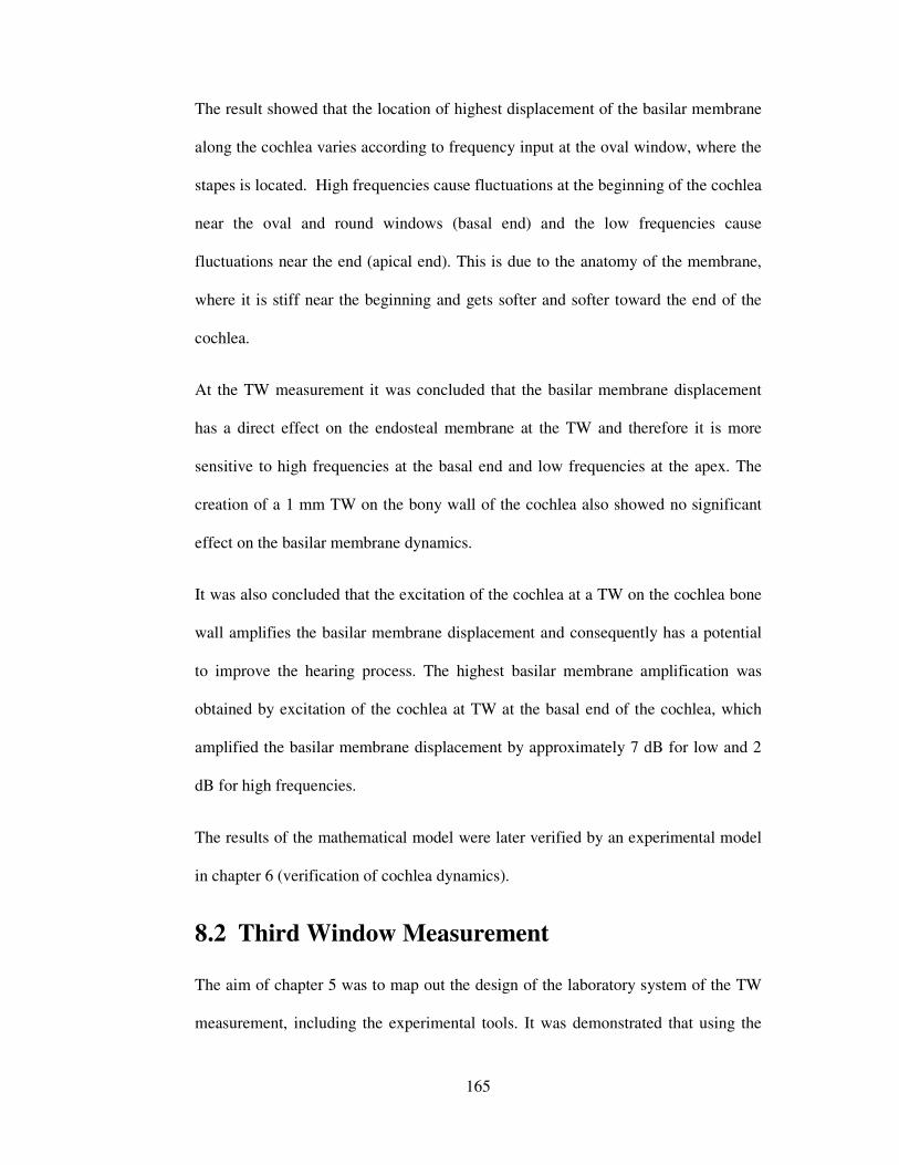
165

The result showed that the location of highest displacement of the basilar membrane

along the cochlea varies according to frequency input at the oval window, where the

stapes is located. High frequencies cause fluctuations at the beginning of the cochlea

near the oval and round windows (basal end) and the low frequencies cause

fluctuations near the end (apical end). This is due to the anatomy of the membrane,

where it is stiff near the beginning and gets softer and softer toward the end of the

cochlea.

At the TW measurement it was concluded that the basilar membrane displacement

has a direct effect on the endosteal membrane at the TW and therefore it is more

sensitive to high frequencies at the basal end and low frequencies at the apex. The

creation of a 1 mm TW on the bony wall of the cochlea also showed no significant

effect on the basilar membrane dynamics.

It was also concluded that the excitation of the cochlea at a TW on the cochlea bone

wall amplifies the basilar membrane displacement and consequently has a potential

to improve the hearing process. The highest basilar membrane amplification was

obtained by excitation of the cochlea at TW at the basal end of the cochlea, which

amplified the basilar membrane displacement by approximately 7 dB for low and 2

dB for high frequencies.

The results of the mathematical model were later verified by an experimental model

in chapter 6 (verification of cochlea dynamics).

8.2 Third Window Measurement

The aim of chapter 5 was to map out the design of the laboratory system of the TW

measurement, including the experimental tools. It was demonstrated that using the

166

robotic micro-drill, it is possible to create a TW at a desired location on the bony

wall of the cochlea and keeping the underlying endosteal membrane intact. This will

give the advantage of restoring the natural dynamics of the cochlea. To carry out the

process a Micro-Scanning Laser Vibrometer (MSV) was used on a porcine hearing

system working through a microscope.

In the last section of the chapter an experiment was used to provide the approach to

distinguish the effect of the vibration of the cochlea as a whole on the vibration

obtained from the endosteal membrane at TW. The result showed a significant

difference between the TW and bone response. Therefore it was concluded that the

TW measurement method is sound and able to observe disturbances within the

closed fluid system of the cochlea and to eliminate normal ambient disturbances that

normal hearing mechanism is sensitive to.

8.3 Experimental Verification of Cochlear Dynamics

The aim of chapter 6 was to investigate the transient disturbances along the path of

cochlea corresponding to the sound vibration, using the TW measurement technique.

In the second part of this chapter the effect TW excitation of the cochlea on the rigid

bone of the cochlea on the disturbances within the cochlea was compared to that of

the stapes excitation at normal hearing.

It was concluded that the findings of the experimental model are in agreement with

the results of the mathematical model in chapter 3. They both suggest the feasibility

of the excitation of the cochlea at a TW in order to amplify cochlear response. This

could specifically assist in cases of hearing difficulties that there is a need for a

direct amplification of cochlea response. The study also suggests that the location of

the excitation can vary according to the frequency band required to be amplified to

167

obtain the optimal results, as the basal end of the cochlea is the high frequency and

the apical end the low frequency region.

8.4 The Influence of Surgical Intervention

The aim of chapter 7 was to contrast the disturbances induced within the cochlea at

different surgical approaches during the different stages at cochlear implantation

process using the TW measurement technique. The results of the study indicate that

the use of robotics will be necessary to minimize the disturbance during the

implantation procedure, which could lead to minimising trauma during the operation.

8.4.1 Cochleostomy formation

In the first part of this study the affect of cochleostomy formation on disturbances

within the cochlea was observed. It was demonstrated that while both drilling speed

and applied force independently effect the movement of the endosteal membrane, the

applied force was the main factor affecting cochlea disturbances. It was concluded

that if the force of drilling can be controlled, and minimized, then the cochlea will

sustain decreased disturbances during the cochleostomy process.

The second part of the study directly compared the disturbances within cochlea by

human and force controlled robotic cochleostomies. The mean membrane velocity

during the robotic drilling is 4% of the velocity when it is drilled manually. Further,

the peak membrane velocity, during the robotic cochleostomy is 1% of the velocity

observed during manual drilling. The robotic micro-drill also kept the underlying

endosteal membrane intact in all the trials.

The studies suggested that control is the key to minimizing disturbance during the

cochleostomy formation. The ability to control the force of drilling and preserve the

168

underlying endosteal membrane will ensure that the traumatic effect of performing a

cochleostomy is reduced to a minimum. The robotic micro-drill is capable of

performance as such at levels not achievable by humans.

8.4.2 Electrode insertion

In this part of the work the effect of insertional speed and the method of insertion

(robotic/manual) on the disturbances of the endosteal membrane were investigated.

It was concluded that increasing electrode array insertion speeds leads to greater

disturbances within the cochlea during the insertion process. It was also concluded

that robotic insertion leads to a lower disturbances of the endosteal membrane than

manual insertion. However, when the speed of the robotic insertion

reached 7000 tp̀ , the disturbances were similar to the manual insertion. The results

suggest that the use of robotic insertion would be less traumatic than manual

insertion due to the constant speed of insertion and elimination of hand tremor and

jerky advancing.

169

Chapter 9. Recommended Future Work

The mathematical model introduced in this work showed it was capable of providing

an understanding of the mechanism of the cochlea, with the development of creation

of a third window (TW) on the bony wall of cochlea and TW excitation. Certain

geometrical and numerical assumptions were taken to obtain the model. Therefore

there is an ongoing work in process to create a mathematical model of the cochlea

with a geometrical parameter close to the empirical cochlea.

So far the primitive frequency map of the exposed endosteal membrane has been

measured along the path of cochlea using the TW measurement technique. The

results suggested the direct relation of the location of frequency input and the region

of highest response. The cochlea was also excited through a TW on different

locations along the bony wall and was concluded that the TW excitation amplifies

the cochlea response in contrast to the stapes excitation. However there is further

works needed to identify the optimal location for middle ear implantation with

respect to maximum efficiency in the transmission of excitation power and to robust

and practical fixation. It is recommended to contrast the disturbances within the

cochlea corresponding to the current middle ear implants (FMT, BAHA) and the TW

excitation at a similar power input.

It was demonstrated that the use of robotic at cochlea implantation procedure will aid

to make a large improvement on human performance in respect to the disturbance

levels within the cochlea. Currently it is assumed that higher disturbance level within

the cochlea means higher trauma to the cochlea, however there is no empirical or

statistical evidence to prove the hypothesis. In the future, there will be a need to

correlate the disturbance levels obtained at a TW by other parameter such as sound

170

pressure level (SPL) to achieve a better understanding of the trauma. There is also a

need to investigate the damage on the biological inner structure of the cochlea. It is

specifically true at the electrode insertion, where the trajectory of the electrode may

cause a risk to damage the fine hair cells of the cochlea.

This work focused on the porcine hearing system as a representative of the human

cochlea. Although there is similarity between the human and porcine cochlea,

nevertheless there is a need to translate the method into successful use in human

hearing system.

171

Appendix

Appendix A. Mathematical model equations and code

In chapter 4 a finite-difference method, the two-dimensional duct was desecrated

into a $% 0 $& grid of points in and � directions. In this model $% , 240

and $& , 8. The derivatives in the Laplace's equation and in the boundary

conditions were replaced by their finite-difference approximations. At each point, an

equation was described for the pressure, in terms of the pressure at the neighbouring

pointsK]�. Then a set of coupled, second-order differential equations was solved in direction

along the path of the cochlea. This was performed by $% discrete points on the

dimension and setting up a large $% 0 $% block-matrix equation; each element of

this block matrix would be a $& 0 $& sub-matrix. This large block matrix is block

tridiagonal. Subsequently, the block-matrix equation would be solved by utilizing a

Gaussian block-elimination technique. An example of solving the equation in form

of block form is as below:

$% , 5 and $& , 4

yzzz{lq /2| 0 0 0/| lI /| 0 00 /| l} /| 00 0 /| l~ 00 0 0 /2| l��

�� yzzz{�q�I�}�~��

�� = yzzz{�0000��

Where

172

l` , ��` /2 0 0/1 4 /1 00 /1 4 /10 0 /2 �`�, �̀ , �K`,qK`,IK`,}K`,~� , �� , yzz

z{/4��IB/4��IB/4��IB/4��IB��

And | is the $% 0 $&identity matrix, and

�` , 4 H 4:��B

The problem is solved using Gaussian block elimination, where the elementary block

operations are used to reduce the system to:

yzzz{| /Wq 0 0 00 | /WI 0 00 0 | /W} 00 0 0 | /W~0 0 0 0 | ��

��

yzzz{�q�I�}�~��

�� = yzzz{�0000��

Where

W] , �2 lhq O , 1 /W]hq H l]�hq 1 N O N $%, � and

�] , �Wq�/2 O , 1 W]�]hq 1 N O N $%, � The final step is the back-substitution:

�] , ��] O , $%,�] H W]�]�q 1 N O N $%, � The coding and computation was done using Matlab program. The first part of the

code is the physical parameter of the membranes. The codes go on to calculate the

173

displacement of the basilar and Endosteal membrane for a certain frequency and

each displacement is plotted against length of the membrane.

rho=.001; %density of water in g/mm3

xmax=25; %length of cochlea in mm

h=1; %height of scalae in mm

d=5; %characteristic length of cochlea in mm

dx = 1/7; %point spacing in mm for finite-diff

x=[0:dx:xmax];

s=10e6*exp(-x/d); %Stiffness of the BM membrane

S=10e6*exp(0); %Stiffness of the EM membrane

beta=2; %Damping

m=0.15*10e-3; %Mass of the BM membrane

M=0.075*10e-3; %Mass of the BM membrane

fo =1000; %frequency of input in Hz

%%

% angular frequency and grid dimensions

wo = 2*pi*fo;

nx = floor(xmax/dx + 1);

ny = floor(h/dx + 1);

%%

% Length of the membranes

position=(0:(nx-1))*dx;

%%

% Stapes Q vector

q1 = -4*rho*(wo^2)*dx;

q = repmat(q1, ny, 1);

174

%%

% BM admittance

y = (1./((s./(i*wo)) + beta + (i*wo*m)));

a=4 + [(4*i*wo*rho*dx).*y ];

% EM admittance

y1 = (1./((S./(i*wo)) + beta + (i*wo*M)));

a1=4 + [(4*i*wo*rho*dx).*y1 ];

%%

% A matrix

A=pascal(ny);

for j=1:ny;

for i=1:ny;

if i-j==0;

A(i,j)=4;

else

A(i,j)=0;

if i-j==-1;

A(i,j)=-1;

else

A(i,j)=0;

if i-j==1;

A(i,j)=-1;

else

A(i,j)=0;

end

175

end

end

end

end

A(1,2)=-2;

A(ny,(ny-1))=-2;

for i=1:length(a);

A(1,1)=a(i);

A(ny,ny)=a(i);

if i == 1;

Am = A;

else

Am = cat(1,Am,A);

end

end

%%

% B matrix

for i=0:(nx-1)

b(((i*ny)+1):((i+1)*ny),(1:ny))=Am(((i*ny)+1):((i+1)*ny)

,(1:ny));

end

176

for i=1:nx

if i==1

B(1:ny,1:ny)=2*inv(b(1:ny,:));

else

B(((i-1)*ny)+1:(i*ny),:)=inv(Am(((i-1)*ny)+1:(i*ny),:)-

B((((i-2)*ny)+1):((i-1)*ny),1:ny));

end

end

B(((nx-1)*ny)+1:(nx*ny),:)=inv((Am(((nx-

1)*ny)+1:(nx*ny),:))-(2*(B(((nx-2)*ny)+1:((nx-

1)*ny),:))));

%%

% C matrix

for i=1:nx

if i==1

C(1:ny,i)=B(1:ny,:)*q*0.5;

else

C(1:ny,i)=B(((i-

1)*ny)+1:(i*ny),:)*C(1:ny,(i-1));

end

177

end

C(1:ny,nx)=2*(B(((nx-1)*ny)+1:(nx*ny),:))*C(1:ny,(nx-

1));

%%

% Pressure along the membranes

for i=fliplr(1:nx)

if i==nx

P(1:ny,nx)=C(1:ny,nx);

else

P(1:ny,i)=C(1:ny,i)+(B(((i-

1)*ny)+1:(i*ny),:)*P(1:ny,(i+1)));

end

end

%%

% Displacement

clear i

X=(y.*P1)/(i*wo);

178

Appendix B. Third window measurement

Below are extra results of the third window (TW) measurement described at chapter

6. For each locations of on the apex, near stapes and near round window (RW) two

sets of graphs are is plotted as a function of frequency.

• On the Apex: A 1 mm TW was 3.77 away from the RW and 4.92 mm from

the stapes.

Figure A-B-1. Measurement on the apex

179

• Near Round window: A 1 mm TW was 1.78 mm away from the RW and

4.45 mm from the stapes.

Figure A-B-2. Measurement point near RW

180

• Near Stapes (RW): A 1 mm TW was 3.10 mm away from the RW and 1.97

mm from the stapes.

Figure A-B-3. Measurement point near stapes

181

References

1. Population Division of the Department of Economic and Social Affairs of the

United Nations Secretariat, World Population Prospects. 2006.

2. Fortnum, H.M., et al., Prevalence of permanent childhood hearing

impairment in the United Kingdom and implications for universal neonatal

hearing screening. Bmj, 2001. 323(7312): p. 536.

3. Cochlear, Cochlea implant: 2009, in Cochlear implant statistics. 2009, The

Ear Foundation: Surrey.

4. Brett, P.P., Implantation time and cost, in Aston University & Queen

Elizabeth Hospital,. 2005: Birmingham, UK.

5. Norman, P.H.L.a.D.A., The ear, showing its three subdivisions -- outer,

middle, and inner. 2007, Thomson Higher Education.

6. Kerr, A.G., Scott-Brown’s Otolaryngology, 6th edn, vols 1–6. 1997, London:

Butterworths.

7. Knutsson, J., Morphology and biochemistry of the tympanic membrane in

relation to retraction pathology.

8. Goode, R.L., et al., New knowledge about the function of the human middle

ear: development of an improved analog model. Otology & Neurotology,

1994. 15(2): p. 145.

9. Manoussaki, D., E.K. Dimitriadis, and R.S. Chadwick, Cochlea’s graded

curvature effect on low frequency waves. SIAM J. Appl. Math Phys Rev Lett,

2000. 96: p. 088701.

10. Nobili, R., F. Mammano, and J. Ashmore, How well do we understand the

cochlea? Trends in Neurosciences, 1998. 21(4): p. 159-167.

11. Doden, E. and R. Halves, On the functional morphology of the human

petrous bone. American Journal of Anatomy, 1984. 169(4): p. 451-462.

12. Holmes, M. and J. Cole, Pseudo-resonance in the cochlea, in Mechanics of

Hearing. 1983: The Netherlands: Martinus Nijhoff.

13. Oghalai, J.S., The cochlear amplifier: augmentation of the traveling wave

within the inner ear. Current opinion in otolaryngology & head and neck

surgery, 2004. 12(5): p. 431.

14. Mäki-Torkko, E.M., M.J. Sorri, and E. Laukli, Objective assessment of

hearing aid use. Scandinavian Audiology, 2001. 30: p. 81-82.

15. Bertoli, S., J. Smurzynski, and R. Probst, Effects of age, age-related hearing

loss, and contralateral cafeteria noise on the discrimination of small

frequency changes: psychoacoustic and electrophysiological measures.

JARO-Journal of the Association for Research in Otolaryngology, 2005.

6(3): p. 207-222.

16. Lee, K.J., Essential otolaryngology: head & neck surgery. 2003: McGraw-

Hill Professional.

17. Mather, G., Foundations of perception. 2006, New York: Taylor & Francis

Inc.

18. Barnes, C.L., B. Stewart, and W.W.H. Gee, Lessons in Elementary Practical

Physics. 1897: Macmillan and Co.

19. Martin, B., The Young Gentleman and Lady's Philosophy. 1781: printed for

W. Owen; and the author.

20. Liberman, A.M. and M. Studdert-Kennedy, Phonetic perception. Perception,

1978: p. 143.

182

21. Von Békésy, G. and E. Wever, Experiments in hearing. 1960: McGraw-Hill

New York.

22. Counter, P., Implantable Hearing Aid. Journal of Engineering in Medicine.

Journal of Engineering in Medicine, 2007(JEIM365).

23. Counter, P., Implantable hearing aids. Proceedings of the Institution of

Mechanical Engineers, Part H: Journal of Engineering in Medicine, 2008.

222(6): p. 837-852.

24. A. Lupsakko, T., H. J. Kautiainen, and R. Sulkava, The non-use of hearing

aids in people aged 75 years and over in the city of Kuopio in Finland.

European Archives of Oto-Rhino-Laryngology, 2005. 262(3): p. 165-169.

25. Todt, I., et al., Magnetic Resonance Imaging Safety of the Floating Mass

Transducer. Otology & Neurotology. 31(9): p. 1435.

26. Schober, M. and S. Almadin, Vibrant MED-EL in Company Brouchure.

2008: Innsbruck (Austria).

27. Gan, R.Z., et al., Mass loading on the ossicles and middle ear function. The

Annals of otology, rhinology & laryngology, 2001. 110(5): p. 478-485.

28. BAHA system. 2011, University of Maryland Medical Center (UMMC):

Baltimore.

29. Béjar-Solar, I., et al., Percutaneous bone-anchored hearing aids at a

pediatric institution. Otolaryngology-Head and Neck Surgery, 2000. 122(6):

p. 887-891.

30. Hickson, L., et al., The Outcomes of Bone Anchored Hearing Aid (BAHA)

Fitting in a Paediatric Cohort. Australian and New Zealand Journal of

Audiology, 2006. 28(2): p. 75-89.

31. Ear with cochlear implant. September 2011, National Institute on Deafness

and Other Communication Disorders: Bethesda.

32. MIMS, Cochlear Implant Clinic. 2011, Malabar Institute of Medical

Sciences Kerala.

33. COCHLEAR IMPLANT SURGERY. 2008, Dallas Ear Institute: Dallas.

34. Kiefer, J., et al., Conservation of low-frequency hearing in cochlear

implantation. Acta oto-laryngologica, 2004. 124(3): p. 272-280.

35. Fishman, K., R. Shannon, and W. Slattery, Speech recognition as a function

of the number of electrodes used in the SPEAK cochlear implant speech

processor. Journal of Speech, Language, and Hearing Research, 1997. 40(5):

p. 1201.

36. Henry, B., C. Turner, and A. Behrens, Spectral peak resolution and speech

recognition in quiet: Normal hearing, hearing impaired, and cochlear

implant listeners. The Journal of the Acoustical Society of America, 2005.

118: p. 1111.

37. Rubinstein, J., et al., Residual speech recognition and cochlear implant

performance: effects of implantation criteria. Otology & Neurotology, 1999.

20(4): p. 445.

38. vonIlberg, C., et al., Electric-acoustic stimulation of the auditory system.

ORL, 2000. 61(6): p. 334-340.

39. Zou, J., et al., Sensorineural hearing loss after vibration: an animal model

for evaluating prevention and treatment of inner ear hearing loss. Acta oto-

laryngologica, 2001. 121(2): p. 143-148.

40. Tos, M., Surgical solutions for conductive hearing loss. Vol. 4. 2000:

Thieme.

183

41. Briggs, R., et al., Cochleostomy site: implications for electrode placement

and hearing preservation. Acta oto-laryngologica, 2005. 125(8): p. 870-876.

42. Roland, P., W. Gstöttner, and O. Adunka, Method for hearing preservation in

cochlear implant surgery. Operative Techniques in Otolaryngology-Head and

Neck Surgery, 2005. 16(2): p. 93-100.

43. Du Verney, J., Traité de l'organe de l'ouïe: contenant la structure, les usages

et les maladies de toutes les parties de l'oreille: Paris: Chez Estienne

Michallet, 1683.

44. Gelfand, S.A. and H. Levitt, Hearing: An introduction to psychological and

physiological acoustics. 1998: Marcel Dekker.

45. Neely, S., Finite difference solution of a two-dimensional mathematical

model of the cochlea. J. Acoust. Soc. Am, 1981. 69(5): p. 1386–1393.

46. Andor, D., et al., Wave propagation by critical oscillators. 2006.

47. An uncoiled cochlea, to the right of the oval and round windows, in NIH

Curriculum Supplement Series 2007, National Institutes of Health (US);

Biological Sciences Curriculum Study: Bethesda MD.

48. Duke, T. and F. Jülicher, Active traveling wave in the cochlea. Physical

review letters, 2003. 90(15): p. 158101.

49. Neely, S. and D. Kim, An active cochlear model showing sharp tuning and

high sensitivity. Hearing research, 1983. 9(2): p. 123-130.

50. Loh, C., Multiple scale analysis of the spirally coiled cochlea. The Journal of

the Acoustical Society of America, 1983. 74: p. 95.

51. Steele, C. and L. Taber, Comparison of WKB calculations and experimental

results for three dimensional cochlear models. The Journal of the Acoustical

Society of America, 1979. 65: p. 1007.

52. Manley, G., Cochlear mechanisms from a phylogenetic viewpoint.

Proceedings of the National Academy of Sciences of the United States of

America, 2000. 97(22): p. 11736.

53. Manoussaki, D., et al., The influence of cochlear shape on low-frequency

hearing. Proceedings of the National Academy of Sciences, 2008. 105(16): p.

6162.

54. Marquardt, T., et al., Low-frequency characteristics of human and guinea pig

cochleae. The Journal of the Acoustical Society of America, 2007. 121: p.

3628.

55. Givelberg, E. and J. Bunn, A comprehensive three-dimensional model of the

cochlea* 1. Journal of Computational Physics, 2003. 191(2): p. 377-391.

56. Dallos, P., Low frequency auditory characteristics: species dependence. The

Journal of the Acoustical Society of America, 1970. 48: p. 489.

57. Karavitaki, K. and D. Mountain, In: Biophysics of the Cochlea: From

Molecules to Models. Gummer AW, editor. 2003, Singapore: World

Scientific.

58. Gan, R., B. Reeves, and X. Wang, Modeling of sound transmission from ear

canal to cochlea. Annals of biomedical engineering, 2007. 35(12): p. 2180-

2195.

59. Wysocki, J., Dimensions of the vestibular and tympanic scalae of the cochlea

in selected mammals. Hearing research, 2001. 161(1-2): p. 1-9.

60. Tapering of the uncoiled Cochlea, in Thomson Higher Education. 2007.

61. Koshigoe, S., W. Kwok, and A. Tubis, Effects of perilymph viscosity on low

frequency intracochlear pressures and the cochlear input impedance of the

cat. The Journal of the Acoustical Society of America, 1983. 74: p. 486.

184

62. Lüling, H., J. Franosch, and J. van Hemmen, A two-dimensional cochlear

fluid model based on conformal mapping. The Journal of the Acoustical

Society of America. 128(6): p. 3577.

63. Siebert, W., Ranke Revisited—a Simple Short Wave Cochlear Model. The


64. Allen, J., Two dimensional cochlear fluid model: New results. The Journal of


65. Pozrikidis, C., Boundary-integral modeling of cochlear hydrodynamics.

Journal of Fluids and Structures, 2008. 24(3): p. 336-365.

66. Hamilton, T., et al. Analogue VLSI implementations of two dimensional,

nonlinear, active cochlea models. 2009: IEEE.

67. Ku, E.M., Modelling the Human Cochlea, in Faculty of Engineering, Science

and Mathematics. 2008, University of Southampton: Southampton.

68. Watts, L., cochlea mechanics: Analysis and Analog VLSI, in Institute of

Technology. 1993: Pasadena, California.

69. Steele, C. and L. Taber, Three dimensional model calculations for guinea pig

cochlea. The Journal of the Acoustical Society of America, 1981. 69: p.

1107.

70. de Boer, E., A. Nuttall, and C. Shera, Wave propagation patterns in a"

classical" three-dimensional model of the cochlea. The Journal of the

Acoustical Society of America, 2007. 121(1): p. 352.

71. Takagi, A. and I. Sando, Computer-aided three-dimensional reconstruction:

a method of measuring temporal bone structures including the length of the

cochlea. The Annals of otology, rhinology, and laryngology, 1989. 98(7 Pt

1): p. 515.

72. Steele, C., Behavior of the basilar membrane with pure tone excitation. The


73. Mistrík, P., et al., Three-dimensional current flow in a large-scale model of

the cochlea and the mechanism of amplification of sound. Journal of The

Royal Society Interface, 2009. 6(32): p. 279.

74. Elliott, S., B. Lineton, and G. Ni, Fluid coupling between the elements in a

discrete model of cochlear mechanics.

75. Farlow, S., Partial differential equations for scientists and engineers. 1993:

Dover Pubns.

76. Obrist, D., Transient inviscid flow in a passive linear model of the cochlea.

PAMM, 2009. 9(1): p. 477-478.

77. Prikkel, J., Modelling cochlear mechanics, in Faculty of mathematics and

natural sciences. 2009, University of Groningen. p. 2395.

78. Eze, N. and E. Olson, Basilar Membrane Velocity in a Cochlea with a

Modified Organ of Corti. Biophysical Journal, 2011. 100(4): p. 858-867.

79. Kolston, P.J., The importance of phase data and model dimensionality to

cochlear mechanics. 2000, Hearing Research.

80. Brett, P., et al. A surgical robot for cochleostomy. 2007: IEEE.

81. Coulson, C., et al., An autonomous surgical robot for drilling a

cochleostomy: preliminary porcine trial. Clinical Otolaryngology, 2008.

33(4): p. 343-347.

82. Robles, L. and M.A. Ruggero, Mechanics of the mammalian cochlea.

Physiological reviews, 2001. 81(3): p. 1305-1352.

83. Johnstone, B. and A. Boyle, Basilar membrane vibration examined with the

Mossbauer technique. Science, 1967. 158: p. 389-390.

185

84. Rhode, W.S., Observations of the vibration of the basilar membrane in

squirrel monkeys using the Mössbauer technique. The Journal of the

Acoustical Society of America, 1971. 49: p. 1218.

85. Rhode, W. and L. Robles, Evidence from Mössbauer experiments for

nonlinear vibration in the cochlea. The Journal of the Acoustical Society of

America, 1974. 55: p. 588.

86. Rhode, W., An investigation of postmortem cochlear mechanics using the

Mössbauer effect. Basic mechanisms in hearing, 1973: p. 49-67.

87. Ruggero, M., Responses to sound of the basilar membrane of the mammalian

cochlea. Current Opinion in Neurobiology, 1992. 2(4): p. 449-456.

88. Ruggero, M., et al., Basilar Membrane Responses to Two-Tone and

Broadband Stimuli [and Discussion]. Philosophical Transactions: Biological

Sciences, 1992. 336(1278): p. 307-315.

89. Sellick, P., R. Patuzzi, and B. Johnstone, Measurement of basilar membrane

motion in the guinea pig using the Mössbauer technique. The Journal of the


90. Sellick, P., R. Patuzzi, and B. Johnstone, Comparison between the tuning

properties of inner hair cells and basilar membrane motion. Hearing

research, 1983. 10(1): p. 93-100.

91. Sellick, P., G. Yates, and R. Patuzzi, The influence of Mossbauer source size

and position on phase and amplitude measurements of the guinea pig basilar

membrane. Hearing research, 1983. 10(1): p. 101-108.

92. Choudhury, N., et al., Low coherence interferometry of the cochlear

partition. Hearing research, 2006. 220(1-2): p. 1-9.

93. Wilson, J. and J. Johnstone, Basilar membrane and middle- ear vibration in

guinea pig measured by capacitive probe. The Journal of the Acoustical

Society of America, 1975. 57: p. 705.

94. LePage, E., Functional role of the olivo-cochlear bundle: a motor unit

control system in the mammalian cochlea. Hearing research, 1989. 38(3): p.

177-198.

95. Xue, S., D. Mountain, and A. Hubbard, Electrically evoked basilar

membrane motion. The Journal of the Acoustical Society of America, 1995.

97: p. 3030.

96. Cook, R. and C. Hamm, Fiber optic lever displacement transducer. Applied

Optics, 1979. 18(19): p. 3230-3241.

97. Zhang, K., et al., Optoacoustic induced vibrations within the inner ear.

Optics Express, 2009. 17(25): p. 23037-23043.

98. Dai, C. and R. Gan, Change in Cochlear Response in an Animal Model of

Otitis Media with Effusion. Audiology and Neurotology, 2009. 15(3): p. 155-

167.

99. Stenfelt, S., et al., Basilar membrane and osseous spiral lamina motion in

human cadavers with air and bone conduction stimuli. Hearing research,

2003. 181(1-2): p. 131-143.

100. Overstreet, E.H., A.N. Temchin, and M.A. Ruggero, Basilar membrane

vibrations near the round window of the gerbil cochlea. JARO-Journal of the

Association for Research in Otolaryngology, 2002. 3(3): p. 351-361.

101. Ruggero, M. and N. Rich, Application of a commercially-manufactured

Doppler-shift laser velocimeter to the measurement of basilar-membrane

vibration. Hearing research, 1991. 51(2): p. 215-230.

186

102. Brundin, L., et al., Frequency-specific position shift in the guinea pig organ

of Corti. Neuroscience letters, 1991. 128(1): p. 77-80.

103. Willemin, J., R. Dändliker, and S. Khanna, Heterodyne interferometer for

submicroscopic vibration measurements in the inner ear. The Journal of the


104. Nuttall, A., D. Dolan, and G. Avinash, Laser doppler velocimetry of basilar

membrane vibration. Hearing research, 1991. 51(2): p. 203-213.

105. Cooper, N., An improved heterodyne laser interferometer for use in studies of

cochlear mechanics. Journal of neuroscience methods, 1999. 88(1): p. 93-

102.

106. Cooper, N. and W. Rhode, Basilar membrane mechanics in the hook region

of cat and guinea-pig cochleae: sharp tuning and nonlinearity in the absence

of baseline position shifts. Hearing research, 1992. 63(1-2): p. 163-190.

107. Khanna, S.M., J.F. Willemin, and M. Ulfendahl, Measurement of optical

reflectivity in cells of the inner ear. Acta oto-laryngologica. Supplementum,

1989(467): p. 69-75.

108. Cooper, N., Vibration of beads placed on the basilar membrane in the basal

turn of the cochlea. The Journal of the Acoustical Society of America, 1999.

106: p. L59.

109. Fletcher, H., The mechanism of hearing as revealed through experiment on

the masking effect of thermal noise. Proceedings of the National Academy of

Sciences of the United States of America, 1938. 24(7): p. 265.

110. Su, W., et al., Anatomical measurements of the cochlear aqueduct, round

window membrane, round window niche, and facial recess. The

Laryngoscope, 1982. 92(5): p. 483-486.

111. Kringlebotn, M., The equality of volume displacements in the inner ear

windows. The Journal of the Acoustical Society of America, 1995. 98: p. 192.

112. Stenfelt, S., N. Hato, and R.L. Goode, Round window membrane motion with

air conduction and bone conduction stimulation. Hearing research, 2004.

198(1-2): p. 10-24.

113. Aibara, R., et al., Human middle-ear sound transfer function and cochlear

input impedance. Hearing research, 2001. 152(1-2): p. 100-109.

114. Stenfelt, S., N. Hato, and R.L. Goode, Fluid volume displacement at the oval

and round windows with air and bone conduction stimulation. The Journal of


115. Huber, A., et al., The Influence of a Cochlear Implant Electrode on the

Mechanical Function of the Inner Ear. Otology & Neurotology. 31(3): p.

512.

116. Pau, H., et al., Noise exposure of the inner ear during drilling a cochleostomy

for cochlear implantation. The Laryngoscope, 2007. 117(3): p. 535-540.

117. MED-EL, The Versatile FMT, in MED-EL Website. 2010: Innsbruck,

Austria.

118. Needham, A., et al., The effects of mass loading the ossicles with a floating

mass transducer on middle ear transfer function. Otology & Neurotology,

2005. 26(2): p. 218.

119. Wilkes, E., BAHA energy flow to the cochlea in Cochlear Ltd. 2007 Hearing

Therapy Australia

120. Brett, P., et al. A surgical robot for cochleostomy. in Conference of the IEEE

EMBS. 2007. Cité Internationale, Lyon, France.

187

121. Nakajima, H., et al., Evaluation of round window stimulation using the

floating mass transducer by intracochlear sound pressure measurements in

human temporal bones. Otology & neurotology: official publication of the

American Otological Society, American Neurotology Society [and] European

Academy of Otology and Neurotology. 31(3): p. 506.

122. Roberson, J.B., Alternative placement of the floating mass transducer in

implanting the MED-EL Vibrant Soundbridge. Operative Techniques in

Otolaryngology-Head and Neck Surgery. 21(3): p. 194-196.

123. Colletti, V., et al., Treatment of mixed hearing losses via implantation of a

vibratory transducer on the round window. International journal of

audiology, 2006. 45(10): p. 600-608.

124. Kiefer, J., W. Arnold, and R. Staudenmaier, Round Window stimulation with

an implantable hearing aid (Soundbridge®) combined with autogenous

reconstruction of the auricle–a new approach. Cochlear Mechanics and

Otoacoustic Emissions, 68: 378-385. ORL, 2006.

125. Shimizu, Y., S. Puria, and R.L. Goode, The Floating Mass Transducer on the

Round Window Versus Attachment to an Ossicular Replacement Prosthesis.

Otology & Neurotology. 32(1): p. 98.

126. Witte, R.J., et al., Pediatric and Adult Cochlear Implantation1.

Radiographics, 2003. 23(5): p. 1185.

127. Roland, P.S., W. Gstöttner, and O. Adunka, Method for hearing preservation

in cochlear implant surgery. Operative Techniques in Otolaryngology-Head

and Neck Surgery, 2005. 16(2): p. 93-100.

128. Gantz, B. and C. Turner, Combining acoustic and electrical speech

processing: Iowa/Nucleus hybrid implant. Acta oto-laryngologica, 2004.

124(4): p. 344-347.

129. James, C., et al., Preservation of residual hearing with cochlear

implantation: how and why. Acta oto-laryngologica, 2005. 125(5): p. 481-

491.

130. Kiefer, J., et al., Conservation of low-frequency hearing in cochlear

implantation. Acta oto-laryngologica, 2004. 124(3): p. 272-280.

131. Gstoettner, W., et al., Hearing preservation in cochlear implantation for

electric acoustic stimulation. Acta oto-laryngologica, 2004. 124(4): p. 348-

352.

132. Coulson, C., et al., ENT challenges at the small scale. The International

Journal of Medical Robotics and Computer Assisted Surgery, 2007. 3(2): p.

91-96.

133. Lehnhardt, E., Intracochlear placement of cochlear implant electrodes in soft

surgery technique. Hno, 1993. 41(7): p. 356.

134. Brett, P., et al. An Autonomous Surgical Robot Applied in Practice. 2008:

Springer.

135. Electrode curls into the inner ear (cochlea), in Cochlear company website.

2008, Cochlear company: Sydney.

136. Rebscher, S.J., et al., Considerations for the design of future cochlear

implant electrode arrays: Electrode array stiffness, size and depth of

insertion. Journal of rehabilitation research and development, 2008. 45(5): p.

731.

137. Briggs, R.J.S., et al., Cochleostomy site: implications for electrode placement

and hearing preservation. Acta oto-laryngologica, 2005. 125(8): p. 870-876.

188

138. Schurzig, D., et al. A Force Sensing Automated Insertion Tool for Cochlear

Electrode Implantation.

139. Wise, K., et al., High-density cochlear implants with position sensing and

control. Hearing research, 2008. 242(1-2): p. 22-30.

140. Huber, A.M., et al., The Influence of a Cochlear Implant Electrode on the

Mechanical Function of the Inner Ear. Otology & Neurotology, 2010. 31(3):

p. 512.

141. Donnelly, N., A. Bibas, and D. Jiang, Effect of cochlear implant electrode

insertion on middle-ear function as measured by intra-operative laser

Doppler vibrometry. The Journal of Laryngology & Otology, 2009. 123: p.

723-729.

142. Neely, S., Mathematical modeling of cochlear mechanics. J. Acoust. Soc.

Amer, 1985. 78(1): p. 345–352.

143. Watts, L., Cochlear mechanics: Analysis and analog VLSI, in California

Institute of Technology. 1992, California Institute of Technology: California.

144. De Boer, E., Mechanics of the cochlea: modeling efforts. Springer Handbook

of Auditory Research, 1996. 8: p. 258-317.

145. Lighthill, J., Energy flow in the cochlea. Journal of fluid mechanics, 2006.

106: p. 149-213.

146. Viergever, M. and T. Delft Mechanics of the inner ear a mathematical

approach. 1980: Belgium.

147. Lyon, R. and C. Mead, Cochlear hydrodynamics demystified. California

Institute of Technology, 1988.

148. Van den Nieuwenhof, B. and J. Coyette, Treatment of frequency-dependent

admittance boundary conditions in transient acoustic finite/infinite-element

models. The Journal of the Acoustical Society of America, 2001. 110: p.

1743.

149. Sondhi, M., Method for computing motion in a two dimensional cochlear

model. The Journal of the Acoustical Society of America, 1978. 63: p. 1468.

150. Kagawa, Y., et al., Finite element cochlear models and their steady state

response. Journal of Sound and Vibration, 1987. 119(2): p. 291-315.

151. Press, W., et al., Numerical recipes. 2007: Cambridge university press

Cambridge.

152. Yost, W.A. and D.W. Nielsen, Fundamentals of Hearing. New York: Holt,

Rinehart and Winston. 1977, PART.

153. Zweig, G. Basilar membrane motion. 1976: Cold Spring Harbor Laboratory

Press.

154. Coulson, C., et al., An autonomous surgical robot for drilling a

cochleostomy: preliminary porcine trial. Clin Otolaryngol, 2008. 33(4): p.

343-347.

155. Taylor, R., et al., A sensory-guided surgical micro-drill. Proceedings of the

Institution of Mechanical Engineers, Part C: Journal of Mechanical

Engineering Science. 224(7): p. 1531-1537.

156. Pracy, J.P., et al., The comparative anatomy of the pig middle ear cavity: a

model for middle ear inflammation in the human? Journal of Anatomy, 1998.

192(03): p. 359-368.

157. MSV-400 Microscope Scanning Vibrometer-Features. MSV-400 Microscope

Scanning Vibrometer 2008.

158. Zhu, Z. and W. Li, Integration of laser vibrometry with infrared video for

multimedia surveillance display. AFRL Final Performance Report, ccny.

189

cuny. edu/~ zhu/LDV/FinalReportsHTML/CCNYLDV-Tech-Report-html.

htm, 2005.

159. Yarlagadda, P.K.D.V. and S. Narayanan, GCMM 2004: 1st International

Conference on Manufacturing and Management. 2005: Alpha Science Intl

Ltd.

160. Huber, A., et al., Intraoperative assessment of stapes movement. ANNALS

OF OTOLOGY RHINOLOGY AND LARYNGOLOGY, 2001. 110(1): p.

31-35.

161. Piotrowska, A., et al., Analysis of Factors Affecting Hearing Preservation

after Cochlear Implantation. Cochlear Implants International. 11(Supplement

1): p. 114-116.

162. Pau, H., et al., Noise exposure of the inner ear during drilling a cochleostomy

for cochlear implantation. Laryngoscope, 2007. 117(3): p. 535-540.

163. Gantz, B., et al., Preservation of hearing in cochlear implant surgery:

advantages of combined electrical and acoustical speech processing.

Laryngoscope, 2005. 115(5): p. 796-802.

164. Coulson, C., P. Slack, and X. MA, The effect of supporting a surgeon's wrist

on their hand tremor. Microsurgery.

165. Lehnhardt, E. and R. Laszig, Specific surgical aspects of cochlear implant

soft surgery. Advances in Cochlear Implants. Vienna, Manz, 1994: p. 228-

229.

166. Gantz, B.J. and C.W. Turner, Combining acoustic and electrical hearing.

The Laryngoscope, 2003. 113(10): p. 1726-1730.

167. Gstoettner, W., et al., Hearing preservation in cochlear implantation for

electric acoustic stimulation. Acta oto-laryngologica, 2004. 124(4): p. 348-

352.

168. Donnelly, N., et al., Effect of cochlear implant electrode insertion on middle-

ear function as measured by intra-operative laser Doppler vibrometry. The

Journal of Laryngology & Otology, 2009. 123(07): p. 723-729.

169. Schurzig, D., et al. A force sensing automated insertion tool for cochlear

electrode implantation. 2010: IEEE.

170. Adunka, O., et al., Cochlear implantation via the round window membrane

minimizes trauma to cochlear structures: a histologically controlled insertion

study. Acta oto-laryngologica, 2004. 124(7): p. 807-812.

an investigation of cochlear dynamics in surgical …

Documents