An investigation into the use of Cross

Correlation Velocimetry

A Masters Thesis Submitted to the Faculty of the

Worcester Polytechnic Institute

in partial fulfilment of the requirements for the

Degree of Master of Science in

Fire Protection Engineering.

December 2009

____________________________

Scott R. Rockwell

Approved:

__________________________________

Professor Ali S. Rangwala, Advisor

__________________________________

Professor Andy Klein, Co-Advisor

__________________________________

Professor Kathy A. Notarianni,

Co-Advisor & Head of Department

2

Index:

Index ................................................................................................................................. 2

Introduction ...................................................................................................................... 3

Chapter 1 – Frequency and Spatial Dependence of Cross Correlation Velocimetry ....... 6

Chapter 2 – An Examination of Cross Correlation Velocimetry’s Ability to Predict Characteristic

Turbulent Length Scales in Fire Induced Flow................................................................. 16

Chapter 3 – Cross Correlation Velocimetry in Turbulent Fire-Induced Flows................ 27

Chapter 4 - Future work ................................................................................................... 50

Appendix 1 – MATLAB post processing script ............................................................... 54

Appendix 2 – WPI Annual Showcase of Graduate Research 2008 poster ....................... 63

Appendix 3 – International Association of Fire Safety Science (IAFSS) 2008 poster .... 64

3

Introduction:

The objective of this thesis was to use current technology to examine Cross Correlation

Velocimetry (CCV) as a cheaper velocity sensor than those available to the research community

currently. A sensor was developed which can measure temperature, velocity, and the integral

turbulent length scale of a flow simultaneously. While CCV has been used for many years this

work analysed higher sampling rates, sampling times, than prior work reported in literature. In

addition, this study also analyses the application of CCV to low velocity flows (~0.1 m/s).

The thesis is laid out in 3 chapters plus a future work section and appendices. Each of the

three chapters is a paper which was either presented at a conference or is in the process of being

submitted for publication. Chapter 1 is a paper titled Frequency and Spatial Dependence of

Cross Correlation Velocimetry and was presented at the Central States Section of the

Combustion Institute, University of Alabama, April 20-22, 2008. This paper discusses the need

for cross correlation velocimetry, the history of the use of this technique in fire and other areas of

research, and presents preliminary results. These preliminary results used an axi-symmetric jet

and a hot wire anemometer as a reference measurement. Both the frequency dependence and the

dependence of CCV on the separation of the thermocouples is presented. The purpose of this

study was not to prove that CCV works to measure velocity because this had been shown in

previous literature, the purpose was to prove that the CCV technique was viable in the

experimental setup built for this study and to begin to look at spatial and frequency dependences

of the technique. A velocity of 1.1 m/s was used as the velocity to show the validity of the

technique because it was in the middle of the range of velocities used in previous literature, a

wider range of velocities is presented in later chapters of this work. Sampling frequencies up to

3 kHz were used in this work because it is representative of what had been found in literature so

far, larger sampling frequencies are presented in later chapters of this work. This paper explains

that there are multiple factors which effect the CCV technique; sampling frequency, TC response

time, TC separation distance, turbulent eddy size, soot accumulation, equality of TC time

constants, and sampling period. Other than the sampling frequency and separation distance all

the other factors were held constant at a value believed to be reasonable based on previous

literature. It was found that at the velocity of 1.1 m/s the optimum separation distance was

15mm and the sampling frequency above 500 Hz had little effect. While these are not

universally applicable results the purpose of this portion of the experiment was completed

showing that the CCV technique was viable for the experimental setup which was built and

allowed the expansion of the studies. The hot wire anemometer was susceptible to temperature

changes, therefore in later experiments an Laser Doppler Anemometer (LDA) was used as the

reference measurement. Since the LDA is a non-invasive technique both the CCV and LDA

measurements could be taken simultaneously as discussed in chapter 2 and 3.

Chapter 2 is a paper titled An Examination of Cross Correlation Velocimetry’s Ability to

Predict Characteristic Turbulent Length Scales in Fire Induced Flows and was presented at the

Eastern States Section of the Combustion Institute, University of Maryland, College Park,

October 18-21, 2009. This paper presents a use for the CCV technique which to the author’s

knowledge has not been published in literature before. This paper discusses the use of a CCV

sensor to measure turbulent length scales in both a heated axi-symmetric jet and above a variable

diameter natural gas burner. A new axi-symmetric jet was built for use in these studies and an

4

LDA was used as the reference velocity measurement. Using a triple CCV probe, which is a

CCV probe which uses three thermocouples at two different separation distances, it was found

that the CCV technique could predict the characteristic length scale, which was taken to be an

85% decay in either the centreline velocity or temperature, within 6.5% of the width measured

by a the decay in the LDA and within 13.5% of a correlation published by Kanury (An

Introduction to Combustion Phenomena, Gordon and Breach Pub, 1975). The triple probe was

also tested over a natural gas plume and the CCV technique could measure the characteristic

length within 25% of the width measured by a horizontal thermocouple tree and the width

predicted by Heskestad’s correlation. The average difference between the CCV technique and

thermocouple measurements was 8.4% and reasons for this variation are discussed in this

chapter. It was shown that CCV could be used for multiple applications including estimation of

the mass flux in a plume as well as the ceiling jet thickness. The methodology, possible uses,

and assumptions involved with this technique are discussed in this chapter.

Chapter 3 is a paper titled Exploring Cross Correlation Velocimetry in Turbulent Fire-

Induced Flows, and is planned to be submitted to Fire Technology. This paper presents a

thorough examination of the work which was done using the CCV and covers the sampling time,

sampling rate, and measured velocities when using a CCV. In addition, the work discusses the

angular dependence of the one dimensional CCV with respect to the bulk flow and how this

dependence can be corrected. . Experiments were once again, conducted over an axi-symmetric

jet and a variable diameter natural gas burner discussed in chapter 2.

The E type 0.003” thermocouples were used because they represent the smallest

thermocouples commercially available and are similar to the thermocouples used previously used

in literature. As discussed in this chapter CCV is affected by nine main factors (two more factors

were added from chapters 1): thermocouple separation distance, sampling period, sampling

frequency, the alignment of the CCV probe with the bulk flow, thermocouple response time, soot

accumulation, equality of thermocouple response time, turbulent eddy size, and the magnitude of

the thermal gradients in the flow. This study examines the first four of these factors; these are

the fundamental factors required to use the CCV technique in the field. The last 5 factors are set

the bounds of where the thermocouples can be used. The effects of response time, and equality

of response time are shown in previous literature. Soot effects were not characterized due to

time and laboratory availability limitation but are discussed in the future work section of this

paper. Turbulent eddy size varies depending on the flow condition along with the magnitude of

the thermal gradients in the flow and it is discussed that for CCV to work the separation distance

of the thermocouples needs to be smaller than the maximum turbulent eddy size and that the

CCV technique is done in temperature conditions ranging from 2C above ambient conditions to

100C above ambient conditions though the absolute maximum and minimum conditions were

not found.

It was shown that the CCV could measure velocity within 5% of an LDA measurement

when using a linear correction factor, the separation distance did not effect the CCV

measurement at a sampling rate of 10 kHz and velocity of 2m/s or below. Lower sampling rates

effected the non dimensional (ND) cross correlation coefficient and a sampling rate of 2KHz was

found to be optimal for the axi-symmetric jet scenario. The sampling time affects both the

correlation coefficient and the standard deviation of the velocity measurement. For a robust

CCV measurement the standard deviation of the velocity measurement should be low (the

5

standard deviation of the LDA was used as the baseline for comparison) and the ND cross

correlation coefficient should be high (close to 1), it was found that between 4 and 8 seconds of

data was needed depending on the velocity of the data. The effect of angular offset with respect

to the probe was studied from between 0-40, it was found that a correction could be made

which reduced the error induced by the offset from over 25% to less than 10% if the offset angle

is known.

It was determined that rather than predicting the characteristic turbulent length scale as

discussed in chapter 2 the CCV technique measured the integral length scale which is known to

be slightly small but on the same order of magnitude as discussed in this chapter. The integral

length scale is more useful than the characteristic length scale in terms of working with

computational fluid dynamic models.

The future work section discusses the need to test the last three factors effecting the probe

including the effects of soot deposition, turbulent size effects, and the effects of temperature

gradients, the last two of which were only touched on briefly in this work. Also testing the probe

in full scale fire tests and creating hardware to provide real time measurements should be

accomplished. The prospect of obtaining multi-dimensional velocity data is also discussed. An

idea for creating a robust 1D probe which can be used with minimal effect of flow angle is

presented. Also an optimised data analysis technique is shown along with a theoretical method

for using the CCV technique in isothermal flows.

Three appendices are included at the end of this work, the MATLAB script used to

analyse the thermocouple data, and two posters presented of this work. Appendix 1 includes the

MATLAB script used to analyse the thermocouple data, this script is self inclusive using a

custom cross correlation script developed to minimise the edge effects of a standard correlation

technique. The script automatically imports a series of tests and outputs the results, the script is

capable of either series sampling or overlapping sampling as discussed in the future work

section, and performs an autocorrelation of one of the signals so that a check can be made to

make sure that Taylor’s hypothesis is holding in the flow being studied.

Appendix 2 includes a poster presented at WPI’s Annual Showcase of Graduate Research

in 2008, it shows the experimental setup and results discussed in chapter 1 in a visual form rather

than a text form. Preliminary results of the effects of thermocouple separation distance and

sampling frequency using the small axi-symmetric jet with the hot wire anemometer as the

reference measurement are presented.

Appendix 3 includes a poster presented at the 2008 International Association of Fire

Safety Science Conference hosted by the University of Karlsruhe in Karlsruhe, Germany;

September 21-26 2008. This poster shows the large axi-symmetric jet with the LDA and CCV.

The poster presents the work of the initial study into the effects of the separation distance and the

effects of sampling frequency using the large ax-symmetric jet. The poster discusses the

attempts to create the hardware for real time cross correlation using a Digital Signal Processor

(DSP) chip. An undergraduate ECE researcher who was hired to help with the project performed

this work. While the real time algorithms were developed, due to memory limitations with the

chip the ability to do real time CCV calculations was not completed in the time frame allotted by

the funding.

6

Chapter 1:

Frequency and Spatial Dependence of Cross Correlation

Velocimetry (Presented at the Central States Section of the Combustion Conference 2008)

Scott R. Rockwell1*, Ali S. Rangwala

2

Department of Fire Protection Engineering

Worcester Polytechnic Institute

Worcester, MA

Abstract This study analyses the frequency and spatial dependence of Cross Correlation Velocimetry (CCV) towards

the measurement of fire induced flows. CCV uses temperature-time records from a pair of thermocouples, one

downstream of the other, cross-correlated to determine the flow's velocity and is based in principle on the “frozen

eddy” concept in turbulent flows. In between 1975 and 1980 Cox et al. (Cox) performed a series of experiments that

showed that spatial and temporally resolved velocity measurements could be achieved by means of CCV. These

types of velocity measurements are crucial in understanding ceiling jets, the role of sprinkler activation, and also in

micro-gravity fire induced flows that conventional techniques cannot measure. However, the high cost associated

with expensive analogue correlators available those days caused the CCV technique to gradually phase out after the

advent of the bidirectional probe which was significantly cheaper and more robust in design. There have been vast

improvements in data acquisition techniques, digital signal conditioning, filtration of random noise, as well post

processing statistical packages which allow better and faster cross correlation of two random signals. This study is a

first step towards applying these technological advantages to this outdated technique.

The CCV probe’s accuracy is most sensitive to the thermocouple wire diameter, separation distance, and

speed of data acquisition (sampling frequency). This study presents a parameter sensitivity analysis that includes the

measurement of axial components of velocity in a heated turbulent jet with a velocity of 1.1 m/s with the sampling

frequency, and probe separation distance adjusted independently (thermocouple wire diameter is kept constant).

Nomenclature:

A = Surface Area (m2)

Cp = Specific Heat (J/(kg °C))

d = Distance between Thermocouples (mm)

f = Sampling Frequency (Hz)

h = Average Convective Heat Transfer Coefficient (kW/m2)

Rxy = Cross correlation function of x(t) and y(t) (-)

t = Time (s)

T = Averaging Time (s)

Tmax = Maximum temperature (°C)

Tave = Average Temperature (°C)

v = Velocity (m/s)

V = Volume (m3)

x(t) = Temperature profile (°C)

y(t) = Temperature profile (°C)

ρ = Density (kg/m3)

θ = Non Dimensional Time (ND)

τ = Time lag (s)

τs = Spacing Lag (-)

τR = Response Time (s)

1 Graduate Research Assistant (Goddard Fellow), Department of Fire Protection Engineering, WPI

2 Professor, Department of Fire Protection Engineering, WPI

* Corresponding Author: srockwel@wpi.edu

Proceedings of the 2008 Technical Meeting of the Central States Section of The Combustion Institute

7

Introduction:

Accurate measurement of temperature and velocity fields created by fire plumes

is vital in quantifying the thermal impact of a fire. Both play a major role in the prediction of

smoke detector and sprinkler activation, design of smoke venting systems, and estimation of

egress times. In addition, accurate knowledge of temperature and velocity of fire induced flows

is crucial in the determination of structural integrity in a fire environment. While temperatures

can be measured accurately using array’s of thermocouples, the field of fire science lacks an

economical method of measuring velocity fields (Grosshandler).Table 1 shows velocity

measurement methods currently in use. Bi-directional probes have been used successfully to

determine the velocities in doorways and other areas where the general direction of the flow is

known. The disadvantage of this type of system is that the probes are large (causing flow

obstruction), and suffer from calibration problems. In addition, the bidirectional probe becomes

inaccurate at flows lower than 0.5 m/s (Sette). The pitot tube is not heavily used in the fire field

due to the small size of the pressure tap holes which can become clogged with soot. The hot

wire anemometer is slow to correct for temperature changes and suffers from a limited range and

calibration problems. The laser Doppler anemometer requires seed particles which are easily

added to laboratory scale tests but is difficult for large scale tests. Laser systems are also

prohibitively expensive for many fire tests situations.

This work tests a methodology for measuring velocity which was proposed in the early

70’s by Cox (Cox) that uses the cross correlation of two temperature profiles from a pair of

thermocouples, one downstream of the other, to determine a flow's velocity. The cross

correlation Velocimetry (CCV) technique is based in principle on the “frozen eddy” concept in

turbulent flows put forward by Taylor in 1938 (Taylor). Taylor hypothesized that in a turbulent

flow, there are eddy structures that retain their shape and characteristics over some time and

space. In other words, an eddy can be considered frozen for a limited time over a given space. If

these eddy structures can be identified and traced, then the most probable mean velocity of the

flow can be estimated as the weighted average of the velocities at which the eddies are moving.

Numerous investigations of turbulent flows have shown the movement of eddy structures in a

flow to represent the true mean flow velocity (Favre ; Favre et al.).

Cox was the first to verify the “frozen eddy” hypothesis in a non-isotropic ceiling jet flow

thereby developing the CCV probe (Cox). In between 1975 and 1980 Cox et al.(Cox ; Cox ; Cox

; Cox and Chitty) performed a series of experiments that showed that spatial and temporally

resolved velocity measurements could be achieved by means of CCV. The associated errors

reported by Cox were of the order of ± 15%. Since the velocity measurement is dependent on

“phase” and not “amplitude” of the signal, systematic errors in temperature measurement such as

radiation and conduction losses does not affect velocity measurement. In spite of this significant

advantage, the probe designed by Cox was limited by the speed of data acquisition. In fact, the

main problem was the high cost associated with expensive analogue correlators available in

those days. This caused the technique to gradually phase out after the advent of the bidirectional

probe which was a lot cheaper and more robust in design.

Subsequently these probes have been used for fire applications by Motevalli et al.

(Motevalli et al.), Dupuy et al.(Dupuy et al. ; Dupuy et al.), Marcelli et al. (Marcelli et al.), and

Santoni et al. (Santoni et al.). These studies have established further limitations associated to the

sampling frequency and time constant of the thermocouple which is related mainly to the wire

8

diameter and material properties of the thermocouple (conductivity, specific heat and density).

The problems observed by Cox due to data acquisition were only partially solved leading to 1-D

measurements that achieved higher accuracy (order of ± 10%).

The CCV can be used over a wide range of temperatures, it does disturb the air flow

anymore than the thermocouple trees and the probe can report temperature as well as velocity.

Since most fire tests use thermocouple trees, the CCV technique allows capability of measuring

velocity for basically the cost of a single extra thermocouple for each velocity point. The CCV

probe can provide real time velocity measurements in flows up to 800 °C without causing major

disruptions to the flow. It is inexpensive to construct and has the potential of yielding high

accuracy with the recent advances in signal conditioning and data acquisition methods (Tagawa

and Ohta), (Tagawa et al.).

There have been vast improvements in data acquisition techniques, digital signal conditioning,

filtration of random noise, as well post processing statistical packages which allow for better and

faster cross correlation of two random signals. So far the probe has been tested at maximum

sampling rates of 700 Hz16

. It is possible to increase this rate to more than 3000 Hz. To get

maximum information from the flow one needs sensors with minimal response time. There are

various techniques to achieve this: for example using noble metals such as Platinum for

thermocouple junctions, amplifying the signal using signal conditioning etc. These

methodologies have never been tested thus far.

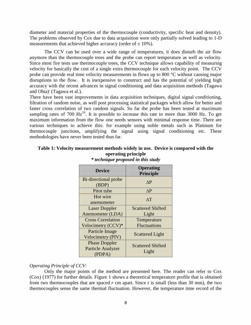
Table 1: Velocity measurement methods widely in use. Device is compared with the

operating principle

* technique proposed in this study

Device Operating

Principle

Bi-directional probe

(BDP) ∆P

Pitot tube ∆P

Hot wire

anemometer ∆T

Laser Doppler

Anemometer (LDA)

Scattered Shifted

Light

Cross Correlation

Velocimetry (CCV)*

Temperature

Fluctuations

Particle Image

Velocimetry (PIV) Scattered Light

Phase Doppler

Particle Analyzer

(PDPA)

Scattered Shifted

Light

Operating Principle of CCV:

Only the major points of the method are presented here. The reader can refer to Cox

(Cox) (1977) for further details. Figure 1 shows a theoretical temperature profile that is obtained

from two thermocouples that are spaced r cm apart. Since r is small (less than 30 mm), the two

thermocouples sense the same thermal fluctuation. However, the temperature time record of the

9

thermocouple located downstream is shifted by a time seconds as shown in Figure 1. If can

be accurately estimated the velocity of the flow is simply given by Eq. 1:

Figure 1: Example of compensated temperature plot from two thermocouples placed r cm

apart. velocity = /r .

/v r . (1)

is determined accurately by using the correlation concept where the degree of association

between certain variables is to be measured (Cox). To calculate the time for a turbulence eddy

passing between the pair of thermocouples the temperature profiles are cross correlated using Eq.

2,

0

1( , ) lim ( ) ( )

T

xyT

R r x t y t dtT

, (2)

Where the two thermocouple signals are represented by x(t) and y(t), and x(t-τ) is the delayed

version of signal x(t). T is the averaging time/sampling period over which the signal is

correlated. Finding the delay between the time when an eddy passes from one thermocouple to

the other requires finding the lag which maximized the correlation function Rxy. To calculate the

time for the turbulence to pass between the two thermocouples the lag is multiplied by the

sampling rate. For the results presented in this paper the averaging time/sampling period was set

to 15 seconds to follow the procedure reported by Motevalli (Motevalli).

CCV is affected by seven main factors: sampling frequency, TC response time, TC separation

distance, turbulent eddy size, soot accumulation, equality of TC time constants, and sampling

period. The two factors examined in this study are frequency and TC separation distance. A

systematic study of the influence of other factors is currently underway at the WPI Fire Science

Laboratory.

Sampling frequency affects the CCV technique because if data is not recorded fast

enough the temperature changes in the turbulent eddies will not be represented correctly by the

temperature profile of each thermocouple. The maximum viable sampling frequency is

determined by the time constant of the thermocouple. This is due to the thermal inertia of the

probe. Sampling to fast will simply result in longer data profiles with no increase in accuracy.

Using a lumped analysis the time constant for a thermocouple is determined from Eq. 3. This is

valid due to the small point like nature of the thermocouples being used (Motevalli).

30 30.2 30.4 30.6 30.8 31 31.20.2

0.3

0.4

0.5

0.6

0.7

0.8

0.9

T/To

Time (s)

Thermocouple #1

Thermocouple #2

30 30.2 30.4 30.6 30.8 31 31.20.2

0.3

0.4

0.5

0.6

0.7

0.8

0.9

T/To

Time (s)

30 30.2 30.4 30.6 30.8 31 31.20.2

0.3

0.4

0.5

0.6

0.7

0.8

0.9

T/To

Time (s)

Thermocouple #1

Thermocouple #2

10

hA

Vc p

R

(3)

The TC response time can be changed by adjusting the size of the thermocouple bead, using

materials with smaller specific heats such as noble metals, or using materials with smaller

densities. Type E type thermocouples are used because of they have the highest output per

degree temperature change of standard thermocouples (approximately 60mV/°C and temperature

range between -270 to 1100°C ). The optimum spacing of the two thermocouples is a function of

the flow velocity due to several factors. First if the TC’s are too far apart the eddy will shift

between the TC’s, secondly if the thermocouples are too close together the downstream

thermocouple will be in the wake of the upstream TC. Also, at smaller spacing’s small errors in

the lag spacing calculation results in large errors in the velocity calculation when the separation

distance is small. The size of the turbulent eddy plays a significant role in the probe accuracy.

According to Motevalli (Motevalli) the accuracy of the CCV technique increases as eddies

become larger and stronger. Changes in bead diameter can be caused by soot accumulation on

the probe. This will affect the time constant of the probe and could make it respond to slowly to

make accurate velocity measurements. If soot builds up unevenly on the two probes then their

respective time constants will become different due to the change in size and thermal mass. If the

two thermocouples have different response times the lag calculated will result in the measured

velocity being to low or to high depending on which TC has the increased response time

(Motevalli). The sampling period can affect the accuracy of the CCV technique. To measure the

most accurate flow profile the sampling period should be long enough to identify the lag in the

signal but short enough to show changes in the flow velocity. The sampling period will

determine the speed at which real time measurements can be updated using this technique.

In a real fire scenario, turbulent eddies are generated by the buoyant entrainment of the

fire itself. In a forced flow jet, as used in this study, the turbulence must be induced and can be

controlled through the use of either obstructions in the flow or a mesh put over the turbulent jet.

For an obstruction in the flow the size and shape are the critical parameters to determine the eddy

size and for a mesh the spacing between wires will determine the eddy size.

This study examines the effects of sampling frequency and thermocouple separation

distance on the CCV technique. By using a heated axisymmetric jet and taking measurements

along the vertical axis these parameters can be adjusted to test their influence on velocity

measurements separately. Measurements from a hot wire anemometer is taken as the true flow

speed and used to calculate the error in the CCV technique.

Experimental Setup:

The experimental setup comprises of a variable speed heated axisymmetric jet

surrounded by a Plexiglas cage. The temperature is controlled by a rheostat which controls the

current powering two resistance heaters aligned in series inside of the axisymmetric jet. The

amount of air injected into the jet is controlled by a regulator connected to the lab air supply. As

shown in figure 2, a set of E type thermocouples, with bead diameters of 7.62x10-5

m (0.003

inches) are passed through 0.15 m (~6 inches) of ceramic insulation and glued in place. A set of

digital calipers mounted parallel to the jet are used to change the spacing between the probes.

The thermocouple wires are shielded to damp the disturbance caused by the electromagnetic

(EM) fields generated from the heating elements. Since the cross correlation only depends on

the phase of the signal and not on the amplitude, cold junction compensation on the

11

thermocouples is not included. A NI DAQ Data Acquisition system comprised of a NI SCXI-

1000 Chassi, NI SCXI 1600 A/D converter, NI SCXI-1102 amplifier, and a NI SCXI 1301

simultaneously sampling unit is used to sample the data at a rate of 1000 to 3000 Hz. An Omega

PMA-902 hot wire anemometer is used to compare the velocity obtained by CCV technique.

Data is collected at spacing’s of 5, 10, 15, 20, and 25 mm and one minute of data is recorded for

each test. These tests are done at a steady velocity of 1.1 m/s with the upper, stationary

thermocouple, 63 mm from the exit of the jet.

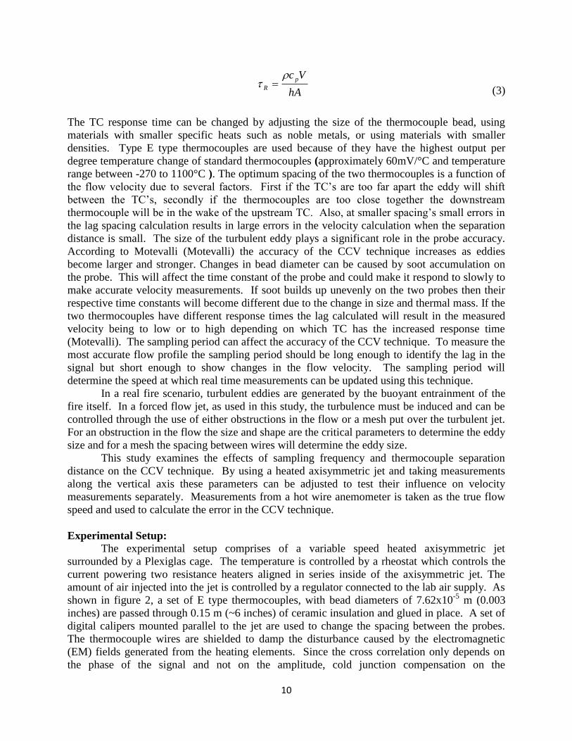
Figure 2: Experimental set up comprising of a heated axisymmetric jet. Two E type

thermocouples with bead diameters of 7.62x10-5

m are shown mounted on a set of digital

calipers to adjust the spacing distance from 5mm to 25mm.

Results and Analysis

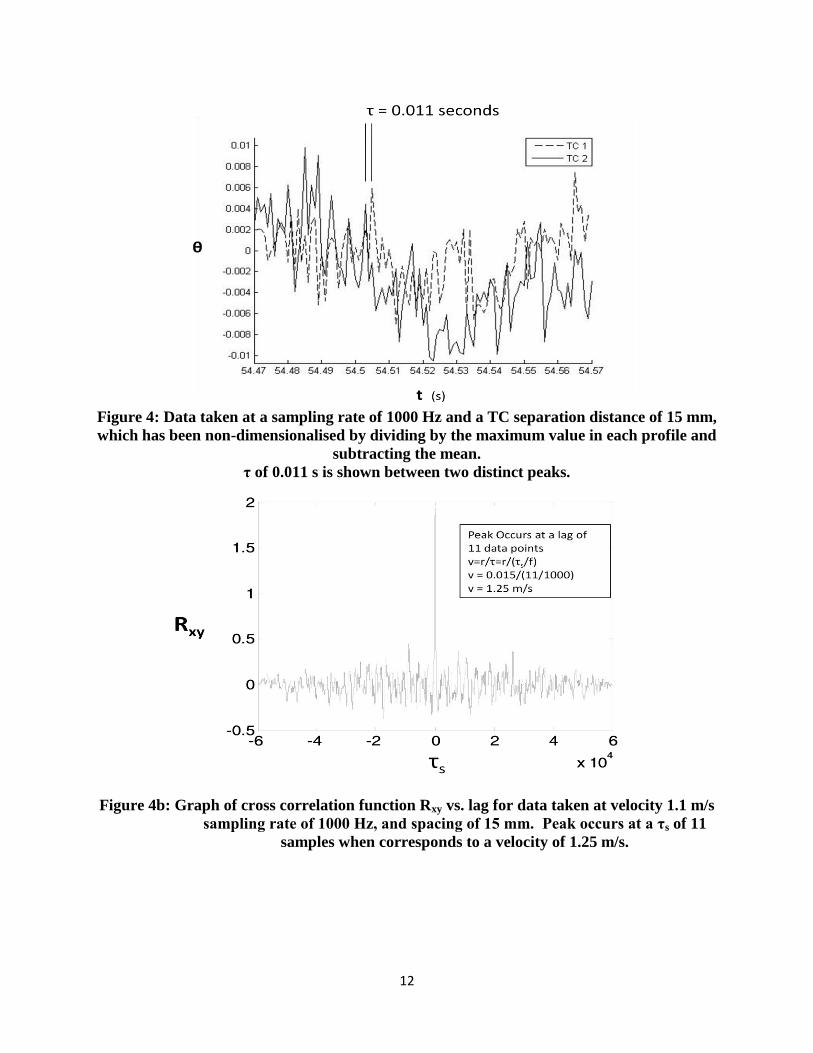
Figure 4 shows part of a non-dimensional adjusted temperature history curve highlighting the

offset of the two temperature profiles. The temperature profiles were nondimensionalized using

Eq. 4 given by,

aveTT

T

max

. (4)

As shown in Figure 4, it is difficult to quantify the lag between two temperature profiles over a

range of temperatures directly necessitating the need to apply a cross correlation to find the

overall lag between two temperature profiles.

Figure 4b shows the results of cross correlating a 15 second set of data taken at a velocity of 1.1

m/s, with a 15mm separation distance between TC probes, and a sampling rate of 1000 Hz. The

cross correlated signal, Rxy has a peak at a lag of 11 data samples which corresponds to a

velocity of 1.25 m/s.

12

Figure 4: Data taken at a sampling rate of 1000 Hz and a TC separation distance of 15 mm,

which has been non-dimensionalised by dividing by the maximum value in each profile and

subtracting the mean.

τ of 0.011 s is shown between two distinct peaks.

Figure 4b: Graph of cross correlation function Rxy vs. lag for data taken at velocity 1.1 m/s

sampling rate of 1000 Hz, and spacing of 15 mm. Peak occurs at a τs of 11

samples when corresponds to a velocity of 1.25 m/s.

13

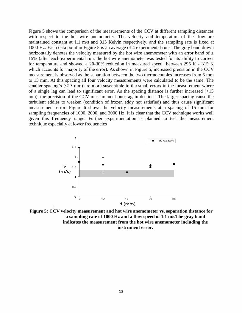
Figure 5 shows the comparison of the measurements of the CCV at different sampling distances

with respect to the hot wire anemometer. The velocity and temperature of the flow are

maintained constant at 1.1 m/s and 313 Kelvin respectively, and the sampling rate is fixed at

1000 Hz. Each data point in Figure 5 is an average of 4 experimental runs. The gray band drawn

horizontally denotes the velocity measured by the hot wire anemometer with an error band of ±

15% (after each experimental run, the hot wire anemometer was tested for its ability to correct

for temperature and showed a 20-30% reduction in measured speed between 295 K - 315 K

which accounts for majority of the error). As shown in Figure 5, increased precision in the CCV

measurement is observed as the separation between the two thermocouples increases from 5 mm

to 15 mm. At this spacing all four velocity measurements were calculated to be the same. The

smaller spacing’s (<15 mm) are more susceptible to the small errors in the measurement where

of a single lag can lead to significant error. As the spacing distance is further increased (>15

mm), the precision of the CCV measurement once again declines. The larger spacing cause the

turbulent eddies to weaken (condition of frozen eddy not satisfied) and thus cause significant

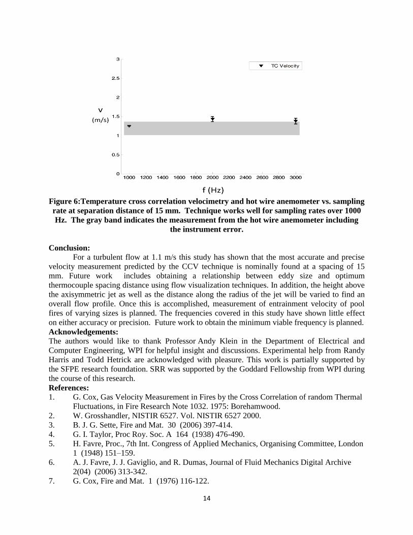
measurement error. Figure 6 shows the velocity measurements at a spacing of 15 mm for

sampling frequencies of 1000, 2000, and 3000 Hz. It is clear that the CCV technique works well

given this frequency range. Further experimentation is planned to test the measurement

technique especially at lower frequencies

.

Figure 5: CCV velocity measurement and hot wire anemometer vs. separation distance for

a sampling rate of 1000 Hz and a flow speed of 1.1 m/sThe gray band

indicates the measurement from the hot wire anemometer including the

instrument error.

14

Figure 6:Temperature cross correlation velocimetry and hot wire anemometer vs. sampling

rate at separation distance of 15 mm. Technique works well for sampling rates over 1000

Hz. The gray band indicates the measurement from the hot wire anemometer including

the instrument error.

Conclusion:

For a turbulent flow at 1.1 m/s this study has shown that the most accurate and precise

velocity measurement predicted by the CCV technique is nominally found at a spacing of 15

mm. Future work includes obtaining a relationship between eddy size and optimum

thermocouple spacing distance using flow visualization techniques. In addition, the height above

the axisymmetric jet as well as the distance along the radius of the jet will be varied to find an

overall flow profile. Once this is accomplished, measurement of entrainment velocity of pool

fires of varying sizes is planned. The frequencies covered in this study have shown little effect

on either accuracy or precision. Future work to obtain the minimum viable frequency is planned.

Acknowledgements:

The authors would like to thank Professor Andy Klein in the Department of Electrical and

Computer Engineering, WPI for helpful insight and discussions. Experimental help from Randy

Harris and Todd Hetrick are acknowledged with pleasure. This work is partially supported by

the SFPE research foundation. SRR was supported by the Goddard Fellowship from WPI during

the course of this research.

References:

1. G. Cox, Gas Velocity Measurement in Fires by the Cross Correlation of random Thermal

Fluctuations, in Fire Research Note 1032. 1975: Borehamwood.

2. W. Grosshandler, NISTIR 6527. Vol. NISTIR 6527 2000.

3. B. J. G. Sette, Fire and Mat. 30 (2006) 397-414.

4. G. I. Taylor, Proc Roy. Soc. A 164 (1938) 476-490.

5. H. Favre, Proc., 7th Int. Congress of Applied Mechanics, Organising Committee, London

1 (1948) 151–159.

6. A. J. Favre, J. J. Gaviglio, and R. Dumas, Journal of Fluid Mechanics Digital Archive

2(04) (2006) 313-342.

7. G. Cox, Fire and Mat. 1 (1976) 116-122.

15

8. G. Cox, Comb. and Flame 28 (1977) 155-163.

9. G. Cox and R. Chitty, Comb. and Flame 39 (1980) 191-209.

10. V. Motevalli, C. H. Marks, and B. J. McCaffrey, Journal of Heat Transfer (Transactions

of the ASME (1992)

11. J. L. Dupuy, J. Marechal, L. Bouvier, and N. Lois, Proceedings of 3rd international

conference on forest fire research–14th conference on fire and forest meteorology

(1998) 16–20.

12. J. L. Dupuy, J. Maréchal, and D. Morvan, Comb. and Flame 135(1-2) (2003) 65-76.

13. T. Marcelli, P. A. Santoni, A. Simeoni, E. Leoni, and B. Porterie, International Journal of

Wildland Fire 13 (2004) 37-48.

14. P. A. Santoni, T. Marcelli, and E. Leoni, Comb. and Flame 131(1) (2002) 47-58.

15. M. Tagawa and Y. Ohta, Combust. Flame 109(4) (1997) 549-560.

16. M. Tagawa, K. Kato, and Y. Ohta, Review of Scientific Instruments 74 (2003) 1350.

17. V. Motevalli, A Study of the Characteristics of Small-Scale Unconfined Fire Induced

Ceiling Jets, in ME. 1989, University of Maryland, College Park.

16

Chapter 2:

An Examination of Cross Correlation Velocimetry’s Ability to

Predict Characteristic Turbulent Length Scales in Fire Induced

Flow

Presented at the 2009 Fall Technical Meeting Organized by the Eastern States Section of the

Combustion Institute

S. Rockwell,1 A. Rangwala,

1 and A. Klein

2

1Department of Fire Protection Engineering, Worcester Polytechnic Institute,

Worcester, Massachusetts 01609, USA

2 Department of Electrical and Computer Engineering, Worcester Polytechnic Institute

Worcester, Massachusetts 01609, USA

Since the early 1970’s Cross Correlation Velocimetry (CCV) has been used to measure velocity of

turbulent flows. This study explores the use of the cross correlation coefficient decay towards

estimation of characteristic turbulent length scales typically found in a fire. To test the theory,

experiments were performed in a turbulent free jet and a natural gas fire plume. The experiments

showed that CCV measurements were comparable to the velocity decay obtained using Laser

Doppler Anemometer (LDA). Ultimately, a prototype probe was developed that could measure

temperature, velocity, and flow width simultaneously in the plume of a natural gas burner. This

allows for a direct estimation of the mass flow in a fire plume.

1. Introduction

Quantitative flow measurements in fires are difficult due to the extreme temperatures and

density variations in both amplitude and frequency occurring in fire flows (Tieszen 2001).

Normally a fire flow’s width is determined by making multiple measurements along the width of

either velocity or temperature, and estimating where the measured parameter decays to a minimal

value. This study discusses the creation of a probe using Cross Correlation Velocimetry (CCV),

known as a triple CCV probe, capable of simultaneously measuring the temperature, velocity,

and flow width from a single measurement. The dependence of the probe on sampling frequency

and sampling time are presented. This probe can be used to estimate a fire’s plume width and

possibly the ceiling jet thickness caused by a compartment fire. Measurement of fire plume

temperature, velocity, and width also allows for the direct calculation of the fire’s mass flux into

the upper hot layer in a compartment fire. Characterization of ceiling jet thickness is important in

the analysis of sprinkler activation, flashover calculations, and tenability/egress analysis in

compartment fires that occur in, for example, structural and tunnel fires.

2. Operating Principle and Theoretical Background:

CCV uses temperature-time records from a set of thermocouples, one downstream of the

other, cross-correlated to determine the flow's velocity similar to spatial and drift cross-

correlation velocimetry (Morgan and Bowles 1968; Marvasti and Strahle 1994). The CCV

17

technique uses the inherent turbulent structures generated by fire flows as the tracers to follow

the bulk flow. CCV is based on the “frozen eddy” concept in turbulent flows proposed by Taylor

in 1938 (Taylor 1938). Taylor hypothesized that in a turbulent flow, there are random and unique

eddy structures that retain their shape and characteristics over some small time and space. This

concept is analogous to performing a numerical integration of a function over a small interval. In

between 1975 and 1980 Cox et al. (Cox 1976; Cox and Chitty 1980) performed a series of

experiments that verified the “frozen eddy” hypothesis in a non-isotropic ceiling-jet flow

showing velocity measurements could be achieved by means of CCV and thus developing the

one dimensional CCV probe. The velocity u of a flow can be calculated using (Cox 1975),

du , (1)

where d is the thermocouple separation distance in the direction of the flow and τ is the time lag

(s) between the two thermocouple signals. Figure 1 shows an example of a turbulent jet with a

dual CCV probe and sample temperature profile outputs.

Experimental measurements include signal noise and dissipation of small eddy structures

which make the measurement of τ more difficult. To measure τ in a signal with noise, in which a

visual measurement is not possible, the time lag τ can be calculated using,

f

sN , (2)

where τsN is the nominal sampling lag, or the number of data samples the second signal is

delayed behind the first, and f is the sampling frequency. τsN is found by calculating at what lag

the non-dimensional cross coefficient ρxy has a maximum as shown in figure 2. To make the

thermocouple data easier to manage numerically, the temperature profiles are normalized using,

maxT

TT avgs , (3)

where Ts is the measured temperature, Tavg is the mean temperature of the data set, and Tmax is the

maximum temperature in the data set. The nondimensionalized cross correlation coefficient ρxy

can be calculated using,

5.025.02

0

)()(

)()(1

lim

zz

dtzzT

ysx

T

ysxT

xy

, (4)

where z is the position in the temperature profile, τs is the sampling lag, T is the total number of

samples, and 𝜃x(z) and 𝜃y(z) represent the normalized first and second temperature readings

respectively. By plotting ρxy verses τs the nominal sampling lag τsN is found as the abscissa of the

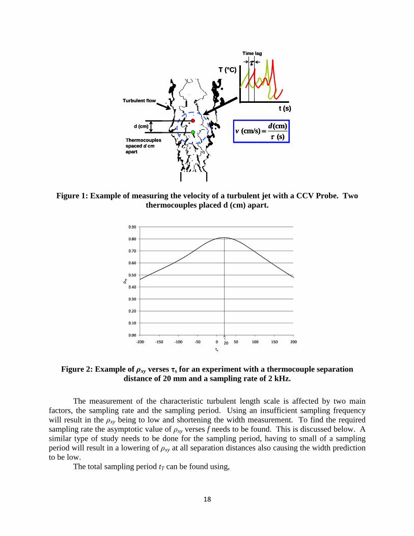
peak. Figure 2 shows an example of ρxy verses τs plot using a f of 2 kHz and a d of 20 mm where

the τsN is 20 which corresponds to a velocity of 2 m/s using Eqs. 1 and 2.

Signals with a strong correlation have a ρxy close to unity while signals with a weak

correlation have lower values of ρxy. Motevalli (Motevalli 1989) reported that ρxy > 0.5 is needed

for an accurate velocity measurement. This makes intuitive sense because ρxy above 0.5 implies

greater confidence in the statistical similarity of the signals where as if ρxy is below 0.5 then it is

more likely that the two signals are unrelated. Further discussion on the velocity, temperature

measurement capabilities of CCV, and the practical considerations for the cross correlation

technique are discussed elsewhere (Cox ; Motevalli, Marks et al.), (Wills 1964).

18

Figure 1: Example of measuring the velocity of a turbulent jet with a CCV Probe. Two

thermocouples placed d (cm) apart.

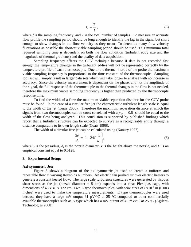
Figure 2: Example of ρxy verses τs for an experiment with a thermocouple separation

distance of 20 mm and a sampling rate of 2 kHz.

The measurement of the characteristic turbulent length scale is affected by two main

factors, the sampling rate and the sampling period. Using an insufficient sampling frequency

will result in the ρxy being to low and shortening the width measurement. To find the required

sampling rate the asymptotic value of ρxy verses f needs to be found. This is discussed below. A

similar type of study needs to be done for the sampling period, having to small of a sampling

period will result in a lowering of ρxy at all separation distances also causing the width prediction

to be low.

The total sampling period tT can be found using,

Turbulent flow

T (°C)

t (s)

Time lag

(cm) (cm/s)

(s)

dv

d (cm)

Thermocouples

spaced d cm

apart

Turbulent flow

T (°C)

t (s)

Time lag

(cm) (cm/s)

(s)

dv

d (cm)

Thermocouples

spaced d cm

apart

19

f

TtT , (5)

where f is the sampling frequency, and T is the total number of samples. To measure an accurate

flow profile the sampling period should be long enough to identify the lag in the signal but short

enough to show changes in the flow velocity as they occur. To detect as many flow velocity

fluctuations as possible the shortest viable sampling period should be used. This minimum total

required sampling time is dependent on both the flow condition (turbulent eddy size and the

magnitude of thermal gradients) and the quality of data acquisition.

Sampling frequency affects the CCV technique because if data is not recorded fast

enough the temperature changes in the turbulent eddies will not be represented correctly by the

temperature profile of each thermocouple. Due to the thermal inertia of the probe the maximum

viable sampling frequency is proportional to the time constant of the thermocouple. Sampling

too fast will simply result in larger data sets which will take longer to analyse with no increase in

accuracy. Since the velocity measurement is dependent on the phase, and not the amplitude of

the signal, the full response of the thermocouple to the thermal changes in the flow is not needed,

therefore the maximum viable sampling frequency is higher than predicted by the thermocouple

response time.

To find the width of a flow the maximum viable separation distance for the CCV probe

must be found. In the case of a circular free jet the characteristic turbulent length scale is equal

to the width of the jet (Turns 2000). Therefore the maximum separation distance at which the

signals from two thermocouples can be cross correlated with a ρxy = 0.5 should be equal to the

width of the flow being analyzed. This conclusion is supported by published findings which

report that a turbulent structure can be expected to survive as a recognizable entity through a

distance comparable to its own length scale (Coats 1996).

The width of a circular free jet can be calculated using (Kanury 1977),

ii d

xC

d241

2, (6)

where δ is the jet radius, di is the nozzle diameter, x is the height above the nozzle, and C is an

empirical constant equal to 0.0128.

3. Experimental Setup:

Axi-symmetric Jet:

Figure 3 shows a diagram of the axi-symmetric jet used to create a uniform and

repeatable flow at varying Reynolds Numbers. An electric fan pushed air over electric heaters to

generate a constant heated flow. The large scale turbulence structures were generated by viscous

shear stress as the jet (nozzle diameter = 5 cm) expands into a clear Plexiglas cage, with

dimensions of 46 x 46 x 122 cm. Two E type thermocouples, with wire sizes of 8x10-5

m (0.003

inches) were used to make the temperature measurements. E type thermocouples were used

because they have a large mV output 61 μV/°C at 25 °C compared to other commercially

available thermocouples such as K type which has a mV output of 40 mV/°C at 25 °C (Agilent-

Technologies 2008).

20

Figure 3: Axi-symmetric jet experimental setup

To confirm that the thermocouples had similar response times the probes were reversed

in a constant flow and comparable results were obtained. The separation distance between

thermocouples could be varied with accuracy up to 0.01 mm in the flow while keeping the

measurement volume at the same height above the jet nozzle. In the vertical plane the

thermocouples were aligned using a laser-based alignment system which decreased the error due

to misalignment. Thermocouple measurements were recorded by a NI DAQ data acquisition. An

intelligent Laser Applications (ILA) 75 mW fixed optical path length fp50-shift LDA system

was used as the reference velocity measurement.

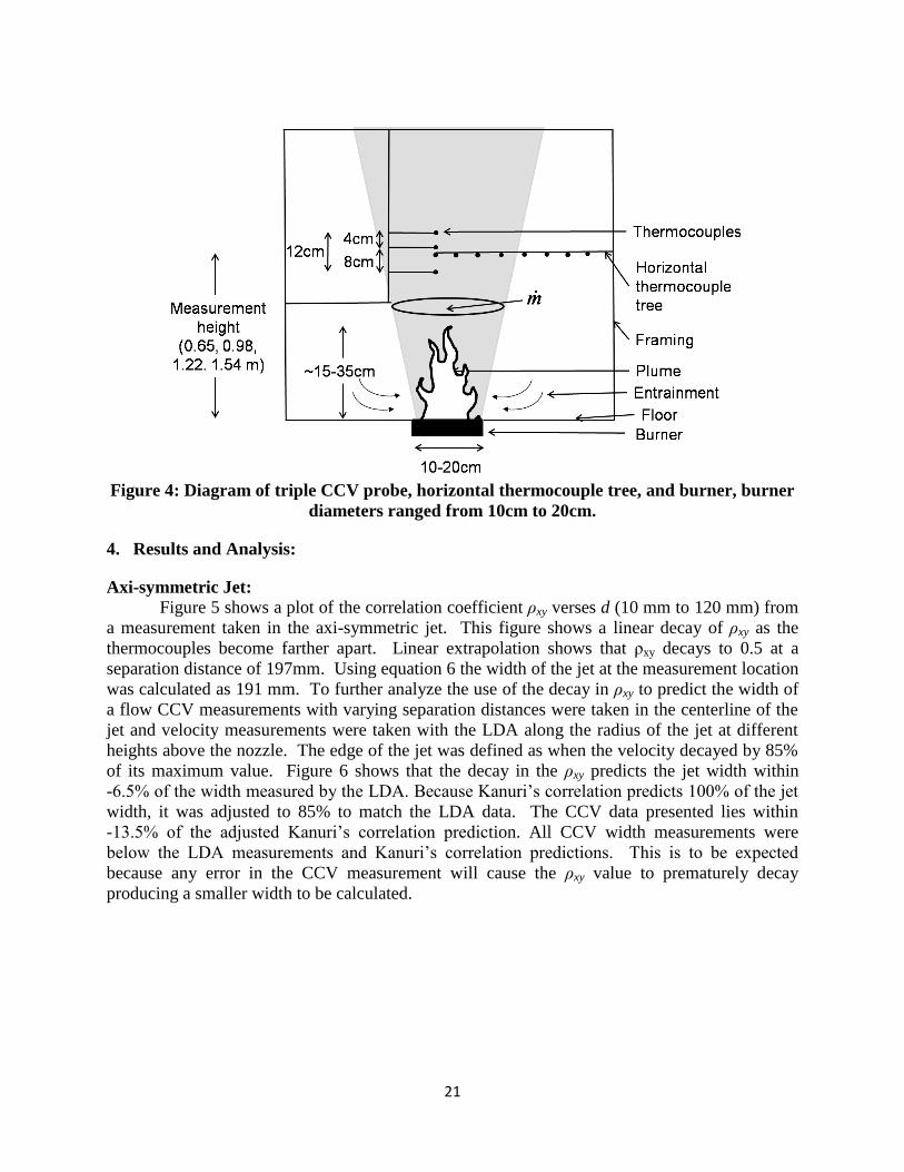
Natural Gas burner:

A natural gas burner was built to test the tipple CCV probe’s ability to work in a real fire

scenario. The burner was built with a 1.22 m by 1.22 m square drywall top with a sand burner in

the middle. This tabletop design kept the air entrainment horizontal at the fire’s base. The

diameter of the burner was adjusted by attaching a steel plate with a hole equal to the desired

burner size. Fires having base diameters of 10 cm, 15 cm, and 20 cm and heat release rates

between 6.2 kW and 23.7 kW were tested. The heat release rate was determined by adjusting the

flow of natural gas to the burner. Measurements were taken at 4 heights above the plume (0.65m

0.98m, 1.22m, 1.54m). A triple thermocouple probe as shown in figure 4 was built to measure

temperature, velocity and plume width simultaneously. The triple CCV probe had separation

distances of 4 cm, and 8 cm providing 3 total separation distances (4, 8, and 12cm) with which to

calculate the ρxy decay. The same E type thermocouples used in the Axi-symmetric jet were used

here as-well. The thermocouples were aligned in the vertical direction using a plumb bob before

each test. To compare with the measurement of CCV probe the plume width was measured

using a horizontal thermocouple tree of eight E type thermocouples as shown in figure 4. To

find the point of 85% decay in the temperature profile these eight measurements were fitted to a

fifth order polynomial which was solved for the desired loss. Due to the low temperatures at the

heights above the plume tested radiation loss incurred a maximum of 0.8% error in the

calculation of the width of the plume and was not included.

21

Figure 4: Diagram of triple CCV probe, horizontal thermocouple tree, and burner, burner

diameters ranged from 10cm to 20cm.

4. Results and Analysis:

Axi-symmetric Jet:

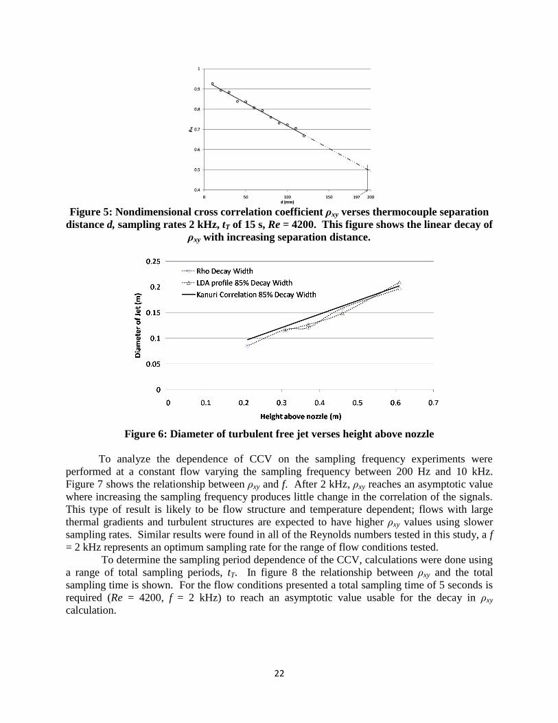
Figure 5 shows a plot of the correlation coefficient ρxy verses d (10 mm to 120 mm) from

a measurement taken in the axi-symmetric jet. This figure shows a linear decay of ρxy as the

thermocouples become farther apart. Linear extrapolation shows that ρxy decays to 0.5 at a

separation distance of 197mm. Using equation 6 the width of the jet at the measurement location

was calculated as 191 mm. To further analyze the use of the decay in ρxy to predict the width of

a flow CCV measurements with varying separation distances were taken in the centerline of the

jet and velocity measurements were taken with the LDA along the radius of the jet at different

heights above the nozzle. The edge of the jet was defined as when the velocity decayed by 85%

of its maximum value. Figure 6 shows that the decay in the ρxy predicts the jet width within

-6.5% of the width measured by the LDA. Because Kanuri’s correlation predicts 100% of the jet

width, it was adjusted to 85% to match the LDA data. The CCV data presented lies within

-13.5% of the adjusted Kanuri’s correlation prediction. All CCV width measurements were

below the LDA measurements and Kanuri’s correlation predictions. This is to be expected

because any error in the CCV measurement will cause the ρxy value to prematurely decay

producing a smaller width to be calculated.

22

Figure 5: Nondimensional cross correlation coefficient ρxy verses thermocouple separation

distance d, sampling rates 2 kHz, tT of 15 s, Re = 4200. This figure shows the linear decay of

ρxy with increasing separation distance.

Figure 6: Diameter of turbulent free jet verses height above nozzle

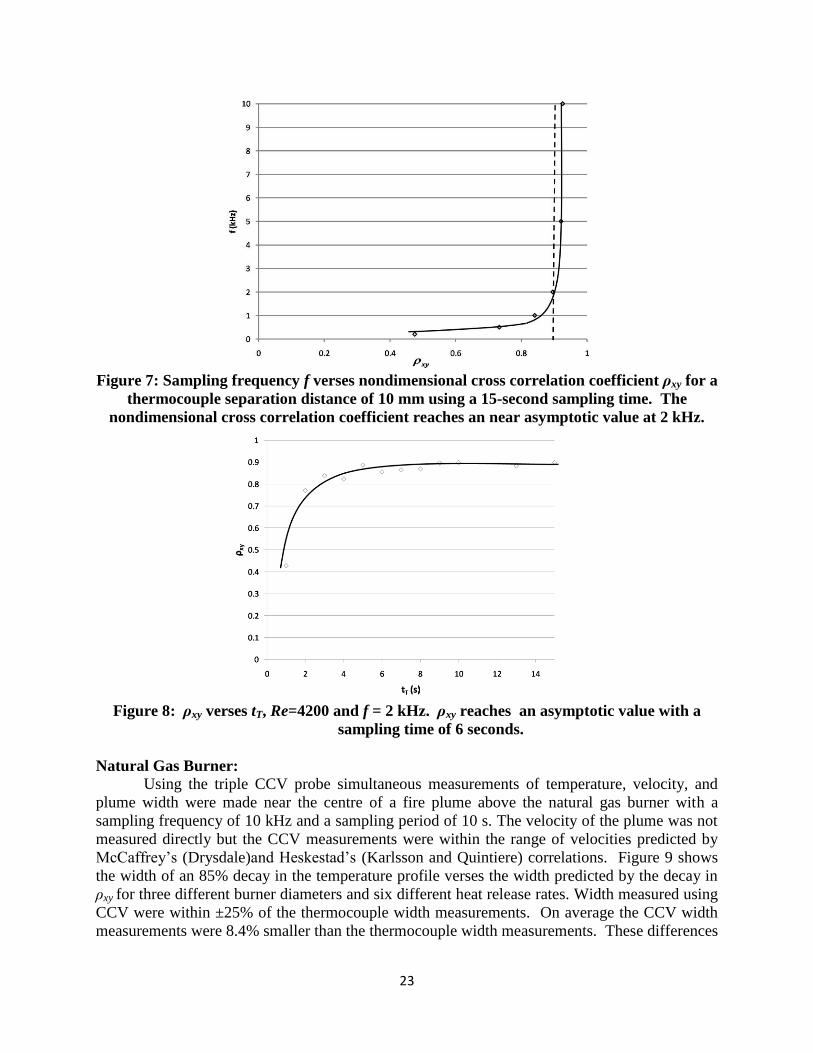
To analyze the dependence of CCV on the sampling frequency experiments were

performed at a constant flow varying the sampling frequency between 200 Hz and 10 kHz.

Figure 7 shows the relationship between ρxy and f. After 2 kHz, ρxy reaches an asymptotic value

where increasing the sampling frequency produces little change in the correlation of the signals.

This type of result is likely to be flow structure and temperature dependent; flows with large

thermal gradients and turbulent structures are expected to have higher ρxy values using slower

sampling rates. Similar results were found in all of the Reynolds numbers tested in this study, a f

= 2 kHz represents an optimum sampling rate for the range of flow conditions tested.

To determine the sampling period dependence of the CCV, calculations were done using

a range of total sampling periods, tT. In figure 8 the relationship between ρxy and the total

sampling time is shown. For the flow conditions presented a total sampling time of 5 seconds is

required (Re = 4200, f = 2 kHz) to reach an asymptotic value usable for the decay in ρxy

calculation.

23

Figure 7: Sampling frequency f verses nondimensional cross correlation coefficient ρxy for a

thermocouple separation distance of 10 mm using a 15-second sampling time. The

nondimensional cross correlation coefficient reaches an near asymptotic value at 2 kHz.

Figure 8: ρxy verses tT, Re=4200 and f = 2 kHz. ρxy reaches an asymptotic value with a

sampling time of 6 seconds.

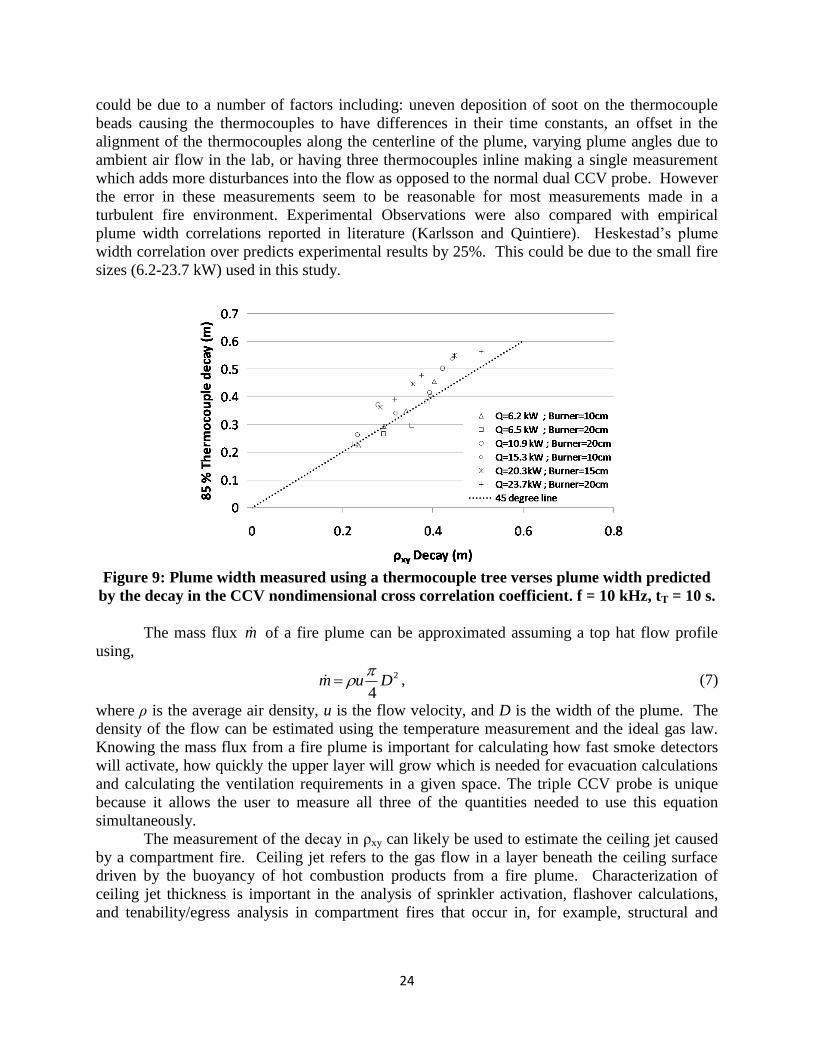
Natural Gas Burner:

Using the triple CCV probe simultaneous measurements of temperature, velocity, and

plume width were made near the centre of a fire plume above the natural gas burner with a

sampling frequency of 10 kHz and a sampling period of 10 s. The velocity of the plume was not

measured directly but the CCV measurements were within the range of velocities predicted by

McCaffrey’s (Drysdale)and Heskestad’s (Karlsson and Quintiere) correlations. Figure 9 shows

the width of an 85% decay in the temperature profile verses the width predicted by the decay in

ρxy for three different burner diameters and six different heat release rates. Width measured using

CCV were within ±25% of the thermocouple width measurements. On average the CCV width

measurements were 8.4% smaller than the thermocouple width measurements. These differences

24

could be due to a number of factors including: uneven deposition of soot on the thermocouple

beads causing the thermocouples to have differences in their time constants, an offset in the

alignment of the thermocouples along the centerline of the plume, varying plume angles due to

ambient air flow in the lab, or having three thermocouples inline making a single measurement

which adds more disturbances into the flow as opposed to the normal dual CCV probe. However

the error in these measurements seem to be reasonable for most measurements made in a

turbulent fire environment. Experimental Observations were also compared with empirical

plume width correlations reported in literature (Karlsson and Quintiere). Heskestad’s plume

width correlation over predicts experimental results by 25%. This could be due to the small fire

sizes (6.2-23.7 kW) used in this study.

Figure 9: Plume width measured using a thermocouple tree verses plume width predicted

by the decay in the CCV nondimensional cross correlation coefficient. f = 10 kHz, tT = 10 s.

The mass flux m of a fire plume can be approximated assuming a top hat flow profile

using,

2

4Dum

, (7)

where ρ is the average air density, u is the flow velocity, and D is the width of the plume. The

density of the flow can be estimated using the temperature measurement and the ideal gas law.

Knowing the mass flux from a fire plume is important for calculating how fast smoke detectors

will activate, how quickly the upper layer will grow which is needed for evacuation calculations

and calculating the ventilation requirements in a given space. The triple CCV probe is unique

because it allows the user to measure all three of the quantities needed to use this equation

simultaneously.

The measurement of the decay in ρxy can likely be used to estimate the ceiling jet caused

by a compartment fire. Ceiling jet refers to the gas flow in a layer beneath the ceiling surface

driven by the buoyancy of hot combustion products from a fire plume. Characterization of

ceiling jet thickness is important in the analysis of sprinkler activation, flashover calculations,

and tenability/egress analysis in compartment fires that occur in, for example, structural and

25

tunnel fires. Figures 10a and 10b show diagrams of a typical ceiling jet generated by a fire at the

back of a room and the expansion of a circular free jet respectively.

Figure 10: Application of CCV to measure characteristic turbulent length scales. (a)

Typical ceiling jet found in a compartment fire. (b) Axi-symmetric free jet

5. Conclusions

The triple CCV probe can measure the temperature, velocity, and characteristic turbulent

length scale of a medium to high temperature turbulent flow which allows the direct calculation

of a fire plumes mass flux. The CCV’s width measurement is most effected by 2 main factors,

sampling frequency and sampling time. For different types of flow conditions in which these

measurements are done an analysis to find the asymptotic value for these two parameters is

required. For the flows tested here, the minimum required sampling time was found to be 5

seconds and the optimum sampling frequency was found to be 2 kHz.

In the future this technique could be used to measure the ceiling jet thickness in

compartment fires. Future work is needed to characterize the angular dependence of this

measurement, how far away from the centre of the plume the thermocouple sensor can be placed

before an accurate measurement of the plume width is no longer possible, and how close to the

characteristic turbulent length scale the thermocouple separation distance can be and still make a

valid measurement. These parameters are important for using the triple CCV probe to measure

the ceiling jet thickness.

Acknowledgments

The help of laboratory manager Randy Harris is acknowledged. This work was partially funded

by the Society of Fire Protection Engineering (SFPE) Education and Scientific Foundation

Grant. The research is currently funded through the National Science Foundation (NSF)

Graduate Research Fellowship Program (GRFP).

References

1. Tieszen, S.R., On the Fluid Mechanics of Fires. Annual Rev. Fluid Mech., 2001. 33: p.

67-92.

26

2. Marvasti, M.A. and W.C. Strahle, Fractal interpolation methods in spatial cross-

correlation velocimetry. Experiments in Fluids, 1994. 18: p. 129-130.

3. Morgan, M.G. and K.L. Bowles, Cross-Correlation and Cross-Spectral Methods for Drift

Velocity Measurements. Science, 1968. 161(3846): p. 1139-1142.

4. Taylor, G.I., The Spectrum of Turbulence. Proc Roy. Soc. A, 1938. 164: p. 476-490.

5. Cox, G., Some Measurements of Fire Turbulence. Fire and Mat., 1976. 1: p. 116-122.

6. Cox, G. and R. Chitty, Study of the Deterministic Properties of Unbounded Fire Plumes.

Comb. and Flame, 1980. 39: p. 191-209.

7. Cox, G., Gas Velocity Measurement in Fires by the Cross Correlation of random

Thermal Fluctuations, in Fire Research Note 1032. 1975: Borehamwood.

8. Motevalli, V., A Study of the Characteristics of Small-Scale Unconfined Fire Induced

Ceiling Jets, in ME. 1989, University of Maryland, College Park.

9. Cox, G., Gas Velocity Measurements in Fires by the Cros-Correlation of Random

Thermal Fluctuations- A Comparison with Conventional Techniques. Comb. and Flame,

1977. 28: p. 155-163.

10. Motevalli, V., C.H. Marks, and B.J. McCaffrey, Cross-correlation velocimetry for

measurement of velocity and temperature profiles in low-speed, turbulent, nonisothermal

flows. Journal of Heat Transfer (Transactions of the ASME), 1992.

11. Wills, J.A.B., On Convection Velocities in turbulent Shear Flows. Journal of Fluid

Mechanics, 1964. 20(3): p. 417-432.

12. Turns, S.R., An Introduction to Combustion: Concepts and Applications. 2000, New

York: McGraw Hill.

13. Coats, C.M., Coherent Structures in Combustion. Prog. Energy Combustion Science,

1996. 22: p. 427-509.

14. Kanury, A.M., An Introduction to Combustion Phenomena. 1977: Gordon & Breach

Science Publishers, Inc.

15. Technologies, A., Application Notes - Practical Temperature Measurements. 2008: USA.

p. 11.

16. Drysdale, D., An Introduction to Fire Dynamics. 1999: John Wiley & Sons.

17. Karlsson, B. and J.G. Quintiere, Enclosure Fire Dynamics. 2000: CRC Press.

27

Chapter 3: Cross Correlation Velocimetry in Turbulent Fire-Induced Flows

S. Rockwell1, A. Klein

2, and A. S. Rangwala

1

1Department of Fire Protection Engineering,

2Department of Electrical and Computer Engineering

103 Higgins Lab, 100 Institute Rd, Worcester Polytechnic Institute

Worcester, MA 01609

1. Abstract

This study analyses the applicability of cross correlating the signal between two thermocouples

to obtain simultaneous measurement of velocity, integral turbulent length scales, and temperature

in fire induced turbulent flows. This sensor is based on the classical Taylor’s hypothesis which

states that turbulent structures should retain their shape and identity over a small period of time.

If sampling rate is fast enough such that the signal from two thermocouples is sampled within

this time duration, the turbulent eddy can be used as a tracer to measure flow velocity and

fluctuation. Experiments performed in two laboratory scale devices: a heated turbulent jet and a

variable diameter natural gas burner show that sampling rate, sampling time, and angular

orientation with respect to the bulk flow are the most sensitive parameters in velocity

measurements. Flows with Reynolds numbers between 300 (u=0.1m/s) and 6000 (u=2.0 m/s)

were tested.

2. Nomenclature: BDP = Bi-directional probe

C = Empirical constant (-)

CCV = Cross Correlation Velocimetry

d = Distance between thermocouples (mm)

di = Nozzle exit diameter (m)

dP = Diameter of seed particles (m)

f = Sampling frequency (Hz)

fτ = Maximum sampling frequency using full thermocouple response (Hz)

fR = Maximum sequential sampling rate (Hz)

LDA = Laser Doppler Anemometer

PIV = Particle Image Velocimetry

Re = Reynolds number (-)

t = Time (s)

tT = Total sampling time (s)

t1 = Air transition time (s)

t2 = Overlap time (s)

tTR = Total required sampling time (s)

T = Temperature (°C)

T = Total number of samples (-)

u = Velocity (m/s)

urel = Seed particle relative velocity (m/s)

28

Vm = Measured Velocity

VT = Total bulk flow Velocity

x = Distance away from nozzle (m)

z = Position in array ( - )

Greek:

ρ = Fluid density (kg/m3)

ρP = Density of seed particles (kg/m3)

ρf = Density of fluid (kg/m3)

ρxy = Non-dimensional cross correlation coefficient (-)

θ = Normalized temperature (-)

τ = Time lag (s)

τs = Sampling lag (-)

τsN = Nominal sampling lag (-)

τR = Response time (s)

δ = ½ Plume width (m)

v = Kinematic viscosity (m2/s)

μ = Viscosity (N s/m2)

Subscripts:

max = Maximum in data set

avg = Average of data set

m = Measured

c = Corrected

3. Introduction:

Accurate measurements of temperature and velocity fields created by fire plumes are vital in

quantifying the thermal impact of a fire. Knowledge of these high temperature flows play a

major role in the prediction of ceiling jet velocity, smoke detector, and sprinkler activation,

requirements for smoke venting systems, and estimation of available safe egress times (ASET).

Recent large scale experimental studies on fires in building have discussed the lack of accurate

velocity measurement techniques in fires and the severe need of research in this area (Torero and

Carvel 2007).

Quantitative flow measurements in fires are difficult due to the elevated temperatures and

caustic environment in fire flows (Tieszen 2001). This causes any kind of sensitive instrument

difficult to maintain. Table 1 shows velocity measurement techniques currently in use along

with their cost and accuracy. The bi-directional probe (BDP) is predominantly used to make

measurements in full-scale fire experiments (Bryant 2009). The BDP calculates velocity by

comparing the pressure difference between the stagnation pressure on the upstream portion and

the static pressure in the downstream portion of the probe. The BDP has difficulty resolving

velocities below 0.3 m/s accurately (McCaffrey and Heskestad 1976). This type of probe also

uses a correction factor which changes with variation in the pitch and yaw angles3 (Sette 2006).

The pitot tube works in a similar fashion to the BDP but it uses small pressure ports which can

become clogged with combustion products (Koslowski 1991; Sette 2006). The hot wire

3 Pitch and yaw are changes in the vertical and horizontal axis of the probe with respect to the bulk flow direction.

29

anemometer, works well for ambient temperature flows; however, the accuracy and robustness of

the probe drops with changing elevated temperatures. The Laser Doppler Anemometer (LDA) is

non-intrusive and has better spatial resolution than a hot wire anemometer but requires seeding

of the flow (Degraaff and Eaton 2001). Particle Image Velocimetry (PIV) is also highly

dependent on particle seeding (Astarita 2008). These laser based systems work well for

measuring bench scale experimental flows but both seeding and recording the reflection of laser

light from the seed particles is difficult in full scale fire situations. Laser systems are also

prohibitively expensive and many use a class 4 laser which must be contained to prevent

optically damaging transmission from exiting the experiment.

A velocity probe using the cross correlation velocimetry (CCV) technique separates itself

from these traditional techniques because it is inexpensive, easy to operate, robust, and capable

of measuring low speed flows. This study discusses the frequency, sampling time, spatial

dependence, and angular dependence of CCV technique towards the creation of a functional

sensor. This study also presents a method for estimating the integral turbulent length scales in

turbulent flow using the CCV technique which was used to measure a fire plume width which

might be used to measure ceiling jet thickness in a developing compartment fire. The integral

length scale is vital to optimize grid scale resolution for use with Large Eddy Simulation (LES)

computational fluid dynamic (CFD) models. In CFD models two equation models are often used

known as the k-ε turbulence model. The dissipation rate ε is a strong function of the integral

length scale. It is always assumed that the integral length scale is finite (Tennekes and Lumley

1972). Experimentally the integral length scale can be defined as the length beyond which fluid

mechanical quantities become uncorrelated (Glassman 1996). This occurs when eddies are of

the order of the width of the shear flow, for example the diameter of a pipe or the width of a

boundary layer along a wall (Kundu and Cohen 1987) similar to a ceiling jet in a developing

compartment fire.

CCV uses temperature-time records from a set of thermocouples, one downstream of the

other, cross-correlated to determine the flow's velocity similar to spatial and drift cross-

correlation velocimetry (Morgan and Bowles 1968; Marvasti and Strahle 1994). This technique

based on the “frozen eddy” concept in turbulent flows proposed by Taylor in 1938 (Taylor 1938)

where he hypothesized that in a turbulent flow, there are random and unique eddy structures that

retain their shape and characteristics over some time and space. This concept is analogous to

performing a numerical integration of a function over a small interval. Several Studies in fluid

mechanics have shown the validity of this assumption (Antonia et al. 1979; Cenedese et al. 1991;

Burghelea et al. 2005). Investigations of turbulent flows have shown the movement of eddy

structures to be a good representation of the true mean flow velocity (Dupuy, Marechal et al.

2003; Favre, Gaviglio et al. 2006). In between 1975 and 1980 Cox et al. (Cox 1976; Cox and

Chitty 1980) performed a series of experiments that verified the “frozen eddy” hypothesis in a

non-isotropic ceiling-jet flow showing velocity measurements could be achieved by means of

CCV and thus developing the one dimensional CCV probe. Non-isotropy is necessary, because

temperature records are used to capture the flow velocity. Thus it is assumed that there is

proportionality between the fluctuating velocity and temperature field in a turbulent flow.

Interestingly, for the current set of experiments we show that this proportionality is linear. This is

discussed further in the results and analysis section.

Due to the high cost associated with analogue correlators available in the 1970’s, the

CCV technique phased out after the advent of the bidirectional probe which was significantly

cheaper at that time. This technique had been used more recently in fire related research by

30

Motevalli et al. (Motevalli 1989; Motevalli, Marks et al. 1992), Marrion (Marrion 1989) and

Dupuy et al. (Dupuy, Marechal et al. 2003). This work further established limitations associated

with the sampling frequency and the time constant of the thermocouple. The problems observed

by Cox (Cox 1976) due to data acquisition were partially solved leading to 1-D measurements

that achieved higher accuracy (order of ± 5%). The current is different from prior work in this

area because it investigates higher sampling rates (up to 10 kHz), wider range of velocities (0.1 –

2 m/s), and thoroughly investigates the sampling time requirements to apply this technique in the

field. In addition, this work also investigates the applicability of using CCV to obtain

information on the characteristic of the turbulent flow. As a first step, a methodology to predict

integral turbulent length scales is presented.

4. Operating Principle:

Figure 1 shows an illustrative sketch of a heated turbulent flow where two thermocouples are

used to measure velocity. The velocity u (m/s) of a flow can be calculated using (Cox 1975),

du , (1)

where d (m) is the thermocouple separation distance and τ is the time lag (s) between the two

thermocouple signals. In practice, the thermocouple separation distance is a known quantity. The

time lag can be measured directly off of the graph as shown in Figure 1 of there is no noise or

decay in the temperature signal. However, experimental measurements typically include signal

noise and dissipation of small eddy structures, due to which statistical correlation techniques

have to be used to measure time lag. The time lag τ can be calculated using,

f

sN , (2)

where τsN is the nominal sampling lag, or the number of data samples the second signal is

delayed behind the first, and f is the sampling frequency. τsN is found by calculating at what lag

the non-dimensional cross coefficient ρxy has a maximum as shown in Figure 2. The temperature

profiles are normalized using,

maxT

TT avgs , (3)

where Ts is the measured temperature, Tavg is the mean temperature of the data set, and Tmax is the

maximum temperature in the data set. The nondimensionalized cross correlation coefficient ρxy

can be calculated using (Cox 1977),

5.025.02

0

)()(

)()(1

lim

zz

dzzzT

ysx

T

ysxT

xy

, (4)

where z is an indices location in the 𝜃 profile, τs is the sampling lag, T is the total number of

samples, and 𝜃x(z) and 𝜃y(z) represent the normalized first and second temperature readings

respectively. By plotting ρxy verses τs the nominal sampling lag τsN is found as the abscissa of the

peak. Figure 2 shows an example of ρxy verses τs plot using an f of 2 kHz and a d of 20 mm

where τsN is 20 which corresponds to a velocity of 2 m/s using Eqs. 1 and 2.

Signals with a strong correlation have a ρxy close to unity while signals with a weak

correlation have lower values of ρxy. Previous studies (Motevalli) have shown that ρxy > 0.5

implies greater confidence in the statistical similarity of the signals where as if ρxy is below 0.5

31

then it is more likely that the two signals are unrelated. Further discussion on the practical

considerations for the cross correlation technique are discussed elsewhere (Wills 1964).

Factors influencing the CCV technique

Similar to many experimental measurements CCV is affected by the environment and the

construction of the sensor. CCV is mostly affected by nine main factors: thermocouple

separation distance, sampling period, sampling frequency, the alignment of the CCV probe with

the bulk flow, thermocouple response time, soot accumulation, equality of thermocouple

response time, turbulent eddy size, and the magnitude of the thermal gradients in the flow. This

study examines the first four of these factors.

The thermocouple separation distance affects the accuracy of the measurement in one of

two ways. If the thermocouples are significantly close to one another, the second thermocouple

can lie in the wake of the first. Close proximity of thermocouples also lead to very small lag

times being measured requiring higher sampling rates for accuracy. This type of error is

discussed by Motevalli (Motevalli 1989). On the other hand, if the thermocouples are too far

apart the eddy structures have time to rotate and shift. Turbulent structures have been found to

retain their identity through a length comparable to their size (Coats 1996) therefore the

maximum thermocouple separation distance should not exceed this limit.

The total sampling period tT can be found using,

f

TtT , (5)

where f is the sampling frequency, and T is the total number of samples. To measure an accurate

flow profile the sampling period should be long enough to identify the lag in the signal but short

enough to show changes in the flow velocity as they occur. To detect as many flow velocity

fluctuations as possible the shortest viable sampling period should be used. This minimum total

required sampling time tTR to make a CCV calculation is given by,

21 tttTR , (6)

where t1 is the flow time for air to travel between the thermocouples and t2 is the time required to

collect enough overlapping temperature data to calculate the sampling lag between the two

signals. t1 can be estimated if a flow velocity range is known, but t2 is dependent on both the

flow condition (turbulent eddy size and the magnitude of thermal gradients) and the quality of

data acquisition.

Sampling frequency adversely affects the CCV technique when it is too high or low. If

data is not recorded fast enough the temperature changes in the turbulent eddies will not be

represented correctly by the temperature profile of each thermocouple. Due to the thermal

inertia of the probe the maximum viable sampling frequency is proportional to the time constant

of the thermocouple. Sampling too fast will simply result in larger data sets which will take

longer to analyse with no increase in accuracy. The sampling frequency fτ based on the full

thermocouple response can be calculated using(Young 1998),

hA

Vcf

p

1 , (7)

where the denominator of this equation is the full response time of the thermocouple. Since the

velocity measurement is dependent on the phase, and not the amplitude of the thermocouple

output signal, the full response of the thermocouple τR to the thermal changes in the flow is not

needed. Thus the sampling rate can be significantly higher than a frequency calculated using Eq.

7. Due to this insensitivity to the amplitude of the signal, errors in temperature measurement

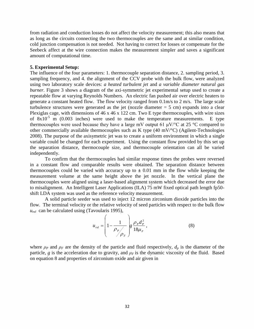
32

from radiation and conduction losses do not affect the velocity measurement; this also means that

as long as the circuits connecting the two thermocouples are the same and at similar condition,

cold junction compensation is not needed. Not having to correct for losses or compensate for the

Seebeck affect at the wire connection makes the measurement simpler and saves a significant

amount of computational time.

5. Experimental Setup:

The influence of the four parameters: 1. thermocouple separation distance, 2. sampling period, 3.

sampling frequency, and 4. the alignment of the CCV probe with the bulk flow, were analyzed

using two laboratory scale devices: a heated turbulent jet and a variable diameter natural gas

burner. Figure 3 shows a diagram of the axi-symmetric jet experimental setup used to create a

repeatable flow at varying Reynolds Numbers. An electric fan pushed air over electric heaters to

generate a constant heated flow. The flow velocity ranged from 0.1m/s to 2 m/s. The large scale

turbulence structures were generated as the jet (nozzle diameter = 5 cm) expands into a clear

Plexiglas cage, with dimensions of 46 x 46 x 122 cm. Two E type thermocouples, with wire sizes

of 8x10-5

m (0.003 inches) were used to make the temperature measurements. E type

thermocouples were used because they have a large mV output 61 μV/°C at 25 °C compared to

other commercially available thermocouples such as K type (40 mV/°C) (Agilent-Technologies

2008). The purpose of the axisymetric jet was to create a uniform environment in which a single

variable could be changed for each experiment. Using the constant flow provided by this set up

the separation distance, thermocouple size, and thermocouple orientation can all be varied

independently.

To confirm that the thermocouples had similar response times the probes were reversed

in a constant flow and comparable results were obtained. The separation distance between

thermocouples could be varied with accuracy up to ± 0.01 mm in the flow while keeping the

measurement volume at the same height above the jet nozzle. In the vertical plane the

thermocouples were aligned using a laser-based alignment system which decreased the error due

to misalignment. An Intelligent Laser Applications (ILA) 75 mW fixed optical path length fp50-

shift LDA system was used as the reference velocity measurement.

A solid particle seeder was used to inject 12 micron zirconium dioxide particles into the

flow. The terminal velocity or the relative velocity of seed particles with respect to the bulk flow

urel can be calculated using (Tavoularis 1995),

F

PP

F

P

rel

dgu

18

11

2

, (8)

where ρP and ρF are the density of the particle and fluid respectively, dp is the diameter of the

particle, g is the acceleration due to gravity, and μF is the dynamic viscosity of the fluid. Based

on equation 8 and properties of zirconium oxide and air given in

33

Table 3 the seed particles used in these experiments had a terminal velocity of 0.022 m/s. This is

accounted for in the results. A Honeywell Model 16200 hepa filter was used to remove the seed

particles from the flow after the jet passes out of the measurement volume.

In addition to an axi-symmetric jet, a natural gas burner was built to test the CCV probes

ability to work in a real fire scenario and analyse the ρxy decay above a fire as shown in figure 4.

The burner consists of a 1.22 m by 1.22 m square drywall top with the burner in the center. This

tabletop design kept the air entrainment horizontal at the fire base. The experimental apparatus

was constructed based on the classical study by Zukoski et al. 1980. The diameter of the burner

was adjusted by attaching a steel plate with a hole equal to the desired burner size. A schematic

of the burner geometry is shown as Figure 4. Natural gas was piped through a 2.54 cm stainless

steel braided tube into an air gap created by wire mesh, 5 cm of Kaowool and 10 cm of sand was

provide to ensure an even distribution of gas over the burner surface.

The purpose of testing over a burner was to test the viability of the CCV probe in a fire

induced buoyancy driven plume. Three thermocouples were used in the CCV probe so that the

separation distance did not have to be changed manually. The thermocouple separation distances

were adapted from the axi-symmetric jet experiments. They were set at 4 cm, and 8 cm providing

3 total separation distances (4, 8, and 12cm) with which to calculate the ρxy decay. The same E

type thermocouples used in the axi-symmetric jet were used here as-well. The thermocouples

were aligned in the vertical direction using a plumb bob before each test. Fires having base

diameters of 10 cm, 15 cm, and 20 cm and heat release rates between 6.2 kW to 23.7 kW were

tested. The heat release rate was determined by adjusting the flow of natural gas to the burner.

Measurements were taken at 4 heights above the plume (0.65m 0.98m, 1.22m, 1.54m). The

plume width was measured using a horizontal thermocouple tree using eight E type

thermocouples as shown in Figure 5. LDA measurements were not done in this scenario due to

seeding difficulties. Due to the low temperatures at the heights above the plume tested (

C 100~ ) radiation loss incurred a maximum of 0.8% error in the calculation of the plume

width and was not included.

6. Results and Analysis:

The results include velocities measured using the CCV technique and compared with

LDA measurements and characteristic turbulent length scales. Analysis of the influence of

sampling frequency, sampling time, and thermocouple alignment is also presented.

Figure 6 shows experimental results from varying the thermocouple separation distance

for Reynolds numbers between 300 and 6000. These Reynolds numbers correspond to a flow

velocity range between 0.1 m/s with a temperature ~2°C above ambient and 2.0 m/s with a

temperature ~20°C above ambient. The jet diameter was equal to 5 cm. The Reynolds number Re

was calculated using,

iud

Re , (9)

where u is the flow speed at the measurement volume, di is the nozzle diameter (5cm) of the jet

and ν is the kinematic viscosity of air. The measurements were taken 46 cm above the nozzle,

beyond the potential core which can extend 4-6 nozzle diameters (20-30 cm) into the jet (Kanury

1977). Each data point in Figure 6 represents the average of 12 consecutive measurements each

using a total sampling time tT = 15 s. The sampling frequency f = 10 kHz and thermocouple

separation distances: 5, 10, 20, 30, 40, 50, 60, and 70 mm were tested.

34

It was observed that the velocities measured by the CCV procedure and the LDA were

off by a factor of approximately 30%. This was consistent through the entire range of Reynolds

numbers tested. To account for this an experimental correction factor was included. The CCV

Reynolds numbers were corrected with a linear correction factor based solely on the measured

Reynolds number Rem using,

211ReRe aamc , (10)

where Rem is the measured Reynolds number using CCV and a1 and a2 are experimental

constants found to be 0.2301 and 188.16 respectively. This correction factor is partially due to

the terminal velocity of the seed particles, non-white noise4 in the data acquisition system, or a

non-axial component of the jet. At the lowest Reynolds numbers tested the terminal velocity

accounts for nearly the entire correction. At higher speeds it is believed that small

misalignments in the CCV probe with the flow angle play a larger role. Future work is needed to

analyse this correction factor. Using the correction factor discussed above, Figure 6 shows that

CCV measurement can generally report accuracies of within 5% of the LDA. The ability to

measure flows down to Re=300 (u=0.1m/s) is a significant advantage over current measuring

techniques such as the BDP. It was also found that the CCV technique is independent of

separation distance for values between 5 and 70 mm for the Reynolds numbers used in these

experiments. To study the effects of larger separation distances Figure 7 shows a plot of ρxy

verses d (10 mm to 120 mm). This figure shows a decay of the correlation coefficient as the

thermocouples become farther apart. If it is assumed that the decay is linear, extrapolation

shows that ρxy decays to 0.5 at a separation distance of 197mm. In the case of a circular free jet

the characteristic turbulent length scale is equal to the width of the jet and can be calculated

using (Kanury 1977),

ii d

xC

d241

2, (11)

where δ is the jet radius, di is the nozzle diameter (5 cm), x is the height above the nozzle (46

cm), and C is an empirical constant equal to 0.0128. Using equation 11 the width of the jet at the

measurement location was calculated as 191 mm, close to the 197 mm predicted by CCV.

To further analyse the use of the decay in ρxy to estimate the width of a flow, CCV

measurements with varying separation distances were taken along the centreline of the flow and

velocity measurements were taken with the LDA along the radius of the jet at different heights

above the nozzle. The edge of the jet was defined as a region when velocity decayed to 85% of

the maximum (velocity along centreline). Good agreement is observed between the two

methods. Figure 8 shows the length scales measured using LDA, and CCV. The dark solid line

is obtained using Kanuri’s correlation. Because Kanuri’s correlation predicts 100% of the jet

width, it was adjusted to 85% to match the LDA data. All CCV width measurements were below

the LDA measurements and Kanuri’s correlation predictions. The CCV measurement are less

than the reference measurements because any disturbance in the measurement will reduce the

nondimensional cross correlation coefficient and cause a smaller width calculation. These

disturbances include signal noise and misalignment with the plume angle with the thermocouple

probe.

Figure 8, shows that in addition to measurement of velocity and temperature at a given

location, CCV also allows estimation of the integral turbulent length scale, as previously defined,

4 Non-white noise is signal noise which is not distributed evenly across the spectrum of the signal.

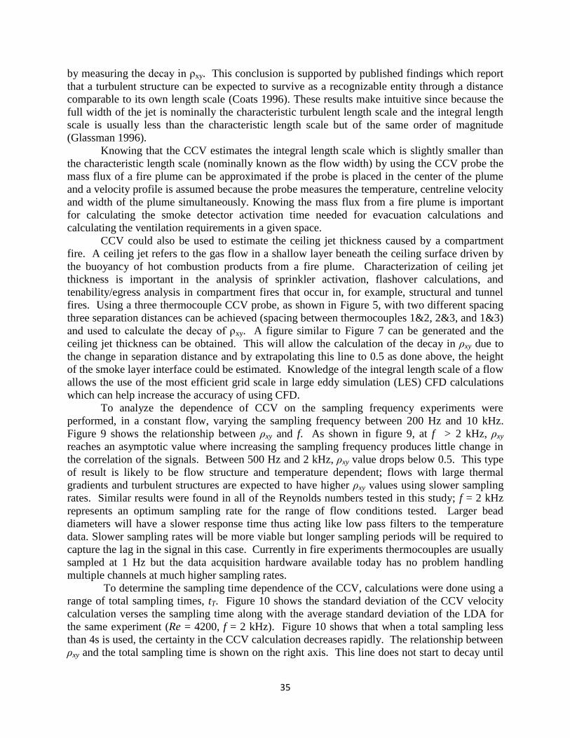
35

by measuring the decay in ρxy. This conclusion is supported by published findings which report

that a turbulent structure can be expected to survive as a recognizable entity through a distance

comparable to its own length scale (Coats 1996). These results make intuitive since because the

full width of the jet is nominally the characteristic turbulent length scale and the integral length

scale is usually less than the characteristic length scale but of the same order of magnitude

(Glassman 1996).

Knowing that the CCV estimates the integral length scale which is slightly smaller than

the characteristic length scale (nominally known as the flow width) by using the CCV probe the

mass flux of a fire plume can be approximated if the probe is placed in the center of the plume

and a velocity profile is assumed because the probe measures the temperature, centreline velocity

and width of the plume simultaneously. Knowing the mass flux from a fire plume is important

for calculating the smoke detector activation time needed for evacuation calculations and

calculating the ventilation requirements in a given space.

CCV could also be used to estimate the ceiling jet thickness caused by a compartment

fire. A ceiling jet refers to the gas flow in a shallow layer beneath the ceiling surface driven by

the buoyancy of hot combustion products from a fire plume. Characterization of ceiling jet

thickness is important in the analysis of sprinkler activation, flashover calculations, and

tenability/egress analysis in compartment fires that occur in, for example, structural and tunnel

fires. Using a three thermocouple CCV probe, as shown in Figure 5, with two different spacing

three separation distances can be achieved (spacing between thermocouples 1&2, 2&3, and 1&3)

and used to calculate the decay of ρxy. A figure similar to Figure 7 can be generated and the

ceiling jet thickness can be obtained. This will allow the calculation of the decay in ρxy due to

the change in separation distance and by extrapolating this line to 0.5 as done above, the height

of the smoke layer interface could be estimated. Knowledge of the integral length scale of a flow

allows the use of the most efficient grid scale in large eddy simulation (LES) CFD calculations

which can help increase the accuracy of using CFD.

To analyze the dependence of CCV on the sampling frequency experiments were

performed, in a constant flow, varying the sampling frequency between 200 Hz and 10 kHz.

Figure 9 shows the relationship between ρxy and f. As shown in figure 9, at f > 2 kHz, ρxy

reaches an asymptotic value where increasing the sampling frequency produces little change in

the correlation of the signals. Between 500 Hz and 2 kHz, ρxy value drops below 0.5. This type

of result is likely to be flow structure and temperature dependent; flows with large thermal

gradients and turbulent structures are expected to have higher ρxy values using slower sampling

rates. Similar results were found in all of the Reynolds numbers tested in this study; f = 2 kHz

represents an optimum sampling rate for the range of flow conditions tested. Larger bead

diameters will have a slower response time thus acting like low pass filters to the temperature

data. Slower sampling rates will be more viable but longer sampling periods will be required to

capture the lag in the signal in this case. Currently in fire experiments thermocouples are usually

sampled at 1 Hz but the data acquisition hardware available today has no problem handling

multiple channels at much higher sampling rates.

To determine the sampling time dependence of the CCV, calculations were done using a

range of total sampling times, tT. Figure 10 shows the standard deviation of the CCV velocity

calculation verses the sampling time along with the average standard deviation of the LDA for

the same experiment (Re = 4200, f = 2 kHz). Figure 10 shows that when a total sampling less

than 4s is used, the certainty in the CCV calculation decreases rapidly. The relationship between

ρxy and the total sampling time is shown on the right axis. This line does not start to decay until

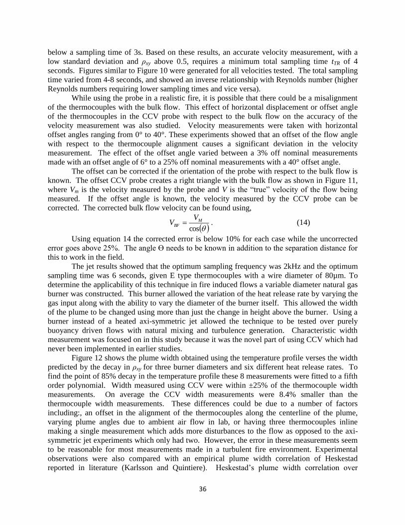
36

below a sampling time of 3s. Based on these results, an accurate velocity measurement, with a

low standard deviation and ρxy above 0.5, requires a minimum total sampling time tTR of 4

seconds. Figures similar to Figure 10 were generated for all velocities tested. The total sampling

time varied from 4-8 seconds, and showed an inverse relationship with Reynolds number (higher

Reynolds numbers requiring lower sampling times and vice versa).

While using the probe in a realistic fire, it is possible that there could be a misalignment

of the thermocouples with the bulk flow. This effect of horizontal displacement or offset angle

of the thermocouples in the CCV probe with respect to the bulk flow on the accuracy of the

velocity measurement was also studied. Velocity measurements were taken with horizontal

offset angles ranging from 0° to 40°. These experiments showed that an offset of the flow angle

with respect to the thermocouple alignment causes a significant deviation in the velocity

measurement. The effect of the offset angle varied between a 3% off nominal measurements

made with an offset angle of 6° to a 25% off nominal measurements with a 40° offset angle.

The offset can be corrected if the orientation of the probe with respect to the bulk flow is

known. The offset CCV probe creates a right triangle with the bulk flow as shown in Figure 11,

where Vm is the velocity measured by the probe and V is the “true” velocity of the flow being

measured. If the offset angle is known, the velocity measured by the CCV probe can be

corrected. The corrected bulk flow velocity can be found using,

cos

MBF

VV . (14)

Using equation 14 the corrected error is below 10% for each case while the uncorrected

error goes above 25%. The angle Ө needs to be known in addition to the separation distance for

this to work in the field.

The jet results showed that the optimum sampling frequency was 2kHz and the optimum

sampling time was 6 seconds, given E type thermocouples with a wire diameter of 80µm. To

determine the applicability of this technique in fire induced flows a variable diameter natural gas

burner was constructed. This burner allowed the variation of the heat release rate by varying the

gas input along with the ability to vary the diameter of the burner itself. This allowed the width

of the plume to be changed using more than just the change in height above the burner. Using a

burner instead of a heated axi-symmetric jet allowed the technique to be tested over purely

buoyancy driven flows with natural mixing and turbulence generation. Characteristic width

measurement was focused on in this study because it was the novel part of using CCV which had

never been implemented in earlier studies.

Figure 12 shows the plume width obtained using the temperature profile verses the width

predicted by the decay in ρxy for three burner diameters and six different heat release rates. To

find the point of 85% decay in the temperature profile these 8 measurements were fitted to a fifth

order polynomial. Width measured using CCV were within ±25% of the thermocouple width

measurements. On average the CCV width measurements were 8.4% smaller than the

thermocouple width measurements. These differences could be due to a number of factors

including:, an offset in the alignment of the thermocouples along the centerline of the plume,

varying plume angles due to ambient air flow in lab, or having three thermocouples inline

making a single measurement which adds more disturbances to the flow as opposed to the axi-

symmetric jet experiments which only had two. However, the error in these measurements seem

to be reasonable for most measurements made in a turbulent fire environment. Experimental

observations were also compared with an empirical plume width correlation of Heskestad

reported in literature (Karlsson and Quintiere). Heskestad’s plume width correlation over

37

predicts experimental results by 25%. This is mainly due to the small fire sizes used in this

study.

7. Conclusions:

This study examines four factors affecting the CCV measurement. These are the

thermocouple separation distance, the sampling period, the sampling frequency, and angular

alignment dependence of the technique. Two experimental set ups, a turbulent jet and a natural

gas burner were designed to analyze the four factors. It was found that thermocouple separation

distance had little effect on the accuracy of the velocity measurement as long as the separation

distance is smaller than the characteristic turbulent length scale. However, separation distance

has a large effect on the cross correlation, ρxy of the signal between two thermocouples. Based

on the standard deviation of the velocity measurements and the value of ρxy the optimum

sampling frequency for the range of Reynolds numbers tested is 2 kHz. Above this value the

strength in the correlation coefficient does not change significantly and below this value ρxy

begins to decay. The minimum required sampling time was found to vary between 4 and 8

seconds.

It was shown that the error due to misalignment of the CCV probe with the bulk flow

direction could be corrected if the angle is known. The nondimensional cross correlation

coefficient decreased in a linear fashion as the thermocouple separation distance is increased.

This linear decay can be used to estimate the integral turbulent length scale of the turbulent

flows. Experiments with the natural gas burner showed that a CCV probe can measure

temperature, velocity, and plume width simultaneously which allows the calculation of an

estimation of the total mass flux of a fire plume, optimize CFD grid sizing, and ceiling jet

thicknesses in a developing compartment fire.

8. Acknowledgements:

The authors would like to thank the Society of Fire Protection Engineering, and the National

Science Foundation Graduate Research Fellowship Program for helping to fund this research.

The help of laboratory manager Randy Harris is also acknowledged.

9. Figures and Tables:

Table 2: Velocity measurement methods widely in use

* technique proposed in this study

Device Operating Principle Cost Accuracy

Bi-directional probe (BDP) ∆P ~$1000 <10 %

Pitot tube ∆P <10 %

Hot wire anemometer (HWA) ∆T ~$1000 <25 %

Laser Doppler Anemometer (LDA) Scattered Shifted Laser Light ~$80,000 <4 %

Particle Image Velocimetry (PIV) Scattered Laser Light ~100,000 <5 %

Cross Correlation Velocimetry (CCV)* Temperature Fluctuations ~$100 <5 %

5 Dependent on flow temperature and temperature fluctuations.

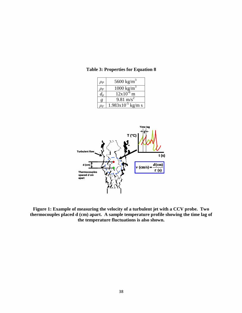
38

Table 3: Properties for Equation 8

ρP 5600 kg/m3

ρF 1000 kg/m3

dp 12x10-6

m

g 9.81 m/s2

μF 1.983x10-5

kg/m s

Figure 1: Example of measuring the velocity of a turbulent jet with a CCV probe. Two

thermocouples placed d (cm) apart. A sample temperature profile showing the time lag of

the temperature fluctuations is also shown.

Turbulent flow

T (°C)

t (s)

Time lag

(cm) (cm/s)

(s)

dv

d (cm)

Thermocouples

spaced d cm

apart

Turbulent flow

T (°C)

t (s)

Time lag

(cm) (cm/s)

(s)

dv

d (cm)

Thermocouples

spaced d cm

apart

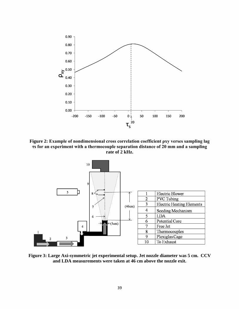
39

Figure 2: Example of nondimensional cross correlation coefficient ρxy verses sampling lag

τs for an experiment with a thermocouple separation distance of 20 mm and a sampling

rate of 2 kHz.

Figure 3: Large Axi-symmetric jet experimental setup. Jet nozzle diameter was 5 cm. CCV

and LDA measurements were taken at 46 cm above the nozzle exit.

40

Figure 4: Natural gas burner base with drywall tabletop. Floor dimensions were 1.22 m

square on top with the table top 0.6m off the floor.

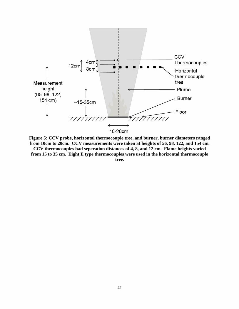
41

Figure 5: CCV probe, horizontal thermocouple tree, and burner, burner diameters ranged

from 10cm to 20cm. CCV measurements were taken at heights of 56, 98, 122, and 154 cm.

CCV thermocouples had seperation distances of 4, 8, and 12 cm. Flame heights varied

from 15 to 35 cm. Eight E type thermocouples were used in the horizontal thermocouple

tree.

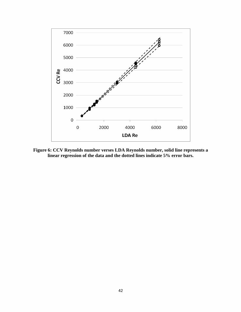
42

Figure 6: CCV Reynolds number verses LDA Reynolds number, solid line represents a

linear regression of the data and the dotted lines indicate 5% error bars.

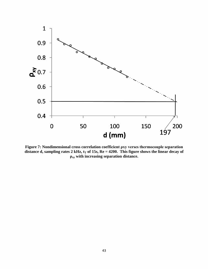
43

Figure 7: Nondimensional cross correlation coefficient ρxy verses thermocouple separation

distance d, sampling rates 2 kHz, tT of 15s, Re = 4200. This figure shows the linear decay of

ρxy with increasing separation distance.

44

Figure 8: Diameter of turbulent free jet verses height above nozzle.

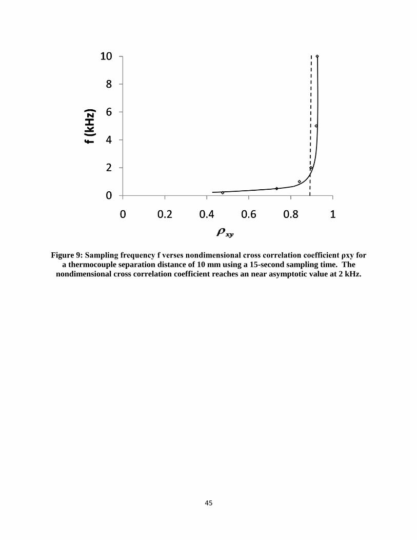
45

Figure 9: Sampling frequency f verses nondimensional cross correlation coefficient ρxy for

a thermocouple separation distance of 10 mm using a 15-second sampling time. The

nondimensional cross correlation coefficient reaches an near asymptotic value at 2 kHz.

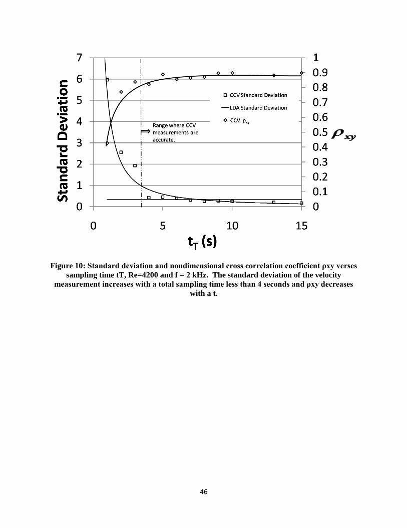
46

Figure 10: Standard deviation and nondimensional cross correlation coefficient ρxy verses

sampling time tT, Re=4200 and f = 2 kHz. The standard deviation of the velocity

measurement increases with a total sampling time less than 4 seconds and ρxy decreases

with a t.

47

Figure 11: Right triangle created by CCV thermocouples and bulk flow velocity.

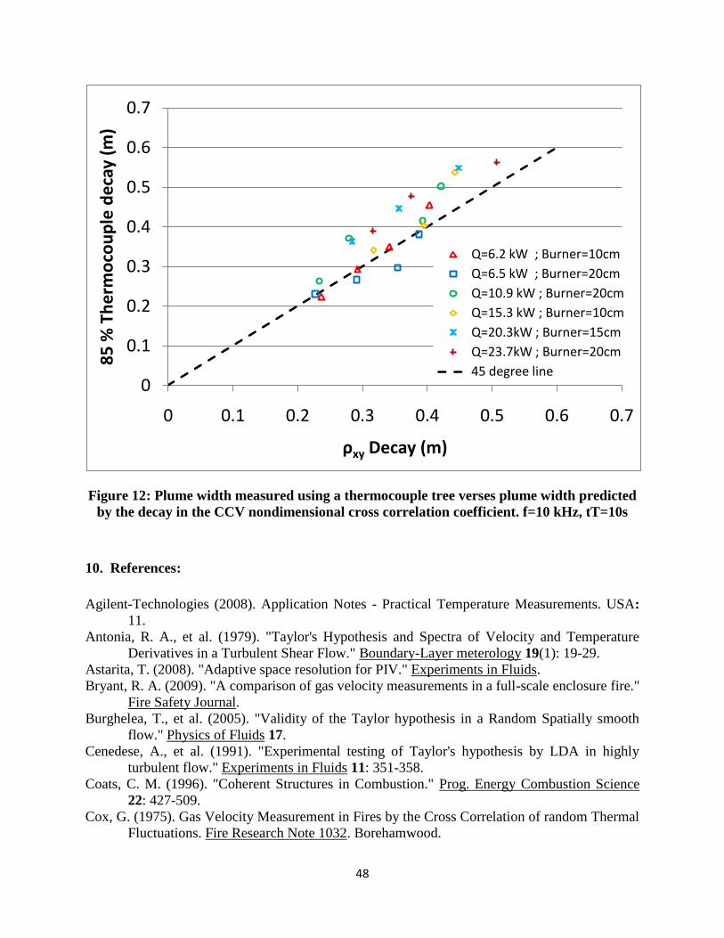
48

Figure 12: Plume width measured using a thermocouple tree verses plume width predicted

by the decay in the CCV nondimensional cross correlation coefficient. f=10 kHz, tT=10s

10. References:

Agilent-Technologies (2008). Application Notes - Practical Temperature Measurements. USA:

11.

Antonia, R. A., et al. (1979). "Taylor's Hypothesis and Spectra of Velocity and Temperature

Derivatives in a Turbulent Shear Flow." Boundary-Layer meterology 19(1): 19-29.

Astarita, T. (2008). "Adaptive space resolution for PIV." Experiments in Fluids.

Bryant, R. A. (2009). "A comparison of gas velocity measurements in a full-scale enclosure fire."

Fire Safety Journal.

Burghelea, T., et al. (2005). "Validity of the Taylor hypothesis in a Random Spatially smooth

flow." Physics of Fluids 17.

Cenedese, A., et al. (1991). "Experimental testing of Taylor's hypothesis by LDA in highly

turbulent flow." Experiments in Fluids 11: 351-358.

Coats, C. M. (1996). "Coherent Structures in Combustion." Prog. Energy Combustion Science

22: 427-509.

Cox, G. (1975). Gas Velocity Measurement in Fires by the Cross Correlation of random Thermal

Fluctuations. Fire Research Note 1032. Borehamwood.

0

0.1

0.2

0.3

0.4

0.5

0.6

0.7

0 0.1 0.2 0.3 0.4 0.5 0.6 0.7

85

% T

he

rmo

cou

ple

de

cay

(m)

ρxy Decay (m)

Q=6.2 kW ; Burner=10cm

Q=6.5 kW ; Burner=20cm

Q=10.9 kW ; Burner=20cm

Q=15.3 kW ; Burner=10cm

Q=20.3kW ; Burner=15cm

Q=23.7kW ; Burner=20cm

45 degree line

49

Cox, G. (1976). "Some Measurements of Fire Turbulence." Fire and Mat. 1: 116-122.

Cox, G. (1977). "Gas Velocity Measurements in Fires by the Cros-Correlation of Random

Thermal Fluctuations- A Comparison with Conventional Techniques." Comb. and Flame

28: 155-163.

Cox, G. and R. Chitty (1980). "Study of the Deterministic Properties of Unbounded Fire

Plumes." Comb. and Flame 39: 191-209.

Degraaff, D. B. and J. K. Eaton (2001). "A high-resolution laser Doppler anemometer: design,

qualification, and uncertainty." Experiments in Fluids 30: 522-530.

Drysdale, D. (1999). An Introduction to Fire Dynamics, John Wiley & Sons.

Dupuy, J. L., et al. (1998). "Measurement of temperatures and radiant heat fluxes during static

fires in a porous fuel." Proceedings of 3rd international conference on forest fire

research–14th conference on fire and forest meteorology: 16–20.

Dupuy, J. L., et al. (2003). "Fires from a Cylindrical Forest Fuel Burner: Combustion Dynamics

and Flame Properties." Comb. and Flame 135(1-2): 65-76.

Favre, A. J., et al. (2006). "Space-time double correlations and spectra in a turbulent boundary

layer." Journal of Fluid Mechanics Digital Archive 2(04): 313-342.

Favre, H. (1948). "The influence of its own weight on the stability of a rectangular plate." Proc.,

7th Int. Congress of Applied Mechanics, Organising Committee, London 1: 151–159.

Glassman, I. (1996). Combustion, Academic Press San Diego, Calif.

Grosshandler, W. (2000). Measurement Needs for Fire Safety. NISTIR 6527.

Kanury, A. M. (1977). An Introduction to Combustion Phenomena, Gordon & Breach Science

Publishers, Inc.

Karlsson, B. and J. G. Quintiere (2000). Enclosure Fire Dynamics, CRC Press.

Koslowski, C. C. (1991). Effects of Beams and Ceiling Obstructions on Steady State Ceiling Jet

Flow. Fire Protection Engineering. Worcester, Worcester Polytechnic Institute. MS.

Kundu, P. K. and I. M. Cohen (1987). Fluid Mechanics, Academic press.

Marcelli, T., et al. (2004). "Fire Spread Across Pine Needle Fuel Beds: Characterization of

Temperature and Velocity Distributions Within the Fire Plume." International Journal of

Wildland Fire 13: 37-48.

Marrion, C. (1989). Lag Time Modeling and Effects of Ceiling Jet Velocity on The Placement of

Optical Smoke Detectors. Fire Protection Engineering. Worcester, Worcester Polytechnic

Institute. Masters of Science 211.

Marvasti, M. A. and W. C. Strahle (1994). "Fractal interpolation methods in spatial cross-

correlation velocimetry." Experiments in Fluids 18: 129-130.

McCaffrey, B. and G. Heskestad (1976). "A Robust Bidirectional Low-Velocity Probe for Flame

and Fire Application." Comb. and Flame 26(1): 125-127.

Morgan, M. G. and K. L. Bowles (1968). "Cross-Correlation and Cross-Spectral Methods for

Drift Velocity Measurements." Science 161(3846): 1139-1142.

Motevalli, V. (1989). A Study of the Characteristics of Small-Scale Unconfined Fire Induced

Ceiling Jets. ME, University of Maryland, College Park. Ph.D.

Motevalli, V., et al. (1992). "Cross-correlation velocimetry for measurement of velocity and

temperature profiles in low-speed, turbulent, nonisothermal flows." Journal of Heat

Transfer (Transactions of the ASME).

Santoni, P. A., et al. (2002). "Measurement of Fluctuating Temperatures in a Continuous Flame

Spreading across a Fuel bed using a Double Thermocouple Probe." Comb. and Flame

131(1): 47-58.

50

Sette, B. J. G. (2006). "Development of a Velocity Pressure Probe." Fire and Mat. 30: 397-414.

Tagawa, M., et al. (2003). "Response compensation of thermistors: Frequency response and

identification of thermal time constant." Review of Scientific Instruments 74: 1350.

Tagawa, M. and Y. Ohta (1997). "Two-Thermocouple Probe for Fluctuating Temperature

Measurement in Combustion--Rational Estimation of Mean and Fluctuating Time

Constants." Combust. Flame 109(4): 549-560.

Tavoularis, S. (1995). Measurement in Fluid Mechanics. Cambridge, Cambridge University

Press.

Taylor, G. I. (1938). "The Spectrum of Turbulence." Proc Roy. Soc. A 164: 476-490.

Tennekes, H. and J. L. Lumley (1972). A First Course in Turbulence. Cambridge, MA, The MIT

Press.

Tieszen, S. R. (2001). "On the Fluid Mechanics of Fires." Annual Rev. Fluid Mech. 33: 67-92.

Torero, J. L. and R. Carvel (2007). The Dalmarnock fire Tests: Experiments and Modeling,

School of Engineering and Electronics, University of Edinburgh.

Turns, S. R. (2000). An Introduction to Combustion: Concepts and Applications. New York,

McGraw Hill.

Wills, J. A. B. (1964). "On Convection Velocities in turbulent Shear Flows." Journal of Fluid

Mechanics 20(3): 417-432.

Young, C. N. (1998). Thermocouple Compensation. Mechanical Engineering. Waterloo, Ontario.

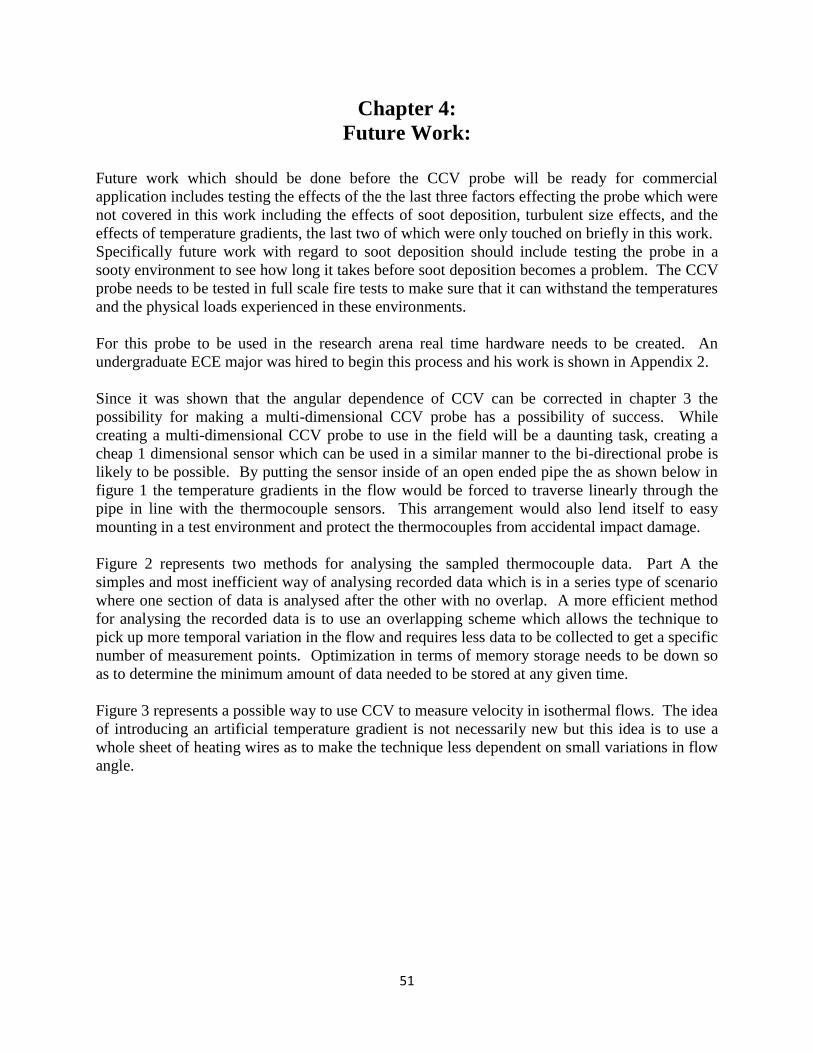
51

Chapter 4:

Future Work:

Future work which should be done before the CCV probe will be ready for commercial

application includes testing the effects of the the last three factors effecting the probe which were

not covered in this work including the effects of soot deposition, turbulent size effects, and the

effects of temperature gradients, the last two of which were only touched on briefly in this work.

Specifically future work with regard to soot deposition should include testing the probe in a

sooty environment to see how long it takes before soot deposition becomes a problem. The CCV

probe needs to be tested in full scale fire tests to make sure that it can withstand the temperatures

and the physical loads experienced in these environments.

For this probe to be used in the research arena real time hardware needs to be created. An

undergraduate ECE major was hired to begin this process and his work is shown in Appendix 2.

Since it was shown that the angular dependence of CCV can be corrected in chapter 3 the

possibility for making a multi-dimensional CCV probe has a possibility of success. While

creating a multi-dimensional CCV probe to use in the field will be a daunting task, creating a

cheap 1 dimensional sensor which can be used in a similar manner to the bi-directional probe is

likely to be possible. By putting the sensor inside of an open ended pipe the as shown below in

figure 1 the temperature gradients in the flow would be forced to traverse linearly through the

pipe in line with the thermocouple sensors. This arrangement would also lend itself to easy

mounting in a test environment and protect the thermocouples from accidental impact damage.

Figure 2 represents two methods for analysing the sampled thermocouple data. Part A the

simples and most inefficient way of analysing recorded data which is in a series type of scenario

where one section of data is analysed after the other with no overlap. A more efficient method

for analysing the recorded data is to use an overlapping scheme which allows the technique to

pick up more temporal variation in the flow and requires less data to be collected to get a specific

number of measurement points. Optimization in terms of memory storage needs to be down so

as to determine the minimum amount of data needed to be stored at any given time.

Figure 3 represents a possible way to use CCV to measure velocity in isothermal flows. The idea

of introducing an artificial temperature gradient is not necessarily new but this idea is to use a

whole sheet of heating wires as to make the technique less dependent on small variations in flow

angle.

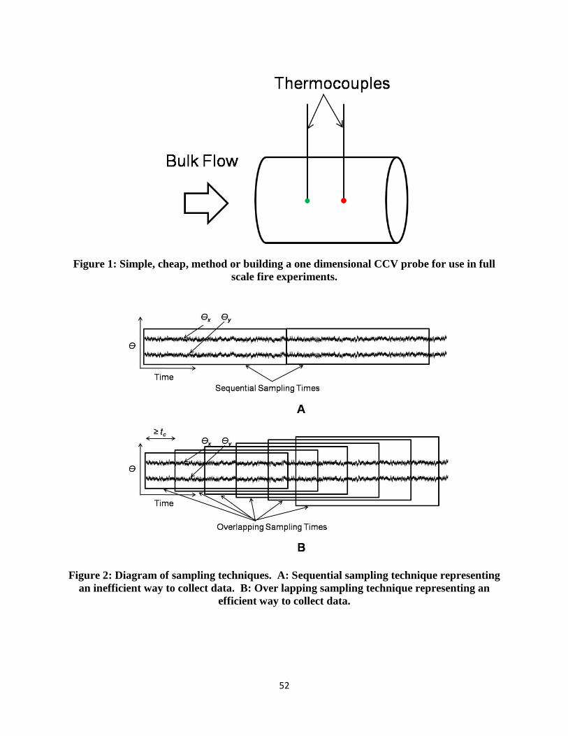
52

Figure 1: Simple, cheap, method or building a one dimensional CCV probe for use in full

scale fire experiments.

Figure 2: Diagram of sampling techniques. A: Sequential sampling technique representing

an inefficient way to collect data. B: Over lapping sampling technique representing an

efficient way to collect data.

53

Figure 3: Possible way to use a heated wire to generate artificial heat waves with which to

measure velocity in an iso-thermal flow.

54

Appendix 1: MATLAB script to Cross correlate thermocouple

signals and generate velocity results.

%% Written by Scott Rockwell

% 12/13/08

% last modified 05/01/09

%% Basics

clc

; % Clear command window

clear all

; % Clear Workspace

close all

; % Close open figures

tic

; % Start recording cpu time

dname = ('C:\Documents and

Settings\srockwel\My Documents\2 WPI research\Axi-symetric jet\Test

Data\Field Exp\Calibration test');%Default Directory To be Opened

dt = 10

;

num_data_pts = 1810000

; % Tells the crossCorr_fxn how many data points to use incase I wran two

tests back to back = hz rate times (run time+1)

%% Set up basic file name path to read

top_file = [dname '\']

; %Set up main database to open and look inside

ls_top_file = ls(top_file)

; %List Files inside main folder

c = cellstr(ls_top_file)

; %Turn cells from ls function into strings

cc = c(3:length(c))

; %Set up a matrix without the . and .. produces by the ls function

S = size(cc)

; %Find the size of matrix containing names of files inside of main

database

a = 1

; %This counter is set to 3 to account for the . and .. at the begining of

each matrix created by the ls function, the need for this was eliminated in

the two nested loops

count1 = 1

;

count2 = 1

;

while a <= S(1)

file = char(cellstr([top_file

char(cc(a))])) ; %File to be operated on

data_n = char(cc(a))

file_name = char(cc(a))

;

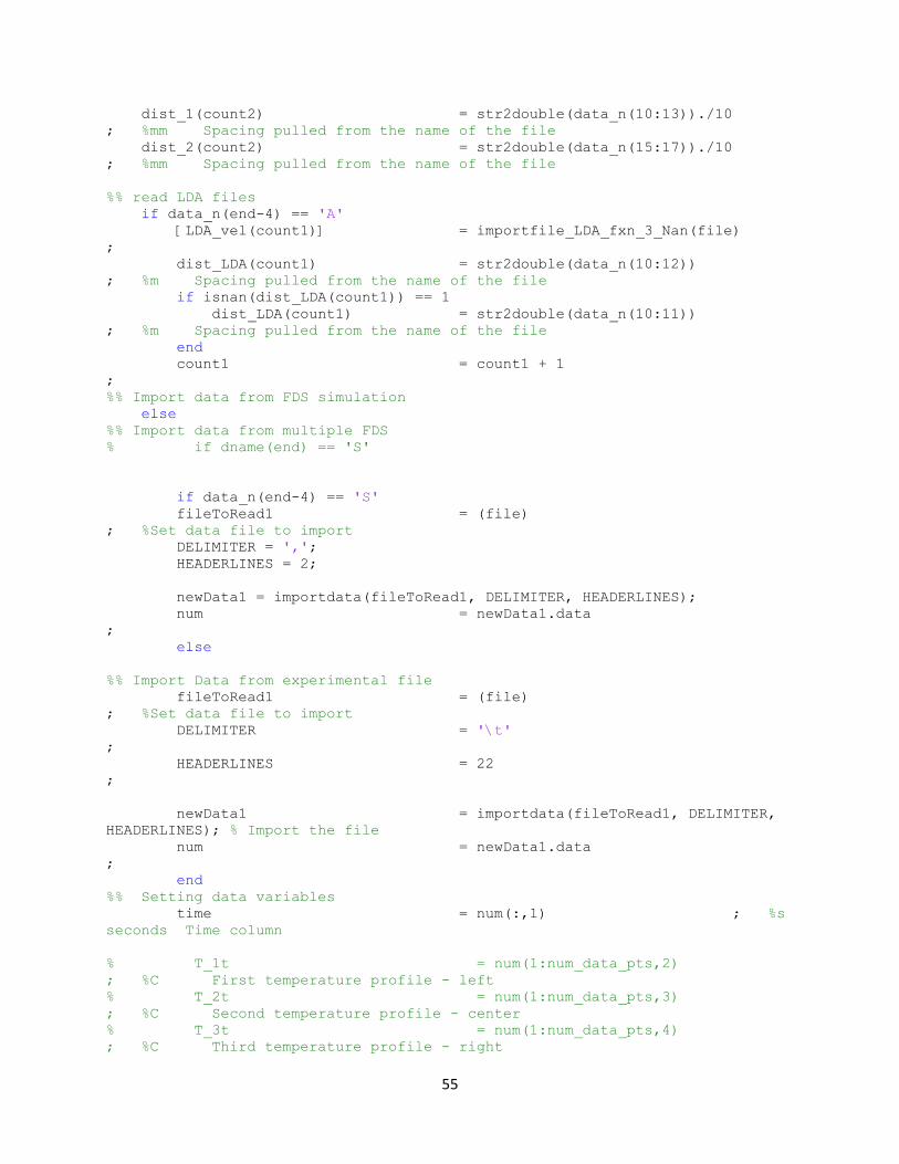
55

dist_1(count2) = str2double(data_n(10:13))./10

; %mm Spacing pulled from the name of the file

dist_2(count2) = str2double(data_n(15:17))./10

; %mm Spacing pulled from the name of the file

%% read LDA files

if data_n(end-4) == 'A'

[LDA_vel(count1)] = importfile_LDA_fxn_3_Nan(file)

;

dist_LDA(count1) = str2double(data_n(10:12))

; %m Spacing pulled from the name of the file

if isnan(dist_LDA(count1)) == 1

dist_LDA(count1) = str2double(data_n(10:11))

; %m Spacing pulled from the name of the file

end

count1 = count1 + 1

;

%% Import data from FDS simulation

else

%% Import data from multiple FDS

% if dname(end) == 'S'

if data_n(end-4) == 'S'

fileToRead1 = (file)

; %Set data file to import

DELIMITER = ',';

HEADERLINES = 2;

newData1 = importdata(fileToRead1, DELIMITER, HEADERLINES);

num = newData1.data

;

else

%% Import Data from experimental file

fileToRead1 = (file)

; %Set data file to import

DELIMITER = '\t'

;

HEADERLINES = 22

;

newData1 = importdata(fileToRead1, DELIMITER,

HEADERLINES); % Import the file

num = newData1.data

;

end

%% Setting data variables

time = num(:,1) ; %s

seconds Time column

% T_1t = num(1:num_data_pts,2)

; %C First temperature profile - left

% T_2t = num(1:num_data_pts,3)

; %C Second temperature profile - center

% T_3t = num(1:num_data_pts,4)

; %C Third temperature profile - right

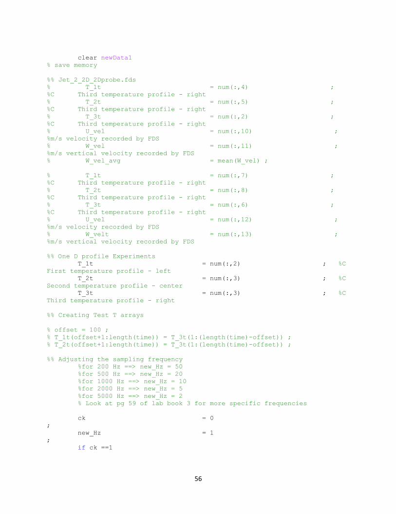
56

clear newData1

% save memory

%% Jet_2_2D_2Dprobe.fds

% T_1t = num(:,4) ;

%C Third temperature profile - right

% T_2t = num(:,5) ;

%C Third temperature profile - right

% T_3t = num(:,2) ;

%C Third temperature profile - right

% U_vel = num(:,10) ;

%m/s velocity recorded by FDS

% W_vel = num(:,11) ;

%m/s vertical velocity recorded by FDS

% W_vel_avg = mean(W_vel) ;

% T_1t = num(:,7) ;

%C Third temperature profile - right

% T_2t = num(:,8) ;

%C Third temperature profile - right

% T_3t = num(:,6) ;

%C Third temperature profile - right

% U_vel = num(:,12) ;

%m/s velocity recorded by FDS

% W_velt = num(:,13) ;

%m/s vertical velocity recorded by FDS

%% One D profile Experiments

T_1t = num(:,2) ; %C

First temperature profile - left

T_2t = num(:,3) ; %C

Second temperature profile - center

T_3t = num(:,3) ; %C

Third temperature profile - right

%% Creating Test T arrays

% offset = 100 ;

% T_1t(offset+1:length(time)) = T_3t(1:(length(time)-offset)) ;

% T_2t(offset+1:length(time)) = T_3t(1:(length(time)-offset)) ;

%% Adjusting the sampling frequency

%for 200 Hz ==> new_Hz = 50

%for 500 Hz ==> new_Hz = 20

%for 1000 Hz ==> new_Hz = 10

%for 2000 Hz ==> new_Hz = 5

%for 5000 Hz ==> new_Hz = 2

% Look at pg 59 of lab book 3 for more specific frequencies

ck = 0

;

new_Hz = 1

;

if ck ==1

57

new_length = length(time)/new_Hz

;

time_temp = zeros(1,new_length)

;

T_1t_temp = zeros(1,new_length)

;

T_2t_temp = zeros(1,new_length)

;

T_3t_temp = zeros(1,new_length)

;

ct_1 = 1

;

for dd = 1:new_Hz:length(time)

;

time_temp(ct_1) = time(dd)

;

T_1t_temp(ct_1) = T_1t(dd)

;

T_2t_temp(ct_1) = T_2t(dd)

;

T_3t_temp(ct_1) = T_3t(dd)

;

ct_1 = ct_1+1

;

end

clear time T_1t T_2t T_3t

time = time_temp

;

T_1t = T_1t_temp

;

T_2t = T_2t_temp

;

T_3t = T_3t_temp

;

end

if data_n(end-4) == 'S'

del_t = zeros (1, length(time)-1) ;

for ct_3 = 1:length(time)-1

del_t(ct_3) = time(ct_3+1)-time(ct_3) ;

end

del_t_avg = mean(del_t) ;

Hz = round(1/(del_t_avg))

; %Hz Sampling rate

check = 1 ;

else

Hz = round(1/(time(2)-time(1))) ; %Hz

Sampling rate

end

%% Break the time step into sections based on the specified dt split time

split = dt*Hz

;

over_lap = round(split/1) ; % Number of data

points between calculation matrix

%if over_lap = split ==> sequential calculation

%if over_lap < split ==> some type of overlapping calculation

58

tt = 1

;

T_1ss = zeros(round((length(T_1t)-split)./over_lap), split+1) ;

T_2ss = zeros(round((length(T_1t)-split)./over_lap), split+1) ;

T_3ss = zeros(round((length(T_1t)-split)./over_lap), split+1) ;

for t = 1:over_lap:length(T_1t)-split

% Splitting temperature profile into sections

T_1ss(tt,:) = T_1t(t:t+split)

;

T_2ss(tt,:) = T_2t(t:t+split)

;

T_3ss(tt,:) = T_3t(t:t+split)

;

tt = tt+1

;

end

%% Start Calculation Loop

S_T_1ss = size(T_1ss)

;

for ss = 1:1:S_T_1ss(1)

T_1 = T_1ss(ss,:)

; % Setting temperature profiles to be calculated

T_2 = T_2ss(ss,:)

; % " "

T_3 = T_3ss(ss,:)

; % " "

maxlag = 2500/new_Hz

; % maximum size of sampling lag

window_size = length(T_1)-2*(maxlag+1)

; % length of data profile to use

T_1s = T_1(maxlag+1:maxlag+window_size)

; % create 1st correlated profile

T_1s = T_1s - mean(T_1)

; % Normalizing the temperature profile

T_2s = T_2(maxlag+1:maxlag+window_size)

; % create 1st correlated profile

T_2s = T_2s - mean(T_2)

; % Normalizing the temperature profile

sigma_13 = std(T_1)*std(T_3)

; % Calculating standard deviation

sigma_23 = std(T_2)*std(T_3)

; % Calculating standard deviation

CCC1 = zeros(2*maxlag+1,1)

; % create initial CC coefficient matrix

CCC2 = zeros(2*maxlag+1,1)

; % create initial CC coefficient matrix

%% Cross Correlation claculations

for i = -maxlag:maxlag

T_3s =

T_3(i+maxlag+1:i+maxlag+window_size) ;

59

T_3s_avg = mean(T_3s) ;

T_3_avg = mean(T_3) ;

T_3s = T_3s - mean(T_3)

;

% sigma_13 = std(T_1s)*std(T_3s)

; % Calculating standard deviation

% sigma_23 = std(T_2s)*std(T_3s)

; % Calculating standard deviation

%

CCC1(i+maxlag+1) =

(T_3s*T_1s')/(length(T_3s)*sigma_13) ; % Cross correlation 1st side

CCC2(i+maxlag+1) =

(T_3s*T_2s')/(length(T_3s)*sigma_23) ; % Cross correlation 2nd side

end

% lag_spacing = (1:2*maxlag+1) - (maxlag+1)

; % Create matrix is lag spacings

lag_spacing = (1:2*maxlag+1) - (maxlag+1)

; % Create matrix is lag spacings

%% Setting 0 lag to zero

lag_0 = find(lag_spacing==0) ;

% Find position of lag spacing of zero in lag matrix

CCC1(lag_0) = 0 ; % Set

lag of zero = 0

CCC2(lag_0) = 0 ; % Set

lag of zero = 0

%% Plot Comparison

close all

figure

hold on

plot(lag_spacing, CCC1)

plot(lag_spacing, CCC2,'r')

hold off

pause(0.2)

% break

%%

%% End Copy code

CCC1s = CCC1 ;

CCC2s = CCC2 ;

%% Setting 0 lag to average of points around it - two points out

% lag_0 = find(lag_spacing==0)

; % Find position of lag spacing of zero in lag matrix

% CCC1(lag_0-2:lag_0+2) = (CCC1(lag_0-2)+CCC1(lag_0+2))./2

+1e-5 ; %

% CCC2(lag_0-2:lag_0+2) = (CCC2(lag_0-2)+CCC2(lag_0+2))./2

+1e-5 ; %

60

%% Simple Low Pass Filter

% CCC_N1 = zeros(2*maxlag+1,1)

;

% CCC_N2 = zeros(2*maxlag+1,1)

;

% num_pt_ave = 5

; % number of points being averaged

% for ii = num_pt_ave+1:length(CCC1)-(num_pt_ave+1)

% CCC_N1(ii) = mean( CCC1(ii-num_pt_ave :

ii+num_pt_ave ) );

% CCC_N2(ii) = mean( CCC2(ii-num_pt_ave :

ii+num_pt_ave ) );

% end

%

% clear CCC1 CCC2

% CCC1 = CCC_N1

;

% CCC2 = CCC_N2

;

%% Plotting Nondimensional cross correlation coefficient

% close all

% figure

% hold on

% plot(lag_spacing,CCC1s,'k')

% plot(lag_spacing,CCC2s,'r')

% axis([-maxlag maxlag 0 1])

% % axis([-20 20 0.7 1])

% grid on

% pause(0.2)

% hold off

%% Note

% When going to 3D make look crating matrix of CCC's using ct_1 so each one

will be ccc(ct_1) instead of CCC1, CCC2, CCC3

%% Calculating Peaks

m_CC1 = max(CCC1)

; % Find max CC coefficient

peak_pos1 = find(CCC1 == m_CC1 )

; % Find position of max CC coefficient (peak)

m_CC2 = max(CCC2)

; % Find max CC coefficient

peak_pos2 = find(CCC2 == m_CC2 )

; % Find position of max CC coefficient (peak)

lag1(ss, count2) = lag_spacing(peak_pos1(1))

; % supposidly the offset

lag2(ss, count2) = lag_spacing(peak_pos2(1))

; % supposidly the offset

%% Do trig to find vector

theta(ss, count2) = atan(lag1(ss, count2)/lag2(ss,

count2)) ; % Angle of flow vector

61

theta_degree(ss, count2) = theta(ss, count2)*180./pi()

; % angle of flow in degrees

% lag_correct(ss, count2) = lag1(ss, count2)*cos(theta(ss,

count2)) ; % corrected lag based on angle

% TC_vel_correct(ss,count2) =

(dist_1(count2)./1000)./(lag_correct(ss,count2))*Hz ; %m/s Velocity from

Termocouple measurements

% Averaging individual lags together to find velocity

lag1_avg(ss, count2) = mean(lag1(1:ss,count2))

; % average of lag 1

lag2_avg(ss, count2) = mean(lag2(1:ss,count2))

; % average of lag 2

%

% theta_avg(ss, count2) = atan(lag1_avg(ss,

count2)/lag2_avg(ss, count2)) ; % Angle of flow vector

% theta_degree_avg(ss, count2)= theta_avg(ss, count2)*180./pi()

; % angle of flow in degrees

rho_1(ss, count2) = m_CC1

; % Save non-dimensionalized coefficient ;

rho_2(ss, count2) = m_CC2

; % Save non-dimensionalized coefficient ;

end

%% Calculate velocities and angles

TC_vel_1(:,count2) =

(dist_1(count2)./1000)./(lag1(:,count2))*Hz ; %m/s Velocity from

Termocouple measurements

TC_vel_2(:,count2) =

(dist_2(count2)./1000)./(lag2(:,count2))*Hz ; %m/s Velocity from

Termocouple measurements

theta_TC = atan(TC_vel_1./TC_vel_2)

;% average Angle of flow vector in radians use velocities instead of lags

because dist can be different

theta_TC_degree = theta*180./pi()

; %average angle in degrees

V_t_total = TC_vel_1.*cos(theta_TC) ;

% V_t_2 = TC_vel_2.*sin(theta_TC) ;

%

% V_t_total = (V_t_1+V_t_2)./2 ;

nans = isnan(V_t_total) ;

Check = find(nans==0);

V_t = mean(V_t_total(Check)) ;

Theta_degree_ave = mean(theta_TC_degree) ;

% TC_vel_1_avg =

(dist_1(count2)./1000)./(lag1_avg)*Hz ; %m/s Velocity from Termocouple

measurements

% TC_vel_2_avg =

(dist_2(count2)./1000)./(lag2_avg)*Hz ; %m/s Velocity from Termocouple

measurements

%

62

% theta_TC_avg = atan(TC_vel_1_avg./TC_vel_2_avg)

;% average Angle of flow vector in radians

% theta_TC_degree_avg = theta_TC_avg*180./pi() ;

%average angle in degrees

count2 = count2 + 1

; % This number corresponds to the spacing 05, 10, 15, 20, 25

end

a = a+1

;

end

toc

% Prints CPU runtime to command window

%% End Script

%%%%%%%%%%%%%%%%%%%%%%%%%%%%%%%%%%%%%%%%%%%%%%%%%%%%%%%%%%%%%%%%%%%%%%%%%%

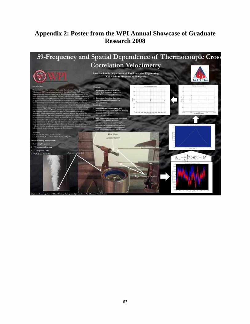
63

Appendix 2: Poster from the WPI Annual Showcase of Graduate

Research 2008

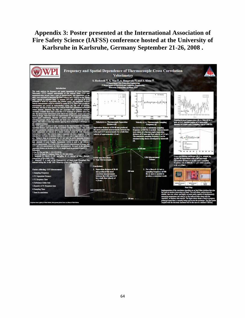
64

Appendix 3: Poster presented at the International Association of

Fire Safety Science (IAFSS) conference hosted at the University of

Karlsruhe in Karlsruhe, Germany September 21-26, 2008 .