an investigation into the energy consumption of future

Department of Mechanical Engineering

An Investigation into the Energy Consumption of Future

Office Buildings around the world

Author: James Johnston

Supervisor: Professor John Counsell

A thesis submitted in partial fulfilment for the requirement of degree in

Master of Science in Energy Systems and the Environment

2009

Copyright Declaration

This thesis is the result of the author’s original research. It has been composed by the

author and has not been previously submitted for examination which has led to the award

of a degree.

The copyright of this thesis belongs to the author under the terms of the United Kingdom

Copyright Acts as qualified by University of Strathclyde Regulation 3.50. Due

acknowledgement must always be made of the use of any material contained in, or derived

from, this thesis.

Signed: James Johnston Date: 18th

September 2009

1 Acknowledgements

I would like to thanks my parents for taking care of me over the summer, my supervisor for

his guidance and my girlfriend for her support and belief in me.

2 Abstract

Many of the studies into building energy consumption focus on optimizing a small detail

rather than looking at the whole. This study was undertaken at a higher level and looked

into a wide range of possible influences on the energy consumption – to build up a realistic

profile for a future office.

The first element under investigation is the evolving flexible workplace strategy.

The trend towards a more distributed and mobile workforce have implications on both

occupancy gains in the space and IT equipment use. In order to fully appreciate the impact

of a ubiquitous workforce, an occupancy profile generator tool was developed. This tool

could be used for different proportions of office workers – fulltime onsite workers,

telecommuters and mobile workers. Three workplace scenarios were developed to

investigate a) business as normal b) increased teleworking and c) a future workplace. It was

discovered that one of the most effective ways of reducing the energy consumption is

simply encouraging the use of laptops instead of desktop computers.

A total energy simulation was then run on a 6 floor low-rise building in central

London. A hybrid modelling approach was undertaken; using ESP-r for the thermal loads

and developing excel spreadsheets for analysing the IT, lighting and HVAC loads.

Scenarios were created, based on definitions from Carbon Trust typical and good practice

benchmarks and compared with a theoretical future office. The results of the study show

that energy consumption could be potentially reduced by 70% in 10 years time.

The potential for using photovoltaic solar power was then examined. An analysis

into optimal tilt angles for roof based panels was undertaken to investigate the sensitivity of

shading effects from adjacent panels. It was concluded that horizontal panels provided the

maximum generation in a year.

Finally, a comparison of different worldwide locations, and the impact on the

energy demands and PV supply was undertaken. The results show that the temperate

maritime climate in north-west Europe is the least able to achieve carbon neutral, whilst

offices in Mediterranean or desert locations can be 90% off-grid.

3 Table of Contents

1 Acknowledgements........................................................................................................ 3

2 Abstract .......................................................................................................................... 4

3 Table of Contents........................................................................................................... 5

4 List of figures............................................................................................................... 10

5 List of tables................................................................................................................. 13

5 List of tables................................................................................................................. 13

6 Introduction.................................................................................................................. 14

6.1 Key trends and influences.................................................................................... 14

6.2 Summary and Scope ............................................................................................ 15

7 Flexible Working Styles in the Future Office.............................................................. 16

7.1 The “Flexible workforce Strategy”...................................................................... 16

7.1.1 Generation Y................................................................................................ 16 7.1.2 Alternative Working Styles.......................................................................... 17 7.1.3 Typical Workplace profiles.......................................................................... 19

7.2 Occupancy Density and Building Utilisation ...................................................... 20

7.2.1 Benchmark data summary............................................................................ 20 7.2.2 Seasonal and diurnal influence on occupancy density................................. 20 7.2.3 Sharing workspaces to increase building utilisation.................................... 22 7.2.4 Case Study: Shared workspaces at Ernst & Young LLP [23] ..................... 23

7.3 Simulating Daily Occupancy Behaviour ............................................................. 24

7.3.1 A framework for generating the profile ....................................................... 24 7.3.2 Modelling Uncertainties............................................................................... 26 7.3.3 Profile Verification ...................................................................................... 26

7.4 Flexible Workplace Study.................................................................................... 27

7.4.1 Scenario 1: Business as normal.................................................................... 28 7.4.2 Scenario 2: Encouraged tele-working and shared workspaces .................... 28 7.4.3 Scenario 3: The future office and a mobile society ..................................... 29

7.5 Analysis................................................................................................................ 29

8 The Impact on IT in the Future Office......................................................................... 30

8.1 Overview.............................................................................................................. 30

8.2 Influence on energy-use....................................................................................... 30

8.3 Simulating office equipment energy use.............................................................. 31

8.3.1 Summary of equipment density assumptions .............................................. 31 8.3.2 Power levels of office equipment ................................................................ 32 8.3.3 Power management of office equipment ..................................................... 33

8.4 Comparison and Analysis .................................................................................... 34

9 Lighting in the Future Office ....................................................................................... 37

9.1 Overview.............................................................................................................. 37

9.2 Daylight Design ................................................................................................... 37

9.3 Procedure ............................................................................................................. 39

9.3.1 Hour by hour average daylight factor analysis ............................................ 39 9.3.2 Control Strategies......................................................................................... 40 9.3.3 Electric Lighting Power Density.................................................................. 40 9.3.4 Modelling Uncertainties............................................................................... 41 9.3.5 Sensitivity Analysis ..................................................................................... 42

9.4 Results and Analysis ............................................................................................ 44

10 Modelling the HVAC requirements......................................................................... 46

10.1 Building a Speculative Office.............................................................................. 46

10.1.1 Introduction.................................................................................................. 46 10.1.2 Building aspect and dimensions................................................................... 46 10.1.3 Fabric Construction...................................................................................... 47

10.2 Modelling Procedure............................................................................................ 49

10.2.1 Modelling using ESP-r................................................................................. 49 10.2.2 Model Detail ................................................................................................ 50

10.3 HVAC system Design.......................................................................................... 53

10.3.1 Overview...................................................................................................... 53 10.3.2 Ventilation Strategy ..................................................................................... 53 10.3.3 Fan Power .................................................................................................... 55 10.3.4 Heat Recovery.............................................................................................. 56 10.3.5 Humidity control .......................................................................................... 57 10.3.6 Boiler Performance ...................................................................................... 58 10.3.7 Chiller Performance ..................................................................................... 58

11 Total Energy End-use Review ................................................................................. 60

11.1 Auxiliary Loads ................................................................................................... 60

11.1.1 Hot Water Energy Consumption.................................................................. 60 11.1.2 Lift Energy Consumption ............................................................................ 60 11.1.3 Catering........................................................................................................ 60


11.2.1 Typical Office .............................................................................................. 61 11.2.2 Good Practice............................................................................................... 61 11.2.3 Future ........................................................................................................... 62 11.2.4 Summary...................................................................................................... 62

11.3 Summary.............................................................................................................. 63

11.4 Verification and discussion.................................................................................. 63

12 PV Resource............................................................................................................. 64

12.1 Overview.............................................................................................................. 64

12.2 Photovoltaic Panels and Efficiency ..................................................................... 65

12.3 Geometry of Building and PV Panels.................................................................. 66

12.4 Optimum Tilt angle from first principles............................................................. 67

12.4.1 Modelling the Sun........................................................................................ 68 12.4.2 Direct Radiation on Horizontal and Vertical Surfaces ................................ 69 12.4.3 Direct Radiation on Tilted Panels ................................................................ 70 12.4.4 Diffuse Radiation ......................................................................................... 70

12.5 Optimum tilt for panels with local shading.......................................................... 71

12.5.1 Direct Beam Shading Coefficient ................................................................ 71 12.5.2 Diffuse Shading Coefficient ........................................................................ 72 12.5.3 Verification with ESP-r................................................................................ 74

12.6 Optimum Tilt Angle............................................................................................. 77

13 International Case Studies........................................................................................ 78

13.1 Rationale for choosing location ........................................................................... 78

13.1.1 Worldwide Trade and Commerce................................................................ 78 13.1.2 Worldwide Climate zones............................................................................ 79

13.2 Selecting the Sample Range................................................................................. 80

13.3 Building Scenarios ............................................................................................... 81

13.3.1 Scenario 1: Sheltered urban low-rise ........................................................... 81 13.3.2 Scenario 2: Semi-exposed downtown high-rise........................................... 83

13.4 PV Generation Potential ...................................................................................... 84

13.4.1 Optimal Tilt Angle....................................................................................... 84 13.4.2 PV Generation per building type ................................................................. 85

13.5 Energy Demand Comparison............................................................................... 86

13.5.1 Lighting........................................................................................................ 86 13.5.2 Demand Summary ....................................................................................... 87

13.6 Supply and Demand Matching............................................................................. 89

13.6.1 Battery Storage Assumptions....................................................................... 89 13.6.2 CHP analysis................................................................................................ 90


13.7.1 % of met demand with PV supply ............................................................... 92 13.7.2 Average electrical demand met by Renewable Source................................ 93 13.7.3 Excess sold back to the grid......................................................................... 94

13.8 Sensitivities .......................................................................................................... 94

13.8.1 Sensitivity 1: LED Efficacy......................................................................... 95 13.8.2 Sensitivity 2: Chiller Performance............................................................... 96

13.8.3 Sensitivity 3: PV efficiency ......................................................................... 97 14 Discussions .............................................................................................................. 98

14.1 The Flexible Workforce....................................................................................... 98

14.1.1 Discussion.................................................................................................... 98 14.1.2 Summary of Contributions........................................................................... 98 14.1.3 Analysis of Sensitivities............................................................................... 98 14.1.4 Results and Conclusions .............................................................................. 99

14.2 Ubiquitous Computing......................................................................................... 99

14.2.1 Discussion.................................................................................................... 99 14.2.2 Summary of Contributions......................................................................... 100 14.2.3 Results and Conclusions ............................................................................ 100

14.3 Future Lighting Systems .................................................................................... 101

14.3.1 Discussion.................................................................................................. 101 14.3.2 Summary of Contributions......................................................................... 102 14.3.3 Analysis of Sensitivities............................................................................. 103 14.3.4 Results and Conclusions ............................................................................ 103

14.4 HVAC systems................................................................................................... 103


14.5 PV Resource....................................................................................................... 106


14.6 Building Type .................................................................................................... 107


14.7 Worldwide Locations......................................................................................... 109

14.7.1 Demand Summary ..................................................................................... 109 14.7.2 PV Supply .................................................................................................. 109 14.7.3 Supply and Demand Matching................................................................... 109 14.7.4 Sensitivities ................................................................................................ 110

15 Summary................................................................................................................ 111

16 References.............................................................................................................. 112

17 Appendices............................................................................................................. 120

17.1 Appendix 1: Office equipment energy use ........................................................ 120

17.2 Appendix 2: Energy breakdown for each city ................................................... 124

17.2.1 London ....................................................................................................... 124 17.2.2 Chicago ...................................................................................................... 125 17.2.3 Los Angeles ............................................................................................... 126 17.2.4 Dubai.......................................................................................................... 127 17.2.5 Singapore ................................................................................................... 129

4 List of figures

Figure 1: The intertwining nature of technology and behaviour ......................................... 15

Figure 2: Summary of growth in alternative working styles in the UK, [20] ...................... 18

Figure 3: worker types as found in a survey across the US [21] ......................................... 19

Figure 4: Benchmark data comparison displayed by NAO [23].......................................... 20

Figure 5: Graph showing diurnal and seasonal variations in average occupancy density for

an office in Colorado in 1994/5 [25].................................................................................... 21

Figure 6: Seasonally averaged peak and average occupancy density [25, 27] .................... 22

Figure 7: How a building can be utilised more effectively (as shown by Harris) [16]........ 22

Figure 8: “More London – Ernst & Young HQ”, www.flickr.com, Creative Commons.... 23

Figure 9: Design condition and maximum measured data................................................... 26

Figure 10: Business as Usual occupancy density ................................................................ 28

Figure 11: Encouraged teleworking and shared workspaces ............................................... 28

Figure 12: Future mobile society and shared workspaces ................................................... 29

Figure 13: Scenario 1: Comparison of computer use between different workers................ 31

Figure 14: Scenario 2: Comparison of computer use between different workers................ 32

Figure 15: Business as normal scenario electrical IT demand............................................. 34

Figure 16: Flexible workforce scenario electrical IT demand ............................................. 34

Figure 17: Future scenario electrical IT demand ................................................................. 35

Figure 18: EUI comparison of IT scenarios......................................................................... 35

Figure 19: Employee Energy Use Index for IT ................................................................... 36

Figure 20: Examples of different sky types (from Sq1 research) [48] ................................ 37

Figure 21: Design sky exceedance curve for London.......................................................... 38

Figure 22: Optimum daily energy consumption ................................................................. 42

Figure 23: Bad Practice daily energy consumption ............................................................. 42

Figure 24: Theoretical monthly average .............................................................................. 42

Figure 25: Bad Practice monthly average............................................................................ 42

Figure 26: Theoretical % electric lighting ........................................................................... 43

Figure 27: Bad Practice % electric lighting ......................................................................... 43

Figure 28: Winter illuminance daily profile ........................................................................ 44

Figure 29: Summer illuminance daily profile...................................................................... 44

Figure 30: Comparison between typical and best practice daily lighting demand .............. 45

Figure 31: Plan of office floor ............................................................................................. 46

Figure 32: Office section (E. Kohn et al) [53] ..................................................................... 47

Figure 33: Perspective drawing of office............................................................................. 47

Figure 34: ESP-r heat flux balance in each zone ................................................................. 50

Figure 35 Comprehensive ESPr building model ................................................................. 51

Figure 36: Simple ESPr building model .............................................................................. 51

Figure 37: Monthly averaged heating and cooling loads of the building ............................ 52

Figure 38: Verification of single floor model ...................................................................... 52

Figure 39: VAV and CAV system diagram......................................................................... 54

Figure 40: Volume flow rate for CAV and VAV systems................................................... 55

Figure 41: Fan energy requirement comparison between the different office scenarios ..... 56

Figure 42: HVAC system with Heat recovery wheel in the Fresh Air Unit ........................ 56

Figure 43: Boiler Part-load performance ............................................................................. 58

Figure 44: Conventional chiller system COP ...................................................................... 58

Figure 45: Future chiller system COP ................................................................................. 59

Figure 46: COP variation throughout the year for the different office scenarios ................ 59

Figure 47: Typical office annual energy use........................................................................ 61

Figure 48: Good Practice annual energy use ....................................................................... 61

Figure 49: The three office scenarios annual energy use comparison ................................. 62

Figure 50: Carbon Trust Econ-19 office energy consumption benchmarks[38] ................. 63

Figure 51: Photovoltaic Solar Electricity Potential in European Countries [67]................. 64

Figure 52: Direct and Diffuse solar radiation components for London............................... 66

Figure 53: Explanation of solar azimuth and elevation [75]................................................ 68

Figure 54: North-south section explaining diffuse radiation on tilted panels...................... 70

Figure 55: Shading occurring on rooftop PV panels ........................................................... 71

Figure 56: Direct beam shading from adjacent panels (from Appelbaum et al. [73]) ......... 72

Figure 57: Diffuse beam shading impact from adjacent panels (from Passias et al. [72]) .. 73

Figure 58: Average masking angles vs. inclination angle for various values of C/A (=k).. 74

Figure 59: Roof PV layout................................................................................................... 74

Figure 60: Monthly direct beam shading coefficients using Excel...................................... 75

Figure 61: Monthly direct beam shading coefficients using ESP-r ..................................... 75

Figure 62: PV generation comparison between ESP-r and Excel for a London climate ..... 76

Figure 63: Global irradiation for panels at different tilt angles in London.......................... 77

Figure 64: MasterCard Centers of Commerce: Continental split ........................................ 78

Figure 65: World map of the Köppen-Geiger climate classification [81] ........................... 79

Figure 66: Building Height in Central London using IKONOS data [77]........................... 82

Figure 67: Fitzroy Street in London shading from trees and adjacent buildings [82] ......... 82

Figure 68: Details of urban low-rise scenario...................................................................... 82

Figure 69: View of Toronto downtown area........................................................................ 83

Figure 70: Downtown High-rise scenario details ................................................................ 83

Figure 71: Global irradiation for shaded panels in different world locations...................... 84

Figure 72: Global irradiation for unshaded panels in different world locations.................. 84

Figure 73: PV Generation opportunity for different building types around the world........ 85

Figure 74: External Diffuse Illuminance availability around the world .............................. 86

Figure 75: Monthly lighting energy demand comparison around the world ....................... 86

Figure 76: Electrical Demand per building type in each location ....................................... 87

Figure 77: Heating Demand per building type in each location .......................................... 87

Figure 78: High-rise Energy Use Index for each worldwide location ................................. 88

Figure 79: Low-rise Energy Use Index for each worldwide location.................................. 88

Figure 80: CHP for Space Heating Suitability..................................................................... 91

Figure 81: Low rise Building: % of electrical demand met with PV supply per month...... 92

Figure 82: High rise Building: % of electrical demand met with PV supply per month..... 92

Figure 83: Electrical demand met by PV supply (alone) per year ....................................... 93

Figure 84: Electrical demand met by PV and CHP per year ............................................... 93

5

List of tables

Table 1: Summary of Different AWS (Alternative Working Styles) options ..................... 17

Table 2: worker types as found in a survey across the US .................................................. 19

Table 3: Example organisations which are adopting workspace sharing [22]..................... 23

Table 4: % of working days in the office per year by employees........................................ 25

Table 5: % of working days in the office per year by visitors............................................. 25

Table 6: Summary of profile generation assumptions ......................................................... 25

Table 7: Summary of office layout scenarios ...................................................................... 27

Table 8: Detailed overview of worker profiles for each scenario........................................ 27

Table 9: Summary of Power Consumption of IT equipment............................................... 32

Table 10: Summary of power management in IT equipment .............................................. 33

Table 11: Summary of lighting use assumptions................................................................. 43

Table 12: Summary of results for each office scenario ....................................................... 44

Table 13: Summary of glazing assumptions........................................................................ 48

Table 14: Constructions Summary....................................................................................... 49

Table 15: Infiltration Summary ........................................................................................... 49

Table 16: ESP-r zone temperature and humidity set-points ................................................ 50

Table 17: HVAC systems overview .................................................................................... 53

Table 18: Hot Water Energy Consumption ......................................................................... 60

Table 19: Summary of expected PV efficiencies in 2030 [68] ............................................ 65

Table 20: Symbols used in solar angle calculations ............................................................ 67

Table 21: PV generation comparison between ESP-r and Excel for a London climate ...... 76

Table 22: MasterCard Centers of Commerce: Top ten cities .............................................. 78

Table 23: Comparison between the climates of world cities ............................................... 81

Table 24: Optimal PV tilt angle in different worldwide locations....................................... 84

Table 25: PV opportunity per building type ........................................................................ 85

Table 26: Summary of electric lighting requirement around the world............................... 87

Table 27: CHP for Hot Water summary .............................................................................. 90

6 Introduction

A major influence on the way offices will be used in the future is the increasing importance

of sustainability – primarily with the need to reduce carbon emissions to mitigate the

impact of anthropogenic climate change. Whilst an important factor now, by 2020 it will

require more than awareness to meet the difficult carbon emission reduction targets set by

our government and the EU [1].

The second trend is a behavioural change in how employees perceive their

worksetting. Through the rapid progression of mobile communication devices, the era in

which the office can be seen as a static place for individual work is over [2]. Employers

and employees are finding that a more distributed approach to work can allow for a better

work-life balance, and the increased independence actually increases productivity [3].

Reducing the number of hours travelling per week also reduces the carbon footprint of the

commute [4].

6.1 Key trends and influences

This behavioural change is impacting the requirements of the office worksetting, in which

fixed places for quiet work will be seen as auxiliary space, rather than the main purpose.

Instead, offices will be seen as hubs for collaborative work and will require an extremely

flexible and independent layout [5]. The technical challenges facing this new office

environment are not insurmountable but do require some innovative solutions. The first

challenge is with the “nervous system” of the building – the electrical network.

In the future office, almost all the electrical loads will be entirely unsuited to the

high voltage alternating current (AC) network which is currently available. Instead all low-

powered laptops, mobile devices, LED lighting and other office equipment will run on low

voltage direct current (DC) power [6].

The intertwining nature of technology and behavioural trends are displayed in the

diagrammatic in Figure 1.

Figure 1: The intertwining nature of technology and behaviour

The figure demonstrates how the biggest electrical demands – cooling, lighting and

computing can all be integrated using a DC network.

A central theme in the office of the future is generating electricity onsite using PV

panels. To date, PV generation is seen as an inefficient and expensive method of electricity

generation – however it is widely acknowledged that in a few decades, the cost

effectiveness of installing and running PV could equal that of conventional means [8].

6.2 Summary and Scope

There are many elements of uncertainty in the design and operation of a future

office, but most predominately;

• Behaviour Trends: how it is used by the occupants and how this is changing

• Advances in technology: the extent to which the building fabric and building

systems will improve in the future

• Environment: the location in which the office is based.

7 Flexible Working Styles in the Future Office

Advances in communication, transportation and the trend towards a globalised and

connected world are having a major impact in the office place. The three most influential

trends are:

• the rapid expansion of the services industry, bringing ever more information work and the evolution of a creative economy [4]

• the development of a distributed work strategy with mobile and flexi-time workers [10]

• the increased awareness and sense of duty to mitigating environmental impact [11]

7.1 The “Flexible workforce Strategy”

7.1.1 Generation Y

The creative economy is the most dominant force in innovation and progress in the

business world today. Whilst at the start of the 20th century, less than 10% of the working

population focused on creative work such as the science and technology, cultural, and

knowledge based industries such as law and medicine– in the last few decades this has

risen to over 30% [12]. This has implications on our fundamental understanding of why we

work in the first place. Davis et al. [3] argues that we have left behind the old-fashioned

concept of work being as a form of punishment, and that now concepts such as work-life

balance are becoming core requirements of the workforce.

In Post Fordist economies, effective communication networks are the pillars on

which innovation and positive growth rely [2]. This need for effective communication is

driven by Generation Y or Gen Y, defined as those who were born post 1980s and have all

grown up with instant messaging, mobile phones and laptops. DEWG, a think-tank for the

design of future offices, describes Gen Y as being independent, progressive, international

and entrepreneurial [5]. Brought up in the age of Web 2.0 and open source, they are not

accepting the strictly hierarchical and authoritarian rules of the traditional work place and

instead are open to sharing ideas through mass collaboration [13].

We are entering a period where we have access to the sum of the world’s

knowledge and simultaneously are able to effectively communicate it to anyone in the

world, anytime and anywhere [14]. There is a growing feeling amongst organisations that

mass collaboration over the internet is not just a fad, and it is crucial that they can update

their business plan to be more receptive to this new way of thinking. An essential

component of this open approach is in how large organisations, which dominated the

business world of the 20th century, will treat their employees in the future. Some have

already adopted a far more open and flexible approach, such as IBM and Nokia with

considerable success, encouraging others to follow in their footsteps [13, 15].

7.1.2 Alternative Working Styles

“Alternative working styles” [16] is one of the many ways of defining the new

workplace strategies – amongst other words, such as “distributed working” and “flexi-

working” [4]. It encompasses a range of alternative solutions for the workplace without

focusing on one particular strategy – as summarised in the table below:

Type of AWS Typical Description [17]

Part time Increasingly popular - 2.2 million in 1970 to 7 million today (and mostly out of choice rather than necessity)

Job Share Where one job is shared by 2 people. (Often 2 part-time workers are more productive than one full-time.)

Annualised Hours

Total number of annual hours is agreed, and then employee is free to complete them as they like. (Can do "two week, two off" etc)

Flexitime Core hours – perhaps from 10am until 3pm or 4pm, then free to choose how to add hours either side.

Compressed working week

4 day week (10 hour days) 9 day fortnight (4 days, working 9 hours, on the 5th day 8hours one week, and free the next)

Teleworking Defined as working from home, on the move or from telecentres or satellite offices – and requiring advanced telecoms to work

Table 1: Summary of Different AWS (Alternative Working Styles) options

The benefits of flexible working practices on the well-being of the worker are well

documented [18]. The government fully supports these as an important aspect of the work-

life balance: in a study (2007) they found that with better work-life balance, employers

enjoyed better relations with their employees, received improved commitment and

motivation and a lower staff turnover [19].

A CIB report carried out on a cross section of 5000 companies showed that in all

aspects – the availability of these flexible work choices (both written and informal

agreements) has been increasing over the last 4 years [20].

0%

10%

20%

30%

40%

50%

60%

70%

80%

90%

100%

Part-time work Job sharing Flexitime Annualised

hours

Telework Compressed

hours

Ty

pe

of

fle

xib

le w

ork

ing

arr

an

ge

me

nts

off

ere

d b

y U

K e

mp

loye

rs (

%)

2004

2005

2006

2007

Figure 2: Summary of growth in alternative working styles in the UK, [20]

However, the Equal Opportunities Commission discovered in a study (2007), that there is

an unmet need for flexible work styles in the UK, with key findings such as:

• 4.8 million feel their skills in their current job are underutilised but find it difficult

to change jobs because of the lack of flexibility in the workplace

• Evolution of equal rights in the family: between 2000 and 2005, the number of

fathers teleworking from home rose from 14% to 29%

• 50% of all working adults said they want more flexibility in their job

• But 60% said they had not been exposed to any information on flexible working

options

The report uncovered that even though the availability of flexible working was increasing,

the demand still greatly outweighs supply in flexible working practices [18]. In the future

we will see more and more of these alternative approaches to working and with it, different

requirements on the office environment.

7.1.3 Typical Workplace profiles

The cultural movement towards flexible working styles brings with it a more

ubiquitous or mobile workforce. Some studies have been done on current levels of

ubiquitous working practices in the office place.

A. Richman et al. [21] undertook a survey to define the real levels of mobility in

modern US offices. They used a large sample size of 2057 full-time US employees from

over 500 private companies. They defined workers into the different categories: “On-site

worker”, “Ad-hoc tele-worker”, “Regular Tele-worker”, “Mobile worker”, “Remote

worker” and “Customer Site worker”. The proportion of each worker and an explanation of

each category are explained in the chart and table below.

On-site worker

50%

Ad-Hoc Tele-Worker

15%

Regular Tele-worker

7%

Remote Worker

4%

Mobile Worker

12%

Customer Site

Worker

12%

Figure 3: worker types as found in a survey across the US [21]

• Onsite workers: Traditional worker who does not work from home during regular office hours.

Only occasionally leaves the office for meetings.

• Ad-hoc tele-workers: Similar to onsite workers, but work from home at least once a month

• Regular tele-workers: Work primarily in the office, but work from home at least 3 days a

fortnight.

• Remote workers: Work based at home full-time, and only occasionally visit the office for

administration purposes and meetings

• Mobile workers: perform their work in a number of locations, but do still spend a few days a

week in the office.

• Customer Site workers: work full time at their project site, occasionally visiting the office

Table 2: worker types as found in a survey across the US

7.2 Occupancy Density and Building Utilisation

7.2.1 Benchmark data summary

Occupancy density (OD) is normally calculated by dividing the net internal floor area by

the total number of employees allocated to the building [24].

An IPD report for the Office of Government Commerce looked at all available

sources for benchmark data for occupancy density. There was a general consensus that

around 14-16m2/person was typical, and at most 12-20m2/person [22]. This is displayed in

graphical form in a report for the National Audit Office, as seen in Figure 4 [23].

Figure 4: Benchmark data comparison displayed by NAO [23]

7.2.2 Seasonal and diurnal influence on occupancy density

Whilst these details on benchmark and good practice occupancy density (OD) are

widespread, they are normally a calculation of workspace density rather than an actual

account of how many occupants are in the office at one time. Real data on OD for offices in

the UK, taking into account both seasonal and diurnal variations are difficult to find [16].

The author deemed it acceptable to use real OD data from an office from the US, as the

most important variations in occupancy behaviour would occur between different office

types and not from the office location [21]. Keith [25] took readings of the peak and

average OD throughout a standard 9am-5pm workday, each month from October 1994 to

September 1995 at the offices for the National Center for Atmospheric Research (NCAR)

in Boulder, Colorado. It is a research and academic institute consisting of a campus of three

small buildings, a total of around 1200 rooms and an individual occupancy sensor in each

room. Keith used a sample size of 97 rooms, and did not include rooms that were

unallocated (permanently unoccupied). Each occupancy sensor had a binary output of

either: “occupant detected” or “occupant not detected”.

Figure 5: Graph showing diurnal and seasonal variations in average occupancy density for an office in

Colorado in 1994/5 [25]

As seen in Figure 5 there is a clear diurnal and seasonal variation in OD, so that

whilst the benchmark value will be useful in determining maximum conditions (used for

design of the building services [26]) it is not appropriate for simulations on total annual

energy consumption.

To simplify the data set, the average and peak OD were seasonally averaged. These

are shown in Figure 6along with the widely recognised design OD from ASHRAE

Standard 90.1-2007 [27]. It is immediately noticeable that the guideline values – at a nearly

constant 95% occupancy are far away from the actual density. The average density only

reaches a maximum of 57% with a peak of 65%.

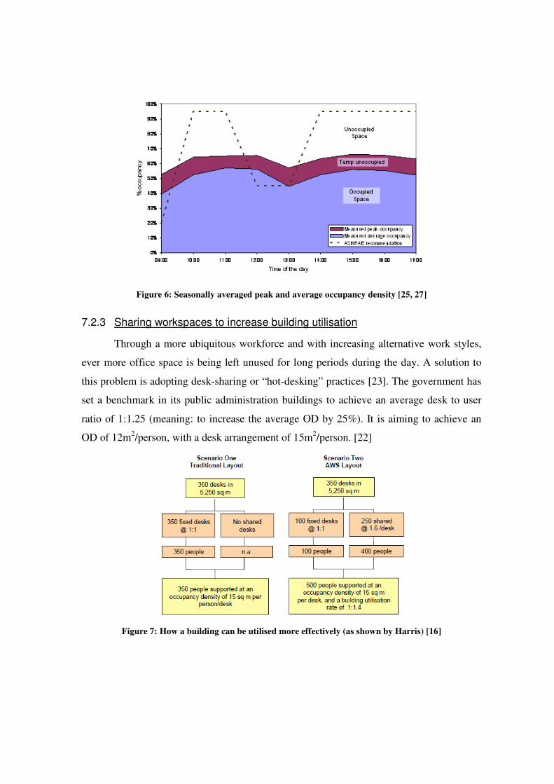
Figure 6: Seasonally averaged peak and average occupancy density [25, 27]

7.2.3 Sharing workspaces to increase building utilisation

Through a more ubiquitous workforce and with increasing alternative work styles,

ever more office space is being left unused for long periods during the day. A solution to

this problem is adopting desk-sharing or “hot-desking” practices [23]. The government has

set a benchmark in its public administration buildings to achieve an average desk to user

ratio of 1:1.25 (meaning: to increase the average OD by 25%). It is aiming to achieve an

OD of 12m2/person, with a desk arrangement of 15m2/person. [22]

Figure 7: How a building can be utilised more effectively (as shown by Harris) [16]

There is growing evidence that organisations are adopting workspace sharing to increase

the building utilisation. Examples can be seen in all industry sectors:

OrganisationTreated Floor

Area (m²)

Number of

Employees% at 1:1

% sharing

workspaces

Shared Workspace

Ratio

(Desk:employee)

Average Building

Utilisation

Adult Learning Inspectorate 1,862 282 51% 49% 10:1 1.9

BAA 4,333 540 10% 90% 1.2:1 1.2

BP 41,209 4445 0% 100% 1.2:1 1.2

BT 26,500 4000 38% 63% 8.3:1 2.2

Cambridgeshire County Council 1,185 112 53% 47% 1.2:1 1.1

Dti 20,000 1600 0% 100% 1.3:1 1.3

Ernst & Young 37,800 4200 65% 35% 3:1 1.3

GCHQ 5,900 4900 0% 100% 1.5:1 1.2

Hertfordshire County Council 10,220 1000 0% 100% 3:1 1.3

IBM 15,525 1473 62% 38% 3.4:1 1.9

Norfolk county council 1,135 165 82% 18% 2.5:1 1.1

PricewaterhouseCoopers 9,316 1750 20% 80% 1.3:1 2.6

Suffolk County Council 13,286 1150 77% 23% 1.3:1 1.2Sun Microsystems 25,220 1717 21% 79% 1.6:1 1.4

Table 3: Example organisations which are adopting workspace sharing [22]

7.2.4 Case Study: Shared workspaces at Ernst & Young LLP [23]

Figure 8: “More London – Ernst & Young HQ”, www.flickr.com, Creative Commons

When Ernst & Young moved their headquarters in 2003, they downsized from 9

offices to just 2; halving the required floor area whilst retaining the same number of

employees. They was achievable by actively encouraging tele-working and mobile working

practices, and by implementing a 1:3 worker:desk ratio for 35% of their employees.

Along with this flexible work strategy, 80% of their staff use laptops and shelves

were placed at a distance from the workstations to discourage “local nesting”. To reduce

the energy footprint of the office further, they have adopted highly efficient scanners,

copiers and printers at a density of 1 machine per 50 staff.

Crucial to the success of their new head quarters is the concept of “spaceless

growth” where a company does not have to acquire new space to house larger numbers of

employees. The reported also discovered that 19% of workspaces in all government

buildings remain unallocated because of the inflexible approach of being able to scale the

lease. The new flexible work strategy relies on short term and scalable leases which can

mean office space can be used far more effectively [28]. DEWG claim that 66% of their

clients will not be renewing their leases after the current one runs out, suggesting that the

idea of flexible leases will really become mainstream [29].

7.3 Simulating Daily Occupancy Behaviour

7.3.1 A framework for generating the profile

Occupancy behaviour plays an important role in calculating the casual gains and IT

equipment demands in the space. As was discussed in section 7.2.2, there is limited

quantitative understanding on actual occupancy density in offices. Hence it was necessary

to develop a tool to generate a daily occupancy profiles which then could be varied

depending on the number of mobile, semi-mobile and fixed workers.

As occupancy density is not yet a well defined science, there are many different

descriptions of the same types of worker: so for the purposes of this study the definitions

consistent with those written by Richman et al [21] will be used, but could be changed if

necessary. The five types of worker are “Onsite worker”, “Ad-hoc teleworker”, “Regular

teleworker”, “Remote worker”, “mobile worker” and “customer site worker” (please see

section 7.1.3 for further description of each type). For simplification, the customer site

workers have been combined with the data for remote workers, due to the small number of

days each work on site.

To generate a total occupancy graph for a certain combination of workers – the

characteristics of each type had to be defined in terms of:

• % of working year spent on holiday

• % of working days per year in the office. (Source used: Richman et al [21])

• Arrival time in the office. (Source used: Lehmann et al [4])

• Average length of working day. (Source used: Richmann et al)

Excluding bank holidays when the office would be shut anyway, an employee is entitled to

20days annual leave, which means only 92% of working year is spent working. This value

was then multiplied by the % of total working hours that are spent in the office for each

type of worker (93% for onsite workers down to 9% for remote workers) to find the overall

% of working days spent onsite. Onsite workers spend actually only 86% of working days

in the office, and this can be as low as 35% for mobile workers.

Employees of the Organisation

Worker Type working days/ month onsite

working days in a year (total)

working days/ year onsite

% of working days onsite

On-site worker 20.3 260 224 86%

Ad-Hoc Tele-Worker 19.3 260 214 82%

Regular Tele-worker 13.8 260 153 59%

Remote Worker 1.95 260 21 8%

Mobile Worker 8.1 260 90 35%

Table 4: % of working days in the office per year by employees

All of these workers types spend some of their off-site time at another company

site. Assuming that this will be reciprocated by these other companies; it is necessary to

model the impact of visitors that require workspaces too.

Visitors to the Organisation

Visitor Type working days/ month onsite

working days in a year (total)

working days/ year onsite


On-site worker 0.3 260 3 1%

Ad-Hoc Tele-Worker 0.6 260 7 3%

Regular Tele-worker 0.4 260 4 2%

Remote Workers 0.3 260 3 1%

Mobile Worker 2.6 260 31 12%

All Visitors 3.9 260 45 18%

Table 5: % of working days in the office per year by visitors

Worker Type Daily Working

hours [21] Arrive

time [4] Departure

time


On-site worker 9 hours 8am 5pm 93%

Ad-Hoc Tele-Worker 9.5 hours 8am 5:30pm 89%

Regular Tele-worker 10 hours 8am 6pm 63%

Remote workers 9 hours 9am 6pm 8%

Mobile Worker 10.5 hours 9am 7:30pm 37%

All Visitors 9 hours 9am 6pm 18%

Table 6: Summary of profile generation assumptions

7.3.2 Modelling Uncertainties

To model the affect of a distributed arrival time (employees will not arrive at exactly the

same time), a time-offsetting variable was randomly allocated to each worker: -30mins,

0mins or +30mins. This does not affect the overall time spent at the office for each worker,

but achieves a more realistic smoothing-off of occupancy levels at the start and end of the

day.

To model occupants leaving the office at lunchtime, a 30% decrease in occupancy

density is implemented between the hours of 12pm-1pm. The distributed arrival time

algorithm means that this dip at lunchtime is also slightly more distributed.

7.3.3 Profile Verification

Using the above assumptions, the occupancy density profile was created as seen in Figure

9. For validation it was compared against the maximum values of occupancy (between the

hours of 9am and 5pm) as was measured by Keith [25] in the office in Colorado. There

seems to be a good match between the levels, again underlining the fact that 25% of the

office is empty even during peak hours.

0%

10%

20%

30%

40%

50%

60%

70%

80%

90%

100%

07:0

0

07:3

0

08:0

0

08:3

0

09:0

0

09:3

0

10:0

0

10:3

0

11:0

0

11:3

0

12:0

0

12:3

0

13:0

0

13:3

0

14:0

0

14:3

0

15:0

0

15:3

0

16:0

0

16:3

0

17:0

0

17:3

0

18:0

0

18:3

0

19:0

0

19:3

0

20:0

0

20:3

0

Time of the Day

% O

cc

up

an

cy

Profile Generator Results

Measured data (Peak)

Figure 9: Design condition and maximum measured data

7.4 Flexible Workplace Study

Three different profiles were generated to simulate different scenarios of flexible and

ubiquitous working styles. A base of 100 work stations was used.

1. Business as usual: the base case. 95 employees at fixed desks, and 5 “hot-desks”

for the occasional remote workers and visitors.

2. Tele-working workforce: working from is actively encouraged as a company

policy. 40 employees at fixed desks, and 60 desks at a desk: worker ratio of 2.5 to 1.

3. Mobile workforce: a future scenario where mobility is key, and the office is seen

as mainly a place for collaborative work. 23 fixed desks and 77 flexible desks at a

desk: worker ratio of 3.1 to 1.

Quantity Ratio Quantity Ratio Quantity Ratio

Permanent- desks 95 @ 1:1 40 @ 1:1 23 @ 1:1

Flexi- desks 5 @ 8.3:1 60 @ 2.5:1 77 @ 3.1:1

Total 100 @ 1.3:1 100 @ 1.9:1 100 @ 2.5:1

Business as usualScenario 1: Tele-working

workforce

Scenario 2: Mobile

workforce

Table 7: Summary of office layout scenarios

The table holds a detailed overview of the number of workers at each type of desk.

Onsite workers 57 Onsite workers 11 Onsite workers 11

Ad-hoc tele-workers 17 Ad-hoc tele-workers 28 Ad-hoc tele-workers 11

Regular tele-workers 8

Mobile workers 14

Subtotal 95 Subtotal 40 Subtotal 23

Remote workers 18 Regular tele-workers 74 Regular tele-workers 53

Visitors 17 Mobile workers 30 Mobile workers 93

Remote workers 18 Remote workers 18

Visitors 32 Visitors 72

Subtotal 35 Subtotal 153 Subtotal 236

Total 131 Total 193 Total 259

Increase 0% Increase 48% Increase 98%

Business as usual Scenario 1: Tele-working workforce Scenario 2: Mobile workforce

Permanent - desk

Flexi-desk

Permanent - desk

Flexi-desk Flexi-desk

Permanent - desk

Table 8: Detailed overview of worker profiles for each scenario

7.4.1 Scenario 1: Business as normal

0%

10%

20%

30%

40%

50%

60%

70%

80%

90%

100%

07:0

0

07:3

0

08:0

0

08:3

0

09:0

0

09:3

0

10:0

0

10:3

0

11:0

0

11:3

0

12:0

0

12:3

0

13:0

0

13:3

0

14:0

0

14:3

0

15:0

0

15:3

0

16:0

0

16:3

0

17:0

0

17:3

0

18:0

0

18:3

0

19:0

0

19:3

0

20:0

0

20:3

0

% O

ccu

pa

ncy

(w

ork

sp

ac

es

)

Remote Workers Visitors Mobile Workers

Regular Tele-workers Ad-Hoc Tele-Workers On-site workers

Figure 10: Business as Usual occupancy density

7.4.2 Scenario 2: Encouraged tele-working and shared workspaces

0%

10%

20%

30%

40%

50%

60%

70%

80%

90%

100%

07:0

0

07:3

0

08:0

0

08:3

0

09:0

0

09:3

0

10:0

0

10:3

0

11:0

0

11:3

0

12:0

0

12:3

0

13:0

0

13:3

0

14:0

0

14:3

0

15:0

0

15:3

0

16:0

0

16:3

0

17:0

0

17:3

0

18:0

0

18:3

0

19:0

0

19:3

0

20:0

0

20:3

0

% O

cc

up

an

cy

(w

ork

sp

ace

s)



Figure 11: Encouraged teleworking and shared workspaces

7.4.3 Scenario 3: The future office and a mobile society

0%

10%

20%

30%

40%

50%

60%

70%

80%

90%

100%

07:0

0

07:3

0

08:0

0

08:3

0

09:0

0

09:3

0

10:0

0

10:3

0

11:0

0

11:3

0

12:0

0

12:3

0

13:0

0

13:3

0

14:0

0

14:3

0

15:0

0

15:3

0

16:0

0

16:3

0

17:0

0

17:3

0

18:0

0

18:3

0

19:0

0

19:3

0

20:0

0

20:3

0

% O

cc

up

an

cy

(w

ork

sp

ace

s)



Figure 12: Future mobile society and shared workspaces

7.5 Analysis

Increasing the number of shared workspaces and encouraging more mobile and tele-

workers is a very easy way to increase the building utilisation and achieve spaceless

growth. The case studies show that it is not only possible, but is becoming a widespread

practice amongst organisations around the world.

As seen in scenario 2; by encouraging more regular tele-working, which is only 3

days at home a fortnight, and using more shared workspaces – a 48% increase in building

utilisation is possible.

In the future scenario, with 93 mobile workers – who all use the office only 2 days a

week – a 98% increase in building occupancy is possible.

8 The Impact on IT in the Future Office

8.1 Overview

IT consumption in modern offices is often very large – accounting for 16% of the total

electrical consumption. It can rise as high as 40% if there are dedicated computer rooms in

the office [38]. This does not even take into account the impact on the cooling requirement;

as all the electrical energy put into a computer ultimately convects and radiates into the

space as heat.

There have been many studies on the energy consumption of office equipment,

especially by the Lawrence Berkeley National Laboratory in the US [30, 31, 32, 33]. A

summary of these studies can be seen in appendix 17.

8.2 Influence on energy-use

One of the biggest challenges lies with improving the energy efficiency of desktop

computers. All the studies which have investigated actual power consumption, usage

patterns and night-time switch-off rates in typical offices show that desktop PCs perform

the poorest relative to all the other technologies.

In addition, 50- 60% of desktop computers were found to be left in a high power

state over night, compared with only 20-30% of monitors and 25% of laptops. What

accentuates this problem more is the fact that desktop computers use the most power; and

whilst trends in laptops and monitors are showing that power is reducing with time, the

opposite is true with PCs. They are certainly getting more efficient in how they use their

power, but the continually growing hardware demands from applications overrides this

positive influence.

Perhaps the biggest influence on the energy consumption of IT equipment is with

managerial policy. In the Ernst & Young case study, it was clear that a policy of giving out

laptops to 80% of staff– will eradicate all the challenges associated with improving the

energy efficiency of PCs. Laptops are inherently low-power, and the trends are still towards

reducing this; to maximise the battery life and hence mobility of the device.

8.3 Simulating office equipment energy use

The energy consumption of office equipment has been simulated for the three different

scenarios as defined in the flexible workplace strategy.

• Scenario 1: “business as normal” – representing an office with poor building

utilisation, with high power consumption and poor energy management

• Scenario 2: “flexible workforce” – representing a company that has adopted a

shared workspace strategy, along with using more laptops

• Scenario 3: “Future workforce” – representing a future, far more mobile workforce.

Power management is optimal and power levels are much lower. Most employees

use low power notebooks

8.3.1 Summary of equipment density assumptions

In the studies on equipment density for typical offices, there seems to be little

correlation between laptop use, suggesting that it is very dependent on the country and type

of application of the office. The most conservative estimate is that 10% of all computers

are laptops [37], and the most wild is 50% [21]. Other estimates are in between at 15% for

the US and 42% for Japan [35]. A middle value of 25% was assumed. Richmann et al [21]

have shown that laptop and desktop ownership depends on the role of the employee in the

company, as seen in Figure 13 and Figure 14.

0% 10% 20% 30% 40% 50% 60% 70% 80% 90% 100%

On-site worker

Ad-Hoc Tele-Worker

Regular Tele-worker

Mobile Worker

Remote Worker

Visitor

% ownership of technology

Laptop computer Desktop computer Figure 13: Scenario 1: Comparison of computer use between different workers

For the future scenario, it is assumed that 80% of employees have ownership of

laptops [23] and do not require the use of a desktop computer.

0% 10% 20% 30% 40% 50% 60% 70% 80% 90% 100%

On-site worker

Ad-Hoc Tele-Worker

Regular Tele-worker

Mobile Worker

Remote Worker

Visitor

% ownership of technology

Laptop computer Desktop computer Figure 14: Scenario 2: Comparison of computer use between different workers

In scenario 1, auxiliary equipment density has been taken from the study by Kawamoto et

al [35], where laser printers are shared by 6 employees and Fax, Scanner and Photocopier

machines are shared by 16 employees on average. In 2nd scenario, as adopted in Ernst &

Young, it is assumed that each machine is shared by 50 employees [23].

8.3.2 Power levels of office equipment

Power levels of equipment for the first two scenarios (current technology) and the third

scenario (future technology) have been catalogued in the following table [30, 32and 37].

Scenario Equipment Description On (W) Idle (W) Off (W)

Current Laptop 19 3 2

Desktop 70 9 3

CRT screen 63 2 1

Printer 278 27 11

Copier 1354 396 34

Fax 30 15 15

Scanner 150 15 0

Future Laptop 15 3 2

Desktop 60 9 3

LCD screen 17 2 2

Multifunctional machine 720 48 0

Table 9: Summary of Power Consumption of IT equipment

8.3.3 Power management of office equipment

The final aspect of simulating office equipment behaviour is looking into the typical power

management of each device. It can be seen that desktop computers in the current scenarios

are the worst performers – in which 55% of machines are left in high power state overnight.

During the daytime they also are the worst performers –whilst laptops and screens often

employ an efficient level of power management, very little is done in desktop computers

[30, 33 34]. In the future scenario, it is assumed that power management in desktops has

been improved and effective organisational policy has been implemented.

Scenario Equipment Description

Daytime (10 hours) Night time (remaining 14 hours)

High Low Off High Low Off

Current Laptop 55% 22% 23% 10% 0% 90%

Desktop 77% 0% 23% 55% 3% 42%

CRT screen 55% 22% 23% 30% 40% 30%

Printer 7% 93% 0% 0% 100% 0%

Copier 10% 90% 0% 0% 100% 0%

Fax 2% 98% 0% 0% 100% 0%

Scanner 2% 98% 0% 0% 100% 0%

Future Laptop 55% 22% 23% 0% 0% 100%

Desktop 55% 22% 23% 0% 0% 100%

LCD screen 55% 22% 23% 0% 0% 100%

Multifunctional

machine 17% 83% 0% 0% 0% 100%

Table 10: Summary of power management in IT equipment

8.4 Comparison and Analysis

Given a workspace density of 15m2/workspace, the three different scenarios were

compared.

0

1

2

3

4

5

6

7

8

9

10

00:0

0

01:0

0

02:0

0

03:0

0

04:0

0

05:0

0

06:0

0

07:0

0

08:0

0

09:0

0

10:0

0

11:0

0

12:0

0

13:0

0

14:0

0

15:0

0

16:0

0

17:0

0

18:0

0

19:0

0

20:0

0

21:0

0

22:0

0

23:0

0

Time of the day

Ele

ctr

ical

Po

wer

Dem

an

d W

/m2

CRT Screen

Desktop PC

Laptop

Office Equipment

Figure 15: Business as normal scenario electrical IT demand

0

1

2

3

4

5

6

7

8

9

10

00:0

0

01:0

0

02:0

0

03:0

0

04:0

0

05:0

0

06:0

0

07:0

0

08:0

0

09:0

0

10:0

0

11:0

0

12:0

0

13:0

0

14:0

0

15:0

0

16:0

0

17:0

0

18:0

0

19:0

0

20:0

0

21:0

0

22:0

0

23:0

0

Time of the day

Ele

ctr

ica

l P

ow

er

De

ma

nd

W/m

2

CRT Screen

Desktop PC

Laptop

Office Equipment

Figure 16: Flexible workforce scenario electrical IT demand

0

1

2

3

4

5

6

7

8

9

10

00:0

0

01:0

0

02:0

0

03:0

0

04:0

0

05:0

0

06:0

0

07:0

0

08:0

0

09:0

0

10:0

0

11:0

0

12:0

0

13:0

0

14:0

0

15:0

0

16:0

0

17:0

0

18:0

0

19:0

0

20:0

0

21:0

0

22:0

0

23:0

0

Time of the day

Ele

ctr

ica

l P

ow

er

De

man

d W

/m2

LCD Screen

Desktop PC

Laptop

Office Equipment

Figure 17: Future scenario electrical IT demand

A summary of the three scenarios is shown in the figure below. It is immediately apparent

that the energy consumption of IT in the future can be dramatically less than it is currently.

An 80% reduction is possible, even with the increased building utilisation. This accounts

for saving 320tonnes of carbon a year, for a typical 6 floor office.

0

5

10

15

20

25

30

35

40

45

50

Business as normal Flexible workforce Future scenario

kW

h/m

2 p

er

ye

ar

Auxiliary Equipment

Monitor

Desktop PC

Laptop

Figure 18: EUI comparison of IT scenarios

Perhaps a more consistent way to compare the performance of each office is to use show

the energy consumption per employee rather than per m2. This will show that the future

scenario actually consumes much less energy whilst having double the employees.

0

100

200

300

400

500

600

Business as normal Flexible workforce Future scenario

kW

h/e

mp

loyee p

er

ye

ar

Auxiliary Equipment

Monitor

Desktop PC

Laptop

Figure 19: Employee Energy Use Index for IT

This underlines the importance of moving towards lower powered and more efficiently

controlled computers and screens.

One of the biggest influences is night-time state of computers. Many studies have

been undertaken on the subject, and there is a general consensus that most offices perform

poorly.

To improve this requires a combination of improved power management and more

effective behavioural policy. In the business as normal scenario – a typical onsite worker is

in the office for 9.5hours a day, meaning that they are away for 14.5 hours. If they one of

the 55% of workers who leave the computer in an active state when departing in the

evening, this means that more energy is consumed when they are not actually present in the

office.

9 Lighting in the Future Office

9.1 Overview

Electric lighting accounts for 24% of the electrical load of typical offices in the UK [38]. In

large offices, even when effectively laid out, they are often inefficiently controlled and on

average they are running for 85% of the working year. With careful consideration, this

electric lighting load could be dramatically reduced, with:

• High efficacy LED lamps

• Effective use of daylight during the day through better controls

• Better practice standards of “out of hours” lighting for security/cleaning etc.

This section investigates what the lowest feasible level that lighting energy consumption

could be reduced to in the future, and will compare this with current typical and good

practice scenarios.

9.2 Daylight Design

Daylight design covers a wide range of subjects, and only an overview of the main topics

will be presented here.

There are many different conditions of natural light conditions throughout the world

and throughout the year. The UK, with its maritime climate, and northerly location, has

much lower external illuminance, and more diffuse light – compared with a location at the

equator.

Figure 20: Examples of different sky types (from Sq1 research) [48]

Commission International de l'Eclairage (CIE) developed a number of standard sky types

which are used as design constraints when investigating brightness levels and glare

potential of a daylit room [49].The most common models are the CIE standard overcast

sky, CIE uniform sky and CIE clear sky. BRE have also developed the UK Average Sky -

one specifically suited for use in the UK [48].

The design sky is defined as the level of horizontal diffuse illuminance value that is

exceeded 85% of time in the standard working day for a certain location. They are used as

a worst-case scenario, in which the building will have better lighting conditions for 85% for

the time. Seen the figure below; this 85% exceedance level for London falls at around

5500lux.

0%

10%

20%

30%

40%

50%

60%

70%

80%

90%

100%

0 10 20 30 40 50 60 70 80

Diffuse Illuminance (klux)

% e

xce

eda

nce

85% exceedance

London (51° N)

Figure 21: Design sky exceedance curve for London

The daylight luminance in the space is calculated using a concept known as daylight factor

– which is simply understood as the fraction of the external horizontal diffuse illuminance

that has entered the room. There are various ways of calculating this daylight factor and to

varying levels of accuracy. The most realistic is with backwards ray-tracing software such

as Radiance; and gives a physically accurate impression of all the lighting behaviour in the

space. Whilst very powerful, it is not suitable for high-level and conceptual lighting energy

studies as it requires many parameters for each “snapshot” in time [41]. Similarly,

geometrical based daylight protractors are commonly used in industry to quickly find the

daylight factor at a specific point in a room, but are not adaptable for dynamic simulations.

BRE and CIBSE instead developed some equations to find the average daylight

factor in a room, as a function of some easily defined parameters [42, 43]:

( )21 ρ

τθ

−=

IS

GG

A

OACDF Equation 1

Where:

DF = daylight factor

CG = Glazing obstruction coefficient (0.9 for a vertical office window) [43]

AG = Area of glazing

θ = Angle of visible sky = 60° taking into account adjacent buildings

O = Orientation factor (0.97 to 1.55 depending on orientation) [47]

τ = glazing transmission factor (Clearfloat = 0.79)

ρ = area weighted average reflectance of room surfaces (0.5 average) [39]

AIS = Total internal surface area

This average daylight factor can be used in conjunction with the design sky, to find the

average illuminance in the room which will be exceeded 85% of the time.

(%)sgn DFEE SkyDeii ×= Equation 2

Where Ei = internal illuminance, and EDesignSky = design sky illuminance (5500lux)

9.3 Procedure

9.3.1 Hour by hour average daylight factor analysis

To investigate the required electric lighting levels on a seasonal basis, Jenkins et al

[39] improved on the design sky method by suggesting an approach which used the data on

the average daylight illuminance for each month. A further improvement is possible by

modelling the daylight illuminance available in the space for every hour of the year, by

using the US department of Energy’s directory of climate data [50]. This can allow for a

more accurate prediction of the lighting demand over the full year and at any given time

during the year. Whilst it is more accurate than the Jenkins approach, it does not lose any of

the flexibility and ease of changing input conditions.

9.3.2 Control Strategies

A standard lamp set point of 500lux was used [42].

Operating modes:

• ON: When the daylight luminance contribution falls below 500lux, the artificial lighting is activated.

• OFF: When the daylight luminance contribution increases above 500lux, the artificial lighting is turned off.

Blinds: When more than 2000 lux (average) is received on the working plane, it is assumed

that blinds would be activated to reduce the Visual Transmission of the glass from 0.7 to

0.2.

9.3.3 Electric Lighting Power Density

The total luminous flux required from the electric lighting for a room is calculated using

the following equation:

MFUF

AE Si

⋅=φ Equation 3

Where, AS = surface area of the room

Ei = design working illuminance (500lux)

UF = Utilisation Factor, a measure of how much light from the source will land on the

working plane. Standard value of 0.7 is used [39].

MF = Maintenance factor, depends on the age and condition of the lamp. A value of 0.9 is

taken for an office place.

The total lighting power for the room is calculated using the following equation:

ε

φ

BFP = Equation 4

Where, BF = Ballast factor (a measure of efficiency of ballast: 0.9 is assumed) [39]

ε = luminous efficacy of the lamp

The luminous efficacy of a lamp is the measure of how much light is produced relative to

the power demand. The higher the efficacy, the less electrical energy and correspondingly

less heat is produced for the same amount of brightness. For the three scenarios, the

different lamp choices are shown:

Typical [38] Best Practice [38] Future [40]

Lamp type Fluorescent tube High efficacy

Fluorescent tube LED

Efficacy

(lumens/W) 45 70 150

Power Density 12 20 6

Assumptions UF = 0.7, MF = 0.9 and BF = 0.9 for each scenario.

9.3.4 Modelling Uncertainties

To accurately represent a real-life office environment extra elements of uncertainty had to

be included. The three elements of uncertainty are:

• Night-time lighting level. For security, cleaners and irresponsible behaviour from

staff [39,51]

• Full-time lighting requirements – auxiliary areas without windows, such as

corridors, lifts and toilets.

• Minimum daylight lighting level. For areas with poor lighting during the day and

different lighting level requirements for some workers [45].

9.3.5 Sensitivity Analysis

A sensitivity study was undertaken to look into the influence of these three elements

of uncertainty. The first scenario (optimum) shows the annual electricity requirements

when there is optimum control and no night-time lighting requirements. The second

scenario (bad practice) attempts to show the impact of bad practice behaviour in the office

– when the only half of the lights are dimmed during the day, and 30% of lights are left on

at night. The analysis compares the impact of varying the glazing area from 0% to 100%

for the two cases.

Optimum Bad Practice

0

20

40

60

80

100

120

140

160

180

200

1 17 33 49 65 81 97 113 129 145 161 177 193 209 225 241 257 273 289 305 321 337 353

Wh

/m2

No Glazing 50% Glazing 100% Glazing

0

50

100

150

200

250

300

1 17 33 49 65 81 97 113 129 145 161 177 193 209 225 241 257 273 289 305 321 337 353

Wh

/m2

0% 50% 100%

Figure 22: Optimum daily energy consumption Figure 23: Bad Practice daily energy consumption

Monthly Average

0

0.5

1

1.5

2

2.5

3

3.5

4

4.5

Jan Feb Mar Apr May Jun Jul Aug Sep Oct Nov Dec

kW

h/m

2

0% 30% 40% 50% 60% 70% 80% 90% 100%

Monthly Average

0

1

2

3

4

5

6

7

8


kW

h/m

2

0% 30% 40% 50% 60% 70% 80% 90% 100% Figure 24: Theoretical monthly average Figure 25: Bad Practice monthly average

0%

10%

20%

30%

40%

50%

60%

70%

80%

90%

100%

0% 30% 40% 50% 60% 70% 80% 90% 100%

Glazing Area

Art

ific

ial

Lig

hti

ng

Usa

ge

0%

10%

20%

30%

40%

50%

60%

70%

80%

90%

100%

0% 30% 40% 50% 60% 70% 80% 90% 100%

Glazing Area

Art

ific

ial

Lig

hti

ng

Usag

e

Figure 26: Theoretical % electric lighting Figure 27: Bad Practice % electric lighting

In conclusion, the lighting level is very much dependent on the level of control and

behaviour patterns by the employees. As expected, there is a strong correlation between

glazing area and artificial lighting load when the perfect conditions are set. However, this

relationship is weakened considerably – almost to the degree that glazing area does not

make much difference in the overall energy consumption when bad practice effects are

added.

Much research has looked into the optimal glazing area to maximise the use of

natural daylight whilst not producing too much solar heat gain [52]. However, it is clear

that whilst this can be optimised during the design stage; how the building is used has

much more of an effect on the total energy requirements of the building.

Assumptions for % of total lighting use in the office for each scenario are shown in

the table below:

Typical Good Practice Future

Full-time lighting Lighting the auxiliary

areas 10% 10% 10%

Bad Practice/poor light availability

20% 15% 10%

Security/cleaners/bad practice

20% 10% 5%

Total Occupied 30% 25% 20% Total Unoccupied 30% 20% 15%

Table 11: Summary of lighting use assumptions

9.4 Results and Analysis

The electric lighting requirements were calculated for a room with the dimensions of 45m

length by 15m depth, and a height of 2.7m (assuming 100% glazing on the façade to

simulate a curtain wall).

Typical Good Practice Future Scenario

Lamp Fluorescent Tube Fluorescent Tube LED Efficacy 45 70 150 Power Density 20W/m2 12W/m2 6W/m2 Min Occupied usage 30% 25% 20% Unoccupied usage 30% 20% 15% Overall usage 76% 70% 60% EUI kWh/m2 66 34 13.5 (ECON-19EUI kWh/m

2) (60) (29)

Table 12: Summary of results for each office scenario

The figures below show the average luminous flux of natural and electric light for a typical

winter and summer day. In the summer condition, it can be seen that between the hours of

12 and 3pm, the blinds are activated to reduce the daylight contribution.

0

200

400

600

800

1000

1200

1400

1600

0 1 2 3 4 5 6 7 8 9 10 11 12 13 14 15 16 17 18 19 20 21 22 23

Hours of the day

To

tal L

um

ino

us F

lux

(L

ux

)

Daylight Lux

Artificial lux

Figure 28: Winter illuminance daily profile

0

200

400

600

800

1000

1200

1400

1600

0 1 2 3 4 5 6 7 8 9 10 11 12 13 14 15 16 17 18 19 20 21 22 23

Hour of the day

To

tal L

um

ino

us F

lux (

lux

)

Daylight Lux

Artificial lux

Figure 29: Summer illuminance daily profile

0

50

100

150

200

250

300

1 17 33 49 65 81 97 113 129 145 161 177 193 209 225 241 257 273 289 305 321 337 353

Wh

/m2

Typical Good Practice LED

Figure 30: Comparison between typical and best practice daily lighting demand

It is clear that by installing LED lights, and with advanced controls then an overall 81%

reduction can be achieved.

10 Modelling the HVAC requirements

10.1 Building a Speculative Office

10.1.1 Introduction

The heating, ventilation and air-conditioning (HVAC) demand is the largest source of

energy use in the office environment [38]. The HVAC requirements of any building are

dependent on a large number of variables, uncertainties and sensitivities:

1. Building aspect, dimensions and location

2. The construction quality of the fabric

3. The internal heat gains from occupants, lighting and equipment

4. The type and quality of the HVAC systems

Three different office scenarios were investigated. The scenarios are described as

“Typical”, “Good Practice” and “Future”. The first two scenarios have been previously

defined by Carbon Trust for energy management benchmarking processes [38].

10.1.2 Building aspect and dimensions

A number of parameters have been held constant in comparing the performance of the

typical, good practice and future offices.

Building Dimensions

Office assumed to have a 45m x 45m floor area, with a 15m x 15m core in the centre. It will be 6 floors (24.6m) tall to simulate a typical low-rise office building in a UK city.

Figure 31: Plan of office floor

Floor to Floor Height

The floor to floor height is 2.7m. Ceiling void depth is 1.4m. The intended finished floor to ceiling height is recommended to be around 2.7m for an office environment. This allows a reasonable sense of openness for effective natural and artificial lighting [53].

Figure 32: Office section (E. Kohn et al) [53]

Urban Environment

Assumed to be in a busy urban area, with buildings almost the same height on all four sides at a distance of 20m. The surrounding buildings have strong implications on the amount of shading on the façade of the building.

Figure 33: Perspective drawing of office

10.1.3 Fabric Construction

The building is assumed to have a curtain wall, of which 100% of the area is glazing. The

glazing area has been fixed in this analysis – as it assumes that all the functional and

aesthetic benefits of a curtain wall will mean it will still be desirable in the future [54].

Instead, the three office scenarios will have different qualities of glazing and shading.

Glazing Constructions

Typical Best Practice [55] Future [56]

Name Standard PPG Sungate 100 Clear Solarscreen 2000 VEI-2M

Glazing Double Glazed Double Glazed Triple Glazed

Enhancements None Argon filled, low-e

coating, e = 0.2 Argon filled, low-e coatin,

e = 0.05 U value

(W/m2K) 2.8 1.76 1.0

VT 0.79 0.73 0.7 SHGC 0.7 0.57 0.37

Performance Graph

Shading No No

Yes, 2:1 (ratio is window height :

shade length)

Table 13: Summary of glazing assumptions

• The U value is a measure of how much heat is transferred through the material

through conduction – which is preferable to keep to a minimum during winter

months to minimise the heating load. The smaller the U-value, the better the

material performs.

• A low-emissivity layer prevents heat loss through infrared radiation in winter

months, when the outside surfaces are much colder than the internal surfaces.

• The Solar Heat Gain Coefficient (SHGC) is a measure of the proportion of direct

solar beam that will enter the building – ideally kept to a minimum to reduce the

summer cooling load.

• VT is the visual transmission, whilst not directly coupled with the heating gain, as

high as VT as possible is desired to maximise the natural daylight and minimise

electric lighting.

The other constructions of the building are assumed to be constant between the different

scenarios. For completeness their details are listed below:

Other Constructions

Surface Material Thickness (mm) U value

(W/m2K)

Ground

Earth, Gravel,

Heavy mix concrete, Air,

Chipboard, Wilton

250 150 150 50 19 6

0.86

Room Ceiling Gypsum plaster 13 4.98

Room floor

Wilton Chipboard

Air Heavy mix concrete

steel

6 19 50

140 4

1.50

Roof

Aluminium Air

Glass fibre quilt Aluminium

3 25 80 3

0.427

Internal Wall (Core) Heavy mix concrete Perlite plasterboard

150 12

1.73

Table 14: Constructions Summary

Infiltration is the measure of the leakiness of a building. Whilst the infiltration of the

building varies throughout the year, depending on the temperature and wind speed and

direction; for the purposes of modelling an average value was taken. The values for typical,

best practice and future buildings were taken from “Turner et al [57]” – associated with the

recommendations for leaky (1.1ac/h), above average (0.33ac/h) and tight (0.18ac/h) for the

three respective buildings.

Infiltration

Typical Best Practice Future

Build quality Leaky Above average Tight Average infiltration

rate [57] 1.1 ac/h 0.33ac/h 0.18ac/h

Table 15: Infiltration Summary

10.2 Modelling Procedure

10.2.1 Modelling using ESP-r

The transient energy simulation package ESP-r was used to model the heating and cooling

requirements of the space. It is an open-source program and can be downloaded from the

University of Strathclyde’s Energy Systems Research Unit (ESRU) website [58]. ESP-r

calculates the sensible and latent energy requirement to keep a space at a set temperature

and humidity while it is being influenced by 8 interrelated parameters: lighting gain, IT

equipment gain, occupancy gain, solar heat gain, infiltration losses, long-wave radiative

losses, conductive and convective losses. The external influences can come from outside

the building, or from an adjacent zone.

Time Heating

setpoint Cooling setpoint

Relative Humidity

setpoint

Weekday occupied 7am to 8pm 21 23 50% Night-time setback 8pm to 7am 18 26 40-60%

Weekend All day 18 26 40-60% Table 16: ESP-r zone temperature and humidity set-points

Figure 34: ESP-r heat flux balance in each zone

All of the parameters include a sensible heat component, and the occupancy and infiltration

also have a latent heat component (affecting the relative humidity). The level of heat

produced by a person varies from what type of activity they are undertaking: typical values

in an office are 73W sensible and 59W latent heat [26].

10.2.2 Model Detail

A fundamental decision is the level of detail that the thermal simulation will represent. A

comprehensive model of all the zones, surfaces and energy flows of the entire building will

provide the most realistic conclusion; however it comes at a time and complexity penalty.

At the conceptual stage, it is crucial to have a simpler and adaptable model that can

efficiently model and test a wide range of design parameters.

A sensitivity analysis was carried out to compare the results from a comprehensive

and a simple model. The ESP-r diagram of the comprehensive model (12 zones: 6 office

spaces, 6 ceiling voids) and the simple model (2 zones: office space and ceiling void) are

compared in Figure 35 and Figure 36 below. The adjacent zones in the simple model are

assumed to be at a similar temperature.

Figure 35 Comprehensive ESPr building model

Figure 36: Simple ESPr building model

Climate data was sourced from the US department of Energy’s online database [50].

Hourly data for a full year (1991) at Gatwick Airport in London was used for this analysis.

The building parameters defined for a “typical” building in the previous sections were

used.

The results show a correlation between the height of the zone and extent of the

heating and cooling load. The bottom floor is connected to the ground which acts as a sink

for heat and is also more shaded. The top floors are more exposed to the sun and therefore

have a greater cooling load.

-14

-12

-10

-8

-6

-4

-2

0

2

4

6

8

10


Heati

ng

an

d C

oo

lin

g D

em

an

d (

kW

h/m

2)

Ground floor 2nd floor 3rd floor 4th floor 5th floor 6th floor

Figure 37: Monthly averaged heating and cooling loads of the building

As seen in the comparison between the two models in Figure 38; the impact from ground

floor distorts the full building model in having an overall greater heating requirement and

reduced cooling requirement. However, it is also very apparent that these values are very

much dependent on the shading from adjacent buildings specific for each individual site.

-60

-50

-40

-30

-20

-10

0

10

20

Jan

Feb Mar

Apr

May

Jun

Jul

Aug

Sep Oct

Nov

Dec

Total H

eatin

g

Total C

ooling

He

ati

ng

an

d C

oo

lin

g D

em

an

d (

kW

h/m

2)

Full Building Model

Single Floor Model

Figure 38: Verification of single floor model

10.3 HVAC system Design

HVAC system performance is not only dependent on the heating and cooling fluxes in the

spaces but on the type of ventilation strategy, ambient air temperature, relative humidity

(RH), zone supply temperature, zone exhaust temperature (which are not necessarily the

same as room conditions) and the varying equipment efficiencies. Whilst ESP-r can be

used to tackle all of these elements – it was decided that a hybrid approach of ESP-r and

excel spreadsheets would provide greatest control over the calculations.

10.3.1 Overview


Ventilation System Constant Air Volume

(CAV) Variable Air Volume

(VAV) Variable Air Volume

(VAV) Fan SFP (W/l/s) 2 2 1.5

Heat wheel No Yes No Hygroscopic wheel No No Yes

Humidification Dew-point wet coil Ultrasonic Ultrasonic Boiler Type Conventional Condensing Condensing

Maximum chiller COP

3 - 3.5 3 - 3.5 3 - 6

Table 17: HVAC systems overview

10.3.2 Ventilation Strategy

There are many different ways to ventilate a building, commonly divided into three

categories – natural ventilation, mechanical ventilation and air-conditioning. Natural

ventilation is mostly achieved in small scale office buildings as it is difficult to control.

However, it is sometimes used as hybrid system in buildings such as 30 St Mary’s Axe in

London; where in viable wind conditions, air is drawn up inside the building and with the

natural pressure differentials, naturally ventilates the office. In this way, natural ventilation

can be achieved for 40% of the year [62]. Mechanical ventilation is the next level up, in

which air is mechanically drawn around the building but is not actively treated before it

enters the space.

Within air-conditioning, there are again many different possible strategies; most

popular are Constant Air Volume (CAV) and Variable Air Volume (VAV), but other

options include fan coil units, chilled beams and displacement ventilation [59]. CAV and

VAV systems are often desired in large commercial buildings because they are centralised

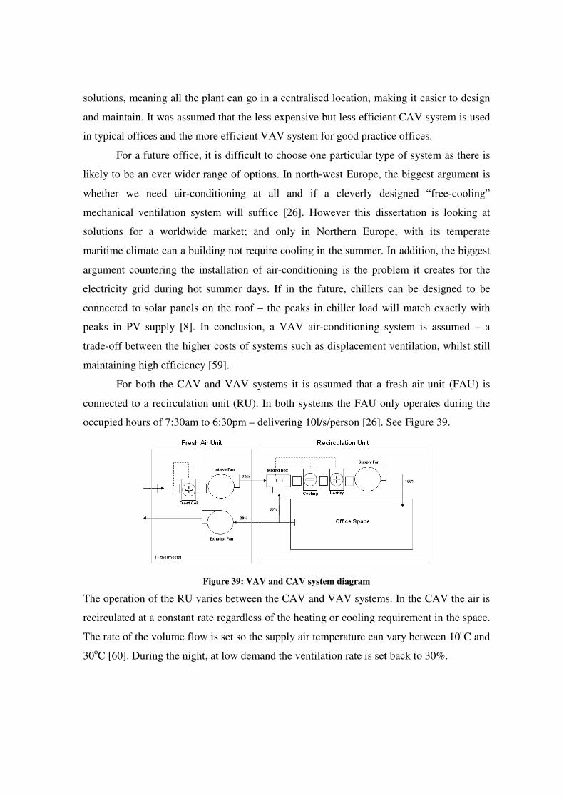
solutions, meaning all the plant can go in a centralised location, making it easier to design

and maintain. It was assumed that the less expensive but less efficient CAV system is used

in typical offices and the more efficient VAV system for good practice offices.

For a future office, it is difficult to choose one particular type of system as there is

likely to be an ever wider range of options. In north-west Europe, the biggest argument is

whether we need air-conditioning at all and if a cleverly designed “free-cooling”

mechanical ventilation system will suffice [26]. However this dissertation is looking at

solutions for a worldwide market; and only in Northern Europe, with its temperate

maritime climate can a building not require cooling in the summer. In addition, the biggest

argument countering the installation of air-conditioning is the problem it creates for the

electricity grid during hot summer days. If in the future, chillers can be designed to be

connected to solar panels on the roof – the peaks in chiller load will match exactly with

peaks in PV supply [8]. In conclusion, a VAV air-conditioning system is assumed – a

trade-off between the higher costs of systems such as displacement ventilation, whilst still

maintaining high efficiency [59].

For both the CAV and VAV systems it is assumed that a fresh air unit (FAU) is

connected to a recirculation unit (RU). In both systems the FAU only operates during the

occupied hours of 7:30am to 6:30pm – delivering 10l/s/person [26]. See Figure 39.

Figure 39: VAV and CAV system diagram

The operation of the RU varies between the CAV and VAV systems. In the CAV the air is

recirculated at a constant rate regardless of the heating or cooling requirement in the space.

The rate of the volume flow is set so the supply air temperature can vary between 10oC and

30oC [60]. During the night, at low demand the ventilation rate is set back to 30%.

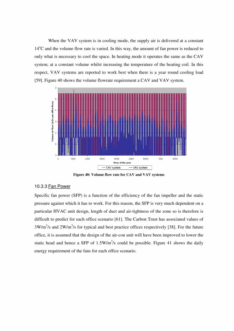
When the VAV system is in cooling mode, the supply air is delivered at a constant

14oC and the volume flow rate is varied. In this way, the amount of fan power is reduced to

only what is necessary to cool the space. In heating mode it operates the same as the CAV

system; at a constant volume whilst increasing the temperature of the heating coil. In this

respect, VAV systems are reported to work best when there is a year round cooling load

[59]. Figure 40 shows the volume flowrate requirement a CAV and VAV system.

Figure 40: Volume flow rate for CAV and VAV systems

10.3.3 Fan Power

Specific fan power (SFP) is a function of the efficiency of the fan impeller and the static

pressure against which it has to work. For this reason, the SFP is very much dependent on a

particular HVAC unit design, length of duct and air-tightness of the zone so is therefore is

difficult to predict for each office scenario [61]. The Carbon Trust has associated values of

3W/m3/s and 2W/m3/s for typical and best practice offices respectively [38]. For the future

office, it is assumed that the design of the air-con unit will have been improved to lower the

static head and hence a SFP of 1.5W/m3/s could be possible. Figure 41 shows the daily

energy requirement of the fans for each office scenario.

0

20

40

60

80

100

120

140

160

1 15 29 43 57 71 85 99 113 127 141 155 169 183 197 211 225 239 253 267 281 295 309 323 337 351 365

Day of the year

Da

ily

Fa

n E

ne

rgy

De

ma

nd

Wh

/m2

Typical

Good Practice

Future

Figure 41: Fan energy requirement comparison between the different office scenarios

10.3.4 Heat Recovery

A good practice way to reduce the heat requirement in cold winter days is to recover the

lost heat when the warm air is exhausted from the building. During occupied hours 20% of

the ventilated air is removed from the building – and using the conventional system, all the

associated heat in this air is lost too. The heat recovery wheel is an air-to-air heat exchanger

transferring the heat from the hot exhaust air to the intake air at a small energy cost. The

newly warmed fresh air component mixes with the rest of the exhaust air in the mixing box,

reducing the amount of reheating required in the recirculation unit. The good practice

office scenario has a heat recovery wheel installed in the fresh air unit, shown in Figure 42.

Figure 42: HVAC system with Heat recovery wheel in the Fresh Air Unit

The heat exchanger is assumed to have a good effectiveness of 80% [64]. Assuming the

same volume flow in the intake and exhaust flows – the performance of the heat exchanger

is given by the following equation:

( )( )11

12

max SE

SS

tt

tt

q

q

−

−==ε Equation 5

Where, ε = effectiveness, q = actual heat transfer and qmax = maximum heat transfer

The future office is assumed to have a hygroscopic thermal wheel – which can

transfer moisture as well as heat. This can reduce the humidification and dehumidification

load to save even more energy. A hygroscopic wheel uses the concept of total effectiveness

which takes into account both latent and sensible heat transfer [64].

SoutinPS

ToutinT

ttmCq

hhmq

ε

ε

)(

)(

−=

−= Equation 6

Where, qT=qS+qL = Total energy transfer (kW), m = mass flow (kg/s), Cp= specific heat =

(1.00kJ/kg.K), tin = dry bulb temperature entering exchanger (oC), tout = dry bulb

temperature leaving exchanger (oC), hin = enthalpy of air entering exchanger (kJ/kg), hout

= enthalpy of air leaving exchanger (kJ/kg), εT = Total Effectiveness, εS = Sensible

Effectiveness.

It is assumed that a total effectiveness of 70% will be possible in the future scenario.

10.3.5 Humidity control

To achieve the humidity setpoint of 50% relative humidity in the summer, the fresh air

input will have to be dehumidified. This is achieved by cooling the air down past its dew-

point temperature and forcing the moisture out of the air. This requires an in-depth controls

analysis into the amount of air which will be cooled down at any given point, including an

analysis of the contact ratio of the coils, airflow speed and coil temperature. As an

approximation, the latent cooling as derived by ESP-r will be used and simply added on to

the total cooling requirement to be met by the chiller.

In the same way, humidification can be achieved in a number of ways including

dew-point wet coil, ultrasonic and steam injection. As a simplification, it is assumed that

the latent heating as derived by ESP-r will approximate this additional heating requirement

by the boiler.

10.3.6 Boiler Performance

Boiler performance is dependent on the part load conditions in which it is operating. The

efficiency at different part load levels are taken from CIBSE guide B [60] for both

conventional and condensing boilers. A further reduction of 20% is taken to account for

pumps and other losses in the system.

40%

50%

60%

70%

80%

90%

100%

0% 25% 50% 75% 100%

Part Load

% e

ffic

ien

cy

Condensing Boiler

Conventional Boiler

Figure 43: Boiler Part-load performance

10.3.7 Chiller Performance

The cooling performance is dependent on part load conditions of the chiller and also

ambient temperature which affects the efficiency of the condenser. The coefficient of

performance (COP) of a chiller with conventional condenser performance is shown in

Figure 44 [63]. It can be seen that at higher ambient temperatures the less effective the

condenser is at exhausting heat and hence gives a lower COP.

0.0

0.5

1.0

1.5

2.0

2.5

3.0

3.5

4.0

20% 30% 40% 50% 60% 70% 80% 90% 100%

Part Load

CO

P

35°C 30°C 25°C 20°C 15°C Figure 44: Conventional chiller system COP

A future scenario is shown in Figure 45, in which the chiller and condenser performance is

maximised in all operating conditions [63]. At lower ambient temperatures, this has a big

impact and the COP can increase to 7 at 70% part load; whilst at 35oC, there is little

difference from the conventional system.

0.0

1.0

2.0

3.0

4.0

5.0

6.0

7.0

8.0

20% 30% 40% 50% 60% 70% 80% 90% 100%

Part Load

CO

P

35°C 30°C 25°C 20°C 15°C Figure 45: Future chiller system COP

Running through an annual simulation, a comparison between the levels of COP reached

by different office scenario chillers is seen below:

Figure 46: COP variation throughout the year for the different office scenarios

11 Total Energy End-use Review

11.1 Auxiliary Loads

11.1.1 Hot Water Energy Consumption

Hot water consumption values have been taken from the ECON-19 office benchmark data

[38].

End-use System type Good Practice Typical

Hand Washing local electric 4 kWh/m2 7 kWh/m

2

Hand Washing central gas boiler 7 kWh/m2 10 kWh/m

2

Hand Washing and catering kitchen

central gas boiler 12 kWh/m2 20 kWh/m

2

Table 18: Hot Water Energy Consumption

11.1.2 Lift Energy Consumption

Lift energy consumption is reported to represent 5% of electrical consumption per year

[66]. Using values extrapolated from a case study by Peters [65], values for typical and

good practice in both high and low-rise buildings can be calculated.

Daily EUI

High-rise Low-rise High-rise Low-rise kWh/day/building kWh/m2/year

Typical 745 112 5 4

Good Practice 459 69 3 2

Future 459 69 3 2

11.1.3 Catering

Catering has been ignored for this study.


An overall energy use index taking into account the 8 loads in the office are presented here.

11.2.1 Typical Office

0

200

400

600

800

1000

1200

1400

1600

1800

2000

1 17 33 49 65 81 97 113 129 145 161 177 193 209 225 241 257 273 289 305 321 337 353

Days of the year

Da

ily

En

erg

y C

on

su

mp

tio

n W

h/m

2

Humidification

Heating

Hot Water

Cooling

Fans

Lighting

IT

Lifts

Figure 47: Typical office annual energy use

11.2.2 Good Practice

0

200

400

600

800

1000

1200

1400

1600

1800

2000

1 17 33 49 65 81 97 113 129 145 161 177 193 209 225 241 257 273 289 305 321 337 353

Days of the year

Da

ily

En

erg

y C

on

su

mp

tio

n W

h/m

2

Humidification

Heating

Hot Water

Cooling

Fans

Lighting

IT

Lifts

Figure 48: Good Practice annual energy use

11.2.3 Future

0

200

400

600

800

1000

1200

1400

1600

1800

2000

1 17 33 49 65 81 97 113 129 145 161 177 193 209 225 241 257 273 289 305 321 337 353

Days of the year

Dail

y E

nerg

y C

on

su

mp

tio

n W

h/m

2

Humidification

Heating

Hot Water

Cooling

Fans

Lighting

IT

Lifts

Figure: Future office annual energy use

11.2.4 Summary

0 50 100 150 200 250 300 350

Typical

Good Practice

Future

Energy Use Index (EUI) kWh/m2

Cooling

Fans

Lighting

IT

Lifts

Hot Water

Heating

Humidification

Figure 49: The three office scenarios annual energy use comparison

11.3 Summary

A future office could have a EUI reduction of 67% from current standard.


EUI

(kWh/m2)

CEI (kgC/m

2)

EUI (kWh/m

2)

CEI (kgC/m

2)

EUI (kWh/m

2)

CEI (kgC/m

2)

Cooling 24 13 28 16 11 6

Fans 41 23 23 13 15 8

Lighting 66 37 34 19 13 7

IT 42 23 30 17 9 5

Lifts 4 2 2 1 2 1

Hot Water 14 3 9 2 9 2

Heating 104 20 40 8 44 9

Humidification 26 5 11 2 3 1

Total 320 127 176 77 105 38

Reduction 0% 0% 45% 39% 67% 70%

11.4 Verification and discussion

The results of the study seem to correlate quite well to those from the carbon trust. In both

the typical and best practice offices – the heating load is underestimated compared with the

Carbon Trust values. This could be from added inefficiencies in perimeter heating systems

and convection current losses.

Key: 1 = naturally ventilated cellular, 2 = naturally ventilated open-plan, 3 = air-

conditioned standard and 4 = air-conditioned prestige

Figure 50: Carbon Trust Econ-19 office energy consumption benchmarks[38]

12 PV Resource

12.1 Overview

Solar energy is the most abundant source of energy in the world. To power the entire UK,

only 1.7% of the country would need to be covered in photovoltaic cells [67]. This can be

compared with figures of 12-15% for wind energy [76]. This is surprising, considering that

the UK is renowned for its windy weather and not its sunshine.

Countries in the south of the EU, such as Spain could generate double the amount

of PV electricity compared with the UK. See Figure 51 for a comparison between the

maximum potential in different EU countries.

Figure 51: Photovoltaic Solar Electricity Potential in European Countries [67]

12.2 Photovoltaic Panels and Efficiency

PV panels traditionally convert sunlight into electricity by harnessing the effect that

the photons have on bumping electrons across a doped silicon layer. When this can be

achieved on a mass scale (hence the large flat surface) an electric current is formed [75]. To

date this has occurred at a massive efficiency cost – and the best commercially available

crystalline-Si cells only convert a maximum of 13% of the available solar radiation. The

first assumption to challenge is that future PV technology will remain in the same

condition.

In a paper analysing the policy of the R&D and deployment of PV, 18 experts in the

field were asked their opinion on the cost and efficiency of the PV in the future [68]. As PV

does not cover just one type of technology but a family of concepts, the first big question

is: is there a clear favourite technology choice that we want to adopt? The answer was

unanimously no, and that the current approach of designing a multitude of concepts, with

no biases on the different maturity level of each technology is valuable to the progress of

the industry.

Estimations of efficiencies for the year 2030 varied wildly even in within one PV

type. The table below catalogues the key predictions from the paper; whilst mature

technology such as Crystalline-silicon could only achieve a high best efficiency of 25% by

2030, “novel, high-efficiency” technology such as the hot carrier, plasmonics or

thermophotovoltaic concepts could achieve a high-best efficiency of 45%.

Extremes in estimated efficiencies (2030)

Technology*Crystalline-

Si

Thin film

2a+b

Thin film

2c+d

Thin film

2d+e+

composite

Concentrator ExcitonicNovel, high-

efficiency

high max. value (%) 30 35 29 30 65 25 52

high best estimate (%) 25 30 24 25 53 19 45

low best estimate (%) 14 10 10 13 25 7 14

low min . value (%) 13 7 8 9 20 3 8 Table 19: Summary of expected PV efficiencies in 2030 [68]

It is clear from this information it would be difficult to associate a single value of

efficiency for PV technology available in 10 years time. However, PV efficiency was

needed to be set to run the simulations, so a value of 20% was chosen. Falling between

most high and low best estimates for 2030, it was deemed neither too conservative nor

overly optimistic.

12.3 Geometry of Building and PV Panels

The amount of solar power generated by a building depends on three geometric

considerations; how many of the surfaces of the building are covered in PV, how much of

each surface is covered and what tilt angle the panel is at.

Solar radiation is made up of two components: direct and diffuse light. Direct beam

comes directly from the sun, whilst diffuse radiation as the name suggests is diffused on

something first – such as a cloud. Diffuse radiation is always present even if it is not

noticed because of the larger presence of direct sunlight (except on overcast days when

100% of light it diffuse). Solar panels are normally never positioned on the north side of

the building (in the northern hemisphere) as it would see very little or no sun all year round

and would make little sense as an investment.

Figure 52: Direct and Diffuse solar radiation components for London

The angle that the PV panel makes with the sun is an important factor to how much

energy can be delivered to the panel in a year. It has been assumed in this study that the

façade panels are fixed vertically to the walls (South, West and East façades only). The

complex relationship between PV tilt angle, and the shading effect on the winds (which

effects lighting and cooling loads) requires further analysis outside the scope of this thesis.

The roof panels are assumed to be facing south and the tilt angle can be varied. This

optimal tilt angle is a function of many different parameters including the latitude of the

site (macro-climate effects), cloud cover patterns (micro-climate effects) and local shading

effects.

The energy modelling software ESP-r created by the university of Strathclyde has

an inbuilt function to calculate the PV energy generation of any surface. However, to

calculate the optimum tilt angle meant that 10 different models would required for every

location (ultimately 60 simulations in total). A more efficient approach was to model the

interaction from the sun and panels from equations derived from first principles. An Excel

spreadsheet was created where it was much more straightforward to manipulate the tilt

angle and hence the maximum possible PV generation could be found for each location.

12.4 Optimum Tilt angle from first principles

Weather stations record the data on the average diffuse and direct beam components

of solar radiation for every hour of the year and the US department of Energy has a

directory of data files for locations all over the world [50].

The diffuse component is only dependent on the amount of sky that the panel can

“see”, and therefore is dependent only on the tilt angle of the panel. The direct component

varies during the day depending on the angle that the direct beam makes on the panel –

which is always changing depending on the time of day and year, the location and the

orientation and tilt of the collector. Formulas for calculating the various solar angles are

well defined and can be found in numerous sources [70, 71, 72, 73, 74]. Due to the large

number of variables involved, there does not seem to be a consistent range of mathematical

symbols between the different sources. To avoid confusion, a list of the mathematical

symbols for each variable is listed in the table below:

Altitude β

Solar azimuth angle γs

Incident angle θ

The surface azimuth angle γ

The surface solar azimuth angle α

The tilt angle (measured from horizontal) Φ

Declination δ

Hour Angle h

Latitude ζ

Masking angle ψ Table 20: Symbols used in solar angle calculations

12.4.1 Modelling the Sun

The path of the sun can be tracked using only the angles of altitude and azimuth.

Solar Altitude, ( )δζδζβ sinsincos)cos(cossin 1 += − h Equation 7

Solar azimuth,

−= −

β

δζδζγ

cos

sincoscos)cos(sincos 1 h

s Equation 8

Figure 53: Explanation of solar azimuth and elevation [75]

These two solar angles are dependent on three factors (δ, h and l) which are specific to each

location and time on earth.

• Declination: (δ) the variability of the seasonal angle from the 23.5o declination angle from the earth/sun normal orbit.

+××=

365

)284(360sin0

nδδ , where δo =23.5

o and n = day of the year Equation 9

• Hour Angle: (h) converts the sun path “time” into angular notation. Dependent on the real solar time: which differs from the unadjusted reference time around the world, by taking into account extra correction factors which characterise the earth’s annual revolution patterns.

Where )12(15 solth −= [am] and )12(15 −= solth [pm] Equation 10

And

+−+=

60

)(4 ELLtt

ref

refsol Equation 11

Where L = longitude of site (London = -0.18o), Lref=Longitudinal reference (UK is 0

o)

And βββ sin5.1cos35.7)2sin(87.9 −−=E and 364

)81(360 −=

nB Equation 12

• Latitude: (ζ) the distance the site is from the equator: London is 51.51o N.

12.4.2 Direct Radiation on Horizontal and Vertical Surfaces

The component of the measured direct beam falling on a horizontal surface is:

βsinbbH II = Equation 13

The component of the measured direct beam falling on a vertical surface is:

αβ coscosbbV II = Equation 14

α = wall solar azimuth (which is adjusted to take into account the orientation of the wall relative to

south; α = γ- γs. As the wall is south facing, γ=0 and α = - γs (-solar azimuth angle))

12.4.3 Direct Radiation on Tilted Panels

The direct component received by a tilted panel is calculated by combining the horizontal

and vertical vectors shown in equations 1 and 2.

)cossinsincos(cos Φ+Φ=Φ βαβbb II Equation 15

Φ= tilt angle, measured from horizontal.

Where IbΦ ≥ 0 for non-negative values of both expressions in the parenthesis, otherwise IbΦ=

0.

12.4.4 Diffuse Radiation

The diffuse radiation is calculated as a fraction of the hemisphere the panel can “see”. A

flat panel without any obstruction will see the entire amount as recorded in the weather file.

As the plate is tilted, the fraction seen is decreased, as shown in the diagram below.

Figure 54: North-south section explaining diffuse radiation on tilted panels

Diffuse radiation on a tilted panel on the roof:

Φ+=Φ 2

cos1dhd II Equation 16

A panel placed vertically on the wall will only “see” half of the hemisphere, so this

equation is simplified to:

=Φ 2

1dhd II Equation 17

12.5 Optimum tilt for panels with local shading

The equations for the direct and diffuse components are only valid if there is only one PV

panel per surface. In reality, the PV panels will likely be organised in rows, in which by

increasing the tilt of each panel increases the shading on the adjacent panel. This will

reduce the effectiveness of the panels at greater tilt angles, and produce a more realistic

maximum PV resource for each surface. As seen in the figure below, the rooftop shading is

most evident at low sun angles – early morning or evening. As discussed before, the wall

based panels are assumed to be fixed vertically to the wall and are not included in this

analysis.

Figure 55: Shading occurring on rooftop PV panels

12.5.1 Direct Beam Shading Coefficient

Using first principles, this requires finding a diffuse and direct beam shading coefficient for

the different panel configurations. J. Appelbaum et al 1979 [73] and D. Passias et al 1983

[72] have shown that the direct beam shading coefficient (CSD) as a % of the total panel

area is:

+

×−×

+

×−=L

ADh

A

ADCSD

φ

θ

δφφ

θ

β cos

cos

)sin(cossin1

cos

cos

sin1 Equation 18

Where, β = solar altitude as defined above, and θ = incidence angle. For a south facing

panel,

( ) ( ) )cos(coscossinsincos hδφζδφζθ −+−= Equation 19

Where the parameters refer to Figure 56:

Figure 56: Direct beam shading from adjacent panels (from Appelbaum et al. [73])

The shaded direct beam (IBS) is then calculated from:

SDBBS CII = Equation 20

12.5.2 Diffuse Shading Coefficient

In the same way, shading from the adjacent panel will reduce how much a panel can “see”

the hemisphere. The adjacent panel causes a “masking effect” and will reduce the total

level of diffuse irradiance hitting the surface. This is particularly important in climates

where diffuse radiation is predominant. The level of this “masking effect” is defined by the

masking angle ψ and depends on the position along the surface (z) of panel – as is shown in

Figure 57 [72].

Figure 57: Diffuse beam shading impact from adjacent panels (from Passias et al. [72])

Where ( )

+−

−=

φφ

φψ

coscos

sinarctan)(

zAC

zAz Equation 21

To find the overall diffuse shading coefficient, it is necessary to find the average masking

angle, with respect to z:

∫=A

dzzA 0

)(1

ψψ Equation 22

This average masking angle varies depending on the inclination of the panel, and on the

closeness of the adjacent panel. With k = C/A = 1, (adjacent panel one panel length away),

the maximum masking angle is 32o and with k = 3 (adjacent panel three panel lengths

away), the maximum masking angle is under 10o. These results correspond with the study

done by D. Passias et al [72].

0

5

10

15

20

25

30

35

0 10 20 30 40 50 60 70 80 90

Inclination Angle (degrees)

Avera

ge m

askin

g a

ng

le (

deg

rees)

k = 1

k = 1.5

k = 3

Figure 58: Average masking angles vs. inclination angle for various values of C/A (=k)

Overall diffuse irradiance is recalculated taking into account this average masking angle:

−

+

= 1

2cos

2cos 22 ψφ

DDS II Equation 23

12.5.3 Verification with ESP-r

The panels are assumed to be in rows across the entire width of the speculative building

(45m), and assuming PV panels of 1.5m in length means 30 rows of panels can fit on the

roof.

Verification study

• row width (L) = 45m • panel length (A) = 1.5m, • tilt angle of 30o and facing south

Figure 59: Roof PV layout

As seen in Figure 60 and Figure 61, there is a close correlation between the monthly direct

beam shading coefficients between the ESP-r model and excel spreadsheet. The excel sheet

tends to slightly underestimate the shading coefficients during the summer, but overall the

shape and magnitude is the same.

0%

10%

20%

30%

40%

50%

60%

70%

80%

90%

100%

00:00 03:00 06:00 09:00 12:00 15:00 18:00 21:00 00:00

Sh

ad

ing

Co

eff

icie

nt

(%)

Jan

Feb

March

April

May

June

July

August

Sept

Oct

Nov

Dec

Figure 60: Monthly direct beam shading coefficients using Excel

0%

10%

20%

30%

40%

50%

60%

70%

80%

90%

100%

00:00 03:00 06:00 09:00 12:00 15:00 18:00 21:00 00:00

Sh

ad

ing

Co

eff

icie

nt

(%)

Jan

Feb

March

April

May

June

July

August

Sept

Oct

Nov

Dec

Figure 61: Monthly direct beam shading coefficients using ESP-r

Using the climate data for Gatwick Airport, the energy generated from the Excel and ESP-r

models were compared.

0

200

400

600

800

1000

1200

1400

1600

1 31 61 91 121 151 181 211 241 271 301 331 361

Days of the year

To

tal

Da

ily

En

erg

y W

h/m

2

Excel Method

ESPr Simulation

Figure 62: PV generation comparison between ESP-r and Excel for a London climate

Overall there is a very good correlation. There seems to be a slight unexplainable disparity

in the months of April and August and in the summer the model tends to slightly

underestimate the peaks in PV generation; perhaps explained with the small discrepancy

between the direct beam shading coefficients.

Energy Delivered kWh/m2

Excel ESPr % Difference

1st Quarter 22.6 22.6 0.0%

2nd Quarter 73.1 73.3 -0.2%

3rd Quarter 67.7 66.6 1.5%

4th Quarter 16.6 16.5 0.6%

Annual Total 179.9 179.0 0.5%

Table 21: PV generation comparison between ESP-r and Excel for a London climate

12.6 Optimum Tilt Angle

Some interesting conclusions were found: whilst the optimum angle for an unshaded PV

panel in London is around 30o from horizontal; when the panels are arranged in south

facing rows along the roof, the shading affect from the adjacent panel means that the

optimum position is actually horizontal.

The slight increase in shading from tilting the panel immediately cancels off any

benefit from tilting the panel towards the sun. The global irradiation for different tilt angles

is shown in Figure 63; which can be seen to correlate with the values predicted by Šúri et

al. [67] in their solar map of Europe.

0

200

400

600

800

1000

1200

0 10 20 30 40 50 60 70 80 90

Tilt Angle (degrees)

Glo

bal

Irra

dia

tio

n (

kW

h/m

2)

Unshaded Shaded

Figure 63: Global irradiation for panels at different tilt angles in London

13 International Case Studies

13.1 Rationale for choosing location

In this dissertation a number of locations have been simulated to discover the potential

opportunities and drawbacks of different climates. The challenge was to choose a sample

range of cities that balances the following three criteria:

• Are seen as hotspots for trade and commerce

• Represent a wide range of climatic conditions

13.1.1 Worldwide Trade and Commerce

The first criterion was examined using the MasterCard Worldwide Centers of Commerce

Index 2008 [78]. The Index is a list of the top 75 cities in the world to do commerce in. It

ranks each city based on 7 different criteria; appraising their legal and political framework,

the economic stability, ease of doing business, financial flow, business centre, knowledge

creation and information flow and finally livability.

From the pie chart, it can be seen that the majority of the split is between Europe,

Asia and North America, with little impact from Latin America.

North America

19%

Latin America

9%

Asia/Pacific,

Middle East and

Africa

35%

Europe

37%

Top 10 Cities

Rank City Country Region

1 London UK Europe

2 New York United States North America

3 Tokyo Japan Asia/Pacif ic

4 Singapore Singapore Asia/Pacif ic

5 Chicago United States North America

6 Hong Kong Hong Kong Asia/Pacif ic

7 Paris France Europe

8 Frankfurt Germany Europe

9 Seoul South Korea Asia/Pacif ic

10 Amsterdam Netherlands Europe

Figure 64: MasterCard Centers of Commerce:

Continental split

Table 22: MasterCard Centers of Commerce:

Top ten cities

In the top 10 places there are 4 European cities, 4 Asian cities and 2 North American cities.

However, these 10 do not entirely represent the wide range of climate conditions in the

world – especially because of the vicinity of the European countries to each other.

13.1.2 Worldwide Climate zones

The Köppen climate classification is the most widely respected system for dividing the

world into discreet zones of similar climate [79]. It was developed by Wladimir Köppen

around 1900, and categorises the world into different climate zones through vegetation

distribution, temperature, precipitation and the seasonality of the precipitation [80, 81].

Global climate is divided into 5 classes and then subdivided further into different groups.

Figure 65: World map of the Köppen-Geiger climate classification [81]

• Class A: Tropical Climate (Subclasses: Equatorial, Monsoon and Savanna)

o Tropical climates are defined as having a constant high temperature above

18oC throughout the year and large annual rainfall.

o Equatorial climates are found between 5-10o of the equator and whilst there

are no real seasons, rainfall of at least 60mm is expected every month.

o Monsoon climates are found adjacent to the equatorial climates, which with

the seasonal winds (especially in South-east Asia) means there is a distinct

wet and dry season.

• Class B: Dry (Subclasses: Desert and Semi-arid)

o Desert regions are defined as receiving less than 250mm precipitation per

year, whilst semi-arid is between 250-500mm. The lack of cloud cover

means there is a lot of solar energy available during the day, but also

extreme cooling requirements.

• Class C: Temperate (Subclasses: Humid Subtropical, Maritime, Mediterranean)

o Mediterranean climates are found on western coasts between 30-45o of

latitude; in winter they have changeable and rainy weather but have hot and

dry summers.

o Maritime climates are also found on western coasts, immediately poleward

of Mediterranean climates and reaching as far 60o in Western Europe. The

weather is dominated by polar fronts giving changeable and overcast

weather all year round. Summers are cool because of cloud cover and

winters are mild compared with similar latitudes.

o Humid subtropical weather occurs on eastern coasts from 25-40o of latitude;

unlike Mediterranean weather, the summers are humid and wet.

• Class D: Continental (Subclasses: Humid Continental, Subarctic and Continental

Mediterranean)

o Found in the interior of continents where the average summer temperature is

above 10oC and winter averages above -3oC. There is often a conflict

between polar and tropical air masses and hence huge seasonal variability.

• Class E: Polar (Subclasses: Polar and Alpine)

o Defined as areas where the temperature is below 10oC average all year.

There are no major cities in this climate and is therefore not considered.

13.2 Selecting the Sample Range

It was decided that a sample size of 6 was possible to cover the most important climate

zones: including – Equatorial (Tropical), Desert (Dry), Humid Subtropical, Maritime and

Mediterranean (Temperate) and Humid Continental (Continental). To help in the decision

process, a table was created to compare the choices of the cities found in each zone, their

latitude and longitude and their MasterCard ranking.

6 sample cities

Class Name Subclasses Symbol Cities Latitude Longtitude

Mastercard

City Rating

A Tropical Equatorial Af Singapore 1.23 103.92 4

Kuala Lumpur 3.13 101.70 50

Monsoon Am Mumbai 18.98 72.83 48

Miami 25.79 -80.22

Rio de Janeiro -22.90 -43.23 65

Savanna Aw,As Bangalore 12.97 77.57 66

B Dry Desert BWh,BW k Dubai 25.20 55.30 44

Semi-arid BSh,BSk Denver 39.74 -104.98

C Temperate Humid subtropical Cfa, Cwa Shanghai 31.20 121.50 24

Hong Kong 22.30 114.20 6

Tokyo 35.68 139.77 3

Houston 29.76 -95.38 34

New York 40.72 -74.00 2

Milan 45.46 9.19 20

Marit ime Cfb,Cwb,Cfc London 51.51 -0.13 1

Frankfurt 50.11 8.68 8

Amsterdam 52.37 4.89 10

Dublin 53.35 -6.26 31

Mediterranean Csa,Csb Barcelona 41.38 2.18 38

Rome 41.90 12.50 47

Los Angeles 34.05 -118.25 17

San Francisco 37.78 -122.42 28

D Continental Humid continental Dfa,Dwa,Dfb,Dwb Toronto 43.67 -79.38 13

Chicago 41.89 -87.62 5

Beijing 39.90 116.40 57

Seoul 37.55 126.98 9

Subartic Dfc,Dwc,Dfd,Dwd

Continental MediterraneanDsa,Dsb,Dsc Madrid 40.40 -3.68 11

E Polar Polar ET,EFAlpine ET/H

Table 23: Comparison between the climates of world cities

The 6 final cities chosen were: Singapore, Chicago, Hong Kong, London, Los Angeles and

Dubai. The first four are in the top ten ranking, whilst the remaining two are 17th and 44th

respectively. Although the highest MasterCard rankings were not always chosen, the

sample provided the largest variation in latitudes of the possible choices.

13.3 Building Scenarios

13.3.1 Scenario 1: Sheltered urban low-rise

Central London is a good example of a densely urbanised, low-rise environment. Using

data from the IKONOS-2 satellite; it can be seen in Figure 66 that most of the buildings,

which are shown in dark blue or pink, vary between 16 and 26 metres.

Figure 66: Building Height in Central London

using IKONOS data [77]

Figure 67: Fitzroy Street in London shading from

trees and adjacent buildings [82]

Scenario 1 is loosely based on Arup’s new Fitzrovia office, shown in Figure 67 (above);

assumed to be in a dense urban area with shading from trees and adjacent buildings. With

these high levels of shading throughout the day, PV generation is only possible on the roof,

as shown in the models below.

Building Dimensions

Length x width 45m x 45m Floor to ceiling height 2.7m

Ceiling void 1.4m Total height 25m

Floors 6 Floor area per level 1800m2

Total office floor area 10800m2

PV Dimensions Number of panels on roof 1350

Total PV area 2025m2

Figure 68: Details of urban low-rise scenario

13.3.2 Scenario 2: Semi-exposed downtown high-rise

The second scenario is a semi-exposed high-rise building in the downtown area of a city.

Figure 69: View of Toronto downtown area

As can be seen in the typically dense downtown skyline of Toronto, most high-rise

buildings are neither fully exposed, nor fully sheltered but have at least 1 side uncovered.

Hence, it is assumed PV generation is possible on the south, east and west façades of the

top half of the building.

Building Dimensions

Length x width 45m x 45m Floor to ceiling height 2.7m

Ceiling void 1.4m Total height 140m

Floors 32 Floor area per level 1800m2

Total office floor area 57600m2 PV Dimensions

Number of panels on roof 1350 Number of panels on façade 2025

Total number of panels 3375 Total PV area 5078m2

Figure 70: Downtown High-rise scenario details

13.4 PV Generation Potential

13.4.1 Optimal Tilt Angle

The optimum tilt angle for shaded and unshaded PV panels positioned on the roof of the

building were compared in the 6 worldwide locations.

0

500

1000

1500

2000

2500

0 10 20 30 40 50 60 70 80 90

Tilt Angle from Horizontal

En

erg

y D

en

sit

y k

Wh

/m2

0

500

1000

1500

2000

2500

0 10 20 30 40 50 60 70 80 90

Tilt Angle from Horizontal

En

erg

y D

en

sit

y k

Wh

/m2

Figure 71: Global irradiation for shaded panels in

different world locations

Figure 72: Global irradiation for unshaded panels

in different world locations

As expected in the unshaded PV panels – the optimum tilt is most heavily influenced by the

latitude at which the site is at. The closer the site to the equator the higher the altitude of

the sun at midday – which means a tilt angle closer to horizontal, is desired.

There are some surprising results when shading effects are included – the optimum

level is horizontal irrespective of the latitude or climate of the site.

Optimal PV Tilt Angle

Latitude Unshaded Shaded

London 51.51° 28° 0° Chicago 41.89° 28° 0°

LA 34.05° 27° 0° Dubai 25.2° 24° 0°

Hong Kong 22.3° 14° 0° Singapore 1.23° 0° 0°

Table 24: Optimal PV tilt angle in different worldwide locations

Shading effects from adjacent terrain, including other buildings, trees and nearby hills have

not been included in this analysis. However it is clear from this study that shading is a

major influence on the global irradiance potential of a particular site – and a thorough, site-

specific study is required at the design stage.

13.4.2 PV Generation per building type

A key difference between the low-rise and high-rise scenarios is with the PV generation

opportunity.

Low Rise High Rise

PV area on walls (m2) 0 3053

PV area on roof (m2) 2025 2025

Total PV area (m2) 2025 5078

Gross Floor area (GFA) (m2) 10800 57600

PV panel area : GFA ≈ 1:5 ≈ 1:11

Table 25: PV opportunity per building type

High rise buildings have a high energy density, with a poor surface area to floor area ratio –

unsuitable for renewable generation. This can be seen in Figure 73; a comparison between

the different worldwide locations.

0

10

20

30

40

50

60

70

80

90

London Chicago Hong Kong Singapore Los Angeles Dubai

PV

gen

era

tio

n o

pp

ort

un

ity

(kW

h/m

2 f

a)

High-rise Low-rise

Figure 73: PV Generation opportunity for different building types around the world

13.5 Energy Demand Comparison

13.5.1 Lighting

Using the same statistical analysis of external diffuse illuminance – the 85% exceedance, or

“design sky” can be compared in the different locations. It can be seen in Figure 74 that the

design sky varies considerably between the locations – up to around 20klux on the equator

– four times greater than in the UK.

0%

10%

20%

30%

40%

50%

60%

70%

80%

90%

100%

0 10 20 30 40 50 60 70 80

Diffuse Illuminance (klux)

% e

xce

ed

an

ce

85% exceedance

London (51° N)

Chicago (42° N)

LA (34° N)

Dubai (25° N)

Hong Kong (22° N)

Singapore (1° N)

Figure 74: External Diffuse Illuminance availability around the world

The associated energy load for lighting is calculated for a future office scenario – with LED

lighting, and same assumptions and procedure as defined in section 9.3.

0

0.2

0.4

0.6

0.8

1

1.2

1.4

1.6

1.8


Mo

nth

ly L

igh

tin

g D

em

an

d k

Wh

/m2

London Chicago LA Dubai Hong Kong Singapore Figure 75: Monthly lighting energy demand comparison around the world

The amount of electric light required varies proportionally to the latitude of the site – with

locations on the equator having the least energy consumption.

Latitude Electric Light

Usage

Total Energy

Demand (kWh/m2)

London 51.5o 65% 13.5 Chicago 41.89o 60% 12.4

Los Angeles 34.05o 58% 11.9 Dubai 25.2o 53% 10.9

Hong Kong 22.3o 52% 10.7 Singapore 1.23o 47% 9.8

Table 26: Summary of electric lighting requirement around the world

13.5.2 Demand Summary

A comparison between the energy demand of both building scenarios – broken down into

the heating and electrical components are shown in Figure 76 and Figure 77.

0

20

40

60

80

100

120

London Chicago Los Angeles Hong Kong Dubai Singapore

Ele

ctr

ical E

nerg

y U

se In

dex

(E

UI)

kW

h/m

2

High-rise

Low-rise

Figure 76: Electrical Demand per building type in each location

0

20

40

60

80

100

120

London Chicago Los Angeles Hong Kong Dubai Singapore

He

ati

ng

En

erg

y U

se In

dex (

EU

I) k

Wh

/m2

High-rise

Low-rise

Figure 77: Heating Demand per building type in each location

Overall, there is not a significant difference in the minimum level of demand each scenario

could potentially reach. Whilst in practice, bigger offices use more energy because they are

harder to design well and the operation cannot be as closely controlled. The energy use

index for both scenarios can be further broken down into the 8 main energy end uses:

cooling, fans, lighting, IT equipment, lifts, hot water, heating and humidification.

0 20 40 60 80 100 120 140 160

London

Chicago

Los Angeles

Hong Kong

Dubai

Singapore


Cooling

Fans

Lighting

IT

Lifts

Hot Water

Heating

Humidification

Figure 78: High-rise Energy Use Index for each worldwide location

0 20 40 60 80 100 120 140 160

London

Chicago

Los Angeles

Hong Kong

Dubai

Singapore


Cooling

Fans

Lighting

IT

Lifts

Hot Water

Heating

Humidification

Figure 79: Low-rise Energy Use Index for each worldwide location

As expected, there is a greater cooling and lesser heating load in the high-rise building as it

is more exposed. The individual daily demand profiles for each city, broken down into each

end use can be viewed in the Appendix 17.2.

13.6 Supply and Demand Matching

The variable nature of renewable energy requires an analysis of the suitability of how the

supply matches with the demands of the building. For example, in high latitudes the PV

resource is very large during the summer but almost non-existent during the winter. This

would match very well with the cooling demands of the building, which are also high in the

summer and low in winter; but not very well with lighting demand which peaks in the

winter.

There are also the supply and matching variations throughout a 24hour period.

Whilst some loads, such as the HVAC or lighting loads could be in operation at night-time,

solar energy is only available during office hours.

13.6.1 Battery Storage Assumptions

In order to use the solar energy received in the summer for lighting in the winter an

impossibly large number of batteries would be required. A way round this is to think of the

national electricity grid as like a battery. Electricity can be sold to the grid during peak

times, and bought back when required.

Ideally, the future low powered office will only require selling and buying

electricity from the grid when it really needs to – so that most of the electricity generated

onsite can be used locally. This requires a trade-off between the two extremes of a strong

grid connection with no battery storage and no grid connection with infinite battery storage.

As a simplification of a detailed analysis into the optimum level of batteries (which would

have to take into account the capital cost of batteries and transformers and potential grid

electricity costs in the future), it is assumed that up to 24hours storage is possible onsite.

Whilst quite optimistic by today’s standards – energy storage technology is constantly

improving [83], and as it has been made quite clear in this dissertation, there are

opportunities in considerably reducing the demand typical and even good practice offices.

13.6.2 CHP analysis

Instead of using a traditional boiler to cover the hot water and heating requirements, a

combined heat and power (CHP) unit could be employed. CHP units generate electricity

locally and so can make use of the waste heat which is normally lost in conventional power

stations [86].

Whilst they can run at over 90% efficiency, they are also more expensive than

boilers, so cost effectiveness depends on how much of year they are needed to operate.

Often they are designed to cover the baseload of heat throughout the year, and coupled with

boilers which can be operated to cover the peak loads in winter. An industry rule of thumb

is that they should be sized to run for around 5000hours per year [85].

13.6.2.1 CHP for hot water

Assuming that in the future, the hot water load will not change from good practice

levels today; it can be seen in Figure 79 that hot water could account for almost 15% of the

annual energy consumption in an office. As this is a heating load which will be ran

throughout the entire working year (6258 hours/year); this is a good candidate for a

dedicated CHP system. The hot water CHP unit chosen for the two buildings are

summarised in the table below.

Scenario Daily hot water

consumption

Average power

(running 24h)

CHP model

[84]

Heat :

Power Ratio

Low-rise 356 kWh/day 14.9kW ENER·G 10y 1.7:1

High-rise 1901 kWh/day 79kW ENER·G 50M 1.5:1

Table 27: CHP for Hot Water summary

It is assumed that a hot water tank would smooth out the hot water supply and demand

variations throughout each working day.

13.6.2.2 CHP for heating

Both London and Chicago have large space heating requirements in the winter, so are

investigated for suitability for CHP. Shown in Figure 80 is the number of running hours per

year for different CHP system sizes.

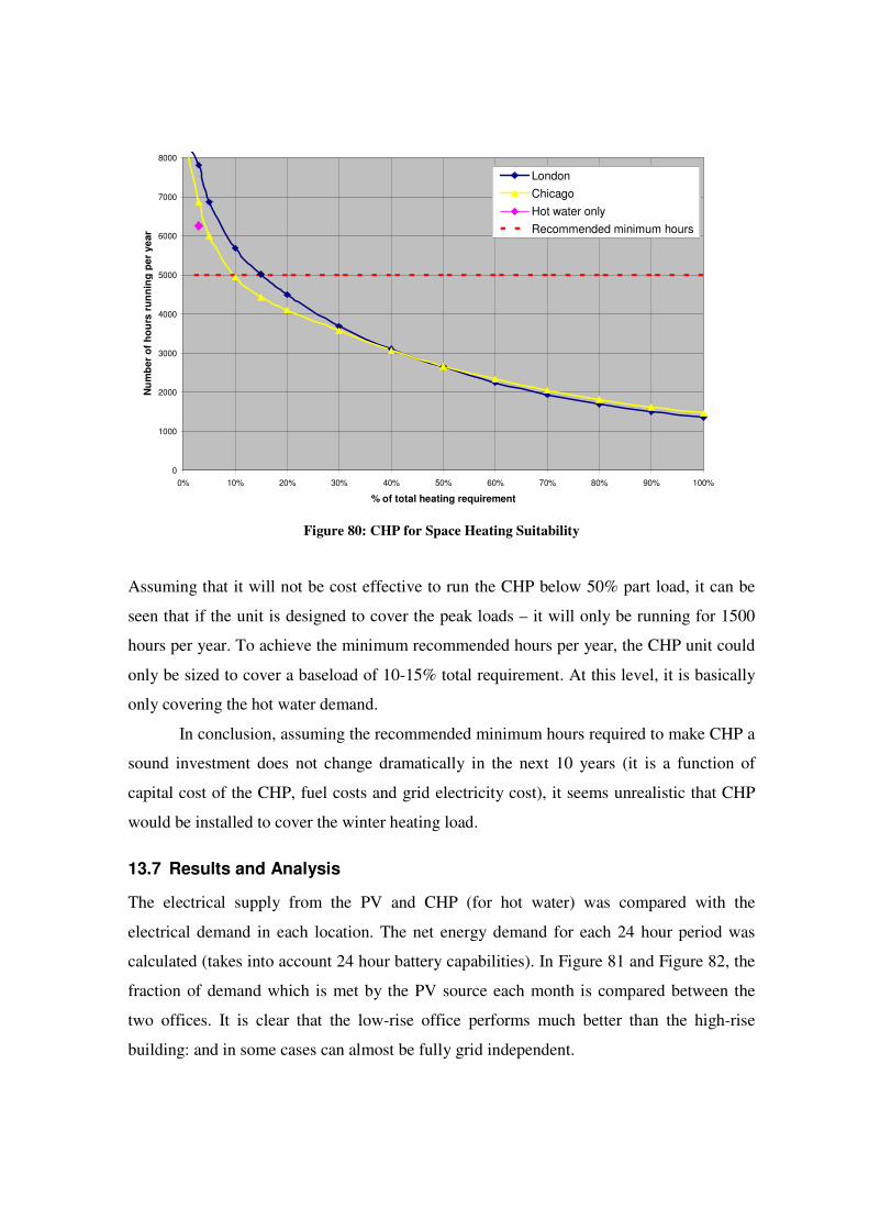
0

1000

2000

3000

4000

5000

6000

7000

8000

0% 10% 20% 30% 40% 50% 60% 70% 80% 90% 100%

% of total heating requirement

Nu

mb

er

of

ho

urs

ru

nn

ing

pe

r y

ea

r

London

Chicago

Hot water only

Recommended minimum hours

Figure 80: CHP for Space Heating Suitability

Assuming that it will not be cost effective to run the CHP below 50% part load, it can be

seen that if the unit is designed to cover the peak loads – it will only be running for 1500

hours per year. To achieve the minimum recommended hours per year, the CHP unit could

only be sized to cover a baseload of 10-15% total requirement. At this level, it is basically

only covering the hot water demand.

In conclusion, assuming the recommended minimum hours required to make CHP a

sound investment does not change dramatically in the next 10 years (it is a function of

capital cost of the CHP, fuel costs and grid electricity cost), it seems unrealistic that CHP

would be installed to cover the winter heating load.


The electrical supply from the PV and CHP (for hot water) was compared with the

electrical demand in each location. The net energy demand for each 24 hour period was

calculated (takes into account 24 hour battery capabilities). In Figure 81 and Figure 82, the

fraction of demand which is met by the PV source each month is compared between the

two offices. It is clear that the low-rise office performs much better than the high-rise

building: and in some cases can almost be fully grid independent.

13.7.1 % of met demand with PV supply

0%

10%

20%

30%

40%

50%

60%

70%

80%

90%

100%


% o

f e

lec

tric

al

de

ma

nd

me

t w

ith

PV

su

pp

ly p

er

mo

nth

London Chicago Los Angeles Dubai Hong Kong Singapore

Figure 81: Low rise Building: % of electrical demand met with PV supply per month

0%

10%

20%

30%

40%

50%

60%

70%

80%

90%

100%


% o

f e

lec

tric

al

de

ma

nd

me

t w

ith

PV

su

pp

ly p

er

mo

nth

London Chicago La Dubai Hong Kong Singapore

Figure 82: High rise Building: % of electrical demand met with PV supply per month

13.7.2 Average electrical demand met by Renewable Source

The average annual demand which is met by these renewable sources gives an indication of

the relative performance of each location. In Figure 83, it is can be seen that Dubai – with

the desert climate performs the best, whilst Los Angeles with the Mediterranean climate is

second best. As expected, the UK with its cloudy skies is the worst performer.

0%

10%

20%

30%

40%

50%

60%

70%

80%

90%

100%


% o

f e

lec

tric

al

de

ma

nd

me

t b

y P

V (

av

era

ge

pe

r y

ea

r)

High-rise

Low-rise

Figure 83: Electrical demand met by PV supply (alone) per year

0%

10%

20%

30%

40%

50%

60%

70%

80%

90%

100%


% o

f e

lec

tric

al

de

ma

nd

me

t b

y P

V a

nd

CH

P

High-rise

Low-rise

Figure 84: Electrical demand met by PV and CHP per year

13.7.3 Excess sold back to the grid

A second metric of performance is to compare how much electricity is surplus per year –

i.e. when the total daily PV supply exceeds the demand. Again, Dubai and LA are the best

performers. As expected, high-rise buildings in all the locations do not have much

opportunity to sell back electricity to the grid.

0

5

10

15

20

25

30

London Chicago Hong Kong Singapore La Dubai

Ele

ctr

icit

y s

old

ba

ck

to

th

e g

rid

(k

Wh

/m2

)

High-rise

Low-rise

Figure: Excess electricity sold back to the grid

13.8 Sensitivities

The high number of different parameters required to undertake this analysis means it is

important to ascertain which of the parameters are highly sensitive to result of the study.

The three parameters which are dependent on location are:

• Lighting (sensitivity: efficacy of future LED lamps)

• Cooling (sensitivity: performance of future chillers)

• Solar energy (sensitivity: efficiency of future PV panels)

13.8.1 Sensitivity 1: LED Efficacy

LED lamps are estimated to be able to achieve an efficacy of 150lumens/W in the next

decade [40]. This study looks into the impact if 100lumens/W is only realistic on a

commercial scale.

0 20 40 60 80 100 120 140 160 180

London

Chicago

Los Angeles

Hong Kong

Dubai

Singapore


Cooling

Fans

Lighting

IT

Lifts

Hot Water

Heating

Humidification

The increase in lighting energy is slightly more apparent in northern locations, but overall it

does not dramatically change the relative shape of the EUI.

0%

10%

20%

30%

40%

50%

60%

70%

80%

90%

100%


% o

f e

lectr

ica

l d

em

an

d m

et

by

PV

an

d C

HP

LED - 150lumens/W

LED - 100lumens/W

There is only a slight decrease in the level of electrical demand which can be met per day,

and not much difference between locations.

13.8.2 Sensitivity 2: Chiller Performance

An important assumption is that in the future, the chiller and condenser technology will be

able to perform much nearer to optimum conditions and temperature set points. This

sensitivity study looks into the impact if the current scenario COP for cooling cannot be

improved on in the future (see section 10.3.7 for more details).

0 20 40 60 80 100 120 140 160 180

London

Chicago

Los Angeles

Hong Kong

Dubai

Singapore


Cooling

Fans

Lighting

IT

Lifts

Hot Water

Heating

Humidification

It is clear that in the desert and tropical climates, the decrease in COP has a major impact.

The electrical load in Dubai has increased by 30%, whilst in London it remains unchanged.

0%

10%

20%

30%

40%

50%

60%

70%

80%

90%

100%


% o

f ele

ctr

ical d

em

an

d m

et

by

PV

an

d C

HP

High Performance Chiller System Conventional Chiller Performance

Dubai, Hong Kong and Singapore both lose the top positions; but LA which is relatively

cooler in comparison, does not suffer – and becomes the top location.

13.8.3 Sensitivity 3: PV efficiency

The PV efficiency has been set at 20% throughout the study. Whilst considered realistic,

the potential range is much wider: from “no change from current” at 13%, to “best estimate

for novel-high efficiency” at 52% [68]. These two extremes are modelled to find the

extreme potential for onsite PV generation.

0%

10%

20%

30%

40%

50%

60%

70%

80%

90%

100%


% o

f e

lec

tric

al

de

ma

nd

me

t b

y P

V a

nd

CH

P

13% efficient 20% efficient 52% efficient

Even with current standards of 13% efficiency, the PV supply can match 50% of the

demand in London. With novel-high efficiency PV – most locations can easily become

carbon neutral.

14 Discussions

14.1 The Flexible Workforce

14.1.1 Discussion

Workforces are becoming more distributed, workers more mobile and communication more

virtual. Currently, on average only 50% of workers actually work full time on site, with

increasing numbers opting to telecommute; 15% telecommute around once per month and

7% regularly. Mobility is also increasing; 12% of the workforce describe themselves as

“mobile workers”, who spend most of the working week at different locations; client bases,

at home or on the move.

In addition to increased mobility, the level of alternative working styles is also

increasing. Job sharing, annualised hours, flexitime and compressed working weeks are all

growing in popularity with the greater recognition of having a work-life balance.

Offices can no longer be seen as static places for individual work – instead, time

spent in the office will mostly be for meeting colleagues and clients.

14.1.2 Summary of Contributions

In order to simulate the occupancy profile of a future office, it was necessary to develop a

tool which used information on the different types of worker and the amount of time each

spent in the office to generate a daily profile. The profile generator is flexible and different

inputs or assumptions can be added.

14.1.3 Analysis of Sensitivities

Definitions for the different type of workers vary between sources, organisations and

countries. Tele-commuting in the US means mainly working onsite and sometimes working

from home. In the UK, most sources describe tele-commuting as working mainly working

from home and only contacting work virtually. In this dissertation, it was decided that the

US model was clearer – as the category description “home-workers” was more simpler and

clearer.

14.1.4 Results and Conclusions

Three different scenarios were created: business as usual, increased tele-working and a

future, more mobile workforce.

With a baseline of 100desks; in the business as usual scenario, it was assumed there

were 95desks and 5 flexi-desks for visitors and remote workers. A total of 131 employees

and potential visitors were associated with this space, with a maximum occupancy density

of 75% during the day.

With the increased tele-working scenario, to simulate using the office space more

effectively, the occupancy density was increased to 95% peak, by using 40 fixed desks and

60 flexi-desks. A total of 193 employees and potential visitors were then able to use this

space.

With the future, more mobile office, again the occupancy density was increased to

match 95% peak – but with 77 flexi-desks and 23 fixed. Only a core team of 11 full time

workers and 12 ad-hoc teleworkers would have full-time desk – whilst the rest would share

desks at a ratio of 3.1:1 (people per desk). A total of 259 workers and potential visitors

would use this future workplace – a 98% increase from the business as usual case.

14.2 Ubiquitous Computing

14.2.1 Discussion

The biggest challenge lies with improving the energy efficiency of desktop

computers. The many studies that have been undertaken on measure the power

consumption, usage patterns and night-time switch-off – show that they by far perform the

poorest relative to all the other technologies. Most shocking of all, in some studies 50- 60%

of desktop computers were found to be left in a high power state over night, compared with

only 20-30% of monitors and 25% of laptops. What accentuates this problem the most, is

the fact that desktop computers use the most power too, and whilst trends in laptops and

monitors are showing that power is reducing with time, the opposite is true with PCs. They

are certainly getting more efficient in how they use their power, but the continually

growing hardware demands from applications overrides this positive influence and the

overall level of power consumption is still increasing.

Perhaps the biggest influence on the energy consumption of IT equipment in offices

is with managerial policy. In the Ernst & Young case study, it was clear that a policy of

giving 80% of staff laptops – will eradicate all the challenges associated with improving

the energy efficiency and poor operational behaviour with PCs. Laptops are inherently low-

power, and the trends are still towards reducing this; to maximise the battery life and hence

mobility of the device.

Fundamentally, encouraging ubiquitous computing is inline with the increasing

requirements of a flexible workforce. The situation then occurs where simultaneously;

technology is driving new trends in behaviour which reciprocate by advancing the

technology. In short, it is a clear and effective way in which natural innovation will drive

progress in sustainability.


As an extension on the occupancy profile generator, a tool which could create different IT

equipment usage scenarios was developed. Each occupant, depending on the type of

worker they were, was associated with either a PC and screen or a laptop. Information on

the current ownership of PCs and laptops was taken from a combination of sources, and if

there was a wide discrepancy between values a middle value was taken. Again, all the

inputs used in this study are adaptable, and with new information, the profile generator can

be updated accordingly. Auxiliary equipment densities were added on using typical values

for current offices, or best practice values for future offices

This ownership profile was then mixed with typical or future values of power level

for each device, including high, low and off states. Several sources agreed that computers

were only actively used for 9% of the week, or 3 hours a day. The rest is spent in idle mode

or in low power or switched off. Finally different power management capabilities were

associated with each device, which could be changed for each scenario to simulate

improvements in the future.


The scenarios as defined before, business as normal, increased teleworking and a future,

more mobile office were simulated.

The business as normal assumed that most employees with their fixed desks would

use a desktop PC and CRT monitor. Typically bad night-time switch-off rates, poor power

management and high power consumption levels characterise this profile. An annual IT

equipment consumption of 46kWh/m2 compared quite well with carbon trust benchmark

data. During a weekday, 125Wh/m2 of energy was consumed, and during the weekend, this

only fell to 87 Wh/m2 per day, demonstrating the incredible wastage of energy by not

switching off the computer.

The encouraged tele-working scenario assumed that all those that used shared

workspaces (regular tele-workers, mobile workers, remote workers and visitors) would use

laptops. Those who remained in fixed places retained desktop PCs and CRT screens. An

annual IT equipment consumption of 33kWh/m2 was possible; a reduction of 28%. For a 6

floor building, this would account for 77 tonnes of saved carbon a year.

The future mobile office similarly assumed that all those that used shared

workspaces would own laptops. The only other difference was reduced power demand of

each type of equipment, improvement power management and strongly implemented

energy efficiency policy. This meant that no computers were left on at night. An annual IT

equipment consumption of 12.5kWh/m2 was possible; a reduction of 72%. For a 6 floor

building, this would account for 201 tonnes of saved carbon a year.

14.3 Future Lighting Systems

14.3.1 Discussion

Lighting accounts for 24% of the electrical load in typical buildings – around 60kWh/m2.

By introducing low-power LED bulbs and improving the control of the lighting, this can be

realistically reduced to between 10-15kWh/m2 depending on location.

In addition to the trends with increasing efficiency of electric lighting, three other

parameters can be seen as influential in the lighting energy demand.

First of all, is with the design of the building and façade to make effective use of

natural daylight as much as possible. The benefits of natural light in productivity, health

and happiness of workers are well documented. In addition, the efficacy of natural light is

very high – up to 150lumens/W for sunlight; which if solar gains are minimised by good

façade design, a very efficient form of light can be taken advantage of.

The second influential parameter is the amount of lighting which is not met entirely

with natural daylight:

• At night-time normally a minimum area has to lit for security reasons.

• Certain areas in the building might not receive enough daylight, such lift

vestibule areas, toilets and corridors.

• Different lighting needs between occupants is well documented; where often

workers require more than the standard 500lux of luminance.

• Desktop lighting is widespread, and serves to increase the brightness locally at

on the work station.

Finally, there is a major influence from the operational controls of the lighting.

There are many different solutions; from fully manual control, fully automatic and hybrid

systems. Crucial to the effective control of lighting is how it responds to occupancy levels

in the space. There are challenges in every approach. A fully manual system leaves wide

margins for bad practice, whilst surveys have shown that in hybrid systems, users are less

likely to switch lights off when leaving a space; reducing most of the benefits. A fully

automatic system can likely become irritating for occupants if it does not perform as they

would like.


A modified version of the “design sky” daylight factor analysis was created. Instead of

using a single value of 5000lux to represent the minimum conditions seen for 85% of the

year, diffuse illuminance values for every hour of the year were taken. Using the average

daylight factor equation, developed by BRE, the illuminance in the zone could be

calculated for every hour of the year – and used to decide how much of the year electric

lighting was required.

Three scenarios were modelled: typical, best practice and future offices. Each had

different assumptions on lamp efficacy and level of usage during the day and night.


In the modelling process, a key sensitivity was in the assumptions on the night-time

lighting and minimum daytime lighting. Due to lack of access to real data, the lighting

energy demand had to be calibrated with benchmark data from the Carbon Trust.

In the typical office scenario; to simulate bad practice effects of unnecessarily

leaving on lights at night-time, excessive lighting for security and cleaning – a value of

30% of all lights left on was taken. In the good practice office, this was reduced to 20% and

assuming a baseline for security of 15% in the future office.

Similarly, it is difficult to predict the minimum number of lights that will be left on

during occupied hours. A value of 30% in typical, 25% in good practice and 20% in the

future office scenario were chosen.

Clearly, these assumptions are very sensitive to the overall energy consumption in

the offices. To validate them, they were compared to benchmarks defined by the carbon

Trust.


A typical office with average quality fluorescent tube lighting will consume 66kWh/m2.

A good practice office with high quality fluorescent tube lighting will consume

34kWh/m2, a reduction of 50% from the typical office scenario and for a 6 story building

this means a reduction of 194 tonnes of carbon dioxide per year.

A future office with LED lighting will consume 13.5kWh/m2, a reduction of 80%

from the typical office and for a 6 story building this means a reduction of 318 tonnes of

carbon dioxide per year.

14.4 HVAC systems

14.4.1 Discussion

HVAC system demand is highly sensitive to all the heating and cooling requirements of the

office space as well as the design of the system.

In the future office, it was shown that the net casual gains in the space will be less

than current offices. Even though there could be a 25% increase in occupancy, it does not

compete with the benefits of reducing the lighting and IT equipment loads.

Decisions on the ventilation strategy employed in the building will affect the chiller

and fan power requirements. A constant air volume (CAV) air-conditioning system is

inefficient as it cannot reduce the volume flow, even during low conditions. In addition, the

varying supply temperature requirements mean that the chiller cannot work at optimum

condition. A variable air volume system works at constant outputs, and varies the fan

demand when necessary. This means the chiller can work most of the year at peak

conditions and fan power energy consumption is minimised.

An argument to whether air-conditioning is needed at all should be had in most

north-west European cities. During most of the year, with appropriate controls the space

could be naturally or mechanically ventilated and take advantage of free cooling. The

temperature requirements of a naturally ventilated space actually are wider than in an air-

conditioned space – as the user and the user is much more likely to accept more extreme

conditions.

Heat recovery is essential in minimising the heating requirement in colder climates,

and cooling requirements in hotter climates. A thermal wheel positioned in the fresh-air

unit could transfer 80% of the heat from exhaust into the intake air- increasing the

temperature before it enters the mixing box. In the future office, hygroscopic wheels –

which transfer latent as well as sensible heat, could be employed to also reduce the

humidification and dehumidification load in the HVAC unit.


Using the heating and cooling requirements for the building as calculated by ESP-r, an

Excel based model was created to simulate the different HVAC plant components.

Algorithms to simulate both the CAV and VAV ventilation strategies – including chiller,

boiler, fan and heat exchanger components were created and ran for every hour of the year

to find the annual energy consumption for different scenarios. Humidification plant was not

simulated and approximated to the values of latent heat gain as calculated by ESP-r.


A number of parameters were influential in computing the overall energy use, and where

assumptions had to be held to undertake the analysis.

Fan power is derived from the specific fan power (SFP) in a particular HVAC unit

design. SFP is dependent not only on the efficiency of the fan impellor, but on the pressure

drops inherent in the system, again dependent on the characteristics of the building in

question. In absence of this real data, values for typical and good practice buildings were

taken from benchmark data taken from the Carbon Trust.

The coefficient of performance of the chiller and condenser were equally

influential. Typical values of COP from conventional and optimal configurations,

dependant on part load conditions and ambient temperature were used in the study. It was

assumed that the future office would employ a cooling system in which the components

could be controlled to near optimal conditions.


Three office scenarios; typical, good practice and future were simulated to compare their

energy use index (EUI) and carbon dioxide emissions index CEI).

The first scenario, typical – which used the business as normal occupancy and IT

loads, and the typical lighting and CAV ventilation strategy as described above had a EUI

of 320kWh/m2, and correspondingly a CEI of 127kg/m2.

The second scenario, good practice – which used the encouraged tele-working

occupancy and IT loads, and the good practice lighting and conventional VAV ventilation

strategy had a EUI of 176kWh/m2, and correspondingly a CEI of 77kg/m2. This was a 45%

reduction in overall energy use and a 39% reduction in the carbon footprint.

The final scenario, future – which assumed predictions on a ubiquitous computing

and a mobile workforce, as well as LED lighting and highly efficient VAV ventilation and

optimised chiller solution, had a EUI of 105kWh/m2, and correspondingly a CEI of

38kg/m2. This was a 67% reduction in overall energy use and a 70% reduction in the

carbon footprint.

14.5 PV Resource

14.5.1 Discussion

Onsite solar resource goes hand in hand with the vision for a DC gird reconfigurable office.

Without having to convert to AC before reaching the appliance end-use, higher efficiencies

can be achieved.

The amount of solar power generated by a building depends on three geometric

considerations; how many of the surfaces of the building are covered in PV, how much of

each surface is covered and what tilt angle the panel is at. In this study, it was assumed as a

simplification that the panels on the walls were fixed vertically. The roof panels were

assumed to be facing south and the tilt angle can be varied. Optimal tilt angle is widely

documented, and are most heavily influenced by the latitude of the site. However, little

study since the early 1980’s seem to be concerned about the design of panel rows and the

impact of shading effects from adjacent panels.

In the future, PV panels could potentially become more dynamic, and the tilt angle

could be varied throughout the day and year to maximise the amount of available solar

power at every moment.


The optimum tilt angle was desired to be found in order to discover the maximum

PV resource available at each location. In order to complete this task efficiently, it was

decided to create an Excel spreadsheet using the well documented equations for solar

angles. The option to use the inbuilt PV energy generation capability in ESP-r was ruled

out as there would have had to be 60 different simulations to calculate the total energy

generation for tilt angles 0 – 90 in the 6 different locations.

Further calculations which took into account the shading effect (in both direct and

diffuse irradiance) caused by adjacent panels were undertaken.


Estimations of PV efficiency in the future vary wildly even within one family type of PV.

Whilst mature technology such as Crystalline-silicon could only achieve a high best

efficiency of 25% by 2030, “novel, high-efficiency” technology such as the hot carrier,

plasmonics or thermophotovoltaic concepts could achieve a high-best efficiency of 45%.

An in-between value of 20% was assumed as it was deemed neither too conservative nor

overly optimistic.


The optimum tilt angle for unshaded panels decreases from 28o in London to 0o

(horizontal) at the equator. When shading is taken into account, the optimum tilt angle is

horizontal for all locations. In any case, the difference between the maximum generation

potential in shaded and unshaded is less than 10%.

14.6 Building Type

14.6.1 Discussion

There are two main influences of the building type on the energy calculations. First of all is

the size and aspect ratio of the building, the second is with the quality of the fabric.

The aspect ratio difference between a high and low rise building is crucial. Due to

the sheer number of floors in a high-rise, its overall surface area to floor area is much

smaller than that of the low-rise building. This has significant implications on the

maximum PV generation in each building. Whilst low-rise buildings are likely to be shaded

on all four walls, they have a much larger relative roof size compared to high-rise buildings

and hence can generate more PV power per m2.

A second key influence is the quality of fabric. It is assumed that the fabric of

current “good practice” office can still be improved upon – especially with regards to

glazing and infiltration. The idea is to reduce solar heat gain during the summer, whilst not

allowing long-wave radiation and convection losses in the winter. Shading should be

applied to the glazing to cut down on the peak solar gains in the summer, whilst benefiting

from the heating effect from the solar rays in the winter.

Regarding air-tightness, most buildings in the UK perform quite poorly when

compared with those in countries with more extreme environments – such as the US. It is

assuming that buildings in the future will be built to the tightest standard that is possible

currently.


ESP-r models were created to simulate the improvements in the façade of a typical “semi-

exposed downtown high-rise” and a “sheltered urban low-rise” building.

A comprehensive model of all the zones, surfaces and energy flows of the entire

building will provide the most realistic conclusion; however it comes at a time and

complexity penalty. At the conceptual stage, it is crucial to have a simpler and adaptable

model that can efficiently model and test a wide range of design parameters.


A fundamental decision is the level of detail that the thermal simulation will represent. A

comprehensive model of all the zones, surfaces and energy flows of the entire building will

provide the most realistic conclusion; however it comes at a time and complexity penalty.

A sensitivity analysis was carried out and showed that there was accurate correlation

between the models.

A further sensitivity is in the level of infiltration in the building. For the purposes of

modelling it was assumed to be constant, whilst in reality it would vary according to wind

speed, direction and temperature gradients.


The results of changing the fabric parameters were compared with Carbon Trust

benchmark data for typical and good practice offices. Whilst the simulated model

underestimated the heating by 15%, the relative magnitude of each scenario was very

similar.

As it was more exposed, the high-rise office had 10% more cooling requirement

compared with the low-rise building, and conversely had a 10% less heating.

High-rise buildings could only achieve around a third of the PV generation possible

in low-rise buildings.

14.7 Worldwide Locations

14.7.1 Demand Summary

The IT, lifts and hot water demands were assumed to be the same in each location.

When comparing the lighting power use around the world, it is clear to see that there is a

relationship between lighting use and latitude; the further away from the equator, more

lighting is required in the winter. However, the minimum lighting level; which is set by

factors unrelated to daylight availability, limit the extent of which lighting demand varies

with location. While lighting would be used for 65% of the working year in London, this

will only reduce to 47% in Singapore.

As expected the cooling load increases the further south the location. Overall, the

best climate is the Mediterranean; which does not have any substantial heating requirement

in the winter, whilst has the minimal cooling requirement.

14.7.2 PV Supply

The results prove that intuitively a desert climate can provide the best conditions for

solar generation. A Mediterranean climate is the second best location – beating both

equatorial and subtropical climates. As expected, the UK climate – with its northerly

latitude performs the poorest.

14.7.3 Supply and Demand Matching

Ideally, the future low powered office will only require selling and buying electricity from

the grid when it really needs to – so that most of the electricity generated onsite can be used

locally. In this analysis, 24hour battery storage capability was assumed.

The results show that it would be very difficult for an office in the UK to become

completely disconnected from the grid relying on solar power along. Only in the summer

will the office perform almost at off-grid conditions, whilst in winter only 25% of the

electrical demand can be met with PV.

In counties nearer the equator there is not so much of a seasonal variation – and in

Singapore there is no variation throughout the year. Overall the best location is Dubai,

which can be on average 93% off-grid throughout the year, and the secondly – Los Angeles

which can be 88% off-grid.

There is further potential with integrating a dedicated hot water CHP system. This

could allow a further 8% of the demand to be matched by local generation – meaning that

in the UK – 70% off-grid is possible, above 90% in Singapore and LA and fully off-grid in

Dubai.

14.7.4 Sensitivities

The first study took a reduced LED efficacy of 100lumens/W. The results showed

that this only reduced the match between demand and supply by 5% and there was not

much variation between locations.

The second study looked into the scenario if the COP of a chiller system could not

be improved on from current technology and control. The results showed that this had a

much bigger influence on countries with hotter ambient temperatures. Whilst making little

difference in the UK, Chicago and Los Angeles, there was significant impact on the

performance of buildings in Hong Kong, Singapore and Dubai. Los Angeles is now the

best location as it still can maintain 85% off-grid.

The final study looked into the prediction of PV efficiency in the future. The results

showed that even with today’s standards of 13% efficiency, a PV array on the roof of a

low-rise building in London could still meet 50% of the demand. With novel, high-

efficiency PV technology, and a dedicated CHP for hot water system, 90% of the electrical

loads in an office in London could be met.

15 Summary

The technical problems for the future office are difficult but not insurmountable. One of the

biggest drivers towards this vision of a PV powered office is the trend towards ubiquitous

working practices. This need for an office to act as a reconfigurable space, either for

collaboration or quiet work will drive the use of mobile computing and encourage the

development of a low-powered DC network.

This could provide the incentive towards the design of an office which is far more energy

efficient – with intelligent lighting solutions, smart controlled HVAC systems and an

optimized façade with inbuilt PV generation.

By 2020, low-rise offices in any location in the world could reduce their energy demand by

around 70%; and by installing PV panels, offices could be at least 60% carbon neutral in

the UK or above 90% in a Mediterranean or desert climate.

16 References

1. BBC news: UK to miss CO2 emissions target, 2006, online new article:

http://news.bbc.co.uk/1/hi/sci/tech/4849672.stm (last accessed September 2009)

2. F. Bowring, Post-Fordism and the end of work, Futures 34 (2002) 159–172

(Elsevier Science Ltd., 2002)

3. Ann Davis et al, The future workplace: Views from the floor, Futures 39 (2007) 38–

52 (Elsevier Science Ltd., 2002)

4. M Lehmann et al, Environmental work profiles – A Visionary Life Cycle Analysis

of a week at the office, Futures 41 (2009) 468 -481 (Elsevier Science Ltd., 2002)

5. DEWG, Recruiting the next generation, 2008, online publication

http://www.recruitingthenextgeneration.de/files/rng_executive_summary.pdf (last

accessed August 2009)

6. B. Todd, DC Grids: A new source of local power generation?, 2009, online article:

http://www.renewableenergyfocus.com/view/3199/dc-microgrids-a-new-source-of-

local-power-generation-/ (last accessed September 2009)

7. C. Mason, DC Distribution with PV Micro Generation, 2009, http://www.eco-

minds.bayer.com/service/downloads.aspx?id=6814&forced=true, University of

Western Australia

8. A. Syed, G. G. Maidment R. M. Tozer1, J. F. Missenden, A study of the economic

perspectives of solar cooling schemes, 2002,

www.cibse.org/docs/Athar%20Syed.doc (last accessed September 2009)

9. BERR UK stats, Power Stations in the UK May 2008, online database:

http://stats.berr.gov.uk/energystats/dukes5_11.xls (last accessed September 2009)

10. P. Tidd, The changing agenda for workplace designers & advisors and the

implications for density, space allocation, (Workplace trends Conference 2008,

British Library) online presentation: http://www.workplacetrends.co.uk, (last


11. EIRiS, Ethical Investment Research, The EIRIS Foundation and Ethical Investment

Research Services, 2009, http://www.eiris.org/, (last accessed August 2009)

12. R. Florida, The Rise of the Creative Class – and How It’s Transforming Work,

Leisure, Community And Everyday Life, Basic Books, New York, 2002.

13. D Tapscott, A. Williams, Wikinomics – How Mass Collaboration Changes

Everything, Atlantic Books, London, 2007

14. R. Stross, Planet Google – One Company’s Audacious Plan to Organise Everything

We Know, Free Press, New York, 2008

15. E. Andriessen, M. Vartiainen (Eds.), Mobile Virtual Work – A New Paradigm?,

Springer, Heidelberg, 2006.

16. R Harris, Space, but not as we know it …, (Presentation to Facilities Management

Association, Feb 2007, London) online presentation:

http://www.ramidus.co.uk/papers/asweknowit.pdf (last accessed August 2009)

17. A Lake, Flexibility.co.uk – Resources for new ways of working, Flexibility.co.uk

ltd, 2009, www.flexibility.co.uk (last accessed August 2009)

18. Equal Opportunities Commission, Working outside the box: Changing work to meet

the future, 2007, online publication

http://www.equalityhumanrights.com/uploaded_files/Employers/working_outside_

box_summary.pdf

19. H. Hooker, The Third Work-Life Balance Employee Survey: Executive summary,

2007, online publication: http://www.berr.gov.uk/files/file38387.pdf (last accessed

August 2009)

20. CBI, Fit for business: Employment trends 2007, Confederation of British Industry,

online publication www.cbi.org.uk (last accessed August 2009)

21. A. Richman et al., When the Workplace is many places: The Extent and Nature of

Off-site work today, 2002, American Business Collaboration, online publication:

http://www.wfd.com/PDFS/Workplace_is_Many_Places.pdf (last accessed August

2009)

22. IPD, Efficiency Standards for Office Space, 2007, Office of Government

Commerce, online publication:

http://www.ogc.gov.uk/documents/Efficiency_Standards_for_Office_Space.pdf

(last accessed August 2009)

23. Concerto Consulting, Getting the best from public sector accommodation, 2006,

National Audit Office, online publication:

http://www.nao.org.uk/publications/0506/office_accommodation.aspx (last


24. H Dias et al, Overcrowded, Underutilised or Just Right?, 1997, Royal Institute of

Chartered Surveyors, online publication: http://www.rics.org/uk

25. D. Keith, Use of Peak Occupancy Data to Model the Effects of Occupancy-Sensing

Lighting Controls, MSc Dissertation, Faculty of the Graduate School of the

University of Colorado, 1997 (http://resodance.com/thesis/Contents.html)

26. Chartered Institute of Building Services Engineers (CIBSE), Environmental Design,

CIBSE Guide A, CIBSE, 2006.

27. ANSI/ASHRAE/IESNA Standard 90.1-2007, American Society of Heating,

Refrigerating, and Air-Conditioning Engineers, 2008

28. C. Froggatt, Thriving in the distributed workplace, (Workplace trends Conference

2008, British Library) online presentation: http://www.workplacetrends.co.uk, (last


29. D. Katsikakis, Space with Purpuse, Stimulating Supportive and Sustainable,

(Lecture: BBC Worldwide Studios, 2009), online podcast:

http://www.degw.com/knowledge_idea.aspx (last accessed August 2009)

30. D. Jenkins et al., Climatic and internal factors affecting future UK office heating

and cooling energy consumption, Energy and Buildings 40 (2008), pp 874–881

31. M. Bray, Review of Computer Energy Consumption and Potential Savings: White

Paper, Dragons Systems Software Limited, 2006, online publication:

http://www.dssw.co.uk/research/computer_energy_consumption.html (last accessed

Aug 2009)

32. K. Kawamoto et al, Electricity Used by Office Equipment and Network Equipment

in the US: Detailed Report and Appendices, Lawrence Berkeley National

Laboratory (2001), online publication: http://enduse.lbl.gov/Projects/InfoTech.html


33. C. Webber et al, After-hours Power Status of Office Equipment in the USA,

Energy, 31 (2006), pp2823-2838.

34. B Nordman et al, PC and Monitor Night Status, Lawrence Berkeley National

Laboratory, (2000), online publication:

http://repositories.cdlib.org/cgi/viewcontent.cgi?article=1790&context=lbnl (last


35. K Kawamoto et al, Energy Saving Potential of Office Equipment Power

Management, Energy and Buildings, 36 (2004), pp915-923.

36. Nordman, B. et al, Power Levels, Operating Patterns and Energy Use, Lawrence

Berkeley National Laboratory, (1999), online publication: http://eetd.lbl.gov/bea/sf/


37. A. Roberson et al, After-hours Power Status of Office Equipment and Inventory of

Miscellaneous Plug-load equipment, Lawrence Berkeley National Laboratory,

(2004), online publication https://h30470.www3.hp.com/html/references/Berkeley-

Lab-report-2004.pdf (last accessed August 2009)

38. Carbon Trust, Energy Consumption Guide 19: Energy Use in Offices, Crown, 2003,

Online publication:

http://217.10.129.104/Energy_Benchmarking/Offices/ECON19reprintMarch03.pdf

(last accessed 2009)

39. D.P. Jenkins, M. Newborough, An approach for estimating the carbon emissions

associated with office lighting with a daylight contribution, Applied Energy 84 (6)

(2007).

40. Steigerwald DA, Bhat JC, Collins D, Fletcher RM, Holcomb MO, Ludowise MJ, et

al. Illumination with solid-state lighting technology. IEEE Selected Topics Quant

Electron 2002;8(2).

41. Reinhart C, Fitz A. Findings from a survey on the current use of daylight

simulations in building design. Energ Build 2006;38:824–35.

42. Daylighting and window design, lighting guide 10, Chartered Institute of Building

Services Engineers, 1999.

43. Code for Lighting Part 3, Chartered Institute of Building Services Engineers, 2002.

44. Li DHW, Lam JC. An analysis of lighting energy-savings and switching frequency

for a daylit corridor under various indoor design illuminance levels. Appl Energy

2003;76:363–78.

45. S.H.A. Begemann, G.J. van den Beld, A.D. Tenner, Daylight, artificial light and

people in an office environment, overview of visual and biological responses,

International Journal of Industrial Ergonomics 20 (1997) 231-239

46. Reinhart C, Lightswitch-2002: a model for manual and automated control of

electric lighting and blinds, Solar Energy 77 (2004) 15–28

47. P. Tregenza, D. Low, The Design of Lighting, 1998, Taylor & Francis

48. A. Marsh, Daylight and Sunlight wiki, Squ1 Research, available online:

http://squ1.org/wiki/Daylight_Sunlight (last accessed September 2009)

49. London Metropolian University, Online Tutorial pages:

http://www.learn.londonmet.ac.uk/packages/clear/index.html (last accessed

September 2009)

50. US Department of Energy, online weather data directory:

http://apps1.eere.energy.gov/buildings/energyplus/cfm/Weather_data.cfm (last

accessed September 2009)

51. K. King, Are you paying for left on lights?, 2009, NBC online news article:

http://www.nbcactionnews.com/content/investigative/story/Are-You-Paying-for-

Left-on-Lights/MFBihisdW0G76X6b2D9ODQ.cspx (last accessed September

2009)

52. E. Ghisi, J. Tinker, An Ideal Window Area concept for energy efficient integration

of daylight and artificial light in buildings, 2005, Building and Environment 40: 51

– 61

53. E Kohn & P Katz, Building Type Basics for Office Buildings, 2002, John Wiley

and Sons

54. J. Eisele, E. Kloft, High-rise manual: typology and design, construction and

technology, 2003, Birkhäuser-Publishers for Architecture, pp 98 -100

55. PPG Industries, manufacturer website: http://corporateportal.ppg.com/ppg/ (last


56. Viracon, manufacturer website: http://www.viracon.com/ (last accessed September

2009)

57. W. Turner, S. Doty, Air tightness - Energy management handbook, 2006, Fairmont

Press, pp238

58. Energy Systems Research Unit (ESRU), University of Strathclyde,

www.esru.strath.ac.uk (last accessed September 2009)

59. T de Saulles, The Illustrated Guide to Mechanical Building Services, BSRIA, 2002,

Chartered Institute of Building Services Engineers

60. Chartered Institute of Building Services Engineers (CIBSE), Heating, CIBSE Guide

B1, CIBSE, 2005.

61. Fan Manufacturers Association, Online publication, 2006:

http://www.feta.co.uk/fma/downloads/FMA%20GN4%20Fan%20Efficiency-v2.pdf

(last accessed September 2009)

62. M. Kitson, Swiss Re Headquarters Inside & Out, 2003, Fluent Inc, online

publication: http://www.fluent.com/about/news/newsletters/03v12i2/pdfs/nl421.pdf


63. F. Yu, K.T. Chan, Part load performance of air-cooled centrifugal chillers with

variable speed condenser fan control, Building and Environment 42 (11) (2007).

64. ASHRAE Standard 44.16, American Society of Heating, Refrigerating, and Air-

Conditioning Engineers, 1998

65. R. Peters, Energy Savings strategies and energy models, Peters Research,

Conference: , August 2006, online presentation: http://download.peters-

research.com/cibsegreenlift/peters.pdf (last accessed August 2009)

66. H. Sachs, Opportunities for Elevator Energy Efficiency Improvements, American

Council for an Energy-Efficient Economy, 2005, online presentation:

67. M. Šúri T. Hulda, E. Dunlopa, H. Ossenbrinka, Potential of solar electricity

generation in the European Union member states and candidate countries, 2007

Solar Energy: 81-10. pp1295-1305

68. A. Curtright, M . Grangermorgan , D Keith, Expert Assessments of Future

Photovoltaic Technologies, 2008, Department of Engineering and Public Policy,

Carnegie Mellon University, Pittsburgh, Pennsylvania,

69. S. Awerbuch, Valuing renewables: the role of risk, portfolios and accounting

measurement, 2002, Proceedings of the 1st International Conference on Sustainable

Energy Technologies (12-14 June 2002), Faculdade de Engenharia Universidade do

Porto (FEUP), Porto, Portugal.

70. M. El-Kassaby, Monthly and Daily Optimum Tilt Angle for South Facing Solar

Collectors; Theoretical Model, experimental and empirical correlations, 1988, Solar

& Wind Technology Vol5, No. 6, pp. 589-596

71. S. Moon, K. Felton, A. Johnson, Optimum tilt angles of a solar collector, 1981,

Solar Energy: 6-9 pp895 – 399

72. D. Passias, B. Kallback, Shading effects in rows of solar cell panels, 1983, Solar

Cells 11 pp281 – 291

73. J. Appelbaum, J. Bany, Shadow effect of adjacent solar collectors in large scale

systems, 1979, Solar Energy 23 pp 497 – 507

74. J. A. Duffie, W.E. Beckman, Solar Engineering of Thermal Processes, Wiley, New

York, 1980

75. N. Kelly, Solar Energy Conversion, 2008, Lecture slide, MSc: Energy Systems and

the Environment, Department of Mechanical Engineering, University of Strathclyde

76. C. Booker, How can wind turbines generate so much lunacy?, 2009, Telegraph

online news article:

http://www.telegraph.co.uk/comment/columnists/christopherbooker/5858989/How-

can-wind-turbines-generate-so-much-lunacy.html (last accessed August 2009)

77. Fugro, NPA Ltd, Building Heights of central London: webpage:

http://www.npagroup.com/imagery/elevation/building_heights.htm (last accessed

September 2009)

78. MasterCard, Worldwide Centers of Commerce Index, 2008, online publication:

http://www.mastercard.com/us/company/en/insights/pdfs/2008/MCWW_WCoC-

Report_2008.pdf (last accessed September 2009)

79. P. Lydolph, The climate of the earth, 1985, Rowman & Littlefield, pp 182 – 201

80. "Wladimir Köppen." Encyclopædia Britannica. 2009. Encyclopædia Britannica

Online. 13 Sep. 2009

<http://www.britannica.com/EBchecked/topic/322065/Wladimir-Peter-Koppen>.

81. Peel, M. C. and Finlayson, B. L. and McMahon, T. A. (2007). "Updated world map

of the Köppen-Geiger climate classification". Hydrol. Earth Syst. Sci. 11: 1633-

1644.

82. Google earth image, 13 Fitzroy street, London: www.maps.google.com (last


83. J. Baker, New technology and possible advances in energy storage, 2008, Energy

Policy 36:12, Pages 4368-4373

84. Ener-G, product line overview: http://www.energ.co.uk/cogeneration_solutions


85. P. Jones, CPD Module S6: Carbon saving with CHP, CPD Supplement June 2007

(London South Bank University), online article:

http://www.bsdlive.co.uk/story.asp?storycode=3088483 (last accessed September

2009)

86. Sustainable Glasgow Feasibility Study, MSc group project, University of

Strathclyde, available online: http://www.esru.strath.ac.uk/EandE/Web_sites/08-

09/Sustainable_Glasgow/ (last accessed September 2009)

17 Appendices

17.1 Appendix 1: Office equipment energy use

17.1.1.1 Climatic and internal factors affecting future UK office heating and cooling

energy consumption

Jenkins et al [30] compared the energy consumption of IT equipment now (2005) and in the

future (2030), and the impact on the heating and cooling. In their analysis they included the

variations in power levels and the variations in idle time.

Jenkins et al [30] – Equipment characteristics for current (2005) and future (2030) scenarios

17.1.1.2 Review of computer energy consumption and potential savings [31]

Bray [31] undertook a literary review of computer energy consumption for Dragons

Systems Software Ltd, a company specialising in power management software. The review

looked over the studies undertaken on computer and monitor use during the occupied and

unoccupied hours.

Figure: Night time power state of computers

Estimates ranged from 30% to 60% of desktop computers that were left on full power. Of

the rest, most were off, and hardly any were in low power mode.

Figure: Night time power state of computers

Monitors performed better, with a maximum of 30% of screens left on at full power. In 3

out 4 studies, most monitors were left in a low power mode, and not switched off entirely.

17.1.1.3 After-hours power status of office equipment and inventory of miscellaneous

plug-load equipment [37]

As part of a night-time survey of the quantity of office equipment that was left on at night,

this study discovered that approximately 10% of all computers were laptops. This was

described as a conservative figure, as it did not take into account laptops and cables that

were taken home, or were locked in a drawer. Of the laptops that they found: 25% of the

laptops were clearly running and 95% were plugged in.

17.1.1.4 Energy use and power levels in new monitors and personal computers [37]

A study done in 2002 by Roberson et al, looked at the average power levels of office

equipment in a sample of offices in the US.

Tables: Variation and statistical analysis of Monitor, desktop and laptop computer

power levels according to Roberson

17.1.1.5 Energy Saving Potential of Office Equipment Power Management [32]

This can be compared with Kawamoto et al [35], who took lower average power levels.

Table: Monitor, desktop and laptop computer power levels according to Kawamoto

Some information on the density of ownership of different types of office equipment

Table: Office Equipment density in Japanese and US offices

Kawamoto et al 2004 discovered that on average a computer is operated for 6.9 hours a

working day. From these 6.9 hours, 3.9 hours the computer is left idle. 3 hours per day at 5

days per week, is a total of 9% of the week in use.

Table: Average length of computer operation per day

Kawamoto also studied the impact of a delay before a computer goes into idle. If it is set to

only 5mins, then 76% of the daytime idle time is in low power mode. If the idle time delay

is an hour, then only 20% of the daytime will be in low power mode. There is an obvious

trade-off between a system which is too sensitive (turning off all the time and causing

annoyance) and a system which does not have any impact on saving energy.

Table: Effect of idle time delay on power state

17.2 Appendix 2: Energy breakdown for each city

17.2.1 London

17.2.1.1 Energy Demands

0

100

200

300

400

500

600

700

1 17 33 49 65 81 97 113 129 145 161 177 193 209 225 241 257 273 289 305 321 337 353

Days of the year

Dail

y E

nerg

y C

on

su

mp

tio

n W

h/m

2

Humidification

Heating

Hot Water

Cooling

Fans

Lighting

IT

Lifts

17.2.1.2 PV Supply

0

50

100

150

200

250

300

1 31 61 91 121 151 181 211 241 271 301 331 361

PV

pa

ne

l e

ne

rgy

de

liv

ere

d p

er

da

y (

kW

h/m

2 f

loo

r a

rea

)

London Low-rise London High-rise

17.2.2 Chicago


0

200

400

600

800

1000

1200

1400

1 17 33 49 65 81 97 113 129 145 161 177 193 209 225 241 257 273 289 305 321 337 353

Days of the year

Dail

y E

nerg

y C

on

su

mp

tio

n W

h/m

2

Humidification

Heating

Hot Water

Cooling

Fans

Lighting

IT

Lifts

17.2.2.2 PV Supply

0

50

100

150

200

250

300

1 31 61 91 121 151 181 211 241 271 301 331 361

PV

pa

nel

en

erg

y d

elive

red

per

day (

kW

h/m

2 f

loo

r are

a)

Chicago Low-rise Chicago High-rise

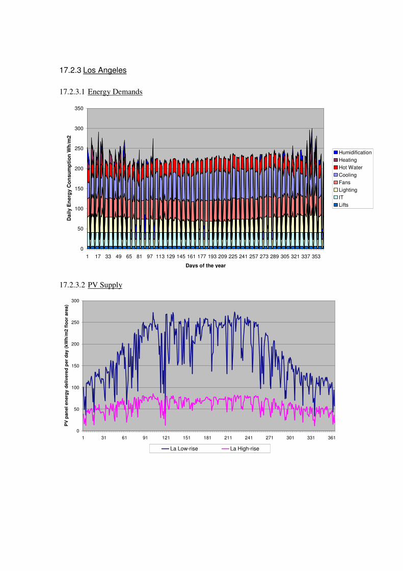
17.2.3 Los Angeles


0

50

100

150

200

250

300

350

1 17 33 49 65 81 97 113 129 145 161 177 193 209 225 241 257 273 289 305 321 337 353

Days of the year

Da

ily E

ne

rgy

Co

ns

um

pti

on

Wh

/m2

Humidification

Heating

Hot Water

Cooling

Fans

Lighting

IT

Lifts

17.2.3.2 PV Supply

0

50

100

150

200

250

300

1 31 61 91 121 151 181 211 241 271 301 331 361

PV

pa

ne

l e

ne

rgy

de

liv

ere

d p

er

da

y (

kW

h/m

2 f

loo

r a

rea

)

La Low-rise La High-rise

17.2.4 Dubai


0

50

100

150

200

250

300

350

1 17 33 49 65 81 97 113 129 145 161 177 193 209 225 241 257 273 289 305 321 337 353

Days of the year

Da

ily

En

erg

y C

on

su

mp

tio

n W

h/m

2

Humidification

Heating

Hot Water

Cooling

Fans

Lighting

IT

Lifts

17.2.4.2 PV Supply

0

50

100

150

200

250

300

350

1 31 61 91 121 151 181 211 241 271 301 331 361

PV

pa

ne

l e

ne

rgy

de

liv

ere

d p

er

da

y (

kW

h/m

2 f

loo

r a

rea

)

Dubai Low-rise Dubai High-rise

17.2.4.3 Hong Kong


0

50

100

150

200

250

300

350

1 17 33 49 65 81 97 113 129 145 161 177 193 209 225 241 257 273 289 305 321 337 353

Days of the year

Daily

En

erg

y C

on

su

mp

tio

n W

h/m

2

Humidification

Heating

Hot Water

Cooling

Fans

Lighting

IT

Lifts

17.2.4.5 PV Supply

0

50

100

150

200

250

300

1 31 61 91 121 151 181 211 241 271 301 331 361

PV

pa

ne

l e

ne

rgy

de

liv

ere

d p

er

da

y (

kW

h/m

2 f

loo

r a

rea

)

Hong Kong Low-rise Hong Kong High-rise

17.2.5 Singapore


0

50

100

150

200

250

300

350

1 17 33 49 65 81 97 113 129 145 161 177 193 209 225 241 257 273 289 305 321 337 353

Days of the year

Dail

y E

ne

rgy

Co

ns

um

pti

on

Wh

/m2

Humidification

Heating

Hot Water

Cooling

Fans

Lighting

IT

Lifts

17.2.5.2 PV Supply

0

50

100

150

200

250

300

1 31 61 91 121 151 181 211 241 271 301 331 361

PV

pan

el

en

erg

y d

eliv

ere

d p

er

day

(kW

h/m

2 f

loo

r are

a)

Singapore Low-rise Singapore High-rise

an investigation into the energy consumption of future

Documents