An Introduction to the Uniform Design for Industrial Experiments with Model Unknown

Kai-Tai Fang, Chair Prof.

Hong Kong Baptist University

Email:ktfang@hkbu.edu.hk

Hong Kong Society for QualityAugust 29, 2003

Ford Motor CompanyDear Prof. Fang,

I would like to invite you to visit Ford Motor Company form July 30 – August 1, 2002 to provide a seminar on “Uniform Design for Computer Experiments And Industrial Experiments”.

Ford Motor CompanyIn the past few years, we have tremendous in

using Uniform Design for computer experiments. The technique has become a critical enabler for us to execute “Design for Six Sigma” to support new product development, in particular, automotive engine design. Today, computer experiments using uniform design have become standard practices at Ford Motor Company to support early stage of product design before hardware is available.

Ford Motor CompanyWe would like to share with you our successful

real world industrial experiences in applying the methodology that you developed. Additionally, your visit will be very valuable for us to gain more insight about the methodology as well as to learn the latest development in the area.

Agus Sudjianto, Engineering Manager

Kai-Tai Fang at Ford Motor Company

Introduction

Statistical Experimental Designs

Design of experiment is a branch of statistics and has been playing an important role in development of sciences and new techniques, especially, in development of high-tech.

Experiments are performed almost everywhere nowadays, usually for the purpose of discovering something about a particular process or system.

Experimental design

A good experimental design should minimize the number of experiments to acquire as much information as possible.Knowledge discovery

Experiments, especially in high-tech experiments, have the following characteristics:

• Multi-factors

• Experimental domain is large

• Underlying model is unknown

Complexities

• Nonlinearity

• No analytic formula of the response surface

Experiments-- Underlying model is unknown

Example 1.In a biological experiment we wish to

explore the relationship between the growth time and the response . Assume the underlying model

is unknown. There are many ways to design this experiment based on different statistical models.

( )x ( )y

[ ] )1.2( , 20,x ,e-1y(x)y2-2x ∈==

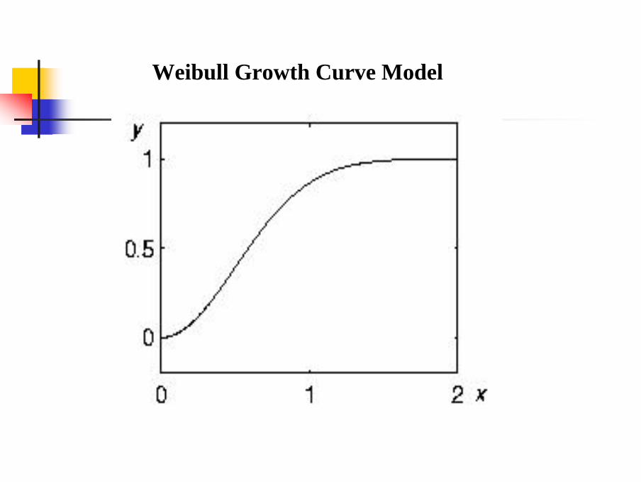
Weibull Growth Curve Model

The experimenter observes the response at several growth times, that are called levels. For each we repeat experiment times and related responses are A statistical model is

1. ANOVA Models

,x,,x q1 Ljx

jn.y,,y

jn1j jL

,n , 1,=i q, , 1,=j ,ε+µ=y jijjij LL

where is the true value and are random errors that are independently identically distributed according to

jµ ( )jxy ijε

).σ N(0, 2

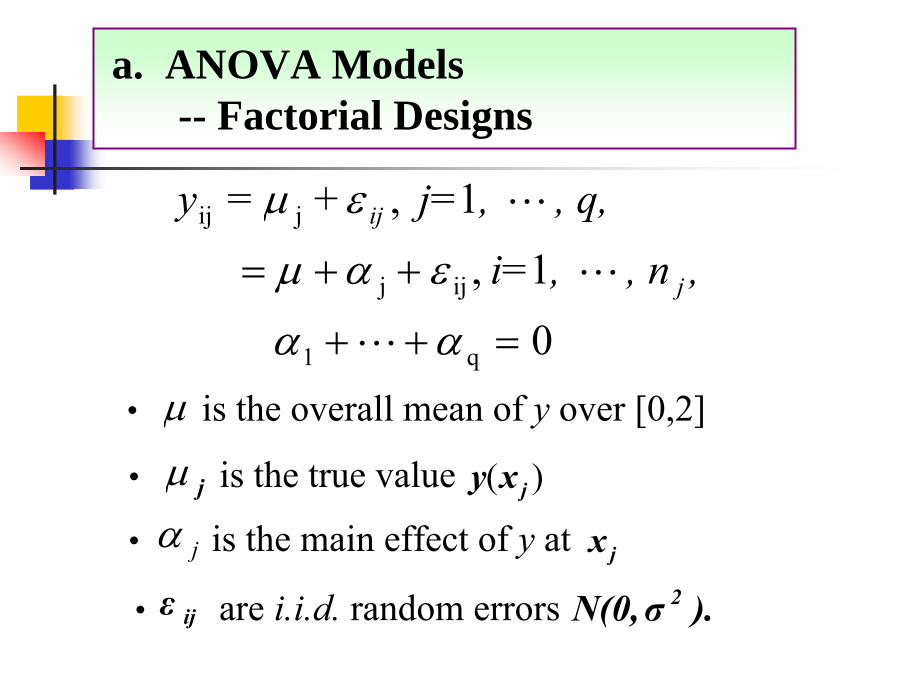
a. ANOVA Models-- Factorial Designs

0

1 ,

1 ,+ =

q1

ijj

jij

,, n, i=

, q, , j=y

j

ij

=++

++=

αα

εαµ

εµ

L

L

L

• is the true valuejµ )( jxy

• are i.i.d. random errorsijε ).σ N(0, 2

• is the overall mean of y over [0,2]µ

• is the main effect of y at jxjα

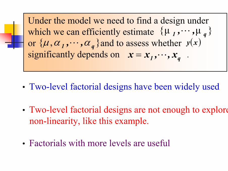
• Two-level factorial designs are not enough to explore non-linearity, like this example.

• Factorials with more levels are useful

Under the model we need to find a design under which we can efficiently estimate or and to assess whether significantly depends on .

}µ{µ q1 ,,L( )xy

q1 x ,,xx L=} ,{ q1 ,, ααµ L

• Two-level factorial designs have been widely used

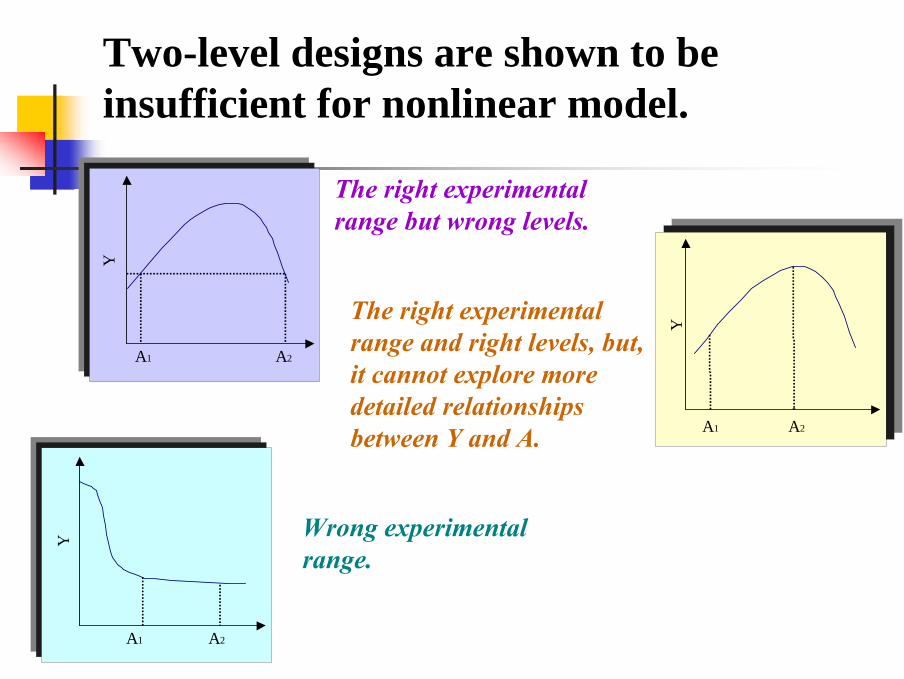
Two-level designs are shown to be insufficient for nonlinear model.

Y

A1 A2

Y

A1 A2

Y

A1 A2

Y

A2A1

Y

A2A1

Y

A2A1

The right experimental range but wrong levels.

The right experimental range and right levels, but, it cannot explore more detailed relationships between Y and A.

Wrong experimental range.

Y

A2A1

Y

A2A1

Y

A2A1

Factorial design with 4 levels

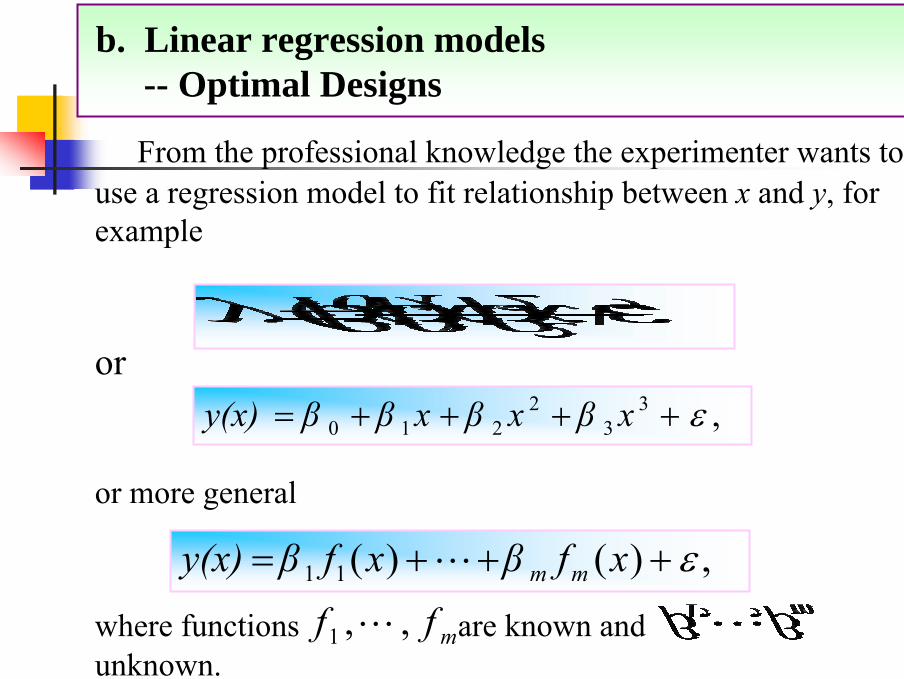
b. Linear regression models-- Optimal Designs

From the professional knowledge the experimenter wants to use a regression model to fit relationship between x and y, for example

or

or more general

where functions are known and unknown.

xβxβxββy(x) ,33

2210 ε++++=

,)()(11 ε+++= xfβxfβy(x) mmL

mff ,,1 L

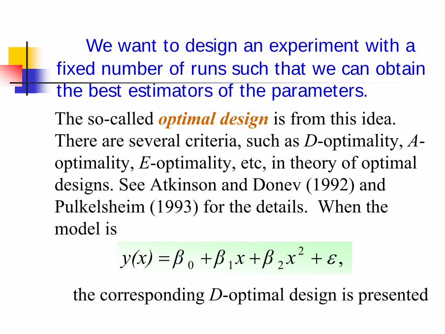
We want to design an experiment with a fixed number of runs such that we can obtain the best estimators of the parameters.The so-called optimal design is from this idea. There are several criteria, such as D-optimality, A-optimality, E-optimality, etc, in theory of optimal designs. See Atkinson and Donev (1992) and Pulkelsheim (1993) for the details. When the model is

the corresponding D-optimal design is presented

,2210 ε+++= xβxββy(x)

D-optimal design for second-order polynomial model

c. Nonparametric regression models-- Uniform Designs

g(x)y ,ε+=

where function g is unknown, can be employed.

When the experimenter do not have any prior knowledge about the underlying model, a nonparametric regression model

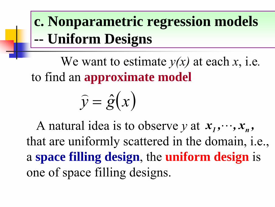
We want to estimate y(x) at each x, i.e. to find an approximate model

A natural idea is to observe y at that are uniformly scattered in the domain, i.e., a space filling design, the uniform design is one of space filling designs.

,x ,,x n1 L

( )xgy ˆ=)

c. Nonparametric regression models-- Uniform Designs

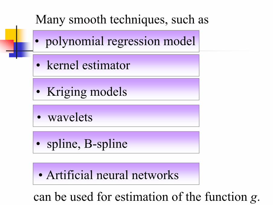
Many smooth techniques, such as

• polynomial regression model

• kernel estimator

• wavelets

• spline, B-spline

can be used for estimation of the function g.

• Artificial neural networks

• Kriging models

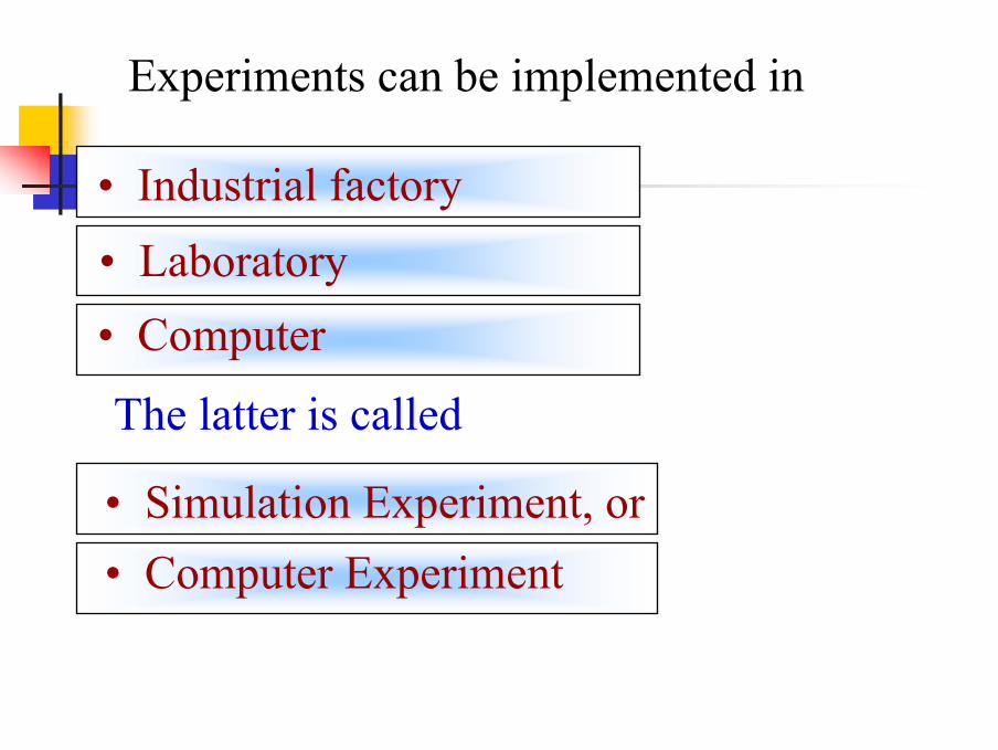
Experiments can be implemented in

• Industrial factory

• Computer• Laboratory

The latter is called

• Simulation Experiment, or• Computer Experiment

Uniform Design

Uniform designs

A demostrationexample

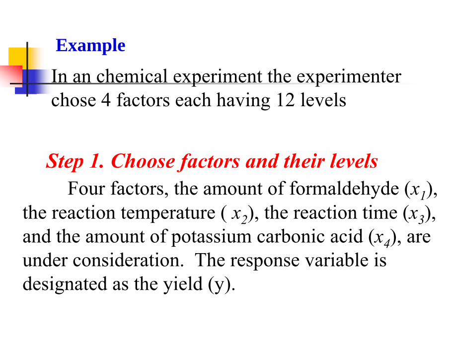
Four factors, the amount of formaldehyde (x1), the reaction temperature ( x2), the reaction time (x3), and the amount of potassium carbonic acid (x4), are under consideration. The response variable is designated as the yield (y).

Step 1. Choose factors and their levels

Example

In an chemical experiment the experimenter chose 4 factors each having 12 levels

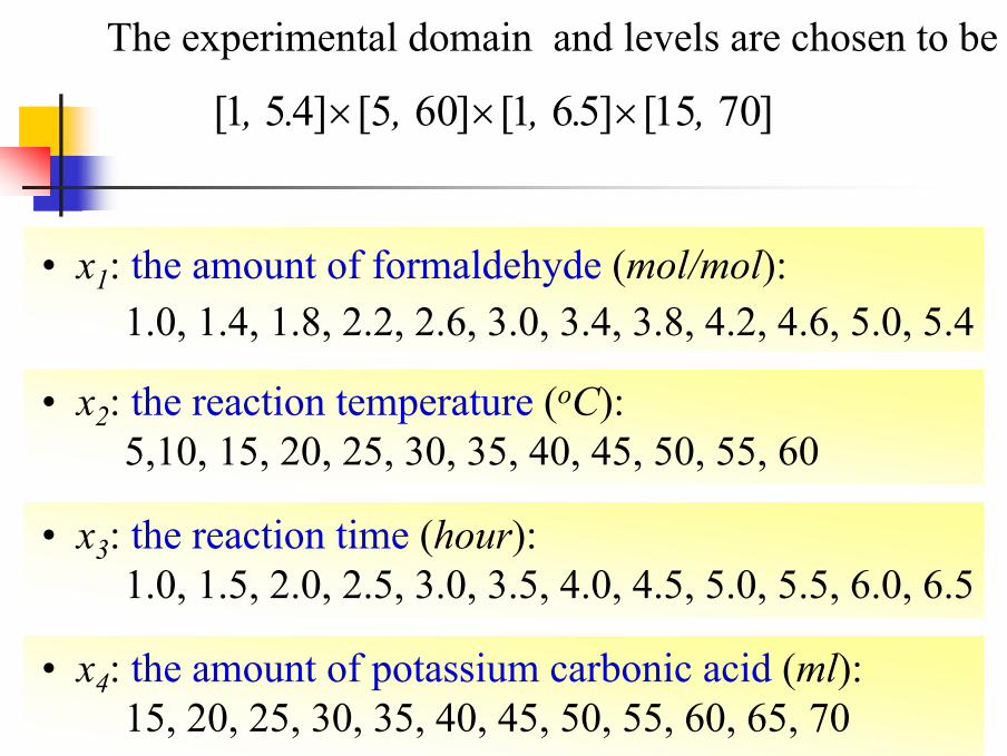
• x1: the amount of formaldehyde (mol/mol):1.0, 1.4, 1.8, 2.2, 2.6, 3.0, 3.4, 3.8, 4.2, 4.6, 5.0, 5.4

• x2: the reaction temperature (oC): 5,10, 15, 20, 25, 30, 35, 40, 45, 50, 55, 60

• x3: the reaction time (hour): 1.0, 1.5, 2.0, 2.5, 3.0, 3.5, 4.0, 4.5, 5.0, 5.5, 6.0, 6.5

• x4: the amount of potassium carbonic acid (ml): 15, 20, 25, 30, 35, 40, 45, 50, 55, 60, 65, 70

The experimental domain and levels are chosen to be

]7015[]561[]605[]451[ , ., , ., ×××

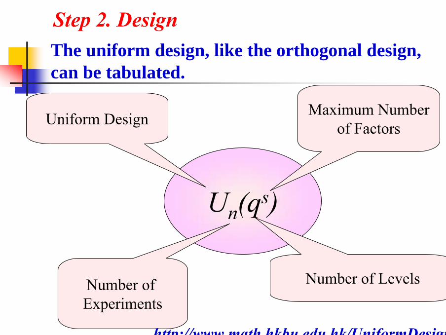
Un(qs)

Maximum Numberof Factors

Number of LevelsNumber of Experiments

Uniform Design

The uniform design, like the orthogonal design, can be tabulated.

http://www.math.hkbu.edu.hk/UniformDesign

Step 2. Design

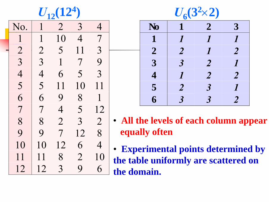
No 1 2 31 1 1 12 2 1 23 3 2 14 1 2 25 2 3 16 3 3 2

U6(32×2) No. 1 2 3 41 1 10 4 72 2 5 11 33 3 1 7 94 4 6 5 35 5 11 10 116 6 9 8 17 7 4 5 128 8 2 3 29 9 7 12 810 10 12 6 411 11 8 2 1012 12 3 9 6

U12(124)

• All the levels of each column appearequally often

• Experimental points determined by the table uniformly are scattered on the domain.

No. 1 2 3 41 11 8 2 102 9 7 12 83 8 2 3 24 10 12 6 45 1 10 4 76 2 5 11 37 4 6 1 58 7 4 3 129 6 9 8 110 3 1 7 911 5 11 10 1112 12 3 9 6

U12(124) Table

Step 2. Design

This experiment could be arranged with a UD table of the form U12(124), where nis a multiple of 7. It turns out that the experimenter chooses U12(124)design.

5.04.23.84.61.01.42.23.43.01.82.65.4

40351060502530204555515

1.56.52.03.52.56.01.03.04.54.05.55.0

605020304525357015556540

x1 x2 x3 x4No. 1 2 3 41 11 8 2 102 9 7 12 83 8 2 3 24 10 12 6 45 1 10 4 76 2 5 11 37 4 6 1 58 7 4 3 129 6 9 8 110 3 1 7 911 5 11 10 1112 12 3 9 6

No. 1 2 3 41 11 8 2 102 9 7 12 83 8 2 3 24 10 12 6 45 1 10 4 76 2 5 11 37 4 6 1 58 7 4 3 129 6 9 8 110 3 1 7 911 5 11 10 1112 12 3 9 6

No. 1 2 3 41 11 8 2 102 9 7 12 83 8 2 3 24 10 12 6 45 1 10 4 76 2 5 11 37 4 6 1 58 7 4 3 129 6 9 8 110 3 1 7 911 5 11 10 1112 12 3 9 6

5.04.23.84.61.01.42.23.43.01.82.65.4

40351060502530204555515

1.56.52.03.52.56.01.03.04.54.05.55.0

605020304525357015556540

x1 x2 x3 x4 y0.18360.17390.09000.11760.07950.01180.09910.13190.07170.01090.12660.1424

3. Run experiments

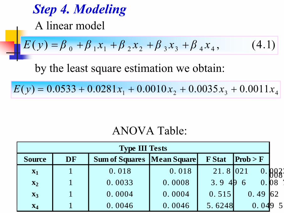
A linear model)1.4(,)( 443322110 xβxβxβxββyE ++++=

4321 0011.00035.00010.00281.00533.0)( xxxxyE ++++=

by the least square estimation we obtain:

Step 4. Modeling

Source DF Sum of Squares Mean Square F Stat Prob > FModel 4 0.0274 0.0069 8.2973 0.0086

Error 7 0.0058 0.0008

C Total 11 0.0332

Analysis of Variance

ANOVA Table:

Source DF Sum of Squares Mean Square F Stat Prob > Fx1 1 0.018 0.018 21.8021 0.0023

x2 1 0.0033 0.0008 3.9496 0.0872

x3 1 0.0004 0.0004 0.515 0.4962

x4 1 0.0046 0.0046 5.6248 0.0495

Type III Tests

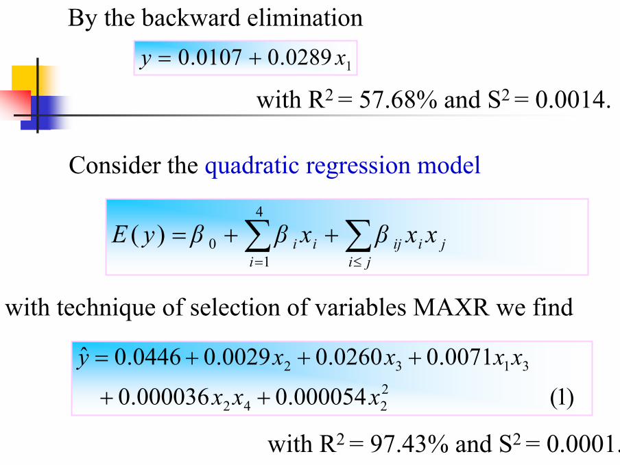
By the backward elimination

10289.00107.0 xy +=

with R2 = 57.68% and S2 = 0.0014.

Consider the quadratic regression model

xxβxββyEji

jiiji

ii )(4

10 ∑∑

≤=

++=

with technique of selection of variables MAXR we find

)1( 000054.0000036.0

0071.00260.00029.00446.0ˆ2242

3132

xxx

xxxxy

++

+++=

with R2 = 97.43% and S2 = 0.0001.

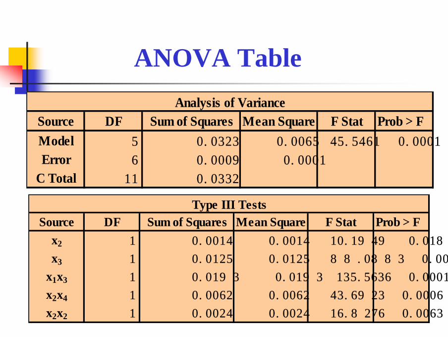
Source DF Sum of Squares Mean Square F Stat Prob > Fx2 1 0.0014 0.0014 10.1949 0.0188

x3 1 0.0125 0.0125 88.0883 0.0001

x1x3 1 0.0193 0.0193 135.5636 0.0001

x2x4 1 0.0062 0.0062 43.6923 0.0006

x2x2 1 0.0024 0.0024 16.8276 0.0063

Type III Tests

Source DF Sum of Squares Mean Square F Stat Prob > FModel 5 0.0323 0.0065 45.5461 0.0001

Error 6 0.0009 0.0001

C Total 11 0.0332

Analysis of Variance

ANOVA Table

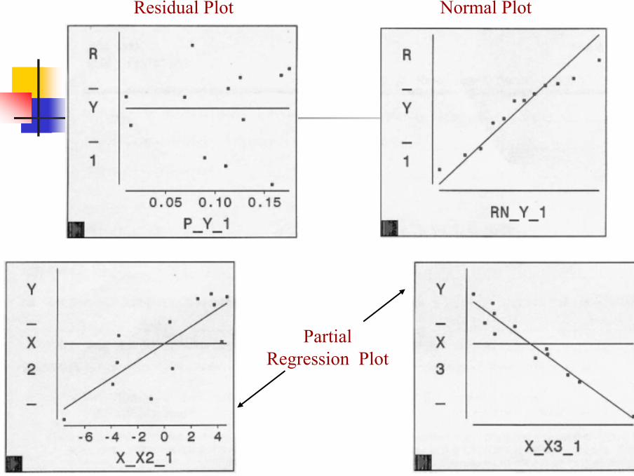
Residual Plot Normal Plot

Partial Regression Plot

Partial Regression Plot

}.7015,5.61},605,4.51:),,,{(

≤≤≤≤≤≤≤≤=

43

214321

x x x xxxxxD

that is to find such that

where is given by (1).

),,,( *4

*3

*2

*1 xxxx

),,,,(ˆmax),(ˆ 432141 xxxxy,xx,xxyD

** =*3

*2

),,,(ˆ 4321 xxxxy

Step 5. Prediction and optimization

By optimization algorithm, it is easily found that and the corresponding response

is the maximum70,1,2.50,4.5 ==== 4321 xxxx%.3.19ˆ =y

However, this is only a statistical prediction and further verification with confirmation experiments is needed.

Step 5. Prediction and optimization

Centered model

,)5.32(000082.0

)5.42)(75.3(00058.0 )5.42(00114.0 )5.32(000937.0)2.3(0281.01277.0ˆ

22

434

31

−+

−−+−+−+−+=

x

xxxxxy

with R2 = 97.05% and S2 = 0.0002.Normal Plot Residual Plot

(2)

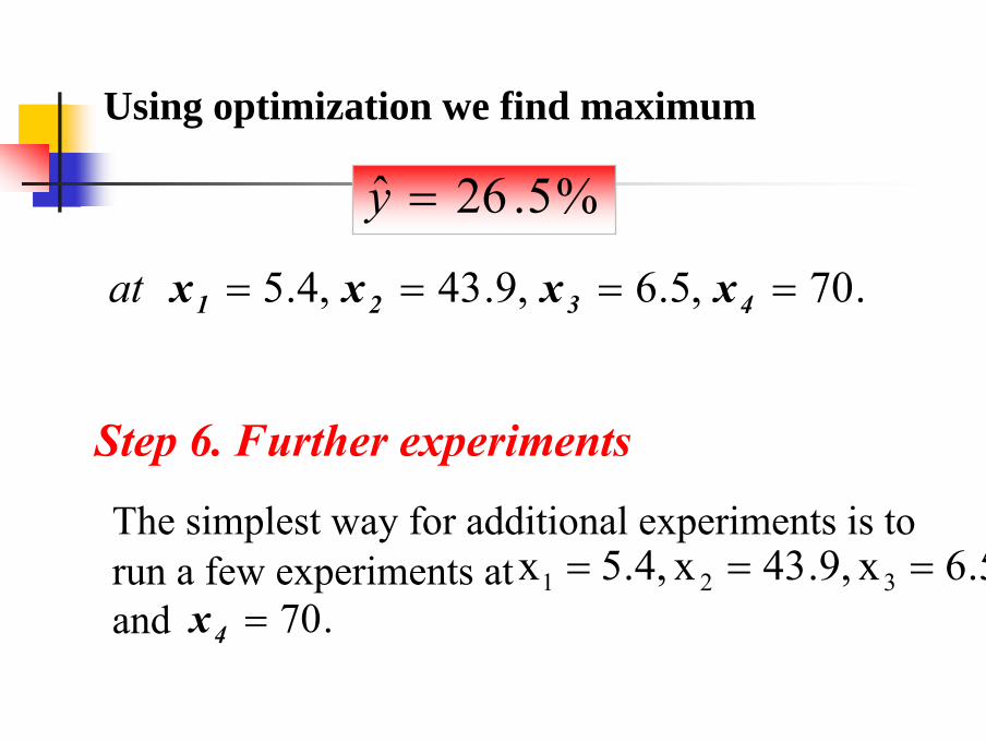
Using optimization we find maximum

%5.26ˆ =y

.70,5.6,9.43,4.5 ==== 4321 x x x x at

Step 6. Further experiments

The simplest way for additional experiments is to run a few experiments at and

,5.6x,9.43x,4.5x 321 ===.70=4x

Many smooth techniques, such as

• polynomial regression model

• kernel estimator

• Kriging models

• wavelets

• spline, B-spline

can be used for estimation of the function g.

• Artificial neural networks

Uniform designs

Historical review

In 1978 three big projects in system engineeringraised the same type of problems to me. It needs one day calculation in a computer to obtain the output y from the given input under the true model

Computer Experiments-- space filling design

xxgy s ).,,( 1 L=

where the function g has no analytic formula and y is the solution of a set of differential equations.

They wanted to choose a representative set of inputs, and related output

to find a good approximate model that is much simpler than the true one.

},{ n1 x ,,x L,n1 y ,,y L g

).,,(gy 1 sxx L=

approximate model

Computer Experiments

• Wang and Fang (1981) Chinese Sci. Bulletin

• Fang (1980)Acta Math. Appl. Sinica

The number of inputs of the interest in these three projects is at least 5 and the number of levels, q, of each input (factor), they expected, is at least 18. Since the experiment was expensive and the computational time is long, the number of runs, n, wished to be within 50. That is

,5≥s andq ,18≥ .50≤n

We ( Y. Wang and myself) proposed the uniform design.

Applications of approximation models

Visualizationestimationoptimizationothers

• Fang and Wang (1994) Number-Theoretic Methods in Statistics

• Fang and Hickernell (1995) Invited talk in the ISI 50th Session

• Fang, Lin, Winker and Zhang (2000) Technometrics

• Fang and Lin (2003) Handbook in Statistics: Statistics in

Industry

A comprehensive review can refer to

Uniform designs in computer experiments

Computer models are often used in science and engineering fields to describe complicated physical phenomena which are governed by a set of equation, including linear, nonlinear, ordinary, and partial differential equations. It may take a long time to find the output from the input under the true model

Uniform Design in Computer Experiments

).( 1 s, x, xg=y L

where the function g has no analytic formula.

A case study of computer experiments

In the study of the flow rate of water from an upper aquifer to a lower aquifer, the aquifers are separated by an impermeable rock layer but there is a borehole through that layer connecting them.

The model formulation is based on assumption of no groundwater gradient, steady-state flow from the upper aquifer into the borehole and from the borehole into the lower aquifer, and laminar, isothermal flow through the borehole.

The response variable y, the flow rate through the borehole in m3/yr, is determined by

where the 8 input variables are as follows:

.]1)[log(

][22)log(

2l

u

wwwrr

u

w TT

KrLT

rr

luu HHTy++

−=

π

length of borehole

radius of borehole:)(mrw

:)(mr:)/( 2 yrmTu

:)/( 2 yrmTl

:)(mH u

:)(mH l

:)/( yrmK w

:)(mL

radius of influence transmissivity of upper aquifer

transmissivity of lower aquifer

potentiometric head of upper aquifer

potentiometric head of lower aquifer

hydraulic conductivity of borehole

and the domain is given by

., K, L ,, H,, H

,,., T, T,, r,., .r

w

lu

lu

w

]120459855[],16801120[]820700[]1110990[

]116163[]11560063070[]50000100[]150050[

∈∈∈∈

∈∈∈∈

The input variables and the corresponding output are denoted by and y(x),respectively. This example has been studied by Worley (1987), An and Owen (2001) and Morris, Mitchell and Ylvisaker (1993).

),,( 81 xx L=x

A. Design of Experiment

From the inference of each variable to the output y, we sort 8 input variables into

and put them into three groups: and

The number of levels of each variable in these three groups is chosen as 16, 8, and 4, respectively.

rTTkHHL r ulwluw ≥≥≥≥≥≥≥

},,,{},{ wluw KLHHR }.,,{ rTT ul

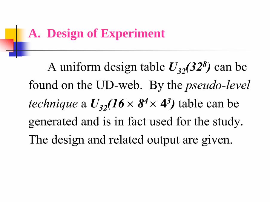
A uniform design table U32(328) can be found on the UD-web. By the pseudo-level technique a U32(16 × 84 × 43) table can be generated and is in fact used for the study. The design and related output are given.

A. Design of Experiment

Uniform Design and related output

The spatial modeling technique of kriging(Koehler and Owen (1996)) is based on a stationaryGaussian stochastic process and the Bayesian approach (Sacks, Welch, Mitchell and Wynn (1989) and Morris, Mitchell and Ylvisaker (1993)) uses the prior information.

B. Quadratic regression model

For the modeling, many authors proposed a number of methods. When the function g is a periodic, a Fourier regression model is recommended.

This model has an MSE=0.2578156.

)8914.8)(log(00087286.0)1050(0000068021.0

)760(0000071759.0)1400(70000002648.0

)760)(1050(000015325.0)10950(000090868.0

)1050(0035068.0)760(003554.0)1400(0007292.0

)3544.2)(log(9903.11560.4)log(

2

2

2

−−−−

−−

−+

−−+−+

−+−−−−

++=

rH

HL

HHK

HH

Lry

u

l

lu

w

u

l

w

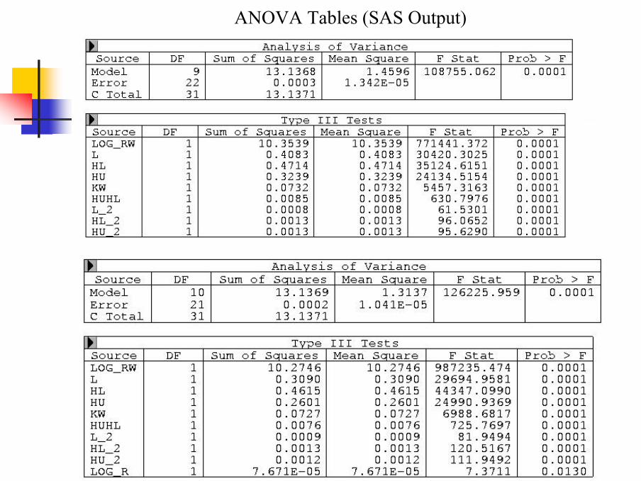
ANOVA Tables (SAS Output)

D. Comparisons among different designs and models

We compare the performances of different designs:

• Latin hypercube design• maximin design• maximin Latin hypercube design• modified maximin design

• uniform design

∑=

−=N

kkkN xyxyMSE

1

21 ,))(ˆ)((

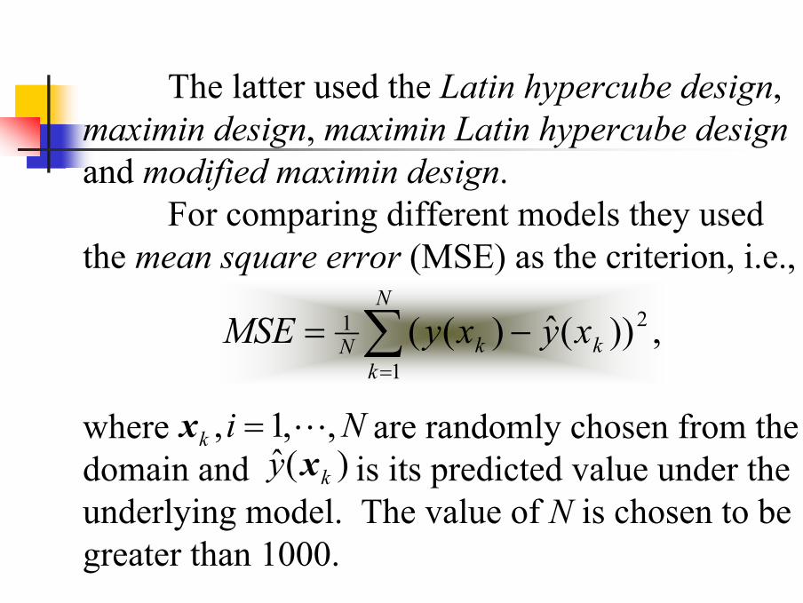
The latter used the Latin hypercube design, maximin design, maximin Latin hypercube designand modified maximin design.

For comparing different models they usedthe mean square error (MSE) as the criterion, i.e.,

where are randomly chosen from the domain and is its predicted value under the underlying model. The value of N is chosen to be greater than 1000.

Nik ,,1, L=x)(ˆ ky x

For comparing four different designs, Morris, Mitchell and Ylvisaker (1993) considered prediction errors at 400 random samples in the domain and at the 256 corner points of domain. They plot the prediction errors in two separated figures. Obviously, the B-spline model has large errors for the 256 corner points. This bias may be resulted from small number of levels for some input variables.

Ho and Xu (2000) employed the table U30(308) to design 30 level-combinations with the B-spline model mentioned above for modeling.

D. Comparisons among different designs and models

Prediction Errors at 400 Random Samples for Seven Design/Models

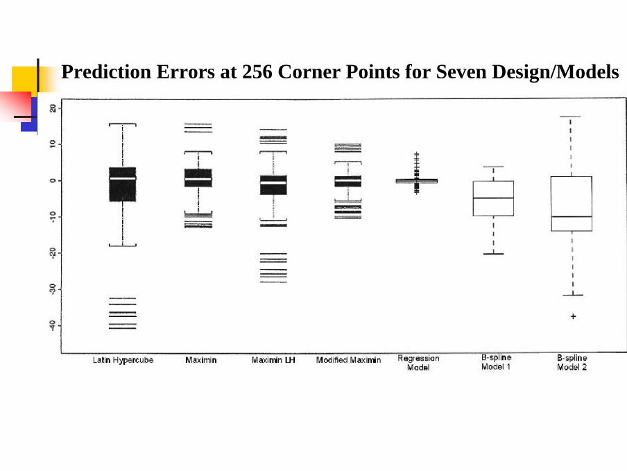
Prediction Errors at 256 Corner Points for Seven Design/Models

Uniform designs with mixtures

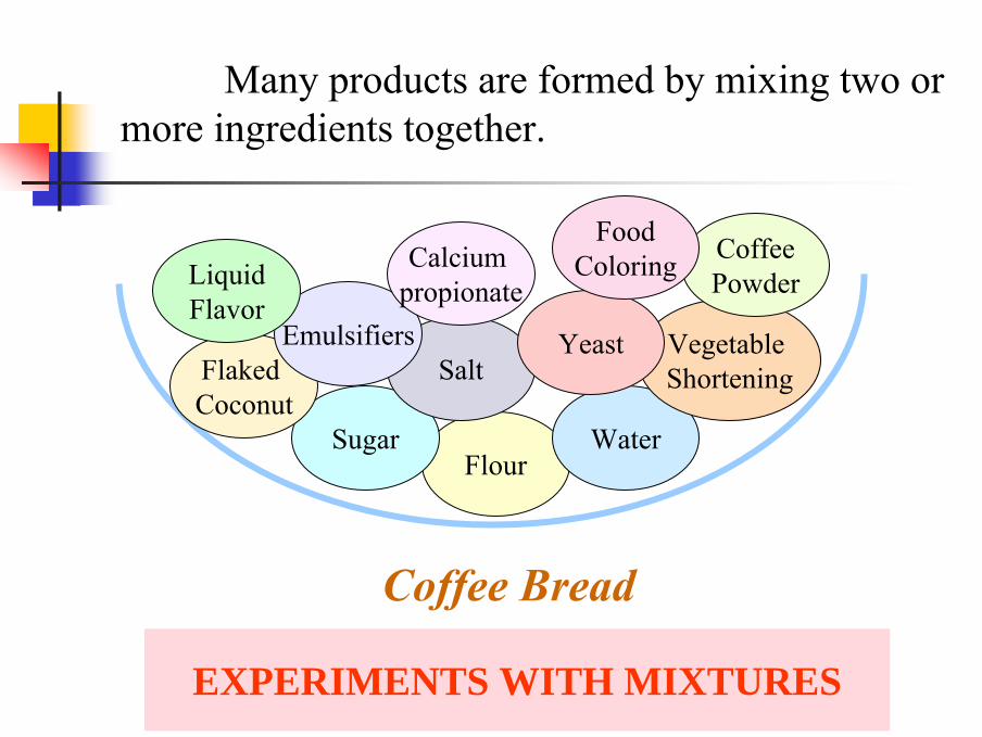
Many products are formed by mixing two or more ingredients together.

FlourWaterSugar

Vegetable ShorteningFlaked

CoconutSalt

YeastEmulsifiers

Calcium propionate

CoffeePowderLiquid

Flavor

FoodColoring

Coffee BreadHow to decide the proportions of the ingredients?

Experience ExperimentsEXPERIMENTS WITH MIXTURES

The UD can be utilized as

• a fractional factorial design

• a design of computer experiments

• a robust design

• a design with mixtures

UD SocietyThe UD has been used since 1980.

Several conference and workshops were held in the past yearsMore than 300 case studies of the use of UD during 1994 - 2000There is a nationwide society: Uniform Design Association of China since 1995

The First Conference, Beijing, 1995

Hong Kong Symposium, 1999

Hong Kong Symposium, 1999

Xian Conference, 2001

Comments on uniform design

Another approach to space-filling design using methods from number theory is briefly described in Exercise 7.7. This approach is reviewed by Fang, Wang and Bentler (1994) and its application in design of experiments discussed in Ch. 5 of Fang and Wang (1994). In the computer science literature the method is often called quasi-Monte Carlo sampling; see Neiderreiter (1992). --D.R. Cox and N. Reid (2000), The Thoery of the Design of Experiments.

Another type of space-filling design specifies points in the design space using methods from number theory. The resulting design is called a uniform, or uniformly scattered design. --D.R. Cox and N. Reid (2000), The Thoery of the

Design of Experiments.

Comments on uniform design

An important class of designs are so-called lattices. These have received considerable attention in number theory under ths heading of low discrepancy sequences. A principal text is Niederreiter (1992) and Fang and Wang (1994) (an their earlier work) make a considerable contribution in applications to statistics, including design. -- R.A. Bates, R.J. Buck, E. Riccomagno and H.P. Wynn (1996), JRSS-B, 58, 77-94 (with discussion).

Comments on uniform design

A case study by R.A. Bates, R.J. Buck, E. Riccomagno and H.P. Wynn (1996)

They considered a two-dimensional exercise for comparing Latin hypercube design, modified Latin hypercube design and lattice designs. They conclude:

Some conclusions are that the lattice designs do surprisingly well and a good integer lattice is robust against changes of criterion.

Comments on uniform design, by C.F.Jeff Wu and M. Hamada, p.445, “Experiments planing, analysis, and parameter design optimization.

If some of the noise factors have more than three levels, the run size of the orthogonal array for the noise factors may be too large. An alternative is to employ a smaller plan with uniformly spread point for the noise factors. These plans include Latin hypercube sampling (Koehler and Owen, 1996) and ``uniform’’ designs based on number-theoretic methods (Fang and Wang, 1994). Since the noise array is chosen to represent the noise variation, uniformity may be considered to be a more important required than orthogonality.

The UD entertains several advantages. It can explore relationships between the response and the factors with a reasonable number of runs and is shown to be robust to the underlying model specification.

Wiens D P, (1991) Stat. & Prob. Letters.Hickernell F J (1999) Stat. & Prob. Letters.Xie M Y and Fang K T, (2000) JSPI.

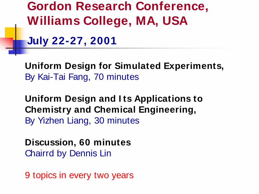
Uniform Design for Simulated Experiments,By Kai-Tai Fang, 70 minutes

Uniform Design and Its Applications to Chemistry and Chemical Engineering,By Yizhen Liang, 30 minutes

Discussion, 60 minutesChairrd by Dennis Lin

9 topics in every two years

Gordon Research Conference, Williams College, MA, USA

July 22-27, 2001

Uniform design

FlexibilityEasy to use

Easy to understand

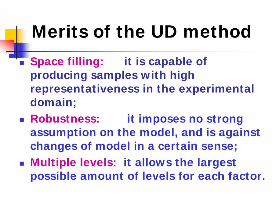
Merits of the UD methodSpace filling: it is capable of producing samples with high representativeness in the experimental domain;Robustness: it imposes no strong assumption on the model, and is against changes of model in a certain sense;Multiple levels: it allows the largest possible amount of levels for each factor.

Conclusion remarksThe UD can be utilized as

• a fractional factorial design

• a design of computer experiments

• a robust design

• a design with mixtures

.Thank you!

Contact information

Kai-Tai FangHong Kong Baptist University

Tel:3411-7025Fax:3411-5811

Email:ktfang@hkbu.edu.hkhttp://www.math.hkbu.edu.hk/UniformDesign

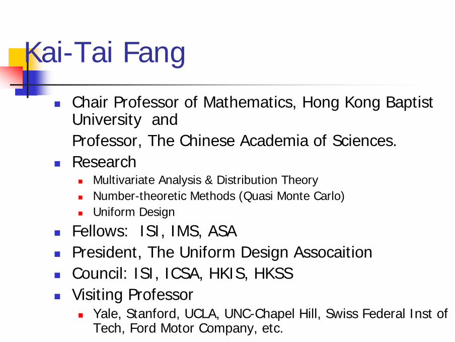
Kai-Tai FangChair Professor of Mathematics, Hong Kong Baptist University andProfessor, The Chinese Academia of Sciences. Research

Multivariate Analysis & Distribution TheoryNumber-theoretic Methods (Quasi Monte Carlo)Uniform Design

Fellows: ISI, IMS, ASAPresident, The Uniform Design AssocaitionCouncil: ISI, ICSA, HKIS, HKSSVisiting Professor

Yale, Stanford, UCLA, UNC-Chapel Hill, Swiss Federal Inst of Tech, Ford Motor Company, etc.