an introduction to the special issue on advances on
TRANSCRIPT
An Introduction to the Special Issue on Advances on Interactive Multimedia Systems
Z. Bojkovic 1, F. Neri 2
1 University of Belgrade, Belgrade, SERBIA, 2 Editor in Chief of WSEAS Transactions on Systems,
Department of Computer Science, University of Naples "Federico II", Naples, ITALY [email protected], [email protected]
This Special Issue intents to collect high-quality papers providing theoretical and/or practical matters dealing with advances on interactive multimedia systems (IMS). The perspective of today's information society calls for a multiplicity of devices including IP-enabled home appliances, personal computers, sensors, etc., all of which are globally connected. IMS have become important for information exchange and the core communication environment for business relations as well as for social interactions. Every day millions of people all over the world use interactive systems for a plethora of daily activities including searching, information access and exchange, multimedia communication enjoyment, buying and selling goods, keeping in touch with friends, etc. Current multimedia communication systems and architectural concepts must evolve to cope with complex connecting requirements. This is vital to the development of present day multimedia technologies as a natural step to all progression in general research about IMS. The fact that interactive multimedia is currently one of the fastest growing sectors in broadband networking, quality of service (QoS) standards and audio/video processing techniques must be taken into account. An IMS require real-time processing of data and media streams with the support of user interactions at any time. In this respect, the aim of the Special Issue is to highlight technological challenges in order to offer high-quality and low-delay multimedia services, together with designing a good user interface for smart interactive systems and the incorporation of automatic perception of human activities like presence, speech, interaction. The papers included have given a view point of advances on IMS by balancing the article selection between research and industrial community in order to include the high quality papers from both arenas. The contributions cover hot topics in the field and constitute one step among many others to recent progress in IMS. We start this Special Issue with the article entitled "Recognition of Assamese Spoken Words using a
Hybrid Neural Framework and Clustering Aided Apriori Knowledge". Artificial Neural Network based model is proposed for recognition of discrete Assamese speech, using a self Organizing Map-based phoneme count determination technique. It acts as a self sustaining, fully automated mechanism for spoken word recognition with 3, 4 and 15-phoneme variation. The second paper "Multimedia Signal Session in a Web Environment" includes the fields of health, IT, design, IMS and communications. The development provides new opportunities for interaction in telemedicine, particularly in the area of training and obtaining a surgical opinion in a Web environment. The presented system is technically feasible with high potential of medical staff training, which will result in a better patient care requiring surgery. The paper "New online RKPCA-RN Kernel method Applied to Tenessee Eastman Process" proposes a new method for online identification of a nonlinear system using a linear combination of Kernel functions applied to the used training set observations. Through several experiments the accuracy and good scaling properties of the proposed method have been demonstrated. The proposed method may be helpful in designing an adaptive control strategy of nonlinear systems. A unified approach in analysis of designs and reference software implementation of three generation for MPEG/ITU video coding standards is demonstrated in the paper "MPEG Video deployment in interactive multimedia systems: HEVC vs. AVC codec performance study". Bit reduction and coding gain based on peak-signal-to-noise ratio measure and complexity as well as encoding/decoding time of high efficient video coding (HEVC) vs. advance video coding (AVC) high profile (HP) are tested using the low-delay encoding constraints. Next, in the paper "Methods and Tools for Structural Information Visualization", it is emphasized that Higres, Visual Graph and ALVIS systems are aimed at supporting of structural information visualization on the base hierarchical
WSEAS TRANSACTIONS on SYSTEMS Z. Bojkovic, F. Neri
E-ISSN: 2224-2678 337 Issue 7, Volume 12, July 2013

graph modes. These systems are suited for visual processing and can be used in many areas where the visualization of structural information is needed. An algorithm framework for cross-layer QoS adaptation in multiservice heterogeneous environments is proposed based on Service-Oriented Architecture (SOA) principles in the paper "A Novel Algorithm for SOA-based Cross-Layer QoS Support in Multiservice Heterogeneous Environments". The proposed algorithm takes into account the diversity of user/application requirements networking technologies, terminal and provider capabilities. A proposal of framework for cross-layer QoS adaptation in order to support characteristics of various heterogeneous networking technologies, and to discover and select the proper network services that support QoS requirements for different applications, is presented, too. Finally, in the paper "Fuzzy Authentication Algorithm with Applications to Error Localization and Correction of Images", the proposed image
authentication methods have the ability to authenticate images even in the presence of small noise. They are in the position to localize errors as well as to correct them using the corresponding error correcting codes. Before we leave you to enjoy this Special Issue, we would like to thank all the authors, who invested a lot of work and effort providing their really valuable contributions as the results of their research work. These papers make a significant contribution to the problem of interactive multimedia systems. Of course, much work remains to achieve high quality technologies at low cost. Special thanks go to reviewers who dedicated their precious time in providing numerous comments and suggestions, criticism and constant and enthusiastic support. In closing, we hope that the contributions included should provide not only knowledge, but inspiration to researchers and developers of interactive multimedia systems.
WSEAS TRANSACTIONS on SYSTEMS Z. Bojkovic, F. Neri
E-ISSN: 2224-2678 338 Issue 7, Volume 12, July 2013

New online RKPCA-RN Kernel method Applied to Tennessee Eastman Process
NADIA SOUILEM, ILYES ELAISSI, OKBA TAOUALI & HASSANI MESSEOUAD
Unité de Recherche d’Automatique, Traitement de Signal et Image (ATSI), Ecole Nationale d’Ingénieur Monastir
Rue Ibn ELJazzar 5019 Monastir ; Tel : +(216) 73 500 511, Fax : + (216) 73 500 514, TUNISIA
[email protected]; [email protected]; [email protected]; [email protected]
Abstract: -This paper proposes a new method for online identification of a nonlinear system using RKHS models. The RKHS model is a linear combination of kernel functions applied to the used training set observations. For large datasets, this kernel based to severs computational problems and makes identification techniques unsuitable to the online case. For instance, in the KPCA scheme the Gram matrix order grows with the number of training observations and its eigen decomposition. The proposed method is based on Reduced Kernel Principal Component Analysis technique (RKPCA), to extract the principal component will be time consuming. Key-Words: - RKHS, RN, SLT, Kernel method, RKPCA, Online RKPCA-RN, Tennessee.
1 Introduction The last few years have registered the birth of a new modelling method of nonlinear systems using Reproducing Kernel Hilbert Space (RKHS) [1], [7], [15], [16], [17], [21], [22] called kernel methods. These methods have been applied to a large class of problems, such as face recognition [12], [24], time series prediction [4], identification of nonlinear system [11], [14], [23], …. The proposed method proceeds in two steps, first in an off line phase we select a set of kernels functions using the RKPCA technique, then in the online phase a RKHS model is constructed and successively updated. An eigen decomposition of Gram matrix can simply become too time-consuming to extract the principal components and therefore the system parameter identification becomes a tough task. To overcome this burden recently a theoretical foundation for online learning algorithm with kernel method in reproducing kernel Hilbert spaces was proposed [8], [10]. When the system to be identified is time varying, the online kernel algorithm is more useful, because these algorithms can automatically track changes of system
Behaviour with time-varying and time lagging characteristic. In this paper we propose a new method for online identification of a non linear system parameters modeled on Reproducing Kernel Hilbert Space (RKHS). This method uses the Reduced Kernel Principal Component Analysis (RKPCA) that selects the observations data to approach the Principal Components Analysis [11]. The selected observations are used to build an RKHS model with a reduced parameter number. The numbers of reduced observations are fixed and we actualise the parameters on minimizing a criterion. The proposed technique may be very helpful to design an adaptive control strategy of non linear systems. The paper is organized as follows. In section 2, we remind the Reproducing Kernel Hilbert Space (RKHS). In section 3, we remind the Reduced Kernel Principal Component Analysis RKPCA method. In section 4, we propose the new online RKPCA-RN method. The proposed algorithm has been tested to identify the nonlinear system and a Tennessee Eastman process.
WSEAS TRANSACTIONS on SYSTEMS Nadia Souilem, Ilyes Elaissi, Okba Taouali, Hassani Messeouad
E-ISSN: 2224-2678 339 Issue 7, Volume 12, July 2013

2 Reproducing Kernel Hilbert Space Let dX ⊂ ℝ an input space and ( )2 XL the Hilbert space of square integrable functions defined on X . Let 2:k X → ℝ be a continuous positive definite kernel. It is proved [18] that it exists a sequence of an orthonormal eigen functions ( )1 2, , ..., lψ ψ ψ in ( )2 XL and a sequence of corresponding real positive eigenvalues ( )1 2, , ..., lσ σ σ (where l can be infinite) so that:
( ) ( ) ( )1
, ; , l
j j jj
k x t x t x t Xσ ψ ψ=
= ∈∑ (1)
Let ( )2 XH L⊂ be a Hilbert space associated to the kernel k and defined by:
( )2
2
1 1
/ l l
ji i
i j j
wH f L X f w andϕ
σ= =
= ∈ = < + ∞
∑ ∑ (2)
Where i i iϕ σ ψ= 1, ...,i l= . The scalar product in the
space H is given by:
1 1 1
, , l l l
H i i j j H i ii j i
f g w z w zϕ ϕ= = =
< > = < > =∑ ∑ ∑ (3)
K is a Reproduisant Kernel for the space H if
* x X∀ ∈ , the function xk such as
:( ) ( , )
x
x
k X
t k t k x t
→=
ℝ
֏ (4)
is a function of the space H.
* x X∀ ∈ ; f H∀ ∈ , ( )x Hf k f x= (5)
H is a Reproducing Kernel Hilbert Space (RKHS) for the kernel k . The relation (5) describes the property of reproducibility of the function for the space H [1]. In other words the scalar product between each function
Hf ∈ and the function xk enables to determine ( )f x .
Let’s define the application Φ :
( )1
:( )
( )
l
l
X IR
x
x x
x
ϕ
ϕ
Φ →
Φ =
֏ ⋮ (6)
Where iϕ are given in (2). The kernel trick [1] is so that:
( )' ' ', ( ), ( ) ,k x x x x x x X= Φ Φ ∈ (7) Vapnik [18] proposes to adopt the (Structural Risk Minimisation: SRM)
( ) ( )( )1
21,
N
ii
i HD f V y f f
Nx λ
=
= +∑ (8)
Based on the representer theorem [19] the optimal function optf which minimizes ( )D f can be written as:
( ) ( )1
N
opt i ii
f x = a k x ,x=∑ (9)
Where , 1,...,ia i N= are the model parameters. 3 RKPCA method Let a nonlinear system with an input u∈ℝ and an output y∈ℝ from which we extract a set of observations { } 1, ..., N,i i iu y = . Let H an RKHS space with kernel k . To build the input vector
ix of the RKHS model we use the NARX (Nonlinear auto regressive with eXogeneous input) structure as:
{ }1,..., , ,..., ; ,u y
T
i i i m i i m u yx u u y y m m− − −= ∈ℕ (10)
The set of observations becomes { } 1, ...,,i i i ND x y ==
where 1u ym m
ix + +∈ℝ and iy ∈ℝ . and the RKHS model of this system based on (9) can be written as:
( )1
,N
j i i ji
y a k x x=
=∑ɶ (11)
WSEAS TRANSACTIONS on SYSTEMS Nadia Souilem, Ilyes Elaissi, Okba Taouali, Hassani Messeouad
E-ISSN: 2224-2678 340 Issue 7, Volume 12, July 2013

Let the application Φ :
( )
( )
( )
1
:
.
. .
l
l
X
x
x x
x
ϕ
ϕ
Φ →
Φ =
ℝ
֏ (12)
Where iϕ are given in (13). The Gram matrix K associated to the kernel k is an N - dimensional square matrix, so that:
( ), , for , 1, ..., i j i jk k x x i j N= = (13)
The kernel trick [1] is so that:
( ) ( ) ( )' ' ' , , , x x k x x x x X< Φ Φ > = ∈ (14)
We assume that the transformed data ( ){ } 1, ..., Nl
i ix
=Φ ∈ℝ
are centered [11]. The empirical covariance matrix of the transformed data is symmetrical and l - dimensional. It is written as following:
( ) ( )1
1 , M
T l li i
i
C x x CMφ φ
×
=
= Φ Φ ∈∑ ℝ (15)
Let 'l the number of the eigenvectors { } '1, ..., j j lV
=of the
Cφ matrix that corresponding to the non zeros positive eigenvalues { } '1, ..., j j l
λ=
. It is proved in [11]
that the number 'l is less or equal to N .
Due to the large size l of Cφ , the calculus of
{ }1, ..., j j l
V= '
can be difficult. The KPCA method shows
that these { }1, ..., j j l
V= '
are related to the eigenvectors
{ }1, ..., j j l
β= '
of the gram matrix K according to [11]:
( ) ',
1 , 1, ...,
N
j j i ii
V x j lβ=
= Φ =∑ (16)
Where ( ), 1, ... , Pj i jβ
= are the components of { }
1,...,j j lβ
= '
associated to their nonzero eigenvalues 1 ...l
µ µ> > '
The principle of the KPCA method consists in organizing the eigenvectors { }
1, ..., j j lβ
= ' in the
decreasing order of their corresponding eigenvalues { }
1, ..., j j lµ
= '. The principal components are the P first
vectors { }1, ..., Pj j
V=
associated to the highest
eigenvalues and are often sufficient to describe the structure of the data [11]. The number P satisfies the Inertia Percentage criterion IPC given by:
( )* arg 99P IPC= ≥ (17)
Where
1
1
*100
P
iiM
ii
IPCµ
µ
=
=
=∑
∑
(18)
The RKHS model provided by the KPCA method is [1].
( ),1 1
,P N
new q q i i newq i
y w k x xβ= =
=∑ ∑ɶ (19)
Since the principal components are a linear combination of the transformed input data ( ){ } 1, ...,i i N
x=
Φ
[12], the Reduced KPCA approaches each vector { }
1,...,j j PV
= by a transformed input data
( ) ( ){ } 1, ...,bj i i N
x x=
Φ ∈ Φ having a high projection value in
the direction of jV [5]. The projection of the ( )ixΦ on the jV called
( )i jxΦ ∈ɶ ℝ and can be written as:
( ) ( ), ; 1, ...,i j ijx V x j PΦ = Φ =ɶ (20)
According to (18) and (16), the relation (22) is written:
( ) ( ),1
, ; 1, ...,N
i j m m ijm
x k x x j Pβ=
Φ = =∑ɶ (21)
WSEAS TRANSACTIONS on SYSTEMS Nadia Souilem, Ilyes Elaissi, Okba Taouali, Hassani Messeouad
E-ISSN: 2224-2678 341 Issue 7, Volume 12, July 2013

To select the vectors ( ){ }bixΦ , we project all the
( ){ } 1, ...,i i Nx
=Φ vectors on each principal component
{ }1,...,j j P
V=
and we retained { } 1, ...,bj i i N
x x=
∈ that
satisfies
( ) ( )
( )
1, ...,
bj i jj i N
bj i j
x Max x
and
x ζ
=
≠
Φ = Φ Φ <
ɶ
(22)
Where ζ is a given threshold.
Once the { }1, ...,
bj j P
x=
corresponding to the P principal
component { } 1,...,j j PV
= are determined, we transform
the vector ( ) lxΦ ∈ℝ to the ( )ˆ PxΦ ∈ℝ vector that
belongs to the space generated by ( ){ }1,...,
bj
j Px
=Φ and
the proposed reduced model is:
( )1
ˆˆP
new j new jj
y a x=
= Φ∑ɶ (23)
Where :
( ) ( ) ( )ˆ , ; 1, ...,bnew j newj
x x x j PΦ = Φ Φ = (24)
And according to the kernel trick (7), the model (23) is:
( )1
ˆnew
P
j j newj
y a k x=
=∑ɶ (25)
Where:
( ) ( ), 1, ..., bj jk x k x x for j P= = (26)
The model (23) is less complicate than that provided by the KPCA. The identification problem can be formulated as a minimization of the regularized least square written as:
( ) ( )2
2
1 1
1ˆ ˆ ˆ2 2
N P
r i j j ii j
J a y a k x aρ
= =
= − +
∑ ∑ (27)
Where: ρ is a regularization parameter and
( )1ˆ ˆ ˆ, ... , T
Pa a a= is the parameter estimate vector The solution of the problem (27) is:
( ) 1*ˆ Pa F I Gρ −= + (28)
With :
( )
( )
( ) ( ) ( ) ( )
( ) ( ) ( ) ( )
11
1
1 1 11 1
11 1
and
N
i ii
P
N
b i ii
N N
i i i b ii i
P P
N N
b i i b i b ii i
k x y
G
k x y
k x k x k x k x
F
k x k x k x k x
=
=
= =×
= =
= ∈
= ∈
∑
∑
∑ ∑
∑ ∑
⋮ ℝ
⋯
⋮ ℝ
⋯
And P PPI ×∈ℝ is the P identity matrix
The RKPCA algorithm is summarised by the five following steps:
1. Determine the nonzero eigenvalues { }1,...,j j l
µ= '
and the eigenvectors { }1,...,j j l
β= '
of Gram
matrix K . 2. Order the { }
1,...,j j lβ
= ' on the decreasing way
with respect to the corresponding eigenvalues. 3. For the P retained principal components,
choose the ( ){ }1, ...,
bj
j Px
= that satisfy (22).
4. Solving (29) to determine *ˆ Pa ∈ℝ 5. The reduced RKHS model is given by (2)
WSEAS TRANSACTIONS on SYSTEMS Nadia Souilem, Ilyes Elaissi, Okba Taouali, Hassani Messeouad
E-ISSN: 2224-2678 342 Issue 7, Volume 12, July 2013

4 Online RKPCA-RN method
Prior to the online identification, we start with offline
identification on a set of observations { }1 1( , ), , ( , )n nD x y x y= … .
In this offline phase we apply the RKPCA technique
to reduce the number of the parameters of the RKHS
model. The model provided by the RKPCA is given
by:
( ) ( )1
,P
bj j
j
y x a k x x=
=∑ɶ (29)
The on line identification phase begins from the
instant 1n+ . At this instant a new couple of observations is available { }1 1,n nx y+ + .
From the equation (29), we calculate the output
RKHS model given by:
( )1 11
,P
bn j j n
j
y a k x x+ +=
=∑ɶ (30)
The error between the estimated output and the measured on actual one is:
( )1 1 1n n ne y y+ + += −ɶ (31)
If 1 1ne ε+ < (32)
where 1ε is a given threshold, we can say the model
approaches sufficiently the system behavior. If not, we update the parameters { }ja by minimizing the
criterion , 1r nJ +
( ) ( )
( )
2
, 1 11 1
22
1 11
1 ,2
1 ,2 2
P Pb b
r n n i j j ni j
Pb
n j j n nj
J A y a k x x
y a k x x Aρ
+ += =
+ +=
= − +
− +
∑ ∑
∑
(33)
Where
1
1P
n
P
a
A IR
a+
= ∈
⋮
We can write
( ) ( )2 2, 1 1 ( 1) 1 1 1
12r n n n P n n nJ A K A Y Aρ+ + + + + += − +
Where
( ) ( )
( ) ( )( ) ( )
1 1 1
( 1)( 1)
1
1 1 1
, . . . ,
. . . . .
. . . . .
, . . . ,
, . . . ,
b bP
P Pn P
b bP P P
b bn P n
k x x k x x
K IR
k x x k x x
k x x k x x
+ ×+
+ +
= ∈
and
1
11
1
b
Pn b
P
n
y
Y IRy
y
++
+
= ∈
⋮ (34)
The criterion (33) can be written as the following : ( )
( )( ) ( )
1
1
1
, 1 1
2 2( 1) 1 1 1
( 1) 1 1 ( 1) 1 1 1 1
min
1min2
1min2 2
Pn
Pn
Pn
r n nA IR
n P n n nA IR
T Tn P n n n P n n n n
A IR
J A
K A Y A
K A Y K A Y A A
ρ
ρ
+
+
+
+ +∈
+ + + +∈
+ + + + + + + +∈
=
− +
= − − +
(35) The minimum of , 1r nJ + is reached for :
, 1
1
0r n
n
J
A+
+
∂=
∂
( )( )
, 1
1
1 ( 1) 1 ( 1) 1 1 1 1
1 ( 1) ( 1) 1 1 ( 1) 11
1 ( 1) 1 1 1 1 1
1 .2 2
1 . . .2
. .
r n
n
T T T Tn n P n n P n n n n
T T T Tn n P n P n n n P n
n
T T Tn n P n n n n n
J
A
A K Y K A Y A AA
A K K A A K YA
Y K A Y Y A A
ρ
ρ
+
+
+ + + + + + + +
+ + + + + + ++
+ + + + + + +
∂=
∂
∂ − − + ∂
∂= −∂
− − +
(36)
As 1 ( 1) 1 1 ( 1) 1. et . .T Tn n P n n n P nA K Y Y K A+ + + + + + are scalar and
transposed, then
WSEAS TRANSACTIONS on SYSTEMS Nadia Souilem, Ilyes Elaissi, Okba Taouali, Hassani Messeouad
E-ISSN: 2224-2678 343 Issue 7, Volume 12, July 2013

, 1
1 ( 1) ( 1) 11 1
1 ( 1) 1 1 1 1 1
.
2. . .
r n T Tn n P n P n
n n
T T Tn n P n n n n n
JA K K A
A A
Y K A Y Y A Aρ
++ + + +
+ +
+ + + + + + +
∂ ∂= ∂ ∂
− − +
(37)
Therefore
( )
, 1( 1) ( 1) 1 ( 1) 1 1
1
( 1) ( 1) 1 ( 1) 1
r n T Tn P n P n n P n n
n
T Tn P n P P n n P n
JK K A K Y A
A
K K I A K Y
ρ
ρ
++ + + + + +
+
+ + + + +
∂= − +
∂
= + −
Then ( )-1
1 ( 1) ( 1) ( 1) 1 T Tn n P n P P n P nA K K I K Yρ+ + + + += + (38)
To every new observation, we apdate the parameters of the model (30) using the relation (38). Online RKPCA- NR algorithm Offline phase: According to (17) and (18) we determine the P retained principal components resulting from the processing of an N measurement set. 1- Then we determine the { }
1, ...,
bj j P
I x=
= set according
to (22), used during the online phase.
2- Write RKHS model obtained by RKPCA
( )1
,P
bn j j n
j
y a k x x=
=∑ɶ
Online phase:
For a new couple of observation { }1 1,n nx y+ +
1 - Calculate the output of the model RKHS
( )1 11
,P
bn j j n
j
y a k x x+ +=
=∑ɶ
2- Calculate the value of 1ne + . 3- If the condition (32) is satisfied⇒ we comes back to 1 for a new observation { }2 2,n nx y+ +
Otherwise: - Estimate the parameters { } 1, ...,ja j P= using
the relation (38).
5 Simulations The proposed method has been tested for modelling a nonlinear system and a Tennessee Eastman process.
5. 1 System nonlinear
We consider the nonlinear system
( )2( ) log ( 1) ( 2) 0.6 ( 2) 0.4 ( 1) 1 ( )y i u i u i y i y i e i= − − − + − + − + +
(39)
Where ( )e i is a gaussian noise. The input vector of RKHS model has the structure
[ ]( ) ( 1), ( 2), ( 1) Tx i u i u i y i= − − −
( )u i is the process input chosen as gaussian signal.
To build the RKHS model we use the ERBF Kernel (Exponential Radial Basis Function)
'
'
( , ) expx x
k x xµ
−
= −
(40)
With 5µ = and is the euclidean norm. The term
of regularisation 610 −λ = The chosen threshold is: 1 0.04ε = We performed the online identification using the online RKPCA-RN algorithm developed in section 4.
The number of observations in identification offline
phase is 150 and the number of principal component
analysis obtained by RKPCA method is equal to 5.
The number of observations in online identification
phase is 300.
The minimal normalized mean square error between
real output and estimated one (NMSE) is defined.
( )
( )
2
1
2
1
N
i ii
N
ii
y yNMSE
y
=
=
−=∑
∑
ɶ
(41)
Where iyɶ and iy design the model RKHS output
and the system output respectively.
WSEAS TRANSACTIONS on SYSTEMS Nadia Souilem, Ilyes Elaissi, Okba Taouali, Hassani Messeouad
E-ISSN: 2224-2678 344 Issue 7, Volume 12, July 2013

50 100 150 200 2502.2
2.4
2.6
2.8
3
3.2
3.4
3.6
3.8
sytem output
online RN-RKPCA
Figure 1: System and model outputs during the online
Identification In Figure 1, we represent the online RKPCA-RN output as well as the system output. We remark that the model output is in concordance with the system output, indeed the Normalized mean Square Error is equal to 0,002 . This shows the good performances of the proposed online identification method.
To evaluate the performance of the proposed method
we plot in Figure 2, the evolution of the NMSE.
50 100 150 200 250 300
1
1.5
2
2.5
3
3.5
4
4.5
x 10-3
iterations
NM
SE
Evolution of NMSE
Figure 2: Evolution of NMSE
5. 2 Tennessee Process To illustrate the efficiency of the proposed model we proceed to its validation on Tennessee Eastman process.
5. 2. 1 Process description
The Tennessee Eastman (TE) process [9] is a highly non linear, non-minimum phase, and open-loop unstable chemical process consisting of a reactor/separator/recycle arrangement. This process produces two products G and H from four reactants A, C, D and E. Also a byproduct F is present in the process. The simultaneous, irreversible and exothermic gas-liquid reactions are:
( ) ( ) ( ) ( )( ) ( ) ( ) ( )
( ) ( ) ( )( ) ( )
A g lig ,Product 1
A g lig ,Product 2
A g lig , byroduct
3 2 lig ,byroduct
C g D g G
C g E g G
E g F
D g F
+ + →
+ + →
+ →
→
The process has 12 valves available for manipulation and 41 measurements available for monitoring or control. The detailed description of these variables, process disturbances and base case operating conditions, is given in [3]. The process flowsheet is presented in Figure 3
Figure 3: Tennessee Process
WSEAS TRANSACTIONS on SYSTEMS Nadia Souilem, Ilyes Elaissi, Okba Taouali, Hassani Messeouad
E-ISSN: 2224-2678 345 Issue 7, Volume 12, July 2013

The modelling and the identification of the Tennessee Eastman process represent a challenge for the control community. It has been the subject of several studies [2] but most of them have tackled the process control without giving importance to modeling step. [13] have used input/ output process data to identify an autoregressive (AR) model parameters.
In our paper we intend to identify the parameters of the corresponding RKPCA- RN method of this process using the same technique of [20] for generating the data. 5. 2. 2 Data extraction The input/output data used to built the model were generated from the model of Tennessee implemented for the program Matlab © in the toolbox Simulink [9]. The process has 12 inputs and 41 outputs. According to the work of the process was divided into two fields. The first with a PID controller to maintain the process stability. The second field is devoted to the identification where only four inputs (reactor pressure, reactor level, D feed flow and E feed flow) are tuned and the others are maintained as suggested by mode 3 of Simulink model. Assuming the reactor outputs, we select the separator temperature product. 5. 2. 3 Knowledge model of Tennessee Process In this section, we consider for the knowledge model of the Tennessee process that suggested by [9] as shown by Figure 4.
Figure 4: Sheme input / output of Tennessee process * Output equations: The first output, separator temperature is given by:
( ), , , ,S CW S out CW S inT T T= − (42) Where:
, ,CW S outT Cooling water outlet temperature in the separator
, ,inCW ST Cooling water inlet temperature in the separator The temperature ST is linked to the energy
SQ removed for the separator by the differential equation:
( ).
, , , , , ,CW S p CW CW S out CW S inSQ m c T T= − (43)
Where:
,p CWC Specific heat capacity cooling water, kJ kg-1 K-1
,CW Sm Cooling water flow rate separator, kg h-1 For the second output, the reactor liquid level is given by:
,= ; , , , ,i rLr
i
NV i D E F G H
ρ=∑ (44)
Where: iρ Molar density of component i, mol m-3 ,
,i rN is the total molar holdup of the component i in the reactor.
5. 2. 4 Modelling in RKHS To generate the data from simulink, the simulation step size was 0.0005 s and the data were collected every 0.02 s. To build the RKHS model we use the Kernel RBF (Radial Basis Function)
'
'( , ) expx x
K x xµ
−= −
(45)
Where 120µ = , and is the euclidean norm. The
term of regularisation 610 −λ =
Reactor pression
E feed flow
Reactor level
Tennesse
Process
Separator temperature
Reactor liquid level
D feed flow
WSEAS TRANSACTIONS on SYSTEMS Nadia Souilem, Ilyes Elaissi, Okba Taouali, Hassani Messeouad
E-ISSN: 2224-2678 346 Issue 7, Volume 12, July 2013

The chosen threshold are: 1 0.01ε =
The number of observations in phase of identification
offline is 300 and the number of principal component
analysis obtained by RKPCA method is equal to 10.
The number of observations in online identification
phase is 5000.
In Figure 5, we represent the online RKPCA-RN output as well as the Tennessee Eastman output. We remark that the model output is in concordance with the system output, indeed the Normalized mean Square Error is equal to 65,6310− . This shows the good performances of the proposed online identification method.
500 1000 1500 2000 2500 3000 3500 4000 4500 500089
90
91
92
93
94
system output
online RN-RKPCA
Figure 5: Validation phase
To evaluate the performance of the proposed method
we plot in Figure 6, the evolution of the NMSE.
500 1000 1500 2000 2500 3000 3500 4000 4500 50000
1
2
3
4
5
6
7
8
x 10-6
iterations
NM
SE
Evolution of NMSE
Figure 6: Evolution of NMSE 6 Conclusion In this paper, we have proposed an online reduced kernel principal component analysis method for nonlinear system parameter identification. Through several experiments, we showed the accuracy and good scaling properties of the proposed method. This algorithm has been tested for identifying a nonlinear system and a Tennessee Eastman process and the results were satisfactying. The proposed technique may be very helpful to design an adaptive control strategy of non linear systems.
References:
[1] Aronszajn N. Theory of reproducing kernels. Transaction American Mathematical Society 68, 3,1950, pp. 337- 404,.
[2] Banerjee A and Arkun Y. Control configuration design applied to the Tennessee Eastman plant-wide control problem. Computers Chemical Engineering, 19, 1995, pp. 453-480.
[3] Downs, J.J and Vogel, E, A plant-wide industrial process control problem. Computers and Chemical Engineering, 17, 1993, pp245–255.
[4] Fernandez R. Predicting Time Series with a Local Support Vecto r Regression Machine. In ACAI conference, 1999.
WSEAS TRANSACTIONS on SYSTEMS Nadia Souilem, Ilyes Elaissi, Okba Taouali, Hassani Messeouad
E-ISSN: 2224-2678 347 Issue 7, Volume 12, July 2013

[5] Elaissi I, Modélisation, Identification et Commande Prédictive des systèmes non linéaires par utilisations des espaces RKHS, thèse de doctorat 2009, ENIT Tunisie.
[6] Elaissi I., Jaffel I., Taouali O. and Hassani M. Online prediction model based on the SVD–KPCA method. ISA Transactions, 2013.
[7] Fabien Lauer, Machines à Vecteurs de Support et Identification de Systèmes Hybrides, thèse de doctorat de l’Université Henri Poincaré – Nancy 1, octobre 2008, Nancy, France.
[8] Kuzmin D, Warmuth M.K, Online Kernel PCA with Entropic Matrix Updates, Proceedings of the 24 the International Conference on Machine Learning, 2007.
[9] Mauricio Sales Cruz, A.. Tennessee Eastman Plant –wide Industrial Process. Technical report, CAPEC, Technical University of Denmark,2004.
[10] Cedric Richard, Senior, José Carlos M. Bermudez, Paul Honeine, Online prediction of time series data with kernels, IEEE TRANSACTIONS ON SIGNAL PROCESSING, 57, 2009, pp1058-1067.
[11] Scholkopf B. and Smola A. et Muller K-R, Nonlinear Component analysis as Kernel eigenval problem, Neural computation. 10, 1998,pp 1299-1319.
[12] Scholkopf B. and Smola A., Learning with kernels. The MIT press, 2002. [13] Sriniwas R. and Arkun. Y. Control of the
Tennessee Eastman process using input–output models. Journal of Process Control, 7, 1997,pp. 387-400.
[14] Saidi N, Taouali O. and Messaoud H. Modelling of a SISO and MIMO nonlinear communicatio channe using two modelling techniques,WSEAS TANSACTION ON CIRCUITS AND SYSTEMS, Issue 6, Vol 8, 2009, pp 518-528.
[15] Taouali O. , Elaissi I. and Hassani M, Online identification of nonlinear system using reduced kernel principal component analysis. Neural Comput & Application, vol 21, 2012, pp161-169.
[16] Taouali O, Elaissi I., Garna T. and Messaoud H, A new approach for identification of MIMO nonlinear system with RKHS model WSEAS TRANSACTIONS on INFORMATION SCIENCE and APPLICATIONS, issue 7, Vol 7,2010.
[17]Taouali O,Saidi N.and Hassani M, Identification of Nonlinear MISO Process using RKHS and Volterra models, WSEAS TRANSACTIONS ON SYSTEMS, issue 6, Vol 8, 2009, pp 723-732.
[18] V.N. Vapnik, Statistical Learning Theory, Wiley New York., 1998.
[19] G. Wahba, An introduction to model building with Reproducing Kernel Hilbert Spaces. Technical report No 1020,Department of Statistics, University of Wisconsin-Madison, 2000.
[20] T. Ylöstalo and H. Hyötyniemi. Maps of Process Dynamics. Proceedings of EUROSIM'98 Simulation Congress, K. Juslin, Finland: Federation of European Simulation Societies, 2,1998, pp 225-229.
[21] Lingli Yu, Min Wu, Zixing Cai, Yu Cao. A particle filter and SVM integration framework for fault-proneness prediction in robot dead reckoning system. WSEAS TRANSACTIONS on SYSTEMS Vol. 10, No11, 2011, pp 363-375
[22] Neri F. Cooperative evolutive concept learning: an empirical study". WSEAS Transaction on Information Science and Applications, WSEAS Press (Wisconsin, USA),Vol. 2, issue 5, 2005,pp. 559-563.
[23] Zeghbib, A.; Palis, F.; Tesenov. G.; Shoylev, N.; Mladenov, V. Performance of surface EMG signals identification using intelligent computational methods. WSEAS transactions on systems, 2005,Vol. 4. Issue: 7, pp: 1118-1125.
[24] Sofianita binti Mutalib, marina binti yusoff, Shuzlina binti Abdul rahman, Baseline extraction algorithm for online signature recognition, WSEAS Transactions on Systems, 2009.
WSEAS TRANSACTIONS on SYSTEMS Nadia Souilem, Ilyes Elaissi, Okba Taouali, Hassani Messeouad
E-ISSN: 2224-2678 348 Issue 7, Volume 12, July 2013

Methods and Tools for Structural Information Visualization
V. N. KASYANOV
Laboratory for Program Construction and Optimization Institute of Informatics Systems
Lavrentiev pr. 6, Novosibirsk, 630090 RUSSIA
[email protected] http://pco.iis.nsk.su/~kvn Abstract: - In the paper, we consider a practical and general graph formalism called hierarchical graphs and graph models. It is suited for visual processing and can be used in many areas where the strong structuring of information is needed. We present also the Higres, Visual Graph and ALVIS systems that are aimed at supporting of structural information visualization on the base hierarchical graph modes. Key-Words: - Information visualization, Hierarchical graphs, Hierarchical graph models, Graph algorithm animation, Graph editor, Graph drawing, Graph visualization, Visualization system
1 Introduction Visualization is a process of transformation of large and complex abstract forms of information into visual form, strengthening user’s cognitive abilities and allowing them to take the most optimal decisions.
Graphs are the most common abstract structure encountered in computer science and are widely used for structural information representation [11, 21]. Many graph visualization systems, graph editors and libraries of graph algorithms have been developed in recent years. Examples of these tools include VCG [30], daVinci [7], Graphlet [13], GLT&GET [27], yEd [34] and aiSee [1].
In some application areas the organization of information is too complex to be modeled by a classical graph. To represent a hierarchical kind of diagramming objects, some more powerful graph formalisms have been introduced, e.g. higraphs [9] and compound digraphs [31]. The higraphs are an extension of hypergraphs and can represent complex relations, using multilevel "blobs" that can enclose or intersect each other. The compound digraphs are an extension of directed graphs and allow both inclusion relations and adjacency relations between vertices, but they are less general then the higraph formalism. One of the recent non-classical graph formalisms is the clustered graphs [6]. A clustered graph consists of an undirected graph and its recursive partitioning into subgraphs. It is a relatively general graph formalism that can handle many applications with hierarchical information, and is amenable to graph drawing.
Hence, there is a need for tools capable of visualization of such structures. Although some general-purpose graph visualization systems provide recursive folding of subgraphs, this feature is used only to hide a part of information and cannot help us to visualize hierarchically structural information. Another weak point is that usual graph editors do not have a support for attributed graphs. Though the GML file format, used by Graphlet, can store an arbitrary number of labels associated with graph elements, it is impossible to edit and visualize these labels in the Graphlet graph editor. The standard situation for graph editors is to have one text label for each vertex and, optionally, for each edge.
The size of the graph model to view is a key issue in graph visualization [11]. Large graphs pose several difficult problems. If the number of graph elements is large it can compromise performance or even reach the limits of the viewing platform. Even if it is possible to layout and display all the graph elements, the issue of viewability or usability arises, because it will become impossible to discern between nodes and edges of graph model. It is well known that comprehension and detailed analysis of data in graph structures is easiest when the size of the displayed graph is small. Since none of the static layouts can overcome the problems caused by large graphs, hierarchical presentation, interaction and navigation are essential complements in information visualization.
An algorithm animation visualizes the behavior of an algorithm by producing an abstraction of both the data and the operations of the algorithm [26]. Initially it maps the current state of the algorithm
WSEAS TRANSACTIONS on SYSTEMS V. N. Kasyanov
E-ISSN: 2224-2678 349 Issue 7, Volume 12, July 2013
into an image, which then is animated based on the operations between two succeeding states in the algorithm execution. Animating an algorithm allows for better understanding of the inner workings of the algorithm, furthermore it makes apparent its deficiencies and advantages thus allowing for further optimization.
Applications of graph algorithm visualization can be divided into two types according to the method they implement: interesting events and the data-driven method [4]. Methods of the first type are based on selection of events that occur during execution of an algorithm, for example, comparing the vertex attribute value or removing an edge. Methods of this type create some visual effects for each interesting event. Methods of the second type are based on data changing. During an operation, the memory status is changed, for example, the values of variables. Further these changes are visualized in some understandable way. In the simplest case such changes can be displayed in a form of a table of variable values. This approach is used in debuggers of integrated development environments.
The existing algorithm visualizers have several disadvantages. One of the major drawbacks is that if there is a need to build visualization of an algorithm arbitrarily close to the original algorithm, then it is necessary to build a new visualizer. As a rule, visualizers also do not show the correspondence between the algorithm instructions and the generated visual effects or do not allow reassignment of visual effects to the corresponding events.
In the paper, we consider a practical and general graph formalism called hierarchical graphs and graph models [14]. It is suited for visual processing and can be used in many areas where the strong structuring of information is needed [3, 15, 16, 17, 20, 21, 22, 23, 24, 25, 28, 29]. We present also the Higres, Visual Graph and ALVIS systems that are aimed at supporting of information visualization on the base hierarchical graph modes. The Higres system is a visualization tool and an editor for attributed hierarchical graphs and a platform for execution and animation of graph algorithms [12]. The Visual Graph system was developed to visualize and explore large hierarchical graphs that present the internal structured information typically found in compilers [32]. The ALVIS system was developed to build the algorithm visualization with the help of a flexible system of visual effects and using a visualized graph algorithm as an input parameter.
2 Hierarchical graphs and graph models 2.1 Hierarchical graphs Let G be a graph of some type, e.g. G can be an undirected graph, a digraph or a hypergraph. A graph C is called a fragment of G, denoted by C G, if C includes only elements (vertices and edges) of G. A set of fragments F is called a hierarchy of nested fragments of the graph G, if GF and C1C2, C2C1 or C1 C2= for any C1, C2 F.
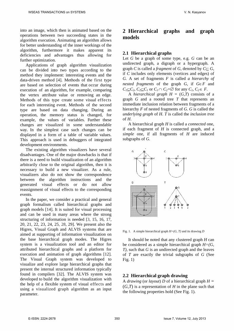
A hierarchical graph H = (G,T) consists of a graph G and a rooted tree T that represents an immediate inclusion relation between fragments of a hierarchy F of nested fragments of G. G is called the underlying graph of H. T is called the inclusion tree of H.
A hierarchical graph H is called a connected one, if each fragment of H is connected graph, and a simple one, if all fragments of H are induced subgraphs of G.
Fig. 1. A simple hierarchical graph H=(G, T) and its drawing D
It should be noted that any clustered graph H can be considered as a simple hierarchical graph H=(G, T), such that G is an undirected graph and the leaves of T are exactly the trivial subgraphs of G (See Fig. 1) 2.2 Hierarchical graph drawing A drawing (or layout) D of a hierarchical graph H = (G,T) is a representation of H in the plane such that the following properties hold (See Fig. 1).
WSEAS TRANSACTIONS on SYSTEMS V. N. Kasyanov
E-ISSN: 2224-2678 350 Issue 7, Volume 12, July 2013

Each vertex of G is represented either by a point or by a simple closed region. The region is defined by its boundary - a simple closed curve in the plane.
Each fragment of G is drawn as a simple closed region which include all vertices and subfragments of the fragment.
Each edge of G is represented by a simple curve between the drawings of its endpoints.
D is a structural drawing of H if all edges of any fragment of H are located inside the region of the fragment. A hierarchical graph is called a planar one if it has such a structural drawing that there are no crossing between distinct edges and the boundaries of distinct fragments. The following properties hold.
Theorem 1. There are nonplanar hierarchical graphs H=(G,T) with planar underlying graphs G.
Theorem 2. There are nonplanar hierarchical graphs H=(G,T) having nonstructural planar drawing.
Theorem 3. A simple connected hierarchical graph H=(G,T) is a planar graph if and only if there is such a planar drawing D of G that for any vertex p of T all vertices and edges of G-G(p) are in the outer face of the drawing of G(p). 2.3 Hierarchical graph models Let V be a set of objects called simple labels (e.g. V can include some numbers, strings, terms and graphs). Let W be a set of label types of graph elements and let a label set V(w)= V1 V2 … Vs, where s1 and for any i, 1 i s, Vi V, be associated with each w W.
A labelled hierarchical graph is a triple (H,M,L), where H is a hierarchical graph, M is a type function which assigns to each element (vertex, edge and fragment) h of H its type M(h) W, and L is a label function, which assigns to each element h of H its label L(h)V(M(h)).
The semantics of a hierarchical graph model is provided by an equivalence relation which can be specified in different ways, e.g. it can be defined via invariants (i.e. properties being inherent in equivalent labelled graphs) or by means of so-called equivalent transformations that preserve the invariants. 2.4 Hierarchical control flow graphs Many problems in program optimization have been solved by applying a technique called interval
analysis to the control flow graph of the program [10, 18]. A control flow graph which is susceptible to this type of analysis is called reducible.
Let F be a minimal set which includes G and is closed under the following property: if CF and p is such an entry vertix of C that subgraph {p} does not belong to F then F contains all maximum strongly connected subgraphs of graph which is obtained from C by removing of all edges which are ingoing in p. Let HF=(G,T) be such a simple hierarchical graph that T represents an immediate inclusion relation between fragments of the hierarchy F.
The following properties hold. Theorem 4. A control flow graph G is reducible
if and only if for the simple hierarchical graph HF=(G,T) the set of all fragments corresponding vertices pT is a hierarchy of nested single-entry strongly connected regions.
Theorem 5. A control flow graph G is reducible if and only if that for any pT of the simple hierarchical graph HF=(G,T) the fragment which is obtained from fragment corresponding to p by reducing all its inner fragments from F into their entry vertices is an interval.
3 The Higres system 3.1 Graph models in Higres A hierarchical graph supported by the Higres consists of vertices, fragments and edges which we call objects (See Fig. 2). Vertices and edges form an underlying graph. This graph can be directed or undirected. Multiple edges and loops are also allowed.
The semantics of a hierarchical graph is represented in Higres by means of object types and external modules (see below). Each object in the graph belongs to an object type with a defined set of labels. Each label has its data type, name and several other parameters. A set of values is associated with each object according to the set of labels defined for the object type to which this object belongs. These values, along with partitioning of objects to types, represent the semantics of the graph. New object types and labels can be created by the user. 3.2 Visualization In the Higres system each fragment is represented by a rectangle. All vertices of this fragment and all subfragments are located inside this rectangle.
WSEAS TRANSACTIONS on SYSTEMS V. N. Kasyanov
E-ISSN: 2224-2678 351 Issue 7, Volume 12, July 2013

Fragments, as well as vertices, never overlap each other. Each fragment can be closed or open (See Fig. 2). When a fragment is open, its content is visible; when it is closed, it is drawn as an empty rectangle with only label text inside it. A separate window can be opened to observe each fragment. Only content of this fragment is shown in this window, though it is possible to see this content inside windows of parent fragments if the fragment is open.
Most part of visual attributes of an object is defined by its type. This means that semantically relative objects have similar visual representation. The Higres system uses a flexible technique to visualize object labels. The user specifies a text template for each object type. This template is used to create the label text of objects of the given type by inserting labels' values of an object.
Fig. 2. The Higres system
Other visualization features include the
following: various shapes and styles for vertices; polyline and smooth curved edges; various styles for edge lines and arrows; the possibility to scale graph image to an
arbitrary size; edge text movable along the edge line;
colour selection for all graph components; external vertex text movable around the
vertex; font selection for labels text; two graphical output formats; a number of options to control the graph
visualization. Now Higres uses three graph drawing algorithms
for automatic graph allocation. The first one is a force method, which is very close to original
algorithm from [5]. The second one is our improvement of the first. The third one allocates rooted trees on layers. 3.3 The user interface The comfortable and intuitive user interface was one of our main objectives in developing Higres. The system's main window contains a toolbar that provides a quick access to frequently used menu commands and object type selection for creation of new objects. The status bar displays menu and toolbar hints and other useful information on current edit operation.
The system uses two basic modes: view and edit. In the view mode it is possible only to open/close fragments and fragment windows, but the scrolling operations are extended with mouse scrolling. In the edit mode the left mouse button is used to select objects and the right mouse button displays the popup menu, in which the user can choose the operation he/she wants to perform. It is also possible to create new objects by selecting commands in this menu. The left mouse button can be also used to move vertices, fragments, labels texts and edge bends, and resize vertices and fragments. All edit operations are gathered in a single edit mode. To our opinion, it is more useful approach (especially for inexperienced users) than division into several modes. However, for adherents of the last case we provide two additional modes. Their usage is optional but in some cases they may be useful: the "creation" mode for object creation and "labels" mode for labels editing.
Other interface features include the following: almost unlimited number of undo levels; optimized screen update; automatic
elimination of objects overlapping; automatic vertex size adjusting; grid with several parameters; a number of options that configure the user
interface; online help available for each menu, dialog
box and editor mode. 3.4 Algorithm animation To run an algorithm in the Higres system, the user should select an external module in the dialog box. The system starts this module and opens the process window that is used to control the algorithm execution. Higres provides the run-time animation of algorithms. It also caches samples for the repeated and backward animation. A set of
WSEAS TRANSACTIONS on SYSTEMS V. N. Kasyanov
E-ISSN: 2224-2678 352 Issue 7, Volume 12, July 2013

parameters is defined inside a module. These parameters can be changed by the user at any execution step. The module can ask user to input strings and numbers. It can also send any textual information to the protocol that is shown in the process window.
Fig. 3. Simulation of block-scheme representation of a program
A wide range of semantic and graph drawing algorithms can be implemented as external modules. As examples now we have modules that simulate finite automata, Petry nets and imperative program schemes (See Fig.3). The animation feature can be used for algorithm debugging, educational purposes and exploration of iteration processes such as force methods in graph drawing.
A special C++ API that can be used to create external modules is provided. This API includes functions for graph modification and functions that provide interaction with the Higres system. It is unnecessary for programmer, who uses this API, to know the details of the internal representation of graphs and system/module communication interface. Hence, the creation of new modules in the Higres system is a rather simple work.
4 The Visual Graph system 4.1 Visual Graph Visual Graph is a tool that automatically calculates a customizable multi-aspect layout of hierarchical graph models specified in GraphML (see below). This layout is then displayed, and can be interactively explored, extended and analyzed.
Visual Graph was developed to visualize and explore large graphs that present the internal structured information typically found in compilers.
Visual Graph reads a textual and human-readable GraphML-specification and visualizes the hierarchical graph models specified (See Fig. 4). Its design has been optimized to handle large graphs automatically generated by compilers and other applications.
Visual Graph provides tools for analyzing graph structures. Structural analysis means solving advanced questions that relate to a graph structure, for instance, determining a shortest path between two nodes.
Simple possibilities to extend the functionality of Visual Graph (for example, to add a new layout, search, analysis or navigating algorithm, a new tool for processing information associated with elements of graph models and so on) are provided. 4.2 GraphML GraphML (Graph Markup Language) [2] is a comprehensive and easy-to-use file format for graphs. It consists of a language core (known as the Structual Layer) to describe structural properties of one or more graphs and a flexible extension mechanism, e.g. to add application-specific data. Its main features include support of directed, undirected, mixed multigraphs, hypergraphs, hierarchical graphs, multiple graphs in a single file, application-specific data, and references to external data.
Two extensions, adding support of meta-information for light-weight parsers (Parse Extension) and typed attribute data (Attributes Extension) are currently part of the GraphML specification.
Unlike many other file formats for graphs, GraphML does not use a custom syntax. Instead, it is defined as an XML (Extensible Markup Language) sublanguage and hence ideally suited as an exchange format for all kinds of services generating or processing graphs 4.3 Reducing layout time Visual Graph was designed to explore large graphs that consist of many hundreds of thousands of elements. However, the layout of large graphs may require considerable time. Thus, there are two main ways to speed up the layout algorithm: multi-aspect layout of graph and control of layout algorithms.
The first way in visualizing a large graph is aimed at avoiding computing the layout of parts of the graph that are currently not of interest. Interactive exploring of graph is based on step by step construction of so-called multi-aspect layout of
WSEAS TRANSACTIONS on SYSTEMS V. N. Kasyanov
E-ISSN: 2224-2678 353 Issue 7, Volume 12, July 2013

graph being a set of drawings of some subgraphs of the graph. For presentation of multi-aspects layout a set of windows which includes a separate window for visualization of each considered subgraph is used. At each step of the construction a layout algorithm is applied to a subgraph being interested to user at this step. To indicate the interested subgraph the user can select its elements in the active window or in the navigator (see below). The user can also define some condition in the filter or in the search panel (see below). Then the condition will be used for searching of graph elements which will form the interested subgraph. The search can be performed both locally (in some part of graph, e.g. through a subgraph presented in the active window) or globally (around the entire graph). Multi-aspect drawing of graph models makes every visible part of the graph smaller, thus enabling the layout to be calculated faster and the quality of the layout to be improved.
Fig. 4. The Visual Graph system
In order to further reduce layout time, it is possible to control the layout algorithms, e.g. some layout phases can be omitted or the maximum number of iterations of some layout phases can be limited. However, this usually decreases the quality of the layout. The user can improve the layout by hand, e.g. by moving of nodes or changing of their sizes or forms. 4.4 Navigating through a graph Visual Graph offers several tools for navigating through a graph model: minimap, navigator, attribute panel, filter, search panel, notebook.
The minimap visualizes a working region of the graph model explored (See Fig. 4). It shows both the whole subgraph from the active windows and its visible part (i.e. such a subgraph part that is
allocated in the active window). It is possible to change both the visible part of the subgraph from the working region and scale of its drawing.
The navigator visualizes inclusion trees of hierarchical graph models as hierarchies of their vertices. It is possible to open in the active window any vertex of any group of vertices.
The attribute panel allows for elements of graph model in the working region choose attributes which should be visualized and ways of their visualization.
The filter is used for searching such elements of graph in the working region which satisfy given conditions (See Fig. 5).
The search panel is intended to search such elements of either whole graph model or its given part which satisfy given conditions.
The notebook can load files with additional information (e.g. with a source program being compiled) and associate it with graph elements.
5 The ALVIS system 5.1 Interactive visualization model
A new algorithm visualization model based on the dynamic approach and hierarchical graph models has been created. The main point of the suggested model is that the given algorithm is formulated in some programming language that allows us to use instructions operating with graphs and to execute the program derived from the text of the algorithm after a set of transformations. More details about the model can be found in [8]. The result of the program execution is information which is to be used in creation of the underlying algorithm visualization. An example of such instruction can be adding an edge or a change in the attributes of vertices. The following example shows the breadth-first search algorithm for any graph. In the given case, Get and Set instructions are used for reading and changing the graph element’s attribute values. These instructions have formats Get(Vertex, AttributeName) and Set(Vertex, AttributeName, A ttributeValue), respectively. To construct a visualization of the breadth-first search algorithm, the state attribute is appointed to each graph vertex. The value of the state attribute reflects whether the vertex was visited during graph traversal.
VertexQueue.Enqueue(Graph.Vertices[0]); while (VertexQueue.Count > 0)
WSEAS TRANSACTIONS on SYSTEMS V. N. Kasyanov
E-ISSN: 2224-2678 354 Issue 7, Volume 12, July 2013

{ Vertex v = VertexQueue.Dequeue(); Set(v, ”state”, ”visited”); foreach(Edge e in v.InEdges) { Vertex t =e.PortFrom.Owner; string c = Get(t, “state”); if(c != ”visited”) { Set(t, ”state”, ”visited”); VertexQueue.Enqueue(t); } } foreach(Edge e in v.OutEdges) { Vertex t = e.PortTo.Owner; string c = Get(t, “state”); if(c != ”visited”) { Set(t, ”state”, ”visited”); VertexQueue.Enqueue(t); } } } VertexQueue.Clear();
Fig. 5. The filter of the Visual Graph system
Each instruction of the algorithm generates one
or more images of the current state of the graph model. The graph model is an annotated hierarchical marked graph. It is useful to highlight the current executing instruction in each image because it allows a user to keep attention on valuable events at this moment. To solve the problem of highlighting the current executing instruction in the image, the following approach is used. Each text line of an algorithm can be
interpreted as a function. Also, each text line has a numeric index in all text lines. So that order value is added to arguments of the function corresponding to the text line. This additional parameter is the number of the current executing algorithm instruction. After this transformation, the text of the breadth- first search algorithm from the above example looks like this:
VertexQueue.Enqueue(Graph.Vertices[0]); while (WhileCondition(2, VertexQueue.Count > 0)) { Vertex v = VertexQueue.Dequeue(3); Set(4, v.ID, “state”, “visited”); foreach(Edge e in ForeachCollection(5, v.InEdges)) { Vertex t = e.PortFrom.Owner; string c = Get(7, t, ”state”); if(If Condition(8, c != ”visited”)) { Set(10, t, ”state”, ”visited”); VertexQueue.Enqueue(11, t); } } foreach(Edge e in ForeachCollection(13, v.OutEdges)) { Vertex t = e.PortTo.Owner; string c = Get(16, t, ”state”); if(If Condition(17, c != ”visited”)) {Set(19, t, ”state”, ”visited”); VertexQueue.Enqueue(20, t); } } } VertexQueue.Clear( ); The above example shows changes in the
attributes of the graph elements, too. This is a typical situation for algorithms implementing only traversal of a graph - a method when all graph vertices are visited one by one. For example, the Prüfer sequence of a given tree is generated by iteratively removing vertices from the tree until only two vertices remain. To perform this operation, the RemoveVertex( ) instruction should be used, which leads to generation of a visual effect of the corresponding vertex disappearing. Here is an example of the Prüfer encoding algorithm, how it can be formulated as a parameter of the graph algorithm visualization system:
WSEAS TRANSACTIONS on SYSTEMS V. N. Kasyanov
E-ISSN: 2224-2678 355 Issue 7, Volume 12, July 2013

int i = 0; List<Vertex> Leafs = new List<Vertex>( ); int n = Graph.Vertices.Count; while(i++ <= n-2) { Leafs.Clear(); foreach(Vertex v in Graph.Vertices) if(v.OutEdges.Count == 0) Leafs.Add(v); Vertex codeItem = Leafs[0].InEdges[0].PortFrom.Owner; Output.Add(codeItem);RemoveVertex(Leafs[0]); } Each algorithm instruction generates some
information during execution of the transformed text of the original algorithm. This information describes the number of the current instruction, the name of an attribute of a graph element, the previous value of the attribute, a new value of the attribute and the identifier of the graph element. This information allows us to get the full log of operations executed over graph elements. This operation log contains the detailed information on the state of the graph model during the algorithm running. Further the log of operations, the input graph and the original text of the algorithm can be used to generate the algorithm visualization. Each operation log entry corresponds to some graphical effect over visual representation of graph elements. The simplest example of the visual effect for the breadth-first search algorithm is to change the color of the graph vertex representation when a state attribute of the vertex has been changed and to change the color of the text of the corresponding instruction. 5.2 Algorithm visualization system The ALVIS system for graph algorithm visualization on the base of the described model has been constructed.
The system includes two main components: an algorithm execution module and a graph algorithm visualizer. It i s assumed that data are passed between these and other components of the system in a text form. It means that components of the system can be implemented on different platforms and with different tools.
The purpose of the algorithm execution module is to generate the execution log. The algorithm running is separated from its visualization. This allows us to perform the algorithm once and after that the operation log can be used to visualize and refine the visualization many times. This can be useful when computationally-intensive algorithms
are visualized. In such cases the second cycle of execution of the algorithm is complex.
To provide correct work of the algorithm execution module, it is necessary to meet a significant condition. Since any existing compiler or interpreter can be used to create this module, the algorithm must be formulated in the language supported by the selected compiler or interpreter. Actually this is not a restriction on the algorithm implementation language since many programming languages allow graph structures to be used in the program source code. So, the given algorithm text can be considered as a ready program source code. Also this allows us to transmit the input graph in this compiled program and to generate the log of operations.
Another significant restriction relates to the algorithmic complexity. In this approach, it is reasonable to visualize only efficient algorithms, because it will take much time to build the operation log of execution of an efficient algorithm. We can use a small input graph for this case. This assumption allows us to construct visualization for a reasonable time.
The algorithm execution module takes the given algorithm text in an appropriate programming language, executes it and returns the log of operations generated during the algorithm run on a particular graph. The log of executed operations contains information about all changed attributes of graph elements and about graph elements added or removed during the execution. Further this information is used to generate the algorithm visualization.
Another main component of the ALVIS system is the graph algorithm visualizer. At its input, this component receives the algorithm text, the input graph, the log of operations and additional graphical options. A log information item is added by special instructions created at the stage of preparation of the algorithm text. For example, these special instructions are the functions: Set( ), Get( ), IfCondition( ), WhileCondition( ) and ForeachCollection( ). Their first argument is the number of the corresponding text line. IfCondition( ) and WhileCondition( ) do not perform any changes in the graph model state but at least allow us to make a visual selection of the text line where it was inserted. ForeachCollection( ) is to be used to generate information which allows highlighting a set of vertices before they will be actually enumerated. To add these functions into appropriate places of the original algorithm, it is sufficient to use a contextual replacement. The purpose of the preparation stage is to eliminate the
WSEAS TRANSACTIONS on SYSTEMS V. N. Kasyanov
E-ISSN: 2224-2678 356 Issue 7, Volume 12, July 2013

need for declarative structures, which have no relation to the actual nature of the algorithm.
A log item may also contain information about the value of an attribute of a graph element. A graph element is a vertex, an edge or a port. If there is a vertex with its incident edge, then a port is a point where the edge enters the vertex. When rendering, it can be useful that the points are allocated for these additional objects. Ports simplify calculation of coordinates of graphical primitives which represent the edge elements. Strictly mathematically, it is possible to simulate a port with a labeled vertex. So the class of graphs with ports is isomorphic to the class of all graphs.
An attribute of a vertex, an edge or a port can have a string name and a string value. The log of operations stores the previous value of the attribute for a particular graph element. This information is also useful for building the visualization, since it is possible to make a smooth visual effect from a previous value of an attribute to its new value.
It is not obvious how to bind information from a log item to the visual effect. In this case, a user needs to interfere in order to set an explicit binding between the set of attributes in the text of the algorithm and the desired visual effects. For example, if the operation of a log item is about changing the coordinates of the graph element reflected with the use of the attribute “position”, then it is reasonable to bind the attribute with the visual effect, which leads to a shift of the graph element. Another user example is to bind all log items to the effect of a color mark of a current graph element under processing. It can be a current vertex visited in the algorithm of depth-first search or in any other graph traversal. In this aspect the suggested approach is close to the interesting events approach, where an algorithm instruction is an interesting event.
Fig. 6. Visualization of the depth-first search algorithm
Fig. 6 shows an example of visualization of the depth-first search algorithm on the graph, which is actually a binary tree. It is one of the screenshots taken during the process of visualization of the depth-first search algorithm. The left side of the figure displays the text of the algorithm formulated in terms of graph operations. The attribute of a graph vertex state indicates the fact that the vertex has already been visited during the process of the graph traversal. A line of the algorithm text has one of the following states: dark thin, light thin and thick. The first state means that the instruction has been executed at least once. The second state means that the current image and the last shown visual effect is the result of this instruction. The last state means that the instruction has not been executed yet. The right part of the figure displays the graph model, which is a hierarchical graph with attributes. Only if this attribute is set, the corresponding attribute will be created during visualization. In this example, the visited vertices get the state attribute that changes the color of a vertex. Also, this attribute’s value corresponds to the increase of line width showing the graph vertex circle. Vertices shown in a thin line have not been visited yet.
Displaying of additional data structures can also be used to improve understanding of visualization of a graph algorithm. For example, the depth-first search algorithm uses a stack and the breadth-first search algorithm visualization uses a queue. The content of a stack or a queue can be represented as a graph. Since the visualization system allows us to use the hierarchical graphs, a stack graph or a queue graph can be included into a graph model for a particular visualization. So the working graph model consists of a graph with two vertices. The first vertex contains a stack graph and the second contains an input graph. Such graph model can be visualized with the created module of the system of graph algorithm visualization. The queue or stack size is changed during execution of the given algorithm and the corresponding vertices are added or removed from the stack graph. Hierarchical graphs are helpful for this purpose. If there is no stack or queue, then a tree of fragments only consists of one fragment, the input graph. For a stack the graph model consists of three fragments: a root and two children. The first child is the input graph and the second is a graph representation of the stack. So, if the given algorithm uses an input graph and N additional structures, then the tree of fragments contains N+2 elements. It is a root element and its N+1 children,
WSEAS TRANSACTIONS on SYSTEMS V. N. Kasyanov
E-ISSN: 2224-2678 357 Issue 7, Volume 12, July 2013

one of which is the input graph and others are graph representations of additional data structures. 6 Conclusion In the paper, a practical and general graph formalism of hierarchical graphs and graph models was considered. It is suited for visual processing and can be used in many areas where the visualization of structural information is needed
The Higres system being a visualization tool and an editor for attributed hierarchical graphs and a platform for execution and animation of graph algorithms was presented. The Visual Graph system intended to visualize and explore large hierarchical graphs that present the internal structured information typically found in compilers was considered. The ALVIS system which builds the algorithm visualization with the help of a flexible system of visual effects and using a visualized graph algorithm as an input parameter was described.
The described methods and systems will be used in Web-Encyclopedia of Graph Algorithms (WEGA) [33] which is under development on the basis of our book [19] and is aimed to be not only a reference manual on graph algorithms but also an introduction to the graph theory and its applications to computer science.
In contrast to Donald Knuth who used the assembly language of the so-called MIX computer in his fundamental books “The art of computer programming”, we decided to use a high-level and language-independent representation of graph algorithms in our book and system. In our view, such an approach is preferential, as it allows us to describe algorithms in a form that admits direct analysis of their correctness and complexity, as well as a simple translation of algorithms to high-level programming languages without disturbance of their correctness and complexity. Besides, the described approach allows the readers to understand an algorithm at the informative level, to evaluate its applicability to a specific problem, and to make all its modifications needed for correct application of the algorithm.
We also believe that visualization could be very helpful for readers in understanding graph algorithms, and we plan to embed capabilities of interactive animation of graph algorithms which will be described into the WEGA system.
The author is thankful to all colleagues taking part in the projects described. The work was
partially supported by the Russian Foundation for Basic Research (grant N 12-07-0091). References: [1] aiSee http://www.absint.com/aisee/ [2] U. Brandes, M.S. Marshall, and S.C. North,
Graph data format workshop report, Lecture Notes in Computer Science, Vol. 1984, 2001, pp. 410–418.
[3] F. Colas, J.-Y. Dieulot, P-J. Barre, P. Borne, Dynamics modeling and causal ordering graph representation of a non minimum phase flexible arm fixed on a cart, WSEAS Transactions on Computers, Vol. 5, Issue 1, 2006, p 225-232.
[4] C. Demetrescu, I. Finocchi, J.T. Stasko, Specifying algorithm visualizations: interesting events or state mapping? Lecture Notes in Computer Science, Vol. 2269, 2002, pp.16–30.
[5] P. Eades, A heuristic for graph drawing, Congressus Numerantium, Vol. 42, 1984, pp. 149-160.
[6] Q.W. Feng, R.F. Cohen, P. Eades, Planarity for clustered graphs, Lecture Notes in Computer Science, Vol. 979, 1995, pp. 213-226.
[7] M. Fröhlich, M. Werner, Demonstration of the interactive graph visualization system daVinci, Lecture Notes in Computer Science, Vol. 959, 1995, pp. 266-269.
[8] D.S. Gordeev, Graph algorithm visualization: interpretation of algorithm as a program, Informatics in Research and Education, Novosibirsk, 2012, pp. 149-160. (In Russian).
[9] D. Harel, On visual formalism, Comm. ACM, Vol. 31, No. 5, 1988, pp. 514-530.
[10] M.S. Hecht, Flow Analysis of Computer Programs, New York, Elsevier, 1977.
[11] I. Herman, G. Melançon, M.S. Marshall, Graph visualization and navigation in information visualization: a survey, IEEE Transactions on Visualization and Computer Graphics, Vol. 6, 2000, pp. 24-43.
[12] Higres http://pco.iis.nsk.su/higres [13] M. Himsolt, The Graphlet system (system
demonstration), Lecture Notes in Computer Science, Vol. 1190, 1997, pp. 233-240.
[14] V.N. Kasyanov, Hierarchical graphs and graph models: problems of visual processing, Problems of Informatics Systems and Programming, Novosibirsk, 1999, pp. 7-32. (In Russian)
[15] V.N. Kasyanov, Support tools for graphs in computer science, Proc. of the 15th ACM SIGCSE Conference on Innovation and
WSEAS TRANSACTIONS on SYSTEMS V. N. Kasyanov
E-ISSN: 2224-2678 358 Issue 7, Volume 12, July 2013

Technology in Computer Science Education (ITiCSE 2010), ACM Press, 2010, p.315.
[16] V.N. Kasyanov, Information visualization on the base of hierarchical graph models, Advances in Applied Information Science. Proc. of AIC’12 and BEBI’12, WSEAS Press, 2012, pp. 115-120.
[17] V.N. Kasyanov, Hierarchical graph models and information visualization, Proceedings of the 2012 Third World Congress on Software Engineering (WCSE 2012), IEEE Computer Society, 2012, pp. 79-82.
[18] V.N. Kasyanov, V.A. Evstigneev, Graph Theory for Programmers. Algorithms for Processing Trees, Kluwer Academic Publ., 2000.
[19] V.N. Kasyanov, V.A. Evstigneev, Graphs in Programming: Processing, Visualization and Application, St. Petersburg, BHV-Petersburg, 2003, 1104 p. (In Russian).
[20] V.N. Kasyanov, E.V. Kasyanova, A Web-based system for distance learning of programming, Lecture Notes in Electrical Engineering, Vol. 27, 2009, pp. 453-462.
[21] V.N. Kasyanov, E.V. Kasyanova, Visualization of Graphs and Graph Models, Novosibirsk, Siberian Scientific Publ., 2010. (In Russian).
[22] V.N. Kasyanov, E.V. Kasyanova, Information visualization based on graph models, Enterprise Information Systems, Vol. 7, N 2, 2013, pp. 187-197.
[23] V.N. Kasyanov, I.A. Lisitsyn, Support tools for hierarchical information visualization, Human-Computer Interaction: Communication, Cooperation and Application Design. Vol. 2. Lawrence Erlbaum Associates Publ., London, 1999, pp.117 - 121.
[24] V.N. Kasyanov, I.A. Lisitsyn, Hierarchical graph models and visual processing, Proceedings of Conference on Software: Theory and Practice. 16th IFIP World Computer Congress 2000, Beijing, PHEI, 2000, pp. 179-182.
[25] V.N. Kasyanov, A.P. Stasenko, M.P. Gluhankov, P.A. Dortman, K.A. Pyjov, A.I. Sinyakov, SFP - an interactive visual environment for supporting of functional programming and supercomputing, WSEAS Transactions on Computers, Vol. 5, Issue 9, 2006, pp. 2063-2069.
[26] A. Kerren and J. Stasko, Algorithm animation - Introduction, Lecture Notes in Computer Science, Vol. 2269, 2002, pp. 1-15.
[27] B. Madden, P. Madden, S. Powers, M. Himsolt, Portable graph layout and editing, Lecture Notes in Computer Science, Vol. 1027, 1996, pp. 385-395.
[28] A. Mansoor, A graph based method for faster display for distribution networks, WSEAS Transactions on Computers, Vol. 7, Issue 6, 2008, pp. 620-629.
[29] F. Neri, Cooperative evolutive concept learning: an empirical study, WSEAS Transactions on Information Science and Applications, Vol. 2, Issue 5, 2005, pp. 559-563.
[30] G. Sander, Graph layout through the VCG tool, Lecture Notes in Computer Science, Vol. 959, 1995, pp.194-205.
[31] K. Sugiyama, K. Misue, Visualization of structured digraphs, IEEE Transactions on Systems, Man and Cybernetics, Vol. 21, No. 4, 1999, pp. 876-892.
[32] Visual Graph http://www.visualgraph.sourceforge.net
[33] WEGA http://pco.iis.nsk.su/WEGA/ [34] yEd http://www.yworks.com/en/
WSEAS TRANSACTIONS on SYSTEMS V. N. Kasyanov
E-ISSN: 2224-2678 359 Issue 7, Volume 12, July 2013

Recognition of Assamese Spoken Words using a Hybrid NeuralFramework and Clustering Aided Apriori Knowledge
PALLABI TALUKDAR, MOUSMITA SARMA and KANDARPA KUMAR SARMAGauhati University
Department of Electronics and Communication TechnologyGuwahati-781014, Assam
INDIA(pallabiz95, go4mou, kandarpaks)@gmail.com
Abstract: In this paper, an Artificial Neural Network (ANN) based model is proposed for recognition of dis-crete Assamese speech using a Self Organizing Map (SOM) based phoneme count determination technique. Thephoneme count determination technique takes some initial decision about the possible number of phonemes inthe word to be recognized and accordingly the word is presented to some N-phoneme recognition algorithm.In this paper recognition algorithm is designed to recognize three phoneme consonant-vowel-consonant (CVC)type Assamese words. The word recognizer is consisted of another SOM block to provide phoneme boundariesand Probabilistic Neural Network (PNN) and Learning Vector Quantization (LVQ) to identify the SOM segmentedphonemes. The recognition of constituent phonemes in turn represents the discrimination between incoming wordswith a minimum success rate of 90%.
Key–Words: Formant, Phoneme, ANN, KMC, LPC, DWT.
1 Introduction
Spoken word recognition is a distinct subsystem pro-viding the interface between low-level perception andcognitive processes of retrieval, parsing, and interpre-tation of speech. The process of recognizing a spo-ken word starts from a string of phonemes, estab-lishes how these phonemes should be grouped to formwords, and passes these words onto the next level ofprocessing. There are several theories in the litera-ture which focuses on the discrimination and catego-rization of speech sounds. One of the earliest the-ory in this contrast is the Motor theory proposed byAlvin Liberman, Franklin Cooper, Pierre Delattre andother researchers in 1950 [1]. Motor theory postu-lates that speech is perceived by reference to how it isproduced. It means that, when perceiving speech, lis-teners access their own knowledge of how phonemesare articulated. Analysis by Synthesis Model, pro-posed by Stevens and Halle, 1960 [2], in turn statedthat speech perception is based on auditory match-ing mediated through speech production. Researchon the discrimination and categorization of phoneticsegments was the key focus of the works on speechperception before 1970s. The processes and repre-sentations responsible for the perception of spokenwords became a primary object of scientific inquirywith a curiosity of disclosing the cause and methodsof how the listener perceives fluent speech. Accord-
ing to Cohort theory (1980 ) [3][4], various languagesources like lexical, syntactic, semantic etc. interactwith each other in complex ways to produce an ef-ficient analysis of spoken language. It suggest thatinput in the form of a spoken word activates a set ofsimilar items in the memory, which is called word ini-tial cohort. The word initial cohort consisted of allwords known to the listener that begin with the ini-tial segment or segments of the input words. In 1994,Marslen-Wilson and Warren revised the Cohort the-ory. In the original version, words were either in or outof the word cohort. But in the revised version, wordscandidate vary in the activation level, and so member-ship of the word initial cohort plays a important rolein the recognition [3] [5] . According to the TRACEmodel of spoken word recognition, proposed by Mc-Clelland and Elman, in 1986 [6] [4], speech recogni-tion can be described as a process, in which speechunits are arranged into levels which interact with eachother. There are three levels: features, phonemes, andwords. There are individual processing units or nodesat three different levels. Dennis Norris in 1994, haveproposed another model of spoken word recognitioncalled the Shortlist model [4]. According to Norris,a shortlist of word candidates is derived at the firststage of the model. The list consists of lexical itemsthat match the bottom-up speech input. This abbrevi-ated list of lexical items enters into a network of wordunits in the later stage, where lexical units compete
WSEAS TRANSACTIONS on SYSTEMS Pallabi Talukdar, Mousmita Sarma, Kandarpa Kumar Sarma
E-ISSN: 2224-2678 360 Issue 7, Volume 12, July 2013

with one another via lateral inhibitory links [4]. Fromall these theories of spoken word recognition we canarrive at the conclusion that the spoken word recog-nition is a complex multileveled pattern recognitionwork performed by neural networks of human brainand the related speech perception process can be mod-eled as a pattern recognition network. Different levelsof the language like lexical, semantic, phonemes canbe used as the unit of distribution in the model. Allthe theories proposed that bottom up and top downprocesses between feature, phoneme, and word levelcombines to recognize a presented word. In such a sit-uation, Artificial Neural Network (ANN) models hasgreatest potential, where hypothesis can be performedin a parallel and high computational approach. ANNmodels are composed of many non-linear computa-tional elements operating in parallel and arranged inthe pattern of biological neural network. The brain’simpressive superiority while deal with a wide range ofcognitive skills like speech recognition, has motivatedresearchers to explore the possibilities of ANN mod-els in the field of speech recognition in 1980s [7] witha hope that human neural network like models mayultimately lead to human like performance on such acomplex tasks. A few ANN based work on speechrecognition are described in . But at the later half of1990, suddenly ANN based speech research remaineddormat, at times terminated [7]. Statistical frame-works like Hidden Markov models (HMMs), Gaus-sian Mixture Models (GMMs) etc. received attentionsupporting that supports both acoustic and temporalmodeling of speech. However, it should be mentionedthat the currently available best systems are far fromequaling human like performance and many importantresearch issues are still to be explored. Also, ANNis able to work with model free data unlike HMMand can be continuously learn from the surrounding.Moreover, ANNs can retain this learning and use it forsubsequent processing. This way ANNs can be help-ful for speech processing applications. Therefore, thevalue of ANN based research is still large and now adays it is considered as the hot field in the domain ofspeech recognition [8], [9], [10], [11], [12], [13], [14].This work presents a novel approach to spoken wordrecognition, where a phoneme count determinationtechnique is used to take some initial decision aboutthe number of phonemes in the word to be recog-nized and accordingly the word is directed to the3-phoneme, 4-phoneme or 5-phoneme word recog-nition model. Here, we have used the 3-phonemeword recognition algorithm explained in [15], whichis designed using a Self Organizing Map (SOM)based phoneme segmentation algorithm and Proba-bilistic Neural Network (PNN) and Learning VectorQuantization (LVQ) based decision algorithm . The
phoneme count determination technique is designedusing two different approach, initially using K-meansclustering (KMC) and then using SOM based cluster-ing along with a Recurrent Neural Network (RNN)block for decision making. The KMC based tech-nique can take around 83% correct decision about thenumber of phoneme. If the initial decision about thenumber of phoneme goes wrong, then the success rateof 3-phoneme word recognition suffers. Therefore,the SOM clustering based phoneme count determi-nation technique is adopted and it provides superiorperformance in terms of percentage of correct deci-sion. In the CVC word recognition method, SOM istrained with different iteration numbers for the sameword and thus different weight vectors are obtained,which is considered as different phoneme boundaries.The phoneme segment obtained by training SOM withvarious iteration numbers are then matches with thePNN patterns. While taking decision about the lastphoneme the algorithm is assisted by LVQ codebookwhich contains a distinct code for every word of therecognition vocabulary. Assamese CVC words arerecorded for this work in a noise free environmentfrom five male and five female speakers of varyingage. The description included here is organized asbelow. Section 2 provides a brief description of thephonemical structure of Assamese language. Sec-tion 3 explains the proposed word recognition modelwhich consist of two steps - the phoneme count de-termination and 3-phoneme word recognition block.The results and the related discussions are included inSection 4. Section 5 concludes the description.
2 Phonemical Structure of AssameseLanguage
Assamese is an Indo-Aryan language originating fromthe Vedic dialacts, and therefore, is a sister of allthe northern Indian languages. Although the ex-act nature of the origin and growth of the languageis yet to be ascertained with certainity, it is sup-posed that like other Aryan languages, Assamese wasalso born from Apabhramsa dialects developed fromMagadhi Prakrit of the eastern group of Sanskriticlanguages [16]. Retaining certain features of its parentIndo-European family it has got many unique phono-logical characteristics which makes Assamese speechunique and hence requires a study exclusively relatedto the design of a speech recognition / synthesis sys-tem in Assamese [17].The Assamese phoneme tables obtained from [16] areshown in Figure 1 and Figure 2. There are twenty-three consonants and eight vowel phoneme in the stan-
WSEAS TRANSACTIONS on SYSTEMS Pallabi Talukdar, Mousmita Sarma, Kandarpa Kumar Sarma
E-ISSN: 2224-2678 361 Issue 7, Volume 12, July 2013

Figure 1: Assamese Consonant Phonemes, Vl.-Voiceless, Vd.-Voiced [16]
dard colloquial Assamese . The consonants may begrouped into two broad divisions: the stops and thecontinuants. For the stops there are contrast in threepoints of articulation- the lips, the alveola, and thevelum and four-way contrasts in every point as to thepresence or otherwise of voice and aspiration. There-fore, a stop may be voiced or voiceless, aspirated orunaspirated. There are continuants- two frictionless,viz, the semivowels /w,j/, four spirants /s z x h/, onelateral /l/, one trill /r/ and three nasals /m, n/ which arestops as well as continuant both at once [16].The eight vowels present three different types of con-trasts [16]. Firstly, eight-way contrasts in closed syl-lables, and in open syllables when /i u/ do not followin the next immediate syllable with intervention of asingle consonants except the nasal. Again, it showssix-way contrast in open syllables with /i/ occurringin the immediately following syllable with interven-tion of any single consonant except the nasals, or ex-cept with nasalization and finally, five way contrastsin open syllables when /u/ occurs in the immediatelyfollowing syllable with a single consonant intervening[16].
3 The Proposed Word RecognitionModel
The proposed spoken word recognition model can bedescribed by the block diagram of Figure 3. Themodel consist of two phases-
• Phoneme count determination and
Figure 2: Assamese Vowel Phonemes [16]
Figure 3: Process logic of the proposed work
• Three phoneme word recognition
The phoneme count determination block determinesthe number of phonemes in the word and on the ba-sis of that decision, the word can be presented tosome N-phoneme word recognition algorithm, whereN can be 2, 3, 4, 5 etc. Here, we have described anovel algorithm for recognition of 3-phoneme CVCtype words, which uses three different ANN structure,namely SOM, PNN and LVQ. The following sectiondescribes both these phases separately.
3.1 Phoneme Count Determination
To develop a discrete speech recognition model forAssamese language, the system should have the ca-pability of dealing with words having different CVcombinations. Therefore, in order to enable the modelto deal with multiple phoneme case, a block is cre-ated, so that the algorithm can take some prior de-
WSEAS TRANSACTIONS on SYSTEMS Pallabi Talukdar, Mousmita Sarma, Kandarpa Kumar Sarma
E-ISSN: 2224-2678 362 Issue 7, Volume 12, July 2013

Figure 4: Phoneme Count Determination Block
cision about the number of phonemes in any incom-ing word. Since, discrete speech signals are consistedof word units separated by some intentional pause orsilent part, therefore, it is not very difficult to omitthe silent part from the signal in order to separate thewords in the speech signal. A simple intensity thresh-old method can be used for such kind of word- silentseparation. The silent part ideally has zero intensity.Thus, a threshold can be put to remove that part of thespeech signal which has zero intensity. But the cru-cial part of discrete speech recognition is to recognizethe individual word consisting of multiple phonemes.As a solution to such a problem, here we have pro-posed an ANN based recognition model where therecognition algorithm initially decides the number ofphonemes in the word and then according to that deci-sion the word is presented to recognize the constituentphoneme in some N-phoneme recognition units de-signed separately. Therefore, a phoneme count deter-mination block is designed which is shown in Fig-ure 4. Two different approaches are carried out todesign the phoneme count determination block as ex-plained below.
3.1.1 KMC based Phoneme Count Determina-tion Block
Clustering is the process of partitioning or grouping agiven set of patterns into disjoint clusters. This is donesuch that patterns in the same cluster are alike andpatterns belonging to two different clusters are differ-ent. Clustering has been a widely studied problem in avariety of application domains including ANNs. Thenumber of clusters k is assumed to be fixed in k-meansclustering. In this section, we propose probable tech-nique for generating some apriori knowledge about
Figure 5: Word Clustering Technique
number of phonemes in an word, without segmen-tation. The method involves clustering N-phonemewords into N-cluster using KMC. Here, N is the valueof k in the KMC. The word clustering technique pro-posed here, can be visualized from part (a) of Figure 5.
3.1.2 SOM based Phoneme Count DeterminationBlock
The same phoneme count determination block is laterredesigned using the SOM. Here, the KMC blocksare replaced by SOM competitive layers. The SOMtraining algorithm resembles k-means algorithm in thesense that it partitions the input data space into a num-ber of clusters of wining neuron and its neighbors withsimilar weight vectors. Therefore SOM can be usedfor clustering data without knowing the class mem-berships of the input. The SOM algorithm is basedon unsupervised, competitive learning, where clustersare formed depending upon a self-organization pro-cess of the constituent neurons which groups data de-pending upon a similarity measure. The similaritymeasure is decided upon by a euclidian distance be-tween the random connectionist values and the inputand finally optimized by a Gaussian spread.The SOMbased phoneme count determination technique can besummarized from the part (b) of Figure 5.
WSEAS TRANSACTIONS on SYSTEMS Pallabi Talukdar, Mousmita Sarma, Kandarpa Kumar Sarma
E-ISSN: 2224-2678 363 Issue 7, Volume 12, July 2013

3.1.3 Role of RNN in Decision Making of the Pro-posed Technique
RNN is a special structure of supervised ANN knownfor data recurrency and is suited for capturing the tem-poral nature of speech signals [7] . Therefore it hasbeen chosen for taking decision about the number ofcluster in a clustered speech data. An RNN is trainedwith the clustered data to learn the number of clus-ter so that it can classify any unknown clustered wordaccording to the number of cluster. The sample clus-tered data set is obtained from KMC or SOM, where3-phoneme words has 3 clusters, 4-phoneme wordshas 4 clusters and 5-phoneme words has 5 clusters.Accordingly, the RNN classifies the data into 3, 4 and5-cluster groups and suppose they are stored as DK3,DK4 and DK5 respectively. Here, we have consid-ered only certain variations like 3, 4 and 5- phonemes.Now, any N-phoneme word obtained from the dis-crete speech signal, is first clustered with K=3, 4, 5.Next, at first DK3 is presented to the trained RNN toclassify into any of the three classes. If RNN failsto classify, then DK4 and DK5 is presented conse-quently. If any of DK3, DK4 and DK5 do not comeunder any of the classes defined by RNN, then thatword is discarded. The decision making process ofthe RNN is depicted in Figure 4. The same decisionmaking method is used in case of clustered data setobtained from both KMC and SOM based clusteringtechnique. Comparing the success rate of correct de-cision for both the techniques it is obtained that theSOM based technique can provide more correct de-cisions (around 7 % improvement) and therefore it isused with the 3-phoneme word recognition techniquein the proposed model. The result of the both the tech-niques are shown in Section 4.3
3.2 Recognition of Three Phoneme Words
SOM has a special property of effectively creatingspatially organized ”internal representations” of vari-ous features of input signals and their abstraction [18].SOMs can be considered as a data visualization tech-nique i.e. it provides some underlying structure ofthe data [18]. This idea is used in our phoneme seg-mentation technique, process logic of which is givenin Figure 2. The weight vector obtained by trainingan one dimensional SOM with the LPC features ofa word containing the phoneme to be segmented, isused to represent the phoneme. Training the sameSOM with various iteration numbers, we get differ-ent weight vectors, each of which is considered as asegment of different phonemes constituting the word.The weight vectors thus obtained are classified intovowel, initial consonant and final consonant. The
work only covers the unaspirated phoneme family,which have phonemes like /p/, /b/, /t/, /d/, /k/ and /g/and all the eight vowel of Assamese language [19].The classification is done by PNNs trained with theseclean unaspirated phonemes and vowel phonemes.The PNN is based on statistical principles derivedfrom Bayes decision strategy and non-parametric ker-nal based estimators of probability density function(pdf)s. It finds pdf of features of each class fromthe provided training samples using Gaussian Kernel.These estimated densities are then used in a Bayes de-cision rule to perform the classification. Advantage ofthe PNN is that it is guaranteed to approach the Bayesoptimal decision [20]. The proposed three phonemeword recognition algorithm can be stated in two dis-tinct parts-
• SOM based Segmentation Algorithm and
• PNN and LVQ based Recognition algorithm
The word recognition algorithm is well described in[15]. Although the following sections provides a briefdescription of the two parts of the algorithm.
3.2.1 SOM based Segmentation Algorithm
The SOM weight vector extraction algorithm can bevisualize from the block diagram of Figure 6. TheSOM weight vectors thus extracted are stored as SW1,SW2, SW3, SW4, SW5 and SW6. SOMs role is toprovide segmentation boundaries for the phonemes.Here six different segmentation boundaries are ob-tained for six separate sets of weight vectors. Thesegmented phonemes are next applied to the PNN andLVQ based decision algorithm which performs therole of decision making for constituent vowel and con-sonant phoneme.
3.2.2 PNN and LVQ based Recognition Algo-rithm
Here we have performed some two class PNN prob-lem, where three PNNs are trained with two cleanunaspirated consonant phonemes and are named asPNN1, PNN2 and PNN3. Similarly, four other PNNsare trained with clean vowel phonemes and are namedas PNN4, PNN5, PNN6 and PNN7. That means theoutput classes of PNN1 are /p/ and /b/, the outputclasses of PNN2 are /t/ and /d/, the output classes ofPNN3 are /k/ and /g/, the output classes of PNN4 are/i/ and /u/ etc. and this way we obtain total sevenPNNs which are considered to know the patterns ofall the unaspirated consonant phonemes and vowelphonemes of Assamese.
WSEAS TRANSACTIONS on SYSTEMS Pallabi Talukdar, Mousmita Sarma, Kandarpa Kumar Sarma
E-ISSN: 2224-2678 364 Issue 7, Volume 12, July 2013

Figure 6: SOM Segmentation Block [?] [15]
The reason behind the use of two class PNNs is to in-crease the success rate by performing a binary leveldecision. Although it increases the computationalcomplexity and memory requirements, it is tolerablefor the sake of increasing success rate. Since PNN isthe fastest, use of more than one PNN does not harmmuch the speed of the algorithm. PNNs handle datathat has spikes and points outside the norm better thanother ANNs. Therefore, PNN is suitable for problemslike phoneme classification [20]As mentioned earlier, the segmented vowel and con-sonant phonemes are identified with the help of sevenPNNs trained with clean phonemes. An LVQ Code-book is used along with the PNN based recognitionalgorithm while deciding the last phoneme of the in-coming word. The vocabulary used for this work con-tains words having the last phoneme any of /t/, /k/,/r/ and /n/. One four class PNN is trained with cleanphonemes to learn all these four phoneme patternsseparately. This PNN is used to recognize the lastphoneme from the SOM segmented phonemes of theincoming word. While taking decision about the lastphoneme the algorithm is assisted by the LVQ code-book. Learning vector quantization (LVQ) is a methodfor training competitive layers in a supervised manner.In an LVQ network competitive layer learn to classifyinput vectors into target classes chosen by the user un-like strictly competitive layer possessed by SOM [21].The codebook designed by LVQ has a distinct codefor every word of the vocabulary. Suppose, the PNNdecides about a phoneme, but if no words of the vo-cabulary end with that phoneme then the decision isdiscarded. Thus, the codebook assistance assures thatmost likely decision about the last phoneme can beobtained.
Table 1: Table representing phoneme values for Ci,Vj and Ck
i/j/k Ci Vj Ck
1 /p/ /i/ /p/2 /b/ /u/ /b/3 /t/ /e/ /t/4 /d/ /o/ /d/5 /k/ /ε/ /k/6 /g/ /ao/ /g/7 /ph/ /a/ /ph/8 /bh/ /oo/ /bh/9 /th/ /th/10 /dh/ /dh/11 /kh/ /kh/12 /gh/ /gh/13 /s/ /s/14 /z/ /z/15 /x/ /x/16 /h/ /h/17 /m/ /m/18 /n/ /n/19 /l/ /η/20 /r/ /l/21 /r/22 /w/23 /j/
4 Experimental Result and Discus-sion
The work is carried out as per the flow diagram ofFigure 3. Mathematically, the problem in hand can bestated as-
Suppose, Ci is the initial consonant phonemewhich can be vary within all the phoneme families, Vj
be the vowel phoneme and Ck be the last consonantphoneme.Then any incoming word may have the formX=CiVjCk
where, i = 1 to 20 (excluding /η, w, j/)j = 1 to 8 andk = 1 to 23.Identify, Ci, Vj and Ck.The values of Ci, Vj and Ck are given in Table 1.
4.1 Experimental Speech Signals
The experimental speech samples are recorded inthree phase. At first clean consonant and vowel
WSEAS TRANSACTIONS on SYSTEMS Pallabi Talukdar, Mousmita Sarma, Kandarpa Kumar Sarma
E-ISSN: 2224-2678 365 Issue 7, Volume 12, July 2013

Table 2: CVC Type Word List of for Spoken WordRecognition Model
Sl Vowel Initial Last CVCNo (V) Consonant(C) Consonant(C) Word1 /i/ /x/ /t/ /xit/2 /r/ /xir/3 /k/ /xik/4 /s/ /xis/
5 /u/ /d/ /kh/ /dukh/6 /r/ /dur/7 /t/ /dut/8 /b/ /dub/
9 /e/ /b/ /x/ /bex/10 /d/ /bed/11 /s/ /bes/12 /l/ /bel/
13 /o/ /m/ /n/ /mon/14 /k/ /mok/15 /r/ /mor/16 /t/ /mot/
phonemes are recorded from five girl speakers andfive boy speakers, which results in a total of follow-ing broad sets of speech signals: Girl1, Girl2, Girl3,Girl4, Girl5, Boy1, Boy2, Boy3, Boy4 and Boy5.These are used to train PNNs. The description in-cluded in Section 2 simply revels the fact that As-samese consonant phonemes can be classified intosix distinct phoneme families as unaspirated, aspi-rated, spirant, nasal, lateral and trill, excluding thesemivowels /w/ and /j/. The sample words selected forthis work covers variation in the initial phoneme fromdifferent families as well as variation of all the vowelphonemes. For the second phase of collecting sam-ples, a few samples collected are shown in Table 2 andTable 3, which are recorded from the same girl andboy speakers used in the first phase. The third phasecovers some more samples recorded with mood vari-ations, for testing the ANNs. Further the third phasesamples are extended by adding ±3db white gaussiannoise to it.For recording the speech signal, a PC head-set and a sound recording software, Gold Wave, isused. The recorded speech sample has a duration of2 seconds, sampling rate of 8000 samples/second andbit resolution of 16 bits/sample.
4.2 Preprocessing
The pre-processing of the speech signal consist of twooperations namely-smoothing of the signal by me-dian filter and removal of the silent part by thresholdmethod. Although the speech signals are recorded in
Table 3: CVC Type Word List of for Spoken WordRecognition Model
Sl Vowel Initial Last CVCNo (V) Consonant Consonant Word
(C) (C)17 /ε/ /kh/ /l/ /khεl/18 /p/ /khεp/19 /d/ /khεd/20 /r/ /khεr/
21 /ao/ /r/ /n/ /raon/22 /kh/ /raokh/23 /th/ /raoth/24 /x/ /raox/
25 /a/ /l/ /bh/ /labh/26 /z/ /laz/27 /th/ /lath/28 /kh/ /lakh/
29 /oo/ /n/ /l/ /nool/30 /d/ /nood/31 /kh/ /nookh/32 /m/ /noom/
a noise free environment, presence of some low fre-quency distortion is observed. Therefore, a medianfiltering operation is performed on the raw speech sig-nals, so that the phoneme segmentation does not suf-fer due to any type of unwanted frequency component[22] [23].The smoothed signal Ssmooth contains both speechand non speech part. The non-speech or silent partoccurs in a speech signal due to the time spend bythe speaker before and after uttering the speech andthis time information is considered to be redundantfor phoneme segmentation purpose. The silent partideally have zero intensity. But in practical cases it isobserved that even after smoothing, the silent part ofthe speech signal have intensity about 0.02 in the scale1. Our silent removing algorithm considers this inten-sity value as a threshold. Thus, a pure signal contain-ing only the necessary speech part is obtained. Thesepreprocessing operations are applied to every speechsignal used in the work.
4.3 Phoneme Count Determination Result
Any word coming to the recognizer is first clusteredwith KMC algorithm for k-value 3. Then LPC fea-tures of the clustered data is extracted and presentedto the RNN for classification. The RNN is trained tolearn number of clusters in the data. If RNN fails toclassify the data into any of the defined class, then the
WSEAS TRANSACTIONS on SYSTEMS Pallabi Talukdar, Mousmita Sarma, Kandarpa Kumar Sarma
E-ISSN: 2224-2678 366 Issue 7, Volume 12, July 2013

Table 4: Word List Prepared for Clustering TechniqueSl 3-phoneme 4-phoneme 5-phonemeNo Words Words Words1 /xit/ /xiki/ /xital/2 /xir/ /xakhi/ /xapon/3 /xik/ /xati/ /xijal/4 /xis/ /xari/ /xiphal/5 /dukh/ /dili/ /datal/6 /dur/ /dukhi/ /dupat/7 /dut/ /duni/ /duphal/8 /dub/ /dora/ /dojal/9 /bex/ /besi/ /besan/10 /bed/ /beli/ /betal/11 /bes/ /burhi/ /betan/12 /bel/ /bora/ /bixal/13 /mon/ /mona/ /mohar/14 /mok/ /mora/ /methon/15 /mor/ /mula/ /mukut/16 /mot/ /muthi/ /muazar/
word is clustered with KMC algorithm for k-value 4and the process is repeated. If the RNN again failsto classify the data then the word is clustered with k-value 5 and the same process is repeated again. In thisway, the proposed logic is used to determine the pos-sible number of phonemes in the word for 3-, 4- and5-phoneme words. If the RNN fails to take any deci-sion, then that particular word is discarded.Selection of proper set of sample words as a repre-sentative of all the N-phoneme words, where (N=2,3 or 4) is an important factor for better success rateof the proposed technique. The RNN should betrained with enough data, so that it can learn the dif-ference between 3, 4 and 5-phoneme words. Thework described in this paper experimented the pro-posed technique only for 3-phoneme, 4-phoneme and5-phoneme words. Accordingly a word list is pre-pared. The word list is shown in Table 4 and Ta-ble 5. Here, we have considered words having all theAssamese vowel variations. Words with all the pos-sible vowel and consonant combination of Assamesevocabulary if are used for the purpose shall providebetter results. The words are recorded from selectedspeakers with 70 % of the samples used for trainingand 30 % for testing the KMC technique.The probability of correct decision depends on sev-eral factors. Varying LPC predictor length signifi-cantly affects the success rates and training time. Ta-ble 6 shows overall success rate for 3-, 4- and 5-phoneme words with varying predictor length and cor-responding RNN training time. As can be seen fromTable 6, with 50 predictor size, we obtain minimum
Table 5: Word list Prepared for Clustering TechniqueSl 3-phoneme 4-phoneme 5-phonemeNo words words words17 /khεl/ /kheda/ /khabar/18 /khεp/ /bhada/ /khangal/19 /khεd/ /dhara/ /khorak/20 /khεr/ /thaka/ /khorang/21 /raon/ /roza/ /ratan/22 /raoth/ /ronga/ /rabar/23 /raokh/ /rati/ /ragar/24 /raox/ /roa/ /razan/25 /labh/ /lopha/ /lagan/26 /laz/ /loa/ /labar/27 /lath/ /lora/ /lasit/28 /lakh/ /lani/ /lagar/29 /nool/ /noga/ /nazar/30 /nood/ /nila/ /natun/31 /nookh/ /nura/ /nadan/32 /noom/ /nija/ /nagar/
Table 6: Performance of RNN v/s Predictor Size forClustering Technique
Sl RNN training Predictor SuccessNo Time in sec Size Rate1 2545.012 50 63.2%2 1546.037 30 75.4%2 1546.037 10 81%
success rate and with 10 we obtain maximum successrate. Similarly, Table 7 shows success rate for 3-, 4-and 5-phoneme words with fixed predictor size 30.From the experimental results, it is seen that the KMCbased method can give around 83 % success rate whiledetermining number of phonemes in a word usingKMC aided apriori knowledge. Obviously, in order touse the logic in the proposed spoken word recognitionmethod, the success rate must be improved; otherwisethe whole recognition system shall suffer. Therefore,the SOM based phoneme count determination blockis designed as explained in Section 3.1.2. The suc-cess rate phoneme count determination using SOM isshown in Table 8 and Table 9 for noise free and noisysignal. The noisy signal set is created by adding 3 dBwhite Gaussian noise with the noise free signals. Itcan be seen that the noise free signal set shows around7 % improvement in comparison to the KMC basedmethod. Further increasing the RNN training signalsthe success rate of the noisy signal set can also be im-proved.
WSEAS TRANSACTIONS on SYSTEMS Pallabi Talukdar, Mousmita Sarma, Kandarpa Kumar Sarma
E-ISSN: 2224-2678 367 Issue 7, Volume 12, July 2013

Table 7: Success Rate of Number of Phoneme Deter-mination with KMC based method
Sl Value of N in Success Rate Success RateNo N-phoneme word without noise with noise1 3 83% 76.2%2 4 67.3% 62.1%3 5 78.3% 71%
Table 8: Phoneme count determination Success Ratefor noise free signals using SOM based method
Sl Word Correct FalseNo Decision Decision1 3-phoneme 92% 6%2 4-phoneme 89% 8%3 5-phoneme 90% 8%
4.4 Vowel Segmentation and ClassificationResults
The segmented phonemes are then checked one byone to find which particular segment represents thevowel phoneme by matching pattern with the trainedPNNs. It is observed that the recognition success ratefor various vowel is around 95% with the SOM basedsegmentation technique. Table 10 shows success ratefor various vowels.
4.5 Consonant Phoneme Segmentation andClassification Results
The SOM is trained for six different iterations whichprovides identical number of decision boundaries.For 50 sessions a segment named SW1 is obtained(Figure 1). Similarly, for 100, 1000, 1500, 2000and 3000 session other five segments are obtained.This is somewhat similar to the segmentation car-ried out using DWT. The DWT provides various lev-els of decomposition with faster processing time thanthe SOM. In case of SOM, some vital time slotsare lost in training. But the segments provided bySOM provide better resolution which helps the PNNto provide improved discrimination capability subse-quently.Similarly Table 11 shows success rate for var-ious consonant phoneme as initial phoneme and lastphoneme. Table 12 summarizes this performance.Overall 3-phoneme word recognition success rate us-ing the phoneme count determination block and with-out using phoneme count determination block can besummarized by the Table 13.The experimental results shows that the success rateof phoneme count determination block has to be im-proved further, so that the word recognition model
Table 9: Phoneme count determination Success Ratefor noisy signals using SOM based method
Sl Word Correct FalseNo Decision Decision1 3-phoneme 84% 10%2 4-phoneme 86.2% 8.5%3 5-phoneme 87% 6.2%
Table 10: Success Rate of Vowel PhonemesSl Word SuccessNo rate of SOM1 /i/ 98%2 /u/ 95%3 /e/ 94%4 /o/ 92.5%5 /ε/ 97%6 /ao/ 96.7%7 /a/ 92%8 /oo/ 94.5%
can show better success rate. But the novelty of thework is that it successfully integrates a phoneme countblock as part of a discrete speech recognition systemusing a hybrid neural framework with a minimum suc-cess rate of 90%.
5 Conclusion and Future Direction
In this work, we have described a word recognitionmodel with a phoneme count determination block,which can take some initial decision about the num-ber of phonemes in any incoming word, so that thealgorithm control can move from 2-phoneme to 3-phoneme word recognition algorithm, 3-phoneme to4-phoneme word recognition algorithm and so on.The novelty of the work is that it acts as a self sus-taining, fully automated mechanism for spoken wordrecognition with 3-, 4- and 5-phoneme variation withno manual intervention. By developing similar kind ofword recognition method for 2-phoneme, 4 phonemeor any N- phoneme word a complete discrete speechrecognition model for Assamese language can be de-veloped.
References:
[1] R. L. Diehl, Lori L. Holt, “Speech Perception”,Annu. Rev. Psychol. 2004.
[2] R. Mannell, “Speech Perception Backgroundand Some Classic Theories”, Department of
WSEAS TRANSACTIONS on SYSTEMS Pallabi Talukdar, Mousmita Sarma, Kandarpa Kumar Sarma
E-ISSN: 2224-2678 368 Issue 7, Volume 12, July 2013

Table 11: Success rate for Consonant PhonemeRecognition
Sl Phoneme Success Rate of Success Rate of.No Initial Phoneme Last Phoneme1 /p/ × 85%2 /b/ 90% 100%3 /t/ × 90%4 /d/ 97% 90%5 /k/ × 85%6 /g/ × ×7 /ph/ × ×8 /bh/ × 89%9 /th/ × 100%10 /dh/ × ×11 /kh/ 91% 100%12 /gh/ ×13 /s/ × 90%14 /z/ × 85%15 /x/ 91% 95%16 /h/ × ×17 /m/ 93% 87%18 /n/ 91% 100%19 /l/ 93% 95%20 /r/ 93% 85%
Table 12: Overall Success rate of Phoneme Recogni-tion
Sl Phoneme Success RateNo1 V owel 95.25%2 InitialConsonant 94%3 LastConsonant 93.2%
Linguistics, Feculty of Human Sciences, Mac-quarie University, Downloaded on September,2010.
[3] M. W. Eysenck; Psychology-an internationalpersepective; books.google.co.in; 2004;
[4] P. W. Jusczyk, P. A. Luce, Speech Percep-tion and Spoken Word Recognition: Past andPresent, Departments of Psychology and Cog-nitive Science, Johns Hopkins University, Bal-timore, Maryland; and Department of Psychol-ogy and Center for Cognitive Science, Univer-sity at Buffalo, Buffalo, New York; 2002.
[5] B. Bergen; Linguistics 431/631: Connectionistlanguage modeling; Meeting 10: Speech per-ception; 2006;
[6] J. L. McClelland, D. Mirman and L. L.Holt; Are there interactive processes in speech
Table 13: Overall Success Rate for 3 Phoneme WordsSl No. System Success Rate
1 With Phoneme 90%Count Determination Block
2 Without Phoneme 98%Count Determination Block
perception?;TRENDS in Cognitive SciencesVol.10 No.8;www.sciencedirect.com; 2006;
[7] Y. H. Hu and J. N. Hwang, Handbook of NeuralNetwork Signal Processing, The Electrical En-gineering and Applied Signal Processing Series;CRC Press, USA; 2002.
[8] M. Sarma, K.K. Sarma, “Vowel Phoneme Seg-mentation for Speaker Identification Using anANN-Based Framework”, Journal of IntelligentSystems, vol.22 , Issue.2; pp.111-130; 2013;
[9] M.Sarma, K.K. Sarma, “An ANN based ap-proach to Recognize Initial Phonemes of Spo-ken Words of Assamese Language”, Elsevier’sApplied Soft Computing; Vol. 13, Issue 5, pp.22812291, 2013.
[10] M.Sarma, K.K. Sarma, “Segmentation ofAssamese phonemes using hybrid soft-computational approach”, International Journalof Parallel, Emergent and Distributed Systems;Vol. 28, Issue 4, pp.370-382 ; 2013.
[11] W. AL-Sawalmeh, K. Daqrouq and O. Daoud,“The Use of Wavelet Entropy in Conjuctionwith Neural Network for Arabic Vowels Recog-nition”, WSEAS Transactions on Signal Pro-cessing, Issue 3, volume 7, 2011.
[12] J. Karam, “BiorthoganalWavelet Packets andMel Scale Analysis for Automatic Recognitionof Arabic Speech via Radial Basis Functions”,WSEAS Transactions on Signal Processing, Is-sue 1, volume 7, 2011.
[13] R. Thangarajan, A. M. Natarajan and M. Sel-vam, “Word and Triphone Based Approaches inContinuous Speech Recognition for Tamil Lan-guage”, WSEAS Transactions on Signal Pro-cessing, Issue 3, volume 4, 2008.
[14] F. Neri, Cooperative evolutive concept learning:an empirical study, WSEAS Transaction on In-formation Science and Applications; vol. 2; is-sue 5; pp. 559-563; 2005.
[15] M. Sarma and K. K. Sarma, “Recognition of As-samese Phonemes using Three Different ANNStructures“, Proceedings of CUBE InternationalIT Conference, Pune, India, 2012.
[16] G. C. Goswami: Structure of Assamese, FirstEdition, Department of publication, GauhatiUniversity, Guwahati, Assam, India, 1982.
WSEAS TRANSACTIONS on SYSTEMS Pallabi Talukdar, Mousmita Sarma, Kandarpa Kumar Sarma
E-ISSN: 2224-2678 369 Issue 7, Volume 12, July 2013
[17] Courtesy: Prof. Gautam Baruah, tdil.mit.gov.in/ assamesecodechartoct02.pdf, Dept. of CSE,IIT Guwahati, India.
[18] T. Kohonen,“The Self-Organizing Map”, Pro-ceedings of the IEEE, vol 78, no. 9, September,1990.
[19] G. C. Goswami: “Structure of Assamese”, FirstEdition, Department of publication, GauhatiUniversity, 1982.
[20] D. F. Specht, “Probabilistic Neural Networks;Neural Networks, vol. 3.,no. 7, pp. 109-118,1990
[21] T. Kohonen, J. Hynninen, J. Kangas, J. Laak-sonen and K. Torkkola: LVQ PAK,The Learn-ing Vector Quantization Program Package, Pro-gramming Team of the Helsinki University ofTechnology, Laboratory of Computer and Infor-mation Science, Version 3.1, Finland, 1995.
[22] B. T. Tang, R. Lang, H. Schroder, A. Sprayand P. Dermody, “Applying Wavelet analysis tospeech Segmentation and Classification. H. H.Szu, editor, Wavelet Applications, volume Proc.SPIE pp. 2242:750-761, 1994.
[23] L. R. Rabiner and R. W. Schafer, Digital Pro-cessing of Speech signals, Third Impression,Pearson Education, New Delhi, 2009.
WSEAS TRANSACTIONS on SYSTEMS Pallabi Talukdar, Mousmita Sarma, Kandarpa Kumar Sarma
E-ISSN: 2224-2678 370 Issue 7, Volume 12, July 2013

Fuzzy Authentication Algorithm with Applications to Error
Localization and Correction of Images
OBAID UR-REHMAN and NATASA ZIVIC
Chair for Data Communications Systems
University of Siegen
Hoelderlinstrasse 3, 57076 Siegen,
GERMANY
{obaid.ur-rehman, natasa.zivic}@uni-siegen.de
Abstract: - Images are normally protected using standard messages authentication codes to protect them against
tampering and forgeries. One problem with this approach is that when such images are transmitted over a noisy
medium, even a single bit error might render the image as un-authentic to the receiver. In this paper, a noise
tolerant data authentication algorithm is proposed. The proposed algorithm can perform authentication in the
presence of minor errors but at the same time identify forgeries in the data. This algorithm is then extended by
demonstrating its applications in image authentication. The extended algorithm is called as fuzzy authentication
algorithm. It has the ability to localize errors in an image as well as correct the localized errors using error
correcting codes. The proposed algorithm rejects only the potentially erroneous / unauthentic parts of the image
and correct or authenticate the remaining parts if the number of errors is below a certain threshold. This reduces
the need for retransmission of the complete image and only a few parts might be retransmitted if the application
demands. This property is especially useful in real-time communications. It is better to obtain a part of the
authentic image, rather than having no image at all. A security analysis of the proposed algorithm is given, and
simulation results are presented to demonstrate its error localization and correction capabilities.
Keywords: - Fuzzy Authentication; Image Authentication; Reliability Values; Soft Authentication; Content
Based Authentication; Noise Tolerant Authentication
1 Introduction Modern communication systems are typically
composed of compression, channel coding and
security modules. While compression reduces the size
of transmitted data, channel coding aims to deliver the
data reliably to the receiver by using additional parity
data. The security module provides authenticity of the
origin, protection against eavesdropping and forgery
attempts. The goal of compression is to eliminate
redundancy, whereas the channel coding and security
modules add redundancy to the compressed data in
order to achieve their respective goals. Thus the
solutions provided by these modules can often be
conflicting. An improved coordination and
information sharing between these building blocks
can achieve the desired individual goals of the
modules in a better manner.
In order to provide the above mentioned security
features, such as message authenticity, proof of origin,
integrity and protection against forgeries,
cryptographic methods are used. Standard Message
Authentication Code (MAC) is used to ensure the
integrity and authenticity of a message. MAC is
computed on a message using a shared secret key
between the sender and the receiver and is appended
to the message. This also helps in proving the
authenticity of origin of a message. In standard
applications of MAC, hard authentication is used,
which ensures that even a single bit modification to
the message is detected. Some applications including
multimedia transmission like image, voice and
streaming audio, are generally noise tolerant [5] and
have real-time requirements. In such applications, it
might be meaningful to retain the received object
(e.g., an image), without the need for a retransmission,
even if the hard authentication fails and a modest
number of errors exist. For this category of
applications, soft authentication algorithms have been
proposed in the literature, such as Approximate
Message Authentication Code (AMAC), Image
Message Authentication Code (IMAC) and Noise
Tolerant Message Authentication Code (NTMAC) [5-
7]. Some soft, as well as hard, authentication
algorithms tailored for multimedia transmission have
also been proposed [8-12]. Some parallel work on
image retrieval based on image content instead of the
image pixel data includes [13-14]. Such algorithms
are called content based image retrieval algorithms.
Image encryption based on image content and region
of interest selection has been shown recently in [15].
However, most of these algorithms work with little or
WSEAS TRANSACTIONS on SYSTEMS Obaid Ur-Rehman, Natasa Zivic
E-ISSN: 2224-2678 371 Issue 7, Volume 12, July 2013
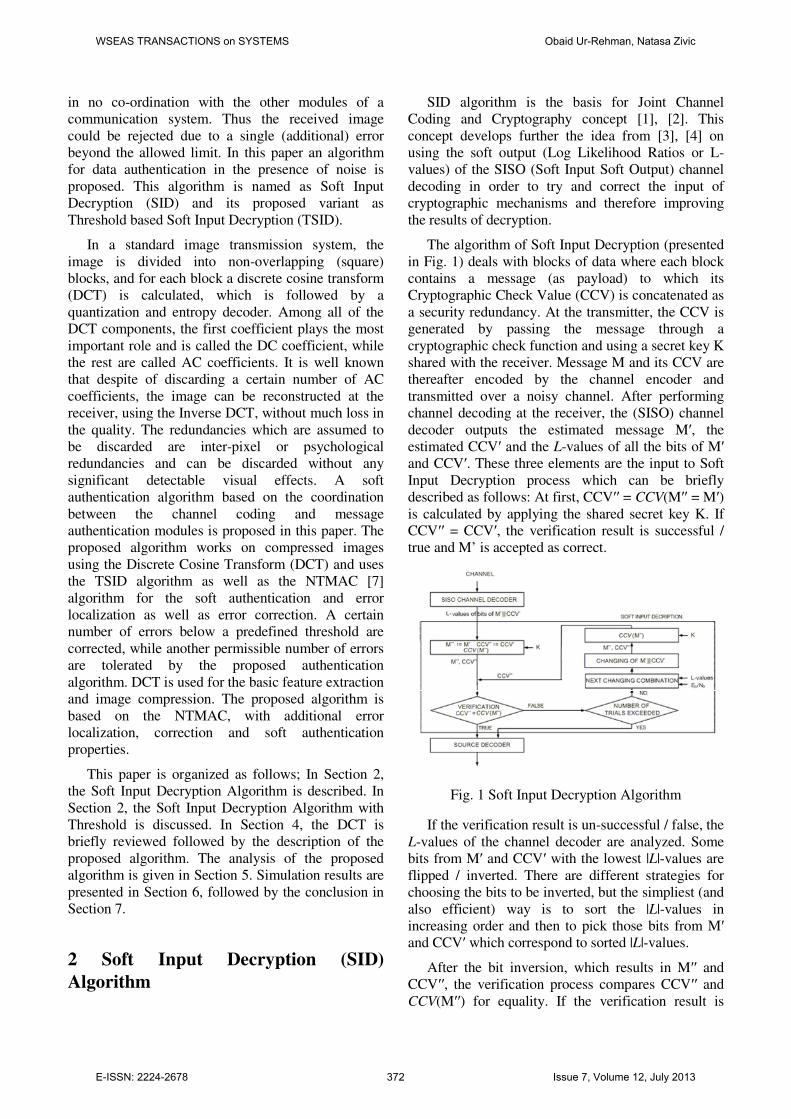
in no co-ordination with the other modules of a
communication system. Thus the received image
could be rejected due to a single (additional) error
beyond the allowed limit. In this paper an algorithm
for data authentication in the presence of noise is
proposed. This algorithm is named as Soft Input
Decryption (SID) and its proposed variant as
Threshold based Soft Input Decryption (TSID).
In a standard image transmission system, the
image is divided into non-overlapping (square)
blocks, and for each block a discrete cosine transform
(DCT) is calculated, which is followed by a
quantization and entropy decoder. Among all of the
DCT components, the first coefficient plays the most
important role and is called the DC coefficient, while
the rest are called AC coefficients. It is well known
that despite of discarding a certain number of AC
coefficients, the image can be reconstructed at the
receiver, using the Inverse DCT, without much loss in
the quality. The redundancies which are assumed to
be discarded are inter-pixel or psychological
redundancies and can be discarded without any
significant detectable visual effects. A soft
authentication algorithm based on the coordination
between the channel coding and message
authentication modules is proposed in this paper. The
proposed algorithm works on compressed images
using the Discrete Cosine Transform (DCT) and uses
the TSID algorithm as well as the NTMAC [7]
algorithm for the soft authentication and error
localization as well as error correction. A certain
number of errors below a predefined threshold are
corrected, while another permissible number of errors
are tolerated by the proposed authentication
algorithm. DCT is used for the basic feature extraction
and image compression. The proposed algorithm is
based on the NTMAC, with additional error
localization, correction and soft authentication
properties.
This paper is organized as follows; In Section 2,
the Soft Input Decryption Algorithm is described. In
Section 2, the Soft Input Decryption Algorithm with
Threshold is discussed. In Section 4, the DCT is
briefly reviewed followed by the description of the
proposed algorithm. The analysis of the proposed
algorithm is given in Section 5. Simulation results are
presented in Section 6, followed by the conclusion in
Section 7.
2 Soft Input Decryption (SID)
Algorithm
SID algorithm is the basis for Joint Channel
Coding and Cryptography concept [1], [2]. This
concept develops further the idea from [3], [4] on
using the soft output (Log Likelihood Ratios or L-
values) of the SISO (Soft Input Soft Output) channel
decoding in order to try and correct the input of
cryptographic mechanisms and therefore improving
the results of decryption.
The algorithm of Soft Input Decryption (presented
in Fig. 1) deals with blocks of data where each block
contains a message (as payload) to which its
Cryptographic Check Value (CCV) is concatenated as
a security redundancy. At the transmitter, the CCV is
generated by passing the message through a
cryptographic check function and using a secret key K
shared with the receiver. Message M and its CCV are
thereafter encoded by the channel encoder and
transmitted over a noisy channel. After performing
channel decoding at the receiver, the (SISO) channel
decoder outputs the estimated message M′, the
estimated CCV′ and the L-values of all the bits of M′
and CCV′. These three elements are the input to Soft
Input Decryption process which can be briefly
described as follows: At first, CCV′′ = CCV(M′′ = M′)
is calculated by applying the shared secret key K. If
CCV′′ = CCV′, the verification result is successful /
true and M’ is accepted as correct.
Fig. 1 Soft Input Decryption Algorithm
If the verification result is un-successful / false, the
L-values of the channel decoder are analyzed. Some
bits from M′ and CCV′ with the lowest |L|-values are
flipped / inverted. There are different strategies for
choosing the bits to be inverted, but the simpliest (and
also efficient) way is to sort the |L|-values in
increasing order and then to pick those bits from M′
and CCV′ which correspond to sorted |L|-values.
After the bit inversion, which results in M′′ and
CCV′′, the verification process compares CCV′′ and
CCV(M′′) for equality. If the verification result is
WSEAS TRANSACTIONS on SYSTEMS Obaid Ur-Rehman, Natasa Zivic
E-ISSN: 2224-2678 372 Issue 7, Volume 12, July 2013

„false” again, another bit or combination of bits is
inverted (corresponding to the binary interpretation of
N-bit counter incremented by 1). This iterative
process continues till either the verification result is
„true” or a threshold number of iterations have been
performed.
The idea of inversion of the least reliable bits
originated from Chase decoding algorithms [3] in
1972, which were the generalization of the GMD
(Generalized Minimum Distance) algorithms from
1966 [4] and improved channel decoding. These
algorithms have been applied to a binary (n, k) linear
block code and are referenced as LRP (Least
Reliability Positions) algorithms. The novelty of SID
is the inversion of bits iteratively for data protected by
cryptographic redundancy with feedback between the
decryptor and the channel decoder, since it gives the
possibility to check whether the inversion iteration
was successful or not (through the process of
verification).
It may happen that a pair of M′′ and CCV′′
generated by the bit inversion passes the verification
although the message M′′ is not equal to the original
message M. The probability of such an event is very
small, which will also be taken in consideration in the
next Section.
In simulations, both message and CCV have the
length of 160 bits. CCV has been calculated using
RIPEMD160 with a key K. Simulations have been
performed using a Convolutional encoder of code rate
r = 1/2 and constraint length m = 2 as the simplest
one, but used very often in theory and practice. BPSK
modulation and an Additive White Gaussian Noise
(AWGN) channel are used together with a SISO
decoder based on the Maximum A-Posteriori (MAP)
algorithm. The MAP decoder was programmed in
such a way, that it supports the output of L-values.
The presentation of the results of the simulations
(Fig. 2) clearly shows obtained benefits and potentials
of SID algorithm. In order to measure the
improvement, a parameter named the Cryptographic
Check Error Rate (CCER) is defined as follows:
CCVsreceivedofnumber
CCVsincorrectofnumberCCER = , (1)
where an incorrect cryptographic check value is
each CCV which didn't pass the verification.
Fig. 2 shows the improvement of CCER with Soft
Input Decryption for the cases that up to 8 of the
lowest |L|-values (graph b) or up to the 16 lowest |L|-
values are used (graph c). Example: CCER of 10-3
at
Eb/N0 ~ 6.2 dB without Soft Input Decryption is the
same as for Eb/N0 ~ 4.2 dB with Soft Input
Decryption, or decreased from 10-1
to 10-3
at Eb/N0 ~
4.2 dB. Using up to 16 of the lowest |L|-values a
coding gain of 2.33 dB can be reached, and CCER >
10-1
without Soft Input Decryption can be reduced
down to CCER < 10-4
at Eb/N0 ~ 4 dB.
Fig. 2 Results of Soft Input Decryption using up to 8
(b) and 16 (c) lowest |L|-values compared to results
without Soft Input Decryption (a)
At this point, a few words need to be said
regarding the L-values and the type of channel
decoder which can be used together with the SID. The
channel decoder is assumed to be SISO (Soft Input
Soft Output). SISO is a concept of channel decoding,
which was originally used in iterative and Turbo
coding, because the (soft) output is fed-back
internally. Soft output of the channel decoder is used
here as the soft input for the cryptographic
verification process (called Soft Input Verification).
Soft output of the channel decoder is usually
expressed as L-value of each output bit u′,
)0(
)1(ln)'(
=
==
uP
uPuL , (2)
L(u′) represents the reliability of the decision made
by the channel decoder, i.e., if the sent bit u was a 1 or
0. The sign of the L-value shows the hard output of bit
u′ (1 or 0) and the magnitude, i.e., |L|, is used as
reliability value of the hard decision. Example: if L is
positive, the hard output is 1, otherwise it is 0. The
higher the |L|, the more reliable is the hard decision
and vice versa: a lower |L| means a less reliable
decision. When the L-Value is equal to 0, the
probability of the correctness of the decision is 0.5.
It is obvious that SID method greatly depends on
the "quality" of L-values, which means that "better
information" on bit reliability will give better results
WSEAS TRANSACTIONS on SYSTEMS Obaid Ur-Rehman, Natasa Zivic
E-ISSN: 2224-2678 373 Issue 7, Volume 12, July 2013

after SID. The decoder which produces L-values need
not to be exclusively of SISO type, but each L-value
provided for each particular bit must, in some way,
represent its reliability. Such a requirement
disqualifies, for example, Viterbi decoding since then,
the produced array of L-values gives the probabilities
of the paths through trellis and not bit reliabilities.
From the other side, there is MAP decoder (used in
simulations) which internally calculates probabilities
of each bit value taking into account the values of all
other bits before and after a particular bit. Having all
these probabilities already obtained by MAP, using
(2) it is easy to get L-values which are suitable for the
use within SID.
MAP is also a SISO decoder, which, besides the
bit array from the output of line decoder (i.e.
demodulator), as input can take the soft information
on the probabilities of demodulated bits as well. It is
important because then MAP has the opportunity to
be used as a part of different more efficient (and more
complex) decoding schemes with feedback. One of
them is Turbo-decoding scheme where two MAP
blocks are coupled over "crossed feedbacks", working
together in an iterative process. In the above
mentioned simulations, the "pure MAP" without
feedback is used, which assumes that all the input
probabilities of demodulated bits (soft input) have
been preset on the value of 0.5.
Having in mind the way on which MAP internally
calculates bit probabilities, one can conclude that for
better results, the length of input bit array (in our case
message M concatenated with its CCV) shouldn't be
too small, since each bit probability (and the decision
based on it) will be calculated using more neighboring
bits. On the other side, the more distant bits have
smaller influence on the calculations and also can add
numerical noise, so it is expected that there is an
optimal length of MAP input array (which is equal to
the length of output array). The obtained results are
also affected by the quality of L-values from the MAP
decoder, which as explained, depends on the lengths
of message and CCV. After all, the resume is that
message and CCV together should have an optimal
length (or close to optimal). In such a case where the
messages are too long (or a continuous data stream is
to be transmitted), they should be fragmented and for
each fragment the CCV should be calculated, so that
all together have more or less optimal length.
3 Soft Input Decryption Using
Threshold
Although it seems that the SID method, especially
in the scenario with a feedback, has exploited the
whole soft information available from the channel
decoder but further improvements of coding gain are
still possible. Since the decryption of CCV is very
sensitive to errors, the verification process need not to
be so “strict” as it used to be. This gives more space
for the SID method, which is now able to choose L-
values more precisely by setting the verification
threshold. Setting the threshold increases the
probability of the false verification (collision), but
even then it is extremely small.
The efficiency of SID method depends on the
obvious factors such as the lengths of the message and
the CCV, the number of bits chosen for inversion and
the Eb/N0 ratio. Some results of many simulations for
different values of these parameters are presented in
the previous Section as well as in [1]. Besides the
mentioned parameters, the “quality” of L-values
produced by channel decoder plays an important role,
which indirectly affects the overall efficiency of the
process involving SID. Naturally, SID works better
with a smaller as compared to a bigger portion of data
which is to be corrected.
One way to decrease the data length used by SID
is to exclude the bits of cryptographic check value
from correction within SID. Namely, if the length of
the message is m and the length of cryptographic
check value is n, SID now considers only m instead of
m+n elements. SID picks N lowest |L|-values and
inverts corresponding bits (only from decoded
message M') in the iterative process of verification.
The above proposed enhancement of SID method
is possible since the cryptographic check value
satisfies the so called avalanche criterion which
assumes that wrong decoded (i.e., reconstructed) CCV
has in average 50% of the bits wrong. This means that
if only one bit from the decoded message M′ is
erroneous, around n/2 bits in CCV′′ will be erroneous
as well. In other words, when a decoded message M′
is incorrect, CCV(M′) must have many wrong bits,
much more (i.e. significantly more) than the decoded
CCV'. So in the case that CCV′′ contains “only a few”
incorrect bits, i.e., when the Hamming distance (HD)
between CCV′ and CCV′′, i.e., HD(CCV', CCV") is
“small enough”, it is obvious that M′ is correct (M′
equals original M) and that the difference between
CCV′ and CCV′′ exists only because of the errors in
CCV′. Hence, during the verification process within
"Thresholded SID" (TSID), there is no need to check
if all the bits from CCV′′ are equal to the
corresponding bits in CCV′, but the criterion for
successful verification would be that d=HD(CCV',
WSEAS TRANSACTIONS on SYSTEMS Obaid Ur-Rehman, Natasa Zivic
E-ISSN: 2224-2678 374 Issue 7, Volume 12, July 2013
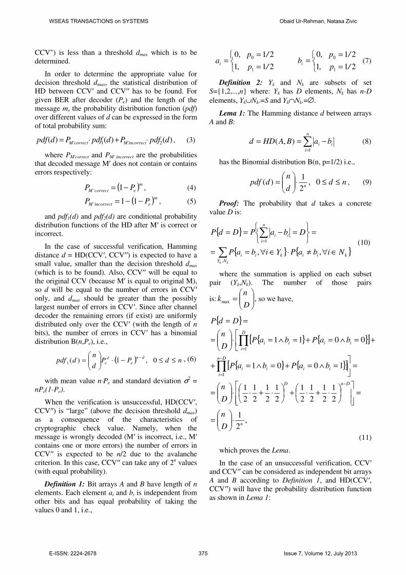
CCV") is less than a threshold dmax which is to be
determined.
In order to determine the appropriate value for
decision threshold dmax, the statistical distribution of
HD between CCV′ and CCV′′ has to be found. For
given BER after decoder (Pe) and the length of the
message m, the probability distribution function (pdf)
over different values of d can be expressed in the form
of total probability sum:
)()()( 2'1' dpdfPdpdfPdpdf incorrectMcorrectM ⋅+⋅= , (3)
where PM'correct and PM' incorrect are the probabilities
that decoded message M′ does not contain or contains
errors respectively:
( )m
ecorrectM PP −= 1' , (4)
( )m
eincorrectM PP −−= 11' , (5)
and pdf1(d) and pdf2(d) are conditional probability
distribution functions of the HD after M′ is correct or
incorrect.
In the case of successful verification, Hamming
distance d = HD(CCV′, CCV′′) is expected to have a
small value, smaller than the decision threshold dmax
(which is to be found). Also, CCV′′ will be equal to
the original CCV (because M′ is equal to original M),
so d will be equal to the number of errors in CCV′
only, and dmax should be greater than the possibly
largest number of errors in CCV′. Since after channel
decoder the remaining errors (if exist) are uniformly
distributed only over the CCV′ (with the length of n
bits), the number of errors in CCV′ has a binomial
distribution B(n,Pe), i.e.,
( ) ndPPd
ndpdf
dn
e
d
e ≤≤−⋅
=
−0 ,1)(1
, (6)
with mean value n⋅Pe and standard deviation σ2 =
nPe(1-Pe).
When the verification is unsuccessful, HD(CCV′,
CCV′′) is “large” (above the decision threshold dmax)
as a consequence of the characteristics of
cryptographic check value. Namely, when the
message is wrongly decoded (M′ is incorrect, i.e., M′
contains one or more errors) the number of errors in
CCV′′ is expected to be n/2 due to the avalanche
criterion. In this case, CCV′′ can take any of 2n values
(with equal probability).
Definition 1: Bit arrays A and B have length of n
elements. Each element ai and bi is independent from
other bits and has equal probability of taking the
values 0 and 1, i.e.,
=
==
=
==
21 ,1
21 ,0
21 ,1
21 ,0
1
0
1
0
/p
/pb
/p
/pa ii (7)
Definition 2: Yk and Nk are subsets of set
S={1,2,...,n} where: Yk has D elements, Nk has n-D
elements, Yk∪Nk.=S and Yk∩Nk.=∅.
Lema 1: The Hamming distance d between arrays
A and B:
∑=
−==n
i
ii baBAHDd1
),( (8)
has the Binomial distribution B(n, p=1/2) i.e.,
ndd
ndpdf
n≤≤⋅
= 0 ,
2
1)( , (9)
Proof: The probability that d takes a concrete
value D is:
{ }
{ } { }∑
∑
∈∀≠⋅∈∀==
=
=−===
kk NY
kiikii
n
i
ii
NibaPYibaP
DbaPDdP
,
1
,,
(10)
where the summation is applied on each subset
pair (Yk,Nk). The number of those pairs
is:
=
D
nkmax , so we have,
{ }
{ } { }[ ]
{ } { }[ ]
,2
1
2
1
2
1
2
1
2
1
2
1
2
1
2
1
2
1
1001
0011
1
1
n
DnD
Dn
i
iiii
D
i
iiii
D
n
D
n
baPbaP
baPbaPD
n
DdP
⋅
=
=
⋅+⋅+
⋅+⋅⋅
=
=
=∧=+=∧=+
+=∧=+=∧=⋅
=
==
−
−
=
=
∏
∏
(11)
which proves the Lema.
In the case of an unsuccessful verification, CCV′
and CCV′′ can be considered as independent bit arrays
A and B according to Definition 1, and HD(CCV′,
CCV′′) will have the probability distribution function
as shown in Lema 1:
WSEAS TRANSACTIONS on SYSTEMS Obaid Ur-Rehman, Natasa Zivic
E-ISSN: 2224-2678 375 Issue 7, Volume 12, July 2013

ndd
ndpdf
n≤≤⋅
= 0 ,
2
1)(2 , (12)
Equation (12) can also be explained in simpler
way. Namely, when the message is not verified, the
expected value of HD(CCV′, CCV′′) is equal to the
expected value of HD between CCV′ and any other
fixed array of bits of the same length. If for
simplicity, we choose an array of bits X = 00...0, the
HD(CCV′, X) will also have Binomial distribution
B(n,p), where p=1/2 since every bit in CCV′ is
expected to be 0 or 1 with equal probability, so the pdf
of HD(CCV′, CCV′′) can be written as in (12).
By combining equations (4), (5), (6) and (12) in
(3), for the parameter values m=160, n=160 and
Pe=0.01, the probability distribution of d = HD(CCV′,
CCV′′) will have the shape as shown in Fig.3. Two
regions are clearly distinguished: the left one for the
case of successfully decoded message (i.e., M = M′)
and the second − when the decoded message M′ is
wrong (i.e., M ≠ M′). It is obvious that the probability
distribution over d is zero for a great range of values
between these regions, which means that the decision
threshold dmax in the process of verification might take
any value from this middle area.
Fig. 3 Probability distribution of d=HD(CCV′,
CCV′′)
The rate of acceptance of decoded and by flipping
corrected messages within verification process will be
greater if the dmax is set to a greater value. The lower
limit of the threshold (dmax_low) can be chosen in
relation to wanted acceptance rate of message, i.e.,
regarding the predefined probability of message
rejecting. In columns 3, 5 and 7 of Table 1 (see
Appendix) the values of dmax_,low are shown for
different lengths of cryptographic check value (n =
160, 128, 64) and message (m = 160, 192, 256) so
that m+n = 320 and for different BERs (depending on
Eb/N0). The criteria for choice of dmax,low was that the
probability of message rejecting (when M′ is correct)
is less than 10-k, i.e.,
kn
dd
corectM
low
dpdfP−
+=
<⋅∑ 10)(1
1'
max_
, (12)
where PM'correct and pdf1(d) are defined in (8) and
(10), and the condition for message to be accepted as
correct is,
max)",'( dCCVCCVHDd ≤= . (13)
By setting the parameter k to an appropriate value,
wanted minimal acceptance rate can be achieved and
the matching values of dmax_low can be calculated from
(12) and (13). The values of dmax_low obtained in this
way are shown in Table I, where each cell contains
four different values: for k = 4, 6, 10 and 15
respectively.
On one hand, greater dmax and higher acceptance
rate of messages means speeding up the verification
process, since the expected number of bit-flipping
iterations leading to successful verification is smaller.
Greater dmax, on the other hand, will increase the
probability of false verification − the event when the
decryptor wrongly decides that a decoded message M′
(or the corrected message M′′ after a number of bit-
flipping iterations) is correct. This happens when
CCV′′, which acts as a random variable (since
calculated from wrong decoded message M′ and the
secret key K), satisfies the condition (7). The
probability of false verification becomes significant
when the value of decision threshold dmax is getting
closer to the region on the right side in Fig.3.
Similarly as by choosing the lower limit, the upper
limit of the threshold (dmax,high) can be found with
regard to the probability of false verification which
can be tolerated. This probability can be also defined
by the use of parameter k, while dmax,high will be the
maximal integer that satisfies the following condition:
k
d
d
incorectM
high
dpdfP −
=
<⋅∑ 10)(max_
0
2' , (14)
(in (3) and (5) are the definitions of PM'incorrect and
pdf2(d)).
Columns 4, 6 and 8 of “Table 1” contain values of
dmax,high calculated from (8) for k=4, 5, 10 and 20
respectively. There is a lot of values within range
[dmax,low+1, dmax,high] which could be taken as the
threshold, for different values of parameters Eb/N0, Pe,
m and n.
Both SID and TSID methods have been simulated
with the message and its CCV / HMAC tag, both of
length of 160 bits. HMAC tag has been calculated
WSEAS TRANSACTIONS on SYSTEMS Obaid Ur-Rehman, Natasa Zivic
E-ISSN: 2224-2678 376 Issue 7, Volume 12, July 2013

using RIPEMID160 hash function. Simulations have
been performed using a Convolutional encoder of
code rate r (= ½) and a constraint length m = 2, BPSK
modulation, AWGN channel and SISO decoding
using MAP algorithm.
The results of simulations are expressed through
Cryptographic Check Error Rate (CCER), already
defined by (1), as the ratio between the number of
incorrect CCVs after (T)SID and the whole number of
simulations for given set of parameters. In both
methods 16 bits with smallest |L|-values were being
flipped, i.e., maximally 216
trials of soft correction (bit
flipping) had been performed in each simulation. The
value of decision threshold within TSID had been set
to 20% of the CCV length dmax= 32.
Fig. 4 Achieved coding gains of SID and SID with
threshold (TSID)
The results are presented in Fig. 4, showing the
achieved coding gain in comparison to standard 1/2
convolutional coding. Using original SID method,
more than 1.4 dB of gain is achieved, while TSID
obtains additional 0.5-0.6 dB.
4 Authentication Of Images Using
TSID And Noise Tolerant MACs
(NTMACs) Based On The Discrete
Cosine Transform
4.1 Introduction
In this Section the application of TSID algorithm
in combination with the Noise Tolerant Message
Authentication Code (NTMAC) is investigated in
image authentication. For images, the basic features
are authenticated rather than authenticating the image
itself. For this purpose, the Discrete Cosine Transform
is used to extract the block by block features and
authenticate the image block-wise. This is also
beneficial for the TSID algorithm, which works well
over small blocks of data as compared to big ones.
4.2 Discrete Cosine Transform in Image
Processing Discrete Cosine Transform is one of the most
widely used techniques in image processing for basic
feature extraction and compression. Its application in
image processing was pioneered in [16]. Due to its
better reconstruction capability, DCT is more suitable
to images than other relevant transforms, such as
Discrete Fourier Transform (DFT). DCT, like other
transforms, tries to eliminate the correlation from
image data. After de-correlation, each transform
coefficient can be encoded independently without
devitalizing the compression efficiency. Many well
known image and video compression standards like
JPEG and MPEG-1/2/4/H.26x, are based on 2-D
DCT.
The Discrete cosine transform of a 2-D vector is
defined as follows [16-18]:
∑∑−
=
−
=
+
+=
1
0
1
0 2
)12(cos
2
)12(cos),(
2)()(),(
N
m
N
n N
n
N
mnmx
NklklX
ππαα
where,
−≤≤
==
11 ,1
0 ,2/1)(
Ni
iiα (15)
It is clear from (15) that the first coefficient (DC)
represents the average intensity of the corresponding
block and contains most of the energy and perceptual
information. Also the inverse of 2-D DCT for l,k = 0,
1, ..., N-1 is defined as follows,
∑∑−
=
−
=
+
+=
1
0
1
0 2
)12(cos
2
)12(cos),(
2)()(),(
N
m
N
n N
n
N
mnmX
Nklklx
ππαα (16)
Besides the general characteristics of DCT which
are defined for every Fourier-like transform, other
properties of DCT like de-correlation, energy
compactness, symmetry and separability make it a
convenient tool for image processing purposes.
4.3 Introduction and Definitions The algorithm introduced in this paper is based on
the DCT transform. It protects the transmitted DCT
components of an image by NTMAC and performs
soft authentication on received (noisy) images. The
algorithm is able to localize errors in the images and
to correct a certain number of them if they are below a
WSEAS TRANSACTIONS on SYSTEMS Obaid Ur-Rehman, Natasa Zivic
E-ISSN: 2224-2678 377 Issue 7, Volume 12, July 2013

certain threshold. The following definition is used in
the description of the proposed algorithm.
Definition 3: Let H´ be the received n-bit MAC
for a transmitted message M. Let M´ be the received
message, H´´ be the MAC recalculated at the receiver
and let d be a small non-negative integer (d << n/2);
then (M´, H´) is said to be d-soft-verified if HD(H´,
H´´ ) ≤ d, where HD is the Hamming Distance
between H´ and H´´.
For the sake of simplicity, let’s assume the image
to be transmitted is N × N pixels. Let m be the block
size such that m|N, where both N and m are integers.
The sender divides the image into m × m-pixel
disjoint blocks (typically m is equal to 8). This is
followed by the calculation of DCT for each block.
4.4 Image Authenticating and Correcting
Weighted Noise Tolerant MAC (IAC-
WNTMAC) IAC-WNTMAC achieves error localization using
the concept of weights. IAC-WNTMAC is based on
NTMAC [7] and identifies the locations of potential
erroneous blocks with a high probability.
The NTMAC algorithm [7] works by splitting a
message / image into smaller components. A MAC is
calculated for each of the smaller components and
truncated to obtain a sub-MAC. The sub-MACs
corresponding to these message components are
concatenated to form the NTMAC. The IAC-
WNTMAC tag calculation can either operate row-
wise or column-wise on the image blocks. It is
assumed here that the tag calculation is done row-
wise. A DCT matrix is obtained for each block in the
source image. Thus there are as many DCT matrices
as the number of blocks in the source image. NTMAC
is calculated based on the DC components of the DCT
matrices taken row-wise. There are N/m such DCT
matrices in each row and therefore N/m DC
components are used to get one NTMAC (against a
row).
The same step is repeated for all the rows, giving
N/m NTMACs. This process is also repeated for the
first minor diagonal after DC coefficient (called as
first minor diagonal for the sake of simplicity) of the
DCT matrices, giving another set of N/m NTMACs.
This produces a total of 2(N/m) MACs, i.e., N/m +
N/m. The usage of NTMAC improves the error
localization, whereas the usage of the NTMAC for the
minor diagonal increases the quality of reconstructed
image at the receiver as explained next. All of these
N/m + N/m NTMAC tags are appended together to
obtain IAC-WNTMAC tag for transmission.
The image I´ and its IAC-WNTMAC´ tag are
received over a noisy channel. The receiver
recalculates IAC-WNTMAC tag on I´ to get IAC-
WNTMAC´´. Now the received IAC-WNTMAC´ tag
is compared with the recalculated IAC-WNTMAC´´
tag. This is done by comparing the corresponding sub-
MACs. If the sub-MACs are d-soft-verified according
to the definition given above, then the DC component
is accepted as authentic and the message block
corresponding to the DC component is declared as
authentic. Otherwise, the block is marked as un-
authentic / suspicious. All the blocks marked as un-
authentic / suspicious will be tried for error correction
using Chase like iterative error correction algorithm
based on the bit reliabilities calculated using the MAP
decoder at the receiver. This iterative error correction
is repeated for the first minor diagonal as well, so that
they can be reconstructed to get a better quality of the
reconstructed image. However, the first minor
diagonal has a lower weight than the DC component.
Lower weight means that the threshold for the
maximum number of iterations used for the recovery
of the first minor diagonal is smaller than the
threshold used for the recovery of the DC component,
i.e., a variation of the EC-WNTMAC [10] is used. If
TiterDC is the iteration threshold used for the error
correction of DC components and TitrFMD is the same
used for the first minor diagonal, then the total
number of iterations are given by,
Titr = TitrDC + TitrFMD (17)
The pseudo-code of the IAC-WNTMAC tag
generation and verification algorithms is given below
for an N × N image. It can be easily extended to the
general case where the image is not square. Also here
weights are assigned based on the DC and the first
minor diagonal elements, which can be easily
extended to other minor diagonals. The notation DC is
self explanatory, whereas MD represents the Minor
Diagonal of the DCT matrix.
Algorithm: IAC-WNTMAC Tag Generation
Algorithm
Inputs:
• Source Image (I)
• Image width / height in pixels (N)
• Block length (m)
Algorithm:
blocks = splitImageIntoBlocks(I, N, m)
for i = 1 to N/m
WSEAS TRANSACTIONS on SYSTEMS Obaid Ur-Rehman, Natasa Zivic
E-ISSN: 2224-2678 378 Issue 7, Volume 12, July 2013

for j = 1 to N/m
DCT = blocksi,j
DC = DCT1,1
subMACDCj = calcSubMAC(DC)
subMACMDj = calcSubMAC(DCT1,2 ||
DCT2,1)
end
subMACDCi = subMACDC1 || … subMACDCN/m
subMACMDi = subMACMD1 || … subMACMDN/m
end
NTMACDC = subMACDC1 || subMACDC2 || … ||
subMACDCN/m
NTMACMD= subMACMD1 || subMACMD2 || … ||
subMACMDN/m
Output:
NTMACDC || NTMACMD
Pseudo code for tag verification at the receiver:
Algorithm: IAC-WNTMAC Tag Verification at the
Receiver
Inputs:
• Received Image (I´)
• Received NTMAC´
• Image width / height (N)
• Block length (m)
• Block LLRs (blockLLRs)
Algorithm:
I´´ = decompressImage(I´)
subMAC´DC = makeDCSubMACs(NTMAC´)
subMAC´MD = makeMDSubMACs(NTMAC´)
dc_LLRs = blockLLRsToDCLLRs(blockLLRs)
md_LLRs = blockLLRsToMDLLRs(blockLLRs)
blocks = makeBlocks(I´´, W, H, m)
for i=1 to N/m
for j=1 to N/m
DCT = blocksi,j
DC = DCT1,1
subMACDCi,j = calcSubMAC(DC)
subMACMDi,j = calcSubMAC(DCT1,2 ||
DCT2,1)
if( HD(subMAC´DCi,j, subMACDCi,j) ≤ d )
performErrorCorrection(DC, DC_LLRsi,j)
end
if( HD(subMAC´MDi,j, subMACMDi,j) ≤ d )
performErrorCorrection(DCT1,2||DCT2,1,
MD_LLRsi,j)
end
end
end
Output: authenticMessageBlocks
Fig. 5 IAC-WNTMAC Transmitter
Fig. 6 IAC-WNTMAC Receiver
B1,1
B2,1
B1,Nb .................
.................
.................
..................
S1,1 ................
................
.................
.................
.................
B2,Nb
BNb,1 BNb,Nb .................
S2,1
S1,2
S2,2
SNb,1 SNb,2
S1,Nb
S1,Nb
SNb,Nb
Bi,j = Image Block
Si,j = sub-MAC of Bi,j
Pi,j = Pixel in a Bi,j
MSB(W, n) = Keep n-Most Significant Bits of W
WNTMAC = NTMACDC + NTMACMD
P1,1 ................. P1,m
P2,1 ................. P2,m
.
.
Pm,1 ............... Pm,m
Bi,j
DC AC1,2 …... AC1,m
AC2,1 ............ AC2,m
.
.
ACm,1 .......... ACm,m
DCT
subMACi,j =
MSB(MAC(DC), n)
NTMACDCi
NTMACDCNb
S1,1 ................
................
.................
.................
.................
S2,1
S1,2
S2,2
SNb,1 SNb,2
S1,Nb
S1,Nb
SNb,Nb
NTMACMDi
NTMACMDNb
subMACi,j =
MSB(MAC(AC1,2||AC2,1), n)
Calculate sub-MACs on DC and
first minor diagonal‘s AC
components
DC AC1,2 AC2,1 ............ AC1,5 AC5,1 .......... AC5,5
Compress
Compressed Block
WNTMAC
NTMAC‘MDN
NTMAC‘DCNb
Yes
B‘1,1
B‘2,1
B‘1,Nb .................
.................
.................
..................
S‘1,1 ................
................
.................
.................
.................
B‘2,Nb
B‘Nb,
1
B‘Nb,Nb .................
S‘2,1
S‘1,2
S‘2,2
S‘Nb,1 S‘Nb,
S‘1,1
S‘1,1
S‘Nb,N
DC’ AC’1,2........... 0
AC’2,1 ................. 0
.
.
0 0 0............... 0
B‘i,j
DC’ AC’1,2 … AC’1,m
AC’2,1 ...........AC’2,m
.
.
AC’m,1 ........ AC’m,m
IDCT
NTMAC‘DCi
S‘1,1 ................
................
.................
.................
S‘2,1
S‘1,2
S‘2,2
S‘Nb,2
S‘1,1
S‘1,1
S‘Nb,Nb
NTMAC‘MD
subMACi,j =
MSB(MAC(DC’), n)
Perform Iterative Decoding for
Soft Verification of Block Bi,j
Received Image: I‘
Received WNTMAC (WNTMAC‘): NTMAC‘DC + NTMAC’MD
Si,j
HD(subMACi,j
, Si,j) ≤ dmax
No
Mark Block as Authentic
LLRs from Channel
Decoder
S‘Nb,1 .................
WSEAS TRANSACTIONS on SYSTEMS Obaid Ur-Rehman, Natasa Zivic
E-ISSN: 2224-2678 379 Issue 7, Volume 12, July 2013

5 Analysis of the proposed Algorithm IAC-WNTMAC algorithm is a variant of
WNTMAC given in [10]. Therefore the analysis of
the IAC-WNTMAC algorithm is based on
WNTMAC. It is assumed that an ideal n-bit MAC (n
≥ 256) algorithm is used for each row and each
column of concatenated selected DCT elements of
the blocks of an image. The total number of
concatenated DC coefficients is (N/m)2 of k-bit each.
Let the bit error rate of the channel be denoted as
BER.
5.1 Performance Study d-soft-verification is successful, if the difference
between the received MAC and the recalculated one
is not greater than the threshold value. Two types of
errors can exist: “false rejection” (correct image is
discarded) and “false acceptance” (wrong image is
accepted).
The probability of a false rejection of the whole
image (PFR) depends on the policy of the application
and the nature of the image blocks. False rejection is
not as bad as false acceptance, which causes
communication overhead and reduces the efficiency
and therefore the security. Therefore the probability
of false acceptance will be discussed.
False acceptance happens when there are error(s)
in the received image I´, but the received and
recalculated tag pair is d-soft-verified. The
probability of false acceptance on the block level is:
[ ]2
0
)1()1(1)(
−
−−= ∑
=
−d
i
inik
FA BERBERi
nBERBlockP
(18)
5.2 Security Considerations The most important integrity threat against data is
message substitution and forgery. It refers to any
attempt for adding, removing and manipulating
objects into data in order to fool the receiver to accept
the wrong message. This threat in image data can lead
to image tampering.
The algorithms introduced in this paper are based
on the standard ideal MAC, so the generic attacks on
MACs are considered as potential threats. As in the
given approaches, the algorithms may tolerate a
modest number of error(s) as a consequence of soft
verification. The security strength is decreased
generally compared to hard authentication MAC
schemes by allowing near collisions. This drawback is
compensated in both approaches. In the first one each
DCT element is supported by two MACs instead of
one MAC and the attacker has to forge DCT elements
in such a way that both row and column MACs
become d-soft-verified. In the second algorithm, the
attacker has even more difficult task, the forgery
attack requires forgery on protected DC and AC
coefficients so that IAC-WNTMAC authentication on
both selected DC and AC coefficients becomes
successful.
A common approach for approximating the
required complexity (data/time) for forgery attack on
MACs is given by a “birthday paradox” which is
based on finding collisions. In case of soft
authentication, the attacker attempts to launch a near-
collision attack [19]. Near-collision refers to any
message pair whose MACs differ only in few bits
from each other. By extending the birthday paradox to
the introduced soft verification scheme with threshold
d, it is expected to have a near collision (with at most
d-bit differences) with the data complexity (C) of,
∑=
=
d
i
n
i
nC
0
2
2
2 (19)
In the presented algorithms, the minimum MAC
length used to protect row and columns of DC
coefficients is 256 bits. The threshold value is set in
such a way that the probability of events like false
acceptance and false rejection remains significantly
low. There are other experimental methods to find a
convenient safe threshold zone through image
processing techniques. It can be easily concluded that
the security strength compensated by double length
of the MAC is much larger than the required security
strength of a standard MAC, for low threshold
values. The security of the second approach is even
higher due to secret partitioning.
6 Simulation Results The simulation results are presented for the
proposed algorithm using image transmission over
AWGN channel with BPSK modulation. The results
are given in the presence of rate 1/3 Turbo Codes. The
extrinsic Log Likelihood Ratios (LLRs) produced by
the decoder for Convolutional Turbo Codes (CTC) are
used for bit reliabilities values.
The source image is a grayscale image of 128 ×
128 pixels (each pixel of 8 bits). The image is split
into 8 × 8 pixel non-overlapping blocks, giving a total
of 16 × 16 blocks. DCT for each of these blocks is
calculated and the DC components of the DCT sub-
matrices are protected using the corresponding MACs
WSEAS TRANSACTIONS on SYSTEMS Obaid Ur-Rehman, Natasa Zivic
E-ISSN: 2224-2678 380 Issue 7, Volume 12, July 2013

as explained earlier. Each element in the DCT
matrices requires 2 octets. If the original image is
transmitted using the standard MAC based protection,
then either the whole image will be authentic or non-
authentic and so it will either be accepted or
discarded. HMAC-SHA-256 is used as the MAC in
the simulations, thus in total 128 × 128 × 8 bits of
image data plus 256 bits of MAC needs to be
transmitted, which is equal to 131328 bits in total.
Using IAC-WNTMAC, the number of data bits
transmitted is calculated as follows. Each WNTMAC
tag is 256 bits long. Thus, 256 bits for each of the DC
components in the 16 rows as well as another 256 bits
for the first minor diagonals for each row are used.
Thus 256 × 16 × 2 = 8192 bits of WNTMAC tags are
transmitted along the 61440 bits of the data. This is
equal to 53% of the whole data transmitted in the
standard MAC tag based image transmission.
Each figure shown in the following sub-sections is
divided into five constituent sub-images. First, the
source image is shown followed by the received
image. In the next sub-image, the suspicious block
positions (identified through the proposed algorithms)
are highlighted in white followed by these suspicious
blocks highlighted in the received image. Finally, the
resultant image is shown, which is obtained by
applying the proposed error correction algorithm over
the erroneous image based on the localized errors.
6.1 Simulation Results for IAC-WNTMAC Images protected using IAC-WNTMACs have
better error localization capabilities and so they can be
reconstructed in a better manner as compared to the
previous algorithm. The simulation results are
presented in Fig. 7.
Fig. 7 IAC-WNTMAC at SNR 2.5 with Turbo Codes
of rate-1/3
6.2 Image Error Rate (IER) IER for both the algorithms is shown in Fig 8 at
different values of Eb/N0. The curves represent the
IER in the presence of a standard MAC tag based
protection scheme and then in the presence of IAC-
WNTMAC. Fig. 4 shows that IAC-WNTMAC
achieves a coding gain of 1.2 dB at IER of 10-4
. Its
performance is due to dual error protection and
recovery using weighted NTMAC.
7 Conclusion An algorithm for approximate data authentication
(SID) is presented first. This is extended further to
TSID which more efficiently perform authentication
by iteratively considering only the data part in
authentication and doing a threshold number of
comparisons till the match criteria is satisfied. Both
the algorithms fall into the category of fuzzy
authentication algorithms. The application of TSID
together with the NTMAC using DCT is
demonstrated in image authentication. Thus an
algorithm for soft authentication, error localization
and correction of images is presented. Soft
authentication is performed using the standard MAC
together with the threshold value. The main property
of the algorithms is its ability of error localization and
correction without compromise of security, which is
shown in the analysis. Simulation results showing the
high error recovery as well as relatively accurate error
localization validate the theoretical analysis. In future
it would be interesting to extend the proposed work
by combining it with artificial intelligence based
cooperative learning strategies, e.g., the one proposed
in [20]. It is expected to get better content based
image retrieval results using such approaches.
Fig. 8 IER over AWGN channel with BPSK
modulation using Turbo codes of rate-1/3
WSEAS TRANSACTIONS on SYSTEMS Obaid Ur-Rehman, Natasa Zivic
E-ISSN: 2224-2678 381 Issue 7, Volume 12, July 2013

References:
[1] N. Zivic, Joint Channel Coding and
Cryptography, Shaker Verlag, Aachen (2008).
[2] C. Ruland, N. Zivic, Soft Input Decryption, 4th
Turbocode Conference, 6th Source and
Channel Code Conference, VDE/IEEE,
Munich, Apr 2006
[3] D. Chase, A Class of Algorithms for Decoding
Block Codes with Channel Measurement
Information, IEEE Trans. Inform. Theory, IT-
18, pp. 170-182, Jan 1972
[4] G. D. Jr. Forney, Generalized Minimum
Distance Decoding, IEEE Trans. Inform.
Theory, IT-12, pp. 125-131, Apr 1966
[5] R. Gravemen, L. Xie, and G. R. Arce,
Approximate image message authentication
codes, in Proc. 4th Annu. Symp. Advanced
Telecommunications and Information
Distribution Research Program, College Park,
MD, 2000.
[6] R. Graveman and K. Fu, Approximate message
authentication codes, in Proc. 3rd
Annual Fed
lab Symp. Advanced Telecommunications /
Information Distribution, vol. 1, College Park,
MD, Feb 1999.
[7] C. Boncelet, The NTMAC for authentication
of noisy messages, IEEE Trans. Info. Forensics
and Security, vol. 1, no. 1, pp. 35-42, Mar
2006.
[8] D. Onien, R. Safavi-Naini, P. Nickolas and Y.
Desmedt, Unconditionally secure approximate
message authentication, in Proc. The Second
International Workshop on Coding and
Cryptology, Springer, 2009.
[9] R. Ge, G. R. Arce and G. D. Crescenzo,
Approximate message authentication codes for
N-ary alphabets, IEEE Transactions on
Information Forensics and Security, vol. 1, no.
1, 2006.
[10] O. Ur-Rehman, N. Zivic, S. Amir Hossein A.
E. Tabatabaei, C. Ruland, Error Correcting and
Weighted Noise Tolerant Message
Authentication Codes, 5th Int. Conference on
Signal Processing and Communication
Systems (ICSPCS) / IEEE Conference, Hawaii,
USA, Dec 2011.
[11] N. Zivic, M. Flanagan, On Joint Cryptographic
Verification and Channel Decoding via the
Maximum Likelihood Criterion, IEEE Comm.
Letters, vol. 6, no. 5, pp. 717-719, May 2012.
[12] O. Ur-Rehman, A. Tabatabaei, N. Zivic, C.
Ruland, Soft Authentication and Correction of
Images, 9th International ITG Conference on
Systems, Communications and Coding (SCC
2013), Jan 2013, Munich, Germany.
[13] L. Zhang, L. Xi, B. Zhou, Image Retrieval
Method Based on Entropy and Fractal Coding,
WSEAS Transaction on Systems, issue 4, vol.
7, Apr 2008.
[14] C. Aviles-Cruz, A. Ferreyra-Ramirez, J. J.
Ocampo-Hidalgo, I. Vazquez-Alvarez,
Structured-Image Retrieval invariant to
rotation, scaling and translation, WSEAS
Transaction on Systems, issue 8, vol. 8, Aug
2009.
[15] N. Doukas, Low Color-Depth Image
Encryption Scheme for use in COTS
Smartphones, WSEAS Transaction on
Systems, issue 9, vol. 11, Sep 2012.
[16] A. Watson, Image compression using Discret
Cosine Transform, Mathematical Journal,
vol.1, no. 4, pp. 81-88, 1994.
[17] N. Ahmed, T. Natarajan, and K. R. Rao,
Discrete Cosine Transform, IEEE Trans.
Computers, vol. C-23, pp. 90-93, Jan 1974.
[18] P. Yip, and K. R. Rao, Fast Decimation-in-
Time Algorithms for a Family of Discrete Sine
and Cosine Transforms, Circuits, Systems and
Signal Processing, Vol. 3, pp. 387-408, 1984.
[19] B. Preneel, P. C. van Oorschot, MDx-MAC
and building fast MACs, from hash
functions, Proc. CRYPTO 1995, LNCS 963,
Springer-Verlag, pp. 1-14, 1995.
[20] F. Neri, Cooperative evolutive concept
learning: an empirical study, WSEAS
Transaction on Information Science and
Applications,WSEAS Press (Wisconsin, USA),
issue 5, vol. 2, pp. 559-563, May 2005.
WSEAS TRANSACTIONS on SYSTEMS Obaid Ur-Rehman, Natasa Zivic
E-ISSN: 2224-2678 382 Issue 7, Volume 12, July 2013

Appendix
Table 1
Upper and Lower Limits of the Decision Threshold
Eb/N
0
[dB]
Pe
n = 160 , m=160 n = 128 , m=192 n = 64 , m=256
dmax_low
(k = 4, 6, 10, 15) dmax_high
(k = 4, 5, 10, 20)
dmax_low (k = 4, 6, 10, 15)
dmax_high (k = 4, 5, 10, 20)
dmax_low (k = 4, 6, 10, 15)
dmax_high (k = 4, 5, 10, 20)
1 0.036 11, 15, 22, 29 56, 52, 40, 23 7, 12, 19, 25 42, 39, 28, 14 0, 6, 12, 17 16, 14, 7, -
1.5 0.0234 10, 13, 19, 25 56, 52, 40, 23 8, 11, 17, 22 42, 39, 28, 14 4, 7, 11, 16 16, 14, 7, -
2 0.0149 8, 11, 16, 21 56, 52 ,40, 23 7, 10, 14, 19 42, 39, 28, 14 4, 7, 10, 14 16, 14, 7, -
2.5 0.00681 6, 8, 12, 16 56, 53, 40, 23 4, 7, 11, 15 43, 40, 28, 14 4, 5, 9, 12 17, 14, 7, -
3 0.00376 5, 7, 10, 14 57, 53, 40, 24 4, 6, 9, 13 43, 40, 29, 14 3, 5, 7, 10 17, 15, 7, -
3.5 0.00142 3, 5, 7, 10 58, 55, 41, 24 3, 5, 7, 10 44, 41, 29, 14 2, 4, 6, 8 18, 15, 8, -
4 0.00037 2, 3, 5, 8 61, 57, 42, 25 2, 3, 5, 7 46, 43, 30, 15 2, 3, 4, 6 19, 16, 8, -
4.5 0.00024 2, 3, 5, 7 61, 57, 43, 25 2, 3, 5, 7 47, 43, 31, 15 2, 2, 4, 6 19, 17, 8, -
5 0.00012 2, 3, 4, 6 63, 58, 43, 26 2, 2, 4, 6 48, 44, 31, 16 1, 2, 4, 5 20, 18, 9, -
WSEAS TRANSACTIONS on SYSTEMS Obaid Ur-Rehman, Natasa Zivic
E-ISSN: 2224-2678 383 Issue 7, Volume 12, July 2013