An introduction tothe normalized Laplacian

Steve ButlerIowa State University

MathButler.org

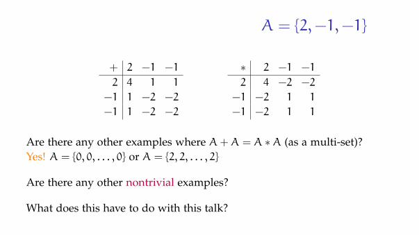
A = {2,−1,−1}

+ 2 −1 −1

2 4 1 1

−1 1 −2 −2

−1 1 −2 −2

∗ 2 −1 −1

2 4 −2 −2

−1 −2 1 1

−1 −2 1 1

Are there any other examples where A+A = A ∗A (as a multi-set)?Yes! A = {0, 0, . . . , 0} or A = {2, 2, . . . , 2}

Are there any other nontrivial examples?

What does this have to do with this talk?

Graphs are collections of objects(vertices) and relations betweenthem (edges).

1

2

3

4

Graphs are very universal andcan model just about everything.

Matrices are arrays of numberswith benefits.

A =

0 1 1 1

1 0 1 0

1 1 0 0

1 0 0 0

Example: eigenvalues are λwhere for some x 6= 0 we haveAx = λx.

{2.17..., 0.31...,−1,−1.48...}

Graphs are collections of objects(vertices) and relations betweenthem (edges).

1

2

3

4

Graphs are very universal andcan model just about everything.

Matrices are arrays of numberswith benefits.

A =

0 1 1 1

1 0 1 0

1 1 0 0

1 0 0 0

Example: eigenvalues are λwhere for some x 6= 0 we haveAx = λx.

{2.17..., 0.31...,−1,−1.48...}

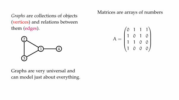
Graphs are collections of objects(vertices) and relations betweenthem (edges).

1

2

3

4

Graphs are very universal andcan model just about everything.

Matrices are arrays of numberswith benefits.

A =

0 1 1 1

1 0 1 0

1 1 0 0

1 0 0 0

Example: eigenvalues are λwhere for some x 6= 0 we haveAx = λx.

{2.17..., 0.31...,−1,−1.48...}

GRAPH ←→ MATRIX −→ EIGENVALUES←−Spectral Graph TheoryWhat are relationships between the structure of a given graph and theeigenvalues of a matrix associated with the graph.

Common matrices

• Adjacency, A: Matrix indicates which vertices are adjacent.Eigenvalues can count closed walks, so can count edges and testbipartite-ness.

• Laplacian, L = D−A: Derived from signed incidence matrix, ispositive semi-definite. Eigenvalues can count edges and number ofcomponents.

• Signless Laplacian, Q = D+A: Derived from unsigned incidencematrix, is positive semi-definite. Eigenvalues can count edges andnumber of bipartite components.

Little less common matrix

• Normalized Laplacian, L “ = ”D−1/2(D−A)D−1/2 : Normalizes theLaplacian matrix, and is tied to the probability transition matrix.• Eigenvalues lie in the interval [0, 2].• Multiplicity of 0 is number of components.• Multiplicity of 2 is number of bipartite components.• Tests for bipartite-ness.• Cannot always detect number of edges.

Summarizing

bip. # comp. # bip. comp. # edges

A YES no no YESL no YES no YESQ no no YES YESL YES YES YES no

Cospectral pairs

Cospectral for A Cospectral for L

Cospectral for Q Cospectral for L

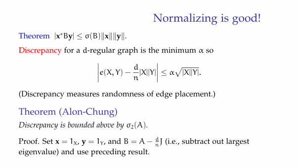
Normalizing is good!Theorem |x∗By| ≤ σ(B)‖x‖‖y‖.

Discrepancy for a d-regular graph is the minimum α so∣∣∣∣e(X, Y) − d

n|X||Y|

∣∣∣∣ ≤ α√|X||Y|.

(Discrepancy measures randomness of edge placement.)

Theorem (Alon-Chung)Discrepancy is bounded above by σ2(A).

Proof. Set x = 1X, y = 1Y , and B = A− dnJ (i.e., subtract out largest

eigenvalue) and use preceding result.

Normalizing is good!

What about non-regular graphs?funnycatpix.com google.com

A has a vertex-centric measure of size. L has an edge-centric measure ofsize (vol(X) =

∑v∈X dv).

Theorem (Chung) For G a graph and X, Y ⊆ V :∣∣∣∣e(X, Y) − vol(X)vol(Y)vol(G)

∣∣∣∣ ≤ σ2(D−1/2AD−1/2)√

vol(X)vol(Y).

Proof. Set x = D1/21X, y = D1/21Y , and B = D−1/2AD−1/2 − 1vol(G)D

1/2JD1/2

(i.e., subtract out largest eigenvalue) and use preceding result.

Using weighted graphs

Let w(u, v) be the weight of the edge between u and v andd(u) =

∑vw(u, v). If we let Au,v = w(u, v) and D(u, u) = d(u), then

L = D−1/2(D−A)D−1/2.

PropositionLet G be a weighted graph and αG the weighted graph resulting fromscaling the weight of each edge by α. Then LG = LαG.

Proof: Scaling terms cancel out by the normalization.

Harmonic eigenvectors

If Ay = µy, then at each vertex t we have∑v

w(t, v)y(v) = µy(t).

Let Lx = λx and let x = D1/2y (y is known as the harmonic eigenvector).Then (D−A)y = λy, or Ay = (1− λ)Dy, or at each vertex t we have∑

v

w(t, v)y(v) = (1− λ)d(t)y(t).

1 is harmonic eigenvector for λ = 0. All other harmonic eigenvectors ysatisfy

∑d(u)y(u) = 0.

Graph operationsThe Cartesian product of G and H, denoted G�H, the tensor product of Gand H, denoted G×H, and the strong product of G and H, denoted G�H,all have vertex set {(a, b) : a ∈ V(G), b ∈ V(H)} and edge sets respectivelyas follows:

E(G�H) ={{(a, b), (c, d)} : a=c and b∼d; or a∼c and b=d

}E(G×H) =

{{(a, b), (c, d)} : a∼c and b∼d

}E(G�H) = E(G�H) ∪ E(G×H).

The join of G and H, denoted G∨H, is the graph formed by taking thedisjoint union of G and H and then adding an edge between every vertexin G and every vertex in H.

L and graph operationsPropositionThere is no way to determine the spectrum of L for the graphs G�H,G�H or G∨H by only knowing the spectrum of L of G and H.

(a) K2,2 �K2 (b) K1,3 �K2 (c) K2,2 �K2

(d) K1,3 � K2 (e) K2,2 ∨K2 (f) K1,3∨K2

L and graph operations

If G and H are regular then we can easily compute eigenvalues of G�Hand G�H using known facts about adjacency matrix. (For regular graphswe can easily go from the spectrum of one matrix to another.)

TheoremEigenvalues of G×H are

{λ+ µ− λµ

}where λ ranges over all eigenvalues of G

and µ ranges over all eigenvalues of H.

L and joins

TheoremLet G be an r-regular graph on n vertices with eigenvalues {λi} and let H be ans-regular graph on m vertices with eigenvalues {θj}. Then the eigenvalues ofG∨H are {

0, 2−r

m+ r−

s

n+ s

}∪{m+ rλim+ r

}∪{n+ sθjn+ s

}.

General ideaWhen a “regular” subgraph cones to the rest of the graph, we can extracteigenvalues from the subgraph and then collapse it to a vertex.

Twin vertices

In a weighted graph, two (non-adjacent) vertices u and v are twins if forevery vertex x

w(u, x) = w(v, x).

(In simple graphs, this translates as having the same neighbors.)

u v w

Über verticesIn a weighted graph a pair of twins can be used to construct (harmonic)eigenvector for eigenvalue 1. Suppose that u and v are twins then

y = 1u − 1v

satisfies at each vertex t∑v

w(t, v)y(v) = 0 = (1− 1)d(t)y(t).

ObservationRemaining eigenvectors have same values at u and v. So treat u and v as asingle über-vertex uv (edge weights summed).

Collapsing twins

• A set of k mutual twins will contribute 1 to the spectrum k− 1 times.We then “collapse” the set of k vertices into a single über-vertex andappropriately adjust the edge weights.

• After collapsing each set of twins we now have a weighted graph andthe remaining eigenvalues are found using this smaller graph.

TheoremIf two graphs collapse to graphs which differ by scaling and in each graphwe removed the same number of “twins”, then the graphs are cospectral.

Example

33

3

33

3

44

4

44

4

Another example

3

66

3

3 3

4

48

2

4 2

1836

18

99

9

1632

16

88

8

Cospectral with subgraph!

With differing number of edges it is theoretically possible to be cospectralwith a subgraph.

×(k+ 1)

×k ×k

×(k+ 1)

×k ×k

After removing twins

k k

k+ 1 k+ 1

1

k2

k k

k+ 1 k+ 1

1

Not just simple rescaling!

Characteristic polynomial for both graphs is:

x5 −6k2 + 8k+ 3

4(k+ 1)2x3 −

1

4(k+ 1)x2 +

k(2k+ 1)

4(k+ 1)2x

A construction

For any circular word in P and C we can form a graph by gluing in acircular chain P4’s and C4’s. For example PPCCPPPC and CCPPCCCP are:

Theorem (B-Heysse) Changing all P↔C does not effect the spectrum of L

Kemeny’s constant and L

Kemeny’s constant, denoted K(G), is the expected first passage time froman unknown starting point to an unknown destination point.

Theorem (Levene-Loizou)If ρn−1 ≤ · · · ≤ ρ1 < ρ0 = 1 are eigenvalues of transition matrix D−1A then

K(G) =

n−1∑i=1

1

1− ρi.

If 0 = λ0 < λ1 ≤ · · · ≤ λn−1 are eigenvalues of L then K(G) =n−1∑i=1

1

λi= −

c2

c1

where pL(t) = tn + · · ·+ c2t2 + c1t.

Kemeny’s constant and L

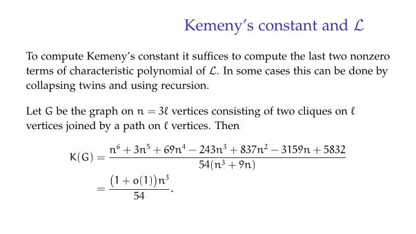
To compute Kemeny’s constant it suffices to compute the last two nonzeroterms of characteristic polynomial of L. In some cases this can be done bycollapsing twins and using recursion.

Let G be the graph on n = 3` vertices consisting of two cliques on `vertices joined by a path on ` vertices. Then

K(G) =n6 + 3n5 + 69n4 − 243n3 + 837n2 − 3159n+ 5832

54(n3 + 9n)

=

(1+ o(1)

)n3

54.

Still much to do!

Many things are still unknown about the normalized Laplacian. Inaddition to having differing number of edges, it is possible for regulargraphs to be cospectral with non-regular graphs.

A+A = A ∗A{2,

√5− 1

2,

√5− 1

2,−√5− 1

2,−√5− 1

2

}• For the adjacency matrix the eigenvalues of G�G are all possible

sums of eigenvalues.

• For the adjacency matrix the eigenvalues of G×G are all possibleproducts of eigenvalues.

• C2k+1�C2k+1 ∼= C2k+1 × C2k+1.• Take A to be the eigenvalues of the adjacency matrix for an odd cycle:

A =

{2 cos

2πk

2k+ 1: k = 0, 1, . . . , 2k

}.

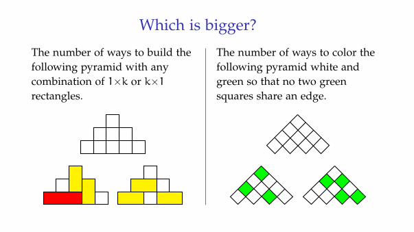
Which is bigger? They’re equal!

The number of ways to build thefollowing pyramid with anycombination of 1×k or k×1rectangles.

The number of ways to color thefollowing pyramid white andgreen so that no two greensquares share an edge.

Which is bigger? They’re equal!

The number of ways to build thefollowing pyramid with anycombination of 1×k or k×1rectangles.

The number of ways to color thefollowing pyramid white andgreen so that no two greensquares share an edge.

Which is bigger? They’re equal!

The number of ways to build thefollowing pyramid with anycombination of 1×k or k×1rectangles.

The number of ways to color thefollowing pyramid white andgreen so that no two greensquares share an edge.