An introduction to persistent homology

MUSTAFA HAJIJ

Part I : Scalar Functions

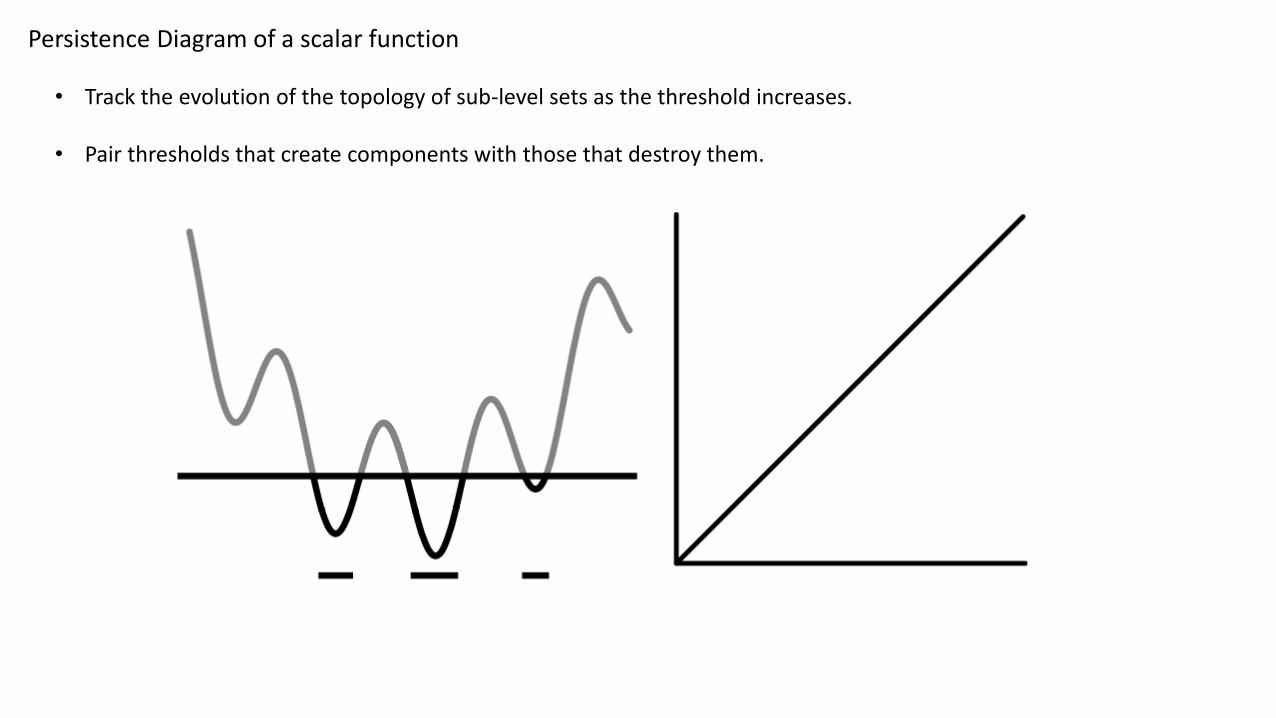
Persistence Diagram of a scalar function

• Track the evolution of the topology of sub-level sets as the threshold increases.

• Pair thresholds that create components with those that destroy them.

Persistence Diagram of a scalar function

• Track the evolution of the topology of sub-level sets as the threshold increases.

• Pair thresholds that create components with those that destroy them.

Persistence Diagram of a scalar function

• Track the evolution of the topology of sub-level sets as the threshold increases.

• Pair thresholds that create components with those that destroy them.

Persistence Diagram of a scalar function

• Track the evolution of the topology of sub-level sets as the threshold increases.

• Pair thresholds that create components with those that destroy them.

Persistence Diagram of a scalar function

• Track the evolution of the topology of sub-level sets as the threshold increases.

• Pair thresholds that create components with those that destroy them.

Persistence Diagram of a scalar function

• Track the evolution of the topology of sub-level sets as the threshold increases.

• Pair thresholds that create components with those that destroy them.

Persistence Diagram of a scalar function

• Track the evolution of the topology of sub-level sets as the threshold increases.

• Pair thresholds that create components with those that destroy them.

Persistence Diagram of a scalar function

• Track the evolution of the topology of sub-level sets as the threshold increases.

• Pair thresholds that create components with those that destroy them.

Persistence Diagram of a scalar function

• Track the evolution of the topology of sub-level sets as the threshold increases.

• Pair thresholds that create components with those that destroy them.

Another example

Persistence Diagram of a scalar function

The pairing algorithm

• Input : a discrete sample 𝑃 = {𝑝1 = (𝑥1, 𝑦1), … , 𝑝𝑛 = (𝑥𝑛, 𝑦𝑛)} representing a scalar function f.

• A collection of paired points.

1. Initiate an empty UnionFind U.2. Sort 𝑃 with respect the y values.3. For every 𝑝𝑖 = 𝑥𝑖 , 𝑦𝑖 𝑖𝑛 𝑃:

1. If 𝑦𝑖−1 > 𝑦𝑖 and 𝑦𝑖+1 > 𝑦𝑖 𝑡ℎ𝑒𝑛 ∶1. U.add(i)2. Set the birth of i to 𝑦𝑖

2. Else if 𝑦𝑖−1 < 𝑦𝑖 and 𝑦𝑖+1 < 𝑦𝑖 𝑡ℎ𝑒𝑛:1. c=U.get(i-1)2. d=U.get(i+1)3. U.merge(c,d)4. Pair 𝑖 with c or d (choose the one that was born later)

3. Else:1. c=U.get(i-1)2. U(c):=U(c) union i

Part II : Point CloudsIntroduction to VR and Cech complexes

Nerve of a topological space

Given a set of points P sampled from a space X, how

can we recover the topological features of the original

space X from the point cloud P?

Nerve of a topological space

We want a discretized structure that capture the shape of the

space and we want a reasonable way that is subtle enough to

measure this shape.

Nerve of a topological space

Čech complex

For each subset Y of X, form a -ball around each point in Y, and include Y as a simplex

,of dimension |Y|, if there is a common point contained in all of the balls in Y.

Given a point cloud X in some metric space and a number , the Čech complex

is the simplicial complex whose simplices are constructed as follows :

The Cech complex approximates the topological space

The homotopy type of and are the same. Theorem:

The Cech complex approximates the topological space

The homotopy type of and are the same. Theorem:

Čech complex size

For each subset Y of X, form a -ball around each point in Y, and include Y as a simplex

,of dimension |Y|, if there is a common point contained in all of the balls in Y.

What is the computational problem in constructing a Čech complex?

If we have a point cloud set X of size 40 then we have to check all subsets of X of size 40. This is 2^{40}.

Very slow!

Vietoris–Rips complex

Let X is a subset of a metric space d and let . The Vietoris–Rips complex is constructed as follows :

This complex is denoted by

Čech complex and VR complex

Comparison between the two complexes :

Note that the VR complex does not

necessarily have the same homotopy

type of the space of the union of ball.

Čech complex and VR complex

What is the relation between the Čech complex and VR complex ?

Čech complex and VR complex

What is the relation between the Čech complex and VR complex ?

So the VR complex forms a good approximation of the Čech complex.

Measuring the shape

Now that we have a good representation of the space, how do we

“measure” it?

Measuring the shape

Now that we have a good representation of the space, how do we

“measure” it?Answering this question can be

done using a tool in topology

called Homology.

Measuring the shape

Now that we have a good representation of the space, how do we

“measure” it?Answering this question can be

done using a tool in topology

called Homology.

Homology is computable via

linear algebra

Measuring the shape

Now that we have a good representation of the space, how do we

“measure” it?Answering this question can be

done using a tool in topology

called Homology.

Homology is computable via

linear algebra

Roughly speaking, homology counts :

• The number of connected components,

• The number of cycles

• The Number o voids in a space

Measuring the shape

Now that we have a good representation of the space, how do we

“measure” it?Answering this question can be

done using a tool in topology

called Homology.

Homology is computable via

linear algebra

Roughly speaking, homology counts :

• The number of connected components,

• The number of cycles

• The Number o voids in a space

This space here has 1 connected component

and 3 cycles

What size do we consider?

We will come back

to this question

later.

Remarks on computing the Vietoris–Rips complex

Given a point cloud X we want to construct a filtration F using VR construction.

Given a point cloud X we want to construct a filtration F using VR construction.

We will utilize the following easy fact :

Remarks on computing the Vietoris–Rips complex

This allows us in practice to compute the VR complex for some maximum scale a ∈ R and then extract the complex at any lower scale b less than a.

We will utilize the following easy fact :

Given a point cloud X we want to construct a filtration F using VR construction.

Remarks on computing the Vietoris–Rips complex

Given a VR(X,a), suppose that we want to compute VR(X,b) for b less than a. How do we compute determine the simplices from VR(X,a) that belongs to VR(X,b)?

This allows us in practice to compute the VR complex for some maximum scale a ∈ R and then extract the complex at any lower scale b less than a.

We will utilize the following easy fact :

Given a point cloud X we want to construct a filtration F using VR construction.

Remarks on computing the Vietoris–Rips complex

After defining the weight function on we sort the simplices according to their weights, extracting the VR complex for any as a prefix of this ordering.

This gives a filtration of

That is, the weight functi is equal to the maximum of the weights (lengths) of all its edges.

Remarks on computing the Vietoris–Rips complex

The relation between neighborhood graphand the Vietoris–Rips complex

The data (left) has the ϵ-neighborhood graph (middle).This is precisely the VR complex (right) at that same resolution.

The relation between neighborhood graphand the Vietoris–Rips complex

The data (left) has the ϵ-neighborhood graph (middle).This is precisely the VR complex (right) at that same resolution.

Question: given the ϵ-neighborhood (middle), how can we recover the VR complex from it (right) ?

The relation between neighborhood graphand the Vietoris–Rips complex

The data (left) has the ϵ-neighborhood graph (middle).This is precisely the VR complex (right) at that same resolution.

Question: given the ϵ-neighborhood (middle), how can we recover the VR complex from it (right) ?

Answer: Higher dimensional simplices recovered from the cliques of the ϵ-neighborhood graph.