an introduction to macanova -...
TRANSCRIPT

July 2001
An Introduction to MacAnovaby
Christopher Binghamand
Gary W. Oehlert
University of MinnesotaSchool of Statistics
Technical Report Number 600
Revised July 2001Current to Release 2 of Version 4.12
Copyright © 1994, 1995, 2001 Christopher Bingham and Gary W. Oehlert
Table of Contents
1. Introduction1.1 What is MacAnova? . . . . . . . . . . . . . . . . . 31.2 The purpose of this document . . . . . . . . . . . . . . 31.3 Differences among MacAnova versions . . . . . . . . . . . 41.4 Obtaining MacAnova . . . . . . . . . . . . . . . . . 4
2. Getting Started2.1 Launching MacAnova . . . . . . . . . . . . . . . . . 52.2 Typing and editing commands . . . . . . . . . . . . . . 62.3 Quitting . . . . . . . . . . . . . . . . . . . . . 72.4 Learning more about MacAnova – documentation . . . . . . . 8 3. The Basics3.1 MacAnova as a numerical calculator . . . . . . . . . . . . 93.2 MacAnova as symbolic calculator . . . . . . . . . . . . . 103.3 MacAnova as computing language – functions and macros . . . . 113.4 More on Variables – REAL, LOGICAL and CHARACTER data . . . 133.5 Comparisons of numbers and combining LOGICAL values . . . . 153.6 Variables with several values – Vectors and Matrices . . . . . . 163.7 Missing values . . . . . . . . . . . . . . . . . . . 19
i

An Introduction to MacAnova
4. Building on the Basics4.1 Combining vectors and matrices – vector(), hconcat() and vconcat() . 204.2 Creating patterned vectors – run() and rep() . . . . . . . . . 214.3 Assigning values to the elements of a vector or matrix . . . . . . 224.4 Simple summaries of data in vectors and matrices –
sum(), prod(), min(), max(), sort() and rank() . . . . . . . . . 234.5 Simple descriptive statistics – describe() . . . . . . . . . . . 254.6 Getting help – MacAnova commands help() and usage() . . . . . 28
5. Using files5.1 General . . . . . . . . . . . . . . . . . . . . . . 325.2 Recording your MacAnova session – spool() . . . . . . . . . 335.3 Saving your work – save() and asciisave() . . . . . . . . . . 345.4 Reading data from files – vecread() , readdata() and matread() . . . 355.5 Moving data from and to a spreadsheet . . . . . . . . . . . 40
6. Visualizing numbers – drawing graphs6.1 Basic graphic command . . . . . . . . . . . . . . . . 446.2 Using keywords to control the appearance of graphs . . . . . . 466.3 GRAPH variables and modifying graphs . . . . . . . . . . 476.4 Graphs in a windowed version . . . . . . . . . . . . . . 506.5 Plotting under DOS . . . . . . . . . . . . . . . . . 506.6 Plotting under Linux/Unix . . . . . . . . . . . . . . . 506.7 Incorporating a graph in word processor document . . . . . . . 516.8 Writing graphs to files . . . . . . . . . . . . . . . . 51
7. Examples of statistical analyses7.1 Introduction . . . . . . . . . . . . . . . . . . . . 527.2 Histogram and pseudo-random number generation (rnorm(),
setseeds(), getseeds(), describe(), hist()) . . . . . . . . . . . 527.3 Paired t analysis (stemleaf(), describe(), tint(), twotailt()) . . . . . 547.4 Two-sample t-test and confidence interval (describe(), t2val(),
t2int(), twotailt()) . . . . . . . . . . . . . . . . . . 567.5 Simple linear regression and scatter plot (regress(), plot(),
secoefs(), betalimits()) . . . . . . . . . . . . . . . . . 577.6 One-way Analysis of Variance and box plot (anova(), vboxplot(),
factor(), tabs()) . . . . . . . . . . . . . . . . . . . 597.7 Randomized Block (Two-way) Analysis of Variance (anova(),
factor(), tabs()) . . . . . . . . . . . . . . . . . . . 627.8 Multiple Regression (regress(), anova(), secoefs(), resid(),
betalimits(), resvsrankits()) . . . . . . . . . . . . . . . 64
ii

An Introduction to MacAnova
An Introduction to MacAnovaby Christopher Bingham and Gary Oehlert
1. Introduction
1.1 What is MacAnova?MacAnova is an interactive computer program for statistics and data analysis. Amongits strengths are regression analysis, analysis of variance, multivariate analysis and timeseries analysis. It is also good for more elementary analyses including computingsummary statistics, t-tests and confidence intervals for means and making graphicaldisplays such as scatter plots and histograms.
In spite of its name, MacAnova is not just a Macintosh program (and not just aprogram to do Analysis of Variance). There is also a Windows version, two DOSversions, and both Motif and non-Motif version for Linux and Unix.
Many statistical programs are primarily m e n u -driven. You select which analysis ordisplay to do by choosing an item on a menu. This can provide for an easy interface,but it tends to restrict possible analyses to those specifically built into the program.
MacAnova, by contrast, is primarily command -driven, although the windowedversions for Macintosh™, Windows™ and Motif™ make some use of menus. Youuse the keyboard to type instructions into a command/output window or screen.Because MacAnova has a very wide set of commands and functions, and a way tocombine them to make new commands, you are not limited to a predefined set ofanalyses. In fact, MacAnova has been used to develop and try out innovative statisticalmethods.
An attractive feature is that you can often directly translate a statistical formula to aform that MacAnova recognizes. For example, the formula for the sample mean ofdata xi is x = xi∑ /n , where xi∑ symbolizes the sum of all the data and n is thesample size. In MacAnova, to compute a sample mean of data named x, you can typesum(x)/nrows(x) or, if n has earlier been set to the sample size, you can typesum(x)/n.
You can easily make high quality scatter plots and other graphs, sometimes as simply astyping plot(x,y).
1.2 The purpose of this documentAlthough there is comprehensive built-in help, MacAnova takes some getting used to.You need to have a certain minimum level of knowledge and practice before you canmake full use of it. The goal of this document is to introduce you to the mostimportant features of MacAnova, illustrating them with examples.
A good way to learn is to read this Introduction at the computer, trying out things as
they are introduced and using the help()1 or usage() commands (see Sec. 4.6) to getmore detailed information on each command as it is introduced.
1 The parentheses are part of the name of the command. When you use a command, you will usually have
stuff inside the parentheses, for example, help(anova).
3

An Introduction to MacAnova
Some general help topics you may find useful later, but probably not at the start, arearithmetic, array, batch, comments, files, graphs, keywords, logic, macros,macro_syntax, matrices, models, structures, subscripts, syntax,transformations, variables and vectors. Yet more complete information isavailable in the MacAnova Users’ Guide, the most recent version of which (datedAugust 1998) is for MacAnova 4.07. It is available on the web in PDF (Adobe PortableDocument Format) computer files which you can print if you want “hard copy.” Forconvenience, it is split into files containing individual chapters and appendices.
1.3 Differences among MacAnova versions
All MacAnova versions, for Windows, DOS, Macintosh or Linux/Unix have the samebasic capabilities, although the limited memory DOS version lacks the capacity for largeanalyses. The principal differences are these:
• Windowed versions (Windows, Macintosh and Motif on Linux/Unix) make someuse of menus with the Macintosh making the most use; other versions do not.
• In windowed versions, what you type and MacAnova’s responses go into an editablecommand/output window . On a Macintosh you can have up to nine suchwindows; in Windows and Motif you can have up to eight. You can scroll acommand/output window back to see stuff that has disappeared off the top of thescreen. You can save its contents on disk for later printing or editing.
On non-windowed versions (DOS and non-Motif Linix/Unux), what scrolls off thescreen is lost, although MacAnova pauses after every screenful so that you can readthe output.
In all versions you can automatically record your input and output to disk using thespool() command (see Sec. 5.2 below).
• Windowed versions have up to eight graph windows where the plotting com-mands draw graphs. You can switch between them and any active command/output window.
Non-windowed versions have a single graph window whose contents are lost assoon as you switch back to command mode. Exception: the graph window ispreserved when running MacAnova in an xterm window on a Linux/Unixworkstation.
• In windowed versions, you can print any graph or command window. You cantransfer its contents to a word processor using the Clipboard. Exception: you can’tcopy graph windows in the Motif version.
You can also copy a graph to the Clipboard in DOS versions running underWindows 95/98/NT.
All the examples here were done on a Macintosh. The computer output, includinghigh resolutions graphs, was copied into a word processor document via the Clipboard.
1.4 Obtaining MacAnova The most recent version of MacAnova is the July 2001release of Version 4.12. It is available on the Web through the MacAnova home page
http://www.stat.umn.edu/macanova/macanova.home.html
4
An Introduction to MacAnova
You can download executable versions for Windows, DOS, Macintosh and Linux.MacAnova is still evolving. You are strongly urged to check the web periodically fornew releases. Some of the examples use quite recently introduced features and macros.
2. Getting started 2.1 Launching Macanova
On a Macintosh, double click on the MacAnova Icon .
In Windows, the MacAnova installer installs similar icons labelled “MacAnova forWindows” and “MacAnova for Extended Memory DOS” in a MacAnova programgroup. These may both be there even if only one version was installed. You start up aversion by double clicking on its icon.
In Windows 95/98/NT, the installer places shortcuts in a folder so that they appear inthe Start menu.
For launching MacAnova in Windows 3.1, 95, 98 or NT, select the MacAnova forWindows version. If you have only DOS, you should change directories so thatC:\MACANOVA is the current directory. Then type macanodj to start up the extendedmemory version. If your machine is an AT or has no extended memory, you shouldtype macanobc to start up the limited memory version.
In Linux or Unix, you normally type the application name, macanova for the commandline version or macanovawx for the Motif version in a terminal window.
You can get full details on launching MacAnova from the following Appendices in theUsers’ Guide:
Appendix Version
B Macintosh
C DOS, both limited and extended memory
D Windows 3.1, 95/98/NT
E Unix/Linux command line
F Motif You can also get information by typing help(launching). This includes commandline options for all but the Macintosh version. Help topics macintosh, dos_windows,unix and wx also provide computer specific information, as do the readme files that aredistributed with MacAnova.
5

An Introduction to MacAnova
After launching MacAnova, you should see a start up message like the following whichis followed by the “prompt” Cmd>:
M A C A N O V A 4.12
An Interactive Program for Statistical Analysis and Matrix AlgebraFor information on major features, type 'help(macanova)'
For information on linear models and GLM's, type 'help(glm)'For latest information on changes, type 'help(news)'
For information on Macintosh version, type 'help(macintosh)'Version of 07/25/01 (Power Macintosh [CW5])
Type 'help(copyright)' for copyright and warranty infoCopyright (C) 1994 - 2001 Gary W. Oehlert and Christopher Bingham
MacAnova home page: http://www.stat.umn.edu/macanova
help() and usage() have been renamed gethelp() and getusage().There are new predefined macros help and usage which use gethelp()
and getusage() to scan help files named in vector HELPFILESType 'help(updates_411)' for a summary of changes from
first release of Version 4.11
Cmd>
2.2 Typing and editing commands“Cmd>” is the standard prompt requesting that you type a command. In windowedversions, you can use the mouse to put the cursor anywhere in the window and type inwhatever you want, but MacAnova obeys only what you type after the prompt(actually 1 space after the prompt). In non-windowed versions you have no choice; youcan type only after the prompt.
You type commands as sequences of letters and symbols, using Delete or Backspace tocorrect mistakes. In windowed versions, before running what you have typed, you canuse arrow keys or the mouse to move the insertion point to make corrections orchanges. The command you typed is not carried out until you press Return or Enter.
Anything that you type on a line after a “#” is considered to be a comment and isignored by MacAnova. This feature is used in many examples below to explain what isbeing done.
A convention we try to stick to is to use italic Courier font for what you type andnon-italic Courier font for what the computer prints. Added comments that are notpart of the MacAnova session are in bold face Courier.
ExampleCmd> x <- vector(1.2, 3.5, 2.3) # entering 3 values of data<cr>
creates a variable named x with values x1 = 1.2, x2 = 3.5 and x3 = 2.3. The <cr>indicates a Return or Enter required at the end of any command. It will not appear inlater examples.
In windowed versions, if you press Return when the “insertion point” (cursor) is not atthe very end of the command line, the line just splits, but MacAnova won’t doanything. For example suppose you type 12 + 23 and then use the mouse or arrowkeys to put the insertion point before 23:
6
An Introduction to MacAnova
Cmd> 12 + 23 # insertion point before 23
If you press Return you get the following:
Cmd> 12 + 23 # insertion point before 23
but MacAnova does nothing.
In contrast, no matter where the insertion point is, pressing Shift Return or Shift Enter isthe same as moving the cursor to the end of the command line and then typing Return.
An alternative is to press F6. On a Macintosh, you can also press Enter or \ 2. Hereis what happens then you press Shift Return with the insertion point before 23:
Cmd> 12 + 23 # insertion point before 23(1) 35 Shift Return was pressed
When you need to type a command that is longer than the screen or window width,you can just keep typing and it will wrap around to the next line (Exception: InWindows or Motif versions, the line does not wrap; the window scrolls right).Alternatively, you can split it yourself at a convenient spot by typing a backslash “\”followed by Return. Thus, as long as you don’t type Return at the end of the first line,
Cmd> y <– vector(113.7,91.4,89,133.3,90.6,87.4,96.8,78.4,81,113.9,120,110,92.7,131.5,100.9,120.5,87.3,97.9,83.2,81.2)
has the same effect as
Cmd> y <- vector(113.7,91.4,89,133.3,90.6,87.4,96.8,78.4,81,\113.9,120,110,92.7,131.5,100.9,120.5,87.3,97.9,83.2,81.2)
where Return was typed after “\”. To repeat, don’t use Return without a backslash in the
middle of a command, except inside quotes "..." or curly brackets {...}.3
In the Windows and Motif versions, lines wider than the window do not wrap, theyjust extend off the window and the window scrolls horizontally as you type. You canuse the horizontal scroll bar at the bottom of the window to see the rest of any line thatis too long, but you may find it more convenient explicitly to break long lines with abackslash at each break.
2.3 Quitting It is just as important to know how to stop MacAnova as to how to start it.
On all versions of MacAnova you can exit by typing quit, end, stop, exit or bye.
ExampleCmd> bye # or quit or end or stop or exit
In windowed versions (Macintosh, Windows, Motif), you can leave MacAnova byselecting Quit on the File menu or closing the command/output window when thereis only one such window.
2 \ means the combination of the Command key and the \ key.3 In the limited memory DOS version, no more than 128 characters per line may be entered; for longer
lines you must break them using “\”.
7
An Introduction to MacAnova
When you leave MacAnova, all the data and results in MacAnova's memory (theworkspace) will disappear. The windowed versions ask if you want to save theworkspace and the output window when you quit.
In all versions you can use commands save() or asciisave() to save your workspacebefore quitting (see Sec. 5.3 below). In windowed versions, when you definitely don’twant to save anything, you can quit by typing quit(F). On a Macintosh you canaccomplish the same thing by pressing the Option key while you select Quit.
2.4 Learning more about MacAnova – documentationYour first resources are probably commands help() and usage() (see Sec. 4.6 below).help() provides the most up-to-date information on functions, commands and syntax,and usage() gives a short summary without details. You can even get help on specificsubtopics. Get in the habit of using help() and usage().
ExampleCmd> help(rnorm) # full information 4
rnorm(N) generates a vector of N pseudo-random normals with mean 0and variance 1. N must be a positive integer.
If the random number generator has not been initialized bysetseeds(), setoptions() or previous use of rbin(), rnorm(), rpoi()or runi(), the generator's "seeds" will be initialized automaticallyusing the current time and date, and their values will be printedout.
See also topics setseeds(), getseeds(), setoptions(), 'options',rbin(), rpoi(), runi(), cumnor() and invnor().
Cmd> usage(rnorm) # no description, just usage informationrnorm(n), n a positive integer
Cmd> help(anova:"?") # get list of available sub-topics 5
Available subtopics for topic 'anova' are: usage examples_1 weights omitting_model side_effect_variables_created keywords balanced_designs nonbalanced_designs after_regresss see_also
Cmd> help(anova:"weights") # get help on anova() subtopic 'weights'Subtopic 'weights' of help on 'anova'anova(Model,weights:Wts) does an analysis using weighted leastsquares. Wts must be a REAL vector with no negative elements, withthe same length as the response vector.
The MacAnova Users’ Guide for version 4.07 in Acrobat portable document format(PDF) is available on the web through the MacAnova home page. It is split into files
4 Help output here and elsewhere has been slightly reformatted to fit the page.5 Subtopics are a new (December 2000) feature that was not available in earlier versions.
8

An Introduction to MacAnova
containing individual chapters and appendices.
3. The Basics
3.1 MacAnova as a numerical calculatorYou can use MacAnova as a simple calculator by typing numbers and algebraic symbols.
Cmd> 3 + 5 # space between items is O.K.; simply 3+5 is O.K.too(1) 8
Cmd> 2 + 1 0 # but not spaces between digits in a numberERROR: problem with input near 2 + 1 0
Cmd> 4*7e3 ; 3^4 ; 14.5 %% 5 # expressions separated by ‘;’(1) 28000 4 x 7000(1) 81 3 to the 4th power(1) 4.5 remainder when 14.5 is divided by 5
Cmd> sqrt(20); sq rt(20) # space in name is an error(1) 4.4721 20 "sqrt" means square rootERROR: problem with input near sqrt(20); sq rt
Cmd> log(3)*(5 + sqrt(6)) #combination of functions and arithmetic(1) 8.1841 ln(3) x (5+ 6)
Cmd> (1 + 3 + 5 # incomplete expressionERROR: missing ')' near (1 + 3 + 5
These lines illustrate several features (we’ll explain later about the “(1)” at the start ofoutput lines).
• When you type a number or an expression at the Cmd> prompt you get immediateoutput – the value of the number of expression.
• Spaces are generally ignored, except you can’t embed them in numbers or names.
• You can use parentheses to force addition or subtraction to be done before otheroperations ((3 + 4)*6 evaluates to 42; 3 + 4*6 evaluates to 27).
• You can do several things on a single line, separating them by “;”. The partsproduce output on separate lines as if they were typed after different prompts.
• You compute things like square roots by typing their names with a number inparentheses as in sqrt(20) and log(3). Among the other available mathematicalfunctions are exp(), cos(), sin(), tan(), log10() and atanh(). Type
usage(transformations) for a full list 6.
• You can enter numbers using computer scientific notation: 1.3e4 means 1.3×10⁴,
–3.231e–17 means –3.231×10⁻¹⁷, etc.
• Errors usually produce a message starting with ERROR. Most are self explanatory, butyou may find some to be cryptic. When they end, as they do in these examples, withpart of the line you entered, preceded by “near”, this informs you that MacAnovafirst realized something was wrong at or near the last characters echoed. Users haveoccasionally lost lots of time because they didn’t read the error messages.
6 Type usage("transformations") in versions earlier than December 2000
9
An Introduction to MacAnova
The full set of arithmetic operators consists of “+”, “-”, “*” (multiplication), “/”(division), “^” (exponentiation) and “%%” (modular division: 14.5 %% 5 computes 4.5,the remainder of 14.5 when divided by 5).
MacAnova more or less follows the normal rules of algebra in evaluating expressions.For example, 3 + 4*3 is evaluated as 3 + 12 = 15, while (3 + 4)*3 is evaluated as7*3 = 21. Exponentiation is a little tricky in that 2^4*3 is interpreted as 16*3 = 48,while 2^(4*3)is evaluated as 2^12 = 4096. Also * and / are evaluated step by step fromleft to right so that 3*4/5*6 is evaluated as ((3*4)/5)*6 = 14.400. Conversely, ^ isevaluated from right to left so that 4^3^2 is evaluated as 4^(3^2) = 262,144.
ExampleCmd> 3^4 + 1 # 81 + 1(1) 82
Cmd> 3*(4 + 1) # 3*5(1) 15
Cmd> (4 + 1)/3 # 5/3(1) 1.6667
Cmd> (4 + 1) %% 3 # remainder of 5 when divided by 3(1) 2
3.2 MacAnova as symbolic calculatorBesides arithmetic such as 3+sqrt(2) which involves only numbers, you can createnamed variables with numerical values and do arithmetic and other computations onthem.
ExampleCmd> x <- 10; a <- 1101.1; b <- -2 # store values in variables
Cmd> a + b * x # use variables in an expression: 1101.1 - 2*10(1) 1081.1
Here you create variables x, a and b with specific values and then use them in analgebraic formula or expression. The values remain available under these names untilyou change them, delete them, or quit MacAnova. Expressions can be almostarbitrarily complicated and can contain transformations as well as other MacAnovafunctions.
The combined symbol “<-” (less than followed by hyphen) is the assignment operator.The value of the number or expression to the right of <- is saved in the variable namedto its left. The use of “<-” is analogous to the use of “=” in some computer languagessuch as Fortran and C or “:=” in Pascal. A common mistake made by users withprogramming experience is to use “=” when they mean “<-”.
A few variables such as PI and E, are predefined although you can change their values.
Cmd> PI # ratio of circumference to diameter of circle(1) 3.1416
Cmd> E # E is base of natural logarithms = exp(1)(1) 2.7183
10

An Introduction to MacAnova
Variable names must start with a letter or the underscore character “_”, but subsequentcharacters may also include “0” through “9”. You probably shouldn’t start names with“_”, since such variables are “invisible” and are treated slightly differently.
Variable names are case sensitive, which means that residuals, Residuals andRESIDUALS are all different names. It is a good idea to avoid names with all capitalletters, as MacAnova automatically deletes and creates certain variables with all capitalnames (for example, RESIDUALS).
Cmd> pi # variable pi does not exist although PI doesUNDEFINED
You can get an alphabetized listing of all active variables using commandslistbrief() or list().
A variable’s name may also start with the character “@” (as in @mean). Such a variable iscalled a temporary variable because it will be automatically deleted at the next “Cmd>”.
ExampleCmd> x <- vector(1.2,3.5, 7); n <- 3# vector() is explained later
Cmd> x # typing "x" prints its value(1) 1.2 3.5 7
Cmd> @xbar <- sum(x)/n; var <- sum((x-@xbar)^2)/(n-1)
Cmd> @xbar # @xbar has been deleted automaticallyUNDEFINED
Sometimes you may want to remove a variable from computer memory, perhapsbecause you have gotten the warning message
ERROR: not enough memory, try deleting variables
Command delete() does the trick.
ExampleCmd> delete(x, n) # deletes variables x and n
Cmd> x # x is no longer definedUNDEFINED
You can delete as many variables as you like in a single use of delete().
3.3 MacAnova as computing language – functions and macros In a technical sense, MacAnova commands are functional. Transformations such assqrt() or log10() are particular cases of functions.
When you use a function you give it one or more inputs called arguments (inlog10(3.145), 3.145 is an argument), and it may return results (produce output) to beprinted, saved in a variable or combined with other values in an expression.
Many functions have several arguments which are separated by commas. The wholelist of arguments is between parentheses.
ExampleCmd> round(17/3, 3) # round 17/3 to three decimals(1) 5.667
11

An Introduction to MacAnova
Cmd> hypot(3,4) # computes sqrt(3^2+4^2)(1) 5
Some functions just do things, but don’t return any value that can be assigned to avariable or printed. We often call such a function simply a command. For exampleprint() is a command you use to print several variables or expressions, perhaps withan increased number of significant digits.
ExampleCmd> w <- sqrt(10); w # print w with default significance(1) 3.1623
Cmd> print(nsig:12,w) # print w with 12 significant digitsw:(1) 3.16227766017 Output from print()
The argument nsig:12 for print() is an example of a keyword phrase.
Keyword phrases always have the form name:value and are often used to control thebehavior of commands and functions.
Actually print(), as well as a number of other commands, does return a value, a so-called NULL value, but this will seldom be relevant to you.
A few functions or commands can be used with no arguments. They still need a pair ofparenthesis, but with nothing between them.
ExampleCmd> listbrief() # list all MacAnova objects; you'll see othersboxcox DATAFILE fcolplot MACROFILES readcols resvsyhatCLIPBOARD DATAPATHS frowplot makecols regs rowplotcolplot DEGPERRAD getdata makefactor resid twotailtCONSOLE DELTAT getmacros model resvsindex yhatconsole E MACROFILE PI resvsrankits
Commands that do not return a value usually produce what we call side effects. Forexample, the side effect of print() is the printed values of its arguments. One sideeffect of regress() is a printed regression analysis. Some commands like regress()also create, as side effects, variables with standard names such as SS, DF, RESIDUALS orCOEF containing quantities related to the analysis.
In addition to functions, MacAnova has what are known as macros. You use themexactly the same as functions – the name followed by arguments enclosed inparentheses and separated by commas. Like functions, macros may return values orhave side effects. Macros do differ from functions in some important ways, but most ofthe time you can treat them the same.
boxcox() is an example of a pre-defined macro. It requires two arguments and returnsa value the same length as the first argument.
ExampleCmd> boxcox(vector(3.03,3.01,3.32,3.65,4.42), .5)(1) 2.7514 2.73 3.0538 3.3822 4.0949
The two arguments here are vector(3.03,3.01,3.32,3.65,4.42) and .5. The
12

An Introduction to MacAnova
result is proportional to the first argument to the 0.5 power.
Probably the most important difference between functions and macros is theiravailability. A function can always be used. There is nothing you can do to delete it.Macros, on the other hand, are more like variables – they can be predefined, deleted,read in from a file, entered at the keyboard and printed.
Some macros like boxcox(), getmacros(), hist() and resvsrankits() are pre-defined and immediately available. Others such as covar() must be read from a file.Usually this happens automatically when you use them, but occasionally you have touse getmacros() or macroread() to retrieve a macro from a file.
There are eight standard macro files containing macros for time series analysis (bothfrequency and time domain), design of experiments, multivariate analysis,mathematical computations, graphing and regression. These are automaticallysearched when you use a macro that is not already in the workspace.
When you have gained some experience with using MacAnova, you can create yourown macros to extend the range of what MacAnova can do (see Sec. 9.3 of the Users’Guide). You can get a list of all the macros already in MacAnova by commandlistbrief(macros:T).
Cmd> listbrief(macros:T)adddatapath designhelp hist redo toclipaddmacrofile enter LASTLINE regcoefs tserhelpanovapred enterchars makecols regresshelp twotailtarimahelp fromclip makefactor regs userfunhelpboxcox getdata mathhelp resid vboxplotbreakif getmacros model resvsindex yhatclipreaddata graphicshelp mulvarhelp resvsrankitscolplot haslabels readcols resvsyhatconsole hasnotes readdata rowplot
You may already have spotted one of the conventions of this document – when aMacAnova function or macro is referred to by name, it always has a pair of parentheses
attached, as in print().7 Whenever you use it, a function or a macro must befollowed by parentheses enclosing the arguments, or, when there are no arguments, byan empty pair of parentheses ().
You can use a function or macro returning a value anywhere you can use a simplenumber or variable name – in expressions and as an argument to another function ormacro. A simple example is sqrt(a + 3*boxcox(x,.5)).
3.4 More on Variables – REAL, LOGICAL and CHARACTER dataNamed variables can contain several types of data. The most common are numberssuch as 2.4, –1, or 3.1478x10⁻⁸ . In MacAnova this type is called REAL.
Almost as common are variables which have only two possible values, True and False.In MacAnova these are called LOGICAL, and True and False are typed or printed simplyas T and F.
The values of some variables are sequences of characters. In MacAnova they are calledCHARACTER variables. When typing CHARACTER data on the keyboard, the character
7 In previous editions of this Introduction macro names did not include “()”
13
An Introduction to MacAnova
sequences must be enclosed in double quotes.
ExampleCmd> sentence <- "This is CHARACTER data"
Cmd> sentence(1) "This is CHARACTER data"
Such a sequence of characters is sometimes called a character string or simply a string.
In some MacAnova output, LOGICAL and CHARACTER are abbreviated to LOGIC andCHAR. Some more advanced data types are STRUCTURE and GRAPH.
You can use list() to list the names of variables, together with their data types andtheir dimensions; listbrief() just lists their names. If you use one of the keywordphrases real:T, char:T or logic:T as an argument to list() or listbrief(), onlyvariables of the specified type are listed.
Example
Cmd> x <- 1/3; y <- T; z <- "Hi There!"
Cmd> print(x, y, z)x:(1) 0.33333 REAL datay:(1) T LOGICAL data z:(1) "Hi There!" CHARACTER data
Cmd> listbrief(x,y,z,PI,DATAFILE,boxcox) #output is alphabetizedboxcox DATAFILE PI x y z
Cmd> list(x,y,z,PI,DATAFILE,boxcox)boxcox MACRO (in-line) Order is alphabeticalDATAFILE CHAR 1PI REAL 1x REAL 1y LOGIC 1z CHAR 1
Cmd> list(real:T) # just list numerical variables 8
data REAL 8 2DEGPERRAD REAL 1DELTAT REAL 1E REAL 1PI REAL 1x REAL 1
As in this usage, LOGICAL values T and F are usually used to represent “yes” and “no”or “allow” and “suppress” in keyword phrases specifying options. You’ll see otherexamples as you go along.
You can use LOGICAL values in arithmetic expressions and as arguments to a fewfunctions (but not as arguments to functions like sqrt() or log()), with True beingtreated as 1 and False as 0.
8 You will almost certainly get a different list of REAL variables.
14
An Introduction to MacAnova
Cmd> vector(T, F) + 3 # same as vector(1, 0) + 3(1) 4 3
Any character is allowed inside a character string, even a Return character which,although itself invisible, breaks the line in the middle of the sequence of characters.One common source of trouble is forgetting to add the closing double quote to acharacter string and hitting Return. You expect MacAnova to respond but it doesn’t.Without the closing double quote, MacAnova is just waiting for you to add morecharacters to the string you are typing. Type the closing double quote or nothing willever happen.
You may include a double quote in a character string by preceding it (escaping it) with abackslash.
ExampleCmd> print("Hello") # quotes delimit string, but are not printedHello
Cmd> print("\"Hello\"") # \" is part of string and prints as ""Hello"
3.5 Comparisons of numbers and combining LOGICAL values
One place where LOGICAL values naturally arise is when you want to compare thevalue of one variable with another using the comparison operators “==”, “!=”, “<”,“>”, “<=” and “>=”.
• “==” means “is equal to”
• “!=” means “not equal to.”
• “>” and “<” mean “greater than” and “less than”
• “>=” and “<=” mean “greater than or equal to” and “less than or equal to”
ExampleCmd> a <- 5; b <- 6; c <- 5 # assign values to a, b and c
Cmd> a < b; a > b; a == c # less than, greater than, equal to(1) T True because a is less than b(1) F False because a is not greater than b(1) T True because a equals c
Cmd> vector(a >= b, a <= c, b != c) # a b, a c, b c(1) F T T
On a Macintosh you can use “≤”, “≥” and “≠” instead of “>=”, “<=” and “!=”.
There are three logical operators, “!”, “&&” and “||”.
• “!” is the not operator, changing True to False and vice versa.
Cmd> 3 <= vector(2,3); !(3 <= vector(2,3))(1) F T 3 2 is False, 3 3 is True(1) T F not(3 2) is True, not(3 3) is False
• “&&” is the and operator. c && d has value True if and only if both c and d havevalue True:
15

An Introduction to MacAnova
Cmd> vector(T && T, T && F, F && T, F && F)(1) T F F F
• “||” is the or operator. c || d has value True if and only if either c or d or bothhave value True:
Cmd> vector(T || T, T || F, F || T, F || F)(1) T T T F
3.6 Variables with several values – Vectors and MatricesIn most of the examples so far, a MacAnova variable contains only one value, whetherREAL, LOGICAL, or CHARACTER. Such variables are called scalar variables or simplyscalars. Obviously, this does not get you very far in statistics. What you need \arevariables that can contain several numbers or even an entire data set. The simplestsuch variable in MacAnova is a vector , a variable which contains several numbers,several True/False values, or several character strings.
vector() is the basic function for creating a vector. It can have any number ofarguments, all of the same type. There have been a number of usages of vector()presented without comment above. Here are some more.
ExamplesCmd> x <- vector(33.5, 27.3, 36.7, 30.5) # REAL vector
Cmd> x # REAL vector of length 4(1) 33.5 27.3 36.7 30.5
Cmd> w <- vector(T,T,F,T,T,T,F,F,T,T) # might be success & failure
Cmd> w # LOGICAL vector of length 10(1) T T F T T T F F (9) T T
Cmd> dakotas <- vector("South Dakota","North Dakota")
Cmd> dakotas # CHARACTER vector of length 2(1) "South Dakota"(2) "North Dakota"
You extract elements of a vector using subscripts, values enclosed in square brackets[...]. A subscript can be a positive integer scalar or vector, a negative integer scalar orvector or a LOGICAL vector.
Examples• A single positive integer; non-integer subscript is illegal.
Cmd> x[3]; w[7] # subscripts that are positive numbers(1) 36.7 Element 3 of x(1) F Element 7 of w
Cmd> x[3.5]ERROR: noninteger subscript near x[3.5]
• A vector of positive integers such as vector(3,4) extracts the correspondingelements of the variable as if you had typed, say, vector(x[3],x[4]). You caninclude duplicates in the subscript vector.
16

An Introduction to MacAnova
Cmd> x[vector(3,4)] # vector of positive subscripts(1) 36.7 30.5 Elements 3 and 4 of x
Cmd> x[vector(1,1,3)] # like vector(x[1],x[1],x[3])(1) 33.5 33.5 36.7
• A vector of negative integers extracts all the other elements. That is,x[vector(-1, -2)] extracts all the elements of x except the first and the second.You can’t have duplicate negative subscripts and you can’t mix them with positivesubscripts.
Cmd> x[vector(-1, -2)] # negative subscripts; all except 1 & 2(1) 36.7 30.5 Again, elements 3 and 4 of x
Cmd> x[vector(-1,-2,-2)] # this is an errorERROR: duplicate negative subscripts near x[vector(-1,-2,-2)]
Cmd> x[vector(-1,-2,3)] # this is an errorERROR: can't mix positive and negative subscripts near x[vector(-1,-2,3)]
• A LOGICAL vector extracts only the values in positions correspond to True. ALOGICAL subscript vector must be the same length as the vector it is subscripting.
Cmd> x[vector(F,F,T,T)] # logical subscripts ; same(1) 36.7 30.5 Yet again, elements 3 and 4 of x
Cmd> x[vector(T,T,F,F,T)] # this is an errorERROR: length of LOGICAL subscript vector must match dimension near x[vector(T,T,F,F,T)]
• Subscript that is a variable:
Cmd> j <- 2; dakotas[j] # subscript that is a REAL variable(1) "North Dakota"
Cmd> J <- vector(T,F); dakotas[J](1) "South Dakota"
Some data sets consist of several variables. It is sometimes convenient to combinethem in a single MacAnova variable in a sort of table form, with rows corresponding todifferent cases and columns corresponding to variables. Such a rectangular array iscalled a matrix. In this example we create variable prob_1, a MacAnova matrix whichconsists of 8 observations on bivariate data.
ExampleCmd> prob_1 <-matrix(vector(.34,.35,.39,.39,.41,.41,.49,.68,\
2.8,1.9,3.3,5.6,4.2,5.6,4.2,7.9), 8)
17

An Introduction to MacAnova
Cmd> prob_1 # print out the matrix(1,1) 0.34 2.8(2,1) 0.35 1.9(3,1) 0.39 3.3(4,1) 0.39 5.6(5,1) 0.41 4.2(6,1) 0.41 5.6(7,1) 0.49 4.2(8,1) 0.68 7.9
The numbers in parentheses are the row and column number of the first value in theline. For example(7,1) indicates .49 is the first element in row 7 of the matrix.
Because there are both rows and columns you need two subscripts to extract aparticular value.
ExamplesCmd> prob_1[7,1] # row 7 and column 1(1,1) 0.49
Cmd> prob_1[4,vector(1,2)] # row 4 of prob_1(1,1) 0.39 5.6
• An empty subscript selects all the values of that subscript.
Cmd> prob_1[4,]# another way to specify row 4(1,1) 0.39 5.6
Cmd> prob_1[,2] # all of column 2(1,1) 2.8(2,1) 1.9(3,1) 3.3(4,1) 5.6(5,1) 4.2(6,1) 5.6(7,1) 4.2(8,1) 7.9
• As with vectors, you can use negative subscripts or LOGICAL vectors as subscripts:
Cmd> prob_1[vector(F,F,F,T,F,F,F,F),] # another way to get row 4(1,1) 0.39 5.6
Cmd> prob_1[-vector(1,2,3,5,6,7,8),] # and yet another(1,1) 0.39 5.6
As illustrated, you can create a matrix from a vector by function matrix(). The generalform is matrix(v, nr), where v is a vector and nr is the number of rows. The valuesin v are entered into the result column by column. The length of v must be divisible bynr.
Examples• Length of vector not divisible by number of rows
Cmd> y <- matrix(vector(1.3,2.4,5.6,1.2,2.2),2)ERROR: number of rows must divide length of data
18

An Introduction to MacAnova
• Create vectors corresponding to the columns of prob_1
Cmd> x <- vector(prob_1[,1]); y <- vector(prob_1[,2])
Cmd> print(x,y)x:(1) 0.34 0.35 0.39 0.39 0.41(6) 0.41 0.49 0.68y:(1) 2.8 1.9 3.3 5.6 4.2(6) 5.6 4.2 7.9
Here vector() has changed each column to a vector with only 1 subscript. Thenumbers in parentheses ((1) and (6)) are the subscripts of the first number on thatline. For example, x[6] has value 0.41.
You can use the comparison operators introduced in Sec. 3.5 to compute LOGICALvectors to be used as subscripts. For example, suppose you want to select only theelements y of corresponding to values of x > .35 and x ≤ .45. You can use comparisonoperators and the “&&” operator.
ExampleCmd> y[x > .35 && x <= .45] # same as y[vector(F,F,T,T,T,T,F,F)](1) 3.3 5.6 4.2 5.6
3.7 Missing valuesMissing values are common when you work with real data. You may have measure-ments of both the height and weight of each of 19 people, but for one reason or another,for two other people, you have only their weights so that two heights are missing. Or,when entering data for computer analysis, you may notice a value is impossible (forexample, a human height of 61 feet).
MacAnova has a special value, MISSING, that can be used to replace missing values.The code you type for MISSING is a question mark, “?”, but it prints as MISSING.
ExampleCmd> a <- vector(3,?,-7,?,4); a(1) 3 MISSING -7 MISSING 4
Many commands do something fairly sensible with values of MISSING. A few give youa warning:
ExampleCmd> 5 + aWARNING: arithmetic with missing value(s); operation is +(1) 8 MISSING -2 MISSING 9
This illustrates that a value of MISSING combined arithmetically with anything elsegives a missing value.
LOGICAL values of MISSING are also possible, although the only way to create them isby a comparison of a number with MISSING:
19
An Introduction to MacAnova
ExampleCmd> a > 0WARNING: comparison with missing value(s) near a > 0(1) T MISSING F MISSING T
You can use ismissing() to find which values in a REAL or LOGICAL data set areMISSING. ismissing(x) returns a LOGICAL variable with the same size and shape(dimensions) as x whose values are True where x is MISSING, and False where x is notMISSING.
ExampleCmd> ismissing(vector(1,?,3))(1) F T F
4. Building on the Basics
4.1 Combining vectors and matrices – vector(), hconcat() and vconcat()You learned in Sec. 3.6 how to use vector() to create vectors from several individualvalues. You can also use vector() to combine several vectors to make a longer vector.
ExampleCmd> a1 <- vector(1,3,5); a2 <- vector(6,7); a3 <- 10
Cmd> vector(a1,a2,a3) #make longer vector; like vector(1,3,5,6,7,10)(1) 1 3 5 6 7(6) 10
You can also use vector() to change a matrix to a vector, “unraveling” it column bycolumn.
ExampleCmd> vector(prob_1) # prob_1 is the 8 by 2 matrix used before (1) 0.34 0.35 0.39 0.39 0.41 (6) 0.41 0.49 0.68 2.8 1.9(11) 3.3 5.6 4.2 5.6 4.2(16) 7.9
First you get all the values in column 1 of data, followed by the values in column 2.
Sometimes you will want to make a larger matrix by combining together side by sidetwo or more vectors or matrices. Obviously all the pieces must have the same numberof rows. For example, suppose you want to put vectors x and y back together in amatrix, together with a column containing the case numbers.
ExampleCmd> data1 <- hconcat(vector(1,2,3,4,5,6,7,8),x,y); data1(1,1) 1 0.34 2.8(2,1) 2 0.35 1.9(3,1) 3 0.39 3.3(4,1) 4 0.39 5.6(5,1) 5 0.41 4.2(6,1) 6 0.41 5.6(7,1) 7 0.49 4.2(8,1) 8 0.68 7.9
This has produced the 8 by 3 matrix data1. The general usage of hconcat() (h is for
20
An Introduction to MacAnova
horizontal) is hconcat(a,b,c,...), where each argument is a vector or matrix, allwith the same number of rows.
If you want to combine two or more matrices all with the same number of columns bystacking them one above the other , you can use vconcat() (v is for vertical).
ExampleCmd> vconcat(data1[vector(5,6,7,8),], data1[vector(1,2,3,4),])(1,1) 5 0.41 4.2(2,1) 6 0.41 5.6(3,1) 7 0.49 4.2(4,1) 8 0.68 7.9(5,1) 1 0.34 2.8(6,1) 2 0.35 1.9(7,1) 3 0.39 3.3(8,1) 4 0.39 5.6
This has reordered the rows of data, putting the rows 5 through 8 ahead of rows 1through 4.
4.2 Creating patterned vectors – run() and rep()Suppose you want a vector with values 1, 2, 3, 4 and 5. You learned in Sec. 3.6 that youcan do this by y <- vector(1,2,3,4,5). You could enter a vector with values 1, 2, 3,..., 100 the same way but it would be tedious and easy to make a mistake. Functionrun() provides a short cut. Here is the simplest usage of run().
ExampleCmd> run(8) # produce vector with values 1, 2, 3, ..., 8(1) 1 2 3 4 5(6) 6 7 8
Here are other, fairly self explanatory, uses of run():
ExampleCmd> run(3,11) # values from 3 to 11(1) 3 4 5 6 7(6) 8 9 10 11
Cmd> run(3.5,5,.5) # values from 3.5 to 5.0 stepping by 0.5(1) 3.5 4 4.5 5
Cmd> run(5,3.5,-.5) # backwards from 5.0 to 3.5, stepping by -.5(1) 5 4.5 4 3.5
When you want a vector consisting of all 1’s or some other value, you could usevector(1,1,1,1,1,1,1), say, to get seven 1’s. Function rep() is easier.
ExampleCmd> rep(1,7) # vector of 7 1's(1) 1 1 1 1 1(6) 1 1
21
An Introduction to MacAnova
Instead of repeating a single number, you can repeat a vector:
ExampleCmd> rep(run(4),2) # like vector(run(4),run(4))(1) 1 2 3 4 1(6) 2 3 4
There is a more elaborate use of rep() that is sometimes useful:
ExampleCmd> rep(run(3), rep(2,3)) # same as rep(run(3), vector(2,2,2))(1) 1 1 2 2 3(6) 3
Each of the numbers in run(3) is repeated 2 times. The second argument of the“outer” rep() must be the same length as the first and provides the number ofrepetitions. Here is an even fancier usage:
ExampleCmd> rep(run(4),vector(2,3,0,4)) # arg 2 of length 4(1) 1 1 2 2 2(6) 4 4 4 4
This repeats 1 two times, 2 three times, 3 zero times and 4 four times.
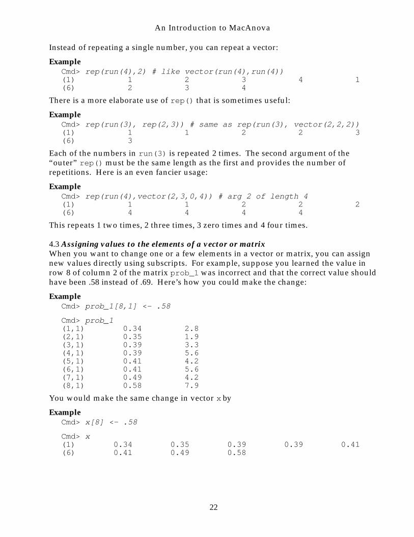
4.3 Assigning values to the elements of a vector or matrixWhen you want to change one or a few elements in a vector or matrix, you can assignnew values directly using subscripts. For example, suppose you learned the value inrow 8 of column 2 of the matrix prob_1 was incorrect and that the correct value shouldhave been .58 instead of .69. Here’s how you could make the change:
ExampleCmd> prob_1[8,1] <- .58
Cmd> prob_1(1,1) 0.34 2.8(2,1) 0.35 1.9(3,1) 0.39 3.3(4,1) 0.39 5.6(5,1) 0.41 4.2(6,1) 0.41 5.6(7,1) 0.49 4.2(8,1) 0.58 7.9
You would make the same change in vector x by
ExampleCmd> x[8] <- .58
Cmd> x(1) 0.34 0.35 0.39 0.39 0.41(6) 0.41 0.49 0.58
22

An Introduction to MacAnova
You can change several values at once:
ExampleCmd> w <- run(5)
Cmd> w(1) 1 2 3 4 5
Cmd> w[run(2)] <- vector(-10, ?)# replace 1 and 2 by -10 and MISSING
Cmd> w(1) -10 MISSING 3 4 5
Cmd> w[-run(3)] <- 17 # replace all but 1st 3 elements by 17
Cmd> w(1) -10 MISSING 3 17 17
For future use we change back prob_1[8,1] and x[8] to their original values.
Cmd> prob_1[8,1] <- .68; x[8] <- .68
4.4 Simple summaries of data in vectors and matrices – sum(), prod(), min(), max(),sort() and rank()
You use sum(), prod(), min() and max() to compute the sum of, the product of, theminimum of, and the maximum of the values in a vector.
ExampleCmd> vector(sum(y), prod(y), min(y), max(y))(1) 35.5 76723 1.9 7.9
Cmd> # check sum() and prod() by "hand" calculations
Cmd> 2.8 + 1.9 + 3.3 + 5.6 + 4.2 + 5.6 + 4.2 + 7.9(1) 35.5
Cmd> 2.8 * 1.9 * 3.3 * 5.6 * 4.2 * 5.6 * 4.2 * 7.9(1) 76723
You can use sum() to compute means, variances and standard deviations from the
basic formulas y = yi
i =1
n
∑ / n and sy
2 = yi − y ( )2
i =1
n
∑
/ n − 1( ) , and max() and min() to
compute the range ymax − ymin :Example
Cmd> n <- nrows(y); ybar <- sum(y)/n # mean
Cmd> yvar <- sum((y- ybar)^2)/(n-1) # variance
Cmd> range <- max(y) - min(y)
Cmd> vector(ybar, yvar, range) # mean, variance and range(1) 4.4375 3.6027 6
Function sort() allows you to reorder the elements in a vector in increasing order:
23

An Introduction to MacAnova
ExampleCmd> y_up <- sort(y); y_down <- sort(y,down:T)
Cmd> hconcat(y_up, y_down)(1,1) 1.9 7.9 Col. 1 is y sorted up(2,1) 2.8 5.6 Col. 2 is y sorted down(3,1) 3.3 5.6(4,1) 4.2 4.2(5,1) 4.2 4.2(6,1) 5.6 3.3(7,1) 5.6 2.8(8,1) 7.9 1.9
These also give you another way to compute the minimum and the maximum:
Cmd> vector(sort(y)[1], sort(y,down:T)[1])(1) 1.9 7.9
This last also shows that you can use subscripts directly on the values of functions.
An important way to summarize a vector of numbers is by the ranks of the elementsin the vector, with the smallest value getting rank 1, the next smallest getting rank 2,etc. You can do this in MacAnova using function rank().
ExampleCmd> a <- vector( 14.7, 13.1, 16.6, 12.9, 12.5); rank(a)(1) 4 3 5 2 1
Since 14.7 is the 4th number in order of size (there are 4–1 = 3 numbers less than 14.7) itgets rank 4, etc. When there are ties, the ranks of the tied values are the averages ofwhat would be the ranks of any tied values if they were very slightly changed so as tobreak the tie.
ExampleCmd> b <- vector( 14.7, 13.1, 16.6, 12.5, 12.5)
Cmd> rank(b)(1) 4 3 5 1.5 1.5
If the second 12.5 were modified, say to 12.500001, the two last ranks would be 1 and 2which average to 1.5.
All these functions can have matrices as arguments. In the case of sum(), prod(),min() and max(), the result is a row vector (a matrix with only one row) whichcontains the result of applying the function to each column. Both sort() and rank()compute a new matrix, the same size as the argument, with the ordered values or ranksof each column separately. Let’s apply these to prob_1:
ExampleCmd> sum(prob_1)(1,1) 3.46 35.5 Sums down columns
Cmd> prod(prob_1)(1,1) 0.0010138 76723 Products down columns
24
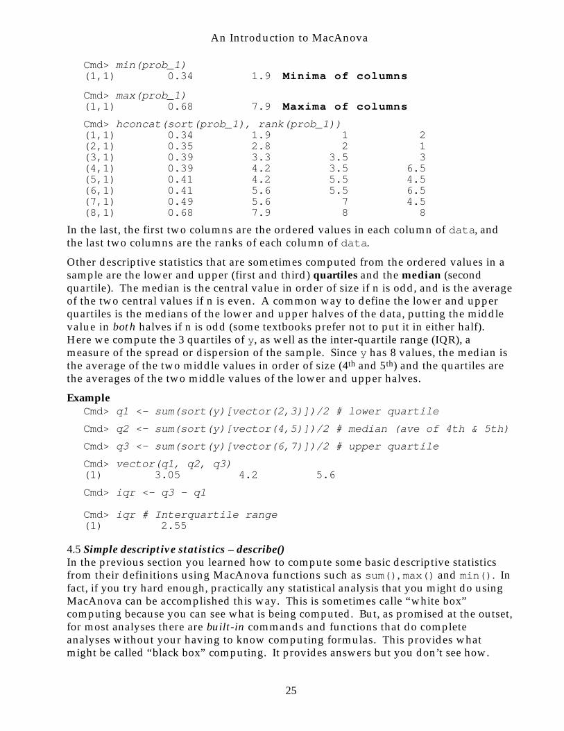
An Introduction to MacAnova
Cmd> min(prob_1)(1,1) 0.34 1.9 Minima of columns
Cmd> max(prob_1)(1,1) 0.68 7.9 Maxima of columns
Cmd> hconcat(sort(prob_1), rank(prob_1))(1,1) 0.34 1.9 1 2(2,1) 0.35 2.8 2 1(3,1) 0.39 3.3 3.5 3(4,1) 0.39 4.2 3.5 6.5(5,1) 0.41 4.2 5.5 4.5(6,1) 0.41 5.6 5.5 6.5(7,1) 0.49 5.6 7 4.5(8,1) 0.68 7.9 8 8
In the last, the first two columns are the ordered values in each column of data, andthe last two columns are the ranks of each column of data.
Other descriptive statistics that are sometimes computed from the ordered values in asample are the lower and upper (first and third) quartiles and the median (secondquartile). The median is the central value in order of size if n is odd, and is the averageof the two central values if n is even. A common way to define the lower and upperquartiles is the medians of the lower and upper halves of the data, putting the middlevalue in both halves if n is odd (some textbooks prefer not to put it in either half).Here we compute the 3 quartiles of y, as well as the inter-quartile range (IQR), ameasure of the spread or dispersion of the sample. Since y has 8 values, the median isthe average of the two middle values in order of size (4th and 5th) and the quartiles arethe averages of the two middle values of the lower and upper halves.
ExampleCmd> q1 <- sum(sort(y)[vector(2,3)])/2 # lower quartile
Cmd> q2 <- sum(sort(y)[vector(4,5)])/2 # median (ave of 4th & 5th)
Cmd> q3 <- sum(sort(y)[vector(6,7)])/2 # upper quartile
Cmd> vector(q1, q2, q3)(1) 3.05 4.2 5.6
Cmd> iqr <- q3 - q1
Cmd> iqr # Interquartile range(1) 2.55
4.5 Simple descriptive statistics – describe()In the previous section you learned how to compute some basic descriptive statisticsfrom their definitions using MacAnova functions such as sum(), max() and min(). Infact, if you try hard enough, practically any statistical analysis that you might do usingMacAnova can be accomplished this way. This is sometimes calle “white box”computing because you can see what is being computed. But, as promised at the outset,for most analyses there are built-in commands and functions that do completeanalyses without your having to know computing formulas. This provides whatmight be called “black box” computing. It provides answers but you don’t see how.
25

An Introduction to MacAnova
describe() enables you to compute in one line almost all the descriptive summarieswe have seen above. It is best introduced by an example:
ExampleCmd> describe(y) # y is the second column of prob_1component: n(1) 8 Sample sizecomponent: min(1) 1.9 Minimumcomponent: q1(1) 3.05 Lower quartilecomponent: median(1) 4.2 Median or 2nd quartilecomponent: q3(1) 5.6 Upper quartilecomponent: max(1) 7.9 Maximumcomponent: mean(1) 4.4375 Mean (average)component: var(1) 3.6027 Variance with divisor of n-1
As printed output this is pretty self-explanatory (as usual, the boldface output wasnot printed by MacAnova). It even looks as if it might have been printed bydescribe() as a “side effect.” However, what is printed is actually the value thatdescribe() returns. You can even save the value in a variable.
ExampleCmd> results <- describe(y) # nothing printed
Cmd> results$mean # extract component 'mean'(1) 4.4375 Compare with mean above
Cmd> results$var # extract component 'var'(1) 3.6027 Compare with variance above
results is an example of a new type of variable called a structure (sometimesabbreviated “STRUC”).
Cmd> list(results)results STRUC 8
Structures are made up of one or more named components. Here there are eightcomponents, n, min, q1, median, q3, max, mean and var. Individual components can beextracted by appending $cname to the name of the structure, where cname is thecomponent name. You can find all names of all the components in a structure byfunction compnames()
26

An Introduction to MacAnova
ExampleCmd> compnames(results) # the names of the components of results(1) "n"(2) "min"(3) "q1"(4) "median"(5) "q3"(6) "max"(7) "mean"(8) "var"
To make describe() compute just one summary value, say the median, you can usekeyword phrase median:T as an argument. If you want both the mean and variance,use mean:T and var:T as arguments.
ExampleCmd> describe(y,median:T) # or describe(y)$median(1) 4.2
Cmd> describe(y,mean:T,var:T) # compute both mean and variancecomponent: mean(1) 4.4375 Mean (average)component: var(1) 3.6027 Variance with divisor of n-1
You can use describe() with a matrix (table) argument, too.
ExampleCmd> describe(data1[,-1]) # summary statistics omitting column 1component: n(1) 8 8component: min(1) 0.34 1.9component: q1(1) 0.37 3.05component: median(1) 0.4 4.2component: q3(1) 0.45 5.6component: max(1) 0.68 7.9component: mean(1) 0.4325 4.4375component: var(1) 0.012079 3.6027
Each component is now a vector with one value for each column of the argumentmatrix. For example, 0.4 and 4.2 are the medians of columns 2 and 3 of data1.
describe() can also compute other statistics, the most important of which is thestandard deviation, the square root of the variance.
ExampleCmd> describe(data1[,-1],stddev:T) # square root of variance (1) 0.1099 1.8981
27

An Introduction to MacAnova
Type usage(describe) or help(describe:"?") for more information.
Several other MacAnova functions, including split(), coefs(), secoefs(),cellstats() and regpred(), compute structures as their values. Typehelp(structures:"?") or see Sec. 9.1.1 in the Users’ Guide for more informationabout structures, including functions structure() and changestr() which allow youto create or modify structures directly.
4.6 Getting help – MacAnova commands help() and usage()If you need to refresh your memory about any function or command or about generaltopics like syntax, you can use MacAnova’s help() command. Suppose you wantedmore detail on the function round() used in one of the examples above.
ExampleCmd> help(round)round(x) rounds the elements of the REAL variable x to the nearestinteger, producing a vector, matrix, or array with the same shape asx.
round(x,n) where n is an integer is equivalent to 10^(-n)*round(x*10^n). If n > 0, this rounds to n decimal places. If n < 0,this rounds to the nearest multiple of 10^abs(n). round(x,0) isequivalent to round(x).
If x is a structure, so is round(x) or round(x,n). If xi is the i-thcomponent of x, the i-th component of round(x) or round(x,n) isround(xi) or round(xi,n).
Example: round(3141.593,2) is 3141.59 and round(3141.593,-2) is 3100,the nearest multiple of 100 = 10^2.
round(x, p) can also be used when x is a CHARACTER variable and p, ifpresent, is a quoted string or CHARACTER scalar or REAL scalar. Theresult is a CHARACTER variable of the same shape as x describing thetransformation. For example, both round(vector("X1","X2"),3) andround(vector("X1","X2"),"3") return vector("round(X1,3)","round(X2,3)"). Any element of x that is "" or starts with '@', '(','[', '{', '<', '/' or '\' is not modified. This can be useful forcreating labels for a transformed variable.
See also topics floor(), ceiling(), 'structures', 'labels'.
Typically, as here, the first line gives the most standard usage, with more complexusages given later. Often, as in the last line, there are cross references to related topics.
This gives all the help on a topic. Sometimes you are looking for a specific piece ofinformation and don’t want to see everything (which can be quite long). Most helptopics have named subtopics which can be viewed individually.
28

An Introduction to MacAnova
ExampleCmd> help(round, subtopic:"?") # ask for index of subtopicsAvailable subtopics for topic 'round' are: usage structure_argument example character_argument see_alsoType help(round,subtopic:vector("subtopicA","subtopicB",...))
Cmd> help(round,subtopic:vector("usage","example"))Subtopic 'usage' of help on 'round'round(x) rounds the elements of the REAL variable x to the nearestinteger, producing a vector, matrix, or array with the same shape asx.
round(x,n) where n is an integer is equivalent to 10^(-n)*round(x*10^n). If n > 0, this rounds to n decimal places. If n <0, this rounds to the nearest multiple of 10^abs(n). round(x,0) isequivalent to round(x).
Subtopic 'example' of help on 'round'Example: round(3141.593,2) is 3141.59 and round(3141.593,-2) is 3100,the nearest multiple of 100 = 10^2.
When a topic name is no longer than 10 characters (most are), you can abbreviate this,for example, by help(round:vector("usage","example")).
Once you understand what a command or function does, command usage() may bemore useful. You use it like help() but it gives only a very brief summary of how afunction is used with no clue as to what it does.
ExampleCmd> usage(round)round(x [, ndec]), x REAL or a structure with REAL components, ndec an integer
There are hundreds of help topics. Here is how you get a list of all the topics:
ExampleCmd> help("*")Help is available on the following topics: abs evaluate macanova samplesizeacos exp macanova3 saveaddchars factor macanova_index scalarsaddhelpfile fastanova macintosh screenaddlines file_names macro secoefsadddatapath files macro_files selectaddmacrofile floor macro_syntax sethistory. . . . . . . . . . . . . . . . . . . . . . . . . . . . . . . .. . . . . . . . . . . . . . . . . . . . . . . . . . . . . . . .
29

An Introduction to MacAnova
Cmd> help() # with no arguments summarizes help() itselfType 'help(foo)' for help on topic fooType 'help(foo,subtopics:"?")' for a list of subtopics for topic fooType 'help(foo,subtopic:"bar")' subtopic bar of topic fooType 'usage(foo)' for very brief information on topic fooType 'help("*")' for a list of all topicsType 'help(help:"?")' for a list of subtopics about help().Type 'help(key:"?")' for a list of cross reference keys to topicsType 'help(usage)' for more information about usage().Some general topics are arithmetic files launching models syntax assignment glm logic notes time_series clipboard graphs macanova NULL variables comments graph_files macros number vectors complex graph_keys macro_files options workspace customize graph_ticks macro_syntax quitting data_files keywords matrices structures design labels memory subscripts data_files keywords matrices structures design labels memory subscripts
In windowed versions, selecting Help from the Help menu is equivalent to typing
help(). On a Macintosh you can press H 9 or the help key.
The topics available include all the commands and functions, plus some more generaltopics such as matrices, subscripts and transformations. To get help on a
particular topic, use help() with one or more topics as arguments.10 On theMacintosh, if you use the mouse to select a topic in the command/output window,Help from the Help menu or H or help gets help on the selected topic.
When you remember only part of the name of a topic, but not the full name, you canuse “wild card” characters “*” and “?” in a string to get a list of topics matching apattern. “*” matches any string of characters, including the empty one; “?” matchesany single topics. For example, "part*", "*part" and "*part*" match topic namesstarting with, ending with, or containing part, and "a????" matches all 5 charactertopic names starting with “a”.
ExampleCmd> help("res*") # find all topics starting with "res"resid restore resvsindex resvsrankits resvsyhatFor help on topic foo, enter help(foo) or help("foo")
Cmd> help("*plot*") # find all topics containing "plot"boxplot colplot plot showplot vboxplotchplot lineplot rowplot stringplotFor help on topic foo, enter help(foo) or help("foo")
Cmd> help("a????")anova array atanhFor help on topic foo, enter help(foo) or help("foo")
9 H means the combination of the Command key and the H key.10 In versions earlier than December 2000, you have to quote any topic names longer than 12 characters
(for example, help("transformations")), or the names of control words (while, for, break,
breakall, if, else, elseif, next).
30
An Introduction to MacAnova
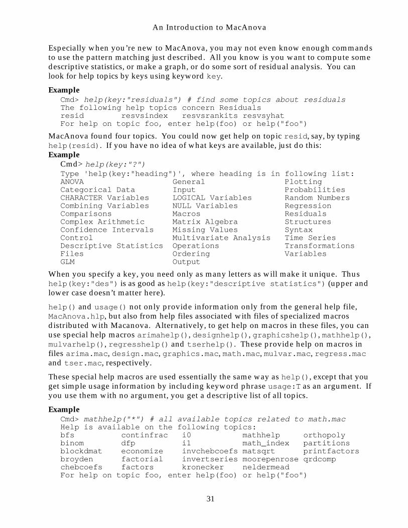
Especially when you’re new to MacAnova, you may not even know enough commandsto use the pattern matching just described. All you know is you want to compute somedescriptive statistics, or make a graph, or do some sort of residual analysis. You canlook for help topics by keys using keyword key.
ExampleCmd> help(key:"residuals") # find some topics about residualsThe following help topics concern Residualsresid resvsindex resvsrankits resvsyhatFor help on topic foo, enter help(foo) or help("foo")
MacAnova found four topics. You could now get help on topic resid, say, by typinghelp(resid). If you have no idea of what keys are available, just do this:Example
Cmd> help(key:"?")Type 'help(key:"heading")', where heading is in following list:ANOVA General PlottingCategorical Data Input ProbabilitiesCHARACTER Variables LOGICAL Variables Random NumbersCombining Variables NULL Variables RegressionComparisons Macros ResidualsComplex Arithmetic Matrix Algebra StructuresConfidence Intervals Missing Values SyntaxControl Multivariate Analysis Time SeriesDescriptive Statistics Operations TransformationsFiles Ordering VariablesGLM Output
When you specify a key, you need only as many letters as will make it unique. Thushelp(key:"des") is as good as help(key:"descriptive statistics") (upper andlower case doesn’t matter here).
help() and usage() not only provide information only from the general help file,MacAnova.hlp, but also from help files associated with files of specialized macrosdistributed with Macanova. Alternatively, to get help on macros in these files, you canuse special help macros arimahelp(), designhelp(), graphicshelp(), mathhelp(),mulvarhelp(), regresshelp() and tserhelp(). These provide help on macros infiles arima.mac, design.mac, graphics.mac, math.mac, mulvar.mac, regress.macand tser.mac, respectively.
These special help macros are used essentially the same way as help(), except that youget simple usage information by including keyword phrase usage:T as an argument. Ifyou use them with no argument, you get a descriptive list of all topics.
ExampleCmd> mathhelp("*") # all available topics related to math.macHelp is available on the following topics: bfs continfrac i0 mathhelp orthopolybinom dfp i1 math_index partitionsblockdmat economize invchebcoefs matsqrt printfactorsbroyden factorial invertseries moorepenrose qrdcompchebcoefs factors kronecker neldermeadFor help on topic foo, enter help(foo) or help("foo")
31
An Introduction to MacAnova
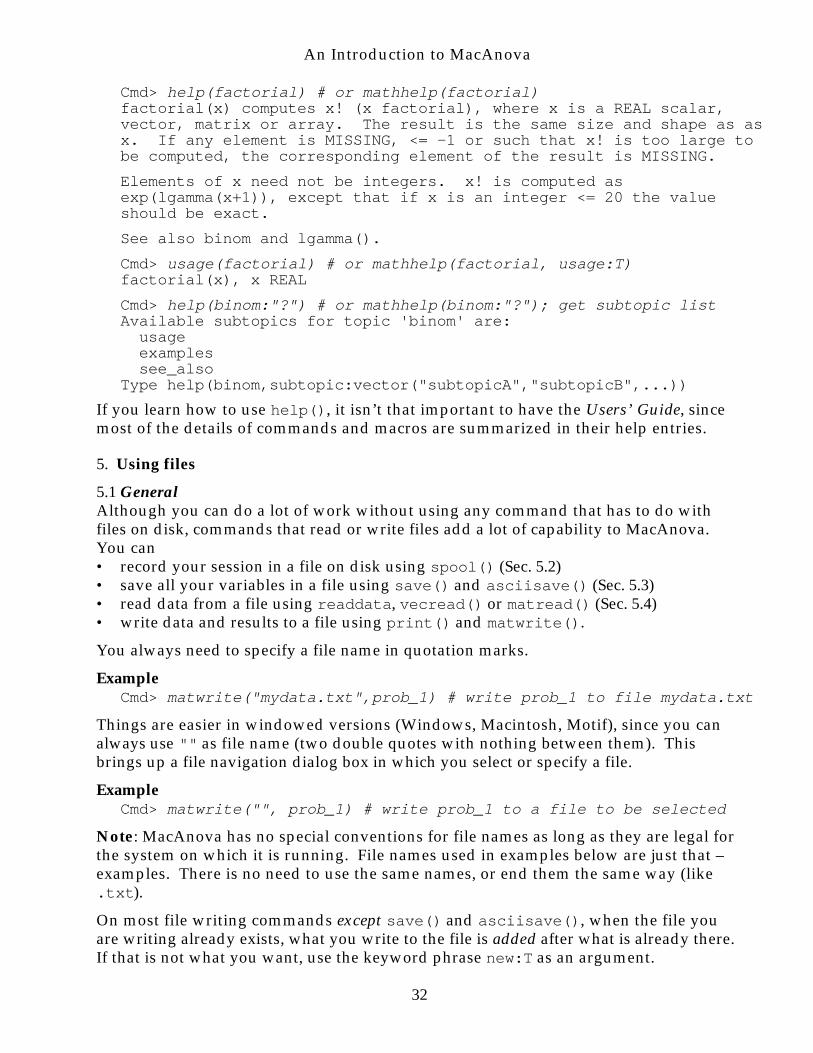
Cmd> help(factorial) # or mathhelp(factorial)factorial(x) computes x! (x factorial), where x is a REAL scalar,vector, matrix or array. The result is the same size and shape as asx. If any element is MISSING, <= -1 or such that x! is too large tobe computed, the corresponding element of the result is MISSING.
Elements of x need not be integers. x! is computed asexp(lgamma(x+1)), except that if x is an integer <= 20 the valueshould be exact.
See also binom and lgamma().
Cmd> usage(factorial) # or mathhelp(factorial, usage:T)factorial(x), x REAL
Cmd> help(binom:"?") # or mathhelp(binom:"?"); get subtopic listAvailable subtopics for topic 'binom' are: usage examples see_alsoType help(binom,subtopic:vector("subtopicA","subtopicB",...))
If you learn how to use help(), it isn’t that important to have the Users’ Guide, sincemost of the details of commands and macros are summarized in their help entries.
5. Using files
5.1 GeneralAlthough you can do a lot of work without using any command that has to do withfiles on disk, commands that read or write files add a lot of capability to MacAnova.You can• record your session in a file on disk using spool() (Sec. 5.2)• save all your variables in a file using save() and asciisave() (Sec. 5.3)• read data from a file using readdata, vecread() or matread() (Sec. 5.4)• write data and results to a file using print() and matwrite().
You always need to specify a file name in quotation marks.
ExampleCmd> matwrite("mydata.txt",prob_1) # write prob_1 to file mydata.txt
Things are easier in windowed versions (Windows, Macintosh, Motif), since you canalways use "" as file name (two double quotes with nothing between them). Thisbrings up a file navigation dialog box in which you select or specify a file.
ExampleCmd> matwrite("", prob_1) # write prob_1 to a file to be selected
Note: MacAnova has no special conventions for file names as long as they are legal forthe system on which it is running. File names used in examples below are just that –examples. There is no need to use the same names, or end them the same way (like.txt).
On most file writing commands except save() and asciisave(), when the file youare writing already exists, what you write to the file is added after what is already there.If that is not what you want, use the keyword phrase new:T as an argument.
32

An Introduction to MacAnova
ExampleCmd> matwrite("mydata",prob_1,new:T) # prob_1 to end of mydata.txt
In the windowed versions, when you save the command/output window using SaveWindow or Save Window As on the File menu, it is always as if you specified new:T.
5.2 Recording your MacAnova session – spool()When you use MacAnova you may want a record of what you do, or at least a perma-nent copy of the answers you want to keep. This is quite easy to do using spool() – aslong as you remember to use it! spool() works on all computer systems, Windows,DOS, Macintosh, Motif or Linux/Unix.
spool() keeps a record in a file of some or all of your MacAnova session. When youwant to start saving stuff, you need to type something like
Cmd> spool("spool.txt") # start spooling on file spool.txt
This starts recording (spooling) on file spool.txt. From now on, everything you typeand everything MacAnova replies except high resolution plots will be written in thefile. Of course, this includes any mistakes you make and your false starts. In thewindowed versions, you don’t need to type the file name but can type
Cmd> spool("") # Null file name allowed only in windowed versions
If you want to suspend spooling for a while, simply type
Cmd> spool() # with no file nameSpooling on spool.txt suspended
When you want to start recording again, type
Cmd> spool() # again with no file nameResume spooling on spool.txt
Once you have started spooling, spool(), with no argument, toggles it off and on.
On a Macintosh, selecting entry Spool Output to File on the File menu is equivalentto typing spool("") or spool().
When you are done with your session, you can read the spool file into almost any wordprocessor or text editor, edit out what you don’t want to keep and add your commen-tary.
Here’s a useful tip: If your word processor or editor lets you choose a font, select a fontsuch as Courier or Monaco that has equal width characters. If you don’t, things thatlined up on the computer screen will not line up in your document and will be hard toread.
You don’t need spool() as much in a windowed version since all your input andMacAnova’s output remain in the command/output window. At any time you can
select Save Window ( S or Ctrl+S 11) or Save Window As… on the File menu andthe entire contents of the window are written to disk for later editing. After a windowis saved, the name of the file becomes the window title and you can re-save the
11 Ctrl+S means the combination of the Control key and the S key.
33
An Introduction to MacAnova
window just by pressing S (Macintosh) or Ctrl+S (Windows and Motif). It’s a goodidea to do this frequently so as to avoid losing much work in case of a computer crash.
When you quit in windowed versions, a dialog box asks Save Changes to Window"xxxxx" before closing? To save the command/output window on disk, just clickon the OK button (or the Don’t Save button if you don’t want to).
Important: Saving the window does not save your workspace – your data and othervariables and macros. For that you need commands save() or asciisave() (Sec. 5.3).
You can also use commands print(file:"fileName",...) andwrite(file:"fileName",...) to print the values of individual variables in a file.See the Users’ Guide or type help(print,write).
5.3 Saving your workspace – save() and asciisave()Sometimes you may not have time to do everything you want or need to in onesession, and still have more to do when you have to quit. In such a situation you canuse save() and asciisave(). These functions save your “workspace” in a file in aform that can be restored by restore() in a later MacAnova session. Your workspaceconsists of all the current variables, macros and graphs in graph windows.
Important: save() and asciisave() do not save your commands and output. Usespool() or Save Window on the File menu for that (Sec. 5.2).
ExampleCmd> save("savework.sav")Workspace saved on file savework.sav
You can now quit MacAnova. Later, when you restart, you can use restore() to geteverything back to the way it was.
ExampleCmd> restore("savework.sav") # restore("") in windowed versionsRestoring workspace from file savework.savWorkspace saved Sun Jul 8 23:35:33 2001
In windowed versions, you can use Save Workspace ( K or Ctrl+K) or SaveWorkspace As… on the File menu, instead of save().
On a Macintosh, the next time you want to start up MacAnova, just double click on the
icon of the saved file and MacAnova will be launched with everything restored,
including any graph windows. At the same time you save your workspace in thewindowed versions, you may also want to save the command/output window usingitems Save Window ( S or Ctrl+S) or Save Window As… on the File menu.
If you use MacAnova on more than one type of computer, you might occasionally starton one computer, say a Macintosh, save your work, and then finish it later on anothertype, say a Windows computer. For this you should save your workspace usingasciisave() instead of save().
34

An Introduction to MacAnova
ExampleCmd> asciisave("savework.asc")Workspace saved on file savework.asc
This produces an ordinary text file which can be restored by MacAnova on anycomputer (by restore("savefile.asc")) or even sent via E-mail.
save() can also be a life saver if your computer is unstable and prone to crashing, or if,perish the thought, your copy of MacAnova has a bug that sometimes causes a crash. Ifyou save your workspace and your window from time to time, you never will losemuch if the computer or program goes down.
After you have used save("savework.sav") or asciisave("savework.sav") once,you can update the save file simply by save() or asciisave(), without specifying afile name. In windowed versions, select Save Workspace ( K or Ctrl+K) on the Filemenu.
Once you have saved your window, you can refresh the file by selecting Save Window( S or Ctrl+S) on the File menu.
5.4 Reading data from files – vecread() , readdata() and matread()Except when you analyze a small amount of data that you can easily type at thekeyboard, you will probably want to work with data that is in a file on disk. The datamay have been provided by someone else, entered by you using a word processor oreditor or possibly exported from a spreadsheet.
Any data file MacAnova can read must be a plain text file. It might be created in aword processor such as Microsoft Word or a text editor such as SimpleText (Macintosh)or Note Pad (Windows). If you use a word processor to create or edit data files, it isessential that they be saved as Text or ASCII files. How you do it depends on theprogram. If a file is not saved as a Text or ASCII file, MacAnova will not be able to readit.
The simplest type of data file MacAnova can read contains just numbers. Here is alisting of file rabbit.txt containing 12 determinations of the survival time inminutes of certain rabbit nerves under anaerobic conditions:
16.2 22.5 21.4 19.6 24.8 21.4 19.0 14.7 13.3 23.0 16.8 20.1
Before going further, you might want to use an editor or word processor to create thisfile and other example files in this section. Be sure to save them as a plain text(sometimes called ASCII) files. Copies of the example files are available on the web.
Here’s one way to read these data from the file:
ExampleCmd> x <- vecread("rabbit.txt")# form is vecread(fileName)Read from file "KB1:MacAnova:Datafiles:rabbit.txt"
Cmd> x # print out what you've read in (1) 16.2 22.5 21.4 19.6 24.8 (6) 21.4 19 14.7 13.3 23(11) 16.8 20.1
35
An Introduction to MacAnova
vecread() reads the numbers in the file sequentially, line by line to the end, andreturns them as a vector.
• A question mark (?) in the file is interpreted as MISSING. Also an isolated “.” , “*”or “NA” is interpreted as MISSING.
• Any lines starting with “#” are skipped.
• If there is a “!” at any point in the file except in a line starting with “#”, vecread()stops reading there.
Suppose rabbit1.txt looks like this:
# Survival time in minutes of rabbit nerves 16.2 22.5 21.4 19.6 24.8 21.4 19.0 14.7 13.3 23.0 16.8 20.1
ExampleCmd> x <- vecread("rabbit1.txt")Read from file "KB1:Datafiles:rabbit1.txt"
Cmd> x # same as before (1) 16.2 22.5 21.4 19.6 24.8 (6) 21.4 19 14.7 13.3 23(11) 16.8 20.1
When vecread() finds anything it can’t read, it skips it, printing a warning messagethe first time something unreadable is hit.
Suppose file rabbit2.txt looks like this, with a line without numbers:
Data on twelve rabbit nerves 16.2 22.5 21.4 19.6 24.8 21.4 19.0 14.7 13.3 23.0 16.8 20.1
ExampleCmd> x <- vecread("rabbit2.txt"); xWARNING: nonnumeric character(s) in KB1:Datafiles:rabbit2.txt ignoredRead from file "KB1:Datafiles:rabbit2.txt"
Cmd> x # data are correct (1) 16.2 22.5 21.4 19.6 24.8 (6) 21.4 19 14.7 13.3 23(11) 16.8 20.1
But when another file rabbit3.txt looks like this
Data on 12 rabbit nerves 16.2 22.5 21.4 19.6 24.8 21.4 19.0 14.7 13.3 23.0 16.8 20.1
you will be in trouble because the 12 is read as a number and vecread() would return13 numbers, the value 12 followed by the actual data.
36

An Introduction to MacAnova
ExampleCmd> x <- vecread("rabbit3.txt"); xWARNING: nonnumeric character(s) in KB1:Datafiles:rabbit3.txt ignoredRead from file "KB1:Datafiles:rabbit3.txt" (1) 12 16.2 22.5 21.4 19.6 (6) 24.8 21.4 19 14.7 13.3(11) 23 16.8 20.1
So, to be on the safe side, a file to be read by vecread() should contain only numbersexcept in lines starting with “#”.
Many data files have several columns of numbers or symbols, with each columncorresponding to a variable and each line to the data for a case. A typical examplemight be file crops.txt:
# yields of wheat and potatoes by year 1926 20.1 7.2 1927 23.6 7.1 1928 26.3 7.4 1929 19.9 6.1 1930 16.7 6.0 1931 23.2 7.3 1932 31.4 9.4 1933 33.5 9.2 1934 28.2 8.8 1935 35.3 10.4 1936 29.3 8.0 1937 30.5 9.7
The number in column 1 is a year and columns 2 and 3 are the average yields of wheatand potatoes, respectively, in each year. You can use readdata() to read crops.datinto three MacAnova variables, year, wheat and potatoes:
ExampleCmd> readdata("crops.txt",year,wheat,potatoes)# yields of wheat and potatoes by yearRead from file "KB1:Datafiles:crops.txt"year saved as REAL vectorwheat saved as REAL vectorpotatoes saved as REAL vector
Cmd> print(year,wheat,potatoes)year: (1) 1926 1927 1928 1929 1930 (6) 1931 1932 1933 1934 1935(11) 1936 1937wheat: (1) 20.1 23.6 26.3 19.9 16.7 (6) 23.2 31.4 33.5 28.2 35.3(11) 29.3 30.5potatoes: (1) 7.2 7.1 7.4 6.1 6 (6) 7.3 9.4 9.2 8.8 10.4(11) 8 9.7
readdata() uses vecread() to read the file. Consequently it recognizes “?”, “.”, “*”
37

An Introduction to MacAnova
and “NA” as MISSING, skips lines that start with “#” and stops reading when it finds“!”.
readdata() can also read categorical data and can take the names of the variablesfrom a file. Suppose mont5-1.txt looks like this:
# example 5-1 on page 129 of Montgomery.specimen tiptype depth 1 A 9.3 2 A 9.4 3 A 9.6 4 A 10.0 1 B 9.4 2 B 9.3 3 B 9.8 4 B 9.9 1 C 9.2 2 C 9.4 3 C 9.5 4 C 9.7 1 D 9.7 2 D 9.6 3 D 10.0 4 D 10.2
ExampleCmd> readdata("mont5-1.txt") # Note: no variable names are supplied# example 5-1 on page 129 of Montgomery.Read from file "KB1:Datafiles:mont5-1.txt"specimen saved as REAL vectortiptype saved as factordepth saved as REAL vector
Cmd> print(specimen,tiptype,depth)specimen: (1) 1 2 3 4 1 (6) 2 3 4 1 2(11) 3 4 1 2 3(16) 4tiptype: A A A A B B B B C C C C D D D D 1 1 1 1 2 2 2 2 3 3 3 3 4 4 4 4depth: (1) 9.3 9.4 9.6 10 9.4 (6) 9.3 9.8 9.9 9.2 9.4(11) 9.5 9.7 9.7 9.6 10(16) 10.2
tiptype looks a little different. The actual values are the numbers; the originalcharacter factor codes (A, B, C and D) have been preserved as case labels. MacAnova
38

An Introduction to MacAnova
prints all the labels of a vector before any of the values.
ExampleCmd> describe(tiptype,min:T,max:T)component: min(1) 1component: max(1) 4
matread() is designed to read data sets from files containing many data sets. This issomething neither vecread() or readdata can easily do. However, each data set mustbe in a special format. See the Users’ Guide or type help(matread_file) for detailson the actual format matread() expects.
All you need to know here is that the first line of every data set contains its name anddimensions and may be followed by descriptive comments. To read in a particular dataset you specify the name of the file and the name of the data set. In the followingexample, file crops1.txt contains several data sets including a data set named yieldswhich contains the same data as crops.txt.
ExampleCmd> data <- matread("crops1.txt","yields")yields 12 3) Col. 1: year) Col. 2: wheat = wheat harvest) Col. 3: potatoes = potato harvestRead from file "KB1:Datafiles:crops1.txt"
Cmd> dim(data) # data is a matrix with 12 rows and 3 columns(1) 12 3
Cmd> yields[vector(1,2),] # cases 1 and 2(1,1) 1926 20.1 7.2(2,1) 1927 23.6 7.1
The first line printed, “yields 12 3”, is the line in the file with the data setname and dimensions . The remaining lines, all starting with “)”, are descriptivecomments in the file. “)” serves a similar purpose in files to be read by matread() as“#” does in files read by readdata() and vecread().
To get each column in a separate variable, you can either do it “by hand” or usemakecols():
ExampleCmd> year <- data[,1]; wheat <- data[,2]; potatoes <- data[,3]
Cmd> list(year,wheat,potatoes)# you have three 12 by 1 matricespotatoes REAL 12 1 wheat REAL 12 1 year REAL 12 1
Cmd> makecols(data,year,wheat,potatoes)
Cmd> list(year,wheat,potatoes)# now you have three length 12 vectorspotatoes REAL 12 wheat REAL 12 year REAL 12
39

An Introduction to MacAnova
5.5 Moving data from and to a spreadsheetThere are lots of reasons why you might have data in a spreadsheet and want to analyzeit in MacAnova. For one thing, it’s probably easier to enter lots of data into a spread-sheet than directly in MacAnova using vector(). Conversely, you may want to saveresults from a MacAnova analysis in a spreadsheet. Moving numbers either way iseasy to do using the Clipboard in the windowed versions of MacAnova.
The Clipboard is a place for temporarily saving information in one program so it can berecovered in another program.
Suppose you have the data from file mont5-1 in an Excel spreadsheet, and you want totransfer the depth data to MacAnova. All you need to do is to use the mouse to selectthe data to transfer and then select Copy on the Edit menu to put it on the Clipboard..
Then switch over to MacAnova and use fromclip to create a numerical vector fromwhat you copied to the Clipboard.
Cmd> depth <- fromclip()
Cmd> depth (1) 9.3 9.4 9.6 10 9.4 (6) 9.3 9.8 9.9 9.2 9.4(11) 9.5 9.7 9.7 9.6 10(16) 10.2
clipreaddata() would also do the job. It works similarly to readdata() except it“reads” the Clipboard instead of a file.
Cmd> clipreaddata(depth)depth saved as REAL vector
40
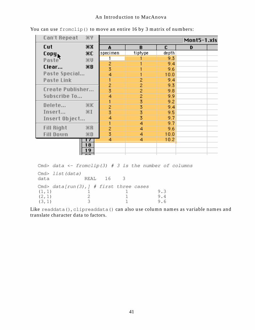
An Introduction to MacAnova
You can use fromclip() to move an entire 16 by 3 matrix of numbers:
Cmd> data <- fromclip(3) # 3 is the number of columns
Cmd> list(data)data REAL 16 3
Cmd> data[run(3),] # first three cases(1,1) 1 1 9.3(2,1) 2 1 9.4(3,1) 3 1 9.6
Like readdata(), clipreaddata() can also use column names as variable names andtranslate character data to factors.
41

An Introduction to MacAnova
Example
Cmd> clipreaddata() # reads data on clipboard to variablesspecimen saved as REAL vectortiptype saved as factordepth saved as REAL vector
Cmd> list(specimen,tiptype,depth)depth REAL 16 specimen REAL 16 tiptype REAL 16 FACTOR with 4 levels
Note that the area selected in the spreadsheet includes the column headings.
Important: If any of the data in the spreadsheet is missing, you must use one of theMacAnova codes, “?”, “.”, “*” or “NA”, for MISSING. It won’t work just to leave thespreadsheet cell empty.
To go in the other direction, from MacAnova to the spreadsheet is just as simple.Here’s how you would export matrix prob_1 to a spreadsheet.
Cmd> list(prob_1) # you need the dimensionsprob_1 REAL 8 2
Cmd> toclip(prob_1) # puts the matrix on the Clipboard
42

An Introduction to MacAnova
Now you need to switch the spreadsheet program, use the mouse to select a rectangle of16 cells in 8 rows and 2 columns and then choose Paste from the Edit menu:
43
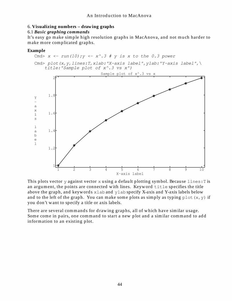
An Introduction to MacAnova
6. Visualizing numbers – drawing graphs6.1 Basic graphing commandsIt’s easy go make simple high resolution graphs in MacAnova, and not much harder tomake more complicated graphs.
ExampleCmd> x <- run(10);y <- x^.3 # y is x to the 0.3 power
Cmd> plot(x,y,lines:T,xlab:"X-axis label",ylab:"Y-axis label",\title:"Sample plot of x^.3 vs x")
1
1.2
1.4
1.6
1.8
2
1 2 3 4 5 6 7 8 9 10
Sample plot of x^.3 vs x
X-axis label
Y-axis label
This plots vector y against vector x using a default plotting symbol. Because lines:T isan argument, the points are connected with lines. Keyword title specifies the titleabove the graph, and keywords xlab and ylab specify X-axis and Y-axis labels belowand to the left of the graph. You can make some plots as simply as typing plot(x,y) ifyou don’t want to specify a title or axis labels.
There are several commands for drawing graphs, all of which have similar usage.Some come in pairs, one command to start a new plot and a similar command to addinformation to an existing plot.
44

An Introduction to MacAnova
Command Description
plot(x,y) Plot each column of vector or matrix y againstvector x using standard symbols
addpoints(x,y) Add points to a previously plotted graph usingstandard symbols
chplot(x,y,symbols:symb) Like plot() except you can specify plotting symbolsspecified by symb
addchars(x,y,symbols:symb) Add points to a previously plotted graph usingcustom symbols
lineplot(x,y) Like plot() without plotting symbols but withconnecting lines
addlines(x,y) Add lines to a previously plotted graph
stringplot(x,y,strings:s) Like plot() but drawing character strings specifiedby s
addstrings(x,y,strings:s) Add character strings to previously plotted graph
showplot() Redisplay the most recent plot, possibly with newlabels and changed minima or maxima.
vboxplot(x), vboxplot(str)boxplot(x), boxplot(str)
Make parallel vertical or horizontal boxplots of datain columns of matrix x or components of structurestr
For the x-y plotting commands (plot() through addstrings()), x must be a REALvector and y must be a REAL vector or matrix (only a vector for stringplot() andaddstrings()). The values in each column of y are plotted against the values in x.
Ordinarily, x and y must have the same number of rows. For chplot() andaddchars(), symb is a CHARACTER vector or a vector of integers between 0 and 999. Forstringplot() and addstrings(), s is a CHARACTER scalar or vector.
For stringplot() and addstrings(), x and y must be vectors of the same length.For the other x-y plotting commands, x can be a scalar or vector of length 2, regardlessof the length of y.
• When x is just one number x0, it is implicitly expanded to vector(x0, x0+1,...)with the same number of rows as y. For example, plot(1,y) plots y against 1, 2, 3,... and plot(100,y) plots y against 100, 101, 102, ... .
• When x is vector(x0,inc) of length 2, it is implicitly expanded to vector(x0,x0+inc, x0+2*inc,...) with the same number of rows as y. For example,plot(vector(0,1/60),y) plots y against 0, 1/60, 2/60, .... andlineplot(vector(1967, 1/12),y) plots y against 1967, 1967+1/12, 1967+2/12, ... .You might use this last when the rows of y are monthly values starting January1967 and you want to plot y against time in years.
Help topic graphs includes a lot of information about graphing. Start out by typinghelp(graphs:"?") to get a list of subtopics and then help(graphs:"name"), where
45
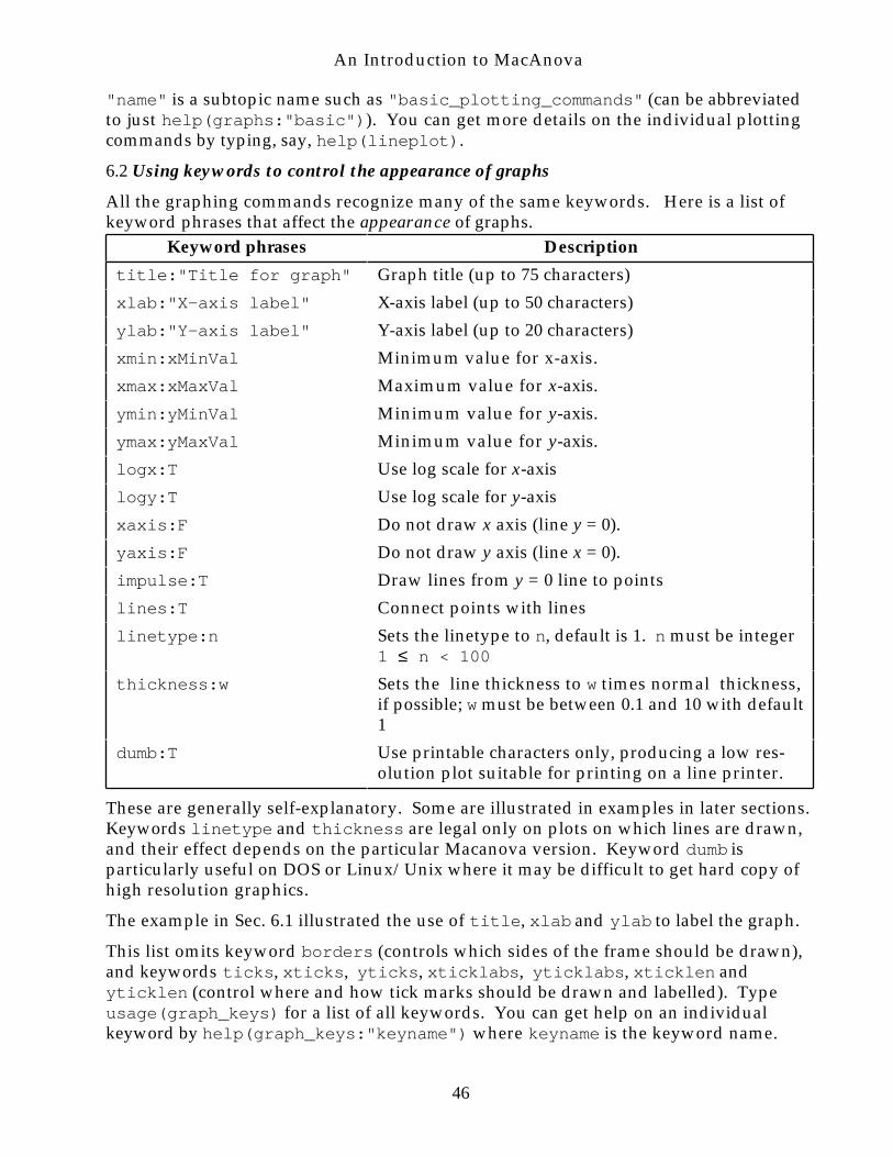
An Introduction to MacAnova
"name" is a subtopic name such as "basic_plotting_commands" (can be abbreviatedto just help(graphs:"basic")). You can get more details on the individual plottingcommands by typing, say, help(lineplot).
6.2 Using keywords to control the appearance of graphs
All the graphing commands recognize many of the same keywords. Here is a list ofkeyword phrases that affect the appearance of graphs.
Keyword phrases Description
title:"Title for graph" Graph title (up to 75 characters)
xlab:"X-axis label" X-axis label (up to 50 characters)
ylab:"Y-axis label" Y-axis label (up to 20 characters)
xmin:xMinVal Minimum value for x-axis.
xmax:xMaxVal Maximum value for x-axis.
ymin:yMinVal Minimum value for y-axis.
ymax:yMaxVal Minimum value for y-axis.
logx:T Use log scale for x-axis
logy:T Use log scale for y-axis
xaxis:F Do not draw x axis (line y = 0).
yaxis:F Do not draw y axis (line x = 0).
impulse:T Draw lines from y = 0 line to points
lines:T Connect points with lines
linetype:n Sets the linetype to n, default is 1. n must be integer1 ≤ n < 100
thickness:w Sets the line thickness to w times normal thickness,if possible; w must be between 0.1 and 10 with default1
dumb:T Use printable characters only, producing a low res-olution plot suitable for printing on a line printer.
These are generally self-explanatory. Some are illustrated in examples in later sections.Keywords linetype and thickness are legal only on plots on which lines are drawn,and their effect depends on the particular Macanova version. Keyword dumb isparticularly useful on DOS or Linux/Unix where it may be difficult to get hard copy ofhigh resolution graphics.
The example in Sec. 6.1 illustrated the use of title, xlab and ylab to label the graph.
This list omits keyword borders (controls which sides of the frame should be drawn),and keywords ticks, xticks, yticks, xticklabs, yticklabs, xticklen andyticklen (control where and how tick marks should be drawn and labelled). Typeusage(graph_keys) for a list of all keywords. You can get help on an individualkeyword by help(graph_keys:"keyname") where keyname is the keyword name.
46

An Introduction to MacAnova
ExampleCmd> help(graph_keys:"borders")Subtopic 'borders' of help on 'graph_keys' borders:Word Controls which sides of the graph borders will be drawn. Word can be "all", "none", "", or a combination of one or more of "B", "b", "L", "l", "T", "t", "R", "r". See topic 'graph_border'.
6.3 GRAPH variables and modifying graphsNormally, whenever MacAnova draws a graph, it also creates variable LASTPLOTwhich encapsulates all the information used to create the plot. LASTPLOT has thespecial type GRAPH.
You can’t calculate with a GRAPH variable, but you can assign it to another variable (forexample, plot1 <- LASTPLOT) and you can print it to produce a low resolution plotsimilar to that produced by the plotting commands when dumb:T is used.
More importantly, you can redisplay the graph encapsulated in a GRAPH variable,possibly with changed labeling information and/or additional data.
Cmd> showplot()
redisplays the graph in LASTPLOT, that is, the most recent graph.
Cmd> showplot(xlab:"x", ylab:"Power of x", ymin:0)
displays it with new x- and y-axis labels, and with 0 as the y-axis minimum. It alsomodifies LASTPLOT to include the new information. You can use all the keywordphrases listed above except lines, impulse, linetype and thickness to change oradd labelling information or to set the minimum or maximum values to appear in thegraph.
Cmd> addpoints(x1, y1)
redisplays LASTPLOT, adding additional points from the data in x1 and y1. You cansimilarly use addlines(), addchars(), and addstrings() to display the graphencapsulated in LASTPLOT with additional data included in the plot.
Cmd> plot1 <- LASTPLOT # duplicate of GRAPH variable LASTPLOT
Cmd> showplot(plot1,title:"Redisplayed with a new title”)
This displays the graph encapsulated in plot1. You can use the usual keywords. Itdoesn’t change plot1, but updates LASTPLOT to reflect the new graph.
Cmd> addpoints(plot1, x2, y2) # redisplays plot1 with more data
47

An Introduction to MacAnova
Here is an example in which we redo the plot in Sec. 6.1 and add more line-connectedpoints using several keywords, interpreted as follows:
symbols:"\1" Plot the data using a special plotting symbol; symbol "\1" isdiamond; "\6" is the default symbol; "\7" is a dot
lines:T Connect the points with lines
ymin:0 Minimum for y axis is 0
ymax:y[10]^2 Maximum for y axis is y[10]^2
title:" ... " Provides a new title replacing the original one
ExampleCmd> plot(x,y,lines:T,xlab:"X-axis label",ylab:"Y-axis label",\
title:"Sample plot of x^.3 vs x", show:F) # see below for show:F
Cmd> addchars(x,y^2,symbols:"\1",lines:T,\title:"Plot redrawn using addchars", ymin:0,ymax:y[10]^2)
0
0.5
1
1.5
2
2.5
3
3.5
4
1 2 3 4 5 6 7 8 9 10
Plot redrawn using addchars
X-axis label
Y-axis label
48

An Introduction to MacAnova
Cmd> showplot(dumb:T,title:"Plot redrawn using dumb:T",\height:23,width:70)
Plot redrawn using dumb:T ++-----+-----+-----+-----+-----+-----+-----+-----+------++ 4+ .o+ | .... | | ...o. | 3.5+ ...o.. + Y | ...o.. | - 3+ ...o.. + a | .o.. | x 2.5+ ... + i | ...o. | s 2+ .o.. ...*......*+ | ... ...*.....*.....*.. | l 1.5+ .o. ...*.....*.. + a | ....*.....*.. | b 1+o.. + e | | l 0.5+ + | | 0+........................................................+ ++-----+-----+-----+-----+-----+-----+-----+-----+------++ 1 2 3 4 5 6 7 8 9 10 X-axis label
The second plot illustrates how to use showplot() with argument dumb:T to make alow resolution plot using ordinary typographical symbols. height:23 and width:70specify the number of rows (lines) and columns (characters per line). The defaultvalues are 24 and 80. The smaller values were used so it would fit on this page.
A “dumb” plot like this is not as elegant as a high resolution graph, but can be printedon any printer, and included in any word processor document. If you are usingspool() to save your input and output, any “dumb” plots are written to the spoolingfile, but high resolution plots are not.
Here are two additional keywords related to modifying or redisplaying graphs:
Keyword phrases Description
keep:F Do not save plot as LASTPLOT.
show:F Do not display plot, only save.
When a graph is complicated, LASTPLOT can use a lot of room in your workspace. Ifyou don’t plan to modify the plot you can save memory by including keep:F as anargument on any graphics command.
When you are building a complicated graph in stages by adding different types ofinformation, you may not want to see the graph until it is finished. If so, use show:Fon every plotting command except the last one. This was illustrated in producing theplot on the preceding page.
It is an error to use both show:F and keep:F.
49

An Introduction to MacAnova
6.4 Graphs in a windowed versionIn the windowed versions (Windows, Macintosh, Motif), there are eight basic graphwindows, Graph 1, Graph 2, ..., Graph 8. A new plot normally goes in the lowestnumbered available window, but keyword phrase window:n, where n is an integerbetween 0 and 8 puts it in window n (window:0 puts it in the most recently usedwindow). When the window is in front, you can print it by selecting Print Graph onthe File menu. You can copy the graph to the Clipboard using Copy on the Edit menu(not Motif).
On a Macintosh, but not the other versions, there are two additional windows, Panelof Graphs 1-4 and Panel of Graphs 5-8 which display the contents of the regulargraph windows in reduced size. Copy on the Edit menu and Print Graph on the Filework with these, too. When a Panel of Graphs window is in front, clicking on any ofthe panels brings the corresponding graph window to the front.
You can switch to any graph window by clicking in it, selecting it on the Windowsmenu or by pressing an appropriate combination of keys.
On a Macintosh, you switch to a graph window by pressing one of 1, 2, ..., 8, orF1, ..., or F8. Pressing G displays a Panel of Graphs window or toggles between
such windows.
In Windows, you press Ctrl+F1, Ctrl+F2, ..., or Ctrl+F8 to switch to a graph window.
In Motif, you press Ctrl+1, Ctrl+2, ..., or Ctrl+8 to switch to a graph window.
When a graph window is in front, hitting Return or Enter brings the command/outputwindow forward.
The size of a dumb graph is determined by the size of the command/output window,but can be modified by keywords height and width, as illustrated in the example inSec. 6.3.
6.5 Plotting under DOSWhen running under DOS, there is only one window. A high resolution plot replacesits contents. Hitting Return, erases the graph and returns to command mode, refreshingany commands and output that were on the screen before the plot.
DOS has no automatic facilities for doing anything with a graph. However, whenrunning a DOS version under Windows 95/98/NT you can copy the graph to theclipboard by pressing ALT-PrintScreen.
6.6 Plotting under Linux/UnixMacAnova on Linux or Unix (non-Motif) assumes that you are using a terminal thatcan emulate a Tektronix 4014 terminal, a once popular graphical device. MacAnovatranslates the information to be plotted, including plot frames, boundary ticks, labels,lines and points into the arcane sequences of characters that a Tektronix 4014 terminalexpects.
In particular, the popular xterm pseudo VT100 window on many workstations canemulate a Tektronix 4014, but not some more modern replacements like dtterm and
50

An Introduction to MacAnova
hpterm. If MacAnova is running in a xterm window, a Tektronix graphics window isopened and drawn to. After a Return is hit, it then switches back to the VT100 window.If you get just a sequence of funny characters when you try to make a high resolutionplot in Linux or Unix, it probably means Tektronix emulation is not enabled.
Since few users now use Tektronix 4014 emulators, no further details are given here.Type help(tek,vt,options:"tekset") for some further information.
6.7 Incorporating a graph in word processor documentThe only universally applicable way to do this is to write a “dumb” plot to a file andthen open the file in the word processor.
If you have started spooling your output using spool(), “dumb” plots are automat-ically included in the spooled output. Alternatively, you can use showplot() to writea GRAPH variable to a file as a low resolution plot. Thus
ExampleCmd> showplot(file:"myplots.txt",dumb:T)
writes the plot encapsulated in LASTPLOT to file myplots.txt as a “dumb” plot. SeeSec. 6.8 for other ways to write graphs to a file.
On a Macintosh or in Windows you can copy high resolution graphs to the Clipboard.When a graphics window is the front window, select Copy on the Edit menu ( C orCtrl+C). Then switch to a word processor document or a graphics editor window andselect Paste on the Edit menu ( V or Ctrl+V).
In the DOS versions, under Windows 95/98/NT you can copy a high resolution graphto the Clipboard by pressing ALT-PrintScreen while the MacAnova plot is on the screen.Under DOS without Windows, no such direct copying of the graphics screen is possible.
6.8 Writing graphs to filesBesides a dumb plot, there are other forms in which you can write a graph to a file. Themost important way is as PostScript commands. PostScript is a powerful pagedescription language recognized by certain printers, including Apple LaserWriters. Itcan represent any graph that MacAnova can produce.
Other forms are as a PICT file (Macintosh only), a PCX file (extended memory DOSversion only) or as a sequence of Tektronix 4014 commands (Linux and Unix only).
51

An Introduction to MacAnova
Here are keywords phrases associated with writing graphs to files:
Keyword phrases Description
file:fileName Write PostScript to file fileName without displaying theplot.
file:fileName,dumb:T Write a low resolution plot to file fileName withoutdisplaying the plot.
new:T Clear file fileName before writing
landscape:T(used only with file)
PostScript plot will be rotated so as to fill a 8.5" by 11" page.
ps:F(used only with file)
Suppresses PostScript when writing a plot to a file. On aMacintosh a PICT file is written; on Linux and Unix,Tektronix 4014 plotting commands are written to the file; onother computers, a “dumb” plot is written to the file.
screendump:fileName On a Macintosh a PICT file is written; on extended memoryDOS version a PCX file is written; illegal in other versions.
epsf:T On a Macintosh, when used with file:fileName, anencapsulated PostScript file is written
ExampleCmd> showplot(file:"myplots.ps",new:T)
This writes a PostScript description of the graph encapsulated in LASTPLOT to filemyplots.ps. On the first use of file:"myplots.ps", you should include new:T as anargument. Subsequent writes should omit new:T or have new:F.
It is beyond the scope of this document to explain what to do with the PostScript filewhen you leave MacAnova. On some Linux and Unix computers, the file can beprinted using command lpr. Macintosh program Drop•PS distributed withMacAnova can be used to send PostScript directly to a LaserWriter. In addition, thereexist various programs for displaying postscript and for translating it into various othergraphics formats. It is possible to include PostScript directly into documents processedby some programs, including LaTeX.
7. Examples of statistical analyses
7.1 IntroductionThis section includes some examples of statistical analyses using MacAnova. There islittle discussion of the analyses or explanation of the commands illustrated. See astatistics textbook for information about the statistical techniques illustrated and usehelp() or see the Users’ Guide to get details of the general use of these commands.
7.2 Histogram and pseudo-random number generation (rnorm(), setseeds(), getseeds(),describe(), hist)
In statistics courses we usually learn about normal or Gaussian data and especiallyabout the standard normal distribution with mean 0 and standard deviation 1.Although it has been said that no real data are 100% normal, in MacAnova you can
52

An Introduction to MacAnova
generate artificial data which really come from a normal distribution. Here’s how youmight generate 5 independent standard normal random variables.
ExampleCmd> rnorm(5) # rnorm(n) generates n N(0,1) random numbersNOTE: random number seeds set to 1025450084 and 305694887(1) -0.45119 -1.6091 -1.8971 0.34239 -0.52302
The line after the command clues us in to an important feature of the way MacAnovaactually generates random numbers. Under the hood, as it were, there are two “seeds”,numbers that are used to generate random numbers and which are updated every timernorm() is used. If they haven’t been set before the first time you use rnorm(), they areset automatically using the time and date, as was the case here when the starting seedswere set to 1,025,450,084 and 305,694,887. You can retrieve the current values withgetseeds():Example
Cmd> getseeds()Seeds are 1095363896 and 358403176
They are not the same as previously printed; after generating 5 normals, the seeds havebeen updated to 1,095,363,896 and 358,403,176.
You can set the seeds yourself using setseeds():
ExampleCmd> setseeds(1025450084,305694887) # same as was previously chosen
Cmd> rnorm(5) # the same random numbers were generated.(1) -0.45119 -1.6091 -1.8971 0.34239 -0.52302
This illustrates the principle that when you start with the same seeds, you get the samerandom numbers.
We use rnorm() to generate artificial data to demonstrate how to use MacAnova todraw histograms. First the seeds are reset to specific values so that you can exactlyreproduce the output by starting rnorm() at the same place.
ExampleCmd> setseeds(67871,32211) # reset seeds to some arbitrary values
Cmd> x <- 85 + 10 * rnorm(100) # normal mu = 85, sigma = 10
Cmd> describe(x,mean:T,stddev:T,min:T,max:T)component: min(1) 58.477component: max(1) 112.94component: mean(1) 84.776 Pretty close to mu = 85component: stddev(1) 9.8114 Pretty close to sigma = 10
53

An Introduction to MacAnova
Cmd> hist(x,run(55,115,5),xlab:"N(85,10^2)",relfreq:T,title:\"Histogram of normal data with mean 85 and standard deviation 10")
0
0.05
0.1
0.15
0.2
60 70 80 90 100 110
Histogram of normal data with mean 85 and standard deviation 10
N(85,10^2)
Relative frequency
• The first argument to hist is the variable you are making a histogram of.
• The second argument specifies the class boundaries or limits. Since run(55,115,5)is vector(55,60,65,70,75,80,85,90,95,100,105,110,115), the limits are 55,60, ..., 115.
You can also specify equally spaced class boundaries by vector(anchor, width),where anchor is one of the boundaries wanted and width is the class width. In thiscase vector(55,5) or even vector(0,5) gives the same boundaries, automaticallychoosing the first and last boundary so as to include all the data.
• Keyword phrase relfreq:T specifies a relative frequency histogram with bar height= count/(sample size). Instead you can use freq:T to get a frequency histogramwith bar height = count. With neither, you get a density scale histogram, with barheight = count/(n(bar width)), bar area count/n and total area 1. This is the onlyacceptable form when the class widths are not all the same.
A simpler usage is hist(x,10 ...). This tells MacAnova you want 10 bars in thehistogram, but leaves it up to MacAnova to pick the boundaries. This is good for aquick look at the data, but you probably won’t like the boundaries MacAnova picks. Forthese data, the boundaries MacAnova selects are 55.754, 61.745, 67.736, ...,115.66, equallyspaced with width 5.991.
7.3 Paired t analysis (stemleaf(), describe(), twotailt(), tint())Table 6.3.1 of Snedecor and Cochran (7th Edition, Iowa State Press 1980) gives thenumber of lesions on each of two halves of eight tobacco leaves. One half of each leafwas exposed to one preparation of a virus extract and the other half was exposed to
54

An Introduction to MacAnova
another preparation. To study the difference, if any, in the mean number of lesionsfrom the two preprations, a paired analysis based on the differences between the twohalves of each leaf is appropriate.
ExampleCmd> x1 <- vector(31,20,18,17,9,8,10,7) # Data for preparation 1
Cmd> x2 <- vector(18,17,14,11,10,7,5,6) # Data for preparation 2
Cmd> d <- x1 - x2; d # differences(1) 13 3 4 6 -1(6) 1 5 1
Cmd> stemleaf(d) # or stemleaf(x1-x2); make stem and leaf display 1 -0*|1 3 +0*|11 4 +0t|3 4 +0f|45 2 +0s|6 High 13 1*|1 represents 11 Leaf digit unit = 1
Cmd> stemleaf(d,depth:F) # omit "depth" columns -0*|1 +0*|11 +0t|3 +0f|45 +0s|6 High 13 1*|1 represents 11 Leaf digit unit = 1
Cmd> summary <- describe(d, n:T, mean:T, stddev:T); summarycomponent: n(1) 8component: mean(1) 4component: stddev(1) 4.3095
Cmd> summary$mean/(summary$stddev/sqrt(summary$n)) #paired t-stat(1) 2.6253
Instead of explicitly computing the t-statistic from summary (a “white box”computation), you can use tval(), a function designed specifically for this problem (a“black box” computation). No matter how you compute t, you can then usetwotailt() to compute a P-value.
ExampleCmd> tt <- tval(d-0) # (or tval(x1-x2)) t-statistic
Cmd> tt(1) 2.6253 t-statistic same as just computed
Cmd> n <- nrows(d); twotailt(tt, summary$n - 1) # two-tail P-value(1) 0.034145 2 tail P-value
The Student’s t-statistic computed by tval() tests the null hypothesis H0 that the
expected difference is zero. Since the P-value = 0.034144 < .05 you can reject H0 at the α
55
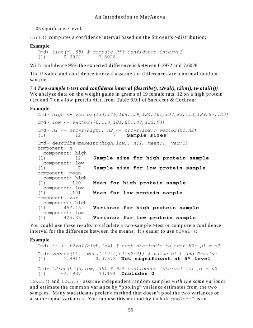
An Introduction to MacAnova
= .05 significance level.
tint() computes a confidence interval based on the Student’s t-distribution:
ExampleCmd> tint(d,.95) # compute 95% confidence interval(1) 0.3972 7.6028
With confidence 95% the expected difference is between 0.3972 and 7.6028.
The P-value and confidence interval assume the differences are a normal randomsample.
7.4 Two-sample t-test and confidence interval (describe(), t2val(), t2int(), twotailt())We analyze data on the weight gains in grams of 19 female rats, 12 on a high proteindiet and 7 on a low protein diet, from Table 6.9.1 of Snedecor & Cochran:
ExampleCmd> high <- vector(134,146,104,119,124,161,107,83,113,129,97,123)
Cmd> low <- vector(70,118,101,85,107,132,94)
Cmd> n1 <- nrows(high); n2 <- nrows(low); vector(n1,n2)(1) 12 7 Sample sizes
Cmd> describe(makestr(high,low), n:T, mean:T, var:T)component: n component: high(1) 12 Sample size for high protein sample component: low(1) 7 Sample size for low protein samplecomponent: mean component: high(1) 120 Mean for high protein sample component: low(1) 101 Mean for low protein samplecomponent: var component: high(1) 457.45 Variance for high protein sample component: low(1) 425.33 Variance for low protein sample
You could use these results to calculate a two-sample t-test or compute a confidenceinterval for the difference between the means. It’s easier to use t2val():
ExampleCmd> tt <- t2val(high,low) # test statistic to test H0: µ1 = µ2
Cmd> vector(tt, twotailt(tt,n1+n2-2)) # value of t and P-value(1) 1.8914 0.07573 Not significant at 5% level
Cmd> t2int(high,low,.95) # 95% confidence interval for µ1 - µ2(1) -2.1937 40.194 Includes 0
t2val() and t2int() assume independent random samples with the same varianceand estimate the common variance by “pooling” variance estimates from the twosamples. Many statisticians prefer a method that doesn’t pool the two variances orassume equal variances. You can use this method by include pooled:F as an
56

An Introduction to MacAnova
argument.
Cmd> result <- t2val(high,low, pooled:F); resultcomponent: t(1) 1.9107 value of t-statisticcomponent: df(1) 13.082 approximate degrees of freedom
Cmd> twotailt(result$t,result$df) # P-value(1) 0.078208
Cmd> t2int(high,low,.95,pooled:F)(1) -2.4691 40.469 Includes 0
7.5 Simple linear regression and scatter plot (regress(), plot(), secoefs(), betalimits())
Here we analyze data from Table 9.7.1 of Snedecor and Cochran which gives thepercentage of wormy fruit (pcwormy) and the number of apples harvested, in 100’s,(cropsize) for 12 apple trees. The goal is to predict or explain the amount of wormyfruit in terms of the number of applies on the tree by a simple linear regression ofpcwormy on cropsize.
Cmd> cropsize <- vector(8,6,11,22,14,17,18,24,19,23,26,40)
Cmd> pcwormy <- vector(59,58,56,53,50,45,43,42,39,38,30,27)
A first step is a scatter plot of cropsize against pcwormy.Example
Cmd> plot(pcwormy, cropsize, ymin:0,\xlab:"Percent Wormy Apples", ylab:"Crop size",title:\"Plot of crop size in 100's vs percent wormy for 12 apple trees")
0
5
10
15
20
25
30
35
40
30 35 40 45 50 55
Plot of crop size in 100's vs percent wormy for 12 apple trees
Percent Wormy Apples
Crop size
57

An Introduction to MacAnova
There is a fairly strong negative and roughly linear relationship between pcwormy andcropsize. Notice the use of keyword phrases with keywords title, xlab, ylab andymin to control the appearance of a plot. These are not really necessary, but it is alwaysa good idea to label your graphs informatively. Keyword phrase lines:T wouldconnect successive points with lines, or you could use command lineplot(). You canselect the plotting symbols used with command chplot() or by using keywordsymbols. See Sec. 6.2.
Now we do the actual regression analysis
ExampleCmd> regress("pcwormy=cropsize") # basic regression commandModel used is pcwormy=cropsize Coef StdErr tCONSTANT 64.247 3.6029 17.832cropsize -1.013 0.17215 -5.8842
N: 12, MSE: 27.384, DF: 10, R^2: 0.77590Regression F(1,10): 34.624, Durbin-Watson: 1.6899To see the ANOVA table type 'anova()
The row labelled CONSTANT pertains to the intercept and the row labeled cropsizepertains to the slope. The column headed Coef contains the least squares estimates ofthe intercept and slope. The column headed t contains t-statistics (Coef/StdErr)which can be used to test the null hypotheses that the intercept or slope is 0. You canfind the P-values using twotailt().
ExampleCmd> twotailt(vector(17.832, -5.8842), 10)(1) 6.5683e-09 0.00015431 P-values for t-stats
Both coefficients, the intercept and the slope, are significantly different from zero at the5% significance level (P-value < .05). If you include pvals:T as an argument toregress(), these P-values are printed automatically.
ExampleCmd> regress("pcwormy=cropsize",pval:T) # basic regression commandModel used is pcwormy=cropsize Coef StdErr t P-ValueCONSTANT 64.247 3.6029 17.832 6.5686e-09cropsize -1.013 0.17215 -5.8842 0.00015431
N: 12, MSE: 27.384, DF: 10, R^2: 0.77590Regression F(1,10): 34.624,P-value: 0.00015431, Durbin-Watson: 1.6899To see the ANOVA table type 'anova()'
The general usage for simple linear regression is regress("y=x"), where x and y arevectors which contain the independent and dependent variables, respectively.
After you have computed the regression, you can retrieve the coefficients and theirstandard errors using function secoefs() which computes a structure. To get just thecoefficients you can use secoefs(se:F) as an argument, while to get just the standarderrors, you can use secoefs(coefs:F):
58

An Introduction to MacAnova
ExampleCmd> secoefs() # this gets both coefficients and std. errorscomponent: CONSTANT Intercept and its standard error component: coefs(1) 64.247 component: se(1) 3.6029component: cropsize Slope and its standard error component: coefs(1) -1.013 component: se(1) 0.17215
Cmd> beta <- secoefs(se:F); ses <- secoefs(coef:F) #get separately
Cmd> # beta contains coefficients, ses contains standard Errors
Cmd> # Compute lower and upper 95% confidence limits
Cmd> n <- nrows(cropsize)# sample size
Cmd> critval <- invstu(1-.025, n-2) # Student's t critical value
Cmd> beta - critval*ses # lower confidence limitscomponent: CONSTANT(1) 56.219component: cropsize(1) -1.3966
Cmd> beta + critval*ses # upper confidence limitscomponent: CONSTANT(1) 72.275component: cropsize(1) -0.62941
You can also use macro betalimits() in file regress.mac.
ExampleCmd> betalimits(cropsize,.95) # find confidence limits for slopeWARNING: searching for unrecognized macro betalimits near betalimits((1) -1.3966 -0.62941
The warning message informs you that betalimits() was not in memory. AfterMacAnova found it and read it from file regress.mac, betalimits() computed 95%confidence limits for the slope, the coefficient of cropsize. The next time you usebetalimits() there will be no warning message.
7.6 One-way Analysis of Variance and box plot (anova(), vboxplot(), factor(), tabs())Here is a table of yields of four varieties of wheat, each grown on several plots withsimilar soils (Table 48 of Biometricheskiye Metodi of V. Yu. Urbakh, Science Press,Moscow 1964):
Variety 1 17.0 17.2 16.1 17.0 16.8
Variety 2 15.8 17.0 16.4
Variety 3 17.4 16.6 16.2 15.6 15.5 17.2
Variety 4 15.7 16.8 15.1 15.2
59

An Introduction to MacAnova
Here is a partial analysis of these data using the tabs(), vboxplot() and anova()commands. The response vector yield with final length 18 is entered in stages usingvector().
ExampleCmd> yield <- vector(17,17.2,16.1,17,16.8) # enter yield data,
Cmd> yield <- vector(yield,15.8,17,16.4) # making one long vector
Cmd> yield <- vector(yield,17.4,16.6,16.2,15.6,15.5,17.2)
Cmd> yield <- vector(yield,15.7,16.8,15.1,15.2)
Cmd> #Now generate variety numbers as another vector of length 18
Cmd> variety <- factor(rep(run(4), vector(5,3,6,4)))
Cmd> # 5, 3, 6 and 4 are the sample sizes
Cmd> # or variety <- vector(1,1,1,1,1,2,2,2,3,3,3,3,3,3,4,4,4,4)
Cmd> hconcat(variety, yield) # look at them together (1,1) 1 17 (2,1) 1 17.2 (3,1) 1 16.1 (4,1) 1 17 (5,1) 1 16.8 (6,1) 2 15.8 (7,1) 2 17 (8,1) 2 16.4 (9,1) 3 17.4(10,1) 3 16.6(11,1) 3 16.2(12,1) 3 15.6(13,1) 3 15.5(14,1) 3 17.2(15,1) 4 15.7(16,1) 4 16.8(17,1) 4 15.1(18,1) 4 15.2
Cmd> list(variety,yield) # variety is a factorvariety REAL 18 FACTOR with 4 levelsyield REAL 18
Cmd> tabs(yield, variety) # compute variety means and variancescomponent: mean(1) 16.82 16.4 16.417 15.7component: var(1) 0.182 0.36 0.63367 0.60667component: count(1) 5 3 6 4
Although the sample sizes are rather small, a box plot shows what is going on betterthan the numbers do.
60

An Introduction to MacAnova
ExampleCmd> vboxplot(split(yield,variety),xlab:"Yield",\
ylab:"Variety number", title:"Yield of wheat by variety")
15.5
16
16.5
17
1 2 3 4
Yield of wheat by variety
Yield
Variety number
Command boxplot() does the same, except the boxplots are oriented horizontally.
There appears to be a difference among varieties. To test for its reality, you cancompute an analysis of variance.
ExampleCmd> anova("yield=variety", fstat:T) #one-way ANOVAModel used is yield=varietyWARNING: summaries are sequential DF SS MS F P-valueCONSTANT 1 4821.6 4821.6 10487.75390 0variety 3 2.8237 0.94122 2.04730 0.15348ERROR1 14 6.4363 0.45974
For one-way ANOVA, the argument to anova() is a string of the form "response =factor", where factor was created using function factor(). Since the P-value forthe null hypothesis that all the means are the same is .15348, you cannot reject the nullhypothesis at any significance level < .15348.
Important: If you don’t use factor() to create the vector of category levels, you willget the wrong answer.
Without fstat:T in anova(), no F-statistics or P-values are printed. You couldcompute them “by hand,” because anova() creates several “side effect” variables,among them vectors SS and DF, containing the sums of squares and their degrees offreedom, respectively. You can find mean squares as SS/DF.
61

An Introduction to MacAnova
ExampleCmd> hconcat(DF,SS,SS/DF) # compare with ANOVA table (1) (2) (3)CONSTANT 1 4821.6 4821.6variety 3 2.8237 0.94122ERROR1 14 6.4363 0.45974
Cmd> MS <- SS/DF; MS # ANOVA mean squares CONSTANT variety ERROR1 4821.6 0.94122 0.45974
Cmd> f <- MS[2]/MS[3] # F-statistic
Cmd> vector(f,1-cumF(f, DF[2],DF[3])) # F statistic and P-value(1) 2.0473 0.15348
The row labels were automatically generated from the term names as part of the sideeffect variables DF and SS.
7.7 Randomized Block (Two-way) Analysis of Variance (anova(), factor(), tabs())Here are data from Table 14.2.1 of Snedecor and Cochran from an experiment in whichfour seed treatments and a check (no treatment) were compared in a randomized blockdesign with 4 replicates. The response is the percentage of seedlings in each plot thatfailed to emerge.
Block Number
Treatment 1 2 3 4 5
Check 8 10 12 13 11
Arasan 2 6 7 11 5
Spergon 4 10 9 8 10
Semasan,Jr 3 5 9 10 6
Fermate 9 7 5 5 3
First, enter the data as one long vector, treatment by treatment (row by row). Thencreate factors containing the replicate numbers and treatment numbers.
ExampleCmd> failures <- vector(8,10,12,13,11, 2,6,7,11,5,\
4,10,9,8,10, 3,5,9,10,6, 9,7,5,5,3)
Cmd> reps <- factor(rep(run(5),5))#vector(1,2,3,4,5,1,2,3,4,5,...,)
Cmd> treatment<-factor(rep(run(5),rep(5,5)))#vector(1,1,1,1,1,2,..)
62

An Introduction to MacAnova
Cmd> hconcat(reps, treatment, failures) # see them all (1,1) 1 1 8 (2,1) 2 1 10 (3,1) 3 1 12 (4,1) 4 1 13 (5,1) 5 1 11 (6,1) 1 2 2 (7,1) 2 2 6 (8,1) 3 2 7 (9,1) 4 2 11(10,1) 5 2 5(11,1) 1 3 4(12,1) 2 3 10(13,1) 3 3 9(14,1) 4 3 8(15,1) 5 3 10(16,1) 1 4 3(17,1) 2 4 5(18,1) 3 4 9(19,1) 4 4 10(20,1) 5 4 6(21,1) 1 5 9(22,1) 2 5 7(23,1) 3 5 5(24,1) 4 5 5
Cmd> tabs(failures,treatment,mean:T,count:T) # treatment meanscomponent: mean(1) 10.8 6.2 8.2 6.6 5.8component: count(1) 5 5 5 5 5
Cmd> tabs(failures, reps, mean:T,count:T) # block meanscomponent: mean(1) 5.2 7.6 8.4 9.4 7component: count(1) 5 5 5 5 5
Cmd> anova("failures = reps + treatment",fstat:T) # do ANOVAModel used is failures = reps + treatment DF SS MS F P-valueCONSTANT 1 1413.8 1413.8 261.32348 2.4752e-11reps 4 49.84 12.46 2.30314 0.1032treatment 4 83.84 20.96 3.87431 0.021886ERROR1 16 86.56 5.41
Cmd> # compute F-statistic and P-value “by hand”
Cmd> f <- (SS[3]/DF[3])/(SS[4]/DF[4]) # F-statistic
Cmd> vector(f,1 - cumF(f,DF[3],DF[4])) # F-statistic and P-value(1) 3.8743 0.021886 Significant at 5% level
The general form of anova() for a randomized block command is anova("response= blocks + treatment"), where response is the variable being analyzed, andblocks and treatments are vectors of block number and treatment number created byfunction factor(). This same method works even with incomplete blocks.
63
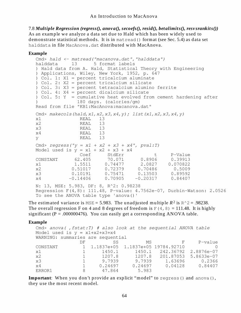
An Introduction to MacAnova
7.8 Multiple Regression (regress(), anova(), secoefs(), resid(), betalimits(), resvsrankits())As an example we analyze a data set due to Hald which has been widely used todemonstrate statistical methods. It is in matread() format (see Sec. 5.4) as data sethalddata in file MacAnova.dat distributed with MacAnova.
ExampleCmd> hald <- matread("macanova.dat","halddata")halddata 13 5 format labels) Hald data from A. Hald, Statistical Theory with Engineering) Applications, Wiley, New York, 1952, p. 647) Col. 1: X1 = percent tricalcium aluminate) Col. 2: X2 = percent tricalcium silicate) Col. 3: X3 = percent tetracalcium alumino ferrite) Col. 4: X4 = percent dicalcium silicate) Col. 5: Y = cumulative heat evolved from cement hardening after) 180 days. (calories/gm)Read from file "KB1:MacAnova:macanova.dat"
Cmd> makecols(hald,x1,x2,x3,x4,y); list(x1,x2,x3,x4,y)x1 REAL 13 x2 REAL 13 x3 REAL 13 x4 REAL 13 y REAL 13
Cmd> regress("y = x1 + x2 + x3 + x4", pval:T) Model used is y = x1 + x2 + x3 + x4 Coef StdErr t P-ValueCONSTANT 62.405 70.071 0.8906 0.39913x1 1.5511 0.74477 2.0827 0.070822x2 0.51017 0.72379 0.70486 0.5009x3 0.10191 0.75471 0.13503 0.89592x4 -0.14406 0.70905 -0.20317 0.84407
N: 13, MSE: 5.983, DF: 8, R^2: 0.98238Regression F(4,8): 111.48, P-value: 4.7562e-07, Durbin-Watson: 2.0526To see the ANOVA table type 'anova()'
The estimated variance is MSE = 5.983. The unadjusted multiple R2 is R^2 = .98238.The overall regression F on 4 and 8 degrees of freedom is F(4,8) = 111.48. It is highlysignificant (P = .000000476). You can easily get a corresponding ANOVA table.
ExampleCmd> anova( ,fstat:T) # also look at the sequential ANOVA tableModel used is y = x1+x2+x3+x4WARNING: summaries are sequential DF SS MS F P-valueCONSTANT 1 1.1837e+05 1.1837e+05 19784.92710 0x1 1 1450.1 1450.1 242.36792 2.8876e-07x2 1 1207.8 1207.8 201.87053 5.8633e-07x3 1 9.7939 9.7939 1.63696 0.2366x4 1 0.24697 0.24697 0.04128 0.84407ERROR1 8 47.864 5.983
Important: When you don’t provide an explicit “model” to regress() and anova(),they use the most recent model.
64

An Introduction to MacAnova
By default, anova() computes “sequential” sums of squares. These measure thecontribution of each variable after fitting the preceding variables, but ignoring latervariables. These are sometimes called Type I sums of squares. If you want sums ofsquares of each variable after fitting all the others (Type III sums of squares), usekeyword phrase marginal:T.
ExampleCmd> anova(,fstat:T, marginal:T)Model used is y = x1+x2+x3+x4WARNING: SS are Type III sums of squares DF SS MS F P-valueCONSTANT 1 4.7455 4.7455 0.79317 0.39913x1 1 25.951 25.951 4.33747 0.070822x2 1 2.9725 2.9725 0.49682 0.5009x3 1 0.10909 0.10909 0.01823 0.89592x4 1 0.24697 0.24697 0.04128 0.84407ERROR1 8 47.864 5.983
You can recover the coefficients and their standard errors using secoefs() andcompute critical values using invstu().
ExampleCmd> beta <- secoefs(se:F); ses <- secoefs(coef:F)
Cmd> critval <- invstu(1-.05/2,DF[6]); critval(1) 2.306 Critical value for t on 8 d.f.
Cmd> errormargins <- critval*ses
Cmd> beta - errormargins # lower limits component: CONSTANT(1) -99.179component: x1(1) -0.16634component: x2(1) -1.1589component: x3(1) -1.6385component: x4(1) -1.7791
Cmd> beta + errormargins # upper limitscomponent: CONSTANT(1) 223.99component: x1(1) 3.2685component: x2(1) 2.1792component: x3(1) 1.8423component: x4(1) 1.491
Alternatively you can use betalimits() to find confidence limits for a coefficient.Cmd> betalimits(x1, .95)(1) -0.16634 3.2685
65
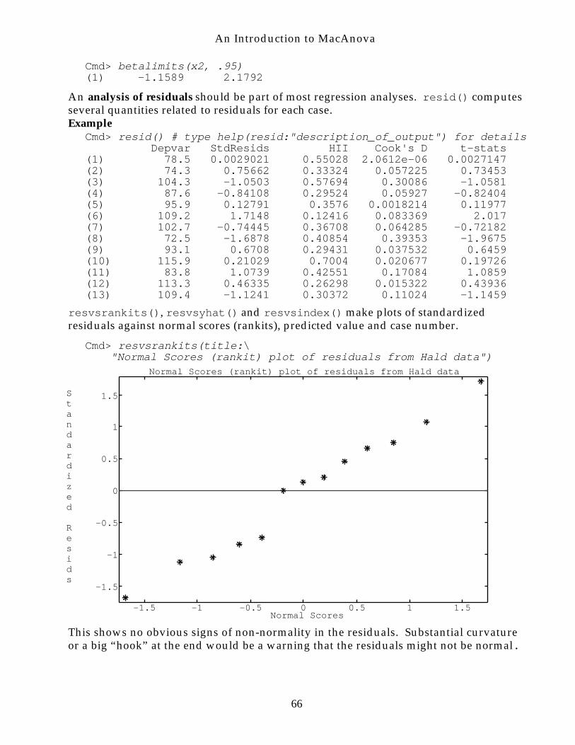
An Introduction to MacAnova
Cmd> betalimits(x2, .95)(1) -1.1589 2.1792
An analysis of residuals should be part of most regression analyses. resid() computesseveral quantities related to residuals for each case.Example
Cmd> resid() # type help(resid:"description_of_output") for details Depvar StdResids HII Cook's D t-stats(1) 78.5 0.0029021 0.55028 2.0612e-06 0.0027147(2) 74.3 0.75662 0.33324 0.057225 0.73453(3) 104.3 -1.0503 0.57694 0.30086 -1.0581(4) 87.6 -0.84108 0.29524 0.05927 -0.82404(5) 95.9 0.12791 0.3576 0.0018214 0.11977(6) 109.2 1.7148 0.12416 0.083369 2.017(7) 102.7 -0.74445 0.36708 0.064285 -0.72182(8) 72.5 -1.6878 0.40854 0.39353 -1.9675(9) 93.1 0.6708 0.29431 0.037532 0.6459(10) 115.9 0.21029 0.7004 0.020677 0.19726(11) 83.8 1.0739 0.42551 0.17084 1.0859(12) 113.3 0.46335 0.26298 0.015322 0.43936(13) 109.4 -1.1241 0.30372 0.11024 -1.1459
resvsrankits(), resvsyhat() and resvsindex() make plots of standardizedresiduals against normal scores (rankits), predicted value and case number.
Cmd> resvsrankits(title:\"Normal Scores (rankit) plot of residuals from Hald data")
-1.5
-1
-0.5
0
0.5
1
1.5
-1.5 -1 -0.5 0 0.5 1 1.5
Normal Scores (rankit) plot of residuals from Hald data
Normal Scores
Standardized Resids
This shows no obvious signs of non-normality in the residuals. Substantial curvatureor a big “hook” at the end would be a warning that the residuals might not be normal.
66
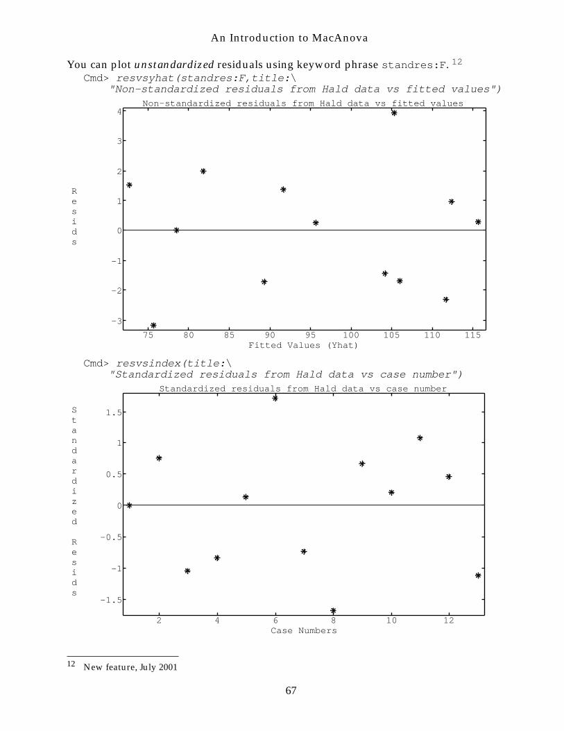
An Introduction to MacAnova
You can plot unstandardized residuals using keyword phrase standres:F. 12
Cmd> resvsyhat(standres:F,title:\"Non-standardized residuals from Hald data vs fitted values")
-3
-2
-1
0
1
2
3
4
75 80 85 90 95 100 105 110 115
Non-standardized residuals from Hald data vs fitted values
Fitted Values (Yhat)
Resids
Cmd> resvsindex(title:\"Standardized residuals from Hald data vs case number")
-1.5
-1
-0.5
0
0.5
1
1.5
2 4 6 8 10 12
Standardized residuals from Hald data vs case number
Case Numbers
Standardized Resids
12 New feature, July 2001
67