An Introduction to Information Theory

Vahid Meghdadireference : Elements of Information Theory by Cover and Thomas

September 2007

Contents

1 Entropy 2

2 Joint and conditional entropy 4

3 Mutual information 5

4 Data Compression or Source Coding 6

5 Channel capacity 85.1 examples . . . . . . . . . . . . . . . . . . . . . . . . . . . . . . . 9

5.1.1 Noiseless binary channel . . . . . . . . . . . . . . . . . . . 95.1.2 Binary symmetric channel . . . . . . . . . . . . . . . . . . 95.1.3 Binary erasure channel . . . . . . . . . . . . . . . . . . . . 105.1.4 Two fold channel . . . . . . . . . . . . . . . . . . . . . . . 11

6 Differential entropy 126.1 Relation between differential and discrete entropy . . . . . . . . . 136.2 joint and conditional entropy . . . . . . . . . . . . . . . . . . . . 136.3 Some properties . . . . . . . . . . . . . . . . . . . . . . . . . . . . 14

7 The Gaussian channel 157.1 Capacity of Gaussian channel . . . . . . . . . . . . . . . . . . . . 157.2 Band limited channel . . . . . . . . . . . . . . . . . . . . . . . . . 167.3 Parallel Gaussian channel . . . . . . . . . . . . . . . . . . . . . . 18

8 Capacity of SIMO channel 19

9 Exercise (to be completed) 22

1

1 Entropy

Entropy is a measure of uncertainty of a random variable. The uncertainty orthe amount of information containing in a message (or in a particular realizationof a random variable) is defined as the inverse of the logarithm of its probabil-ity: log(1/PX(x)). So, less likely outcome carries more information. Let Xbe a discrete random variable with alphabet X and probability mass functionPX(x) = Pr{X = x}, x ∈ X . For convenience PX(x) will be denoted by p(x).The entropy of X is defined as follows:

Definition 1. The entropy H(X) of a discrete random variable is defined by

H(X) = E log1

p(x)

=∑x∈X

p(x) log1

p(x)(1)

Entropy indicates the average information contained in X. When the baseof the logarithm function is 2, the entropy is measured in bits. For example theentropy of a fair coin toss is 1 bit.Note: The entropy is a function of the distribution of X. It does not depend onthe actual values taken by the random variable, but only on the probabilities.note: H(X) ≥ 0.

Example 1. : Let

X ={

1 with probability p0 with probability 1− p (2)

Show that the entropy of X is

H(X) = −p log p− (1− p) log(1− p) (3)

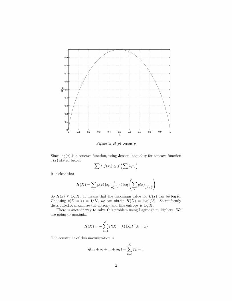
Some times this entropy is denoted by H(p, 1 − p). Note that the entropy ismaximized for p = 0.5 and it is zero for p = 1 or p = 0. This makes sense becausewhen p = 0 or p = 1 there is no uncertainty over the random variable X andhence no information in revealing its outcome. The maximum uncertainty iswhen the two events are equi-probable.

Example 2. : Suppose X can take on K values. Show that that the entropyis maximized when X is uniformly distributed on these K Values and in thiscase, H(X) = logK.

Solution: Calculating H(X) results in:

H(X) =K∑x=1

p(x) log1

p(x)

2

0 0.1 0.2 0.3 0.4 0.5 0.6 0.7 0.8 0.9 10

0.1

0.2

0.3

0.4

0.5

0.6

0.7

0.8

0.9

1

p

H(p

)

Figure 1: H(p) versus p

Since log(x) is a concave function, using Jenson inequality for concave functionf(x) stated below: ∑

λif(xi) ≤ f(∑

λixi

)it is clear that

H(X) =∑x

p(x) log1

p(x)≤ log

(∑x

p(x)1

p(x)

)

So H(x) ≤ logK. It means that the maximum value for H(x) can be logK.Choosing p(X = i) = 1/K, we can obtain H(X) = log 1/K. So uniformlydistributed X maximize the entropy and this entropy is logK.

There is another way to solve this problem using Lagrange multipliers. Weare going to maximize

H(X) = −K∑k=1

P (X = k) logP (X = k)

The constraint of this maximization is

g(p1 + p2 + ...+ pK) =K∑k=1

pk = 1

3

So by changing pi we try to find the maximum point of H. For all k from 1 toK we should maximize

H + λ(g − 1)

Hence we require:∂

∂pk(H + λ(g − 1)) = 0

It means that:

∂

∂pk

(−

K∑k=1

p(k) log p(k) + λ(K∑k=1

pk − 1)

)= 0

After calculating the differentiation we obtain a set of K independent equa-tions as:

−(

1ln 2

+ log2 pk

)+ λ = 0

Solving this equation, we remark that all the pk have the same value. So the

pk =1K

As a conclusion, the uniform distribution yields the greatest entropy.

2 Joint and conditional entropy

We saw the entropy of a single random variable (RV) and we now extend it toa pair of RV.

Definition 2. The joint entropy H(X,Y ) of a pair of discrete random variables(X,Y ) with a joint distribution p(x, y) is defined as:

H(X,Y ) = −∑x∈X

∑y∈Y

p(x, y) log p(x, y) (4)

which can also be expressed as

H(X,Y ) = −E log p(X,Y ) (5)

The conditional entropy is defined at the same way. It is the expectation ofthe entropies of the conditional distributions:

4

Definition 3. If (X,Y ) ∼ p(x, y), then the conditional entropy H(Y |X) isdefined as:

H(Y |X) =∑x∈X

p(x)H(Y |X = x) (6)

= −∑x∈X

p(x)∑y∈Y

p(y|x) log p(y|x) (7)

= −∑x∈X

∑y∈Y

p(x, y) log p(y|x) (8)

= Ep(x,y) log p(Y |X) (9)

Theorem 1. (chain rule)

H(X,Y ) = H(X) +H(Y |X) (10)

The proof comes from the fact that

log p(X,Y ) = log p(X) + log p(Y |X)

and then take the expectation.

3 Mutual information

The mutual information is a measure of the amount of information that onerandom variable contains about another random variable. It is the reduction ofuncertainty of one random variable due to the knowledge of the other. It is:

I(X;Y ) = H(X)−H(X|Y ) (11)

= Ep(x,y) logp(X,Y )p(X)p(Y )

(12)

= H(Y )−H(Y |X) (13)= I(Y ;X) (14)

The diagram of figure 2 represents the relation between the conditional entropiesand mutual information.

The chain rule can be stated here for the mutual information. First we definethe conditional mutual information as:

I(X;Y |Z) = H(X|Z)−H(X|Y,Z) (15)

Using this definition the chain rule can be written.

I(X1, X2;Y ) = H(X1, X2)−H(X1, X2|Y ) (16)= H(X1) +H(X2|X1)−H(X1|Y )−H(X2|X1, Y ) (17)= I(X1;Y ) + I(X2;Y |X1) (18)

5

H ( Y | X )H ( X | Y ) I ( X ; Y )

Figure 2: Relation between entropy and mutual information

Some properties

•I(X;Y ) ≥ 0

•I(X;Y |Z) ≥ 0

• H(X) ≤ log |X | where |X | denotes the number of elements in the range ofX, with the equality if and only if X has a uniform distribution over X .

• Condition reduces entropy:

H(X|Y ) ≤ H(X)

with equality if and only if X and Y are independent.

• H(X1, X2, . . . , Xn) ≤∑ni=1H(Xi) with equality if and only if the Xi are

independent.

• Let (X,Y ) ∼ p(x, y) = p(x)p(y|x). The mutual information I(X;Y ) is aconcave function of p(x) for fixed p(y|x) and a convex function of p(y|x)for fixed p(x).

4 Data Compression or Source Coding

Two classes of coding are used: lossless source coding and lossy source coding.In this section, only lossless coding will be considered. The data compressioncan be achieved by assigning short descriptions to the most frequent outcomesof data source and then longer to the less probable. For example in Morse code,the letter ”e” is coded by just a point.

In this chapter some principles of compression will be given.

Definition 4. A source code C for a random variable X is a mapping from X ,the range of X, to D, the set of finite length strings of symbols from a D-aryalphabet. Let C(x) denote the codeword corresponding to x and let l(x) denote

6

the length of C(x).

Example 3. : If you toss a coin, X = {tail, head}, C(head) = 0, C(tail) =11, l(head) = 1, l(tail) = 2.

Definition 5. The expected length of a code C(x) for a random variable Xwith probability mass function p(x) is given by

L(C) =∑x∈X

p(x)l(x) (19)

For example for the above example the expected length of the code is

L(C) =12∗ 2 +

12∗ 1 = 1.5

Definition 6. The code is singular if C(x1) = C(x2) and x1 6= x2.

Non singular codes are uniquely decodable.

Definition 7. The extension of a code C is a code obtained as:

C(x1x2 . . . xn) = C(x1)C(x2) . . . C(xn) (20)

It means that a long message can be coded by concatenating the shorter mes-sage code words. For example if C(x1) = 11 and C(x2) = 00, then C(x1x2) =1100.

Definition 8. A code is uniquely decodable if its extension is non-singular.

In other words, any encoded string has only one possible source string andthere is no ambiguity.

Definition 9. A code is called a prefix code or an instantaneous code if no codeword is a prefix of any other codeword.

Example 4. The following code is a prefix code: C(x1) = 1, C(x2) = 01, C(x3) =001, C(X4) = 000. Any encoded sequence is uniquely decodable and its corre-sponding source word can be obtained as soon as the code word is received.In other word, an instantaneous code can be decoded without reference to thefuture codewords since the end of a codeword is immediately recognizable. Forexample the sequence 001100000001 is decoded as x3x1x4x4x2.

Example 5. The following code is not instantaneous code but uniquely de-codable: C(x1) = 1, C(x2) = 10, C(x3) = 100, C(X4) = 000. Why? Here youshould wait to receive a 1 to be able to decode.Note that if we look at the encoded sequence from right to left, it becomesinstantaneous.

Figure 3 illustrates the different nesting of codes.

7

A l l c o d e s

N o n - s i n g u l a r c o d e

U n i q u e l y d e c o d a b l e c o d e s

I n s t a n t a n e o u s c o d e s

Figure 3: Classes of codes

5 Channel capacity

Assume that we have a channel whose input is the random variable X with inputalphabet {0, 1, 2, 3} and output alphabet {A,B,C,D}, as presented in Figure4. The goal is to send the information without error. If we send 2 bits per inputsymbol, there is no way to determine precisely which symbol was sent. However,if we use less rate, for example just one bit per channel use it is possible to sendinformation without error. In this case we use only the symbols 0 and 2 (or 1and 3) and at the channel output we can precisely determine the symbol sent.It means by reducing the rate, reliable transmission is possible. What we didis to modify the PX(x) to maximize the rate and at the same time to obtaina reliable communication. In this example P (X = 0) = P (X = 2) = 0.5 andP (X = 1) = P (X = 3) = 0.In this way we proposed a scheme that achieves 1 bit per channel use. Is it themaximum that we can obtain? The answer is yes because H(Y ) is the entropyof Y which is at most equal to 2 (there are 4 possibilities), so H(Y ) ≤ 2. Theconditional entropy H(Y |X) explains the uncertainty over Y given X. But ifX is known, there is two equi-probable possibilities for Y giving this entropyequals to 1. So

[H(Y )−H(Y |X)] ≤ 2− 1 = 1

Therefor the information rate cannot be greater than 1, so the scheme proposedis optimal.Note: If we reduce the rate below a certain number, reliable communicationcan be obtained.

Definition 10. The channel capacity of a discrete memoryless channel is de-fined as:

C = maxp(x)

I(X;Y )

= maxp(x)

[H(Y )−H(Y |X)] (21)

8

Figure 4: Noisy channel

5.1 examples

5.1.1 Noiseless binary channel

Consider the channel presented in Figure 5. Show that the capacity is 1 bit persymbol (or per channel use).

Figure 5: Ideal channel

5.1.2 Binary symmetric channel

For the binary symmetric channel (BSC) of Figure 6 show that the capacity is

CBSC = 1−H(p, 1− p) (22)

This channel is equivalent to a channel with Y = X ⊕ Z where

Z ={

1 prob p0 prob 1− p

Figure 6: BSC channel

9

and X and Z are independent. We can say that H(Y |X) = H(Z) because whenX is given, knowing Y is the same as knowing Z. At the output, Y has onlytwo possibilities, so we can say H(Y ) ≤ 1. Maximum is achievable by choosingPX(0) = PX(1) = 1/2. So I(X;Y ) ≤ 1 − H(Z). The capacity should be:CBSC = 1−H(p, 1− p).

Exercise

We are using a continuous AWGN channel where the input is a random variableX ∈ {3,−3} and the noise is Gaussian with N ∼ N (0, 1). The channel outputis: Y = X +N . We want to calculate the capacity.Note: The capacity is not log(1 + SNR) because the distribution of X is notoptimized (the capacity maximizing distribution in this case is Gaussian whilehere, X can only take two values).Hint: Put a threshold at 0 and then calculate the probability of error. Thechannel is now BSC and you can use the results given in this section. Note thatthe capacity of this channel supposing that the noise variance goes to zero (highSNR) cannot be greater than 1 bit per channel use.

5.1.3 Binary erasure channel

The binary erasure channel is when some bits are lost (rather than corrupted).Here the receiver knows which bit has been erased. Figure 7 shows this channel.We are to calculate the capacity of binary erasure channel.

C = maxp(x)

I(X;Y )

= maxp(x)

[H(Y )−H(Y |X)]

= maxp(x)

[H(Y )−H(a, 1− a)] (23)

Because of the symmetry we assume that P (X = 0) = P (X = 1) = 1/2. So Yhave three possibilities with probabilities P (Y = 0) = P (Y = 1) = (1 − a)/2and P (Y = e) = a. So we can write:

C = H

(1− a

2,

1− a2

, a

)−H(a, 1− a)

= 1− a bit per channel use (24)

How to attain this capacity? If there is a feedback from the receiver, eachtime an erasure is detected, the receiver asks the transmitter to resend the erasedbit. Because of the erasure probability of a, it happens to repeat a symbol onceevery 1/a symbols. This means that for a large sequence of N symbols sent (orN channel use) only N − aN information bits are passed to the receiver. Sowith this structure the rate 1− a bit per channel use is achieved.However, it can be proved that this rate is the maximal rate even if there is nofeedback. In fact, feedback does not increase the capacity of discrete memorylesschannels.

10

Figure 7: Erasure channel

5.1.4 Two fold channel

Suppose we have two independent memoryless channels drawn in Figure 8. Sup-pose also that the receiver knows which of the channels is used. The transmitteruses the channel following the symbol to be transmitted. In other word, twodifferent alphabets are used for channels 1 and 2. We are to calculate the ca-pacity of the channel: max I(X;Y ).Let’s define a new variable S as:

Figure 8: Two channel configuration

S ={

1 if channel 1 is used with prob a2 if channel 2 is used with prob 1− a

We have I(X;Y ) = I(X;Y, S). This is because the received alphabet are dis-tinct so knowing Y implies that we know S. However to prove this, using chainrule we can write: I(X;Y, S) = I(X;Y ) + I(X;S|Y ). The second term isH(S|Y )−H(S|Y,X) which is equal to zero because if we know Y we know S.So the above equation is proved.Developing the above relation we have:

I(X;Y ) = I(X;Y, S)= I(X;S) + I(X;Y |S)= H(S)−H(S|X) + I(X;Y |S = 1)P (S = 1) + I(X;Y |S = 2)P (S = 2)= H(a, 1− a) + 0 + I(X;Y1)a+ I(X;Y2)(1− a)

11

To maximize the mutual information with respect to a, PX1 , PX2 , we calculatethe derivative equals to zero with respect to a, which gives:

a =2C1

2C1 + 2C2

Replacing this value in I we obtain:

C = log2(2C1 + 2C2) (25)

6 Differential entropy

In this section we consider continuous random variables rather than discrete ran-dom variables. The entropy as defined before uses the probability mass functionand does not work here. Instead, we use the probability density function (PDF)to define the entropy of X.

Definition 11. The random variable X is said to be continuous if its cumulativedistribution function F (x) = Pr(X ≤ x) is continuous.

Definition 12. The differential entropy h(X) of a continuous random variableX with a PDF PX(x) is defined as

h(X) =∫S

PX(x) log1

PX(x)dx

= E[log

1PX(x)

](26)

where S is the support set of the random variable.

Uniform distribution

Show that for X ∼ U(0, a) the differential entropy is log a. Note that unlikediscrete entropy, the differential entropy can be negative. However, 2h(X) =2log a = a is the volume of the support set, which is always non-negative, asexpected.

Normal distribution

Show that for X ∼ N (0, σ2) the differential entropy is

h(x) =12

log(2πeσ2) bits (27)

Exponential distribution

Show that for PX(x) = λe−λx for X ≥ 0 the differential entropy is

h(x) = loge

λbits (28)

What is the entropy if PX(x) = λ2 e−λ|x|?

12

6.1 Relation between differential and discrete entropy

Referring to the Figure 9, the continuous random variable X is quantized togenerate a discrete random variable denoted by X∆. This random variabletakes the value xi if i∆ ≤ X ≤ (i+ 1)∆. Then the probability that X∆ = xi is

pi =∫ (i+1)∆

i∆

PX(x)dx (29)

Figure 9: Quantization of a continuous random variable

Now, because X∆ is a discrete random variable,m we can write the discreteentropy as:

H(X∆) = −∞∑−∞

pi log pi

= −∞∑−∞

PX(xi)∆ log(PX(xi)∆)

= −∑

∆PX(xi) logPX(xi)− log ∆ (30)

and as ∆→ 0 we can write:

H(X∆) + log ∆→ h(X) (31)

The important result is the entropy of an n-bit quantization of a continuousrandom variable X is approximately h(X) + n.

6.2 joint and conditional entropy

The differential entropy can be extended to several random variables. so:

h(X1, X2, ..., Xn) = −∫p(x1, x2, ..., xn) log p(x1, x2, ..., xn)dx1dx2...dxn (32)

13

h(X|Y ) = −∫p(x, y) log p(x|y)dxdy (33)

= h(X,Y )− h(Y ) (34)

Theorem 2. (Entropy of multivariate normal distribution): Let X be a randomnormal vector with mean vector µ and covariance matrix K. Then

h(X1, X2, ..., Xn) =12

log ((2πe)n|K|) bits (35)

Note that the mean of the distribution has no effect on entropy. In general:

h(Y ) = h(Y + cte)

6.3 Some properties

• Chain rule h(X,Y ) = h(X) + h(Y |X)

• Uncorrelated Gaussian random vectorX = [X1X2...Xn]T withX1, X2, ..., Xn

i.i.d. ∼ N (0, 1)

h(X) =12

log(2πe)n

• Given a random vector X with h(X), the differential entropy of the randomvector Y = AX will be

h(Y) = h(X) + log |A|

• The same case but for scalar random variable. If Y = cX, we have h(Y ) =h(X)+log |c|. Note: For discrete random variables if Y = cX, the entropyof X and Y are the same: H(X) = H(Y ).

Theorem 3. Suppose X is a random vector with E(X) = 0 and E(XXT ) = K,then h(X) ≤ 1

2 log(2πe)n|K|. The equality is achieved only if X is Gaussian∼ N (0,K)

Application (Hadamard’s inequality)

Let X ∼ N (0,K) be a multi-variant normal random variable, then the Hadamardinequality states that:

|K| =n∏i=1

Kii

14

Proof. Using chain rule, we can write:

h(X) = h(X1) + h(X2|X1) + h(X3|X1, X2) + · · ·+ h(Xn|X1, · · · , Xn)12

log(2πe)n|K| ≤ h(X1) + h(X2) + · · ·+ h(Xn)

=12

log(2πe)K11 +12

log(2πe)K22 + · · ·+ 12

log(2πe)Knn

=12

log(2πe)nK11K22 · · ·Knn

7 The Gaussian channel

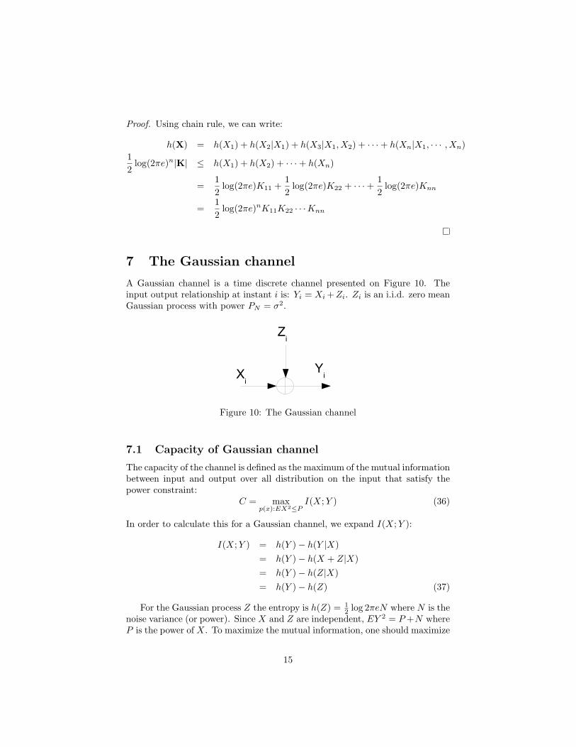
A Gaussian channel is a time discrete channel presented on Figure 10. Theinput output relationship at instant i is: Yi = Xi +Zi. Zi is an i.i.d. zero meanGaussian process with power PN = σ2.

Figure 10: The Gaussian channel

7.1 Capacity of Gaussian channel

The capacity of the channel is defined as the maximum of the mutual informationbetween input and output over all distribution on the input that satisfy thepower constraint:

C = maxp(x):EX2≤P

I(X;Y ) (36)

In order to calculate this for a Gaussian channel, we expand I(X;Y ):

I(X;Y ) = h(Y )− h(Y |X)= h(Y )− h(X + Z|X)= h(Y )− h(Z|X)= h(Y )− h(Z) (37)

For the Gaussian process Z the entropy is h(Z) = 12 log 2πeN where N is the

noise variance (or power). Since X and Z are independent, EY 2 = P+N whereP is the power of X. To maximize the mutual information, one should maximize

15

h(Y ) with the power constraint of PY = P + N . We saw that the distributionmaximizing the entropy for a continuous random variable is Gaussian. This canbe obtain if X is Gaussian. Applying this to the mutual information formula(37), we obtain

I(X;Y ) = h(Y )− h(Z)

≤ 12

log 2πe(P +N)− 12

log 2πeN

=12

log(

1 +P

N

)(38)

Hence the information capacity of a Gaussian channel is

C = maxp(x):EX2≤P

I(X;Y ) =12

log(

1 +P

N

)(39)

and this maximum is attained when X ∼ N (0, P ).

Example 6. What is the capacity of the following transmission system:

Y = 3X + N

where E X2 ≤ Px and N ∼ N (0, PN ).Let X′ = 3X so PX′ ≤ 9Px and the capacity of this channel will be:

C =12

log(1 +9PxPN

)

Therefore the capacity is increased. Here the channel gain is a deterministicvalue and the channel is flat.

7.2 Band limited channel

Suppose we have a continuous channel with bandwidth B and the power spectraldensity of noise is N0/2. So the analog noise power is N0B. On the other hand,supposing that the channel is used over the time interval [0, T ]. So the power ofanalog signal times T gives the total energy of the signal in this period. UsingShannon sampling theorem, there are 2B samples per second. So the power ofdiscrete signal per sample will be PT/2BT = P/2B. The same argument canbe used for the noise, so the power of samples of noise is N0

2 2B T2BT = N0/2. So

the capacity of the Gaussian channel per sample is:

C =12

log(

1 +P

N0B

)bits per sample (40)

Since there are maximum 2B independent samples per second the capacitycan be written as:

C = B log(

1 +P

N0B

)bits per second (41)

16

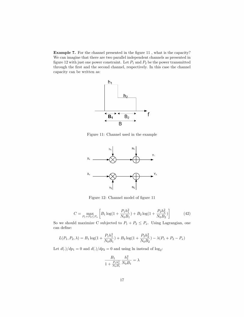
Example 7. For the channel presented in the figure 11 , what is the capacity?We can imagine that there are two parallel independent channels as presented infigure 12 with just one power constraint. Let P1 and P2 be the power transmittedthrough the first and the second channel, respectively. In this case the channelcapacity can be written as:

Figure 11: Channel used in the example

Figure 12: Channel model of figure 11

C = maxP1+P2≤Px

[B1 log(1 +

P1h21

N0B1) +B2 log(1 +

P2h22

N0B2)]

(42)

So we should maximize C subjected to P1 + P2 ≤ Px. Using Lagrangian, onecan define:

L(P1, P2, λ) = B1 log(1 +P1h

21

N0B1) +B2 log(1 +

P2h22

N0B2)− λ(P1 + P2 − Px)

Let d(.)/dp1 = 0 and d(.)/dp2 = 0 and using ln instead of log2:

B1

1 + P1h21

N0B1

h21

N0B1= λ

17

P1

B1N0=

1λN0

− 1h2

1

With the same operations we obtain:

P1

B1N0= Cst− 1

h21

(43)

P2

B2N0= Cst− 1

h22

(44)

Where the Cte can be found by setting P1 + P2 = Px. Since the two powersare found, the capacity of the channel is calculated using equation 42. The onlyconstraint that to be considered is that P1 and P2 cannot be negative. If one ofthese is negative, the corresponding power is zero and all the power are assignedto the other one. This principle is called water filling.

Exercise 1. Use the same principle (water filling) and give the power allocationfor a channel with three frequency bands defined as follows: h1 = 1/2, h2 = 1/3and h3 = 1; B1 = B, B2 = 2B and B3 = B; Px = P1 + P2 + P3 = 10.solution: P1 = 3.5, P2 = 0 and P3 = 6.5.

7.3 Parallel Gaussian channel

Here we consider k independent Gaussian channels in parallel with a commonpower constraint as depicted in Figure 13. The objective is to maximize thecapacity by optimal distribution of the power among the channels:

C = maxpX1,...,Xk

(x1,...,xk):∑EX2

i≤PI(X1, ..., Xk;Y1, ..., Yk) (45)

Figure 13: Parallel Gaussian channels

18

Using the independence of Z1, ..., Zk:

C = I(X1, ..., Xk;Y1, ..., Yk)= h(Y1, ..., Yk)− h(Y1, ..., Yk|X1, ..., Xk)= h(Y1, ..., Yk)− h(Z1, ..., Zk)

≤∑i

h(Yi)− h(Zi)

≤∑i

12

log(

1 +PiNi

)

8 Capacity of SIMO channel

Consider the channel presented in figure 14. X is a binary random variablewith Px(1) = Px(0) = 1/2. Z1 and Z2 are two binary random variables (i.i.d)representing the effect of channel noise with P (Z1 = 1) = P (Z2 = 1) = p. Thecapacity of the channel is C1 = I(X; (Y1, Y2)). We can add a data processingunit at the output as presented in figure 15. Now the whole channel is calledC2. We can write for Z the following equation.

Figure 14: SIMO channel

Figure 15: SIMO channel with data processing

19

Z =

1 if Y1 = Y2 = 10 if Y1 = Y2 = 0ε1 if Y1 = 1, Y2 = 0ε2 if Y1 = 0, Y2 = 1

The capacity of C2 can be calculated using the probabilities P (Z|X). Alsowith the same principle the capacity of C1 can be calculated. But which one isgreater C1 or C2?First C2 cannot be greater than C1, it means that C1 ≥ C2; that is becausesignal processing cannot increase the capacity. Second, here, there is no lossof information because of signal processing. It means that the processing iscompletely invertible: (Y1, Y2)⇔ Z. So C1 = C2.But if we had as data processing the following relation:

Z =

1 if Y1 = Y2 = 10 if Y1 = Y2 = 0ε if Y1 6= Y2

Here there is some information loss, what we can say in this case? First asbefore C1 ≥ C2. Here we are not interested in Y but in X. So the two channelsare equivalent. This can be shown mathematically.

I(X;Y1, Y2, Z) = I(X;Y1, Y2) + I(X;Z|Y1, Y2)

This is because I(A;B,C) = I(A;B) + I(A;C|B). The first term in the aboveequation is the capacity of the first channel and the second term is equal to zerobecause if you know Y 1 and Y2 you know perfectly Z. We can also write:

I(X;Y1, Y2, Z) = I(X;Z) + I(X;Y1, Y2|Z)

The first term is the capacity of the second channel. If we show that the secondterm is zero, we have shown that C1 = C2. We can say:

I(X;Y1, Y2|Z) = P (Z = 0)I(X;Y1, Y2|Z = 0)+ P (Z = 1)I(X;Y1, Y2|Z = 1)+ P (Z = ε)I(X;Y1, Y2|Z = ε)

Since there is no information on Y1 and Y2 when Z = 0 or Z = 2, we can write:

I(X;Y1, Y2|Z) = P (Z = ε)I(X;Y1, Y2|Z = ε)= P (Z = ε)[H(Y1, Y2|Z = ε)−H(Y1, Y2|Z = ε,X)]

It can be shown that the two terms are equal to one which gives zero as theresult. It means that we have shown C1 = C2. So Z has all information of X;it is a sufficient statistics for X.We are now interested in Gaussian variables resulting from Gaussian channels.

20

Suppose X ∼ N (0, P ), N1 ∼ N (0, 1) and N2 ∼ N (0, 1). N1 and N2 are jointlyi.i.d Gaussian random variable.

Y1 = X + Z1

Y2 = X + Z2

Y =[Y1

Y2

]=[X + Z1

X + Z2

]= X + Z

The random variable Z is defined as Z = Y1 +Y2. It means that the signal pro-cessing unit is an addition block (here it is called maximum ration combiner).Is there any loss of information here?To prove this, we construct the variable Y from the following invertible trans-formation.

Y =[

1 1−1 1

] [Y1

Y2

]=[Y1

Y2

]The question is that with this process is the capacity will be the same? First ofall the processing cannot increase the capacity. Since the process is invertiblethere is no information loss. It means that I(X; Y) = I(X; Y).

Y =[

Y1 + Y2

−Y1 + Y2

]=[

Z−Z1 + Z2

]=[

2X + Z1 + Z2

−Z1 + Z2

]We can show that Z1 +Z2 is independent of −Z1 +Z2. That is because the twoare Gaussian and uncorrelated:

E((Z2 + Z1)(Z2 − Z1)) = 0

So we can write:

I(X; Y) = I(X; Y) = I(X; Y1, Y2) = I(X; Y1) + I(X; Y2|Y1)

and

I(X; Y2|Y1) = I(X;−Z1 + Z2|2X + Z1 + Z2)= H(−Z1 + Z2|2X + Z1 + Z2)−H(−Z1 + Z2|2X + Z1 + Z2, X)= 0

This is true because on independence of Z1 + Z2 and Z2 − Z1. Therefore;

I(X; Y) = I(X;Z)

So Z is sufficient statistic for X.

21

9 Exercise (to be completed)

1. Let

X =

a with probability 1/2,b with probability 1/4,c with probability 1/8,d with probability 1/8,

What is entropy of X ? (answer: 7/4 bits)Suppose we wish to determine the value of X with the minimum number ofbinary question. What is an efficient questions ? What is the expectationvalue of the number of questions ? (answer: 1.75)

22