an introduction to dynamic games a. haurie j. b....
TRANSCRIPT

An Introduction to Dynamic Games
A. Haurie
J. B. Krawczyk

Contents
Chapter I. Foreword 5I.1. What aredynamic games? 5I.2. Origins of this book 5I.3. What is different in this presentation 6
Part 1. Foundations of Classical Game Theory 7
Chapter II. Elements of Classical Game Theory 9II.1. Basic concepts of game theory 9II.2. Games in extensive form 10II.3. Additional concepts about information 15II.4. Games in normal form 17II.5. Exercises 20
Chapter III. Solution Concepts for Noncooperative Games 23III.1. Introduction 23III.2. Matrix games 24III.3. Bimatrix games 32III.4. Concavem-person games 38III.5. Correlated equilibria 45III.6. Bayesian equilibrium with incomplete information 49III.7. Appendix on Kakutani fixed-point theorem 53III.8. Exercises 53
Chapter IV. Cournot and Network Equilibria 57IV.1. Cournot equilibrium 57IV.2. Flows on networks 61IV.3. Optimization and equilibria on networks 62IV.4. A convergence result 69
Part 2. Repeated and sequential Games 73
Chapter V. Repeated Games and Memory Strategies 75V.1. Repeating a game in normal form 76V.2. Folk theorem 79V.3. Collusive equilibrium in a repeated Cournot game 82V.4. Exercises 85
Chapter VI. Shapley’s Zero Sum Markov Game 87VI.1. Process and rewards dynamics 87
3

4 CONTENTS
VI.2. Information structure and strategies 87VI.3. Shapley’s-Denardo operator formalism 89
Chapter VII. Nonzero-sum Markov and Sequential Games 93VII.1. Sequential games with discrete state and action sets 93VII.2. Sequential games on Borel spaces 95VII.3. Application to a stochastic duopoloy model 96
Index 101
Bibliography 103

CHAPTER I
Foreword
I.1. What are dynamic games?
Dynamic Gamesare mathematical models of the interaction between indepen-dent agents who are controlling a dynamical system. Such situations occur in militaryconflicts (e.g.,duel between a bomber and a jet fighter), economic competition (e.g.,investments in R&D for computer companies), parlor games (chess, bridge). Theseexamples concern dynamical systems since the actions of the agents (also called play-ers) influence the evolution over time of thestateof a system (position and velocityof aircraft, capital of know-how for Hi-Tech firms, positions of remaining pieces ona chess board, etc). The difficulty in deciding what should be the behavior of theseagents stems from the fact that eachactionan agent takes at a given time will influencethe reaction of theopponent(s)at later time. These notes are intended to present thebasic concepts and models which have been proposed in the burgeoning literature ongame theory for a representation of these dynamic interactions.
I.2. Origins of this book
These notes are based on several courses onDynamic Gamestaught by the au-thors, in different universities or summer schools, to a variety of students in engineer-ing, economics and management science. The notes use also some documents preparedin cooperation with other authors, in particular B. Tolwinski [63] and D. Carlson.
These notes are written forcontrol engineers, economistsor management scien-tists interested in the analysis of multi-agent optimization problems, with a particularemphasis on the modeling of competitive economic situations. The level of mathemat-ics involved in the presentation will not go beyond what is expected to be known bya student specializing in control engineering, quantitative economics or managementscience. These notes are aimed at last-year undergraduate, first year graduate students.
The Control engineers will certainly observe that we presentdynamic gamesas anextension ofoptimal whereas economists will see also thatdynamic gamesare onlya particular aspect of theclassical theory of gameswhich is considered to have beenlaunched by J. Von Neumann and O. Morgenstern in the 40’s1. The economic models
1The book [66] is an important milestone in the history of Game Theory.
5
6 I. FOREWORD
of imperfect competition that we shall repeatedly use as motivating examples, have amore ancient origin since they are all variations on the original Cournot model [10],proposed in the mid 18-th century . An interesting domain of application ofdynamicgames, which is described in these notes, relates to environmental management. Theconflict situations occurring in fisheries exploitation by multiple agents or in policy co-ordination for achieving global environmental (e.g.,in the control of a possible globalwarming effect) are well captured in the realm of this theory.
The objects studied in this book will bedynamic. The termdynamic comes fromGreekδυναµικωσ [powerful] , δυναµισ [power], [strength] and meansof or pertaining to force producing motion2. In an every day context,dynamic isan attribute of a phenomenon that undergoes a time-evolution. So, in broad terms,dynamic systems are such that change in time. They may evolve “endogenously” likeeconomies or populations, or change their position and velocity like a car. In thefirst part of these notes, the dynamic models presented arediscrete time. This meansthat the mathematical description of the dynamics usesdifferenceequations, in thede terministic context and discrete time Markov processes in the stochastic one. Ina second part of these notes, the models will use a continuous time paradigm wherethe mathematical tools representing dynamics are differential equations and diffusionprocesses.
Therefore the first part of the notes should be accessible, and attractive, to stu-dents who have not done advanced mathematics. However, the second part involvessome developments which have been written for readers with a stronger mathematicalbackground.
I.3. What is different in this presentation
A course on Dynamic Games, accessible to both control engineering and econom-ics or management science students, requires a specialized textbook. Since we empha-size the detailed description of the dynamics of some specific systems controlled by theplayers we have to present rather sophisticated mathematical notions, related to theory.This presentation of the dynamics must also be accompanied by an introduction to thespecific mathematical concepts of game theory. The originality of our approach is inthe mixing of these two branches of applied mathematics.
There are many good books onclassicalgame theory. A nonexhaustive list in-cludes [47], [58], [59], [3], and more recently [22], [19] and [40]. However, they donot introduce the reader to the most generaldynamicgames. There is a ”classic” book[4] that covers extensively the dynamic game paradigms, however, readers without astrong mathematical background will probably find that book difficult. This text istherefore a modest attempt to bridge the gap.
2Interestingly,dynastycomes from the same root. SeeOxford English Dictionary .

Part 1
Foundations of Classical Game Theory


CHAPTER II
Elements of Classical Game Theory
Dynamic gamesconstitute a subclass of mathematical models studied in what isusually calledgame theory. It is therefore proper to start our exposition with thosebasic concepts ofclassical game theory which provide the fundamental tread of thetheory of dynamic games. For an exhaustive treatment of most of the definitions ofclassical game theory seee.g., [47], [58], [22], [19] and [40].
II.1. Basic concepts of game theory
In a game we deal with many concepts that relate to the interactions betweenagents. Below we provide a short and incomplete list of those concepts that will befurther discussed and explained in this chapter.
• Players. Theycompetein the game. A player1 can be an individual, a set ofindividuals (or ateam, a corporation, a political party, a nation, a pilot of anaircraft, a captain of a submarine,etc.)
• A moveor adecisionis a player’s action. In the terminology of control the-ory2, a move is the implementation of a player’scontrol.
• Information. Games will be said to have an informationstructure or patterndepending on what the players know about the game and its history whenthey decide their moves. The information structure can vary considerably.For some games, the players do not remember what their own and opponents’actions have been. In other games, the players can remember the current“state” of the game (a concept to be elucidated later) but not thehistory ofmoves that led to this state. In other cases, some players may not know whoare the competitors and even what are the rules of the game (an imperfect andincomplete information for sure). Finally there are games where each player
1Political correctness promotes the usage of gender inclusive pronouns “they” and “their”. How-ever, in games, we will frequently have to address an individual player’s action and distinguish it from acollective action taken by a set of several players. As far as we know, in English, this distinction is onlypossible through usage of the traditional grammar gender exclusive pronouns: possessive “his”, “her”and personal “he”, “she”. In this book, to avoid confusion, we will refer to a singular genderless agentas “he” and to the agent’s possessions as “his”.
2We refer to control theory, since, as said earlier, dynamic games can be viewed as a mixture ofcontrol and game paradigms.
9

10 II. ELEMENTS OF CLASSICAL GAME THEORY
has a perfect and complete informationi.e., everything concerning the gameand its history is known to each player.
• A player’spure strategyis a rule that associates a player’s move with the in-formation available to him at the time when he decides which move to choose.
• A player’s mixed strategyis a probability measure on the space of his purestrategies. We can also view a mixed strategy as a random draw of a purestrategy.
• A player’sbehavioral strategyis a rule which defines a random draw of theadmissible move as a function of the information available3. These strategiesare intimately linked with mixed strategies and it has been proved early [33]that the two concepts coincide for many games.
• Payoffsare real numbers measuring desirability of the possible outcomes ofthe gamee.g., the amounts of money the players may win or loose. Othernames of payoffs can be:rewards, performance indicesor criteria, utilitymeasures, etc.
The above list refers to elements of games in relatively imprecise common languageterms. More rigorous definitions can be given, for the above notions. For this weformulate a game in the realm ofdecision analysiswheredecision treesgive a repre-sentation of the dependence ofoutcomeson actions anduncertainties. This will bedone in the next section.
II.2. Games in extensive form
A game in extensive form is defined on agraph. A graph is a set of nodes connectedby arcs as shown in Figure II.1. In a game tree, the nodes indicate game positions that
d©©©©©*
HHHHHj
-
d
d
d
FIGURE II.1. Node and arcs
correspond to precise histories of play. The arcs correspond to the possible actionsof the player who has the right to move in a given position. To be meaningful, thegraph representing a game must have the structure of atree. This is a graph where allnodes are connected but there are no cycles. In a tree there is a single node without“parent”, called the “root” and a set of nodes without descendants, the “leaves”. Thereis always a single path from the root to any leaf. The tree represents a sequence of
3A similar concept has been introduced in control theory under the name ofrelaxed controls.

II.2. GAMES IN EXTENSIVE FORM 11
actions and random perturbations which influence the outcome of a game played by aset of players.
d¢¢¢¢¢¢¢¢¢¢
-AAAAAAAAAAU d©©©©©*
HHHHHj
-
d©©©©©*
HHHHHj
-
d©©©©©*
HHHHHj
-
d
d
d
d
d
d
d
d
d
FIGURE II.2. A tree
II.2.1. Description of moves, information and randomness.A game in exten-sive form is described by a set of players that includes a particular player calledNaturewhich always plays randomly. A set ofpositions of the gamecorrespond to thenodeson the tree. There is a unique move history leading from the root node to each gameposition represented by a node. At each node one particular player has the right tomovei.e., he has to select a possible action from an admissible set represented by thearcs emanating from the node, see Figure II.2.
The information that each player disposes of at the nodes where he has to selectan action defines theinformation structure of the game. In general, the player may notknow exactly at which node of the tree the game is currently located. More exactly, hisinformation is of the following form:
he knows that the current position of the game is within a given sub-set of nodes; however, he does not know, which specific node it is.
This situation will be represented in a game tree as follows:

12 II. ELEMENTS OF CLASSICAL GAME THEORY
d ©©©©©*
HHHHHj
-
d ©©©©©*
HHHHHj
-
d ©©©©©*
HHHHHj
-
pppppppppppppppp
FIGURE II.3. Information set
In Figure II.3 a set of nodes is linked by a dotted line. This will be used to denotean information set. Notice that there is the same number of arcs emanating from eachnode of the set. The player selects an arc, knowing that the node is in the informationset but ignoring which particular node in this set has been reached.
When a player selects a move, this corresponds to selecting an arc of the graphwhich defines a transition to a new node, where another player has to select his move,etc.Among the players,Nature is playing randomlyi.e., Nature’s moves are selectedat random.
The game has a stopping rule described by terminal nodes of the tree (the “leaves”).Then the players are paid their rewards, also calledpayoffs.
Figure II.4 shows the extensive form of a two-player one-stage game with simulta-neous moves and a random intervention ofNature. We also say that this game has thesimultaneous move information structure. It corresponds to a situation where Player 2does not know which action has been selected by Player 1 and vice versa. In this fig-ure the node markedD1 corresponds to the move of Player 1, the nodes markedD2
correspond to the move of Player 2.
The information of the second player is represented by the doted line linking thenodes. It says that Player 2 does not know what action has been chosen by Player 1.The nodes markedE correspond to Nature’s move. In that particular case we assumethat three possible elementary events are equiprobable. The nodes represented by darkcircles are the terminal nodes where the game stops and the payoffs are collected.

II.2. GAMES IN EXTENSIVE FORM 13
P1¢¢¢¢¢¢¢¢¢¢
a11
AAAAAAAAAAU
a21
pppppppppppppppppppp
P2
P2
¡¡
¡¡
¡µ
a12
@@
@@
@Ra2
2
¡¡
¡¡
¡µ
a12
@@
@@
@Ra2
2
µ´¶³E ©©©©©*1/3
HHHHHj
-
1/3
s
s
s
[payoffs]
[payoffs]
[payoffs]
µ´¶³E ©©©©©*1/3
HHHHHj
-
1/3
s
s
s
[payoffs]
[payoffs]
[payoffs]
µ´¶³E ©©©©©*1/3
HHHHHj
-
1/3
s
s
s
[payoffs]
[payoffs]
[payoffs]
µ´¶³E ©©©©©*1/3
HHHHHj
-
1/3
s
s
s
[payoffs]
[payoffs]
[payoffs]
FIGURE II.4. A game in extensive form
This representation of games is inspired fromparlor games like chess, poker,bridge, etc. , which can be, at least theoretically, correctly described in this frame-work. In such a context, the randomness ofNature’s play is the representation of cardor dice draws realized in the course of the game.
Extensive form provides indeed a very detailed description of the game. We stressthat if the player knows the node the game is located at, he knows not only the currentstate of the game but he also ”remembers” the entire game history.
However, extensive form is rather non practical to analyze even simple games be-cause the size of the tree increases very fast with the number of steps. An attempt toprovide a complete description of a complex game likebridge, using extensive form,

14 II. ELEMENTS OF CLASSICAL GAME THEORY
would lead to a combinatorial explosion. Nevertheless extensive form is useful in con-ceptualizing the dynamic structure of a game. The ordering of the sequence of moves,highlighted by extensive form, is present in most games.
There is another drawback of the extensive form description. To be represented asnodes and arcs, the histories and actions have to be finite or enumerable. Yet in manymodels we want to deal with actions and histories that are continuous variables. Forsuch models, we need different methods for problem description.Dynamic gameswillprovide us with such methods. As extensive forms,dynamic gamestheory is aboutse-quencingof actions and reactions. In dynamic games, however, different mathematicaltools are used for the representation of the game dynamics. In particular, differentialand/or difference equations are utilized to represent dynamic processes with continu-ous state and action spaces. To a certain extent, dynamic games do not suffer frommany of extensive form deficiencies.
II.2.2. Comparing random perspectives.Due to Nature’s randomness, the play-ers will have to compare, and choose from, differentrandom perspectivesin their de-cision making. The fundamental decision structure is described in Figure II.5. If theplayer chooses actiona1 he faces a random perspective of expected value 100. If hechooses actiona2 he faces a sure gain of 100. If the player isrisk neutral he will beindifferent between the two actions. If he isrisk aversehe will choose actiona2, if heis arisk lover he will choose actiona1. In order to represent the attitude toward risk ofa decision maker Von Neumann and Morgenstern introduced the concept ofcardinalutility [66]. If one accepts the axioms4 of utility theory then arational player shouldtake the action which leads toward the random perspective with the highestexpectedutility . This will be called theprinciple of maximization of expected utility.
4There are severalclassical axioms (seee.g.,[40]) formalizing the properties of arational agent’sutility function. To avoid the introduction of too many new symbols some of the axioms will be formu-lated in colloquial rather than mathematical form.
(1) Completeness. Between two utility measuresu1 andu2 eitheru1 ≥ u2 or u1 ≤ u2
(2) Transitivity. Between three utility measuresu1, u2 andu3 if u1 ≥ u2 andu2 ≥ u3 thenu1 ≥ u3.
(3) Relevance. Only the possible actions are relevant to the decision maker.(4) Monotonicity ora higher probability outcome is always better. I.e., if u1 > u2 and0 ≤ β <
α ≤ 1, thenαu1 + (1− α)u2 > βu1 + (1− β)u2.(5) Continuity. Ifu1 > u2 andu2 > u3, then there exists a numberδ such that0 ≤ δ ≤ 1, and
u2 = δu1 + (1− δ)u3.(6) Substitution (several axioms). Suppose the decision maker has to choose between two alter-
native actions to be taken after one of two possible events occurs. If in each event he prefersthe first action then he must also prefer it before he learns which event has occurred.
(7) Interest. There is always something of interest that can happen.
If the above axioms are jointly satisfied, the existence of a utility function function is guaranteed. Inthe rest of this book we will assume that this is the case and that agents are endowed with such utilityfunctions (referred to as VNM utility functions), which they maximize. It is in this sense that the subjectstreated in this book arerational agents.

II.3. ADDITIONAL CONCEPTS ABOUT INFORMATION 15
D ¡¡
¡¡
¡¡
¡¡
¡µa1
@@
@@
@@
@@
@Ra2
µ´¶³E
e.v.=100
¡¡
¡¡
¡¡
¡¡
¡µ
1/3
@@
@@
@@
@@
@R
1/3-
1/3
100
0
100
200
FIGURE II.5. Decision in uncertainty
This solves the problem of comparing random perspectives. However this also in-troduces a new way to play the game. A player can set up a random experiment inorder to generate his decision. Since he uses utility functions the principle of maxi-mization of expected utility permits him to compare deterministic action choices withrandom ones.
As a final reminder of the foundations of utility theory let us recall that the VonNeumann-Morgenstern utility function is defined up to an affine transformation5 of re-wards. This says that the player choices will not be affected if the utilities are modifiedthrough an affine transformation.
II.3. Additional concepts about information
What is known by the players who interact in a game is of paramount importancefor what can be considered asolution to the game. Here, we refer briefly to the con-cepts ofcompleteandperfect information and other types of information patterns.
5An affine transformation is of the formy = a + bx.

16 II. ELEMENTS OF CLASSICAL GAME THEORY
II.3.1. Complete and perfect information. The information structure of a gameindicates what is known by each player at the time the game starts and at each of hismoves.
Complete vs incomplete information.Let us consider first the information availableto the players when they enter a game play. A player hascomplete informationif heknows
• who the players are• the set of actions available to all players• all player possible outcomes.
A game withcommon knowledgeis a game where all players have complete infor-mation and all players know that the other players have complete information. Thissituation is sometimes called thesymmetric informationcase.
Perfect vs imperfect information.We consider now the information available to aplayer when he decides about specific move. In a game defined in extensive form, ifeach information set consists of just one node, then we say that the players haveperfectinformation. If this is not the case the game is one ofimperfect information.
EXAMPLE II.3.1. A game with simultaneous moves as e.g., the one shown in Fig-ure II.4, is of imperfect information.
II.3.2. Perfect recall. If the information structure is such that a player can alwaysremember all past moves he has selected, and the information he has obtained fromand about the other players, then the game is one ofperfect recall. Otherwise it is oneof imperfect recall.
II.3.3. Commitment. A commitmentis an action taken by a player that is bindingon him and that is known to the other players. In making a commitment a player canpersuade the other players to take actions that are favorable to him. To be effectivecommitments have to becredible. A particular class of commitments arethreats.
II.3.4. Binding agreement. Binding agreementsare restrictions on the possibleactions decided by two or more players, with a binding contract that forces the imple-mentation of the agreement. Usually, to be binding an agreement requires an outsideauthority that can monitor the agreement at no cost and impose on violators sanctionsso severe that cheating is prevented.
II.4. GAMES IN NORMAL FORM 17
II.4. Games in normal form
II.4.1. Playing games through strategies.Let M = {1, . . . ,m} be the set ofplayers. Apure strategyγj for Playerj is a mapping, which transforms the informationavailable to Playerj at a decision nodei.e.,a position of the game where he is makinga move, into his set of admissible actions. We callstrategy vectorthe m-tuple γ =(γ)j=1,...m. Once a strategy is selected by each player, the strategy vectorγ is definedand the game is played as if it were controlled by an automaton6.
An outcome expressed in terms of utility to Playerj, j ∈ M is associated withall-player strategy vectorγ. If we denote byΓj the set of strategies for Playerj thenthe game can be represented by them mappings
Vj : Γ1 × · · ·Γj × · · ·Γm → IR, j ∈ M
that associate a unique (expected utility) outcomeVj(γ) for each playerj ∈ M witha given strategy vector inγ ∈ Γ1 × · · ·Γj × · · ·Γm. One then says that the game isdefined innormalor strategic form.
II.4.2. From extensive form to strategic or normal form. We consider a simpletwo-player game, called “matching pennies”7. The rules of the game are as follows:
The game is played over two stages. At first stage each player chooseshead (H) or tail (T) without knowing the other player’s choice. Thenthey reveal their choices to one another. If the coins do not match,Player 1 wins $5 and Payer 2 wins -$5. If the coins match, Player 2wins $5 and Payer 1 wins -$5. At the second stage, the player wholost at stage 1 has the choice of either stopping the game (Q - “quit”)or playing another penny matching with the same type of payoffs asin the first stage. So, his second stage choices are (Q, H, T).
This game is represented in extensive form in Figure II.6. A dotted line connects thedifferent nodes forming an information set for a player. The player who has the moveis indicated on top of the graph.
In Table II.1 we have identified the 12 different strategies that can be used by eachof each of the two players in the game of matching pennies. Each player moves twice.In the first move the players have no information; in the second move they know whathave been the choices made at first stage.
In this table, each line describes the possible actions of each player, given theinformation available to this player. For example, line 1 tells that Player 1 having
6The idea of playing games through the use of automata will be discussed in more details when wepresent thefolk theoremfor repeated games in Part 2.
7This example is borrowed from [22].

18 II. ELEMENTS OF CLASSICAL GAME THEORY
t
Á
JJ
JJ
JJ
JJ
t
tppppppppppppppppppppppppppppppPPPPPPPPPPq
´´
´´
3
t
t©©©©©©©©©©©©©©©*
XXXXXztQ
QQs
©©©©©©©©©©*
»»»»»»»»»»:
ttpppp»»»»»»»»»»:
-t
t»»»»»»»»»»:
XXXXXzQQ
Qsppppt
t -³³³³³1
-PPPPPq
³³³³³³³³³³1
HHHHHjt
t»»»»»»»»»»:
XXXXXzQQ
Qsppppt -PPPPPq
t -³³³³³1
-XXXXXzQQ
Qspppptt
-XXXXXXXXXXzHHHHHHHHHHj
XXXXXXXXXXz
-10,10
0,0
0,0
-10,10-5,50,0
10,-10
10,-10
0,0
5,-50,0
10,-10
10,-100,0
5,-5-10,10
0,0
0,0
-10,10
-5,5
H
T
H
T
H
T
Q
H
T
Q
HT
H
T
H
T
HT
HT
HT
H
T
H
T
H
T
Q
HT
Q
HT
P1 P2 P1 P2 P1
FIGURE II.6. The extensive form tree of the matching pennies game
played H in round 1 and Player 2 having played H in round 1, Player 1, knowingthis information would play Q at round 2. If Player 1 has played H in round 1 andPlayer 2 has played T in round 1 then Player 1, knowing this information would playH at round 2. Clearly this describes a possible course of action for Player 1.
The 12 possible courses of actions are listed in Table II.1. The situation is similar(actually, symmetrical) for Player 2.
Table II.2 represents the payoff matrix obtained by Player 1 when both playerschoose one of the 12 possible strategies.

II.4. GAMES IN NORMAL FORM 19
Strategies of Player 1Strategies of Player 21st scnd move 1st scnd move
move if Player 2 move if Player 1has played has played
H T H T1 H Q H H H Q2 H Q T H T Q3 H H H H H H4 H H T H T H5 H T H H H T6 H T T H T T7 T H Q T Q H8 T T Q T Q T9 T H H T H H10 T T H T H T11 T H T T T H12 T T T T T T
TABLE II.1. List of strategies
1 2 3 4 5 6 7 8 9 10 11 121 -5 -5 -5 -5 -5 -5 5 5 0 0 10 102 -5 -5 -5 -5 -5 -5 5 5 10 10 0 03 -10 0 -10 0 -10 0 5 5 0 0 10 104 -10 0 -10 0 -10 0 5 5 10 10 0 05 0 -10 0 -10 0 -10 5 5 0 0 10 106 0 -10 0 -10 0 -10 5 5 10 10 0 07 5 5 0 0 10 10 -5 -5 -5 -5 -5 -58 5 5 10 10 0 0 -5 -5 -5 -5 -5 -59 5 5 0 0 10 10 -10 0 -10 0 -10 0
10 5 5 10 10 0 0 -10 0 -10 0 -10 011 5 5 0 0 10 10 0 -10 0 -10 0 -1012 5 5 10 10 0 0 0 -10 0 -10 0 -10
TABLE II.2. Payoff matrix for Player 1
So, the extensive form game given in Figure II.6 and played with the strategiesindicated above, has now been represented through a12×12 payoff matrix to Player 1(Table II.2). Since what is gained by Player 1 is lost by Player 2 we say this is a “zero-sum” game. Hence there is no need, here, to repeat the payoff matrix construction forPlayer 2 since it is the negative of the previous one. In a more general situationi.e.,a “nonzero-sum” game, a specific payoff matrix will be constructed for each player.The two payoff matrices will be of the same dimensions where the number of rows andcolumns correspond to the number of strategies available to Player 1 and 2 respectively.

20 II. ELEMENTS OF CLASSICAL GAME THEORY
II.4.3. Mixed and behavior strategies.
II.4.3.1. Mixing strategies.Since a player evaluates outcomes according to hisVNM-utility functions (remember footnote II.2.2, page 14) he can envision to “mix”strategies by selecting one of them randomly, according to a lottery that he will define.This introduces one supplementary chance move in the game description.
For example, if Playerj hasp pure strategiesγjk, k = 1, . . . , p he can select thestrategy he will play through a lottery which gives a probabilityxjk to the pure strategyγjk, k = 1, . . . , p. Now the possible choices of action by Playerj are elements of theset of all the probability distributions
Xj =
{xj = (xjk)k=1,...,p|xjk ≥ 0,
p∑
k=1
xjk = 1.
}
We note that the setXj is compact and convex in IRp. This is important for provingexistence of solutions to these games (see Chapter III).
II.4.3.2. Behavior strategies.A behavior strategyis defined as a mapping whichassociates, with the information available to Playerj at a decision node where he ismaking a move, a probability distribution over his set of actions.
The difference betweenmixed andbehavior strategies is subtle. In a mixed strat-egy, the player considers the set of possible strategies and picks one, at random, accord-ing to a carefully designed lottery. In a behavior strategy the player designs a strategythat consists of deciding at each decision node, according to a carefully designed lot-tery. However, this design is contingent upon the information available at this node. Insummary, we can say that a behavior strategy is a strategy that includes randomness ateach decision node. A famous theorem [33], which we give without proof, establishesthat these two ways of introducing randomness in the choice of actions are equivalentin a large class of games.
THEOREM II.4.1. In an extensive game of perfect recall all mixed strategies canbe represented as behavior strategies.
II.5. Exercises
II.5.1. A game is given in extensive form in Figure II.7. Present the game innormal form.

II.5. EXERCISES 21
P1
P2P2
1,-1 2,-2 3,-3 4,-7 5,-5 6,-6
1 2
1 2 3 1 2 3
FIGURE II.7. A game in extensive form.
II.5.2. Consider the payoff matrix given in Table II.2. If you know that it rep-resents a payoff matrix of a two player game, can you create a unique game tree andformulate a unique corresponding extensive form of the game?

CHAPTER III
Solution Concepts for Noncooperative Games
III.1. Introduction
To speak of a solution concept for a game one needs to deal with the game de-scribed instrategic or normal form. A solution to anm-player game will thus be aset of strategy vectorsγ that have attractive properties expressed in terms of payoffsreceived by the players.
It should be clear from Chapter II that a game theory problem can admit differentsolutions depending on how the game is defined and, in particular, on what informa-tion the players dispose of. In this chapter we propose and discuss different solutionconcepts for games described in normal form. We shall be mainly interested innonco-operative games i.e.,situations where the players select their strategies independently.
Recall that anm-person game innormal form is defined by the following data{M, (Γj), (Vj) for j ∈ M} whereM is the set of players,M = {1, 2, ...,m}. Foreach playerj ∈ M , Γj is the set of strategies (also called thestrategy space). SymbolVj, j ∈ M , denotes the payoff function that assigns a real numberVj(γ) to astrategyvector γ ∈ Γ1 × Γ2 × · · · × Γm. We shall study different classes of games in normalform.
The first category is constituted by the so-calledtwo-player zero-sum matrix gamesthat describe conflict situations where there are two players and each of them has afinite choice of pure strategies. Moreover, what one player gains the other playerlooses, which explains why the games are called zero-sum.
The second category also consists of two player games, again with a finite purestrategy set for each player, but then the payoffs are not zero-sum. These are thenonzero-sum matrix gamesor bimatrix games.
The third category areconcave gameswhere the number of players can be morethan two and the assumption of the action space finiteness is dropped. This categoryencompasses the previous classes of matrix and bimatrix games. We will be able toprove for concave games nice existence, uniqueness and stability results for a nonco-operative game solution concept calledequilibrium.
23

24 III. SOLUTION CONCEPTS FOR NONCOOPERATIVE GAMES
III.2. Matrix games
III.2.1. Security levels.
DEFINITION III.2.1. A game is zero-sum if the sum of the players’ payoffs is alwayszero. Otherwise the game is nonzero-sum. A two-player zero-sum game is also calleda duel.
DEFINITION III.2.2. A two-player zero-sum game in which each player has only afinite number of actions to choose from is called a matrix game.
Let us explore how matrix games can be “solved”. We number the players 1 and2 respectively. Conventionally, Player1 is the maximizer and hasm (pure) strategies,sayi = 1, 2, ..., m, and Player2 is the minimizer and hasn strategies to choose from,sayj = 1, 2, ..., n. If Player1 chooses strategyi while Player2 picks strategyj, thenPlayer2 pays Player1 the amountaij
1. The set of all possible payoffs that Player1 can obtain is represented in the form of them × n matrix A with entriesaij fori = 1, 2, ..., m andj = 1, 2, ..., n. Now, the element in thei−th row andj−th columnof the matrixA corresponds to the amount that Player2 will pay Player1 if the latterchooses strategyi and the former chooses strategyj. Thus one can say that in thegame under consideration, Player1 (the maximizer) selects rows ofA while Player2(the minimizer) selects columns of that matrix. As the result of the play, as said above,Player2 pays Player1 the amount of money specified by the element of the matrix inthe selected row and column.
EXAMPLE III.2.1. Consider a game defined by the following matrix:[3 1 84 10 0
]
What strategy should a rational player select?
A first line of reasoning is to consider the players’security levels. It is easy to see thatif Player1 chooses the first row, then, whatever Player2 does, Player1 will get a payoffequal to at least 1 (util2). By choosing the second row, on the other hand, Player1 risksgetting 0. Similarly, by choosing the first column Player2 ensures that he will not haveto pay more than 4, while the choice of the second or third column may cost him 10or 8, respectively. Thus we say that Player1’s security levelis 1 which is ensured bythe choice of the first row, while Player2’s security level is 4 and it is ensured by thechoice of the first column. Notice that
1 = maxi
minj
aij
and4 = min
jmax
iaij.
1Negative payments are allowed. We could have said also that Player 1 receives the amountaij andPlayer 2 receives the amount−aij .
2A util is the utility unit.

III.2. MATRIX GAMES 25
¦
From this observation, the strategy which ensures that Player1 will get at least thepayoff equal to his security level is called hismaximin strategy. Symmetrically, thestrategy which ensures that Player2 will not have to pay more than his security levelis called hisminimax strategy.
LEMMA III.2.1. In any matrix game the following inequality holds
(III.1) maxi
minj
aij ≤ minj
maxi
aij.
Proof: The proof of this result is based on the remark that, since both security levelsare achievable, they necessarily satisfy the inequality (III.1). More precisely, let(i∗, j∗)and(i∗, j∗) be defined by
(III.2) ai∗j∗ = maxi
minj
aij
and
(III.3) ai∗j∗ = minj
maxi
aij
respectively. Now consider the payoffai∗j∗ . For anyk andl, one has
minj
akj ≤ akl ≤ maxi
ail(III.4)
Then, by construction, and applying (III.4) withk = i∗ andl = j∗, we get
maxi
(minj
aij) ≤ ai∗j∗ ≤ minj
(maxi
aij).
QED.
An important observation is that if Player1 has to move first and Player2 actshaving seen the move made by Player1, then the maximin strategy is Player1’s bestchoice which leads to the payoff equal to 1. If the situation is reversed and it is Player2 who moves first, then his best choice will be the minimax strategy and he will haveto pay 4. Now the question is what happens if the players move simultaneously. Thecareful study of the example shows that when the players move simultaneously theminimax and maximin strategies are not satisfactory “solutions” to this game. Noticethat the players may try to improve their payoffs by anticipating each other’s strategy.In the result of that we will see a process which, in some cases, is not converging toany stable solution. For example such an instability occurs in the matrix game that wehave introduced in example III.2.1
Consider now another example.
EXAMPLE III.2.2. Let the matrix gameA given as follows
10 −15∗ 2020 −30 4030 −45 60
.
Can we find satisfactory strategy pairs?

26 III. SOLUTION CONCEPTS FOR NONCOOPERATIVE GAMES
It is easy to see that
maxi
minj
aij = max{−15,−30,−45} = −15
andmin
jmax
iaij = min{30,−15, 60} = −15
and that the pair of maximin and minimax strategies is given by
(i, j) = (1, 2).
That means that Player1 should choose the first row while Player2 should select thesecond column, which will lead to the payoff equal to -15. ¦
In the above example, we can see that the players’ maximin and minimax strategies“solve” the game in the sense that the players will be best off if they use these strategies.
III.2.2. Saddle points. Let us explore in more depth this class of strategies thathas solved the above zero-sum matrix game.
DEFINITION III.2.3. If, in a matrix gameA = [aij]i=1,...,m;j=1,...,n, there exists apair (i∗, j∗) such that, for alli = 1, . . . , m andj = 1, . . . , n
(III.5) aij∗ ≤ ai∗j∗ ≤ ai∗j
we say that the pair(i∗, j∗) is a saddle point in pure strategies for the matrix game.
As an immediate consequence of that definition we obtain that, at a saddle point ofa zero-sum game, the security levels of the two players are equal,i.e.,
maxi
minj
aij = minj
maxi
aij = ai∗j∗ .
What is less obvious is the fact that, if the security levels are equal then there exists asaddle point.
LEMMA III.2.2. If, in a matrix game, the following holds
maxi
minj
aij = minj
maxi
aij = v
then the game admits a saddle point in pure strategies.
Proof: Let i∗ andj∗ be a strategy pair that yields the security level payoffsv (respec-tively −v) for Player 1 (respectively Player 2). We thus have for alli = 1, . . . , m andj = 1, . . . , n
ai∗j ≥ minj
ai∗j = maxi
minj
aij(III.6)
aij∗ ≤ maxi
aij∗ = minj
maxi
aij.(III.7)
Sincemax
imin
jaij = min
jmax
iaij = ai∗j∗ = v

III.2. MATRIX GAMES 27
by (III.6)-(III.7) we obtain
aij∗ ≤ ai∗j∗ ≤ ai∗j
which is the saddle point condition. QED.
When they exist, saddle point strategies provide a solution to the matrix gameproblem. Indeed, in Example III.2.2, if Player1 expects Player2 to choose the secondcolumn, then the first row will be his optimal choice. On the other hand, if Player2 expects Player1 to choose the first row, then it will be optimal for him to choosethe second column. In other words, neither player can gain anything by unilaterallydeviating from his saddle point strategy.In a saddle point each player strategy con-stitutes the best reply the player can have to the strategy choice of his opponent. Thisobservation leads to the following remark
REMARK III.2.1. Let (i∗, j∗) be a saddle point for a matrix game. Players1 and2 cannot improve their payoff by unilaterally deviating from(i)∗ or (j)∗, respectively.We say that the strategy pair(i∗, j∗) is an equilibrium.
Saddle point strategies, as shown in Example III.2.2, lead to both anequilibriumand a pair ofguaranteed payoffs. Therefore such a strategy pair, if it exists, provides asolution to a matrix game, which is “good” in that rational players are likely to adoptthis strategy pair. The problem is that a saddle point does not always exist for a matrixgame, if players are restricted to use the discrete (finite) set of strategies that index therows and the columns of the game matrixA. In the next section we will see that thesituation improves if one allows the players to “mix” their strategies.
III.2.3. Mixed strategies. We have already indicated in Chapter II that a playercould “mix” his strategies by resorting to a lottery to decide which strategy to play. Areason to introduce mixed strategies in a matrix game is to enlarge the set of possiblechoices. We have noticed that, like in Example III.2.1, many matrix games do notpossess saddle points in the class of pure strategies. However Von Neumann has provedthat saddle point strategy pairs always exist in the class ofmixed strategies.
Consider the matrix game defined by anm× n matrixA. (As before, Player1 hasm strategies, Player2 hasn strategies). A mixed strategy for Player1 is anm-tuple
x = (x1, x2, ..., xm)
wherexi are nonnegative fori = 1, 2, ...,m, andx1 + x2 + ... + xm = 1. Similarly, amixed strategy for Player2 is ann-tuple
y = (y1, y2, ..., yn)
whereyj are nonnegative forj = 1, 2, ..., n, andy1 + y2 + ... + ym = 1.
Note that a pure strategy can be considered as a particular mixed strategy withone coordinate equal to one and all others equal to zero. The set of possible mixed
28 III. SOLUTION CONCEPTS FOR NONCOOPERATIVE GAMES
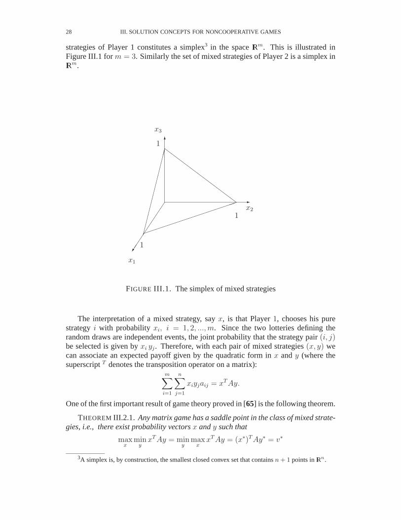
strategies of Player 1 constitutes a simplex3 in the space IRm. This is illustrated inFigure III.1 form = 3. Similarly the set of mixed strategies of Player 2 is a simplex inIRm.
6
x3
À
x1
-x2
³³³³³³³³³³³³³³³
1
1
¤¤¤¤¤¤¤¤¤¤¤¤¤¤ZZ
ZZ
ZZ
ZZ
ZZ
Z
1
FIGURE III.1. The simplex of mixed strategies
The interpretation of a mixed strategy, sayx, is that Player1, chooses his purestrategyi with probability xi, i = 1, 2, ..., m. Since the two lotteries defining therandom draws are independent events, the joint probability that the strategy pair(i, j)be selected is given byxi yj. Therefore, with each pair of mixed strategies(x, y) wecan associate an expected payoff given by the quadratic form inx andy (where thesuperscriptT denotes the transposition operator on a matrix):
m∑i=1
n∑j=1
xiyjaij = xT Ay.
One of the first important result of game theory proved in [65] is the following theorem.
THEOREM III.2.1. Any matrix game has a saddle point in the class of mixed strate-gies, i.e., there exist probability vectorsx andy such that
maxx
miny
xT Ay = miny
maxx
xT Ay = (x∗)T Ay∗ = v∗
3A simplex is, by construction, the smallest closed convex set that containsn + 1 points in IRn.

III.2. MATRIX GAMES 29
wherev∗ is called the value of the game.
We shall not repeat the complex proof given by von Neumann. Instead we willshow that the search for saddle points can be formulated as alinear programmingproblem (LP). A well knownduality propertyin LP implies the saddle point existenceresult.

30 III. SOLUTION CONCEPTS FOR NONCOOPERATIVE GAMES
III.2.4. Algorithms for the computation of saddle-points. Saddle points in mixedstrategies can be obtained as solutions of specific linear programs. It is easy to showthat, for any matrix game, the following two relations hold4:
(III.8) v∗ = maxx
miny
xT Ay = maxx
minj
m∑i=1
xiaij
and
(III.9) z∗ = miny
maxx
xT Ay = miny
maxi
n∑j=1
yjaij
These two relations imply that the value of the matrix game can be obtained by solvingany of the following two linear programs:
(1) Primal problem
max v
subject to
v ≤m∑
i=1
xiaij, j = 1, 2, ..., n
1 =m∑
i=1
xi
xi ≥ 0, i = 1, 2, ...m
(2) Dual problem
min z
subject to
z ≥n∑
j=1
yjaij, i = 1, 2, ..., m
1 =n∑
j=1
yj
yj ≥ 0, j = 1, 2, ...n
The following theorem relates the two programs together.
THEOREM III.2.2. (Von Neumann[65]): Any finite two-person zero-sum matrixgameA has a value.
4Actually this is already a linear programming result. When the vectorx is given, the expressionminy xT Ay, with the simplex constraintsi.e., y ≥ 0 and
∑j yj = 1 defines a linear program. The
solution of that LP can always be found at an extreme point of the admissible set. An extreme pointin the simplex corresponds toyj = 1 and the other components equal to 0. Therefore, since Player 1selects his mixed strategyx expecting the opponent to define his best reply, he can only restrict thesearch for the best reply to the opponent’s set of pure strategies.

III.2. MATRIX GAMES 31
Proof: The valuev∗ of the zero-sum matrix gameA is obtained as the common opti-mal value of the following pair of dual linear programming problems. The respectiveoptimal programs define the saddle-point mixed strategies.
Primal Dualmax v min zsubject to xT A ≥ v1T subject to Ay ≤ z1
xT1 = 1 1T y = 1x ≥ 0 y ≥ 0
where
1 =
1...1...1
denotes a vector of appropriate dimension with all components equal to 1. One needsto solve only one of the programs. The primal and dual solutions give a pair of saddlepoint strategies. QED
REMARK III.2.2. Simplen × n games can be solved more easily (see[47]). Sup-poseA is ann× n matrix game which does not have a saddle point in pure strategies.The players’ unique saddle point mixed strategies and the game value are given by:
(III.10) x =1T AD
1T AD1
(III.11) y =AD1
1T AD1
(III.12) v =detA
1T AD1
whereAD is the adjoint matrix ofA, det A the determinant ofA, and1 the vector ofones as before.
Let us illustrate the usefulness of the above formulae on the following example.
EXAMPLE III.2.3. We want to solve the matrix game[
1 0−1 2
].
The game, obviously, has no saddle point (in pure strategies). The adjointAD is[
2 01 1
]

32 III. SOLUTION CONCEPTS FOR NONCOOPERATIVE GAMES
and1AD = [3 1], AD1T = [2 2], 1AD1T = 4, det A = 2. Hence the bestmixedstrategiesfor the players are:
x =
[3
4,
1
4
], y =
[1
2,
1
2
]
and the value of the play is:
v =1
2
In other words in the long run Player1 is supposed to win.5 if he uses the first row75% of times and the second25% of times. The Player2’s best strategy will be to usethe first and the second column50% of times which ensures him a loss of.5 (only;using other strategies he is supposed to lose more). ¦
III.3. Bimatrix games
III.3.1. Best reply strategies. We shall now extend the theory that we developedfor matrix games to the case of nonzero sum games. Abimatrix gameconvenientlyrepresents a two-person nonzero sum game where each player has a finite set of possi-ble pure strategies. In a bimatrix game there are two players, say Player1 and Player2who havem andn pure strategies to choose from, respectively. Now, if the players se-lect a pair of pure strategies, say(i, j), then Player1 obtains the payoffaij and Player2 obtainsbij, whereaij andbij are some given numbers. The payoffs for the two play-ers corresponding to all possible combinations of pure strategies can be representedby two m × n payoff matricesA andB (from here the name) with entriesaij andbij,respectively. Whenaij + bij = 0, the game is a zero-sum matrix game. Otherwise,the game is nonzero-sum. Asaij and bij are the players’ payoff matrix entires thisconclusion agrees with Definition III.2.1, page 24.
In Remark III.2.1, page 27, in the context of (zero-sum) matrix games, we havenoticed that a pair of saddle point strategies constitute an equilibrium since no playercan improve his payoff by a unilateral strategic change. Each player has thereforechosen the best reply to the strategy of the opponent. We examine whether the conceptof best reply strategies can be also used to define a solution to a bimatrix game.
EXAMPLE III.3.1. Consider the bimatrix game defined by the following matrices[
52 44 4442 46 39
]
and [50 44 4142 49 43
].
Examine whether there are strategy pairs that constitute best reply to each other.

III.3. BIMATRIX GAMES 33
It is often convenient to combine the data contained in two matrices and write it in theform of one matrix whose entries are ordered pairs(aij, bij). In this case one obtains[
(52, 50)∗ (44, 44) (44, 41)(42, 42) (46, 49)∗ (39, 43)
].
Consider the two cells indicated by an asterisks∗. Notice that they correspond tooutcomes resulting from best reply strategies. Indeed, at cell “1,1”, if Player 2 sticksto the first column, Player 1 can only worsen his payoff from 52 to 42, if he moves torow 2. Similarly, if Player 1 plays row 1, Player 2 can gain 44 or 41 only, instead of50, if he abandoned column 1. Similar reasoning can be conducted to prove that thepayoffs at cell “2,2” result from another pair of best reply strategies. ¦
III.3.2. Nash equilibria. We can see from Example III.3.1 that a bimatrix gamecan have many best reply strategy pairs. However there are other examples where nosuch pairs can be found in pure strategies. So, as we have done it with (zero-sum)matrix games, we will expand the strategy sets to include mixed strategies for bimatrixgames. TheNash equilibriumsolution concept for the bimatrix games is defined asfollows.
DEFINITION III.3.1. A pair of mixed strategies(x∗, y∗) is said to be a Nash equi-librium of the bimatrix game if
(1) (x∗)T A(y∗) ≥ xT A(y∗) for every mixed strategyx, and(2) (x∗)T B(y∗) ≥ (x∗)T By for every mixed strategyy.
Notice that this definition simply says that at an equilibrium, no player can improvehis payoff by deviating unilaterally from the equilibrium strategy.
REMARK III.3.1. A Nash equilibrium extends to nonzero sum games the equilib-rium property that was observed for the saddle point solution to a zero sum matrixgame. The big difference with the saddle point concept is that, in a nonzero sum con-text, the equilibrium strategy for a player does not guarantee him that he will receiveat least the equilibrium payoff. Indeed if his opponent does not play “well” i.e., doesnot use the equilibrium strategy, the outcome of a player can be anything. There is noguarantee of the payoff; it is only “hoped” that the other player is rational and in itsown interest will play his best reply strategy.
Another important step in the development of the theory of games has been thefollowing theorem [42]
THEOREM III.3.1. Every finite bimatrix game has at least one Nash equilibrium inmixed strategies.
Proof: A general existence proof for equilibria in concave games, a class of gamesthat include the bimatrix games, based on Kakutani fixed point theorem will be givenin the next section. QED

34 III. SOLUTION CONCEPTS FOR NONCOOPERATIVE GAMES
III.3.3. Shortcommings of the Nash equilibrium concept.
III.3.3.1. Multiple equilibria. As noticed in Example III.3.1 a bimatrix game mayhave several equilibria in pure strategies. There may be additional equilibria in mixedstrategies as well. The nonuniqueness of Nash equilibria for bimatrix games is a se-rious theoretical and practical problem. In Example III.3.1 one equilibrium strictlydominatesthe other equilibriumi.e., gives both players higher payoffs. Thus, it canbe argued that even without any consultations the players will naturally pick the strat-egy pair corresponding to matrix entry(i, j) = (1, 1). However, it is easy to defineexamples where the situation is not so clear.
EXAMPLE III.3.2. Consider the following bimatrix game[
(2, 1)∗ (0, 0)(0, 0) (1, 2)∗
]
It is easy to see that this game5 has two equilibria (in pure strategies), none of whichdominates the other. Moreover, Player1 will obviously prefer the solution(1, 1), whilePlayer2 will rather have(2, 2). It is difficult to decide how this game should be playedif the players are to arrive at their decisions independently of one another.
III.3.3.2. The prisoner’s dilemma.There is a famous example of a bimatrix game,that is used in many contexts to argue that the Nash equilibrium solution is not alwaysa “good” solution to a noncooperative game.
EXAMPLE III.3.3. Suppose that two suspects are held on the suspicion of commit-ting a serious crime. Each of them can be convicted only if the other provides evidenceagainst him, otherwise he will be convicted as guilty of a lesser charge. However, byagreeing to give evidence against the other guy, a suspect can shorten his sentenceby half. Of course, the prisoners are held in separate cells and cannot communicatewith each other. The situation is as described in Table III.1 with the entries giving thelength of the prison sentence for each suspect, in every possible situation. Notice thatin this case, the players are assumed tominimize rather than maximize the outcomeof the play.
Suspect I: Suspect II: refusesagrees to testifyrefuses (2, 2) (10, 1)agrees to testify (1, 10) (5, 5)∗
TABLE III.1. The Prisoner’s Dilemma.
5The above example is classical in game theory and known as the “battle-of-sexes” game. In anAmerican and a rather sexist context, the rows represent the woman’s choices between going to thetheater and the football match while the columns are the man’s choices between the same events. Infact, we can well understand what a mixed-strategy solution means for this example: the couple will behappy if the go to the theater and match in every alternative week.

III.3. BIMATRIX GAMES 35
The unique Nash equilibrium of this game is given by the pair of pure strategies(agree-to-testify, agree-to-testify) with the outcome that both suspects will spend fiveyears in prison. This outcome is strictly dominated by the strategy pair(refuse-to-testify, refuse-to-testify), which however is not an equilibrium and thus is not a realisticsolution of the problem when the players cannot make binding agreements. ¦
The above example shows that Nash equilibria could result in outcomes being veryfar from efficient.
III.3.4. Algorithms for the computation of Nash equilibria in bimatrix games.Linear programming is closely associated with the characterization and computationof saddle points in matrix games. For bimatrix games one has to rely on algorithmssolving eitherquadratic programmingor complementarityproblems, which we definebelow. There are also a few algorithms (see [3], [47]) which permit us to find anequilibrium of simple bimatrix games. We will show one for a2 × 2 bimatrix gameand then introduce the quadratic programming [38] and complementarity problem [34]formulations.
III.3.4.1. Equilibrium computation in a2 × 2 bimatrix game.For a simple2 ×2 bimatrix game one can easily find a mixed strategy equilibrium as shown in thefollowing example.
EXAMPLE III.3.4. Consider the game with payoff matrix given below.
[(1, 0) (0, 1)(1
2, 1
3) (1, 0)
]
Compute a mixed strategy equilibrium.
First, notice that this game has no pure strategy equilibrium.
Assume Player2 chooses his equilibrium strategyy (i.e.,100y% of times use firstcolumn,100(1 − y)% times use second column) in such a way that Player1 (in equi-librium) will get as much payoff using first row as using second rowi.e.,
y + 0(1− y) =1
2y + 1(1− y).
This is true fory∗ = 23.
Symmetrically, assume Player1 is using a strategyx (i.e.,100x% of times use firstrow, 100(1 − y)% times use second row) such that Player2 will get as much payoffusing first column as using second columni.e.,
0x +1
3(1− x) = 1x + 0(1− x).

36 III. SOLUTION CONCEPTS FOR NONCOOPERATIVE GAMES
This is true forx∗ = 14. The players’ payoffs will be, respectively,(2
3) and(1
4).
Then the pair of mixed strategies
(x∗, 1− x∗), (y∗, 1− y∗)
is an equilibrium in mixed strategies. ¦
III.3.4.2. Links between quadratic programming and Nash equilibria in bimatrixgames.Mangasarian and Stone (1964) have proved the following result that links qua-dratic programming with the search of equilibria in bimatrix games. Consider a bima-trix game(A, B). We associate with it the quadratic program
max [xT Ay + xT By − v1 − v2](III.13)
s.t.
Ay ≤ v11m(III.14)
BT x ≤ v21n(III.15)
x, y ≥ 0(III.16)
xT1m = 1(III.17)
yT1n = 1(III.18)
v1, v2, ∈ IR.(III.19)
LEMMA III.3.1. The following two assertions are equivalent
(i): (x, y, v1, v2) is a solution to the quadratic programming problem (III.13)-(III.19)
(ii): (x, y) is an equilibrium for the bimatrix game.
Proof: From the constraints it follows thatxT Ay ≤ v1 andxT By ≤ v2 for any feasible(x, y, v1, v2). Hence the maximum of the program is at most 0. Assume that(x, y) isan equilibrium for the bimatrix game. Then the quadruple
(x, y, v1 = xT Ay, v2 = xT By)
is feasiblei.e., satisfies (III.14)-(III.19); moreover, it gives a value 0 to the objectivefunction (III.13). Hence the equilibrium defines a solution to the quadratic program-ming problem (III.13)-(III.19).
Conversely, let(x∗, y∗, v1∗, v
2∗) be a solution to the quadratic programming problem
(III.13)- (III.19). We know that an equilibrium exists for a bimatrix game (Nash theo-rem). We know that this equilibrium is a solution to the quadratic programming prob-lem (III.13)-(III.19) with optimal value 0. Hence the optimal program(x∗, y∗, v1
∗, v2∗)
must also give a value 0 to the objective function and thus be such that
xT∗Ay∗ + xT
∗By∗ = v1∗ + v2
∗.(III.20)

III.3. BIMATRIX GAMES 37
For anyx ≥ 0 andy ≥ 0 such thatxT1m = 1 andyT1n = 1 we have, by (III.17) and(III.18)
xT Ay∗ ≤ v1∗
xT∗By ≤ v2
∗ .
In particular we must have
xT∗Ay∗ ≤ v1
∗xT∗By∗ ≤ v2
∗
These two conditions with (III.20) imply
xT∗Ay∗ = v1
∗xT∗By∗ = v2
∗ .
Therefore we can conclude that For anyx ≥ 0 andy ≥ 0 such thatxT1m = 1 andyT1n = 1 we have, by (III.17) and (III.18)
xT Ay∗ ≤ xT∗Ay∗
xT∗By ≤ xT
∗By∗
and hence,(x∗, y∗) is a Nash equilibrium for the bimatrix game. QED
III.3.4.3. A complementarity problem formulation.We have seen that the searchfor equilibria could be done through solving a quadratic programming problem. Herewe show that the solution of a bimatrix game can also be obtained as the solution of acomplementarity problem.
There is no loss in generality if we assume that the payoff matrices arem× n andhave only positive entries (A > 0 andB > 0). This is not restrictive, since VNMutilities are defined up to an increasing affine transformation. A strategy for Player 1is defined as a vectorx ∈ IRm that satisfies
x ≥ 0(III.21)
xT1m = 1(III.22)
and similarly for Player 2
y ≥ 0(III.23)
yT1n = 1.(III.24)
It is easily shown that the pair(x∗, y∗) satisfying (III.21)-(III.24) is an equilibrium iff
(III.25)(x∗
TAy∗)1m ≥ A y∗ (A > 0)
(x∗TB y∗)1n ≥ BT x∗ (B > 0)
i.e., if the equilibrium condition is satisfied for pure strategy alternatives only.

38 III. SOLUTION CONCEPTS FOR NONCOOPERATIVE GAMES
Consider the following set of constraints withv1 ∈ IR andv2 ∈ IR
(III.26)v11m ≥ Ay∗
v21n ≥ BT x∗and
x∗T(Ay∗ − v11m) = 0
y∗T(BT x∗ − v21n) = 0
.
The relations on the right are calledcomplementarity constraints. For mixed strategies(x∗, y∗) satisfying (III.21)-(III.24), they simplify tox∗
TAy∗ = v1, x∗
TB y∗ = v2. This
shows that the above system (III.26) of constraints is equivalent to the system (III.25).
Define s1 = x/v2, s2 = y/v1 and introduce the slack variablesu1 andu2, thesystem of constraints (III.21)-(III.24) and (III.26) can be rewritten(
u1
u2
)=
(1m
1n
)−
(0 A
BT 0
) (s1
s2
)(III.27)
0 =
(u1
u2
)T (s1
s2
)(III.28)
0 ≤(
u1
u2
)T
(III.29)
0 ≤(
s1
s2
).(III.30)
Introducing four obvious new variables permits us to rewrite (III.27)- (III.30) in thegeneric formulation
u = q + Ms(III.31)
0 = uT s(III.32)
u ≥ 0(III.33)
s ≥ 0,(III.34)
of a so-called acomplementarity problem.
A pivoting algorithm ([34], [35]) has been proposedto solve such problems. Thisalgorithm applies also toquadratic programming, so this confirms that the solution ofa bimatrix game is of the same level of difficulty as solving a quadratic programmingproblem.
REMARK III.3.2. Once we obtainx and y, solution to (III.27)-(III.30) we shallhave to reconstruct the strategies through the formulae
x = s1/(sT1 1m)(III.35)
y = s2/(sT2 1n).(III.36)
III.4. Concave m-person games
The nonuniqueness of equilibria in bimatrix games and a fortiori inm-player ma-trix games poses a delicate problem. If there are many equilibria, in a situation whereone assumes that the players cannot communicate or enter into preplay negotiations,

III.4. CONCAVE m-PERSON GAMES 39
how will a given player choose among the different strategies corresponding to the dif-ferent equilibrium candidates? In single agent optimization theory we know that strictconcavity of the (maximized) objective function and compactness and convexity of theconstraint set lead to existence and uniqueness of the solution. The following questionthus arises
Can we generalize the mathematical programming approach to asituation where the optimization criterion is a Nash-Cournot equi-librium? can we then give sufficient conditions for existence anduniqueness of an equilibrium solution?
The answer has been given by Rosen in a seminal paper [54] dealing withconcavem-person game.
A concavem-person gameis described in terms of individual strategies repre-sented by vectors in compact subsets of Euclidian spaces (IRmj for Playerj) and bypayoffs represented, for each player, by a continuous functions which is concave w.r.t.his own strategic variable. This is a generalization of the concept of mixed strategies,introduced in previous sections. Indeed, in a matrix or a bimatrix game the mixedstrategies of a player are represented as elements of asimplex i.e.,a compact con-vex set, and the payoffs arebilinear or multilinear forms of the strategies, hence, foreach player the payoff is concave w.r.t. his own strategic variable. This structure isthus generalized in two ways: (i) the strategies can be vectors constrained to be in amore general compact convex set and (ii) the payoffs are represented by more generalcontinuous-concave functions.
Let us thus introduce the following game in strategic form
• Each playerj ∈ M = {1, . . . , m} controls the actionuj ∈ Uj whereUj isa compact convex subset of IRmj , whith mj a given integer. Playerj receivesa payoffψj(u1, . . . , uj, . . . , um) that depends on the actions chosen by all theplayers. One assumes that the reward functionψj : U1×· · ·×Uj, · · ·×Um 7→IR is continuous in eachui and concave inuj.
• A coupled constraintis defined as a proper subsetU of U1×· · ·×Uj ×· · ·×Um. The constraint is that the joint actionu = (u1, . . . , um) must be inU .
DEFINITION III.4.1. An equilibrium , under the coupled constraintU is defined asa decisionm-tuple(u∗1, . . . , u
∗j , . . . , u
∗m) ∈ U such that for each playerj ∈ M
ψj(u∗1, . . . , u
∗j , . . . , u
∗m) ≥ ψj(u
∗1, . . . , uj, . . . , u
∗m)(III.37)
for all uj ∈ Uj s.t. (u∗1, . . . , uj, . . . , u∗m) ∈ U .(III.38)
REMARK III.4.1. The consideration of a coupled constraint is a new feature. Noweach player’s strategy space may depend on the strategy of the other players. Thismay look awkward in the context of nonocooperative games where the players cannotenter into communication or cannot coordinate their actions. However the concept is

40 III. SOLUTION CONCEPTS FOR NONCOOPERATIVE GAMES
mathematically well defined. We shall see later on that it fits very well some interestingaspects of environmental management. One can think for example of a global emissionconstraint that is imposed on a finite set of firms that are competing on the same market.This environmental example will be further developed in forthcoming chapters.
III.4.1. Existence of coupled equilibria.
DEFINITION III.4.2. A coupled equilibrium is a vectoru∗ such that
(III.39) ψj(u∗) = max
uj
{ψj(u∗1, . . . , uj, . . . , u
∗m)|(u∗1, . . . , uj, . . . , u
∗m) ∈ U}.
At such a point no player can improve his payoff by a unilateral change in his strategywhich keeps the combined vector inU .
Let us first show that an equilibrium is actually defined through afixed pointcondi-tion. For that purpose we introduce a so-calledglobal reaction functionθ : U×U 7→ IRdefined by
(III.40) θ(u,v, r) =m∑
j=1
rjψj(u1, . . . , vj, . . . , um),
where the coefficientsrj > 0, j = 1, . . . ,m are arbitrary given positive weights. Theprecise role of this weighting scheme will be explained later. For the moment wecould take as wellrj ≡ 1. Notice that, even ifu andv are inU , the combined vectors(u1, . . . , vj, . . . , um) are element of a larger set inU1 × . . . × Um. This function iscontinuous inu and concave inv for every fixedu. We call it areaction functionsincethe vectorv can be interpreted as composed of the reactions of the different players tothe given vectoru. This function is helpful as shown in the following result.
LEMMA III.4.1. Letu∗ ∈ U be such that
(III.41) θ(u∗,u∗, r) = maxu∈U
θ(u∗,u, r).
Thenu∗ is a coupled equilibrium.
Proof: Assumeu∗ satisfies (III.41) but is not a coupled equilibriumi.e., does notsatisfy (III.39). Then, for one player, say`, there would exist a vector
u = (u∗1, . . . , u`, . . . , u∗m) ∈ U
such thatψ`(u
∗1, . . . , u`, . . . , u
∗m) > ψ`(u
∗).Then we shall also haveθ(u∗, u) > θ(u∗,u∗) which is a contradiction to (III.41).QED
This result has two important consequences.
(1) It shows that proving the existence of an equilibrium reduces to proving thata fixed pointexists for an appropriately definedreaction mapping(u∗ is thebest reply tou∗ in (III.41));

III.4. CONCAVE m-PERSON GAMES 41
(2) it associates with an equilibrium animplicit maximization problem, definedin (III.41). We say that this problem isimplicit since it is defined in terms ofthe very solutionu∗ that it characterizes.
To make more precise the fixed point argument we introduce acoupled reaction map-ping.
DEFINITION III.4.3. The point to set mapping
(III.42) Γ(u, r) = {v|θ(u,v, r) = maxw∈U
θ(u,w, r)}.is called the coupled reaction mapping associated with the positive weightingr. Afixed point ofΓ(·, r) is a vectoru∗ such thatu∗ ∈ Γ(u∗, r).
By Lemma III.4.1 a fixed point ofΓ(·, r) is a coupled equilibrium.
THEOREM III.4.1. For any positive weightingr there exists a fixed point ofΓ(·, r)i.e., a pointu∗ s.t.u∗ ∈ Γ(u∗, r). Hence a coupled equilibrium exists.
Proof: The proof is based on the Kakutani fixed-point theorem that is given in theAppendix of section III.7. One is required to show that the point to set mapping isupper semicontinuous. This is an easy consequence of the concavity of the game andcompactness of all constraint setsUj, j = 1, . . . ,m andU . QED
REMARK III.4.2. This existence theorem is very close, in spirit, to the theorem ofNash. It uses a fixed-point result which is “topological” and not “constructive” i.e.,it does not provide a computational method. However, the definition of anormalisedequilibrium introduced by Rosen establishes a link between mathematical program-ming and concave games with coupled constraints.
III.4.2. Normalized equilibria.
III.4.2.1. Kuhn-Tucker multipliers.Suppose that the coupled constraint (III.39)can be defined by a set of inequalities
(III.43) hk(u) ≥ 0, k = 1, . . . , p
wherehk : U1 × · · · × Um → IR, k = 1, . . . , p, are given concave functions. Letus further assume that the payoff functionsψj(·) as well as the constraint functionshk(·) are continuously differentiable and satisfy the constraint qualification conditionsso that Kuhn-Tucker multipliers exist for each of the implicit single agent optimizationproblems defined below.
Assume all players other than Playerj use their strategyu∗i , i ∈ M , i 6= j. Thenthe equilibrium conditions (III.37)-(III.39) define a single agent optimization problemwith concave objective function and convex compact admissible set. As usual, wedenote[u∗−j, uj] the decision vector where all playersi other thanj play u∗i while
42 III. SOLUTION CONCEPTS FOR NONCOOPERATIVE GAMES
Playerj usesuj. Under the assumed constraint qualification assumption there exists avector of Kuhn-Tucker multipliersλj = (λjk)k=1,...,p such that the Lagrangean
(III.44) Lj([u∗−j, uj], λj) = ψj([u
∗−j, uj]) +∑
k=1...p
λjkhk([u∗−j, uj])
verifies, at the optimum
0 =∂
∂uj
Lj([u∗−j, u∗j ], λj)(III.45)
0 ≤ λj(III.46)
0 = λjkhk([u∗−j, u∗j ]) k = 1, . . . , p.(III.47)
DEFINITION III.4.4. We say that the equilibrium is normalized if the different mul-tipliers λj for j ∈ M are colinear with a common vectorλ0, namely
(III.48) λj =1
rj
λ0
where the coefficientsrj > 0, j = 1, . . . , m are weights given to the players.
Actually, this common multiplierλ0 is associated with the implicit mathematicalprogramming problem
(III.49) maxu∈U
θ(u∗,u, r)
to which we associate the Lagrangean
(III.50) L0(u, λ0) =∑j∈M
rjψj([u∗−j, uj]) +
∑
k=1...p
λ0khk(u).
and the first order necessary conditions
0 =∂
∂uj
{rjψj(u∗) +
∑
k=1,...,p
λ0khk(u∗)}, j ∈ M(III.51)
0 ≤ λ0(III.52)
0 = λ0khk(u∗) k = 1, . . . , p.(III.53)
III.4.2.2. An economic interpretation.The multiplier, in a mathematical program-ming framework, can be interpreted as a marginal cost associated with the right-handside of the constraint. More precisely it indicates the sensitivity of the optimum solu-tion to marginal changes in this right-hand-side. The multiplier permits also apricedecentralizationin the sense that, through an ad-hoc pricing mechanism the optimiz-ing agent is induced to satisfy the constraints. In a normalized equilibrium, the shadowcost interpretation is not so apparent; however, theprice decomposition principleisstill valid. Once the common multiplier has been defined, with the associated weight-ing rj > 0, j = 1, . . . , m, the coupled constraint will be satisfied by equilibrium

III.4. CONCAVE m-PERSON GAMES 43
seeking players, when they use as payoffs the Lagrangeans
Lj([u∗−j, uj], λj) = ψj([u
∗−j, uj]) +1
rj
∑
k=1...p
λ0khk([u∗−j, uj]),
j = 1, . . . ,m.(III.54)
The common multiplier permits then an “implicit pricing” of the common constraintso that it remains compatible with the equilibrium structure. Indeed, this result to beuseful necessitates uniqueness of the normalized equilibrium associated with a givenweightingrj > 0, j = 1, . . . , m. In a mathematical programming framework, unique-ness of an optimum results from strict concavity of the objective function to be max-imized. In a game structure, uniqueness of the equilibrium will result from a morestringent strict concavity requirement, called by Rosenstrict diagonal concavity.
III.4.3. Uniqueness of equilibrium. Let us consider the so-calledpseudo-gradientdefined as the vector
(III.55) g(u, r) =
r1∂
∂u1ψ1(u)
r2∂
∂u2ψ2(u)...
rm∂
∂umψm(u)
We notice that this expression is composed of the partial gradients of the differentpayoffs with respect to the decision variables of the corresponding player. We alsoconsider the function
(III.56) σ(u, r) =m∑
j=1
rjψj(u)
DEFINITION III.4.5. The functionσ(u, r) is diagonally strictly concaveonU if,for everyu1 andu2 in U , the following holds
(III.57) (u2 − u1)T g(u1, r) + (u1 − u2)T g(u2, r) > 0.
A sufficient condition thatσ(u, r) bediagonally strictly concaveis that the sym-metric matrix[G(u, r)+G(u, r)T ] be negative definite for anyu1 in U , whereG(u, r)is the Jacobian ofg(u0, r) with respect tou.
THEOREM III.4.2. If σ(u, r) is diagonally strictly concaveon the convex setU ,with the assumptions insuring existence of K.T. multipliers, then for everyr > 0 thereexists a unique normalized equilibrium
Proof.We sketch below the proof given by Rosen [54]. Assume that for somer > 0 we have two equilibriau1 andu2. Then we must have
h(u1) ≥ 0(III.58)
h(u2) ≥ 0(III.59)

44 III. SOLUTION CONCEPTS FOR NONCOOPERATIVE GAMES
and there exist multipliersλ1 ≥ 0, λ2 ≥ 0, such that
λ1T
h(u1) = 0(III.60)
λ2T
h(u2) = 0(III.61)
and for which the following holds true for each playerj ∈ M
rj∇ujψj(u
1) + λ1T∇ujh(u1) = 0(III.62)
rj∇ujψj(u
2) + λ2T∇ujh(u2) = 0.(III.63)
We multiply (III.62) by (u2 − u1)T and (III.63) by(u1 − u2)T and we sum togetherto obtain an expressionβ + γ = 0, where, due to the concavity of thehk and theconditions (III.58)-(III.61)
γ =∑j∈M
p∑
k=1
{λ1k(u
2 − u1)T∇ujhk(u
1) + λ2k(u
1 − u2)T∇ujhk(u
2)}
≥∑j∈M
{λ1T
[h(u2)− h(u1)] + λ2T
[h(u1)− h(u2)]}
=∑j∈M
{λ1T
h(u2) + λ2T
h(u1)} ≥ 0,(III.64)
and
β =∑j∈M
rj[(u2 − u1)T∇uj
ψj(u1) + (u1 − u2)T∇uj
ψj(u2)].(III.65)
Sinceσ(u, r) is diagonally strictly concave we haveβ > 0 which contradictsβ+γ = 0.QED
III.4.4. A numerical technique. The diagonal strict concavity property that yieldedthe uniqueness result of theorem III.4.2 also provides an interesting extension of thegradient method for the computation of the equilibrium. The basic idea is to ”project”,at each step, the pseudo gradientg(u, r) on the constraint setU = {u : h(u) ≥ 0} (letus callg(u`, r) this projection) and to proceed through the usual steepest ascent step
u`+1 = u` + τ `g(u`, r).
Rosen shows that, at each step` the step sizeτ ` > 0 can be chosen small enough forhaving a reduction of the norm of the projected gradient. This yields convergence ofthe procedure toward the unique equilibrium.
III.4.5. A variational inequality formulation.
THEOREM III.4.3. Under assumptions IV.1.1 the vectorq∗ = (q∗1, . . . , q∗m) is a
Nash-Cournot equilibrium if and only if it satisfies the followingvariational inequality
(III.66) (q− q∗)T g(q∗) ≤ 0,
whereg(q∗) is the pseudo-gradient atq∗ with weighting1.

III.5. CORRELATED EQUILIBRIA 45
Proof: Apply first order necessary and sufficient optimality conditions for each playerand aggregate to obtain (III.66). QED
REMARK III.4.3. The diagonal strict concavity assumption is then equivalent tothe property ofstrong monotonicityof the operatorg(q∗) in the parlance of varia-tional inequality theory.
III.5. Correlated equilibria
Aumann, [2], has proposed a mechanism that permits the players to enter intopreplay arrangements so that their strategy choices could be correlated, instead of beingindependently chosen, while keeping an equilibrium property. He called this type ofsolutioncorrelated equilibrium.
III.5.1. Example of a game with correlated equlibria.
EXAMPLE III.5.1. This example has been initially proposed by Aumann[2]. Con-sider a simple bimatrix game defined as follows
c1 c2
r1 5, 1 0, 0r2 4, 4 1, 5
This game has two pure strategy equilibria(r1, c1) and (r2, c2) and a mixed strategyequilibrium where each player puts the same probality 0.5 on each possible pure strat-egy. The respective outcomes are shown in Table III.2 Now, if the players agree to play
(r1, c1) : 5,1(r2, c2) : 1,5
(0.5− 0.5, 0.5− 0.5) : 2.5,2.5TABLE III.2. Outcomes of the three equilibria
by jointly observing a “coin flip” and playing(r1, c1) if the result is “head”,(r2, c2) ifit is “tail” then they expect the outcome3, 3 which is a convex combination of the twopure equilibrium outcomes.
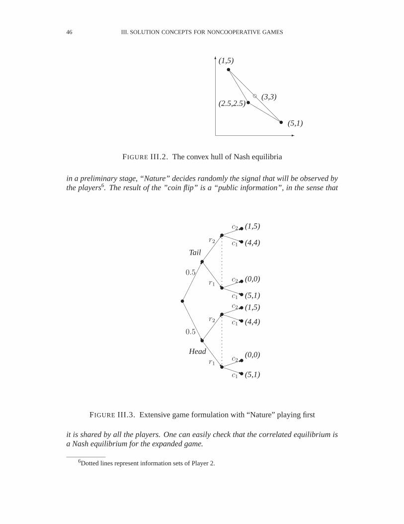
By deciding to have a coin flip deciding on the equilibrium to play, a new type ofequilibrium has been introduced that yields an outcome located in the convex hull ofthe set of Nash equilibrium outcomes of the bimatrix game. In Figure III.2 we haverepresented these different outcomes. The three full circles represent the three Nashequilibrium outcomes. The triangle defined by these three points is the convex hull ofthe Nash equilibrium outcomes. The empty circle represents the outcome obtained byagreeing to play according to the coin flip mechanism.
It is easy to see that this way to play the game defines an equilibrium for the exten-sive game shown in Figure III.3. This is an expanded version of the initial game where,
46 III. SOLUTION CONCEPTS FOR NONCOOPERATIVE GAMES
-
6t
t
td (3,3)
(2.5,2.5)
(1,5)
(5,1)@@
@@
@@
@@
TT
TT
T
bb
bb
b
FIGURE III.2. The convex hull of Nash equilibria
in a preliminary stage, “Nature” decides randomly the signal that will be observed bythe players6. The result of the ”coin flip” is a “public information”, in the sense that
t¢¢¢¢¢¢
AAAAAAUt
Head
Tailt
¶¶
¶7
SS
SSw
¶¶
¶¶7
SS
SSwt
t
t
t
ppppppppppppppppp
ppppppppppppppppp
³³³1PPPq
³³³1PPPq
³³³1PPPq
³³³1PPPq
c1
c1
c1
c1
c2
c2
c2
c2
r1
r1
r2
r2
tt
tt
tt
tt
(5,1)
(0,0)
(4,4)
(1,5)
(5,1)
(0,0)
(4,4)
(1,5)
0.5
0.5
FIGURE III.3. Extensive game formulation with “Nature” playing first
it is shared by all the players. One can easily check that the correlated equilibrium isa Nash equilibrium for the expanded game.
6Dotted lines represent information sets of Player 2.

III.5. CORRELATED EQUILIBRIA 47
c1 c2
r113
0r2
13
13
FIGURE III.4. Probabilities of signals
We now push the example one step further by assuming that the players agree toplay according to the following mechanism: A random device selects one cell in thegame matrix with the probabilities shown in Figure III.4.
When a cell is selected, then each player is told to play the corresponding purestrategy. The trick is that a player is told what to play but is not told what the rec-ommendation to the other player is. The information received by each player is not“public” anymore. More precisely, the three possible signals are(r1, c1), (r2, c1),(r2, c2). When Player 1 receives the signal “playr2” he knows that with a probability12
the other player has been told “playc1” and with a probability 12
the other player hasbeen told “playc2”. When Player 1 receives the signal “playr1” he knows that witha probability1 the other player has been told “playc1”. Consider now what Player 1can do, if he assumes that the other player plays according to the recommendation. IfPlayer 1 has been told “playr2” and if he plays so he expects
1
2× 4 +
1
2× 1 = 2.5;
if he playsr1 instead he expects1
2× 5 +
1
2× 0 = 2.5
so he cannot improve his expected reward. If Player 1 has been told “playr1” andif he plays so he expects5, whereas if he playsr2 he expects4. So, for Player 1,obeying to the recommendation is the best reply to Player 2 behavior when he himselfplays according to the suggestion of the signalling scheme. Now we can repeat theverification for Player 2. If he has been told “playc1” he expects
1
2× 1 +
1
2× 4 = 2.5;
if he playsc2 instead he expects1
2× 0 +
1
2× 5 = 2.5
so he cannot improve. If he has been told “playc2” he expects5 whereas if he playsc1 instead he expects4 so he is better off with the suggested play. So we have checkedthat an equilibrium property holds for this way of playing the game. All in all, eachplayer expects
1
3× 5 +
1
3× 1 +
1
3× 4 = 3 +
1
3from a game played in this way. This is illustrated in Figure III.5 where the black spadeshows the expected outcome of this mode of play. Auman called it a ”correlated equi-librium”. Indeed we can now mix these equilibria and still keep the correlated equi-

48 III. SOLUTION CONCEPTS FOR NONCOOPERATIVE GAMES
-
6t
t
td (3,3)
(2.5,2.5)
(1,5)
(5,1)@@
@@
@@
@@
TT
TT
T
bb
bb
b
(3.33,3.33)♠········
····
············
FIGURE III.5. The dominating correlated equilibrium
librium property, as indicated by the doted line on Figure III.5; also we can constructan expanded game in extensive form for which the correlated equilibrium constructedas above defines a Nash equilibrium (see Exercise 3.6).
In the above example we have seen that, by expanding the game via the adjunction ofa first stage where “Nature” plays and gives information to the players, a new classof equilibria can be reached that dominate, in the outcome space, some of the originalNash-equilibria. If the random device gives an information which is common to allplayers, then it permits a mixing of the different pure strategy Nash equilibria and theoutcome is in the convex hull of the Nash equilibrium outcomes. If the random devicegives an information which may be different from one player to the other, then thecorrelated equilibrium can have an outcome which lies outside of the convex hull ofNash equilibrium outcomes.
III.5.2. A general definition of correlated equilibria. Let us give a general defi-nition of a correlated equilibrium in anm-player normal form game. We shall actuallygive two definitions. The first one describes the construct of anexpanded gamewitha random device distributing some pre-play information to the players. The seconddefinition which is valid form-matrix games is much simpler although equivalent.
III.5.2.1. Nash equilibrium in an expanded game.Assume that a game is de-scribed in normal form, withm playersj = 1, . . . , m, their respective strategy setsΓj and payoffsVj(γ1, . . . , γj, . . . , γm). This will be called theoriginal normal formgame.
Assume the players may enter into a phase ofpre-play communicationduringwhich they design acorrelation devicethat will provide randomly a signal calledpro-posed mode of play. Let E = {1, 2, . . . , L} be the finite set of the possible modes ofplay. The correlation device will propose with probabilityλ(`) the mode of play .The device will then give the different players some information about theproposedmode of play. More precisely, letHj be a class of subsets ofE, called theinformation

III.6. BAYESIAN EQUILIBRIUM WITH INCOMPLETE INFORMATION 49
structureof Playerj. Playerj, when the mode of playhas been selected, receives aninformation denotedhj(`) ∈ Hj. Now, we associate with each playerj ameta strategydenotedγj : Hj → Γj that determines a strategy for the original normal form game,on the basis of the information received. All this construct, is summarized by the data(E, {λ(`)}`∈E, {hj(`) ∈ Hj}j∈M,`∈E, {γj : Hj → Γj}j∈M) that defines anexpandedgame.
DEFINITION III.5.1. The data(E, {λ(`)}`∈E, {hj(`) ∈ Hj}j∈M,`∈E, {γ∗j : Hj →Γj}j∈M) defines a correlated equilibrium of the original normal form game if it is aNash equilibrium for the expanded game i.e., if no player can improve his expectedpayoff by changing unilaterally his meta strategy i.e., by playingγj(hj(`)) instead ofγ∗j (hj(`)) when he receives the signalhj(`) ∈ Hj.(III.67)∑
`∈E
λ(`)Vj([γ∗j (hj(`)), γ
∗M−j(hM−j(`))] ≥
∑
`∈E
λ(`)Vj([γj(hj(`)), γ∗M−j(hM−j(`))].
III.5.2.2. An equivalent definition form-matrix games.In the case of anm-matrixgame, the definition given above can be replaced with the following one, which ismuch simpler
DEFINITION III.5.2. A correlated equilibrium is a probability distributionπ(s)over the set of pure strategiesS = S1 × S2 · · · × Sm such that, for every Playerj andany mappingδj : Sj → Sj the following holds
(III.68)∑s∈S
π(s)Vj([sj, sM−j]) ≥∑s∈S
π(s)Vj([δ(sj), sM−j]).
III.6. Bayesian equilibrium with incomplete information
Up to now we have considered only games where each player knows everythingconcerning the rules, the players types (i.e., their payoff functions, their strategy sets)etc. .. We were dealing withgames of complete information. In this section we lookat a particular class ofgames with incomplete informationand we explore the class ofso-calledBayesian equilibria.
III.6.1. Example of a game with unknown type for a player. In a game of in-complete information, some players do not know exactly what are the characteristicsof other players. For example, in a two-player game, Player 2 may not know exactlywhat the payoff function of Player 1 is.
EXAMPLE III.6.1. Consider the case where Player 1 could be of two types, calledθ1 andθ2 respectively. We define below two matrix games, corresponding to the twopossible types respectively:
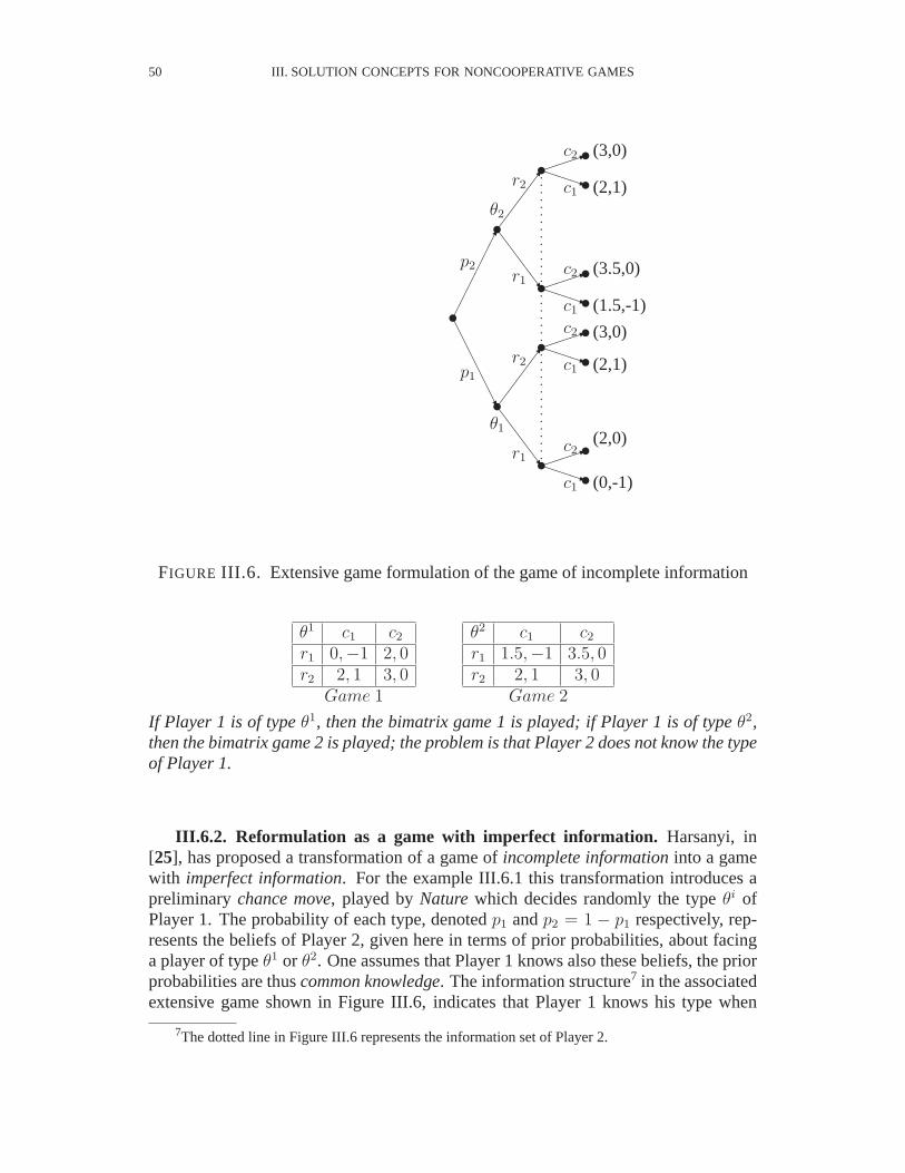
50 III. SOLUTION CONCEPTS FOR NONCOOPERATIVE GAMES
t¢¢¢¢¢¢
AAAAAAUtθ1
tθ2
¶¶
¶7
SS
SSw
¶¶
¶¶7
SS
SSwt
t
t
t
³³³1PPPq
³³³1PPPq
³³³1PPPq
³³³1PPPq
tt
tt
tt
tt
pppppppppppppppppppppppppppppppppppppppp
(0,-1)
(2,0)
(2,1)
(3,0)
(1.5,-1)
(3.5,0)
(2,1)
(3,0)
c1
c1
c1
c1
c2
c2
c2
c2
r1
r1
r2
r2
p1
p2
FIGURE III.6. Extensive game formulation of the game of incomplete information
θ1 c1 c2
r1 0,−1 2, 0r2 2, 1 3, 0
θ2 c1 c2
r1 1.5,−1 3.5, 0r2 2, 1 3, 0
Game 1 Game 2
If Player 1 is of typeθ1, then the bimatrix game 1 is played; if Player 1 is of typeθ2,then the bimatrix game 2 is played; the problem is that Player 2 does not know the typeof Player 1.
III.6.2. Reformulation as a game with imperfect information. Harsanyi, in[25], has proposed a transformation of a game ofincomplete informationinto a gamewith imperfect information. For the example III.6.1 this transformation introduces apreliminarychance move, played byNaturewhich decides randomly the typeθi ofPlayer 1. The probability of each type, denotedp1 andp2 = 1 − p1 respectively, rep-resents the beliefs of Player 2, given here in terms of prior probabilities, about facinga player of typeθ1 or θ2. One assumes that Player 1 knows also these beliefs, the priorprobabilities are thuscommon knowledge. The information structure7 in the associatedextensive game shown in Figure III.6, indicates that Player 1 knows his type when
7The dotted line in Figure III.6 represents the information set of Player 2.

III.6. BAYESIAN EQUILIBRIUM WITH INCOMPLETE INFORMATION 51
deciding, whereas Player 2 does not observe the type neither, indeed in that game ofsimultaneous moves, the action chosen by Player 1. Callxi (respectively1 − xi) theprobability of choosingr1 (respectivelyr2) by Player 1 when he implements a mixedstrategy, knowing that he is of typeθi. Call y (respectively1 − y) the probability ofchoosingc1 (respectivelyc2) by Player 2 when he implements a mixed strategy.
We can define the optimal response of Player 1 to the mixed strategy(y, 1− y) ofPlayer 2 by solving8
maxi=1,2
aθ1
i1 y + aθ1
i2 (1− y)
if the type isθ1,maxi=1,2
aθ2
i1 y + aθ2
i2 (1− y)
if the type isθ2.
We can define the optimal response of Player 2 to the pair of mixed strategy(xi, 1−xi), i = 1, 2 of Player 1 by solving
maxj=1,2
p1(x1bθ1
1j + (1− x1)bθ1
2j) + p2(x2bθ2
1j + (1− x2)bθ2
2j).
Let us rewrite these conditions with the data of the game illustrated in Figure III.6.First consider the reaction function of Player 1
θ1 ⇒ max{0y + 2(1− y), 2y + 3(1− y)}θ2 ⇒ max{1.5y + 3.5(1− y), 2y + 3(1− y)}.
We draw in Figure III.7 the lines corresponding to these comparisons between twolinear functions. We observe that, if Player 1’s type isθ1, he will always chooser2,
-
6
HHHHHHHHHH
XXXXXXXXXX
pppppppppppppppppppp
p p p p p p p p p p p p p p p p p p p pp p p p p p p p p p p p p p p p p p p p
0 1
y
r1
r2
θ1
2
3
-
6
HHHHHHHHHH
XXXXXXXXXX
pppppppppppppppppppp
p p p p p p p p p p p p p p p p p p p p
p p p p p p p p p p p p p p p p p p p p
p p p p p p p p p p p p p p p p p p p p
pppppppppppppppppppp
0 10.5
y
θ2
3.53
21.5
r1
r2
FIGURE III.7. Optimal reaction of Player 1 to Player 2 mixed strategy(y, 1− y)
8We callaθ`
ij andbθ`
ij the payoffs of Player 1 and Player 2 respectively when the type isθ`.
52 III. SOLUTION CONCEPTS FOR NONCOOPERATIVE GAMES
whatevery, whereas, if his type isθ2 he will chooser1 if y is mall enough and switchto r2 wheny > 0.5. Fory = 0.5, the best reply of Player 1 could be any mixed strategy(x, 1− x).
Consider now the optimal reply of Player 2. We know that Player 1, if he is of typeθ1, always chooses actionr2 i.e.,x1 = 0. So the best reply conditions for Player 2 canbe written as follows
max{(p1(1) + (1− p1)(x2(−1) + (1− x2)1)), (p1(0) + (1− p1)(x2(0) + (1− x2)0))}which boils down to
max{(1− 2(1− p1)x2), 0)}.We conclude that Player 2 chooses actionc1 if x2 < 1
2(1−p1), actionc2 if x2 > 1
2(1−p1)
and any mixed action withy ∈ [0, 1] if x2 = 12(1−p1)
. We conclude easily from theseobservations that the equilibria of this game are characterized as follows:
x1 ≡ 0if p1 ≤ 0.5 x2 = 0, y = 1 or x2 = 1, y = 0 or x2 = 1
2(1−p1), y = 0.5
if p1 > 0.5 x2 = 0, y = 1.
III.6.3. A general definition of Bayesian equilibria. We can generalize the anal-ysis performed on the previous example and introduce the following definitions. LetM be a set ofm players. Each playerj ∈ M may be of different possible types. LetΘj be the finite set of types for Playerj. Whatever his type, Payerj has the same setof pure strategiesSj. If θ = (θ1, . . . .θm) ∈ Θ = Θ1 × · · · ×Θm is a type specificationfor every player, then the normal form of the game is specified by the payoff functions
(III.69) uj(θ; ·, . . . , ·) : S1 × · · · × Sm → IR, j ∈ M.
A prior probability distributionp(θ1, . . . .θm) onΘ is given ascommon knowledge. Weassume that all the marginal probabilities are nonzero
pj(θj) > 0,∀j ∈ M.
When Playerj observes that he is of typeθj ∈ Θj he can construct his revised condi-tional probality distribution on the typesθM−j of the other players through the Bayesformula
(III.70) p(θM−j|θj) =p([θj, θM−j])
pj(θj).
We can now introduce anexpanded gamewhere Nature draws randomly, according tothe prior probability distributionp(·), a type vectorθ ∈ Θ for all players. Player-j canobserve only his own typeθj ∈ Θj. Then each playerj ∈ M picks a strategy in hisown strategy setSj. The outcome is then defined by the payoff functions (III.69).
DEFINITION III.6.1. In a game of incomplete information withm players havingrespective type setsΘj and pure strategy setsSj, i = 1, . . . , m, a Bayesian equilibriumis a Nash equilibrium in the “ expanded game ” in which each player pure strategyγj
is a map fromΘj to Sj.

III.8. EXERCISES 53
The expanded game can be described in normal form as follows. Each playerj ∈ M has a strategy setΓj where a strategy is defined as a mappingγj : Θj → Sj.Associated with a strategy profileγ = (γ1, . . . , γm) the payoff to playerj is given by
Vj(γ) =∑
θj∈Θj
pj(θj)∑
θM−j∈ΘM−j
p(θM−j|θj)
uj([θj, θM−j]; γ1(θ1), . . . , γj(θj), . . . , γm(θm)).(III.71)
As usual, a Nash equilibrium is a strategy profileγ∗ = (γ∗1 , . . . , γ∗m) ∈ Γ = Γ1× · · · ×
Γm such that
(III.72) Vj(γ∗) ≥ Vj(γj, γ
∗M−j) ∀γj ∈ Γj.
It is easy to see that, since eachpj(θj) is positive, the equilibrium conditions (III.72)lead to the following conditions
γ∗j (θj) = argmaxsj∈Sj
∑
θM−j∈ΘM−j
p(θM−j|θj) uj([θj, θM−j]; [sj, γ∗M−j(θM−j)])
j ∈ M.(III.73)
REMARK III.6.1. Since the setsΘj andSj are finite, the setΓj of mappings fromΘj toSj is also finite. Therefore the expanded game is anm-matrix game and, by Nashtheorem there exists at least one mixed strategy equilibrium.
III.7. Appendix on Kakutani fixed-point theorem
DEFINITION III.7.1. Let Φ : IRm 7→ 2IRn
be a point to set mapping. We say thatthis mapping is upper semicontinuous if, whenever the sequence{xk}k=1,2,... convergesin IRm towardx0 then any accumulation pointy0 of the sequence{yk}k=1,2,... in IRn,whereyk ∈ Φ(xk), k = 1, 2, . . . , is such thaty0 ∈ Φ(x0).
THEOREM III.7.1. Let Φ : A 7→ 2A be a point to set upper semicontinuous map-ping, whereA is a compact subset9 of IRm. Then there exists a fixed-point forΦ. Thatis, there isx∗ ∈ Φ(x∗) for somex∗ ∈ A.
III.8. Exercises
III.8.1. Consider the matrix game.
[3 1 84 10 0
]
9i.e.,a closed and bounded subset.

54 III. SOLUTION CONCEPTS FOR NONCOOPERATIVE GAMES
Assume that the players are in the simultaneous move information structure. Assumethat the players try to guess and counterguess the optimal behavior of the opponent inorder to determine their optimal strategy choice. Show that this leads to an unstableprocess.
III.8.2. A game was given in extensive form in Figure II.7 (page 21) and normalform was obtained in Exercise II.5.1.
(1) What are the players security levels?(2) Compute for this game the Nash equilibrium point(s) in pure and/or mixed
strategy(-ies) (if they exist).(3) What are both players Stackelberg-equilibrium policies if Player I is the leader?
And if Player II is the leader?(4) Indicate the policies which lead to the Pareto optimal payoffs.(5) Suppose you would like Player I to use his first row policy and Player II
his first column policy. How would you re-design the payoff matrix so thatelement(1, 1) be now ’preferred‘ by both players (i.e., likely to be played)?Suppose, moreover, that the incentive for the players to change their policy iscoming out of your pocket so you will want to spend as less as possible onmotivating the players.
III.8.3. Find the value and the saddle point mixed-strategies for the above matrixgame.
III.8.4. Define the quadratic programming problem that will find a Nash equilib-rium for the bimatrix game
[(52, 50)∗ (44, 44) (44, 41)(42, 42) (46, 49)∗ (39, 43)
].
Verify that the entries marked with a∗ correspond to a solution of the associated qua-dratic programming problem.
III.8.5. Do the same as above but using now the complementarity problem for-mulation.
III.8.6. Consider the two player game where the strategy sets are the intervalsU1 = [0, 100] andU2 = [0, 100] respectively, and the payoffsψ1(u) = 25u1+15u1u2−4u2
1 andψ2(u) = 100u2 − 50u1 − u1u2 − 2u22 respectively. Define the best reply
mapping. Find an equilibrium point. Is it unique?

III.8. EXERCISES 55
Exercise 3.6.Consider the two player game where the strategy sets are the intervalsU1 = [10, 20] andU2 = [0, 15] respectively, and the payoffsψ1(u) = 40u1 + 5u1u2 −2u2
1 andψ2(u) = 50u2 − 3u1u2 − 2u22 respectively. Define the best reply mapping.
Find an equilibrium point. Is it unique?
III.8.7. Consider an oligopoly model. Show that the assumptions IV.1.1 define aconcave game in the sense of Rosen.
III.8.8. In example III.5.1 a correlated equilibrium has been constructed for thegame
c1 c2
r1 5, 1 0, 0r2 4, 4 1, 5
.
Find the associated extensive form game for which the proposed correlated equilibriumcorresponds to a Nash equilibrium.

CHAPTER IV
Cournot and Network Equilibria
IV.1. Cournot equilibrium
The model proposed in 1838 by [10] is still one of the most frequently used gamemodel in economic theory. It represents the competition between different firms sup-plying a market for a divisible good.
IV.1.1. The static Cournot model. Let us first of all recall the basic Cournotoligopoly model. We consider a single market on whichm firms are competing. Themarket is characterized by its (inverse) demand lawp = D(Q) wherep is the marketclearing price andQ =
∑j=1,...,m qj is the total supply of goods on the market. The
firm j faces a cost of productionCj(qj), hence, lettingq = (q1, . . . , qm) representthe production decision vector of them firms together, the profit of firmj is πj(q) =qj D(Q)− Cj(qj). The following assumptions are placed on the model
ASSUMPTIONIV.1.1. The market demand and the firms cost functions satisfy thefollowing properties: (i) The inverse demand function is finite valued, nonnegative anddefined for allQ ∈ [0,∞). It is also twice differentiable, withD′(Q) < 0 whereverD(Q) > 0. In additionD(0) > 0. (ii) Cj(qj) is defined for allqj ∈ [0,∞), non-negative, convex, twice continuously differentiable, andC ′(qj) > 0. (iii) QD(Q) isbounded and strictly concave for allQ such thatD(Q) > 0.
If one assumes that each firmj chooses a supply levelqj ∈ [0, qj], this modelsatisfies the definition of a concave gamea la Rosen (see exercise 3.7). Therefore anequilibrium exists. Let us consider the uniqueness issue in the duopoly case.
Consider the pseudo gradient (there is no need of weighting(r1, r2) since the con-straints are not coupled)
g(q1, q2) =
(D(Q) + q1 D′(Q)− C ′
1(q1)D(Q) + q2 D′(Q)− C ′
2(q2)
)
and the jacobian matrix
G(q1, q2) =
(2D′(Q) + q1 D′′(Q)− C ′′
1 (q1) D′(Q) + q1 D′′(Q)D′(Q) + q2 D′′(Q) 2D′(Q) + q2 D′′(Q)− C ′′
1 (q2)
).
57

58 IV. COURNOT AND NETWORK EQUILIBRIA
The negative definiteness of the symmetric matrix
1
2[G(q1, q2) + G(q1, q2)
T ] =(
2D′(Q) + q1 D′′(Q)− C ′′1 (q1) D′(Q) + 1
2QD′′(Q)
D′(Q) + 12Q D′′(Q) 2D′(Q) + q2 D′′(Q)− C ′′
1 (q2)
)
implies uniqueness of the equilibrium.
IV.1.2. Formulation of a Cournot equilibrium as a nonlinear complementarityproblem. We have seen that Nash equilibria inm-matrix games could be character-ized as the solution to a linear complementarity problem. A similar formulation holdsfor a Cournot equilibrium and it will in general lead to anonlinear complementarityproblemor NLCP, a class of problems that has recently been the object of consider-able developments in the field of Mathematical Programming (see the book [13] or thearticle [14]) We can rewrite the equilibrium condition as an NLCP in canonical form
qj ≥ 0(IV.1)
fj(q) ≥ 0(IV.2)
qj fj(q) = 0,(IV.3)
where
(IV.4) fj(q) = −gj(q) = −D(Q)− qj D′(Q) + C ′j(qj).
The relations (IV.1-IV.3) express that, at a Cournot equilibrium, eitherqj = 0 andthe gradientgj(q) is ≤ 0, or qj > 0 and gj(q) = 0. There are now optimizationsoftwares that solve these types of problems. In [55] an extension of the GAMS (see[9]) modeling software to provide an ability to solve this type of complementarityproblem is described. More recently the modeling language AMPL (see [18]) has alsobeen adapted to handel a problem of this type and to submit it to an efficient NLCPsolver like PATH (see [12]).
EXAMPLE IV.1.1. This example comes from the AMPL website
http://www.ampl.com/ampl/TRYAMPL/
Consider an oligopoly withn = 10 firms. The production cost function of firmj isgiven by
(IV.5) ci(qi) = ciqi +βi
1 + βi
(Liqi)(1+βi)/βi .
The market demand function is defined by
(IV.6) D(Q) = (A/Q)1/γ.
Therefore
(IV.7) D′(Q) =1
γ(A/Q)1/γ−1(− A
Q2) = −1
γD(Q)/Q.

IV.1. COURNOT EQUILIBRIUM 59
The Nash Cournot equilibrium will be the solution of the NLCP (IV.1-IV.3) where
fi(q) = −D(Q)− qi D′(Q) + C ′
i(qi)
= −(A/Q)1/γ +1
γqiD(Q)/Q + ci + (Liqi)
1/βi .
IV.1.2.1. AMPL input. The following files can be submitted via the web submis-sion tool on the NEOS server site
http://www-neos.mcs.anl.gov/neos/solvers/CP:PATH-AMPL/solver-www.html
%%%%%%%FILE nash.mod%%%%%%%%%%
#==>nash.gms
# A non-cooperative game example: a Nash equilibrium\index{Nashequilibrium} is sought.
# References:
# F.H. Murphy, H.D. Sherali, and A.L. Soyster, "A Mathematical #Programming Approach for Determining Oligopolistic Market #Equilibrium\index{equilibrium}", Mathematical Programming 24(1986), pp. 92-106.
# P.T. Harker, "Accelerating the convergence . . .", Mathematical# Programming 41 (1988), pp. 29-59.
set Rn := 1 .. 10;
param gamma := 1.2;
param c {i in Rn}; param beta {i in Rn}; param L {i in Rn} := 10;
var q {i in Rn} >= 0; # production vector var Q = sum {iin Rn} q[i]; var divQ = (5000/Q)**(1/gamma);
s.t. feas {i in Rn}:q[i] >= 0 complements0 <= c[i] + (L[i] * q[i])**(1/beta[i]) - divQ
- q[i] * (-1/gamma) * divQ / Q;
%%%%%%%FILE nash.dat%%%%%%%%%%data;

60 IV. COURNOT AND NETWORK EQUILIBRIA
param c := 1 5 2 3 3 8 4 5 5 1 6 3 7 7 8 4 9 610 3 ;
param beta := 1 1.2 2 1 3 .9 4 .6 5 1.5 6 1 7 .7 81.1 9 .95 10 .75 ;
%%%%%%%FILE nash.run%%%%%%%%%%
model nash.mod; data nash.dat;
set initpoint := 1 .. 4; param initval {Rn,initpoint} >= 0;data;param initval
: 1 2 3 4 :=1 1 10 1.0 72 1 10 1.2 43 1 10 1.4 34 1 10 1.6 15 1 10 1.8 186 1 10 2.1 47 1 10 2.3 18 1 10 2.5 69 1 10 2.7 310 1 10 2.9 2;
for {point in initpoint} {let{i in Rn} q[i] := initval[i,point];solve;display max{i in 1.._nccons}abs(_ccon[i]), min{i in 1.._ncons} _con[i].slack;
}
The result obtained for the different initial points is
q [*] :=1 7.441552 4.097813 2.590644 0.9353865 17.9496 4.097817 1.304738 5.590089 3.22218
10 1.67709 ;
It shows that firm 5 has a market advantage. It has the highestβ value (β5 = 1.5)which corresponds to the highest productivity.
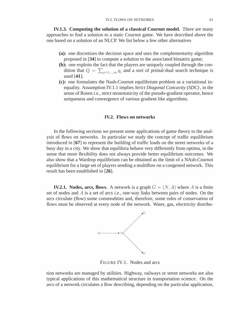
IV.2. FLOWS ON NETWORKS 61
IV.1.3. Computing the solution of a classical Cournot model.There are manyapproaches to find a solution to a static Cournot game. We have described above theone based on a solution of an NLCP. We list below a few other alternatives
(a): one discretizes the decision space and uses the complementarity algorithmproposed in [34] to compute a solution to the associated bimatrix game;
(b): one exploits the fact that the players are uniquely coupled through the con-dition thatQ =
∑j=1,...,m qj and a sort of primal-dual search technique is
used [41];(c): one formulates the Nash-Cournot equilibrium problem as a variational in-
equality. Assumption IV.1.1 impliesStrict Diagonal Concavity (SDC), in thesense of Roseni.e.,strict monotonicity of the pseudo-gradient operator, henceuniqueness and convergence of various gradient like algorithms.
IV.2. Flows on networks
In the following sections we present some applications of game theory to the anal-ysis of flows on networks. In particular we study the concept of traffic equilibriumintroduced in [67] to represent the building of traffic loads on the street networks of abusy day in a city. We show that equilibria behave very differently from optima, in thesense that more flexibility does not always provide better equilibrium outcomes. Wealso show that a Wardrop equilibrium can be obtained as the limit of a NAsh-Cournotequilibrium for a large set of players sending a multiflow on a congested network. Thisresult has been established in [26].
IV.2.1. Nodes, arcs, flows.A network is a graphG = (N,A) whereA is a finiteset of nodes andA is a set of arcsi.e., one-way links between pairs of nodes. On thearcs circulate (flow) some commodities and, therefore, some rules of conservation offlows must be observed at every node of the network. Water, gas, electricity distribu-
d - d¡¡
¡¡
¡µd
@@
@@
@R d
FIGURE IV.1. Nodes and arcs
tion networks are managed by utilities. Highway, railways or street networks are alsotypical applications of this mathematical structure in transportation science. On thearcs of a network circulates a flow describing, depending on the particular application,
62 IV. COURNOT AND NETWORK EQUILIBRIA
the volume of a commodity or the number of cars, trucks, trains that run on the arc dur-ing a specified unit of time. One denotesva the flow that circulates on the arca ∈ A.One associates alink traversal costSa(V ) with a flow vectorV = (va)a∈A circulatingon all the arcs. An example of such a cost function is the travel time needed by a unitof flow to go from the origin node to the end node of arca.
IV.2.2. Flow conservation rules.
IV.2.2.1. Simple flow conservation.We associate with any noden ∈ N two sub-sets of arcs
A+(n) :: the set of arcs with terminal nodenA−(n) :: the set of arcs with initial noden.
The simple flow conservation rule tells that theinflow to a node must be equal to theoutflowfrom this node, that is
(IV.8)∑
a∈A+(n)
va =∑
a∈A−(n)
va, ∀n ∈ N.
IV.2.2.2. Supply and demand.We associate with each noden ∈ N two numberssn anddn wheredn is the exogenous demand for the commodity in noden andsn isthe exogenous supply of commodity in that node. The flow conservation rule can nowbe extended as follows
(IV.9)∑
a∈A+(n)
va + sn =∑
a∈A−(n)
va + dn, ∀n ∈ N.
For example a gas utility has a network where some nodes are reservoirs and supplythe commodities, some other nodes are customers who consume the commodity, andfinally some node are only transshipment nodes where different pipes connect together.The delivery of gas will have to satisfy constraints of the form (IV.9) at every node1.
IV.3. Optimization and equilibria on networks
IV.3.1. The flow with minimal cost. We formulate the following problem
minV
∑a∈A
va Sa(V )(IV.10)
s.t.
dn − sn =∑
a∈A+(n)
va −∑
a∈A−(n)
va, ∀n ∈ N,(IV.11)
va ≥ 0.(IV.12)
1In that particular case one would have additional constraints due to the transmission of pressureinto the pipeline system; we shall not enter into this difficulty and refer the reader to [?] for more details.
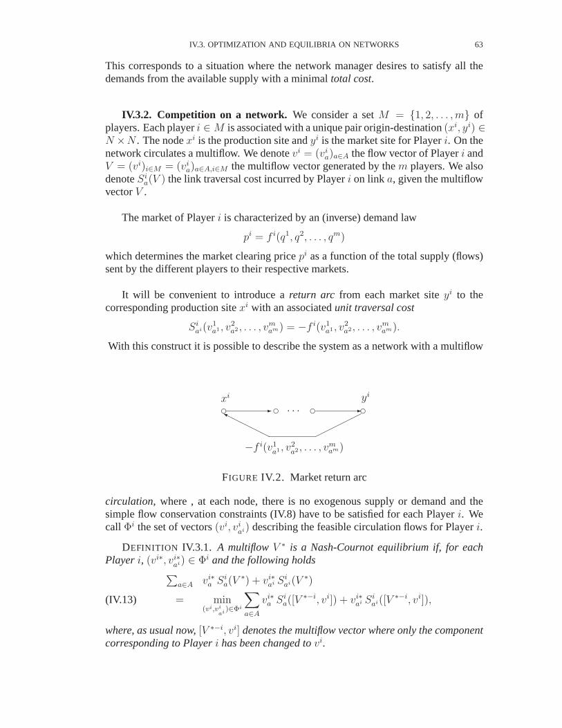
IV.3. OPTIMIZATION AND EQUILIBRIA ON NETWORKS 63
This corresponds to a situation where the network manager desires to satisfy all thedemands from the available supply with a minimaltotal cost.
IV.3.2. Competition on a network. We consider a setM = {1, 2, . . . ,m} ofplayers. Each playeri ∈ M is associated with a unique pair origin-destination(xi, yi) ∈N ×N . The nodexi is the production site andyi is the market site for Playeri. On thenetwork circulates a multiflow. We denotevi = (vi
a)a∈A the flow vector of Playeri andV = (vi)i∈M = (vi
a)a∈A,i∈M the multiflow vector generated by them players. We alsodenoteSi
a(V ) the link traversal cost incurred by Playeri on link a, given the multiflowvectorV .
The market of Playeri is characterized by an (inverse) demand law
pi = f i(q1, q2, . . . , qm)
which determines the market clearing pricepi as a function of the total supply (flows)sent by the different players to their respective markets.
It will be convenient to introduce areturn arc from each market siteyi to thecorresponding production sitexi with an associatedunit traversal cost
Siai(v1
a1 , v2a2 , . . . , vm
am) = −f i(v1a1 , v2
a2 , . . . , vmam).
With this construct it is possible to describe the system as a network with a multiflow
dxi
- d · · · d - dyi
©©©©©
−f i(v1a1 , v2
a2 , . . . , vmam)
HHHHHY
FIGURE IV.2. Market return arc
circulation, where , at each node, there is no exogenous supply or demand and thesimple flow conservation constraints (IV.8) have to be satisfied for each Playeri. Wecall Φi the set of vectors(vi, vi
ai) describing the feasible circulation flows for Playeri.
DEFINITION IV.3.1. A multiflowV ∗ is a Nash-Cournot equilibrium if, for eachPlayeri, (vi∗, vi∗
ai) ∈ Φi and the following holds∑
a∈A vi∗a Si
a(V∗) + vi∗
ai Siai(V ∗)
= min(vi,vi
ai )∈Φi
∑a∈A
vi∗a Si
a([V∗−i, vi]) + vi∗
ai Siai([V ∗−i, vi]),(IV.13)
where, as usual now,[V ∗−i, vi] denotes the multiflow vector where only the componentcorresponding to Playeri has been changed tovi.
64 IV. COURNOT AND NETWORK EQUILIBRIA
According to this definition, at equilibrium, each Playeri, minimizes a functionwhich is given by the sum of the traversal costs minus the total value of the sales of thecommodity flow he controls, given the flows decided by the other players.
It will be convenient to introduce the notations
J i(V ) =∑a∈A
via Si
a(V ) + viai Si
ai(V )
and to introduce ther-pseudo-gradient, wherer = (r1, r2, . . . , rm) ∈ IRm defined as
g(V, r) =
g1(V, r)g2(V, r)
...gm(V, r)
=
r1∇v1J1(V )r2∇v2J2(V )
...rm∇vmJm(V )
.
THEOREM IV.3.1. Assume that each payoff functionJ i is C1 and concave inv ∈Φi. ThenV ∗ is a Nash-Cournot equilibrium iff it satisfies the variational inequality
(IV.14) (V − V ∗)′g(V ∗, r) ≥ 0 ∀V ∈ Φ1 × Φ2 · · · × Φm.
Proof.This is a concave game. Apply Theorem Th-3.4.3. QED
THEOREM IV.3.2. Assume that each payoff functionJ i isC2 and there existsr > 0such that the symmetric matrix
[G(V, r) + G′(V, r)]
is negative definite, whereG(V, r) is the Jacobian of the pseudo-gradientg(V, r). Thenthe equilibrium is unique.
Proof.This is a concave gamea la Rosen. Apply Theorem III.4.2. QED
IV.3.3. Wardrop equilibrium on a network. There is a famous concept of trafficequilibrium introduced in [67]. In this problem one considers a networkG = (N, A).For each origin-destination pair(x, y) ∈ N × N there is transportation demand. Theimportant aspect of this demand is that it comes from a very large number of users, eachone contributing for a very small part of the demand. This corresponds approximatelyto the situation of the commuters traffic in peak hour of a working day. People living innodex go to work on nodey; each user has a single car which contributes marginallyto the traffic flow. We denotew = (wa)a∈A the flow that results from the commuterstravelling from their origins to their destinations. The question is to determine the floww that should result from a locally optimizing behavior of all users. Bylocally wemean an optimality which only concerns the particular user, given the behavior of allother users.
An important concept that enters into the definition of a traffic equilibrium is thenotion of a pathp linking the origin nodex to the destination nodey. Such a pathis a sequence of connected links, the first one having its initial node inx and the last

IV.3. OPTIMIZATION AND EQUILIBRIA ON NETWORKS 65
one its terminal node iny. A user who has to travel fromx to y selects a path. On
dx
- d · · · d - dy
dd ©©©©©*
· · ·HHHHHj
FIGURE IV.3. Paths fromx to y
each arca ∈ A, the link traversal is supposed to be influenced by the congestion of thenetworki.e.,we assume it to be a functionSa(w). The total travel time along a pathpis given by
∑a∈p Sa(w). The users, optimizing locally tend to select the path that has
the minimum total travel time to connect the originx to the destinationy. The conceptof Wardrop equilibrium is defined as follows
DEFINITION IV.3.2. A flow vectorw∗ is a Wardrop equilibrium if, for any pairorigin-destination(x, y), the following holds
∑a∈p∗
Sa(w∗) ≤
∑a∈p
Sa(w∗)(IV.15)
∀p∗ ∈ P ∗ p ∈ P,
whereP is the set of all possible paths fromx to y andP ∗ is the subset consisting ofall paths that are actually used (i.e., such that a positive flow is circulating on them).
One deduces immediately from this definition that, for all paths that are actuallyused between an originx and a destinationy, the total journey time is equal. Weeasily see that a Wardrop equilibrium corresponds to a situation where each user hasno incentive to modify the path he (she) is using for his (her) journey.
LEMMA IV.3.1. A Wardrop equilibrium flow vectorw∗ is characterized as the so-lution to the followingvariational inequality
(IV.16) (w − w∗)′S(w∗) ≤ 0 ∀w ∈ φ
whereφ is the set of all feasible flows.
Proof.
IV.3.4. Braess’ paradox. The so called Braess paradox [7], [24] illustrates wellthe difference between an optimal solution and an equilibrium solution.
Consider a highway network as in Figure IV.4. There are four origin-destinationpairs orlinks. A functionFk(x), k = 1 . . . K can be identified as a travel time through

66 IV. COURNOT AND NETWORK EQUILIBRIA
S T
F1(x)=10x
1 F
2(x)=25x
2+2
F4(x)=10x
4
F3(x)=x
3+50
A
B
FIGURE IV.4. A traffic network.
link k wherexk is the total flow assigned to this link; here,K = 4. The functionsFk(x) are increasing inx; clearly, the more traffic, the longer the journey.
The journey time is an obvious performance index for a commuter in this problem.Another index could the maintenance cost incurred by the local government. We willassume that thetotal system costis
(IV.17) J =K∑
k=1
xkFk(xk).
Suppose that the demand for travel from S to T is 3.6 . We will discuss what distributionof traffic is likely.
If the total traffic went through the upper links 1 and 2 only the travel time would be128.5 . Conversely, if everybody used links 3 and 4 the journey would last 89.6 . Thetotal costs would be 460.80 and 322.56 , respectively. See the second and third columnsin Table IV.1 (the subsequent columns show other solutions obtained by using differentperformance indices). Obviously, by sharing the upper and bottom links these timesand costs could be improved.
If the customers of this highway network could see what the current traffic on eachlink were they would try to minimize their travel times until anequilibrium wouldestablish itself. At this equilibrium, the journey times through 1-2 and 3-4 would beequalled. Hence, the following equations have to be satisfied for the equilibrium to

IV.3. OPTIMIZATION AND EQUILIBRIA ON NETWORKS 67
1-2 3-4 equil. min cost min cost(+5) equil.(+5) ºequil.(+5)
x1 SA 3.6 0 1.9 1.38 2.06 3.6 2.24x2 AT 3.6 0 1.9 1.38 1.17 1.32 1.63x3 SB 0 3.6 1.7 2.22 1.54 0 1.36x4 BT 0 3.6 1.7 2.22 2.43 2.28 1.97x5 AB n.a. n.a. n.a. n.a. .89 2.28 .61max time 128.5 89.6 68.7 74.4 75.9 71.1 71.1
cost 460.80 322.56 247.1 234.6 227.12 255.8 235.0
TABLE IV.1. Various traffic intensities and the corresponding payoffs.
exist:
10x1 + 25x2 + 2 = x3 + 50 + 10x4(IV.18)
x1 − x2 = 0(IV.19)
x3 − x4 = 0(IV.20)
x1 + x3 = 3.6 .(IV.21)
The solution to (IV.18)-(IV.21) and the corresponding time and cost are shown in col-umn four of Table IV.1.
Let us see now what the local government preferred solution is. This will be ob-tained by solving the following minimization problem
min4∑
k=1
xkFk(xk)(IV.22)
s.t. (IV.19)− (IV.21) hold .
The solution to (IV.22) is presented in column five. Clearly, the traffic through thequickly saturating (and expensive) link AT has easied. The maximum journey timegiven in the table is through links 3-4; the other link’s time is 50.5 .
There is a clear difference between the equilibrium solution that minimizes thetravel time (equilibrium) and the local government’s cost minimizing solution. In thecommuter preferred solution there is a lot of traffic through links 1-2 and less trafficthrough links 3-4. The local government might consider a quick link AB as in FigureIV.5 (not to scale!) in an attempt to improve the situation by redirecting some trafficaway from the congested AT toward the under-utilized BT.
Suppose that the local government has built the link AB, see Figure IV.5, in theexpectation to diminish the traffic through AT.

68 IV. COURNOT AND NETWORK EQUILIBRIA
S T
F1(x)=10x
1 F
2(x)=25x
2+2
F4(x)=10x
4
F3(x)=x
3+50
A
B
F5(x)=
x5+10
FIGURE IV.5. An extended traffic network.
Let us solve the problem of the cost minimization with the fifth link added to thenetwork as follows:
min5∑
k=1
xkFk(xk)(IV.23)
s.t.
x1 = x2 + x5(IV.24)
x4 = x3 + x5(IV.25)
x1 + x3 = 3.6 .(IV.26)
The solution is presented in column six. Apparently, this solution gives the lowestgovernment cost so, the link utilization must be more equilibrated than without theAB link. However, the maximum travel time (through 3-4) grows while the remaininglinks travel times are: 51.8 (1-2) and 56.5 (1-3-4).
This solution gives longer journey times for commuters travelling through the links3-4 than without the AB connection. The commuters will obviously seek to improvethese times until an equilibrium is achieved.
Unfortunately, there is no “global” equilibrium, which would make the travel times1-2, 1-5-4 and 3-4 identical. This is obvious as the following system of equations , hasno positive solution:
10(x11 + x12) + 25x11 + 2 = 10(x11 + x12) + x12 + 10 + 10(x12 + x3)(IV.27)
10(x11 + x12) + 25x11 + 2 = x3 + 50 + 10(x12 + x3)(IV.28)
x11 + x12 + x3 = 3.6(IV.29)
wherex11 + x12 = x1 is the traffic through SA. Neither the travel times through 1-5-4and 3-4 can be equalized. The only equilibrium, which can be established is such that
IV.4. A CONVERGENCE RESULT 69
the journey times through 1-5-4 and 1-2 are the same and no traffic passes through SB.Indeed, the system
10(x11 + x12) + x11 + 10 + 10x11 = 10(x11 + x12) + 25x12 + 2(IV.30)
10(x11 + x12) + 25x11 + 2 = x3 + 50 + 10(x12 + x3)(IV.31)
x11 + x12 = 3.6(IV.32)
has a unique solution which is written in column seven of Table IV.1. Here is theparadox, the travellers are worse off than without the link AB! Also surprisingly, itis uneconomical for a single commuter to start the journey using link SB. Indeed,x + 50 > 11x + 10 for ∀x < 4.2
The authors of [30] point to the fact that more options mean more strategies andmore equilibria. The Breass paradox illustrates the fact that, in a new equilibrium, allplayers may be worse off. The authors of [30] also notice certain similarity betweenBreass’ paradox and the prisoner’s dilemma (see Example III.3.3, page 34); the latterexists because each prisoner’s strategy space contains two options. In other words,there would be no dilemma and the payoffs (2,2) would be a unique equilibrium if theplayers had just one option of no cooperating (e.g.,if they spoke a different languagethan the police), see Table III.1 page 34.
IV.4. A convergence result
We address the following question
is it possible to approximate a Wardrop equilibrium floww∗ by thetotal flow w∗(n) resulting from a Nash-Cournot equilibrium for thegame played on the networkG by nm players partitioned intomclassesIi, i ∈ M , where a class corresponds to a particular origin-destination pair(xi, yi)?
IV.4.1. The approximating games.We call Γ(n) the game defined on the net-workG in the following way. There arem origin-destination pairs(xi, y), i = 1, 2, . . . , m.With eachi is associated a setMi of n identical players who share the same link tra-versal cost functionSa(w) and the same demand lawf i(q1, q2, . . . , qm), where
qi =∑
`∈M i
v`ai , i = 1, 2, . . . , m.
We remind the reader that the arcai is the return link between the market siteyi andthe production sitexi.
2Many traffic intensity distributions could weakly dominate the equilibrium; for a result of that kindsee the last column in Table IV.1. The equilibrium domination is called ageneralized Breass’ paradox[24].

70 IV. COURNOT AND NETWORK EQUILIBRIA
We assume that the commodities produced and marketed by thenm players arehomogenous and we call
wa =∑
`=1,...,nm
v`a
the total flow circulating on the arca. The payoff of Player ∈ Mi is therefore givenby
(IV.33) J `(v1, v2, . . . , vmn) = v`aif i(q1, q2, . . . , qm)−
∑a∈A
v`aSa(w).
If we extend the arc setA to also contain the return arcsai, i ∈ M , with an associatedtraversal costSai(V ) = −f i(q1, q2, . . . , qm), we can rewrite the payoff functions inthe more compact form
(IV.34) J `(v1, v2, . . . , vmn) = −∑a∈A
v`aSa(w).
We shall now characterize the Nash-Cournot equilibrium through the associated vari-ational inequality and use this formulation to prove the convergence to a limit whichcorresponds to a Wardrop-like equilibrium.
LEMMA IV.4.1. Assume that all traversal cost functions areC1, and the payofffunction of each Player is concave inv`. Then a Nash-Cournot equilibrium(v`∗(n),` = 1, . . . , nm, for the gameΓ(n) is characterized by the variational inequality
(IV.35) (v`∗(n)− v`)′(S(w∗(n)) + (∇S(w∗(n)))′v`∗(n) ≤ 0
∀v` ∈ Φ` ∀` ∈ Mi, i = 1, . . . , m.
Proof.Explicit the condition established in Theorem IV.3.1. QED
We are now ready to prove the main result
THEOREM IV.4.1. Under the assumptions of Lemma IV.4.1there exists a Wardropequilibrium on the networkG, with flow vectorw∗ and a sequence{Γ(n)}n∈IN ofgames onG admitting Nash equilibria multiflowV ∗(n), such that the resulting totalflow vectorsw∗
a(n) =∑
`=1,...,nm v`∗a (n), a ∈ A, verify
limn→∞
w∗(n) = w∗.
Proof.For eachn the gameΓ(n) admits a Nash-Cournot equilibrium multiflowV ∗(n). Since all the players inM i are supposed to be identical we can aleays assumethat all the players inM i share the same strategy and, therefore, we can write
v`∗(n) =1
nωi∗(n), ∀` ∈ M i
whereωi∗(n) is a flow which is uniformly bounded. The associated total link-flowvector
w∗a(n) =
∑
`=1,...,nm
v`∗a (n) =
m∑i=1
ωi∗(n)

IV.4. A CONVERGENCE RESULT 71
is also uniformly bounded. Hence, asn tends to∞, one can extract a convergingsubsequence (still denoted byn for the sake of simplifying the notations) with a limitdenotedw∗.
Replacingv`∗(n) by 1n
ωi∗(n) in (IV.35) and summing over all players, there comes
(w∗(n)− w)′(S(w∗(n)) + Qn ≤ 0 ∀w ∈ φ
with
Qn =m∑
i=1
∑
`∈M i
(ωi∗(n)
n− v`
)(∇S(w∗(n)))′
ωi∗(n)
n.
Now, since the set of feasible flowsφ is compact, one haslimn→∞ Qn = 0, thereforethe limit flow vectorw∗ satisfies
(w∗ − w)′S(w∗) ≤ 0 ∀w ∈ φ
and this is by Lemma IV.3.1 a Wardrop equilibrium. QED


Part 2
Repeated and sequential Games


CHAPTER V
Repeated Games and Memory Strategies
In this chapter we begin our analysis of “dynamic games”. To say it in an imprecisebut intuitive way, the dynamic structure of a game expresses a change over time of theconditions under which the game is played. In a repeated game this structural changeover time is due to the accumulation of information about the “history” of the game. Astime unfolds the information at the disposal of the players changes and, since strategiestransform this information into actions, the players’ strategic choices are affected. Ifa game is repeated twicei.e., the same game is played in two successive stages and areward is obtained at each stage, one can easily see that, at the second stage, the playerscan decide on the basis of the outcome of the first stage. The situation becomes moreand more complex as the number of stages increases, since the players can base theirdecisions onhistories represented by sequences of actions and outcomes observedover increasing numbers of stages. We may also consider games that are played over aninfinite number of stages. These infinitely repeated games are particularly interesting,since, at each stage, there is always an infinite number of remaining stages over whichthe game will be played and, therefore, there will not be the so-called “end of horizoneffect” where the fact that the game is ending up affects the players behavior. Indeed,the evaluation of strategies will have to be based on the comparison of infinite streamsof rewards and we shall explore different ways to do that. In summary, the importantconcept to understand here is that, even if it is the “same game” which is repeated overa number of periods, the global “repeated game” becomes a fully dynamic system witha much more complex strategic structure than the one-stage game.
In this chapter we shall consider repeated bimatrix games and repeated concavem-player games. We shall explore, in particular, the class of equilibria when the numberof periods over which the game is repeated (thehorizon) becomes infinite. We willshow how the class of equilibria in repeated games can be expended very much if oneallows memory in the information structure. The class ofmemory strategiesallows theplayers to incorporatethreats in their strategic choices. A threat is meant to deter theopponents to enter into a detrimental behavior. In order to be effective a threat must becredible. We shall explore the credibility issue and show how the subgame perfectnessproperty of equilibria introduces a refinement criterion that make these threats credible.
Notice that, at a given stage, the players actions have no direct influence on thenormal form description of the games that will be played in the forthcoming periods. Amore complex dynamic structure would obtain if one assumes that the players actionsat one stage influence the type of game to be played in the next stage. This is the case
75

76 V. REPEATED GAMES AND MEMORY STRATEGIES
for the class ofMarkovor sequentialgames and a fortiori for the class ofdifferentialgames, where the time flows continuously. These dynamic games will be discussed insubsequent chapters of this volume.
V.1. Repeating a game in normal form
Repeated games have been also calledgames in semi-extensive formin [21]. Indeedthis corresponds to an explicit dynamic structure, as in the extensive form, but with agame in normal form defined at each period of time. In the repeated game, the globalstrategy becomes a way to define the choice of a stage strategy at each period, onthe basis of the knowledge accumulated by the players on the ”history” of the game.Indeed the repetition of the same game in normal form permits the players to adapt theirstrategies to the observed history of the game. In particular, they have the opportunityto implement a class of strategies that incorporate threats.
The payoff associated with a repeated game is usually defined as the sum of thepayoffs obtained at each period. However, when the number of periods tends to∞, atotal payoff that implies an infinite sum may not converge to a finite value. There areseveral ways of dealing with the comparison of infinite streams of payoffs. We shalldiscover some of them in the subsequent examples.
V.1.1. Repeated bimatrix games.Figure V.1 describes a repeated bimatrix gamestructure. The same matrix game is played repeatedly, over a numberT of periods or
1 · · · q
1 (αj11)j=1,2 · · · (αj
1q)j=1,2...
......
...p (αj
p1)j=1,2 · · · (αjpq)j=1,2
-
1 · · · q
1 (αj11)j=1,2 · · · (αj
1q)j=1,2...
......
...p (αj
p1)j=1,2 · · · (αjpq)j=1,2
- · · ·
FIGURE V.1. A repeated game
stagesthat represent the passing of time. In the one-stage game, where Player 1 hasppure strategies and Player 2q pure strategies and the one-stage payoff pair associatedwith the startegy pair(k, `) is given by(αj
k`)j=1,2. The payoffs are accumulated overtime. As the players may recall the past history of the game, the extensive form of thoserepeated games is quite complex. The game is defined in asemi-extensive formsinceat each period a normal form (i.e.,an already aggregated description) defines the con-sequences of the strategic choices in a one-stage game. Even if the same game seemsto be played at each period (it is similar to the others in its normal form description), infact, the possibility to use the history of the game as a source of information to adaptthe strategic choice at each stage makes a repeated game a fully dynamic “object”.

V.1. REPEATING A GAME IN NORMAL FORM 77
We shall use this structure to prove an interesting result, called the “folk theorem”,which shows that we can build an infinitely repeated bimatrix game, played with thehelp of finite automata, where the class of equilibria permits the approximation of anyindividually rational outcome of the one-stage bimatrix game.
V.1.2. Repeated concave games.Consider now the class of dynamic games whereone repeats a concave gamea la Rosen. Lett ∈ {0, 1, . . . , T − 1} be the time index.At each time periodt the players enter into a noncooperative game defined by
(M ; Uj, ψj(·), j ∈ M)
where as indicated in section III.4,M = {1, 2, . . . , m} is the set of players,Uj isa compact convex set describing the actions available to Playerj at each period andψj(u(t)) is the payoff to Playerj when the action vectoru(t) = (u1(t), . . . , um(t)) ∈U = U1 × U2 × · · · × Um is chosen at periodt by them players. This function isassumed to be concave inuj.
We shall denoteu = (u(t) : t = 0, 1 . . . , T − 1) the actions sequence over thesequence ofT periods. The total payoff of Playerj over theT -horizon is then definedby
(V.1) V Tj (u) =
T−1∑t=0
ψj(u(t)).
V.1.2.1. Open-loop information structure.At period t, each Playerj knows onlythe current timet and what he has played in periodsτ = 0, 1, . . . , t − 1. He does notobserve what the other players do. We implicitly assume that the players cannot usethe rewards they receive at each period toinfer throughe.g.,an appropriate filtering theactions of the other players. Theopen-loopinformation structure actually eliminatesalmost every aspect of the dynamic structure of the repeated game context.
V.1.2.2. Closed-loop information structure.At period t, each Playerj knows notonly the current timet and what he has played in periodsτ = 0, 1, . . . , t− 1, but alsowhat the other players have done at previous period. We callhistory of the game atperiodτ the sequence
h(τ) = (u(t) : t = 0, 1 . . . , τ − 1).
A closed-loop strategy for Playerj is defined as a sequence of mappings
γτj : h(τ) 7→ Uj.
Due to the repetition over time of the same game, each Playerj can adjust his choiceof one-stage actionuj to the history of the game. This permits the consideration ofmemory strategieswhere some threats are included in the announced strategies. Forexample, a player can declare that some particular histories would “trigger” aretalia-tion from his part. The description of atrigger strategywill therefore include

78 V. REPEATED GAMES AND MEMORY STRATEGIES
• a nominal “mood” of play that contributes to the expected or desired outcomes• a retaliation “mood” of play that is used as a threat• the set of histories that trigger a switch from thenominal mood of playto the
retaliation mood of play.
Many authors have studied equilibria obtained in repeated games through the use oftrigger strategies(see for example [51], [52], [22]).
V.1.2.3. Infinite horizon games.If the game is repeated over an infinite numberof periods then payoffs are represented by infinite streams of rewardsψj(u(t)), t =1, 2, . . . ,∞.
Discounted sum of rewards:We have assumed that the actions setsUj are compact,therefore, since the functionsψj(·) are continuous, the one-stage rewardsψj(u(t)) areuniformly bounded. Hence, the discounted payoffs
(V.2) Vj(u) =∞∑
t=0
βtjψj(u(t)),
whereβj ∈ [0, 1) is the discount factor of Playerj, are well defined. Therefore, if theplayers discount over time, we can compare strategies on the basis of the discountedsums of the rewards they generate for each player.
Average rewards per period:If the players do not discount over time the compari-son of strategies imply the consideration of infinite streams of rewards that sum up toinfinity. A way to circumvent the difficulty is to consider alimit average reward perperiod in the following way
(V.3) gj(u) = lim infT→∞
1
T
T−1∑t=0
ψj(u(t)).
To link this evaluation of infinite streams of rewards with the previous one based ondiscounted sums one may define theequivalent discounted constant reward
(V.4) gβj
j (u) = (1− βj)∞∑
t=0
βtjψj(u(t)).
One expects that, for well behaved games, the following limiting property holds true
(V.5) limβj→1
gβj
j (u) = gj(u).
V.1.2.4. Threats. In infinite horizon repeated games each player has alwaysenoughtime to retaliate. He will always have the possibility to implement an announced threat,if the opponents are not playing according to somenominal sequencecorresponding toan agreement. We shall see that the equilibria, based on the use ofthreatsconstitute avery large class. Therefore the set of strategies with thememoryinformation structureis much more encompassing than theopen-loopone.

V.2. FOLK THEOREM 79
V.1.2.5. Existence of a “trivial” dynamic equilibrium.We know, by Rosen’s ex-istence theorem, that a concave ”static game”
(M ; Uj, ψj(·), j ∈ M)
admits an equilibriumu∗. It should be clear (see exercise 4.1) that the sequenceu∗ =(u(t) ≡ u∗ : t = 0, 1 . . . , T − 1) is also an equilibrium for the repeated game in boththe open-loop and closed-loop (memory) information structure.
Assume the one period game is such that a unique equilibrium exists. The open-loop repeated game will also have a unique equilibrium, whereas the closed-loop re-peated game will still have a plethora of equilibria, as we shall see it shortly.
V.2. Folk theorem
In this section we present the celebratedfolk theorem. This name is due to thefact that there is no well defined author of the first version of it. The idea is that aninfinitely repeated game should permit the players to design equilibria, supported bythreats, with outcomes being Pareto efficient. The strategies will be based onmemory,each player remembering the past moves of game. Indeed the infinite horizon couldgive raise to an infinite storage of information, so there is a question of designingstrategies with the help of mechanisms that would exploit the history of the game butwith a finite information storage capacity. Finite automata provide such systems.
V.2.1. Repeated games played by automata.A finite automatonis a logical sys-tem that, when stimulated by aninput, generates anoutput. For example an automatoncould be used by a player to determine the stage-game action he takes given the in-formation he has received. The automaton is finite if the length of the logical input (astream of0 − 1 bits) it can store is finite. So in our repeated game context, a finiteautomaton will not permit a player to determine his stage-game action upon an infinitememory of what has happened before. To describe a finite automaton one needs thefollowing
• A list of all possible stored input configurations; this list is finite and eachelement is called astate. One element of this list is theinitial state.
• An output function determines the action taken by the automaton, given itscurrent state.
• A transition function tells the automaton how to move from one state to an-other after it has received a new input element.
In our paradigm of a repeated game played by automata, the input element for theautomatona of Player 1 is the stage-game action of Player 2 in the preceding stage,and symmetrically for Player 2. In this way, each player can choose a way to processthe information he receives in the course of the repeated plays, in order to decide thenext action.

80 V. REPEATED GAMES AND MEMORY STRATEGIES
An important aspect of finite automata is that, when they are used to play a repeatedgame, they necessarily generate cycles in the successive states and hence in the actionstaken in the successive stage-games.
Let G be a finite two player gamei.e., a bimatrix game, which defines the one-stage game.U andV are the sets of pure strategies in the gameG for Player 1 and 2respectively. Denote bygj(u, v) the payoff to Playerj in the one-stage game when thepure strategy pair(u, v) ∈ U × V has been selected by the two players.
The game is repeated indefinitely. Although the set of strategies for an infinitelyrepeated game is enormously rich, we shall restrict the strategy choices of the playersto the class of finite automata. A pure strategy for Player 1 is an automatona ∈ Awhich has for input the actionsu ∈ U of Player 2. Symmetrically a pure strategy forPlayer 2 is an automatonb ∈ B which has for input the actionsv ∈ V of Player 1.
We associate with the pair of finite automata(a, b) ∈ A × B a pair of averagepayoffs per stage defined as follows
(V.6) gj(a, b) =1
N
N∑n=1
gj(un, vn) j = 1, 2,
whereN is the length of the cycle associated with the pair of automata(a, b) and(un, vn) is the action pair at then-th stage in this cycle. One notices that the expression(V.6) is also the limit average reward per period due to the cycling behavior of the twoautomata.
We callG the game defined by the strategy setsA andB and the payoff functions(V.6).
V.2.2. Minimax point. Assume Player 1 wants to threaten Player 2. An effectivethreat would be to define his action in a one-stage game through the solution of
m2 = minu
maxv
g2(u, v).
Similarly if Player 2 wants to threaten Player 2, an effective threat would be to definehis action in a one-stage game through the solution of
m1 = minv
maxu
g1(u, v).
We callminimax pointthe pairm = (m1, m2) in IR2.
V.2.3. Set of outcomes dominating the minimax point.
V.2. FOLK THEOREM 81
THEOREM V.2.1. LetPm be the set of outcomes in a matrix game that dominatethe minimax pointm. Then the outcomes corresponding to Nash equilibria in purestrategies1 of the gameG are dense inPm.
Proof: Let g1,g2, . . . ,gK be the pairs of payoffs that appear in the bimatrix gamewhen it is written in the vector form, that is
gk = (g1(uk, vk), g2(uk, vk))
where(uk, vk) is a possible pure strategy pair. Letq1, q2, . . . , qK be nonnegative ratio-nal numbers that sum to 1. Then the convex combination
g∗ = q1g1 + q2g2, . . . , qKgK
is an element ofP if g∗1 ≥ m1 andg∗2 ≥ m2 . The set of theseg is dense inP. Eachqk
being a rational number can be written as a ratio of two integers, that is a fraction. It ispossible to write theK fractions with a common denominator, hence
qk =nk
N,
withn1 + n2 + · · ·+ nK = N
since theqk’s must sum to 1.
We construct two automataa∗ andb∗, such that, together, they play(u1, v1) dur-ing n1 stages,(u2, v2) duringn2 stages,etc.They complete the sequence by playing(uK , vK) duringnK stages and theN -stage cycle begins again. The limit average perperiod reward of Playerj in theG game played by these automata is given by
gj(a∗, b∗) =
1
N
K∑
k=1
nkgj(uk, vk) =K∑
k=1
qkgj(uk, vk) = g∗j .
Therefore these two automata will achieve the payoff pairg. Now we refine the struc-ture of these automata as follows:
• Let u(n) andv(n) be the pure strategy that Player 1 and Player 2 respectivelyare supposed to play at stagen, according to the cycle defined above.
• The automatona∗ playsu(n+1) at stagen+1 if automatonb has playedv(n)at stagen; otherwise it playsu, the strategy that is minimaxing Player 2’s oneshot payoff and this stage strategy will be played forever.
• Symmetrically, the automatonb∗ playsv(n + 1) at stagen + 1 if automatonahas playedu(n) at stagen; otherwise it playsv, the strategy that is minimax-ing Player 1’s one shot payoff and this stage strategy will be played forever.
It should be clear that the two automataa∗ andb∗ defined as above constitute a Nashequilibrium for the repeated gameG wheneverg is dominatingm i.e.,g ∈ Pm. Indeed,
1A pure strategy in the gameG is a deterministic choice of an automaton; this automaton willprocess information coming from the repeated use of mixed strategies in the repeated game.

82 V. REPEATED GAMES AND MEMORY STRATEGIES
if Player 1 changes unilaterally his automaton toa then the automatonb∗ will selectfor all periods, except a finite number, the minimax actionv and, as a consequence, thelimit average per period reward obtained by Player 1 is
g1(a, b∗) ≤ m1 ≤ g1(a∗, b∗).
Similarly for Player 2, a unilateral change tob ∈ B leads to a payoff
g2(a∗, b) ≤ m2 ≤ g2(a
∗, b∗).
Q.E.D.
REMARK V.2.1. This result is known as the folk theorem, because it has alwaysbeen in the ”folklore” of game theory without knowing to whom it should be attributed.
The class of equilibria is more restricted if one imposes a condition that the threatsused by the players in their announced strategies have to becredible. This is the issuediscussed in one of the following sections under the name ofsubgame perfectness.
V.3. Collusive equilibrium in a repeated Cournot game
V.3.1. Infinite horizon and Cournot equilibrium threats. Consider a Cournotoligopoly game repeated over an infinite sequence of periods. Lett = 1, . . . ,∞ be thesequence of time periods. Letq(t) ∈ IRm be the production vector chosen by themfirms at periodt andψj(q(t)) the payoff to Playerj at periodt.
We denoteq = q(1), . . . ,q(t), . . .
the infinite sequence of production decisions of them firms. Over the infinite timehorizon the rewards of the players are defined as
Vj(q) =∞∑
t=0
βtjψj(q(t))
whereβj ∈ [0, 1) is a discount factor used by Playerj.
We assume that, at each periodt, all players have the same informationh(t) whichis the history of passed productions decided by all the firms in competition, that ish(t) = (q(0),q(1), . . . ,q(t− 1)).
We consider, for the one-stage game, two possible outcomes,
(i): the Cournot equilibrium, supposed to be uniquely defined byqc = (qcj)j=1,...,m
and(ii): a Pareto outcome resulting from the production levelsq∗ = (q∗j )j=1,...,m and
such thatψj(q)∗ ≥ ψj(qc), j = 1, . . . , m. We say that this Pareto outcome is
acollusive outcome dominating the Cournot equilibrium.
V.3. COLLUSIVE EQUILIBRIUM IN A REPEATED COURNOT GAME 83
A Cournot equilibrium for the repeated game is defined by the strategy consistingfor each Playerj to choose repeatedly the production levelsqj(t) ≡ qc
j , j = 1, 2. How-ever there are many other equilibria that can be obtained through the use of memorystrategies.
Let us define
V ∗j =
∞∑t=0
βtjψj(q
∗)(V.7)
Φj(q∗) = max
qj
ψj([q∗(−j), qj]).(V.8)
The following has been shown in [21]
LEMMA V.3.1. There exists an equilibrium for the repeated Cournot game thatyields the payoffsV ∗
j if the following inequality holds
(V.9) βj ≥ Φj(q∗)− ψj(q
∗)Φj(q∗)− ψj(qc)
.
This equilibrium is reached through the use of a so-called trigger strategy defined asfollows(V.10)
if (q(0),q(1), . . . ,q(t− 1)) = (q∗,q∗, . . . ,q∗) thenqj(t) = q∗jotherwise qj(t) = qc
j .
}
Proof: If the players play according to (V.10) the payoff they obtain is given by2
V ∗j =
∞∑t=0
βtjψj(q
∗) =1
1− βj
ψj(q∗).
Assume Playerj decides to deviate unilaterally at period 0. He knows that his deviationwill be detected at period 1 and that, thereafter the Cournot equilibrium productionlevelqc will be played. So, the best he can expect from this deviation is the followingpayoff which combines the maximal reward he can get in period 0 when the other firmsplay q∗k with the discounted value of an infinite stream of Cournot outcomes3.
Vj(q) = Φj(q∗) +
βj
1− βj
ψj(qc).
This unilateral deviation is not profitable if
Vj(q) ≤ V ∗j =
∞∑t=0
βtjψj(q
∗) =1
1− βj
ψj(q∗),
that is, if the following inequality holds
ψj(q∗)− Φj(q
∗) +βj
1− βj
(ψj(q∗)− ψj(q
c)) ≥ 0,
2We use here the fact that the∑∞
k=0 βk = 11−β whenβ < 1.
3We use here the fact that the∑∞
k=1 βk = β1−β whenβ < 1.

84 V. REPEATED GAMES AND MEMORY STRATEGIES
which can be rewritten as
(1− βj)(ψj(q∗)− Φj(q
∗)) + βj(ψj(q∗)− ψj(q
c)) ≥ 0,
from which we get
ψj(q∗)− Φj(q
∗)− βj(ψj(qc)− Φj(q
∗)) ≥ 0.
and, finally the condition (V.9)
βj ≥ Φj(q∗)− ψj(q
∗)Φj(q∗)− ψj(qc)
.
The same reasonning holds if the deviation occurs at any other periodt. Q.E.D.
REMARK V.3.1. According to this strategy theq∗ production levels correspond toa cooperative mood of play while theqc correspond to apunitivemood of play. Thepunitive mood is athreat. As the punitive mood of play consists to play the Cournotsolution which is indeed an equilibrium, it is a credible threat. Therefore the playerswill always choose to play in accordance with the Pareto solutionq∗ and thus theequilibrium defines a nondominated outcome.
V.3.2. Subgame perfectness.It is important to notice the difference between thethreats used in the folk theorem and the ones used in this repeated Cournot game. Inthe folk theorem, the threats are the “most effective ones” in the sense that the threatsaims at maximizing the damage done to the opponent. However, as already mentionedthese threats lack credibility since, for the player who is using the threats, this actionis not the best course of action, given the opponent behavior.
In the infinitely repeated Cournot game, the threats constite also an equilibrium forthe dynamic game. Therefore the threats are credible, since, once the threats are ap-plied by every player, everyone is reacting optimally to the actions of the other players.We say that the memory (trigger strategy) equilibrium issubgame perfectin the senseof Selten [56].
V.3.3. Finite vs infinite horizon. There is an important difference between finitelyand infinitely repeated games. If the same game is repeated only a finite number oftimes then, in a subgame perfect equilibrium, a single game equilibrium will be re-peated at each period. This is due to the impossibility to retaliate at the last period.Then this situation is translated backward in time until the initial period. When thegame is repeated over an infinite time horizon there is always enough time to retaliateand even, possibly, to resume cooperation. For example, let us consider a repeatedCournot game, without discounting where the players’ payoffs are determined by thelong term average of the one sage rewards. If the players haveperfect informationwith delaythey can observe without errors the moves selected by their opponents inprevious stages. There might be a delay of several stages before this observation ismade. In that case it is easy to show that, to any cooperative solution dominating astatic Nash equilibrium corresponds a subgame perfect sequential equilibrium for therepeated game, based on the use oftrigger strategies. These strategies use as a threat

V.4. EXERCISES 85
a switch to the noncooperative solution for all remaining periods, as soon as a playerhas been observed not to play according to the cooperative solution. Since the longterm average only depends on the infinitely repeated one stage rewards, it is clear thatthe threat gives raise to the Cournot equilibrium payoff in the long run. This is thesubgame perfect version of thefolk theorem[22].
V.3.4. A repeated stochastic Cournot game with discounting and imperfectinformation. We give now an example of stochastic repeated game for which theconstruction of equilibria based on the use of threats is not trivial. This is the stochasticrepeated game, based on the Cournot model with imperfect information, (see [23],[50]).
Let X(t) =∑m
j=1 xj(t) be the total supply ofm firms at timet and θ(t) be asequence of i.i.d4 random variables affecting these prices. Each firmj chooses itssuppliesxj(t) ≥ 0, in a desire to maximize its total expected discounted profit
Vj(x1(·), . . . , xj(·), . . . , xm(·)) = Eθ
∞∑t=0
βt[D(X(t), θ(t))xj(t)− cj(xj(t))],
j = 1, . . . ,m,
whereβ < 1 is the discount factor. The assumed information structure does not alloweach player to observe the opponent actions used in the past. Only the sequence ofpast prices, corrupted by the random noise, is available. Therefore the players cannotmonitor without error the past actions of their opponent(s). This impossibility to detectwithout error a breach of cooperation increases considerably the difficulty of buildingequilibria based on the use of credible threats. In [23], [50] it is shown that there existsubgame perfect equilibria, based on the use oftrigger strategies, which are dominat-ing the repeated Cournot-Nash equilibrium. This construct uses the concept of Markovgame and will be further discussed in Part 3 of these Notes. It will be shown that theseequilibria are in fact closely related to the so-calledcorrelatedand/orcommunicationequilibria discussed at the end of Part 2.
V.4. Exercises
Exercise 5.1.Prove that the repeated one-stage equilibrium is an equilibrium forthe repeated game with additive payoffs and a finite number of periods. Extend theresult to infinitely repeated games.
Exercise 5.2.Show that condition (V.9) holds ifβj = 1. Adapt Lemma V.3.1 to thecase where the game is evaluated through the long term average reward criterion.
4Independent and identically distributed.


CHAPTER VI
Shapley’s Zero Sum Markov Game
VI.1. Process and rewards dynamics
The concept ofMarkov gamehas been introduced, in a zero-sum game framework,in [57]. The structure of this game can also be described as acontrolled Markov chainwith two competing agents.
Let S = {1, 2, . . . , n} be the set of possible states of a discrete time stochasticprocess{x(t) : t = 0, 1, . . . }. Let Uj = {1, 2, . . . , λj}, j = 1, 2, be the finiteactionsetsof two players. The process dynamics is described by thetransition probabilities
ps,s′(u) = P[x(t + 1) = s′|x(t) = s, u], s, s′ ∈ S, u ∈ U1 × U2,
which satisfy, for allu ∈ U1 × U2
ps,s′(u) ≥ 0∑
s′∈S
ps,s′(u) = 1, s ∈ S.
As the transition probabilities depend on the players actions we speak of acontrolledMarkov chain. A transition reward function
r(s,u), s ∈ S, u ∈ U1 × U2,
defines the gain of Player 1 when the process is in states and the two players take theaction pairu. Player 2’s reward is given by−r(s,u), since the game is assumed to bezero-sum.
VI.2. Information structure and strategies
VI.2.1. The extensive form of the game.The game defined above corresponds toa game in extensive form with an infinite number of moves. We assume an informationstructure where the players choosesequentiallyandsimultaneously, with perfect recall,their actions. This is illustrated in figure VI.1
VI.2.2. Strategies. A strategy is a device which transforms the information intoaction. Since the players may recall the past observations, the general form of a strat-egy can be quite complex.
87

88 VI. SHAPLEY’S ZERO SUM MARKOV GAME
µ´¶³s - P1
¢¢¢¢¢¢¢¢¢¢
u11
AAAAAAAAAAU
u21
¾
½
»
¼
P2
P2
¡¡
¡¡
¡µ
u12
@@
@@
@Ru2
2
¡¡
¡¡
¡µ
u12
@@
@@
@Ru2
2
µ´¶³E ©©©©©*ps,·(u)
HHHHHj
-
ps,·(u)
µ´¶³·
µ´¶³·
µ´¶³·
µ´¶³E ©©©©©*ps,·(u)
HHHHHj
-
ps,·(u)
µ´¶³·
µ´¶³·
µ´¶³·
µ´¶³E ©©©©©*ps,·(u)
HHHHHj
-
ps,·(u)
µ´¶³·
µ´¶³·
µ´¶³·
µ´¶³E ©©©©©*ps,·(u)
HHHHHj
-
ps,·(u)
µ´¶³·
µ´¶³·
µ´¶³·
FIGURE VI.1. A Markov game in extensive form
Markov strategies:These strategies are also calledfeedback strategies. The as-sumed information structure allows the use of strategies defined as mappings
γj : S 7→ P (Uj), j = 1, 2,
whereP (Uj) is the class of probability distributions over the action setUj. Sincethe strategies are based only on the information conveyed by the current state of thex-process, they are calledMarkov strategies.
When the two players have chosen their respective strategies the state process be-comes a Markov chain with transition probabilities
Pγ1,γ2
s,s′ =
λ1∑
k=1
λ2∑
`=1
µγ1(s)k ν
γ2(s)` ps,s′(u
k1, u
`2),

VI.3. SHAPLEY’S-DENARDO OPERATOR FORMALISM 89
where we have denotedµγ1(s)k , k = 1, . . . , λ1, andν
γ2(s)` , ` = 1, . . . , λ2 the prob-
ability distributions induced onU1 andU2 by γ1(s) andγ2(s) respectively. In orderto formulate the normal form of the game, it remains to define the payoffs associatedwith the admissible strategies of the twp players. Letβ ∈ [0, 1) be a given discountfactor. Player 1’s payoff, when the game starts in states0, is defined as the discountedsum over the infinite time horizon of the expected transitions rewardsi.e.,
V (s0; γ1, γ2) = Eγ1,γ2 [∞∑
t=0
βt
λ1∑
k=1
λ2∑
`=1
µγ1(x(t))k ν
γ2(x(t))` r(x(t), uk
1, u`2)|x(0) = s0].
Player 2’s payoff is equal to−V (s0; γ1, γ2).
DEFINITION VI.2.1. A pair of strategies(γ∗1 , γ∗2) is a saddle pointif, for all strate-
giesγ1 andγ2 of Players 1 and 2 respecively, for alls ∈ S
(VI.1) V (s; γ1, γ∗2) ≤ V (s; γ∗1 , γ
∗2) ≤ V (s; γ∗1 , γ2).
The numberv∗(s) = V (s; γ∗1 , γ
∗2)
is called the value of the gameat states.
Memory strategies:Since the game is of perfect recall, the information on which aplayer can base his/her decision at periodt is the whole state-history
h(t) = {x(0), x(1), . . . , x(t)}.Notice that we do not assume that the players have a direct access to the actions usedin the past by their opponent; they can only observe thestate history. However, as inthe case of a single-player Markov decision processes, it can be shown that optimalitydoes not require more than the use of Markov strategies.
VI.3. Shapley’s-Denardo operator formalism
We introduce, in this section the powerful formalism of dynamic progaming oper-ators that has been formally introduced in [11] but was already implicit in Shapley’swork. The solution of the dynamic programming equations for the stochastic game isobtained as a fixed point of an operator acting on the space of value functions.
VI.3.1. Dynamic programming operators. In a seminal paper [57] the existenceof optimal stationary Markov strategies has been established via a fixed point argu-ment, involving acontracting operator. We give here a brief account of the method,taking our inspiration from [11] and [15]. Let v(·) = (V (s) : s ∈ S) be an arbitraryfunction with real values, defined overS. Since we assume thatS is finite this is alsoa vector. Introduce, for anys ∈ S the so-calledlocal reward functions
h(v(·), s, u1, u2) = r(s, , u1, u2) + β∑
s′∈S
ps,s′(u1, u2) v(s′), (u1, u2) ∈ U1 × U2.

90 VI. SHAPLEY’S ZERO SUM MARKOV GAME
Define now, for eachs ∈ S, the zero-sum matrix game with pure strategiesU1 andU1
and with payoffs
H(v(·), s) = [h(v(·), s, uk1, u
`2)] k = 1, . . . , λ1
` = 1, . . . , λ2
.
Denote the value of each of these games by
T (v(·), s) := val[H(v(·), s)]and letT(v(·)) = (T (v(·), s) : s ∈ S). This defines a mappingT : IRn 7→ IRn. Thismapping is also called theDynamic Programming operatorof the Markov game.
VI.3.2. Existence of sequential saddle points.
LEMMA VI.3.1. If A andB are two matrices of same dimensions, then
(VI.2) |val[A]− val[B]| ≤ maxk,`
|ak,` − bk,`|.
The proof of this lemma is left as exercise 6.1.
LEMMA VI.3.2. If v(·), γ1 andγ2 are such that, for alls ∈ S
v(s) ≤ (respectively≥ respectively=) h(v(·), s, γ1(s), γ2s(s))
= r(s, γ1(s), γs(s)) + β∑
s′∈S
ps,s′(γ1(s), γ2s(s)) v(s′)(VI.3)
then
(VI.4) v(s) ≤ (respectively≥ respectively=) V (s; γ1, γ2).
Proof: The proof is relatively straightforward and consists in iterating the inequal-ity (VI.3). QED
We can now establish the following result
THEOREM VI.3.1. the mappingT is contracting in the “max”-norm
‖v(·)‖ = maxs∈S
|v(s)|
and admits the value function introduced in Definition VI.2.1 as its unique fixed-point
v∗(·) = T(v∗(·)).Furthermore the optimal (saddle-point) strategies are defined as the mixed strategiesyielding this value i.e.,
(VI.5) h(v∗(·), s, γ∗1(s), γ∗2(s)) = val[H(v∗(·), s)], s ∈ S.
VI.3. SHAPLEY’S-DENARDO OPERATOR FORMALISM 91
Proof: We first establish the contraction property. We use lemma VI.3.1 and the tran-sition probability properties to establish the following inequalities
‖T(v(·))−T(w(·))‖ ≤ maxs∈S
{max
u1∈U1; u2∈U2
∣∣∣∣∣r(s, u1, u2) + β∑
s′∈S
ps,s′(u1, u2) v(s′)
−r(s, u1, u2)− β∑
s′∈S
ps,s′(u1, u2) w(s′)
∣∣∣∣∣
}
= maxs∈S;u1∈U1; u2∈U2
∣∣∣∣∣β∑
s′∈S
ps,s′(u1, u2) (v(s′)− w(s′))
∣∣∣∣∣≤ max
s∈S;u1∈U1; u2∈U2
β∑
s′∈S
ps,s′(u1, u2) |v(s′)− w(s′)|
≤ maxs∈S;u1∈U1; u2∈U2
β∑
s′∈S
ps,s′(u1, u2) ‖v(·)− w(·)‖
= β ‖v(·)− w(·)‖ .
HenceT is a contraction, since0 ≤ β < 1. By the Banach contraction theorem thisimplies that there exists a unique fixed pointv∗(·) to the operatorT.
We now show that there exist stationary Markov strategiesγ∗1 , γ∗2 for wich the sad-
dle point condition holds
(VI.6) V (s; γ1, γ∗2) ≤ V (s; γ∗1 , γ
∗2) ≤ V (s; γ∗1 , γ2).
Let γ∗1(s), γ∗2(s) be the saddle point strategies for the local matrix game with payoffs
(VI.7) h(v∗(·), s, u1, u2)u1∈U1,u2∈U2 = H(v(·), s).Consider any strategyγ2 for Player 2. Then, by definition
(VI.8) h(v∗(·), s, γ∗1(s), γ2(s))u1∈U1,u2∈U2 ≥ v∗(s) ∀s ∈ S.
By Lemma VI.3.2 the inequality (VI.8) implies that for alls ∈ S
(VI.9) V (s; γ∗1 , γ2) ≥ v∗(s).
Similarly we would obtain that for any strategyγ1 and for alls ∈ S
(VI.10) V (s; γ1, γ∗2) ≤ v∗(s),
and
(VI.11) V (s; γ∗1 , γ∗2) = v∗(s),
This establishes the saddle point property. QED
In the single player case (MDP or Markov Decision Process) the contraction andmonotonicity of the dynamic programming operator yield readily a converging numer-ical algorithm for the computation of the optimal strategies [31]. In the two-playerzero-sum case, even if the existence theorem can also be translated into a convergingalgorithm, some difficulties arise (seee.g., [16] for a recently proposed convergingalgorithm).

CHAPTER VII
Nonzero-sum Markov and Sequential Games
In this chapter we consider the possible extension of the Shapley Markov game for-malism to nonzero-sum games. We shall consider two steps in these extensions: (i) usethe same finite state and finite action formalism as in Shapley’s and introduce differ-ent reward functions for the different players; (ii) introduce a more general frameworkwhere the state and actions can be continuous variables.
VII.1. Sequential games with discrete state and action sets
We consider a stochastic game played non-cooperatively by players that are notin purely antagonistic sutuation. Shapley’s formalism extends without difficulty to anonzero-sum setting.
VII.1.1. Markov game dynamics. IntroduceS = {1, 2, . . . , n}, the set of possi-ble states,Uj(s) = {1, 2, . . . , λj(s)}, j = 1, . . . , m, the finiteaction setsat states ofm players and the transition probabilities
ps,s′(u) = P[x(t + 1) = s′|x(t) = s, u], s, s′ ∈ S, u ∈ U1(s)× · · · × Um(s).
Define the transition reward of Playerj when the process is in states and the playerstake the action pairu by
rj(s,u), s ∈ S, u ∈ U1(s)× · · · × Um(s).
REMARK VII.1.1. Notice that we permit the action sets of the different players todepend on the current states of the game. Shapley’s theory remains valid in that casetoo.
VII.1.2. Markov strategies. Markov strategies are defined as in the zero-sumcase. We denoteµγj(x(t))
k the probability given to actionukj by Playerj when he uses
strategyγj and the current state isx.
VII.1.3. Feedback-Nash equilibrium. Define Markov strategies as abovei.e.,asmappings fromS into the playersmixed actions. Playerj’s payoff is thus defined as
Vj(s0; γ1, . . . , γm) = Eγ1,...,γm [∞∑
t=0
βt
λ1∑
k=1
· · ·λm∑
`=1
µγ1(x(t))k · · ·µγm(x(t))
` rj(x(t), uk1, . . . , u
`m)|x(0) = s0].
93

94 VII. NONZERO-SUM MARKOV AND SEQUENTIAL GAMES
DEFINITION VII.1.1. An m-tuple of Markov strategies(γ∗1 , . . . , γ∗m) is a feedback-Nash equilibrium
if for all s ∈ S
Vj(s; γ∗1 , . . . , γj, . . . , γ
∗m) ≤ Vj(s; γ
∗1 , . . . , γ
∗j , . . . , γ
∗m)
for all strategiesγj of Playerj, j ∈ M . The number
v∗j (s) = Vj(s; γ∗1 , . . . , γ
∗j , . . . , γ
∗m)
will be called the equilibrium value of the gameat states for Playerj.
VII.1.4. Sobel-Whitt operator formalism. The first author to extend Shapley’swork to a nonzero-sum framework has been Sobel [?]. A more recent treatment ofnonzero-sum sequential games can be found in [68].
We introduce the so-calledlocal reward functions
hj(s, vj(·),u) = rj(s,u) + β∑
s′∈S
pss′(u)vj(s′), j ∈ M(VII.1)
where the functionsvj(·) : S 7→ IR are givenreward-to-gofunctionals (in this case theyare vectors of dimensionn = card(S)) defined for each Playerj. The local reward(VII.1) is the sum of the transition reward for Playerj and the discounted expectedreward-to-go from the new state reached after the transition. For a givens and a givenset of reward-to-go functionalsvj(·), j ∈ M , the local rewards (VII.1) define a matrixgame over the pure strategy setsUj(s), j ∈ M .
We now define, for any given Markov policy vectorγ = {γj}j∈M , an operatorHγ, acting on the space of reward-to-go functionals, (i.e.,n-dimensional vectors) anddefined as
(Hγv(·))(s) = {Eγ(s)[hj(s, vj(·), u]}j∈M .(VII.2)
We also introduce the operatorFγ defined as
(Fγv(·))(s) = {supγj
Eγ(j)(s)[hj(s, vj(·), u]}j∈M ,(VII.3)
where u is the random action vector andγ(j) is the Markov policy obtained whenonly Playerj adjusts his/her policy, while the other players keep theirγ-policies fixed.In other words Eq. VII.3 defines the optimal reply of each Playerj to the Markovstrategies chosen by the other players.
VII.1.5. Existence of Nash-equilibria. The dynamic programming formalism in-troduced above, leads to the following powerful results (see [68] for a recent proof)
THEOREM VII.1.1. Consider the sequential game defined above, then
(1) The expected payoff vector associated with a stationary Markov policyγ isgiven by the unique fixed pointvγ(·) of the contracting operatorHγ.
(2) The operatorFγ is also contracting and thus admits a unique fixed-pointfγ(·).

VII.2. SEQUENTIAL GAMES ON BOREL SPACES 95
(3) The stationary Markov policyγ∗ is an equilibrium strategy iff
fγ∗(s) = vγ∗(s), ∀s ∈ S.(VII.4)
(4) There exists an equilibrium defined by a stationary Markov policy.
REMARK VII.1.2. In the nonzero-sum case the existence theorem is not based ona contraction property of the “equilibrium” dynamic programming operator. As aconsequence, the existence result does not translate easily into a converging algorithmfor the numerical solution of these games (see[?]).
VII.2. Sequential games on Borel spaces
The theory of non-cooperative markov games has been extended by several authorsto the case where the state and the actions are in continuous sets. Since we are dealingwith stochastic processes, the apparatus of measure theory is now essential.
VII.2.1. Description of the game. An m-playersequential gameis defined bythe following objects:
(S, Σ), Uj, Γj(·), rj(·, ·), Q(·, ·).β,
where:
(1) (S, Σ) is a measurable state space with a countably generatedσ-algebra ofΣsubsets ofS.
(2) Uj is a compact metric space of actions for Playerj.(3) Γj(·) is a lower measurable map fromS into nonempty compact subsets of
Uj. For eachs, Γj(s) represents the set of admissible actions for Playerj.(4) rj(·, ·) : S ×U 7→ IR is a bounded measurabletransition reward functionfor
Playerj. This functions are assumed to be continuous onU, for everys ∈ S.(5) Q(·, ·) is a product measurable transition probability fromS×U to S. It is as-
sumed thatQ(·, ·) satisfies some regularity conditions which are too technicalto be given here. We refer the reader to [46] for a more precise statement.
(6) β ∈ (0, 1) is thediscount factor.
A stationary Markov strategyfor Playerj is a measurable mapγj(·) from S into thesetP (Uj) of probability measure onUj such thatγj(s) ∈ P (Γj(s)) for everys ∈ S.
VII.2.2. Dynamic programming formalism. The definition oflocal reward func-tions given in VII.1 in the discrete state case has to be adapted to the continuous stateformat, it becomes
hj(s, vj(·),u) = rj(s,u) + β
∫
S
vj(t)Q(dt|s,u), j ∈ M(VII.5)

96 VII. NONZERO-SUM MARKOV AND SEQUENTIAL GAMES
The operatorsHγ andFγ are defined as above. The existence of equilibria is difficultto establish for this general class of sequential games. In [68], the existence ofε-equilibria is proved, using an approximation theory in dynamic programming. Theexistence of equilibria was obtained only for special cases1
VII.3. Application to a stochastic duopoloy model
VII.3.1. A stochastic repeated duopoly.Consider the stochastic duopoly modeldefined by the following linear demand equation
x(t + 1) = α− ρ[u1(t) + u2(t)] + ε(t)
which determines the pricex(t + 1) of a good at periodt + 1 given the total supplyu1(t) + u2(t) decided at the end of periodt by Players1 and 2. Assume a unit produc-tion cost equal toγ. The profits, at the end of periodt by both players (firms) are thendetermined as
πj(t) = (x(t + 1)− δ)uj(t).
Assume that the two firms have the same discount rateβ, then over an infinite timehorizon, the payoff to Playerj will be given by
Vj =∞∑
t=0
βtπj(t).
This game is repeated, therefore an obvious equilibrium solution consists to play re-peatedly the (static) Cournot solution
(VII.6) ucj(t) =
α− δ
3ρ, j = 1, 2
which generates the payoffs
(VII.7) V cj =
(α− δ)2
9ρ(1− β)j = 1, 2.
A symmetric Pareto (nondominated) solution is given by the repeated actions
uPj (t) =
α− δ
4ρ, j = 1, 2
and the associated payoffs
V Pj =
(α− δ)
8ρ(1− β)j = 1, 2.
whereδ = α− γ.
1see [43], [44], [45], [48].

VII.3. APPLICATION TO A STOCHASTIC DUOPOLOY MODEL 97
The Pareto outcome dominates the Cournot equilibrium but it does not representan equilibrium. The question is the following:
is it possible to construct a pair of memory strategies which woulddefine an equilibrium with an outcome dominating the repeated Cournotstrategy outcome and which would be as close as possible to thePareto nondominated solution?
VII.3.2. A class of trigger strategies based on a monitoring device.The ran-dom perturbations affecting the price mechanism do not permit a direct extension ofthe approach described in the deterministic context. Since it is assumed that the actionsof players are not directly observable, there is a need to proceed to some filtering of thesequence of observed states in order tomonitorthe possible breaches of agreement.
In [23] a dominating memory strategy equilibrium is constructed, based on aone-step memoryscheme. We propose below another scheme, using amultistep memory,that yields an outcome which lies closer to the Pareto solution.
The basic idea consists to extend the state space by introducing a new state variable,denotedv which is used to monitor acooperative policythat all players have agreedto play and which is defined asφ : v 7→ uj = φ(v). The state equation governing theevolution of this state variable is designed as follows
(VII.8) v(t + 1) = max{−K, v(t) + xe(t + 1)− x(t + 1)},wherexe is the expected outcome if both players use the cooperative policyi.e.,
xe(t + 1) = α− 2ρφ(v(t)).
It should be clear that the new state variablev provides a cumulative measure of thepositive discrepancies between the expected pricesxe and the realized onesx(t). Theparameter−K defines a lower bound forv. This is introduced to prevent a compen-sation of positive discrepancies by negative ones. A positive discrepancy could be anindication ofoversupply, i.e.,an indication that at least one player is not respecting theagreement and is maybe trying to take advantage over the other player.
If these discrepancies accumulate too fast, the evidence ofcheating is mountingand thus some retaliation should be expected. To model the retaliation process weintroduce another state variable, denotedy, which is abinary variablei.e.,y ∈ {0, 1}.This new state variable will be an indicator of the prevailing mood of play. Ify = 1then the game is played cooperatively; ify = 0, then the the game is played in anoncooperative manner, interpreted as apunitiveor retaliatorymood of play.
This state variable is assumed to evolve according to the following state equation
(VII.9) y(t + 1) =
{1 if y(t) = 1 and v(t + 1) < θ(v(t))0 otherwise,

98 VII. NONZERO-SUM MARKOV AND SEQUENTIAL GAMES
where the positive valued functionθ : v 7→ θ(v) is a design parameterof thismonitoring scheme.
According to this state equation, the cooperative mood of play will be maintainedprovided the cumulative positive discrepancies do not increase too fast from one periodto the next. Also, this state equation tells us that, oncey(t) = 0, theny(t′) ≡ 0 for allperiodst′ > t, i.e a punitive mood of play lasts forever. In the models discussed lateron we shall relax this assumption of everlasting punishment.
When themood of playis noncooperativei.e., wheny = 0, both players use asa punishment(or retaliation) the static Cournot solution forever. This generates theexpected payoffsV c
j , j = 1, 2 defined in Eq. (VII.7). Since the two players are identicalwe shall not use the subscriptj anymore.
When the mood of play is cooperativei.e.,wheny = 1, both players use an agreedupon policy which determines their respective s as a function of the state variablev.This agreement policy is defined by the functionφ(v). The expected payoff is then afunctionW (v) of this state variablev.
For this agreement to be stablei.e., not to provide a temptation to cheat to anyplayer, one imposes that it be an equilibrium. Note that the game is now asequentialMarkov gamewith a continuous state space. The dynamic programming equationcharacterizing an equilibrium is given below
W (v) = maxu{[α− δ − ρ(φ(v) + u)]u
+βP[v′ ≥ θ(v)]V c
+βP[v′ < θ(v)]E[W (v′)|v′ < θ(v)]},(VII.10)
where we have denoted
v′ = max{−K, v + ρ(u− φ(v))− ε}
the random value of the state variablev after the transition generated by the s(u, φ(v)).
In Eq. (VII.10) we recognize the immediate reward[α − δ − ρ(φ(v) + u)]u ofPlayer 1 when he playsu while the opponent sticks toφ(v). This is added to theconditional expected payoffs after the transition to either thepunishment mood of play,corresponding to the valuesy = 0 or thecooperative mood of playcorresponding toy = 1.

VII.3. APPLICATION TO A STOCHASTIC DUOPOLOY MODEL 99
A solution of theseDP equations can be found by solving an associated fixed pointproblem, as indicated in [29]. To summarize the approach we introduce the operator
(TφW )(v, u) = [α− δ − ρ(u + φ(v))] u + β(α− δ)2F (s− θ(v))
9ρ(1− β)
+βW (−K)[1− F (s−K)]
+β
∫ θ(v)
−K
W (τ)f(s− τ) dτ(VII.11)
whereF (·) andf(·) are the cumulative distribution function and the density probabilityfunction respectively of the random disturbanceε. We have also used the followingnotation
s = v + ρ(u− φ(v)).
An equilibrium solution is a pair of functions(w(·), φ(·)) such that
W (v) = maxu
Tφ(W )(v, u)(VII.12)
W (v) = (TφW )(v, φ(v)).(VII.13)
In [29] it is shown how an adapatation of the Howardpolicy improvement algorithm[31] permits the computation of the solution of this sort of fixed-point problem. Thecase treated in [29] corresponds to the use of a quadratic functionθ(·) and a Gauss-ian distribution law forε. The numerical experiments reported in [29] show that onecan define, using this approach, a subgame perfect equilibrium which dominates therepeated Cournot solution.
In [50], this problem has studied in the case where the (inverse) demand law issubject to a multiplicative noise. Then one obtains an existence proof for a dominatingequilibrium based on a simpleone-step memoryscheme where the variablev satisfiesthe following equation
v(t + 1) =xe − x(t + 1)
x(t).
This is the case where one does not monitor the cooperative policy through the use of acumulated discrepancy function but rather on the basis of repeated identical tests. Alsoin Porter’s approach the punishment period is finite.
In [29] it is shown that the approach could be extended to a full fledged Markovgamei.e.,a sequential game rather than a repeated game. A simple model of Fisheriesmanagement was used in that work to illustrate this type of sequential gamecoopera-tive equilibrium.
VII.3.3. Interpretation as a communication device. In our approach, by extend-ing the state space description (i.e., introducing the new variablesv andy), we retaineda Markov game formalism for an extended game and this has permitted us to use dy-namic programming for the characterization of subgame perfect equilibria. This isof course reminiscent of the concept ofcommunication deviceconsidered in [17]forrepeated games and discussed in Part 1. An easy extension of the approach described

100 VII. NONZERO-SUM MARKOV AND SEQUENTIAL GAMES
above would lead to random transitions between the two moods of play, with transitionprobabilities depending on the monitoring statisticv. Also a punishment of random du-ration is possible in this model. In the next section we illustrate these features whenwe propose a differential game model withrandom moods of play.
The monitoring scheme is a communication device which receives as input theobservation of the state of the system and sends as an output a public signal which issuggesting to play according to two different moods of play.

Index
Bayesian equilibrium, 52bimatrix game, 32–35Braess’ paradox, 65
control, 5, 6, 98correlated equilibrium, 48, 55Cournot equilibrium, 58, 85
equilibrium, 23, 27, 33–37, 39–49, 53–55, 57,58, 61, 64–71, 79, 82–85, 94–99, 101
equilibrium on network, 66equilibriumversusoptimum, 65extensive form of a game, 10, 12–14, 16–18,
20, 45, 48, 50, 55, 76, 87, 88
feedback Nash equilibrium, 93folk theorem, 77
information pattern, 9–12, 15–17, 20, 23, 46–50, 52, 54, 75–79, 81, 82, 84, 85, 87–89
Nash equilibrium, 33–37, 45, 46, 48, 49, 52–55, 81, 84
Nash-Cournot equilibrium, 39, 44, 59, 61, 63,64, 69, 70, 85
Nature’s move, 11–14, 46, 48, 50network, 65normal form of a game, 17, 23, 48, 52, 53, 76,
89normalized equilibrium, 41
prisoner’s dilemma, 34, 69
rational agent, 14, 24, 27
saddle point, 26–29, 31, 33, 35, 54, 89, 91state, 5, 79, 87–89, 93–95, 97–100symmetric information, 16
utility function, 10, 14, 15, 17, 20, 24utility function axioms, 14
Wardrop equilibrium, 70
101


Bibliography
[1] A. A LJ AND A. HAURIE, Dynamic Equilibria in Multigeneration Stochastic Games, IEEE Trans.Autom. Control , Vol. AC-28, 1983, pp 193-203.
[2] R. J. AUMANN Subjectivity and correlation in randomized strategies, J. Economic Theory,Vol. 1, pp. 67-96, 1974.
[3] R. J.AUMANN Lectures on Game Theory, Westview Press, Boulderetc., 1989.[4] T. BASAR AND G. K. OLSDER, Dynamic Noncooperative Game Theory, Academic Press, New
York, 1982.[5] T. BASAR, Time consistency and robustness of equilibria in noncooperative dynamic gamesin F.
VAN DER PLOEG AND A. J. DE ZEEUW EDS., Dynamic Policy Games in Economics, NorthHolland, Amsterdam, 1989.
[6] T. BASAR , A Dynamic Games Approach to Controller Design: Disturbance Rejection in DiscreteTime in Proceedings of the28th Conference on Decision and Control, IEEE, Tampa, Florida,1989.
[7] Braess, D., 1968,“Uber ein Paradoxen der Verkrhrsplannung”.Unternehmenforschung, vol. 12,pp. 258-268.
[8] D. P. BERTSEKAS Dynamic Programming: Deterministic and Stochastic Models, PrenticeHall, Englewood Cliffs, New Jersey, 1987.
[9] A. BROOKE, D. KENDRICK AND A. M EERAUS, GAMS. A User’s Guide, Release 2.25, Scien-tific Press/Duxbury Press, 1992.
[10] A. COURNOT, Recherches sur les principes mathematiques de la theorie des richesses, Li-brairie des sciences politiques et sociales, Paris, 1838.
[11] E.V. DENARDO, Contractions Mappings in the Theory Underlying Dynamic Programming,SIAM Rev. Vol. 9, 1967, pp. 165-177.
[12] M.C. FERRIS AND T.S. MUNSON, Interfaces to PATH 3.0, to appear inComputational Opti-mization and Applications.
[13] M.C. FERRIS AND J.-S. PANG, Complementarity and Variational Problems: State of the Art,SIAM, 1997.
[14] M.C. FERRIS ANDJ.-S. PANG, Engineering and economic applications of complementarity prob-lems, SIAM Review, Vol. 39, 1997, pp. 669-713.
[15] J.A. FILAR AND VRIEZE K., Competitive Markov Decision Processes, Springer-Verlag NewYork, 1997.
[16] J.A. FILAR AND B. TOLWINSKI, On the Algorithm of Pollatschek and Avi-Itzhakin T.E.S. Ragha-van et al. (eds)Stochastic Games and Related Topics, 1991, Kluwer Academic Publishers.
[17] F. FORGES, 1986, An Approach to Communication Equilibria, Econometrica, Vol. 54, pp. 1375-1385.
[18] R. FOURER, D.M. GAY AND B.W. KERNIGHAN, AMPL: A Modeling Languagefor Mathe-matical Programming, Scientific Press/Duxbury Press, 1993.
[19] D. FUDENBERG ANDJ. TIROLE Game Theory, The MIT Press 1991, Cambridge, Massachusetts,London, England.
[20] A. HAURIE AND B. TOLWINSKI Cooperative Equilibria in Discounted Stochastic SequentialGames, Journal of Optimization Theory and Applications , Vol. 64, No. 3, March 1990.
[21] J.W. FRIEDMAN, Oligopoly and the Theory of Games, Amsterdam: North-Holland, 1977.[22] J.W. FRIEDMAN, Game Theory with Economic Applications, Oxford: Oxford University Press,
1986.
103

104 BIBLIOGRAPHY
[23] GREEN E.J. AND R.H. PORTER Noncooperative collusion under imperfect price information,Econometrica, Vol. 52, 1985, 1984, pp. 87-100.
[24] Hagstrom, J.N. & R.A. Abrams, “Characterizing Braess’s Paradox for Traffic Networks”. WorkingPaper.
[25] J. HARSANY, Games with incomplete information played by Bayesian players, ManagementScience, Vol. 14, 1967-68, pp. 159-182, 320-334, 486-502.
[26] A. HAURIE AND P. MARCOTTE, On the relationship between Nash-Cournot and Wardrop equi-libria , Networks, Vol. 15, 1985, pp. 295-308.
[27] A. HAURIE AND B. TOLWINSKI , 1984, Acceptable Equilibria in Dynamic bargaining Games,Large Scale Systems, Vol. 6, pp. 73-89.
[28] A. HAURIE AND B. TOLWINSKI, Definition and Properties of Cooperative Equilibria in a Two-Player Game of Infinite Duration, Journal of Optimization Theory and Applications , Vol. 46i,1985, No.4, pp. 525-534.
[29] A. HAURIE AND B. TOLWINSKI, Cooperative Equilibria in Discounted Stochastic SequentialGames, Journal of Optimization Theory and Applications , Vol. 64, 1990, No.3, pp. 511-535.
[30] Hassin, & M. Haviv, 200?, Equilibrium customer behavior in queueing, Kluwer, to appear.[31] R. HOWARD, Dynamic programming and Markov Processes, MIT Press, Cambridge Mass,
1960.[32] H. MOULIN AND J.-P. VIAL , strategically Zero-sum Games: The Class of Games whose Com-
pletely Mixed Equilibria Cannot be Improved Upon, International Journal of Game Theory,Vol. 7, 1978, pp. 201-221.
[33] H.W. KUHN, Extensive games and the problem of information, in H.W. Kuhn and A.W. Tuckereds.Contributions to the theory of games, Vol. 2, Annals of Mathematical Studies No 28, Prince-ton University pres, Princeton new Jersey, 1953, pp. 193-216.
[34] C.E. LEMKE AND J.T. HOWSON, Equilibrium points of bimatrix games, J. Soc. Indust. Appl.Math., 12, 1964, pp. 413-423.
[35] C.E. LEMKE, Bimatrix equilibrium points and mathematical programming, Management Sci.,11, 1965, pp. 681-689.
[36] D. G. LUENBERGER, Optimization by Vector Space Methods, J. Wiley & Sons, New York,1969.
[37] D. G. LUENBERGER, Introduction to Dynamic Systems: Theory, Models & Applications, J.Wiley & Sons, New York, 1979.
[38] O.L. MANGASARIAN AND STONE H., Two-Person Nonzerosum Games and Quadartic progam-ming, J. Math. Anal. Applic. ,/bf 9, 1964, pp. 348-355.
[39] A. W. MERZ, The Game of Identical Carsin: Multicriteria Decision Making and DifferentialGames, G. Leitmann ed., Plenum Press, New York and London, 1976.
[40] R.B. MYERSON Game Theory: Analysis of Conflict, Harvard University Press, CambridgeMass. 1997.
[41] F.H. MURPHY,H.D.SHERALI AND A.L. SOYSTER, A mathematical programming approach fordetermining oligopolistic market equilibrium, Mathematical Programming, Vol. 24, 1982, pp.92-106.
[42] J.F. NASH, Non-cooperative games, Annals of Mathematics, 54, 1951, pp. 286-295.[43] A.S. NOWAK, Existence of equilibrium Stationary Strategies in Discounted Noncooperative Sto-
chastic Games with Uncountable State Space, J. Optim. Theory Appl. , Vol. 45, pp. 591-602,1985.
[44] A.S. NOWAK, Nonrandomized Strategy Equilibria in Noncooperative Stochastic Games with Ad-ditive Transition and Reward Structures, J. Optim. Theory Appl. , Vol. 52, 1987, pp. 429-441.
[45] A.S. NOWAK, Stationary Equilibria for Nonzero-Sum Average Payoff Ergodic Stochastic Gameswith General State Space, Annals of the International Society of Dynamic Games, Birkhauser,1993.
[46] A.S. NOWAK AND T.E.S. RAGHAVAN , Existence of Stationary Correlated Equilibria with Sym-metric Information for Discounted Stochastic GamesMathematics of Operations Research, toappear.

BIBLIOGRAPHY 105
[47] Owen G.Game Theory, Academic Press, New York, Londonetc., 1982.[48] PARTHASARATHY T. AND S. SHINA , Existence of Stationary Equilibrium Strategies in Nonzero-
Sum Discounted Stochastic Games with Uncountable State Space and State Independent Transi-tions, International Journal of Game Theory, Vol. 18, 1989, pp.189-194.
[49] M. L. PETIT, Control Theory and Dynamic Games in Economic Policy Analysis, CambridgeUniversity Press, Cambridgeetc., 1990.
[50] R.H. PORTER, Optimal Cartel trigger Strategies, Journal of Economic Theory, Vol. 29, 1983,pp.313-338.
[51] R. RADNER, Collusive Behavior in Noncooperativeε-Equilibria of Oligopolies with Long butFinite Lives, Journal of Economic Theory, Vol.22, 1980, pp.136-154.
[52] R. RADNER, Monitoring Cooperative Agreement in a Repeated Principal-Agent Relationship,Econometrica, Vol. 49, 1981, pp. 1127-1148.
[53] R. RADNER, Repeated Principal-Agent Games with Discounting, Econometrica, Vol. 53, 1985,pp. 1173-1198.
[54] J.B. ROSEN, Existence and Uniqueness for concaven-person games, Econometrica, 33, 1965,pp. 520-534.
[55] T.F RUTHERFORD, Extensions of GAMS for complementarity problems arising in applied eco-nomic analysis, Journal of Economic Dynamics and Control, Vol. 19, 1995, pp. 1299-1324.
[56] R. SELTEN, Rexaminition of the Perfectness Concept for Equilibrium Points in Extensive Games,International Journal of Game Theory, Vol. 4, 1975, pp. 25-55.
[57] L. SHAPLEY, Stochastic Games, 1953, Proceedings of the National Academy of ScienceVol.39, 1953, pp. 1095-1100.
[58] M. SHUBIK , Games for Society, Business and War, Elsevier, New Yorketc. 1975.[59] M. SHUBIK , The Uses and Methods of Gaming, Elsevier, New Yorketc., 1975.[60] M. SIMAAN AND J. B. CRUZ, On the Stackelberg Strategy in Nonzero-Sum Gamesin: G. LEIT-
MANN ed.,Multicriteria Decision Making and Differential Games , Plenum Press, New Yorkand London, 1976.
[61] M. SIMAAN AND J. B. CRUZ, Additional Aspects of the Stackelberg Strategy in Nonzero-SumGamesin: G. LEITMANN ed.,Multicriteria Decision Making and Differential Games , PlenumPress, New York and London, 1976.
[62] M.J. SOBEL, Noncooperative Stochastic games, Annals of Mathematical Statistics, Vol. 42, pp.1930-1935, 1971.
[63] B. TOLWINSKI, Introduction to Sequential Games with Applications, Discussion Paper No.46, Victoria University of Wellington, Wellington, 1988.
[64] B. TOLWINSKI , A. HAURIE AND G. LEITMANN , Cooperative Equilibria in Differential Games,Journal of Mathematical Analysis and Applications, Vol. 119,1986, pp.182-202.
[65] J. VON NEUMANN, Zur Theorie der Gesellshaftsspiele, Math. Annalen, 100, 1928, pp. 295-320.[66] J. VON NEUMANN AND O. MORGENSTERN, Theory of Games and Economic Behavior,
Princeton: Princeton University Press, 1944.[67] J.G. WARDROP, Some theoretical aspects of road traffic research, Proc. Inst. Civil Engi., Vol. II,
No. 1 pp. 325-378, 1952.[68] W. WHITT, Representation and Approximation of Noncooperative Sequential Games, SIAM J.
Control , Vol. 18, pp. 33-48, 1980.[69] P. WHITTLE, Optimization Over Time: Dynamic Programming and Stochastic Control, Vol.
1, J. Wiley, Chichester, 1982.