An introduction to design of computer experiments

Derek BinghamStatistics and Actuarial Science

Simon Fraser University

Department of Statistics and Actuarial Science

Outline

• Designs for estimating a mean

• Designs for emulating computer models

• Sequential design (optimization)

• Good review paper Pronzato and Muller (2002)

Experiment design

• In computer experiments, as in many other types of experiments considered by statisticians, there are usually some factors that can be adjusted and some response variable that is impacted by (some) of the factors

• The experiment is conducted, for example to see which/how the factors impact the response

• Generally, the experimental design is the set of inputs settings that are used in your simulation experiments… sometimes called the input deck

Experiment design

• For a computer experiment, the experiment design is the set of d-dimensional inputs where the computational model is evaluated

• Notation : X is an n x d, design matrix; y(X) is the n x 1 vector of responses is have scalar response

• Experimental region is usually the unit hypercube [0,1]d (not always)

Experiment design

• Experiment goals:

– Computing the mean response– Response surface estimation or computer model emulation– Sensitivity analysis– Optimization– Estimation of contours and percentiles– .– .– .

Design for estimating the mean response

• Suppose have a computer model y(x), where x is a d-dimensional uniform random variable on [0,1]d

• Interested in

• One way to do this is to randomly sample x, n times, from U[0,1)d (Monte Carlo method)

µ =

Zy(x)dx

µ =

Pni=1 y(xi)

n

Design for estimating the mean response

0 0.1 0.2 0.3 0.4 0.5 0.6 0.7 0.8 0.9 10.1

0.2

0.3

0.4

0.5

0.6

0.7

0.8

0.9

1

y

x0.1 0.2 0.3 0.4 0.5 0.6 0.7 0.80

0.1

0.2

0.3

0.4

0.5

0.6

0.7

0.8

0.9

1

yx

0.2 0.3 0.4 0.5 0.6 0.7 0.8 0.9 10

0.1

0.2

0.3

0.4

0.5

0.6

0.7

0.8

0.9

1

x

y

Monte Carlo estimate of the mean from a random design

• Good news: approach gives an unbiased estimator of the mean

• Bad news: approach can often lead of designs that miss much of the input space… relatively large variance for the estimator

• Could imagine taking a regular grid of points as the design– Impractical since need many points in moderate dimensions– This is generally true, but perhaps not for everyone here.

Experiment design

• McKay, Beckman and Conover (1979, Technometrics) introduced Latin hypercube sampling as an approach for estimating the mean

• Is a type of stratified random sampling

– Example: Random Latin hypercube design in 2-d (sample size = n)

– Construction:• Construct an n x n grid over the unit square• Construct an n x 2 matrix, Z, with columns that are independent permutations of

the integers {1, 2, …, n}• Each row of the matrix is the index for a cell on the grid. For the i th row of Z,

take a random uniform draw from the corresponding cell in the n x n grid over the unit square… call this xi (i=1,2,…n)

Design for estimating the mean response

Enforces a 1-d projection property

Is an attempt at filling the space

Easy to construct

Can get some pretty bad designs (what happens if the permutations result in column 1=column 2?)

Latin hypercube designs

• McKay, Beckman and Conover (1979, Technometrics) show that using a random Latin hypercube design gives unbiased estimator of the mean and has smaller variance than the Monte Carlo method

• Good news: lower variance than random sampling

• Bad news: can still get large holes in the input space

• Want to improve the uniformity of the points in the input region

Experiment design

• Space-filling criteria:

– Orthogonal array based Latin hypercubes (Tang, 1993)

– This is adds restriction on the random permutation of the integers {1,2, …, n} when constructing the Latin hypercube

– Orthogonal array: array with s >2 symbols (or levels) per input column appear equally often and, for all collections of r columns, all possible combinations of the s symbols in the rows of the design appear equally often. r is the strength of the orthogonal array

– Idea: start with an orthogonal array.– Restrict a permutation of consecutive integers to those rows that have a

particular symbol (each row gets a unique value in {1,2, …, n} )

Experiment designOrthogonal array with 4 symbols per column

1. For the 1’s in the 1st

column, assign a permutation of the integers 1-4, for the 2’s, assign a permutation of the number 5-8,… and so on

2. Repeat for the 2nd column.

Experiment design

0 1 2 3 4 5 6 7 8 9 10 11 12 13 14 15 160

1

2

3

4

5

6

7

8

9

10

11

12

13

14

15

16

Experiment design

• Good news: Tang showed that such designs can achieve smaller variance than LHS for estimating the mean

• Bad news: Orthogonal arrays do not exist for all run sizes (for 2 symbol designs, the run sizes are powers of 4)

• The design we just looked at is a 42 grid

• Strength r=2 orthogonal array has all pairs of columns that have the combinatorial property, but do not need all triplets to have the same property

Comment

• The justification for the designs discussed so far are based on the practical problem of estimating the mean

• There is an entire area of mathematics that considers this problem - quasi-Monte Carlo (see Lemieux, 2009, text)

• However, the designs considered so far are often used to emulate the computer model (i.e., the design that is run, followed by fitting a GP), but nothing so far about GPs

Designs based on distance

• Clearly space filling is an important property generally

• What about for computer model emulation?

• Consider an n point design over [0,1]d

• To avoid points being too close, can use a criterion that aims to spread out the points

Space-filling

• Space-filling criteria:

– Maximin designs: For a design X, maximize the minimum distance between any two points

– Minimax designs: minimizes the max distance between points in the input region that are not in the design and the points in the design X

– Can find designs that optimize one of these criteria or apply the criteria to a class of designs (e.g., Latin hypercube designs)

Designs based on distance

• Maximin designs: the idea for a maximin is to maximize the minimum distance between any two design points

• The distance criterion is usually written:

• The best design is the collection of n distinct points from [0,1]d where this is maximized over the design

• How would you get one in practice?

• Often start with a dense grid in [0,1]d and use numerical optimizer to get a good design

cp(x1, x2) =

2

4dX

j=1

|x1j � x2j |p3

51/p

Designs based on distance

• Minimax designs: when you are making a prediction using, say, a GP, would like to have nearby design points. So, at the potential prediction points, would like to minimize the maximum distance

• The best design is the collection of n distinct points from [0,1]d where the maximum distance from any point in the design region is small as possible

• Hard to optimize, but could use same strategy as before

min

X2[0,1]max

x2[0,1]c

p

(x,X)

Designs based on distance

• Johnson, Moore and Ylvisaker (1990, JSPI) proposed the use of these designs for computer experiments

• Developed asymptotic theory under which both of the sorts of design can be optimal

Designs based on distance

• Good news: criteria give designs that have intuitively appealing space filling properties

• Bad news: In practice, the designs are not always good

– Maximin designs frequently place points near the boundary of the design space

– Minimax designs are often very hard to find

Combining criteria

• Good idea to combine criteria – e.g., maximin Latin hypercube

• Other approaches include considering Latin hypercube designs where the columns of the design matrix have low correlation (e.g., Owen 1994; Tang 1998)

Model based criteria

• Consider the GP framework

• The mean square prediction error is

• Would like this to be small for every point in [0,1]d

• So, criterion (Sacks, Schiller and Welch, 1992) becomes

• The optimal design minimized the IMSPE

MSPE(Y (x)) = E

h(Y (x)� Y (x))2

i

IMSPE =

Z

x2[0,1]d

MSPE(Y (x))

�

2dx

Model based criteria

• Problems:

– Integral is hard to evaluate– Function is hard to optimize– Need to know the correlation parameters

• Could guess• Could do a 2-stage procedure aimed at guessing correlation parameters• Could use a Bayesian approach

BIMSPE =

ZIMSPE ⇡(✓)d✓

What to do?

• Well, it depends

• Good review paper Pronzato and Muller (2002)

• Do you expect some of the inputs to be inert?– If so, would like to have good space-filling properties in lower dimensional projections

(MaxPro designs, Joseph et al., 2015… R package called MaxPro)

– Alternatively, could run a small Latin hypercube design to see which variables are important. Next fix the unimportant variables and run an expeirmental design varying the important inputs.

• If no projection, use a maximin design– Idea: generate many random (OA-based) Latin hypercube designs and take the one

with the best maximin criterion – Alternatively, lhs package in R has a maximinLHS command to get designs

Other Goals

• Often the aim of the computer experiment is to estimate a feature of the response surface and/or have ability to run the simulations in a sequence

• Examples include:

– Optimization (max and/or min)– Estimation of contours (i.e. the x that give a pre-specified y(x) )– Estimation of percentiles

Experimental Strategy

• Sequential design strategy has three important steps:

1. An initial experiment design is run (a good one)

2. The GP is fit to the experiment data

3. An additional trial(s) is chosen to improve the estimate of the feature of interest

• Steps 2 and 3 are repeated until the budget is exhausted or the goal has been reached

Improvement Functions

• Improvement function (Mockus et al., 1978):

1. aims to measure the distance between the current estimate of the feature

2. typically is set to zero when there is no improvement

• Expected Improvement function (Jones et al, 1998):

1. expected improvement aims to average the improvement function across the range of possible outputs

2. run new design point where the expected improvement is maximized

• Global minimization (Jones et al., 1998)

– Improvement function for a GP:

Where fmin is the minimum observed value

– Expected improvement for a GP:

• Global minimization (Jones, Schonlau and Welch, 1998)

– Improvement function:

Where fmin is the minimum observed value

– Expected improvement:

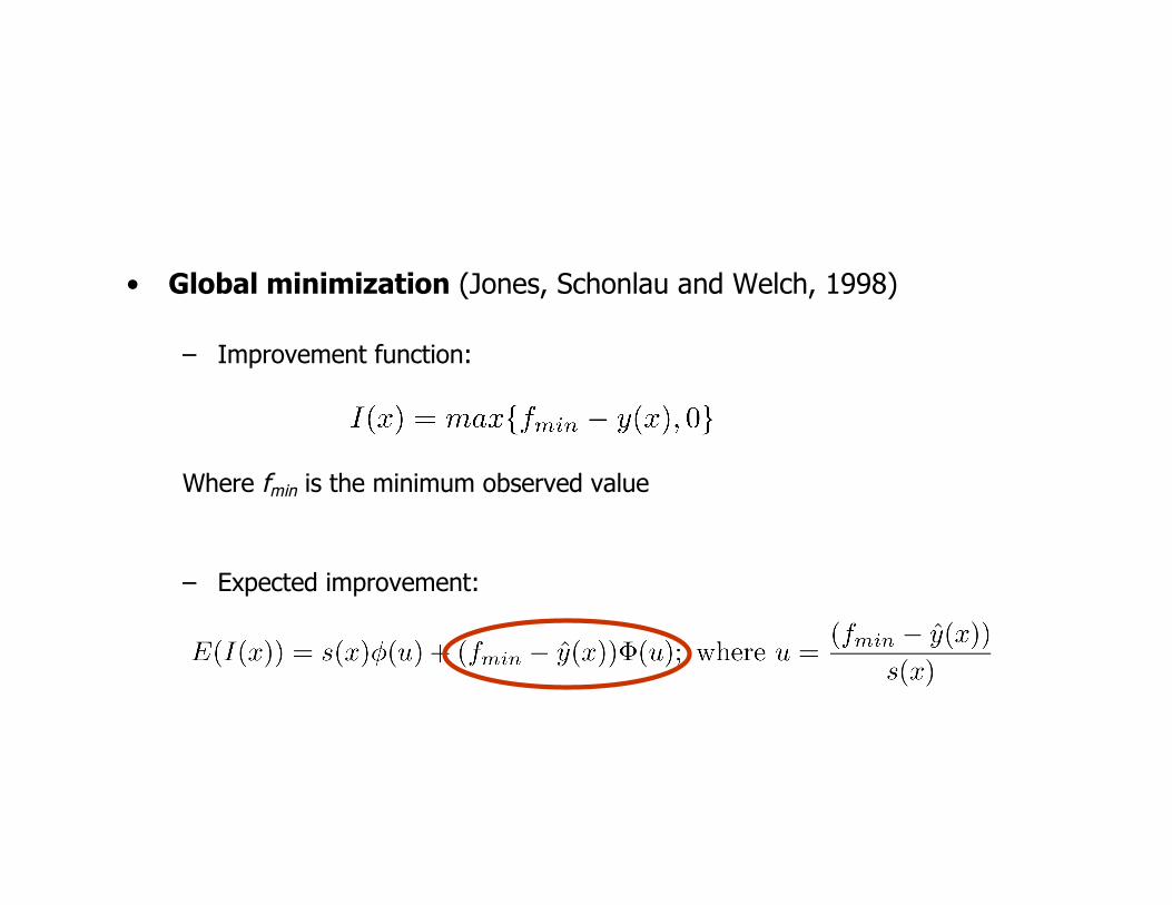
• Global minimization (Jones, Schonlau and Welch, 1998)

– Improvement function:

Where fmin is the minimum observed value

– Expected improvement:

Summary

• There are several expected improvement criteria for finding features of a response surface (quantiles, countours, optima, …)

• Idea is simple, strategy is the same

• Bingham et al., 2014 (arXiv:1601.05887)

Sample size

• So you want to run a computer experiment… why?

• For numerical integration, there are often bounds associated with the estimate of the mean (e.g., Koksma-Hlawka theorem … see Lemieux, 2009) derives an upper bound on the absolute integration error

• For computer model emulation Loeppky, Sacks and Welch (2009) proposed a general rule for n=10d

Sample sizeSimulation

• Suppose you have a realization of a GP in d-dimensions and also a hold-out set for validation

• Consider the impact of more active dimensions

• Efficiency index:

HOI =MSPE

ho

V ar(Yho

)

Sample size simulation

0

200

400

600 0

10

20

300

0.2

0.4

0.6

0.8

1

1.2

1.4

Active Dimensions

Multiplicative Gaussian Process

Run Size

Hold

Out

Inde

x

Sample size simulation… maybe it is not so bad after all

0100

200300

400500 0

510

1520

2530

0

0.2

0.4

0.6

0.8

1

1.2

1.4

Active Dimensions

Additive Gaussian Process

Run Size

Hold

Out

Inde

x