an intelligent alternating current-optimal power flow for

40

An intelligent alternating current-optimal power flow for reduction of pollutant gases with incorporation of variable generation resources

Sumant Lalljith1, Andrew G. Swanson1, Arman Goudarzi2* 1 School of Electrical, Electronics and Computer Engineering, University of KwaZulu-Natal, Howard College,

Durban 4001, South Africa. https://orcid.org/0000-0003-4798-7028 2 College of Electrical Engineering, Zhenjiang University, Hangzhou 310000, China; School of Electrical, Elec-

tronics and Computer Engineering, Mapua University, Manila, Philippines

ORCiDs: S. Lalljith: https://orcid.org/0000-0003-4798-7028 A.G. Swanson: https://orcid.org/0000-0002-9965-4746 A. Goudarzi: https://orcid.org/0000-0003-1264-6194

Abstract Frequent escalations in fuel costs, environmental concerns, and the depletion of non-renewable fuel reserves have driven the power industry to significant utilisation of renewable energy resources. These resources cannot satisfy the entire system load demand because of the intermittent nature of variable generation resources (VGRs) such as wind and solar. Therefore, there is a need to optimally schedule the generating units (thermal and VGRs) to reduce the amount of fuel used and the level of emissions produced. In this study, an AC-power flow in conjunction with combined economic and environmental dispatch approach through the implementa-tion of a modified constricted coefficient particle swarm optimisation was used to minimise the fuel cost and the level of emission gases produced. The approach was applied to the Institute of Electric and Electronic En-gineers 30 bus test system through three different load conditions: base-load, increase-load and critical-load. The results showed the practicality of the proposed approach for the simultaneous reduction of the total gen-eration cost and emission levels on a large electrical power grid while maintaining all the physical and opera-tional constraints of the system. Keywords: combined economic and emission dispatch, modified constricted coefficient particle swarm opti-misation, metaheuristic optimal power flow, variable generation resources

Highlights • Considering several physical and environmental constraints of generating units. • Proposing a metaheuristic method based on swarm intelligence for solving AC-OPF problem. • Incorporation of variable generation resources in electricity spot markets. • Maximisation of social welfare and minimisation of total generation cost, while reducing the volume of

pollutant gases.

Journal of Energy in Southern Africa 31(1): 40–61

DOI: https://dx.doi.org/10.17159/2413-3051/2020/v31i1a7008

Published by the Energy Research Centre, University of Cape Town ISSN: 2413-3051

This work is licensed under a Creative Commons Attribution-ShareAlike 4.0 International Licence

https://journals.assaf.org.za/jesa

Sponsored by the Department of Science and Technology

Corresponding author: Tel: 008613777894042; email: [email protected]

Volume 31 Number 1

February 2020

https://orcid.org/0000-0003-4798-7028

https://orcid.org/0000-0003-4798-7028

mailto:[email protected]

mailto:[email protected]

41 Journal of Energy in Southern Africa • Vol 31 No 1 • February 2020

1. Introduction

Optimal power flow (OPF) is the result of combin-ing economic dispatch (ED) and power flow studies [1]. The operating cost in ED is optimised by a suit-able distribution of the amount of power generated by different generating units. Its primary objective is to determine the optimal redistribution of the generator power outputs to meet the load demand at the minimum operating cost, while satisfying a set of qualitative system constraints. It has become necessary to not only minimise fuel cost but also re-duce the level of emissions gases, because of in-creased environmental concerns about thermal power plants releasing a significant level of pollu-tants such as mercury (𝐻𝑔0), carbon dioxide (𝐶𝑂2), sulphur oxides (𝑆𝑂𝑥) and nitrogen oxides (𝑁𝑂𝑥) into the atmosphere. The resulting problem is called combined economic and emission dispatch (CEED) [2]. Several methods to reduce the produc-tion of emission gases have been considered [2, 3]. The scheduling of generators, fuel cost and the transmission line characteristics of a power system network have a key influence over a generator’s ability to optimise the total production cost and transmission losses. System operators are required to schedule the generating units in a manner which lowers the rate of pollutant gas production. How-ever, this must be done together with maintaining the system security, especially in the presence of variable generation resources (VGRs).

Wind and solar power generation are the pri-mary categories of VGRs since they are very inter-mittent [3]. Solar power is a renewable energy, with sunlight converted into electrical energy using solar photovoltaic (PV) technology [3]. High capital costs and the need for appropriate geographical locations are becoming increasingly minor obstacles in the application of renewable energy resources because of a promising growth of the renewable energy re-search and development curve [3].

Traditionally, classical optimisation techniques like lambda iteration and linear programming were used to solve the optimal power flow (OPF) prob-lem with considerable accuracy and efficiency. However, optimisation, while maintaining an ac-ceptable system performance, renders it impracti-cal to solve the task using these traditional tech-niques [4]. There is an emerging need to integrate reliable artificial intelligence (AI) methods that can solve this complex problem efficiently. Heuristic AI optimisation methods, e.g., genetic algorithm, parti-cle swarm optimisation (PSO), and artificial bee col-ony are capable of handling complex system con-straints.

In this study, an OPF algorithm-based approach was used to reduce the level of emission gases pro-duced by conventional generators with respect to the global trend towards the reduction of pollution

gases. To solve the OPF problem, a modified me-taheuristic algorithm based on the improved ver-sion of PSO was designed.

2. Methodology

An algorithm was designed to utilise a larger pro-portion of intermittent renewable energy that is available at any one time. This was done with con-sideration to various real-world power system con-straints. Wind and solar PV generators were mod-elled for integration into the Institute of Electric and Electronic Engineers (IEEE) 30-bus test system. Af-ter a comprehensive study on different plausible heuristic AI optimisation techniques that could be used to efficiently solve the OPF problem, modified constricted coefficient particle swarm optimisation (MCCPSO) was developed. The following sub-sec-tions explain the formulated objective function and the proposed optimisation method.

Objective functions The OPF problem can be mathematically expressed as a series of equations starting with Equations 1 and 2.

Minimise 𝐹(𝑥) (1)

Subjected to 𝑔(𝑥) = 0 𝑎𝑛𝑑 ℎ(𝑥) ≤ 0 (2)

where 𝐹(𝑥) is the main objective function of the study; 𝑔(𝑥) represents the set of the equality con-straints; and ℎ(𝑥) defines the set of the inequality constraints.

Therefore, 𝑥𝑇 can be expressed as Equation 3 where 𝑛𝑔 is the number of the generator, 𝑃𝑔𝑛𝑔 is the active power of the generator 𝑛𝑔; 𝑉𝑔𝑛𝑔 is the voltage of the generator 𝑛𝑔; 𝑇𝑛𝑡 is the thermal limit of the transmission line 𝑛𝑡; and 𝑄𝑐𝑛𝑐 is the reactive power of the bus 𝑛𝑐.

𝑥𝑇 = [𝑃𝑔1, … 𝑃𝑔𝑛𝑔, 𝑉𝑔1, … 𝑉𝑔𝑛𝑔, 𝑇1, … 𝑇𝑛𝑡, 𝑄𝑐1, … 𝑄𝑐𝑛𝑐]

(3)

Economic dispatch objective function: The ED objective function is primarily used in the OPF problem for the minimisation of the overall cost of generation and is given by Equation 4.

𝐹𝐶 = ∑ (𝑎𝑖𝑃𝑔𝑖2 + 𝑏𝑖𝑃𝑔𝑖 + 𝑐𝑖);

𝑛𝑔

𝑖=1 𝑖𝑛 𝑈𝑆𝐷/ℎ (4)

where 𝐹𝐶 is the total generation cost function; 𝑎𝑖 , 𝑏𝑖 𝑎𝑛𝑑 𝑐𝑖 are the generators’ cost coefficients; and 𝑃𝑔𝑖 is the active power of the 𝑖𝑡ℎ generator.

Emission dispatch objective function: Pollu-tants such as 𝑆𝑂𝑥 and 𝑁𝑂𝑥 are major waste emis-sions into the atmosphere by thermal power plants.


The problem for minimising the quantity of emis-sions, 𝐸𝑇 , is formulated by including the reduction of emissions as an objective function using Equa-tion 5.

𝐸𝑇 = ∑ (𝑑𝑖𝑃𝑔𝑖2 + 𝑒𝑖𝑃𝑔𝑖 + 𝑓𝑖);

𝑛𝑔

𝑖=1𝑖𝑛 𝑘𝑔/ℎ (5)

where 𝐸𝑇 is the total generator emissions function and 𝑑𝑖 , 𝑒𝑖 𝑎𝑛𝑑 𝑓𝑖 are the generators’ emission coeffi-cients. The pollution control cost, 𝐹𝐸 (USD/h), can be obtained by assigning a cost factor to the pollu-tion level, expressed as in Equation 6.

𝐹𝐸 = ℎ𝑚𝐸𝑇; 𝑖𝑛 𝑈𝑆𝐷/ℎ (6)

where ℎ𝑚 is emission control cost factor and repre-sents the ratio of the maximum fuel cost to the min-imum emissions of the generating units [2], as in Equation 7.

ℎ𝑚 = ℎ𝑖1 + ((ℎ𝑖2 − ℎ𝑖1)

(𝑃𝑚𝑎𝑥2 − 𝑃𝑚𝑎𝑥1)) × (𝑃𝐷 − 𝑃𝑚𝑎𝑥1);

in USD/kg (7)

where ℎ𝑖2 𝑎𝑛𝑑 ℎ𝑖1 are price penalty factors associ-ated with the last and the current unit; 𝑃𝑚𝑎𝑥2 𝑎𝑛𝑑 𝑃𝑚𝑎𝑥1 are the maximum powers associ-ated with the last and the current unit; and 𝑃𝐷 is the power demand of the system. Therefore, the price penalty factor of the 𝑖𝑡ℎ unit (ℎ𝑖) can be calculated using Equation 8.

ℎ𝑖 = 𝐹𝑐𝑖(𝑃𝑔𝑖

𝑚𝑎𝑥)

𝐸𝑇𝑖(𝑃𝑔𝑖𝑚𝑎𝑥)

; 𝑖𝑛𝑈𝑆𝐷

𝑘𝑔 (8)

where 𝐹𝑐𝑖 is the generation cost of the 𝑖𝑡ℎ unit and 𝐸𝑇𝑖 is the emission volume of the 𝑖𝑡ℎ unit.

The CEED objective function: The ED mini-mises the total operating cost at the expense of in-creasing the rate of emission gases such as 𝑁𝑂𝑥 . On the contrary, emission dispatch minimises the vol-ume of emission gases released by the system at the expense of an increased system operating cost. In this study, the operating and emission cost simulta-neously was reduced mathematically as in Equation 9.

Minimise 𝑓(𝐹𝐶 , 𝐹𝐸) (9)

subject to the load demand equality and the gener-ator inequality constraints.

A multi-dimensional optimisation is converted into a single-dimensional optimisation problem by introducing the price penalty factor, ℎ𝑚, in Equation 10.

𝐹𝑇 = ∑((𝑎𝑖𝑃𝑔𝑖

2 + 𝑏𝑖𝑃𝑔𝑖 + 𝑐𝑖) +

ℎ𝑚(𝑑𝑖𝑃𝑔𝑖2 + 𝑒𝑖𝑃𝑔𝑖 + 𝑓𝑖)

)

𝑛𝑔

𝑖=1

;

𝑖𝑛 𝑈𝑆𝐷/ℎ (10)

The equality constraints: The 𝑖𝑡ℎ bus injected active and reactive powers are described using equality constraints and can be defined by Equation 11 [5].

∑ 𝑃𝑔𝑖𝑛𝑔𝑗=1 = 𝑃𝐷 + 𝑃𝑙𝑜𝑠𝑠𝑒𝑠 ; 𝑖𝑛 𝑀𝑊 (11)

where 𝑃𝑙𝑜𝑠𝑠𝑒𝑠 is the total generation loss. The inequality constraints: The inequality

constraints associated with the power system net-work represent the physical limits of the compo-nents. These constraints ensure maintenance of the system security [5]. Equations 12–15 represent the inequality constraints of the control variables con-sidered in this study.

(i) Active power generation constraint at the generator buses

𝑃𝑔𝑖,𝑚𝑖𝑛 ≤ 𝑃𝑔𝑖 ≤ 𝑃𝑔𝑖,𝑚𝑎𝑥 (12)

(ii) Reactive power generation constraint at the generator buses

𝑄𝑔𝑖,𝑚𝑖𝑛 ≤ 𝑄𝑔𝑖 ≤ 𝑄𝑔𝑖,𝑚𝑎𝑥 (13)

(iii) Transmission line power flow constraint

𝑀𝑉𝐴𝑓𝑝,𝑞 ≤ 𝑀𝑉𝐴𝑓𝑝,𝑞𝑚𝑎𝑥 (14)

(iv) The voltage of each P-Q bus constraint

𝑉𝑖,𝑚𝑖𝑛 ≤ 𝑉𝑖 ≤ 𝑉𝑖,𝑚𝑎𝑥 (15)

where 𝑃𝑔𝑖,𝑚𝑖𝑛 𝑎𝑛𝑑 𝑃𝑔𝑖,𝑚𝑎𝑥 are the minimum and

the maximum active generation capacity of the 𝑖𝑡ℎ generator; 𝑄𝑔𝑖,𝑚𝑖𝑛 𝑎𝑛𝑑 𝑄𝑔𝑖,𝑚𝑎𝑥 are the minimum

reactive generation capacity of the 𝑖𝑡ℎ generator; 𝑀𝑉𝐴𝑓𝑝,𝑞 is the transmission line power flow con-

straint between bus 𝑞 and bus 𝑝; 𝑀𝑉𝐴𝑓𝑝,𝑞𝑚𝑎𝑥 is the

maximum power that can flow between bus 𝑞 and bus 𝑝; and 𝑉𝑖,𝑚𝑖𝑛 𝑎𝑛𝑑 𝑉𝑖,𝑚𝑎𝑥 are the minimum and

the maximum voltage of the 𝑖𝑡ℎ P-Q bus constraint.

2.2 Variable generation resources Wind power generation: The wind speed gained by the wind turbines is usually effective at 50–100 m above ground [6]. Thus, the wind speed meas-ured by the anemometer (at its height above ground) needs to be converted to the turbine’s hub height [7]. Equation 16 explains the relationship of the wind speeds at different height hubs.

𝑣2

𝑣1= (

ℎ2

ℎ1)𝛼

(16)


where 𝑣1 𝑎𝑛𝑑 𝑣2 are the wind speed at the initial and the changed hub height respectively; ℎ1 𝑎𝑛𝑑 ℎ2 are the hub height of the initial and selected point respectively; and 𝛼 is the friction coefficient that implicates actual parameters such as the roughness of terrain and temperature. The power generated from the wind turbine can be approximated by Equation 17 [7] (see foot of page).

The cost of wind power generation: The total cost of power production from the wind farm can be calculated using Equation 18 [8, 9] (see foot of page).

The solar PV power generation: Solar PV power is reliant on natural occurrences such as so-lar irradiance and the ambient temperature. These quantities are directly related to geographical loca-tion and season. The power generated from a solar PV farm is calculated by Equation 19 [10, 11].

𝑃𝑜(𝑠) = 𝑁 × 𝐹𝐹 × 𝑉𝑃𝑉 × 𝐼𝑃𝑉 ; 𝑖𝑛 𝑊 (19)

For a given radiation level and ambient temper-ature, the voltage-current characteristics of a PV module are determined using Equations 20–23.

𝐹𝐹 = 𝑉𝑀𝑃𝑃𝑇 × 𝐼𝑀𝑃𝑃𝑇𝑉𝑂𝐶 × 𝐼𝑆𝐶

(20)

𝑇𝑃𝑉 = 𝑇𝐴 − 𝑠 (𝑁𝑂𝑇 − 20

0.8) ; 𝑖𝑛 ℃ (21)

𝐼𝑃𝑉 = 𝑠[𝐼𝑆𝐶 + 𝐾𝑖(𝑇𝑃𝑉 − 25)]; 𝑖𝑛 𝐴 (22)

𝑉𝑃𝑉 = 𝑉𝑂𝐶 − 𝐾𝑣 × 𝑇𝑃𝑉 ; 𝑖𝑛 𝑉 (23)

where 𝑃𝑜(𝑠) is the power generated by the solar farm; 𝑠 is the solar irradiance; 𝑁 is the number of the PV modules; 𝐹𝐹 is the fill factor of the PV mod-ule; 𝑉𝑃𝑉 is the voltage of the PV module; 𝐼𝑃𝑉 is the current of the PV module; 𝑉𝑀𝑃𝑃𝑇 is the voltage of the maximum power point tracking of the PV module; 𝐼𝑀𝑃𝑃𝑇 is the current of the maximum power point tracking of the PV module; 𝑉𝑂𝐶 is the open-circuit voltage of the PV module; 𝐼𝑆𝐶 is the short-circuit cur-rent of the PV module; 𝐾𝑣 is the voltage tempera-ture coefficient; 𝑇𝑃𝑉 is the PV cell temperature; 𝐾𝑖 is the current temperature coefficient; and 𝑉𝑂𝐶 is the open-circuit voltage.

The cost of solar PV generation: The total cost of power production from the solar PV farm can be calculated using a cost function represented by Equation 24 [12] (see foot of page).

The penalty cost coefficient is caused by not us-ing all the available wind/solar PV power available. It is the difference between the available wind power and the actual wind power used. The reserve cost coefficient is caused by under-generation; hence this coefficient is associated with the calling of reserves for compensation [9]

𝑃𝑤𝑖𝑛𝑑 =

{

0

𝑉3

𝑃𝑟

(𝑃𝑟

𝑉𝑟3 − 𝑉𝑐𝑢𝑡−𝑖𝑛

3 ) − 𝑃𝑟 (𝑉𝑐𝑢𝑡−𝑖𝑛3

𝑉𝑟3 − 𝑉𝑐𝑢𝑡−𝑖𝑛

3 )

; 𝑉 < 𝑉𝑐𝑢𝑡−𝑖𝑛 , 𝑉 > 𝑉𝑐𝑢𝑡−𝑜𝑢𝑡

; 𝑉𝑐𝑢𝑡−𝑖𝑛 ≤ 𝑉 < 𝑉𝑟

; 𝑉𝑟 ≤ 𝑉 ≤ 𝑉𝑐𝑢𝑡−𝑜𝑢𝑡

(17)

where 𝑃𝑤𝑖𝑛𝑑 is the power generated by the wind turbine; 𝑉 is the wind speed, 𝑉𝑐𝑢𝑡−𝑖𝑛 is the cut-in wind speed of the wind turbine; 𝑉𝑐𝑢𝑡−𝑜𝑢𝑡 is the cut-out speed of the wind turbine; 𝑉𝑟 is the rated speed of the wind turbine; and 𝑃𝑟 is the rated power wind turbine.

𝐶𝑤𝑖 = ∑ 𝑑𝑖(𝑤𝑖) +𝑁𝑊𝑖=1 ∑ 𝑘𝑝.𝑖(𝑤𝑖) +

𝑁𝑊

𝑖=1∑ 𝑘𝑟.𝑖(𝑤𝑖)𝑁𝑤𝑖=1 ; in USD/h (18)

where 𝐶𝑤𝑖 is the total cost of the generated power by the 𝑖𝑡ℎ wind farm; 𝑤𝑖 is the total generated power by the 𝑖𝑡ℎ wind farm; 𝑑𝑖(𝑤𝑖) is the direct cost of wind power; 𝑘𝑝.𝑖(𝑤𝑖) is the penalty cost coefficient for overes-timation of the wind power; and 𝑘𝑟.𝑖(𝑤𝑖) is the reserve cost for the underestimation of the wind power.

𝐶𝑆𝑖 = ∑ 𝑑𝑖(𝑆𝑖) +𝑁𝑃𝑉𝑖=1 ∑ 𝑘𝑝.𝑖(𝑆𝑖) +

𝑁𝑃𝑉

𝑖=1∑ 𝑘𝑟.𝑖(𝑆𝑖)𝑁𝑃𝑉𝑖=1 ; in USD/h (24)

where 𝐶𝑆𝑖 is the total cost of the generated power by the 𝑖𝑡ℎ solar farm, 𝑆𝑖 is the total generated power by the 𝑖𝑡ℎ solar farm, 𝑑𝑖(𝑆𝑖) is the direct cost of solar power, 𝑘𝑝.𝑖(𝑆𝑖) is the penalty cost coefficient for overesti-mation of the solar power; and 𝑘𝑟.𝑖(𝑆𝑖) is the reserve cost for the underestimation of the solar power.


2.3 Formulation of the MCCPSO-OPF Load flow methodology: In an electrical grid, power flows from the generation stations to the load centres. Thus, an investigation is required to determine the bus voltages and the power flow through the transmission lines. There are many methods (such as Newton-Raphson (NR), Gauss-Siedel, or Fast-Decoupled [13]) that can be used to perform the load flow calculations, however, to en-sure that the system performs at an optimal level a load flow method needs to be selected based on merit and practicality. The NR method was selected because of its mathematical superiority and accu-racy [14–17].

2.4 A modified constriction coefficient PSO The PSO is a population-based stochastic optimisa-tion technique developed in 1995 and inspired by the social behaviour of birds flocking and fish schooling [18]. In other words, its development was based on the behavioural ability of the swarms to share their information with each other (infor-mation is what food sources, danger, etc, are re-ferred to as), where this characteristic increases the efficiency of the entire swarms as opposed to indi-vidual particle exploration.

The PSO contains a population of candidate so-lutions (randomly generated on the first iteration) called a swarm. In every iteration, every particle is a candidate solution to the optimisation problem, in which every particle has a position in the search space. Consider the particle having a position and velocity as stated in Equations 25 and 26.

For particle 𝑖,

• Position:

𝑥𝑖⃑⃑ ⃑(𝑡) ∈ 𝑋 (25)

• Velocity:

𝑣𝑖⃑⃑⃑ (𝑡) ∈ 𝑋 (26)

Figure 1 shows a simple model of a moving par-ticle in PSO, one which is not alone but part of a swarm. A particle (𝑥𝑙(𝑡)) moves towards the opti-

mum solution based on its present velocity (𝑣𝑙(𝑡)), its previous experience (stored in memory) and the experience of its neighbours. In addition to the po-

sition and velocity of the particle, every particle has a memory of its own best position. This is denoted by 𝑃𝑖⃑⃑ (𝑡), which represents the personal best experi-

ence of the particle. In addition to 𝑃𝑖⃑⃑ (𝑡), there is a common best experience among the members of the swarm. This is denoted by 𝐺(𝑡) (this is not de-

noted by 𝑖, as it belongs to the entire swarm and not just to the particle), which represents the global best experience of all the particles in the swarm.

The mathematical model of PSO is simple. By de-fining these concepts on every iteration of PSO the position and velocity of the particle are updated ac-

cording to the best experience. Figure 1 defines a vector from the current position to the personal best solution and a vector from the current position

to the global best. The particle tends to move to-wards the new position using all the vectors shown. The black line indicates the motion of the vector as

it moves to the new position (denoted by 𝑥𝑖⃑⃑⃑ (𝑡 + 1) ). The new velocity is denoted by 𝑣𝑖⃑⃑⃑ (𝑡 + 1). A new position is created according to the previous veloc-

ity 𝑣𝑖⃑⃑⃑⃑ (𝑡), the personal best 𝑃𝑖⃑⃑ (𝑡), and the global best 𝐺(𝑡). Therefore, 𝑥𝑖⃑⃑⃑ (𝑡 + 1) is probably a better loca-tion (solution) as the particle was guided by its own

motion (its memory of the previous best experience and the experience of the entire swarm). The veloc-ity and position of each particle can be calculated

using Equations 27 and 28 (see top of next page). In the velocity updating process, the values of

parameters such as 𝑐1 and 𝑐2 are equal to 2.05. The

𝑟1 and 𝑟2 generate random numbers between 0 and 1. Equations 26 and 27 represent the basic version

Figure 1: Geometric representation of a particle in particle swarm optimisation [1].


𝑣𝑖⃑⃑⃑ (𝑡 + 1) = 𝑣𝑖⃑⃑⃑ (𝑡)⏟ +𝑐𝑢𝑟𝑟𝑒𝑛𝑡 𝑚𝑜𝑡𝑖𝑜𝑛

𝑐1. 𝑟1. (𝑃𝑖⃑⃑ (𝑡) − 𝑥𝑖⃑⃑⃑ (𝑡))⏟ 𝑝𝑎𝑟𝑡𝑖𝑐𝑙𝑒 𝑚𝑒𝑚𝑜𝑟𝑦

+ 𝑐2. 𝑟2. (𝐺(𝑡) − 𝑥𝑖⃑⃑⃑ (𝑡))⏟ 𝑠𝑤𝑎𝑟𝑚 𝑖𝑛𝑓𝑙𝑢𝑒𝑛𝑐𝑒

(27)

𝑥𝑖⃑⃑⃑ (𝑡 + 1) = 𝑥𝑖⃑⃑⃑ (𝑡) + 𝑣𝑖⃑⃑⃑ (𝑡) (28)

𝑣𝑖⃑⃑⃑ (𝑡 + 1) = 𝑣𝑖⃑⃑⃑ (𝑡)⏟ +𝑐𝑢𝑟𝑟𝑒𝑛𝑡 𝑚𝑜𝑡𝑖𝑜𝑛

𝑐1. (1 − 𝑟1(𝑉𝑎𝑟𝑠𝑖𝑧𝑒)) . (𝑃𝑖⃑⃑ (𝑡) − 𝑥𝑖⃑⃑⃑ (𝑡))⏟ 𝑝𝑎𝑟𝑡𝑖𝑐𝑙𝑒 𝑚𝑒𝑚𝑜𝑟𝑦

+ 𝑐2. (1 − 𝑟2(𝑉𝑎𝑟𝑠𝑖𝑧𝑒)). (𝐺(𝑡) − 𝑥𝑖⃑⃑⃑ (𝑡))⏟ 𝑠𝑤𝑎𝑟𝑚 𝑖𝑛𝑓𝑙𝑢𝑒𝑛𝑐𝑒

(29)

of the PSO algorithm, but several modifications are necessary to enhance the performance of the PSO.

Thus, this study has proposed the following methods to modify the basic PSO:

Modification #1: In order to enhance the func-tionality of the random components’ coefficients of the vector of velocity (𝑟1 and 𝑟2), they should gener-ate the random numbers according to the size of the variable matrix and the produced values should be subtracted from 1. Therefore, Equation 27 can be modified as Equation 29 (see top of page)

Modification #2: The vector of velocity should go under a refinement process once its values are defined through the Equation 29, to further improve its performance, as shown in Equations 30 and 31.

𝑣𝑖⃑⃑⃑ (𝑡 + 1) = 𝑠𝑔𝑛(𝑣𝑖⃑⃑⃑ (𝑡 + 1)) + min[|𝑣𝑖⃑⃑⃑ (𝑡 + 1)|, 𝑉𝑒𝑙𝑚𝑎𝑥],

(30) where

𝑉𝑒𝑙𝑚𝑎𝑥 = 0.5 × (𝑉𝑎𝑟𝑚𝑎𝑥 − 𝑉𝑎𝑟𝑚𝑖𝑛), (31)

where 𝑉𝑒𝑙𝑚𝑎𝑥 is the maximum range of the vector of the velocity at that step; and 𝑉𝑎𝑟𝑚𝑎𝑥𝑎𝑛𝑑 𝑉𝑎𝑟𝑚𝑖𝑛 are the maximum and minimum values for the size of the variables.

Modification #3: In this formulation, the study has implemented a constriction coefficient method to precisely determine the values of the velocity co-efficient (𝑐1 and 𝑐2). The amplitude of a particle os-cillations decreases as it focuses on the local and

neighbourhood previous best positions. Through this method, the movement of particles will be con-fined to optimum point over time, also it prevents the particles from trapping in local minima [17]. The third modification for improving the perfor-mance of PSO can be implemented through Equa-tions 32–35.

𝜒 =2.𝑘

|2−𝜑−√𝜑2−4𝜑|

(32)

𝜑 = 𝜑1 + 𝜑2 ≥ 4.1 (33)

𝑐1 = 𝜒𝜑1 (34)

𝑐2 = 𝜒𝜑2 (35) where 𝜒 is the constriction coefficient; 𝑘 is the con-stant multiplier in the constriction coefficient tech-nique (typically, the value of 𝑘 is between 0.73 to 1); 𝜑 is the convergence factor; 𝑐1 is the fixed coeffi-cient for the personal best experience and 𝑐2 is the fixed coefficient for the global best experience.

Modification #4: To create a suitable balance between the exploration and exploitation during the optimisation process, the study proposed a non-linear time-varying damping inertia (NLTVD) tech-nique. The NLTVD dynamically reduces the value of damping inertia from its maximum value towards its lower bound as the optimisation progresses. Also, it prevents the PSO from any premature con-vergence. (See Equations 36 and 37 below.)

𝑊𝐷𝑎𝑚𝑝 = 𝑊𝑀𝑎𝑥 × [(𝑊𝑀𝑎𝑥 −𝑊𝑀𝑖𝑛 − 𝛼1) exp (

1

1+ 𝛼2×𝐼𝑡𝑒𝑟𝑖

𝑀𝑎𝑥𝐼𝑡𝑒𝑟

)] (36)

𝑣𝑖⃑⃑⃑ (𝑡 + 1) = 𝑊𝐷𝑎𝑚𝑝 . 𝑣𝑖⃑⃑⃑ (𝑡)⏟ +

𝑐𝑢𝑟𝑟𝑒𝑛𝑡 𝑚𝑜𝑡𝑖𝑜𝑛

𝑐1. (1 − 𝑟1(𝑉𝑎𝑟𝑠𝑖𝑧𝑒)). (𝑃𝑖⃑⃑ (𝑡) − 𝑥𝑖⃑⃑⃑ (𝑡))⏟ 𝑝𝑎𝑟𝑡𝑖𝑐𝑙𝑒 𝑚𝑒𝑚𝑜𝑟𝑦

+

𝑐2. (1 − 𝑟2(𝑉𝑎𝑟𝑠𝑖𝑧𝑒)). (𝐺(𝑡) − 𝑥𝑖⃑⃑⃑ (𝑡))⏟ 𝑠𝑤𝑎𝑟𝑚 𝑖𝑛𝑓𝑙𝑢𝑒𝑛𝑐𝑒

,

(37)

where 𝑊𝑀𝑎𝑥 𝑎𝑛𝑑 𝑊𝑀𝑖𝑛 are the maximum (0.9) and minimum (0.4) values for the damping inertia coeffi-cient; 𝛼1 and 𝛼2 are multiplicative coefficients of NLTVD, where the value of 𝛼1 is 0.2 and the value of 𝛼2 is 7; 𝐼𝑡𝑒𝑟𝑖 is the current iteration; and 𝑀𝑎𝑥𝐼𝑡𝑒𝑟 is the maximum number of iterations.


𝑥𝑖⃑⃑⃑ (𝑡 + 1) = {𝑥𝑖⃑⃑⃑ (𝑡 + 1) 𝑖𝑓 𝑟𝑎𝑛𝑑𝑖(𝑃𝑜𝑝𝑛𝑢𝑚𝑏𝑒𝑟 , 𝑉𝑎𝑟𝑠𝑖𝑧𝑒) ≤ 0.75

𝑃𝑖⃑⃑ (𝑡) 𝑂𝑡ℎ𝑒𝑟𝑤𝑖𝑠𝑒 , (38)

where 𝑃𝑜𝑝𝑛𝑢𝑚𝑏𝑒𝑟 is the population number; and 𝑟𝑎𝑛𝑑𝑖 generates random integers according to population number and size of the variables.

Modification #5: To reduce the destructive im-

pact of the weak particles, a crossover operator is implemented. The proposed crossover operator di-versifies the populations in each iteration and it avoids the re-exploration of the inappropriate zones. (See Equation 38 at top of page.)

2.5 System overview Application of MCCPSO in OPF: Using Equation 10, the objective function implemented in MCCPSO is defined in Equation 39.

∑𝐹𝑇(𝑃𝑔𝑖)

𝑛𝑔

𝑖=1

+ 100. 𝑎𝑏𝑠 (∑𝑃𝑔𝑖 − 𝑃𝐷 −

𝑛𝑔

𝑖=1

𝑃𝑙𝑜𝑠𝑠𝑒𝑠) ;

𝑖𝑛 𝑈𝑆𝐷/ℎ (39)

Therefore, the constrained optimisation prob-lem is converted into an unconstrained problem us-ing the price penalty factor method (Equation 8). The MCCPSO algorithm in Equation 39 deals di-rectly with the real power constraint. The applica-tion of the MCCPSO algorithm is shown in Figure 2.

Figure 2: Flow chart representing the application of modified constriction coefficient particle swarm

optimisation in solving the optimal power flow problem (𝒂𝒊, 𝒃𝒊, 𝒄𝒊, 𝒅𝒊, 𝒆𝒊, 𝒇𝒊 are the generators cost and

emission coefficients; 𝑷𝑫 is the total load demand; 𝑰𝒕𝒆𝒓 is the current iteration; 𝑴𝒂𝒙𝑰𝒕𝒆𝒓 is the

maximum iteration, �⃑⃑� 𝒍(𝒕) is the personal best; �⃑⃑� (𝒕) is the global best; �⃑⃑� 𝒍(𝒕) is the updated vector

velocity; �⃑⃑� 𝒍(𝒕) is the updated vector of positions; 𝑭𝑻𝒃𝒆𝒔𝒕 is the best fitness function; and 𝑭𝑻

𝒏𝒆𝒘 is the

new fitness function).


Figure 3: Flow chart showing the Newton-Raphson interface with modified constriction coefficient particle swarm optimisation (CEED represents the combined environmental economic dispatch).

After the MCCPSO algorithm determined the

global optimum solution for the CEED objective function, the line-flow power in megavolt amperes (MVA) was calculated for the entire network. If the calculated line-flow power (MVA) exceeded the rated line-flow MVA, then the algorithm selects the previous 𝐺(𝑡) value as the global optimum solution to the problem. This procedure prevents the trans-mission lines from being overloaded.

Newton-Raphson power flow solution: The test system data is taken from Sadaat [13]. The bus data (admittance bus, denoted by 𝑌𝑏𝑢𝑠) is used to obtain the load flow solution for the intelligent AC-OPF. The MCCPSO-OPF updates the generated power column of the bus data matrix, which indi-cates the power required to be generated by each generator in the system. The losses in the system are calculated only at the end of the iteration. The difference in power injection and power demand is the loss of the system. This extra power must be ac-commodated in the load flow for the next iteration. Hence the slack bus, being the generator bus with the highest generating capacity, accepts this extra burden to balance the system. Therefore, at this bus, the voltage magnitude and phase angle are speci-fied, and the real and reactive powers are calcu-lated. Figure 3 depicts the process of power flow analysis with the help of MCCPSO.

Wind power model: Three wind farms will be integrated into the IEEE 30-bus network and are modelled with respect to wind farm projects in South Africa [20] as indicated in Table 1. The total

installed capacity of these wind farms was 56.7 MW. By means of the input parameters presented in Ta-ble 1, it was possible to model the wind farms for this study using Equations 18 and 19. For the best practical results, using the average wind speed data (approximately 7 m/s) gathered from the actual wind farm locations [24], an artificial wind speed simulator was developed in MATLAB R2018a.

Solar PV power model: For the integration of solar PV energy into this study, a 10 MW PV gener-ator was considered. Solar irradiance and the ambi-ent temperature data collected by the University of KwaZulu-Natal [25] was utilised for this model. Ta-ble 2 indicates the solar panel parameters. Follow-ing the design of a 5 MW solar PV farm [26], which used 22560 PV modules to produce this output power capacity, it takes 45 455 solar PV modules to produce 10 MW.

System integration: Considering the single-line diagram of the IEEE 30-bus network in Sadaat [13], the cookhouse, Gouda and Enel’s Gibson Bay wind farms were strategically placed at buses 30, 29, and 24 respectively. The solar PV farm (10 MW) was placed at bus 23. Figure 4 illustrates a simple sche-matic of the overall power system network after in-tegration.

One of the main objectives of this study was to create a control system that intelligently utilises a larger proportion of variable renewable energy when available to supply the load demand. The MCCPSO algorithm was designed to carry out this operation. The system algorithm first considered


Table 1: Wind power model input parameters.

Parameters Unit

Name of wind farm

Cookhouse wind farm

Gouda wind farm Enels Gibson Bay wind farm

Turbine model Suzlon S88 [21] AW3000 [22] Nordex N117 [23]

Blades diameter m 1.390 2.217 1.578

Swept area m2 6.082 15.431 7.823

Efficiency % 0.95 0.95 0.97

Reference height, ℎ1 m 43.6 43.6 42.0

Hub height, ℎ2 m 80 82 100

Cut-in speed, 𝑉𝑐𝑢𝑡−𝑖𝑛 m/s 4.0 3.0 3.5

Rated speed, 𝑉𝑟 m/s 14 10 12

Cut-out speed, 𝑉𝑐𝑢𝑡𝑜𝑢𝑡 m/s 25 20 25

No. of turbine units 12 5 5

Rated power, 𝑃𝑟 MW 2.1 3.0 3.3

Wind farm total power capacity

MW 25.2 15.0 16.5

Lifetime (years) 24 24 24

Table 2: Mono-crystalline solar panel parameters.

Parameter Value Unit

Nominal capacity 220 W

Number of PV modules 45455

Maximum power point voltage, 𝑉𝑀𝑃𝑃𝑇 28.36 V

Maximum power point current, 𝐼𝑀𝑃𝑃𝑇 7.76 A

Open circuit voltage, 𝑉𝑂𝐶 36.96 V

Short circuit current, 𝐼𝑆𝐶 8.36 A

Nominal operating temperature, 𝑁𝑂𝑇 43 ℃

Ambient temperature coefficient, 𝑇𝐴 30.76 ℃

Voltage temperature coefficient, 𝐾𝑣 0.1278 V/℃

Current temperature coefficient, 𝐾𝑖 0.00545 A/℃

the amount of renewable power available at each hour to supply the load demand, the remainder of the load demand was then allocated to the conven-tional generators in the system. Equation 40 defines this operation.

𝑃𝐷𝑁𝑒𝑤 = 𝑃𝐷 − (𝑃𝑆 + 𝑃𝑊) 𝑖𝑛 𝑀𝑊 (40)

where 𝑃𝐷𝑁𝑒𝑤 is the new load demand of the system;

𝑃𝑆 is total generated power by the solar farm; and 𝑃𝑊 is the total generated power by the wind farm.

3. Results and discussion

The system designed and simulated on MATLAB was executed on Inter ® CoreTM i5-7200U (2.7 GHz), 4.00 GB RAM (DDR5) and windows 10 OS

(personal property). First, this section defines the main contributions of this study:

i) The proposed MCCPSO was employed to solve the OPF problem using the CEED objective func-tion.

ii) Three wind farms were modelled on the basis of a novel algorithm formulated to artificially con-vert the generated wind speed variations to the power output of WTGs. iii) A novel mathematical formulation was proposed to model the power output of mono-crystalline PV-arrays.

iv) The proposed MCCPSO algorithm was imple-mented to intelligently utilise a large proportion of VGRs to meet the load demand at the specified hour.


Figure 4: Simple schematic of the integrated hybrid power system network.

v) A proposed metaheuristic OPF approach was able to maximise the social welfare, while mini-mise the volume of the produced pollutant gases.

3.1 The MCCPSO-OPF on the Original IEEE 30-bus The original IEEE 30-bus test network specifica-tions are shown in Table 3 [27, 28].

Table 3: IEEE 30-bus system.

IEE

E 3

0-b

us

net

wo

rk

spec

ific

ati

on

s

Slack bus 1

Regulated buses (con-ventional generators)

2, 5, 8, 11 and 13

Load buses (remaining buses)

Load demand 283.4 MW

Fuel cost 901.59 USD/h

Rate of emission gases produced

470 kg/h

Table 4 indicates the resultant IEEE 30-bus fuel

cost after applying the MCCPSO algorithm through ED and presents the potential of the proposed AI al-gorithm by comparing it with other AI optimisation algorithms under similar circumstances.

Table 5 indicates the new rate of emission gases produced through MCCPSO-OPF using the different objective functions. Although the level of emissions produced is slightly higher than what was achieved through emission dispatch, the total cost of produc-tion is significantly less; thus, an appropriate bal-ance between the fuel cost and the level of emission

gases has been established. Considering the initial fuel cost and rate of emission gases emitted, through the proposed CEED function there were 7.67% and 27% reductions in 𝑈𝑆𝐷/ℎ and 𝑘𝑔/ℎ re-spectively. This remarkable outcome can be at-tributed to the fact that dispatching the cheapest generators in a power system to meet the load de-mand cannot guarantee the optimum cost of opera-tion as it can increase the power losses with respect to the geographical location of the generators and loads. The total cost of generation and the emis-sions released by each generating unit are shown respectively in Figures 5 and 6.

Use of the CEED objective function resulted in the dispatched power being more economical than the ED objective function, which overburdened the slack bus to optimise the fuel cost as depicted in Fig-ure 5. Overloading of the slack bus to minimise the fuel cost resulted in a significant increase in the rate of emissions released by the slack bus alone, affect-ing the overall cost of production as shown in Fig-ure 5. Overloading of the slack bus is a common is-sue in economic load dispatch, however, several methods to distribute this burden were studied by Panda [29].

3.2 Wind generator model The wind speed generator was simulated to inves-tigate the severe restrictions of the wind turbine for each wind farm. Figure 6 shows the wind speed characteristics at the selected wind farms. Figure 7 shows the power generated by each wind farm and the combined generated power. The model was de-veloped over 12 hours, but was extended to 24 hours


Table 4: Comparison of AI results based on the IEEE 30-bus (𝑷𝒈𝒊,𝒎𝒊𝒏 and 𝑷𝒈𝒊,𝒎𝒂𝒙 are the minimum and

maximum generation limits of the generators; ABC is the artificial bee colony algorithm; GA is the genetic algorithm; and MCCPSO is modified constriction coefficient particle swarm optimisation).

Generator unit (MW)

𝑃𝑔𝑖,𝑚𝑖𝑛 𝑃𝑔𝑖,𝑚𝑎𝑥 ABC method [15] GA method [15] Proposed MCCPSO method

P1 (bus 1) 50 200 173.826 176.026 176.6988

P2 (bus 2) 20 80 48.998 49.453 48.8208

P3 (bus 5) 15 50 21.386 20.737 21.3942

P4 (bus 8) 10 35 22.63 21.517 21.9478

P5 (bus 11) 10 30 12.928 12.699 11.9130

P6 (bus 13) 12 40 12.00 12.445 12.0000

Fuel cost (USD/h) 802.557 802.328 801.844

Table 5: MCCPSO-OPF using different objective functions (𝑷𝒈𝒊,𝒎𝒊𝒏 and 𝑷𝒈𝒊,𝒎𝒂𝒙 are the minimum and

maximum generation limits of the generators; CEED is the combined environmental economic dispatch).

Generator unit (MW) 𝑃𝑔𝑖,𝑚𝑖𝑛 𝑃𝑔𝑖,𝑚𝑎𝑥 Economic dispatch

𝑓(𝐹𝐶)

Emission dispatch

𝑓(𝐹𝐸)

Proposed CEED

𝑓(𝐹𝐶 , 𝐹𝐸)

P1 (bus 1) 50 200 176.6988 112.3772 123.5956

P2 (bus 2) 20 80 48.8208 47.0000 49.1435

P3 (bus 5) 15 50 21.3942 34.7692 29.0937

P4 (bus 8) 10 35 21.9478 31.3926 31.5048

P5 (bus 11) 10 30 11.9130 30.0000 27.5048

P6 (bus 13) 12 40 12.0000 33.1078 28.1950

Power loss NA NA 9.3746 5.2468 5.9436

Fuel cost (USD/h) NA NA 801.8456 852.7765 832.4083

Emission (kg/h) NA NA 424.4792 340.0032 343.6777

Total cost (USD/h) NA NA 1791.052 1645.120 1633.314

Figure 5: Generator statistics for the combined environmental economic dispatch problem.


Figure 6: Generated wind speeds at each farm.

Figure 7: Wind power generation model.

when integrated. The energy produced by wind farms was directly proportional to wind speed var-iations. The total cost of wind power generation for each hour is also indicated in Figure 7.

3.3 Solar PV generator model In general, the temperature and irradiance levels peak between 11:00 and 15:00 pm when the sun’s intensity is brightest, hence maximum power out-put can be expected from the PV farm during this period. The amount of solar irradiance present di-rectly affects the amount of power produced by the 10 MW farm, as shown in Figure 8.

On every execution of the PV model over 24 hours, the results produced are dependent on the sample of seasonal data collected from [25]. As the amount of power generated by the PV model increases,

so does the cost of production (USD/h). The model generally produced the best distribution of power output during the day in summer (based on an av-erage summer day).

3.4 Generator cost comparison The cost of power generation for the wind and solar generators were calculated using Equations 18 and 24, respectively. Table 6 shows the cost coefficients.

Table 7 shows the cost of generation per MW for each generator. Power generation from the PV farm was slightly more than wind power at 2.23 USD/MW. However, this was still better than the power produced by conventional generators. The cost of power generation by Solar PV is generally more expensive compared with wind turbine gen-erators [30].


Figure 8: Solar photovoltaic model

Table 6: Cost coefficients for the variable renewable generators.

Generator Direct cost coefficient, 𝑑𝑖 Penalty cost coefficient, 𝑘𝑝.𝑖 Reserve cost coefficient, 𝑘𝑟.𝑖

Wind 1.8 0.030 0.030

Solar PV 2.2 0.016 0.016

Table 7: Generator cost per megawatt comparison.

Generator Power generated (MW) Fuel cost (USD/h) Cost of generation (USD/MW)

Conventional 289.3436 (283.4+losses) 832.4083 2.87

Wind 56.7 105.4620 1.86

Solar 10.0 22.3200 2.23

3.5 Integrated system model To have a comprehensive investigation of the pro-posed method, the three following load conditions were considered over 24-hour cycle:

• base-load condition, 283.4 MW; • increased load condition, 370 MW; and • critical load condition, 160 MW.

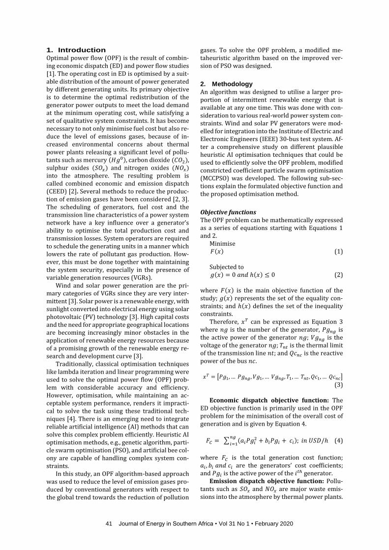
This section presents the outcome of integrating the intermittent renewable generators into the IEEE 30-bus network under the control of the MCCPSO algorithm. Figure 9 represents the propor-tional contribution of the wind, solar PV, and con-ventional generators of the system towards the overall load demand and the total cost of generation (for each hour). It is significant to mention that, in all the presented tables in section 3.5, 𝐶𝑖,𝑊𝑖 𝑎𝑛𝑑 𝑆𝑖 are representing the conventional generators, wind farms and solar farms, respectively.

Figure 9 indicates the varying of the load de-mand conditions where a, b, and c respectively rep-resent the baseload, increased load, and critical load conditions. The load demand conditions were

programmed to consistently alternate over the 24 hours for the sake of analysis, given the intermittent nature of renewable energies. Under each load con-dition, for the first hour, the renewable generators were purposely omitted to investigate the effective-ness of the proposed algorithm on the test system.

Baseload condition The total standard load demand of the IEEE 30-bus network was taken as 283.4 MW, which repre-sented the baseload condition. The simulation pro-duced the optimal dispatching of each generator for every hour through a very detailed cost analysis. Table 8 presents the optimal dispatching of the gen-erators in the standard 30-bus network to meet the baseload demand (1st hour). The outcome was sim-ilar to the CEED results presented in the system analysis before integrating the renewable genera-tors (decimal variation caused by the stochastic na-ture of MCCPSO). Table 9 shows the dispatching of the generators in the network considering renewa-ble power penetration (10th hour).


Figure 9: Integrated system output with respect to the generator schedules.

Table 8: Baseload simulation results at hour 1 (C is the number of conventional generators; W is the number of wind farms; and S is the number of solar farms).

Time step (hour): 1

Load demand: 283.4 MW

Unit Generated power (MW) Generation cost (USD/h) Emission level (kg/h)

C1 123.696 304.769 79.706

C2 49.441 129.299 69.257

C3 29.166 82.333 48.181

C4 31.603 110.999 53.805

C5 27.405 100.991 46.371

C6 28.042 103.785 46.456

W1 0.000 0.000 0.000

W2 0.000 0.000 0.000

W3 0.000 0.000 0.000

S1 0.000 0.000 0.000

The detailed results under the baseload condition without variable generation

Total conventional power 289.353 MW

Total fuel cost 832.1759 USD/h

Total emissions produced 343.7762 kg/h

Overall conventional power cost 1633.312 USD/h

Total wind power 0.000 MW

Total cost of wind power 0.000 USD/h

Total solar PV power 0.000 MW

Total cost of solar PV power 0.000 USD/h

Total power loss 5.953 MW

System power output 289.353 MW

Overall cost of generation 1633.312 USD/h

Elapsed time = 7.884798 seconds.


Table 9: Baseload simulation results at hour 10 (C is the number of conventional generators; W is the number of wind farms and S is the number of solar farms).

Time step (hour): 10

Load demand: 283.4 MW


C1 115.312 280.488 63.681

C2 44.788 113.483 60.953

C3 26.512 70.441 44.217

C4 27.488 95.607 46.750

C5 23.982 86.325 41.283

C6 24.746 89.548 41.759

W1 3.025 5.626 0.000

W2 0.000 0.000 0.000

W3 16.005 29.769 0.000

S1 6.828 15.240 0.000

The detailed results under the baseload condition with variable generation












Elapsed time is 72.392390 seconds.

Figure 10 shows the proportional power gener-

ation at the baseload demand with a reduced pro-duction cost because of the integration of renewa-ble generators. Figure 11 indicates the produced emission volume versus power losses, where the level of emissions produced was significantly re-duced after the system utilised a more significant proportion of available renewable power to meet the baseload demand.

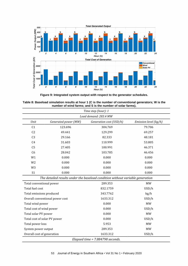
Increased load condition To illustrate the efficiency of the proposed algo-rithm, the load demand was increased to 370 MW. Table 10 represents the second hour of the simula-tion, which presents the outcome of introducing the increased load demand, while omitting any renew-able energy penetration. Table 11 represents the

system with the renewable generators contributing

towards the load demand. The system algorithm ef-

ficiently dispatched all the conventional generators

to meet this load demand without exceeding any of

the generator constraints (evident for the real pow-

ers of generators C4 and C5 in both Tables 10 and

12, respectively) and concerning the availability of

renewable energies. The proportional contribution

of each generator type towards the increased load

demand is shown in Figure 12. There was an in-

crease in the cost of production, level of emissions,

and the power loss as shown in Figures 12 and 13,

respectively. However, with the incorporation of re-

newable energies, these quantities were signifi-

cantly reduced. The renewable generators signifi-

cantly mitigated the level of emissions produced.


Figure 10: Base load operational output.

Figure 11: Generation efficiency at baseload.

Figure 12: Increased load operational output.


Figure 13: Generation efficiency at increased load.

Table 10: Increased load simulation results at hour 2 (C is the number of conventional generators; W is the number of wind farms; and S is the number of solar farms).

Time step (hour): 2

Load demand: 370


The detailed results under the baseload condition with variable generation


Total fuel cost USD/h

Total emissions produced kg/h

Overall conventional power cost USD/h

Total wind power MW

USD/h

Total solar PV power MW

Total cost of solar PV power USD/h

Total power loss MW

System power output MW

Overall cost of generation USD/h

Elapsed time is 14.914027 seconds


Table 11: Increased load simulation results at hour 11 (C is the number of conventional generators; W is the number of wind farms; and S is the number of solar farms).


Load demand: 370 MW


C1 145.311 369.804 129.194

C2 60.836 171.230 93.250

C3 35.369 113.554 58.927

C4 35.000 123.918 60.373

C5 30.000 112.500 50.680

C6 37.123 145.821 62.442

W1 10.983 20.428 0.000

W2 0.000 0.000 0.000

W3 16.005 29.769 0.000

S1 7.851 17.524 0.000

The detailed results under the increased load condition with variable generation


Total fuel cost 1 036.8265 USD/h


Overall conventional power cost 2 096.8439 USD/h







Overall cost of generation 2 164.5656 USD/h


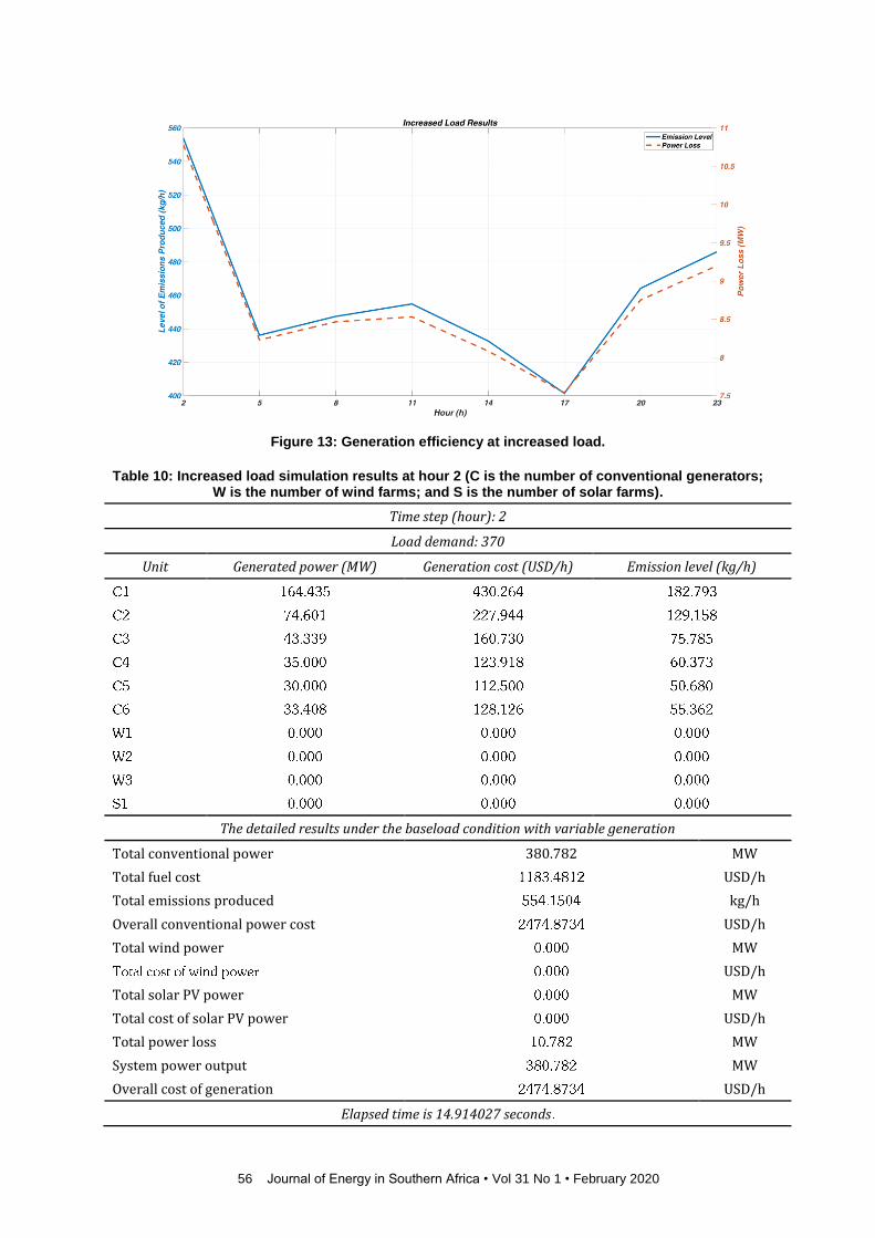
Critical load condition

To test the efficiency of the proposed algorithm at

the extremum points, the load demand was reduced

to 160 MW. This situation is termed as the critical

load condition as it is the initial point where the sys-

tems lower bound constraints might be infringed

upon. Table 12 displays the outcome of the simula-

tion without the output of renewable generators.

Table 13 shows the outcome of the simulation

with renewable energies penetration. The MCCPSO

algorithm efficiently dispatched each generator

without infringing on the inequality constraints of

the conventional generators, while taking into con-

sideration the available renewable power.

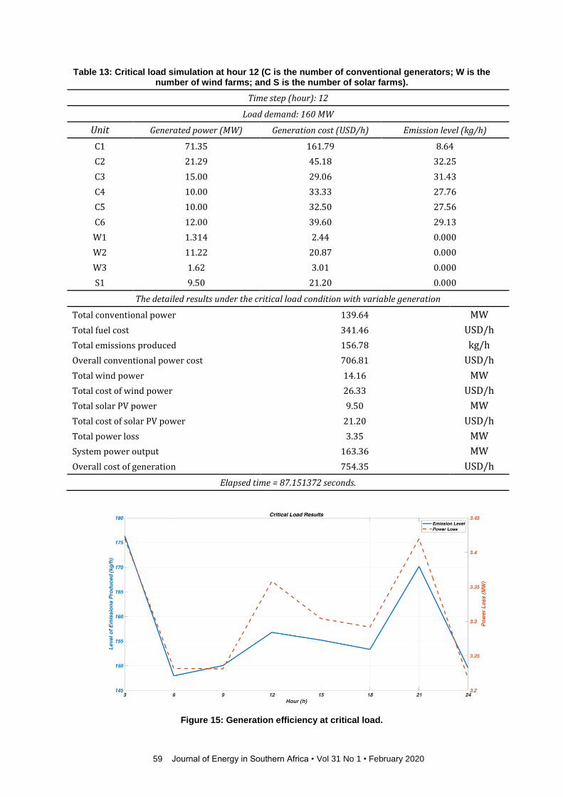
The proportional contribution of each generator

type towards the critical load demand is illustrated

in Figure 14. A decrease was recorded in the cost of

production, the level of emissions produced and the

amount of power loss incurred, as shown in Figures

14 and 15.

4. Conclusions

In this study, an intelligent AC-optimal power flow (AC-OPF) through the adoption of modified con-striction coefficient particle swarm optimisation (MCCPSO) was proposed for solving the dynamic power flow analysis in the presence of variable gen-eration resources (VGRs). The proposed MCCPSO-OPF was designed to interactively incorporate a larger proportion of power supplied by VGRs into the network at any given time, considering the sys-tem security. The MCCPSO-OPF has the unique ca-pability to comprehend and adhere to the physical and systematic operational constraints. The devel-oped MCCPSO-OPF significantly reduced the opera-tion cost and the emission volume by 7.67% and 27%, respectively, for a 24-hour cycle. With respect to the investigated case studies, it can be concluded that the proposed method of the study is able to maximise the social welfare, while minimising the generation costs. It can, therefore, be used by sys-tem operators in the power market industry.


Table 12: Critical load simulation results at hour 3 (C is the number of conventional generators; W is the number of wind farms; and S is the number of solar farms).

Time step (hour): 3

Load demand: 160 MW


C1 83.032 191.917 18.516

C2 27.598 61.626 37.786

C3 17.268 35.903 33.383

C4 12.168 40.775 29.148

C5 11.355 37.287 28.394

C6 12.000 39.600 29.136

W1 0.000 0.000 0.000

W2 0.000 0.000 0.000

W3 0.000 0.000 0.000

S1 0.000 0.000 0.000

The detailed results under the critical load condition without variable generation













Figure 14: Critical load operational output.


Table 13: Critical load simulation at hour 12 (C is the number of conventional generators; W is the number of wind farms; and S is the number of solar farms).


Load demand: 160 MW


C1 71.35 161.79 8.64

C2 21.29 45.18 32.25

C3 15.00 29.06 31.43

C4 10.00 33.33 27.76

C5 10.00 32.50 27.56

C6 12.00 39.60 29.13

W1 1.314 2.44 0.000

W2 11.22 20.87 0.000

W3 1.62 3.01 0.000

S1 9.50 21.20 0.000

The detailed results under the critical load condition with variable generation













Figure 15: Generation efficiency at critical load.


Acknowledgement This work has been supported by the international post-doctoral exchange fellowship programme (Talent-Intro-duction Program) of the People’s Republic of China (Fund No. 207689). Also, the authors would like to sincerely thank the JESA editor (Dr Mok Roberts) for his profes-sional suggestions towards uplifting the technical quality of this research.

Author roles Sumant Lalljith: Formulation of research, computer sim-ulation and execution, data analysis and write-up. Andrew G. Swanson: Manuscript review, data collection, supervision, technical and quality assurance. Arman Goudarzi: Hatched the initial research idea; prob-lem formulation, supervision, computer simulation and write-up.

References [1] Goudarzi, A., Li, Y., & Xiang, J. 2020. A hybrid non-linear time-varying double-weighted particle swarm optimi-

zation for solving non-convex combined environmental economic dispatch problem. Applied Soft Computing, 86, 105894. https://doi.org/10.1016/j.asoc.2019.105894.

[2] Goudarzi, A., Swanson, A. G., Tooryan, F., & Ahmadi, A. 2017. Non-convex optimization of combined environ-mental economic dispatch through the third version of the cultural algorithm. IEEE Texas Power and Energy Conference. https://doi.org/10.1109/tpec.2017.7868281.

[3] Blumsack, S. 2018. Variable energy resources and three economic challenges. The Pennsylvania State Univer-sity. [Online]. Available: https://www.e-education.psu.edu/eme801/node/539. [Accessed 16 July 2018].

[4] Goudarzi, A., Viray, Z. N. C., Siano, P., Swanson, A. G., Coller, J. V., & Kazemi, M. 2017. A probabilistic determina-tion of required reserve levels in an energy and reserve co-optimized electricity market with variable genera-tion. Energy, 130, 258–275. https://doi.org/10.1016/j.energy.2017.04.145.

[5] Velaga, S. & Padma, k. 2013. Combined economic and emission dispatch using multi-objective particle swarm optimization with svc installation. International Journal of Advanced Computer Research, 3(11): 13 – 18. https://doi.org/10.1.1.405.9669.

[6] Monteiro, C., Bessa, R., Miranda, V., Botterud, A., Wang. J., & Conzelmann, G. 2009. Wind power forecasting: state-of-the-art. Decision and Information Services Division, Argonne National Laboratory. 1 – 216. https://doi.org/10.2172/968212.

[7] Borhanazad, H., Mekhilef, S., Gounder Ganapathy, V., Modiri-Delshad, M., & Mirtaheri, A. 2014. Optimization of micro-grid system using mopso. Renewable Energy, 71, 295–306. https://doi.org/10.1016/j.renene.2014.05.006.

[8] Makhloufi, S., Mekhaldi, A., Teguar, M., Koussa, D.S. & Djoudi, A. 2013. Optimal power flow solution including wind power generation into isolated adrar power system using psogsa, Revue des Energies Renouvelables, 16(4): 721 – 732. https://www.semanticscholar.org/.

[9] Abuella, M. A. & Hatziadoniu, C. J. 2015. The economic dispatch for integrated wind power systems using parti-cle swarm optimization. IEEE Conference in Charlotte, 1 – 6. https://arxiv.org/pdf/1509.01693.

[10] Suresh, V. & Suresh, S. 2015. Economic dispatch and cost analysis on a power system network interconnected with solar farm. International Journal of Renewable Energy Research, 5(4):1099 – 1105. https://www.ijrer.org/.

[11] ElDesouky, A. A. 2013. Security and stochastic economic dispatch of power system including wind and solar resources with environmental consideration. International Journal of Renewable Energy Research, 3(4): 951 – 958. https://www.ijrer.org/.

[12] Saxena, N., & Ganguli, S. 2015. Solar and wind power estimation and economic load dispatch using firefly algo-rithm. Procedia Computer Science, 70, 688–700. https://doi.org/10.1016/j.procs.2015.10.106.

[13] Saadat, H. 1999. Power System Analysis. New York, WCB/McGraw-Hill. https://www.mheducation.com/.

[14] Sereeter, B., Vuik, C., & Witteveen, C. 2019. On a comparison of Newton–Raphson solvers for power flow prob-lems. Journal of Computational and Applied Mathematics, 360, 157–169. https://doi.org/10.1016/j.cam.2019.04.007.

[15] Aslam, M. U., Cheema, M. U., Samran, M., & Cheema, M. B. 2014. Optimal power flow based upon genetic algo-rithm deploying optimum mutation and elitism. The 1st International Conference on Information Technology, Computer, and Electrical Engineering. https://doi.org/10.1109/icitacee.2014.7065767.

[16] Goudarzi, A., Ahmadi, A., Swanson, A. G., & Van Coller, J. 2016. Non-convex optimisation of combined environ-mental economic dispatch through cultural algorithm with the consideration of the physical constraints of gen-erating units and price penalty factors. SAIEE Africa Research Journal, 107(3), 146–166. https://doi.org/10.23919/saiee.2016.8532239.

[17] Pranava, G., & Prasad, P. V. 2013. Constriction coefficient particle swarm optimization for economic load dis-patch with valve point loading effects. International Conference on Power, Energy and Control. https://doi.org/10.1109/icpec.2013.6527680.

[18] Fahad, S., Mahdi, A. J., Tang, W. H., Huang, K., & Liu, Y. 2018. Particle swarm optimization based dc-link voltage control for two stage grid connected pv inverter. International Conference on Power System Technology. https://doi.org/10.1109/powercon.2018.8602128.

https://doi.org/10.1016/j.asoc.2019.105894

https://doi.org/10.1016/j.asoc.2019.105894

https://doi.org/10.1109/tpec.2017.7868281

https://doi.org/10.1109/tpec.2017.7868281

https://www.e-education.psu.edu/eme801/node/539

https://www.e-education.psu.edu/eme801/node/539

https://doi.org/10.1016/j.energy.2017.04.145

https://doi.org/10.1016/j.energy.2017.04.145

https://doi.org/10.1.1.405.9669

https://doi.org/10.1.1.405.9669

https://doi.org/10.2172/968212

https://doi.org/10.2172/968212

https://doi.org/10.1016/j.renene.2014.05.006

https://doi.org/10.1016/j.renene.2014.05.006

https://www.semanticscholar.org/


https://arxiv.org/pdf/1509.01693

https://arxiv.org/pdf/1509.01693

https://www.ijrer.org/




https://doi.org/10.1016/j.procs.2015.10.106

https://doi.org/10.1016/j.procs.2015.10.106

https://www.mheducation.com/

https://www.mheducation.com/

https://doi.org/10.1016/j.cam.2019.04.007

https://doi.org/10.1016/j.cam.2019.04.007

https://doi.org/10.1109/icitacee.2014.7065767

https://doi.org/10.1109/icitacee.2014.7065767

https://doi.org/10.23919/saiee.2016.8532239

https://doi.org/10.23919/saiee.2016.8532239

https://doi.org/10.1109/icpec.2013.6527680

https://doi.org/10.1109/icpec.2013.6527680

https://doi.org/10.1109/powercon.2018.8602128

https://doi.org/10.1109/powercon.2018.8602128


[19] Gharib, A., Benhra, J. & Chaouqi, M. 2018. A performance comparison of genetic algorithm and particle swarm optimization applied to tsp. International Journal of Recent Trends in Engineering and Research, 4(4), 529–536. https://doi.org/10.23883/ijrter.2018.4270.s3bvz.

[20] Caboz, J. 2018. These are the 5 biggest green energy projects in SA – all wind farms. Business Inside. [Online]. Available: https://www.businessinsider.co.za/5-massive-new-renewable-energy-projects-that-transformed-south-africas-landscape-2018-4. [Accessed 7 September 2018].

[21] Suzlon Energy Limited. Suzlon powering a greener tomorrow. classic fleet, [Online]. Available: https://www.suzlon.com/in-en/energy-solutions/classic-fleet-wind-turbines. [Accessed 17 September 2018].

[22] The Nordex Group. AW3000 – Nordex. [Online]. Available: http://www.nordex-online.com/fileadmin/ME-DIA/AW/AW3000_oct17_EU-EN.pdf&ved=2ahUKEwiVhJCIyffdAhUDXsAKHQfzCvMQFjAAegQIA-hAB&usg=AOvVaw0oLQyNN65v-IWmyamss9Kz. [Accessed 8 September 2018].

[23] The Nordex Group. Nordex: N117/3000. [Online]. Available: www.nordex-online.com/en/produkte-ser-vice/wind-turbines/n117-30-mw.html. [Accessed 8 September 2018].

[24] South African Wind Energy Association. Wind energy. [Online]. Available: www.sawea.org.za. [Accessed 10 September 2018].

[25] Southern African Universities Radiometric Network. Solar radiometric data for the public sauran, Durban. http://www.sauran.net/ShowStation.aspx?station=2.

[26] Aryal, A., & Bhattarai, N. 2018. Modelling and simulation of 115.2 kwp grid-connected solar pv system using pvsyst. Kathford Journal of Engineering and Management, 1(1), 31–34. https://doi.org/10.3126/kjem.v1i1.22020.

[27] Oubbati, Y., Mohammed, A. & Arif, S. 2016. Improved pso applied to the optimal power flow with transient sta-bility constraints. Journal of Electrical Systems, 12(4): 672 – 686. https://creativecommons.org/licenses/by-nc/4.0/.

[28] Reddy, S. S., & Momoh, J. A. 2016. Minimum emission dispatch in an integrated thermal and wind energy con-servation system using self-adaptive differential evolution. IEEE PES Power Africa. https://doi.org/10.1109/powerafrica.2016.7556615.

[29] Panda, S.R. 2013. Distributed slack bus model for qualitative economic load dispatch. National Institute of Technology, Rourkela, 1 – 45. https://www.semanticscholar.org/.

[30] Augusteen, W. A., Geetha, S., & Rengaraj, R. 2016. Economic dispatch incorporation solar energy using particle swarm optimization. 3rd International Conference on Electrical Energy Systems. https://doi.org/10.1109/icees.2016.7510618.

[31] Garnham, B. L. 2016. Mercury emissions from South Africa’s coal-fired power stations. Clean Air Journal, 26(2), 14–20. https://doi.org/10.17159/2410-972x/2016/v26n2a8.

https://doi.org/10.23883/ijrter.2018.4270.s3bvz

https://www.businessinsider.co.za/5-massive-new-renewable-energy-projects-that-transformed-south-africas-landscape-2018-4




https://www.suzlon.com/in-en/energy-solutions/classic-fleet-wind-turbines

https://www.suzlon.com/in-en/energy-solutions/classic-fleet-wind-turbines

http://www.nordex-online.com/fileadmin/MEDIA/AW/AW3000_oct17_EU-EN.pdf&ved=2ahUKEwiVhJCIyffdAhUDXsAKHQfzCvMQFjAAegQIAhAB&usg=AOvVaw0oLQyNN65v-IWmyamss9Kz






http://www.nordex-online.com/en/produkte-service/wind-turbines/n117-30-mw.html




http://www.sawea.org.za/

http://www.sawea.org.za/

http://www.sauran.net/ShowStation.aspx?station=2

http://www.sauran.net/ShowStation.aspx?station=2

https://doi.org/10.3126/kjem.v1i1.22020

https://doi.org/10.3126/kjem.v1i1.22020

https://creativecommons.org/licenses/by-nc/4.0/




https://doi.org/10.1109/powerafrica.2016.7556615

https://doi.org/10.1109/powerafrica.2016.7556615



https://doi.org/10.1109/icees.2016.7510618

https://doi.org/10.1109/icees.2016.7510618

https://doi.org/10.17159/2410-972x/2016/v26n2a8

https://doi.org/10.17159/2410-972x/2016/v26n2a8

an intelligent alternating current-optimal power flow for

Documents