an integrated supplier selection model with product life
TRANSCRIPT

The Pennsylvania State University
The Graduate School
The Harold and Inge Marcus
Department of Industrial and Manufacturing Engineering
An Integrated Supplier Selection Model with Product
Life Cycle Considerations
A Dissertation in
Industrial Engineering
by
Richard John Titus, Jr.
Submitted in Partial Fulfillment
of the Requirements
for the Degree of
Doctor of Philosophy
May 2019

ii
The dissertation of Richard John Titus, Jr. was reviewed and approved* by the following:
Ravi Ravindran
Professor Emeritus of Industrial Engineering
Dissertation Adviser
Chair of Committee
Felisa Preciado Higgins
Clinical Associate Professor of Supply Chain Management
Smeal College of Business
El-Amine Lehtihet
Professor of Industrial Engineering
Vittaldas Prabhu
Professor of Industrial Engineering
Janis Terpenny
Head of the Department of Industrial and Manufacturing Engineering
*Signatures are on file in the Graduate School

iii
Abstract
Cost of purchased materials account for up to 70% of the overall product cost and the
consequences of supplier delivery, quality performance problems and price fluctuations
can have profound negative effects for an organization. Product life cycles are increasing
in length for defense applications and shortening in consumer products, such as toys,
electronics, etc. These factors make the purchasing function a critical factor impacting the
long term health of companies.
In this dissertation, we begin with the investigation of the relationship between supplier
quality and delivery performance and supplier attributes as part of an empirical study using
an ordinal logistic regression. The results of this study are utilized to develop an integrated
supplier selection model with product life cycle considerations. Supplier selection is a
multiple criteria optimization problem with conflicting criteria, such as quality, delivery,
service, product safety and others. Several multiple criteria sourcing models exist in the
literature. Very rarely they have considered the fact that the relative importance of the
supplier attributes depends on the product life cycle phase. For example, during the
Introduction phase, companies may work with a single supplier emphasizing product
safety, quality and delivery. Revenue targets are more important than gross profit margins.
However, during the Growth phase, multiple suppliers may be used to meet surging
demand and to introduce price competition among the suppliers. In the Mature phase,
controlling procurement cost becomes important in order to boost the product gross profit
margin. In addition, many suppliers can deliver materials needed for multiple products
under various stages of the product life cycle phase. Companies may also limit the business
volume to new and existing suppliers. All these factors are integrated into a general model.
In this thesis, a multiple criteria, multiple products, supplier selection model that explicitly
considers the product life cycle phases of the products is developed. The Goal
Programming (GP) approach is used to solve the multiple criteria problem. The general
model objectives include price, lead-time, quality, delivery, product performance and
safety. Products from the introduction, growth, maturity and decline phases of the product
life cycle are included in the general model. An illustrative example is developed and a

iv
number of goal programming approaches, including preemptive, non-preemptive,
Tchebycheff’s min-max and fuzzy, are utilized to provide the optimal solutions. The Value
Path method is used to provide visual tradeoffs of the conflicting objectives across the
product life cycle phases.
This general model is applied to a real-world problem. The case study is focused on a U.S.
based consumer products company which utilizes a diverse global supply chain to design,
manufacture and deliver products throughout the world. Three key executive decision
makers are employed to identify and rank the key sourcing criteria attributes for products
representing the introduction, growth, mature and decline phases of the product life cycle.
Ranking methods included rating method, Borda count utilizing pairwise comparisons and
the Analytic Hierarchy Process. The decision makers (DMs) shared their feedback on the
cognitive burden for each of the ranking methods. Ranking results indicate that the DM’s
priorities change based on the product life cycle phase. A number of constraints based on
the company’s procurement practices were include in creating the supplier selection
models. The GP model results, for the preemptive, non-preemptive and Tchebycheff’s
min-max models, were presented to the decision makers utilizing the Value Path method.
The decision makers quickly understood the significance of Value Path graphs and focused
on choosing the best overall sourcing solutions based on their rankings of the supplier
attributes.
In order to test the effectiveness of the model, the actual orders used by the company were
compared to the GP model results. A number of factors impacted the actual order
allocations, such as unanticipated demand, supplier capacity constraints and supply chain
designs. The GP model results exceeded the actual order allocation’s criteria performance
for many of the products throughout the product life cycle phases. A comparison of the
actual procurement cost with those of the GP models showed substantial cost savings to
the company, while maintaining quality, delivery and safety performance. These results
were presented to the company’s Chief Operating Officer using the Value Path approach.
He provided extensive feedback and had questions on how the model results could be
blended to examine alternate solutions. He was able to identify opportunities for the

v
company to improve supplier performance in an effort to minimize supplier risk. This
reveals the strength of this integrated decision-making model, which allows “what if”
scenarios to be tried, including changing goal priority weights, priorities and relaxing
business constraints and thus provide the DM with alternative sourcing strategies to
consider.

vi
Table of Contents List of Figures .................................................................................................................... xi
List of Tables ................................................................................................................... xiii
Acknowledgments............................................................................................................ xix
1. Introduction .................................................................................................................... 1
1.1 Problem Statement ............................................................................................... 4
1.2 Motivation for the Thesis ..................................................................................... 5
1.3 Overview of the Thesis ........................................................................................ 7
2. Literature Review ......................................................................................................... 10
2.1 The Importance of Supplier Selection and Management Processes .................. 10
2.2 Supplier Criteria Development and Selection Methodologies ........................... 11
2.2.1 MCDM Models ........................................................................................... 12
2.2.2 Supplier Criteria Determination and Supplier Selection ............................ 23
2.3 Risk and Supplier Selection ............................................................................... 32
2.4 The Product Life Cycle and Supplier Selection ................................................. 35
3. Empirical Study of Supplier Attributes to Supplier Delivery and Quality Performance .
................................................................................................................................... 39
3.1 Hypothesis Development and Research Methodology ...................................... 40
3.2 Hypothesized Impact of Critical Attributes on Quality and Delivery
Performance ....................................................................................................... 42
3.3 Delivery and Quality Dependent Variables Defined.......................................... 44
3.4 Quality Ratings and Technical Capability as it Relates to Delivery and Quality
Performance ....................................................................................................... 47
3.5 Financial Condition and Supplier Payment Performance as it Relates to Delivery
and Quality Performance ................................................................................... 49
3.6 Product Complexity and Differentiation as it Relates to Delivery and Quality
Performance ....................................................................................................... 51
3.7 Number of Employees as it Relates to Delivery and Quality Performance ....... 53
3.8 Distance as it Relates to Delivery Performance ................................................. 55
3.9 Financial Leverage or Purchasing Power as it Relates to Delivery and Quality
Performance ....................................................................................................... 56
3.10 Case Study Model Selection and Results.............................................................. 58
3.10.1 Model Selection....................................................................................... 58
3.10.2 Variable Definitions for Number of Employees and Financial or
Purchasing Leverage ................................................................................. 60
3.10.3 Summary Statistics .................................................................................. 62

vii
3.10.4 Model Definitions and Results ................................................................ 63
3.10.5 Empirical Study Conclusions and Implications for the Supplier Selection
Process and MCDM Model Formulations ................................................ 65
4. General Model for Supplier Selection incorporating results of Empirical Study and
Product Life Cycle ........................................................................................................ 70
4.1 Notations used in the model ............................................................................... 71
4.2 Mathematical Formulation of the Order Allocation Problem ............................ 73
4.2.1 Objective Functions .................................................................................... 73
4.2.2 Constraints .................................................................................................. 76
4.3 Goal Programming (GP) Models ....................................................................... 78
4.3.1 Ideal Solutions ............................................................................................ 78
4.3.2 General Goal Programming Model ............................................................. 79
4.3.3 Preemptive Goal Programming Model ....................................................... 82
4.3.4 Non-preemptive Goal Programming Model ............................................... 83
4.3.5 Tchebycheff’s Min-Max Goal Programming Model .................................. 83
4.3.6 Fuzzy Goal Programming Model................................................................ 84
4.4 Illustrative Example ........................................................................................... 84
4.4.1 Ideal Solutions ............................................................................................ 84
4.4.2 Preemptive Goal Programming Results ...................................................... 87
4.4.3 Non-Preemptive Goal Programming Results.............................................. 94
4.4.3 Tchebycheff’s (Min-Max) Goal Programming ......................................... 104
4.4.3 Fuzzy Goal Programming ......................................................................... 108
4.4.4 Overall Model Results .............................................................................. 111
4.4.7 Chapter Conclusion ................................................................................... 117
5. Case Study: Global Supplier Selection Problem across Product Life Cycle – Supplier
Ranking Results .......................................................................................................... 118
5.1 Background of the Company and the Decision Makers ................................... 118
5.2 Description of Products and Suppliers ............................................................. 120
5.3 Key Supplier Selection Criteria........................................................................ 122
5.4 Ranking the Product Life Cycle Phases ........................................................... 125
5.5 Ranking the Supplier Selection Criteria by PLC Phase ................................... 130
5.5.1 Ranking the Supplier Selection Criteria by DM1 .................................... 130
5.5.2 Ranking the Supplier Selection Criteria by DM2 .................................... 132
5.5.3 Ranking the Supplier Selection Criteria by DM3 ..................................... 133
5.6 Final Ranking and Weights for the MCDM Supplier Selection Models ......... 135

viii
5.6.1 Ranking and Weights of PLC Phases ....................................................... 135
5.6.2 Final Criteria Weights by PLC Phase ....................................................... 136
5.6.3 Overall Weights for the Goal Programming Models ................................ 136
5.7 Minimum and Maximum Number of Suppliers by PLC Phase ....................... 138
6. Case Study: Global Supplier Selection Problem across Product Life Cycle – Supplier
Selection and Order Allocation .................................................................................. 140
6.1 Preemptive GP Model for the Case Study ....................................................... 140
6.1.1 Preemptive GP Priorities.......................................................................... 141
6.1.2 Preemptive GP Solution ........................................................................... 143
6.1.3 Introduction Phase Results (Product 1).................................................... 143
6.1.4 Introduction Phase Results (Product 2).................................................... 144
6.1.5 Growth Phase Results (Product 3) ........................................................... 145
6.1.6 Mature Phase Results (Product 4) ............................................................ 147
6.1.7 Mature Phase Results (Product 5) ............................................................ 148
6.1.8 Decline Phase Results (Product 6) ........................................................... 149
6.1.9 Decline Phase Results (Product 7) ........................................................... 150
6.1.10 Optimal Order Allocations to Suppliers (All Products) ........................ 151
6.2 Non-Preemptive GP Model for the Case Study ............................................... 153
6.2.1 Non-Preemptive GP Model Weights and Solution .................................. 153
6.2.2 Introduction Phase Results (Product 1).................................................... 154
6.2.3 Introduction Phase Results (Product 2).................................................... 155
6.2.4 Growth Phase Results (Product 3) ........................................................... 156
6.2.5 Mature Phase Results (Product 4) ............................................................ 157
6.2.6 Mature Phase Results (Product 5) ............................................................ 158
6.2.7 Decline Phase Results (Product 6) ........................................................... 159
6.2.8 Decline Phase Results (Product 7) ........................................................... 160
6.2.9 Optimal Order Allocations to Suppliers (All Products) ........................... 161
6.3 Tchebycheff’s Min-Max GP Model for the Case Study ....................................... 162
6.3.1 Tchebycheff’s Min-Max Goals/Targets and Solution ............................. 162
6.3.2 Introduction Phase Results (Product 1).................................................... 163
6.3.3 Introduction Phase Results (Product 2).................................................... 164
6.3.4 Growth Phase Results (Product 3) ........................................................... 165
6.3.5 Mature Phase Results (Product 4) ............................................................ 166
6.3.6 Mature Phase Results (Product 5) ............................................................ 167
6.3.7 Decline Phase Results (Product 6) ........................................................... 168

ix
6.3.8 Decline Phase Results (Product 7) ........................................................... 170
6.3.9 Optimal Order Allocations to Suppliers (All Products) ........................... 171
6.4 Fuzzy Min-Max GP Model for the Case Study .................................................... 172
6.4.1 Fuzzy Min-Max Ideals and Solution........................................................ 172
6.4.2 Introduction Phase Results (Product 1).................................................... 173
6.4.3 Introduction Phase Results (Product 2).................................................... 174
6.4.4 Growth Phase Results (Product 3) ........................................................... 175
6.4.5 Mature Phase Results (Product 4) ............................................................ 176
6.4.6 Mature Phase Results (Product 5) ............................................................ 177
6.4.7 Decline Phase Results (Product 6) ........................................................... 178
6.4.8 Decline Phase Results (Product 7) ........................................................... 179
6.4.9 Optimal Order Allocations to Suppliers (All Products) ........................... 180
6.5 Value Path Results ................................................................................................ 182
6.5.1 Introduction Phase (Product 1) ................................................................ 182
6.5.2 Introduction Phase (Product 2) ................................................................ 185
6.5.3 Growth Phase (Product 3) ........................................................................ 188
6.5.4 Mature Phase (Product 4)......................................................................... 190
6.5.5 Mature Phase (Product 5)......................................................................... 193
6.5.6 Decline Phase (Product 6) ........................................................................ 195
6.5.7 Decline Phase (Product 7) ........................................................................ 197
6.6 Managerial Implications ................................................................................... 199
6.6.1 Actual Order Allocations ......................................................................... 200
6.6.2 Introduction Phase (Product 1) ................................................................ 201
6.6.3 Introduction Phase (Product 2) ................................................................ 205
6.6.4 Growth Phase (Product 3) ........................................................................ 209
6.6.5 Mature Phase (Product 4)......................................................................... 211
6.6.6 Mature Phase (Product 5)......................................................................... 215
6.6.7 Decline Phase (Product 6) ........................................................................ 218
6.6.8 Decline Phase (Product 7) ........................................................................ 221
6.6.9 Impact on Procurement Cost .................................................................... 223
6.7 Chapter Summary ............................................................................................. 228
7. Conclusion and Future Research ................................................................................ 232
7.1 Summary of Model Contributions to Supplier Selection ................................. 232
7.2 Summary of Practical Significance .................................................................. 234

x
7.3 Future Research Opportunities ......................................................................... 237
References ....................................................................................................................... 239

xi
List of Figures
Figure 1.1 Supply Segmentation Model ..............................................................................3
Figure 2.1 Selecting and Managing Suppliers ...................................................................10
Figure 3.1 Supplier Attributes and Performance Relationship ..........................................43
Figure 3.2 Hypothesized Relationships with Delivery and Quality Performance .............44
Figure 4.1 Illustrative Weights for the Non-preemptive GP Models.................................97
Figure 4.2 Non-Preemptive GP Model Goal Weights vs. Target Achievements ............103
Figure 4.3 Value Path Model Results Comparison ..........................................................114
Figure 5.1 Product Life Cycle Responses from DM1......................................................126
Figure 6.1 Fuzzy GP Results ...........................................................................................181
Figure 6.2 Value Path Model Results Comparison for Introduction Phase Product 1 ....185
Figure 6.3 Value Path Model Results Comparison for Introduction Phase Product 2 ....187
Figure 6.4 Value Path Model Results Comparison for Growth Phase Product 3 ............190
Figure 6.5 Value Path Model Results Comparison for Mature Phase Product 4 .............192
Figure 6.6 Value Path Model Results Comparison for Mature Phase Product 5 .............195
Figure 6.7 Value Path Model Results Comparison for Decline Phase Product 6 ............197
Figure 6.8 Value Path Model Results Comparison for Decline Phase Product 7 ............199
Figure 6.9 DM Review of the Value Path Calculations for Introduction Phase Product 1
..............................................................................................................................204
Figure 6.10 Value Path Graph: Comparison of Actual Orders and Model Results for
Introduction Phase Product 1 ...............................................................................204
Figure 6.11 DM Review Actual Orders and GP Model Allocations and Value Path Graph
for Introduction Phase Product 1 ..........................................................................205
Figure 6.12 Value Path Graph: Comparison of Actual Orders and Model Results for
Introduction Phase Product 2 ...............................................................................207
Figure 6.13 DM Review Actual Orders and GP Model Allocations and Value Path Graph
for Introduction Phase Product 2 ..........................................................................208
Figure 6.14 Value Path Graph: Comparison of Actual Orders and Model Results for
Growth Phase Product 3 .......................................................................................210
Figure 6.15 DM Review Actual Orders and GP Model Allocations and Value Path Graph
for Mature Phase Product 4 ..................................................................................213
Figure 6.16 Value Path Graph: Comparison of Actual Orders and Model Results for Mature
Phase Product 4 ....................................................................................................214
Figure 6.17 Value Path Actual Orders and Model Results Comparison for Mature Phase
Product 5 ...............................................................................................................217

xii
Figure 6.18 Value Path Actual Orders and Model Results Comparison for Decline Phase
Product 6 ...............................................................................................................220
Figure 6.19 Value Path Actual Orders and Model Results Comparison for Decline Phase
Product 7 ...............................................................................................................222
Figure 6.20 Procurement Cost Comparison of Actual Orders and GP Models for
Introduction Phase Products 1 and 2 ....................................................................223
Figure 6.21 Procurement Cost Comparison of Actual Orders and GP Models for Growth
Phase Product 3 and Mature Phase Products 4 and 5 ...........................................224
Figure 6.22 Procurement Cost Comparison of Actual Orders and GP Models for Decline
Phase Products 6 and 7 .........................................................................................227
Figure 6.23 DM Review of the Price Achievements for Actual Order and GP Models..228

xiii
List of Tables
Table 2.1 Supplier Selection Criteria Comparison ............................................................11
Table 2.2 Supplier Criteria and Selection Literature Summary .........................................38
Table 3.1 Delivery Performance Rating ............................................................................45
Table 3.2 Quality Performance Rating ..............................................................................46
Table 3.3 Financial Condition Rating ................................................................................49
Table 3.4 Supplier Payment Performance Rating ..............................................................50
Table 3.5 Distance (Mileage) Rating Scale .......................................................................55
Table 3.6 Employee Rating Scale ......................................................................................60
Table 3.7 Financial Leverage or Purchasing Leverage Rating Scale ................................61
Table 3.8 Summary Statistics ............................................................................................62
Table 3.9 Summarized Results for the Supplier Quality and Delivery Models.................65
Table 3.10 Ordinal Logistic Regression Results for Supplier Quality Performance .........67
Table 3.11 Ordinal Logistic Regression Results for Supplier Delivery Performance .......68
Table 4.1 Supplier Data for Illustrative Example ..............................................................85
Table 4.2 Ideal Solutions for the Illustrative Example ......................................................86
Table 4.3 Preemptive Goal Priority Order .........................................................................88
Table 4.4 Preemptive GP Achievements with respect to Target Values ...........................92
Table 4.5 Preemptive GP Procurement Plan......................................................................93
Table 4.6 Allocation of Weights by Objective for Non-Preemptive GP Model ................96
Table 4.7 Non-preemptive GP Achievements with respect to Target Values .................100
Table 4.8 Non-preemptive GP Procurement Plan............................................................100
Table 4.9 Tchebycheff’s Min-Max GP Achievements with respect to Target Values ....105
Table 4.10 Tchebycheff’s Min-Max GP Procurement Plan ............................................105
Table 4.11 Fuzzy GP Achievements with respect to Ideal Values ..................................109
Table 4.12 Fuzzy GP Procurement Plan ..........................................................................109
Table 4.13 Model Results and Target Values ..................................................................112
Table 4.14 Value Path Results .........................................................................................113
Table 5.1 Products and Suppliers for Case Study ............................................................120
Table 5.2 Yearly Unit Product Demand ..........................................................................121
Table 5.3 Supplier Performance Ratings and Maximum Business Levels ......................124
Table 5.4 Ranking of PLC Phases by Different Methods for DM1.................................127
Table 5.5 Ranking of PLC Phases by Different Methods for DM2.................................128
Table 5.6 Ranking of PLC Phases by Different Methods for DM3.................................129

xiv
Table 5.7 DM1’s Ranking of Criteria for Introduction and Growth Phases by Different
Methods .................................................................................................................130
Table 5.8 DM1’s Ranking of Criteria for Mature and Decline Phases by Different Methods
...............................................................................................................................131
Table 5.9 DM2’s Ranking of Criteria for Introduction and Growth Phases by Different
Methods .................................................................................................................132
Table 5.10 DM2’s Ranking of Criteria for Mature and Decline Phases by Different
Methods .................................................................................................................133
Table 5.11 DM3’s Ranking of Criteria for Introduction and Growth Phases by Different
Methods .................................................................................................................134
Table 5.12 DM3’s Ranking of Criteria for Mature and Decline Phases by Different
Methods .................................................................................................................134
Table 5.13 Average AHP weights by PLC Phase ............................................................136
Table 5.14 Average AHP Weights by PLC Phase and Supplier Selection Criteria ........137
Table 5.15 Overall AHP Weights for Goal Programming ...............................................137
Table 5.16 Number of Suppliers by PLC Phase ..............................................................138
Table 6.1 Preemptive GP Model Characteristics for the Case Study ..............................140
Table 6.2 Preemptive GP Supplier Selection Priorities ...................................................142
Table 6.3 Preemptive GP Procurement Plan for Introduction Phase Product 1 ..............143
Table 6.4 Preemptive GP Achievements for Introduction Phase Product 1 with respect to
Target Values ........................................................................................................144
Table 6.5 Preemptive GP Procurement Plan for Introduction Phase Product 2 ..............144
Table 6.6 Preemptive GP Achievements for Introduction Phase Product 2 with respect to
Target Values .........................................................................................................145
Table 6.7 Preemptive GP Procurement Plan for Growth Phase Product 3 ......................146
Table 6.8 Preemptive GP Achievements for Growth Phase Product 3 with respect to Target
Values ....................................................................................................................146
Table 6.9 Preemptive GP Procurement Plan for Mature Phase Product 4 .......................147
Table 6.10 Preemptive GP Achievements for Mature Phase Product 4 with respect to
Target Values .........................................................................................................148
Table 6.11 Preemptive GP Procurement Plan for Mature Phase Product 5 .....................149
Table 6.12 Preemptive GP Achievements for Mature Phase Product 5 with respect to
Target Values .........................................................................................................149
Table 6.13 Preemptive GP Procurement Plan for Decline Phase Product 6 ....................149
Table 6.14 Preemptive GP Achievements for Decline Phase Product 6 with respect to
Target Values .........................................................................................................150
Table 6.15 Preemptive GP Procurement Plan for Decline Phase Product 7 ....................151

xv
Table 6.16 Preemptive GP Achievements for Decline Phase Product 7 with respect to
Target Values .........................................................................................................151
Table 6.17 Preemptive GP Procurement Plan (All Products) ..........................................152
Table 6.18 Non-preemptive GP Model Characteristics for the Case Study ....................153
Table 6.19 Non-preemptive GP Weights .........................................................................154
Table 6.20 Non-preemptive GP Procurement Plan for Introduction Phase Product 1 ....154
Table 6.21 Non-preemptive GP Achievements for Introduction Phase Product 1 with
respect to Target Values ........................................................................................155
Table 6.22 Non-preemptive GP Procurement Plan for Introduction Phase Product 2 ....155
Table 6.23 Non-preemptive GP Achievements for Introduction Phase Product 2 with
respect to Target Values ........................................................................................156
Table 6.24 Non-preemptive GP Procurement Plan for Growth Phase Product 3 ............156
Table 6.25 Non-preemptive GP Achievements for Growth Phase Product 3 with respect to
Target Values .........................................................................................................157
Table 6.26 Non-preemptive GP Procurement Plan for Mature Phase Product 4.............157
Table 6.27 Non-preemptive GP Achievements for Mature Phase Product 4 with respect to
Target Values .........................................................................................................158
Table 6.28 Non-preemptive GP Procurement Plan for Mature Phase Product 5.............159
Table 6.29 Non-preemptive GP Achievements for Mature Phase Product 5 with respect to
Target Values .........................................................................................................159
Table 6.30 Non-preemptive GP Procurement Plan for Mature Phase Product 6.............160
Table 6.31 Non-preemptive GP Achievements for Decline Phase Product 6 with respect to
Target Values .........................................................................................................160
Table 6.32 Non-preemptive GP Procurement Plan for Mature Phase Product 7.............160
Table 6.33 Non-preemptive GP Achievements for Decline Phase Product 7 with respect to
Target Values .........................................................................................................161
Table 6.34 Non-preemptive GP Procurement Plan (All Products) ..................................162
Table 6.35 Tchebycheff’s Min-Max GP Model Characteristics for the Case Study .......162
Table 6.36 Tchebycheff’s Min-Max GP Procurement Plan for Introduction Phase Product
1 .............................................................................................................................163
Table 6.37 Tchebycheff’s GP Achievements for Introduction Phase Product 1 with respect
to Target Values .....................................................................................................163
Table 6.38 Tchebycheff’s Min-Max GP Procurement Plan for Introduction Phase Product
2 ............................................................................................................................164
Table 6.39 Tchebycheff's GP Achievements for Introduction Phase Product 2 with respect
to Target Values .....................................................................................................164
Table 6.40 Tchebycheff’s Min-Max GP Procurement Plan for Growth Phase Product 3
...............................................................................................................................165

xvi
Table 6.41 Tchebycheff’s GP Achievements for Growth Phase Product 3 with respect to
Target Values .........................................................................................................165
Table 6.42 Tchebycheff’s Min-Max GP Procurement Plan for Mature Phase Product 4
...............................................................................................................................166
Table 6.43 Tchebycheff’s GP Achievements for Mature Phase Product 4 with respect to
Target Values .........................................................................................................167
Table 6.44 Tchebycheff’s Min-Max GP Procurement Plan for Mature Phase Product 5
...............................................................................................................................167
Table 6.45 Tchebycheff’s GP Achievements for Mature Phase Product 5 with respect to
Target Values .........................................................................................................168
Table 6.46 Tchebycheff’s Min-Max GP Procurement Plan for Decline Phase Product 6
...............................................................................................................................168
Table 6.47 Tchebycheff’s GP Achievements for Decline Phase Product 6 with respect to
Target Values .........................................................................................................169
Table 6.48 Tchebycheff’s Min-Max GP Procurement Plan for Decline Phase Product 7
...............................................................................................................................170
Table 6.49 Tchebycheff’s GP Achievements for Decline Phase Product 7 with respect to
Target Values .........................................................................................................170
Table 6.50 Tchebycheff’s Min-Max GP Procurement Plan (All Products) .....................171
Table 6.51 Fuzzy Min-Max GP Model Characteristics for the Case Study ....................172
Table 6.52 Fuzzy Min-Max GP Procurement Plan for Introduction Phase Product 1 ....173
Table 6.53 Fuzzy GP Achievements for Introduction Phase Product 1 with respect to Ideal
Values ....................................................................................................................173
Table 6.54 Fuzzy GP Procurement Plan for Introduction Phase Product 2 .....................174
Table 6.55 Fuzzy GP Achievements for Introduction Phase Product 2 with respect to Ideal
Values ....................................................................................................................174
Table 6.56 Fuzzy GP Procurement Plan for Growth Phase Product 3 ............................175
Table 6.57 Fuzzy GP Achievements for Growth Phase Product 3 with respect to Ideal
Values ....................................................................................................................175
Table 6.58 Fuzzy GP Procurement Plan for Mature Phase Product 4 .............................176
Table 6.59 Fuzzy GP Achievements for Mature Phase Product 4 with respect to Ideal
Values ....................................................................................................................176
Table 6.60 Fuzzy GP Procurement Plan for Mature Phase Product 5 .............................177
Table 6.61 Fuzzy GP Achievements for Mature Phase Product 5 with respect to Ideal
Values ....................................................................................................................178
Table 6.62 Fuzzy GP Procurement Plan for Decline Phase Product 6 ............................178
Table 6.63 Fuzzy GP Achievements for Mature Phase Product 6 with respect to Ideal
Values ....................................................................................................................179

xvii
Table 6.64 Fuzzy GP Procurement Plan for Decline Phase Product 7 ............................179
Table 6.65 Fuzzy GP Achievements for Decline Phase Product 7 with respect to Ideal
Values ....................................................................................................................180
Table 6.66 Fuzzy Min-Max GP Procurement Plan (All Products) ..................................181
Table 6.67 Procurement Plan by GP Model for Introduction Phase Product 1 ...............182
Table 6.68 Model Results and Target Values for Introduction Phase Product 1 .............183
Table 6.69 Value Path Results for Introduction Phase Product 1 ....................................184
Table 6.70 Procurement Plan by GP Model for Introduction Phase Product 2 ...............185
Table 6.71 Model Results and Target Values for Introduction Phase Product 2 .............186
Table 6.72 Value Path Results for Introduction Phase Product 2 ....................................186
Table 6.73 Procurement Plan by GP Model for Growth Phase Product 3 .......................188
Table 6.74 Model Results and Target Values for Growth Phase Product 3 ....................189
Table 6.75 Value Path Results for Growth Phase Product 3 ...........................................189
Table 6.76 Procurement Plan by GP Model for Mature Phase Product 4 .......................191
Table 6.77 Model Results and Target Values for Mature Phase Product 4 .....................191
Table 6.78 Value Path Results for Mature Phase Product 4 ............................................192
Table 6.79 Procurement Plan by GP Model for Mature Phase Product 5 .......................193
Table 6.80 Model Results and Target Values for Mature Phase Product 5 .....................194
Table 6.81 Value Path Results for Mature Phase Product 5 ............................................194
Table 6.82 Procurement Plan by GP Model for Decline Phase Product 6 ......................195
Table 6.83 Model Results and Target Values for Decline Phase Product 6 ....................196
Table 6.84 Value Path Results for Decline Phase Product 6 ...........................................196
Table 6.85 Procurement Plan by GP Model for Decline Phase Product 7 ......................197
Table 6.86 Model Results and Target Values for Decline Phase Product 7 ....................198
Table 6.87 Value Path Results for Decline Phase Product 7 ...........................................198
Table 6.88 Actual Procurement Plan All Products ..........................................................200
Table 6.89 Procurement Plan by GP Model and Actual Orders for Introduction Phase
Product 1 ................................................................................................................201
Table 6.90 Criteria Values for Targets, Actual Orders and Model Allocations for
Introduction Phase Product 1 .................................................................................202
Table 6.91 Normalized Criteria Values for Value Path Graph for Introduction Phase
Product 1 ................................................................................................................203
Table 6.92 Procurement Plan by GP Model and Actual Orders for Introduction Phase
Product 2 ................................................................................................................205
Table 6.93 Criteria Values for Targets, Actual Orders and Model Allocations for
Introduction Phase Product 2 .................................................................................206

xviii
Table 6.94 Normalized Criteria Values for Value Path Graph for Introduction Phase
Product 2 ................................................................................................................206
Table 6.95 Criteria Values for Targets, Actual Orders and Model Allocations for Growth
Phase Product 3 ......................................................................................................209
Table 6.96 Procurement Plan by GP Model and Actual Orders for Growth Phase Product
3 .............................................................................................................................209
Table 6.97 Normalized Criteria Values for Value Path Graph for Growth Phase Product 3
...............................................................................................................................210
Table 6.98 Procurement Plan by GP Model and Actual Orders for Mature Phase Product 4
...............................................................................................................................212
Table 6.99 Criteria Values for Targets, Actual Orders and Model Allocations for Mature
Phase Product 4 ......................................................................................................213
Table 6.100 Normalized Criteria Values for Value Path Graph for Mature Phase Product 4
...............................................................................................................................214
Table 6.101 Procurement Plan by GP Model and Actual Orders for Mature Phase Product
5 .............................................................................................................................215
Table 6.102 Criteria Values for Targets, Actual Orders and Model Allocations for Mature
Phase Product 5 ......................................................................................................216
Table 6.103 Normalized Criteria Values for Value Path Graph for Mature Phase Product 5
...............................................................................................................................216
Table 6.104 Procurement Plan by GP Model and Actual Orders for Decline Phase Product
6 .............................................................................................................................218
Table 6.105 Criteria Values for Targets, Actual Orders and Model Allocations for Decline
Phase Product 6 ......................................................................................................218
Table 6.106 Normalized Criteria Values for Value Path Graph for Decline Phase Product
6 .............................................................................................................................219
Table 6.107 Procurement Plan by GP Model and Actual Orders for Decline Phase Product
7 .............................................................................................................................221
Table 6.108 Criteria Values for Targets, Actual Orders and Model Allocations for Decline
Phase Product 7 ......................................................................................................221
Table 6.109 Normalized Criteria Values for Value Path Graph for Decline Phase Product
7 .............................................................................................................................222

xix
Acknowledgments
I thank my wife, Lisa, for her support throughout this journey. The completion of this
degree was truly a team effort. I have the best life partner and support team starting at
home. Without Lisa’s support in handling all the day to day household operations, child
care, financial support in addition to her moral support, I would have not been able to
complete my course work and dissertation. Our children, Victoria and Madeleine, have
also been part of this team effort and I am grateful for their support and encouragement.
Thank you Lisa, Tori and Maddie!
I extend my deepest gratitude to Dr. Ravi Ravindran for his excellent instruction,
mentoring, patience, support and guidance throughout my graduate education and the
research and writing of this dissertation. Dr. Ravindran is truly an amazing educator with
an incredible depth of knowledge and an equal depth of patience. I am truly blessed to
have him as my dissertation adviser. I also thank my committee members: Dr. Felisa
Preciado Higgins, Dr. El-Amine Lehtihet and Dr. Vittaldas Prabhu for their support and
valuable suggestions.
Next, I thank the three senior executives who supported the case study included in my
dissertation. In order to maintain the anonymity of the company, I will refer to them by
their designations in the dissertation. I am grateful for the amount of time, insight, feedback
and efforts provided by these executives. DM1 (Decision Maker 1) is a truly a great leader
who sponsored the case study and provided insights into the decision-making process as
well as critiques and feedback on the results. His business experience and detailed
knowledge of the company’s operations, strategy and supply chain were incredibly helpful.
DM2 (Decision Maker 2) is an experienced senior procurement executive, whose world-
wide experience base and knowledge made valuable contributions to this research. DM3
helped get this case study off the ground. Her detailed knowledge of the suppliers’
capabilities, performance and products were invaluable.

xx
My parents fostered a respect of education at a young age. They knew this was the path to
a better life and encouraged my brothers and me to pursue higher education. My Mother
and Father made substantial sacrifices during lean economic times to make sure we had all
the financial and emotional support needed to start our academic journey. I will be never
be able to repay them for all they have done for me and I am confident my Dad would be
proud that I finished my lifelong goal of earning my PhD.
Professors Aronson, Groover, Kane, Richardson and Wilson were my role models during
my undergraduate and Masters degree study. Their ability to connect with their students
and foster an atmosphere of learning and interest in the subjects while having fun in the
classroom was truly an inspiration. I hope I can make an impact in my students’ lives as
they have done for me.
Lastly, thanks to all the friends, study partners, professors and staff of the IE department.
Special thanks to Lisa Fuoss for her amazing administrative skills and support throughout
this journey and to Professor Chandra for his guidance and care as graduate studies adviser.

1
1. Introduction
The supplier selection process and the resulting purchase of goods and services have a
significant impact on the operating results of organizations. There are inherent risks in
supplier selection process. Supplier delivery or quality performance problems and price
fluctuations can cause profound negative consequences for an organization. For example,
after 95 years as supplier of the Ford Motor Company, Firestone severed its relationship
with Ford in May of 2001 following Ford’s announcement that it would launch a $3 Billion
recall to replace an additional 10 to 13 million defective Firestone tires beyond the original
tire recalls started in the summer of 2000 (Warfield et. al 2002). Ford’s quality ratings as
reported by J.D. Power and Associates sank to last place among the world’s seven largest
automakers during 2001 (Shirouzu and White 2002). In addition to the quality problems,
the product launch of the redesigned 2002 Ford Explorer was delayed due to quality
concerns, costing Ford by some estimates over $1 Billion in revenue due to the delays in
the delivery of new products (Shirouzu 2000). Hendricks and Singhal (2005) reported
lower operating income, return on sales, return on assets along with increased costs, higher
inventories and lower sales growth for firms that experienced supply chain disruptions. In
addition to this disruption risk, product life cycles are increasing in length for defense
applications and shortening in consumer products, such as toys, electronics, etc. These
factors make the purchasing function a critical factor impacting the long term health of
companies. Clearly the supplier selection process is a critical factor which is related to the
overall performance of an organization. This process often requires input from multiple
decision makers with conflicting criteria. The purpose of this research is to develop an
integrated supplier selection methodology using multiple criteria decision making
(MCDM) models with product life cycle considerations to identify and assess risks
associated with this critical selection process.
Tang (2006A) defines supply chain risk management as “the management of supply chain
risks through coordination or collaboration among supply chain partners so as to ensure
profitability and continuity.” This risk is amplified by the proportional contribution of
purchased materials on the overall product cost; Ghodsypour and O’Brien (2001) report
purchased materials cost account for up to 70% of overall product cost. As firms seek to

2
manage their supply chains on a global basis while reducing delivery times, production
lead times and cost, while improving quality, the reliance on suppliers and the resulting
risks from this increased reliance are again further amplified (Tisminesky et. al 2007, Choi
and Hartley 1996). Dickson (1966) surveyed purchasing agents belonging to the National
Association of Purchasing Management (NAPM) in order to ascertain the major attributes
used in the supplier selection process. The major factors identified by this study included:
price, quality, service, delivery, geographic location, financial position, business volume,
technical capability and supplier management. A literature review of supplier selection
factors by Weber, Current and Benton (1991) completed nearly 25 years after Dickson’s
original publication found the critical measures and characteristics were respectively:
quality, delivery, performance history, net price, production facilities/capacity and
technical capability. A survey of automotive supplier selection factors by Choi and Hartley
(1996) found that even “28 years since Dickson’s study” delivery deadlines and quality
were significant factors in the supplier selection process. Given the critical importance of
supplier delivery and quality with respect to supplier performance, this research will
include these two key measurements and item price. In addition to investigating major
supplier selection factors identified by Dickson, product life cycle (Heizer and Render
2004) and Kraljic’s (1983) supply segmentation model will be considered in this thesis.
Procurement activities and emphasis should also change depending on the item or purchase
material classifications. The supply segmentation model, shown in Figure 1.1, separates
purchases based upon their respective profit impact and supply risk assessments.
Purchased items or services are separated into four distinct categories based on their supply
risk and profit impact. These categories in this supply segmentation model include:
▪ bottleneck;
▪ strategic;
▪ leverage and
▪ non-critical items.
For example, strategic items are purchased material which have both a high profit impact
and high risk for the buying organization. The determination of supply risk is based on the
availability of the product or service, the number of possible suppliers, the demand for the
product or service, the make or buy opportunities, the storage risks and the availability of

3
substitute products or services. Profit impact is based on the volume purchased, the
percentage of the total purchasing spend and impact of the product or service on overall
`product quality and business growth. Certainly, general office supplies should not be
given the same attention during the supplier selection process as unique, high value items
which can only be provided by a small number of suppliers. Therefore, purchase material
classifications will be considered along with the product life cycle stage. Product life
cycles consist of the following stages or phases:
▪ Introduction;
▪ Growth;
▪ Maturity and
▪ Decline.
Product life cycles are both increasing in length for defense and telecommunications
industries and decreasing in length for electronic consumer products (Stogdill 1999,
Carbone 2003). Suppliers of raw materials and parts are critical during the entire life cycle
of a product. Both of these product life cycle conditions can create numerous supply
problems and negatively impact an organization’s performance and therefore should be
considered as part of the supplier selection process.
Su
pp
ly R
isk
Profit Impact
Strategic ItemsBottleneck Items
Leverage ItemsNoncritical Items
Main Issues:
Insure Forecast Accuracy
and Quantity Availability,
Develop Long Term
Supplier Relationships,
Assess Risk and Develop
Contingency Plans
Main Issues:
Insure Quantity
Availability,
Assess Risk and
Develop Contingency
Plans
Main Tasks:
Exploit Full Purchasing
Power, Actively Manage
Supplier Selection
Process and Implement
Target Pricing and
Negotiations Strategies,
Substitute Products (if
possible)
Main Tasks:
Standardize
Products, Target
Cost Purchasing
Processing Costs
Figure 1.1 Supply Segmentation Model

4
1.1 Problem Statement
This thesis will develop integrated Multiple Criteria Decision Making (MCDM)
approaches to the supplier selection problem with product life cycle considerations.
Specifically, the focus of this research will be the development of an integrated multiple
criteria supplier selection optimization model and solution methodologies for items in each
phase of the product life cycle. The research plan is to investigate the use of Goal
Programming (GP) approaches and their extensions for solving MCDM problems. The
supplier selection process inherently includes risk in the selection and performance of
suppliers. First, an empirical study of key supplier attributes and their relationship to
supplier delivery and quality performance will be investigated. The industrial case study
examines the relationship between a select number of key supplier attributes and supplier
performance. The results of this empirical study will be integrated into a general MCDM
supplier selection model with product life cycle considerations.
The relative importance of the supplier attributes depends on the product life cycle phase.
For example, during the Introduction phase, companies may work with a single supplier
emphasizing product safety, quality and delivery. Revenue targets are more important than
gross profit margins. However, during the Growth phase, multiple suppliers may be used
to meet surging demand and to introduce price competition among the suppliers. In the
Mature phase, controlling procurement cost becomes important in order to boost the
product gross profit margin. In addition, many suppliers can deliver materials needed for
multiple products under various stages of the product life cycle phase. Companies may
also limit business volume to new and existing suppliers. All these factors are integrated
into a general model in this thesis.

5
A number of Goal Programming solution approaches to the MCDM models will be
examined, including:
▪ Preemptive GP;
▪ Non-preemptive GP;
▪ Tchebycheff (Min-Max) GP;
▪ Fuzzy GP.
A real-world problem will be solved using these goal programming models. The focal
company is a global consumer product company that utilizes a global supply chain to
support of 1,100 active products. Strategic, bottleneck and leverage products will be
selected from all phases of the product life cycle. Key executive decision makers will
identify and rank the key sourcing criteria attributes for products representing the
introduction, growth, mature and decline phases of the product life cycle. The rating
method, Borda count utilizing pairwise comparisons and the Analytic Hierarchy Process
will be utilized to rank the product life cycle phases and the supplier selection criteria. The
DMs will also be asked for feedback on the cognitive burden for each of the ranking
methods. Goal programming models will be created to solve the supplier selection and
order allocation problem. The results from the supplier selection process will be presented
to the DMs using the Value Path method, which provides visual tradeoffs of the conflicting
criteria for products across product life cycles. DM feedback on the best compromise
solution will be obtained. Finally, the model results will be compared to the actual order
allocations used by the company in order to measure the effectiveness of the model
solutions.
1.2 Motivation for the Thesis
The supplier selection risks, identified in this thesis, will be grouped into two major
categories:
▪ supplier performance risk: this category includes specific supplier performance
issues that relate to delivery, quality and price variances. Specific supplier
attributes, such as, supplier financial position, technical capabilities, lead-time,
service and capacity planning performance, location, etc. will be included in the
supplier performance risk category.

6
▪ product risk: this category will be related to the purchase material classifications
based on the supply segmentation model and the current product life cycle stage for
that specific material classification. Product attributes, such as the make or buy
opportunities, product performance, product safety, tooling development time and
the availability of substitute products or services will be included in the product
risk category.
This thesis is motivated by an earlier industrial case study done by the author on the
supplier quality and delivery performance with respect to several key supplier attributes.
The results of this industrial case study (Chapter 3), which are included in the supplier
performance risk category, will be examined with respect to a select number of critical
supplier attributes. This analysis will attempt to combine the descriptive models of
observed supplier performance, which examines past major attributes proposed to impact
supplier performance, and a predictive model. Results from the industrial case study can
be used to short-list the suppliers prior to the final supplier selection. The results of this
dissertation research are intended to provide an integrated framework for the supplier
selection and risk assessment processes with respect to supplier performance and product
risks. Ellram (1990) called for a combination of these descriptive and predictive models,
facilitating a better understanding of supplier performance and attributes related to
“favorable outcomes” which would certainly include the identification and management of
supplier performance risk in the supplier selection process. The predictive model results,
using the findings of this case study, will be utilized to provide key inputs for the MCDM
models presented in this research.

7
1.3 Overview of the Thesis
The mathematical modeling efforts in this thesis will begin with the formulation of
different single period MCDM models to solve multiple supplier, multiple item sourcing
problems. The MCDM models will be solved by goal programming. The goal programs
will include items from the supply segmentation classifications, shown in Figure 1.1, in
various stages of the product life cycle. Supplier performance attributes, such as quality
and delivery performance, price, product safety, past supplier performance, technical
capability, service and capacity planning performance and tooling development time will
be included in an effort to manage the risk associated with the supplier selection process.
Delivery and quality problems with items from the strategic category could have
devastating effects for a company. Numerous examples of the impact of quality and
delivery problems relating to the supply of strategic items exist, such as the fire at Phillips
Electronics cell phone chip plant which devastated Ericsson’s cell business resulting in a
$2.34 Billion loss (Hendricks and Singhal 2005, Hendricks and Singhal 2003,
Bartholomew 2006). Therefore, this thesis will focus on developing GP models to optimize
the supplier selection of strategic, bottleneck and leverage items. The GP model will also
incorporate the various stages of the product life cycle as part of the supplier selection
process. Given the importance of a strategic item, the greatest procurement risk for this
type of item would occur during the introductory and growth stages of the product life
cycle. Suppliers of strategic items must contend with significant demand variances in these
preliminary stages of the product life cycle while insuring the stable production of a quality
product with increasing production volumes. Therefore, in order to minimize the risk to
the buyer’s firm, the goal of achieving a high quality, product safety and delivery
performance during the introductory and growth stages of the product life for a strategic
item must be assigned a high priority.
These goals will be considered in conjunction with selecting performance goals for supplier
attributes such as quality and delivery performance, product safety, product performance,
lead-time performance, service and capacity planning performance, net price, financial
position, technical capability and location in order to complete the supplier selection
process. For example, the relative importance of goals for items will change as the product

8
moves from introduction, to growth and then to the maturity and decline phases of the
product life cycle possibly changing the selection of suppliers. Goals of achieving a high
quality and delivery performance during the introductory and growth stages of the product
life may be changed to reducing price and developing alternate sources as the product
reaches the maturity and decline phases of the product life cycle. The intent of determining
the appropriate supplier performance goals based on the item type and stage in the product
life cycle is to maximize the benefit to the buying organization with respect to quality,
delivery, product performance, product safety, lead-time and price performance, while
understanding and managing the supplier performance and product risks associated with
the buying process.
The multiple criteria, multiple products, integrated supplier selection model with product
life cycle considerations is developed in Chapter 4. It will serve as the foundation for
applying the general model to a real world supplier selection problem detailed in Chapters
5 and 6. This case study, which starts with short-listed suppliers, will demonstrate the
effectiveness of the integrated model, which includes key supplier criteria that are critical
to this global consumer products company.
In summary, the overall contribution of this research is to examine the supplier selection
process using MCDM models with the addition of the product life cycle and purchased
material classifications. Given the nature of the supplier selection decision making process
and the tradeoffs required by decision makers in choosing the most important criteria, goal
programming will be used to provide the alternative solutions. The Value Path method
will provide the DMs with the tradeoffs for the products and product life cycle phases.
Finally, the model results will be assessed against the actual order allocations used by the
company. This comparison will provide a measure the effectiveness of the MCDM models
developed in this thesis.
The thesis will be organized as follows: Chapter 2 provides a literature review of the
supplier selection and management areas. Chapter 3 discusses the results of the empirical
study on supplier quality and delivery results. Chapter 4 presents the general MCDM

9
model including the product life cycle. Chapter 5 presents the ranking results of the senior
decision makers of the company used in the case study. Chapter 6 presents the final
supplier selection results and compares them to the actual order allocations used by the
company. Concluding remarks are provided in Chapter 7.

10
2. Literature Review
In this section, the literature relating to the supplier selection, supplier risk management,
and product life cycle is reviewed. This material serves as the foundation for formulating
the MCDM models and testing supplier performance hypotheses presented in the following
chapters. A review of MCDM models used in the supplier selection process will also be
presented.
2.1 The Importance of Supplier Selection and Management Processes
Selecting and managing suppliers are critical components of the purchasing and supply
chain management function (Ravindran and Wadhwa 2009, Monczka et. al 2002, Lee et.
al 2001, Carter et. al 1998). Figure 2.1 summarizes the major steps involved in this
important process. As noted previously, Dickson (1966) surveyed purchasing agents
belonging to the National Association of Purchasing Management (NAPM) in order to
ascertain the major attributes or criteria used in the supplier selection and management
process. The major factors identified by this study included: price, quality, service,
delivery, geographic location, financial position, business volume, technical capability and
supplier management. Weber, Current and Benton (1991) reported that critical measures
and characteristics were respectively: quality, delivery, performance history, net price,
production facilities/capacity and technical capability. Table 2.1 provides a comparison
of the supplier selection ranking criteria between Dickson’s 1966 survey and Weber,
Current and Benton’s 1991 literature review. This comparison reveals that while many of
Figure 2.1 Selecting and Managing Suppliers

11
the criteria remain in the literature their rankings have clearly changed since Dickson’s
original survey. For example, bidding procedural compliance which was ranked 9th in the
Dickson survey now occupies the 16th position in the Weber et al. study. While the ranking
position of many supplier selection criteria have changed, Choi and Hartley’s (1996) study
of automotive suppliers found that Dickson’s primary goals of meeting delivery deadlines
and quality were still identified as critical factors in the supplier selection process.
Table 2.1 Supplier Selection Criteria Comparison
2.2 Supplier Criteria Development and Selection Methodologies
In this section and the following sections, the literature related to the development of the
supplier selection processes will be examined. de Boer et al. (2001) and Ravindran and
Wadhwa (2009) in their literature reviews of the supplier selection process expanded these
processes into four major steps and examined the decision methods used to accomplish
these tasks. de Boer et al.’s examination found that qualitative tools were primarily used

12
in the problem and criteria formulation steps, while quantitative tools were used in the
supplier qualification and final selection steps. This literature review will examine the
treatments used in the formulation of the supplier selection criteria, the supplier
qualification and the final selection of supplier processes in the following sections. Risk
management and the product life cycle’s impact on the supplier selection problem will be
reviewed as well. In the next section a review of the MCDM models will be presented. It
will provide a foundation for the general MCDM model presented in Chapter 4.
2.2.1 MCDM Models
The MCDM models, including ranking methods for finite alternatives and MCMP
(Multiple Criteria Mathematical Programming) methods for infinite alternatives, will be
discussed in this section. MCDM models are classified into to either selection problems
or mathematical programming problems. The multi-criteria selection problems (MCSP)
are focused on ranking or selecting the preferred or best alternatives from a finite set of
alternatives. The MCSP are also referred to as multiple criteria methods for finite
alternatives (MCMFA) and multiple attribute decision making (MADM). In contrast
MCMP problems have explicit constraints that result in an infinite number of feasible
solutions. A comprehensive review of these methods can be found in Ravindran and
Wadhwa (2009) and Masud and Ravindran (2008). The following MCSP ranking methods
will be reviewed in this section:
▪ Lp Metric;
▪ Rating or Scoring Method;
▪ Borda Count;
▪ Analytic Hierarchy Process (AHP).

13
Lp Metrics
The Lp metric corresponds to the distance between two vectors x and y. The general form
for the Lp metric where x, y Rn is shown in Equation 1.
The commonly used Lp metrics are L1, L2 and L∞. The L1 metric (p = 1) represents the
sum of the absolute values of the distances between the vectors. The L2 metric (p =2)
represents the Euclidean distance between the two vectors and is often called the Manhattan
distance. The L∞ metric (p = ∞) represents the maximum value of the absolute values of
the distances between the vectors. Suppliers are ranked based on a set of supplier criteria
and the ideal solution. The ideal solution represents the best possible values which can be
achieved for each supplier criterion ignoring the other criteria. Given that the ideal solution
is not achievable because of criteria conflicts, the Lp metric computes the overall distance
for each supplier from this target. Suppliers are then ranked based on this distance from
the smallest to the largest value. This process is often used to short list a set of suppliers
for further consideration in the supplier selection process. An example of using the L2
metric to short list suppliers is provided by Mendoza et al. (2008). For a detailed
explanation and example of the Lp rankings use in the supplier selection process, see
Ravindran and Wadhwa (2009).
The rating or scoring method is one of the most widely employed supplier ranking methods.
For example, a typical rating scale from 1 to 10 is employed with 1 having the lowest value
and 10 having the highest value. The DM rates each of the criteria. The rating for each of
the criterion is normalized providing a weight for the specific criterion. The weights for
each criterion are then multiplied by the specific supplier rating for that criterion and
summed for all criteria generating an overall score for each supplier. Suppliers are then
ranked based on the overall scores with the highest achieving the top position in the
selection process.
ppn
j
jjp yxyx
/1
1
−=−
=
(2.1)

14
The Borda count method begins with the ranking of the criteria from the most important to
the least important. Supposing there are n criteria, the most important criterion is assigned
n points, the next highest ranked criterion is assigned n – 1 points with the lowest or least
important criterion being assigned 1 point. The sum of all the points are then determined
(sum of points S = n (n+1)/2). Criteria weights are determined by dividing the respective
criterion points by the sum of the points S. The overall ranking for each supplier is
determined by computing the weighted scores as before. When the number of criteria
becomes large it is difficult for the DM to determine the criteria rankings. In this case, a
pair wise comparison of criterion is often used to create the rank order required by the
Borda count method.
The Analytic Hierarchy Process is widely used in the supplier selection process.
Introduced by Saaty (1980), the first step in the AHP method is to structure the problem in
the form of a hierarchy. The top level represents the overall objective or goal (aka select
the best supplier proposal). The next levels of the hierarchy represent criteria, sub-criteria
and this decomposition process continues until all the sub-criteria have been accounted for
in the hierarchy. Ravindran and Wadhwa (2009) summarize the basic principles of AHP
as follows:
▪ Create a hierarchy for the problem beginning with the top level hierarchy. This top
level hierarchy or top vertex represents the main objective of the selection problem.
The bottom level vertices represent the alternatives under consideration. The
intermediate vertices correspond to decision criteria and subcriteria, which are
aggregated into the top level hierarchy as move up in the hierarchy.
▪ Paired comparisons of criteria/subcriteria are completed at each level of the
hierarchy. “Contribution weights” are determined based on the paired
comparisons. The weights provide the decision maker with a value of the specific
criterion’s contribution to the next higher vertices that they are associated with.
▪ The pairwise comparisons are completed using a scale of 1-9 with 1 representing
equal importance and 9 being most important.

15
▪ Pairwise comparisons of the criterion and subcriterion are completed with respect
to the alternatives presented to the decision maker. A numerical score representing
a weight is determined for each criterion and subcriterion.
▪ Finally, a total weighted scored is determined for each alternative which also
provides the final ranking of the alternatives.
The completion of the pairwise comparisons includes mathematical computations which
check the decision maker’s consistency in making the pairwise comparisons. Inconsistent
decisions are identified and corrections must be made to the pairwise comparisons in order
to properly utilize the AHP method. A complete AHP example, including the problem
decomposition into the hierarchy, pairwise comparisons, mathematical formulas and
calculations can be found in Ravindran and Wadhwa [2009].
Next a review of the general multiple criteria mathematical programming model and
critical definitions will be presented. MCMP problems are usually solved by creating
explicit mathematical relationships using decision variables integrated within objectives
and constraints. The goal programming approach to solve an MCMP model will be
discussed. The following goal programming methods will also be discussed:
▪ preemptive GP;
▪ non-preemptive GP;
▪ Tchebycheff (Min-Max) GP and
▪ Fuzzy GP.
Other MCMP approaches, such as compromise programming and interactive methods, will
also be examined.
The general MCMP model presented can be found in Masud and Ravindran (2008) and
Ravindran and Wadhwa (2009). The general Multiple Criteria Mathematical Programming
problem is stated as follows:
Maximize F(x) = {f1(x), f2(x), …, fk(x)}
Subject to gj(x) ≤ 0 for j = 1, …, m
(2.2)

16
Where x is an n-vector of decision variables and fi(x), i= 1, …, k are the k criteria/objective
functions, and gj(x) are the constraints of the problem.
Let S = {x/ gj(x) ≤ 0, for all ‘j’}
Y = {y / F(x) = y for some x S}
S is called the decision space and Y is called the criteria or objective space in MCMP.
A superior solution for an MCMP model is one that is feasible and simultaneously
maximizes all the objectives. Superior solutions to MCMP models do not exist as the
objectives conflict with one another. An example of conflicting objectives for a supplier
selection problem may be selecting the supplier with the lowest price and highest quality
concurrently.
MCMP models also can be utilized to generate solutions which are compared to an ideal
solution. The ideal solution is the vector of the individual objective function’s optimal
values which are determined by optimizing each objective function separately while
ignoring all other objectives. Ideal values are used in Fuzzy goal programming as target
values with overall objective of minimizing the maximum normalized distance from the
ideal solution for each objective. Ideal values are also useful to set realistic targets on the
objectives.
In order to manage conflicting objectives in multi criteria mathematical programming
models the concept of a superior solution or optimality for all objectives, is replaced by the
concept of an efficient, non-dominated or Pareto optimal solution. A solution x0 S to the
MCMP problem is identified as being efficient if fk(x) > fk(x0) for some x S implies that
)(xfj
< )( 0xfj
for at least one other index j. Simply stated an improvement in any one
objective value will result in the degradation of at least one other objective’s value.
Solutions which are not efficient are identified as dominated solutions. The efficient set is
defined as the set of all efficient solutions. MCMP problems with continuous decision
variables can have an infinite number of efficient solutions. Given the infinite number of
efficient solutions, input from the decision maker is critical for comparing possible

17
solutions. Multi criteria mathematical programming models assume that the DM has a
preference function, which is based on the values of the objectives, but is not explicitly
known. Under this assumption, the primary purpose of the MCMP methodologies is to
find the best compromise solution. The best compromise solution represents a solution on
the efficient frontier which maximizes the DM’s unknown preference function. Multiple
criteria mathematical programming methods can be divided into the following categories
based on how and when the decision maker’s preferences are obtained:
1. Complete information regarding the preferences is available from the DM at the
beginning of the solution process.
2. No information is available from the DM.
3. Partial information is progressively obtained from the DM.
Goal programming is an MCMP methodology that falls under the first category. Objectives
in goal programming are assigned target levels for achievements as well as the priority for
achieving the objectives. These target values are treated as goals to aspire to. The optimal
solution for the GP is the one that minimizes the differences from the targets following the
order of the decision maker’s specified preferences. These target values are used to
formulate the goal constraints or goals in the goal programming model.
The general form of the goal programming model as presented by Masud and Ravindran
(2008) is shown below:
Minimize Z = =
−−k
iii
dw1
Subject to: i
f (x) + −
id -
+
id =
ib for all i = 1, …, k
j
g (x) ≤ 0 for j = 1, …, m
j
x , −
id ,
+
id ≥ 0 for all i and j
(2.3)
(2.4)
(2.5)
(2.6)

18
The objective function of the GP is shown in Equation 2.3. This GP objective function
minimizes the weighted sum of the deviational variable −
id , which is consistent with the
maximization of the objective function for the MCMP model shown in Equation 2.2. In
Equation 2.4, bi represents the target levels for achieving objective i
f (x). Deviational
variables are used to represent the under or overachievement of each goal. The deviational
variable −
id represents underachievement from the target bi and
+
id represents
overachievement of the target. Since the original objectivesi
f (x) are to maximize, the GP
objective is to minimize −
id the underachievement from the stated target. Equation 2.4
presents the system of equations representing the goal constraints which are related to the
multiple criteria and the respective goals/targets for the criteria. The deviational variables
and their respective weights shown in Equations 2.3 and 2.4, represent the DM’s
preferences with respect to under or over achieving the specific goals. Weights can take
two forms: cardinal or ordinal.
Non-preemptive GP
Non-preemptive goal programming utilizes cardinal weights which are pre-specified by
the DM. The rating or scoring method, Borda Count or Analytic Hierarchy Process (AHP)
which have been reviewed previously, can be employed by the decision maker to determine
the weights for the goals. It is imperative to properly scale the criteria values in order to
facilitate a fair comparison between the criteria. Once the weights are determined, the goal
programming model represented by Equations 2.3 to 2.6, is reduced to a single objective
optimization problem. Weights can be easily changed in the objective function facilitating
easy comparison of trade-off solutions. The use of a single objective function reduces the
computational efforts required to generate a solution. Non-preemptive goal programming
also assumes a linear utility function because of the use of the weights. Preemptive goal
programming, which is more commonly used in practice, uses an ordinal ranking of goals
providing a priority ranking of the goals which are ranked in the order in which the goals
should be achieved. That is discussed next.

19
Preemptive GP
Preemptive GP is represented by the following:
Minimize Z = =
k
ii
1
P −
id
where Pi corresponds to priority given to the achievement of the ith goal. For example, −
1d
may have a priority P1 = 2 and −
2d may have a priority P2 = 1. Here goal 2, which is
represented by P2, has a higher priority than goal 1. This ordering of priorities insures that
lower priority goals are considered only after higher priority goals have been achieved.
The ordering of priorities requires less cognitive effort by the DM as compared to
generating weights for goals which is required by non-preemptive goal programming.
Scaling and normalization of the goals are not required given this prioritization of goals.
Preemptive GP does not assume a linear utility function which is another requirement of
non-preemptive GP. Unfortunately given this achievement order of goal priorities,
preemptive goal programming is in effect a sequential single objective optimization
process which increases the computational efforts required to generate solutions.
Successive optimizations are completed on the alternate optimal solutions of the previously
optimized higher priority goals. Therefore, trade-off solutions cannot be presented to the
DM when using preemptive GP due to the sequential creation of solutions based on the
priority ordering of goals.
Tchebycheff’s (Min-Max) GP
The next GP model to be reviewed will be Tchebycheff’s (Min-Max) Goal Programming
method (Masud and Ravindran 2008). This model only requires the DM to specify the
goals/targets for each objective. The decision maker’s preferences are not required given
that the model minimizes the maximum deviation from the stated goals/targets.
Tchebycheff’s GP uses L∞ metric (p = ∞), shown in Equation 2.1, and the model
minimizes the maximum deviation from the stated goals/targets. Therefore the model
(2.7)

20
i= 1, …, k
i= 1, …, k
reduces to a single objective optimization model. The Tchebycheff’s GP model is
represented by the following
Minimize Maximum )( −
id
−
id ≥ 0 i
Subject to the constraints (2.4) – (2.6).
Equation 2.8 can be reformulated as a linear objective by setting
Maximum )( −
id = M ≥ 0
Then Equation 2.8 is equivalent to the following
Minimize Z = M
Subject to M ≥ −
id for all i = 1, …, k
The disadvantages of Tchebycheff’s GP method are the required scaling of goals, which is
similarly required for non-preemptive GP, and outliers can dominate the final solution
producing poor solutions.
Compromise programming
Compromise programming (CP), which is also known as the global criterion method
(Masud and Ravindran 2008), is a MCMP method which provides the decision maker with
a solution which minimizes the distance from the ideal solution. The ideal solution is the
best possible value that can be achieved for each objective while ignoring all other
objectives. Given the conflicting objectives, the ideal solution is generally not achievable;
compromise programming attempts to obtain a solution that comes as “close as possible”
to the ideal solution. The decision maker’s preferences are not required since CP provides
the decision maker with closest possible solution to the ideal. This “closeness” or distance
is defined by the Lp distance metric as follows:
Lp = p
k
i
p
ii
p
i ff
/1
1
*
−
=
for p = 1, 2, …, ∞.
(2.8)
(2.9)
(2.10)
(2.11)

21
Where f1, f2, …, fk are the different objectives and *
if = maximum )(
if ignoring the other
criteria, is the ideal value for the ith objective and λi are the weights given to the criteria.
In general, λi = */
iifw , where the
iw ’s are the relative weights. Any point that minimizes
the Lp distance for λi > 0, and 1= i and 1 ≤ p ≤ ∞ is called a compromise solution,
which is always non-dominated. It should be noted that geometrically, the distance
measures in compromise programming have different connotations which are dependent
on the value of p chosen (Masud and Ravindran 2008). For p =1, the Lp metric measures
the “city-block” or Manhattan block distance which is equal to the sum of the distances
along all axes, for p = 2, the Lp metric measures the Euclidian or straight line distance
from the ideal solution. For p = ∞, the Lp distance represents the minimum of the
maximum distance from the ideal solution. Therefore as p increases outliers have more
impact on the solution and like Tchebycheff’s GP method outliers can dominate the final
solution producing poor solutions.
If we set p = ∞, λi = */1i
f , then the CP problem is called Fuzzy goal programming.
Fuzzy GP
Fuzzy goal programming is represented by the following
Minimize Z = M
Subject to M ≥ *
* )(
i
ii
f
xff −for i = 1, …, k
jg (x) ≤ 0 for j = 1, …, m
x ≥ 0 for all i and j
Fuzzy goal programming is similar to Tchebycheff’s (Min-Max) GP method (Ravindran
and Wadhwa 2009), but instead of using the DM’s goals/targets for each objective, Fuzzy
GP utilizes the ideal values for objectives. Fuzzy GP generates an ideal solution for each
objective independently and then minimizes the maximum normalized distance from the
(2.12)
(2.13)
(2.14)
(2.15)

22
ideal solution. This GP method does not require targets or preferences from the DM, since
the ideal values are used. The scaling of goals is also not required to use this methodology.
Interactive Methods
Interactive methods rely on the progressive evaluation of preferences by the decision maker
(Shin and Ravindran 1991). The following represents the major steps involved in
interactive methods:
1. Find a solution which is preferably feasible and efficient.
2. Interact with the DM in order to obtain their inputs or response to the solution
obtained in step 1.
3. Repeat steps 1 and 2 until the DM is satisfied with the solution or some other
termination criterion is met.
This MCMP methodology represents a model where partial information is progressively
obtained from the DM. The most critical factor in the application of interactive methods
to real-world problems is the functional restrictions placed on the objective functions,
constraints and the DM’s preference function which is unknown at the start of this process.
See Shin and Ravindran (1991) for a detailed survey of interactive methods which includes
a classification scheme, a review of the methods in interactive method category and a rating
of the DM’s cognitive burden associated with each method.
In the next section, literature which combines the supplier criteria and selection processes
will be examined. As noted previously in de Boer et al.’s (2001) and Ravindran and
Wadhwa’s (2009) examination of the supplier selection processes (see Figure 2.1)
quantitative tools are used extensively in the supplier qualification and final selection steps.
This section will focus on research, which combines qualitative tools used in supplier
criteria selection as well as quantitative tools which are used in short-listing suppliers and
the final supplier selection processes. These studies attempt to bridge the gap between
supplier selection criteria and supplier selection models and will also be examined in detail
given the importance supplier selection criteria can have on supplier selection and
performance.

23
2.2.2 Supplier Criteria Determination and Supplier Selection
Muralidharan et al. (2002) described a 5 step process applying the Analytic Hierarchy
Process method to the supplier criteria and selection processes. Using a real-world
example for a bike manufacturer, the first step was to identify the decision makers which
was followed by the identification of the significant factors or criteria which would be used
in the supplier evaluation. The decision makers used nominal group technique to determine
the weights of the suppliers’ selection criteria, using the rankings the criteria weights were
determined by the AHP process. These final supplier criteria weights were used to develop
the final consensus ranking of the suppliers under consideration.
Mendoza et. al (2008) article spanned the supplier criteria and final supplier selection
processes. The authors created a three-phase supplier selection process which utilized a
supplier screening process using an Lp Metric, AHP to determine the decision maker’s
(DM) weights and Goal Programming for determining the supplier order allocations. In
phase 1, the L2 metric, which is a measurement of Euclidean distance between vectors, is
used to screen the initial set of 18 suppliers versus the ideal value for each of the seven (7)
criteria. This initial set of suppliers is screened or short-listed to the top seven (7) suppliers
for further consideration. The authors note the short list of suppliers should be limited to
ten in order to facilitate the use of the Analytic Hierarchy Process (AHP) in the second
phase of the supplier selection process. Phase 2 requires the use of AHP to complete a
pairwise comparison of suppliers versus the main criteria which includes: quality, delivery,
flexibility, service and price. Quality and delivery are further analyzed for each supplier
by specific sub-criteria. Applying the Analytic Hierarchy Process allows decision makers
to make solid choices based on both qualitative and quantitative criteria. In Phase 3, a non-
preemptive goal program was employed to allocate the orders between the short-listed
suppliers. A sensitivity analysis was performed based on eight (8) realistic scenarios
allowing the DMs to view a number of results based on varying priorities in the goal
program.
Ghodsypour and O’Brien (1998) combined AHP and linear programming (LP) to solve the
combined supplier criteria and selection problems. They present a decision support system

24
which is designed to include both tangible and intangible factors involved in the supplier
selection process.
Wang et. al (2004) developed a supplier selection model by combining AHP with
preemptive goal programming (PGP). The authors utilized the twelve (12) performance
metrics, which fall under four major categories defined by Supply Chain Operations
Reference (SCOR) Model as the supplier ranking criteria. The authors claim that one of
the strengths of their model is that tradeoffs between tangible and intangible criteria are
made possible through the application of AHP to the SCOR criteria creating a ranking of
suppliers based on both qualitative and quantitative attributes or criteria.
Wang, Huang and Dismukes’ preemptive goal program utilizes the suppliers’ final
rankings based on weights determined by AHP ranking process of the supplier’s SCOR
subcategories. The first priority of the preemptive goal program was to maximize total
value of purchasing while the second priority was to minimize total purchase cost. The
illustration created for the combined AHP and PGP model evaluates three (3) different
items (tires, electronics and peripherals) which are supplied by nine (9) different suppliers.
The authors claim the single period model includes product life cycle considerations. This
is a weak assertion given that product life cycle consideration is based on the item type.
For example, it is asserted that the tire purchases represent the maturity phase of the product
life cycle and an agile supply chain (AGS) strategy should be employed which changes the
AHP supplier rating weights accordingly. A more through treatment of product life cycle
considerations would include multiple periods and changing supplier criteria ratings or
rankings for the four phases of the product life cycle. Chapter 4 of this thesis will present
a supplier selection general model which will include multi-periods which will employed
to represent various stages in the product life cycle.
Sarkis and Talluri (2002) created a supplier selection model which utilizes the Analytic
Network Process (ANP) to rank the selection criteria and select the best supplier based on
an industry based case illustration. ANP is a generalized from of the Analytic Hierarchy
Process which considers interactions and interrelationships between criteria or factors. An

25
example of these interactions and interrelationships is the impact that cost and quality have
on supplier flexibility. The focus of their research was on developing a model for strategic
supplier selection and it included partnership factors proposed by Ellram (1990).
Lee et al. (2001) used AHP to select suppliers based on information from a Korean air
conditioner manufacturer. Eighteen (18) months of data, which represented three (3)
supplier performance evaluation periods, which are conducted every six (6) months, for
twelve (12) critical parts supplied by thirty-six (36) suppliers, was used to determine
weights for the supplier selection criteria. Weights for the supplier selection criteria were
created for each of twelve (12) critical high volume and high risk parts. The example,
provided by the authors, focused on a printed circuit board (PCB) which could be supplied
by two (2) suppliers.
Petroni and Braglia (2000) used information from a manufacturer of bottling and packaging
line machinery as the illustration for the application of the principal component analysis
(PCA) methodology to the criteria selection and supplier selection process. The research
evaluated six (6) supplier attributes or criteria. These criteria included: management
capabilities; production facilities and capacity; technological capabilities; price,
quality and delivery compliance. The first three (3) criteria, which are qualitative
measures of a supplier, were evaluated by purchasing personnel using a Likert scale, while
the remaining criteria are quantitative measures of supplier performance. PCA normalizes
the supplier attribute ratings and then selects suppliers based on “extreme observations that
lie away from the rest of the data.” The best supplier selected using this method represents
a statistical outlier, with the largest variance, from the remaining suppliers in the selection
pool. The top supplier selection criteria found in this industrial example were delivery,
quality and price respectively. The empirical study, found in Chapter 3 of this thesis, will
examine the relationship between supplier delivery and quality performance and critical
supplier attributes such as technological capabilities. Understanding these relationships
will provide valuable insights which can be utilized to determine supplier selection criteria
that are related to supplier performance. This understanding will provide decision makers
with valuable information linking supplier selection criteria with supplier performance.

26
Vokurka et al. (1996) created an expert system to be used in the evaluation and selection
of suppliers. The intent of their study was to create a system which would capture the
judgment and expertise of an expert purchasing user and combine this knowledge with the
formal supplier evaluation criteria found in the literature. This combined expert judgment
and formal supplier evaluation criteria were used to create the supplier selection criteria
and rules that would be utilized by the expert system. The system evaluated suppliers who
passed the initial pre-screening of a supplier and evaluation of sample products.
Bhutta and Huq (2002) combined the analytic hierarchy process and the total cost of
ownership (TCO) to solve the supplier criteria and selection problems. The authors note
the focus of the TCO process is pricing and determining all the purchase related costs
associated with the purchasing and materials management processes while qualitative
issues are ignored. AHP allows the inclusion of both quantitative and qualitative factors
in the decision making process. The authors provide examples of applications of both the
TCO and AHP methods and suggest that combining these methods would provide a more
“robust tool” for managers to select criteria and suppliers. Unfortunately, the authors do
not provide an illustration or example which combines these two powerful methodologies
to substantiate their assertions.
Narasimhan et. al (2001) link the supplier evaluation criteria, performance and selection
using data envelopment analysis (DEA). Their research links input variables to output
variables in an effort to link supplier performance to specific supplier attributes or criteria
that the authors identify as input variables. The authors evaluated purchasing data, which
included the input and output variables, for twenty-three (23) suppliers of a large multi-
national telecommunications company. The research presented by Narasimhan et al.
provides a useful model which links supplier selection criteria to supplier performance.
Another important contribution is the concept of taking action to reduce the risk associated
with poor supplier performance. Chapter 3 of this thesis will present results from an
empirical study of supplier performance which examines the links between key supplier
input variables or attributes and the output variables quality and delivery. These results

27
could be employed to take action on based on poor supplier performance reducing the risk
in the procurement process.
In the next section of this literature review, research which is focused on the supplier
selection process will be summarized. As noted previously by de Boer et al. (2001) and
Ravindran and Wadhwa (2009) in their literature reviews of the supplier selection process,
while qualitative tools were predominantly used in the problem and criteria formulation
steps, quantitative methods are the primary tools used in the supplier short-listing or
qualification and final selection steps.
Smytka and Clemens (1993) summarized a supplier selection process which was employed
by General Electric’s (GE) Wiring Devices operations. The model used total cost as key
decision variable for choosing suppliers but also used supplier risk and business desirability
factors to prescreen suppliers prior to the final decision which was based on total cost.
Twelve (12) risk factors and subcategories were utilized as a Go/No Go decision making
process in screening the pool of capable suppliers. These risk factors such as Financial
Stability included subcategories which were assessed for each potential supplier. This
three step process required substantial effort but in GE’s opinion provided the best
objective method for the supplier criteria and selection processes. In addition to the
defining the risk categories for screening potential suppliers, GE’s wiring devices
operations utilize specific measures of supplier performance combined with a range of
demand values to provide a more robust supplier criteria selection model. Chapter 3 in this
thesis will examine a number of risk factors, such as financial stability using Dunn &
Bradstreet ratings, in order to empirically test the impact of these factors on supplier quality
and delivery performance.
Buffa and Jackson (1983) employed preemptive goal programming to solve a multi-period
multiple supplier selection problem. The GP made selections from eight possible suppliers
for a twelve month time period. Their illustration attempted to achieve eight (8) goals set
at five (5) priority levels. The top priorities were focused on achieving a quality acceptance

28
rate, achieving an on-time arrival rate or delivery time and avoiding excess inventory
holding costs.
Bender et al. (1985) created a single objective mixed integer programming model which
was utilized at IBM’s Poughkeepsie, New York facility resulting in a savings ranging from
five to 20 percent of the total purchase cost, while achieving a four to 10 percent better
solution than experienced buyers solving the same problem. The mixed integer
programming model minimized the total purchase cost which included the “sum of
purchasing, transportation, and inventory costs,” without exceeding any vendor’s
production capacity and without violating any of the purchasing policy constraints.
Narasimhan and Stoynoff (1986) also used a single objective mixed integer program to
allocate the production of sixty-four (64) parts among five different suppliers which could
be produced in fifteen (15) supplier plant locations and shipped to twenty-eight (28) of the
manufacturing firm’s locations. Since all suppliers did not have quality approval to
manufacture all sixty-four (64) parts the possible combinations under modeling
consideration were reduced from 26,880 to 1,354. Initially the authors suggested
developing a multi-objective goal program but based on feedback from the manufacturer’s
management selected a mixed integer model which minimized the total cost of shipping
and penalty costs associated with the supplier capacity utilization while minimizing both
positive and negative deviations from the suppliers’ economic manufacturing quantities
(EMQ).
Weber and Ellram (1993) created a multi-objective mixed integer program to solve a single
period, single item supplier selection problem for a Fortune 500 pharmaceutical company
which was practicing a JIT (Just in Time) Philosophy. The objectives defined by the firm
included: minimizing total purchase price, minimizing late delivery and minimizing the
number of units rejected as a measure of supplier quality performance. The number of
suppliers selected to supply the items was varied to provide alternative solutions. The

29
Value Path methodology was utilized to graphically display the various solutions allowing
the decision makers to choose the best-compromise solution.
Weber and Current (1993) also employs a multi-objective mixed integer program to solve
a single period, single item supplier selection problem for a firm employing JIT. The
objectives are similar to Weber and Ellram (1993). The authors note that one of the
strengths of the multi-objective analysis is this methodology provides the decision maker
with a set of efficient or non-inferior solutions versus a single “optimal” solution
determined by single objective models.
Weber et. al (2000) extended the original weighted multi-objective mixed integer
programming model (Weber and Current 1993) by adding data envelopment analysis to
the supplier selection process. First the supplier selection process is solved using a multi-
objective programming model which creates the efficient solutions for the selection of
varying number of suppliers (e.g. the model is solved for four, five and six suppliers
providing the single item). The efficient solutions from the four, five and six supplier
models are compared to the efficient solution for the single supplier model. The DEA
efficiency is calculated for these solutions and analyzed versus multi-objective solution for
a single supplier. Statistically comparing the mean DEA efficiency and standard deviation
between the solutions allows the user to choose solutions offering the greatest difference
in results.
Karimi and Rezaeinia (2014) utilized a multi-segmented goal programming formulation
for supplier selection. Decision makers set multiple aspiration levels for the various
objectives. Based on these aspiration levels, the GP model was solved and the DMs were
presented with the deviations from each goal. The results presented the decision makers
with tradeoffs among the aspiration levels and goal achievements.
Wadhwa (2016) employs a goal programming to solve a multi-objective, multi-period
supplier selection problem with bundling for tactical or noncritical items. Cost, quality
rejects, lead-time and supplier risk are minimized. Preemptive, non-preemptive,

30
Tchebycheff’s (min-max) and Fuzzy goal programming are used to solve the problem. The
Value Path approach is utilized to present the multi-objective results.
Ghodsypour and O’Brien (2001) created a mixed integer weighted multi-objective non-
linear programming model to evaluate the selection of multiple suppliers at varying levels
of demand and projected supplier quality performance. The goal program was solved for
the optimum cost and quality levels.
Kumar et al. (2004) utilizes a Fuzzy mixed integer goal program to solve the supplier
selection process. The primary goals of this GP are to minimize price, the number of
rejected units as well as the number of late units.
Feng, Wang and Wang (2001) create a stochastic integer program to select suppliers and
tolerances based on the Taguchi quality loss function and process capability. The objective
function minimizes both the total supplier cost for an item and the Taguchi total quality.
The model results are presented at a number of quality loss function levels and process
capability levels.
Liu et al. (2000) utilized data envelopment analysis to solve the supplier selection process.
They applied the model to an agricultural and construction equipment manufacturer’s
twelve (12) commodity groups supplied by over 250 suppliers. The results sorted suppliers
into high performing suppliers, suppliers that needed performance improvement and
suppliers which should be eliminated from further business. The results also projected the
level of potential improvements in price, delivery and quality performance.
Wadhwa and Ravindran (2007) address the supplier selection problem by creating and
illustrating the application three multi criteria decision making. The methods included the
following:
▪ weighted objective;
▪ goal programming;
▪ compromise programming.

31
Minimizing price, quality defects and lead-time variations represent the major goals or
objectives for each of these methods. Constraints include the quality levels, lead-time and
production capacity of the potential suppliers. The results from the models are presented
using the Value Path method, which allows the DM to visualize the results of the various
methods versus the three goals.
Narasimhan et. al (2006) utilize compromise programming to minimize cost, which
includes direct and indirect components, minimize the number of supplier transactions as
a measure of transaction complexity, minimize quality deviations from the quality
standards for a specific product and minimize delivery deviations from the delivery
standards for a specific product. The authors’ illustration includes three products for three
time periods with the product life cycle stage changing as the time period changes. The
achievements of the goals are changed through the time periods for each of the products
by changing the allowed weighted deviations for the goals. Changing the weighted
deviations allows for changing the priorities for the various goals based on the current stage
the item in the product life cycle.
Wu and Olson (2008) employed chance constrained programming (CCP), data
envelopment analysis and multi-objective programming to solve a supplier selection
problem. Their illustration utilized ten (10) possible suppliers, one retailer which
represented the purchasing firm and twenty (20) customers supplying a single item for a
single period. A variety of distributions including normal, exponential and lognormal were
used to simulate demand, quality acceptance rates and late delivery rates respectively.
These distributions were employed in the CCP model to create a number of different
scenarios which including increasing levels of variance by changing the Z values in the
distributions. DEA was also employed to identify the best set of suppliers as well as
suppliers who are considered to be inefficient when compared to the best set. The weighted
multi-objective problem minimized purchase cost, the percentage of late deliveries and
percentage of rejected items. The weights were changed in order to generate a number of
solutions and the authors referenced the work of Narasimhan, Talluri and Mahapatra (2006)
as an example of how the weights could be changed to reflect changes in an item’s product

32
life cycle requirements. Simulations were run for each of the three models showing the
impact variation demand, quality acceptance rates and late deliveries had on the results.
These simulations were intended to demonstrate the variation in supply chain results and
the risks associated with these results which could be expected due to the inclusion of
stochastic methods.
In the next section literature which examines risk and the supplier selection process will be
reviewed.
2.3 Risk and Supplier Selection
In section 2.2.2 supplier criteria development and supplier selection methods were
examined. Companies have used a variety of the methods to reduce risk associated with
the supplier selection process. Texas Instruments’ used a weighted supplier criteria ranking
method in an effort to identify and screen potentially poorly performing suppliers prior to
supplier selection and split orders between suppliers to reduce risk (Gregory 1986).
Thompson (1990) also used a weighted point system for supplier selection but included a
Monte Carlo simulation of supplier performance. This simulation of expected supplier
performance added a stochastic aspect to supplier selection through the addition of supplier
performance variances. Users could examine the risks of selecting a supplier with excellent
average performance but with a wide performance variance. As noted previously, General
Electric’s (GE) Wiring Devices operations used a supplier criteria selection process based
on assessing supplier risk and business desirability factors in order to prescreen suppliers
prior to the final decision which was based on total cost (Smytka and Clemens 1993).
Twelve (12) risk factors and subcategories were utilized as a Go/No Go decision in the
initial supplier screening process. These risk factors included for example Financial
Stability with subcategories such as Dunn & Bradstreet Rating, Profit/Sales Trends, etc.
Section 2.2.2 which reviewed the combined supplier criteria determination and supplier
selection methods also includes research that addressed risk in the supplier criteria and
selection processes. Lee et al. (2001) used AHP to select suppliers of twelve (12) critical
high volume and high risk parts for a Korean air conditioner manufacturer. The top three

33
selection criteria were cost reduction, rejection rate in the incoming quality control and
time loss in the production line. The risks associated with these selection criteria could
cause significant disruption to production and financial results. Likewise, Narasimhan et
al. (2001) utilized data envelopment analysis to link important supplier input and output
variables in order to identify suppliers whose performance created a risk for the purchaser.
The authors work segregated suppliers by performance and identified companies whose
performance created a high risk for the purchaser. The objective of this research was to
identify and terminate poorly performing suppliers thereby improving the overall
performance of the supply base through the removal of “risky” suppliers. Wu and Olson
(2008) investigated risks associated with supplier selection and performance. The authors
used chance constrained programming (CCP), data envelopment analysis and multi-
objective programming to analyze the variation in supplier performance due to the
inclusion of a variety of distributions which were used to simulate demand, quality
acceptance rates and late delivery rates. Simulations using each of the three models
demonstrated the varied results in supplier performance and allowed users to access the
performance risks associated with this varied performance.
Chapman et al. (2002) report on an industry study of the current state of risk management
in supply networks noted that firms do not manage risks very well. The authors asserted
that a risk management process is required.
While Chapman et al. make the case for actively identifying and managing supply risks a
study by Computer Sciences Corporation in 2003 referenced by Tang (2006B) noted that
while 43% of 142 companies reported their supply chains were vulnerable to disruptions
nearly 55% of these companies had no documented contingency plans. Tang
recommended a number of strategies to build a “robust supply chain” in order for a firm to
continue operations should a major disruption occur.
Chopra and Sodhi (2004) identified a number of risk categories and mitigation strategies.
Companies add inventory, capacity and develop redundant suppliers in order to manage
procurement risks. The authors also suggest tailoring the risk response according to the

34
item volumes and type. For example, developing redundant suppliers is recommended for
high volume products while consolidating to a small number of flexible suppliers is
recommended for low volume products. It is recommended that cost be favored over
supplier responsiveness for commodity items while supplier responsiveness is favored over
cost for short life cycle products.
Chopra et al. (2007) examines the effects of supply disruption and the recurrence of
disruptions on varied supply sources. Their research examines the results of the disruption
and length on two supply sources, one being a cheaper, less reliable supplier and the other
being a more costly but more reliable supplier. The study findings indicated that as
disruption probabilities increased use of the more reliable but more expensive produced
better overall results for the purchaser.
Tomlin (2006) examined a number of contingency strategies for managing supplier chain
risks. Tomlin explored three supply disruption mitigation strategies including: carrying
additional inventory, single sourcing from a reliable but more expensive supplier and
passive acceptance of the disruption. Tomlin found that carrying additional inventory was
not a good strategy for rare but long disruptions. The author noted that in some cases, such
as labor strikes, advance notice could be employed and inventory could be added in
anticipation of a possible disruption. Tomlin determined the number of disruptions and
length of disruptions varied the recommended mitigation strategies available to the
purchaser.
Snyder and Shen (2006) examined demand and supply disruptions on a supply chain. They
determined that backup or alternate suppliers played a key role in supplying capacity for
supply disruptions or uncertainty. However backup suppliers would have “little value”
for dealing with demand uncertainty since they would only produce when demand
exceeded capacity which occurred on an infrequent basis.
Zsidisin et al. (2004) examined the risk assessment techniques employed by seven (7)
companies. The authors found that two of the companies had formal risk assessment

35
processes. Other firms used a variety of supplier audit techniques including checking for
quality award certifications such as the Malcolm Baldrige National Quality Award,
checking supplier’s financial results and health and monitoring the percentage of firm’s
business with a particular supplier. Other companies in the study modeled the supply
chain’s market fluctuations in an effort to prevent or reduce stockouts.
The supply risk literature includes a combination of qualitative and quantitative techniques.
The literature includes empirical studies of risk assessment techniques and
recommendations, supplier selection criteria models focused on reducing risks associated
with supplier selection and quantitative models used for supplier selection and risk
mitigation. Chapter 3 of this thesis will examine the relationship between a number of
supplier attributes or criteria and supplier performance. Understanding these relationships
will provide information which will provide inputs to the robust optimization supplier
selection general model, which will be developed in Chapter 6.
In the next section literature relating to the product life cycle and supplier selection will be
examined.
2.4 The Product Life Cycle and Supplier Selection
Dealing with product life cycle issues, especially product end of life (EOL) notices which
companies use to communicate the end of production for a specific item can create serious
supply chain management problems (Jorgensen 2005). Jorgensen reports that 150,000
electronics parts were designated end of life (EOL) in 2004 and 66% of designers reported
component obsolescence issues in past 6 months. In the electronics industry this problem
is further exasperated by the European Union’s (EU) ban of lead and several other
substances (RoHS program) used in integrated circuits (IC's) increasing the EOL
notifications. Carbone (2003) found that the main reasons for the increase in end of life
notices are “volume, margins, revenue and contribution activity” deficiencies.
Military systems face serious product life cycle issues as weapon systems life spans such
as the B-52 bomber, are extended well into the 21st century (Stogdill1999). As products

36
and required components reach the decline and end of life cycle stages, risk increases in
the supplier selection process as new supply sources are introduced, new replacement parts
are purchased and emergency orders to purchase the remaining supply on an EOL item are
issued.
The Electronics Industries Association or Electronics Industry Alliance uses a Gaussian or
Normal curve to approximate the length of the product life cycle (Solomon et al. 2000).
Based on this information, the “Zone of Obsolescence” can be calculated which
approximates the time in the product life cycle from the current date that the product will
be obsolete.
Handfield and Pannesi (1994) stated that product life cycles must be managed at the
individual component level. The authors also propose a model of the component life cycle
that includes procurement risk. For example, components in the introductory stages of the
PLC are considered to be high risk, high cost, low reliability and low volume. Contrasting
this high risk introductory stage would be the maturity stage, where the risk is low, price
is at the lowest, quality and volume levels are high. The authors suggest employing a
number of techniques in order to reduce the risks as items move through the product life
cycle.
Fandel and Stammen (2004) created a general single objective linear mixed integer model
to model an entire supply chain. The objective of this model was to maximize the global
after-tax profit for a firm. The researchers included product life cycle considerations by
creating constraints which focused on customer satisfaction for products in the introductory
stage of the product life cycle. This general model also included recycling centers where
products can be collected and disposed of in an appropriate manner. This recycling process
is essential given the fact that cars sold in the European Union after 2007 must have a
recycling plan insuring proper disposal of the vehicle.
Li, Wong and Kwong (2013) created a dynamic programming model which included
decision variables from a AHP process. This research was focused on the short product

37
life cycle apparel industry. This multi-objective problem focused on minimizing the risk
of material purchasing and total purchasing cost.
Narasimhan, Talluri and Mahapatra (2006) employed compromise programming to model
the supplier selection problem for three products for three time periods with the product
life cycle considerations changing as the time period changed.
Table 2.2 summarizes the supplier criteria and selection methods examined in this review.
It provides a comparison of the objectives of this thesis to this body of research. As noted
previously, this thesis will develop integrated MCDM models which include a variety of
item types identified in the supply segmentation model (shown in Figure 1.1) at various
stages in the product life cycle while incorporating risk components through empirical
testing results of critical supplier attributes to supplier performance. In the next section an
empirical study of key supplier attributes, conducted by the author and their relationship to
supplier quality and delivery performance will be examined. Gaining further
understanding of these critical relationships will provide increased understanding which
will be utilized in the formulation of MCDM models in this thesis.

38
Table 2.2 Supplier Criteria and Selection Literature Summary
Authors
Quantitative/
Qualitative
Real
Example
Used? Methodology
Deterministic/
Stochastic
Single/
Multiple
Sourcing
Multi-
Objective Multi-Period
Product Life
Cycle
Multi-Item
Classifications
Bender, Paul S.;
Brown, Richard W.;
Isaac, Michael H.
and Shapiro,
Jeremy F. (1985) Quantitative Yes
Mixed Integer
Programming Deterministic Multiple No-Single Multi-Period No Multi-Item
Bhutta, Khurrum S.
and Huq, Faizul
(2002)
Quantitative
and
Qualitative No
Total Cost of
Ownership (TCO)
and Analytic
Hierarchy Process
(AHP) Deterministic Single Yes Single Period No Single Item
Buffa, Frank P. and
Jackson, Wade M.
(1993) Quantitative No
Preemptive Goal
Program Deterministic Multiple Yes Multi-Period No Single Item
Ellram (1990) Qualitative No Interviews Not Applicable Not Applicable
Not
Applicable Not Applicable No Not Applicable
Fandel, G. and
Stammen, M.
(2004) Quantitative No
Mixed Integer
Program Deterministic Multiple No-Single Multi-Period
Yes, constraints
created to insure
availability for
new products Multi-Item
Feng, Chang-Xue
(Jack); Wang, Jin
and Wang Jin-Song
(2001) Quantitative Yes
Stochastic Integer
Program using
Supplier Process
Capability Stochastic Multiple No-Single Single Period No
Single Item per
Example
Ghodsypour, S.H.
and O'Brien, C.
(1998)
Quantitative
and
Qualitative No
AHP and Non-
preemptive Goal
Program Deterministic Multiple Yes Single Period No Single Item
Ghodsypour, S.H.
and O'Brien, C.
(2001) Quantitative No
Mixed Integer Non-
Linear Program Deterministic Multiple Yes Single Period No Single Item
Gregory, Robert E.
(1986)
Quantitative
and
Qualitative Yes
Weighted Ranking
Method Not Applicable Multiple Yes Single Period No Multi-Item
Kumar, Manoj;
Vrat, Prem and
Shankar, R. (2004) Quantitative No
Fuzzy Mixed
Integer Goal
Programming Deterministic Multiple Yes Single Period No Single Item
Lee, Eon-Kyung;
Ha, Sungdo and
Kim, Sheung-Kown
(2001)
Quantitative
and
Qualitative Yes
Analytic Hierarchy
Process (AHP) Deterministic Single Yes Multi-Period No Multi-Item
Lehmann, Donald
R. and
O'Shaughnessy,
John (1982)
Quantitative
and
Qualitative No User survey Not Applicable Not Applicable
Not
Applicable Not Applicable No Multi-Item
Liu, Jian; Ding,
Fong-Yuen and
Lall, Vinod (2000) Quantitative Yes
Data Envelopment
Analysis (DEA) Deterministic Multiple Yes Not Applicable No Multi-Item
Mandal, Anukul
and Deshmukh,
S.G. (1994)
Quantitative
and
Qualitative Yes
Interpretative
Structural Modeling
(ISM) Not Applicable Not Applicable No Not Applicable No Not Applicable
Muralidharan, C.;
Anantharaman, N.
and Deshmukh,
S.G. (2002)
Quantitative
and
Qualitative Yes
Analytic Hierarchy
Process (AHP) with
Nominal Group
Techniques for
Ranking and
Selection Deterministic Not Applicable Yes Not Applicable No Not Applicable
Mendoza, A.;
Santiago, E. and
Ravindran, A. Ravi
(2008)
Quantitative
and
Qualitative Yes
L2 Metric, AHP and
Preemptive Goal
Program Deterministic Multiple Yes Single Period No Single Item
Narasimhan, Ram;
Talluri, Srinivas and
Mahapatra,
Santosh K. (2006) Quantitative No
Compromise
Programming Deterministic Multiple Yes Multi-Period
Yes, weights
changed for item
stage in product
life cycle Multi-Item
Narasimhan, Ram;
Talluri, Srinivas and
Mendez, David
(2001) Quantitative Yes
Data Envelopment
Analysis (DEA) Deterministic Not Applicable
Not
Applicable Not Applicable No Not Applicable
Narasimhan, Ram
and Stoynoff, Linda
K. (1986) Quantitative Yes
Mixed Integer
Programming Deterministic Multiple Yes Single Period No Multi-Item
Petroni, Alberto
and Braglia,
Marcello (2000) Quantitative Yes
Principal
Component
Analysis Deterministic Multiple
Not
Applicable Single Period No Not Applicable
Sarkis, Joseph and
Talluri, Srinivas
(2002)
Quantitative
and
Qualitative Yes
Analytic Hierarchy
Process (AHP) Deterministic Single Yes Single Period No Single Item
Smytka, Daniel L.
and Clemens,
Michael W. (1993)
Quantitative
and
Qualitative Yes
Total Cost with
Assessment of
Risk Factors
(Go/No-Go) Deterministic Single
Not
Applicable Single Period No Single Item
Soukup, William R.
(1987)
Quantitative
and
Qualitative Yes
Weighted Ranking
Method w/
Expected Value
Calculation for Total
Cost by Supplier Stochastic Single/Multiple No Single Period No Single Item
Thompson,
Kenneth N. (1990)
Quantitative
and
Qualitative No
Weighted Ranking
Method w/ Monte
Carlo Simulation of
Vendor
Performance Range Stochastic Single Yes Not Applicable No Single Item
Vokurka, Robert J.;
Choobineh, Joobin
and Vadi, Lakshmi
(1996)
Quantitative
and
Qualitative No Expert System Deterministic Single Yes Single Period No Single Item
Wadhwa, Vijay and
Ravindran, A. Ravi
(2007)
Quantitative
and
Qualitative No
Weighted
Objective, Goal
Programming and
Compromise
Programming Deterministic Multiple Yes Single Period No Multi-Item
Wang, Ge; Huang,
Samuel H. and
Dismukes, John P.
(2004)
Quantitative
and
Qualitative No
AHP and
Preemptive Goal
Program Deterministic Multiple Yes Single Period
Yes, but by item
type Multi-Item
Weber, Charles A.
and Current, John
R. (1993) Quantitative Yes
Weighted Mixed
Integer Program Deterministic Multiple Yes Single Period No Single Item
Weber, Charles A.;
Current, John R.
and Desai, Anand
(2000) Quantitative
Fortune
500 JIT
Example
extended
from 1993
Paper
Mixed Integer
Program and Data
Envelopment
Analysis (DEA) Deterministic Multiple Yes Single Period No Single Item
Weber, Charles A.
and Ellram, Lisa M.
(1993) Quantitative
Fortune
500 JIT
Example
Weighted Mixed
Integer Program Deterministic Multiple Yes Single Period No Single Item
Wadhwa, Vijay
(2016) Quantitative No Goal Programming Stochastic Multiple Yes Multi-Period No Multi-Item
Wu, Desheng and
Olson, David L.
(2008) Quantitative No
3 Methods: Chance
Constrained
Programming, Data
Envelopment
Analysis and Multi-
Objective
Programming Stochastic Multiple Yes Single Period No Single Item
This Thesis
Quantitative
and
Qualitative Yes Goal Programming Deterministic Multiple Yes Single Period Yes Multi-Item

39
3. Empirical Study of Supplier Attributes to Supplier
Delivery and Quality Performance
In this section an industrial case study testing the formal relationship between key
supplier’s attributes and quality and delivery performance will be presented. The
motivation for this chapter was to test the relationships between these supplier attributes
and performance in order to answer the question, is there an association between supplier
attributes and performance? The finding from this study of an industrial equipment
manufacturer will be included in the creation of robust optimization supplier selection
models. The literature review of supplier criteria determination and supplier selection
models (Petroni and Braglia 2000, Narasimhan et. al 2001, Smytka and Clemens 1993)
includes research which is focused on selecting supplier attributes which are related to
supplier performance. As it was noted previously, disruptions in a company’s supply chain
can lead to higher costs, higher inventories and lower sales (Hendricks and Singhal 2005).
Monitoring and controlling the supplier performance is an important activity which is
directly linked to company performance. Ittner et al. (1999) found that firms not making
use of supplier selection and monitoring techniques had lower profits and quality than those
firms using supplier selection and monitoring practices. Surveys have been utilized to
analyze supplier performance and how supplier management effects supplier performance
measures such as quality and delivery (Park, and Hartley 2002). Unfortunately, many of
these surveys rely on self reported supplier performance improvements and their links to
selected attributes or supplier improvement processes (Krause and Scannell 2002). A
number of commercial products and services are also available to assist in the supplier
selection, management and development (Dun and Bradstreet Supply Management
Solutions Website 2018, Rohbe Company Supplier Analysis System Website 2008). These
commercial packages generate scores and assessments of supplier risk based on financial
measures including credit worthiness, pending litigation, liens, judgments, quality and
delivery. This study will provide increased understanding of the supplier performance risk
by utilizing a number of statistical methods. These findings can then be used to short-list
suppliers. These suppliers can then be included as part of the final supplier selection for
products across the product life cycle using an MCDM model. This integrated MCDM
model, which combines descriptive and predictive models, will result in increased

40
understanding of supplier performance and the reduction of risks associated with the
supplier selection process.
As organizations seek to improve unsatisfactory supplier performance and reduce the risks
associated with the supplier selection, management and development processes, it can be
argued the firms are faced with limited alternatives. These include: (1) produce the items
internally, (2) change to a more capable supplier, (3) assist in the improvement of the
existing supplier’s performance or (4) innovate and enhance or replace existing products
or services (Handfield et al. 2000, Burt et al. 2003). How can organizations protect
themselves against poor supplier performance and reduce the risk in the supplier selection
process? Understanding these relationships could improve the ability of organizations to
model the supplier selection process by facilitating the choice of a better supplier, thereby
improving the company’s overall performance. In the next section, selected supplier
attributes and their hypothesized relationship to quality and delivery performance will be
examined.
3.1 Hypothesis Development and Research Methodology
This section will present relationships between supplier quality and delivery performance
against a select number of supplier attributes. The inductive research methodology used
to study these possible relationships will also be described.
This study will analyze supplier quality and delivery performance results versus a number
of factors in Dickson’s study (1966) including: quality ratings, geographic location, credit
rating, technical capabilities and operational controls such as quality control systems. The
literature review by Weber et al. (1991) established that quality and delivery performance
were top criteria for measuring supplier performance. Based on these studies and others
discussed in Chapter 2, the relationship of the dependent variables quality and delivery
performance with respect to a select number of independent variables (supplier attributes)
will be analyzed.

41
A division of a $9 billion industrial equipment manufacturer was the focal point of this
empirical study. The sales of this location were approximately $200 million and the supply
base for direct production material exceeded 400 suppliers during the time of this analysis.
A combination of supplier survey data, public information including company brochures
and web-sites, Dun and Bradstreet (D&B) Business Information Report (BIR) elements
and rankings, revenue information (Dow Jones Factiva Financial Database Search 2018)
and quantitative historical performance for delivery and quality (from division’s enterprise
resource planning (ERP) system) were employed as part of this analysis. This location was
ISO9000 certified, supplied mission critical equipment to the U.S. Navy and friendly naval
forces for both the surface and submarine fleets. ASME (American Society of Mechanical
Engineers) nuclear certified units and parts were produced for the worldwide nuclear power
industry at this facility. Commercial grade industrial products were also manufactured for
customers across the world and an Oracle based system ERP system was utilized to control
and monitor the design and manufacturing of all these various units and service parts. In
addition, nearly five years prior to this study, the company implemented a supplier
management program, which specifically defined the criteria for quantitative measurement
of delivery and quality performance.
Using the purchasing module within the ERP system, suppliers with over $5,000 of
purchase orders were selected to receive the survey. The preliminary survey was reviewed
by a supply chain management expert, the Quality and Purchasing Departments of the
company and selected suppliers. Changes were made based on this feedback. Over 300
suppliers received the survey and confidentiality was assured via a survey cover letter. The
primary manufacturing location was asked to complete the survey with assistance of the
appropriate sales office. Fortunately the overwhelming majority of suppliers utilized single
facilities for the products supplied to this location.
The survey was returned via traditional mail, e-mail and faxes. In order to increase the
number of returned surveys, purchasing agents and buyers made follow-up telephone calls
and sent e-mails encouraging suppliers to participate and to return the surveys. In addition
to mailed surveys, suppliers were called and, in some cases, visited by the primary

42
researcher to aid in the completion of the surveys. Not all surveys were completed in their
entirety due to the proprietary nature of a number of questions (e.g. major customers,
capital investments, etc.). Approximately 83 useful surveys were completed for a survey
return rate of 28%. Other sources of information such as quality department surveys and
public information were utilized to add six more suppliers to the database.
A Microsoft Access database was created and utilized to store the data for the surveys and
analysis. Supplier quality and delivery performance data, from the firm’s ERP system, was
merged with the supplier analysis tables creating a single table, which could be exported
into Minitab for statistical analysis.
3.2 Hypothesized Impact of Critical Attributes on Quality and
Delivery Performance
The process of selecting, managing and developing suppliers often involves rating
suppliers on a number of attributes. Attributes such as quality capability, financial
condition, number of employees, geographic location (distance between facilities) and
amount of business (financial leverage) are often listed as being critical to the selection,
management and development of suppliers (Landry 1998, Cox 2001A, Hendrick and
Ellram 1993). Trade journals such as Purchasing magazine have published articles, which
point out the inconsistent use of financial leverage in the procurement process (Porter
2001). Product complexity is another attribute, which has been used as part of the supply
selection process and its impact on supplier performance will be investigated as part of this
study (Novak and Eppinger 2001, Laios and Moschuris 1999).
The research question is what if any relationship do these key supplier attributes have with
quality and delivery performance? The following questions will be examined in this study.
1. Does a recognized quality standard and capability such as ISO9000 certification
correlate to quality performance? 2. Does the use and application of statistical quality
control techniques relate to quality performance? 3. Does having financial leverage
correlate to improved performance in either quality or delivery performance? Figure 3.1
illustrates the supplier performance relationship between these selected attributes and the

43
dependent variables quality and delivery performance that will be analyzed as part of this
study. The attributes are grouped by internal or external designations. Internal
representing attributes the supplier has control or influence over and external for attributes
beyond the control of the supplier.
These independent variables and their relationship to the dependent variables will be
examined for specific quality (QUAL) and delivery performance (ONTIME). The factors
or attributes that will be examined include quality organization certifications (QCERT),
quality technical capabilities (QTECH), financial condition (FINRATE) and supplier
payment performance (FINPAYRATE), using Dun & Bradstreet financial information,
number of employees (EMPSCAL), geographic location (DISRATE), financial leverage
(PURPOWER), product differentiation (PRODIFF) and product complexity
(PRODCPLX).
Figure 3.1 Supplier Attributes and Performance Relationship

44
Figure 3.2 depicts the a priori hypothesized relationships between these attributes and
delivery and quality performance. The indicators, which are positive (+), negative (-) or
question mark (?) for an uncertain impact, designates the hypothesized relationship these
independent variables are expected to have with the delivery and quality performance.
Both of the dependent variables (delivery and quality) in Figure 3.2 are shown as increasing
for the hypothesized relationships with the independent variables QCERT, QTECH,
FINRATE, FINPAYRATE, EMPSCAL, DISRATE, PURPOWER, PRODIFF and
PRODCPLX. In the next sections the independent and dependent variables will be defined,
the hypotheses will be stated for these variables.
Figure 3.2 Hypothesized Relationships with Delivery and Quality Performance
3.3 Delivery and Quality Dependent Variables Defined
The dependent variables for delivery and quality performance were scaled according to
values, which were relevant for this industry. The dependent variables used in this study
represent interval variables where the ratings of poor, fair, good and excellent identify
classes of performance (Agresti 2002). The overall objective is to have all suppliers
performing at the excellent level. These interval variables have numerical distances
between the values but like ratings for blood pressure level, there are threshold values
Figure 1.2

45
which represent performance levels along an “underlying continuum” of values (Cohen et
al. 2003). In lieu of excellent performance, an objective of the supplier selection and
management program would be to work with suppliers in order to improve performance to
the next highest performance level. These values can be found in Tables 3.1 and 3.2
respectively.
As noted previously, approximately five years prior to this study the company implemented
a supplier management program, which specifically defined the criteria for delivery and
quality performance. The supplier performance management system was developed to
support an ISO9000 process. As such the supplier performance monitoring system set the
minimum standards required to prevent a supplier from being put on probation or
restrictions such as 100% inspection of incoming material. In addition to statistical data
for quality and delivery performance, other criteria such as the complexity of the part and
the type of quality problem (major or minor) is to be taken into account along with the
quality and delivery performance as part of a supplier probation decision. Based on these
facts, it can be inferred that the supplier performance monitoring system provides the
purchasing staff with latitude, allowing other factors to be considered as part of the supplier
performance measurement process. Therefore, it would be inappropriate to utilize these
minimum threshold measures of supplier performance as the primary measures of supplier
performance for this study. Consequently, the delivery performance values in Table 3.1
will be used to rate supplier performance in this study.
Table 3.1 Delivery Performance Rating

46
Delivery performance for a specific supplier is calculated by dividing the number of
purchase orders received by the supplier’s promise date by the total number of receipts for
that supplier for the given period. The ranges are based on the impact of delivery
performance on this operation. Performance of less than 75% on-time delivery would
cause serious consequences such as missing end-customer shipment dates for units and
service parts for this manufacturing operation. Given this potential impact, the rating of
poor is assigned to values of 0 to 75% delivery performance. A rating of fair is assigned
to values greater than 75 and less than 85% delivery performance. Fair performance would
cause moderate to serious consequences such as rescheduling units and increased
expediting costs such as overtime to make up for this delivery performance. Good is
assigned to the ratings of 85 to less than 95% delivery performance. Finally, a delivery
rating of 95% and above was given an excellent rating in this scale. The scales were created
based on the knowledge and impact of delivery performance for suppliers within this
industry. The product lead-times for units in this location range from 16 weeks to 102
weeks, so there is some ability to adjust production schedules to compensate for variations
in supplier delivery performance. Grouping suppliers into performance categories of poor,
fair, good and excellent is based on the impact of these performance levels on the overall
operation. While an analysis based on a continuous scale could be conducted, it is more
appropriate to analyze supplier performance based on these groupings. These groups
provide thresholds for supplier performance ratings. Suppliers performing in the poor and
fair categories create ongoing and serious problems. Using a range and corresponding
levels for delivery performance also allows other industries to scale the delivery
performance based on the values which are appropriate for their industry and supply base.
Percentage of
Receipts with
Zero (0) Quality
Problems
Quality
Performance or
QUAL Rating
0- LT90 Poor (1)
90 - LT 95 Fair (2)
95 - LT 99 Good (3)
99 and above Excellent (4)
Table 3.2 Quality Performance Rating

47
The quality performance is calculated by the total number of quality deviations for received
items versus the total number of received items for that supplier for the given period.
Quality deviations are identified as any variance from the specifications of the purchase
order and part requirements. While countermeasures can be taken to mitigate delivery
performance such as overtime, rescheduling, etc., quality problems such as discarding
supplier material for quality deficiencies can have a profound impact on the overall
operation of the organization. Courses of action for replacing defective supplier material
could include making replacement items in house, finding alternative sources and
evaluating the root cause of the problem in the supplier’s processes. As Benton and
Krajewski (1990) determined using simulation, supplier quality problems had a greater
impact on completion and shipment of end products than supplier delivery problems.
Therefore the scale for quality performance has substantially higher threshold values for
the performance levels than the delivery performance rating scales. Quality levels of 95 %
to 98.99% are given a good performance rating. The excellent rating is only given to
suppliers achieving a rating of 99% or more (see Table 3.2). Using interval variables for
quality performance allows other industries to scale the quality performance based on the
values which are appropriate for their industry and supply base.
3.4 Quality Ratings and Technical Capability as it Relates to Delivery
and Quality Performance
Quality organization certifications are based on an assessment of a supplier’s adherence to
a number of possible quality systems (such as ASME nuclear certifications, military or
Department of Defense (DOD), ISO9000 programs and QS9000 programs). Quality
technical capabilities are based on the presence of processes such as an established formal
quality program, existence of a quality manual, use of quality management reports,
existence and use of a corrective action program and quality data including the use of
statistical process control. Quality certifications and technical capability variables are
coded as dummy variables (0 for does not exist and 1 for does exist) in this analysis. White
et al. (1999) used a similar approach to evaluate the effect of “Total Quality Control”
techniques on the implementation of Just In Time (JIT) manufacturing and the resulting

48
effects on throughput time, internal quality, external quality, labor productivity and
employee behavior. This quality capability and its impact on an organizations’ ability to
provide an excellent product or service have been listed as essential to the supplier
selection, management and development processes [Monczka et al. 2002, Krause 1997).
Tan et al. (1999) tested the impact of quality management techniques on overall
performance. Noted quality expert Philip Crosby estimated that suppliers account for
nearly 50% of firms’ quality problems (Monczka et al. 2002).
Hypothesis 1: Suppliers who have attained quality certifications will positively relate to
performance for delivery and quality performance.
Hypothesis 2: Suppliers utilizing quality techniques will positively relate to performance
for delivery and quality performance.
The introduction of recognition awards such as the Malcolm Baldrige National Quality
Award established in 1987 and international quality standards such as ISO9000 could be
expected to improve overall performance of organizations who achieved these (Evans and
Lindsey 2002). Such efforts should yield improved performance for delivery and quality
measures. The absence of positive correlation to delivery and quality performance would
raise doubts about the initial goals of achieving external quality certifications or developing
and implementing quality technical capabilities.
Given the emphasis on Total Quality Management (TQM) over the past 20 years and the
rapid increases in ISO9000 registrations, it is reasonable to assume that organizations
would not support such efforts without a resulting improvement in internal and external
quality measures (Ebrahimpour et al. 1997). In a 1999 survey by Tan (2002), 50.4% of
companies reported they were ISO9000 series certified. Ebrahimpour, Withers and Hikmet
found in their survey of organizations pursuing ISO9000 certification that while improving
process efficiency and product quality ranked 3rd and 4th, increasing market share and
customer requirements were the principal motivations. Another study of 649 firms by Rao,
Ragu-Nathan and Solis (1997) found that firms that had achieved ISO9000 certification

49
had improved results of quality management practices including quality assurance, supplier
relationships and quality results. Simmons and White (1990) determined there was a
difference in profitability for firms that were ISO9000 certified versus those that were not.
A successful implementation of TQM requires the use of a number of techniques and
policies (Walton 1986). The application of these methodologies should be positively
correlated with improvements in the overall quality measures including supplier
performance. Therefore, improvements in both delivery and quality performance are
expected with the use of these quality techniques.
3.5 Financial Condition and Supplier Payment Performance as it
Relates to Delivery and Quality Performance
The financial condition of suppliers’ organizations, as determined by the information with
the Dun and Bradstreet BIR report, was added to the empirical model. The standard D&B
scale of 1-4 was utilized to code the values for these suppliers (see Table 3.3 for the D&B
financial condition rating) while Li, Fun and Hung (1997) used a 1-10 scale for financial
stability as part of an overall measure of supplier performance. The D&B ratings assess
the organization’s financial strength (Dun and Bradstreet Business Information Report
(BIR) documentation 2018). The Dun and Bradstreet rating of one (1), the highest rating,
was converted to a four (4) in order to simplify the analysis.
The other D&B measure used is the supplier payment performance or PAYDEX® Rating.
The supplier payment performance rating provides a measure of whether a company has
been paying its bills within or beyond the agreed terms as reported to D&B. The
Table 3.3 Financial Condition
Rating

50
PAYDEX® rating has been scaled to three (3) levels based on feedback from several credit
professionals (see Table 3.4 for the Paydex or supplier payment performance scale).
Hypothesis 3: Suppliers who have attained higher financial rating will positively relate
to performance for delivery and quality performance.
Hypothesis 4: Suppliers who have attained higher PAYDEX® ratings will positively
relate to performance for delivery and quality performance.
Monczka et al. (2002) stated that the financial conditions of a supplier can impact their
performance with respect to quality and delivery. Included in the risks associated with
poor financial performance are: 1. the risk that a supplier may go out of business; 2.
suppliers with financial problems may not be able to afford investments in capital required
to improve performance; 3. the supplier may be too dependent on the customer for
continued revenues. Burt, Dobler and Starling (2003) claimed that a supplier may be too
“financially weak… to maintain quality” or “a financially unsound supplier” may not be
able “to work overtime to meet a promised delivery date (impacting delivery
performance)”. Therefore it might be hypothesized that as the financial condition improves
the supplier performance with respect to quality and delivery should also improve. Similar
reasoning applies to supplier payment performance (D&B’s PAYDEX® Rating).
Increases in the ability to pay suppliers in a timely fashion should be positively correlated
to an increase in both quality and delivery.
Table 3.4 Supplier Payment Performance
Rating

51
3.6 Product Complexity and Differentiation as it Relates to Delivery
and Quality Performance
Ellram and Billington (2001) listed several factors involved in the outsourcing decision.
The factors influencing this decision include supplier’s specialized knowledge, lower costs
of operations, better material pricing and economies of scale or scope. Chrysler
Corporation used this specialized supplier knowledge to have suppliers assume
responsibility for the design and production processes of selected components (Dyer 1996).
Dyer asserts that having suppliers design and manufacture complex parts and
subassemblies required a change in the relationship between Chrysler and these key
suppliers. As organizations broaden outsourcing efforts, product complexity of the
outsourced items can influence this process. Novak and Eppinger (2001) studied the
relationship between outsourcing complex parts versus the percentage of in-house
production. Their findings indicated that there was a positive and significant relationship
between in-house production and product complexity. Laios and Moschuris (1999) also
examined the association between product complexity and product differentiation and the
resulting outsourcing decision. They found that previously purchased items had a higher
degree of both product complexity and differentiation as compared to previously
manufactured items. A 1-5 (1-Low to 5-High) Likert scale was utilized for both product
complexity and differentiation. The use of a 5 point Likert scale allows for a variety of
products to be evaluated with respect to complexity and differentiation. The product
differentiation used in this study primarily focuses on form and feature differentiation
(Kotler 2003). Product complexity measures could be related to attributes such as the
number of total parts for a subassembly or end-item or the number of bill of material levels.
The difficulty with using these measures for complexity is that items without a large
number of component parts could still be extremely difficult to manufacture. The Likert
scale ratings allow this methodology to be used for a variety of industries for both product
differentiation and product complexity. Suppliers in this study filled out a survey which
identified the categories of product or services they produced for this specific location.
Using this information or supplier information from the firm’s ERP system, engineering
personnel from this firm rated the product complexity and product differentiation for the
suppliers using a 1-5 Likert scale.

52
Does product complexity and differentiation impact supplier quality and delivery
performance? As product complexity increases, there more opportunities for errors. Does
this translate into reduced performance in supplier quality and delivery? Some
organizations have attempted to capture these opportunities for errors through a Defect Per
Total Opportunities (DPO) or Defects per Million Opportunities (DPMO) calculation
(Breyfogle 1999). Instead of just recording the defects at the end of a process, the DPO or
DPMO calculation takes into account the number of potential problems for a specific
product or service. By taking into account the potential number of defects, additional
insight is provided regarding the quality level versus the total number of potential
problems. As product complexity increases so does the total potential defects. Given this
relationship one could assume that more complex products could have a higher overall
defect level thus decreasing overall quality performance. Certainly the potential defects in
an automobile greatly exceed the potential problems for manufacturing a standard
hardware item such as a nut or bolt.
As potential quality problems occur due to increasing opportunities for failure, product
delivery may be delayed to provide time to correct quality problems. As the potential
number of defects increases it may be difficult for organizations supplying complex
products to detect and fix all problems before the item is finished and shipped to the
customer. Therefore, examining the impact of product complexity on quality and delivery
performance may provide valuable insights into the supplier performance. In addition to
product complexity, is there a supplier performance link to highly differentiated products?
The combination of product complexity and product differentiation will be examined with
respect to supplier delivery and quality performance.
Hypothesis 5: As product complexity increases, it will negatively impact performance
for delivery and quality.
It is theorized that as product complexity increases, supplier performance with respect to
quality and delivery degrades. As product complexity increases so does the DPO and

53
DPMO values. Therefore, it might be expected that the final impact of these increasing
defect opportunities would probably be felt in decreasing supplier quality and delivery
performance. As organizations outsource more complex products and services, gaining
further understanding of the relationship between product complexity and supplier
performance could be beneficial. Previous studies have examined the relationship between
product complexity and the outsourcing decision; it seems that increased knowledge of the
impact on supplier quality and delivery could provide further understanding to be used as
part of the supplier selection process.
3.7 Number of Employees as it Relates to Delivery and Quality
Performance
Firm size, based on the number of employees, has been utilized to analyze performance
with respect to supplier selection, lot size and product complexity (Choi and Hartley 1996,
Watkins and Kelley 2001). A scale, which is hybrid of a scale employed by Choi and
Hartley and the U.S. Census Bureau for Employment Size (U.S. Census Bureau 2007), will
be utilized to scale values for number of employees. Simmons and White (1999) attempted
to capture firm “bigness” by utilizing total assets to test the effectiveness of ISO9000
registration on return on assets and the sales/stockholder equity. Carr and Smeltzer (1999)
used sales as a measure of firm size to test the effectiveness of benchmarking on firm
performance and strategic purchasing. Total assets and sales are effective measures of a
firms’ size, and are used in major rankings such as the Fortune 500 and 1000 company
listings (2003). If the relationship between number of employees and sales is examined for
Fortune 1000 equipment manufacturers, a strong positive correlation exists (2003). The
Industrial and Farm Equipment Manufacturers category represents similar companies to
the focal firm for this study. In addition, several of the firms on this list also function as
suppliers of the focal firm of this study. The correlation of revenue to number of employees
is .874 with P-value = .0001, suggesting a strong positive relationship between revenue
and employees for industrial and farm equipment manufacturers.
The employee scale used in this study will act as a proxy for firm size. As noted previously,
the overwhelming majority of suppliers used single facilities for the products supplied to

54
the study organization. This scale can create issues for distribution or warehouse facilities,
but it should be remembered that distribution centers are generally managing the
procurement, receipt and inventory management and as such are performing limited
manufacturing activities. There is also a strong correlation between the Fortune 1000
Diversified Wholesalers (2003) revenue and number of employees (.948 with P-Value =
.0001). This positive correlation suggests there is a relationship between revenue and
number of employees for wholesalers servicing this type of manufacturer. Products being
supplied by distribution or warehouse facilities are generally finished products or raw
materials available to be purchased according to customer delivery requirements. These
facilities may have different performance measures such as fill rates, etc. than traditional
manufacturing firms but delivery and quality measures remain as critical measures of the
performance of these organizations (Bowersox et al. 2002).
Hypothesis 6: Suppliers, who have a larger number of employees and therefore a larger
scale of operations, will negatively relate to performance for delivery and quality.
It is proposed that as the size of the firm increases, the difficulty to manage the efforts of
larger numbers of employees can result in decreases in ONTIME and QUAL performance.
White et al. (1999) examined the improvement in external and internal quality for smaller
firms and for their larger counterparts based on a variety of quality techniques. Their study
determined that internal quality was higher for smaller firms than larger firms. In addition,
increasing the number of employees increases the need to generate more revenue to cover
these labor costs; therefore, more product must be produced for an increasing number of
customers. All of these factors can result in a negative impact on delivery and quality.

55
3.8 Distance as it Relates to Delivery Performance
Distance is a factor that certainly influences the choice of transportation used to deliver the
product. Trucking dominates the transportation market in the United States with motor
carriers accounting for $509 billion or 80.0 % of the total U.S. transportation costs in 2004
(Wilson 2005). Motor carriers are the most cost effective mode of transportation for
distances of 500 miles or less (Coyle et al. 2000). The scale used in this analysis is similar
to scale used by Liu et al. (2000). This study used the Data Envelopment Analysis (DEA)
for supplier selection and performance improvement. A distance factor based on a time to
deliver the product was employed which is similar to the scale shown in Table 3.5. Li, Fun
and Hung (1997) also used proximity to plants as part of their supplier performance
evaluation. Wafa, Yasin and Swinehart (1996) tested the supplier proximity and Just-In-
Time (JIT) program success. They hypothesized that there was a negative relationship
between JIT success and increasing distance. But contrary to their expectations they found
that increasing distance positively related to program success. The scale used in this study
attempts to differentiate the transport time based on miles from the facility. Use of air
carriers would be limited due the weight and size of products procured by this company.
Primarily air carriers would be utilized to expedite the delivery of late shipments due the
expense of transporting these items. Therefore for mileage less than 2,400 it can be
assumed that motor carriers will be the primary transportation mode utilized and the ratings
scale attempts to group mileage based on motor carrier transit times. The types of carriers
(truckload versus less-than-truckload) utilized for each movement of freight will not be
analyzed as part of this study. Given the increasing competition in the trucking industry
Table 3.5 Distance (Mileage) Rating
Scale

56
over 2 and 3 day freight markets and the requirement to provide excellent service levels, it
is assumed that analyzing distance will provide some consistent and straightforward
measure of transportation time for this study.
Distances greater than 2,400 miles will probably require a combination of international
water carriers and motor carriers to move the freight from the port to the facility.
Transportation is a very important concern for suppliers delivering materials from off-shore
locations (Fraering and Prasad 1999). This mileage scale was created to test how this
distance impacts supplier delivery performance.
Hypothesis 7: Suppliers who are at a greater distance from a supplier will negatively
relate to delivery.
It is expected that as distance from the facility increases there will be a negative correlation
to ONTIME performance. This hypothesis contradicts the relationship found by Wafa et
al (1996). As distance increases it can be expected that transportation time and its
variability also increases which contradicts the findings of the Wafa et al study. At a
distance of less than 120 miles, transportation can be easily and quickly coordinated
insuring minimal disruptions. At greater distances, it can be expected that delivery
performance may be negatively impacted.
3.9 Financial Leverage or Purchasing Power as it Relates to Delivery
and Quality Performance
Emerson (1962) stated that “power to control or influence the other (party) resides in
control over the things (they) value” this power “resides implicitly in the other’s
dependency”. Analyzing power in the customer-supplier relationship has been largely
focused on a marketing channel viewpoint while limited research has been completed on
the supplier-manufacturer dyad (Maloni and Benton 2000). French and Raven (1959)
defined the bases of power as reward, coercion, expert, referent, legitimate and legal
legitimate. Maloni and Benton observed that reward and coercion remain the most widely
used of the power bases with the power source being able to furnish rewards for desired
57
performance and to provide punishment when the desired performance is not met. Gosman
and Kelly (2002) examined the effect of large retailer purchases, such as Wal-Mart, on the
business results of several suppliers. The gross profit margins of two of the three suppliers
declined as business levels increased with this large retailer. Andrew Cox (2001B) argues
that “power is at the heart of all business to business relationships”, but how can this
statement be correlated with actual financial leverage and quality or delivery performance
for a selected business enterprise? Is supplier quality and delivery performance affected
as a customer increases the percentage of business with that supplier? Can a supplier
become too dependent on a customer and will it negatively impact the supplier’s
operational performance?
Landry (1998) noted that there is a power balance which needs to be maintained in the
customer-supplier relationship. This power balancing targeted between 20 to 40% of the
business requirements for a specific part be given to a specific supplier. In Dyer’s (1996)
examination of purchasing practices at Chrysler he found that few of its suppliers relied on
Chrysler for a majority of its business, while nearly 50 of Toyota’s 310 suppliers depended
on Toyota for nearly sixty-six percent of their total business. This study will review the
impact of this purchasing power or financial leverage on the supplier quality and delivery
performance. The hypothesis is that as the percentage of business increases with a specific
supplier, the quality and delivery performance will be positively affected. As the
percentage of business increases it can be reasoned that the influence of the power bases
of reward and coercion is also enhanced.
Hypothesis 8: Financial power or purchasing leverage will positively impact
performance delivery and quality.
Testing the relationship between financial power or purchasing leverage on supplier
performance will add useful information relating to the manufacturer-supplier dyad. Is
there a point that relying too heavily on a single supplier is detrimental to the operational
performance of that supplier? It is assumed that reward and coercion power bases increase
with financial power or purchasing leverage. Following this reasoning, supplier quality

58
and delivery performance can be expected to improve as suppliers become increasingly
more reliant on a single customer. The counter argument would be that as the percentage
of business with a single supplier decreases so does the influence to impact quality and
delivery performances, given the reward and coercion power bases are diminished with a
decreasing percentage of overall supplier revenue.
3.10 Case Study Model Selection and Results
Results from the empirical model and hypothesis testing will be presented in this section.
First statistical model selection will be discussed, explaining the reasoning for the choice
of the specific methodology used in this study. The Variable Definition Section will
present the methodologies used for defining specific variables not discussed in the
Hypothesis Development and Research Methodology Section. Finally, summary statistics
and the model results for supplier quality and delivery performance will be presented and
discussed.
3.10.1 Model Selection
There were several techniques which were considered as statistical methods for analyzing
supplier quality and delivery performance versus internal and external supplier attributes.
One of these methods, multiple regression assumes the following: existence, independence,
linearity, homoscedasticity and normality (Kleinbaum et al. 1998). The linearity,
homoscedasticity and normality assumptions cannot be met for this dataset. Alternatively,
logistic regression allows for the analysis of one or more independent variables and their
relationship to the probability of one or more possible outcomes (Cohen et al. 2003). The
basic form of logistic regression for predicting the probability (πi) of fitting into a specific
outcome for a single predictor X is
(β1Xi + β0) πi
(β1Xi + β0)
= 1
1 + e -(β1Xi + β0)
= e
1 + e .

59
Another form of the logistic regression equation is to express the probabilities as a ratio of
the probability of a specific outcome (πi) divided by the probability of not having that
outcome (1 - πi). This second form of the logistic regression equation is
The third form is the natural logarithm of the previous form. This form presents a linear
equation, on the right hand side, which is similar to ordinary least squares (OLS)
regression. The third form of the logistic regression equation for a single predictor is
Using this form the logit, or logistic probability unit is shown as
Ordinal logistic regression (also referenced as the proportional odds model) is an extension
of the single predictor model which assumes movement along an underlying continuum of
values while crossing specific outcome thresholds (Cohen et al. 2003). These thresholds
represent the boundaries between the various outcome categories. Therefore, the results of
an ordinal logistic regression delineates the probability (πi) of belonging to a particular
category (i) for the dependent variable with up to I total categories. As such the ordinal
logistic model creates maximum likelihood estimation for the various predictors (x’s). The
general model of the ordinal logistic regression with adjacent categories (from 1 to I) is
where β is a shared coefficient. Adding I- i terms the categorical logit model is
e πi
1 - πi =
(β1Xi + β0) .
1 - πi .
πi
= β1Xi + β0 ( ) ln
. ) 1 - πi
πi
( ln logit =
+ αi log πi+1 (x)
πi (x)
= β΄x, i= 1,…., I-1
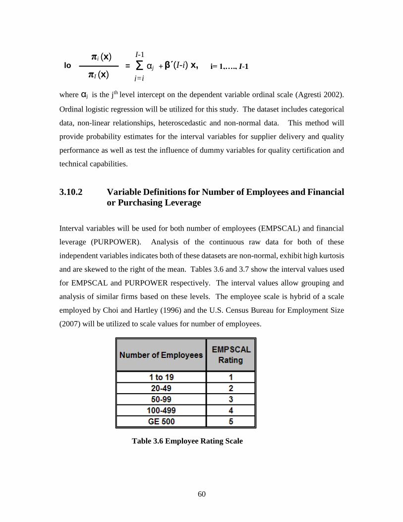
60
where αj is the jth level intercept on the dependent variable ordinal scale (Agresti 2002).
Ordinal logistic regression will be utilized for this study. The dataset includes categorical
data, non-linear relationships, heteroscedastic and non-normal data. This method will
provide probability estimates for the interval variables for supplier delivery and quality
performance as well as test the influence of dummy variables for quality certification and
technical capabilities.
3.10.2 Variable Definitions for Number of Employees and Financial
or Purchasing Leverage
Interval variables will be used for both number of employees (EMPSCAL) and financial
leverage (PURPOWER). Analysis of the continuous raw data for both of these
independent variables indicates both of these datasets are non-normal, exhibit high kurtosis
and are skewed to the right of the mean. Tables 3.6 and 3.7 show the interval values used
for EMPSCAL and PURPOWER respectively. The interval values allow grouping and
analysis of similar firms based on these levels. The employee scale is hybrid of a scale
employed by Choi and Hartley (1996) and the U.S. Census Bureau for Employment Size
(2007) will be utilized to scale values for number of employees.
= αj + log πI (x)
πi (x)
i= 1,…., I-1 Σ j=i
I-1
β΄(I-i) x,
Table 3.6 Employee Rating Scale

61
There are few research models which evaluate the effect of financial leverage or purchasing
power on supplier quality and delivery performance. Landry (1998) noted that a target of
20 to 40% of a supplier’s total revenue provided a power balance between the selling and
buying firms. The scale for financial leverage or purchasing power (shown in Table 3.7)
attempts to classify the various levels of the amount of business as a percentage of the total
company’s revenue. Ratings 1 and 2 on this scale represent relatively low levels of
business with the cutoff being 1% of total business for these classifications. A rating of 3
is assigned to a percentage of business which could certainly make the buying firm a top
100 customer. The rating of 4 represents a percentage of a supplier’s total revenue from 5
to 10 %, which would make the buying firm at least a top 20 customer. A rating of 5
represents between 10 and 20% of the supplier’s total revenues. At this level the customer
would at least be a top 10 customer and would approach the power balancing threshold
proposed by Landry. Level 6 represents suppliers in the power balancing range of above
20 % of total business levels. As noted by Dyer (1996) few of Chrysler’s suppliers relied
on Chrysler for the majority of their business while 16% of Toyota’s 310 suppliers relied
on Toyota for the majority of their business. Both the final leverage and employee scales
will be tested for their relationship with supplier delivery and quality performance.
Table 3.7 Financial Leverage or
Purchasing Leverage Rating Scale

62
3.10.3 Summary Statistics
Table 3.8 presents summary statistics for the variables used in this study. The sample size
for the independent variables ranged from 84 to 89 with a mean value of 87. Reviewing
the correlation coefficients shows a high degree of multicollinearity between the
independent variables. Multicollinearity occurs most frequently when independent
variables are defined using the same constructs (e.g., depression, anxiety) (Cohen et al.
2003). The objective of selection of the independent variables used in this study was
provide separate supplier attributes and test their relationship to supplier delivery and
quality performance.
The ordinal logistic regression model will test the heterogeneity of the independent
variables and their effects on the performance levels of the dependent variables quality and
delivery performance. It should be noted that the ordinal levels of the dependent variables
provide for improved testing of the strength of the association with the dependent variable’s
Table 3.8 Summary Statistics

63
levels and enhanced data analysis and output capabilities as compared to other logistic
regression models (Agresti 2002, Agresti 1984).
3.10.4 Model Definitions and Results
The model results for supplier quality and delivery performance versus various models will
presented in this section. Four models for each of the dependent variables were tested.
Model 1 (M1) represents the base line for testing of the supplier attributes versus the quality
organization certifications, quality technical capabilities, financial condition, supplier
payment performance, product differentiation and product complexity. This baseline
model presents a combination of independent variables that have been empirically tested
in conjunction with supplier performance. Other independent variables, such as financial
condition and supplier payment performance, and their relationship to supplier
performance have been hypothesized using deductive methods. The independent variable
product differentiation is included in the quality and delivery performance models. There
are no hypotheses, proposed in this research, which are associated with this variable.
Previous studies have tested the product differentiation and complexity pair versus supplier
performance. Therefore, in order to provide a consistent baseline model, the independent
variable product differentiation is included in Model 1. Model 2 (M2) adds the number of
employees to the baseline model. Model 3 (M3) adds the geographic location via the
mileage rating or distance variable. The distance variable is included in both the supplier
delivery and quality performance models, even though there is no specific hypothesis
included in the quality performance model for distance. Including the mileage rating in
both models facilitates consistent testing and presentation of results for both the supplier
quality and delivery performance models. Model 4 (M4) adds the financial power or
purchasing leverage to the final model.
The sample size of 82 meets the general approximation of 10 occurrences per predictor for
logistic regression (Agresti 2002). Tables 12 and 13 display the maximum likelihood
estimation results for the quality and delivery performance logits.

64
Table 3.9 provides summarized results for both the supplier quality and delivery models.
Reviewing the results for the supplier quality performance model testing, the χ2 and log-
likelihood diagnostic statistics are satisfactory for models M2 and M4 at a 5% significance
level while models M1 and M3 are significant at a 10% level. While the 5% significance
model is traditionally the cutoff used for presenting statistically significant results,
important information and relationships between supplier quality performance and key
attributes would be lost without including models M1 and M3. The following hypotheses
are rejected: H1 (Quality Organization Certification positively relates to improved
performance); H3 (Financial rating positively relates to performance); H4 (Supplier
Payment Performance positively relates to performance); H8 (Financial Leverage or
Purchasing Power will positively relate to performance). The following hypotheses are not
rejected: H2 (Quality Technical Capability will positively relate to performance); H5
(Product complexity will negatively relate to performance); H6 (Number of Employees will
negatively relate to performance). The financial leverage or purchasing power hypothesis
(H8) is rejected due to the unexpected negative relationship to quality. While the model
variable for financial leverage is reported to be significant at the 10% level, the negative
value for the coefficient does not support the a priori hypothesis.
The results for supplier delivery performance model testing reveal that all models (M1
through M4) are satisfactory for the χ2 and log-likelihood diagnostic statistics. The
following hypotheses are rejected: H1 (Quality Organization Certification positively relates
to improved performance); H2 (Quality Technical Capability will positively relate to
performance); H4 (Supplier Payment Performance positively relates to performance); H6
(Number of Employees will negatively relate to performance); H7 (Distance will negatively
relate to performance); H8 (Financial Leverage or Purchasing Power will positively relate
to performance). The following hypotheses are not rejected: H3 (Financial rating positively
relates to performance); H5 (Product complexity will negatively relate to performance).
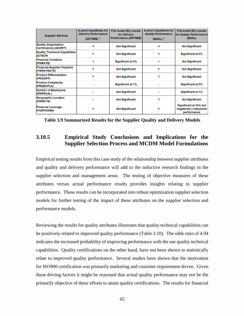
65
Table 3.9 Summarized Results for the Supplier Quality and Delivery Models
3.10.5 Empirical Study Conclusions and Implications for the
Supplier Selection Process and MCDM Model Formulations
Empirical testing results from this case study of the relationship between supplier attributes
and quality and delivery performance will add to the inductive research findings in the
supplier selection and management areas. The testing of objective measures of these
attributes versus actual performance results provides insights relating to supplier
performance. These results can be incorporated into robust optimization supplier selection
models for further testing of the impact of these attributes on the supplier selection and
performance models.
Reviewing the results for quality attributes illustrates that quality technical capabilities can
be positively related to improved quality performance (Table 3.10). The odds ratio of 4.94
indicates the increased probability of improving performance with the use quality technical
capabilities. Quality certifications on the other hand, have not been shown to statistically
relate to improved quality performance. Several studies have shown that the motivation
for ISO900 certification was primarily marketing and customer requirement driven. Given
these driving factors it might be reasoned that actual quality performance may not be the
primarily objective of these efforts to attain quality certifications. The results for financial

66
leverage or purchasing power while significant point out an interesting relationship. While
much has been written about the purchasing power, few studies have analyzed how the
level of business with a particular supplier might influence quality or delivery performance
(Table 3.11). James A. Wier, CEO of Simplicity Manufacturing, a lawn-mower maker that
decided to stop selling to Wal-Mart. "When you drive the cost of a product down, you
really can't deliver the high-quality product like we have (Bianco et al. 2003)”. It might be
expected that as financial leverage increases likewise it could be reasoned that quality and
delivery results would improve since that supplier is more and more dependent on the
customer for sales and revenue. Instead this model indicates that there is a significant
negative relationship between increasing business levels and quality performance. While
this is a surprising result, it could be inferred that as the amount of business increases with
a single customer, cost pressures, clearly described by Mr. Wier, could cause suppliers to
revise processes or cut costs resulting in reduced quality levels.
Product complexity is significant in both the quality and delivery models. Increasing
product complexity is related to decreasing supplier performance. Defect opportunities
increase for complex products, providing an interesting argument that as products becomes
increasingly complex the overall quality and delivery performance degrades. Financial
rating was also found to significantly relate to delivery performance. It has been deduced
that a healthy financial rating allows supplier flexibilities to meet changing requirements
such as a need for overtime and facility and equipment improvements. Without a healthy
financial rating, researchers have conjectured that supplier performance would be
degraded. This case study supports these assertions that a financially healthy company
provides improved delivery performance as compared to companies with poor financial
ratings. Dun and Bradstreet provides alerts to its subscribers notifying them when a
company’s financial rating changes in order to make them aware of possible supplier
performance problems.

67
Va
ria
ble
βi
SE
Co
eff
.
Od
ds
Ra
tio
βi
SE
Co
eff
.
Od
ds
Ra
tio
βi
SE
Co
eff
.
Od
ds
Ra
tio
βi
SE
Co
eff
.
Od
ds
Ra
tio
Co
ns
tan
t(1
)0.3
03
1.2
54
0.8
58
1.3
16
0.6
99
1.3
37
2.2
19
1.5
66
Co
ns
tan
t(2
)1.1
04
1.2
61
1.6
82
1.3
27
1.5
34
1.3
47
3.0
92
***
1.5
85
Co
ns
tan
t(3
)1.3
58
1.2
64
1.9
53
1.3
32
1.8
05
1.3
51
3.3
71
**1.5
92
QC
ER
T-0
.30
98
0.6
43
0.7
3-0
.13
18
0.6
743
0.8
8-0
.12
47
0.6
798
0.8
8-0
.23
30.6
944
0.7
9
QT
EC
H0.8
25
0.8
764
2.2
81.1
121
0.9
084
3.0
41.1
627
0.9
091
3.2
1.5
969
**0.9
488
4.9
4
FIN
RA
TE
0.3
687
0.3
096
1.4
50.3
983
0.3
177
1.4
90.3
795
0.3
192
1.4
60.3
43
0.3
263
1.4
1
FIN
PA
YR
AT
E0.1
046
0.4
009
1.1
1-0
.06
47
0.4
168
0.9
4-0
.04
76
0.4
205
0.9
5-0
.19
48
0.4
368
0.8
2
PR
OD
IFF
0.2
46
0.2
759
1.2
80.4
324
0.2
916
1.5
40.4
664
0.2
956
1.5
90.4
422
0.3
026
1.5
6
PR
OD
CP
LX
-0.7
837
**0.3
138
0.4
6-0
.38
64
**0.3
152
0.4
5-0
.82
03
**0.3
164
0.4
4-0
.66
69
**0.3
278
0.5
1
EM
PS
CA
L
-0
.38
64
***
0.2
142
0.4
5-0
.45
89
**0.2
311
0.6
3-0
.73
79
*0.2
758
0.4
8
DIS
RA
TE
0.1
472
0.1
807
1.1
60.0
478
0.1
924
1.0
5
PU
RP
OW
ER
-0.3
527
***
0.1
843
0.7
Lo
g-l
ike
lih
oo
d-8
9.1
28
-87.4
15
-87.1
08
-85.1
25
P-V
alu
e1
0.0
98
0.0
49
0.0
64
0.0
28
1T
he
P-V
alu
e i
s t
esti
ng
th
e jo
int
hyp
oth
esis
th
at
the
co
eff
icie
nts
are
eq
ua
l to
ze
ro.
M1 E
sti
ma
tes
Qu
ality
Va
ria
ble
s
Fin
an
cia
l V
ari
ab
les
Dis
tan
ce V
ari
ab
le
Pu
rch
as
ing
Po
we
r V
ari
ab
le
No
tes:
Pro
du
ct
Co
mp
lexit
y a
nd
Dif
fere
nti
ati
on
Va
ria
ble
s
*
sig
nif
ican
t @
1%
**
sig
nif
ican
t @
5%
***
sig
nif
ican
t @
10%
M2 E
sti
ma
tes
Op
era
tio
ns
Sc
ale
Va
ria
ble
M3 E
sti
ma
tes
M4 E
sti
ma
tes
Tab
le 3
.10 O
rdin
al
Logis
tic
Reg
res
sion
Res
ult
s fo
r S
up
pli
er Q
uali
ty P
erfo
rman
ce

68
Va
ria
ble
βi
SE
Co
eff
.
Od
ds
Ra
tio
βi
SE
Co
eff
.
Od
ds
Ra
tio
βi
SE
Co
eff
.
Od
ds
Ra
tio
βi
SE
Co
eff
.
Od
ds
Ra
tio
Co
ns
tan
t(1
)1.5
12
1.3
53
1.5
53
1.4
08
1.0
47
1.4
28
2.2
45
1.6
32
Co
ns
tan
t(2
)2.7
46
**1.3
70
2.7
86
***
1.4
26
2.2
95
1.4
43
3.5
31
**1.6
58
Co
ns
tan
t(3
)3.3
52
**1.3
86
3.3
92
**1.4
41
2.9
12
**1.4
57
4.1
73
**1.6
78
QC
ER
T0.0
112
0.6
211
1.0
10.0
308
0.6
419
1.0
30.0
618
0.6
484
1.0
60.0
092
0.6
498
1.0
1
QT
EC
H0.3
825
0.8
481
1.4
70.3
812
0.8
535
1.4
60.4
318
0.8
538
1.5
40.6
347
0.8
652
1.8
9
FIN
RA
TE
0.7
942
**0.3
271
2.2
10.7
922
**0.3
272
2.2
10.7
907
**0.3
296
2.2
00.6
627
**0.3
293
1.9
4
FIN
PA
YR
AT
E-0
.68
42
0.4
370
0.5
0-0
.69
19
0.4
508
0.5
0-0
.59
70.4
584
0.5
5-0
.64
01
0.4
651
0.5
3
PR
OD
IFF
0.4
391
0.2
958
1.5
50.4
475
0.3
061
1.5
60.4
538
0.3
062
1.5
70.4
239
0.3
092
1.5
3
PR
OD
CP
LX
-1.5
092
*0.3
648
0.2
2-1
.50
63
***
0.3
655
0.2
2-1
.54
03
*0.3
692
0.2
1-1
.41
48
*0.3
724
0.2
4
EM
PS
CA
L
-0
.02
25
0.2
188
0.9
8-0
.11
69
0.2
314
0.8
9-0
.28
63
0.2
603
0.7
5
DIS
RA
TE
0.2
723
0.1
827
1.3
10.1
937
0.1
902
1.2
1
PU
RP
OW
ER
-0.2
834
0.1
815
0.7
5
Lo
g-l
ike
lih
oo
d-9
0.9
50
-90.9
45
-89.7
08
-88.3
7
P-V
alu
e1
0.0
00
0.0
00
0.0
00
0.0
00
1T
he
P-V
alu
e i
s t
esti
ng
th
e jo
int
hyp
oth
esis
th
at
the
co
eff
icie
nts
are
eq
ua
l to
ze
ro.
No
tes:
*
sig
nif
ican
t @
1%
**
sig
nif
ican
t @
5%
Dis
tan
ce V
ari
ab
le
Pro
du
ct
Co
mp
lexit
y a
nd
Dif
fere
nti
ati
on
Va
ria
ble
s
***
sig
nif
ican
t @
10%
Pu
rch
as
ing
Po
we
r V
ari
ab
le
Op
era
tio
ns
Sc
ale
Va
ria
ble
Fin
an
cia
l V
ari
ab
les
Qu
ality
Va
ria
ble
s
M1 E
sti
ma
tes
M2 E
sti
ma
tes
M3 E
sti
ma
tes
M4 E
sti
ma
tes
Tab
le 3
.11 O
rdin
al
Logis
tic
Reg
res
sion
Res
ult
s fo
r S
up
pli
er D
eliv
ery P
erfo
rman
ce

69
While these results provide some interesting insights into attributes often included as part
of the supplier selection processes, clearly a great deal of research is required to add to this
important body of knowledge. This study presents a method for further investigation of
this critical process. The motivation for this examination of critical supplier attributes and
supplier delivery and quality performance was to utilize these results into an integrated
supplier selection model with product life cycle considerations. This integrated supplier
selection model and a real world case study will be presented in the following chapters.

70
4. General Model for Supplier Selection incorporating results
of Empirical Study and Product Life Cycle
This chapter will present a supplier selection model which incorporates both the findings
from the empirical model presented in Chapter 3 and product life cycle considerations. An
illustrative example, as well as a case study using industrial data, will be developed
using a number of goal programming solution approaches including: preemptive GP; non-
preemptive GP; Tchebycheff (Min-Max) GP and Fuzzy GP.
This model is intended for selecting suppliers who have been short-listed. This is typically
the second phase of the supplier selection where the final supplier selections are completed
using the decision maker’s criteria. The major distinguishing features of this general model
include the following:
1. Integration of the product life cycle into the supplier selection model, through the
inclusion of items representing the introduction, growth, maturity and decline
phases of the product life cycle.
2. Inclusion of model parameters, based on the results of the empirical study of key
supplier attributes versus supplier performance, including: the maximum amount
of business allowed for a particular supplier; the financial condition of a supplier,
the minimum allowed financial condition required for a supplier of a particular
item, the quality technical capability of the supplier and the minimum required
quality technical capability required for a supplier of a particular item.

71
3. The objectives of the supplier selection model include minimization of cost, lead-
time, quality defects and late deliveries.
4. In addition to the capacity constraints, the model includes constraints on the
maximum amount of business which can be placed on particular suppliers.
Additionally, the financial condition of a supplier is included as a constraint
insuring the supplier meets the minimum requirements for financial stability
required to supply an item in a specific stage of the product life cycle. Similarly, a
minimum quality technical capability of a supplier is included as a constraint
insuring the supplier meets the minimum requirements for quality technical
capability required to supply an item in a specific stage of the product life cycle. A
demand constraint is included in the model as well. The maximum and minimum
number of suppliers’ constraints for a particular item are also included as
constraints. These constraints will be varied based on the item’s stage in the
product life cycle. For example, multiple sourcing may be required for critical
products in the introduction stage while single sourcing may be employed for
products in the decline stage of the product life cycle. The amount of business
constraint, financial condition, quality technical capability constraints are
included in the general model based on the results from the empirical study.
4.1 Notations used in the model
Model Indices
I = Set of products to be purchased, which can be in any one of the different mutually
exclusive stages of product life cycle. The product life cycle includes Introduction
(I1), Growth (I2), Maturity (I3) and Decline (I4), i.e. 4321
IIIII = .

72
K Potential set of suppliers
Model Parameters
pik Cost of acquiring one unit of product i from supplier k
Fk Fixed ordering cost associated with purchasing any product from supplier k
Gik Tooling cost associated with acquiring product i from supplier k
di Demand of product i
lik Lead time of supplier k to produce and supply product i
qik Quality that supplier k maintains for product i, which is measured as percent yield
delik Delivery performance that supplier k provides for product i, which is measured as
percent on-time deliveries
mbk Maximum amount of business ($) for a particular supplier k for a given planning
horizon
finck The financial condition of a supplier k
rfinci The required minimum financial condition for a supplier to supply product i
qtk The quality technical capability of supplier k
rqti The required quality technical capability for a supplier to supply product i
CAPik Production capacity for supplier k for product i
Mi Maximum number of suppliers that can be selected for product i
Ni Minimum number of suppliers that should be selected for product i (e.g. multiple
sources for critical product or critical phase of product life cycle).

73
Decision Variables in the model
Xik Number of units of product i supplied by supplier k
δik Binary variable denoting if a particular supplier is chosen or not for product i. This
is a binary variable which takes a value 1 if a supplier is chosen to supply product
i and is zero, if the supplier is not chosen.
4.2 Mathematical Formulation of the Order Allocation Problem
4.2.1 Objective Functions
The four conflicting objectives used in the model are minimization of cost, lead-time,
rejects and delivery delays. It is relatively easy to add other objectives also. The
mathematical forms for these objectives are given below:
1. Procurement Cost (Z1n): Total cost of purchasing has two components; fixed and
the variable cost.
Total variable cost: The total variable cost is the cost of buying every additional
unit from the suppliers for each of the four phases of the product life cycle (Z1n for
n = 1,..,4) which represent the four phases of the product life cycle. At a specific
point in time each product i is known to be in a particular stage of the product life
cycle (introduction (I1), growth (I2), maturity (I3) and decline (I4)) and the variable
costs are assumed to be known. The total variable cost objective function is given
by:
ik
Ii k
ik Xpn
for n = 1, 2, 3, 4.

74
Fixed Costs: If a supplier k is used for product i, then there are fixed costs associated
with utilizing supplier k, as well as tooling costs associated with product i being
supplied by supplier k. The total fixed cost is given by:
k
ikkF + k
ikik
Ii
Gn
for n = 1, 2, 3, 4.
Where Fk is the fixed cost of using supplier k and Gik is the fixed tooling cost of
supplier k for supplying product i.
Hence the total Cost (Z1n) is
++
n
n n
Ii k
ik
Ii k k Ii k
ikikikkikik
X
GFXp
for n = 1, 2, 3, 4. (4.1)
In equation (4.1), the objectives Z1n (n = 1,..,4) correspond to the weighted
procurement costs of all products and suppliers in the life cycle phase n. The
denominator, which represents the sum of all demands for products in phase n, is a
constant and can be ignored in the optimization process. This results in linear
objective functions for the procurement cost corresponding to each product life
cycle phase. At any time, each product i is known to be in a particular stage of the
product life cycle (introduction (I1), growth (I2), maturity (I3) and decline (I4)) and
the value of the procurement costs are assumed to be known.
2. General Lead-time (Z2n):
n
n
Ii k
ik
Ii k
ikik
X
Xl
for n = 1, 2, 3, 4. (4.2)
Similarly the general lead-time objective is partitioned into four lead-time
objectives, Z21, Z22, Z23 and Z24, which correspond to the four phases of the product
life cycle. The lead-time objective function Z21 relates to products in the

75
introductory stage; Z22 relates to products in the growth stage; Z23 relates to
products in the maturity phase and Z24 relates to products in the decline phase. The
objectives Z2n (n = 1,2,..,4) correspond to the weighted lead-times of all products
and suppliers in life cycle phase n. The denominator, which represents the sum of
all demands for products in phase n, is a constant and can be ignored in the
optimization process. Hence, the general lead-time objectives (Eq. 4.2) are also
linear functions.
At any time, each product i is known to be in a particular stage of the product life
cycle (introduction (I1), growth (I2), maturity (I3) and decline (I4)) and the values of
the lead-times are also assumed to be known.
3. General Quality (Z3n):
n
n
Ii k
ik
Ii k
ikik
X
Xq
for n = 1, 2, 3, 4. (4.3)
The general quality objective is likewise partitioned into four quality objectives
(Z3n for n = 1,..,4), which correspond to the four phases of the product life cycle.
The objective Z3n corresponds to the weighted quality performance, based on
product reject rates, for all products and suppliers in phase n. The denominator,
which is identical to the denominator in the cost and lead-time objectives, also
represents the sum of all demands for the products in phase n, which is a constant
and can be ignored in the optimization process. Thus, the quality objectives (Eq.
4.3) are also linear functions.

76
4. General Delivery (Z4n):
n
n
Ii k
ik
Ii k
ikik
X
Xdel
for n = 1, 2, 3, 4. (4.4)
The general delivery objective is also partitioned into four delivery objectives (Z4n
for n = 1,..,4), which correspond to the four phases of the product life cycle. The
objective Z4n corresponds to the weighted delivery performance, measured in terms
of late deliveries, for all products and suppliers in phase n. The denominator is
utilized to represent the sum of all demands, which is a constant and can be ignored
in the optimization process. Thus, the delivery objectives are also linear functions
(Eq. 4.4).
Thus, we have 16 objective functions in the optimization model, four for each
product life cycle phase.
4.2.2 Constraints
The constraints in the model are as follows:
1. Capacity constraints: Each supplier k has a maximum capacity for product i,
CAPik. Total order placed with this supplier must be less than or equal to the
maximum capacity for product i. The capacity constraint is varied by product given
that a supplier’s capacity may vary by product. Hence the capacity constraint is
given by:
ikik
i
ik CAPX )( i,k.. (4.5)
The binary variable on the right hand side of the constraint implies that supplier k
cannot supply product i if they are not chosen, i.e., if δik is 0.

77
2. Business Volume Constraints: The total business volume for a set of products i
received from supplier k must be less than the maximum amount of business level
for the supplier. The business volume constraint for each supplier is given by:
kik
iik
mbXp k . (4.6)
3. Financial Condition Constraints: The minimum financial condition required to
do business for product i with supplier k is given by:
irfinc
ikkfinc ki, . (4.7)
4. Quality Technical Capability Constraints: Denotes the quality technical
capability condition for product i required to do business with a supplier k. They
are given by:
irqt
ikkqt ki, . (4.8)
5. Demand Constraints: The demand for product i has to be satisfied using a
combination of the suppliers. The demand constraints are given by:
idXi
kik
= . (4.9)
6. Maximum number of suppliers: The maximum number of suppliers chosen for
product i must be less than or equal to a specified number. It is given by:
k
iik M .
(4.10)
Where Mi is the specified maximum for product i.
7. Minimum number of suppliers: The minimum number of suppliers chosen for
product i must be greater than or equal to a specified number. It is given by:

78
k
iik N . Where Ni, is the specified minimum for product i. (4.11)
Note: If iN 2 then multiple sourcing is enforced.
8. Non- Negativity and Binary constraints:
(0,1) ;0X ikik . (4.12)
4.3 Goal Programming (GP) Models
Goal programming will be used to solve the multiple objective linear integer program
developed in Section 4.2. This section will briefly explain the ideal solutions, goal
constraints, formulation and objectives of the preemptive and non-preemptive goal
programming models as well as the formulation of the Tchebycheff’s min-max and Fuzzy
GP models.
Goal programming utilizes target levels for the achievement of the objective functions,
represented by equations 4.1 to 4.4. These GP objectives are assigned target levels and
priorities for achieving the stated targets. These target values are treated as goals to strive
for. Since not all the targets may be achievable, deviational variables are used to allow for
the under or overachievement of the targets. The target levels are established by first
determining the ideal solutions. Generation of the ideal solutions will be discussed next.
4.3.1 Ideal Solutions
The initial step required prior to solving the problem using the various goal programming
models is to obtain the ideal values, which will be used by all of the GP models. Ideal
values are the best values achievable for each objective, ignoring the other objectives. In
this case, single objective optimization models are created for the four objectives of quality,
delivery, cost and lead-time for each of the four products, yielding sixteen individual linear
integer programs, in order to determine the ideal values. The ideal values are calculated
by individually solving these sixteen linear programs, one for each of the objectives and

79
for each of the four products and their respective phases in the product life cycle. The ideal
values will then be utilized to set target values for the various goal programming models.
4.3.2 General Goal Programming Model
The multi-objective problem using goal programming is created by partitioning each of the
four objectives: cost (4.1), lead-time (4.2), quality (4.3) and delivery (4.4) into the four
phases of the product life cycle and their respective goal constraints. First the cost objective
will be explained.
The general cost objective (4.1) is partitioned into four cost objectives, Z11, Z12, Z13 and
Z14, which correspond to the four phases of the product life cycle. The objective function
Z11 relates to procurement cost in the introductory phase; Z12 relates to procurement cost
in the growth phase; Z13 relates to procurement cost in the maturity phase and Z14 relates
to procurement cost in the decline phase. Each of the four cost objectives have target
values, denoted by T1n (n = 1,..,4), for each of the product life cycle phases. At any
particular point in time each product i is known to be in a particular stage of the product
life cycle (introduction (I1), growth (I2), maturity (I3) and decline (I4)) and the values of the
fixed and variable costs are known.
T11 relates to the objective function Z11 and the introductory phase; T12 relates to the
objective function Z12 and the growth phase; T13 relates to the objective function Z13 and
the maturity phase and T14 relates to the objective function Z14 and the decline phase.
Deviational variables d1n- and d1n
+, (n = 1,..,4) for each of the product life cycle phases, are
also included in the objective function. The deviational variables allow the under (d1n-) or
overachievement (d1n+) of the goal constraints. Given the objective is to minimize cost,
the goal is to minimize the positive deviational variable d1n+ (n = 1,..,4) for each of the
product life cycle phases.
The cost goal constraints are given below:
Z11 (Intro. phase) =
++1 1
iiiiIi k k Ii k
kkkkkki GFXp + d11- - d11
+ = T11; (4.13)

80
Z12 (Growth phase) =
++2 2
iiiiIi k k Ii k
kkkkkki GFXp + d12- - d12
+ = T12; (4.14)
Z13 (Maturity phase) =
++3 3
iiiiIi k k Ii k
kkkkkki GFXp + d13- - d13
+ = T13;
(4.15)
Z14 (Decline phase) =
++4 4
iiiiIi k k Ii k
kkkkkki GFXp + d14- - d14
+ = T14. (4.16)
Like the cost objectives, each of the four lead-time objectives have target values T2n (n =
1,..,4) for each of the product life cycle phases. T21 relates to the objective function Z21
and the introductory phase; T22 relates to the objective function Z22 and the growth phase;
T23 relates to the objective function Z23 and the maturity phase and T24 relates to the
objective function Z24 and the decline phase. Deviational variables d2n- and d2n
+, (n = 1,..,4)
are included to allow the underachievement (d2n-) or overachievement (d2n
+) of the goal
constraints for the product life cycle phases. Given the objective is to minimize lead-time,
the goal is to minimize the positive deviational variable d2n+ (n = 1,..,4) for each of the
product life cycle phases.
The lead-time goal constraints are given below:
Z21 (Introduction phase) =
1Ii k
ikik Xl + d21- - d21
+ = T21; (4.17)
Z22 (Growth phase) =
2Ii k
ikik Xl + d22- - d22
+ = T22; (4.18)
Z23 (Maturity phase) =
3Ii k
ikik Xl + d23- - d23
+ = T23; (4.19)
Z24 (Decline phase) =
4Ii k
ikik Xl + d24- - d24
+ = T24. (4.20)
Similar to the cost and lead-time objectives, each of the four quality objectives have target
values T3n (n = 1,..,4) for each of the product life cycle phases. T31 relates to the objective
function Z31 and the introductory phase; T32 relates to the objective function Z32 and the
growth phase; T33 relates to the objective function Z33 and the maturity phase and T34
relates to the objective function Z34 and the decline phase. Deviational variables d3n- and

81
d3n+, (n = 1,..,4), corresponding to the product life cycle phases, are included allowing the
underachievement (d3n-) or overachievement (d3n
+) of the goal constraints. Given the
objective is to maximize quality performance, the goal is to minimize the negative
deviational variable d3n- (n = 1,..,4) for each of the product life cycle phases.
The quality goal constraints are given below:
Z31 (Introduction phase) =
1Ii k
ikik Xq + d31- - d31
+ = T31; (4.21)
Z32 (Growth phase) =
2Ii k
ikik Xq + d32- - d32
+ = T32; (4.22)
Z33 (Maturity phase) =
3Ii k
ikik Xq + d33- - d33
+ = T33; (4.23)
Z34 (Decline phase) =
4Ii k
ikik Xq + d34- - d34
+ = T34. (4.24)
In the same manner as the previously detailed objectives, the four delivery objectives have
target values T4n (n = 1,..,4) for each of the product life cycle phases. T41 relates to the
objective function Z41 and the introductory phase; T42 relates to the objective function Z42
and the growth phase; T43 relates to the objective function Z43 and the maturity phase and
T44 relates to the objective function Z44 and the decline phase. Deviational variables d4n-
and d4n+, (n = 1,..,4), relating to the product life cycle phases, are incorporated in the
objective function allowing the underachievement (d4n-) or overachievement (d4n
+) of the
goal constraints. Given the objective is to maximize delivery performance, the goal is to
minimize the negative deviational variable d4n- (n = 1,..,4) for each of the product life cycle
phases.
The delivery goal constraints are given below:
Z41 (Introduction phase) =
1Ii k
ikik Xdel + d41- - d41
+ = T41; (4.25)
Z42 (Growth phase) =
2Ii k
ikik Xdel + d42- - d42
+ = T42; (4.26)
Z43 (Maturity phase) =
3Ii k
ikik Xdel + d43- - d43
+ = T43; (4.27)

82
Z43 (Decline phase) =
4Ii k
ikik Xdel + d44- - d44
+ = T44. (4.28)
Thus we have 16 goal constraints in this optimization model. The real constraints, which
are given by equations 4.5 to 4.12, represent the boundaries of the decision space for the
objectives and decision variables for all the GP models.
After setting the target levels for the goal constraints, the relative importance of achieving
the targets have to be specified. Different goal programming models are used to specify
the relative importance. These GP models include preemptive, non-preemptive,
Tchebycheff’s min-max and Fuzzy methods. A brief discussion of the GP models and the
application to solving the general model follows.
4.3.3 Preemptive Goal Programming Model
Preemptive GP requires the decision maker to identify the order in which goal constraints
will be achieved after setting the target levels (T11 to T44) for goal constraints. This requires
the decision maker to rank order the goal constraints (equations 4.13 to 4.28) from highest
to lowest priority. Priority order of the goal constraints is determined by the decision maker
(DM). No scaling of the goal constraints is required since higher goal constraint
achievement supersedes the attainment of the lower priority goal constraints. Therefore
preemptive GP does not require a great deal of cognitive effort by the DM since they are
simply ranking the goal constraints in priority order sequence and setting target levels. A
pair-wise comparison method can be used to get the rankings of the goals.
The target levels for the preemptive GP model are set using the ideal solutions, which
were determined by solving for the ideal values described in Section 4.3.1. For
illustration, the target levels are set at 90% of the ideal values for maximization, such as
quality and delivery performance. Target levels for cost and lead-time are set at 110% of
the ideal values given the objective of minimizing these goal constraints. Decision
makers ultimately will set the appropriate target levels. Setting the targets at 90% and

83
110% for maximization and minimization goal constraints for the illustrative example
allows for consistent comparisons among the various GP model results.
4.3.4 Non-preemptive Goal Programming Model
Non-preemptive GP requires the DM to determine the relative weights in achieving the
targets (T11 to T44) for the goal constraints. The goal constraints, deviational variables and
targets, given in equations 4.13 to 4.28, along with the real constraints, given in equations
4.5 to 4.12, are used in a single objective model. The relative weights (win) are set for each
of the deviational variables (din) in the single objective model. Similar to the preemptive
GP method, the target levels are set at 90% of the ideal values for the quality and delivery
objectives. Likewise the cost and lead-time minimization objectives are set at 110% of the
ideal values.
The Borda Count method or Analytic Hierarchy Process can be utilized by the DM to
determine the relative weights of the goal constraints. This increases the cognitive burden
on the DM given the 16 goal constraints. Scaling or normalization of the goal constraints
is also required to facilitate an equitable comparison among the objectives.
4.3.5 Tchebycheff’s Min-Max Goal Programming Model
The Tchebycheff’s goal programming methodology also uses goals/targets for each of the
objectives and deviational variables to represent violations from the targets, but it does not
use priorities or weights for the goals. Instead, it minimizes the maximum deviation from
the targets (T11 to T44), using the deviational variables (d11 to d44). Tchebycheff’s min-max
GP requires the decision maker to determine the targets for the goal constraints. The goal
constraints, deviational variables and targets, given in equations 4.13 to 4.28, along with
the real constraints, given in equations 4.5 to 4.12, are used in a single objective model.
The target levels, for the illustrative example, are set at 90% of the ideal values for the
maximization goal constraints for quality and delivery. The cost and lead-time
84
minimization objectives are set at 110% of the ideal values. This target level setting places
minimal analytical requirements on the DM. Scaling of the goal constraints is required.
4.3.6 Fuzzy Goal Programming Model
The Fuzzy GP model does not use targets for the objectives. Instead, it uses the ideal values
as the targets. Similar to the Tchebycheff GP model, it minimizes the maximum deviation
from the ideal values. Thus, Fuzzy GP neither requires target levels nor preferences among
the targets.
4.4 Illustrative Example
A realistic example problem is created to demonstrate the application of the goal
programming models. The example includes four products selected from the introduction,
growth, mature and decline stages of the product life cycle and five suppliers. The
suppliers have varying performance levels for cost, lead-time, quality and delivery. Table
4.1 presents the supplier data by product life cycle phase. For the illustrative example, we
have excluded the fixed costs of using a supplier. The fixed tooling costs are included in
the example. Results for the various GP models will be discussed in the following sections
ending with an overall summary comparing the results of all the models. The first step is
to determine the ideal solutions, which will be discussed in the following section.
4.4.1 Ideal Solutions
The initial step in the GP model is to create and solve sixteen single objective linear integer
programs in order to determine the ideal values for the four objectives of cost, lead-time,
quality and delivery, for each of the four product life cycles.
Table 4.2 presents the optimal solutions for the sixteen single objective linear integer
programs. For example, the minimization of lead-time for the introduction product is

85
accomplished by first selecting supplier 5, who has the minimum lead-time of five weeks.
There is a capacity constraint on supplier 5 of 100 units, so it is necessary to choose a
second supplier in order to fulfill the demand requirement of 120 units. Supplier 1 is then
Table 4.1 Supplier Data for Illustrative Example

86
chosen to fulfill the remaining demand of 20 units since it has the next lowest lead-time at
6 weeks. The process continues for the introduction product, with suppliers being chosen
to maximize delivery and quality performance, and minimize cost. These are relatively
straightforward selections with the choice of the supplier with the best quality and delivery
performance and lowest overall cost.
The growth product requires a minimum selection of two suppliers to fulfill the demand of
230 units. Suppliers 2 and 4 have equivalent performance for lead-time and delivery at 6
weeks and 99% on-time delivery performance. The optimization software selects supplier
Table 4.2 Ideal Solutions for the Illustrative Example

87
2 for 220 units and supplier 4 for 10 units in order to fulfill the two supplier minimum as
well as the minimum order quantity of 10 units for supplier 4.
Similarly, the mature product’s constraints require the selection of two suppliers to fulfill
the demand of 390 units. The cost objective is met by ordering 380 units from supplier 3,
who has the overall minimum total cost, and 10 units from supplier 1, who has the next
lowest total overall cost. Supplier 2 is chosen for lead-time and delivery ordering 200 units
from supplier 2 and 190 units from supplier 3. Supplier 2 has a capacity constraint of 200
units. Even though it has the best performance for lead-time and delivery, an additional
190 units must be ordered from supplier 3, which has the second best performance for both
of these objectives.
The decline product selections are relatively straightforward with supplier assignments for
both delivery and quality being made from the best performing suppliers. Supplier 3 is
selected for the minimum lead-time at 10 weeks, but a capacity constraint of 80 units
requires the selection of supplier 2, which has the second lowest lead-time at 12 weeks.
Similarly Supplier 3 has the lowest cost but due to the capacity constraint, supplier 1 is
selected to fulfill the remaining 20 units.
The ideal solutions are now used to set target levels for the preemptive, non-preemptive
and Tchebycheff min-max models. The preemptive GP results are discussed in the next
section.
4.4.2 Preemptive Goal Programming Results
In preemptive goal programming, the decision maker (DM) identifies the order in which
goal constraints will be achieved after setting the target levels (T11 to T44) for the goals.
For illustrative purposes, the target levels are set at 90% of the ideal values for
maximization and 110% of the ideal values for minimization for the four objectives (cost,
lead-time, quality and delivery) and for each of the four products and their respective phase
in the product life cycle. This relaxing of target values provides some flexibility with
respect to attaining the conflicting goals. Next the DM rank orders the goal constraints
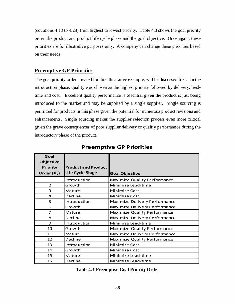
88
(equations 4.13 to 4.28) from highest to lowest priority. Table 4.3 shows the goal priority
order, the product and product life cycle phase and the goal objective. Once again, these
priorities are for illustrative purposes only. A company can change these priorities based
on their needs.
Preemptive GP Priorities
The goal priority order, created for this illustrative example, will be discussed first. In the
introduction phase, quality was chosen as the highest priority followed by delivery, lead-
time and cost. Excellent quality performance is essential given the product is just being
introduced to the market and may be supplied by a single supplier. Single sourcing is
permitted for products in this phase given the potential for numerous product revisions and
enhancements. Single sourcing makes the supplier selection process even more critical
given the grave consequences of poor supplier delivery or quality performance during the
introductory phase of the product.
Table 4.3 Preemptive Goal Priority Order
Goal
Objective
Priority
Order (P i )
Product and Product
Life Cycle Stage Goal Objective
1 Introduction Maximize Quality Performance
2 Growth Minimize Lead-time
3 Mature Minimize Cost
4 Decline Minimize Cost
5 Introduction Maximize Delivery Performance
6 Growth Maximize Delivery Performance
7 Mature Maximize Quality Performance
8 Decline Maximize Delivery Performance
9 Introduction Minimize Lead-time
10 Growth Maximize Quality Performance
11 Mature Maximize Delivery Performance
12 Decline Maximize Quality Performance
13 Introduction Minimize Cost
14 Growth Minimize Cost
15 Mature Minimize Lead-time
16 Decline Minimize Lead-time
Preemptive GP Priorities

89
For the growth phase, lead-time is given the highest priority, followed by delivery, quality
and cost respectively. Minimizing lead-time is critical given an increasing product volume
in order to meet customer demand during this ramp-up period. The supply chain must be
responsive during the introduction and growth phases of the product life cycle as opposed
to being cost efficient (Fisher 1997). Since there are fewer competitors and the profit
margins of products in these phases of the product life cycle are generally higher, supply
chain responsiveness in the form of shortened lead-times and excellent delivery
performance is critical. Delivery performance is closely related to lead-time and is the
second highest priority. The real constraints require the selection of two or more suppliers
in order to provide alternative sources as a hedge against possible supplier quality or
delivery performance problems.
In the mature phase, cost is the highest priority for items in this phase of the product life
cycle (PLC) followed by quality, delivery and lead-time. Given the competitive nature of
products in the maturity phase of the PLC, cost is the key factor required to maintain a
competitive position. Quality performance must remain high and is ranked second.
Delivery and lead-time are assigned lower priorities, given that mature products should
have smaller variations in demand which in turn cause fewer supply chain disruptions. The
supply chain, like the products in this phase, should be well established, cost efficient and
capable of supplying products without delivery and lead-time problems. The real
constraints require the selection of two or more suppliers for this phase of the PLC, which
provides some backup in case one of the supplier’s performance falters, as well as ensures
an on-going price competition between several suppliers.
Like the mature phase, cost is the highest priority for items in the decline phase of the PLC
followed by delivery, quality and lead-time. Cost is the key factor for products in the
decline phase, given the availability of competing products and profit margins are low.
Products must be available to the customer and therefore delivery is ranked as the second
highest priority. Products in this phase of the PLC can be easily substituted. Therefore
delivery performance is a key factor in the supplier selection process insuring product
availability. Products in this phase should have well established manufacturing and quality

90
control processes. Since cost is a key factor, efficient supplier performance with respect
to productivity and overall product quality is a requirement to provide products in the
decline phase. Alternate supply sources should be available and can be utilized as needed
on short notice. Therefore the real constraint allows the selection of only one supplier for
a product in the decline phase of the PLC.
Preemptive GP Solution
The goal constraints, presented in equations 4.13 to 4.28, and the corresponding deviational
variables and real constraints, presented in equations 4.5 to 4.12, are solved sequentially
according to the priority sequence (Pi) shown in Table 4.3. This requires that the optimal
solution for priority 1, namely maximize quality performance for the introduction product,
be determined first. The achieved value for priority 1 is then inserted as a real constraint
into the priority 2 GP model in order to ensure that the achievement of priority 1 goal is
maintained during the solution of priority 2; hence the name preemptive goal programming.
Next the results for the first two goal programs are added to the third highest priority model,
which is to minimize the overall procurement cost for the mature product. These steps are
repeated until all 16 priorities are solved. This insures the achievement of the higher
priorities before the lower priority goals are even considered. Goal conflicts occur as goal
constraints are added for the lower priorities. The preemptive goal programming
methodology insures higher goals are maintained at the detriment of lower priority goals.
The preemptive GP method requires the decision maker to simply order the goal priorities
thereby greatly reducing the cognitive burden on the DM. Another advantage is that the
objectives/goals do not have to be scaled.
The illustrative example results for the preemptive goal program exceeded or achieved
fifteen of the sixteen targets. Only lead-time for the mature product missed the target value.
Table 4.4 presents the preemptive goal achievements and Table 4.5 presents the optimal
procurement plan. A quick examination of Table 4.4 shows targets being exceeded
between 4.90 and 11.11% with a median value of 8.48%. The relaxation of the target
values to 90% of the ideal values for maximization (quality and delivery performance) and

91
110% of the ideal values for minimization (cost and lead-time) clearly had a significant
impact on the final results and procurement plan. Next the results for each of the product
life cycle phases will be examined in detail.
Introduction Phase Results (Tables 4.4 and 4.5)
Examining the results for the introduction PLC phase reveals that the suppliers with the
best values for achieving the objectives are not always chosen. For example, supplier 2 has
the highest quality yield at 97%, but suppliers 1 and 5 are selected since their combined
performance exceeds the target value of 104.76, for quality, while simultaneously
exceeding the delivery, lead-time and cost target levels. While the introduction goal
constraints for quality (4.21) and delivery (4.25) have higher priority rankings than lead-
time, it is the lead-time goal constraint (4.17) which drives the selections of supplier 1 and
5 in the final procurement plan. Suppliers 5 and 1 have the lowest lead-time, with 5 and 6
weeks respectively, which dictates their selection. Finally the cost target is achieved using
the same selections as lead-time, bypassing supplier 3, which has the overall lowest cost in
terms of variable and fixed costs. Unfortunately supplier 3’s quality and lead-time
performance prevent its selection given the quality and lead-times are higher priorities and
take precedence.
Growth Phase Results (Tables 4.4 and 4.5)
The growth PLC phase has the lead-time goal constraint (4.18) as Priority 2 in the
preemptive GP model. Suppliers 2 and 4 are selected since they provide the minimum
lead-time of 6 weeks. The minimum number of supplier constraint (4.11) requires the
selection of at least 2 suppliers for growth product; hence the selection of suppliers 2 and
4. The delivery goal constraint (4.26), which is Priority 6 in this model, will also select
supplier 2 and 4. They have the highest on-time delivery at 99%, so there is no compromise
required with respect to achieving this priority. Next the quality goal constraint (4.22) will
require the selection of supplier 4 prior to supplier 2, since supplier 4’s quality exceeds that
of supplier 2. To complete the supplier selection process for the growth product, the order

92
allocation remains the same with suppliers 4 and 2 satisfying the cost goal constraint (4.14).
Examining the procurement plan for this product life cycle phase clearly demonstrates the
impact of the relaxation of the targets since all targets were met with no change in the
supplier selection following the delivery constraint solution. Supplier 4 was chosen for the
majority of the order quantity due to the superior quality performance as compared to
supplier 2.
Table 4.4 Preemptive GP Achievements with respect to Target Values
Product and
Product Life
Cycle Stage
Goal
Priority
Order Goal Constraints
Target Values
(90% or 110% of
Ideals)
Goal
Achievements Target Achievement
Introduction 1 Maximize Quality Performance 104.76 113.00 Exceeded by 7.87%
Introduction 5 Maximize Delivery Performance 105.84 112.00 Exceeded by 5.82%
Introduction 9 Minimize Lead-time 682.00 620.00 Exceeded by 9.09%
Introduction 13 Minimize Cost 25,300.00 25,300.00 Achieved Target
Growth 2 Minimize Lead-time 1,518.00 1,380.00 Exceeded by 9.09%
Growth 6 Maximize Delivery Performance 204.93 227.70 Exceeded by 11.11%
Growth 10 Maximize Quality Performance 202.77 222.60 Exceeded by 9.78%
Growth 14 Minimize Cost 89,375.00 85,000.00 Exceeded by 4.90%
Mature 3 Minimize Cost 106,095.00 96,450.00 Exceeded by 9.09%
Mature 7 Maximize Quality Performance 347.49 363.30 Exceeded by 4.55%
Mature 11 Maximize Delivery Performance 342.27 378.10 Exceeded by 10.47%
Mature 15 Minimize Lead-time 1,705.00 1,960.00 Missed by 14.96%
Decline 4 Minimize Cost 46,777.50 42,525.00 Exceeded by 9.09%
Decline 8 Maximize Delivery Performance 85.50 91.80 Exceeded by 7.37%
Decline 12 Maximize Quality Performance 89.10 94.80 Exceeded by 6.40%
Decline 16 Minimize Lead-time 1,144.00 1,100.00 Exceeded by 3.85%
Preemptive GP Model Results in Product Life Phase and Priority Sequence

93
Table 4.5 Preemptive GP Procurement Plan
Mature Phase Results (Tables 4.4 and 4.5)
In the mature PLC phase, the cost goal constraint (4.15), with priority 3 in the overall GP
model, actually achieves the ideal solution selecting the minimum cost suppliers.
Therefore this solution exceeds the relaxed targets, which in this case is set at 110% of the
ideal. The next priority (priority 7) is to maximize quality performance. Suppliers 1 and
3 are again selected matching the supplier selection for the cost constraint. While the other
supplier selections would improve the overall quality results, this selection still exceeds the
target. The lead-time goal constraint (4.19) target is missed by nearly 15%. This failure is
due to the priority ordering of the goals in the preemptive model with the higher priorities
taking precedence.
Decline Phase Results (Tables 4.4 and 4.5)
The decline phase of the PLC has cost as the top priority at priority 4 in the overall model.
Again the cost goal constraint (4.16) solution actually equals the ideal solution with the
selection of supplier 3, which has a capacity of 80 units, followed by the selection of
Product and Product Life Cycle Stage Supp
lier 1
Supp
lier 2
Supp
lier 3
Supp
lier 4
Supp
lier 5
Introduction1 20 0 0 0 100
Growth2 0 10 0 220 0
Mature3,4 10 0 380 0 -
Decline5 20 0 80 - -
2 Requires Minimum of two suppliers3 Requires Minimum of two suppliers and Maximum of three suppliers4 Supplier 1 capacity limit of 75, Supplier 3 capacity limit of 2005 Supplier 3 capacity limit of 80
Optimal Order Allocations to Suppliers
1 Supplier 5 capacity limit of 100
94
supplier 1 for the remaining 20 units. The relaxation of the cost goal target to 110% of the
ideal guarantees these selections will exceed the target. The delivery goal constraint (4.28)
exceeds the target value, which has been relaxed to 90% of the target. While supplier 1
has the best delivery performance at 95%, the selection of supplier 3 with a delivery
performance of 91% still allows the optimal solution to exceed the target value. Likewise,
the quality goal constraint (4.24) also exceeds the target value. Finally, the lead-time goal
constraint (4.20) is met primarily by the selection of supplier 3, which has the best lead-
time, for 80 of the 100 units required. Supplier 3’s capacity is limited to 80 units, therefore
the capacity constraint (4.5) requires the selection of an additional supplier to meet the
overall demand constraint (4.9). Even though supplier 1 has the highest lead-time, the
combined selection of suppliers 3 and 1 still exceed the lead-time target by 3.85%.
In summary, the overall results of the preemptive GP model benefit by the relaxation of
the ideal values to 90% for maximization and 110% for minimization objectives to set the
targets. This results in fifteen of the sixteen goal constraints meeting or exceeding the
target values. Six of the sixteen goal constraints actually achieve the ideal values, which
represent the best possible solutions. The preemptive GP methodology ensures the
satisfaction of higher priorities at the expense of lower priorities. In this example, while
six ideal values are achieved, the successive solutions of the model impact the initial
solutions as additional priorities are solved. While the program does not compromise the
higher priorities, the relaxation of the targets from the ideals does result in changes in the
final procurement plan. The next section will review the results of the non-preemptive
model.
4.4.3 Non-Preemptive Goal Programming Results
In non-preemptive goal programming, the DM determines the relative weights in achieving
the targets (T11 to T44) for the goal constraints. The goal constraints, deviational variables
and targets, given in equations 4.13 to 4.28, along with the real constraints, given in
equations 4.5 to 4.12, are incorporated into a single objective model. The DM sets the
relative weights (win) for each of the deviational variables (din) in the single objective
model. For illustrative purposes, the targets (T11 to T44), like the preemptive GP method,

95
are set at 90% for maximization goals and 110% for minimization goals, which is similar
to the preemptive GP model.
The Borda Count method or Analytic Hierarchy Process can be employed by the decision
maker to determine the relative weights of the goal constraints. This requirement, to
determine the weights for the goal constraints (4.13 to 4.28), increases the cognitive burden
on the DM given the 16 goal constraints. Goal constraints are scaled or normalized
facilitating comparison among the objectives.
Non-preemptive GP Weights
The product life cycle priority weights chosen for the illustrative example are shown in
Table 4.6. First, the overall weights are chosen for the products by product life cycle as
25%, 30%, 33% and 12% for the Introduction, Growth, Mature and Decline phases.
Mature products receive the highest overall weight at 33%, given the profit contribution of
this critical phase of the PLC. Many company’s product portfolio relies on mature products
to service established customers as well as to utilize assets dedicated to these products.
Growth products have the second highest overall weight at 30%. Growth products support
the company’s need to expand sales and profits through the organic development of
products. Without first-rate quality, delivery, lead-time and cost performance, a company
could lose the momentum gained from the successful launch of new product in the
transition from introduction to the growth phase of the PLC. Introduction products
performance must also be sustained, hence the 25% overall weight assigned to this phase
of the product life cycle. If introductory products experience problems in quality and
delivery, the new innovative products will suffer in the marketplace and hamper future
potential sales growth. Lastly, decline products are assigned a weight of 12%. Even though

96
these products are in the final phase of the PLC, they are still part of the company’s product
portfolio and can impact the firm’s reputation if performance is allowed to slip.
Table 4.6 Allocation of Weights by Objective for Non-Preemptive GP Model
Next the weights are fixed for cost, lead-time, quality and delivery objectives for the
product life cycle phases. Figure 4.1 shows an exploded view of the weights for each of
the sixteen goal constraints (4.13-4.28). For the introduction phase, quality is assigned the
highest weight at 45%, followed by delivery (40%), lead-time (10%) and cost (5%).
Excellent quality must be attained given the product is new to the market and may be
supplied by a single supplier. Likewise delivery performance, a close second at 40%
weight, is essential since these new products must meet promised delivery schedules in
order to reach customers. Lead-time and cost are rated lower, at 10 and 5% respectively,
since products in this stage of the PLC require a responsive supply chain.
For the growth phase, lead-time is given the highest weight (33%) followed closely by
delivery (30%) and quality (27%). The ramp-up period of the growth phase, requires lead-
time to take a higher priority as volume increases. Like the introduction phase of the PLC,
supply chain responsiveness is critical (Fisher 1997) requiring the minimization of lead-
time. Given reduced competition and higher profit margins, product must be available and
supply chains must have stable delivery and quality performance to meet growing customer
demand. Therefore, delivery and quality performance are critical and assigned much
higher weights than cost (10%). Cost is weighted less since competitors are slowly entering
the market making profit margins higher in this PLC phase.
25% 30% 33% 12%
Objectives Introduction Growth Maturity Decline
Cost 5% 10% 35% 50%
Lead-time 10% 33% 13% 10%
Quality 45% 27% 27% 18%
Delivery 40% 30% 25% 22%
Overall weights for Products by Product Life Cycle Phase
Non-Preemptive Goal Programming Models Priority
Weights
Objective Weights within Product Life Cycle Phase

97
Co
stC
ost
Lead
-tim
eLe
ad-t
ime
Qu
alit
yQ
ual
ity
De
live
ryD
eli
very
Co
stC
ost
Lead
-tim
eLe
ad-t
ime
Qu
alit
yQ
ual
ity
De
live
ryD
eli
very
Intr
od
uct
ion
Co
st
Intr
od
uct
ion
Le
ad-t
ime
Intr
od
uct
ion
Qu
alit
y
Intr
od
uct
ion
De
live
ry
Mat
ure
Co
st
Mat
ure
Le
ad-t
ime
Mat
ure
Qu
alit
y
Mat
ure
De
live
ry
Gro
wth
Co
st
Gro
wth
Le
ad-t
ime
Gro
wth
Qu
alit
y
Gro
wth
De
live
ry
De
clin
e C
ost
De
clin
e L
ead
-tim
e
De
clin
e Q
ual
ity
De
clin
e D
eli
very
0.25
0
0.30
0
Intr
od
uct
ion
P
rod
uct
-To
tal
We
igh
t
Gro
wth
Pro
du
ct-
Tota
l We
igh
t
0.05
0
0.10
0
0.45
0
0.40
0
Pro
du
ct-C
ate
gory
W
eig
hts
Ove
rall
Pro
du
ct -
Cat
ego
ry W
eig
hts
0.01
25
0.02
50
0.11
25
0.10
00
X X X X
= = = =
0.10
0
0.33
0
0.27
0
0.30
0
X X X X
0.03
00
0.09
90
0.08
10
0.09
00
= = = =
0.33
0
Mat
ure
Pro
du
ct-
Tota
l We
igh
t0.
350
0.13
0
0.27
0
0.25
0
Pro
du
ct-C
ate
gory
W
eig
hts
Ove
rall
Pro
du
ct -
Cat
ego
ry W
eig
hts
0.11
55
0.04
29
0.08
91
0.08
25
X X X X
= = = =
0.12
0
De
clin
e P
rod
uct
-To
tal W
eig
ht
0.50
0
0.10
0
0.18
0
0.22
0
X X X X
0.06
00
0.01
20
0.02
16
0.02
64
= = = =
F
igu
re 4
.1 I
llust
rati
ve
Wei
ghts
for
the
Non
-pre
empti
ve
GP
Model
s

98
In the mature phase, cost is weighted highest at 35%, followed by quality (27%), delivery
(25%) and lead-time (13%). Cost is a key factor, given the competitive nature of products
in the mature phase of the product life cycle. Quality performance is also critical given the
availability of alternative products. Delivery and lead-time are assigned lower weights,
given a more stable demand pattern, which is an attribute of an efficient product (Fisher
1997). The stable demand pattern results in a more consistent supply chain delivery pattern
focused on improving efficiency and overall cost reduction. The real constraints require
the selection of two or more suppliers for this phase of the PLC, which provides some
backup in case one of the supplier’s performance falters, as well as ensures an on-going
price competition between several suppliers.
In the decline phase, cost is assigned the highest weight at 50%. Delivery is weighted at
22%, followed by quality and lead-time, weighted at 18 and 10% respectively. Given the
availability of competing products in the decline phase, cost is the key factor in maintaining
an efficient supply chain. Likewise, product availability is key, therefore delivery is
assigned the second highest weight given the widespread accessibility of substitute
products. Manufacturing and quality control processes should be well established for
products in this phase of the PLC, given the focus required to maintain an efficient supply
chain. Thus quality and lead-time are assigned lower weights than cost and delivery.
Alternate supply sources should be available and can be utilized as needed on short notice.
Therefore, the real constraint allows the selection of only one supplier for a product in the
decline phase of the PLC.
Non-preemptive GP Solution
The goal constraints, deviational variables and targets, given in equations 4.13 to 4.28,
along with the real constraints, given in equations 4.5 to 4.12, are solved in a single
objective model. Given this single objective, the goal constraints must be normalized or
scaled to facilitate an equal comparison among the goal objectives. This normalization is
accomplished by dividing all goal constraints (4.13 to 4.28) by corresponding target values
(T11 to T44). The relative weights (win), shown in Table 4.6 and Figure 4.1, for each of the

99
deviational variables (din) are included in this single objective model. The illustrative
example results exceeded all sixteen targets. Table 4.7 presents the non-preemptive goal
achievements and Table 4.8 presents the optimal procurement plan.
Introduction Phase Results (Tables 4.7 and 4.8)
Evaluating the results for the introduction PLC phase shows suppliers with the best values
for achieving the goal constraints and targets are not always selected. The quality goal
constraint (4.21) has the highest overall weight at 11.25% in the introduction PLC phase.
Even with this high weight, the selection of suppliers 3 and 5 to supply 20 and 100 units
respectively, does not match the ideal solution in Table 4.2 and yet exceeds the target by
7.29%. Clearly the relaxation of the ideal values to the target values of 90% for
maximization and 110% for minimization objectives has a great impact on the optimal
order allocations. The delivery goal constraint (4.25) has the second highest goal weight
at 10.00% for this PLC phase, and delivery performance exceeds the target by 6.01%. The
lead-time goal constraint (4.17) has one of the lowest weights in the model and the goal
constraint target achievement exceeds 6.16%. The ideal solution (Table 4.2) assigns 100
units to supplier 5 and 20 units to supplier 3. The non-preemptive solution (Table 4.8)
matches the ideal with the 100 units being allocated to supplier 5 with 20 remaining units
being allocated to supplier 1. Finally, the cost goal (4.13) has one of the second lowest
weights in the model at 1.25% and the goal constraint target is still exceeded by 1.19%.
The ideal solution for cost for this PLC phase selects supplier 3 to supply all 120 units as
opposed to the non-preemptive GP solution, which selects supplier 3 to only supply 20
units with the remaining 100 units being supplied by supplier 5. It is interesting to examine
the solution for this PLC phase and note the solution matches part of the ideal solution for
one goal constraint and still exceeds all goal constraint targets. This is further evidence of
the impact of the relaxation of the ideal values to the target values of 90% for maximization
and 110% for minimization objectives on the non-preemptive GP model results.

100
Growth Phase Results (Tables 4.7 and 4.8)
Table 4.8 Non-preemptive GP Procurement Plan
Table 4.7 Non-preemptive GP Achievements with respect to Target Values

101
In the growth PLC phase, all targets were achieved for the goal constraints (4.14, 4.18, 4.22
and 4.26). Lead-time (4.18) was assigned the highest weight at 9.90%. Suppliers 2 and 4
had the lowest lead-time at 6 weeks, followed by supplier 3 at 7 weeks. The minimum
number of suppliers’ constraint (4.11) requires at least two suppliers be selected for the
growth phase. Suppliers 2 and 3 are selected with an order allocation of 220 and 10
respectively. Supplier 3 has a minimum order quantity requirement of 10 units. It is
interesting to note that, while suppliers 2 and 4 have the lowest lead-time, selecting supplier
3 instead of supplier 4 still achieves the target value, with the lead-time target being
exceeded by 8.43%. Delivery, with the second highest weight at 9.00%, follows a similar
scenario as the lead-time selection. Once again suppliers 2 and 4 have the highest delivery
performance at 99%, but supplier 3 is selected at 98% delivery performance, which still
exceeds the delivery performance target by 11.06%. Quality performance for suppliers 2
and 3 is lower than suppliers 1 or 4 but the selection of suppliers 2 and 3 once again exceeds
the target by 4.55%. Finally, the cost target is exceeded by 4.22%. It is interesting to note
that supplier 2 does not have the lowest overall cost and is therefore not included in the
ideal solution (see Table 4.2), but the selection of suppliers 2 and 3 does not exceed the
cost target. The result of the growth phase PLC supplier selections also demonstrate the
impact of the target value relaxation.
Mature Phase Results (Tables 4.7 and 4.8)
The mature PLC phase supplier selections allocate 123 units to supplier 2 and 267 units to
supplier 3. Cost, goal constraint 4.15, has the highest weight at 11.55%. Supplier 3 is
included in the ideal cost solution (see Table 4.2) for this PLC phase. Supplier 2’s cost are
slightly higher than supplier 1, which is included in the ideal cost solution, but the order
allocations to suppliers 2 and 3 still allow the cost target to be achieved and exceeded by
7.96%. The second highest weight, in the PLC phase, is assigned to quality at 8.91%. The
best quality rating is associated with suppliers 1 and 4 with both having a 99% on-time
performance. In spite of this best performance, the quality ratings of suppliers 2 and 3 at
96% and 93% respectively, the target achievement is only 5.44%. Delivery and lead-time
target achievement is 10.89% and 0.06% respectively. Both suppliers 2 and 3 are included

102
in the ideal solutions for delivery and lead-time. The noteworthy result is the 0.06%
achievement of the lead-time target. This is due to the quantity allocated to supplier 2; the
ideal solution has 200 units supplied by supplier 2 as compared to 123 in the non-
preemptive GP model. This difference accounts for the model’s modest target achievement
of 0.06%. These results again demonstrate the importance of the target value relaxation as
well as the need to balance conflicting weights in the final non-preemptive solution.
Decline Phase Results (Tables 4.7 and 4.8)
The decline phase of the PLC has the product cost goal constraint (4.16) as the highest
weight at 6.00%, followed by delivery (4.28) at 2.64%, quality (4.24) at 2.16% and last
lead-time (4.20) at 1.20%. The cost target for the goal constraint was exceed by 8.82% by
ordering 20 units from supplier 2 and 80 units from supplier 3. The supplier 3 order of 80
units matches the ideal solution but the ideal solution selects supplier 1 for the remaining
20 units (see Table 4.2). Relaxing the cost target to 110% of the ideal facilitates this goal
achievement and the selection of a supplier that does not match the ideal solution.
Similarly, the delivery goals constraint (4.28) ideal solution does not match the non-
preemptive GP model results. The ideal solution selects supplier 1 to supply all 100 units.
In spite of not selecting the ideal supplier, the goal constraint target is exceeded by 6.90%.
The quality goal constraint target is exceeded by 6.62%. Supplier 2 is allocated 100 units
in the quality goal constraint ideal solution as compared to only 20 units in this model’s
solution. Finally, the lead-time goal constraint exceeds the goal constraint target by 9.09%
and achieves the ideal solution despite lead-time having the lowest overall weight at 1.20%.
Like the other results from the PLC, the decline phase results benefit from the relaxation
of the goal constraint targets with respect to the goal weights.
In summary, the non-preemptive GP model has some very interesting results which should
be examined. All sixteen of the goal constraint targets are achieved in the model, with
results ranging from 0.06% to 11.06% and a median value of 6.54%. When all the goal
constraints are achieved, it generally implies that the solution is dominated. In other words,
the target values can be “tightened” some more namely from a 10% relaxation from the

103
ideal values to just 5% relaxation. The non-preemptive GP model relies on setting goal
weights and measuring the goal constraint target achievements. It is reasonable to expect
a direct positive relationship between the goal weights and target achievements. The
scatter plot, Pearson correlation coefficient and regression line shown in Figure 4.2
displays the relationship between the goal weights and the target achievements. The
Pearson correlation coefficient is weak (0.374) and is not statistically significant. This
contradicts the theory that higher goals weights are directly related to higher target
achievement. The detailed examination of the results from each of the PLC phases for this
model, consistently found that the ideal value solutions did not dominate. Unlike the
preemptive GP methodology which ensures higher priorities are met at the expense of
lower priorities, the non-preemptive model balances the goal constraint weights (win) and
generates a solution which satisfies the target levels for all of the goal constraints (4.13 to
4.28). The relaxation of the goal constraint targets with respect to the goal weights provides
flexibility and allowance for choosing a solution which is not related to the ideal solution
while still satisfying the goal constraint targets.
Figure 4.2 Non-Preemptive GP Model Goal Weights vs. Target Achievements

104
4.4.3 Tchebycheff’s (Min-Max) Goal Programming
In Tchebycheff’s min-max GP, the objective is to minimize the maximum deviation, using
deviational variables (d11 to d44), from the target values (T11 to T44) set by the DM. For
illustrative purposes, the target values are set at 90% of the ideal values for maximization
and 110% of the ideal values for minimization. The ideal values are given in Table 4.2.
The goal constraints, deviational variables and targets, given in equations 4.13 to 4.28,
along with the real constraints, given in equations 4.5 to 4.12, are used in a single objective
model. Noting that the objective is to minimize the maximum deviation from the target
values, outliers could dominate the optimal solution. Tchebycheff’s min-max GP does not
require weights as inputs and therefore no cognitive burden on the DM, given the objective
of minimizing the maximum deviation from the target values. It should be noted that
scaling of the objective functions is necessary for this GP model also. Scaling is
accomplished by dividing all the goal constraints (4.13 to 4.28) by their corresponding
target values (T11 to T44).
Tchebycheff’s (Min-Max) GP Solution
Table 4.9 presents the goal achievements with respect to the target values. Table 4.10
presents the optimal procurement plan for the model. The optimal solution achieved all
sixteen goal constraint target values. The Table 4.9 results show the targets are exceeded
between 0.06% and 11.06%, with a median value of 6.28%. The relaxation of the target
values to 90% of the ideal values for maximization (quality and delivery performance) and
110% of the ideal values for minimization (cost and lead-time) clearly had a significant
impact on the final results and procurement plan.

105
Product and Product Life Cycle Stage Supp
lier 1
Supp
lier 2
Supp
lier 3
Supp
lier 4
Supp
lier 5
Introduction1 0 0 20 0 100
Growth2,3 0 220 10 0 0
Mature4 0 123 267 0 -
Decline5 20 0 80 - -
5 Supplier 3 capacity limit of 80
3 Requires Minimum order quanity of 10
Optimal Order Allocations to Suppliers
1 Supplier 5 capacity limit of 1002 Requires Minimum of two suppliers
4 Requires Minimum of two suppliers and Maximum of three suppliers
Table 4.9 Tchebycheff’s Min-Max GP Achievements with respect to Target Values
Table 4.10 Tchebycheff’s Min-Max GP Procurement Plan

106
Introduction Phase Results (Tables 4.9 and 4.10)
The results for the introduction PLC phase mirror the results of the non-preemptive GP
model. Given the objective of minimizing the maximum deviation from the target values,
the best values for achieving the goal constraints and targets are not always selected. The
solution allocates 100 units to supplier 5 and 20 units to supplier 3. This solution matches
only part of the ideal solution for lead-time with 100 units being allocated to supplier 5 and
20 units being allocated to supplier 1. The ideal solution for cost allocated 120 units to
supplier 3, while the solution for the Tchebycheff’s Min-Max model only allocates 20 units
to supplier 3. Suppliers 2 and 4 are excluded from the model solution, although they
incorporate the ideal solutions for quality and delivery respectively. Again, the relaxation
of the ideal values to the target values of 90% for maximization and 110% for minimization
objectives, combined with the objective of minimizing the maximum deviation from the
target values, have a great impact on the optimal order allocations.
Growth Phase Results (Tables 4.9 and 4.10)
Similar to the results for the introduction PLC phase, the growth phase results mirror the
results of the non-preemptive GP model. The solution for the growth PLC phase allocates
200 units to supplier 2 and 10 units to supplier 3. While supplier 2 is included in the ideal
solution for lead-time and delivery, supplier 3 is only included in part of the ideal solution
for cost. Interestingly, supplier 4 is excluded from the solution despite being included in
the ideal solution for both lead-time and quality. Likewise, suppliers 1 and 5 are also
excluded from the solution even though they represent the ideal quality solution. The result
further illustrates the impact of the target value relaxation on the optimal procurement plan.
Mature Phase Results (Tables 4.9 and 4.10)
The mature PLC phase supplier selections also duplicate the non-preemptive GP model
results allocating 123 units to supplier 2 and 267 units to supplier 3. Supplier 2 and 3 are
included in the ideal solutions for cost, lead-time and delivery. Only the quality ideal

107
solution, which includes suppliers 1 and 4 are omitted from the mature phase optimal order
allocations. Ironically, this PLC phase solution includes the minimum and maximum target
achievements at 0.06% and 10.89% for lead-time and delivery respectively. The order
quantity of 267 units to supplier 3 had a significant negative result on the lead-time target
achievement of 0.06%. The results further illustrate the impact of the target value
relaxation as well as the requirement to generate an optimal procurement plan which
minimizes the maximum deviation from the target values.
Decline Phase Results (Tables 4.9 and 4.10)
Unlike the previous PLC phases, the decline phase of the PLC optimal procurement plan
differs from the non-preemptive GP model results. The Tchebycheff min-max optimal
procurement plan allocates 20 units to supplier 1 and 80 units to supplier 3 versus the non-
preemptive solution which allocates 20 units to supplier 2 and 80 units to supplier 3. The
selection of suppliers 1 and 3 improves the cost and delivery target achievements. The cost
target achievement is 9.09% for the Tchebycheff GP model as compared to 8.82% for the
non-preemptive GP model. Likewise, delivery target achievement is 7.37% compared to
6.90% for the non-preemptive GP model. While cost and delivery targets better the results
of the non-preemptive model, quality and lead-time performance does not meet the non-
preemptive GP model results. Quality target achievement for the Tchebycheff model is
6.40% as compared to 6.62% for the non-preemptive model. Lead-time target achievement
at 3.85% for the Tchebycheff model significantly lags the 9.90% lead-time target
achievement in the non-preemptive model. The results further emphasize the trade-offs
regarding target achievement as well as the influence of the target relaxation of 90% for
maximization and 110% for minimization objectives.
In summary, the Tchebycheff min-max GP model results mirror the non-preemptive GP
model results except for the decline PLC phase. All sixteen of the goal constraint targets
are achieved in the model, with results ranging from 0.06% to 11.06% and a median value
of 6.28%. Like the preemptive and the non-preemptive models, the Tchebycheff results
are impacted by the target relaxation.

108
4.4.3 Fuzzy Goal Programming
Fuzzy GP minimizes the maximum deviation from the ideal values, which are used as
targets for the goal constraints. Thus, Fuzzy GP requires neither target levels nor
preferences among the targets creating no cognitive burden on the decision maker. Fuzzy
goal programming can be greatly influenced by outliers given the objective of minimizing
the maximum deviation from the goal constraints (4.13 to 4.28).
Fuzzy GP Solution
The results from the Fuzzy GP cannot be compared to the previous model results since
Fuzzy uses the ideal values for the goal constraint targets, while preemptive, non-
preemptive and Tchebycheff’s GP models relax the ideals to 90% for maximization and
110% for minimization goal constraints. Like the non-preemptive and Tchebycheff GP
models, scaling or normalization is required for comparison among the goal objectives.
This normalization is accomplished by dividing all goal constraints (4.13 to 4.28) by
corresponding target values (T11 to T44). Equal weights were used for all the goal
constraints. Table 4.11 presents the goal achievements with respect to the ideal values.
Table 4.12 presents the optimal procurement plan for the Fuzzy model. The optimal
solution missed fourteen ideal values while achieving two ideal values.

109
Table 4.11 Fuzzy GP Achievements with respect to Ideal Values
Table 4.12 Fuzzy GP Procurement Plan
Product and Product
Life Cycle Stage Goal Constraints
Ideal
Values
Goal
Achievements
Ideal Value
Achievements
Introduction Minimize Lead-time 620.0 670.00 Missed by 8.06%
Introduction Maximize Delivery Performance 117.6 112.65 Missed by 4.21%
Introduction Maximize Quality Performance 116.4 112.10 Missed by 3.69%
Introduction Minimize Cost 23000.0 24865.00 Missed by 8.11%
Growth Minimize Lead-time 1380.0 1491.00 Missed by 8.04%
Growth Maximize Delivery Performance 227.7 226.59 Missed by 0.49%
Growth Maximize Quality Performance 225.3 213.50 Missed by 5.26%
Growth Minimize Cost 81250.0 85210.00 Missed by 4.87%
Mature Minimize Lead-time 1550.0 1550.00 Achieved Ideal
Mature Maximize Delivery Performance 380.3 380.30 Achieved Ideal
Mature Maximize Quality Performance 386.1 368.70 Missed by 4.51%
Mature Minimize Cost 96450.0 98425.00 Missed by 2.05%
Decline Minimize Lead-time 1040.0 1120.00 Missed by 7.69%
Decline Maximize Delivery Performance 95.0 91.96 Missed by 3.20%
Decline Maximize Quality Performance 99.0 94.96 Missed by 4.08%
Decline Minimize Cost 42525.0 42565.00 Missed by 0.10%
Fuzzy Model Results in Product Life Cycle Phase Order
Product and Product Life Cycle Stage Supp
lier 1
Supp
lier 2
Supp
lier 3
Supp
lier 4
Supp
lier 5
Introduction 0 0 35 0 85
Growth1 0 193 0 0 37
Mature2,3 0 200 190 0 -
Decline 24 0 76 - -
3 Supplier 3 capacity limit of 200
Optimal Order Allocations to Suppliers
1 Requires Minimum of two suppliers2 Requires Minimum of two suppliers and Maximum of three suppliers

110
Table 4.11 shows that missed targets ranged between 0.10% and 8.11% with a median
value of 4.36%. The cost goal constraint (4.13) for the introduction PLC phase has the
maximum deviation, missing the ideal solution by 8.11%. These results achieve the
Fuzzy goal program’s objective of minimizing the maximum deviation from the ideal
values. Only lead-time and delivery performance for the mature product were able to
achieve the ideal value targets. The goals for delivery in the growth product and cost in
the decline product were nearly achieved, missing only by 0.49% and 0.10% from their
ideals respectively.
Introduction Phase Results (Tables 4.11 and 4.12)
The introduction phase results include the maximum deviation for the Fuzzy GP model.
Cost has the maximum deviation of 8.11% for this PLC phase. Suppliers 3 and 5 are
selected with order allocations of 35 and 85 respectively. It is interesting to note that the
ideal solution for the quality goal constraint (4.21) and the ideal solution for the delivery
goal constraint (4.25) does not include suppliers 3 and 5. The order allocations to
suppliers 3 and 5 include part of the ideal solution for the cost goal constraint (4.13) and
the ideal solution for the lead-time goal constraint (4.17). Since this phase of the PLC
contains the maximum deviation, any order allocation change will negatively impact the
overall model solution.
Growth Phase Results (Tables 4.11 and 4.12)
The solution for the growth PLC phase allocates 193 units to supplier 2 and 37 units to
supplier 5. The order allocations to suppliers 2 and 5 include portions of the ideal solution
for the cost (4.14), lead-time (4.18) and delivery (4.26) goal constraints. Only the ideal
solution, which utilizes supplier 1, for quality goal constraint (4.22) is left out of the growth
phase optimal order allocation. In spite of this exclusion, the quality goal constraint only
misses the ideal solution by 5.26%.

111
Mature Phase Results (Tables 4.11 and 4.12)
The mature PLC phase supplier selections achieve the ideal solutions for the lead-time
(4.19) and delivery (4.27) goal constraints. The solution to this PLC phase allocates 200
units to supplier 2 and 190 units to supplier 3. This solution excludes the ideal solution for
the quality goal constraint (4.23) but only misses by 4.51%. The cost goal constraint (4.15)
misses the ideal by only 2.05% since supplier 3 is also part of the ideal cost goal solution.
Decline Phase Results (Tables 4.11 and 4.12)
The decline PLC phase allocates 24 units to supplier 1 and 76 units to supplier 3. This
solution nearly matches the ideal solution for the cost goal constraint (4.16) and missed by
only 0.10%. The lead-time goal constraint (4.20) has the highest deviation from the ideal
at 7.69%. The exclusion of supplier 2 from the optimal order allocation is clearly the reason
for this miss. Likewise the quality goal constraint (4.24) ideal solution is excluded from
the decline phase optimal order allocation given the absence of supplier 2 from the order
allocations. In spite of this exclusion, the quality ideal is missed by only 4.08%.
The Fuzzy GP model results requires no input from the decision maker. Yet the results,
which provide the minimization of the maximum deviation from the ideal values, provide
an optimal order allocation which controls the worst case scenario. The Fuzzy model
assumes all goal constraints are equally important. One can use the relative weights
obtained earlier to solve a weighted Fuzzy GP model also. In the next section, the optimal
solutions from the preemptive, non-preemptive and Tchebycheff models will be compared
and contrasted.
4.4.4 Overall Model Results
This section reviews the overall model results using the Value Path approach discussed in
Ravindran and Warsing (2013). The Value Path approach allows the DM to view the
results and various tradeoffs in a complex model by displaying the results as a set of parallel

112
scales. Summarized results for the Tchebycheff, non-preemptive and preemptive models
are presented in Table 4.13. These model results, representing the goal constraint (4.13
to 4.28) achievements for each phase of the PLC, are normalized. This normalization of
the goal achievements is accomplished by dividing each achieved goal constraint solution
by the best achieved goal constraint solution for minimizing objectives. For the
maximizing objectives, the normalization is done by dividing the maximum achieved value
by the value obtained by each GP model. Table 4.14 summarizes the normalized goal
achievements. For example, for the “minimize lead-time” goal for Introduction phase, the
best value is 620. Hence the normalized values for the three GP models are (640/620,
640/620, 620/620) or (1.032, 1.032, 1.0). Similarly, for the “maximize delivery
performance” goal for Introduction phase, the best value is 112.20. Hence the normalized
values are (112.20/112.20, 112.20/112.20, 112.20/112.00) = (1.0, 1.0, 1.002). The best
achievement for a specific goal constraint equals 1.0 with higher values being less
desirable. These models use the same target values (90% for maximization and 110% for
minimization objectives) making the Value Path approach a viable method to compare the
GP model results. The Fuzzy GP model results are excluded from the Value Path analysis
since the Fuzzy model uses the ideal values as targets for the goal constraints.
Table 4.13 Model Results and Target Values
Tchebycheffs Non-Preemptive Preemptive
Introduction Minimize Lead-time 682.00 640.00 640.00 620.00
Introduction Maximize Delivery Performance 105.84 112.20 112.20 112.00
Introduction Maximize Quality Performance 104.76 112.40 112.40 113.00
Introduction Minimize Cost 25,300.00 25,000.00 25,000.00 25,300.00
Growth Minimize Lead-time 1,518.00 1,390.00 1,390.00 1,380.00
Growth Maximize Delivery Performance 204.93 227.60 227.60 227.70
Growth Maximize Quality Performance 202.77 212.00 212.00 222.60
Growth Minimize Cost 89,375.00 85,600.00 85,600.00 85,000.00
Mature Minimize Lead-time 1,705.00 1,704.00 1,704.00 1,960.00
Mature Maximize Delivery Performance 342.27 379.53 379.53 378.10
Mature Maximize Quality Performance 347.49 366.39 366.39 363.30
Mature Minimize Cost 106,095.00 97,655.00 97,655.00 96,450.00
Decline Minimize Lead-time 1,144.00 1,100.00 1,040.00 1,100.00
Decline Maximize Delivery Performance 85.50 91.80 91.40 91.80
Decline Maximize Quality Performance 89.10 94.80 95.00 94.80
Decline Minimize Cost 46,777.50 42,525.00 42,650.00 42,525.00
Model Results and Target Values for Tchebycheff's, Non-Preemptive and Preemptive Models
Product and
Product Life
Cycle Phase Goals
GP ModelsTarget Values
(90% or 110% of
Ideals)

113
Introduction Phase Results (Tables 4.13-14 and Figure 4.3)
The introduction PLC phase order allocations for the non-preemptive model (Table 4.8)
and Tchebycheff model (Table 4.10) are the same. Examining Tables 4.13-14 and Figure
4.3 reveals that lead-time goal results for the Tchebycheff and non-preemptive models are
worse compared to the results of the preemptive model by 3.2%. This result is consistent
with a lower weight allocation in the non-preemptive model and a goal constraint that does
not approach the maximum deviation from the target for the Tchebycheff GP model. The
second worst overall performance for this phase of the PLC is related to the cost goal. In
Table 4.14 Value Path Results
this case, the cost in the preemptive model exceeded the cost in the Tchebycheff and non-
preemptive models by 1.2%. The cost goal was given the lowest priority in the preemptive
GP model for this PLC phase and the results are consistent with this prioritization. The
results for the delivery goal and the quality goal have minimal differences in model results.
It is interesting to note that quality has the highest overall priority in the preemptive GP
Tchebycheffs Non-Preemptive Preemptive
Introduction Minimize Lead-time 1.032 1.032 1.000
Introduction Maximize Delivery Performance 1.000 1.000 1.002
Introduction Maximize Quality Performance 1.005 1.005 1.000
Introduction Minimize Cost 1.000 1.000 1.012
Growth Minimize Lead-time 1.007 1.007 1.000
Growth Maximize Delivery Performance 1.000 1.000 1.000
Growth Maximize Quality Performance 1.050 1.050 1.000
Growth Minimize Cost 1.007 1.007 1.000
Mature Minimize Lead-time 1.000 1.000 1.150
Mature Maximize Delivery Performance 1.000 1.000 1.004
Mature Maximize Quality Performance 1.000 1.000 1.009
Mature Minimize Cost 1.012 1.012 1.000
Decline Minimize Lead-time 1.058 1.000 1.058
Decline Maximize Delivery Performance 1.000 1.004 1.000
Decline Maximize Quality Performance 1.002 1.000 1.002
Decline Minimize Cost 1.000 1.003 1.000
Value Path Results for Tchebycheff's, Non-Preemptive and Preemptive Models
GP Models
Goals
Product and
Product Life Cycle
Phase

114
Fig
ure
4.3
Valu
e P
ath
Mod
el R
esu
lts
Co
mp
ari
son

115
model and yet the results are only 0.5% better than the Tchebycheff and non-preemptive
models. The preemptive model exceeds the quality target by 7.87% (Table 4.4) so again
the relaxation of the target values to 90% for maximization and 110% for minimization
objectives has an influence on the model results and comparisons.
Growth Phase Results (Tables 4.13-14 and Figure 4.3)
The growth PLC phase order allocations for the non-preemptive model (Table 4.8) and
Tchebycheff model (Table 4.10) are also the same. Table 4.14 and Figure 4.3 show that
the quality goal achievement for the preemptive model is the best exceeding the
Tchebycheff and non-preemptive models by 5%, which is also the greatest difference in
this PLC phase. The lead-time goal, which has the 2nd highest overall priority in the
preemptive GP model, only achieves 0.7% better results than the non-preemptive and
Tchebycheff GP models. Once again, the relaxation of the target values has an impact on
the model results. The delivery goal results show that the non-preemptive and Tchebycheff
models’ performance are essentially equal to the preemptive model. Product cost has the
lowest priority in the growth phase of the PLC for the preemptive model, but it still
outperforms the other models by 0.7%. The results from this phase of the PLC demonstrate
that higher priorities drive supplier selection in the preemptive model. Quality
performance, which had the greatest difference at 5%, is more a result of good fortune,
since the best performing suppliers with respect to lead-time and delivery also had the best
quality performance.
Mature Phase Results (Tables 4.13-14 and Figure 4.3)
Like the introduction and growth phases, the order allocations for the non-preemptive
model (Table 4.8) and Tchebycheff model (Table 4.10) are the same. The mature phase
also includes the greatest variation among the different GP model results. Lead-time values
for the preemptive model exceed the non-preemptive and Tchebycheff GP values by 15%.
This is largely due to the priority structure in the preemptive model. The priority ordering
requires the achievement of the cost, quality and delivery goals prior to the lead-time goal.

116
This precedence order does not allow a more balanced achievement of the target values,
such as the non-preemptive model, which uses goal constraint weights, or the Tchebycheff
model which focuses on minimizing the maximum deviation from the goal constraints. The
best performance in the preemptive model’s goal achievement is for cost, better than the
non-preemptive and Tchebycheff models by 1.2%. It should be noted that cost is the
highest priority goal in this phase of the PLC and yet it only improves the results by 1.2%.
Quality and delivery performance for the non-preemptive and Tchebycheff models only
exceed the preemptive model by 0.9% and 0.4%, respectively. While the preemptive
model has the best solution for cost, it also includes the worst performance in this PLC
phase with respect to lead-time. The results from the mature phase of the PLC provide the
DM with choices and tradeoffs regarding model selection.
Decline Phase Results (Tables 4.13-14 and Figure 4.3)
The decline PLC phase order allocations for the preemptive model and Tchebycheff model
are the same. Lead-time values for the preemptive and Tchebycheff models exceed the
non-preemptive GP values by 5.8%. Lead-time has the lowest overall priority in the
preemptive model and the third lowest overall goal achievement in the Tchebycheff model.
Given this low priority, the lead-time solution is superseded by the attainment of the cost,
delivery and quality goals, in that order, which helps explain the 5.8% difference in model
performance. The remaining goal constraints of cost, delivery and quality have small
differences in model performance. Delivery target performance is slightly better for the
preemptive and Tchebycheff models at 0.4%. Cost goal achievement is only slightly better
for the preemptive and Tchebycheff models by 0.3%, in spite of the cost goal constraint
having the highest preemptive model priority in this phase of the PLC. Quality goal
achievement for the non-preemptive model is 0.2% better than the preemptive and
Tchebycheff models. Higher goal priority in the preemptive model does not always
guarantee superior performance compared to the alternative GP models.

117
4.4.7 Chapter Conclusion
In summary, the Value Path results combined with the Fuzzy GP model results (Tables
4.11 and 4.12) provide the DM with invaluable information regarding the supplier
selection. While the Fuzzy GP model requires no input from the decision maker, the use
of the ideal values as goal achievement targets combined with the overall objective of
minimizing the maximum deviation from the ideal, provides the DM with an optimal order
allocation which controls the worst case scenario. The Fuzzy goal programming solution
can be used as a baseline for comparison. In Fuzzy GP the ideal values are used as targets
and all goals have equal importance, instead of preferences set by the DM. Unlike the
Fuzzy GP model, target levels for the goal constraints (4.13 to 4.28) are utilized in the
preemptive, non-preemptive and Tchebycheff models. For illustrative purposes, the target
levels are set at 90% of the ideal values for maximization and 110% of the ideal values for
minimization to allow for some model flexibility. The Value Path results presented in
Figure 4.3 and Table 4.13 allow a comparison of the four objectives (cost, lead-time,
quality and delivery), for each of the four products in their respective phase of the product
life cycle. Clearly, there is no one single model which provides the overall best solution
for the supplier selection process. While the preemptive GP model may provide a supplier
solution for a number of goal constraints, it also has the largest deviations from the targets
(for example, introduction phase cost, mature phase lead-time and decline phase lead-time
performance). These conflicting results provide the DM with choices and alternative
solutions. It is also realistic to assume that the decision maker may ask for changes in the
target values, priority order or weights to evaluate a new set of model solutions. Multi-
criteria decision making is centered on providing alternative solutions and tradeoffs which
allow the DM to choose the best procurement plan, since an optimal procurement plan may
not exist given the conflicting objectives. In the next section, the models will be utilized
to solve a real world global industrial supplier selection problem.

118
5. Case Study: Global Supplier Selection Problem across
Product Life Cycle – Supplier Ranking Results Chapter 5 is focused on applying and expanding the general supplier selection model from
Chapter 4 to a real-world case study. This case study is focused on a U.S. based consumer
products company which utilizes a diverse global supply chain to design, manufacture and
deliver products to traditional brick and mortar retailers, on-line retailers and distributors.
Three key executive decision makers were employed to identify and rank the key sourcing
criteria attributes for products representing the introduction, growth, mature and decline
phases of the product life cycle (PLC). Multiple criteria decision making models were
used to select suppliers based on the ranking of the key sourcing attributes, creating an
integrated supplier selection methodology. The MCDM results were then reviewed with
the DMs providing the tradeoffs associated with the varied supplier selection results. The
suppliers included in this case study have already been pre-screened or short-listed by the
company and hence, this study focused on the final supplier selection and order allocation.
5.1 Background of the Company and the Decision Makers
Annual company sales of the focus company are nearly $800 million, which are generated
from 10 major product families or categories. There are approximately 1,100 active SKU’s
with the top 100 products accounting for more than 80% of the total sales dollars and
volume. Products are manufactured or assembled at three facilities, two of which are
located in the United States. A global supply chain, with an estimated 410 suppliers,
provides raw materials, services, equipment and finished products. In addition, between
60 and 80 new products are launched each year with an equal number of product
retirements. New product launches account for a substantial percentage of annual revenue.
This important link between the successful introduction of new products to the overall
revenue stream and the retirement of products further emphasizes the importance of
managing the product life cycle.
Three executive decision makers, Chief Operating Officer (COO), Vice President of
Procurement and the Manager of Global Purchasing, identified and ranked key sourcing

119
criteria attributes for items representing the introduction, growth, mature and decline
phases of the product life cycle. These executives develop strategies to manage the global
supply chain which includes prescreening, selecting and allocating orders. As noted
previously, this case study is focused on the final supplier selection and order allocation,
since the suppliers have already been prescreened.
The Manager of Global Purchasing researches possible sources for new and existing
products. This research is presented to and reviewed with the COO and VP of
Procurement. These key DMs develop both a strategic and tactical procurement global
supply chain strategy and execution plan for the company. The strategy considers new
supply sources, locations, capabilities and the ability to develop a long-term business
relationship. Existing suppliers are also included in this discussion regarding expanding
business levels while considering capacity constraints and delivery requirements. These
three executives travel extensively reviewing supplier performance and new business
opportunities. This direct contact with the key suppliers provides the decision makers with
critical input about supplier performance, development and selection.
The ranking and weights presented in this chapter will be utilized in the preemptive and
non-preemptive goal programming MCDM models in Chapter 6. In addition to the
preemptive and non-preemptive GP models, Tchebycheff’s min-max and fuzzy models
were also employed to select suppliers and determine order allocations. The MCDM
results were then reviewed with the DMs providing the tradeoffs associated with the varied
supplier selection results. Chapter 6 will describe the model results, decision makers’
feedback on the results and the managerial implications.
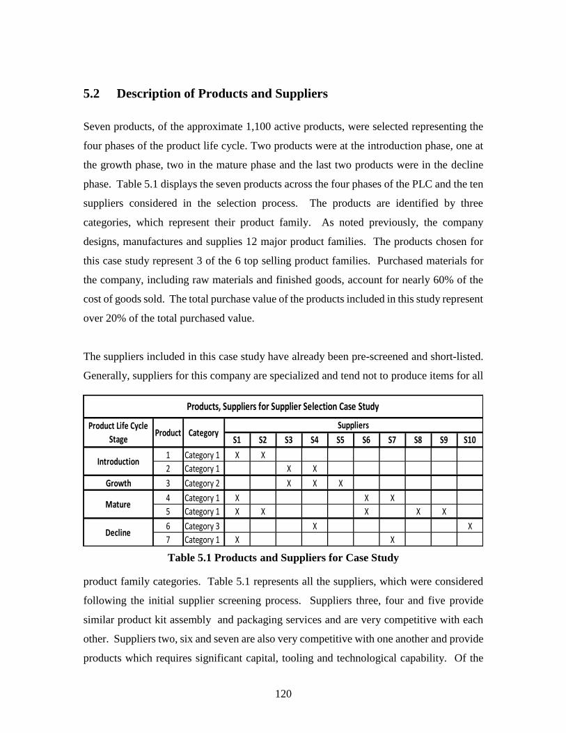
120
5.2 Description of Products and Suppliers
Seven products, of the approximate 1,100 active products, were selected representing the
four phases of the product life cycle. Two products were at the introduction phase, one at
the growth phase, two in the mature phase and the last two products were in the decline
phase. Table 5.1 displays the seven products across the four phases of the PLC and the ten
suppliers considered in the selection process. The products are identified by three
categories, which represent their product family. As noted previously, the company
designs, manufactures and supplies 12 major product families. The products chosen for
this case study represent 3 of the 6 top selling product families. Purchased materials for
the company, including raw materials and finished goods, account for nearly 60% of the
cost of goods sold. The total purchase value of the products included in this study represent
over 20% of the total purchased value.
The suppliers included in this case study have already been pre-screened and short-listed.
Generally, suppliers for this company are specialized and tend not to produce items for all
product family categories. Table 5.1 represents all the suppliers, which were considered
following the initial supplier screening process. Suppliers three, four and five provide
similar product kit assembly and packaging services and are very competitive with each
other. Suppliers two, six and seven are also very competitive with one another and provide
products which requires significant capital, tooling and technological capability. Of the
S1 S2 S3 S4 S5 S6 S7 S8 S9 S10
1 Category 1 X X
2 Category 1 X X
Growth 3 Category 2 X X X
4 Category 1 X X X
5 Category 1 X X X X X
6 Category 3 X X
7 Category 1 X X
Products, Suppliers for Supplier Selection Case Study
Suppliers
Introduction
Mature
Product Life Cycle
StageCategory
Decline
Product
Table 5.1 Products and Suppliers for Case Study

121
ten suppliers, only suppliers three and four are capable of producing items from two or
more categories included in this case study. Supplier four is the only vendor able to provide
products from all three categories. Several new suppliers, including 1, 8 and 10, were
included in the selection process.
Vendors for the introduction products are considered and added to the short list of potential
suppliers based on past history and performance. New supply sources are included on this
short list if they are able to provide new technology that is not available within the existing
supply chain capabilities. Additional revenue is the motivation for existing suppliers to
compete for introductory products, not to mention the competitive advantage gained by
providing products in the introduction phase of the PLC.
Yearly demand in number of units for the seven products is shown in Table 5.2. Demand
ranges from 15,000 to 340 million units, with the decline products having the lowest
quantities. DM3 provided the yearly demand information. Her job responsibilities
necessitate utilizing yearly demand forecasts in order to insure suppliers have the necessary
capacity required to meet the forecasted demand levels. As noted previously, the items
from the growth and mature products require significant capital, tooling and technological
capability and represent the highest yearly demands.
Table 5.2 Yearly Unit Product Demand

122
5.3 Key Supplier Selection Criteria
Suppliers were evaluated based on 10 criteria for the four phases of the product life cycle.
The Manager of Global Purchasing provided the 10 criteria and definitions used in the case
study. They are included in the company’s evaluation and selection processes. The criteria
are briefly described below:
▪ Product Safety- all products are tested for hazardous materials and heavy metals
via a U.S. national safety testing laboratory. Suppliers are required to provide the
testing lab with formulations details (confidentiality of suppliers’ intellectual
property is strictly maintained by the testing laboratory).
▪ Quality- suppliers must adhere to International Council of Toy Industries (ICTI)
Code of Conduct (http://www.toy-icti.org/). ICTI and its member associations
are committed to the promotion of toy safety standards, to the reduction or
elimination of barriers to trade and to the advancement of social responsibility in
the industry with programs to address environmental concerns, fair and lawful
employment practices and workplace safety. New and existing suppliers are
subject to extensive on-site quality audits conducted by the company’s quality
assurance personnel. These factory process quality audits include evaluation of
the adherence to quality control procedures and policies. Compliance with
standard safety procedures, such as access to machine guarding, fire
extinguishers, electrical panels, emergency exits, etc. is included in the quality
evaluation. In addition to the audit of these quality control processes, the ethical
treatment of employees is a key attribute included in the assessment process.
▪ Product performance- relates to the supplier’s ability to meet the company’s
product specifications including safety. This criterion also includes the proper
handling of raw materials, which are frequently provided by the company. These
raw materials may include proprietary formulations, which are not shared with the
supplier in order to protect the company’s intellectual property.
▪ Tooling development time- is evaluated based on the ability to meet product
shipment requirements. Slow tooling development time is considered a negative

123
attribute when selecting suppliers for introduction phase products. Suppliers with
in-house tooling development capability for dies have a competitive advantage.
▪ Pricing- includes the unit price and tooling cost, which is unitized based on
expected total purchase quantity.
▪ Advanced Technology- is evaluated based on the application with respect to
processes, product solutions and cost reductions throughout the product life cycle.
The ability of suppliers to quickly respond to problems using advanced
technology is critical.
▪ Delivery- is the actual supplier performance compared to the agreed upon
delivery dates.
▪ Lead-time- is assessed based on the supplier’s total expected time from order
placement to shipment.
▪ Service/Capacity Planning- is defined as the ability to deliver product according
to required delivery schedule. This criterion requires suppliers to provide a
detailed capacity plan based on supplier capacity, expected demand and delivery
requirements.
▪ Past Performance- is the supplier’s historical performance including delivery,
lead-time, problem solving, pricing performance, safety adherence, product
performance and quality. This represents an overall assessment of the supplier’s
performance.
Not all supplier selection criteria are utilized in all phases of the PLC. For example, past
performance is not included in the introduction phase of the product life cycle, because
there is no past performance history for a newly introduced product. Advanced
technology is excluded from the growth, mature and decline phases of the product life
cycle, but is a critical criterion for new products in the introduction phase. Past
performance is also excluded from the growth phase since the history would be limited to
the introduction phase. These decisions were made in consultation with the company
personnel.

124
Suppliers’ performance on the selection criterion was rated on a scale of 1 to 10, with 10
being the highest and 1 being the lowest. Table 5.3 gives the supplier ratings, as well as
the maximum business levels for each of the vendors. This information was provided by
DM3, whose job responsibilities include having detailed knowledge and monitoring of
supplier performance. The maximum business level is determined as a percentage of
the supplier’s overall sales revenue in U.S. dollars. The business levels for each supplier
are researched and utilized in the overall sourcing decisions. This is a conscious effort to
make sure that suppliers do not become too reliant on the company for their revenues and
related profits. Landry (1998) termed this limiting of overall business as a power
balance, which needs to be maintained in the customer-supplier relationship. Landry’s
study recommended the power balance to be between 20% and 40% of the business
revenue of a specific supplier. While there was no reference to Landry by the company
in setting the maximum business levels, the intention of limiting business supports
Landry’s goals of maintaining a healthy customer-supplier relationship. Note that several
supplier’s maximum business levels are below the 20% lower limit referenced by Landry.
The decision to use a level lower than 20% was focused on new suppliers (e.g. supplier
S8). Since there was limited history with these suppliers, the company decided to further
limit overall purchasing levels in an effort to reduce risk with these potential new supply
sources.
S1 S2 S3 S4 S5 S6 S7 S8 S9 S10
Product Safety 10.0 10.0 8.0 9.0 9.0 10.0 10.0 10.0 10.0 10.0
Quality 9.5 9.5 8.0 9.0 9.0 9.5 95.0 7.0 9.5 9.5
Product Performance 9.5 9.5 9.0 9.0 9.0 9.5 9.5 7.0 9.5 9.5
Tooling Development Time 6.0 9.0 8.0 8.0 8.0 7.0 9.0 5.0 9.0 9.0
Pricing
Advanced Technology 6.0 8.0 8.0 8.0 6.0 6.0 7.0 2.0 7.0 8.0
Delivery 9.5 9.0 9.5 9.5 9.5 9.0 9.0 6.0 9.0 8.0
Lead-Time 8.0 9.0 9.0 9.0 9.0 9.0 9.0 6.0 9.0 8.0
Service/Capacity Planning 8.0 9.0 8.0 8.0 8.0 9.0 9.0 6.0 8.0 8.0
Past Performance 8.0 9.0 8.0 8.0 8.0 9.0 9.0 6.0 9.0 8.0
Maximum Amount of Business* 20 40 40 30 20 40 40 10 30 20
* percentage of total sales $'s
Supplier Ratings vs. Key Criteria
SuppliersRating Criteria
Pricing varies by Product
Table 5.3 Supplier Performance Ratings and Maximum Business Levels
125
The next section explains the key decision maker ranking methods used and the results
for the selection criteria across the product life cycle.
5.4 Ranking the Product Life Cycle Phases
The DMs for this case study will be identified by the following convention:
▪ Chief Operating Officer (COO) is designated DM1;
▪ Vice President of Procurement is designated DM2;
▪ Manager of Global Purchasing is designated DM3.
A number of multiple criteria ranking methods were employed in this case study to rank
the product life cycle phases and the supplier selection criteria. A brief explanation of each
of the method follows:
Rating method: A rating scale of 1 to 10 is employed. The rating for each of the criterion
is then normalized to get the criteria weights. The criterion weight is obtained by dividing
its rating by the sum of all criteria ratings. This method poses the least cognitive burden on
the decision maker.
Borda count utilizing pairwise comparison: Each DM completes a pairwise comparison
of the criteria. A pairwise comparison matrix identifies preferences of criterion (e.g.
introduction vs. growth PLC phase). Preferences are recorded in the pairwise comparison
matrix as a 1 (preferred) or 0 (not preferred) and the rows are summed for each criterion.
Finally, the weight for each criterion is computed by dividing its row sum by the sum of
all row sums. This method poses a moderate level of cognitive burden.
Analytic Hierarchy Process (AHP): DM’s provide the strength of preference in addition
to the pairwise comparison of criteria utilized in the Borda count method. A numerical
score representing a weight is then calculated for each criterion as discussed in Chapter 2.
AHP poses the highest cognitive burden on the decision maker.
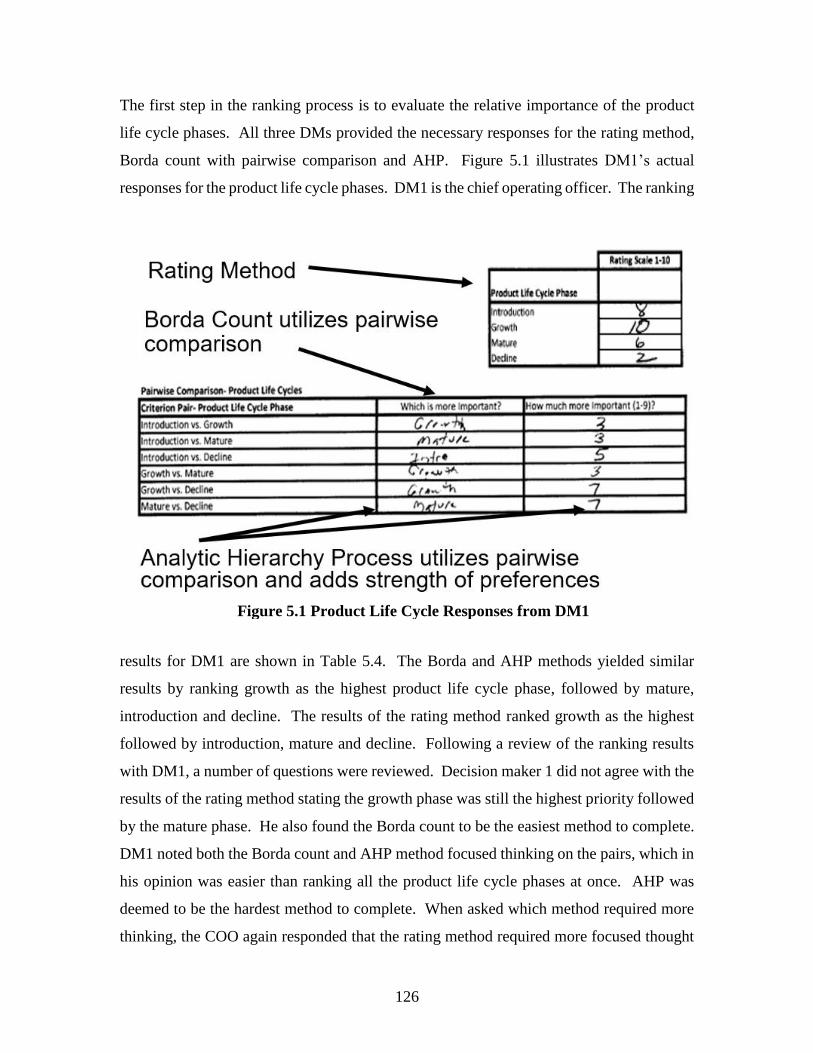
126
The first step in the ranking process is to evaluate the relative importance of the product
life cycle phases. All three DMs provided the necessary responses for the rating method,
Borda count with pairwise comparison and AHP. Figure 5.1 illustrates DM1’s actual
responses for the product life cycle phases. DM1 is the chief operating officer. The ranking
results for DM1 are shown in Table 5.4. The Borda and AHP methods yielded similar
results by ranking growth as the highest product life cycle phase, followed by mature,
introduction and decline. The results of the rating method ranked growth as the highest
followed by introduction, mature and decline. Following a review of the ranking results
with DM1, a number of questions were reviewed. Decision maker 1 did not agree with the
results of the rating method stating the growth phase was still the highest priority followed
by the mature phase. He also found the Borda count to be the easiest method to complete.
DM1 noted both the Borda count and AHP method focused thinking on the pairs, which in
his opinion was easier than ranking all the product life cycle phases at once. AHP was
deemed to be the hardest method to complete. When asked which method required more
thinking, the COO again responded that the rating method required more focused thought
Figure 5.1 Product Life Cycle Responses from DM1

127
since other factors relating to product performance had to be simultaneously considered,
whereas the Borda and AHP provided a comparison of one PLC phase versus another via
the paired comparisons. Overall DM1 noted that the Borda and AHP rankings matched his
thinking most closely. Although DM1 ranked the growth phase highest followed by the
mature phase, he commented “there is no growth phase without a successful introduction
phase.”
Decision Maker 2’s ranking results are presented in Table 5.5. The results for the Borda
and AHP methods match but differ from the rating method with respect to the rankings of
the introduction and growth phases. DM2 chose introduction as the most important PLC
phase in the rating method. He noted introduction was the most important phase because
getting a product launched on time and to the customer is critical. Without a successful
introduction phase, there would be no growth phase for the new product. Getting it right
from the start is critical which includes product design, manufacturing and shipping. He
also noted that the focus of the introduction and growth phases was “chasing revenue
versus margin”. DM2 continued “typically a mature product has done well on the shelf,”
generating a solid sales volume. Given this good sales volume, the mature phase focus
was directed at generating revenue with the focus changing to “chasing margin versus
revenue.”
Product Life Cycle (PLC) Phase
Rating
Method
Borda
Method AHP
Introduction 2 3 3
Growth 1 1 1
Mature 3 2 2
Decline 4 4 4
Comparison of DM1 (Chief Operating Officer)
Rankings for Product Life Cycle Phase
Table 5.4 Ranking of PLC Phases by Different Methods for DM1

128
DM2 found the rating method to be the easiest, since it allowed the PLC phases to be put
in a linear order which reduced the complexity of the rating process. AHP was deemed to
be the hardest ranking method and required the greatest cognitive effort, given there were
more things to consider such as the pair-wise comparisons and the strength of preference.
Overall, the rating method matched DM2’s thinking with respect to the product life cycle
phase rankings.
DM3’s ranking results are shown in Table 5.6. The ranking results are different for each
of the ranking methods. DM3 stated the growth phase was most important to make sure a
product is thriving as this starts to gain market share and add to the revenue stream of the
company. Increasing volume for a growth phase product also allows procurement
professionals to improve item pricing. This possible benefit of improved pricing can be
contrasted with the introduction phase. In the introduction phase the objective is to “get
the product on the shelf at the right profit margin as compared to the best possible profit
margin.” Like DM2, she noted in the introduction phase you are “chasing revenue not
margin.”
DM3 found the rating method to be the easiest method, while AHP was harder to complete
given the pair-wise comparisons and the evaluation of the strength of preference. The
rating methods results were most consistent with DM3’s preferences. She felt the growth
phase could be very difficult to manage given demand spikes of up to 25%, hence the
Product Life Cycle (PLC) Phase
Rating
Method
Borda
Method AHP
Introduction 1 2 2
Growth 2 1 1
Mature 3 3 3
Decline 4 4 4
Comparison of DM2 (VP Procurement) Rankings for
Product Life Cycle Phase
Table 5.5 Ranking of PLC Phases by Different Methods for DM2
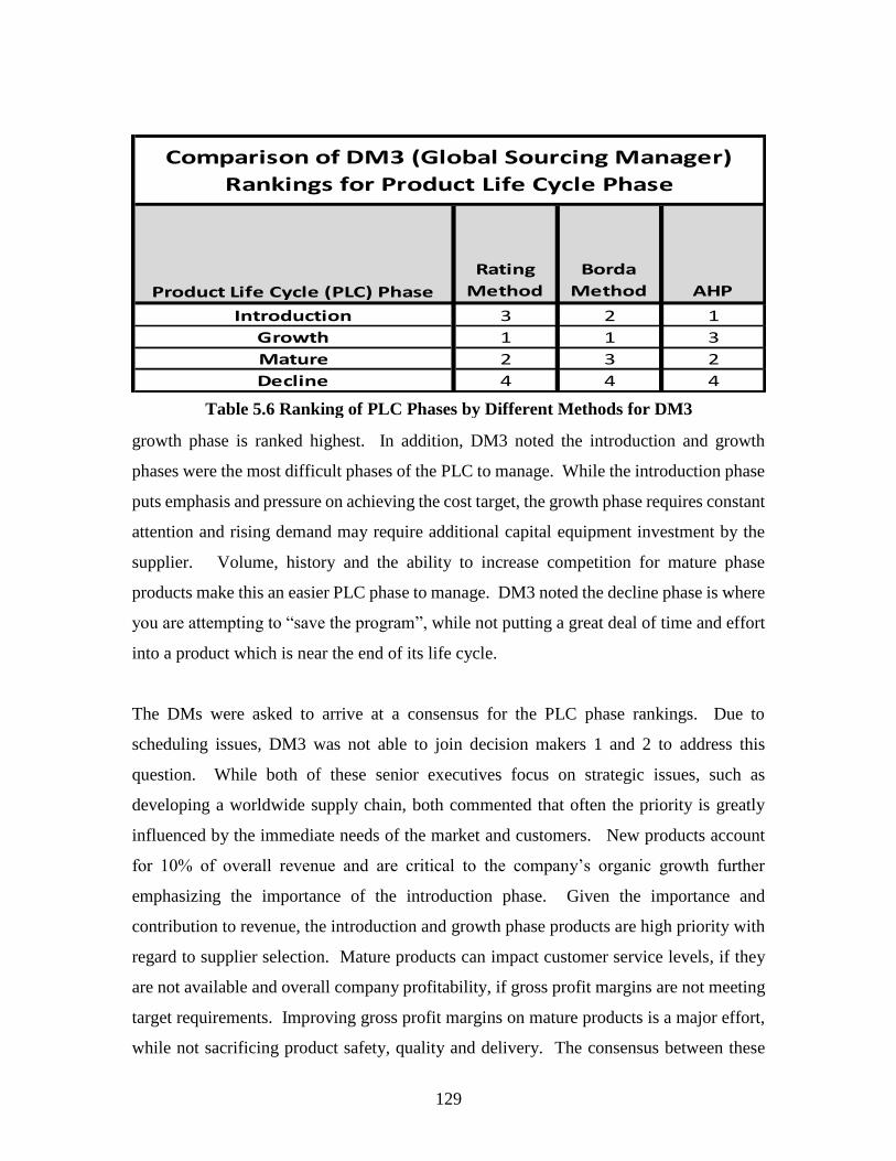
129
growth phase is ranked highest. In addition, DM3 noted the introduction and growth
phases were the most difficult phases of the PLC to manage. While the introduction phase
puts emphasis and pressure on achieving the cost target, the growth phase requires constant
attention and rising demand may require additional capital equipment investment by the
supplier. Volume, history and the ability to increase competition for mature phase
products make this an easier PLC phase to manage. DM3 noted the decline phase is where
you are attempting to “save the program”, while not putting a great deal of time and effort
into a product which is near the end of its life cycle.
The DMs were asked to arrive at a consensus for the PLC phase rankings. Due to
scheduling issues, DM3 was not able to join decision makers 1 and 2 to address this
question. While both of these senior executives focus on strategic issues, such as
developing a worldwide supply chain, both commented that often the priority is greatly
influenced by the immediate needs of the market and customers. New products account
for 10% of overall revenue and are critical to the company’s organic growth further
emphasizing the importance of the introduction phase. Given the importance and
contribution to revenue, the introduction and growth phase products are high priority with
regard to supplier selection. Mature products can impact customer service levels, if they
are not available and overall company profitability, if gross profit margins are not meeting
target requirements. Improving gross profit margins on mature products is a major effort,
while not sacrificing product safety, quality and delivery. The consensus between these
Product Life Cycle (PLC) Phase
Rating
Method
Borda
Method AHP
Introduction 3 2 1
Growth 1 1 3
Mature 2 3 2
Decline 4 4 4
Comparison of DM3 (Global Sourcing Manager)
Rankings for Product Life Cycle Phase
Table 5.6 Ranking of PLC Phases by Different Methods for DM3
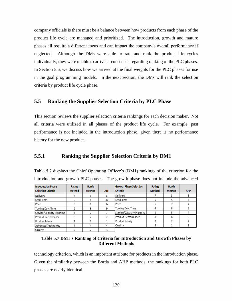
130
company officials is there must be a balance between how products from each phase of the
product life cycle are managed and prioritized. The introduction, growth and mature
phases all require a different focus and can impact the company’s overall performance if
neglected. Although the DMs were able to rate and rank the product life cycles
individually, they were unable to arrive at consensus regarding ranking of the PLC phases.
In Section 5.6, we discuss how we arrived at the final weights for the PLC phases for use
in the goal programming models. In the next section, the DMs will rank the selection
criteria by product life cycle phase.
5.5 Ranking the Supplier Selection Criteria by PLC Phase
This section reviews the supplier selection criteria rankings for each decision maker. Not
all criteria were utilized in all phases of the product life cycle. For example, past
performance is not included in the introduction phase, given there is no performance
history for the new product.
5.5.1 Ranking the Supplier Selection Criteria by DM1
Table 5.7 displays the Chief Operating Officer’s (DM1) rankings of the criterion for the
introduction and growth PLC phases. The growth phase does not include the advanced
Table 5.7 DM1’s Ranking of Criteria for Introduction and Growth Phases by
Different Methods
technology criterion, which is an important attribute for products in the introduction phase.
Given the similarity between the Borda and AHP methods, the rankings for both PLC
phases are nearly identical.

131
For the introduction phase, the rating method results substantially differ on product
performance, service and capacity planning, when compared to the Borda and AHP results.
Safety is a top priority for DM1 for all product life cycle phases and the ranking results
reflect this preference. Other top priorities in the introduction phase are quality and product
performance. Without high quality and product performance, sales would be negatively
impacted. Advanced technology would be an important criterion for supplier evaluation
in the introduction phase. Tooling development earned the lowest ranking in introduction
and DM1 noted that tooling is somewhat fixed and known, along with lead-time and
therefore leads to a lower ranking.
Product quality and safety are top ranked criteria in the growth phase for all methods. DM1
ranked price and product performance in the bottom 3 criteria for all approaches. He noted
that the Borda and AHP ranking results were most consistent with his criteria ranking. As
experienced in the PLC phase rating process, DM1 preferred the Borda and AHP methods
for ranking criteria.
Table 5.8 displays the ranking results by the different methods for DM1 for the mature and
decline phases. The results of the Borda and AHP methods for the mature and decline
phases rank safety quality and price in the top 3. These rankings contrast the introduction
and growth phase, which ranked price and quality in the bottom half or bottom 3 criteria.
The COO noted that price was very important for the mature and decline phases given the
Table 5.8 DM1’s Ranking of Criteria for Mature and Decline Phases by Different
Methods

132
impact on the company’s gross profit margin. He noted that the focus on price for these
final PLC phases was essential. Demand for mature product should be relatively stable,
which simplifies a price negotiation with suppliers. DM1 agreed with the ranking results
for the top and bottom three criteria for the Borda and AHP ranking methods and they gave
the best overall match to his preferences on the criteria.
5.5.2 Ranking the Supplier Selection Criteria by DM2
Table 5.9 presents the VP of Procurement’s (DM2) rankings for the introduction and
growth phases of the PLC. DM2 noted the importance of getting the product on the shelf
and performing to required specifications. Given these requirements, good quality and
delivery performance should be given high priority with respect to supplier selection. In
both the introduction and growth phases the emphasis is on generating revenue versus gross
profit margin. DM2 preferred the Borda and AHP rankings, and they were most consistent
with the importance he placed on quality, safety, delivery and product performance.
As products migrate from introduction and growth to the mature product life cycle phase,
the emphasis on improving the gross profit margin significantly increases. Once again,
DM2 agreed with the Borda and AHP rankings for the mature and decline product life
cycle phases shown in Table 5.10. Given the emphasis on gross profit margin, DM2 ranked
price in the top 3 selection criteria, following safety and quality. A mature product for this
Table 5.9 DM2’s Ranking of Criteria for Introduction and Growth Phases by
Different Methods

133
company has typically done well in terms of unit sales and should be part of a repeatable
buy with a number of alternative sources. Therefore, supplier selection practices should
include strategic sourcing with an emphasis on creating price competition within the supply
base in order to improve the overall gross margin of the purchased product. Unlike the
introduction and growth phases, the focus is on revenue; hence, the mature phase changes
the focus to increasing gross margin. DM2 has the same top 3 ranking for quality, safety
and price for decline products. Ideally DM2 would prefer for any of his procurement team
not to be directly involved or utilized in activity relating to a decline phase product, since
they are being phased out or being replaced by a product in the introduction phase.
5.5.3 Ranking the Supplier Selection Criteria by DM3
Table 5.11 displays the Global Sourcing Manager’s (DM3) ranking results for the
introduction and growth phases. DM3 ranked safety, quality and delivery as the top criteria
in the introduction PLC phase. She noted that you are not able to successfully launch a
new product without solid performance in these key supplier attributes. In addition, she
also supported the VP of Procurement’s assertion that the focus of the introduction phase
is achieving the revenue targets for the new product as opposed to gross profit margin
contribution.
Table 5.10 DM2’s Ranking of Criteria for Mature and Decline Phases by Different
Methods

134
Table 5.11 DM3’s Ranking of Criteria for Introduction and Growth Phases by
Different Methods
DM3 noted that the growth PLC phase was very similar to the introduction phase with its
emphasis on quality and safety. In addition to safety and quality, lead-time becomes very
important as sales volume increases or demand spikes in the growth phase. DM3
commented that the introduction and growth phases are the most difficult to manage.
Delivery schedules must be met, cost targets must be achieved and unexpected demands
can create havoc for the entire supply chain.
Table 5.12 presents the criteria rankings for DM3 for the mature and decline phases. As
the global purchasing manager, she commented that the mature phase allows you to “spice
it up” and focus on increasing price competition among the suppliers. While safety and
quality are the top 2 criteria, price is ranked third in both the Borda the AHP results. The
Table 5.12 DM3’s Ranking of Criteria for Mature and Decline Phases by Different
Methods

135
price competition between qualified suppliers, with excellent safety and quality
performance, provides the opportunity to improve the company’s gross profit margin.
While issues with the decline phase product has to be addressed, ideally the effort should
be minimized given the product has reached the end of its life cycle. The goal to minimize
the efforts on the decline products parallels DM2’s objective. DM3 preferred the Borda
and AHP results versus the rating method for all four phases of the product life cycle.
5.6 Final Ranking and Weights for the MCDM Supplier Selection
Models
The ranking results from all three decision makers will be incorporated into the supplier
selection MCDM models in Chapter 6. Since all three executives preferred the results of
the Borda and AHP methods, the results of the AHP ranking method will be used to
determine the weights utilized by the supplier selection models. The next section will
review these ranking results and illustrate the corresponding weights obtained from the
rankings.
5.6.1 Ranking and Weights of PLC Phases
It is interesting to review the ranking method that each of the decision makers preferred.
DM1 favored Borda and AHP methods since these methods focused thinking in pairs as
compared to ranking all the PLC phases or supplier selection attributes at once. Decision
makers 2 and 3 preferred the rating method based on cognitive burden. The rating method
also most closely matched their thinking regarding the PLC phases. It is interesting to
observe that all 3 DMs preferred the ranking results of the Borda and AHP methods for the
PLC supplier selection attributes. The average AHP weights for the product life cycle
phases and supplier selection criteria will be incorporated into the non-preemptive GP
model in Chapter 6. Table 5.13 displays the AHP weights for each decision maker for the
product life cycle phases.

136
5.6.2 Final Criteria Weights by PLC Phase
Table 5.14 displays the average AHP weights for the supplier selection criteria by PLC
phase. The supplier selection results from decision makers 1 and 2 are nearly identical for
the top 3 criteria of growth, mature and decline phases. They only differ on the top 3
ranking results for the introduction phase criteria. In the introduction phase, DMs 1 and 2
agree on 2 of the 3 top criteria ranking product safety first and quality second. They only
differ on product performance and delivery. In spite of some differences in rankings
between the decision makers, it is clear all ranked quality and safety as top supplier
selection criteria for all phases of the PLC. The differences in the ranking results may be
attributed to the decision makers’ specific job responsibilities. DMs 1 and 2 may take a
more strategic view of the supplier selection criteria whereas DM3 may be focused on
tactical day to day requirements of the supplier selection process.
5.6.3 Overall Weights for the Goal Programming Models
The overall weights for the goal programming models, used in Chapter 6, are calculated by
multiplying the product life cycle phase weights by the respective weights of the supplier
selection criteria. Table 5.15 presents the final weights for the supplier selection models
by PLC phase and supplier selection criteria. The PLC supplier selection criteria AHP
weights were averaged for all the DMs prior to being multiplied by the PLC phase average
weights. The overall weights are listed in descending order representing the rank order of
goal priority for the preemptive GP. In the next section, the minimum and maximum
DM1 DM2 DM3
Average PLC
Weight
Introduction 16.2% 29.3% 47.7% 31.1%
Growth 49.7% 53.1% 14.4% 39.1%
Mature 29.4% 13.7% 33.4% 25.5%
Decline 4.7% 3.9% 4.5% 4.4%
Product Life
Cycle Phase
AHP Weights
Table 5.13 Average AHP weights by PLC Phase

137
number of suppliers by product life cycle phase will be discussed.
Table 5.15 Overall AHP Weights for Goal Programming
Table 5.14 Average AHP Weights by PLC Phase and Supplier Selection Criteria

138
5.7 Minimum and Maximum Number of Suppliers by PLC Phase
The decision makers were also asked to record the minimum and maximum number of
suppliers which could be utilized by product life cycle phase. This information would be
utilized to create constraints on the number of suppliers in each of the goal programs. Table
5.16 displays the min-max number of suppliers by PLC phase obtained from the decision
makers. All three DM’s recommended one supplier as the minimum number of suppliers
for the introduction phase (products 1 and 2), while the maximum number ranged from one
to three. Based on discussion with these key executives and their emphasis on “getting the
product on the shelf” both the minimum and maximum number of suppliers was set at one.
This would reduce complexity in dealing with startup issues and also was a practical
decision since there were only two potential short-listed suppliers for each of the
introduction products.
For the growth phase (product 3), the minimum number of suppliers was set to one and
the maximum number to two. Only three suppliers made the short list of possible suppliers.
The growth phase had the highest overall weight in the PLC ranking and all DM’s noted
the importance of this critical PLC phase. Allowing up to two suppliers would encourage
competition while not overly complicating the supply chain with too many suppliers.
Product Life Cycle Phase
Minimum
Number of
Suppliers
Maximum
Number of
Suppliers
Introduction 1 1
Growth 1 2
Mature 2 3
Decline 1 2
Minimum and Maximum Number of
Supplier by Product Life Cycle Phase
Table 5.16 Number of Suppliers by PLC Phase
139
For the mature phase (products 4 and 5), the number of short-listed suppliers for the two
products ranged from three to five. The minimum number of suppliers was set at two and
the maximum at three. This would still support competition among the suppliers by
guaranteeing that at least two suppliers would always be selected. This would allow the
DMs to “spice up” the competition with the objective of improving the overall gross margin
of the products. The executives were all consistently emphasizing the change from
generating revenue in the introduction and growth phases to generating improved margins
in the mature phase.
For the decline phase (products 6 and 7), the minimum and maximum number of suppliers
was set at one and two respectively. There were only two potential suppliers for both of
the decline products. Each of the decision makers commented that minimum procurement
effort should be applied to decline phase products. DM2 commented that as a product
transitions to the decline phase, there are fewer potential suppliers and decreased product
volumes. By minimizing the number of active decline phase suppliers, “it is easier to
manage scrap charges and the effects on a supplier’s health.”
The next chapter will describe the development and results of the goal programming
models for supplier selection and order allocation.

140
6. Case Study: Global Supplier Selection Problem across
Product Life Cycle – Supplier Selection and Order
Allocation Chapter 6 is focused on utilizing the supplier selection criteria weights and rankings,
detailed in Chapter 5. Goal programming methods will be employed in order to determine
the final supplier selections and order allocations for the case study. These goal
programming methods include:
▪ Preemptive;
▪ Non-preemptive;
▪ Tchebycheff’s min-max;
▪ Fuzzy.
Sections 4.3.3 to 4.3.6 respectively review the major characteristics of each of the GP
models. The next section will compare model statistics between the Chapter 4 illustrative
example and the case study for the preemptive GP model. This comparison will include
the number of variables and constraints, the time to solve and number of iterations.
Correlations among these model characteristics for the preemptive case study GP model
will also be analyzed.
6.1 Preemptive GP Model for the Case Study
Table 6.1 provides information
regarding major goal programming
attributes for the case study. The
case study is substantially larger
than the illustrative example,
presented in Chapter 4, with nearly
quadruple the number of real
variable and double the number of
real constraints. The number of real
variables in the case study are equal
to 62, integer variables are equal to
Case StudyNumber of Integer Variables 38
Number of Real Variables 62
Number of Deviational Variables 124
Total Number of Variables 224
Number of Goal Constraints 62
Number of Real Constraints 238
Total Number of Constraints 300
Time to Solve (seconds) 0.11
Table 6.1 Preemptive GP Model Characteristics
for the Case Study

141
38, deviational variables are equal to 124. The case study has 62 goal constraints and 238
real constraints. The model was solved using LINGO Version 17.0.74, which is an
optimization modeling software for linear, nonlinear, and integer programming. The
model took less than one second to solve running on a Dell Inspiron Model 7773 Laptop
Computer, using an Intel Core i7-8550U CPU at 1.80 GHz, and Windows 10 operating
system. Although the model took less than one second to solve, the number of integer
variable is highly correlated to time to solve. Ravindran, Phillips and Solberg (1987) note
the relationship between number of integer variable and time to solve and provide
recommendations for utilizing integer variables.
6.1.1 Preemptive GP Priorities
In preemptive goal programming, the DM identifies the order in which goal constraints
will be achieved after setting the target levels. The target levels were set at 95% of the
ideal values for maximization and 105% of ideal values for minimization objectives. This
relaxing of target values provides some flexibility with respect to attaining the conflicting
objectives.
In the case study, the DM’s ranked the goals from highest to lowest priority. This ranking
was generated by averaging the AHP weights for the PLC phase and the PLC phase
selection criteria, which was detailed in Sections 5.6.2 and 5.6.3. The average weights,
which were generated by multiplying the average PLC phase weight by the PLC supplier
selection criteria, were then enumerated in descending order. This order provided the goal
achievement priority order for the preemptive GP model. Table 6.2 displays the selection
criteria in priority order by product life cycle phase and criterion. The decision makers
ranked the growth phase highest followed by the introduction, mature and decline phases.
The quality and safety criteria were ranked highest and represent the top 5 criteria to be
achieved. Delivery performance was another highly ranked criterion for growth and
introduction phases. The decline phase was ranked the lowest and represents the bottom
third of the selection criteria priorities. It should be noted that price is the only criterion
that is minimized. All other selection criteria are maximized.

142
Selection
Criteria Priority
Order
Product Life
Cycle Stage Selection Criteria
1 Growth Maximize Quality Performance
2 Growth Maximize Product Safety Performance
3 Introduction Maximize Product Safety Performance
4 Mature Maximize Product Safety Performance
5 Mature Maximize Quality Performance
6 Growth Maximize Delivery Performance
7 Introduction Maximize Quality Performance
8 Introduction Maximize Delivery Performance
9 Introduction Maximize Product Performance
10 Growth Maximize Lead-Time Performance
11 Growth Maximize Service/Capacity Planning Performance
12 Growth Maximize Product Performance
13 Growth Minimize Price
14 Mature Maximize Product Performance
15 Mature Minimize Price
16 Mature Maximize Maximize Past Performance
17 Introduction Minimize Price
18 Mature Maximize Delivery Performance
19 Introduction Maximize Advanced Technology Rating
20 Introduction Maximize Lead-Time Performance
21 Introduction Maximize Service/Capacity Planning Performance
22 Growth Maximize Tooling Development Time Performance
23 Mature Maximize Service/Capacity Planning Performance
24 Introduction Maximize Tooling Development Time Performance
25 Mature Maximize Lead-Time Performance
26 Decline Maximize Product Safety Performance
27 Decline Maximize Quality Performance
28 Mature Maximize Tooling Development Time Performance
29 Decline Minimize Price
30 Decline Maximize Maximize Past Performance
31 Decline Maximize Service/Capacity Planning Performance
32 Decline Maximize Product Performance
33 Decline Maximize Delivery Performance
34 Decline Maximize Lead-Time Performance
35 Decline Maximize Tooling Development Time Performance
Table 6.2 Preemptive GP Supplier Selection Priorities

143
6.1.2 Preemptive GP Solution
The goal constraints are solved sequentially according to the priority order, shown in Table
6.2. This requires that the optimal solution for priority 1, which is the maximization of the
growth phase quality performance be determined first. The achieved value for priority 1
is then inserted as a real constraint in the priority 2 GP model. This ensures the
achievement of the priority 1 goal is maintained during the solution of priority 2, which is
the maximization of the growth phase safety performance. In other words, while
optimizing the priority 2 goal, only the alternative optimal solutions of priority 1 goal are
considered. This process continues as long as alternative optima exist at an iteration. This
insures the achievement of the higher priorities are maintained before the lower priority
goals are even considered. Hence, when the GP model reaches a unique optimal solution
from some priority, the algorithm stops since no improvements to lower priority goals are
possible. This ordering of priorities reduces the cognitive burden on the DM. Additionally,
objectives/goals do not have to be scaled. The next sections will review the supplier
selections and order allocations for each product and its corresponding product life cycle
phase.
6.1.3 Introduction Phase Results (Product 1)
Table 6.3 displays the
procurement plan for introduction
phase (product 1). Supplier 1 was
chosen to supply the entire yearly
demand. A constraint limiting the
maximum number of suppliers for
the introduction phase to one does
not allow splitting the demand
between the two suppliers. Table 6.4 presents the preemptive goal achievements for the
supplier selection criteria with respect to the target values. The highest priorities, which
include safety, quality, delivery and product performance, achieve and surpass the target
values by 5.3%. Supplier 1’s performance is equal to or better than supplier 2 for all these
S1 S2
10,000,000 0
1 Maximum number of suppliers set to one supplier
Optimal Order Allocations to SuppliersSuppliers
Order Allocations1
Table 6.3 Preemptive GP Procurement Plan for
Introduction Phase Product 1

144
top 4 selection criteria. Price misses the target by 5.8%, since supplier 2’s price is
approximately 10% less than supplier 1. This is an example of higher goal constraints
being achieved at the detriment of lower priority goals. Likewise, all the remaining goals
including advanced technology, lead-time, service/capacity planning and tooling
development time miss the target values. The tooling development time records the largest
target miss at 29.8%.
6.1.4 Introduction Phase Results (Product 2)
Table 6.5 displays the
procurement plan for the
introduction phase (product 2).
Supplier 3 was chosen to supply
the entire yearly demand. Table
6.6 presents the preemptive goal
achievements for the supplier
selection criteria with respect to
the target values. Unlike product 1, the two highest priorities for maximizing safety and
quality performance miss the target achievement by 6.4%. This result may seem
counterintuitive given the high goal priority for these criteria. Detailed testing of the model
revealed the achievement of goal priorities 1 and 2 for growth phase product 3, have a
Goal
Priority
Order Selection Criteria
Target Values
(95% or 105%
of Ideals)
Goal
Achievements Target Achievement
3 Maximize Product Safety Performance 95,000,000 100,000,000 Exceeded by 5.3%
7 Maximize Quality Performance 90,250,000 95,000,000 Exceeded by 5.3%
8 Maximize Delivery Performance 90,250,000 95,000,000 Exceeded by 5.3%
9 Maximize Product Performance 90,250,000 95,000,000 Exceeded by 5.3%
17 Minimize Price 472,500 500,000 Missed by 5.8%
19 Maximize Advanced Technology Rating 76,000,000 60,000,000 Missed by 21.1%
20 Maximize Lead-Time Performance 85,500,000 80,000,000 Missed by 6.4%
21 Maximize Service/Capacity Planning Performance 85,500,000 80,000,000 Missed by 6.4%
24 Maximize Tooling Development Time Performance 85,500,000 60,000,000 Missed by 29.8%
S3 S4
50,000 0
1 Maximum number of suppliers set to one supplier
Optimal Order Allocations to SuppliersSuppliers
Order Allocations1
Table 6.4 Preemptive GP Achievements for Introduction Phase Product 1 with
respect to Target Values
Table 6.5 Preemptive GP Procurement Plan for
Introduction Phase Product 2

145
direct impact on the supplier selection and order allocation of product 2. Supplier 4 clearly
had the best performance rating with respect to safety and quality, yet supplier 3 was
selected. Supplier 4 was chosen to supply 1.6 million units of product 3, which consumes
the entire capacity of supplier 4 with respect to business volume levels. This business
volume constraint combined with the best performance with respect to quality and safety
required the selection of supplier 4 for product 3. Achieving these higher priority goals
was again done at the detriment of the lower priority goals. This real example clearly
demonstrates the principles of preemptive goal programming. Ironically, all remaining
goals exceeded the target values by 4.8 to 5.3%. These goal achievements are possible
because of supplier 3’s better performance for delivery to tooling development time.
Table 6.6 Preemptive GP Achievements for Introduction Phase Product 2 with
respect to Target Values
6.1.5 Growth Phase Results (Product 3)
Table 6.7 displays the procurement plan for the growth phase (product 3). Suppliers 3 and
4 were chosen to supply the yearly demand. A constraint limiting the maximum number
of suppliers for the growth phase to two allows splitting the demand between the two
suppliers. Table 6.8 presents the preemptive goal achievements for the supplier selection
Goal
Priority
Order Selection Criteria
Target Values
(95% or 105%
of Ideals)
Goal
Achievements Target Achievement
3 Maximize Product Safety Performance 427,500 400,000 Missed by 6.4%
7 Maximize Quality Performance 427,500 400,000 Missed by 6.4%
8 Maximize Delivery Performance 451,250 475,000 Exceeded by 5.3%
9 Maximize Product Performance 427,500 450,000 Exceeded by 5.3%
17 Minimize Price 91,350 87,000 Exceeded by 4.8%
19 Maximize Advanced Technology Rating 380,000 400,000 Exceeded by 5.3%
20 Maximize Lead-Time Performance 427,500 450,000 Exceeded by 5.3%
21 Maximize Service/Capacity Planning Performance 380,000 400,000 Exceeded by 5.3%
24 Maximize Tooling Development Time Performance 380,000 400,000 Exceeded by 5.3%

146
criteria with respect to the target values. Product 3 has the top 2 goal priorities in the
preemptive GP model maximizing quality and safety performance respectively. The
achievement of these goal priorities impacted the supplier selection process and order
allocations to the detriment of introduction phase (product 2). Even though product 3 has
the top goal priorities, both the quality and safety goal achievements did not achieve the
target values with both missing by 0.2%. Model testing revealed that while suppliers 4 and
5 had the best performance for both quality and safety, supplier 5 was not selected due the
business level constraint and the maximum limit of two suppliers for the growth phase
product. This business level constraint also resulted in the supplier 4 supplying the
maximum allowed volume of 1.6 million units. The remaining units would be supplied by
supplier 3. The supplier selection and order allocation for growth phase (product 3)
demonstrate the impact of both business constraints and goal achievements requirements.
The remaining goal constraints, except for price, exceed the target levels by 5.3%. Price
missed the target by 3%.
Goal
Priority
Order Selection Criteria
Target Values
(95% or 105%
of Ideals)
Goal
Achievements Target Achievement
1 Maximize Quality Performance 25,650,000 25,600,000 Missed by 0.2%
2 Maximize Product Safety Performance 25,650,000 25,600,000 Missed by 0.2%
6 Maximize Delivery Performance 27,075,000 28,500,000 Exceeded by 5.3%
10 Maximize Lead-Time Performance 25,650,000 27,000,000 Exceeded by 5.3%
11 Maximize Service/Capacity Planning Performance 22,800,000 24,000,000 Exceeded by 5.3%
12 Maximize Product Performance 25,650,000 27,000,000 Exceeded by 5.3%
13 Minimize Price 27,342,000 28,152,000 Missed by 3%
22 Maximize Tooling Development Time Performance 22,800,000 24,000,000 Exceeded by 5.3%
S3 S4 S5
1,400,000 1,600,000 0
Optimal Order Allocations to SuppliersSuppliers
Order Allocations1
1 Maximum number of suppliers set to two suppliersTable 6.7 Preemptive GP Procurement Plan for Growth Phase Product 3
Table 6.8 Preemptive GP Achievements for Growth Phase Product 3 with respect to
Target Values

147
6.1.6 Mature Phase Results (Product 4)
Table 6.9 displays the procurement plan for the mature phase (product 4). Suppliers 6 and
7 were chosen to supply the yearly demand. Table 6.10 presents the preemptive goal
achievements for the supplier selection criteria with respect to the target values. Several
real constraints also impacted the selection of the mature PLC phase products. These
constraints set the minimum number of required suppliers to two and the maximum number
of suppliers to three, which supports the DM’s objective of creating price competition in
order to improve the gross profit margin for mature phase products.
Product 4 exceeds or achieves the target values for 8 out of 9 goal priorities. The target
achievements range from 0.8% to 5.3%, with 6 out of 8 goal priorities achieving the latter.
Product 4, which has a high expected yearly demand of 340MM units, achieves the price
target supporting the decision maker’s goal of improving product gross profit margin. The
only goal achievement which missed the target value was tooling development time, which
missed the target value by 4.3%. This miss was due to selecting supplier 6, which has a
tooling score of 7, to supply nearly 60% of the total expected demand as compared to
supplier 7, which has a tooling score of 9. This is another example of higher priority goals
being achieved at the detriment of lower priority goals.
S1 S6 S7
0 200,600,000 139,400,000 1 Minimum number of suppliers set to two suppliers
Optimal Order Allocations to SuppliersSuppliers
Order Allocations1,2
2 Maximum number of suppliers set to three suppliersTable 6.9 Preemptive GP Procurement Plan for Mature Phase Product 4

148
Table 6.10 Preemptive GP Achievements for Mature Phase Product 4 with respect
to Target Values
6.1.7 Mature Phase Results (Product 5)
Table 6.11 displays the procurement plan for the mature phase (product 5). Suppliers 2
and 6 were chosen to supply the yearly demand of 110MM units. Table 6.12 presents the
goal achievements for the supplier selection criteria with respect to the target values.
Product 5 also requires a minimum of two suppliers and a maximum of three suppliers to
enhance competition among the suppliers, supporting improved gross profit margins for
mature phase products.
Product 5 exceeds the target values in 8 out of 9 goal priorities. The target achievements
range from 0.8% to 5.3%, with 6 out of 8 goal priorities achieving the latter. The price
goal priority exceeds the target by 4.8%, which like product 4, supports the DM’s goals of
improving gross profit margin for mature PLC phase products. Tooling development time
missed the target value by 13.5%. This miss was due to selecting supplier 6, which has a
tooling score of 7, to supply 80% of the total expected demand as compared to suppliers 2
and 9, which have tooling scores of 9.
Goal
Priority
Order Selection Criteria
Target Values
(95% or 105%
of Ideals)
Goal
Achievements Target Achievement
4 Maximize Product Safety Performance 3,230,000,000 3,400,000,000 Exceeded by 5.3%
5 Maximize Quality Performance 3,068,500,000 3,230,000,000 Exceeded by 5.3%
14 Maximize Product Performance 3,068,500,000 3,230,000,000 Exceeded by 5.3%
15 Minimize Price 14,994,000 14,994,000 Achieved Target
16 Maximize Past Performance 2,907,000,000 3,060,000,000 Exceeded by 5.3%
18 Maximize Delivery Performance 3,036,200,000 3,060,000,000 Exceeded by 0.8%
23 Maximize Service/Capacity Planning Performance 2,907,000,000 3,060,000,000 Exceeded by 5.3%
25 Maximize Lead-Time Performance 2,907,000,000 3,060,000,000 Exceeded by 5.3%
28 Maximize Tooling Development Time Performance 2,777,800,000 2,658,800,000 MIssed by 4.3%

149
6.1.8 Decline Phase Results (Product 6)
Table 6.13 displays the
procurement plan for decline
phase (product 6). Supplier 10
was chosen to supply the entire
yearly demand of 25,000 units.
Table 6.14 presents the
preemptive goal achievements for
the supplier selection criteria with
respect to the target values. The supplier selection for product 6 is impacted by the supplier
selection for growth phase (product 3). Product 3 had the top two goal priorities in the
preemptive model and supplier 4 was chosen to best achieve these goals. Selecting supplier
4 for product 3 consumed the entire capacity of supplier 4 based on business volume levels.
This previous supplier selection, which was determined via preceding goal constraints,
Goal
Priority
Order Selection Criteria
Target Values
(95% or 105%
of Ideals)
Goal
Achievements Target Achievement
4 Maximize Product Safety Performance 1,045,000,000 1,100,000,000 Exceeded by 5.3%
5 Maximize Quality Performance 992,750,000 1,045,000,000 Exceeded by 5.3%
14 Maximize Product Performance 992,750,000 1,045,000,000 Exceeded by 5.3%
15 Minimize Price 4,435,200 4,224,000 Exceeded by 4.8%
16 Maximize Past Performance 940,500,000 990,000,000 Exceeded by 5.3%
18 Maximize Delivery Performance 982,300,000 990,000,000 Exceeded by 0.8%
23 Maximize Service/Capacity Planning Performance 940,500,000 990,000,000 Exceeded by 5.3%
25 Maximize Lead-Time Performance 940,500,000 990,000,000 Exceeded by 5.3%
28 Maximize Tooling Development Time Performance 940,500,000 814,000,000 MIssed by 13.5%
S1 S2 S6 S8 S9
0 22,000,000 88,000,000 0 0
Optimal Order Allocations to SuppliersSuppliers
Order Allocations1,2
1 Minimum number of suppliers set to two suppliers2 Maximum number of suppliers set to three suppliers
S4 S10
0 25,000
Optimal Order Allocations to SuppliersSuppliers
Order Allocations1
1 Maximum number of suppliers set to two suppliers
Table 6.12 Preemptive GP Achievements for Mature Phase Product 5 with respect
to Target Values
Table 6.11 Preemptive GP Procurement Plan for Mature Phase Product 5
Table 6.13 Preemptive GP Procurement Plan for
Decline Phase Product 6

150
required the selection of supplier 10 for decline product 6. The only constraint impacting
supplier 10 would be maximum business volume levels which was easily achieved, so by
default supplier 10 was selected to supply all 25,000 units. Luckily, supplier 10’s
performance rankings are equal to or greater than those of supplier 4, expect for delivery
or lead-time performance.
Product 6 exceeds the target values in 7 out of 9 goal priorities. The target achievements
range from 4.8% to 5.3%, with 6 out of 7 goal priorities achieving the latter. Delivery
performance missed the target value by 11.4% and lead-time performance missed by 6.4%.
As noted previously, these misses were due to selecting supplier 10, which had a score of
8, which was lower than supplier 4’s performance for both delivery and lead-time
performance.
6.1.9 Decline Phase Results (Product 7)
Table 6.15 displays the procurement plan for the decline phase (product 7). Supplier 7 was
chosen to supply the entire yearly demand of 15,000 units. Table 6.16 presents the
preemptive goal achievements for the supplier selection criteria with respect to the target
values. Product 7 exceeds the target values in 8 out of 9 goal priorities. The target
Goal
Priority
Order Selection Criteria
Target Values
(95% or 105%
of Ideals)
Goal
Achievements Target Achievement
26 Maximize Product Safety Performance 237,500 250,000 Exceeded by 5.3%
27 Maximize Quality Performance 225,625 237,500 Exceeded by 5.3%
29 Minimize Price 107,100 102,000 Exceeded by 4.8%
30 Maximize Past Performance 190,000 200,000 Exceeded by 5.3%
31 Maximize Service/Capacity Planning Performance 190,000 200,000 Exceeded by 5.3%
32 Maximize Product Performance 225,625 237,500 Exceeded by 5.3%
33 Maximize Delivery Performance 225,625 200,000 Missed by 11.4%
34 Maximize Lead-Time Performance 213,750 200,000 Missed by 6.4%
35 Maximize Tooling Development Time Performance 213,750 225,000 Exceeded by 5.3%
Table 6.14 Preemptive GP Achievements for Decline Phase Product 6 with respect
to Target Values

151
achievements range from 4.8%
to 5.3%, with 7 out of 8 goal
priorities achieving the latter.
Maximizing service/capacity
planning performance missed the
target value by 0.3%. This
missed target was due to
selecting supplier 7, which had a
score of 9, which was slightly lower than supplier 1’s service/capacity planning rating of
9.5.
6.1.10 Optimal Order Allocations to Suppliers (All Products)
The previous sections have reviewed the detailed order allocations and goal achievements
versus the target values by PLC phase and product. Table 6.17 presents the over-all
procurement plan for all products by the preemptive GP model. The procurement plan
clearly demonstrates the key characteristic of the preemptive goal methodology and the
importance of the Product Life Cycle Model for supplier selection developed in this thesis.
Goal priority 1, which is to maximize quality performance for growth PLC product 1,
requires the selection of suppliers 4 or 5 given their high quality performance ratings.
Despite the high quality rating, supplier 5 is not selected due to the maximum business
level constraint combined with the constraint which limits the maximum number of
S1 S7
0 15,000
Optimal Order Allocations to SuppliersSuppliers
Order Allocations1
1 Maximum number of suppliers set to two suppliers
Goal
Priority
Order Selection Criteria
Target Values
(95% or 105%
of Ideals)
Goal
Achievements Target Achievement
26 Maximize Product Safety Performance 142,500 150,000 Exceeded by 5.3%
27 Maximize Quality Performance 135,375 142,500 Exceeded by 5.3%
29 Minimize Price 17,640 16,800 Exceeded by 4.8%
30 Maximize Past Performance 128,250 135,000 Exceeded by 5.3%
31 Maximize Service/Capacity Planning Performance 128,250 135,000 Exceeded by 5.3%
32 Maximize Product Performance 135,375 142,500 Exceeded by 5.3%
33 Maximize Delivery Performance 135,375 135,000 Missed by 0.3%
34 Maximize Lead-Time Performance 128,250 135,000 Exceeded by 5.3%
35 Maximize Tooling Development Time Performance 128,250 135,000 Exceeded by 5.3%
Table 6.15 Preemptive GP Procurement Plan for
Decline Phase Product 7
Table 6.16 Preemptive GP Achievements for Decline Phase Product 7 with respect
to Target Values

152
suppliers for a growth product to two. These combined constraints effectively prohibit the
selection on supplier 5 and by default necessitate the selection of supplier 3, which has the
lowest quality rating among the three potential suppliers. Ironically, the maximum
business level constraint limits the number of units supplier 4 can provide to 1.6MM. This
initial supplier selections for growth product 3 have a direct impact on the supplier
selection decision for both introduction product 2 and decline product 6. Supplier 4’s
maximum business level has been consumed by achieving the first goal priority at the
detriment to lower goal priorities clearly demonstrating one of the main characteristics of
the preemptive GP model in a real-world application. The next section will discuss the
results of the non-preemptive GP model.
S1 S2 S3 S4 S5 S6 S7 S8 S9 S10
1 10,000,000 0 - - - - - - - -
2 - - 50,000 0 - - - - - -
Growth23 - - 1,400,000 1,600,000 0 - - - - -
4 0 - - - - 200,600,000 139,400,000 - - -
5 0 22,000,000 - - - 88,000,000 - 0 0 -
6 - - - 0 - - - - - 25,000
7 0 - - - - - 15,000 - -
4 Maximum number of suppliers set to three suppliers
Introduction1
Optimal Order Allocations to Suppliers
Product Life
Cycle StageProducts
Suppliers
Mature3,4
Decline2
1 Maximum number of suppliers set at one supplier2
Maximum number of suppliers set to two suppliers3
Minimum number of suppliers set to two suppliers
Table 6.17 Preemptive GP Procurement Plan (All Products)

153
6.2 Non-Preemptive GP Model for the Case Study
Table 6.18 provides information
regarding major non-preemptive
goal programming attributes for
the case study. The number of
variables in the non-preemptive
GP model are 38 integer
variables, and 124 deviational
variables. There are 62 goal
constraints and 115 real
constraints. The model was
solved using LINGO Version
17.0.74, which is an optimization
modeling software for linear, nonlinear, and integer programming. The model took 2.34
seconds to solve, running on a Dell Inspiron Model 7773 Laptop Computer, using an Intel
Core i7-8550U CPU at 1.80 GHz, and Windows 10 operating system.
6.2.1 Non-Preemptive GP Model Weights and Solution
Non-preemptive GP model requires the DM to estimate the relative weights in achieving
the conflicting goals. The weights can be determined using Rating, Borda count or AHP
methods. Like the preemptive GP model, the target levels were set at 95% of the ideal
values for maximization and 105% of ideal values for minimization of the criteria. The
non-preemptive GP model reduces to a single objective model. Because of the weights,
the goal constraints must be normalized or scaled to facilitate an equal comparison among
the goal objectives. The weights for the goal constraints were determined in Chapter 5
using the decision maker’s input. They are reproduced in Table 6.19. The optimal solution
to the non-preemptive GP model will be discussed next.
Case StudyNumber of Integer Variables 38
Number of Real Variables 0
Number of Deviational Variables 124
Total Number of Variables 162
Number of Goal Constraints 62
Number of Real Constraints 115
Total Number of Constraints 177
Time to Solve (seconds) 2.34Table 6.18 Non-preemptive GP Model
Characteristics for the Case Study

154
6.2.2 Introduction Phase Results (Product 1)
Table 6.20 displays the
procurement plan for product 1,
in the introduction phase.
Supplier 2 is chosen to supply the
entire yearly demand. A
constraint limiting the maximum
number of suppliers for the
introduction phase to one does not
allow splitting the demand between two suppliers. Table 6.21 presents the non-preemptive
goal achievements for the supplier selection criteria with respect to the target values. The
top 2 priorities, product safety and quality, achieve and surpass the target values by 5.3%.
It should be noted both suppliers 1 and 2 have equal performance for safety and quality.
Delivery performance misses the target by 0.3% and is the only performance criterion in
which supplier 1 outperforms supplier 2. Supplier 1 and 2 also have equal performance for
product performance. Product performance exceeds the target values by 5.3%. The
selection of supplier 2 allows price, advanced technology, lead-time, service/capacity
S1 S2
0 10,000,000
1 Maximum number of suppliers set to one supplier
Optimal Order Allocations to SuppliersSuppliers
Order Allocations1
Table 6.19 Non-preemptive GP Weights
Table 6.20 Non-preemptive GP Procurement Plan
for Introduction Phase Product 1

155
planning and tooling development time to exceed their target performance by either 5.3 or
4.8%. The non-preemptive GP solution for introduction phase product 1 provides a more
balanced solution with respect to goal achievement, with only delivery missing the target
by just 0.3%.
6.2.3 Introduction Phase Results (Product 2)
Table 6.22 displays the
procurement plan for product 2,
in the introduction phase.
Supplier 4 is chosen to supply the
entire yearly demand. The
constraint limiting the maximum
number of suppliers for the
introduction phase to one does not
allow splitting the demand
between two suppliers. Table 6.23 presents the non-preemptive goal achievements for the
supplier selection criteria with respect to the target values. Except for price, all the supplier
performance criteria exceed the target values. Price misses the target by 9.5%, while the
S3 S4
0 50,000
1 Maximum number of suppliers set to one supplier
Optimal Order Allocations to SuppliersSuppliers
Order Allocations1
Goal
Weights Selection Criteria
Target Values
(95% or 105%
of Ideals)
Goal
Achievements Target Achievement
8.7307% Maximize Product Safety Performance 95,000,000 100,000,000 Exceeded by 5.3%
5.0358% Maximize Quality Performance 90,250,000 95,000,000 Exceeded by 5.3%
4.5621% Maximize Delivery Performance 90,250,000 90,000,000 Missed by 0.3%
4.1544% Maximize Product Performance 90,250,000 95,000,000 Exceeded by 5.3%
2.0428% Minimize Price 472,500 450,000 Exceeded by 4.8%
1.7175% Maximize Advanced Technology Rating 76,000,000 80,000,000 Exceeded by 5.3%
1.7116% Maximize Lead-Time Performance 85,500,000 90,000,000 Exceeded by 5.3%
1.6986% Maximize Service/Capacity Planning Performance 85,500,000 90,000,000 Exceeded by 5.3%
1.4194% Maximize Tooling Development Time Performance 85,500,000 90,000,000 Exceeded by 5.3%
Table 6.21 Non-preemptive GP Achievements for Introduction Phase Product 1
with respect to Target Values
Table 6.22 Non-preemptive GP Procurement Plan
for Introduction Phase Product 2

156
remaining criteria exceed the target by either 4.8 or 5.3%. This is an example of the non-
preemptive GP model generating an optimal solution based on relative goal weights.
6.2.4 Growth Phase Results (Product 3)
Table 6.24 displays the procurement plan for product 3, in the growth phase. Suppliers 3
and 5 are chosen to supply the yearly demand. A constraint limiting the maximum number
of suppliers for the growth product to two allows for splitting the demand between two
suppliers. Table 6.25 presents the non-preemptive goal achievements for the supplier
selection criteria with respect to target values. The top two highest weight criteria for
product 3 are quality and safety, respectively. Even though product 3 has the highest
weighted criteria in quality and safety, both missed their target values by 3.6%. Several
factors necessitated the selection of suppliers 3 and 5. First, the maximum business volume
constraint of 20% of supplier 5’s total sales revenue limited the total units supplied by
supplier 5 to 723,996. The limit of 20% of supplier 5’s total sales revenue was
Goal
Weights Selection Criteria
Target Values
(95% or 105%
of Ideals)
Goal
Achievements Target Achievement
8.7307% Maximize Product Safety Performance 427,500 450,000 Exceeded by 5.3%
5.0358% Maximize Quality Performance 427,500 450,000 Exceeded by 5.3%
4.5621% Maximize Delivery Performance 451,250 475,000 Exceeded by 5.3%
4.1544% Maximize Product Performance 427,500 450,000 Exceeded by 5.3%
2.0428% Minimize Price 91,350 100,000 Missed by 9.5%
1.7175% Maximize Advanced Technology Rating 380,000 400,000 Exceeded by 5.3%
1.7116% Maximize Lead-Time Performance 427,500 450,000 Exceeded by 5.3%
1.6986% Maximize Service/Capacity Planning Performance 380,000 400,000 Exceeded by 4.8%
1.4194% Maximize Tooling Development Time Performance 380,000 400,000 Exceeded by 5.3%
S3 S4 S5
2,276,004 0 723,996
Optimal Order Allocations to SuppliersSuppliers
Order Allocations1
1 Maximum number of suppliers set to two suppliers
Table 6.23 Non-preemptive GP Achievements for Introduction Phase Product 2
with respect to Target Values
Table 6.24 Non-preemptive GP Procurement Plan for Growth Phase Product 3

157
implemented by the global sourcing manager in an attempt to mitigate potential risk in
dealing with a new supplier. Supplier 5’s performance was equal to or better than suppliers
3 and 4 in all the criteria, except price; therefore, the optimal solution maximized the
business volume of supplier 5. Price exceeded the target by 1.3%. Delivery, lead-time,
service and capacity planning, product performance and tooling development time
performance exceeded the target by 5.3%.
6.2.5 Mature Phase Results (Product 4)
Table 6.26 displays the procurement plan for product 4, in the mature phase. Suppliers 6
and 7 are chosen to supply the yearly demand. Table 6.27 presents the non-preemptive
goal achievements for the supplier selection criteria with respect to the target values.
Several constraints impacted the selection of suppliers. The mature phase sets the
S1 S6 S7
0 200,303,000 139,697,000 1 Minimum number of suppliers set to two suppliers
Optimal Order Allocations to SuppliersSuppliers
Order Allocations1,2
2 Maximum number of suppliers set to three suppliers
Selection Criteria
Target Values
(95% or 105%
of Ideals)
Goal
Achievements Target Achievement
Maximize Delivery Performance 27,075,000 28,500,000 Exceeded by 5.3%
Maximize Lead-Time Performance 25,650,000 27,000,000 Exceeded by 5.3%
Minimize Price 27,342,000 26,742,276 Exceeded by 1.3%
Maximize Tooling Development Time Performance 22,800,000 24,000,000 Exceeded by 5.3%
Maximize Service/Capacity Planning Performance 22,800,000 24,000,000 Exceeded by 5.3%
Maximize Product Performance 25,650,000 27,000,000 Exceeded by 5.3%
Maximize Product Safety Performance 25,650,000 24,723,996 Missed by 3.6%
Maximize Quality Performance 25,650,000 24,723,996 Missed by 3.6%
Table 6.25 Non-preemptive GP Achievements for Growth Phase Product 3 with
respect to Target Values
Table 6.26 Non-preemptive GP Procurement Plan for Mature Phase Product 4

158
minimum number of required suppliers to two and the maximum number of suppliers to
three. This constraint supports the DM’s objective of creating price competition in order
to improve the gross profit margin for mature phase products.
Product 4 exceeds or achieves the target values for 8 out of 9 goal priorities. The target
achievements range from 0.8% to 5.3%, with 6 out of 8 goal priorities achieving the latter.
Product 4, which has a high expected yearly demand of 340MM units, achieves the price
target supporting the decision maker’s goal of improving product gross profit margin. The
only goal achievement which missed the target value was tooling development time, which
missed the target value by 4.3%. This miss was due to the selection of supplier 6, which
has a tooling score of 7, to supply nearly 60% of the total expected demand as compared
to supplier 7, which has a tooling score of 9.
6.2.6 Mature Phase Results (Product 5)
Table 6.28 displays the procurement plan for product 5, in the mature phase. Suppliers 2
and 6 are chosen to supply the yearly demand of 110MM units. Table 6.29 presents the
goal achievements for the supplier selection criteria with respect to the target values.
Product 5 also requires a minimum of two suppliers and a maximum of three suppliers to
enhance competition among the suppliers, supporting improved gross profit margins for
mature phase products.
Table 6.27 Non-preemptive GP Achievements for Mature Phase Product 4 with
respect to Target Values

159
Product 5 exceeds the target values in 7 out of 9 goal priorities. The target achievements
range from 0.8% to 5.3%, with 6 out of 7 goal priorities achieving the latter. The price
goal achieves the target by selecting supplier 6, which has the overall lowest price, and
supplier 2 has the second lowest price. These order allocations support the DM’s goals of
improving gross profit margin for mature PLC phase products. Tooling development time
missed the target value by 10.8%. This is due to selecting supplier 6, which has a tooling
score of 7, to supply 68% of the total expected demand as compared to suppliers 2 and 9,
which have tooling scores of 9.
6.2.7 Decline Phase Results (Product 6)
Table 6.30 displays the procurement plan for product 6, in the decline phase. Supplier 10
is chosen to supply the entire yearly demand of 25,000 units. Table 6.31 presents the non-
preemptive goal achievements for the supplier selection criteria with respect to the target
values.
S1 S2 S6 S8 S9
0 34,490,860 75,509,140 0 0
Optimal Order Allocations to SuppliersSuppliers
Order Allocations1,2
1 Minimum number of suppliers set to two suppliers2 Maximum number of suppliers set to three suppliers
Goal
Weights Selection Criteria
Target Values
(95% or 105%
of Ideals)
Goal
Achievements Target Achievement
8.0555% Maximize Product Safety Performance 1,045,000,000 1,100,000,000 Exceeded by 5.3%
5.3315% Maximize Quality Performance 992,750,000 1,045,000,000 Exceeded by 5.3%
2.4386% Maximize Product Performance 992,750,000 1,045,000,000 Exceeded by 5.3%
2.4157% Minimize Price 4,435,200 4,436,345 Achieved Target
2.0883% Maximize Past Performance 940,500,000 990,000,000 Exceeded by 5.3%
1.7816% Maximize Delivery Performance 982,300,000 990,000,000 Exceeded by 0.8%
1.5485% Maximize Service/Capacity Planning Performance 940,500,000 990,000,000 Exceeded by 5.3%
1.3912% Maximize Lead-Time Performance 940,500,000 990,000,000 Exceeded by 5.3%
0.4551% Maximize Tooling Development Time Performance 940,500,000 838,981,720 Missed by 10.8%
Table 6.29 Non-preemptive GP Achievements for Mature Phase Product 5 with
respect to Target Values
Table 6.28 Non-preemptive GP Procurement Plan for Mature Phase Product 5

160
Product 6 exceeds the target
values for 7 out of 9 goal
priorities. The target
achievements range from 4.8%
to 5.3%, with 6 of the 7 targets
exceeded by 5.3%. The
selection of supplier 5 positively
impacted the product safety,
quality, product performance, tooling development time and price. Only delivery and lead-
time were negatively impacted given supplier 4’s better performance in these performance
criteria. This is an example the non-preemptive GP utilizing the goal weights to find an
optimal solution balancing goal achievements.
6.2.8 Decline Phase Results (Product 7)
Table 6.32 displays the
procurement plan for product 7,
in the decline phase. Supplier 7
is chosen to supply the entire
yearly demand of 15,000 units.
Table 6.33 presents the
preemptive goal achievements
for the supplier selection criteria
S1 S7
0 15,000
Optimal Order Allocations to SuppliersSuppliers
Order Allocations1
1 Maximum number of suppliers set to two suppliers
S4 S10
0 25,000
Optimal Order Allocations to SuppliersSuppliers
Order Allocations1
1 Maximum number of suppliers set to two suppliers
Goal
Weights Selection Criteria
Target Values
(95% or 105%
of Ideals)
Goal
Achievements Target Achievement
1.1292% Maximize Product Safety Performance 237,500 250,000 Exceeded by 5.3%
1.0915% Maximize Quality Performance 225,625 237,500 Exceeded by 5.3%
0.4306% Minimize Price 107,100 102,000 Exceeded by 4.8%
0.4037% Maximize Past Performance 190,000 200,000 Exceeded by 5.3%
0.3737% Maximize Service/Capacity Planning Performance 190,000 200,000 Exceeded by 5.3%
0.3127% Maximize Product Performance 225,625 237,500 Exceeded by 5.3%
0.3050% Maximize Delivery Performance 225,625 200,000 Missed by 11.4%
0.2256% Maximize Lead-Time Performance 213,750 200,000 Missed by 6.4%
0.0789% Maximize Tooling Development Time Performance 213,750 225,000 Exceeded by 5.3%
Table 6.31 Non-preemptive GP Achievements for Decline Phase Product 6 with
respect to Target Values
Table 6.30 Non-preemptive GP Procurement Plan
for Mature Phase Product 6
Table 6.32 Non-preemptive GP Procurement Plan
for Mature Phase Product 7

161
with respect to the target values. Product 7 exceeds the target values for 8 out of 9 goal
priorities. The target achievements range from 4.8% to 5.3%, with 7 out of 8 goal priorities
achieving the latter. Maximizing service/capacity planning performance missed the target
value by 0.3%. Missing this target was due to selecting supplier 7, which had a score of 9,
which was slightly lower than supplier 1’s service/capacity planning rating of 9.5.
6.2.9 Optimal Order Allocations to Suppliers (All Products)
The previous sections have reviewed the detailed order allocations and goal achievements
versus the target values by PLC phase and product. Table 6.34 presents the over-all
procurement plan for all products by the non-preemptive GP model. The procurement
plan demonstrates the key characteristic of the non-preemptive goal methodology, which
is the utilization of goal weights to generate the overall optimal procurement plan. For
example, supplier 4 is selected for only one product, given lesser performance in a
number of performance criteria. This more balanced goal achievements, based on the
goal weights, leads to less drastic target misses. 50 of 62 selection criteria (81%) exceed
the target values and 2 selection criteria (3%) achieve the target values. Only 10 of the
62 goal constraints (16%) miss the target values, the median miss is 4.5% and the range is
0.3 to 11.4%.
Table 6.33 Non-preemptive GP Achievements for Decline Phase Product 7 with
respect to Target Values
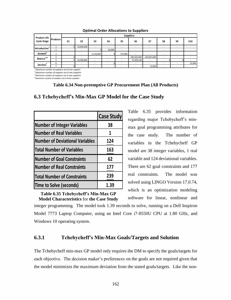
162
Table 6.34 Non-preemptive GP Procurement Plan (All Products)
6.3 Tchebycheff’s Min-Max GP Model for the Case Study
Table 6.35 provides information
regarding major Tchebycheff’s min-
max goal programming attributes for
the case study. The number of
variables in the Tchebycheff GP
model are 38 integer variables, 1 real
variable and 124 deviational variables.
There are 62 goal constraints and 177
real constraints. The model was
solved using LINGO Version 17.0.74,
which is an optimization modeling
software for linear, nonlinear and
integer programming. The model took 1.39 seconds to solve, running on a Dell Inspiron
Model 7773 Laptop Computer, using an Intel Core i7-8550U CPU at 1.80 GHz, and
Windows 10 operating system.
6.3.1 Tchebycheff’s Min-Max Goals/Targets and Solution
The Tchebycheff min-max GP model only requires the DM to specify the goals/targets for
each objective. The decision maker’s preferences on the goals are not required given that
the model minimizes the maximum deviation from the stated goals/targets. Like the non-
S1 S2 S3 S4 S5 S6 S7 S8 S9 S10
1 0 10,000,000 - - - - - - - -
2 - - 0 50,000 - - - - - -
Growth23 - - 2,276,004 0 723,996 - - - - -
4 0 - - - - 200,303,000 139,697,000 - - -
5 0 34,490,860 - - - 75,509,140 - 0 0 -
6 - - - 0 - - - - - 25,000
7 0 - - - - - 15,000 - -
4 Maximum number of suppliers set to three suppliers
Introduction1
Optimal Order Allocations to Suppliers
Product Life
Cycle StageProducts
Suppliers
Mature3,4
Decline2
1 Maximum number of suppliers set at one supplier2
Maximum number of suppliers set to two suppliers3
Minimum number of suppliers set to two suppliers
Case StudyNumber of Integer Variables 38
Number of Real Variables 1
Number of Deviational Variables 124
Total Number of Variables 163
Number of Goal Constraints 62
Number of Real Constraints 177
Total Number of Constraints 239
Time to Solve (seconds) 1.39
Table 6.35 Tchebycheff’s Min-Max GP
Model Characteristics for the Case Study

163
preemptive GP model, the target levels are set at 95% of the ideal values for maximization
and 105% of ideal values for minimization of the criteria. The Tchebycheff GP model
reduces to a single objective optimization model. The goal constraints must be normalized
or scaled to facilitate an equal comparison among the goal objectives. The optimal solution
to the Tchebycheff min-max GP model will be discussed next.
6.3.2 Introduction Phase Results (Product 1)
Table 6.36 displays the
procurement plan for product
1, in the introduction phase.
Supplier 2 is chosen to supply
the entire yearly demand. A
constraint limiting the
maximum number of suppliers
for the introduction phase to
one does not allow splitting the
demand between two suppliers. Table 6.37 presents the Tchebycheff goal achievements
for the supplier selection with respect to the target values. Supplier 2’s performance is
equal to or better than supplier 1’s performance in 8 of the 9 selection criteria. Supplier 1
only exceeds supplier 2 in the delivery performance rating. Therefore, the goal
achievements for product 1 exceed the target values in 7 of the 8 performance criteria (4.8%
S1 S2
0 10,000,000
1 Maximum number of suppliers set to one supplier
Optimal Order Allocations to SuppliersSuppliers
Order Allocations1
Selection Criteria
Target Values
(95% or 105%
of Ideals)
Goal
Achievements Target Achievement
Maximize Delivery Performance 90,250,000 90,000,000 Missed by 0.3%
Maximize Lead-Time Performance 85,500,000 90,000,000 Exceeded by 5.3%
Minimize Price 472,500 450,000 Exceeded by 4.8%
Maximize Tooling Development Time Performance 85,500,000 90,000,000 Exceeded by 5.3%
Maximize Service/Capacity Planning Performance 85,500,000 90,000,000 Exceeded by 5.3%
Maximize Product Performance 90,250,000 95,000,000 Exceeded by 5.3%
Maximize Product Safety Performance 95,000,000 100,000,000 Exceeded by 5.3%
Maximize Advanced Technology Rating 76,000,000 80,000,000 Exceeded by 5.3%
Maximize Quality Performance 90,250,000 95,000,000 Exceeded by 5.3%
Table 6.37 Tchebycheff’s GP Achievements for Introduction Phase Product 1 with
respect to Target Values
Table 6.36 Tchebycheff’s Min-Max GP Procurement
Plan for Introduction Phase Product 1

164
- 5.3%). Only the delivery performance goal is missed by 0.3%. Given the restriction of
selecting only 1 supplier, this solution provides overall better performance than the
alternative of selecting supplier 1 to fulfill the yearly demand.
6.3.3 Introduction Phase Results (Product 2)
Table 6.38 displays the
procurement plan for product
2, in the introduction phase.
Supplier 3 is chosen to supply
the entire yearly demand. The
constraint limiting the number
of suppliers for the
introduction phase to one does
not allow splitting the demand between two suppliers. Table 6.39 presents the Tchebycheff
goal achievements for the supplier selection criteria with respect to the target values.
Supplier 3’s performance is equal to supplier 4’s performance in 6 of the 9 performance
criteria resulting in the target values being exceeded by 5.3%. Supplier 3’s price
performance is also better than that of supplier 4, causing the price performance to surpass
the target by 4.8%. Safety and quality performance miss the target values by 6.4%, since
supplier 3’s performance is below supplier 4 in both of these criteria.
S3 S4
50,000 0
1 Maximum number of suppliers set to one supplier
Optimal Order Allocations to SuppliersSuppliers
Order Allocations1
Selection Criteria
Target Values
(95% or 105%
of Ideals)
Goal
Achievements Target Achievement
Maximize Delivery Performance 451,250 475,000 Exceeded by 5.3%
Maximize Lead-Time Performance 427,500 450,000 Exceeded by 5.3%
Minimize Price 91,350 87,000 Exceeded by 4.8%
Maximize Tooling Development Time Performance 380,000 400,000 Exceeded by 5.3%
Maximize Service/Capacity Planning Performance 380,000 400,000 Exceeded by 5.3%
Maximize Product Performance 427,500 450,000 Exceeded by 5.3%
Maximize Product Safety Performance 427,500 400,000 Missed by 6.4%
Maximize Advanced Technology Rating 380,000 400,000 Exceeded by 5.3%
Maximize Quality Performance 427,500 400,000 Missed by 6.4%
Table 6.39 Tchebycheff’s GP Achievements for Introduction Phase Product 2 with
respect to Target Values
Table 6.38 Tchebycheff’s Min-Max GP Procurement
Plan for Introduction Phase Product 2

165
6.3.4 Growth Phase Results (Product 3)
Table 6.40 displays the procurement plan for product 3, in the growth phase. Suppliers 3
and 5 are chosen to supply the yearly demand. A constraint limiting the maximum number
of suppliers for the growth phase product to two allows for splitting the demand between
two suppliers. Table 6.41 presents the Tchebycheff goal achievements for the supplier
selection with respect to target values. Suppliers 3, 4 and 5 have equal performance ratings
in 5 of the 8 selection criteria. This equal performance rating results in the target values
being exceeded by 5.3% for these criteria. Overall price performance surpasses the target
by 4.0%. The optimal solution allocates 92% of the yearly demand to supplier 3. This
results in both product safety and quality performance missing the target values by 5.6%,
given supplier 3 has the lowest performance rating in both of these criteria.
Table 6.41 Tchebycheff’s GP Achievements for Growth Phase Product 3 with
respect to Target Values
S3 S4 S5
2,777,995 0 222,005
Optimal Order Allocations to SuppliersSuppliers
Order Allocations1
1 Maximum number of suppliers set to two suppliers
Table 6.40 Tchebycheff’s Min-Max GP Procurement Plan for Growth Phase
Product 3

166
6.3.5 Mature Phase Results (Product 4)
Table 6.42 displays the procurement plan for product 4, in the mature phase. Suppliers 6
and 7 are chosen to supply the yearly demand. Table 6.43 presents the Tchebycheff goal
achievements for the supplier selection criteria with respect to the target values. Several
constraints impacted the selection of suppliers. The mature phase sets the minimum
number of required suppliers to two and the maximum number of suppliers to three. This
constraint supports the DM’s objective of creating price competition in order to improve
the gross margin for mature phase products.
The procurement plan for product 4 exceeds the target values for 8 of the 9 goal priorities
(Table 6.43). The excess target achievements range from 0.8% to 5.3%, with 6 of the 8
goal priorities exceeding by 5.3%. Supplier 6 is selected to supply 69% of the yearly
demand and has the highest criteria performance rankings in 8 of the 9 criteria, supporting
the target achievements. Product 4, which has a higher yearly demand of 340MM units,
achieves the price target supporting the decision maker’s goal of improving product gross
profit margin. It is important to note that these Tchebycheff min-max GP goal
achievements are accomplished without the use of a DM’s priority ranking or goal weights.
The only goal achievement, which misses the target value is tooling development time,
which misses the target by 6.9%. This miss is due to the selection of supplier 6, which has
a tooling score of 7, as compared to supplier 7, which has a tooling performance ranking
of 9.
S1 S6 S7
0 237,623,700 102,376,300 1 Minimum number of suppliers set to two suppliers
Optimal Order Allocations to SuppliersSuppliers
Order Allocations1,2
2 Maximum number of suppliers set to three suppliers
Table 6.42 Tchebycheff’s Min-Max GP Procurement Plan for Mature Phase
Product 4

167
Table 6.43 Tchebycheff’s GP Achievements for Mature Phase Product 4 with
respect to Target Values
6.3.6 Mature Phase Results (Product 5)
Table 6.44 displays the procurement plan for product 5, in the mature phase. Suppliers 2
and 6 are chosen to supply the yearly demand of 110MM units. Table 6.45 presents the
goal achievements for the supplier selection criteria with respect to the target values.
Product 5 also requires a minimum of two suppliers and a maximum of three suppliers to
enhance competition among the suppliers, supporting improved gross profit margins for
mature phase products.
The procurement plan for product 5 exceeds the target values in 7 out of 9 goal priorities
(Table 6.45). The excess target achievements range from 0.8% to 5.3%, with 6 out of 7
goal priorities exceeding by 5.3%. Supplier 2 is selected to supply 47% of the yearly
demand. The selection of supplier 2 has a negative impact on price performance, which
recorded a target miss of 7.0%. This 7.0% target miss is the maximum miss for all product
Table 6.44 Tchebycheff’s Min-Max GP Procurement Plan for Mature Phase
Product 5

168
life cycle phases and products. Tooling development time performance also misses the
target by 6.9%, due supplier 6’s performance rating. While supplier 6 has the best price
performance rating, the poor tooling development time contributed to the 6.9% target miss.
It should be noted that the price performance does not meet the DM’s objectives of
improving price performance for mature products. This result is not unexpected given
Tchebycheff GP’s min-max criterion, which does not use any decision maker’s input and
simply minimizes the maximum deviation from the target values.
6.3.7 Decline Phase Results (Product 6)
Table 6.46 displays the
procurement plan for product 6,
in the decline phase. Both
supplier 4 and 10 are selected to
supply 45% and 55% of the
yearly demand respectively.
Table 6.47 presents the
Tchebycheff min-max goal
achievements for the supplier selection criteria with respect to the target values.
S4 S10
11,198 13,802
Optimal Order Allocations to SuppliersSuppliers
Order Allocations1
1 Maximum number of suppliers set to two suppliers
Selection Criteria
Target Values
(95% or 105%
of Ideals)
Goal
Achievements Target Achievement
Maximize Delivery Performance 982,300,000 990,000,000 Exceeded by 0.8%
Maximize Lead-Time Performance 940,500,000 990,000,000 Exceeded by 5.3%
Minimize Price 4,435,200 4,744,782 Missed by 7.0%
Maximize Tooling Development Time Performance 940,500,000 875,268,460 Missed by 6.9%
Maximize Service/Capacity Planning Performance 940,500,000 990,000,000 Exceeded by 5.3%
Maximize Product Performance 992,750,000 1,045,000,000 Exceeded by 5.3%
Maximize Product Safety Performance 1,045,000,000 1,100,000,000 Exceeded by 5.3%
Maximize Past Performance 940,500,000 990,000,000 Exceeded by 5.3%
Maximize Quality Performance 992,750,000 1,045,000,000 Exceeded by 5.3%
Table 6.45 Tchebycheff’s GP Achievements for Mature Phase Product 5 with
respect to Target Values
Table 6.46 Tchebycheff’s Min-Max GP
Procurement Plan for Decline Phase Product 6

169
The procurement plan for product 6 exceeds or achieves the target values in 6 of 9 goal
priorities (Table 6.47). The excess target achievements range from 0% to 5.3%. Splitting
the demand between two suppliers negatively impacts all of the performance criteria,
excluding the service and capacity planning and past performance criteria. Supplier
performance is equal for both of these criteria. The performance target misses are lead-
time by 1.2%, delivery by 3.9% and price by 6.9%. The price target miss of 6.9% nearly
matches the maximum overall miss of 7.0%, which is related to mature phase product 5’s
price performance (see Table 6.45). The optimal solution divides the yearly demand
between the two suppliers, while achieving the overall minimization of the maximum
deviation from the target values.
Selection Criteria
Target Values
(95% or 105%
of Ideals)
Goal
Achievements Target Achievement
Maximize Delivery Performance 225,625 216,797 Missed by 3.9%
Maximize Lead-Time Performance 213,750 211,198 Missed by 1.2%
Minimize Price 107,100 114,542 Missed by 6.9%
Maximize Tooling Development Time Performance 213,750 213,802 Achieved Target
Maximize Service/Capacity Planning Performance 190,000 200,000 Exceeded by 5.3%
Maximize Product Performance 225,625 231,901 Exceeded by 2.8%
Maximize Product Safety Performance 237,500 238,802 Exceeded by 0.5%
Maximize Past Performance 190,000 200,000 Exceeded by 5.3%
Maximize Quality Performance 225,625 231,901 Exceeded by 2.8%
Table 6.47 Tchebycheff’s GP Achievements for Decline Phase Product 6 with
respect to Target Values
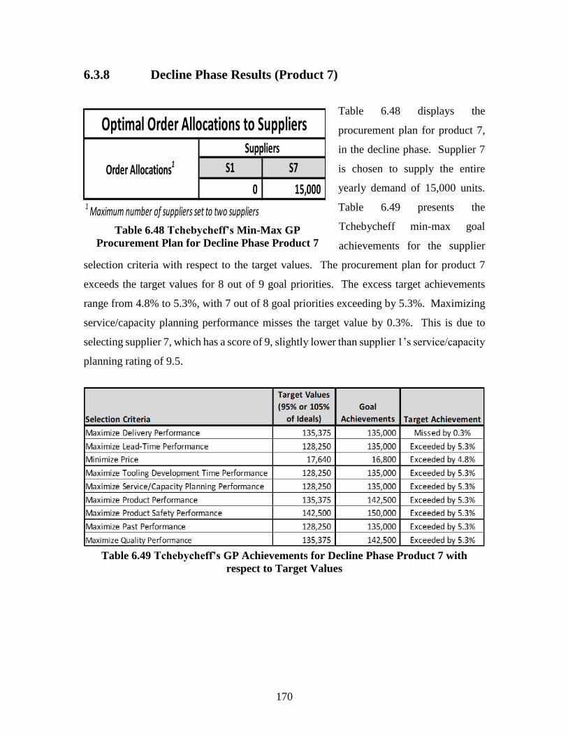
170
6.3.8 Decline Phase Results (Product 7)
Table 6.48 displays the
procurement plan for product 7,
in the decline phase. Supplier 7
is chosen to supply the entire
yearly demand of 15,000 units.
Table 6.49 presents the
Tchebycheff min-max goal
achievements for the supplier
selection criteria with respect to the target values. The procurement plan for product 7
exceeds the target values for 8 out of 9 goal priorities. The excess target achievements
range from 4.8% to 5.3%, with 7 out of 8 goal priorities exceeding by 5.3%. Maximizing
service/capacity planning performance misses the target value by 0.3%. This is due to
selecting supplier 7, which has a score of 9, slightly lower than supplier 1’s service/capacity
planning rating of 9.5.
S1 S7
0 15,000
Optimal Order Allocations to SuppliersSuppliers
Order Allocations1
1 Maximum number of suppliers set to two suppliers
Table 6.48 Tchebycheff’s Min-Max GP
Procurement Plan for Decline Phase Product 7
Table 6.49 Tchebycheff’s GP Achievements for Decline Phase Product 7 with
respect to Target Values

171
6.3.9 Optimal Order Allocations to Suppliers (All Products)
The previous sections have reviewed the detailed order allocations and goal achievements
versus the target values by PLC phase and product. Table 6.50 presents the over-all
procurement plan for all products by the Tchebycheff’s min-max GP model. The optimal
procurement plan demonstrates the key characteristic of the Tchebycheff min-max goal
methodology, which is the minimization of the maximum deviation from the target
values.
The maximum deviation from the targets for the Tchebycheff min-max GP model is a
7.0%, which is related to mature product 5’s price performance. This 7.0% target miss is
less than the maximum target misses from both the preemptive and non-preemptive
models, which are 29.8% and 11.4% respectively. While the target miss of 7.0% does
not meet the DM’s objectives by of improving gross margin for mature products, this
result clearly illustrates the objective of minimizing the maximum deviation from the
target values without any DM’s input.
S1 S2 S3 S4 S5 S6 S7 S8 S9 S10
1 0 10,000,000 - - - - - - - -
2 - - 50,000 0 - - - - - -
Growth23 - - 2,777,995 0 222,005 - - - - -
4 0 - - - - 237,623,700 102,376,300 - - -
5 0 52,634,230 - - - 57,365,770 - 0 0 -
6 - - - 11,198 - - - - - 13,802
7 0 - - - - - 15,000 - -
4 Maximum number of suppliers set to three suppliers
Introduction1
Optimal Order Allocations to Suppliers
Product Life
Cycle StageProducts
Suppliers
Mature3,4
Decline2
1 Maximum number of suppliers set at one supplier2
Maximum number of suppliers set to two suppliers3
Minimum number of suppliers set to two suppliers
Table 6.50 Tchebycheff’s Min-Max GP Procurement Plan (All Products)

172
6.4 Fuzzy Min-Max GP Model for the Case Study
Table 6.51 provides information
regarding major fuzzy min-max
goal programming attributes for
the case study. The number of
variables in the fuzzy GP model
are 38 integer variables, 1 real
variable and 124 deviational
variables. There are 62 goal
constraints and 177 real
constraints. The model was
solved using LINGO Version
17.0.74, which is an optimization
modeling software for linear, nonlinear and integer programming. The model took 1.82
seconds to solve, running on a Dell Inspiron Model 7773 Laptop Computer, using an Intel
Core i7-8550U CPU at 1.80 GHz, and Windows 10 operating system.
6.4.1 Fuzzy Min-Max Ideals and Solution
The fuzzy min-max GP model does not require any inputs from the DM, since the ideal
values are used as the targets for each objective. The decision maker’s preferences on the
objectives are not required given that the model minimizes the maximum deviation from
the ideal values. Recall that the ideal values are the maximum/minimum values for each
objective, depending on whether the objective is to maximize/minimize. The fuzzy GP
model reduces to a single objective optimization model. The goal constraints must be
normalized or scaled to facilitate an equal comparison among the goal objectives. Results
from the fuzzy GP model provide a benchmark to compare the results based on the ideal
solution versus the DM’s target values, which are used in preemptive, non-preemptive and
Tchebycheff’s min-max models. The optimal solution to the fuzzy min-max GP model will
be discussed next.
Case StudyNumber of Integer Variables 38
Number of Real Variables 1
Number of Deviational Variables 124
Total Number of Variables 163
Number of Goal Constraints 62
Number of Real Constraints 177
Total Number of Constraints 239
Time to Solve (seconds) 1.82Table 6.51 Fuzzy Min-Max GP Model
Characteristics for the Case Study

173
6.4.2 Introduction Phase Results (Product 1)
Table 6.52 displays the
procurement plan for product 1, in
the introduction phase. Supplier 2
is chosen to supply the entire
yearly demand. A constraint
limiting the maximum number of
suppliers for the introduction
phase to one does not allow
splitting the demand between two suppliers. Table 6.53 presents the fuzzy GP criteria
achievements with respect to the ideal values. Supplier 2’s performance is equal to or
better than supplier 1’s performance in 8 of the 9 selection criteria. Supplier 1 only exceeds
supplier 2 in the delivery performance rating. Therefore, the goal achievements for product
1 achieve the ideal values in 7 of the 8 performance criteria. Only the ideal delivery target
is missed by 5.3%. Given the restriction of selecting only 1 supplier, this solution provides
overall better performance than the alternative of selecting supplier 1 to fulfill the yearly
demand.
S1 S2
0 10,000,000
1 Maximum number of suppliers set to one supplier
Optimal Order Allocations to SuppliersSuppliers
Order Allocations1
Table 6.52 Fuzzy Min-Max GP Procurement Plan
for Introduction Phase Product 1
Table 6.53 Fuzzy GP Achievements for Introduction Phase Product 1 with respect
to Ideal Values

174
6.4.3 Introduction Phase Results (Product 2)
Table 6.54 displays the
procurement plan in the
introduction phase for product
2. Supplier 3 was chosen to
supply the entire yearly
demand. Table 6.55 presents
the fuzzy GP criteria
achievements with respect to
the ideal values. Supplier 3 is chosen to supply the entire yearly demand. The constraint
limiting the maximum number of suppliers for the introduction phase to one does not allow
splitting the demand between two suppliers. Except for safety and quality performance,
all the supplier performance criteria achieve the ideal values. Both safety and quality miss
the ideal values by 11.1%. This illustrates the logic of the fuzzy GP model, which
determines an optimal solution based on minimizing the maximum deviation from the ideal
values.
S3 S4
50,000 0
1 Maximum number of suppliers set to one supplier
Optimal Order Allocations to SuppliersSuppliers
Order Allocations1
Selection Criteria Ideal Values Criteria Values
Criteria
Achievements
Maximize Delivery Performance 475,000 475,000 Achieved Ideal
Maximize Lead-Time Performance 450,000 450,000 Achieved Ideal
Minimize Price 87,000 87,000 Achieved Ideal
Maximize Tooling Development Time Performance 400,000 400,000 Achieved Ideal
Maximize Service/Capacity Planning Performance 400,000 400,000 Achieved Ideal
Maximize Product Performance 450,000 450,000 Achieved Ideal
Maximize Product Safety Performance 450,000 400,000 Missed by 11.1%
Maximize Advanced Technology Rating 400,000 400,000 Achieved Ideal
Maximize Quality Performance 450,000 400,000 Missed by 11.1%
Table 6.54 Fuzzy GP Procurement Plan for
Introduction Phase Product 2
Table 6.55 Fuzzy GP Achievements for Introduction Phase Product 2 with respect
to Ideal Values

175
6.4.4 Growth Phase Results (Product 3)
Table 6.56 displays the procurement plan for product 3, in the growth phase. Suppliers 3
and 5 are chosen to supply the yearly demand. A constraint limiting the maximum number
of suppliers for the growth product to two allows for the splitting of the demand between
two suppliers. Table 6.57 presents the fuzzy GP criteria achievements with respect to the
ideal values. The procurement plan for product 3 achieves the ideal values for 5 out of 8
supplier criteria. Price, safety and quality miss the ideal values by 2.7%, 8.4% and 8.4%
respectively. The safety and quality performance of supplier 3 is below those of both
supplier 4 and 5, which explains the failure to achieve the ideal values. While supplier 3
has the best price, the choice of supplier 5 to supply nearly 32% of the yearly demand
degrades the price performance. It should be noted that the DM ranked growth phase
quality and safety (see Table 6.2) as the highest priorities for the preemptive GP model.
The fuzzy GP does not consider DM’s inputs and generates the optimal solution by simply
minimizing the maximum deviation from the ideal values!
S3 S4 S5
2,276,004 0 723,996
Optimal Order Allocations to SuppliersSuppliers
Order Allocations1
1 Maximum number of suppliers set to two suppliers
Selection Criteria Ideal Values Criteria Values
Criteria
Achievements
Maximize Delivery Performance 28,500,000 28,500,000 Achieved Ideal
Maximize Lead-Time Performance 27,000,000 27,000,000 Achieved Ideal
Minimize Price 26,040,000 26,742,276 Missed by 2.7%
Maximize Tooling Development Time Performance 24,000,000 24,000,000 Achieved Ideal
Maximize Service/Capacity Planning Performance 24,000,000 24,000,000 Achieved Ideal
Maximize Product Performance 27,000,000 27,000,000 Achieved Ideal
Maximize Product Safety Performance 27,000,000 24,723,996 Missed by 8.4%
Maximize Quality Performance 27,000,000 24,723,996 Missed by 8.4%
Table 6.56 Fuzzy GP Procurement Plan for Growth Phase Product 3
Table 6.57 Fuzzy GP Achievements for Growth Phase Product 3 with respect to
Ideal Values
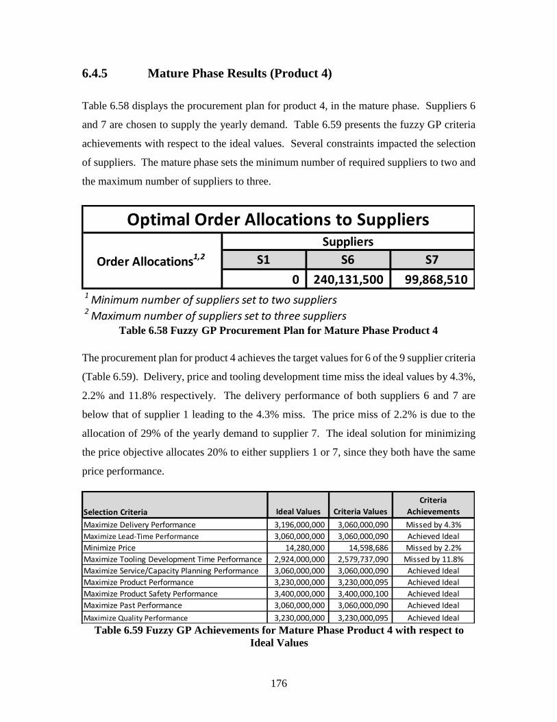
176
6.4.5 Mature Phase Results (Product 4)
Table 6.58 displays the procurement plan for product 4, in the mature phase. Suppliers 6
and 7 are chosen to supply the yearly demand. Table 6.59 presents the fuzzy GP criteria
achievements with respect to the ideal values. Several constraints impacted the selection
of suppliers. The mature phase sets the minimum number of required suppliers to two and
the maximum number of suppliers to three.
The procurement plan for product 4 achieves the target values for 6 of the 9 supplier criteria
(Table 6.59). Delivery, price and tooling development time miss the ideal values by 4.3%,
2.2% and 11.8% respectively. The delivery performance of both suppliers 6 and 7 are
below that of supplier 1 leading to the 4.3% miss. The price miss of 2.2% is due to the
allocation of 29% of the yearly demand to supplier 7. The ideal solution for minimizing
the price objective allocates 20% to either suppliers 1 or 7, since they both have the same
price performance.
S1 S6 S7
0 240,131,500 99,868,510 1 Minimum number of suppliers set to two suppliers
Optimal Order Allocations to SuppliersSuppliers
Order Allocations1,2
2 Maximum number of suppliers set to three suppliers
Selection Criteria Ideal Values Criteria Values
Criteria
Achievements
Maximize Delivery Performance 3,196,000,000 3,060,000,090 Missed by 4.3%
Maximize Lead-Time Performance 3,060,000,000 3,060,000,090 Achieved Ideal
Minimize Price 14,280,000 14,598,686 Missed by 2.2%
Maximize Tooling Development Time Performance 2,924,000,000 2,579,737,090 Missed by 11.8%
Maximize Service/Capacity Planning Performance 3,060,000,000 3,060,000,090 Achieved Ideal
Maximize Product Performance 3,230,000,000 3,230,000,095 Achieved Ideal
Maximize Product Safety Performance 3,400,000,000 3,400,000,100 Achieved Ideal
Maximize Past Performance 3,060,000,000 3,060,000,090 Achieved Ideal
Maximize Quality Performance 3,230,000,000 3,230,000,095 Achieved Ideal
Table 6.58 Fuzzy GP Procurement Plan for Mature Phase Product 4
Table 6.59 Fuzzy GP Achievements for Mature Phase Product 4 with respect to
Ideal Values

177
The highest miss of 11.8% for tooling development time is due to the allocation of nearly
70.5% of the yearly demand to supplier 6, which has a second best tooling development
time performance with supplier 7 having the best performance. This 11.8% miss is tied for
the maximum deviation from the ideal solutions in the fuzzy GP model.
6.4.6 Mature Phase Results (Product 5)
Table 6.60 displays the procurement plan for product 5, in the mature phase. Suppliers 2
and 6 were chosen to supply the expected yearly demand of 110MM units. Table 6.61
presents the fuzzy GP criteria achievements with respect to the ideal values. Product 5 also
requires a minimum of two suppliers and a maximum of three suppliers to enhance
competition among the suppliers, supporting improved gross profit margins for mature
phase products.
The procurement plan for product 5 achieves the ideal values for 6 of the 9 supplier
objectives (Table 6.61). Delivery, price and tooling development time miss the ideal values
by 4.3%, 11.8% and 11.8% respectively. The delivery performance of both suppliers 2 and
6 are below that of supplier 1, leading to the 4.3% miss. The price miss of 11.8%, which
matches the maximum deviation from the ideal solution, is due to the allocation of only
58.7% of the yearly demand to supplier 6. The ideal solution that minimizes prices
allocates 80% to supplier 6.
S1 S2 S6 S8 S9
0 51,390,730 58,609,270 0 0
Optimal Order Allocations to SuppliersSuppliers
Order Allocations1,2
1 Minimum number of suppliers set to two suppliers2 Maximum number of suppliers set to three suppliers
Table 6.60 Fuzzy GP Procurement Plan for Mature Phase Product 5
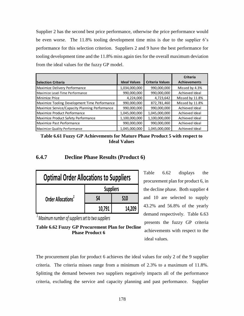
178
Supplier 2 has the second best price performance, otherwise the price performance would
be even worse. The 11.8% tooling development time miss is due to the supplier 6’s
performance for this selection criterion. Suppliers 2 and 9 have the best performance for
tooling development time and the 11.8% miss again ties for the overall maximum deviation
from the ideal values for the fuzzy GP model.
6.4.7 Decline Phase Results (Product 6)
Table 6.62 displays the
procurement plan for product 6, in
the decline phase. Both supplier 4
and 10 are selected to supply
43.2% and 56.8% of the yearly
demand respectively. Table 6.63
presents the fuzzy GP criteria
achievements with respect to the
ideal values.
The procurement plan for product 6 achieves the ideal values for only 2 of the 9 supplier
criteria. The criteria misses range from a minimum of 2.3% to a maximum of 11.8%.
Splitting the demand between two suppliers negatively impacts all of the performance
criteria, excluding the service and capacity planning and past performance. Supplier
S4 S10
10,791 14,209
Optimal Order Allocations to SuppliersSuppliers
Order Allocations1
1 Maximum number of suppliers set to two suppliers
Selection Criteria Ideal Values Criteria Values
Criteria
Achievements
Maximize Delivery Performance 1,034,000,000 990,000,000 Missed by 4.3%
Maximize Lead-Time Performance 990,000,000 990,000,000 Achieved Ideal
Minimize Price 4,224,000 4,723,642 Missed by 11.8%
Maximize Tooling Development Time Performance 990,000,000 872,781,460 Missed by 11.8%
Maximize Service/Capacity Planning Performance 990,000,000 990,000,000 Achieved Ideal
Maximize Product Performance 1,045,000,000 1,045,000,000 Achieved Ideal
Maximize Product Safety Performance 1,100,000,000 1,100,000,000 Achieved Ideal
Maximize Past Performance 990,000,000 990,000,000 Achieved Ideal
Maximize Quality Performance 1,045,000,000 1,045,000,000 Achieved Ideal
Table 6.61 Fuzzy GP Achievements for Mature Phase Product 5 with respect to
Ideal Values
Table 6.62 Fuzzy GP Procurement Plan for Decline
Phase Product 6

179
performance is equal for both of these criteria. The criteria misses are delivery by 9.0%,
lead-time by 6.3%, price by 11.8%, tooling development time by 4.8%, product
performance by 2.3%, product safety by 4.3% and quality by 2.3%. The price miss matches
the maximum overall fuzzy GP miss of 11.8%. The optimal solution divides the yearly
demand between the two suppliers, while achieving the overall minimization of the
maximum deviation from the ideal values.
6.4.8 Decline Phase Results (Product 7)
Table 6.64 displays the
procurement plan for product 7,
in the decline phase. Supplier 7
is chosen to supply the entire
yearly demand of 15,000 units.
Table 6.65 presents the fuzzy GP
criteria achievements with
respect to the ideal values.
S1 S7
0 15,000
Optimal Order Allocations to SuppliersSuppliers
Order Allocations1
1 Maximum number of suppliers set to two suppliers
Selection Criteria Ideal Values Criteria Values
Criteria
Achievements
Maximize Delivery Performance 237,500 216,187 Missed by 9.0%
Maximize Lead-Time Performance 225,000 210,791 Missed by 6.3%
Minimize Price 102,000 114,086 Missed by 11.8%
Maximize Tooling Development Time Performance 225,000 214,209 Missed by 4.8%
Maximize Service/Capacity Planning Performance 200,000 200,000 Achieved Ideal
Maximize Product Performance 237,500 232,105 Missed by 2.3%
Maximize Product Safety Performance 250,000 239,209 Missed by 4.3%
Maximize Past Performance 200,000 200,000 Achieved Ideal
Maximize Quality Performance 237,500 232,105 Missed by 2.3%
Table 6.63 Fuzzy GP Achievements for Mature Phase Product 6 with respect to
Ideal Values
Table 6.64 Fuzzy GP Procurement Plan for Decline
Phase Product 7

180
The procurement plan for product 7 achieves the ideal values for 8 out of 9 supplier criteria.
Only the delivery performance misses the ideal value by 5.3%. Missing this target is due
to selecting supplier 7, which has a score of 9, slightly lower than supplier 1’s delivery
performance rating of 9.5.
6.4.9 Optimal Order Allocations to Suppliers (All Products)
The previous sections have reviewed the detailed order allocations and criteria
achievements with respect to the ideal values by PLC phase and product. Table 6.66
presents the over-all procurement plan for all products by the fuzzy min-max GP model.
The optimal procurement plan demonstrates the key characteristic of the fuzzy GP, which
is the minimization of the maximum deviation from the ideal values without any input from
the decision makers.
The optimal solution for the fuzzy model achieves 67.7% of the ideal values (see Figure
6.1). The ideal value misses range from 2.2% to 11.8%, with a median value of 5.8%. The
maximum deviations of 11.8% are related to mature product 4 tooling development time,
mature product 5 price, mature product 5 tooling development time and decline product 6
price performance. While these price ideal misses do not meet the DM’s objectives of
improving gross margin for mature products by improving price performance, they
Selection Criteria Ideal Values Criteria Values
Criteria
Achievements
Maximize Delivery Performance 142,500 135,000 Missed by 5.3%
Maximize Lead-Time Performance 135,000 135,000 Achieved Ideal
Minimize Price 16,800 16,800 Achieved Ideal
Maximize Tooling Development Time Performance 135,000 135,000 Achieved Ideal
Maximize Service/Capacity Planning Performance 135,000 135,000 Achieved Ideal
Maximize Product Performance 142,500 142,500 Achieved Ideal
Maximize Product Safety Performance 150,000 150,000 Achieved Ideal
Maximize Past Performance 135,000 135,000 Achieved Ideal
Maximize Quality Performance 142,500 142,500 Achieved Ideal
Table 6.65 Fuzzy GP Achievements for Decline Phase Product 7 with respect to
Ideal Values

181
represent the optimal fuzzy GP logic. These results should not be a surprise given the fuzzy
GP’s objective of minimizing the maximum deviation from the ideal values without any
DM’s input. A direct comparison of the fuzzy GP model results to the preemptive, non-
preemptive and Tchebycheff min-max model results is not appropriate, since no targets
specified by the DMs are used in the fuzzy GP. However, the fuzzy GP results do provide
an insight into the ideal criteria achievements without any DM input.
Figure 6.1 Fuzzy GP Results
Table 6.66 Fuzzy Min-Max GP Procurement Plan (All Products)

182
6.5 Value Path Results
This section reviews the overall model results by product life cycle phase and product using
the Value Path approach discussed in Ravindran and Warsing (2013). The Value Path
approach allows the DM to view the results and various tradeoffs in a complex model by
displaying the results as a set of parallel scales. This graphical display allows the decision
makers to choose the best-compromise solution. Value Path results by product life cycle
phase and product for the Tchebycheff, non-preemptive and preemptive models will be
discussed. The fuzzy GP model results will not be included in this section, since no targets
specified by the DMs are used in the fuzzy GP. Fuzzy GP results are based on achievement
of the ideal values versus the Tchebycheff non-preemptive and preemptive models which
use decision maker specified target values.
6.5.1 Introduction Phase (Product 1)
Table 6.67 displays the
procurement plan by GP model
for product 1, in the introduction
phase. A constraint limiting the
maximum number of suppliers
for the introduction phase to one
does not allow splitting the
demand between the two
suppliers. Supplier 2 is chosen to
supply the entire yearly demand
of 10 MM units for both the
Tchebycheff min-max and non-
preemptive GP models. Selecting supplier 1 to provide the total yearly demand is the
optimal solution for the preemptive GP model. Table 6.68 presents the target values and
goal achievements for each of the goal programming models. The goals are listed in the
preemptive GP goal priority order (see Table 6.2). These goal priorities are directly related
to the criteria weights utilized by the non-preemptive GP model (see Table 6.19). The goal
S1 S2
Tchebycheff's Min/Max 0 10,000,000
Non-preemptive 0 10,000,000
Preemptive 10,000,000 0
1 Maximum number of suppliers set to one supplier
Optimal Order Allocations1 to Suppliers
by GP ModelSuppliers
GP Model
Table 6.67 Procurement Plan by GP Model for
Introduction Phase Product 1

183
priority order or goal weights are not relevant to Tchebycheff’s min-max model, which
minimizes the maximum deviation from the target values without any DM input.
These model results, representing the goal achievements for product 1, are normalized.
This normalization of the goal achievements is accomplished by dividing each achieved
goal constraint solution by the best achieved goal constraint solution for minimizing
objectives. For the maximizing objectives, the normalization is done by dividing the
maximum achieved value by the value obtained by each GP model. For example, in Table
6.68, for the Priority 8 goal, “Maximize Delivery Performance”, for product 1, the highest
value is 95,000,000. Hence the normalized values for the three GP models are
(95,000,000/90,000,000; 95,000,000/90,000,000; 95,000,000/95,000,000) or (1.05556,
1.0556, 1.00000). Similarly, in Table 6.68, for Priority 17 goal, “Minimize Price” for
introduction phase, the highest value is 450,000. Hence the normalized values are
(450,000/450,000; 450,000/450,000; 500,000/450,000) = (1.00000, 1.00000, 1.11111).
Thus, the best achievement for a specific goal constraint equals 1.0 with higher values
being less desirable. These models use the same target values (95% for maximization and
105% for minimization objectives) making the Value Path approach a viable method to
compare the GP model results. The fuzzy GP model results are excluded from the Value
Path analysis since the fuzzy model uses the ideal values as targets for the goal constraints.
Table 6.69 displays the normalized goal achievements for product 1.
Table 6.68 Model Results and Target Values for Introduction Phase Product 1

184
Figure 6.2 displays the Value Path graph for product 1 using the results of Table 6.68. The
results for product safety and quality are equal for all three GP models. However, the
delivery results for the Tchebycheff and non-preemptive models are worse compared to
the results of the preemptive model by 5.6%. Product performance is equal for all three
models. The goal attainments for preemptive GP model for all for the remaining priorities
are worse than those of the Tchebycheff and non-preemptive models. These poor goal
performances are for price, advanced technology, lead-time, service and capacity planning
and tooling development time with misses of 11.1%, 13.3%, 12.5%, 12.5% and 50%
respectively. The Value Path graph provides a clear picture of the disparities in goal
achievements by the three models and the results of the actual order allocations to the DMs.
During the review of the supplier selection results, the decision makers commented that
the tradeoff of 5.6% in delivery performance maybe considered in order to improve the
remaining goals performance. These comments present the power of the Value Path
method in comparing alternative solutions and performance tradeoffs.
Preemptive GP Supplier Goal Priority Order (Pi )
Tchebycheff's
Min/Max Results
Non-Preemptive
Results
Preemptive
Results
3.0 Maximize Product Safety 1.00000 1.00000 1.00000
7.0 Maximize Quality 1.00000 1.00000 1.00000
8.0 Maximize Delivery Performance 1.05556 1.05556 1.00000
9.0 Maximize Product Performance 1.00000 1.00000 1.00000
17.0 Minimize Price 1.00000 1.00000 1.11111
19.0 Maximize Advanced Technology 1.00000 1.00000 1.33333
20.0 Maximize Lead-time Performance 1.00000 1.00000 1.12500
21.0 Maximize Service Cap. Planning 1.00000 1.00000 1.12500
24.0 Maximize Tooling Dev. Time Performance 1.00000 1.00000 1.50000
Table 6.69 Value Path Results for Introduction Phase Product 1

185
6.5.2 Introduction Phase (Product 2)
Table 6.70 displays the
procurement plan by GP model
for product 2, in the introduction
phase. A constraint limiting the
maximum number of suppliers
for the introduction phase to one
does not allow splitting the
demand between the two
suppliers. Supplier 3 is chosen to
supply the entire yearly demand of
50,000 units for both the
Tchebycheff min-max and preemptive GP models. The optimal solution for the non-
preemptive model selects supplier 4 to provide the total yearly demand. Table 6.71
presents the target values and goal achievements for each of the goal programming models.
S3 S4
Tchebycheff's Min/Max 50,000 0
Non-preemptive 0 50,000
Preemptive 50,000 0
1 Maximum number of suppliers set to one supplier
Optimal Order Allocations1 to Suppliers
by GP ModelSuppliers
GP Model
Figure 6.2 Value Path Model Results Comparison for Introduction Phase Product 1
Table 6.70 Procurement Plan by GP Model for
Introduction Phase Product 2

186
The goals are listed in the preemptive GP goal priority order (see Table 6.2). These goal
priorities are directly related to the criteria weights utilized by the non-preemptive GP
model (see Table 6.19). The goal priority order or goal weights are not relevant to
Tchebycheff’s min-max model, which minimizes the maximum deviation from the target
values without any DM input.
Table 6.72 summarizes the normalized goal achievements for product 2 using the same
procedure described for product 1. Figure 6.3 displays the Value Path graph for product 2.
Examining the Value Path graph and Table 6.72, reveals the preemptive and Tchebycheff
GP models have worse performance than the non-preemptive GP model for product safety
and quality. These results may seem surprising given the high goal priorities for product
Preemptive GP Supplier Goal Priority Order (Pi )
Tchebycheff's
Min/Max Results
Non-
Preemptive
Results
Preemptive
Results
3.0 Maximize Product Safety 1.12500 1.00000 1.12500
7.0 Maximize Quality 1.12500 1.00000 1.12500
8.0 Maximize Delivery Performance 1.00000 1.00000 1.00000
9.0 Maximize Product Performance 1.00000 1.00000 1.00000
17.0 Minimize Price 1.00000 1.14943 1.00000
19.0 Maximize Advanced Technology 1.00000 1.00000 1.00000
20.0 Maximize Lead-time Performance 1.00000 1.00000 1.00000
21.0 Maximize Service Cap. Planning 1.00000 1.00000 1.00000
24.0 Maximize Tooling Dev. Time Performance 1.00000 1.00000 1.00000
Table 6.71 Model Results and Target Values for Introduction Phase Product 2
Table 6.72 Value Path Results for Introduction Phase Product 2

187
safety and quality of 3 and 7 respectively. Detailed testing of the model discovered the
achievement of goal priorities 1 and 2 for growth phase product 3, have a direct impact on
the supplier selection and order allocation of product 2. Despite supplier 4 having the best
performance rating with respect to safety and quality, supplier 3 was selected. Supplier 4
was chosen to supply 1.6 million units of product 3, which consumes the entire capacity of
supplier 4 with respect to business volume levels. This business volume constraint
combined with the best performance with respect to quality and safety required the
selection of supplier 4 for product 3. Achieving these higher priority goals was again done
at the detriment of the lower priority goals. This real-world example clearly demonstrates
the principles of preemptive goal programming. The non-preemptive GP model results are
equal to or better than the preemptive and Tchebycheff GP model results in all goal
priorities except price, which misses by 14.9%.
The decision makers were presented with a tradeoff between safety and quality
performance versus price. Another consideration discussed by the DMs was to relax the
business volume constraint on supplier 4, allowing a higher overall volume to be purchased
Figure 6.3 Value Path Model Results Comparison for Introduction Phase Product 2

188
from supplier 4. This relaxation of the business volume constraint could substantially
change the models results and require retesting in order to generate the new optimal
solutions for all the GP models. This discussion demonstrates the positive attributes of the
Value Path graph, which provides a clear picture of the tradeoffs among the conflicting
criteria.
6.5.3 Growth Phase (Product 3)
Table 6.73 displays the procurement plan by GP model for product 3, in the growth phase.
Suppliers 3 and 5 were chosen to supply the yearly demand for both the Tchebycheff and
non-preemptive GP models. Suppliers 3 and 4 where selected to supply the yearly demand
for the preemptive model. A constraint limiting the maximum number of suppliers for the
growth phase to two allows splitting the demand between the two suppliers. Table 6.74
presents the target values and goal achievements for each of the goal programming models.
The goals are listed in the preemptive GP goal priority order (see Table 6.2). These goal
priorities are directly related to the criteria weights utilized by the non-preemptive GP
model (see Table 6.19). The goal priority order or goal weights are not relevant to
Tchebycheff’s min-max model, which minimizes the maximum deviation from the target
values without any DM input.
S3 S4 S5
Tchebycheff's Min/Max 2,777,995 0 222,005
Non-preemptive 2,276,004 0 723,996
Preemptive 1,400,000 1,600,000 0
Optimal Order Allocations1 to Suppliers by GP
ModelSuppliers
1 Maximum number of suppliers set to two suppliers
GP Model
Table 6.73 Procurement Plan by GP Model for Growth Phase Product 3

189
Table 6.75 summarizes the normalized goal achievements for the product 3. Figure 6.4
displays the Value Path graph for product 3. Examining the Value Path graph and Table
6.75 reveals the Tchebycheff and non-preemptive GP models have worse performance than
the preemptive model for both quality and safety missing by 5.7% and 3.5% respectively
for both quality and safety. These goal performance differences should not be a surprise
give n that quality and safe ty are the highest ranked goals in the preemptive goal
programming model. All the models perform equally well for the delivery, lead-time,
service and capacity planning, product performance and tooling development time goals.
The preemptive GP misses price by 7.2%, while the non-preemptive model misses price
by 1.8%.
Preemptive GP Supplier Goal Priority Order (Pi )
Tchebycheff's
Min/Max Results
Non-
Preemptive
Results
Preemptive
Results
1.0 Maximize Quality 1.05689 1.03543 1.00000
2.0 Maximize Product Safety 1.05689 1.03543 1.00000
6.0 Maximize Delivery Performance 1.00000 1.00000 1.00000
10.0 Maximzie Leadtime Performance 1.00000 1.00000 1.00000
11.0 Maximize Service Cap. Planning 1.00000 1.00000 1.00000
12.0 Maximize Product Performance 1.00000 1.00000 1.00000
13.0 Minimize Price 1.00000 1.01855 1.07224
22.0 Maximize Tooling Dev. Time Performance 1.00000 1.00000 1.00000
Table 6.74 Model Results and Target Values for Growth Phase Product 3
Table 6.75 Value Path Results for Growth Phase Product 3

190
The results of the growth phase models present the DMs with a number of alternative
solutions and results. Quality and safety performance can be maximized by choosing the
preemptive GP solution understanding that price will miss the best solution by 7.2%.
Selecting the Tchebycheff model solution will yield the best price performance, but also
the worst performance with respect to quality and safety. Once again, the Value Path graph
clearly presents the solutions results and tradeoffs visually for the goal priorities.
6.5.4 Mature Phase (Product 4)
Table 6.76 displays the procurement plan by GP model for product 4, in the mature phase.
Suppliers 6 and 7 were chosen to supply the yearly demand for all of the GP models with
order allocations varying by model. Several constraints impacted the selection of
suppliers. The mature phase sets the minimum number of required suppliers to two and
the maximum number of suppliers to three. This constraint supports the DM’s objective
of creating price competition in order to improve the gross profit margin for mature phase
products. Table 6.77 presents the target values and goal achievements for each of the goal
Figure 6.4 Value Path Model Results Comparison for Growth Phase Product 3

191
programming models. The goals are listed in the preemptive GP goal priority order (see
Table 6.2). These goal priorities are directly related to the criteria weights utilized by the
non-preemptive GP model (see Table 6.19). The goal priority order or goal weights are
not relevant to Tchebycheff’s min-max model, which minimizes the maximum deviation
from the target values without any DM input.
Table 6.78 summarizes the normalized goal achievements for the product 4. Figure 6.5
displays the Value Path graph for product 4. Examining the Value Path graph and Table
6.78 reveals the non-preemptive and preemptive GP models have worse performance than
the Tchebycheff model for price missing by 2.6% and 2.5% respectively. All the models
perform equally well for the safety, quality, product performance, past performance,
delivery, service and capacity planning and lead-time goals. The Tchebycheff min-max
model misses the best tooling development time performance by 2.9%.
Table 6.76 Procurement Plan by GP Model for Mature Phase Product 4
Table 6.77 Model Results and Target Values for Mature Phase Product 4

192
The results of the product 4 mature phase models present the DMs with basically two
choices. Choosing the non-preemptive and preemptive models’ solutions would mean a
miss of approximately 2.5% in price. Selecting the Tchebycheff min-max model results
would cause a 2.9% tooling development time miss. Given the DM’s stated goals of
Preemptive GP Supplier Goal Priority Order (Pi )
Tchebycheff's
Min/Max Results
Non-
Preemptive
Results
Preemptive
Results
4.0 Maximize Product Safety 1.00000 1.00000 1.00000
5.0 Maximize Quality 1.00000 1.00000 1.00000
14.0 Maximize Product Performance 1.00000 1.00000 1.00000
15.0 Minimize Price 1.00000 1.02552 1.02532
16.0 Maximize Past Performance 1.00000 1.00000 1.00000
18.0 Maximize Delivery Performance 1.00000 1.00000 1.00000
23.0 Maximize Service Cap. Planning 1.00000 1.00000 1.00000
25.0 Maximize Leadtime Performance 1.00000 1.00000 1.00000
28.0 Maximize Tooling Dev. Time Performance 1.02888 1.00000 1.00022
Figure 6.5 Value Path Model Results Comparison for Mature Phase Product 4
Table 6.78 Value Path Results for Mature Phase Product 4

193
improving gross margins for mature products, it is reasonable to assume improved price
performance would be selected over higher tooling development time performance.
6.5.5 Mature Phase (Product 5)
Table 6.79 displays the procurement plan by GP model for product 5, in the mature phase.
Suppliers 2 and 6 were chosen to supply the yearly demand for all of the GP models with
order allocations varying by model. Several constraints impacted the selection of
suppliers. The mature phase sets the minimum number of required suppliers to two and
the maximum number of suppliers to three. This constraint supports the DM’s objective
of creating price competition in order to improve the gross profit margin for mature phase
products. Table 6.80 presents the target values and goal achievements for each of the goal
programming models. The goals are listed in the preemptive GP goal priority order (see
Table 6.2). These goal priorities are directly related to the criteria weights utilized by the
non-preemptive GP model (see Table 6.19). The goal priority order or goal weights are
not relevant to Tchebycheff’s min-max model, which minimizes the maximum deviation
from the target values without any DM input.
Table 6.81 summarizes the normalized goal achievements for the product 5. Figure 6.6
displays the Value Path graph for product 5. Examining the Value Path graph and Table
6.81 table reveal that all three models perform equally well on the top three priority goals
of safety, quality and product performance. The Tchebycheff GP model misses price by
12.3%, while the non-preemptive model misses price by 5.0%. Past performance, delivery,
service and capacity planning and lead-time performance are equal for all models. Tooling
Table 6.79 Procurement Plan by GP Model for Mature Phase Product 5

194
development time missed by 4.3% and 7.5% for the non-preemptive and preemptive
models respectively.
Once again, the DMs are faced with choosing between improved price or tooling
development time. The results of the product 4 mature phase models present the DMs with
basically two choices. A price miss of 12.3% is in clear contrast to the decision makers’
stated goals of improving gross margins for mature products. Even a price miss of 5.0%
maybe an unacceptable choice when compared to the preemptive GP model’s 7.5% tooling
miss. The Value Path graph clearly presents these tradeoffs to the DMs making it a
powerful managerial tool for MCDM problems.
Table 6.80 Model Results and Target Values for Mature Phase Product 5
Table 6.81 Value Path Results for Mature Phase Product 5

195
6.5.6 Decline Phase (Product 6)
Table 6.82 displays the
procurement plan by GP model for
product 6, in the decline phase.
Tchebycheff’s min- max GP
model selects suppliers 4 and 10 to
provide are selected to supply 45%
and 55% of the yearly demand
respectively. The non-preemptive
and preemptive models allocate all
of the demand to supplier 10.
Table 6.83 presents the target
values and goal achievements for each of the goal programming models. The goals are
listed in the preemptive GP goal priority order (see Table 6.2). These goal priorities are
S4 S10
Tchebycheff's Min/Max 11,198 13,802
Non-preemptive 0 25,000
Preemptive 0 25,000
Optimal Order Allocations1 to Suppliers
by GP ModelSuppliers
1 Maximum number of suppliers set to two suppliers
GP Model
Figure 6.6 Value Path Model Results Comparison for Mature Phase Product 5
Table 6.82 Procurement Plan by GP Model for
Decline Phase Product 6

196
directly related to the criteria weights utilized by the non-preemptive GP model (see Table
6.19). The goal priority order or goal weights are not relevant to Tchebycheff’s min-max
model, which minimizes the minimizes the maximum deviation from the target values
without any DM input.
Table 6.84 summarizes the normalized goal achievements for the product 6. Figure 6.7
displays the Value Path graph for product 6. Examining the Value Path graph and Table
6.84 show that the non-preemptive and preemptive GP models display the best
performances for the top three decline phase priorities of safety, quality and price. All
three models have equal performance for past performance and service and capacity
planning. The Tchebycheff model misses product performance by 2.4%. Delivery and
lead-time are missed by 8.4% and 5.6% respectively for the non-preemptive and
preemptive GP models. Finally, the Tchebycheff model records a 5.2% miss for tooling
development time.
The decision makers are again faced with choosing better performance for higher ranked
and weighted goals associated with the non-preemptive and preemptive models versus
better performance for delivery and lead-time associated with Tchebycheff’s min-max GP.
Table 6.83 Model Results and Target Values for Decline Phase Product 6
Table 6.84 Value Path Results for Decline Phase Product 6

197
6.5.7 Decline Phase (Product 7)
Table 6.85 displays the
procurement plan by GP model
for product 7, in the decline
phase. The order allocation is
exactly the same for all the
models making Value Path
analysis a trivial exercise. Table
6.86 presents the target values
and goal achievements for each
of the goal programming
models. The goal achievements exceed the target values for all goals except delivery
performance, which misses the target by 0.3%.
S1 S7
Tchebycheff's Min/Max 0 15,000
Non-preemptive 0 15,000
Preemptive 0 15,0001 Maximum number of suppliers set to two suppliers
Optimal Order Allocations1 to Suppliers
by GP ModelSuppliers
GP Model
Figure 6.7 Value Path Model Results Comparison for Decline Phase Product 6
Table 6.85 Procurement Plan by GP Model for
Decline Phase Product 7

198
Table 6.87 summarizes the normalized goal achievements for the product 7. Since the
order allocations are the same for all the GP models, all the normalized values are equal to
1. Figure 6.8 displays the Value Path graph for product 7. Likewise, all values in the Value
Path graph equal 1.
Since the order allocations are equal for the GP models, there are no tradeoffs or decisions
required by the DMs.
Preemptive GP Supplier Goal Priority Order (Pi )
Tchebycheff's
Min/Max Results
Non-
Preemptive
Results
Preemptive
Results
26.0 Maximize Product Safety 1.00000 1.00000 1.00000
27.0 Maximize Quality 1.00000 1.00000 1.00000
29.0 Minimize Price 1.00000 1.00000 1.00000
30.0 Maximize Past Performance 1.00000 1.00000 1.00000
31.0 Maximize Service Cap. Planning 1.00000 1.00000 1.00000
32.0 Maximize Product Performance 1.00000 1.00000 1.00000
33.0 Maximize Delivery Performance 1.00000 1.00000 1.00000
34.0 Maximize Leadtime Performance 1.00000 1.00000 1.00000
35.0 Maximize Tooling Dev. Time Performance 1.00000 1.00000 1.00000
Table 6.86 Model Results and Target Values for Decline Phase Product 7
Table 6.87 Value Path Results for Decline Phase Product 7

199
6.6 Managerial Implications
This section discusses the presentation of the model results for supplier selection with the
decision makers involved in the case study and their reactions and comments. Following
the review of the models results with the key DMs, it was asked how do the model results
compare to the actual order allocations used by the company? The answer to this important
question would truly assess the effectiveness of the GP model results versus the “real-
world” order allocations.
This section expands the model comparisons completed in Section 6.5. Comparisons were
made on the supplier selection criteria values achieved by the GP models and those by the
actual order allocations used earlier by the company. These results were shared with the
Chief Operating Officer (COO), who was one of the three key executives who provided
the initial rankings used in the GP models. Using the feedback of this senior level DM, the
managerial implications of the use of the GP models for supplier selection are discussed.
Figure 6.8 Value Path Model Results Comparison for Decline Phase Product 7

200
6.6.1 Actual Order Allocations
In order to demonstrate the effectiveness of the GP model order allocations, the actual order
allocations used by the company had to be determined. The supplier orders for the case
study items for the same time period were obtained for this managerial evaluation. Table
6.88 displays the actual order allocations by product life cycle phase.
Several key differences exist with regards to the constraints utilized to create the GP
models and the actual order allocations. The company relaxed some of the constraints
during the actual order allocations. First, the limit on the number of suppliers selected to
provide products in the introduction phase was relaxed from 1 to 2 suppliers (see Table
5.15 for rules on number of suppliers by PLC phase) for product 1. Both suppliers 1 and
2 were selected to provide introduction phase product 1. Next, the constraint on the
maximum number of suppliers allowed to provide mature products was relaxed from 3 to
4 for product 4. In addition, supplier 2 was selected to supply mature phase product 4,
although they were not included in the initial supplier listing (see Table 5.1).
Table 6.88 Actual Procurement Plan All Products

201
Managerial Feedback
Reviewing these differences with the DM, it was established that the decision to include a
second source for introduction phase product 1 was based on a supply chain design issue.
Some of the product 1 was being used in combination with other products and by utilizing
supplier 1, duty payments, transportation cost, etc. would be reduced and the supply chain
design would be simplified. The addition of a fourth supplier for mature phase for product
4, was due to significant unanticipated customer demand for similar products. This demand
spike created world-wide capacity issues for this product family. In an effort to meet this
unexpected demand, supplier 2 was added as an additional source for mature phase product
4. This addition of supplier 2 also required the creation of duplicate tooling, increasing the
product cost. In the following sections, the comparisons of actual order results to GP model
results and the corresponding DM feedback will be discussed. It should be pointed out that
the relaxation of some of the constraints by the company puts the GP model results at a
disadvantage!
6.6.2 Introduction Phase (Product 1)
Table 6.89 displays the
procurement plan by the GP
model and the actual orders for
product 1, in the introduction
phase. A constraint limiting the
maximum number of suppliers
for the introduction phase to one
does not allow splitting the
demand between two suppliers.
Supplier 2 is chosen to supply
the entire yearly demand of 10
MM units for both the
Tchebycheff min-max and non-
preemptive GP models. Selecting supplier 1 to provide the total yearly demand is the
S1 S2
Tchebycheff's Min/Max 0 10,000,000
Non-preemptive 0 10,000,000
Preemptive 10,000,000 0
Actual Orders 2,000,000 8,000,000
Optimal Order Allocations1,2 to Suppliers
by GP ModelSuppliers
GP Model
2 Maximum supplier rule of one supplier relaxed in actual
ordering
1 Maximum number of suppliers set to one supplier
Table 6.89 Procurement Plan by GP Model and
Actual Orders for Introduction Phase Product 1

202
optimal solution for the preemptive GP model. Suppliers 1 and 2 were chosen to supply
the yearly demand for product 1. This ignores the constraint limiting the maximum number
of suppliers for an introduction phase to one (see Table 5.15).
Managerial Feedback
The DM noted this constraint was relaxed in the creation of the actual orders due to supply
chain design issues impacting duty paid, transportation cost and proximity to a facility
providing value added services, which included adding product 1 as part of a larger
package. Table 6.90 compares the key supplier criteria values between the actual orders
and the GP model allocations. The criteria are listed in priority order.
These actual orders and model results, representing the criteria achievements for product
1, are normalized. This normalization of the criteria values is accomplished by dividing
each criteria value by the target values for minimization criterion. For example, in Table
6.90, for the criterion “Minimize Price”, for product 1, the target value is 472,500. Hence,
the normalized values for the actual order and three GP models are (460,000/472,500;
450,000/472,500; 450,000/472,500; 500,000/472,500) or (0.97354, 0.95238, 0,95238,
1.05820). For maximization criteria, normalization is done by dividing the target values
by the criteria values achieved by the GP models and the actual orders. Thus, normalized
values less than 1.0 indicate criteria achievements “better” than the targets, while
normalized values greater than 1.0 indicate criteria achievements “worse” than the
Actual Order
Allocation
Tchebycheff's
Min-Max GP
Non-preemptive
GP
Preemptive
GP
Maximize Product Safety Performance 95,000,000 100,000,000 100,000,000 100,000,000 100,000,000
Maximize Quality Performance 90,250,000 95,000,000 95,000,000 95,000,000 95,000,000
Maximize Delivery Performance 90,250,000 91,000,000 90,000,000 90,000,000 95,000,000
Maximize Product Performance 90,250,000 95,000,000 95,000,000 95,000,000 95,000,000
Minimize Price 472,500 460,000 450,000 450,000 500,000
Maximize Advanced Technology Rating 76,000,000 76,000,000 80,000,000 80,000,000 60,000,000
Maximize Lead-Time Performance 85,500,000 88,000,000 90,000,000 90,000,000 80,000,000
Maximize Service/Capacity Planning Performance 85,500,000 88,000,000 90,000,000 90,000,000 80,000,000
Maximize Tooling Development Time Performance 85,500,000 84,000,000 90,000,000 90,000,000 60,000,000
DM Target
Values (95%
or 105% of
Ideals)Prioritized Supplier Criteria
Criteria Values
Table 6.90 Criteria Values for Targets, Actual Orders and Model Allocations for
Introduction Phase Product 1

203
targets. The actual order and GP models use the same target values (95% for maximization
and 105% for minimization objectives) making the Value Path approach a viable method
to compare the GP model and actual order results. The fuzzy GP model results are excluded
from the Value Path analysis since the fuzzy model uses the ideal values as targets for the
goal constraints. Table 6.91 displays the normalized criteria achievements for product 1.
Figure 6.9 presents a copy of the PowerPoint slide, included in the review with the DM,
illustrating the normalized value calculations for the supplier criteria for product 1.
Figure 6.10 displays the Value Path graph for product 1 using the results of Table 6.90.
The results for product safety, quality and product performance are equal for the actual and
all three GP models. The actual orders minimally outperform two of the GP models in
only the delivery performance criterion. The actual order performance is equal to or better
than the target value in all but the tooling development time criterion. The Tchebycheff
and non-preemptive models outperform the actual orders in price, advanced technology,
lead-time, service and capacity planning and tooling development time.
Figure 6.11 presents a copy of the PowerPoint slide, used in the DM review, comparing
the criteria values achieved by the GP model and the actual orders using the Value Path
graph. The decision maker commented how the Value Path graph made it easy to view the
tradeoffs between the actual and GP models. He noted that while the supply chain design
drove the company to add a second supplier for product 1, the results of that decision were
clearly illustrated across the selection criteria using the Value Path model and graph.
Table 6.91 Normalized Criteria Values for Value Path Graph for Introduction
Phase Product 1

204
Figure 6.9 DM Review of the Value Path Calculations for Introduction Phase
Product 1
Figure 6.10 Value Path Graph: Comparison of Actual Orders and Model Results for
Introduction Phase Product 1

205
6.6.3 Introduction Phase (Product 2)
Table 6.92 displays the
procurement plan by the GP
model and the actual orders for
product 2, in the introduction
phase. A constraint limiting the
maximum number of suppliers
for the introduction phase to one
does not allow splitting the
demand between the two
suppliers. Supplier 3 is chosen
to supply the entire yearly
demand of 50,000 units for the
actual orders, Tchebycheff min-max and preemptive GP models. However, the optimal
S3 S4
Tchebycheff's Min/Max 50,000 0
Non-preemptive 0 50,000
Preemptive 50,000 0
Actual Orders 50,000 0
1 Maximum number of suppliers set to one supplier
Optimal Order Allocations1 to Suppliers
by GP ModelSuppliers
GP Model
Figure 6.11 DM Review Actual Orders and GP Model Allocations and Value Path
Graph for Introduction Phase Product 1
Table 6.92 Procurement Plan by GP Model and
Actual Orders for Introduction Phase Product 2
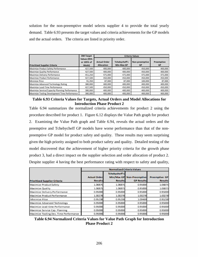
206
solution for the non-preemptive model selects supplier 4 to provide the total yearly
demand. Table 6.93 presents the target values and criteria achievements for the GP models
and the actual orders. The criteria are listed in priority order.
Table 6.94 summarizes the normalized criteria achievements for product 2 using the
procedure described for product 1. Figure 6.12 displays the Value Path graph for product
2. Examining the Value Path graph and Table 6.94, reveals the actual orders and the
preemptive and Tchebycheff GP models have worse performance than that of the non-
preemptive GP model for product safety and quality. These results may seem surprising
given the high priority assigned to both product safety and quality. Detailed testing of the
model discovered that the achievement of higher priority criteria for the growth phase
product 3, had a direct impact on the supplier selection and order allocation of product 2.
Despite supplier 4 having the best performance rating with respect to safety and quality,
Actual Order
Allocation
Tchebycheff's
Min-Max GP
Non-preemptive
GP
Preemptive
GP
Maximize Product Safety Performance 427,500 400,000 400,000 450,000 400,000
Maximize Quality Performance 427,500 400,000 400,000 450,000 400,000
Maximize Delivery Performance 451,250 475,000 475,000 475,000 475,000
Maximize Product Performance 427,500 450,000 450,000 450,000 450,000
Minimize Price 91,350 87,000 87,000 100,000 87,000
Maximize Advanced Technology Rating 380,000 400,000 400,000 400,000 400,000
Maximize Lead-Time Performance 427,500 450,000 450,000 450,000 450,000
Maximize Service/Capacity Planning Performance 380,000 400,000 400,000 400,000 400,000
Maximize Tooling Development Time Performance 380,000 400,000 400,000 400,000 400,000
Prioritized Supplier Criteria
DM Target
Values (95%
or 105% of
Ideals)
Criteria Values
Table 6.93 Criteria Values for Targets, Actual Orders and Model Allocations for
Introduction Phase Product 2
Table 6.94 Normalized Criteria Values for Value Path Graph for Introduction
Phase Product 2

207
supplier 3 was selected. Supplier 4 was chosen to supply 1.6 million units of product 3,
which consumed the entire capacity of supplier 4 with respect to its business volume level.
This business volume constraint combined with the best performance with respect to
quality and safety required the selection of supplier 4 for product 3. Achieving these higher
criteria was again done at the detriment of the lower priority criteria. This real-world
example clearly demonstrates the principles of preemptive goal programming. The non-
preemptive GP model results are equal to or better than the actual orders and those of the
preemptive and Tchebycheff GP models in all criteria except price, which misses by 9.5%.
Figure 6.13 presents a copy of the PowerPoint slide, used in the DM review, which
compares the criteria values achieved by the GP models and the actual orders using the
Value Path graph.
Figure 6.12 Value Path Graph: Comparison of Actual Orders and Model Results for
Introduction Phase Product 2

208
Managerial Feedback
The discussion related to Figure 6.13 focused on the ability to identify opportunities for
supplier performance improvement in order to improve overall performance using the
Value Path graph. Supplier 3’s performance with respect to product safety and quality was
rated at 8 versus supplier 4’s rating of 9 in both of these important criteria. The DM
commented that this situation presented an opportunity for supplier development related to
safety and quality performance. This opportunity could include visits, supplier coaching
and compliance audits by the company’s quality assurance team in order to mitigate any
possible risk from choosing supplier 3, with the intent of improving supplier 3’s safety and
quality performance. The company would then benefit from improved performance from
supplier 3 and be able to take advantage of the price advantage provided by supplier 3 for
product 2.
Figure 6.13 DM Review Actual Orders and GP Model Allocations and Value Path
Graph for Introduction Phase Product 2

209
6.6.4 Growth Phase (Product 3)
Table 6.95 displays the procurement plan by the GP models and the actual orders for
product 3, in the growth phase. Suppliers 3 and 5 were chosen to supply the yearly demand
for both the Tchebycheff and non-preemptive GP models. Suppliers 3 and 4 where selected
to supply the yearly demand for the preemptive model. Supplier 5 was chosen to supply
all of the yearly demand for the actual orders. A constraint limiting the maximum number
of suppliers for the growth phase to two allows splitting the demand between the two
suppliers. Table 6.96 presents the target values and criteria achievements for the actual
orders and the goal programming models. The criteria are listed in priority order.
Actual Order
Allocation
Tchebycheff's
Min-Max GP
Non-preemptive
GP
Preemptive
GP
Maximize Quality Performance 25,650,000 27,000,000 24,222,005 24,723,996 25,600,000
Maximize Product Safety Performance 25,650,000 27,000,000 24,222,005 24,723,996 25,600,000
Maximize Delivery Performance 27,075,000 28,500,000 28,500,000 28,500,000 28,500,000
Maximize Lead-Time Performance 25,650,000 27,000,000 27,000,000 27,000,000 27,000,000
Maximize Service/Capacity Planning Performance 22,800,000 24,000,000 24,000,000 24,000,000 24,000,000
Maximize Product Performance 25,650,000 27,000,000 27,000,000 27,000,000 27,000,000
Minimize Price 27,342,000 28,950,000 26,255,345 26,742,276 28,152,000
Maximize Tooling Development Time Performance 22,800,000 24,000,000 24,000,000 24,000,000 24,000,000
Prioritized Supplier Criteria
DM Target
Values (95%
or 105% of
Ideals)
Criteria Values
Table 6.95 Procurement Plan by GP Model and Actual Orders for Growth Phase
Product 3
Table 6.96 Criteria Values for Targets, Actual Orders and Model Allocations for
Growth Phase Product 3

210
Table 6.97 summarizes the normalized criteria achievements for the product 3. Figure 6.14
displays the Value Path graph for product 3. Examining the Value Path graph and Table
6.97 reveals that the Tchebycheff, non-preemptive and preemptive GP models have worse
performance than those of the actual orders for both quality and safety missing, by 5.9%,
3.7% and 0.2% respectively for both quality and safety. These performance differences
should not be a surprise given that supplier 4 has the highest performance among the
Figure 6.14 Value Path Graph: Comparison of Actual Orders and Model Results for
Growth Phase Product 3
Table 6.97 Normalized Criteria Values for Value Path Graph for Growth Phase
Product 3

211
potential suppliers for both quality and safety. All the models and the actual orders perform
equally well for the delivery, lead-time, service and capacity planning, product
performance and tooling development time goals. Tchebycheff’s min-max model beats
the price target by 5% followed by the non-preemptive model, which beats the price by
2.2%. The preemptive and actual orders miss the price target by 3.0% and 5.9%
respectively.
Managerial Feedback
The results of the growth phase presented the DM with 4 different results with respect to
quality, safety and price performance. While the actual orders displayed the best
performance with respect to quality and safety, it also had the worst performance with
respect to price. The price difference was substantial and the Value Path graph clearly
presents these tradeoffs. Prior to these results being shared with the DM, the company
chose to stop production of product 3 at supplier 5, moving production to the other
suppliers for reasons including better price, reduced transportation costs, reduced duty
costs and proximity to the company’s warehouse.
6.6.5 Mature Phase (Product 4)
Table 6.98 displays the procurement plan by the GP model and the actual orders for product
4, in the mature phase. Suppliers 6 and 7 were chosen to supply the yearly demand for all
of the GP models with order allocations varying by model. Suppliers 1, 2, 6 and 7 were
chosen for the actual orders. Supplier 2 was not included in the initial supplier listing for
the GP models. The company added this supplier later. This selection of a fourth supplier
to provide a mature phase product relaxed the constraint of selecting a maximum of 3
suppliers. The GP models imposed the constraints setting the minimum number of required
suppliers to two and the maximum number of suppliers to three. These constraints
supported the DM’s objective of creating price competition in order to improve the gross
profit margin for mature phase products.

212
Managerial Feedback
The review with the DM pointed out the addition of a fourth supplier and the addition of
supplier 2 as a supply source for product 4 (see Figure 6.15). The DM noted the addition
of a fourth supplier for mature phase product 4, was due to significant unanticipated
customer demand for similar products. This demand spike created world-wide capacity
issues for this product family. In an effort to meet this unexpected demand, supplier 2 was
added as an additional source for mature phase product 4. This addition of supplier 2 also
required the creation of duplicate tooling, increasing the product cost.
Table 6.98 Procurement Plan by GP Model and Actual Orders for Mature Phase
Product 4

213
Table 6.99 presents the target values and criteria achievements for the actual orders and the
goal programming models. The criteria are listed in the priority order.
Table 6.100 summarizes the normalized criteria achievements for the product 4. Figure
6.16 displays the Value Path graph for product 4. The actual orders and the GP models
perform equally well for the safety, quality and product performance. Examining the Value
Actual Order
Allocation
Tchebycheff's
Min-Max GP
Non-preemptive
GP
Preemptive
GP
Maximize Product Safety Performance 3,230,000,000 3,400,000,000 3,400,000,000 3,400,000,000 3,400,000,000
Maximize Quality Performance 3,068,500,000 3,230,000,000 3,230,000,000 3,230,000,000 3,230,000,000
Maximize Product Performance 3,068,500,000 3,230,000,000 3,230,000,000 3,230,000,000 3,230,000,000
Minimize Price 14,994,000 16,490,000 14,623,763 14,996,970 14,994,000
Maximize Past Performance 2,907,000,000 3,026,000,000 3,060,000,000 3,060,000,000 3,060,000,000
Maximize Delivery Performance 3,036,200,000 3,077,000,000 3,060,000,000 3,060,000,000 3,060,000,000
Maximize Service/Capacity Planning Performance 2,907,000,000 3,026,000,000 3,060,000,000 3,060,000,000 3,060,000,000
Maximize Lead-Time Performance 2,907,000,000 3,026,000,000 3,060,000,000 3,060,000,000 3,060,000,000
Maximize Tooling Development Time Performance 2,777,800,000 2,856,000,000 2,584,752,600 2,659,394,000 2,658,800,000
Prioritized Supplier Criteria
DM Target
Values (95% or
105% of Ideals)
Criteria Values
Figure 6.15 DM Review Actual Orders and GP Model Allocations and Value Path
Graph for Mature Phase Product 4
Table 6.99 Criteria Values for Targets, Actual Orders and Model Allocations for
Mature Phase Product 4

214
Path graph and Table 6.100 reveals that the non-preemptive and preemptive GP models
have worse performance than the Tchebycheff model but still achieve the price target. The
actual orders miss the price target by nearly 10%. Delivery performance is slightly better
than the target value for the actual order and the GP models. Likewise, the performance
for both service and capacity planning and lead-time are better than the target values.
While. the actual model betters the tooling development time target by 2.7%, the non-
preemptive, preemptive and Tchebycheff min-max model miss by 4.5%, 4.5% and 7.5%
respectively.
Figure 6.16 Value Path Graph: Comparison of Actual Orders and Model Results for
Mature Phase Product 4
Actual Order
Results
Tchebycheff's
Min/Max GP
Results
Non-Preemptive
GP Results
Preemptive GP
Results
Maximize Product Safety 0.95000 0.95000 0.95000 0.95000
Maximize Quality 0.95000 0.95000 0.95000 0.95000
Maximize Product Performance 0.95000 0.95000 0.95000 0.95000
Minimize Price 1.09977 0.97531 1.00020 1.00000
Maximize Past Performance 0.96067 0.95000 0.95000 0.95000
Maximize Delivery Performance 0.98674 0.99222 0.99222 0.99222
Maximize Service Cap. Planning 0.96067 0.99222 0.95000 0.95000
Maximize Lead-time Performance 0.96067 0.95000 0.95000 0.95000
Maximize Tooling Dev. Time Performance 0.97262 1.07469 1.04452 1.04476
Prioritized Supplier Criteria
Normalized Criteria Values
Table 6.100 Normalized Criteria Values for Value Path Graph for Mature Phase
Product 4

215
Managerial Feedback
While the Value Path graph shows a substantial opportunity to reduce price by choosing
the supplier order allocations using the GP models, it does not consider overall capacity in
the industry and the need to react to unexpected market opportunities. The company made
the choice to service their customers under stressful market and capacity conditions while
sacrificing some product gross margins via increased price.
6.6.6 Mature Phase (Product 5)
Table 6.101 displays the procurement plan by the actual orders and the GP models for
product 5, in the mature phase. Suppliers 2 and 6 were chosen to supply the yearly demand
for all of the GP models with order allocations varying by model. Suppliers 1 and 2 were
chosen for the actual orders. Several constraints impacted the selection of suppliers. The
mature phase sets the minimum number of required suppliers to two and the maximum
number of suppliers to three. This constraint supports the DM’s objective of creating price
competition in order to improve the gross profit margin for mature phase products. Unlike
product 4, these constraints controlling the number of suppliers was adhered to. Table
6.102 presents the target values and criteria achievements for each of the goal programming
models and the actual orders. The criteria are listed in priority order.
Table 6.101 Procurement Plan by GP Model and Actual Orders for Mature Phase
Product 5

216
Table 6.103 summarizes the normalized criteria achievements for the product 5. Figure
6.17 displays the Value Path graph for product 5. Examining the Value Path graph and
Table 6.103 table reveal that all three GP models and the actual orders perform equally
well on the top three priority goals of safety, quality and product performance. The actual
orders miss the price target by 32.7%, while the Tchebycheff GP model misses the price
target by 7.0%, the non-preemptive model achieves the price target and the preemptive GP
solution is better than the price target by 4.8%. Past performance, delivery, service and
capacity planning and lead-time performance perform equal well for all GP models,
bettering the target values by 5.0%, 0.8%, 5.0% and 5.0% respectively. The actual orders
are slightly worse than the target values for past performance, service and capacity
planning and lead-time missing the target values by 0.6%. Delivery performance for the
actual orders betters the target values by 3.5%. All of the models and the actual orders
miss the tooling development time with the misses ranging from 7.5% to 15.5%.
Actual Order
Results
Tchebycheff's
Min/Max GP
Results
Non-Preemptive
GP Results
Preemptive GP
Results
Maximize Product Safety 0.95000 0.95000 0.95000 0.95000
Maximize Quality 0.95000 0.95000 0.95000 0.95000
Maximize Product Performance 0.95000 0.95000 0.95000 0.95000
Minimize Price 1.32688 1.06980 1.00026 0.95238
Maximize Past Performance 1.00588 0.95000 0.95000 0.95000
Maximize Delivery Performance 0.96541 0.99222 0.99222 0.99222
Maximize Service Cap. Planning 1.00588 0.95000 0.95000 0.95000
Maximize Lead-time Performance 1.00588 0.95000 0.95000 0.95000
Maximize Tooling Dev. Time Performance 1.14000 1.07453 1.12100 1.15541
Prioritized Supplier Criteria
Normalized Criteria Values
Actual Order
Allocation
Tchebycheff's
Min-Max GP
Non-preemptive
GP
Preemptive
GP
Maximize Product Safety Performance 1,045,000,000 1,100,000,000 1,100,000,000 1,100,000,000 1,100,000,000
Maximize Quality Performance 992,750,000 1,045,000,000 1,045,000,000 1,045,000,000 1,045,000,000
Maximize Product Performance 992,750,000 1,045,000,000 1,045,000,000 1,045,000,000 1,045,000,000
Minimize Price 4,435,200 5,885,000 4,744,782 4,436,345 4,224,000
Maximize Past Performance 940,500,000 935,000,000 990,000,000 990,000,000 990,000,000
Maximize Delivery Performance 982,300,000 1,017,500,000 990,000,000 990,000,000 990,000,000
Maximize Service/Capacity Planning Performance 940,500,000 935,000,000 990,000,000 990,000,000 990,000,000
Maximize Lead-Time Performance 940,500,000 935,000,000 990,000,000 990,000,000 990,000,000
Maximize Tooling Development Time Performance 940,500,000 825,000,000 875,268,460 838,981,720 814,000,000
Prioritized Supplier Criteria
DM Target
Values (95% or
105% of Ideals)
Criteria Values
Table 6.102 Criteria Values for Targets, Actual Orders and Model Allocations for
Mature Phase Product 5
Table 6.103 Normalized Criteria Values for Value Path Graph for Mature Phase
Product 5

217
Managerial Feedback
The discussion with the DM, regarding the choice of suppliers 1 and 2, discerned the
supplier selections were heavily influenced by supply chain design issues impacting duty
paid, transportation cost and proximity to a facility providing value added services, which
included adding product 5 as part of a larger end consumer package. Supplier 6’s
geographically location negatively impacted duty and transportation costs. Despite these
negative factors regarding the selection of supplier 6, the DM recognized the significant
opportunity to improve price performance presented by the GP model supplier selections.
The DM remains committed to improving the gross profit margin of mature products and
this is a prime example of that opportunity.
Figure 6.17 Value Path Actual Orders and Model Results Comparison for Mature
Phase Product 5

218
6.6.7 Decline Phase (Product 6)
Table 6.104 displays the procurement plan by the GP models and the actual orders for
product 6, in the decline phase. Tchebycheff’s min- max GP model selects suppliers 4 and
10 to provide 45% and 55% of the yearly demand respectively. The non-preemptive and
preemptive models allocate all of the demand to supplier 10. Supplier 4 was chosen to
supply all the yearly demand for the actual orders. Table 6.105 presents the target values
and criteria achievements for each of the goal programming models and the actual orders.
The goals are listed in priority order.
S4 S10
Tchebycheff's Min/Max 11,198 13,802
Non-preemptive 0 25,000
Preemptive 0 25,000
Actual Orders 25,000 0
Optimal Order Allocations1 to Suppliers
by GP ModelSuppliers
1 Maximum number of suppliers set to two suppliers
GP Model
Actual Order
Allocation
Tchebycheff's
Min-Max GP
Non-preemptive
GP
Preemptive
GP
Maximize Product Safety Performance 237,500 225,000 238,802 250,000 250,000
Maximize Quality Performance 225,625 225,000 231,901 237,500 237,500
Minimize Price 107,100 130,000 114,542 102,000 102,000
Maximize Past Performance 190,000 200,000 200,000 200,000 200,000
Maximize Service/Capacity Planning Performance 190,000 200,000 200,000 200,000 200,000
Maximize Product Performance 225,625 225,000 231,901 237,500 237,500
Maximize Delivery Performance 225,625 237,500 216,797 200,000 200,000
Maximize Lead-Time Performance 213,750 225,000 211,198 200,000 200,000
Maximize Tooling Development Time Performance 213,750 200,000 213,802 225,000 225,000
Prioritized Supplier Criteria
DM Target
Values (95% or
105% of Ideals)
Criteria Values
Table 6.104 Procurement Plan by GP Model and Actual Orders for Decline
Phase Product 6
Table 6.105 Criteria Values for Targets, Actual Orders and Model Allocations for
Decline Phase Product 6

219
Table 6.106 summarizes the normalized criteria achievements for the product 6. Figure
6.18 displays the Value Path graph for product 6. Examining the Value Path graph and
Table 6.106 show that the non-preemptive and preemptive GP models display the best
performances for the top three decline phase priorities of safety, quality and price with the
actual orders performing the worst. The actual orders miss the price target by 21.4%. The
three GP models and the actual orders have equal performance for past performance and
service and capacity planning. While all three GP models perform better than the target
value for product performance, the actual orders are slightly worse than the target value
missing by 0.3%. The actual orders outperform the GP models in both the delivery and
lead-time criteria bettering the target values by 5%. The misses by the GP models for these
criteria range from 1.2% to 12.8%. Finally, the actual orders miss the tooling development
time by 6.9%, while the GP model results are better than the target values.
Table 6.106 Normalized Criteria Values for Value Path Graph for Decline Phase
Product 6

220
Managerial Feedback
Like product 4, the DM noted that the selection of supplier 4, to provide all the yearly
demand of product 6, was also impacted by the unanticipated customer demand for similar
products. This demand spike created world-wide capacity issues for this product family.
Supplier 4 was chosen at a higher unit price due to capacity availability, negatively
impacting the gross profit margin in an effort to fulfill customer demand.
Figure 6.18 Value Path Actual Orders and Model Results Comparison for Decline
Phase Product 6

221
6.6.8 Decline Phase (Product 7)
Table 6.107 displays the
procurement plan by the GP
model and the actual orders for
product 7, in the decline phase.
The order allocation is exactly
the same for all the models and
the actual orders making Value
Path analysis a trivial exercise.
Table 6.108 presents the target
values and criteria achievements
for each of the goal programming
models. The goal achievements
exceed the target values for all goals except delivery performance, which misses the target
by 0.3%.
Table 6.109 summarizes the normalized criteria achievements for the product 7. Since the
order allocations are the same for all the GP models and the actual, all the normalized
values are the same. Figure 6.19 displays the Value Path graph for product 7. Likewise,
all values in the Value Path graph are equal.
Actual Order
Allocation
Tchebycheff's
Min-Max GP
Non-preemptive
GP
Preemptive
GP
Maximize Product Safety Performance 142,500 150,000 150,000 150,000 150,000
Maximize Quality Performance 135,375 142,500 142,500 142,500 142,500
Minimize Price 17,640 16,800 16,800 16,800 16,800
Maximize Past Performance 128,250 135,000 135,000 135,000 135,000
Maximize Service/Capacity Planning Performance 128,250 135,000 135,000 135,000 135,000
Maximize Product Performance 135,375 142,500 142,500 142,500 142,500
Maximize Delivery Performance 135,375 135,000 135,000 135,000 135,000
Maximize Lead-Time Performance 128,250 135,000 135,000 135,000 135,000
Maximize Tooling Development Time Performance 128,250 135,000 135,000 135,000 135,000
Prioritized Supplier Criteria
DM Target
Values (95% or
105% of Ideals)
Criteria Values
S1 S7
Tchebycheff's Min/Max 0 15,000
Non-preemptive 0 15,000
Preemptive 0 15,000
Actual Orders 0 15,0001 Maximum number of suppliers set to two suppliers
Optimal Order Allocations1 to Suppliers
by GP ModelSuppliers
GP Model
Table 6.107 Procurement Plan by GP Model and
Actual Orders for Decline Phase Product 7
Table 6.108 Criteria Values for Targets, Actual Orders and Model Allocations for
Decline Phase Product 7
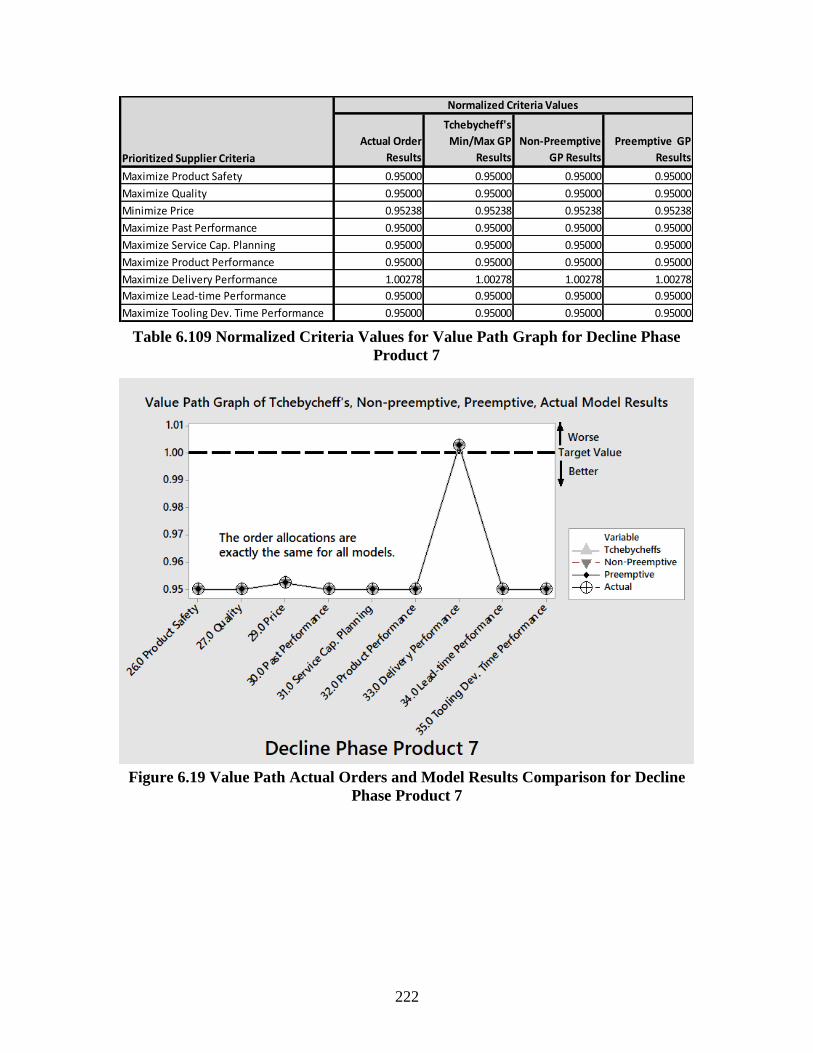
222
Actual Order
Results
Tchebycheff's
Min/Max GP
Results
Non-Preemptive
GP Results
Preemptive GP
Results
Maximize Product Safety 0.95000 0.95000 0.95000 0.95000
Maximize Quality 0.95000 0.95000 0.95000 0.95000
Minimize Price 0.95238 0.95238 0.95238 0.95238
Maximize Past Performance 0.95000 0.95000 0.95000 0.95000
Maximize Service Cap. Planning 0.95000 0.95000 0.95000 0.95000
Maximize Product Performance 0.95000 0.95000 0.95000 0.95000
Maximize Delivery Performance 1.00278 1.00278 1.00278 1.00278
Maximize Lead-time Performance 0.95000 0.95000 0.95000 0.95000
Maximize Tooling Dev. Time Performance 0.95000 0.95000 0.95000 0.95000
Prioritized Supplier Criteria
Normalized Criteria Values
Figure 6.19 Value Path Actual Orders and Model Results Comparison for Decline
Phase Product 7
Table 6.109 Normalized Criteria Values for Value Path Graph for Decline Phase
Product 7

223
6.6.9 Impact on Procurement Cost
This section compares the price criteria results between the actual order and the GP models.
It should be remembered that the preemptive and non-preemptive GP models are based on
the DMs ranking of the criteria. Therefore, the models are simply determining the optimal
order allocations and supplier selections using the decision makers inputs and constraints.
Tchebycheff’s min-max model minimizes the maximum deviation from the target values,
which were set by the DM.
Figure 6.20 displays the procurement cost comparisons for the introduction phase products
1 and 2. The highest total procurement cost for the introduction phase product 1 is the
preemptive GP model at $500M, followed by the actual orders at $460M and the non-
preemptive and Tchebycheff’s min-max model at $450M. This result for the preemptive
model is not surprising given the relatively low priority assigned to the price criterion
during the introduction phase of the product. The price criterion is preceded by product
safety, product quality, delivery performance and product performance supplier selection
criteria and would be subjected to the supplier selections which maximize these criteria.
Figure 6.20 Procurement Cost Comparison of Actual Orders and GP Models for
Introduction Phase Products 1 and 2

224
The best price performance for product 1 belongs to the non-preemptive and Tchebycheff
min-max GP models. The actual orders price performance misses these models by $10,000
or 2.2%.
The introduction phase product 2 has a tie for the best price performance at $87M, which
was achieved by the actual orders, preemptive and Tchebycheff’s min-max GP models.
The non-preemptive model has the worst price performance, which misses the best results
by $13,000 or 14.9%.
Figure 6.21 displays the procurement cost comparisons for the growth phase product 3 and
the mature phase products 4 and 5. The actual procurement cost for growth phase product
3 is the highest at $28.95MM, followed by the preemptive model at $28.152MM, the non-
preemptive model at $26.742MM and finally Tchebycheff’s min-max model at
$26.255MM. The preemptive model has the second highest overall procurement cost
which is not unexpected, given the relatively low priority assigned to the price criterion
during the growth phase of the product. Price is prioritized seventh out of 8 criteria for
Figure 6.21 Procurement Cost Comparison of Actual Orders and GP Models for
Growth Phase Product 3 and Mature Phase Products 4 and 5

225
product 3. The maximum savings opportunity, comparing the actual orders to the
Tchebycheff min-max model results is $2.695MM or a 9.3%.
It should be pointed out that prior to these results being shared with the DM, the company
chose to stop production of product 3 at supplier 5, moving production to other suppliers.
The reasons for this move included better price, reduced transportation costs, reduced duty
costs and proximity to the company’s warehouse. This GP model results clearly support
the company’s decision to move product 3 from supplier 5 to supplier 3.
The actual procurement cost for mature phase product 4 is the highest at $16.49MM,
followed by the non-preemptive model at $14.997MM, the preemptive model at
$14.994MM and finally Tchebycheff’s min-max model at $14.624MM. The non-
preemptive and preemptive model costs are virtually tied. The preemptive model for the
mature phase performs far better than the growth phase. This is not surprising given that
price is now the fourth highest criteria out of 9 selection criteria and compared to the growth
phase price criteria which is ranked seventh out of 8 criteria. The actual procurement cost
misses the best cost performance of the Tchebycheff min-max model by $1.866MM or
11.3%.
The actual order allocations and supplier selections for product 4, was impacted by
significant unanticipated customer demand for similar products. This demand spike
created world-wide capacity issues for this product family. In an effort to meet this
unexpected demand, supplier 2 was added as an additional source for mature phase product
4. This addition of supplier 2 also required the creation of duplicate tooling, increasing the
product cost. All these efforts were done with the intention of providing the best possible
service levels to company’s customers with the possible sacrifice of product 4’s gross profit
margin.
The actual procurement cost for mature phase product 5 is again the highest at $5.885MM,
followed by Tchebycheff’s min-max model at $4.725MM, the non-preemptive model at
$4.436MM and the preemptive model at $4.224MM. It may seem surprising that the

226
preemptive model had the lowest procurement cost given the cost criterion results for the
previous products. The price criterion is prioritized below safety, quality and product
performance for mature phase products. Suppliers 2 and 6 perform equal to or better than
the other potential suppliers for safety, quality and product performance. They also have
the lowest overall unit pricing and therefore have the best procurement cost performance
of the GP models. The actual procurement cost misses this best cost performance by
$1.661MM or 28.2%.
The selection of suppliers 1 and 2 for product 5’s actual orders were heavily influenced by
the supply chain design issues impacting duty paid, transportation cost and proximity to a
facility providing value added services, which included adding product 5 as part of a larger
end consumer package. Supplier 6’s geographic location increased duty and transportation
costs. Despite these increased costs regarding the selection of supplier 6, the DM
recognized the significant opportunity to improve price performance presented by the GP
model supplier selections. The DM remains committed to improving the gross profit
margin of mature products and the GP models provide that opportunity.
Figure 6.22 displays the procurement cost comparisons for the decline phase products 6
and 7. The actual cost for decline phase product 6 is the highest at $130M, followed by
Tchebycheff’s min-max model at $114M, the non-preemptive and the preemptive models
at $102M. Once again, the preemptive model has the lowest procurement price criteria
performance along with the non-preemptive model. Supplier 10 has the best performance
for safety, quality and price, necessitating the choice of supplier 10 to supply all of the
demand for product 6. The actual orders were allocated to supplier 4 at a substantial price
increase as compared to supplier 10. This example further emphasizes the effectiveness of
the GP models to provide optimal solutions using the DM’s criteria ranking and weights.

227
Decline phase product 7’s procurement cost results are the same for the actual orders and
the GP models. Supplier 7 is selected to supply all the demand for the actual orders and
all the GP models and they all have the same procurement cost of $17M.
Figure 6.23 presents a copy of the PowerPoint slide, included in the review with the DM
illustrating the cost comparisons between the actual order allocations and the goal
programming models. The best total price improvement, compared to the actual order
allocations, is the Tchebycheff min-max model with a $5.727MM savings and a 11.0%
price improvement. The next highest price improvement versus the actual orders is the
non-preemptive model, with a $5.174MM savings and a 9.9% price improvement. Finally,
the preemptive model saves $3.943MM with a corresponding 7.6% price performance
improvement. While there were a number of “real world” circumstances which impacted
the actual order allocations, such as unanticipated demand, transportation and supply chain
design issues, these potential savings projections reinforce the effectiveness of the GP
models in generating significant savings in supplier procurement costs.
Figure 6.22 Procurement Cost Comparison of Actual Orders and GP Models for
Decline Phase Products 6 and 7

228
6.7 Chapter Summary
The case study results illustrate the effectiveness of the Goal Programming (GP) models in
selecting suppliers and allocating orders for products across the product life cycle. The
focal company is a U.S. based consumer products company which utilizes a diverse global
supply chain to design, manufacture and deliver products to traditional brick and mortar
retailers, on-line retailers and distributors. Three key executive decision makers were
employed to identify and rank the key sourcing criteria attributes for products representing
the introduction, growth, mature and decline phases of the product life cycle. Seven
products were selected representing three of four top selling product families. The
suppliers included in this case study have already been pre-screened and short-listed by the
company.
Figure 6.23 DM Review of the Price Achievements for Actual Order and GP Models

229
The case study also provides a unique opportunity to view the supplier attributes, such as
product safety, product performance, service and capacity planning, which are driving the
global supplier selection process throughout the product life cycle. Many of the
performance criteria are beyond the traditional metrics of delivery, quality, cost and lead-
time. In addition to these selection criteria, there were business volume constraints
included in the GP models. These business volume constraints were based on several
factors including whether the suppliers were new or existing suppliers. Total purchases
from new suppliers were limited to 10% or 20% of their total sales revenue, while existing
suppliers were limited to 30% or 40% of their total sales revenue. These limits were set
by the company in an effort to minimize supplier performance risk. Additionally, there
were constraints on the minimum and maximum number of suppliers by product life cycle
phase. New products, during their introduction phase, were limited to just one supplier.
Mature products were required to have a minimum of two suppliers and a maximum of
three suppliers in order to insure there was price competition among the suppliers, with the
objective of improving the gross profit margin of mature products.
The preemptive and non-preemptive GP models utilized the DM’s ranking results to
determine the optimal supplier selections and order allocations that come as close as
possible to the targets set by the DMs for the different supplier criteria. The Tchebycheff
min-max model, which does not use any decision maker’s inputs simply minimized the
maximum deviation from the target values. The results were shared with the DMs using
the Value Path approach, which graphically displays the results and allows decision makers
to choose the best solution. During the review of the product 1 results (introduction phase),
using the Value Path graphs, the decision makers commented that the tradeoff of 5.6% in
delivery performance improvement may be considered in order to improve the other
supplier criteria. This is an example of the power of the Value Path method in comparing
alternative solutions and performance tradeoffs. The DMs also considered relaxing some
of the business constraints, such as total business volume for supplier 4. Relaxing this
business volume constraint could positively impact the safety and quality performance for
both the introduction phase (product 2) and growth phase (product 3). Additional model
testing could be easily accomplished providing a new set of optimal solutions to the DMs.

230
This is another benefit of utilizing an integrated supplier selection model to support
sourcing decisions. While the results from no single GP model generated optimal results
for all products and across the product life cycle, the Value Path results presented the DMs
with performance tradeoffs that could be used in selecting the optimal sourcing strategies.
In order to test the effectiveness of the model, the actual orders were compared to the GP
model results. The actual supplier orders for the case study items, for the same time period,
were obtained for this managerial evaluation. Several key differences existed with regards
to the constraints utilized to create the GP models and the actual order allocations. The
company relaxed some constraints during the actual order allocations. Limits on the
maximum number of suppliers by product life cycle phase were increased. Suppliers not
included in the initial supplier listing were utilized in the actual order allocations. These
business rules or constraints were relaxed for a number of reasons, including supplier chain
design issues impacting duty paid, transportation cost and geographic location. In addition,
unanticipated demands created world-wide capacity issues for several product families
included in the case study. Suppliers were added to meet this increased demand at higher
procurement costs.
Even though the GP models used more restrictive constraints, the actual orders in general
performed poorly, when compared to the GP model results! One of the significant
conclusions was that the model results provided a substantial savings in procurement costs,
while maintaining quality, delivery and safety criteria performance. The potential total
savings in procurement costs, from utilizing the GP models, was $5.727MM for the
Tchebycheff min-max model (11% reduction) and $5.174MM savings for the non-
preemptive and preemptive models (9.9% reduction). Imagine the potential savings, if this
integrated supplier selection model is widely implemented to support procurement
strategies and supplier selection decisions across all the company products!
In addition to identifying the substantial cost advantage, another benefit of comparing the
actual results to the GP model results is the ability to identify opportunities for supplier
development. During the review of the Value Path results, the decision maker identified

231
several opportunities for supplier development to improve the supplier performance in
product safety and quality, in order to mitigate potential risk, and gain better price
performance. Visualizing these tradeoffs using the Value Path graphs, identified potential
tradeoffs between the GP models and the actual results. The DM commented that the actual
orders could be blended with the model results to generate better sourcing strategies. This
statement reveals another significant benefit of utilizing this integrated decision-making
model, which allows “what if” scenarios to be easily tried, including changing goal priority
weights, priorities and relaxing business constraints providing the DMs with alternative
solutions and better results. While there may not be a single solution which meets all the
DM’s objectives, a blended solution generated through a number of problem-solving
iterations may provide a best answer to the product life cycle sourcing problem.

232
7. Conclusion and Future Research This final chapter will summarize the dissertation’s contributions to modeling the supplier
selection problem, its practical significance and potential future research.
7.1 Summary of Model Contributions to Supplier Selection
This dissertation develops an integrated multiple criteria supplier selection model with
product life cycle considerations. A summary of modeling contributions of this dissertation
are:
▪ An approach to analyze supplier performance using ordinal logistic regression to
test relationships between key supplier attributes and quality and delivery
performance. An empirical model was created using supplier attributes and
performance data from an industrial equipment manufacturer. A number of
hypotheses were tested on the relationship between attributes such as quality
certifications, such as ISO 9001:2015, and quality and delivery performance. The
results and methodology provide a framework which can be used to develop
constraints to be included in an integrated supplier selection model, with the intent
of improving supplier performance. This methodology could also be used to short-
list suppliers in a multi-step supplier selection process (Chapter 3).
▪ Supplier selection is a multiple criteria optimization problem with conflicting
criteria, such as quality, delivery, service, product safety and others. Several
multiple criteria sourcing models exist in the literature. Very rarely they have
considered the fact that the relative importance of the supplier attributes depends
on the product life cycle phase. For example, during the Introduction phase,
companies may work with a single supplier emphasizing product safety, quality
and delivery. Revenue targets are more important than gross profit margins.
However, during the Growth phase, multiple suppliers may be used to meet surging
demand and to introduce price competition among the suppliers. In the Mature
phase, controlling procurement cost becomes important in order to boost the

233
product gross profit margin. In addition, many suppliers can deliver materials
needed for multiple products under various stages of the product life cycle phase.
Companies may also limit the business volume to new and existing suppliers. All
these factors are integrated into a general model in this thesis. A multiple criteria,
multiple products, supplier selection model that explicitly considers the product life
cycle phases of the products is developed. The goal programming approach is used
to solve the multiple criteria problem. An example was used to illustrate the
different programming solution approaches, including preemptive GP, non-
preemptive GP, Tchebycheff’s min-max GP and fuzzy GP. This general model
included products from the introduction, growth, maturity and decline phases of the
product life cycle. Also included in the model were parameters, based on the
results of the empirical study, including maximum business level, minimum
financial condition and minimum required quality technical capability. Multiple
objectives for the model included the minimization of cost, lead-time, quality
defects and late deliveries. Constraints specifying the maximum and minimum
number of suppliers by product life cycle phase were included in the model. The
Value Path method was utilized to provide visual tradeoffs of the multiple criteria
for product across the product life cycle (Chapter 4).
▪ The general supplier selection model from Chapter 4 was applied to a real-world
problem. This case study is focused on a U.S. based consumer products company
which utilizes a diverse global supply chain to design, manufacture and deliver
products to traditional brick and mortar retailers, on-line retailers and distributors.
Three key executive decision makers (Chief Operating Officer,
VP for Procurement and Global Sourcing Manager) were employed to identify and
rank the key sourcing criteria attributes for products representing the introduction,
growth, mature and decline phases of the product life cycle. Ranking methods
included rating method, Borda count utilizing pairwise comparisons and the
Analytic Hierarchy Process. The DMs shared their feedback on the cognitive
burden for each of the ranking methods. Ranking results indicate the DM’s
priorities change based on the product life cycle phase. The ranking results were

234
reviewed with the DMs and the feedback from this review was noted. The
contributions of this first part of the case study include providing insights relating
supplier attributes, to the DMs’ preferences which change throughout the product
life cycle and feedback regarding the cognitive burden required by the ranking
methods (Chapter 5).
▪ The supplier selection criteria weights and rankings, determined in Chapter 5, were
utilized in the preemptive and non-preemptive goal programming models to
determine final supplier selections and optimal order allocations for the case study.
In addition, Tchebycheff’s min-max and fuzzy goal programming methods were
also employed to determine final supplier selections and optimal order allocations.
The Value Path approach was utilized to compare the results from the preemptive,
non-preemptive and Tchebycheff GP models. The results were reviewed with the
DMs and the feedback from this review was discussed. In order to assess the
effectiveness of the model results, a comparison of the GP model results to actual
order allocations that were used by the company was completed. The GP model
results exceeded the actual order allocation criteria performance for many of the
products throughout the product life cycle phases. The results were presented to
the Chief Operating Officer (COO) using the Value Path approach. The COO
provided extensive feedback and had observations on how the model results could
be blended to examine alternate solutions. Also, he identified opportunities for the
company to improve supplier performance in an effort to minimize supplier
performance risk (Chapter 6).
7.2 Summary of Practical Significance
The methodology in Chapter 3 provides a template which can be customized for a company
linking key supplier attributes and performance measures. The ordinal logistic regression
is a general model which can be utilized to determine significant factors or supplier
attributes impacting performance. While the empirical model tests supplier quality and
delivery performance to key supplier attributes, a company can choose performance
metrics critical to their organization. For example, product safety would be of utmost

235
importance in the children’s toy industry and therefore be included in the modeling process.
Once the relationships are statistically confirmed and the model results are verified, the
predictive model results can be included in the creation of supplier selection models via
the addition of specific constraints. These results could also be utilized in a multi-step
supplier selection process providing guidance to create a short-list of suppliers. Companies
using this approach could gain a competitive edge through the use of this predictive model
with the intent of reducing the risk from poor supplier performance.
The general model presented in Chapter 4 offers a methodology to integrate the results of
a predictive supplier performance model from Chapter 3 into an integrated supplier
selection model with product life cycle considerations. The results of the preemptive, non-
preemptive and Tchebycheff min-max GP models provide alternative optimal solutions,
which can be used by DM to evaluate the results and tradeoffs for conflicting multiple
criteria across the product life cycle. The fuzzy GP results provide the DM with a result
which minimizes the maximum deviation from the ideal values, without any input from the
DM. The fuzzy model results inform the DM of the minimization of the “worst case”
optimal scenario. The Value Path approach provides a visual representation of the four
objectives (cost, lead-time, quality and delivery), for each of the products in their respective
phase of the product life cycle. While there is no single GP model that provides the best
overall solution for all product life cycle phases, the Value Path method provides the DM
with alternative solutions to choose from. Another significant benefit of using the GP
models and Value Path method is the flexibility to respond to the decision maker requests,
such as changing the target values, priority order or weights, by quickly providing
alternative solutions. Once the models have been developed and tested, it is relatively easy
to respond to these requests, providing a powerful decision support tool to the DM.
The real-world case study presented in Chapters 5 and 6, provides a unique opportunity to
view the supplier attributes, such as product safety, product performance, service and
capacity planning, which are driving the global supplier selection process. Many of the
performance criteria are beyond the traditional metrics of delivery, quality, cost and lead-
time. In addition to these selection criteria, there were business volume constraints applied

236
to the suppliers. This business volume was based on several factors including whether the
suppliers were new or existing suppliers. Total purchases from new suppliers were limited
to 10% or 20% of their total sales revenue, while existing suppliers were limited to 30% or
40% of their total sales revenue. These limits were created in an effort to minimize supplier
performance risk to the company. Additionally, there were constraints on the minimum
and maximum number of suppliers by product life cycle phase. Mature products were
required to have at minimum of two suppliers and a maximum of three suppliers in order
to insure there was price competition among the suppliers, with the objective of improving
the gross profit margins of high volume mature products. This was a stated goal of the
senior decision makers. The ranking results also varied by decision maker, the Chief
Operating Officer and the VP of Procurement were very consistent in their rankings results
and took a more strategic view of the selection criteria and product life cycle phases, while
the Global Sourcing Manager’s ranking results reflected a more tactical view. The results
provided an unfiltered view of the executive decision makers’ criteria selection and other
methods used to achieve improved supplier and supply chain results, while minimizing
supplier risk.
The case study results illustrate the effectiveness of the goal programming models in
selecting suppliers and allocating orders for products across the product life cycle. The
decision makers quickly understood the significance of the Value Path results and were
focused on choosing the best overall sourcing strategy based on their supplier criteria
rankings and weights. The DMs also considered relaxing some of their earlier business
constraints, such as total business volume, given the impact of this constraint on the optimal
solution. Additional model testing with modified constraints could be easily accomplished
to provide a new set of solutions to the DMs. This is another practical benefit of utilizing
an integrated supplier selection model to support sourcing decisions.
In order to test the effectiveness of the model, the actual orders were compared to the GP
model results. The actual orders in general performed poorly, when compared to the GP
model results. One of the significant conclusions was that the model results provided
substantial savings in procurement costs, while maintaining quality, delivery and safety

237
criteria performance. A number of factors, such as unanticipated demand, supplier capacity
constraints and supply chain designs, impacted the actual order allocations. One of the
benefits of comparing the actual results to the GP model results includes the ability to
identify opportunities for long term supplier development. During the review of the Value
Path results, comparing the GP models to the actual order allocations, the decision maker
identified opportunities for supplier development to improve supplier performance in
product safety and quality, in order to mitigate potential risk, while gaining better price
performance. The DM clearly understood the tradeoffs in supplier criteria between the GP
models and the actual results using the Value Path results. He observed that the actual
orders could be blended with the model results with the intent of generating better sourcing
strategies. This statement truly reveals the strength of this integrated decision-making
model, which allows “what if” scenarios to be easily tried, including changing goal
priorities and relaxing business constraints and provides the DMs with alternative sourcing
strategies to consider.
7.3 Future Research Opportunities
While this research provides an integrated global supplier selection model with product life
cycle considerations, a number of alternative methods and extensions of the model would
further extend the theoretical and practical applications. Other multiple criteria approaches
that do not use goal programming could be tested and results can be compared.
Another extension of this research would be to consider interactive methods. The case
study (Chapter 5) provides complete information from the DMs with regards to preferences
which were generated using the Analytic Hierarchy Process. Additionally, specific
constraints such as the percentage of total revenue allowed by supplier, minimum and
maximum number of suppliers by product life cycle phase, etc. making this case study a
seemingly good fit for interactive methods.
The integrated model can be extended to a multiple period supplier selection problem in
order to determine the actual supplier orders for each time period over a planning horizon.
Dynamic programming could be used to solve this problem. The stages of the problem

238
could represent transitions to the next stage as products move through the product life cycle
phases, with demand, supplier selection criteria and constraints changing. Initially, a
deterministic dynamic program could be formulated and solved. Next, demand variation
could be included as random variables transforming the problem to a stochastic dynamic
program.
The addition of multiple periods to the preemptive, non-preemptive, Tchebycheff’s min-
max and fuzzy goal programs would be a beneficial extension of the general model.
Products could transition through the product life cycle phases with supply sources,
constraints, demand and goal objectives via the addition of multiple periods. As noted
previously, this addition of multiple periods might also be a great fit for the dynamic
programming methodology.

239
References
Agresti, Alan (1984), Analysis of Ordinal Categorical Data, John Wiley and Sons, New
York, NY.
Agresti, Alan (2002), Categorical Data Analysis, 2nd Edition, John Wiley & Sons, New
York, NY.
Bartholomew, Doug (2006), Supply Chains at Risk, Industry Week, 255(10): 54-60.
Bender, Paul S.; Brown, Richard W.; Isaac, Michael H. and Shapiro, Jeremy F. (1985),
Improving Purchasing Productivity at IBM with a Normative Decision Support System,
Interfaces,15(3): 106-115.
Benton, W.C. and Krajewski, Lee (1990), Vendor Performance and Alternative
Manufacturing Environments, Decision Sciences, 21(2): 403-415.
Bhutta, Khurrum S. and Huq, Faizul (2002), Supplier Selection Problem: A Comparison
of the Total Cost of Ownership and Analytic Hierarchy Process Approaches, Supply
Chain Management, 7(3): 126-135.
Bianco, Anthony; Zellner, Wendy; Brady, Diane; France, Mike; Lowry, Tom; Byrnes,
Nanette; Zegel, Susan; Arndt, Michael; Berner, Robert and Palmer, Ann Therese (2003),
Is Wal-Mart Too Powerful?, Business Week, Iss. 3852, New York, NY.
Bowersox, Donald J.; Closs, David J. and Cooper, M. Bixby (2002), Supply Chain
Logistics Management, McGraw-Hill, New York, NY.
Breyfogle III, Forest W. (1999), Implementing Six Sigma, John Wiley & Sons, New
York, NY.
Buffa, Frank P. and Jackson, Wade M. (1983), A Goal Programming Model for Purchase
Planning, Journal of Purchasing and Materials Management, 19(3): 27-34
Burt, David N., Dobler, Donald W. and Starling, Stephen L. (2003), World Class Supply
ManagementSM The Key to Supply Chain Management, 7th Edition, New York, NY,
McGraw-Hill.
Carbone, James (2003), Where are the parts?, Purchasing, 132(19): 44-47.
Carr, Amelia S. and Smeltzer, Larry R. (1999), The Relationship Among Purchasing
Benchmarking, Strategic Purchasing, Firm Performance, and Firm Size, The Journal of
Supply Chain Management, 35(4): 51-60.
240
Carter, Phillip L.; Carter, Joseph R.; Monczka, Robert M.; Slaight, Thomas H. and Swan,
Andrew J. (1998), The Future of Purchasing and Supply A Five- and Ten-Year Forecast,
Center for Advanced Purchasing Studies, Tempe, Arizona.
Chapman, Paul; Christopher, Martin; Jüttner, Uta; Peck, Helen and Wilding, Richard
(2002), Identification and Managing Supply Chain Vulnerability, Logistics and
Transportation Focus, 4(4): 59-64.
Choi, Thomas Y., and Hartley, Janet L. (1996), An Exploration of Supplier Selection
Practices Across the Supply Chain, Journal of Operations Management, 14(4): 333-343.
Chopra, Sunil and Sodhi, ManMohan, S. (2004), Managing Risk to Avoid Supply-Chain
Breakdown, Sloan Management Review, 46(1): 53-61.
Chopra, Sunil; Reinhardt, Gilles and Mohan, Usha (2007), The Importance of Decoupling
Recurrent and Disruption Risks in a Supply Chain, Naval Research Logistics, 54(5): 544-
555.
Cohen, Jacob; Cohen, Patricia; West, Stephen G.; Aiken, Leona S. (2003), Applied
Multiple Regression/Correlation Analysis for the Behavioral Sciences, 3rd Edition,
Lawrence Erlbaum Associates Publishers, Mahwah, NJ.
Cox, Andrew (2001A), Understanding Buyer and Supplier Power: A Framework for
Procurement and Supply Competence, Journal of Supply Chain Management, 37(2): 8-
15.
Cox, Andrew (2001B), Managing with Power: Strategies for Improving Value
Appropriation from Supply Relationships, Journal of Supply Chain Management, 37(2);
42-47.
Coyle, John J.; Bardi, Edward J. and Novack, Robert A. (2000), Transportation, 5th
Edition, South-Western College Publishing, Cincinnati, OH.
de Boer, Luitzen; Labro, Eva and Morlacchi, Pierangela (2001), A review of methods
supporting supplier selection, European Journal of Purchasing and Supply Management,
7: 75-89.
Dickson, Gary W. (1966), An Analysis of Vendor Selection Systems and Decisions,
Journal of Purchasing, 2(1): 5- 17.
Dow Jones Factiva Financial Profile Database Search (2018), Web address:
https://www.dowjones.com/products/factiva/.
Dun and Bradstreet Supply Management Solutions Website (2018), Web address:
www.dnb.com/solutions/supply-chain-management.html.

241
Dun and Bradstreet Business Information Report (BIR) documentation (2018), Web
address: https://businesscredit.dnb.com/product/business-information-report/.
Dyer, Jeffrey (1996), How Chrysler Created an American Keiretsu, Harvard Business
Review, 74(4): 42-56.
Ebrahimpour, M.; Withers, B.E. and Hikmet, N. (1997), Experiences of US- and foreign-
owned firms: a new perspective on ISO 9000 implementation, International Journal of
Production Research, 35(2): 569-576.
Ellram, Lisa M. (1990), The Supplier Selection Decision in Strategic Partnerships,
Journal of Purchasing and Materials Management, 26(4): 8-14.
Ellram, Lisa and Billington, Corey (2001), Purchasing Leverage Considerations in the
Outsourcing Decision, European Journal of Purchasing & Supply Management, 7(1): 15-
27.
Emerson, Richard M. 1962, Power-Dependence Relations, American Sociological
Review, 27(1): 31-41.
Evans, James R. and Lindsay, William M. (2002), The Management and Control of
Quality, 5th edition, South-Western, Cincinnati, Ohio..
Fandel, G. and Stammen, M. (2004), A General Model for Strategic Supply Chain
Management with Emphasis on Product Life Cycles including Development and
Recycling, International Journal of Production Economics, 89(3): 293-308.
Feng, Chang-Xue (Jack); Wang, Jin and Wang, Jin-Song (2001), An Optimization Model
for Concurrent Selection of Tolerances and Suppliers, Computers and Industrial
Engineering, 40(1): 15-33.
Fisher, Marshall L. (1997) What is the right supply chain for your product?, Harvard
Business Review, 75 (2): 105-116.
Fortune 500 and 1000 Company Listings (2003), Fortune, 147(7): F-1 to F-71.
Fortune Industrial and Farm Equipment (35 Companies) Listing (2003), Fortune, 147(7):
F-54 to F-55.
Fortune Wholesalers: Diversified (15 Companies) Listing (2003), Fortune, 147(7): F-66.
French, Jr. John R. P. and Raven, Bertram (1959), The Bases of Social Power, Studies in
Social Power, Dorwin Cartwright- editor, University of Michigan Press, Ann Arbor, MI.:
50-167.
Fraering, Martin and Prasad, Sameer (1999), International Sourcing and Logistics: an
Integrated Model, Logistics Information Management, 12(6): 451-459.

242
Ghodsypour, S.H. and O'Brien, C. (1998), A Decision Support System for Supplier
Selection using an Integrated Analytic Hierarchy Process and Linear Programming,
International Journal of Production Economics, 56-57: 199-212.
Ghodsypour, S.H. and O’Brien, C.O. (2001), The Total Cost of Logistics in Supplier
Selection, under Conditions of Multiple Sourcing, Multiple Criteria and Capacity
Constraint, International Journal of Production Economics, 73: 15-27.
Gregory, Robert E. (1986), Source Selection: A Matrix Approach, Journal of Purchasing
and Materials Management, 22(2): 24-29.
Gosman, Martin L. and Kelly, Trish (2002), Big Customers and Their Suppliers: A Case
Examining Changes in Business Relationships and Their Financial Effects, Issues in
Accounting Education, 17(1):41-56.
Handfield, Robert B. and Pannesi, Ronald T. (1994), Managing Component Life Cycles
in Dynamic Technological Environments, International Journal of Purchasing and
Materials Management, 30(2): 20- 27.
Handfield, Robert B., Krause, Daniel R., Scannell, Thomas V. and Monczka, Robert M.,
(2000) Avoid the Pitfalls in Supplier Development, Sloan Management Review,
4192):37-49.
Hendrick, Thomas and Ellram, Lisa (1993), Strategic Supplier Partnering: An
International Study, Center for Advanced Purchasing Studies, Tempe, Arizona.
Hendricks, Kevin B. and Singhal, Vinod R. (2003)., The effect of supply chain glitches on
shareholder wealth, Journal of Operations Management, 21(5): 501-522.
Hendricks, Kevin B. and Singhal, Vindod R. (2005), Association Between Supply Chain
Glitches and Operating Performance, Management Science, 51(5): 695-711.
Heizer, Jay and Render, Barry (2004), Operations Management, 7th Edition, Pearson
Education (Prentice Hall), Upper Saddle River, NJ.
Ittner, Christopher D.; Larcker, David F.; Nagar, Venkatesh and Rajan, Madhav V.
(1999), Supplier Selection, Monitoring Practices and Firm Performance, Journal of
Accounting and Public Policy, 18(3): 253-281.
Jorgensen, Barbara (2005), A New Spin on an Old Problem, Electronic Business, 35(12):
26-27.
Karimi, Hossein and Rezaeinia, Alireza (2014), Supplier selection using revised multi-
segment goal programming model, International Journal of Advanced Manufacturing
Technology, 70, 1227-1234.

243
Kleinbaum, David G.; Kupper, Lawrence L., ; Muller, Keith E. and Nizam, Azhar (1998),
Applied Regression Analysis and Other Multivariable Methods, 3rd Edition, Duxbury
Press, Pacific Grove, CA., www.duxbury.com.
Kraljic, Peter, Purchasing Must Become Supply Management, Harvard Business Review,
61(5): 109-117.
Kotler, Philip (2003), Marketing Management, 11th Edition, Prentice Hall, Upper Saddle
River, NJ.
Krause, Daniel and Scannell, Thomas V. (2002), Supplier Development Practices:
Product- and Service-Based Industry Comparisons, The Journal of Supply Chain
Management, 38(2): 13-21.
Krause, Daniel R., Supplier Development: Current Practices and Outcomes, International
Journal of Purchasing and Materials Management, 33(2):12-19.
Kumar, Manoj; Vrat, Prem and Shankar, R. (2004), A Fuzzy Goal Programming
Approach for Vendor Selection Problem in a Supply Chain, Computers & Industrial
Engineering, 46: 69-85.
Laios, Lambros and Moschuris, Socrates (1999), An Empirical Investigation of
Outsourcing Decisions, The Journal of Supply Chain Management, 35(1): 33-41.
Landry, John T. (1998), Supply Chain Management: The Case for Alliances, Harvard
Business Review, 76(6):24-25.
Lee, Eon-Kyung; Ha, Sungdo and Kim, Sheung-Kown (2001), Supplier Selection and
Management System Considering Relationships in Supply Chain Management, IEEE
Transactions on Engineering Management, 48(3): 307-317.
Li, C.C.; Fun, Y.P.; and Hung, J.S. (1997), A New Measure for Supplier Performance
Evaluation, IIE Transactions, 29(9): 753-758.
Li, Zhi; Wong W.K.; and Kwong, C.K. (2013), An Integrated Model of Material Supplier
Selection and Order Allocation Using Fuzzy Extended AHP and Multiobjective
Programming, Mathematical Problems in Engineering, 1-14;
Liu, Jian; Ding, Fong-Yuen and Lall, Vinod (2000), Using Date Envelopment Analysis to
Compare Suppliers for Supplier Selection and Performance Improvement, Supply Chain
Management: An International Journal, 5(3): 143-150.
Maloni, Michael and Benton, W.C., Power Influences in the Supply Chain, Journal of
Business Logistics, 21(1): 49-73.

244
Masud, Abu S. M. and Ravindran, A. Ravi (2008). Chapter 5: Multiple Criteria Decision
Making, Operations Research and Management Science Handbook, A. Ravi Ravindran
(Editor), CRC Press, Taylor & Francis Group, Boca Raton, FL.
Mendoza, A.; Ravindran, A. Ravi and Santiago, E. (2008), A Three-Phase Multicriteria
Method to the Supplier Selection Process, International Journal of Industrial Engineering,
15(2): 195-220.
Monczka, Robert; Trent, Robert and Handfield, Robert (2002), Purchasing and Supply
Chain Management 2nd Edition, South-Western, Cincinnati, Ohio.
Muralidharan, C.; Anantharaman, N. and Deshmukh S. G. (2002), A Multi-Criteria
Group Decisionmaking Model for Supplier Rating, Journal of Supply Chain
Management, 38(4): 22-33.
Narasimhan, Ram; Talluri, Srinivas and Mendez, David (2001), Supplier Evaluation and
Rationalization via Data Envelopment Analysis: An Empirical Examination, Journal of
Supply Chain Management, 37(3): 28-37.
Narasimhan, Ram; Talluri, Srinivas and Mahapatra, Santosh K. (2006), Multiproduct,
Multicriteria Model for Supplier Selection with Product Life-Cycle Considerations,
Decision Sciences, 37(4):. 557-603.
Narasimhan, Ram and Stoynoff, Linda K. (1986), Optimizing Aggregate Procurement
Allocation Decisions, Journal of Purchasing and Materials Management, 22(1): 23-30.
Novak, Sharon and Eppinger, Steven D. (2001), Sourcing by Design: Product Complexity
and the Supply Chain, Management Science, 47(1): 189-204.
Park, Seungwook and Hartley, Janet L. (2002)., Exploring the Effect of Supplier
Management on Performance in the Korean Automotive Supply Chain, The Journal of
Supply Chain Management, 38(1): 46-53.
Petroni, Alberto and Braglia, Marcello (2000), Vendor Selection Using Principal
Component Analysis, The Journal of Supply Chain Management, 36(2): 63-69.
Porter, Anne Millen (2001), Big Companies struggle to act their size, Purchasing,
130(21): 25-32.
Rao, S. Subba; Ragu-Nathan, T.S. and Solis, Luis E. (1997), Does ISO 9000 have an
effect on quality management practices? An international empirical study, Total Quality
Management, 8(6): 335-346.
Ravindran, A.; Phillips, Don. T and Solberg, James J. (1987), Operations Research
Principles and Practice, 2nd Edition, John Wiley & Sons, New York, NY.

245
Ravindran, A. Ravi and Wadhwa, Vijay (2009). Chapter 4: Multiple Criteria
Optimization Models for Supplier Selection, HANDBOOK OF MILITARY
INDUSTRIAL ENGINEERING, Adedeji Badiru and Marlin Thomas (Editors), CRC
Press, Boca Raton, FL.
Ravindran A. Ravi and Warsing, Jr., Donald P. (2013), Supply Chain Engineering
Models and Applications, CRC Press, Boca Raton, FL.
Rohbe Company Supplier Analysis System Website (2008):
http://www.rohbe.com/prod1.html, 9/7/08.
Saaty, Thomas L. (1980), The Analytic Hierarchy Process, New York, NY, McGraw-
Hill.
Sarkis, Joseph and Talluri, Srinivas (2002), A Model for Strategic Supplier Selection,
Journal of Supply Chain Management, 38(1): 18-28.
Shin, Wan S. and Ravindran, A. (1991), Interactive Multiple Objective Optimization:
Survey I - Continuous Case, Computers & Operations Research, 18 (1): 97-114.
Shirouzu, Norihiko (2000), Ford to Slow Pace of New-Product Launches After Recalls ---
Actions are Intended to Respond to Growing Complaints From Auto Dealers, The Wall
Street Journal, 12/1/2000, B2.
Shirouzu, Norihiko and White, Joseph B. (2002), Three Big Auto Makers Scramble to
Raise Vehicle Quality--- Surveys Find Toyota and Honda Continue to Set the Pace for the
Industry, The Wall Street Journal, 4/1/2002, B4
Simmons, Bret L. and White, Margaret A. (1999), The Relationship Between ISO9000
and Business Performance: Does Registration Really Matter?, Journal of Managerial
Issues, 11(3): 330-343.
Smytka, Daniel L. and Clemens, Michael W. (1993), Total Cost Supplier Selection: A
Case Study, International Journal of Purchasing and Materials Management, 29 (1): 42-
49.
Snyder, Lawrence V. and Shen, Zuo-Jun Max (2006), Managing Disruptions to Supply
Chains, The Bridge- National Academy of Engineering, Winter.
Solomon, Rajeev; Sandborn, Peter A. and Pecht, Michael G. (2000), Electronic Part Life
Cycle Concepts and Obsolescence Forecasting, IEEE Transaction on Components and
Packaging Technologies, 23(4): 707-717.
Stogdill, Ronald C. (1999), Dealing with Obsolete Parts, IEEE Design & Test of
Computers, 16(2): 17-25.

246
Tan, Keah-Choon; Kannan, Vijay R.; Handfield, Robert B. and Ghosh, Soumen (1999),
Supply Chain Management: an Empirical Study of its Impact on Performance,
International Journal of Operations & Production Management, 19(10): 1034-1052.
Tan, Keah Choon (2002), Supply Chain Management: Practices, Concerns, and
Performance Issues, The Journal of Supply Chain Management, 38(1): 42-52.
Tang, Christopher S. (2006A), Perspectives in supply chain risk management,
International Journal of Production Economics, 103, 2006, pp. 451-488.
Tang, Christopher S. (2006B), Robust Strategies for Mitigating Supply Chain
Disruptions, International Journal of Logistics: Research and Applications, 9(1): 33-45.
Tisminesky, Simon; Ravindran, A. Ravi and Levi, Mordechai (2007), A Review of Global
Supplier Selection Criteria, Methods and Applications, Working Paper, The Industrial
and Manufacturing Engineering Department, The Pennsylvania State University,
University Park, PA.
Thompson, Kenneth N. (1990), Vendor Profile Analysis, Journal of Purchasing and
Materials Management, 26(1): 11-18.
Tomlin, Brian (2006), On the Value of Mitigation and Contingency Strategies for
Managing Supply Disruption Risks, Management Science, 52(4): 639-657.
U.S. Census Bureau (2007), U.S. Department of Commerce, Economics and Statistics
Administration, Company Summary 1997, 1997 Economic Census Company Statistics
Series, http://www.census.gov/epcd/www/ec97stat.html.
Vokurka, Robert J.; Choobineh, Joobin and Vadi, Lakshmi (1996), A prototype expert
system for the evaluation and selection of potential suppliers, International Journal of
Operations and Production Management, 16(12): 106-127.
Wadhwa, Vijay (2016). Chapter 9: Multi-Objective Multi-Period Supplier Selection
Problem with Product Bundling, Multiple Criteria Decision Making in Supply Chain
Management, A. Ravi Ravindran (Editor), CRC Press, Boca Raton, FL.
Wadhwa, Vijay and Ravindran, A. Ravi (2007), Vendor Selection in Outsourcing,
Computers & Operations Research, 34(12): 3725-3737.
Wafa, Marwan A.; Yasin, Mahmoud M. and Swinehart, Kerry (1996), The Impact of
Supplier Proximity on JIT Success: an Informational Perspective, International Journal
of Physical Distribution & Logistics, 26(4): 22-34.
Walton, Mary (1986), The Deming Management Method, Putnam Publishing, New York,
NY.

247
Wang, Ge; Huang, Samuel H. and Dismukes, John P. (2004), Product-Driven Supply
Chain Selection using Integrated Multi-Criteria Decision-Making Methodology,
International Journal of Production Economics, 91(1): 1-15.
Warfield, Nima; Corcoran, Gregory J. and Courter, Sheila (2002), Year-End Review of
Markets and Finance 2001--- Review of What Was News—One Year, Two Worlds: What
Was News in 2001, The Wall Street Journal, 1/1/2002, R12
Watkins, Todd A. and Kelley, Maryellen R. (2001), Manufacturing Scale, Lot Sizes and
Product Complexity in Defense and Commercial Manufacturing, Defence and Peace
Economics, 12(3): 229-247.
Weber, Charles A.; Current, John R., and Benton, W.C. (1991), Vendor Selection
Criteria and Methods, European Journal of Operational Research, 50(1): 2-18.
Weber, Charles A. and Current, John R. (1993), A Multiobjective Approach to Vendor
Selection, European Journal of Operation Research, 68(2): 173-184.Kwong
Weber, Charles A.; Current, John R. and Desai, Anand (2000), An Optimization
Approach to Determining the Number of Vendors to Employ, Supply Chain Management:
An International Journal, 5(2): 90-98.
Weber, Charles A. and Ellram, Lisa M. (1993), Supplier Selection Using Multi-Objective
Programming: a Decision Support System Approach, International Journal of Physical
Distribution and Logistics Management, 23(2): 3–14.
White, Richard E.; Pearson, John N. and Wilson (1999), Jeffrey R., JIT Manufacturing: A
Survey of Implementations in Small and Large U.S. Manufacturers, Management
Science, 45(1): 1-15.
Wilson, Rosalyn (2005), 16th Annual “State of the Logistics Report”, Sponsored by the
Council of Supply Chain Management Professionals, Ronald Reagan Building and
International Trade Center, Washington, D.C., June 27, 2005.
Wu, Desheng and Olson, David L. (2008)., Supply Chain Risk, Simulation, and Vendor
Selection, International Journal of Production Economics, 114(2): 646-655.
Zsidisin, George A., Ellram, Lisa M.; Carter, Joseph R. and Cavinato, Joseph L. (2004),
An Analysis of Supply Risk Assessment Techniques, International Journal of Physical
Distribution & Logistics Management, 34(5): 397- 413.

VITA
Richard J. Titus, Jr.
Richard J. Titus, Jr. earned a bachelor of science degree in Industrial Engineering from
Lehigh University, Bethlehem, PA in 1981. After graduation, he began his career at
Ingersoll-Rand, Phillipsburg, NJ. During his nearly 20 year career at Ingersoll-Rand, he
worked in a variety of roles and departments including industrial engineering,
information systems, inventory control, procurement, product engineering, quality and
shop operations. In 1984, he was awarded a company sponsored graduate sabbatical and
was enrolled in Lehigh University’s Manufacturing Systems Engineering (MSE)
Program. He earned his Masters Degree in MSE in 1986 completing a thesis titled
“Group Technology Based Flow Line Scheduling to Minimize Maximum Tardiness”.
Richard earned his APICS CPIM (Certified in Production and Inventory Management)
certification and his Lean Application Specialist and Six Sigma Black Belt certifications
in 1999. In 2000, he completed his Six Sigma Master Black Belt certification by Six
Sigma Qualtec.
In August, 2000, he joined the Management Department at Lehigh University working as
a Lecturer. He had previously taught as an adjunct instructor in Industrial and Systems
Engineering at Lehigh University. Courses taught included Operations Management,
Simulation, Database Design, Transportation and Logistics, Applied Supply Chain
Models and Applied Statistics. In 2004, he was admitted to the Harold and Inge Marcus
Department of Industrial and Manufacturing Engineering at the Pennsylvania State
University at University Park.
In addition to his graduate work, he continued to work as an adjunct at Lehigh University
and as an independent consultant in Lean Six Sigma. He has worked with over 50
companies over the past 11 years focusing on process improvement in a variety of
industries. He is a member of the Institute of Industrial Engineers (IIE) and the Institute
for Operations Research and Management Science (INFORMS).