an integrated score-based traffic law enforcement …
TRANSCRIPT

Southern Methodist University Southern Methodist University
SMU Scholar SMU Scholar
Civil and Environmental Engineering Theses and Dissertations
Civil Engineering and Environmental Engineering
Spring 5-16-2020
AN INTEGRATED SCORE-BASED TRAFFIC LAW ENFORCEMENT AN INTEGRATED SCORE-BASED TRAFFIC LAW ENFORCEMENT
AND NETWORK MANAGEMENT IN CONNECTED VEHICLE AND NETWORK MANAGEMENT IN CONNECTED VEHICLE
ENVIRONMENT ENVIRONMENT
Moahd Alghuson [email protected]
Follow this and additional works at: https://scholar.smu.edu/engineering_civil_etds
Recommended Citation Recommended Citation Alghuson, Moahd, "AN INTEGRATED SCORE-BASED TRAFFIC LAW ENFORCEMENT AND NETWORK MANAGEMENT IN CONNECTED VEHICLE ENVIRONMENT" (2020). Civil and Environmental Engineering Theses and Dissertations. 10. https://scholar.smu.edu/engineering_civil_etds/10
This Dissertation is brought to you for free and open access by the Civil Engineering and Environmental Engineering at SMU Scholar. It has been accepted for inclusion in Civil and Environmental Engineering Theses and Dissertations by an authorized administrator of SMU Scholar. For more information, please visit http://digitalrepository.smu.edu.

AN INTEGRATED SCORE-BASED TRAFFIC LAW ENFORCEMENT AND
NETWORK MANAGEMENT IN CONNECTED VEHICLE ENVIRONMENT
Approved by:
Prof. Khaled Abdelghany (Advisor)
Professor of Civil and Environmental Engineering
Prof. Barbara Minsker
Professor of Civil and Environmental Engineering
Dr. Eli Olinick
Associate Professor of Engineering Management,
Information, and Systems
Dr. Usama El Shamy
Associate Professor of Civil and Environmental
Engineering
Dr. Janille Smith-Colin
Assistant Professor of Civil and Environmental
Engineering

AN INTEGRATED SCORE-BASED TRAFFIC LAW ENFORCEMENT AND
NETWORK MANAGEMENT IN CONNECTED VEHICLE ENVIRONMENT
A Dissertation Presented to the Graduate Faculty of
Bobby B. Lyle School of Engineering
Southern Methodist University
in
Partial Fulfillment of the Requirements
for the degree of
Doctor of Philosophy
with a
Major in Civil Engineering
by
Moahd K. Alghuson
B.Sc., Wilkes University, Pennsylvania, USA, 2011
M.Sc., Southern Methodist University, Texas, USA, 2013
May 16, 2020

© Copyright by
Moahd K. Alghuson
All Rights Reserved
(2020)

i
ACKNOWLEDGMENTS
First and foremost, I offer my immense gratitude to my academic advisor, Professor
Khaled Abdelghany. I cannot thank him enough for his infinite patience, profound belief
in my abilities, unwavering guidance, enthusiastic encouragement, unparalleled support,
and constructive critiques of my research work. He has always been there when I needed
him and has always welcomed me with a smile, even when I have come to his office
without prior notice.
I also wish to express my deepest appreciation to my supervisory committee
members, Professor Barbara Minsker, Dr. Usama El Shamy, Dr. Eli Olinick, and Dr. Janille
Smith-Colin, for making my defense a positive experience and for sharing their invaluable
comments, insights, and suggestions.
I owe a special thanks to my family. I am extremely grateful to my mother, Sawsan;
my uncle, Hamoud; and my sisters for their unconditional support and prayers. Thank you.
I would also like to extend my deepest love, appreciation, and gratitude to my
lovely wife, Marwah Bin Aqeel and to my son, Nawaf, for their continuous support,
encouragement, and love. Thank you both for being a part of this journey with me.
I am especially deeply indebted to my daughter, Tulin, who has been behind me all
these years, patiently waiting for my return to Saudi Arabia. I want you to know that you
have been the main reason behind every success I have achieved. I love you.

ii
I would also like to extend my sincere thanks to Dr. Ahmed Hassan for his
contribution to my work and his many valuable insights. Additionally, I had great pleasure
in working with my wonderful colleagues, especially Aline Karak and Myriam Zakhem,
and I greatly appreciate their help, support, and motivation.
I cannot leave SMU without mentioning my wonderful friends, particularly Khalid
Alluhydan, Ehab Al Khatib, Assad El Helou, Ismail Alzamanan, Hamad Alotaibi, Karim
El Kattan, Mohamed Elsaied, Ehab Sabi, Riyadh Halawani, Ahmad Gad, Youssef Jaber,
Abdullah Jabr, Hamoud Alshallaqi, and Elie Salameh. I feel honored to be able to call each
of these wonderful people a friend.
Finally, I thank my God, Allah, for guiding me and giving me the patience and
strength I needed to persevere through all the difficult times I have experienced.
Alhamdulilla.

iii
Alghuson, Moahd B.Sc., Wilkes University, Pennsylvania, USA, 2011
M.Sc., Southern Methodist University, Texas, USA, 2013
An Integrated Traffic Law Enforcement
and Network Management in Connected Vehicle
Environment
Advisor: Professor Khaled Abdelghany
Doctor of Philosophy conferred March 25, 2020
Dissertation completed May 16, 2020
The increasing number of traffic accidents and the associated traffic congestion
have prompted the development of innovative technologies to curb such problems. This
dissertation introduces a novel Score-Based Traffic Law Enforcement and Network
Management System (SLEM), which leverages connected vehicle (CV) and telematics
technologies. SLEM assigns a score to each driver which reflects her/his driving
performance and compliance with traffic laws over a predefined period of time. The
proposed system adopts a rewarding mechanism that rewards high-performance drivers
and penalizes low-performance drivers who fail to obey traffic laws. The reward
mechanism is in the form of a route guidance strategy that restricts low-score drivers from
accessing certain roadway sections and time periods that are strategically selected in order
to shift the network traffic distribution pattern from the undesirable user equilibrium (UE)
pattern to the system optimal (SO) pattern. Hence, it not only incentivizes drivers to
improve their driving performance, but it also provides a mechanism to manage network
congestion in which high-score drivers experience less congestion and a higher level of
safety at the expense of low-performing drivers. This dissertation is divided into twofold.

iv
First, a nationwide survey study was conducted to measure public acceptance of the SLEM
system. Another survey targeted a focused group of traffic operation and safety
professionals. Based on the results of these surveys, a set of logistic regression models was
developed to examine the sensitivity of public acceptance to policy and behavioral
variables. The results showed that about 65 percent of the public and about 60.0 percent of
professionals who participated in this study support the real-world implementation of
SLEM. Second, we present a modeling framework for the optimal design of SLEM’s
routing strategy, which is described in the form of a score threshold for each route. Under
SLEM’s routing strategy, drivers are allowed to use a particular route only if their driving
scores satisfy the score threshold assigned to that route. The problem is formulated as a bi-
level mathematical program in which the upper-level problem minimizes total network
travel time, while the lower-level problem captures drivers’ route choice behavior under
SLEM. An efficient solution methodology developed for the problem is presented. The
solution methodology adopts a heuristic-based approach that determines the score
thresholds that minimize the difference between the traffic distribution pattern under
SLEM’s routing strategy and the SO pattern. The framework was applied to the network
of the US-75 Corridor in Dallas, Texas, and a set of simulation-based experiments was
conducted to evaluate the network performance given different driver populations, score
class aggregation levels, recurrent and non-recurrent congestion scenarios, and driver
compliance rates.

v
TABLE OF CONTENTS
ACKNOWLEDGMENTS ................................................................................................... i
LIST OF TABLES .............................................................................................................. x
LIST OF FIGURES .......................................................................................................... xii
Chapter 1 ............................................................................................................................. 1
INTRODUCTION .............................................................................................................. 1
1-1. Background ........................................................................................................... 1
1-2. Motivation ............................................................................................................. 4
1-3. Overall Approach .................................................................................................. 7
1-4. Research Objectives and Contributions ................................................................ 8
1-5. Dissertation Organization .................................................................................... 10
Chapter 2 ........................................................................................................................... 11
REVIEW OF THE LITERATURE .................................................................................. 11
2-1. Introduction ......................................................................................................... 11
2-2. Driver Behavior Profiling and Monitoring .......................................................... 11
2-3. Travel Demand Management .............................................................................. 15
2-3-1. Congestion Pricing .................................................................................. 19
2-3-2. Parking Pricing ........................................................................................ 22

vi
2-4. Reservation (Priority)-Based Restriction ............................................................ 23
2-4-1. High Occupancy Vehicles (HOV) ........................................................... 23
2-4-2. High Occupancy Tolls (HOT) ................................................................. 25
2-4-3. Highway Inventory Booking ................................................................... 27
2-5. Vehicle Characteristics-Based Restriction .......................................................... 29
2-5-1. Truck Restriction ..................................................................................... 29
2-5-2. Road Space Rationing-Based Restriction ................................................ 37
(1) China’s Case Study ................................................................................. 37
(2) India’s Case Study ................................................................................... 40
2-6. Credit-Based Restriction ..................................................................................... 42
2-7. Incentives-Based restriction ................................................................................ 49
2-8. Conclusion ........................................................................................................... 53
2-9. Summary ............................................................................................................. 54
Chapter 3 ........................................................................................................................... 56
SURVEY DESIGN AND IMPLEMENTATION ............................................................ 56
3-1. Introduction ......................................................................................................... 56
3-2. Overview ............................................................................................................. 56
3-3. Initial Survey Data ............................................................................................... 60
3-4. Data Quality Assessment ..................................................................................... 62
3-5. Summary ............................................................................................................. 63
vii
Chapter 4 ........................................................................................................................... 65
SURVEY RESULTS AND ANALYSIS .......................................................................... 65
4-1. Introduction ......................................................................................................... 65
4-2. Demographic Characteristics .............................................................................. 66
4-3. Driving Characteristics ........................................................................................ 67
4-4. Public Perception of SLEM ................................................................................. 70
4-5. Experts’ Perception of SLEM ............................................................................. 74
4-6. Modeling Public Acceptance ............................................................................... 75
4-7. Effects on SLEM Implementation ....................................................................... 80
4-8. Summary and Discussion .................................................................................... 84
Chapter 5 ........................................................................................................................... 85
THE SCORE-BASED TRAFFIC LAW-ENFORCEMENT AND NETWORK
MANAGEMENT SYSTEM: PROBLEM DEFINITION AND FORMULATION ........ 85
5-1. Introduction ......................................................................................................... 85
5-2. Main Assumptions ............................................................................................... 85
5-3. User Equilibrium and System Optimal: A Brief Review .................................... 86
5-4. Problem Definition .............................................................................................. 87
5-5. Mathematical Formulation .................................................................................. 91
5-6. Summary ............................................................................................................. 94
Chapter 6 ........................................................................................................................... 95

viii
SOLUTION METHODOLOGY ...................................................................................... 95
6-1. Introduction ......................................................................................................... 95
6-2. The Optimal Score Threshold ............................................................................. 95
6-3. Summary ........................................................................................................... 101
Chapter 7 ......................................................................................................................... 102
EXPERIMENTS, RESULTS, AND ANALYSIS .......................................................... 102
7-1. Introduction ....................................................................................................... 102
7-2. Testbed Network Description and Setup ........................................................... 102
7-3. Preliminary Network Performance Under UE and SO Travel Patterns ............ 104
7-4. Effect of the Scoring System Resolution .......................................................... 109
7-5. Route Assignment Pattern Comparison ............................................................ 112
7-6. Effect of Driver Performance Distribution ........................................................ 129
7-7. SLEM Performance Under Different Compliance Scenarios ........................... 133
7-8. SLEM Performance Under Non-Recurrent Incident ......................................... 135
7-9. Summary ........................................................................................................... 141
Chapter 8 ......................................................................................................................... 143
DISCUSSION ................................................................................................................. 143
8-1. Introduction ....................................................................................................... 143
8-2. Implementation Issues and Policy Implications ................................................ 143
8-3. Limitations ......................................................................................................... 145

ix
8-4. Summary ........................................................................................................... 146
Chapter 9 ......................................................................................................................... 147
CONCLUSION AND FUTURE WORK ....................................................................... 147
9-1. Introduction ....................................................................................................... 147
9-2. Further Research Directions .............................................................................. 149
REFERENCES ............................................................................................................... 151
APPENDIX ..................................................................................................................... 179

x
LIST OF TABLES
Table 2-1: List of survey papers covering TDM strategies ................................................ 16
Table 2-2: The phases of road space rationing implementation in Beijing (Li & Guo, 2016)
............................................................................................................................................. 38
Table 2-3: The one day a week driving scheme timeline (Wang et al., 2014) ................... 40
Table 2-4: The 2017-18 rotation schedule based on last digit of license plate (Beijing
Municipal People's Government, 2017) .............................................................................. 40
Table 2-5: Summary of the Spitsmijden experiment (Donovan, 2010; Bliemer et al., 2010)
............................................................................................................................................. 53
Table 3-1: Sample and population distribution of selected demographic variables (Nobs =
1418) ................................................................................................................................... 62
Table 4-1: Summary of the demographics data of the survey participants ......................... 67
Table 4-2: Summary of the commute characteristics data of the survey participants ........ 68
Table 4-3: Summary of the congestion perception data of the survey participants ............ 69
Table 4-4: Comparison among different model specifications ........................................... 76
Table 4-5: The logistic regression model results (Reduced Model) ................................... 79
Table 7-1: The performance of initial UE and SO assignments during peak hour 7:00 –
8:00 AM ............................................................................................................................ 109
xi
Table 7-2: SLEM performance under different class resolution during peak hour 07:00
AM – 08:00 AM with SO travel time of 50,742.65 hours ................................................ 111
Table 7-3: UE and SO statistics summary for late night period 01:00 AM – 02:00 AM . 114
Table 7-4: UE and SO statistics summary for morning peak period 07:00 AM – 08:00 AM
........................................................................................................................................... 115
Table 7-5: UE and SO statistics summary for afternoon period 12:00 PM – 13:00 PM .. 117
Table 7-6: UE and SO statistics summary for evening peak period 17:00 PM – 18:00 PM
........................................................................................................................................... 118
Table 7-7: Demand split of OD1 during the morning peak hour 07:00 AM – 08:00 AM 124
Table 7-8: Demand split of OD1 during the evening peak hour 17:00 PM – 18:00 PM .. 125
Table 7-9: Demand split of OD2 during the morning peak hour 07:00 AM – 08:00 AM 126
Table 7-10: Demand split of OD2 during the evening peak hour 17:00 PM – 18:00 PM 127
Table 7-11: Summary for different class distributions during the morning peak hour 07:00
AM – 08:00 AM................................................................................................................ 132
Table 7-12: Results summary for non-compliance impact on network performance. ...... 135
Table 7-13: Performance of SLEM under different non-recurrent congestion scenarios . 140

xii
LIST OF FIGURES
Figure 1-1: Traffic population statistics ................................................................................ 2
Figure 1-2:Traffic related fatalities ....................................................................................... 3
Figure 1-3: Main causes of fatal accidents ........................................................................... 3
Figure 1-4: The Microsoft advanced patrol platform (Source: (Eichner, 2017; Surur, 2018)
............................................................................................................................................... 6
Figure 2-1: Popular keywords used in the collected references ......................................... 18
Figure 2-2: Different categories of state-of-the-art demand management strategies ......... 19
Figure 2-3: Truck routes and restrictions in Virginia (VDOT, n.d.)................................... 35
Figure 2-4: Map of truck routes and restrictions in Cambridge, MA (Kowalski, 2010) .... 36
Figure 2-5: Map of major ring highways in Beijing, China ............................................... 39
Figure 2-6: The four phases of Spitsmijden project in the Netherlands ............................. 52
Figure 3-1: Snapshots of the video used to demonstrate SLEM for the survey participants
............................................................................................................................................. 58
Figure 3-2: Geocode locations of participants (in orange) across all 50 states (N = 1418) 59
Figure 4-1: Reported traffic violations ............................................................................... 68
Figure 4-2: SLEM acceptance rate per state ....................................................................... 70
Figure 4-3: Summary of the participants’ opinion on different aspects of SLEM ............. 71
Figure 4-4: The participants’ main reasons for supporting and rejecting SLEM ............... 73
xiii
Figure 4-5: Expert opinion of potential impacts of SLEM ................................................. 75
Figure 4-6: The acceptance of SLEM under different operational scenarios ..................... 83
Figure 5-1: Access eligibility for three routes with different score thresholds ................... 90
Figure 6-1: The steps of the solution methodology .......................................................... 100
Figure 7-1: The testbed network used to evaluate SLEM’s route guidance strategy ....... 104
Figure 7-2: Convergence curves for the SO and UE algorithms ...................................... 108
Figure 7-3: Network performance given scoring systems having different resolutions ... 112
Figure 7-4: Network demand volume during a single-day time horizon .......................... 113
Figure 7-5: Dallas map with the two selected ODs location ............................................ 119
Figure 7-6: All paths generated in UE, SO, and SLEM between O1D1 and O2D2 for all
analyzed departure time intervals ..................................................................................... 122
Figure 7-7: Detailed distribution of the selected remote ODs .......................................... 128
Figure 7-8: Original scores distribution ............................................................................ 129
Figure 7-9: Scores distribution with a 10, 20, and 30 percent rate of change .................. 130
Figure 7-10: Total travel time change under different distributions ................................. 131
Figure 7-11: Non-compliance impact on total network travel time .................................. 133
Figure 7-12: A one-week observation map of the incident location ................................. 136
Figure 7-13: Non-recurrent congestion impact on total network travel time ................... 137
Figure 7-14: Network performance under non-recurrent congestion scenarios ............... 141

xiv
LIST OF ABBREVIATIONS
ACS American Community Survey
AV Autonomous Vehicles
CAA Federal Clean Air Act
CBCP Credit-Based Congestion Pricing
CBD Central Business District
CBTR Credit-Based Travel Restriction
CO2 Carbon Dioxide
CP Congestion Pricing
CV Connected Vehicles
DFW Dallas-Fort Worth Metro Area
DSO Dynamic System Optimal
DSRC Dedicated Short-Range Communication
DUE Dynamic User-Equilibrium
DUI Driving Under the Influence
ECG Electrocardiogram (Heart Rate)
EEG, Electroencephalogram (Brain Activity)
EOG Electrooculogram (Eye Movement)
xv
EPA Environmental Protection Agency
FMCSA Federal Motor Carrier Safety Administration
FTA Federal Transit Administration
GHG Greenhouse Gas Emissions
HOT High Occupancy Tolls
HOV High Occupancy Vehicles
HSICS Highway Space Inventory Control System
ICM Integrated Corridor Management
IOT Internet of Things
IRB Institutional Review Board
ITS Intelligent Transport Systems
KW-MB Kinematic Wave Theory of Moving Bottleneck
LWR Lighthill-Whitham-Richards
NHTSA National Highway Traffic Safety Administration
NOX Nitrogen Oxides
OHD Off-Hour Deliveries Program
PCA Personal Carbon Allowance
PCT Personal Carbon Trading
PMX Particulate Matter
RSR Road Space Rationing
SLEM Score-Based Traffic Law-Enforcement and Management System
xvi
SMU Southern Methodist University
SO System Optimal
TBC Tradable Bottleneck Credits
TCS Tradable Credit Scheme
TDM Travel Demand Management
TSM Travel Supply Management
TEQS Tradable Energy Quotas
TMC Tradable Mobility Credit
TSM Transportation System Management
UBI Usage-Based Insurance
UE User-Equilibrium
V2I Vehicle-to-Infrastructure
V2V Vehicle-to-Vehicle
VMT Vehicle Mileage Traveled
VOT Value of Time

xvii
I dedicate this dissertation to my mother, wife, daughter, son, sisters, and uncle Hamoud.
In a great memory of my late friend and cousin, Abdulmalik Mohammed Alghuson.

1
Chapter 1
INTRODUCTION
1-1. Background
Traffic congestion and its associated adverse consequences have reached alarming
levels in most urban areas, representing a major daily challenge for travelers, traffic
network managers, the economy, and public health (Vickrey W. S., Congestion Theory and
Transport Investment, 1969; Mohan Rao & Ramachandra Rao, 2012). In the U.S., for
example, a recent study investigating the nation’s major social problems revealed that
traffic ranked fourth among 13 major problems in both urban and suburban areas across
the country, ahead of other serious issues such as crime, availability of jobs, education
quality, and racism (Parker, et al., 2018).
Several serious negative impacts are typically associated with traffic congestion.
Economically, traffic congestion reduces workers’ productivity and limits the region’s
opportunities for economic growth (Sweet, 2014). According to INRIX’s 2018 traffic
scorecard, U.S. cities lost about $305 billion due to traffic congestion (Reed & Kidd, 2019).
Environmentally, traffic congestion deteriorates air quality due to the increasing idling
emissions (Rahman, et al., 2013). Cars and trucks traveling on the U.S. roadways are
responsible for about 21.7 percent of total carbon dioxide (CO2) emissions (EPA, 2019).
In addition, there has been evidence of a strong correlation between chronic diseases,
illness, and overall well-being, with long drive times and unpredictable travel times during

2
daily commutes. ”Longer commute time-optional” lifestyles are typically not a choice for
many, and reduces time available for family, friends, and health-promoting activities (e.g.,
exercise, sleep) thereby, increasing stress, blood pressure and obesity (Henschel, et al.,
2012; Levy, Buonocore, & Von Stackelberg, 2010).
Figure 1-1: Traffic population statistics
Traffic safety is another major problem facing urban and rural area. The annual
traffic safety report shows a worsening traffic trend over the last several years which makes
the 2018 stats no exception (NHTSA, 2018). For example, Figure 1-2 shows the trend in
the number of traffic fatalities, which increased from 32,744 in 2014 to 35,485, 37,461,
and 40,231 in 2015, 2016, and 2017, respectively. While many factors contribute to the
occurrence of these accidents, human error and failure to obey traffic rules are among the
top causes of the majority of most accidents (Singh, 2018). As shown in Figure 1-3, over
two-thirds of accidents occurred as a result of avoidable human errors such as driving under
214
252
218
256
222
265
225
273
0
50
100
150
200
250
300
Number of Drivers Number of Vehicles
In M
illi
on
2014 2015 2016 2017

3
the influence (DUI), distraction, drowsiness, and speeding.
Figure 1-2:Traffic related fatalities
Figure 1-3: Main causes of fatal accidents
32,74435,485
37,46140,231
0
5,000
10,000
15,000
20,000
25,000
30,000
35,000
40,000
45,000
Total Fatalities2014 2015 2016 2017
28.02%
9.21%
2.14%27.84%
32.79%
Drunk-Driving Distraction-Related Drowsy-Driving
Speeding-Related Other
4
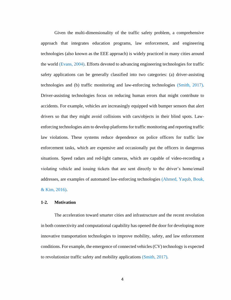
Given the multi-dimensionality of the traffic safety problem, a comprehensive
approach that integrates education programs, law enforcement, and engineering
technologies (also known as the EEE approach) is widely practiced in many cities around
the world (Evans, 2004). Efforts devoted to advancing engineering technologies for traffic
safety applications can be generally classified into two categories: (a) driver-assisting
technologies and (b) traffic monitoring and law-enforcing technologies (Smith, 2017).
Driver-assisting technologies focus on reducing human errors that might contribute to
accidents. For example, vehicles are increasingly equipped with bumper sensors that alert
drivers so that they might avoid collisions with cars/objects in their blind spots. Law-
enforcing technologies aim to develop platforms for traffic monitoring and reporting traffic
law violations. These systems reduce dependence on police officers for traffic law
enforcement tasks, which are expensive and occasionally put the officers in dangerous
situations. Speed radars and red-light cameras, which are capable of video-recording a
violating vehicle and issuing tickets that are sent directly to the driver’s home/email
addresses, are examples of automated law-enforcing technologies (Ahmed, Yaqub, Bouk,
& Kim, 2016).
1-2. Motivation
The acceleration toward smarter cities and infrastructure and the recent revolution
in both connectivity and computational capability has opened the door for developing more
innovative transportation technologies to improve mobility, safety, and law enforcement
conditions. For example, the emergence of connected vehicles (CV) technology is expected
to revolutionize traffic safety and mobility applications (Smith, 2017).

5
Current research and development efforts focus on leveraging vehicle-to-vehicle
(V2V) and vehicle-to-infrastructure (V2I) communications to enhance traffic safety by
providing better driving assistance capabilities. For example, dedicated short-range
communication (DSRC) channels for vehicular communications have enabled the
development of warning systems that keep drivers aware of their 360° surroundings. In
addition, CV technology has been proposed to harmonize the traffic speed on freeways and
to provide early warnings for drivers about building downstream queues from their current
locations (Talebpour, Mahmassani, & Hamdar, 2013). It is generally estimated that CV
technology could eliminate or mitigate up to 80 percent of minor crashes that take place at
intersections, parking lots, or during lane changes by enabling drivers to receive warning
messages through V2V and V2I communications (NHTSA, 2016). According to the
National Highway Traffic Safety Administration (NHTSA), this technology could have
averted, on average, half a million crashes, a quarter of a million injuries, and the deaths of
one thousand Americans in 2017 (NHTSA, 2017).
Effort devoted to adopting CV technology for law enforcement applications is in
its infancy. The idea is to integrate CV technologies in law-enforcement vehicles, as shown
in Figure 1-3, to improve data gathering, processing, and tracking of surrounding vehicles,
with the goal of easing and increasing the efficiency of police officers’ jobs (Microsoft ,
2015).

6
Figure 1-4: The Microsoft advanced patrol platform (Source: (Eichner, 2017; Surur, 2018)
While the concerns about privacy invasion and lack of supporting legislation have
slowed market readiness for these applications, there are strong indications that CV
technology could benefit such applications. For example, automobile insurance companies
have recently shown interest in using a CV to develop systems for monitoring and profiling
drivers’ performance in terms of several driving aggressiveness measures (e.g., frequent
lane changing, speeding, acceleration and deceleration rates, etc.). Obtaining this
information enables insurance companies to design customized insurance policies with
minimum loss risk (Händel, et al., 2014). In addition, there has been considerable debate
over current traffic penalties for violators of traffic laws which include warnings, fines,
driver’s license suspensions, and jail time and their effectiveness for curbing worsening
trends in traffic law compliance. Intensive research in the last fifty years has concluded
that improvements in future traffic conditions will depend on improving both driver
performance and driver behavior (Lee, 2008).
7
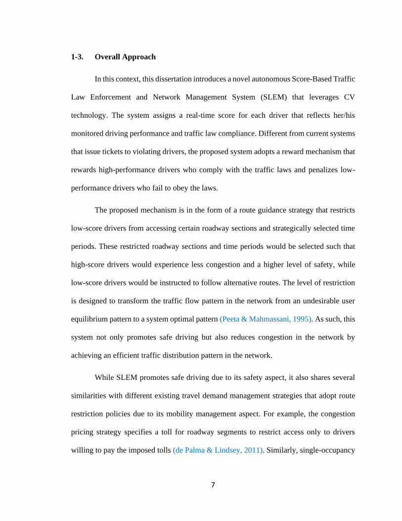
1-3. Overall Approach
In this context, this dissertation introduces a novel autonomous Score-Based Traffic
Law Enforcement and Network Management System (SLEM) that leverages CV
technology. The system assigns a real-time score for each driver that reflects her/his
monitored driving performance and traffic law compliance. Different from current systems
that issue tickets to violating drivers, the proposed system adopts a reward mechanism that
rewards high-performance drivers who comply with the traffic laws and penalizes low-
performance drivers who fail to obey the laws.
The proposed mechanism is in the form of a route guidance strategy that restricts
low-score drivers from accessing certain roadway sections and strategically selected time
periods. These restricted roadway sections and time periods would be selected such that
high-score drivers would experience less congestion and a higher level of safety, while
low-score drivers would be instructed to follow alternative routes. The level of restriction
is designed to transform the traffic flow pattern in the network from an undesirable user
equilibrium pattern to a system optimal pattern (Peeta & Mahmassani, 1995). As such, this
system not only promotes safe driving but also reduces congestion in the network by
achieving an efficient traffic distribution pattern in the network.
While SLEM promotes safe driving due to its safety aspect, it also shares several
similarities with different existing travel demand management strategies that adopt route
restriction policies due to its mobility management aspect. For example, the congestion
pricing strategy specifies a toll for roadway segments to restrict access only to drivers
willing to pay the imposed tolls (de Palma & Lindsey, 2011). Similarly, single-occupancy

8
vehicles are restricted from traveling on high occupancy vehicle (HOV) lanes
(Abdelghany, Abdelghany, Mahmassani, & Murray, 2000; Murray, Mahmassani, &
Abdelghany, 2001). The road rationing strategy adopted in several cities is another
example of route restriction strategy, where vehicles are restricted from accessing some
roads based upon the last digits of the license plate number on certain established days
during certain periods (Han, Yang, & Wang, 2010). In addition, the credit-based policy can
be viewed as a restriction strategy, where each driver maintains a travel credit beyond
which drivers are not allowed to travel in the network (Kockelman & Lemp, 2011). Finally,
the incentive-based demand management strategy aims to reduce access to congested
routes by providing incentives to drivers to avoid these routes (Ben-Elia & Ettema, 2011a).
Although these strategies have shown to be effective in reducing traffic congestion, their
justice and equity remain an issue of heated debate.
1-4. Research Objectives and Contributions
Because of the novelty of SLEM, this dissertation focused on two objectives. First,
to understand both public acceptance and the opinion of traffic system
experts/professionals regarding the adoption of SLEM in their regions. To obtain
information on public acceptance, a national survey with a sample of 1,418 participants
was designed and distributed across all 50 states and the District of Columbia (DC). The
survey collected information on the participants’ socioeconomic characteristics, their
driving performance history, and their level of acceptance of the new system. Using this
sample data, a logistic regression model was developed to determine significant variables
that affect public acceptance of SLEM and to predict its level of acceptance under different
policy and operation scenarios. Another survey was implemented at smaller scale to gather
9
information on the views of traffic system experts/professionals of SLEM. The sample
included experts from public agencies and consultants providing services to these agencies.
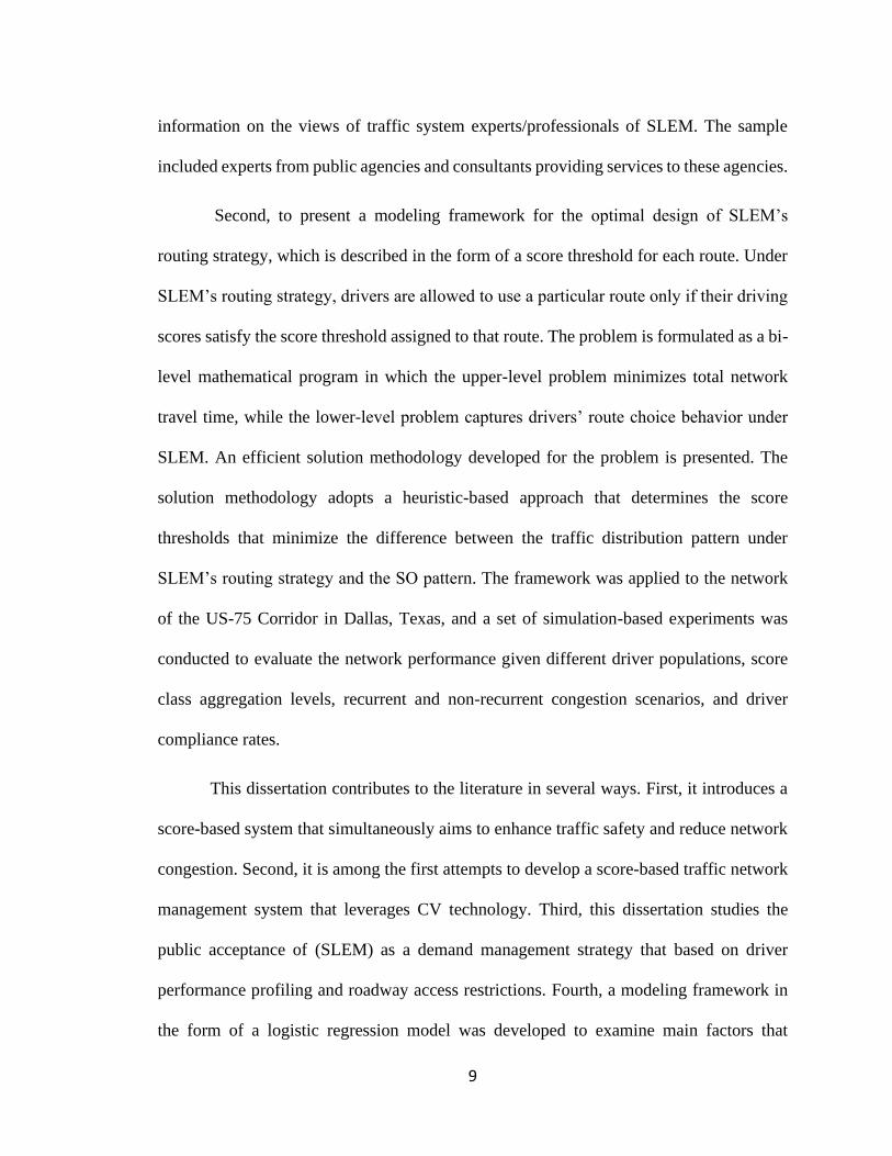
Second, to present a modeling framework for the optimal design of SLEM’s
routing strategy, which is described in the form of a score threshold for each route. Under
SLEM’s routing strategy, drivers are allowed to use a particular route only if their driving
scores satisfy the score threshold assigned to that route. The problem is formulated as a bi-
level mathematical program in which the upper-level problem minimizes total network
travel time, while the lower-level problem captures drivers’ route choice behavior under
SLEM. An efficient solution methodology developed for the problem is presented. The
solution methodology adopts a heuristic-based approach that determines the score
thresholds that minimize the difference between the traffic distribution pattern under
SLEM’s routing strategy and the SO pattern. The framework was applied to the network
of the US-75 Corridor in Dallas, Texas, and a set of simulation-based experiments was
conducted to evaluate the network performance given different driver populations, score
class aggregation levels, recurrent and non-recurrent congestion scenarios, and driver
compliance rates.
This dissertation contributes to the literature in several ways. First, it introduces a
score-based system that simultaneously aims to enhance traffic safety and reduce network
congestion. Second, it is among the first attempts to develop a score-based traffic network
management system that leverages CV technology. Third, this dissertation studies the
public acceptance of (SLEM) as a demand management strategy that based on driver
performance profiling and roadway access restrictions. Fourth, a modeling framework in
the form of a logistic regression model was developed to examine main factors that

10
influence public acceptance of the real-world deployment of the system. Fifth, this
dissertation presents a modeling framework consisting of a mathematical formulation and
an efficient solution methodology to design SLEM’s optimal route guidance strategy.
Finally, this dissertation quantifies the travel time savings associated with deploying SLEM
in a real-world network.
1-5. Dissertation Organization
The remainder of this dissertation is organized as follows. The next chapter reviews
different topics related to SLEM, including the history of performance-based driver
profiling and the development of score-based systems. The survey design, methods, and
the procedure of the data preparation is given in Chapter 3. In Chapter 4, the results of the
surveys and discusses the data analysis and findings of the developed logistic regression
model are presented. The problem definition and the set of assumptions are introduced in
chapter 5 followed by the solution methodology in Chapter 6. The experimental results and
analysis are presented in Chapter 7 of SLEM. Finally, the conclusion and future research
is given in the final chapter, Chapter 8.
11
Chapter 2
REVIEW OF THE LITERATURE
2-1. Introduction
Considering the multi-faceted nature of SLEM, the main objective of this chapter
is to review two related topics in the literature: (I) recent advances in driver performance
profiling using telematics technologies, and (II) travel demand management strategies that
share similarity with SLEM. These two topics share several traffic safety and mobility
policies and applications introduced in the literature. For traffic safety, this chapter reviews
the major approaches proposed in the literature, which largely concern driver profiling and
monitoring. Regarding traffic mobility, this chapter reviews the major traffic management
policies proposed in the literature that focus on roadway access restriction.
2-2. Driver Behavior Profiling and Monitoring
Advances in telematics technology have focused considerable attention on the
concept of monitoring and profiling drivers based on their driving performance for several
applications, such as vehicle insurance and commercial/public transportation safety. For
example, automobile insurance companies have recently introduced the Usage-Based
Insurance (UBI) model, which issues insurance policies to drivers that reflect their vehicle
usage and other known information concerning their driving performance.
12
In addition, several technology companies have proposed a scoring system that can
be used by owners of commercial vehicles and public transportation agencies to evaluate
the performance of their drivers. As proposed in (Händel, et al., 2014), these scores
combine several metrics that are monitored in real-time (e.g., acceleration and braking,
speeding, smoothness, swerving, etc.). For instance, the AXA Drive Coach application was
developed to sense and analyze vehicle maneuvers, then assign scores to drivers based on
these patterns (Tardy, 2015).
Another driver scoring application, DriveSafe, applies pattern recognition
techniques to detect driver distraction (Bergasa, Almería, Almazán, Yebes, & Arroyo,
2014). Inspired by financial credit scores, the credit scoring services company FICO
recently announced a new product called FICO® Safe Driving Score to establish a new
driver characterization system that categorizes drivers based on their driving performance
(FICO, 2018).
Three main approaches are used to monitor driving performance: physiological, in-
vehicle sensing, and performance-based. The physiological-based approach is mainly used
to evaluate the performance of commercial drivers. Sensors are physically attached to the
drivers’ bodies to acquire different bio-measures that can be used to assess the drivers’
level of alertness or fatigue. Examples of these bio-measures include an
electroencephalogram (EEG, brain activity), an electrooculogram (EOG, eye movement),
and an electrocardiogram (ECG, heart rate) (Borghini, Astolfi, Vecchiato, Mattia, &
Babiloni, 2014). However, this approach is not widely accepted because drivers feel
uncomfortable with these sensors attached to their bodies, especially if they are driving for
long distances.

13
The in-vehicle sensing approach aims to monitor drivers’ alertness and evaluate
their ability to maintain safe driving by installing sensors in the vehicle rather than
attaching them to the drivers’ bodies. For example, (Liang, Reyes, & Lee, 2007) developed
a platform to detect distracted drivers by monitoring eye movement and driving
performance in a simulation environment. (Cyganek & Gruszczyński, 2014) performed
field experiments to detect drivers’ fatigue and drowsiness. (Mbouna, Kong, & Chun,
2013) examined visual feature monitoring schemes that monitor a driver’s pupil and head
position to detect drowsiness and distraction.
Furthermore, a driver distraction detection experiment was conducted by (Vicente,
et al., 2015),that monitored the driver’s head pose and gaze. In addition to distraction and
drowsiness, detection of the driver’s emotional stress was also proposed by (Gao, Yüce, &
Thiran, 2014), wherein facial recognition sensing was used to detect a driver’s
psychological state. An artificial neural network model was developed by (Ye, Osman,
Ishak, & Hashemi, 2017) to predict the driver’s involvement in secondary distracting tasks
such as calling, texting, and passenger interaction. Driving performance is also inferred by
analyzing acceleration and braking pedal operations (Wahab, Quek, Tan, & Takeda, 2009).
The IntelliSafe system introduced by Volvo is an example of a driver alertness detection
system deployed in the real world (VOLVO, 2018).
Finally, performance-based approaches monitor the vehicle’s movements to assess
driver performance. For example, vehicle movement data are used to infer information
from the driver’s braking and acceleration (Pentland & Liu, 1999) as well as lane changing
and maneuvering (Kuge, Yamamura, Shimoyama, & Liu, 2000). (Gonzalez, Wilby, Diaz,
& Avila, 2014) developed a model that detects driver aggressiveness by monitoring lateral
14
and longitudinal accelerations and speed. Car following and headway distance data are also
considered to measure driving aggressiveness (Miyajima, et al., 2007).
The majority of the literature views the smartphone as the most affordable
telematics tool for monitoring driver performance. Data on driving patterns could be
acquired from the drivers’ smartphones (e.g., accelerometers, magnetometers, GPS) to
detect their risky performance and aggressiveness (Eren, Makinist, Akin, & Yilmaz, 2012;
Hong, Margines, & Dey, 2014). These data can also be used to reveal additional
information regarding the alertness of the driver (Dai et al., 2010). Smartphone applications
have been developed to detect the activities of drivers and provide real-time suggestions to
enhance their performance (Araújo et al., 2012).
Evaluating the accuracy of driving performance systems that use smartphone data
is already underway. For example, Paefgen et al. (2012) conducted a field study to evaluate
a smartphone application for the assessment of driving performance during critical driving
events and found that smartphones tend to overestimate the measurements of critical
driving events. Castignani et al. (2013) considered an application for UBI driving scores
and found that more effort is required to improve the accuracy of data gathered by
smartphones. This work was extended by Castignani et al. (2015), who explored the
SenseFleet drivers’ profiling and scoring platform to detect risky driving events based on
data that were collected independently from both a mobile device and the vehicle.
Experimental results showed that SenseFleet was accurate in terms of differentiating
between risky and calm driving.

15
More recently, CV technology has been looked at as a plausible technology for
monitoring and profiling driving performance (Chen et al., 2018). Based on data collected
from a simulated CV platform, a machine-learning algorithm was proposed to profile
drivers in terms of driving aggressiveness and assign them performance scores. The results
from the developed model suggest that low-score drivers should follow safe drivers in order
to enhance highway safety and mobility conditions.
2-3. Travel Demand Management
Enormous efforts have been devoted to developing effective solutions to curb the
worsening traffic congestion problem and its adverse consequences. Specifically, two main
approaches are widely considered to manage traffic congestion in urban areas – namely,
network capacity management (NCM) and travel demand management (TDM). For NCM,
traffic congestion is tackled by enhancing the roadway network capacity. NCM strategies
include, for example, dynamic signal timing (Teklu, Sumalee, & Watling, 2007), active
ramp metering (Papageorgiou & Kotsialos, 2002; Cassidy & Rudjanakanoknad, 2005),
variable speed limits (Talebpour, Mahmassani, & Hamdar, 2013; Khondaker & Kattan,
2015), and hard shoulder utilization during incidents (Lemke, 2010). These strategies are
usually deployed in the form of integrated traffic management schemes at the corridor and
regional levels (Zhou, Mahmassani, & Zhang, 2008; Hashemi & Abdelghany, 2016).
TDM, on the other hand, aims to change commuters’ behavior with the goal of
achieving a better temporal and spatial traffic distribution in the network (Meyer, 1999).
Travelers are encouraged to reduce dependence on their private cars, schedule their travel
during off-peak periods, and travel on less congested routes. Examples of TDM strategies
16
include congestion and dynamic parking pricing (Tsekeris & Voß, 2009; de Palma &
Lindsey, 2011), traveler information provision (Ben-Akiva, De Palma, & Isam, 1991;
Mahmassani & Liu, 1999; Hashemi & Abdelghany, 2018), flexible working hours (Kim,
Choo, & Mokhtarian, 2015), and incentives for carpooling and ridesharing (Daganzo &
Cassidy, 2008), to name a few. A common tactic among most TDM strategies is to
implicitly restrict, or inconvenient, a portion of the travelers for using their private cars
along certain routes/facilities/zones during the peak periods in such a way that congestion
is reduced. While the approach has shown to be effective in influencing traveler behavior
and reducing traffic congestion, TDM strategies – especially those that are financial-based
– have encountered public resistance due to travel equity concerns (Gärling & Schuitema,
2007; Viard & Fu, 2015).
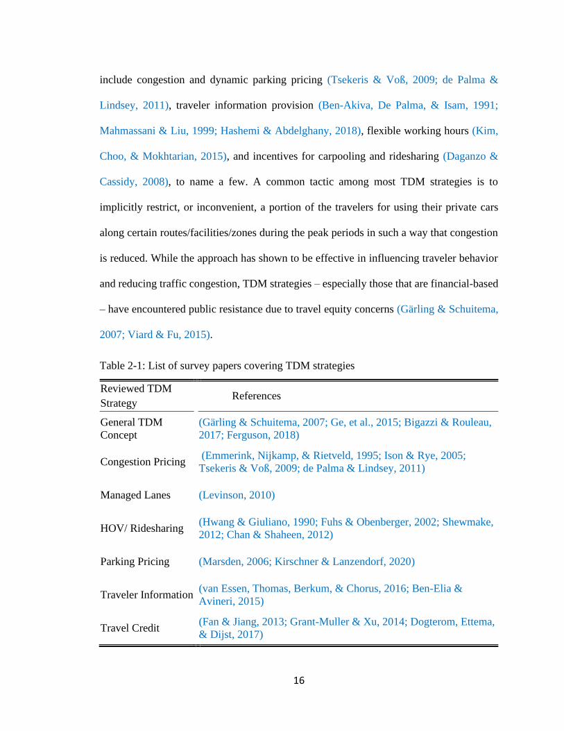
Table 2-1: List of survey papers covering TDM strategies
Reviewed TDM
Strategy References
General TDM
Concept
(Gärling & Schuitema, 2007; Ge, et al., 2015; Bigazzi & Rouleau,
2017; Ferguson, 2018)
Congestion Pricing (Emmerink, Nijkamp, & Rietveld, 1995; Ison & Rye, 2005;
Tsekeris & Voß, 2009; de Palma & Lindsey, 2011)
Managed Lanes (Levinson, 2010)
HOV/ Ridesharing (Hwang & Giuliano, 1990; Fuhs & Obenberger, 2002; Shewmake,
2012; Chan & Shaheen, 2012)
Parking Pricing (Marsden, 2006; Kirschner & Lanzendorf, 2020)
Traveler Information (van Essen, Thomas, Berkum, & Chorus, 2016; Ben-Elia &
Avineri, 2015)
Travel Credit (Fan & Jiang, 2013; Grant-Muller & Xu, 2014; Dogterom, Ettema,
& Dijst, 2017)

17
Several articles have been dedicated to reviewing TDM strategies, as shown in
Table 2-1. These articles either focus on the overall TDM concept or one of the individual
strategies widely adopted in congested urban areas. This chapter extends these efforts by
providing an updated review of the class of TDM strategies that adopt roadway access
restriction to influence traveler behavior. The review provides a summary of economic and
environmental benefits reported for these strategies, innovations in their theories and
supporting technologies, and common issues/obstacles associated with adopting these
strategies, such as equity concerns and public acceptance. Over 300 references were
collected and reviewed. These references were identified using a rich collection of
keywords. Figure 2-1 gives common keywords identified in these references as the result
of text-mining their titles and abstracts, where the size of the word represents its popularity
in the collected references. As shown in the figure, the words ‘congestion’, ‘pricing’ and
‘lanes’ are highly mentioned, implying the popularity of congestion pricing and managed
lanes TDM strategies. These references are grouped under six main categories with respect
to the mechanism used to restrict roadway access. These main categories include financial-
, priority-, categorization-, incentive-, credit-, and performance-based. The references of
three of these six categories are further classified into two or three classes resulting in a
total of 10 categories.
Figure 2-2 illustrates the 10 categories used for classifying the collected literature.
The figure also gives the milestone references for each class, which are identified based on
their average number of citations per year since publication using citation data from Google
Scholar retrieved in February 2nd, 2020. A branch in the figure indicates one category,
while the circle leaves are the milestone references of that category. Ten leaves are

18
considered under each branch, representing the top ten highly cited references. The size of
a leaf represents the number of citations of its reference, which ranges from 99 to 2 citations
per year. This chapter is organized as follows: Sections 2 to 7 review each of the six main
TDM strategies mentioned above, followed by Section 8 which provides a summary and
concluding remarks.
Figure 2-1: Popular keywords used in the collected references

19
Figure 2-2: Different categories of state-of-the-art demand management strategies
2-3-1. Congestion Pricing
Financial restriction is when drivers must pay monetary fees to enter a congested
area. Road pricing has been widely investigated and could be traced back to (Buchanan,
1952; Beckmann et al., 1956; Walters, 1961; Vickrey W. S., 1963). It was first officially
introduced in London, UK in the early 1960s in a proposal report to the Ministry of
Transport in the United Kingdom (Smeed, 1964). This dissertation introduced congestion
pricing to enter the central London zone. That scheme was not accepted by policymakers,

20
who preferred another scheme that involved parking taxation within central London zone
(Thomson, 1967). In 1975, Singapore became the first country to implement a congestion
pricing scheme using basic technology systems and in 1998, they introduced a fully
automated charging system (FHWA, 2008). In 2003, London implemented a congestion
charge downtown during peak hours to reduce congestion and traffic jams (Banister, 2003).
Since the 1990s, researchers have investigated congestion pricing from multiple
points of view. Intensive research has been conducted to evaluate the acceptability
(Jakobsson et al., 2000; Schade & Schlag, 2003) and equity of congestion pricing
(Levinson, 2011). Congestion pricing has different forms, including lane-based, highway
(facility)-based, and, the most common type, the cordon (zone) based-pricing (FHWA,
2018). The rise of congestion pricing prompted researchers to study different types and
aspects of congestion pricing, including economic aspects, feasibility, environmental
impact, and impact on driving behavior.
The first body of research considered precisely the economic aspects of the
congestion pricing approach. Arnott & Small (1994) predicted that congestion cost would
be tens of billions of dollars in large metropolitan regions. Small (1992) and Eliasson &
Mattsson (2006) discussed how to use the revenue generated from the congestion pricing
after implementation and suggested tax reduction, alternative transportation development,
and infrastructure improvement. Calfee & Winston (1998) studied the amount commuters
are willing to pay to save time-based on their income and found that the value is low and
independent from traffic conditions. Eliasson (2016) discussed the fairness of congestion
pricing from consumer and citizen perspectives using data from people with different
income in four European cities.
21
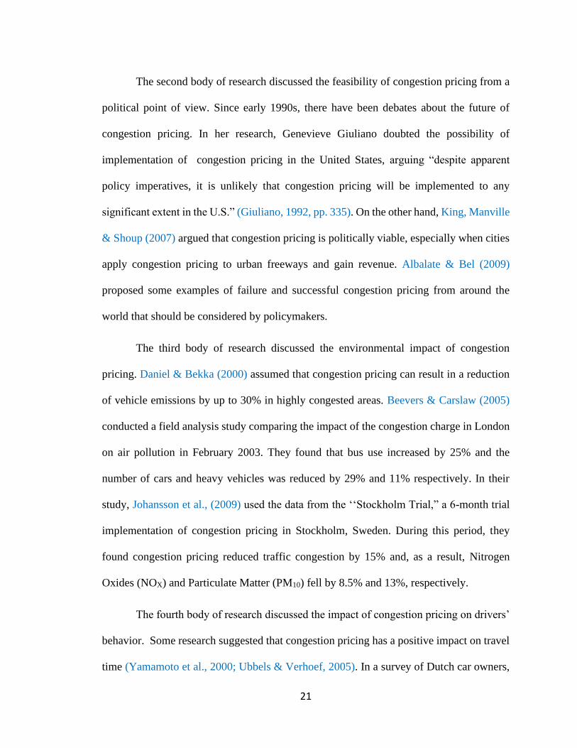
The second body of research discussed the feasibility of congestion pricing from a
political point of view. Since early 1990s, there have been debates about the future of
congestion pricing. In her research, Genevieve Giuliano doubted the possibility of
implementation of congestion pricing in the United States, arguing “despite apparent
policy imperatives, it is unlikely that congestion pricing will be implemented to any
significant extent in the U.S.” (Giuliano, 1992, pp. 335). On the other hand, King, Manville
& Shoup (2007) argued that congestion pricing is politically viable, especially when cities
apply congestion pricing to urban freeways and gain revenue. Albalate & Bel (2009)
proposed some examples of failure and successful congestion pricing from around the
world that should be considered by policymakers.
The third body of research discussed the environmental impact of congestion
pricing. Daniel & Bekka (2000) assumed that congestion pricing can result in a reduction
of vehicle emissions by up to 30% in highly congested areas. Beevers & Carslaw (2005)
conducted a field analysis study comparing the impact of the congestion charge in London
on air pollution in February 2003. They found that bus use increased by 25% and the
number of cars and heavy vehicles was reduced by 29% and 11% respectively. In their
study, Johansson et al., (2009) used the data from the ‘‘Stockholm Trial,” a 6-month trial
implementation of congestion pricing in Stockholm, Sweden. During this period, they
found congestion pricing reduced traffic congestion by 15% and, as a result, Nitrogen
Oxides (NOX) and Particulate Matter (PM10) fell by 8.5% and 13%, respectively.
The fourth body of research discussed the impact of congestion pricing on drivers’
behavior. Some research suggested that congestion pricing has a positive impact on travel
time (Yamamoto et al., 2000; Ubbels & Verhoef, 2005). In a survey of Dutch car owners,
22
Albert & Mahalel (2006) evaluated and compared peoples’ attitudes towards congestion
pricing and found that it has a positive impact on driving behavior. Simićević et al., (2013)
hypothesized that parking has an impact on driving behavior and they developed a model
to predict the effect of changing parking price and time limits on drivers’ behavior. It
showed that parking price affected car usage, while time limitations affected driver’s
choice in terms of parking type (on-street or off-street parking).
2-3-2. Parking Pricing
Many other researchers have also investigated the effects of parking pricing (Glazer
& Niskanen, 1992; Anderson & de Palma, 2004; Arnott & Inci, 2006; Inci, 2015). The first
group of research investigated the impact of parking on congestion. Arnott et al., (1991)
assessed relative efficiency of road tolls and parking pricing in a central business district
(CBD) and found that parking was inefficient. Other research suggested that parking fees
can be a substitute for road pricing (Verhoef et al., 1995). The second group of research
studied the effect of parking pricing on welfare. (Glazer & Niskanen, 1992; Borger &
Wuyts, 2009; Proost & Dender, 2008; Arnott & Inci, 2006). The third group of research
assumed that cruising for parking is the main cause of congestion. Shoup (2004) found that
the average time cruising to find a parking space was 3-14 minutes. Arnott & Rowse,
(1999) estimated that 50% of cars driving in downtown in cities such as Boston and large
European cities are cruising for parking. The fourth group discussed the economic loss of
cruising for parking. In Amsterdam, Netherlands the cruising cost is estimated to be 1 Euro
per day where the citizens are willing to pay 10 Euros daily for parking permit (Ommeren
et al., 2011). Using a nationwide random sample of car trips, a Netherlands-based study
showed that when parking pricing was implemented for both on-street and off-street

23
parking, the average cruising time was only 36 seconds (Ommeren & Derk Wentink, 2012).
In San Francisco, CA, the SFpark project was launched in 2011 with a 60-80 percent target
occupancy rate (SFMTA, 2014). Evaluation studies show that during the first two years
(2011-2013), SFpark achieved its goal of 60-80 percent occupancy for metered parking
(Millard-Ball et al., 2014; Chatman & Manville, 2014). Furthermore, the two-year
evaluation of SFpark showed a 50% drop in cruising (Millard-Ball et al., 2014).
Further research discussed other aspects of congestion pricing. For instance, Chen
et al., (2016) proposed time of day congestion pricing based on vehicle mileage traveled
(VMT) on freeways to tackle congestion and generate revenue. Considering an
autonomous vehicles (AV) environment, recent work by Simoni et al., (2019) examined
the effect of different congestion pricing and tolling strategies scenarios on traffic
congestion and welfare.
2-4. Reservation (Priority)-Based Restriction
2-4-1. High Occupancy Vehicles (HOV)
Reservation or “priority” based traffic management is another main traffic
restriction strategy which aims to manage traffic demand. The increase in the number of
vehicles with single occupancy has resulted in an increase in traffic congestion and
pollution (Caulfield, 2009). This has raised concern among policymakers and urged them
to encourage drivers to carpool. The idea of High Occupancy Vehicle (HOV) lanes was
developed initially from the bus-only lane on the Henry G. Shirley Memorial Highway (I-
395) in the Washington D.C. metropolitan area in 1969 (Turnbull, 1992). In 1973, the bus-
only lane became the first HOV lane for passenger cars (Leman et al., 1994). In 2012, the

24
number of HOV lanes in the U.S. was 126 in 27 metropolitan areas with a total length of
over 1000 miles (Metro, n.d.). The 2013 edition of the American Community Survey
(ACS) conducted by the U.S. Census Bureau showed that about 76.4 percent of Americans
drive alone (McKenzie, 2015). The same report also showed historic data about carpooling,
which clearly demonstrated that the percentage of solo drivers has been increasing.
Between 1980 and 2013, the total number of employees commuting by cars
increased by only about 1.7 percent from 84.1 percent to 85.8 percent, while single-
occupancy vehicles increased by about 12 percent, from 64.4 percent to 76.4 percent
(McKenzie, 2015). The same report also showed that carpoolers decreased dramatically
during the same period, from 19.7 percent to 9.4 percent (McKenzie, 2015). The underuse
of the HOV lanes led researchers to evaluate their effectiveness for mobility in the U.S.
(Turnbull et al., 1991; Giuliano et al., 1990). Kwon & Varaiya (2008) conducted a
California-based study showing that the goals of HOV lanes were not met. In addition,
Poole & Balaker (2005) show that HOV 2+ lanes led to drivers to avoid vanpool, which
originally established HOV lanes, and that these lanes benefitted mostly from family
members who were already carpooling. Fielding & Klein (1993) concluded that about 43
percent of carpoolers are members of the same household and therefore, HOV lanes need
modification to be more effective. Furthermore, Orski (2001) showed that HOV lanes have
not changed driving habits in the U.S. Dahlgren (1998) also shows that in most cases,
adding an additional general-purpose lane is more effective than constructing an HOV lane
in terms of reducing travel delay. In terms of social welfare, Yang & Huang (1999) showed
that current HOV practices do not maximize social welfare and incentives should be
provided for HOV lane users.
25
Daganzo & Cassidy (2008) investigated the effect of HOV lanes on congestion,
implemented a city-wide HOV lane network, and made recommendations to consider a
city-wide bus lane system. From a safety point of view, Golob et al., (1989) conducted a
14-month study on State Freeway Route 91 (State Route-91) in Riverside, California to
compare the characteristics and frequencies of accidents with and without physical
separation between general purpose and HOV lanes. Jang et al., (2009) also evaluated the
safety of HOV lanes by comparing continuous and limited freeway access and found that
limited access does not have safety advantages over continuous access HOV lanes.
Researchers also evaluated the environmental impact of the HOV lanes. Johnston
& Ceerla (1996) developed an evaluation of the travel and emission impact of new HOV
lanes under the Federal Clean Air Act (CAA) and found that HOV lanes might increase
both vehicles’ travel distance and emission. Boriboonsomsin & Barth (2007) compared
HOV lanes and mixed flow lanes’ contribution to emissions and they found that HOV lanes
produce less emission mass on a per-lane basis. In another study conducted in different
parts of California, Boriboonsomsin & Barth (2008) also compared continuous and limited
HOV access on freeways in terms of vehicle emission using a simulation approach and
found that continuous access HOV lanes produce a lower level of pollutant emissions.
2-4-2. High Occupancy Tolls (HOT)
The underuse of the HOV lanes led many researchers to investigate other
alternatives to improve the effectiveness of HOV lanes and traffic networks in general.
Fielding & Klein (1993) proposed the idea of converting the current HOV lanes to High
Occupancy Tolls (HOT). To utilize more of the lane’s capacity, Fielding & Klein (1993)
suggested HOV 3+, while all other vehicles could have access if they paid the peak-hour

26
toll. The implementation of HOV 3+ lanes started in a 10-mile-long, four-lane segment in
the median of the Riverside Freeway (State Route 91) located in Orange County, CA on
December, 27 1995 (Sullivan, 2000). HOT lanes became a hot topic and promising solution
to adopt for three main reasons: increased utility of underused HOV lanes, revenue
generated, and political feasibility (Poole & Orski, 2000; Konishi & Mun, 2010).
A mesoscopic simulation study using DYNASMART traffic simulation-
assignment model was conducted by Abdelghany, et al., (2000) to evaluate HOT lanes
under different designs and operation schemes. Dahlgren (2002) constructed a model to
determine the locations where HOV, HOT, and/or mixed flow would be most effective to
reduce travel delay. A Washington, DC-based study implemented by Safirova et al., (2003)
showed that HOT lanes are promising and would increase utilization of HOV lanes while
generating revenue. Mastako et al., (1998) studied the change in commuters’ behavior after
the implementation of HOT in State Route 91, finding that the HOV commuters increased
from 20 percent to 29 percent.
Another impact of switching to HOT that researchers examined was the welfare
effect. Small et al., (2006) conducted a simulation-based study of the two-lane California
State Route 91, performing a welfare analysis based on different toll, HOV, and HOT
policies. They found that in case of one leaving one lane free, the HOT would result in best
welfare gain, with a gain of $2.25 per person. In a case of two-lane strategy, the toll seem
to be the best practice to increase welfare with a $2.99 gain. In addition, Konishi & Mun
(2010) examined the welfare effect of HOV and HOT lanes and whether converting to
HOT would improve efficiency of road use. Furthermore, Safirova, et al. (2004) conducted
another Washington based study to compare the welfare effect of different pricing

27
strategies and found that HOT has a superior advantage over traditional pricing strategies
in terms of welfare gain.
The safety impact of HOT has also been examined by some researchers. Cao et al.,
(2012) studied the change in accident rate after converting HOV to HOT on the interstate
I-349 and found that the conversion reduced the crash rate by 5.3 percent.
2-4-3. Highway Inventory Booking
Over the years, prioritizing “reserving” highways for certain drivers has been
widely discussed and was improved and extended to include different traffic management
strategies other than HOV and HOT lanes. Booking-based traffic demand management is
a strategy that allows drivers to book a slot on the highway for their vehicle to access during
their trips. it has been widely investigated and although potential advantages and feasible
to implement exist, serious political and social acceptance can be a major obstacle
(Buitelaar et al., 2007). A highway booking system was first proposed in Akahane &
Kuwahara (1996) as part of a survey study to measure the benefits of the trip reservation
system to manage the highways during holiday seasons. Wong (1997) proposed a
qualitative approach for a highway slot booking system and discussed the advantages of
such systems. Koolstra (1999) conducted a theoretical study to estimate the potential
benefits of a highway slot booking system by analyzing the difference between user-
equilibrium (UE) and system optimal (SO) in terms of departure time.
To measure the effectiveness of the highway booking strategy, Feijter et al. (2004)
conducted a simulation study which showed that trip booking has a positive impact on
travel time. Teodorovic et al. (2005) proposed a model of the highway space inventory

28
control system (HSICS) where all users have to make a reservation in advance to enter the
highway. Their system allows traffic operators to make real-time decisions to accept or
reject reservation requests. In their model, they assume a constant average speed and did
not consider traffic flow characteristics, which resulted in limitations to the model’s
accuracy in terms of the number of vehicles on each link at every time interval. Edara &
Teodorovic (2008) improved the accuracy of the original model proposed in Teodorovic et
al. (2005) by replacing the average constant speed with a link-specific mean speed that is
estimated using the Green-Shields speed-density relationship.
Other research used the highway booking strategy as an area -or time-specific
strategy. For example, Zhao et al., (2010) assumed an area-based booking system such that
all vehicles willing to enter the downtown area are required to make reservations in
advance. An integer programming formulation was modeled to obtain the optimal mix of
vehicles based on different characteristics such as occupancy, departure time, and trip
duration. Liu et al., (2015) assumed a time-based reservation system such that the system
allocates the highway slots to potential users during different time intervals. Based on the
highway capacity and the number of reservations made, the system will determine whether
to accept or reject a request.
Other reservation methodologies have also been proposed. A token-based highway
reservation system was proposed by Liu et al. (2013) and concluded that the token system
showed advantages in terms of traffic throughput, density, and speed. Teodorovićet al.
(2008) proposed another methodology of highway booking called auction-based
congestion pricing. The basic idea of auction-based congestion pricing is that drivers who
want to enter the downtown area during a specific time period will need to participate in
29
an auction to reserve a space where the authorities will determine whether or not to accept
their bids.
2-5. Vehicle Characteristics-Based Restriction
2-5-1. Truck Restriction
The expansion in trade and e-commerce in the U.S. resulted in an increase in
logistics and supply chain operations. In fact, the top 100 U.S. metro areas (~ 12 percent
land area) hold 80 percent of trade, 75 percent of GDP, and 66 percent of the population
(Tomer & Kane, 2014). The increased number of heavy trucks on highways has raised
concerns among researchers and policymakers regarding their negative impact, especially
their lower speeds. Slower vehicles in general have stimulated the interests of many
researchers. Gazis & Herman, (1992) were the first to investigate the negative impact of
slow vehicles and they proposed a model to measure the effect of a slower vehicle, calling
this phenomenon a “moving bottleneck” as a queue is starting to form. Newell, (1993) and
Newell, (1998) proposed a more complete model where they studied the effects of a single
slow convoy or vehicle on a two-lane highway based on the Lighthill-Whitham-Richards
(LWR) theory (Lighthill & Whitham, 1955; Richards, 1956). Newell introduced the
kinematic wave theory of moving bottleneck (KW-MB) and studied its influence on a
traffic system. Newell also investigated the consequences of trucks on steep grades. In this
theory, Newell assumes that any vehicle that travels slower than the traffic stream is
becoming an active moving bottleneck. A second complete model was proposed by
Lebacque et al., (1998), who provided a simple model of the interaction between slower
vehicles (buses) and the surrounding traffic flow based on the first-order macroscopic
model of the (LWR) theory. A third complete model was proposed in Muñoz & Daganzo,
30
(2002) where they performed a freeway observational experiment and validation of
Newell’s (KW-MB) theory. Leclercq et al., (2004) proposed a unified general framework
for the moving-bottleneck models based on the Lighthill, Whitham and Richards theory.
Additionally, Kerner & Klenov, (2010) provided an analysis of the moving bottleneck
based on the three-phase traffic theory which was developed by (Kerner, 2009).
In addition to the analytical models, numerical models have also been developed in
order to solve the moving bottleneck issue. Building on their first model proposed in
Lebacque et al., (1998), they developed another numerical model in 2002 (Giorgi et al.,
2002). In addition, Daganzo & Laval, (2005a) and Daganzo & Laval, (2005b) proposed a
complete and accurate numerical model solution to the bottleneck problem which later
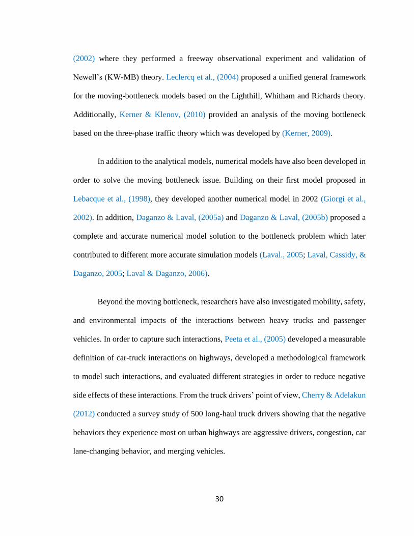
contributed to different more accurate simulation models (Laval., 2005; Laval, Cassidy, &
Daganzo, 2005; Laval & Daganzo, 2006).
Beyond the moving bottleneck, researchers have also investigated mobility, safety,
and environmental impacts of the interactions between heavy trucks and passenger
vehicles. In order to capture such interactions, Peeta et al., (2005) developed a measurable
definition of car-truck interactions on highways, developed a methodological framework
to model such interactions, and evaluated different strategies in order to reduce negative
side effects of these interactions. From the truck drivers’ point of view, Cherry & Adelakun
(2012) conducted a survey study of 500 long-haul truck drivers showing that the negative
behaviors they experience most on urban highways are aggressive drivers, congestion, car
lane-changing behavior, and merging vehicles.

31
To overcome the problem of slow trucks and vehicles, researchers have been
examining truck restriction as a solution. According to Mannering et al., (1993), there are
four types of truck restriction: lane restriction, route restriction, time restriction, and speed
restriction. Researchers and policymakers restrict vehicles mainly based on the truck’s
dimension, weight, and number of axles (FHWA, 2015). In their efforts to find the best
restriction policy, researchers have primarily investigated different truck restriction
strategies already implemented in the U.S.
First, there is truck lane restriction, which is the most popular strategy. Truck lane
restriction prevents trucks from accessing certain lanes on highways, normally the left-
most lane(s). To attempt to capture the mobility impact of truck lane restriction, a five-
mile-long urban freeway section was simulated in Yang & Regan (2007). Two freeway
cases were assumed: case 1, a four-lane freeway, and case 2, a five-lane freeway. Three
restriction strategies scenarios were compared for each case: one where they did nothing,
one where only one leftmost was restricted, and one where the two leftmost lanes were
restricted. The results showed that leftmost lane restriction has a significant positive impact
on average speed. Another simulation study was conducted by Hoel & Peek (1999) to test
two types of restrictions, right lane truck restriction and left lane truck restriction. The
simulation scenario analysis considered the following variables: traffic volume, percentage
of trucks, percentage of total volume by lane, presence or absence of lane restrictions, and
grade. Based on the results, the authors recommended restricting trucks from left lane when
grades are 4 percent or greater. Gan & Jo (2003) also developed another simulation model
using VISSIM to study the operation performance of truck lane restriction policies on
freeways. Their model measured the impact of banning trucks from accessing the leftmost

32
lane on three, four, and five-lane highways. The study found that one left-most lane
restriction is recommended on three-lane highways and two leftmost lane restriction is
recommended on four and five-lane highways. In addition, Hanscom, (1990) conducted an
observational study on three different interstate sections. Two test sites were three-lane
interstates located in the urban areas outside of Chicago and the other test site was a two-
lane rural interstate located in Wisconsin. This field study was conducted before and after
the implementation of truck lane restriction. The results showed that truck lane restriction
was beneficial on the three-lane interstate, and further investigation is needed to address
safety issues on the two-lane rural interstate. Recently, Eisaeia et al., (2017) conducted a
simulation study to test the effect of truck restriction on an urban highway in Melbourne,
Australia. The results showed an improvement in terms of traffic performance.
In addition to these operational benefits, the safety impact of truck lane restriction
has also been examined by different researchers. Cate & Urbanik (2004) conducted a study
using VISSIM microscopic traffic simulation. They examined the practice of prohibiting
trucks from accessing the leftmost lane in highways with three or more lanes each direction
and found that it has no negative effect on traffic safety and efficiency. Furthermore, Lord
et al., (2005) conducted an exploratory analysis of crash data on different sections of the
New Jersey Turnpike. These sections operate as dual-dual freeway facilities which are
divided into inner and outer lanes. Inner lanes are for homogenous traffic flow (cars only)
and the outer lanes are for mixed flow. They compared the two lanes in terms of crash
experience between homogenous traffic and mixed traffic. The result showed outer mixed-
flow lanes experience more accidents, particularly truck-related accidents. Another study
was conducted in Kobelo et al., (2008) on urban freeways in Florida to examine the safety
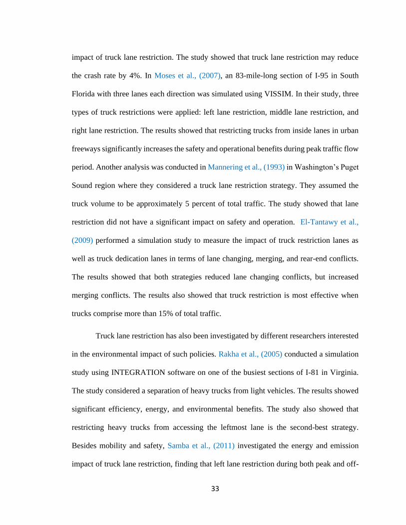
33
impact of truck lane restriction. The study showed that truck lane restriction may reduce
the crash rate by 4%. In Moses et al., (2007), an 83-mile-long section of I-95 in South
Florida with three lanes each direction was simulated using VISSIM. In their study, three
types of truck restrictions were applied: left lane restriction, middle lane restriction, and
right lane restriction. The results showed that restricting trucks from inside lanes in urban
freeways significantly increases the safety and operational benefits during peak traffic flow
period. Another analysis was conducted in Mannering et al., (1993) in Washington’s Puget
Sound region where they considered a truck lane restriction strategy. They assumed the
truck volume to be approximately 5 percent of total traffic. The study showed that lane
restriction did not have a significant impact on safety and operation. El-Tantawy et al.,
(2009) performed a simulation study to measure the impact of truck restriction lanes as
well as truck dedication lanes in terms of lane changing, merging, and rear-end conflicts.
The results showed that both strategies reduced lane changing conflicts, but increased
merging conflicts. The results also showed that truck restriction is most effective when
trucks comprise more than 15% of total traffic.
Truck lane restriction has also been investigated by different researchers interested
in the environmental impact of such policies. Rakha et al., (2005) conducted a simulation
study using INTEGRATION software on one of the busiest sections of I-81 in Virginia.
The study considered a separation of heavy trucks from light vehicles. The results showed
significant efficiency, energy, and environmental benefits. The study also showed that
restricting heavy trucks from accessing the leftmost lane is the second-best strategy.
Besides mobility and safety, Samba et al., (2011) investigated the energy and emission
impact of truck lane restriction, finding that left lane restriction during both peak and off-

34
peak times is a very effective strategy in terms of both mobility and safety. The simulation
study also showed that left lane restriction would decrease likelihood of crashes, especially
those involving heavy trucks. The study also showed that left lane restriction reduced fuel
consumption by 4% but increased CO2 emissions by 1.7%.
Second, route restriction refers to restricting trucks from accessing certain
highways and/or roads. This is often done in urban areas, especially in highly populated
areas. Truck lane restriction exists in most states in the U.S., particularly New York,
Virginia, and California. For example, truck route restrictions exist in the Ventura Freeway
in Los Angeles, CA and all roads going through downtown Atlanta, GA (Fitzpatrick et al.,
1992). In New York, truck route restrictions exist in many different sections of the state’s
freeways, such as I-81 from Exit 8 to NY 13A, I-81 from Exit 12 to US 20, NY 89 to NY
414, NY 90 to NY 34, and others (NYSDOT, n.d.). In Virginia, truck route restrictions
exist in many different parts of the state as seen in Figure 2-2 (VDOT, n.d.). In the city of
Cambridge, Massachusetts, truck routes restrictions have already been implemented on
several routes within the city (see Figure 2-3) (City of Cambridge, n.d.).
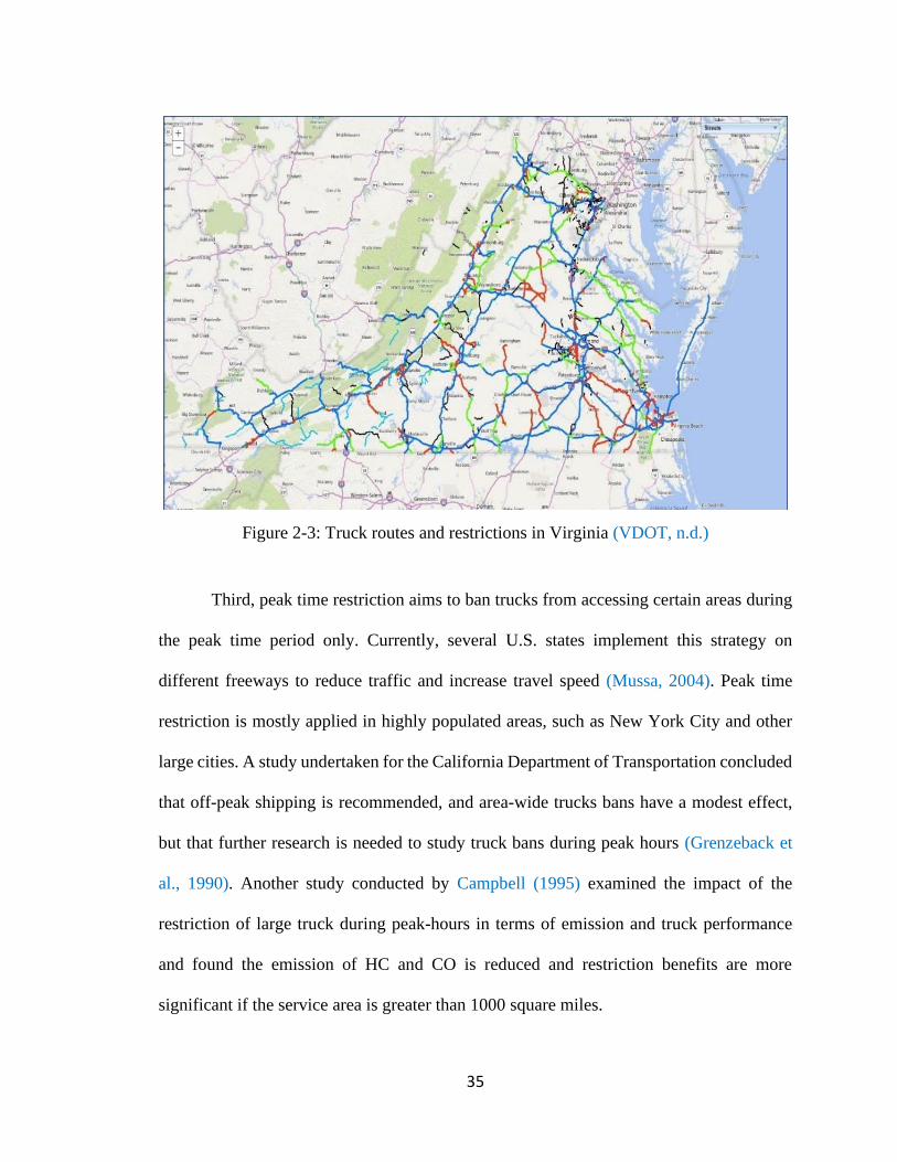
35
Figure 2-3: Truck routes and restrictions in Virginia (VDOT, n.d.)
Third, peak time restriction aims to ban trucks from accessing certain areas during
the peak time period only. Currently, several U.S. states implement this strategy on
different freeways to reduce traffic and increase travel speed (Mussa, 2004). Peak time
restriction is mostly applied in highly populated areas, such as New York City and other
large cities. A study undertaken for the California Department of Transportation concluded
that off-peak shipping is recommended, and area-wide trucks bans have a modest effect,
but that further research is needed to study truck bans during peak hours (Grenzeback et
al., 1990). Another study conducted by Campbell (1995) examined the impact of the
restriction of large truck during peak-hours in terms of emission and truck performance
and found the emission of HC and CO is reduced and restriction benefits are more
significant if the service area is greater than 1000 square miles.
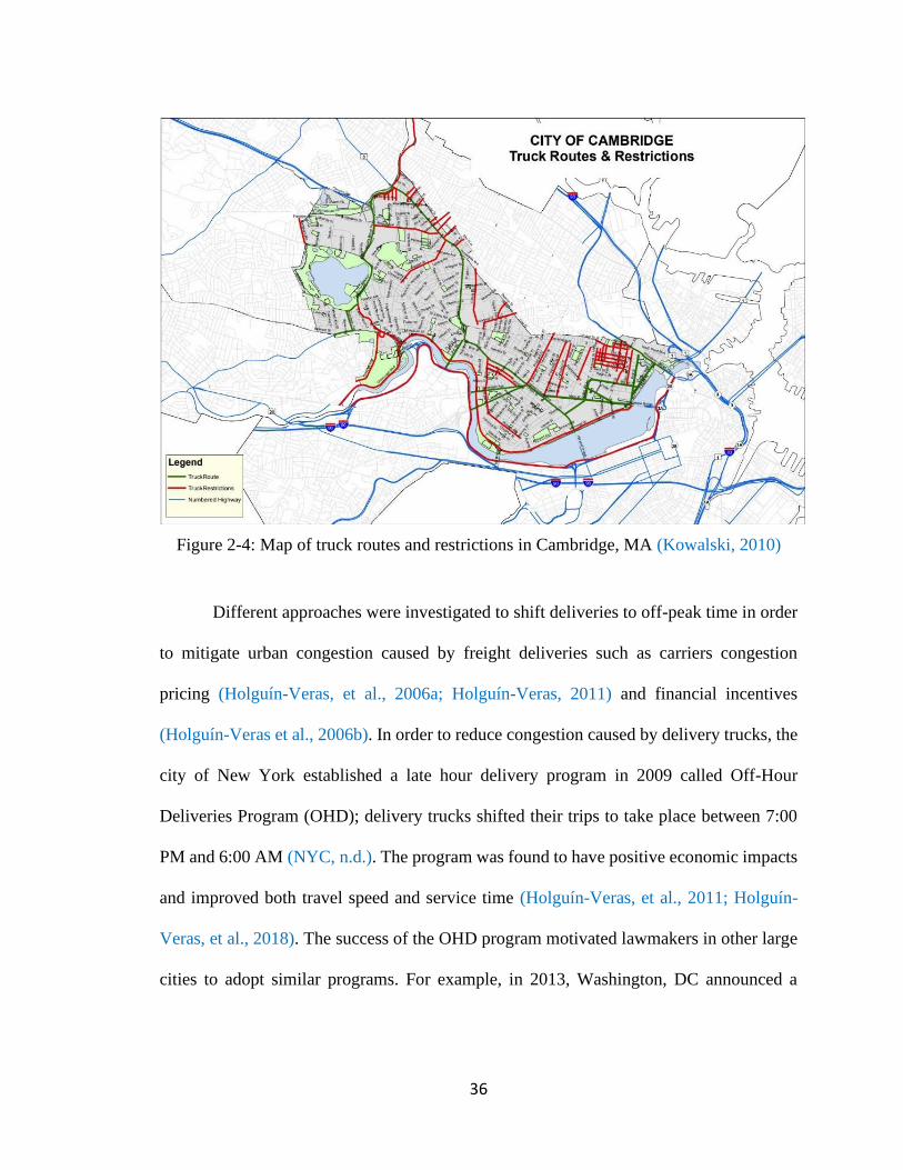
36
Figure 2-4: Map of truck routes and restrictions in Cambridge, MA (Kowalski, 2010)
Different approaches were investigated to shift deliveries to off-peak time in order
to mitigate urban congestion caused by freight deliveries such as carriers congestion
pricing (Holguín-Veras, et al., 2006a; Holguín-Veras, 2011) and financial incentives
(Holguín-Veras et al., 2006b). In order to reduce congestion caused by delivery trucks, the
city of New York established a late hour delivery program in 2009 called Off-Hour
Deliveries Program (OHD); delivery trucks shifted their trips to take place between 7:00
PM and 6:00 AM (NYC, n.d.). The program was found to have positive economic impacts
and improved both travel speed and service time (Holguín-Veras, et al., 2011; Holguín-
Veras, et al., 2018). The success of the OHD program motivated lawmakers in other large
cities to adopt similar programs. For example, in 2013, Washington, DC announced a

37
similar program which they called the Off-hours Freight Delivery Project which launched
in spring 2015 (DDOT , 2013).
Fourth, speed restriction refers to where trucks are assigned a lower speed than
passenger vehicles. Currently, fifteen states have adopted this law (U.S. DOT, 2012). In
2016, the U.S. Department of Transportation announced that the Department’s NHTSA
and Federal Motor Carrier Safety Administration (FMCSA) are proposing a new safety
measure which requires trucks weighing more than 26,000 pounds to be equipped with
devices limiting their speed (FMCSA, 2016). However, Wilmot & Khanal (1999)
conducted a review to examine whether speed limit reduction resulted in safety
enhancement and found that a differential speed limit among cars and trucks does not
enhance road safety.
2-5-2. Road Space Rationing-Based Restriction
Passenger vehicles are also exposed to restriction in many cases. In crowded areas,
such as Beijing, China or Delhi, India, vehicle restriction has become necessary to maintain
both normal traffic conditions and acceptable air quality. One popular restriction strategy
is based on the license plate number. This strategy is called Road Space Rationing and it
aims to divide all vehicles into two or more groups based on the last digit of their license
plate number.
(1) China’s Case Study
When China hosted the Olympic Games in August 2008, the Chinese government
needed to reduce the amount of traffic on the roads significantly. The restriction was
applied in different phases from July 1 to September 20, 2008 as shown in Table 2-2. The
goal of this strategy was to encourage drivers to change their travel mode and switch to

38
public transportation to reduce air pollution and to also improve air quality. During the
Olympics phase (July, 20 – September, 20) it was estimated that about 45 percent of the
total vehicles within the 5th ring area (the blue highway in Figure 2-4) were off of the streets
which prompted further investigation of the long-term impact (Wang et al., 2010; Han et
al., 2010) and the public acceptance and perception of this scheme (Jia et al., 2017).
Table 2-2: The phases of road space rationing implementation in Beijing (Li & Guo, 2016)
Phase Period Duration Method
Trial Aug. 17 – 20,
2007 6:00 AM -
Midnight Trial implementation within entire Beijing
1 July 1 – 19,
2008 3:00 AM -
Midnight High emission vehicles (yellow label vehicles) are
banned. Entire Beijing
2 July 20 – Aug.
27, 2008 3:00 AM -
Midnight Traffic restriction within the city administrative
areas. Entire Beijing
3 Aug. 28 –
Sept. 20, 2008 3:00 AM -
Midnight Restriction was limited to the road network within the
5th ring area.
2-3 July 20 – Sept.
20, 2008 3:00 AM -
Midnight
Olympics lane network were created for specific cars
which reduced 70% of government cars and 50% of
private cars in total of 20 million vehicles.

39
Figure 2-5: Map of major ring highways in Beijing, China
After September 20, 2008, the Beijing lawmakers announced a new restriction
strategy called the “one day a week scheme” to be enforced starting on October 11, 2008
(see Table 2-3). Therefore, it implemented a traffic restriction strategy which separated the
vehicles into two groups based on their license plate numbers. Vehicles which carried even
or odd license plate numbers and were each allowed to drive during certain days of the
week. The strategy aimed to further improve traffic mobility and air quality. They
estimated that 930,000 vehicles were banned, almost 26% of the total 3.6 million vehicles
in the region (Dingding, 2009).

40
Table 2-3: The one day a week driving scheme timeline (Wang et al., 2014)
Period Restriction time Restriction area Violation
penalty Rotation
period
Oct, 11, 2008 – Apr. 10,
2009 6:00 AM – 9:00 PM Within 5th ring
$15.8
daily Monthly
Apr. 5, 2009 – Jan. 8, 2012 7:00 AM – 8:00 PM Within 5th ring $15.8
daily Every13
Weeks
Jan. 9, 2012 – now 7:00 AM – 8:00 PM Within 5th ring $15.8
daily Every13
Weeks
The rotation process consisted of five groups based on the last digit of the license
plate (1&6, 2&7, 3&8, 4&9, and 5&0). If the last character is letter, then it was assumed
to be zero (Beijing Municipal People's Government, 2017). Each group was assigned to a
specific day of a week (Monday – Friday) for 13 weeks. Over the next 13 weeks, each
group was assigned to a different day. Table 2-4 below is an example of the current 2017
– 2018 rotation schedule:
Table 2-4: The 2017-18 rotation schedule based on last digit of license plate (Beijing
Municipal People's Government, 2017)
Rotation Schedule Monday Tuesday Wednesday Thursday Friday
April 10, 2017-July 9, 2017 3 & 8 4 & 9 5 & 0 1 & 6 2 & 7
July 10, 2017-Oct. 8, 2017 2 & 7 3 & 8 4 & 9 5 & 0 1 & 6
Oct. 9, 2017-Jan. 7, 2018 1 & 6 2 & 7 3 & 8 4 & 9 5 & 0
Jan. 8, 2018-April 8, 2018 5 & 0 1 & 6 2 & 7 3 & 8 4 & 9
(2) India’s Case Study
From 2011-2015, the megacity of Delhi, India was ranked as the most polluted city
in the world in terms of particle pollution (PM10 and PM2.5) by the World Health

41
Organization (WHO, 2016). Consequently, as an emergency action, the government in
Delhi, India implemented an odd-even traffic restriction from January 1st – 15th, 2016 and
April 15th – 30th, 2016 between 8:00 AM – 8:00 PM Monday-Saturday such that vehicles
with plate numbers ending with an odd number were restricted from driving on even dates
and vice versa (Delhi Transport Department, 2015). The government also banned other
types of vehicles, such as older diesel vehicles, from being operated inside the city of Delhi.
As an attempt to evaluate the environmental impact of this odd-even restriction in Delhi,
(Kumar et al., 2017) measured the level of PM10 and PM2.5 during the odd-even
implementation period (1-15, JAN 2016, 15-30, APR 2016) in different areas of Delhi and
compared this with data from the previous year during same period. The results showed
that the scheme reduced both PM10 and PM2.5 by up to 74 percent during peak hours, but
also increased their levels during the early morning hours due to overnight heavy vehicle
operations. Another experimental study was conducted by Chowdhury, et al. (2017) to
measure the level of PM2.5 during the odd-even implementation period (1-15, JAN 2016)
and found that the odd-even policy reduced the PM2.5 levels by 4-6 percent in three
different hotspots, which is not significant considering this was an emergency action.
Similarly, Jain, Gupta, & Ahuja (2016) conducted a four-day experimental study where
they chose three different time intervals to measure the air quality during morning rush
hour (8-10 AM), sleeping hours (1-3 PM), and evening rush hours (6-8 PM). The four days
included an odd day, even day, a Sunday, and a non-odd-even day. The result concluded
that during the scheme, the air quality was worse as compared to the non-odd-even days.
However, a 3-week landfill fire occurred during the experiment, which could have
impacted the results. In their experiment, by comparing the first week of the scheme

42
(January 1-7, 2016) to the week before (December 25-31, 2015) Sehgal & Gautam (2016)
concluded that the odd-even scheme experienced a significant increase in the PM
concentration, with the average PM level increasing from 148.7 μg m−3 to 241.4 μg m−3. In
addition to its impact on air quality, Mohan et al. (2017) conducted an observational
experiment in 4 different locations in Delhi and concluded that odd-even restriction
reduced traffic flow by more than 20%, but had no impact on reducing the PM2.5 levels.
During the first odd-even implementation period (1-15, JAN 2016) in Delhi, (Rao et al.,
2017) conducted an experiment to measure its impact on traffic congestion. Their results
showed that after the odd-even policy car speed was reduced up to 16 percent and travel
time increased by up to 20 percent. Their results also showed that the policy increased
demand for public transportation by up to 18%.
2-6. Credit-Based Restriction
The increasing number of vehicles in urban areas has played a major role in
worsening congestion and increasing emission levels. To curb this trend, researchers have
proposed a new credit-based traffic restriction (CBTR) policy which aims to reduce the
average miles traveled within a network to help reduce both congestion and emission.
CBTR policies are inspired by the cap-and-trade program proposed by (Crocker, 1966;
Dales, 1968a, 1968b) as a way to tackle air and water pollution. Cap-and-trade programs
are based on Coase (1960) who suggested that factories should be liable for the emission
harms they cause to others. A growing body of literature has intensively reviewed cap-and-
trade programs (Tietenberg, 2003; Paltsev, et al., 2008; Carl & Fedor, 2016). Cap-and-
trade (also known as tradable credit/permit) programs aim to help maintain a healthy
environment and limit the level of carbon emitted in the air by generally following two
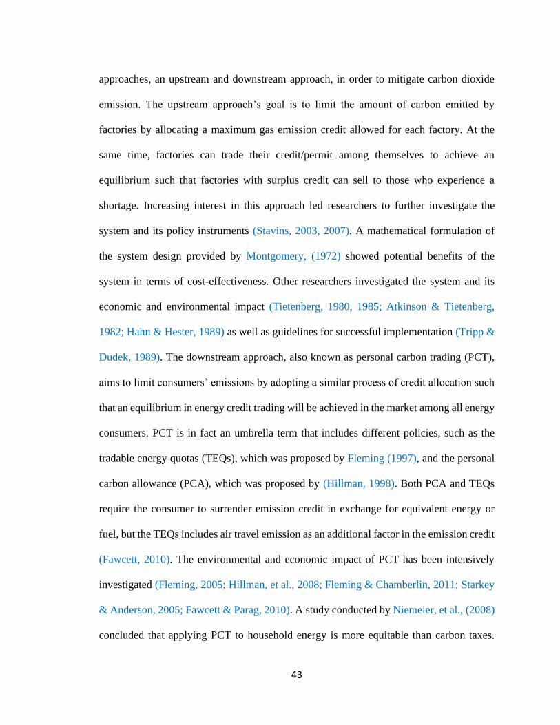
43
approaches, an upstream and downstream approach, in order to mitigate carbon dioxide
emission. The upstream approach’s goal is to limit the amount of carbon emitted by
factories by allocating a maximum gas emission credit allowed for each factory. At the
same time, factories can trade their credit/permit among themselves to achieve an
equilibrium such that factories with surplus credit can sell to those who experience a
shortage. Increasing interest in this approach led researchers to further investigate the
system and its policy instruments (Stavins, 2003, 2007). A mathematical formulation of
the system design provided by Montgomery, (1972) showed potential benefits of the
system in terms of cost-effectiveness. Other researchers investigated the system and its
economic and environmental impact (Tietenberg, 1980, 1985; Atkinson & Tietenberg,
1982; Hahn & Hester, 1989) as well as guidelines for successful implementation (Tripp &
Dudek, 1989). The downstream approach, also known as personal carbon trading (PCT),
aims to limit consumers’ emissions by adopting a similar process of credit allocation such
that an equilibrium in energy credit trading will be achieved in the market among all energy
consumers. PCT is in fact an umbrella term that includes different policies, such as the
tradable energy quotas (TEQs), which was proposed by Fleming (1997), and the personal
carbon allowance (PCA), which was proposed by (Hillman, 1998). Both PCA and TEQs
require the consumer to surrender emission credit in exchange for equivalent energy or
fuel, but the TEQs includes air travel emission as an additional factor in the emission credit
(Fawcett, 2010). The environmental and economic impact of PCT has been intensively
investigated (Fleming, 2005; Hillman, et al., 2008; Fleming & Chamberlin, 2011; Starkey
& Anderson, 2005; Fawcett & Parag, 2010). A study conducted by Niemeier, et al., (2008)
concluded that applying PCT to household energy is more equitable than carbon taxes.
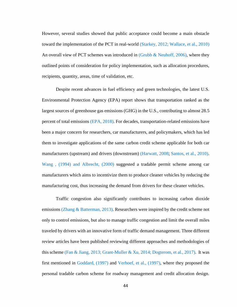
44
However, several studies showed that public acceptance could become a main obstacle
toward the implementation of the PCT in real-world (Starkey, 2012; Wallace, et al., 2010)
An overall view of PCT schemes was introduced in (Grubb & Neuhoff, 2006), where they
outlined points of consideration for policy implementation, such as allocation procedures,
recipients, quantity, areas, time of validation, etc.
Despite recent advances in fuel efficiency and green technologies, the latest U.S.
Environmental Protection Agency (EPA) report shows that transportation ranked as the
largest sources of greenhouse gas emissions (GHG) in the U.S., contributing to almost 28.5
percent of total emissions (EPA, 2018). For decades, transportation-related emissions have
been a major concern for researchers, car manufacturers, and policymakers, which has led
them to investigate applications of the same carbon credit scheme applicable for both car
manufacturers (upstream) and drivers (downstream) (Harwatt, 2008; Santos, et al., 2010).
Wang , (1994) and Albrecht, (2000) suggested a tradable permit scheme among car
manufacturers which aims to incentivize them to produce cleaner vehicles by reducing the
manufacturing cost, thus increasing the demand from drivers for these cleaner vehicles.
Traffic congestion also significantly contributes to increasing carbon dioxide
emissions (Zhang & Batterman, 2013). Researchers were inspired by the credit scheme not
only to control emissions, but also to manage traffic congestion and limit the overall miles
traveled by drivers with an innovative form of traffic demand management. Three different
review articles have been published reviewing different approaches and methodologies of
this scheme (Fan & Jiang, 2013; Grant-Muller & Xu, 2014; Dogterom, et al., 2017). It was
first mentioned in Goddard, (1997) and Verhoef, et al., (1997), where they proposed the
personal tradable carbon scheme for roadway management and credit allocation design.
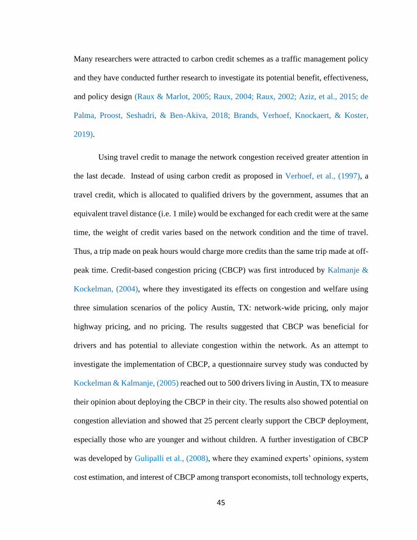
45
Many researchers were attracted to carbon credit schemes as a traffic management policy
and they have conducted further research to investigate its potential benefit, effectiveness,
and policy design (Raux & Marlot, 2005; Raux, 2004; Raux, 2002; Aziz, et al., 2015; de
Palma, Proost, Seshadri, & Ben-Akiva, 2018; Brands, Verhoef, Knockaert, & Koster,
2019).
Using travel credit to manage the network congestion received greater attention in
the last decade. Instead of using carbon credit as proposed in Verhoef, et al., (1997), a
travel credit, which is allocated to qualified drivers by the government, assumes that an
equivalent travel distance (i.e. 1 mile) would be exchanged for each credit were at the same
time, the weight of credit varies based on the network condition and the time of travel.
Thus, a trip made on peak hours would charge more credits than the same trip made at off-
peak time. Credit-based congestion pricing (CBCP) was first introduced by Kalmanje &
Kockelman, (2004), where they investigated its effects on congestion and welfare using
three simulation scenarios of the policy Austin, TX: network-wide pricing, only major
highway pricing, and no pricing. The results suggested that CBCP was beneficial for
drivers and has potential to alleviate congestion within the network. As an attempt to
investigate the implementation of CBCP, a questionnaire survey study was conducted by
Kockelman & Kalmanje, (2005) reached out to 500 drivers living in Austin, TX to measure
their opinion about deploying the CBCP in their city. The results also showed potential on
congestion alleviation and showed that 25 percent clearly support the CBCP deployment,
especially those who are younger and without children. A further investigation of CBCP
was developed by Gulipalli et al., (2008), where they examined experts’ opinions, system
cost estimation, and interest of CBCP among transport economists, toll technology experts,

46
administrators, and policy-makers. They also investigated other aspects of CBCP such as
credit allocation, revenue usage, system enforcement, and economic impact. A study that
predicts the impact of CBCP on traffic, air quality, welfare, and the cost of implementation
in the Dallas-Fort Worth metro area (DFW) was conducted by Gulipalli & Kockelman,
(2008) and found welfare improvement among the majority of drivers and predicted that a
high level of recurring congestion would practically disappear. Moreover, Kockelman &
Lemp, (2011) compared three different pricing policies in terms of revenue-generating:
flat-tolling schemes, standard congestion pricing, and CBCP. Recently, Liu & Nie, (2017),
investigated a Pareto-improving credit-based congestion management scheme. They
assumed a general two-mode network where transit is a cheaper, but slower alternative to
driving alone and they showed that a good transit coverage will generate positive net
revenue.
The diffusion of travel credit as a traffic management scheme encouraged
researchers to explore further extensions. Recently, the tradable credit scheme (TCS) has
gained momentum and was given great interest among researchers who conducted multiple
studies that investigate and compare tradable credit with current practices for its
effectiveness in improving congestion, environmental, and economic conditions (Crals,
2005; Crals & Vereeck, 2005; Raux, 2008). According to Grant-Muller & Xu, (2014),
researchers generally followed three different approaches to tackle the traffic congestion
using the tradable credit scheme: mobility management, bottleneck management, and
parking management. Among the many studies categorized into the first group, a
remarkable contribution was made by Yang & Wang, (2011) who proposed a mathematical
formulation framework of tradable mobility credit (TMC) scheme. They assumed

47
homogenous travelers in the network where the government initially allocated a certain
amount of credits to each eligible driver. Drivers then would be charged a specific amount
of credit as they travel on each link. At the same time, travelers can sell surplus or buy
shortage credits among themselves in a credit trading market. Their work has been carried
out to include different aspects, such as heterogeneous travelers (Wang et al., 2012; Zhu
et al., 2014 ); the impact of transaction cost on auction market, where travelers buy their
needed credits by bidding, and a negotiated market, where credits are initially allocated by
the government to drivers and they can trade with each other (Nie, 2012), income and
equity (Wu, et al., 2012; Wang, et al., 2014a); and “safety valve policy” which aims to
resolve the credit price volatility under demand uncertainty (Shirmohammadi, et al., 2013).
Considering both finite and infinite number of players, a variational inequality formulation
was formulated by (He, et al., 2013) to capture the impact of the transaction cost on the
tradable system and found that transaction cost impacted the trading volume when applied.
Wang & Yang, (2012) and Wang, et al., (2014b) proposed a modified bisection based
procedure for trial-and-error implementation of the tradable credit schemes on a single road
and general network respectively. Ye & Yang (2013) examined the day-to-day evolution
of credit price and traffic flow dynamics under TMC scheme considering travelers’
learning behavior. Miralinaghi & Peeta, (2016) proposed a multi-period tradable credit
scheme as an approach to alleviate credit price volatility. In a multi-period scheme, unused
credits could be transferred to future periods, either with or without penalty fees. The
findings of this study showed that multi-period schemes mitigate credit price volatility and
transfer fees have an advantage over free transfer by allowing the central authority to have
more control over credit hoarding.

48
In the second group, TCS as a system generally follows the same credit allocation
and trading process with some exceptions. The tradable bottleneck permit, also called
tradable bottleneck credits (TBC), aims to curb peak hour congestion by mitigating the
demand of selected critical bottlenecks within the network such that all drivers require a
permit/credit to access these specific bottlenecks. It was first proposed by Akamatsu et al.,
(2006), as “tradable bottleneck permits”, where they showed the efficiency of the scheme
to mitigate morning peak time congestion. Their model suggested that a limited number of
permits to access the bottleneck should be initially issued by the authority, and each permit
should be valid for a prespecified time period. At the same time, a trading market should
be founded to allow travelers to trade and obtain their permits. Xiao et al., (2013)
investigated the effectiveness and the efficiency of tradable credit scheme in managing
peak commute congestion. The results showed that combining initial credit allocation and
optimal credit charging can achieve SO and equality. Tian et al., (2013) examined the
efficiency of a tradable travel credit scheme in terms of bottleneck congestion. They
assumed heterogenous value of time (VOT) among drivers and allocated credits among
them. At the same time, drivers could trade credit in a virtual market. The results showed
that when SO is achieved, the optimal-credit scheme is always Pareto-improving. A new
TCS mechanism was proposed by Nie & Yin (2013) and Nie (2015) to manage critical
bottlenecks in the network such that driving credits will be charged to access critical
bottlenecks during peak time. Their proposed scheme suggested that instead of allocating
credits to drivers, travelers will be rewarded with credits by accessing bottlenecks during
off-peak times and can sell their credits to travelers who access these bottlenecks during
peak times. Their analysis indicated there would be up to 33 percent gain in efficiency and
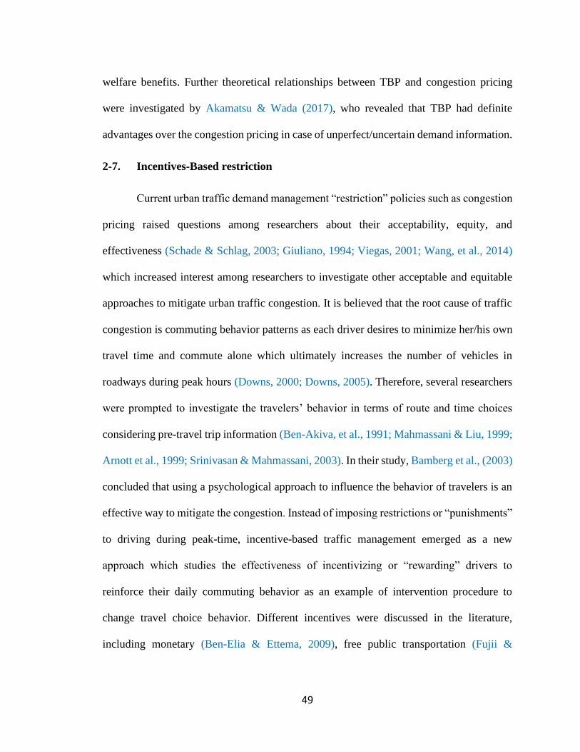
49
welfare benefits. Further theoretical relationships between TBP and congestion pricing
were investigated by Akamatsu & Wada (2017), who revealed that TBP had definite
advantages over the congestion pricing in case of unperfect/uncertain demand information.
2-7. Incentives-Based restriction
Current urban traffic demand management “restriction” policies such as congestion
pricing raised questions among researchers about their acceptability, equity, and
effectiveness (Schade & Schlag, 2003; Giuliano, 1994; Viegas, 2001; Wang, et al., 2014)
which increased interest among researchers to investigate other acceptable and equitable
approaches to mitigate urban traffic congestion. It is believed that the root cause of traffic
congestion is commuting behavior patterns as each driver desires to minimize her/his own
travel time and commute alone which ultimately increases the number of vehicles in
roadways during peak hours (Downs, 2000; Downs, 2005). Therefore, several researchers
were prompted to investigate the travelers’ behavior in terms of route and time choices
considering pre-travel trip information (Ben-Akiva, et al., 1991; Mahmassani & Liu, 1999;
Arnott et al., 1999; Srinivasan & Mahmassani, 2003). In their study, Bamberg et al., (2003)
concluded that using a psychological approach to influence the behavior of travelers is an
effective way to mitigate the congestion. Instead of imposing restrictions or “punishments”
to driving during peak-time, incentive-based traffic management emerged as a new
approach which studies the effectiveness of incentivizing or “rewarding” drivers to
reinforce their daily commuting behavior as an example of intervention procedure to
change travel choice behavior. Different incentives were discussed in the literature,
including monetary (Ben-Elia & Ettema, 2009), free public transportation (Fujii &

50
Kitamura, 2003) or discounted tolls (Bae & Bassok, 2008). The main objective of the
incentive is to encourage travelers to switch their travel mode or time.
An attempt to design a financial reward mechanism was introduced by Maillé &
Stier-Moses, 2009, where they developed an algorithm to determine the optimal monetary
reward for each commuting mode. The results show that rewards had a significant impact
on reducing commuting time and costs, especially in highly congested area.
Incentive-based traffic management first surfaced with the Spitsmijden1 (or Peak
Avoidance in Dutch) experiment in Zoetermeer, the Netherlands, which was conducted in
four phases between October 2006 and May 2009 (see Figure 2-5). In exchange for a
change in mode, route, or time change in their daily commute in morning peak hours, as
defined for each experiment, drivers were given a monetary incentive ranging from 2-7
Euros or credits to obtain a smartphone by the end of the experiment (see Table 2-5)
(Ettema & Verhoef, 2006; Knockaert, et al., 2007; Donovan, 2010; Bliemer et al., 2010).
During the Spitsmijden experiment, multiple survey studies were conducted among
341 drivers who participated to compare the characteristics of those who would participate
in the experiment and those would not and what factors had the greatest impact on their
decision. The results suggested that working time flexibility and household duties appeared
to be main factors to participate (Ben-Elia & Ettema, 2009; Ettema et al., 2010; Knockaert
et al., 2011). Although the result from Zoetermeer experiment suggest that incentives have
a great potential to mitigate congestion in the short run, it remains unclear if the changed
behavior will continue without rewards (Ben-Elia & Ettema, 2011a,b; Ben-Elia et al.,
1 “peak avoidance” in Dutch language
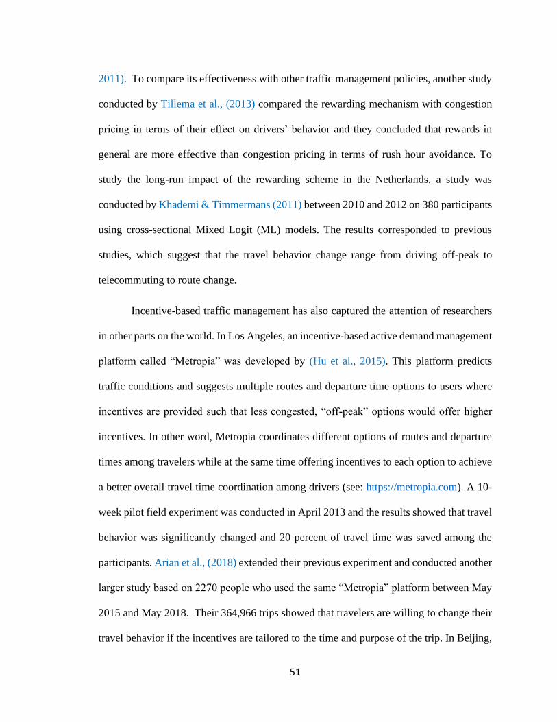
51
2011). To compare its effectiveness with other traffic management policies, another study
conducted by Tillema et al., (2013) compared the rewarding mechanism with congestion
pricing in terms of their effect on drivers’ behavior and they concluded that rewards in
general are more effective than congestion pricing in terms of rush hour avoidance. To
study the long-run impact of the rewarding scheme in the Netherlands, a study was
conducted by Khademi & Timmermans (2011) between 2010 and 2012 on 380 participants
using cross-sectional Mixed Logit (ML) models. The results corresponded to previous
studies, which suggest that the travel behavior change range from driving off-peak to
telecommuting to route change.
Incentive-based traffic management has also captured the attention of researchers
in other parts on the world. In Los Angeles, an incentive-based active demand management
platform called “Metropia” was developed by (Hu et al., 2015). This platform predicts
traffic conditions and suggests multiple routes and departure time options to users where
incentives are provided such that less congested, “off-peak” options would offer higher
incentives. In other word, Metropia coordinates different options of routes and departure
times among travelers while at the same time offering incentives to each option to achieve
a better overall travel time coordination among drivers (see: https://metropia.com). A 10-
week pilot field experiment was conducted in April 2013 and the results showed that travel
behavior was significantly changed and 20 percent of travel time was saved among the
participants. Arian et al., (2018) extended their previous experiment and conducted another
larger study based on 2270 people who used the same “Metropia” platform between May
2015 and May 2018. Their 364,966 trips showed that travelers are willing to change their
travel behavior if the incentives are tailored to the time and purpose of the trip. In Beijing,

52
China, a survey study was conducted by Zhang et al., (2014) to investigate the impact of
incentives on commuters’ travel behavior within the Beijing subway system. Their results
showed that offering incentives such as coupons for food or free internet or discounted
ticket fare had a positive impact on changing the commuters travel time. The potential of
incentive-based traffic management has also encouraged the policymakers in congested
cities in the U.S. to implement this policy. For example, in Washington, DC, a carpooling
project to encourage lone drivers to carpool offered riders $1 for each way ($2 round trip)
per day if they carpooled to work. Success was achieved after the program ends where 93
percent of participants continued to carpool after the reward ended (icommute, 2012).
Figure 2-6: The four phases of Spitsmijden project in the Netherlands

53
Table 2-5: Summary of the Spitsmijden experiment (Donovan, 2010; Bliemer et al.,
2010)
Experiments
location
Timeline
Peak hour
Participants
Incentive
Behavior change
Zoetermeer
Oct.-Dec. 2006
7:30– 9:30 AM
340
3 Euros 46%
7 Euros 61%
Hollandse
Brug
Sept. 2007 Oct.
2008
6:00–10:00 AM
2,800
4 Euros
40%
Gouda Sept. 2008 -
May 2009
6:30– 9:30 AM
771
4 Euros
52%
Moerdijk
Brug
Apr. to Jul.
2008
3:00– 7:00 PM
2,703
4 Euros
54%
2-8. Conclusion
While several TDM strategies have been discussed in this chapter, SLEM could be seen to
share several similarities with the proposed TDM policies. As shown in Figure 2-7, SLEM
shares similarities with the financial-based restriction, namely the congestion pricing, by
imposing score restriction instead of monetary restriction. SLEM also shares similarities
with the credit-based TDM by limiting some drivers’ route choice during peak hours. In
addition, SLEM shares a similar approach as a categorization-based restriction, namely
road rationing, by incentivizing a portion of the drivers to change their commuting mode.
Additionally, SLEM is also an incentive-based restriction since it is motivating drivers to
improve their driving behavior through providing incentives. Similar to the performance-
based strategy, SLEM also uses real-time telematics data to monitor drivers and their
driving performance. Finally, SLEM could also be viewed as a priority-based TDM, such
as managed lanes, as it prioritizes safer drivers instead of high-occupancy and/or high-
income drivers.

54
Figure 2-7: SLEM similarities with other TDM strategies
2-9. Summary
This chapter reviewed the literature on different approaches used for driver style
profiling and monitoring as well as the history of the traffic demand management and
different restriction policies that have been proposed and implemented. The chapter
reviewed driving profiling approaches that have been discussed in the literature.
Researchers have mainly focused on detecting the driving style and the focus state of each
driver. Different approaches including pedal operation monitoring, have been used, and as
technology improved, more practical methods such as smartphones applications were used.
Driving performance profiling is a well-known method among automobile insurance
companies. Many insurance companies offer UBI policies where the driver provides the
company access to her/his driving data in a return for discounted policy rate. Furthermore,

55
the chapter also reviewed the numerous traffic restriction schemes that have been proposed
in the literature in the last five decades. Different approaches to tackle congestion,
including monetary penalties, vehicle occupancy increases, and travel mile limitations,
have been proposed.

56
Chapter 3
SURVEY DESIGN AND IMPLEMENTATION
3-1. Introduction
This chapter presents the survey design and its distribution procedure. A detailed
explanation of the survey design, participant recruitment, and distribution is provided in
this chapter. This chapter is divided into five sections. Section 3-2 presents an overview of
the survey structure. Section 3-3 summarizes the demographic data of the obtained sample
and compares this data to the population to ensure that the collected sample adequately
represents the population. Section 3-4 examines the quality of the data and its internal
consistency to measure its reliability. Finally, Section 3-5 summarizes the survey design
and implementation procedure.
3-2. Overview
A 32-question online survey was designed (See Appendix A) using Qualtrics
software to measure public opinion about SLEM (see https://www.qualtrics.com). The
survey was divided into three sections. The first section asked participants about their
driving habits, such as their daily commuting distance, mode of commute, and whether
they had had previous accidents and/or violations. The second section collected
information on the participants’ opinion about SLEM and their main reasons for supporting
or rejecting the system. The final section asked the participants for their demographic
information, including their current city of residence, age, and level of income. As a part

57
of the survey validation, the first draft of the survey was piloted in September 2017 with
twenty people from different backgrounds, majors, education levels, and nationalities at
our home institution of Southern Methodist University (SMU) to evaluate the overall
quality of the survey including time, flow, and clarity. Based on the pilot study, a short
animation video clip was provided to explain the overall concept of a SLEM system to
guarantee the consistency of the idea explanation, and to ensure equal understanding the
idea among participants, thereby enhancing data accuracy and reducing bias.2 A snapshot
of this video clip is provided in Figure 3-1. All survey participants were asked to watch the
video before starting the second section of the survey. This video ensured that every
participant received exactly the same information about the proposed system, thereby
enhancing data accuracy and reducing bias. The final revised form of the survey was
deemed exempt from review by SMU’s Institutional Review Board (IRB) and was
deployed on Mar 1st, 2018.
2 Video link
58
Vehicle Connectivity Driver Performance Scoring
Penalizing Violating Drivers Roadway Access Based on Score Value
Figure 3-1: Snapshots of the video used to demonstrate SLEM for the survey participants
The survey was distributed from March 1st to April 30th, 2018. Three approaches
were used to recruit a representative sample. First, to enlist recruiters, 45 students from
three different engineering classes (two undergraduate and one graduate) were invited to
participate voluntarily in the recruitment process; 32 students volunteered to participate as
recruiters. They recruited 376 valid participants from family members and their network
of friends who live in different states (an average of about 12 recruits per student). The
second approach was to recruit participants face-to-face in public places such as coffee
shops and shopping malls. These participants were asked to complete the survey either on
the spot using a tablet, or alternatively, they were emailed or texted the survey link so they
could complete the survey at their convenience. Those participants were also asked to share
the survey with their relatives and friends living in other states, if possible. This approach

59
produced 97 valid responses. The third approach used an academic, research-based online
crowdsourcing platform (see https://prolific.ac), widely used as reliable methods for data
collection (Rand et al., 2012). Previous researchers evaluated the reliability of these
platforms by comparing their data with data collected using other traditional approaches,
such as laboratory experiments and face-to-face interviews. They concluded that online
crowdsourcing platforms generally produce results indistinguishable from other methods
(e.g., Palan & Schitter, 2018). Through the online crowdsourcing platform used in this
study, a total of 1,009 participants were recruited from across the country, yielding 945
valid data points.
Figure 3-2: Geocode locations of participants (in orange) across all 50 states (N = 1418)
60
3-3. Initial Survey Data
The result produced a convenience sample of 1,672 participants, which satisfied the
minimum sample size requirements, following the methodology proposed in Krejcie &
Morgan (1970). Participants responded from all 50 states and from the District of Columbia
(DC). Eligible participants were U.S. residents who held a driver license (DL) during the
last 3 years. Data were cleaned by removing duplicate, inconsistent, careless, and
incomplete responses. The 1,672 total responses were reduced to a total of 1,418 valid
responses, which still covered all 50 states and the DC area, as presented in Figure 3-2.
Table 3-1 compares the sample with the U.S. population distribution for main demographic
variables. 49.3 percent (n = 700) of the participants were female, 50 percent (n = 708) were
male, and 0.7 percent (n = 10) of the participants identified themselves as another gender.
Participants were aged 16 years or older, with an average age of 37.2 years. The age
distribution of the sample slightly shifted towards younger age groups. The sample had a
larger proportion of drivers aged 25-39 (47.2 percent) than the corresponding value in the
U.S. population (20.3 percent). The sample also underrepresented drivers aged 60 or
greater (6.5 percent) compared to the population value (21.3 percent) (U.S. Census Bureau,
2017a; U.S. Census Bureau, 2018).
61
Participants were divided among five different race/ethnic groups: White (77.5
percent), Black or African American (4.5 percent), American Indian or Alaska Native (0.4
percent), Asian (8.8 percent), and another race or ethnicity (8.8 percent). The racial/ethnic
sample matched the U.S. population closely, with the exception of the Black/African
American sub-population and other race/ethnicity, where the sample proportion was
smaller. Finally, the distribution of household incomes in the sample generally matched
that of the population (U.S. Census Bureau, 2017b). Since enough data points were
collected for each sub-population category as per Krejcie & Morgan (1970), it was
concluded that the data were adequate for the purpose of the analysis conducted in this
dissertation.
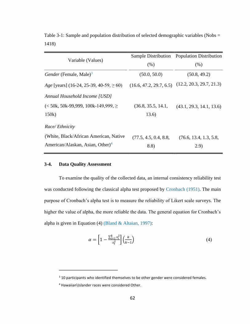
62
Table 3-1: Sample and population distribution of selected demographic variables (Nobs =
1418)
3-4. Data Quality Assessment
To examine the quality of the collected data, an internal consistency reliability test
was conducted following the classical alpha test proposed by Cronbach (1951). The main
purpose of Cronbach’s alpha test is to measure the reliability of Likert scale surveys. The
higher the value of alpha, the more reliable the data. The general equation for Cronbach’s
alpha is given in Equation (4) (Bland & Altaian, 1997):
𝛼 = [1 −∑ 𝑠𝑖
2𝑘𝑖=1
𝑠𝑡2 ] (
𝑘
𝑘−1) (4)
3 10 participants who identified themselves to be other gender were considered females.
4 Hawaiian\Islander races were considered Other.
Variable (Values) Sample Distribution
(%) Population Distribution
(%)
Gender (Female, Male)3 (50.0, 50.0) (50.8, 49.2)
Age [years] (16-24, 25-39, 40-59, ≥ 60) (16.6, 47.2, 29.7, 6.5) (12.2, 20.3, 29.7, 21.3)
Annual Household Income [USD]
(< 50k, 50k-99,999, 100k-149,999, ≥
150k)
(36.8, 35.5, 14.1,
13.6)
(43.1, 29.3, 14.1, 13.6)
Race/ Ethnicity
(White, Black/African American, Native
American/Alaskan, Asian, Other)4
(77.5, 4.5, 0.4, 8.8,
8.8)
(76.6, 13.4, 1.3, 5.8,
2.9)
63
where k is the number of items, 𝑠𝑖2 is the variance of the ith item, and 𝑠𝑡
2 is the
variance of the total score obtained by summing all items. A Cronbach’s alpha score that
is equal to 0.77 was obtained for the survey. According to Bland and Altaian (1997), a
survey with satisfactory internal reliability should have a Cronbach’s alpha score of 0.70
or above.
The second survey focused on obtaining experts’ perspectives of SLEM. Another
short questionnaire was designed using the Qualtrics software to target professionals in the
area of traffic operations, ITS, and safety. The survey included questions soliciting
information on the expert’s position, level of support for SLEM, and views about the
effectiveness of SLEM at enhancing traffic safety and alleviating traffic congestion.
Experts were also asked to list main obstacles that may prevent the adoption of this new
technology in their regions. Finally, they were asked whether public agencies or private
companies should operate such a system. The survey was distributed by email to more than
100 professionals who were identified from web-based professional networks (e.g.,
LinkedIn) and by visiting the websites of public agencies and consulting firms. Twenty
responses were obtained from 10 different states covering 16 different cities. Participants
mostly worked as senior traffic operations and safety engineers with expertise in ITS.
3-5. Summary
This chapter summarized data obtained by the survey to assure its quality and
reliability. First, the representativeness of the data was tested compared to the national
population in terms of several demographics. The results showed a high rate of
representativeness in most demographic variables, with a few biases and

64
underrepresentation for some groups. Second, a Cronbach’s alpha test evaluated the data’s
internal consistency and reliability. A Cronbach's alpha of 0.77 indicated significant
internal consistency and thus, the data had overall significant reliability.
65
Chapter 4
SURVEY RESULTS AND ANALYSIS
4-1. Introduction
This chapter presents the results of the two distributed surveys. First, the chapter
describes the public opinion survey discussed in the previous chapters. This survey
revealed participants’ driving characteristics, their driving routines, and their willingness
to change their daily driving habits. This chapter also presents their perception of SLEM
including reporting and discussing reasons for rejection or acceptance of SLEM. A logistic
regression of results, where the main characteristics of those who accept/reject the
implementation of SLEM was discussed, is presented. Second, the results from another
survey which targeted transportation experts is also presented here. Experts were asked
about their opinion of SLEM and why they would support or reject its implementation.
Third, different future scenarios were modeled based on a logistic regression model where
different variables were considered to measure the effect of each on public acceptance.
This chapter is divided into eight sections. An overview of the demographic and driving
characteristics of the participants are provided in sections 4-2 and 4-3, respectively. In
section 4-4, a detailed public perception of SLEM is given followed by the expert
perception of SLEM in section 4-5. Section 4-6 provides the survey analysis results in the
form of a logistic regression where different models were developed. Finally, the effects

66
on SLEM implementation and the issues associated with its real-world deployment
are given in sections 4-7 and 4-8, respectively.
4-2. Demographic Characteristics
The baseline data obtained from the first survey were first analyzed using
preliminary descriptive statistics. Table 4-1 provides a summary of participants’
demographic information. Most participants (54.5 percent) reported themselves as married
or in a domestic relationship. In addition, about 45.5 percent of participants had at least
one child. 37.5 percent of the participants reported a bachelor’s degree as their highest level
of education. Other participants reported their highest education to be some college (27.5
percent), a master’s degree (22.4 percent), a doctoral degree (6.6 percent), or high school
or less (5.9 percent). Respondents were mostly employed, either full- or part-time (57.7
and 17.5 percent, respectively). Ten percent were students, and only 7.9 percent reported
being unemployed. Among the 1,418 respondents, 69.5 percent lived in urban areas. The
highest number of participants were from Texas (181 participants), California (169
participants), and New York (99 participants), respectively.

67
Table 4-1: Summary of the demographics data of the survey participants
4-3. Driving Characteristics
Table 4-2 includes a summary of the participants’ commuting experience. About
35.5 percent of participants defined themselves as experienced drivers with more than 20
years of driving. In addition, 61.1 percent of the participants commuted 5 days or more
weekly, and 80.7 percent of them commuted less than 25 miles daily. About 81.5 percent
of the participants commuted alone, and only 4.9 percent carpooled. Almost one-third of
the participants (32.7 percent) had one or more tickets in the last 5 years, and 32 percent
also experienced at least one car accident during the same time period. In addition, 13.7
percent of individuals reported that they had points on their driver licenses. Speeding was
reported as the most common ticket received by drivers (42.3 percent). Running a red light
was the second most common traffic violation (7.3 percent). Figure 4-1 shows a summary
of different violations reported by participants.
Variable Percentage (%)
Marital Status (Married, Single, Divorced, Widowed,
Separated)
(54.5, 38.8, 4.9, 0.9, 0.9)
Number of Children (None, 1, 2, 3, > 3 Children) (54.5, 15.5, 18.3, 7.7, 4.0)
Education (No High School, High School Diploma,
Some College, Bachelor’s, Master’s, Doctoral)
(0.2, 5.8, 27.5, 37.5, 22.4,
6.6)
Employment (Full-Time, Part-Time, Student,
Unemployed, Retired, Disabled, Other)
(57.7, 17.5, 10.1, 7.9, 3.4,
0.7, 2.7)
Urbanization (Yes, No) (69.5, 30.5)

68
Figure 4-1: Reported traffic violations
Table 4-2: Summary of the commute characteristics data of the survey participants
Table 4-3 summarizes the participants’ perception of congestion and their attitudes
toward different actions to reduce traffic congestion. The majority (72.2 percent) of
Variable Percentage (%)
Driving Experience [years] (< 4, 4-10, 11-20, > 20) (8.5, 29.5, 26.5, 35.5)
Weekly Commuting [days] (0, 1, 2, 3, 4, 5, > 5) (11.5, 2.8, 5.5, 10.4, 8.8, 39.4,
21.6) Commute Distance [miles] (< 5, 5-9, 10-14, 15-24,
25-39, 40-59, 60-79, > 80)
(22.0, 19.1, 19.5, 20.0, 11.0, 4.8,
1.8, 1.8)
5-Years, Accidents (0, 1, 2, 3, > 3) (67.3, 23.2, 6.8, 1.8, 0.9)
5-Years, Tickets (0, 1, 2, 3, > 3) (68.0, 21.6, 6.5, 2.7, 1.2)
Commute Mode
(Drive Alone, Public Transportation, Carpool,
Other)
(81.5, 6.6, 4.9, 7.0)
Points on DL (No, Yes) (86.3, 13.7)
Type of Ticket
(Speeding, Running a Red Light, Running a
Stop Sign, Wrong Parking, Speeding & Running a
Red Light, Other)
(42.3, 7.2, 4.0, 3.0, 3.3, 40.2)

69
individuals agreed that congestion is a daily commute problem they face, and about 70.8
percent of them were willing to change their commuting routine to avoid this congestion.
Changing their route is the most common action by individuals to avoid congestion (85.3
percent).
Table 4-3: Summary of the congestion perception data of the survey participants
The second most common action considered by the survey participants is changing
the trip departure time (78.7 percent). Telecommuting is the third top action to avoid
congestion (55.7 percent). Changing the travel mode and carpooling are the least favored
Variable
Strongly
Disagree
(%)
Somewhat
Disagree
(%)
Neutral
(%)
Somewhat
Agree
(%)
Strongly
Agree
(%)
General View of Drivers’ Performance
Congestion is a Commute Problem 8.8 10.0 9.0 36.5 35.7
Support DL suspension as
Punishment 1.2 2.0 5.0 31.8 60.0
Willingness to Change Commuting
Routine 1.6 5.4 22.2 37.9 32.9
Action to Avoid Traffic Congestion
Change Time 4.3 10.9 6.1 43.6 35.1
Change Route 2.4 6.3 6.0 46.9 38.4
Change Mode 16.4 24.4 17.6 28.1 13.5
Carpool 20.4 25.7 16.2 27.3 10.4
Telecommuting 15.8 11.9 16.6 22.2 33.5
Do Nothing 19.4 16.9 37.4 17.4 8.8
Incentives to Motivate Changing Commute Performance
Insurance Discount 1.6 3.6 10.3 36.3 48.2
Express Lane Access 2.9 7.8 16.5 35.5 37.3
Free Discounted Parking 7.0 6.3 21.4 25.2 40.1
Free Discounted Tolls 5.6 5.9 21.4 27.0 40.1
Discounted DL Renewal 4.7 8.7 20.1 31.5 35.0
Monetary Reward 1.3 2.0 8.5 25.1 63.1
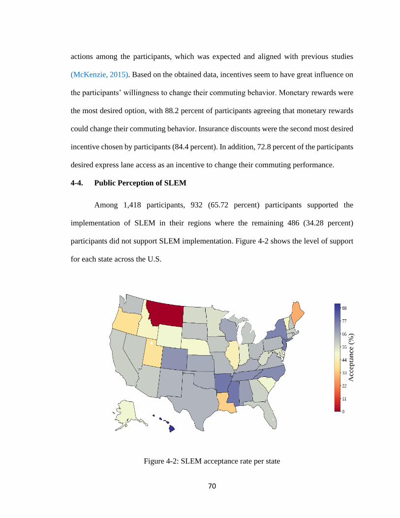
70
actions among the participants, which was expected and aligned with previous studies
(McKenzie, 2015). Based on the obtained data, incentives seem to have great influence on
the participants’ willingness to change their commuting behavior. Monetary rewards were
the most desired option, with 88.2 percent of participants agreeing that monetary rewards
could change their commuting behavior. Insurance discounts were the second most desired
incentive chosen by participants (84.4 percent). In addition, 72.8 percent of the participants
desired express lane access as an incentive to change their commuting performance.
4-4. Public Perception of SLEM
Among 1,418 participants, 932 (65.72 percent) participants supported the
implementation of SLEM in their regions where the remaining 486 (34.28 percent)
participants did not support SLEM implementation. Figure 4-2 shows the level of support
for each state across the U.S.
Figure 4-2: SLEM acceptance rate per state
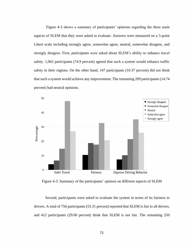
71
Figure 4-3 shows a summary of participants’ opinions regarding the three main
aspects of SLEM that they were asked to evaluate. Answers were measured on a 5-point
Likert scale including strongly agree, somewhat agree, neutral, somewhat disagree, and
strongly disagree. First, participants were asked about SLEM’s ability to enhance travel
safety. 1,062 participants (74.9 percent) agreed that such a system would enhance traffic
safety in their regions. On the other hand, 147 participants (10.37 percent) did not think
that such a system would achieve any improvement. The remaining 209 participants (14.74
percent) had neutral opinions.
Figure 4-3: Summary of the participants’ opinion on different aspects of SLEM
Second, participants were asked to evaluate the system in terms of its fairness to
drivers. A total of 756 participants (53.31 percent) reported that SLEM is fair to all drivers,
and 412 participants (29.06 percent) think that SLEM is not fair. The remaining 250

72
participants (17.63 percent) had a neutral opinion about the fairness of the system. Third,
participants were asked if they agreed that the system would improve their driving
performance. A total of 868 participants (61.21 percent) believed that the system would
help them improve their driving performance, while 246 participants (17.35 percent)
thought that the system would have no effect on their driving performance. The remaining
304 participants (21.44 percent) were neutral about the impact of the system on their
driving performance.
Figure 4-4 summarizes the main reasons participants either supported or rejected
the idea of SLEM. In terms of supporting the system, most individuals supported SLEM
because it could enhance traffic safety in their regions (N = 690, ~74 percent). The other
top two reasons are the system’s ability to reduce congestion (N = 304, ~32 percent) and
its fairness in penalizing low-performing drivers and rewarding high-performing drivers
(N = 223, ~24 percent). As for why participants rejected the system, the majority of the
participants indicated that a concern regarding invasion of privacy is the main reason for
rejection (N = 354, ~73 percent). Participants also rejected the system because they were
not in favor of restricting their access to roadways (N = 125, ~26 percent). Some
participants also rejected the system because they thought that it would be hard to
implement in the real world (N = 88, ~18 percent).

73
Figure 4-4: The participants’ main reasons for supporting and rejecting SLEM
a) Support
Reasons
a) Rejection Reasons
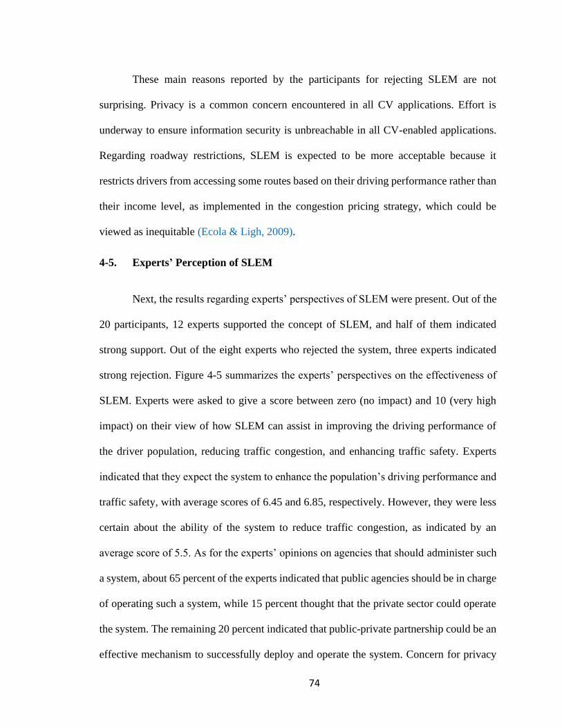
74
These main reasons reported by the participants for rejecting SLEM are not
surprising. Privacy is a common concern encountered in all CV applications. Effort is
underway to ensure information security is unbreachable in all CV-enabled applications.
Regarding roadway restrictions, SLEM is expected to be more acceptable because it
restricts drivers from accessing some routes based on their driving performance rather than
their income level, as implemented in the congestion pricing strategy, which could be
viewed as inequitable (Ecola & Ligh, 2009).
4-5. Experts’ Perception of SLEM
Next, the results regarding experts’ perspectives of SLEM were present. Out of the
20 participants, 12 experts supported the concept of SLEM, and half of them indicated
strong support. Out of the eight experts who rejected the system, three experts indicated
strong rejection. Figure 4-5 summarizes the experts’ perspectives on the effectiveness of
SLEM. Experts were asked to give a score between zero (no impact) and 10 (very high
impact) on their view of how SLEM can assist in improving the driving performance of
the driver population, reducing traffic congestion, and enhancing traffic safety. Experts
indicated that they expect the system to enhance the population’s driving performance and
traffic safety, with average scores of 6.45 and 6.85, respectively. However, they were less
certain about the ability of the system to reduce traffic congestion, as indicated by an
average score of 5.5. As for the experts’ opinions on agencies that should administer such
a system, about 65 percent of the experts indicated that public agencies should be in charge
of operating such a system, while 15 percent thought that the private sector could operate
the system. The remaining 20 percent indicated that public-private partnership could be an
effective mechanism to successfully deploy and operate the system. Concern for privacy
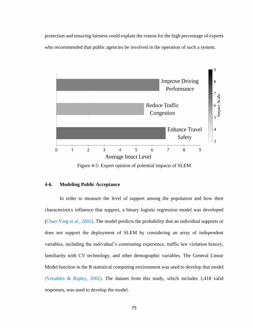
75
protection and ensuring fairness could explain the reason for the high percentage of experts
who recommended that public agencies be involved in the operation of such a system.
Figure 4-5: Expert opinion of potential impacts of SLEM
4-6. Modeling Public Acceptance
In order to measure the level of support among the population and how their
characteristics influence that support, a binary logistic regression model was developed
(Chao-Ying et al., 2002). The model predicts the probability that an individual supports or
does not support the deployment of SLEM by considering an array of independent
variables, including the individual’s commuting experience, traffic law violation history,
familiarity with CV technology, and other demographic variables. The General Linear
Model function in the R statistical computing environment was used to develop that model
(Venables & Ripley, 2002). The dataset from this study, which includes 1,418 valid
responses, was used to develop the model.

76
Table 4-4: Comparison among different model specifications
Coefficient Full Model Model 1
(Univariate)
Model 2
(Selection)
Model 3
(Stepwise)
Model 4
(Reduced)
Number of Variables 34 29 20 17 11
Number of Parameters 116 85 78 52 28
McFadden's R2 0.18 0.16 0.15 0.15 0.11
Nagelkerke R2 0.29 0.26 0.25 0.24 0.19
Hosmer-Lemeshow 0.81 0.44 0.20 0.76 0.32
Log-Likelihood -741.48 -761.04 -769.32 -770.27 -806.37
AIC 1715 1692.08 1694.64 1644.55 1668.75
BIC 1895.39 1824.29 1815.96 1725.43 1712.30
Corrected AIC (CAIC) 1735.83 1703.06 1703.85 1648.59 1669.92
Model Prediction Accuracy 0.73 0.71 0.72 0.72 0.70
Several models were developed that differ in terms of their set of independent
variables (See Appendices B - E). Table 4-4 gives several goodness-of-fit measures for
these models. The table also gives the prediction accuracy for each model. A review of
these goodness-of-fit measures can be found in Harrell (2015). As shown in Table 4-4, the
full model considers all available variables. Model 1, the univariate model, was built by
conducting a univariate analysis for each variable and choosing variables with a p-value ≤
0.25 (Bursac et al., 2008). Model 2, the selection model, was built based on the best
predictors used for the random forest (ensemble learning method) performed for the
dataset. After all variables in the random forest model were included, the top 20 predictors
were picked and used to form the selection logit model. Model 3, the stepwise model, was
built using backward elimination, which performs a stepwise model selection by the least
Akaike Information Criterion (AIC) value (Venables & Ripley, 2002). As shown in Table
4-4, the stepwise model gives the best AIC, Bayesian information criterion (BIC), and R2
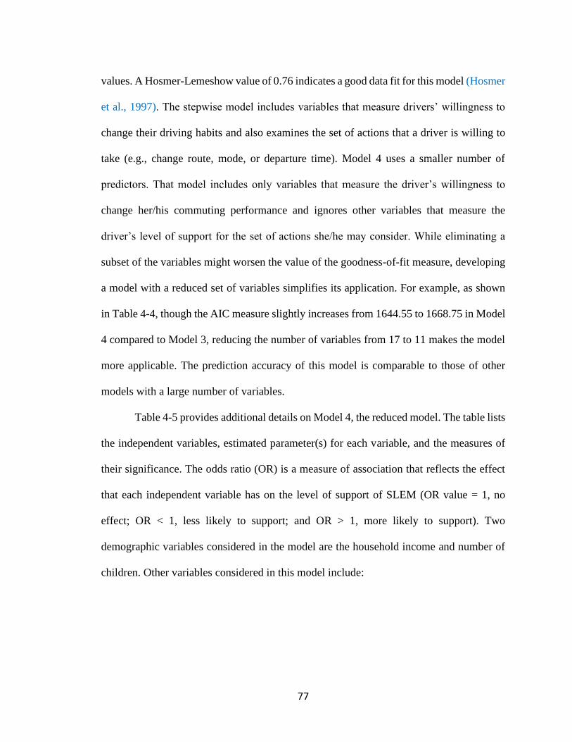
77
values. A Hosmer-Lemeshow value of 0.76 indicates a good data fit for this model (Hosmer
et al., 1997). The stepwise model includes variables that measure drivers’ willingness to
change their driving habits and also examines the set of actions that a driver is willing to
take (e.g., change route, mode, or departure time). Model 4 uses a smaller number of
predictors. That model includes only variables that measure the driver’s willingness to
change her/his commuting performance and ignores other variables that measure the
driver’s level of support for the set of actions she/he may consider. While eliminating a
subset of the variables might worsen the value of the goodness-of-fit measure, developing
a model with a reduced set of variables simplifies its application. For example, as shown
in Table 4-4, though the AIC measure slightly increases from 1644.55 to 1668.75 in Model
4 compared to Model 3, reducing the number of variables from 17 to 11 makes the model
more applicable. The prediction accuracy of this model is comparable to those of other
models with a large number of variables.
Table 4-5 provides additional details on Model 4, the reduced model. The table lists
the independent variables, estimated parameter(s) for each variable, and the measures of
their significance. The odds ratio (OR) is a measure of association that reflects the effect
that each independent variable has on the level of support of SLEM (OR value = 1, no
effect; OR < 1, less likely to support; and OR > 1, more likely to support). Two
demographic variables considered in the model are the household income and number of
children. Other variables considered in this model include:
78
• Driver’s opinion on the level of congestion encountered during her/his commute.
• Number of tickets issued in the past 5 years.
• Presence of any points on driver’s license.
• Driver’s willingness to change commuting behavior to reduce congestion.
• Driver’s anticipation of her/his score if the new system were deployed (this variable
gives information on the driver self-assessment of her/his driving performance).
• Driver’s familiarity with the CV and telematics technology.
• Driver’s acceptance of driving license suspension as a punishment for driving violation
(this variable was used to imply the driver’s level of acceptance to roadway access
restriction).

79
Table 4-5: The logistic regression model results (Reduced Model)
Coefficient Estimate Odds
Ratio 95% CI
Z-
Value
P-
Value
Driving Experience
(Reference = Less Than 4 Years)
4-10 Years -0.68 0.51 (-1.19, -0.2) -2.70 0.01 11-20 Years -0.83 0.44 (-1.35, -0.33) -3.20 0.00 More Than 20 Years -0.68 0.5 (-1.21, -0.18) -2.6 0.01
Weekly Commuting [Days] 0.05 1.05 (-0.01, 0.11) 1.54 0.12 Number of Tickets [Last 5 Years] 0.21 1.23 (0.03, 0.39) 2.30 0.02 Points on DL (Reference = No)
Yes 0.39 1.48 (-0.04, 0.84) 1.76 0.08
Congestion is a Commute Problem
(Reference = Strongly Disagree)
Somewhat Disagree 0.31 1.36 (-0.22, 0.84) 1.14 0.25 Neutral 0.77 2.17 (0.21, 1.34) 2.69 0.01 Somewhat Agree 0.65 1.92 (0.21, 1.09) 2.88 0.00 Strongly Agree 0.34 1.41 (-0.11, 0.79) 1.51 0.13
Willingness to Change Commuting
Routine (Reference = Extremely
Unlikely)
Somewhat Unlikely 0.40 1.49 (-0.67, 1.5) 0.73 0.47 Neutral 0.43 1.54 (-0.54, 1.45) 0.86 0.39 Somewhat Likely 1.02 2.77 (0.04, 2.03) 2.03 0.04 Extremely Likely 1.3 3.68 (0.32, 2.32) 2.58 0.01
DL Suspension as Punishment
(Reference = Strongly Disagree)
Somewhat Disagree 0.80 2.22 (-0.54, 2.17) 1.17 0.24 Neutral 1.09 2.99 (-0.1, 2.33) 1.78 0.07 Somewhat Agree 1.2 3.32 (0.1, 2.35) 2.12 0.03 Strongly Agree 1.52 4.55 (0.42, 2.66) 2.69 0.01
CVs Familiarity
(Reference = No)
Yes 0.34 1.40 (0.05, 0.62) 2.31 0.02 Expected Score (Reference = Excellent)
Poor -3.05 0.05 (-6.15, -0.77) -2.46 0.01
Fair -1.67 0.19 (-2.42, -0.93) -4.41 0.00
Good -1.16 0.31 (-1.53, -0.8) -6.26 0.00
Very Good -0.72 0.49 (-1.02, -0.42) -4.7 0.00
Number of Children 0.17 1.19 (0.05, 0.3) 2.83 0.00
Household Income
(Reference = < $50,000)
$50,000-$99,999 0.24
1.27 (-0.04, 0.51) 1.66 0.10 $100,000-$150,000 0.58 1.79 (0.18, 0.99) 2.83 0.00 > $150,000 0.68
1.98 (0.25, 1.13) 3.03 0.00
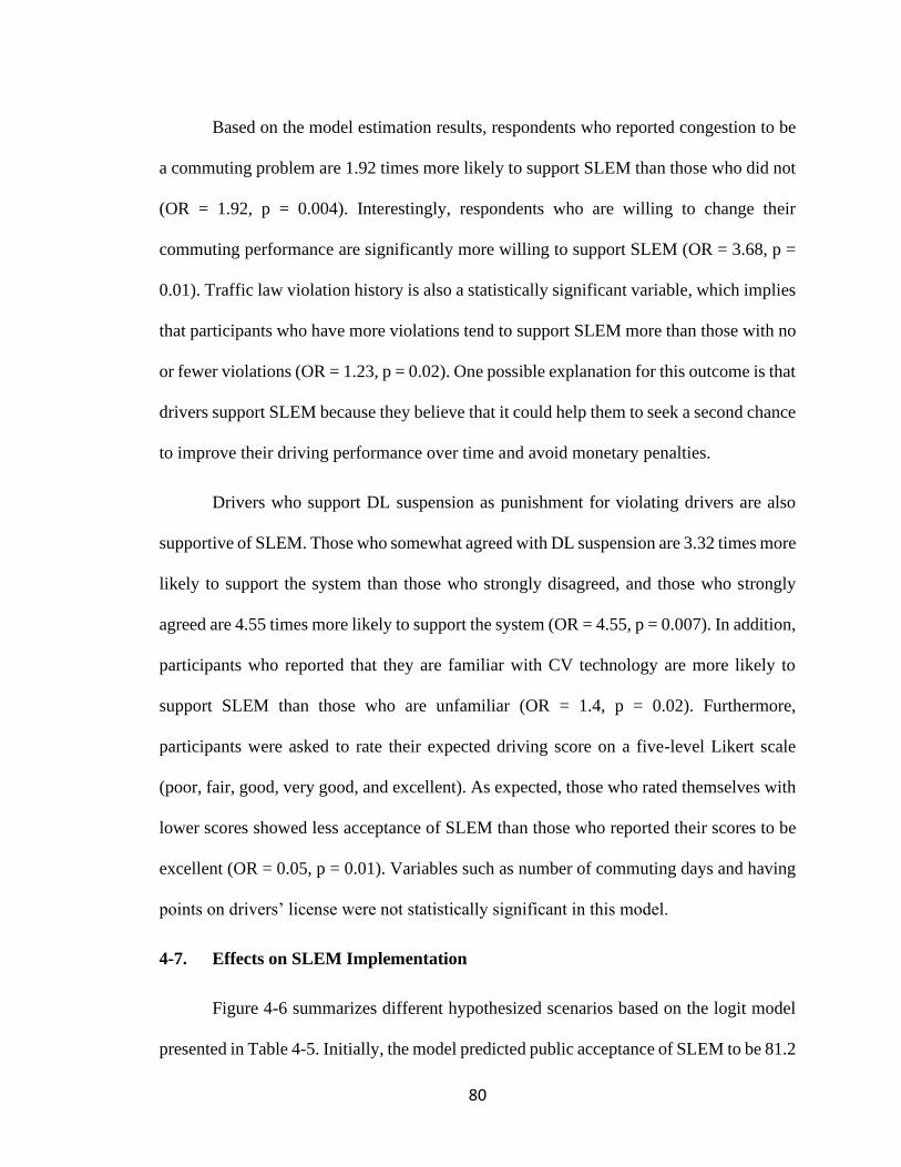
80
Based on the model estimation results, respondents who reported congestion to be
a commuting problem are 1.92 times more likely to support SLEM than those who did not
(OR = 1.92, p = 0.004). Interestingly, respondents who are willing to change their
commuting performance are significantly more willing to support SLEM (OR = 3.68, p =
0.01). Traffic law violation history is also a statistically significant variable, which implies
that participants who have more violations tend to support SLEM more than those with no
or fewer violations (OR = 1.23, p = 0.02). One possible explanation for this outcome is that
drivers support SLEM because they believe that it could help them to seek a second chance
to improve their driving performance over time and avoid monetary penalties.
Drivers who support DL suspension as punishment for violating drivers are also
supportive of SLEM. Those who somewhat agreed with DL suspension are 3.32 times more
likely to support the system than those who strongly disagreed, and those who strongly
agreed are 4.55 times more likely to support the system (OR = 4.55, p = 0.007). In addition,
participants who reported that they are familiar with CV technology are more likely to
support SLEM than those who are unfamiliar (OR = 1.4, p = 0.02). Furthermore,
participants were asked to rate their expected driving score on a five-level Likert scale
(poor, fair, good, very good, and excellent). As expected, those who rated themselves with
lower scores showed less acceptance of SLEM than those who reported their scores to be
excellent (OR = 0.05, p = 0.01). Variables such as number of commuting days and having
points on drivers’ license were not statistically significant in this model.
4-7. Effects on SLEM Implementation
Figure 4-6 summarizes different hypothesized scenarios based on the logit model
presented in Table 4-5. Initially, the model predicted public acceptance of SLEM to be 81.2
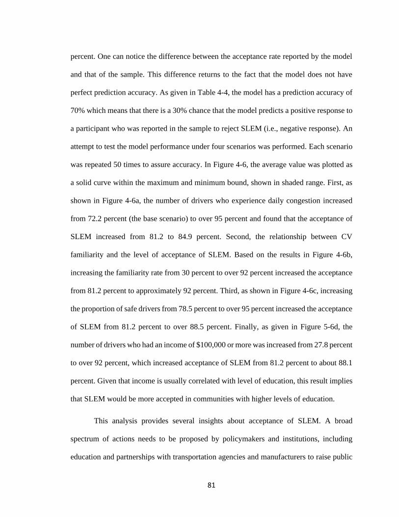
81
percent. One can notice the difference between the acceptance rate reported by the model
and that of the sample. This difference returns to the fact that the model does not have
perfect prediction accuracy. As given in Table 4-4, the model has a prediction accuracy of
70% which means that there is a 30% chance that the model predicts a positive response to
a participant who was reported in the sample to reject SLEM (i.e., negative response). An
attempt to test the model performance under four scenarios was performed. Each scenario
was repeated 50 times to assure accuracy. In Figure 4-6, the average value was plotted as
a solid curve within the maximum and minimum bound, shown in shaded range. First, as
shown in Figure 4-6a, the number of drivers who experience daily congestion increased
from 72.2 percent (the base scenario) to over 95 percent and found that the acceptance of
SLEM increased from 81.2 to 84.9 percent. Second, the relationship between CV
familiarity and the level of acceptance of SLEM. Based on the results in Figure 4-6b,
increasing the familiarity rate from 30 percent to over 92 percent increased the acceptance
from 81.2 percent to approximately 92 percent. Third, as shown in Figure 4-6c, increasing
the proportion of safe drivers from 78.5 percent to over 95 percent increased the acceptance
of SLEM from 81.2 percent to over 88.5 percent. Finally, as given in Figure 5-6d, the
number of drivers who had an income of $100,000 or more was increased from 27.8 percent
to over 92 percent, which increased acceptance of SLEM from 81.2 percent to about 88.1
percent. Given that income is usually correlated with level of education, this result implies
that SLEM would be more accepted in communities with higher levels of education.
This analysis provides several insights about acceptance of SLEM. A broad
spectrum of actions needs to be proposed by policymakers and institutions, including
education and partnerships with transportation agencies and manufacturers to raise public

82
awareness of the safety advantages of SLEM. Educating people about CV technology is a
key element of achieving this goal, since this study revealed that more than 70 percent (N
= 1000) of the participants were not aware of CV technology. Although acceptance of
SLEM was 65.7 percent, it is necessary to mention that 15.5 percent (N = 221) reported
that privacy concerns were their only reason for rejecting this policy, which emphasizes
the fact that raising awareness and educating the public could boost the acceptance of this
policy to over 80 percent. In addition, about 2.19 percent (N = 31) of participants reported
that they rejected the SLEM because they believed it could not be deployed. Addressing
concerns over privacy and demonstrating an operational system could increase the public
acceptance to over 83 percent.
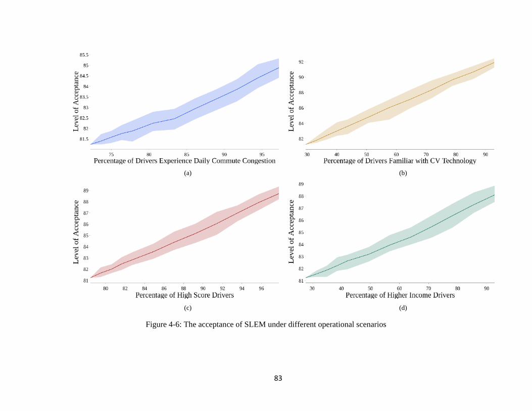
83
(a) (b)
(c) (d)
Figure 4-6: The acceptance of SLEM under different operational scenarios
84
4-8. Summary and Discussion
Several issues related to the deployment of SLEM are worth discussion. First, the
SLEM is an autonomous system with built-in traffic violation detection capabilities. These
capabilities could be expanded through installation of appropriate sensors to detect other
severe violations, such as driving under influence and hit-and-run incidents. Expanding
these capabilities would significantly reduce dependence on traditional policing operations
for enforcing the law against these felonies. Second, intensive research will be required to
determine the weight of each detected traffic violation in the overall score assigned to each
driver. These weights could vary by community or based on the prevailing traffic
conditions in the network. For example, a single-occupancy vehicle in an HOV lane might
be assigned a higher penalty in the peak periods as compared to a penalty assigned outside
the peak periods. Third, the overall purpose of SLEM is to improve compliance with
driving laws in a more equitable way. Therefore, differentiating between innocent and
intentional violations is important for achieving public trust of SLEM. Fourth, the score
could be extended to incorporate other factors in addition to driving performance. The
score could include measures such as the vehicle’s level of maintenance as an incentive for
drivers to routinely maintain the minimum legal safety requirement of their vehicles. In
addition, incentives could be offered for drivers to improve their scores. For example,
drivers who reduce the total number of miles traveled, reduce their traveled miles in the
peak period, or increase their dependence on transit and non-motorized vehicles could be
eligible for score improvements.

85
Chapter 5
THE SCORE-BASED TRAFFIC LAW-ENFORCEMENT AND NETWORK
MANAGEMENT SYSTEM: PROBLEM DEFINITION AND FORMULATION
5-1. Introduction
This chapter describes the proposed score-based traffic law-enforcement and
network management system (SLEM). First, the main assumptions considered for SLEM
are listed. Then, the theories of user equilibrium and system optimal for traffic network are
described. A formal definition of the problem is then given, followed by its mathematical
formulation. This chapter is organized as follows. Section 5-2 gives the assumptions that
were considered for designing SLEM. A background of SO and UE traffic assignments is
then provided in section 5-3. The problem definition followed by the mathematical
formulation are then introduced in sections 5-4 and 5-5, respectively. Finally, a summary
of chapter 5 is then provided in section 5-6.
5-2. Main Assumptions
This chapter introduces the mathematical model for SLEM. Several assumptions
are considered for the system:
(a) A vehicle-to-infrastructure (V2I) secured connected system is established across the
entire roadway network, which is capable of collecting high-frequency real-time data
describing the location, movement direction, speed, acceleration, steering wheel angle,
and tailgating distance for each vehicle on the road. The system can also obtain real-

86
time information on the status of each traffic light. The system is connected to a database
describing the speed limit for all links and all mandatory signs in the network.
(b) SLEM is equipped with built-in rules that can be applied to reliably detect traffic
law violations such as running a red light, violating the speed limit, tailgating, and
performing a prohibited maneuver, etc.
(c) Each vehicle trip has an identified registered driver linked to it. Drivers have
knowledge of SLEM and its functionality as an integrated law enforcement and traffic
network management system.
(d) SLEM assigns each driver a score that reflects her/his average performance over a pre-
defined period. This score is used to determine the driver’s eligibility for route access
for her/his current trip.
(e) Each driver can get a record of her/his violations in real-time along with instructions
and incentives to improve her/his current score. Drivers who consistently fail to adhere
to the traffic laws are subject to severe penalties ranging from imposing points on driver
license to driving license suspension or jail time.
5-3. User Equilibrium and System Optimal: A Brief Review
We defined 𝑆 as the list of possible score levels that a driver could be assigned such
that 𝑠1 > 𝑠2 implies that drivers with score 𝑠1 have a higher driving performance than those
with score level 𝑠2. Two dynamic traffic route assignment strategies are considered: (a)
dynamic user equilibrium (DUE) and (b) dynamic system optimal (DSO) (Peeta &
Mahmassani, 1995). Each pattern defines a set of superior routes for each origin-
destination (OD) pair and departure time interval that are used by the drivers. The DUE
pattern assumes that each driver selects the route that minimizes her/his travel time under
87
a perfect information scenario. At equilibrium, no driver can improve her/his travel time
by unilaterally changing her/his route. In the DSO routing strategy, drivers are assumed to
fully comply with a route guidance strategy in which they are assigned to routes that
minimize the total network travel time. Under the DSO equilibrium, no driver can improve
her/his marginal travel time by unilaterally changing her/his route.
A successful traffic management strategy would shift the traffic route assignment
pattern in the network from the undesirable DUE pattern to the desirable DSO pattern in
order to minimize the total travel time in the network. SLEM determines a route restriction
scheme, which is defined in terms of the lowest (worst) score threshold for each route such
that drivers with scores equal to or higher than this threshold are allowed to use this route.
Assuming that drivers are choosing routes that minimize their travel time in the network,
these thresholds are determined such that the traffic pattern in the network is transformed
from DUE toward the DSO pattern. In other words, the threshold value for each route is
strategically determined such that (a) the total travel time in the network is minimized, and
(b) drivers with high scores are assigned high travel priority and may access faster routes
in the network.
5-4. Problem Definition
Notations:
𝐺(. ) : A directed network
𝑁 : The set of nodes in 𝐺 indexed by 𝑖 and 𝑗
𝐴 : The set of roadway links in 𝐺 indexed by 𝑎
𝑇 : The horizon of interest which includes |𝑇| departure time intervals and |𝑇′| link
observation intervals

88
𝑡 : Observation interval, 𝑡 = 1,…, |𝑇|
𝑆 : The set of driving performance score classes indexed by 𝑠 (𝑠𝑛 is performing better
than 𝑠𝑛+1)
𝐾 : The set of superior routes in 𝐺 indexed by 𝑘
𝜏 : Departure time interval, 𝜏 = 1,…, |𝑇′|
𝑑𝑖𝑗𝜏 : Number of vehicles traveling from origin 𝑖 to destination 𝑗 at departure interval 𝜏
𝑑𝑖𝑗𝑠𝜏 : Number of vehicles traveling from origin 𝑖 to destination 𝑗 at departure interval 𝜏
by drivers belonging to score class 𝑠
𝜂𝑖𝑗𝑠𝜏 : Percentage of vehicles traveling from origin 𝑖 to destination 𝑗 at departure interval
𝜏 with by drivers belonging to score class 𝑠.
𝑑𝑖𝑗𝑘𝜏 : Number of vehicles traveling from origin 𝑖 to destination 𝑗 at departure interval 𝜏
using route 𝑘
𝑑𝑖𝑗𝑘𝑠𝜏 : Number of vehicles traveling from origin 𝑖 to destination 𝑗 at departure interval 𝜏
using route 𝑘 by drivers belonging to score class 𝑠
𝑐𝑖𝑗𝑘𝜏 : Minimum driving performance score allowed to travel from origin 𝑖 to destination
𝑗 using route 𝑘 at departure interval 𝜏
𝑡𝑡𝑖𝑗𝑘𝜏 : The travel time of route 𝑘 between origin-destination pair 𝑖 − 𝑗 at departure
interval 𝜏
𝜇𝑖𝑗𝑘𝑠𝜏 : A binary decision variable that is equal to one if a driver of class 𝑠 can use route
𝑘 between OD pair 𝑖 − 𝑗 in departure interval 𝜏, and zero otherwise.
𝑥𝑎𝑡 : The traffic flow on link 𝑎 at time interval 𝑡
𝑥𝑎𝑠𝑡 : The traffic flow from class 𝑠 on link 𝑎 at interval 𝑡
𝛿𝑖𝑗𝑘𝜏−𝑎𝑡 : An element in the route-link incidence matrix, which is equal to one if link 𝑎 in
interval 𝑡 ∈ |𝑇′| is part of route 𝑘 connecting OD pair 𝑖 − 𝑗 in departure interval
𝜏 ∈ 𝑇, and zero otherwise.
𝑡𝑡𝑎𝑡 (𝑥𝑎
𝑡 ) : The travel time of link 𝑎 in observation interval 𝑡
Consider a roadway network 𝐺(𝑁, 𝐴, 𝐷), where 𝑁 is the set of nodes, 𝐴 is the set
of links, and 𝐷 is the time-dependent traffic demand pattern defined for the network for a
pre-defined horizon of interest 𝑇. This horizon includes |𝑇| departure time intervals and

89
|𝑇′| link observation intervals. The vehicle demand 𝑑𝑖𝑗𝜏 ∈ 𝐷 for each origin-destination
(OD) pair 𝑖 − 𝑗 ∈ 𝑁 and departure interval 𝜏 ∈ 𝑇 is assumed given. Assume the existence
of a CV environment that enables the development of a telematics platform to infer reliable
information on the driving performance of each driver. With this platform, drivers could
be assigned scores that reflect their driving performance over a pre-defined past horizon or
for a certain number of past trips. A high number of violations indicates a low driving
performance score, and vice versa. We define 𝑆 as the list of possible score classes that
could be assigned to drivers such that 𝑠1 > 𝑠2 implies that drivers assigned to level 𝑠1
exhibit a better (i.e., higher) driving performance than those assigned to level 𝑠2. For each
OD pair 𝑖 − 𝑗 and departure interval 𝜏, the driver score distribution is assumed to be given,
where 𝜂𝑖𝑗𝑠𝜏 is the percentage of drivers belonging to class 𝑠 ∈ 𝑆. Here, the number of score
classes |𝑆| for any OD pair and departure time interval is defined such that the number of
vehicles in each class is much smaller than the capacity of any of the roadway links in the
network. Thus, no link will be saturated by the vehicles of one score class of a given OD
pair and departure time interval, which provides flexibility for SLEM to assign the traffic
obtaining a pattern that is close to that of the SO one. We define 𝑑𝑖𝑗𝑠𝜏 as the number of
drivers traveling between OD pair 𝑖 − 𝑗 in departure interval 𝜏 and belonging to score class
𝑠 ∈ 𝑆.
Each route 𝑘 that connects an OD pair 𝑖 − 𝑗 at departure interval 𝜏 is allocated a
minimum score threshold 𝑐𝑖𝑗𝑘𝜏. Drivers belonging to a score class 𝑠 ∈ 𝑆 that is less than
𝑐𝑖𝑗𝑘𝜏 are restricted from using that route or any other route with a score threshold greater
than 𝑠. Drivers who do not comply with such route access restrictions mandated by the

90
system expect to see their scores worsen and could be subjected to other penalties. Figure
5-1 displays an OD pair having three routes connecting them. Drivers employing one of
these routes and traveling from origin to destination are assigned to one of three
performance score levels ranked from highest (s=1) to lowest (s=3). In this example, the
score threshold for Route 1 equals 2, implying that only drivers belonging to score classes
1 and 2 (𝑑𝑖𝑗1𝜏 and 𝑑𝑖𝑗2
𝜏 ) are eligible to use this route. Similarly, Route 2’s score level is equal
to 1, thus limiting access to this route to drivers belonging to the highest driving
performance class (𝑑𝑖𝑗1𝜏 ).
Figure 5-1: Access eligibility for three routes with different score thresholds
Vehicles traveling between an OD pair in any given departure time interval are
assigned to a superior set of routes 𝐾 connecting this OD pair. We assume that the routes
belonging to this set are sorted in descending order based on their travel time values. Thus,
a route with a low index has less travel time than that of a route with a high index. We
define 𝑑𝑖𝑗𝑘𝜏 as the number of vehicles that travel between OD pair 𝑖 − 𝑗 in departure interval
Eligible Demand of
Route 1: 𝑑𝑖𝑗 1𝜏 & 𝑑𝑖𝑗 2
𝜏
Eligible Demand of
Route 2: 𝑑𝑖𝑗 1𝜏
𝑆 = 1,2,3
𝑑𝑖𝑗𝑠𝜏
Eligible Demand of Route 3:
𝑑𝑖𝑗 1𝜏 , 𝑑𝑖𝑗 2
𝜏 & 𝑑𝑖𝑗 3𝜏

91
𝜏 ∈ 𝑇 using route 𝑘 ∈ 𝐾. The level of congestion on each route is measured in terms of the
route travel time 𝑡𝑡𝑖𝑗𝑘𝜏 (. ). The portion of vehicles with drivers who belong to score class
𝑠 ∈ 𝑆 and use route 𝑘 ∈ 𝐾 is defined as 𝑑𝑖𝑗𝑘𝑠𝜏 . The binary decision variable 𝜇𝑖𝑗𝑘𝑠
𝜏 indicates
whether a vehicle with a driver of class 𝑠 ∈ 𝑆 is eligible to use route 𝑘 ∈ 𝐾 connecting OD
pair 𝑖 − 𝑗 in departure interval 𝜏 ∈ 𝑇. The corresponding traffic flow 𝑥𝑎𝑠𝑡 from class 𝑠 ∈ 𝑆
on link 𝑎 ∈ 𝐴 in observation interval 𝑡 ∈ 𝑇′ can hence be defined using the information of
the assignment matrix 𝛿𝑖𝑗𝑘𝜏−𝑎𝑡 ∀ 𝑖, 𝑗, 𝑘, 𝑎, 𝜏, 𝑡, which maps the route flows to the link flows.
Finally, we define 𝑥𝑎𝑡 and 𝑡𝑡𝑎
𝑡 (𝑥𝑎𝑡 ) as the total flow and corresponding travel time of link
𝑎 ∈ 𝐴 in interval 𝑡 ∈ 𝑇′, respectively.
5-5. Mathematical Formulation
The route score thresholds 𝑐𝑖𝑗𝑘𝜏 ∀ 𝑖, 𝑗, 𝑘, 𝜏 constitute the problem’s decision
variables, and these are determined so as to minimize total travel time in the network while
assuming that travelers are exhibiting a route choice behavior that they perceive as
minimizing their travel times. The formulation ensures that drivers having high scores can
access faster routes in the network, while restricting those having low scores to slower
routes within the network. The mathematical formulation for this problem is as follows:

92
Minimize ∑ ∑ ∑ (∑ 𝑑𝑖𝑗𝑘𝑠𝜏
𝑠≥𝑐𝑖𝑗𝑘𝜏) . 𝑡𝑡𝑖𝑗𝑘
𝜏𝜏𝑘𝑖𝑗 (1)
Subject to:
𝑑𝑖𝑗𝑘𝑠𝜏 = 0 ∀ 𝑖, 𝑗, 𝑘, 𝜏, 𝑠 < 𝑐𝑖𝑗𝑘𝜏 (2)
𝑡𝑡𝑖𝑗𝑘𝜏 ∙ 𝜇𝑖𝑗𝑘𝑠
𝜏 ≤ 𝑡𝑡𝑖𝑗𝑘′𝜏 ∙ 𝜇𝑖𝑗𝑘′𝑠′
𝜏 ∀ 𝑖, 𝑗, 𝑘, 𝑘′, 𝜏, 𝑠 ≥ 𝑠′, 𝜇𝑖𝑗𝑘′𝑠′𝜏 > 0 (3)
𝑐𝑖𝑗𝑘𝜏 is a positive integer ∀ 𝑖, 𝑗, 𝜏, 𝑘 (4)
∑ 𝛿𝑖̅�̅��̅�𝜏−𝑎𝑡 ∙ 𝜇𝑖̅�̅��̅��̅�
𝜏�̅�≤𝑘 + ∑ 𝜇𝑖̅�̅��̅��̅�
𝜏 + (∑ 𝜇𝑖̅�̅��̅��̅�𝜏 )�̅�≤𝑘 ∙ (1 − 𝛿𝑖̅�̅�𝑘
𝜏−𝑎𝑡) ≥ 𝛿𝑖𝑗𝑘𝜏−𝑎𝑡 ∙�̅�≤𝑘 𝜇𝑖𝑗𝑘𝑠
𝜏
∀ 𝑎, 𝑖, 𝑗, 𝑖,̅ 𝑗,̅ 𝑘, �̅�, 𝜏, �̅� = 𝑠 − 1 (5)
Minimize ∑ ∑ ∫ 𝑡𝑡𝑎𝑡 (∑ 𝑣𝑎𝑠
𝑡𝑠 )𝑑𝑣
𝑥𝑎𝑡
0𝑡𝑎 (6)
Subject to:
𝑑𝑖𝑗𝜏 = ∑ ∑ ∑ 𝑑𝑖𝑗𝑘
𝜏𝑘𝜏𝑖𝑗 ∀ 𝑖, 𝑗, 𝜏 (7)
𝑑𝑖𝑗𝑘𝜏 = ∑ 𝑑𝑖𝑗𝑘𝑠
𝜏𝑠 ∀ 𝑖, 𝑗, 𝑘, 𝜏 (8)
𝑑𝑖𝑗𝑠𝜏 = ∑ 𝑑𝑖𝑗𝑘
𝜏𝑘 ∀ 𝑖, 𝑗, 𝑘, 𝜏 (9)
𝑥𝑎𝑡 = ∑ ∑ ∑ (∑ 𝛿𝑖𝑗𝑘
𝜏−𝑎𝑡. 𝑑𝑖𝑗𝑘𝑠𝜏
𝑠≥𝑐𝑖𝑗𝑘𝜏)𝜏𝑘𝑖𝑗 ∀ 𝑖, 𝑗, 𝑘, 𝜏 (10)
𝑥𝑎𝑠𝑡 = ∑ ∑ ∑ 𝛿𝑖𝑗𝑘
𝜏−𝑎𝑡. 𝑑𝑖𝑗𝑘𝑠𝜏
𝜏𝑘𝑖𝑗 ∀ 𝑖, 𝑗, 𝑘, 𝜏, 𝑠 ≥ 𝑐𝑖𝑗𝑘𝜏 (11)
𝑡𝑡𝑖𝑗𝑘𝜏 = ∑ 𝛿𝑖𝑗𝑘
𝜏−𝑎𝑡 ∙ 𝑡𝑡𝑎𝑡 (𝑥𝑎
𝑡 )𝑎 ∀ 𝑖, 𝑗, 𝑘, 𝜏 (12)
𝑑𝑖𝑗𝑘𝑠𝜏 ≥ 0 ∀ 𝑖, 𝑗, 𝜏, 𝑘, 𝑠 (13)

93
The problem is formulated in the form of a bi-level mathematical program. The
upper-level problem given in (1-5) determines the optimal score threshold for each route,
while the lower-level problem given in (6-13) captures the drivers' route choice behavior
in response to the thresholds determined in the upper-level problem. The objective function
given in (1) minimizes total travel time, i.e., the sum of the travel times of all vehicles in
the network. For each OD pair 𝑖 − 𝑗 and departure interval 𝜏, the demand of the different
score classes allowed on route 𝑘 is summed, and this total is then multiplied by the route’s
travel time.
The constraint in (2) restricts drivers from accessing routes with score thresholds
that are higher than their score levels. The constraint in (3) ensures that drivers with high
scores are accorded high travel priorities within the network. For instance, consider two
drivers traveling between node pair 𝑖 − 𝑗 at departure interval 𝜏 who belong to classes 𝑠
and 𝑠′ such that 𝑠 ≥ 𝑠′. If these two drivers are assigned to routes 𝑘 and 𝑘′, respectively,
route 𝑘’s travel time must be less than or equal to that of route 𝑘′. The constraint in (4)
specifies that the route score thresholds are positive integers. The constraint in (5) ensures
that drivers with higher scores are provided higher access priority at the link level,
irrespective of their OD pairs.
The lower-level problem solves for the user equilibrium dynamic traffic assignment
pattern that satisfies the route restriction constraints obtained from the upper-level problem.
The objective function in Equation (6) describes the dynamic user equilibrium (UE)
objective function. The flow conservation constraints at the OD, route, and score levels are
given in the constraints in (7)-(9), respectively. The constraints in (10) and (11) use the
assignment matrix to determine the link flows as a function of the route flows. Similarly,
94
the constraint in (12) calculates the travel time for each route. Finally, the non-negativity
of the route flows is guaranteed by the constraint in (13).
5-6. Summary
This chapter present a formal problem definition and the mathematic formulation
for SLEM. The problem is formulated as a bi-level mathematical program. The upper-level
problem minimizes the total travel time in the network under the optimal score threshold
for all the routes. The lower-level problem represents the travelers’ route choice behavior
assuming a user equilibrium traffic flow pattern. The next chapter present an efficient
solution methodology for this mathematic program.
95
Chapter 6
SOLUTION METHODOLOGY
6-1. Introduction
This section presents the solution algorithm developed for the problem described
in the previous chapter. A heuristic-based approach was adopted to obtain a sub-optimal
solution for the problem. This heuristic decomposes the problem into two sequential sub-
problems, the first of which solves the dynamic SO traffic flow pattern in the network. The
solution to this problem gives the time-varying path flows and their corresponding link
flows. The second sub-problem determines the optimal score threshold values for a given
driver population following its performance score distribution. These thresholds are
determined such that the resulting traffic flow pattern in the network is as close as possible
to the dynamic SO flow pattern obtained from solving the first sub-problem. This chapter
is organized as follows. Section 6-2 explains the steps of the solution algorithm and how
the heuristic algorithm obtains the score threshold allocated on each link on the traffic
network, as demonstrated in the accompanying. Finally, a summary of this chapter is
provided in section 6-3.
6-2. The Optimal Score Threshold
Finding the optimal solution for the bi-level mathematical program is a challenging
task. The program consists of upper-level and lower-level problems that are nonlinear

96
(Sheffi, 1985). In both problems, the flow pattern assigned to a path is a function of the
travel time of that path, which in return depends on the amount of traffic assigned to that
route. In addition, there is no guarantee of the convexity of the objective function given in
(1), given the discrete nature of the decision variables 𝑐𝑖𝑗𝑘𝜏 ∀ 𝑖, 𝑗, 𝑘 , 𝜏. To overcome these
difficulties, a heuristic-based approach was adopted to obtain a sub-optimal solution for
the problem. This heuristic decomposes the problem into two sequential sub-problems, the
first of which solves the dynamic SO traffic flow pattern in the network. The solution to
this problem gives the time-varying path flows and their corresponding link flows 𝑦𝑎𝑡 ∀ 𝑎, 𝑡.
The second sub-problem determines the optimal score threshold values 𝑐𝑖𝑗𝑘𝜏 ∀ 𝑖, 𝑗, 𝑘 , 𝜏 for
a given driver population with performance score distribution 𝑑𝑖𝑗𝑠𝜏 ∀ 𝑖, 𝑗, 𝑠 , 𝜏. These
thresholds are determined such that the resulting traffic flow pattern in the network is as
close as possible to the dynamic SO flow pattern obtained from solving the first sub-
problem.
The first sub-problem has been intensively studied in the literature. For example,
the pioneering work in (Peeta & Mahmassani, 1995) presents an iterative simulation-based
dynamic traffic assignment methodology to solve the dynamic SO traffic assignment
problem. Additional details on mathematical formulations and solution methodologies
developed for the dynamic SO problem can be found in (Merchant & Nemhauser, 1978;
Ziliaskopoulos, 2000). The second sub-problem can be described using the mathematical
program given in Equations (14) through (24). The objective function in (14) minimizes
the squared difference between the time-varying link flows under SLEM’s route guidance
strategy, 𝑥𝑎𝑡 ∀ 𝑎, 𝑡, and those associated with the dynamic SO traffic flow pattern, 𝑦𝑎
𝑡 ∀ 𝑎, 𝑡.
Similar to the formulation above, the constraint given in (15) determines the link flows

97
from the path flows, and the constraints in (16) and (17) ensure flow conservation at the
path and OD pair levels, respectively. The constraint in (18) determines if the demand of
OD pair 𝑖 − 𝑗 and departure time interval 𝜏 that belongs to class 𝑠 is eligible to use route 𝑘
or not. Class 𝑠 is eligible to use route 𝑘 only if the variable 𝜇𝑖𝑗𝑘𝑠𝜏 is equal to one. Given that
the routes between each OD are sorted in an ascending order based on their travel time
values, the constraint in (19) ensures that the shortest route is always available for drivers
with the highest performance (i.e., 𝑠 = 1). The constraint in (20) ensures that no better
route can be assigned to drivers with lower performance classes. The constraint in (21) is
the same as constraint (5) as described above. The constraint in (22) ensures that each class
of driver is assigned to one route. The non-negativity of the path flows is satisfied in the
constraint in (23). Finally, the constraint in (24) defines the variable 𝜇𝑖𝑗𝑘𝑠𝜏 as a binary
variable.
Minimize ∑ ∑ (𝑦𝑎𝑡 − 𝑥𝑎
𝑡 )2𝑡𝑎 (14)
Subject to:
𝑥𝑎𝑡 = ∑ ∑ ∑ (𝛿𝑖𝑗𝑘
𝜏−𝑎𝑡. 𝑑𝑖𝑗𝑘𝜏 )𝜏𝑘𝑖𝑗 ∀ 𝑖, 𝑗, 𝑘, 𝜏 (15)
𝑑𝑖𝑗𝑘𝜏 = ∑ 𝑑𝑖𝑗𝑘𝑠
𝜏𝑠 ∀ 𝑖, 𝑗, 𝑘, 𝜏 (16)
𝑑𝑖𝑗𝜏 = ∑ 𝑑𝑖𝑗𝑘
𝜏𝑘 ∀ 𝑖, 𝑗, 𝑘, 𝜏 (17)
𝑑𝑖𝑗𝑘𝑠𝜏 = 𝜇𝑖𝑗𝑘𝑠
𝜏 ∙ 𝜂𝑖𝑗𝑠𝜏 ∙ 𝑑𝑖𝑗
𝜏 ∀ 𝑖, 𝑗, 𝑘, 𝜏, 𝑠 (18)
𝜇𝑖𝑗𝑘𝑠𝜏 = 1 ∀ 𝑖, 𝑗, 𝑘 = 1, 𝑠 = 1 (19)
𝜇𝑖𝑗𝑘𝑠𝜏 ≤ ∑ 𝜇𝑖𝑗�̅�𝑠
𝜏�̅�≤𝑘 ∀ 𝑖, 𝑗, 𝑘, 𝜏, 𝑠, 𝑠 ∈ 𝑆 − (𝑠 = 1) (20)

98
∑ 𝛿𝑖̅�̅��̅�𝜏−𝑎𝑡 ∙ 𝜇𝑖̅�̅��̅��̅�
𝜏�̅�≤𝑘 + ∑ 𝜇𝑖̅�̅��̅��̅�
𝜏 + (∑ 𝜇𝑖̅�̅��̅��̅�𝜏 )�̅�≤𝑘 ∙ (1 − 𝛿𝑖̅�̅�𝑘
𝜏−𝑎𝑡) ≥ 𝛿𝑖𝑗𝑘𝜏−𝑎𝑡 ∙�̅�≤𝑘 𝜇𝑖𝑗𝑘𝑠
𝜏
∀ 𝑎, 𝑖, 𝑗, 𝑖,̅ 𝑗,̅ 𝑘, �̅�, 𝜏, �̅� = 𝑠 − 1 (21)
∑ 𝜇𝑖𝑗𝑘𝑠𝜏
𝑘 = 1 ∀ 𝑖, 𝑗, 𝑠 (22)
𝑑𝑖𝑗𝑘𝑠𝜏 ≥ 0 ∀ 𝑖, 𝑗, 𝜏, 𝑘, 𝑠 (23)
𝜇𝑖𝑗𝑘𝑠𝜏 ∈ (0,1) ∀ 𝑖, 𝑗, 𝜏, 𝑘, 𝑠 (24)
Figure 6-1 describes the main steps of the heuristic. As shown in the figure, the
methodology consists of two main steps that are solved sequentially. In the first step, the
dynamic SO problem is solved following the simulation-based assignment methodology
described in (Peeta & Mahmassani, 1995). At each iteration, the following steps are
implemented: (1) computing the time-varying link marginal travel time for all links in the
network; (2) determining the time-dependent least marginal travel time path for all OD
pairs and departure time intervals; (3) performing all-or-nothing traffic assignments using
the optimal paths obtained in step (2); (4) applying the method of successive averages to
update the time-varying path flows; and (5) checking for convergence by examining a pre-
defined stopping criteria. The solution to the dynamic SO traffic assignment problem gives
the time-varying path flows and their corresponding link flows 𝑦𝑎𝑡 ∀ 𝑎, 𝑡. The solution also
gives the list of paths connecting each OD pair at each departure time interval. These paths
are sorted in an ascending order based on their travel time values.
As mentioned earlier, the driver performance classes are set with high resolution
such that the number of drivers belonging to any one class is much less than the capacity
of roadway links. Thus, a link is not saturated by assigning the demand of one driver class

99
of any OD pair and departure time interval. Given this assumption, the second step
implements an all-or-nothing traffic assignment procedure to sequentially assign the
demand of each class for all departure time intervals. Driver classes are assigned to paths
such that the resulting flow pattern is as close as possible to the dynamic SO one. As shown
in the figure, for the first departure time interval (𝜏 = 1) in the time horizon and for a
randomly selected OD pair, 𝑖 − 𝑗, the heuristic assigns the driver class with the highest
performance (𝑠 = 1) to the SO path 𝑘 with the least travel time (i.e., the first path in the
SO paths list). The heuristic determines the residual flow, 𝑟𝑘𝜏𝑖𝑗
, for path 𝑘 by checking the
difference 𝑟𝑎𝑡 = 𝑦𝑎
𝑡 − 𝑥𝑎𝑡 ∀ 𝑎, 𝑡. If the difference 𝑟𝑎
𝑡 is less than or equal to zero for any of
the links of path 𝑘, this path is eliminated from the paths list of the departure time interval
𝜏 and the OD pair 𝑖 − 𝑗. The path 𝑘 is also marked as unavailable for all remaining classes.
The list of paths is then updated for all other OD pairs, 𝑖′ − 𝑗′ ≠ 𝑖 − 𝑗. Any path 𝑘′ between
OD pair 𝑖′ − 𝑗′ with 𝛿𝑖′𝑗′𝑘′𝜏−𝑎𝑡 = 1 and 𝑟𝑎
𝑡 ≤ 0 is removed from the paths list of OD pair 𝑖′ −
𝑗′ and departure time interval 𝜏. The process is repeated to assign the demand of the highest
performing driver class for all OD pairs in the current departure time interval. The process
then proceeds to assign the next driver class, continuing until the entire demand of the
current departure time interval is assigned. The steps are repeated for the next departure
time interval until the end of the time horizon is reached. The output includes the values of
𝜇𝑖𝑗𝑘𝑠𝜏 , ∀ 𝑖, 𝑗, 𝜏, 𝑘, 𝑠, which specifies the route available for each driver class (i.e., SLEM’s
route guidance strategy), and the resulting path assignment pattern 𝑑𝑖𝑗𝑘𝑠𝜏 , ∀ 𝑖, 𝑗, 𝜏, 𝑘, 𝑠. The
latter is used as input to a traffic network simulation model that estimates the overall
network performance under the generated route guidance strategy.
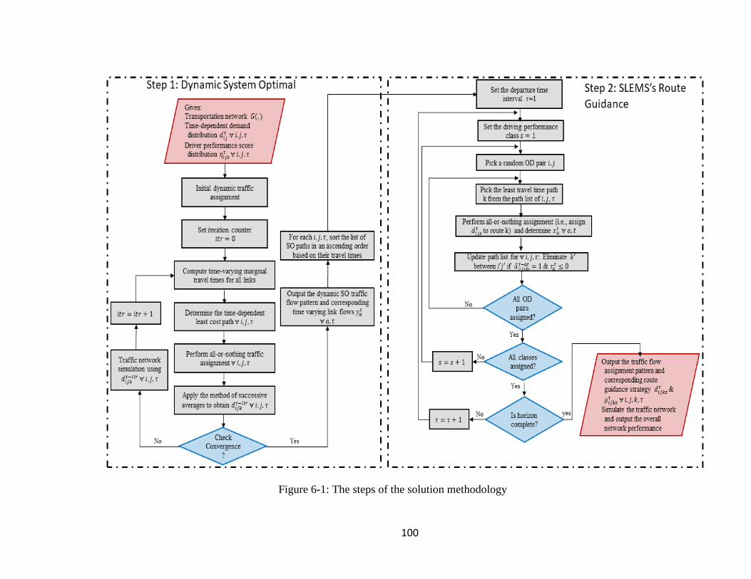
100
Figure 6-1: The steps of the solution methodology

101
6-3. Summary
In this chapter, we present the solution methodology for the score-based law
enforcement and traffic network management problem. Considering the problem
complexity, a heuristic-based approach was adopted. The heuristic‘s goal is to find a near-
optimal solution for the problem by decomposing the problem into two sequential sub-
problems. The first problem obtains the SO traffic flow pattern in the network which
provides the time-varying path flows and their corresponding link flows, where the second
sub-problem finds the optimal score threshold score for a given driver population. These
thresholds are then used to shift the traffic pattern from the undesirable UE to that is close
to the SO traffic pattern.
102
Chapter 7
EXPERIMENTS, RESULTS, AND ANALYSIS
7-1. Introduction
In this chapter, we present the results of a set of experiments that are designed to
evaluate SLEM performance under different operational scenario. These experiments
illustrate how SLEM could be used to shift the traffic pattern in the network for the
undesirable UE pattern to the SO pattern. In section 7-2, an overall description of the
experiment design and setup is provided. Section 7-3 provides a preliminary network
performance under the SO and UE traffic assignment to be compared as upper and lower
bound performance benchmarks. Sections 7-4 through 7-8 provide five different
experiments that were conducted to examine the effectiveness of SLEM’s route guidance
strategy under different operational scenarios to measure the effect of the scoring system
resolution, route assignment comparison, the effect of driver performance distribution,
SLEM’s performance under different compliance scenarios, and SLEM’s performance
under a non-recurrent incident, respectively. Finally, a summary of the results is provided
in section 7-9.
7-2. Testbed Network Description and Setup
A real road network with real demand was used as a testbed network. The network
includes about 25 miles of North Central Expressway (US-75) and parallel arterials. This

103
corridor is in Dallas, Texas. As shown in Figure 7-1, US-75 is a major commute corridor
which links the Dallas downtown in the south to northern Dallas cities such as Richardson,
Plano, and Allen. This corridor consists of a 4-lane per direction highway at most sections;
however, some sections have auxiliary-lanes. Furthermore, there is an HOV lane facility
added to its northern section which starts from the I-635 to the northern city of Allen, TX.
A light rail line is extended along the eastern side of US-75 which serves `the Dallas-Fort
Worth (DFW) metropolitan area. The US-75 corridor also includes an arterial network that
connects different cities within the DFW metropolitan area. The network includes 10,000
origin-destination (OD) pairs, 3,000 links, and 1,300 nodes with 365 signalized
intersections.
The used network is in the form of a corridor network which consists of two types
of traffic (i.e., serving two types of origin-destination pairs): a) longitudinal/main traffic
traveling along a main direction of the corridor (i.e., NS&SN directions); and b)
crossing/secondary traffic that cuts the corridor (short trips in EW&WE directions). Here,
the longitudinal traffic, which represents the movement of the commuters from the north
suburban areas to the downtown area, is the focus of our analysis. The crossing trips are
considered background traffic to make sure we capture the right congestion level on the
crossing arterials. We recorded the travel time savings for (1) all travelers in the network
(longitudinal and crossing) and (2) trips with travel distance greater than or equal to 10
miles, representing mainly the longitudinal trips. Based on the reported results, significant
savings were recorded for commuting traffic along the main direction of the corridor. Of
course, one can expect these benefits to be diluted as we consider all trips in the network
(main and secondary).

104
Figure 7-1: The testbed network used to evaluate SLEM’s route guidance strategy
7-3. Preliminary Network Performance Under UE and SO Travel Patterns
User Equilibrium and System Optimal traffic assignments were performed on the
US-75 network before conducting the set of experiments in order to check the convergence
rates and the final objective functions for both algorithms. Figure 7-2 shows the
convergence pattern of both UE and SO solution algorithms as the SO paths are used in the
next steps of the solution algorithm. Furthermore, the value of the objective function
resulting from SO and UE are compared against the objective function values generated by
the heuristic.
We envision the SLEM system as an operational planning tool that runs ahead of a
peak period to plan the route guidance strategy for that period. As discussed earlier, the
105
SLEM algorithm is executed in two main steps: the first step determines a System Optimal
traffic assignment pattern and the second step executes the SLEM route guidance
development. Using the Dell server machine (model PET636) equipped with 256 GB RAM
and two Xeon processors, each with 22 cores and 2.2 GHz, the first step is executed in less
than a minute while the second step is executed in 56 minutes for the 100 classes, which
would increase as the number of classes increases. Thus, the current computation time is
around one hour for the US-75 Corridor network used in this dissertation. This execution
time depends on two main elements: the network size (i.e., number of nodes, links, and
number of OD pairs) and number of performance score classes. Of course, adopting SLEM
as a real-time route guidance tool will require reducing its execution time. Strategies to
reduce the running time include (1) adopting penalization strategies (e.g., parallelizing the
assignment of the demand of OD pairs that are far from each other); and (2) the use of
warm starts that are obtained based on historical implementation of the system in previous
days with similar traffic patterns.
Several experiments are presented in this chapter which reflect different real-world
scenarios. The network configuration and the demand data are obtained based on a sub-
area analysis that is conducted to extract the US75 Corridor network from the Dallas-Fort
Worth regional model developed by North Central Texas Council of Government
(NCTCOG) (See: https://www.nctcog.org). This effort was conducted as part of a previous
project focusing on developing integrated corridor management strategies for the US75
Corridor (Hashemi & Abdelghany, 2016). Each experiment measures the performance of
SLEM in the traffic management given the assumed scenario. In order to measure its

106
performance, first the initial UE and SO performance are obtained as a benchmark result
which will be referred to in the experiments’ results.
As shown in Table 7-1, the morning peak hour between 7:00 – 8:00 AM was chosen
to be the base time of the experiment. It is the most congested time in the network with a
total demand of 279,809 travelers. For the UE travel assignment, the travelers used a total
of 14,816 paths to travel within the network with an average travel time of 11.63 minutes,
which resulted in a total travel time of 54,246.11 hours. The average travel distance and
speed were 6.45 miles and 33.26 miles/hour respectively. The SO travel assignment on the
other hand produced 23,912 paths in the network and, as expected, a lower average and
total travel time of 10.88 minutes and 50,742.65 hours. The SO average travel distance
increased to 6.59 miles and the average speed improved to 36.37 miles/hour. By comparing
the results of UE and SO assignments, as expected, the network was found to perform
better under the SO assignment with an overall 6.45 percent reduction in total network
travel time.
However, the nature of the testbed network (where arterials crossing from east to
west are generally shorter sections) resulted in relatively short average travel distances.
Therefore, besides reporting the total network performance, we considered reporting the
results of the remote ODs which are at least ten miles away. Table 7-1 shows the same
measures reported above for the remote ODs where UE generated 7,935 paths with average
distance of 14.47 miles and average travel time and an average speed of 25.09 minutes and
34.61 miles/hour respectively. The SO on the other hand produced a total of 13,963 paths
with slightly longer average distance of 14.55 miles and improved average travel time and

107
speed of 22.46 minutes and 38.87 miles/hour. These results clearly show a better network
performance when routes are longer, with an almost 9 percent improvement in travel time.

108
(a) SO algorithm (b) UE algorithm
Figure 7-2: Convergence curves for the SO and UE algorithms
45000
55000
65000
75000
85000
95000
0 50 100
Tra
vel
Tim
e
Iterations
45000
55000
65000
75000
85000
95000
0 20 40 60 80 100
Tra
vel
Tim
e
Iterations
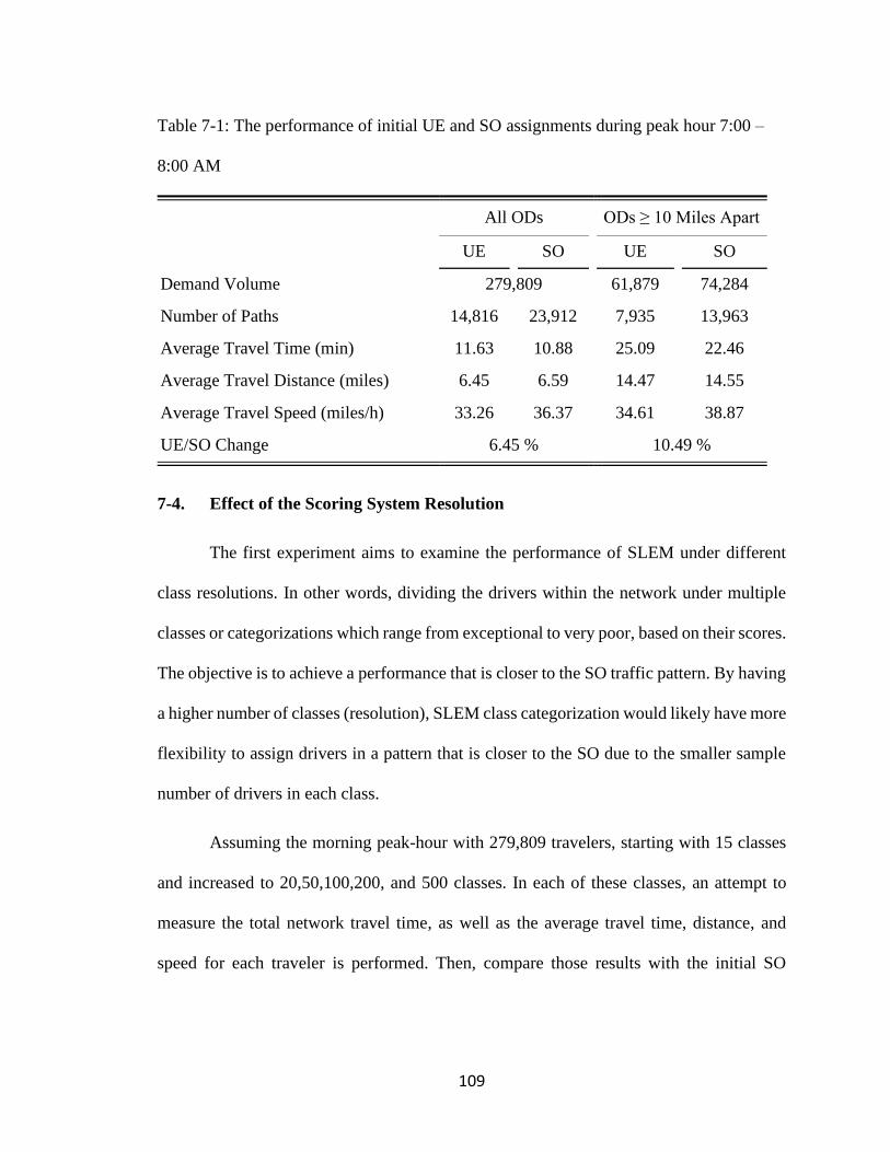
109
Table 7-1: The performance of initial UE and SO assignments during peak hour 7:00 –
8:00 AM
7-4. Effect of the Scoring System Resolution
The first experiment aims to examine the performance of SLEM under different
class resolutions. In other words, dividing the drivers within the network under multiple
classes or categorizations which range from exceptional to very poor, based on their scores.
The objective is to achieve a performance that is closer to the SO traffic pattern. By having
a higher number of classes (resolution), SLEM class categorization would likely have more
flexibility to assign drivers in a pattern that is closer to the SO due to the smaller sample
number of drivers in each class.
Assuming the morning peak-hour with 279,809 travelers, starting with 15 classes
and increased to 20,50,100,200, and 500 classes. In each of these classes, an attempt to
measure the total network travel time, as well as the average travel time, distance, and
speed for each traveler is performed. Then, compare those results with the initial SO
All ODs
ODs ≥ 10 Miles Apart
UE SO UE
SO
Demand Volume 279,809 61,879 74,284
Number of Paths 14,816
23,912 7,935 13,963
Average Travel Time (min) 11.63 10.88 25.09 22.46
Average Travel Distance (miles) 6.45 6.59 14.47 14.55
Average Travel Speed (miles/h) 33.26 36.37 34.61 38.87
UE/SO Change 6.45 % 10.49 %

110
benchmark performance reported in Table 7-1, such that the closest total travel time to the
initial SO travel time indicates a better result.
Table 7-2 summarized the overall performance of the SLEM traffic assignment
with respect to each class resolution case. An illustration of these results is also shown in
Figure 7-3. In the first case where travelers were distributed among 15 classes, the total
network travel time increased to 55,149.87 hours compared to the initial SO’s of 50,742.65
hours, with an almost 8.68 percent increase which resulted in a performance that is lower
than the UE. As a result, the average travel time, distance, and speed also increased to
11.826 minutes, 6.67 miles, 33.88 miles/hour respectively. By increasing the resolution to
20 classes, the total travel time improved to 53,260.49 hours, which is 4.95 percent away
from the SO traffic pattern. The average travel time and speed were also improved to
11.418 minutes and 35.11 miles/hour respectively. The average travel distance, on the other
hand, slightly increased to 6.67 miles per traveler. When a higher resolution experiment of
50 classes was conducted and compared to the 20 classes experiment, the SLEM produced
a better result in terms of total travel time of 52,066.05 hours which is closer to the SO
traffic pattern by 2.60 percent. Also, each of the average travel times, distance, and speed
were improved to 11.166 minutes, 6.67 miles, 35.85 miles/hour respectively.
While increasing the resolution resulted in a better SLEM performance, a 100-class
resolution was conducted to measure performance. As expected, a better result was
achieved with 50 classes, where the total travel time became 51,566.41 hours which is 1.62
percent higher than the SO traffic pattern. A slight improvement was also observed in the
average travel time, distance, and speed which came to 11.058 minutes, 6.65 miles, 36.10
miles/hour respectively.
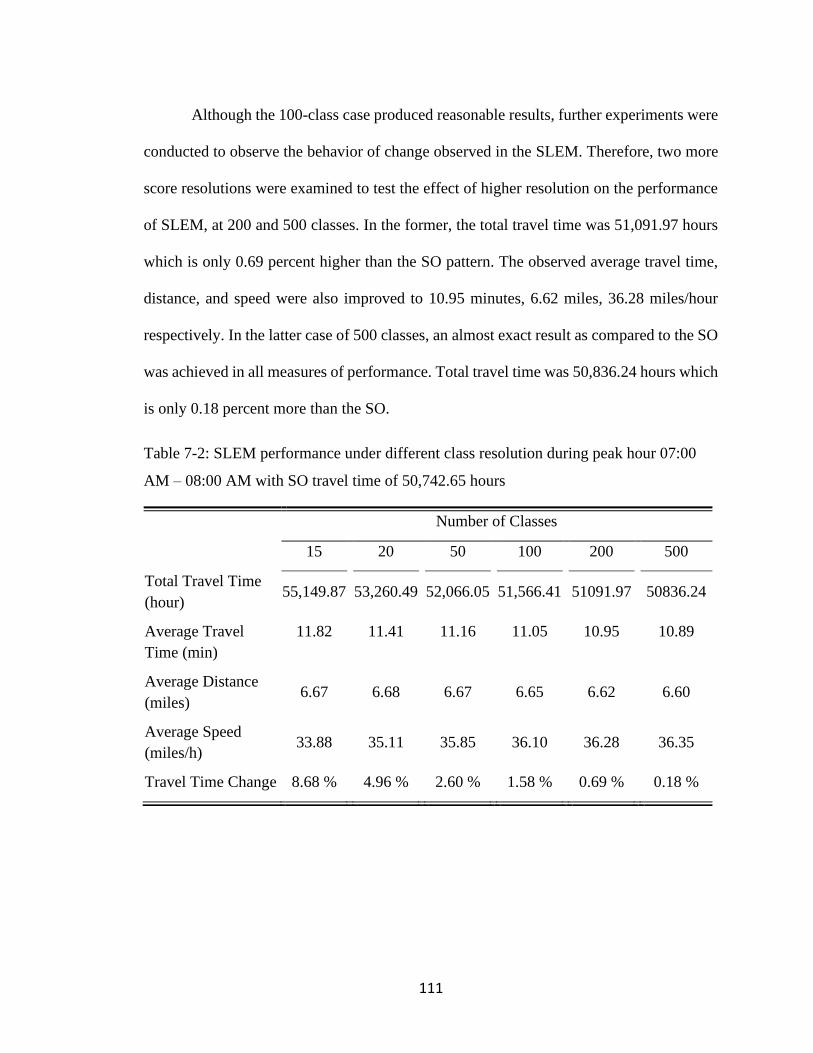
111
Although the 100-class case produced reasonable results, further experiments were
conducted to observe the behavior of change observed in the SLEM. Therefore, two more
score resolutions were examined to test the effect of higher resolution on the performance
of SLEM, at 200 and 500 classes. In the former, the total travel time was 51,091.97 hours
which is only 0.69 percent higher than the SO pattern. The observed average travel time,
distance, and speed were also improved to 10.95 minutes, 6.62 miles, 36.28 miles/hour
respectively. In the latter case of 500 classes, an almost exact result as compared to the SO
was achieved in all measures of performance. Total travel time was 50,836.24 hours which
is only 0.18 percent more than the SO.
Table 7-2: SLEM performance under different class resolution during peak hour 07:00
AM – 08:00 AM with SO travel time of 50,742.65 hours
Number of Classes
15 20 50 100 200 500
Total Travel Time
(hour) 55,149.87 53,260.49 52,066.05 51,566.41 51091.97 50836.24
Average Travel
Time (min)
11.82 11.41 11.16 11.05 10.95 10.89
Average Distance
(miles) 6.67 6.68 6.67 6.65 6.62 6.60
Average Speed
(miles/h) 33.88 35.11 35.85 36.10 36.28 36.35
Travel Time Change 8.68 % 4.96 % 2.60 % 1.58 % 0.69 % 0.18 %

112
Figure 7-3: Network performance given scoring systems having different resolutions
7-5. Route Assignment Pattern Comparison
This experiment aims to test the driver score relationship with the level of demand
assuming the scores are distributed among 100 classes. Given different demand levels, the
minimum score to access major highways was assumed to change with respect to the
demand level, such that when demand is low the low-performance drivers would have a
higher chance to access their preferred routes. Besides, the SO and SLEM traffic
assignment would also have no superior performance over the UE traffic assignment.
Figure 7-4 shows a 24-hour demand volume of the testbed network where four different
time periods were chosen to conduct this experiment.
15 Classes
20 Classes
50 Classes
100 Classes
200 Classes500 Classes
SO Travel Time
50,700
51,200
51,700
52,200
52,700
53,200
53,700
54,200
54,700
55,200
Tota
l T
raver
Tim
e (H
ours
)
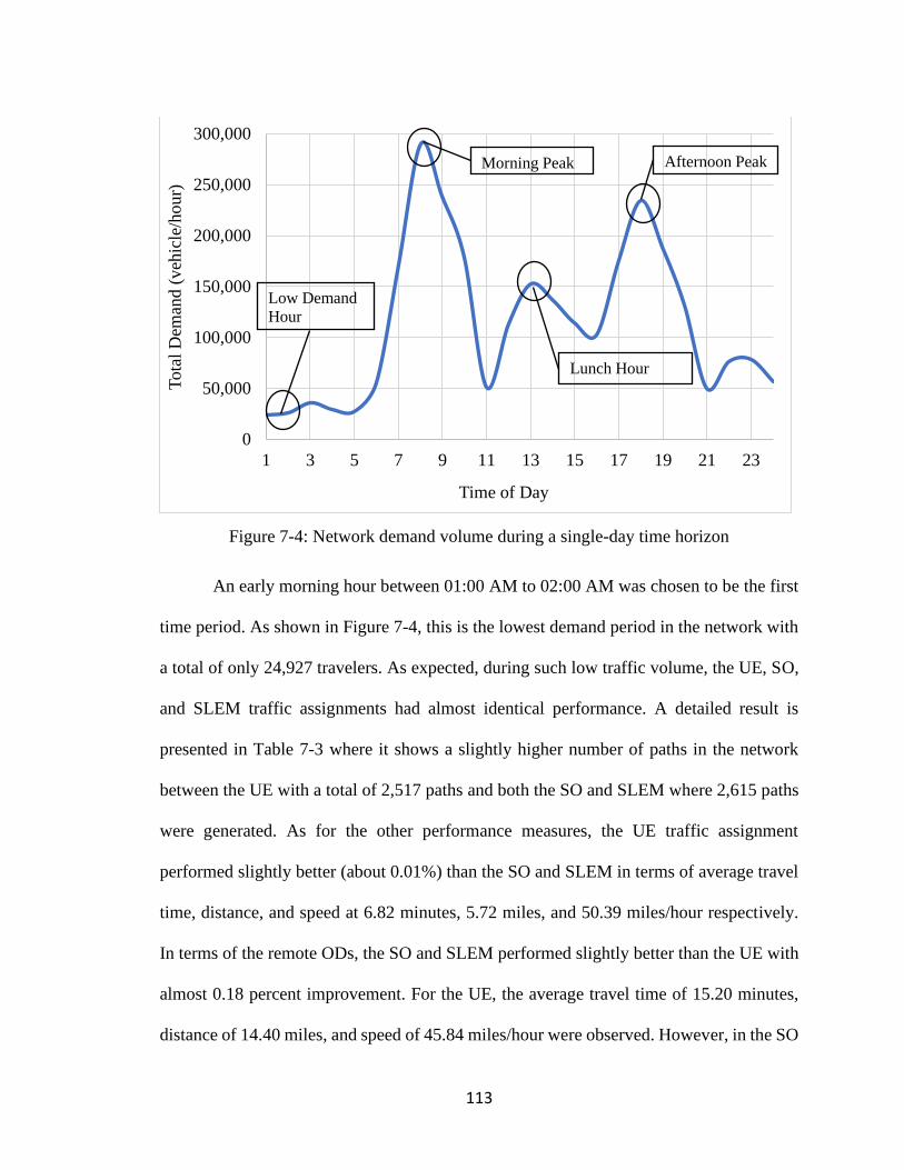
113
ddd
Figure 7-4: Network demand volume during a single-day time horizon
An early morning hour between 01:00 AM to 02:00 AM was chosen to be the first
time period. As shown in Figure 7-4, this is the lowest demand period in the network with
a total of only 24,927 travelers. As expected, during such low traffic volume, the UE, SO,
and SLEM traffic assignments had almost identical performance. A detailed result is
presented in Table 7-3 where it shows a slightly higher number of paths in the network
between the UE with a total of 2,517 paths and both the SO and SLEM where 2,615 paths
were generated. As for the other performance measures, the UE traffic assignment
performed slightly better (about 0.01%) than the SO and SLEM in terms of average travel
time, distance, and speed at 6.82 minutes, 5.72 miles, and 50.39 miles/hour respectively.
In terms of the remote ODs, the SO and SLEM performed slightly better than the UE with
almost 0.18 percent improvement. For the UE, the average travel time of 15.20 minutes,
distance of 14.40 miles, and speed of 45.84 miles/hour were observed. However, in the SO
0
50,000
100,000
150,000
200,000
250,000
300,000
1 3 5 7 9 11 13 15 17 19 21 23
Tota
l D
eman
d (
veh
icle
/hour)
Time of Day
Morning Peak
Low Demand
Hour
Lunch Hour
Afternoon Peak
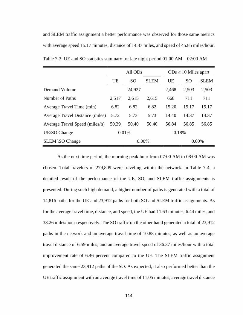
114
and SLEM traffic assignment a better performance was observed for those same metrics
with average speed 15.17 minutes, distance of 14.37 miles, and speed of 45.85 miles/hour.
Table 7-3: UE and SO statistics summary for late night period 01:00 AM – 02:00 AM
All ODs ODs ≥ 10 Miles apart
UE SO SLEM
UE
SO
SLEM
Demand Volume 24,927 2,468 2,503 2,503
Number of Paths 2,517 2,615 2,615 668 711 711
Average Travel Time (min) 6.82 6.82 6.82 15.20 15.17 15.17
Average Travel Distance (miles) 5.72 5.73 5.73 14.40 14.37 14.37
Average Travel Speed (miles/h) 50.39 50.40 50.40 56.84 56.85 56.85
UE/SO Change 0.01% 0.18%
SLEM \SO Change 0.00% 0.00%
As the next time period, the morning peak hour from 07:00 AM to 08:00 AM was
chosen. Total travelers of 279,809 were traveling within the network. In Table 7-4, a
detailed result of the performance of the UE, SO, and SLEM traffic assignments is
presented. During such high demand, a higher number of paths is generated with a total of
14,816 paths for the UE and 23,912 paths for both SO and SLEM traffic assignments. As
for the average travel time, distance, and speed, the UE had 11.63 minutes, 6.44 miles, and
33.26 miles/hour respectively. The SO traffic on the other hand generated a total of 23,912
paths in the network and an average travel time of 10.88 minutes, as well as an average
travel distance of 6.59 miles, and an average travel speed of 36.37 miles/hour with a total
improvement rate of 6.46 percent compared to the UE. The SLEM traffic assignment
generated the same 23,912 paths of the SO. As expected, it also performed better than the
UE traffic assignment with an average travel time of 11.05 minutes, average travel distance
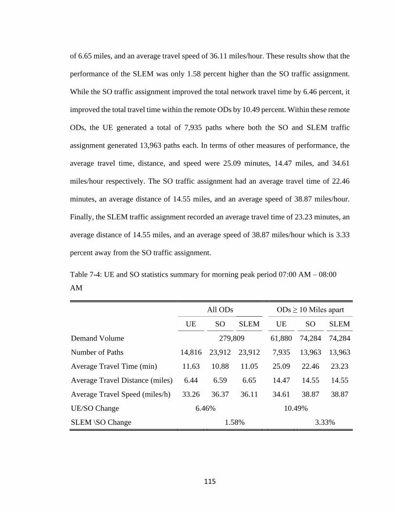
115
of 6.65 miles, and an average travel speed of 36.11 miles/hour. These results show that the
performance of the SLEM was only 1.58 percent higher than the SO traffic assignment.
While the SO traffic assignment improved the total network travel time by 6.46 percent, it
improved the total travel time within the remote ODs by 10.49 percent. Within these remote
ODs, the UE generated a total of 7,935 paths where both the SO and SLEM traffic
assignment generated 13,963 paths each. In terms of other measures of performance, the
average travel time, distance, and speed were 25.09 minutes, 14.47 miles, and 34.61
miles/hour respectively. The SO traffic assignment had an average travel time of 22.46
minutes, an average distance of 14.55 miles, and an average speed of 38.87 miles/hour.
Finally, the SLEM traffic assignment recorded an average travel time of 23.23 minutes, an
average distance of 14.55 miles, and an average speed of 38.87 miles/hour which is 3.33
percent away from the SO traffic assignment.
Table 7-4: UE and SO statistics summary for morning peak period 07:00 AM – 08:00
AM
All ODs ODs ≥ 10 Miles apart
UE SO SLEM
UE
SO
SLEM
Demand Volume 279,809 61,880 74,284 74,284
Number of Paths 14,816 23,912 23,912 7,935 13,963 13,963
Average Travel Time (min) 11.63 10.88 11.05 25.09 22.46 23.23
Average Travel Distance (miles) 6.44 6.59 6.65 14.47 14.55 14.55
Average Travel Speed (miles/h) 33.26 36.37 36.11 34.61 38.87 38.87
UE/SO Change 6.46% 10.49%
SLEM \SO Change 1.58% 3.33%

116
Another period examined was the lunch break hour between 12:00 PM to 13:00
PM. During this one hour, the total number in the network was 148,703 travelers. As shown
in Table 7-5, the UE traffic assignment produced a total of 6,371 paths within the network
and had an average travel time of 8.46 minutes, an average distance of 6.28 miles, and an
average speed of 44.52 miles/hour. The SO traffic assignment on the other hand improved
the network performance under the UE traffic assignment by 2.07 percent where the
average travel time, distance, and speed were 8.29 minutes, 6.25 miles, and 45.27
miles/hour respectively. Additionally, the SLEM traffic assignment produced not only the
same number of paths produced under the SO traffic assignment, but also almost identical
overall performance with only a 0.13 percent difference, where the average travel time,
distance, and speed were 8.29 minutes, 6.25 miles, and 45.24 miles/hour respectively. The
remote ODs produced a better performance for the SO and SLEM traffic assignments
compared to the UE traffic assignment, where 2,592 paths were produced in the latter
versus 4,552 in both SO and SLEM. Under the UE traffic assignment, the average travel
time was 17.72 minutes, distance was 14.13 miles, and speed was 47.83 miles/hour. The
SO traffic assignment improved travel by 4.30 percent with an average travel time of 16.96
minutes, an average distance of 14.16 miles, and an average speed of 50.08 miles/hour.
Surprisingly, the SLEM performance was the same as the SO traffic assignment in terms
of the average travel distance and speed of 14.16 miles and 50.08 miles/hour respectively.
As for the travel time, the system under the SLEM had an average trip time of 17.02
minutes, which is only 0.34 percent away from the SO.
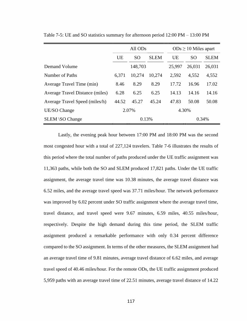
117
Table 7-5: UE and SO statistics summary for afternoon period 12:00 PM – 13:00 PM
All ODs ODs ≥ 10 Miles apart
UE SO SLEM
UE
SO
SLEM
Demand Volume 148,703 25,997 26,031 26,031
Number of Paths 6,371 10,274 10,274 2,592 4,552 4,552
Average Travel Time (min) 8.46 8.29 8.29 17.72 16.96 17.02
Average Travel Distance (miles) 6.28 6.25 6.25 14.13 14.16 14.16
Average Travel Speed (miles/h) 44.52 45.27 45.24 47.83 50.08 50.08
UE/SO Change 2.07% 4.30%
SLEM \SO Change 0.13% 0.34%
Lastly, the evening peak hour between 17:00 PM and 18:00 PM was the second
most congested hour with a total of 227,124 travelers. Table 7-6 illustrates the results of
this period where the total number of paths produced under the UE traffic assignment was
11,363 paths, while both the SO and SLEM produced 17,821 paths. Under the UE traffic
assignment, the average travel time was 10.38 minutes, the average travel distance was
6.52 miles, and the average travel speed was 37.71 miles/hour. The network performance
was improved by 6.02 percent under SO traffic assignment where the average travel time,
travel distance, and travel speed were 9.67 minutes, 6.59 miles, 40.55 miles/hour,
respectively. Despite the high demand during this time period, the SLEM traffic
assignment produced a remarkable performance with only 0.34 percent difference
compared to the SO assignment. In terms of the other measures, the SLEM assignment had
an average travel time of 9.81 minutes, average travel distance of 6.62 miles, and average
travel speed of 40.46 miles/hour. For the remote ODs, the UE traffic assignment produced
5,959 paths with an average travel time of 22.51 minutes, average travel distance of 14.22

118
miles, and average travel speed of 37.90 miles/hour. A significant improvement in the
network performance was achieved under the SO traffic assignment which reached 10.34
percent compared to the UE traffic assignment. With a total of 9,934 paths, the SO had an
average travel time, average travel distance, and average travel speed of 20.18 minutes,
14.35 miles, and 42.65 miles/hour respectively. The SLEM also produced a promising
result within the remote ODs with only 0.70 percent variance from the SO. The SLEM also
had the same number of paths as the SO and had an average travel time of 20.39 minutes,
average travel distance of 14.45 miles, and average travel speed of 42.52 miles/hour.
Table 7-6: UE and SO statistics summary for evening peak period 17:00 PM – 18:00 PM
All ODs ODs ≥ 10 Miles apart
UE SO SLEM
UE
SO
SLEM
Demand Volume 227,124 48,363 49,541 49,541
Number of Paths 11,363 17,821 17,821 5,959 9,934 9,934
Average Travel Time (min) 10.38 9.76 9.81 22.51 20.18 20.39
Average Travel Distance (miles) 6.52 6.59 6.62 14.22 14.35 14.45
Average Travel Speed (miles/h) 37.71 40.55 40.46 37.90 42.65 42.52
UE/SO Change 6.02% 10.34%
SLEM\SO Change 0.34% 0.70%
To further investigate the score changing, two remote ODs were picked to illustrate
the experiment in order to achieve a deeper understanding of the SLEM performance
compared to the UE and SO. Figure 7-5 shows the map of the city of Dallas, TX, and the
two ODs. The first OD (in red) is over 16 miles long and located on US-75 where it starts
from the southern part of the highway near the downtown and ends up in the northern part
of the highway in Plano, TX. The second OD (in blue) is about 13 miles long where it starts
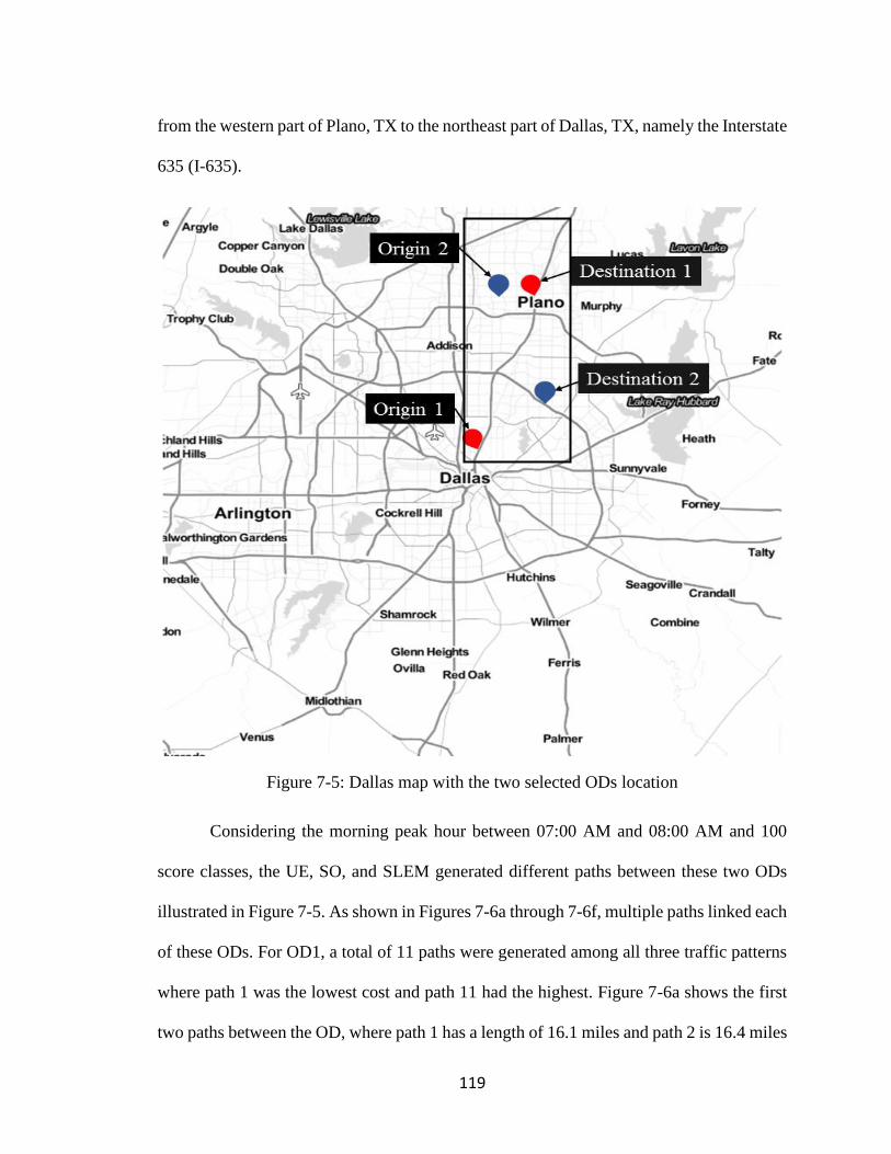
119
from the western part of Plano, TX to the northeast part of Dallas, TX, namely the Interstate
635 (I-635).
Figure 7-5: Dallas map with the two selected ODs location
Considering the morning peak hour between 07:00 AM and 08:00 AM and 100
score classes, the UE, SO, and SLEM generated different paths between these two ODs
illustrated in Figure 7-5. As shown in Figures 7-6a through 7-6f, multiple paths linked each
of these ODs. For OD1, a total of 11 paths were generated among all three traffic patterns
where path 1 was the lowest cost and path 11 had the highest. Figure 7-6a shows the first
two paths between the OD, where path 1 has a length of 16.1 miles and path 2 is 16.4 miles

120
long. Both path 1 and 2 overlap the majority of their lengths on the US-75 except for the
last small part where they differ as shown in the zoomed-in upper-left corner. Paths 3 to 5
are shown in Figure 7-6b where they differ from the first two and are slightly longer where
their lengths are 16.6, 17.3, and 17.2 miles respectively. Path 3 travels primarily on US-75
where it eventually diverges toward the eastern side arterial. Both paths 4 and 5 have major
divergences to the west side US-75 arterials. Figure 7-6c illustrates paths 6, 7, and 8, which
have lengths of 17.5, 16.6, and 16.9 miles, respectively. Path 6 is the longest among all 11
paths, diverging west as do both paths 4 and 5. As for 7, it has frequent link turns which
shape the zigzag characteristics of that path. Path 8 on the other hand has the majority of
its length on the eastern parallel arterial to the US-75. Figure 7-6d shows the last three
paths 9, 10, and 11 which are 16.9, 17.2, and 16.9 miles long respectively. Path 9 shares
similarities with both paths 1 and 2 where it has the majority of its links on the US-75 and
only differs in the last few miles to the destination. Both paths 10 and 11 have major parts
of their length on the US-75 but diverge from it on other parts.
For OD2, a total of six different paths were generated between the origin in Plano,
TX to the destination in northeast Dallas, TX such that path 1 is the lowest cost path and
path 6 is the highest cost. Paths 1, 2, and 3 are shown in Figure 7-6e where their lengths
are 12.8, 14, and 13.4 miles respectively. Path 1 has most of its length on a major arterial
on the south direction and I-635 on the east direction. Similarly, path 2 has the southern
direction on a minor road where it shares path 1’s eastern direction on I-635 highway. Path
3 on the other hand does not share the characteristics of the first two paths. In fact, it is
constructed of multiple minor and major roads. Paths 4 through 6 are illustrated in Figure
7-6f where they are 19.9, 12.9, and 14 miles long. Path 4 has minor roads on the southern

121
direction and then the I-635 on the eastern direction. Path 5 has a different characteristic
where it is mostly constructed of minor roads in different directions. Path 6 has the majority
of the south direction constructed of minor roads and I-635 to the east direction.
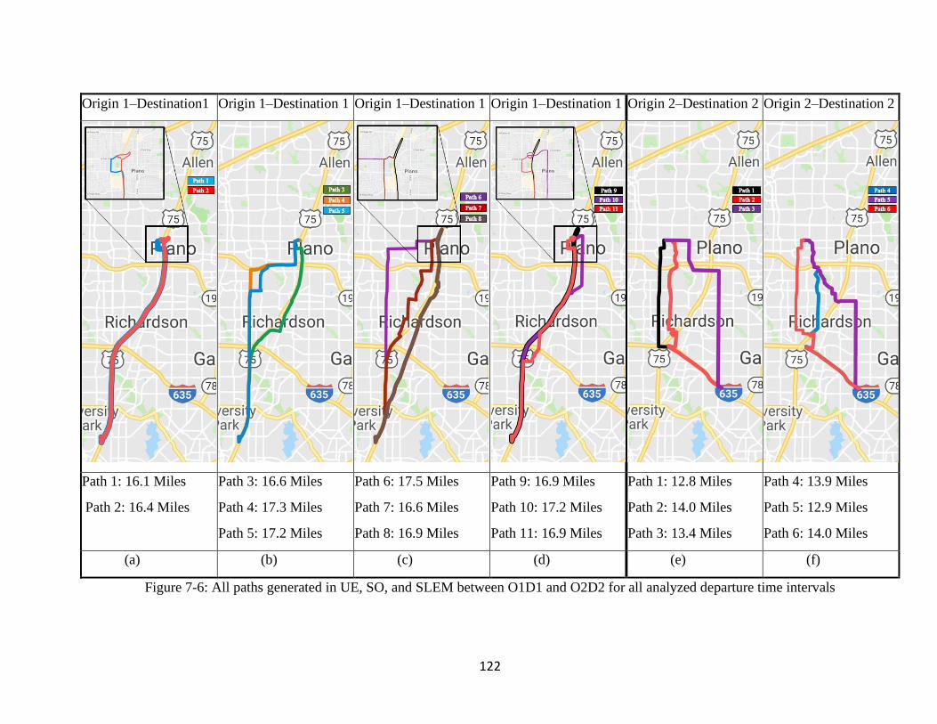
122
Origin 1–Destination1 Origin 1–Destination 1 Origin 1–Destination 1 Origin 1–Destination 1 Origin 2–Destination 2 Origin 2–Destination 2
Path 1: 16.1 Miles
Path 2: 16.4 Miles
Path 3: 16.6 Miles
Path 4: 17.3 Miles
Path 5: 17.2 Miles
Path 6: 17.5 Miles
Path 7: 16.6 Miles
Path 8: 16.9 Miles
Path 9: 16.9 Miles
Path 10: 17.2 Miles
Path 11: 16.9 Miles
Path 1: 12.8 Miles
Path 2: 14.0 Miles
Path 3: 13.4 Miles
Path 4: 13.9 Miles
Path 5: 12.9 Miles
Path 6: 14.0 Miles
(a) (b) (c) (d) (e) (f)
Figure 7-6: All paths generated in UE, SO, and SLEM between O1D1 and O2D2 for all analyzed departure time intervals

123
To further investigate the score, change, and how the SLEM traffic assignments
perform compared to both UE and SO traffic assignment patterns, the results extracted of
the two remote ODs are visualized in Figure 7-6 during each of the four time periods
reported in Tables 7-3 through 7-6. The objective of this experiment is to observe the
change of score and how the score reacts to the level of demand. For each OD, the UE, SO
and the SLEM traffic assignments were compared based on the used routes and the
percentage of assigned travelers for each path. Figure 7-7 shows the difference in the
assignment split among all three traffic patterns for both ODs. In OD1, Figures 7-7
illustrates the demand split of the UE, SO, and SLEM for each period evaluated, as well as
the split of the demand among the different paths generated between each OD as show in
Figure 7-6.
Figures 7-7a-d illustrate the OD1 demand split over time. For the first time period
of 01:00 AM - 02:00 AM results are as expected. As shown in Figure 7-7a, a similar split
pattern was produced among all three traffic assignment patterns UE, SO, and SLEM in
terms of the traffic assignment weight of each path due to the low demand level.
When the demand is high during the 07:00 AM – 08:00 AM period as shown in
Figure 7-7b and Table 7-7, a different split among all 8 paths are occurs. For the UE traffic
assignment, the majority of travelers (98.44 percent) were assigned to the first path where
the remaining 1.56 percent were assigned to the second path. As for the SO traffic
assignment, the travelers were assigned to the first eight paths with different weights. As
shown inTable7-7, the majority of 81.47 percent of travelers were assigned to path 1. The
rest of (18.53 percent) were assigned as follows: 7.41 percent were assigned to path 7, 3.70
percent were assigned to path 2, 2.78 percent were assigned to path 5, 1.85 percent were
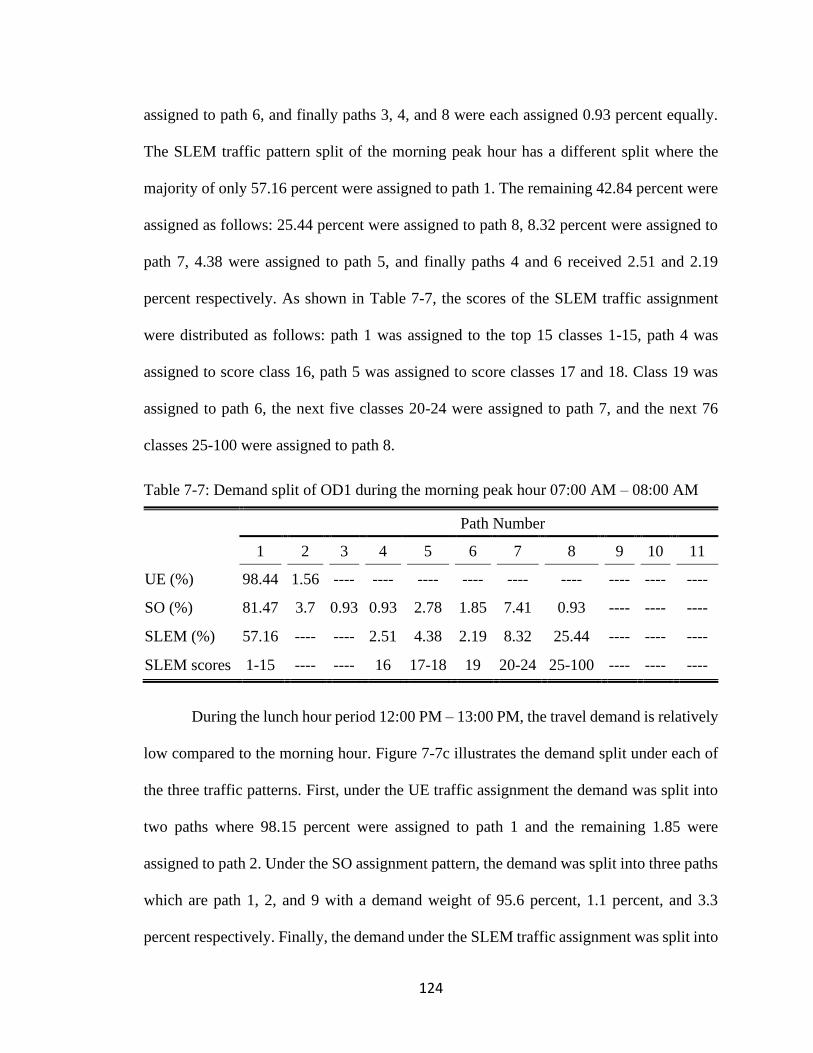
124
assigned to path 6, and finally paths 3, 4, and 8 were each assigned 0.93 percent equally.
The SLEM traffic pattern split of the morning peak hour has a different split where the
majority of only 57.16 percent were assigned to path 1. The remaining 42.84 percent were
assigned as follows: 25.44 percent were assigned to path 8, 8.32 percent were assigned to
path 7, 4.38 were assigned to path 5, and finally paths 4 and 6 received 2.51 and 2.19
percent respectively. As shown in Table 7-7, the scores of the SLEM traffic assignment
were distributed as follows: path 1 was assigned to the top 15 classes 1-15, path 4 was
assigned to score class 16, path 5 was assigned to score classes 17 and 18. Class 19 was
assigned to path 6, the next five classes 20-24 were assigned to path 7, and the next 76
classes 25-100 were assigned to path 8.
Table 7-7: Demand split of OD1 during the morning peak hour 07:00 AM – 08:00 AM
Path Number
1 2 3 4 5 6 7 8 9 10 11
UE (%) 98.44 1.56 ---- ---- ---- ---- ---- ---- ---- ---- ----
SO (%) 81.47 3.7 0.93 0.93 2.78 1.85 7.41 0.93 ---- ---- ----
SLEM (%) 57.16 ---- ---- 2.51 4.38 2.19 8.32 25.44 ---- ---- ----
SLEM scores 1-15 ---- ---- 16 17-18 19 20-24 25-100 ---- ---- ----
During the lunch hour period 12:00 PM – 13:00 PM, the travel demand is relatively
low compared to the morning hour. Figure 7-7c illustrates the demand split under each of
the three traffic patterns. First, under the UE traffic assignment the demand was split into
two paths where 98.15 percent were assigned to path 1 and the remaining 1.85 were
assigned to path 2. Under the SO assignment pattern, the demand was split into three paths
which are path 1, 2, and 9 with a demand weight of 95.6 percent, 1.1 percent, and 3.3
percent respectively. Finally, the demand under the SLEM traffic assignment was split into

125
two paths. The majority of 91.23 percent of the demand was assigned to path 1 which
included the score classes 1 - 41. The remaining 8.77 percent of the demand was assigned
to path 9 with the score classes from 42-100.
The evening peak hour period from 17:00 PM to 18:00 PM is the second-highest
congested hour to be considered. Under the UE traffic assignment, the demand was split
into three paths. As shown in Table 7-8, the majority of demand of 97.83 percent was
assigned to path 1 where the remaining 2.17 percent were assigned to paths 9 and 10 with
1.45 percent and 0.72 percent respectively. Under the SO pattern, the demand was split
into five different paths where the majority of 94.4 percent were assigned to path 1. Both
paths 2 and 11 were assigned 1.87 percent and both paths 9 and 10 received 0.93 percent
of the demand. The SLEM assignment generated three paths during this hour. The majority
of 74.57 percent of demand was assigned to path 1 which includes the score classes of 1-
24. Score class 25 which weighs 1.46 percent was assigned to path 9. Finally, path 10 was
the second busiest path under the SLEM traffic pattern with 23.97 percent of the demand,
which included score classes 26-100.
Table 7-8: Demand split of OD1 during the evening peak hour 17:00 PM – 18:00 PM
Path Number
1 2 3 4 5 6 7 8 9 10 11
UE (%) 97.83 ---- ---- ---- ---- ---- ---- ---- 1.45 0.72 ----
SO (%) 94.4 1.87 ---- ---- ---- ---- ---- ---- 0.93 0.93 1.87
SLEM (%) 74.57 ---- ---- ---- ---- ---- ---- ---- 1.46 23.97 ----
SLEM scores 1-24 ---- ---- ---- ---- ---- ---- ---- 25 26-100 ----

126
The second OD to examine (OD2) has a total of 6 paths as shown in figure 7-6, and
their detailed demand split is illustrated in figures 7-7e through 7-7h below. Choosing the
same four demand intervals as the OD1, a similar result was obtained for the early morning
hour between 01:00 AM to 02:00 AM where the three traffic assignment patterns were
exactly the same and no split was observed as illustrated in Figure 7-7e.
As expected, during the morning peak hour 07:00 AM – 08:00 AM, a demand split
was observed within all three traffic assignment patterns as shown in Figure 7-7f and Table
7-9. Under the UE, the traffic between this OD was split into three paths: 98.44 percent of
travelers were assigned to path 1 and the remaining 1.56 percent were divided equally into
path 3 and path 4, with 0.78 percent each. When the SO traffic assignment was considered,
the demand between this OD was split into five different paths. As expected, path 1 had
the majority of 96.28 percent of the total demand, where the remaining 3.72 percent was
distributed equally among paths 2-5 with 0.93 percent each. Under the SLEM assignment,
the demand between this OD was distributed among three paths. Path 1 also had the
majority of 74.57 (score classes 1-24), which is considerably less compared to the UE and
SO. The remaining 25.43 percent where assigned as follows: 1.46 percent (score class 25)
was assigned to path 2 and 23.97 percent (score classes 26-100) was assigned to path 5.
Table 7-9: Demand split of OD2 during the morning peak hour 07:00 AM – 08:00 AM
Path Number
1 2 3 4 5 6
UE (%) 98.44 ---- 0.78 0.78 ---- ----
SO (%) 96.28 0.93 0.93 0.93 0.93 ----
SLEM (%) 74.57 1.46 ---- ---- 23.97 ----
SLEM scores 1-24 25 ---- ---- 26-100 ----

127
During the lunch hour break from 12:00 PM to 13:00 PM, the demand split between
OD2 did not occur across all three traffic assignments. As shown in Figure 7-7g, the UE,
SO, and the SLEM all had similar patterns where all demand was assigned to path 1, which
indicates a low demand.
Figure 7-7h shows the demand split pattern between OD2 during the evening peak
hour from 17:00 PM to 18:00 PM and the detailed percentages are reported in Table 7-10.
Under the UE traffic assignment, all travelers were assigned to path 1 and surprisingly, no
path split was observed. When SO traffic assignment was implemented, the OD2 demand
was split into two paths where the majority of travelers were assigned to path 1 with 99.07
percent, and only 0.93 percent of travelers were assigned to path 6, which is the least. A
demand split was also observed under the SLEM traffic pattern. Similar to the SO, the split
occurred on paths 1 and 6 with the majority of travelers (91.71) percent assigned to path 1,
which includes score classes 1-42. The remaining 8.29 percent (score classes 43-100) was
assigned to path 6.
Table 7-10: Demand split of OD2 during the evening peak hour 17:00 PM – 18:00 PM
Path Number
1 2 3 4 5 6
UE (%) 100 ---- ---- ---- ---- ----
SO (%) 99.07 ---- ---- ---- ---- 0.93
SLEM (%) 91.71 ---- ---- ---- ---- 8.29
SLEM scores 1-42 ---- ---- ---- ---- 43-100

128
OD1 OD2
01:0
0 A
M -
02:0
0 A
M
(a) (e)
07:0
0 A
M -
08:0
0 A
M
(b) (f)
12:0
0 P
M -
13:0
0 P
M
(c) (g)
17:0
0 P
M -
18:0
0 P
M
(d) (h)
Figure 7-7: Detailed distribution of the selected remote ODs
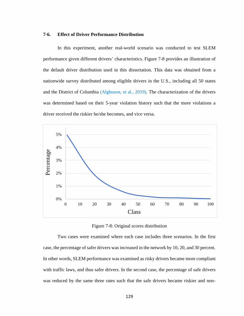
129
7-6. Effect of Driver Performance Distribution
In this experiment, another real-world scenario was conducted to test SLEM
performance given different drivers’ characteristics. Figure 7-8 provides an illustration of
the default driver distribution used in this dissertation. This data was obtained from a
nationwide survey distributed among eligible drivers in the U.S., including all 50 states
and the District of Columbia (Alghuson, et al., 2019). The characterization of the drivers
was determined based on their 5-year violation history such that the more violations a
driver received the riskier he/she becomes, and vice versa.
Figure 7-8: Original scores distribution
Two cases were examined where each case includes three scenarios. In the first
case, the percentage of safer drivers was increased in the network by 10, 20, and 30 percent.
In other words, SLEM performance was examined as risky drivers became more compliant
with traffic laws, and thus safer drivers. In the second case, the percentage of safe drivers
was reduced by the same three rates such that the safe drivers became riskier and non-
0%
1%
2%
3%
4%
5%
0 10 20 30 40 50 60 70 80 90 100
Per
cen
tage
Class
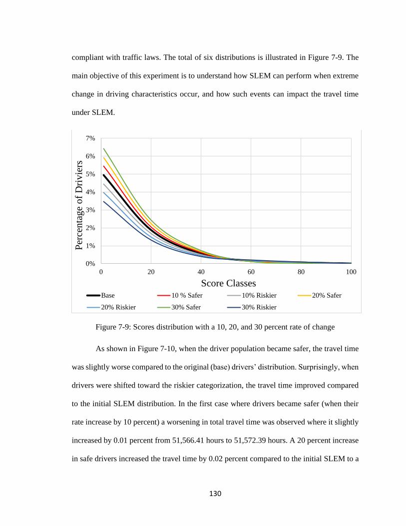
130
compliant with traffic laws. The total of six distributions is illustrated in Figure 7-9. The
main objective of this experiment is to understand how SLEM can perform when extreme
change in driving characteristics occur, and how such events can impact the travel time
under SLEM.
Figure 7-9: Scores distribution with a 10, 20, and 30 percent rate of change
As shown in Figure 7-10, when the driver population became safer, the travel time
was slightly worse compared to the original (base) drivers’ distribution. Surprisingly, when
drivers were shifted toward the riskier categorization, the travel time improved compared
to the initial SLEM distribution. In the first case where drivers became safer (when their
rate increase by 10 percent) a worsening in total travel time was observed where it slightly
increased by 0.01 percent from 51,566.41 hours to 51,572.39 hours. A 20 percent increase
in safe drivers increased the travel time by 0.02 percent compared to the initial SLEM to a
0%
1%
2%
3%
4%
5%
6%
7%
0 20 40 60 80 100
Per
cen
tag
e o
f D
riv
iers
Score ClassesBase 10 % Safer 10% Riskier 20% Safer
20% Riskier 30% Safer 30% Riskier

131
total of 51,578.29 hours. When the safe drivers increased to 30 percent, the total network
travel time increased 0.07 percent (51,604.61 hours). In case 2, when the safe drivers were
reduced by 10 percent, the total network travel time did not change. A 20 percent reduction
in safe drivers resulted in a 0.03 percent improvement in total network travel time which
reached 51,552.22 hours compared to the initial SLEM total travel time of 51,566.41 hours.
When safe drivers were reduced by 30 percent, the total network travel time was also
reduced by 0.05 percent which is equivalent to 51,540.97 hours. A possible explanation of
this result is that the reduction in safer drivers led to a decrease in the size of classes for
safer drivers, which resulted in a reduced number of drivers competing for the best route,
and thus SLEM had more freedom to distribute drivers to higher cost paths.
Figure 7-10: Total travel time change under different distributions
Base SLEM
Travel Time
+10% Safe
+20% Safe
+30% Safe
+10% Risky
+20% Risky
+30% Risky
51,540
51,550
51,560
51,570
51,580
51,590
51,600
51,610
Tota
l T
ravel
Tim
e (H
ours
)
Safe Drivers Risky Drivers

132
While the total network performance is illustrated above, detailed average
performance metrics are reported in Table 7-11. When safer and risky drivers increased by
10, 20, and 30 percent, the average network travel time, distance, and speed were almost
the same for both as compared to the initial SLEM at 11.05 minutes 6.65 miles, and 36.11
miles/hour respectively. When the same metrics were applied to the remote ODs, no
significant change was noticed in the average travel time compared to the SLEM. However,
increasing both the safer and risky drivers by 10, 20, and 30 percent increased the average
travel distance along all six distributions by almost 2 percent, from 14.55 minutes under
initial SLEM to 14.84. As for the average travel speed, although no significant changes
were observed among all six distributions, one can conclude that the increasing rate of
risky drivers slightly increased the average speed, which could be explained by the fact
that the punishment was more severe on more drivers, also resulting in an increase of the
average distance.
Table 7-11: Summary for different class distributions during the morning peak hour
07:00 AM – 08:00 AM
Initial
SLEM
Safer Drivers Risky Drivers
For all ODs
+10% +20% +30%
+10% +20% +30%
Average Travel Time (minutes) 11.05 11.06 11.06 11.07 11.06 11.05 11.05
Average Travel Distance (miles) 6.65 6.65 6.65 6.66 6.65 6.66 6.65
Average Travel Speed (miles/h) 36.11 36.10 36.10 36.09 36.11 36.13 36.12
For Remote ODs
Average Travel Time (minutes) 23.23 23.25 23.24 23.26 23.24 23.24 23.23
Average Travel Distance (miles) 14.55 14.84 14.84 14.84 14.84 14.85 14.85
Average Travel Speed (miles/h) 38.87 38.85 38.86 38.84 38.86 38.90 38.90

133
7-7. SLEM Performance Under Different Compliance Scenarios
Another real-world scenario is conducted in this section where a non-compliant
behavior from certain drivers is considered. Five different ratios of non-compliance were
considered where they ranged from as low as 5 percent (95 percent compliance rate) to a
severe scenario of 25 percent (75 percent compliance rate). As illustrated in Figure 7-11,
the initial total network travel time under SLEM was 51,566.41 hours and a one-percent
non-compliance had no impact on the total travel time. When the non-compliance rate was
increased to 5 percent, the total travel time increased by 0.78 percent to reach 51,947.57
hours. Next, the noncompliance rate increased by 5 percent in steps of 10, 15, 20, and 25
percent, and the total network travel time worsened to 52,264.60 hours (1.35 percent),
52,678.13 hours (2.15 percent), 53,026.54 hours (2.83 percent), and 53,808.13 hours (4.34
percent) respectively.
Figure 7-11: Non-compliance impact on total network travel time
50,500
51,000
51,500
52,000
52,500
53,000
53,500
54,000
54,500
0% 5% 10% 15% 20% 25%
Tota
l N
etw
ork
Tra
vel
Tim
e (H
ours
)
Percentage of non-compliant drivers
SLEM SO UE

134
A detailed result is reported in Table 7-12 where the impact of the different non-
compliance rates on other network performance metrics was compared. When non-
compliance rate was increased by 1, 5, 10, 15, 20, and 25 percent, the average network
travel time increased from 11.05 minutes by 0.18, 0.81, 1.45, 2.26, 2.90, and 4.43 percent
respectively. The average network travel distance also increased from the initial 6.65 miles
by 0.15, 0.3, 0.45, 0.75, 0.90, and 1.2 percent respectively. Similarly, the average network
travel speed was also worsened by 0.06, 0.47, 0.91, 1.47, 1.94, and 3.07 percent
respectively from its initial average speed of 36.11 miles/hour. While the impact on the
whole network was not significant, the same non-compliance rates had a more significant
impact on the remote ODs. As shown in Table 7-12, the average travel time increased from
23.23 minutes initially by 0.22, 1.46, 2.67, 3.75, 4.95, and 7.4 percent respectively. The
average travel distance also increased from its initial 14.55 miles by 2.13, 2.89, 3.51, 3.78,
4.12, and 4.81 percent respectively. Finally, the average travel speed also worsened from
the initial average speed of 38.87 by 1.47, 1.93, 2.55, 3.29, 4.06, and 5.66 percent
respectively.

135
Table 7-12: Results summary for non-compliance impact on network performance.
7-8. SLEM Performance Under Non-Recurrent Incident
In this experiment, the performance of SLEM’s route guidance strategy under non-
recurrent congestion situations is evaluated. In the morning peak hour, incidents frequently
occur on the southbound direction upstream of the interchange with I-635, as illustrated in
Figure 7-12. Among the 4-lanes, three different lane closure scenarios were considered: 1
lane (25 percent), 2 lanes (50 percent), and 3 lanes (75 percent). Two cases were considered
for each incident scenario. In the first case, SLEM’s route guidance strategy obtained for
the no-incident scenario was applied, representing a situation in which the incident
information was not communicated to SLEM. In the second case, the incident information
was communicated to SLEM, which generated an updated route guidance strategy that
captured the congestion caused by the incident.
Non-Compliance Rate
For all ODs Initial 1% 5% 10% 15% 20% 25%
Average Travel Time (minutes) 11.05 11.07 11.14 11.21 11.3 11.37 11.54
Average Travel Distance (miles) 6.65 6.66 6.67 6.68 6.70 6.71 6.73
Average Travel Speed (miles/h) 36.11 36.09 35.94 35.78 35.58 35.41 35.00
For Remote ODs
Average Travel Time (minutes) 23.23 23.28 23.57 23.85 24.1 24.38 24.95
Average Travel Distance (miles) 14.55 14.86 14.97 15.06 15.1 15.15 15.25
Average Travel Speed (miles/h) 38.87 38.3 38.12 37.88 37.59 37.29 36.67
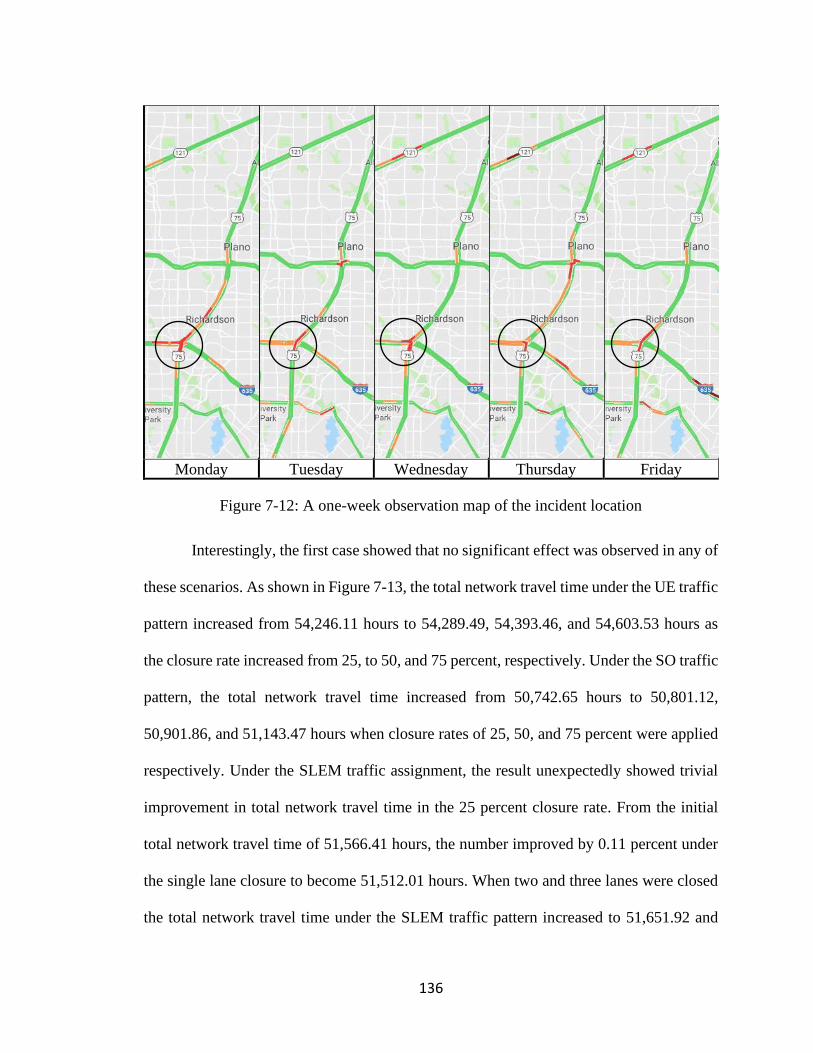
136
Monday Tuesday Wednesday Thursday Friday
Figure 7-12: A one-week observation map of the incident location
Interestingly, the first case showed that no significant effect was observed in any of
these scenarios. As shown in Figure 7-13, the total network travel time under the UE traffic
pattern increased from 54,246.11 hours to 54,289.49, 54,393.46, and 54,603.53 hours as
the closure rate increased from 25, to 50, and 75 percent, respectively. Under the SO traffic
pattern, the total network travel time increased from 50,742.65 hours to 50,801.12,
50,901.86, and 51,143.47 hours when closure rates of 25, 50, and 75 percent were applied
respectively. Under the SLEM traffic assignment, the result unexpectedly showed trivial
improvement in total network travel time in the 25 percent closure rate. From the initial
total network travel time of 51,566.41 hours, the number improved by 0.11 percent under
the single lane closure to become 51,512.01 hours. When two and three lanes were closed
the total network travel time under the SLEM traffic pattern increased to 51,651.92 and

137
51,931.69 hours respectively. A possible explanation for the 25% closure improvement is
that when a single lane was closed, it functioned as a meter which reduced the traffic speed
behind it, but at the same time it greatly contributed to increasing the speed of the next
links which also could be a major part of other drivers’ paths who came from I-635 to
merge onto US-75.
Figure 7-13: Non-recurrent congestion impact on total network travel time
To take a closer look at the results, Table 7-13 shows the SLEM performance on
the average user level. The total network performance did not significantly change as the
25, 50, and 75 percent closures were applied. For example, the average UE travel time
increased from 11.63 minutes initially to be 11.64, 11.66, and 11.71 minutes, respectively.
The average UE travel distance almost did not change from the initial 6.44 where it
increased to 6.45 miles when closure rate reached 25 and 50 percent and 6.46 miles under
75 percent closure rate. As for the average UE travel speed, the initial 33.26 miles/hour
decreased to 3.25, 3.19, 3.10 miles/hour as the closure rate increased respectively. Under

138
the SO traffic assignment pattern, the change in average travel time was not significant. It
increased from the initial 10.88 minutes to 10.89, 10.91, and 10.97 minutes for each closure
rate respectively. The average travel distance was not significantly impacted by the incident
where it was initially 6.59 miles and increased during these three closure rates to 6.60, 6.60,
and 6.61 miles respectively. As for the average network speed, the initial 36.37 miles/hour
reduced to 36.35, 36.30, and 36.17 miles/hour during the three closures respectively.
Similarly, the average network performance under the SLEM traffic pattern was also not
significantly impacted by these closures. While the average travel time was initially 11.05
minutes, it did not change under the 25 percent closure rate, and slightly increased to 11.08
and 11.14 minutes when closure rates increased to 50 and 75 percent respectively. Also,
the average travel distance was almost the same under all three closure rates compared to
the initial 6.65 miles. As for the average travel speed, the initial 36.11 miles/hour slightly
improved to 36.17 miles/hour under the 25 percent closure, and worsened afterward to
36.07 and 35.96 miles/hour under the 50 and 75 percent closures.
While the average network performance was not significantly impacted by the
closures, the remote ODs had greater impact. For instance, the average UE travel time
increased from 25.09 minutes initially to 25.11, 25.15, 25.23 minutes under the 25, 50, and
75 percent closure rates, respectively. The average UE travel distance did not change from
the initial 14.47 miles under any of the three closure rates. As for the UE travel speed, the
initial 34.61 miles/hour decreased to 34.60, 34.52, and 34.40 miles/hour as the closure rate
increased to 25, 50, and 75 percent respectively. Under the SO traffic assignment, as the
closure rates increased 25, 50, and 75 percent, the average travel time for the remote ODs
increased from the initial 22.46 minutes to 22.48, 22.56, and 22.69 respectively. As for the

139
average travel distance, the initial 14.55 miles did not change under the 25 percent closure
compared to both the 50 and 75 percent closures where the average distance slightly
increased to 14.56 and 14.57 miles respectively. The average speed was reduced from the
initial 38.87 miles/hour to 38.83, 38.72, and 38.53 miles/hour as the closure rates increased
to 25, 50, and 75 percent respectively. Under the SLEM traffic pattern, the average remote
travel time was initially 23.23 minutes, and as the closure rates increased by 25, 50, and 75
percent the average travel time increased to 23.26, 23.25, and 23.81 minutes respectively.
The average distance also increased from 14.55 miles initially, to 14.86, 14.81, and 15.06
miles respectively. Finally, as the closure rates increased the average travel speed
decreased from 38.87 miles/hour initially to 38.33, 38.22, and 37.95 miles/hour,
respectively.

140
Table 7-13: Performance of SLEM under different non-recurrent congestion scenarios
Initial 25% Reduction 50% Reduction 75% Reduction
All ODs UE SO SLEM UE SO SLEM UE SO SLEM UE SO SLEM
Average Travel Time
(minutes) 11.63 10.88 11.05 11.64 10.89 11.05 11.66 10.91 11.08 11.71 10.97 11.14
Average Travel
Distance (miles) 6.44 6.59 6.65 6.45 6.60 6.66 6.45 6.60 6.66 6.46 6.61 6.67
Average Travel Speed
(miles/h) 33.26 36.37 36.11 33.25 36.35 36.17 33.19 36.30 36.07 33.10 36.17 35.96
UE/SO Difference 6.46% 6.44% 6.43% 6.32%
SO/SLEM Difference 1.58% 1.47% 1.56% 1.55%
ODs ≥ 10 Miles Apart
Average Travel Time
(minutes) 25.09 22.46 23.23 25.11 22.48 23.26 25.15 22.56 23.25 25.23 22.69 23.81
Average Travel
Distance (miles) 14.47 14.55 14.55 14.48 14.55 14.86 14.47 14.56 14.81 14.47 14.57 15.06
Average Travel Speed
(miles/h) 34.61 38.87 38.87 34.60 38.83 38.33 34.52 38.72 38.22 34.40 38.53 37.95
UE/SO Difference 10.49% 10.47% 10.30% 10.07%
SO/ SLEM Difference 3.33% 3.47% 3.06% 4.94%

141
In the second case, Figure 7-14 shows that updating SLEM’s route guidance
strategy to capture the effect of the incident decreased travel times to 51,510, 51,650, and
51,930 hours, respectively compared to 51,570, 51,870, and 56,990 hours reported in the
first case total travel time. This set of experiments illustrates the importance of generating
route guidance strategies that are consistent with actual network conditions in order to
alleviate the congestion associated with an incident such as that assumed in this experiment.
Figure 7-14: Network performance under non-recurrent congestion scenarios
7-9. Summary
A set of experiments were conducted in this chapter to evaluate the performance of
SLEM under different real-world traffic scenarios. A congested US-75 corridor in Dallas,
TX, was used as a testbed for all experiments; and a 07:00 AM peak hour, based on real-
world data and 100 score classes, was considered throughout the experiments. Compared
48,000
49,000
50,000
51,000
52,000
53,000
54,000
55,000
56,000
57,000
58,000
No Incident 1 Lane Closure 2 Lane Closure 3 Lane Closure
Tota
l N
etw
ork
Tra
vel
Tim
e (H
ours
)
Lane Closure Scenario
Original SLEM Strategy Updated SLEM Strategy

142
to the SO traffic pattern, SLEM’s performance was significant since it was only 1.58
percent different from the SO. Also, SLEM’s performance was noteworthy in each
experiment conducted. The first experiment examined the effect of increasing score
classes’ resolution on the performance of SLEM. The second experiment observed the
score change over a 24-hour horizon and compared the demand split across the UE, SO,
and SLEM between two different ODs. Different driver distributions were also examined
in the third experiment where it tested the performance of SLEM when the risky/safe driver
population was slightly increased. Experiment 4 examined the scenario where some drivers
did not comply with the score law, considering four different non-compliance rates ranging
from perfect compliance up to 25 percent non-compliance. The last experiment considered
a non-recurrent congestion scenario located at a well-studied location in the network. Out
of the freeway’s 4-lanes, different congestion severity levels were considered ranging from
25 percent (1 lane closure), 50 percent (2 lanes closure), and 75 percent (3 lanes closure).
143
Chapter 8
DISCUSSION
8-1. Introduction
This chapter discusses the results presented in this dissertation. Different remarks
introduced in the results from the survey and the experiments need to be highlighted in
order to achieve successful deployment for SLEM. The remainder of this chapter contains
these sections. Section 8-2 reviews the policy implications of SLEM where some
recommendations are provided to be considered for successful SLEM deployment. The
research limitations are then introduced in Section 8-3, followed by the conclusion in
Section 8-4.
8-2. Implementation Issues and Policy Implications
SLEM ensures enforcement through its continuous monitoring of travelers' driving
performance. For example, if a driver does not follow the recommended route guidance
and decides to use a route that is not eligible to use, the score of this driver is expected to
worsen. In addition, the system could apply different weights depending on the severity of
the detected traffic violations (e.g., red light crossing, tailgating, speeding, etc.). Drivers
with worse scores could be identified and issued tickets or even arrested. Furthermore, as
the system can identify these violating drivers, a police vehicle could be dispatched to
fine/arrest this driver if his/her record shows severe violations. Finally, SLEM could

144
enhance the overall compliance over time by prioritizing incentives over punishment to
violators to help them improve their driving performance.
Besides driving performance, the score could extend to incorporate other factors,
such as the overall health of the vehicles and the level of emission of the vehicles as an
incentive for drivers to maintain their vehicles to meet the minimum legal requirements, as
well as to accelerate the adoption of low/zero emission vehicles. Other incentives offered
for drivers to accelerate their scores could include not only traffic law compliance, but also
other driving behavior change, such as a reduction in average miles traveled during peak
and off-peak periods, and the number of previous trips the driver made by public transit or
non-motorized vehicles. For example, maintaining the vehicle, reducing miles traveled
during the peak period, or reducing dependence on the private car could help a driver
improve her/his score.
As discussed earlier, effort focusing on adopting CV technology in law-
enforcement applications is developing at a fast pace. Several systems capable of tracking
people and vehicle movements, mainly through smartphone applications, have been
implemented around the world. An example of those systems is SAHER system in Saudi
Arabia, which is an automated traffic management system that uses cameras and artificial
intelligence to detect violations such as speeding, phone usage, and seat belt usage
noncompliance, to name a few (MOI, 2019). These systems have proved to provide
significant public benefits in safety (Alghnam, et al., 2017), security (Mohamed, 2019) and
public health (Jiang, et al., 2017). With the evolution of the CV technology, one can expect
the development of many applications, like SLEM, to leverage this technology for
enhancing traffic safety and mobility. There will be a debate on the trade-off between the

145
benefits of these systems and possible privacy invasion associated with their adoption.
These debates will likely result in new laws that regulate the use of this technology to
maximize their benefits and reduce the risk of privacy violation.
Additionally, the SLEM’s route guidance strategy would be implemented mainly
within major roadways in the network (i.e., freeway and major arterials). Thus, SLEM
would not direct drivers to use secondary routes which could include sections inside
residential neighborhoods or critical areas such as hospitals. Nonetheless, if secondary
routes are used, SLEM would still be capable of capturing violations along such routes
8-3. Limitations
Several limitations need to be addressed in this dissertation. First, as discussed in
Section 3-3, the collected data underrepresents some demographic groups, particularly
Hispanics, African Americans, and those 60 years of age and over in this study. Obtaining
a larger data set could cover these groups in the sample and help us obtain a better
understanding on their perception of SLEM. Second, the driver scores were assumed based
on the survey scores reported by the participants which might be biased (participants might
not have revealed their number of violations). Obtaining more reliable data on the drivers’
performance distribution could help enhance the quality of the results. Finally, the SLEM
framework presented in this dissertation considers a single operation period. The system
needs to be extended to consider the day-to-day dynamics in terms of changes in the drivers'
performance and their scores.
146
8-4. Summary
This chapter highlights the policy implication and limitations of the survey and
experiments presented in previous section. Several limitations were highlighted regarding
the survey study which involved some demographics bias and/or misrepresentation, as well
as some experimental assumptions which were adopted from the survey results. Also,
several policy implications were discussed regarding the implementation of SLEM and the
equity issues it might raise as well as SLEM’s main function in terms of incentivizing the
drivers not punishing them.
147
Chapter 9
CONCLUSION AND FUTURE WORK
9-1. Introduction
This dissertation introduces a novel score-based traffic law-enforcement and
network management system (SLEM). The system assigns a real-time score for each driver
that reflects their driving performance over time. Different from current systems that issue
tickets to violating drivers, the proposed system adopts a mechanism to reward high-
performing drivers and penalize low-performing drivers. The mechanism is in the form of
a route guidance system that restricts low-score drivers from accessing certain roadway
segments that are strategically selected in the network. High-score drivers are rewarded by
experiencing less congestion and a higher level of safety on these roadway segments, while
low-score drivers are directed to use alternative routes. This route guidance strategy is
designed such that it shifts the traffic flow pattern in the network from the undesirable user
equilibrium (UE) pattern to the system optimal (SO) pattern. As such, SLEM aims to
simultaneously achieve two objectives: 1) promote safe driving by incentivizing drivers to
achieve high scores that enable them to access superior routes in the network and 2)
alleviate traffic congestion by achieving a more efficient traffic distribution pattern within
the network.
To measure public acceptance of SLEM, a nationwide survey study was conducted.
The results showed about 65 percent of the survey participants supported the

148
implementation of SLEM in the real world. Traffic operation and safety experts supported
the concept at a rate of about 60 percent. Participants reported that their main reason for
that support was an expected increase in roadway safety and reduction in traffic congestion.
On the other hand, participants who did not support the new system indicated that concerns
about privacy violations were their main reason for not accepting the system. Several
logistic regression models were developed to examine the main variables that affect public
acceptance. In general, drivers with higher income and those with children were supportive
of the new system. In addition, drivers who (a) reported congestion as a commuting
problem, (b) indicated that they are familiar with the CV technology, or (c) agreed that
license suspension is an effective punishment were also highly supportive of the new
system.
Furthermore, SLEM was formulated in the form of a bi-level mathematical
program. The upper-level problem determines the optimal score threshold for each route,
while the lower-level problem captures the drivers' route choice behavior in response to
the thresholds determined in the upper-level problem. The objective function minimizes
total travel time, i.e., the sum of the travel times of all vehicles in the network.
To measure its effectiveness, a set of experiments was designed and conducted to
evaluate the performance of SLEM under different real-world traffic scenarios. A
congested US-75 corridor in Dallas, TX, was used as a testbed for all experiments, and a
07:00 AM - 08:00 AM peak hour based on real-world data and 100 score classes was
considered throughout the experiments. Compared to the SO traffic pattern, SLEM’s
performance was acceptable since it was only 1.58 percent different from the SO. Also,
SLEM’s performance was shown to improve the network performance considering all

149
tested scenarios. In the first experiment, increasing score classes’ resolution improved the
performance of SLEM from 8.68 percent over the SO at 15 classes to only 0.18 percent at
500 classes. The second experiment showed the score change over a 24-hour horizon where
at low demand the UE, SO, and SLEM had similar single paths; and where demand
increased, a multi-path split was captured among these three traffic assignment patterns.
Different driver distributions were also examined in the third experiment, showing that
SLEM performed better when the ‘risky’ driver population was slightly increased. The
fourth experiment examined the scenario where some drivers did not comply with the score
law. Four different non-compliance rates were considered from 1 percent to 25 percent,
and SLEM showed an excellent recovery from such disturbances in terms of network
performance, where the average travel time increased from the initial SO by only 0.29
minutes (4.43 percent) at the 25 percent non-compliance rate. The last experiment
considered a non-recurrent congestion located at a well-studied location in the network.
Among the 4-lanes, different congestion levels of 25 percent, 50 percent, and 75 percent
were considered by shutting 1, 2, and 3 lanes. The results show the network performance
under the most severe congestion rate of 75 percent is affected by less than one percent
travel time delay under SLEM.
9-2. Further Research Directions
Different research extensions could be considered for this research.
First, expanding the modeling framework to consider the day-to-day operation of
the traffic network is one possible extension. The framework would capture the change in
the drivers’ behavior from day to day and the corresponding change in the route scores.

150
For real-world day-to-day operation, we envision SLEM to be implemented
according to the following logic, which is repeated a few hours before the start of the period
of interest (e.g., the night before a morning rush hour). First, the driving performance data
collected over a past period (i.e., one day to a week period) is collected and analyzed using
the deployed telematics system. Second, SLEM analyzes these data and allocates a score
for each driver depending on her/his performance in this past period. Third, a SLEM route
guidance strategy is derived using the methodology described in Section 6-2. Fourth, the
available routes for each score class are published to allow the drivers to select from the
eligible routes. Finally, as drivers make their trips, data on their driving performances are
again collected to be reflected in their scores for the next trips.
Second, considering the limited resources for this study, the sample size used in the
acceptance survey was limited to 1418 participants. While this sample provided adequate
insight on the overall public perception, extending the sample size is expected to provide
more detailed information on the acceptance of SLEM for different demographics, ages,
locations, etc.
Third, in this study, we considered SLEM as the only deployed demand
management strategy in the network. One could extend the analysis presented in this
dissertation to examine the performance of SLEM considering the implementation of other
strategies (e.g., congestion pricing). Determining the synergy and conflict between SLEM
and other strategies widely adopted in congested urban areas would be another possible
research extension.

151
REFERENCES
Abdelghany, A. F., Abdelghany, K. F., Mahmassani, H. S., & Murray, P. M. (2000).
Dynamic traffic assignment in design and evaluation of high-occupancy toll lanes.
Transportation research record, 1733(1), 39-48.
Ahmed, S. H., Yaqub, M. A., Bouk, S. H., & Kim, D. (2016). Smartcop: Enabling smart
traffic violations ticketing in vehicular named data networks. Mobile information
systems, 2016, 1-12.
Akahane, H., & Kuwahara, M. (1996). A Basic Study on Trip Reservation Systems for
Recreational Trips on Motorways. In: Proceedings of the third World Congress on
Intelligent Transportation Systems, (pp. 1-7). Washington, DC.
Akamatsu, T., & Wada, K. (2017). Tradable network permits: A new scheme for the most
efficient use of network capacity. Transportation Research Part C: Emerging
Technologies, 79, 178-195.
Akamatsu, T., Sato, S., & Nguyen, L. X. (2006). Tradable time-of-day bottleneck permits
for morning commuters. JSCE Journal of Infrastructure Planning and
Management, 62(4), 605-620.
Albalate, D., & Bel, G. (2009). What Local Policy Makers Should Know about Urban Road
Charging Lessons from Worldwide Experience. Public Administration Review,
69(5), 962-975.
Albert, G., & Mahalel, D. (2006). Congestion tolls and parking fees: A comparison of the
potential effect on travel behavior. Transport Policy, 13(6), 496-502.
Albrecht, J. (2000). The diffusion of cleaner vehicles in CO2 emission trading designs.
Transportation Research Part D, 5(5), 385-401.
Alghnam, S., Alkelya, M., Alfraidy, M., Al-bedah, K., Albabtain, I. T., & Alshenqeety,
O. (2017). Outcomes of road traffic injuries before and after the implementation
of a camera ticketing system: a retrospective study from a large trauma center in
Saudi Arabia. Annals of Saudi medicine, 37(1), 1-9.
Alghuson, M., Abdelghany, K., & Hassan, A. (2019). Toward an integrated traffic law
enforcement and network management in connected vehicle environment:
Conceptual model and survey study of public acceptance. Accident analysis and
prevention, 133, 105300.
152
Anderson, S. P., & de Palma, A. (2004). The economics of pricing parking. Journal of
Urban Economics, 55(1), 1-20.
Araújo, R., Igreja, Â., Castro, R. D., & Araújo, R. E. (2012). Driving coach: A smartphone
application to evaluate driving efficient patterns. Intelligent Vehicles Symposium
(IV), 2012 IEEE (pp. 1005-1010). Alcala de Henares, Spain: IEEE.
Arian, A., Ermagun, A., Zhu, X., & Chiu, Y.-C. (2018). An empirical investigation of the
reward incentive and trip purposes on departure time behavior change. In Y.
Shiftan, & M. Kamargianni, In Advances in Transport Policy and Planning (pp.
Vol. 1, pp. 145-167). Cambridge, MA: Academic Press.
Arnott, R., & Inci, E. (2006). An integrated model of downtown parking and traffic
congestion. Journal of Urban Economics, 60(3), 418-442.
Arnott, R., & Rowse, J. (1999). Modeling Parking. Journal of urban economics, 45(1), 97-
124.
Arnott, R., & Small, K. (1994). The economics of traffic congestion. American Scientist,
82(5), 446-455.
Arnott, R., Palma, A. d., & Lindsey, R. (1991). A temporal and spatial equilibrium analysis
of commuter parking. Journal of public economics, 45(3), 301-335.
Atkinson, S. E., & Tietenberg, T. (1982). The empirical properties of two classes of designs
for transferable discharge permit markets. Journal of environmental economics and
management, 9(2), 101-121.
Aziz, H. A., Ukkusuri, S. V., & Romero, J. (2015). Understanding short-term travel
behavior under personal mobility. Transportation Research Part D: Transport and
Environment, 36, 121-137.
Bae, C.-H. C., & Bassok, A. (2008). The Puget Sound (Seattle) congestion pricing pilot
experiment. In H. W. Richardson, & C.-H. C. Bae, Road Congestion Pricing In
Europe: Implications for the United States (pp. 313-326). Cheltenham, UK:
Edward Elgar.
Bamberg, S., Ajzen, I., & Schmidt, P. (2003). Choice of Travel Mode in the Theory of
Planned Behavior: The Roles of Past Behavior, Habit, and Reasoned Action. Basic
and Applied Social Psychology, 25(3), 175-187.
Banister, D. (June, 2003). Critical Pragmatism and Congestion Charging in London.
International Social Science Journal, 55 (176), 249-264.
Beckmann, M., McGuire, C. B., & Winsten, C. B. (1956). Studies in the Economics of
Transportation. New Haven, Connecticut: Yale University.
Beevers, S. D., & Carslaw, D. C. (2005). The impact of congestion charging on vehicle
emissions in London. Atmospheric Environment, 39(1), 1-5.

153
Beijing Municipal People's Government. (2017, 03 17). Notice of Beijing Municipal
People's Government on Carrying out Traffic Limitation Measures for Restricted
Traffic at Regional Peaks during Working Days. Retrieved from Beijing Municipal
People's Government:
http://zhengce.beijing.gov.cn/library/192/33/50/438650/155101/index.html
Ben-Akiva, M., De Palma, A., & Isam, K. (1991). Dynamic network models and driver
information systems. Transportation Research Part A: Policy and Practice, 25(5),
251-266.
Ben-Elia, E., & Avineri, E. r.-3. (2015). Response to travel information: A behavioural
review. Transport reviews, 35(3), 352-377.
Ben-Elia, E., & Ettema, D. (2009). Carrots versus sticks: Rewarding commuters for
avoiding the rush-hour—a study of willingness to participate. Transport policy,
16(2), 68-76.
Ben-Elia, E., & Ettema, D. (2011a). Rewarding rush-hour avoidance: A study of
commuters’ travel behavior. Transportation Research Part A: Policy and Practice,
45(7), 567-582.
Ben-Elia, E., & Ettema, D. (2011b). Changing commuters’ behavior using rewards: A
study of rush-hour. Transportation Research Part F: Traffic Psychology and
Behaviour, 14(5), 354-368.
Ben-Elia, E., Ettema, D., & Boeije, H. (2011). Behaviour change dynamics in response to
rewards for rush-hour avoidance: a qualitative research approach. Paper presented
at 90th Annual meeting of the Transportation Research Board. Washington, DC.
Bergasa, L. M., Almería, D., Almazán, J., Yebes, J. J., & Arroyo, R. (2014). DriveSafe:
An app for alerting inattentive drivers and scoring driving behaviors. 2014 IEEE
Intelligent Vehicles Symposium (IV) (pp. 240-245). Dearborn, Michigan: IEEE.
Bigazzi, A. Y., & Rouleau, M. (2017). Can traffic management strategies improve urban
air quality? A review of the evidence. Journal of Transport & Health, 7 (2017):
111-124.
Bland, J. M., & Altaian, D. G. (1997). Statistics notes: Cronbach’s alpha. British Medical
Journal, 314(7080), 572.
Bliemer, M. C., Dicke-Ogenia, M., & Ettema, D. (2010). Rewarding for Avoiding the Peak
Period: a synthesis of four studies in the Netherlands.
Borger, B. D., & Wuyts, B. (2009). Commuting, Transport Tax Reform and the Labour
Market: Employer-paid Parking and the Relative Efficiency of Revenue Recycling
Instruments. Urban Studies, 46(1), 213-233.

154
Borghini, G., Astolfi, L., Vecchiato, G., Mattia, D., & Babiloni, F. (2014). Measuring
neurophysiological signals in aircraft pilots and car drivers for the assessment of
mental workload, fatigue and drowsiness. Neuroscience and Biobehavioral
Reviews, 44, 58-75.
Boriboonsomsin, K., & Barth, M. (2007). Evaluating Air Quality Benefits of Freeway
High-Occupancy Vehicle Lanes in Southern California. Transportation research
record, Vol.2011, p.137-147.
Boriboonsomsin, K., & Barth, M. (2008). Impacts of freeway high-occupancy vehicle lane
configuration on vehicle emissions. Transportation Research Part D, 13(2), 112-
125.
Brands, D., Verhoef, E., Knockaert, J., & Koster, P. (2019). Tradable permits to manage
urban mobility: Market design and experimental implementation. Tinbergen
Institute Discussion Paper.
Buchanan, J. M. (1952). The pricing of highway services. National Tax Journal, 5(2), 97-
106.
Buitelaar, E., Van der Heijden, R., & Argiolu, R. (2007). Managing traffic by privatization
of road capacity: A property rights approach. Transport reviews, 27(6), 699-713.
Bursac, Z., Gauss, C. H., Williams, D. K., & Hosmer, D. W. (2008). Purposeful selection
of variables in logistic regression. Source Code for Biology and Medicine, 3-17.
Calfee, J., & Winston, C. (1998). The value of automobile travel time: implications for
congestion policy. Journal of Public Economics, 69(1), 83-102.
Campbell, J. F. (1995). Peak period large truck restrictions and a shift to off-peak
operations: impact on truck emissions and performance. Journal of business
logistics, 16(2), 227.
Cao, X. J., Xu, Z., & Huang, A. Y. (2012). Safety Benefits of Converting HOV Lanes to
HOT Lanes: Case Study of the I-394 MnPASS. ITE Journal, 82(2), 32-37.
Carl, J., & Fedor, D. (2016). Tracking global carbon revenues: A survey of carbon taxes
versus cap-and-trade in the real world. Energy policy, 96, 50-77.
Cassidy, M. J., & Rudjanakanoknad, J. (2005). Increasing the capacity of an isolated merge
by metering its on-ramp. Transportation Research Part B: Methodological, 39(10),
896-913.
Castignani, G., Derrmann, T., Frank, R., & Engel, T. (2015). Driver behavior profiling
using smartphones: A low-cost platform for driver monitoring. IEEE Intelligent
Transportation Systems Magazin, 7(1), 91-102.
155
Castignani, G., Frank, R., & Engel, T. (2013). Driver behavior profiling using smartphones.
16th International IEEE Annual Conference on Intelligent Transportation Systems
(ITSC 2013) (pp. 552-557). The Hague, The Netherlands: IEEE.
Cate, M., & Urbanik, T. (2004). Another view of truck lane restrictions. Transportation
research record, 1867(1), 19-24.
Caulfield, B. (2009). Estimating the environmental benefits of ride-sharing: A case study
of Dublin. Transportation Research Part D: Transport and Environment, 14(7),
527-531.
Chan, N. D., & Shaheen, S. A. (2012). Ridesharing in North America: Past, present, and
future. Transport Reviews, 32(1), 93-112.
Chao-Ying, J. P., Kuk, L. L., & Ingersoll, G. M. (2002). An introduction to logistic
regression analysis and reporting. The Journal of Educational Research, 96(1), 3-
14.
Chatman, D. G., & Manville, M. (2014). Theory versus implementation in congestion-
priced parking: An evaluation of SFpark, 2011–2012. Research in Transportation
Economics, 44, 52-60.
Chen, X. (., Xiong, C., He, X., Zhu, Z., & Zhang, L. (2016). Time-of-day vehicle mileage
fees for congestion mitigation and revenue generation: A simulation-based
optimization method and its real-world application. Transportation Research Part
C: Emerging Technologies, 63, 71-95.
Chen, Y., Hong, Z., Wu, Y., & Mahmassani, H. S. (2018). Keeping score: Incorporating
driver behavior scoring system with connected vehicles to improve traffic service
quality. Transportation Research Board 97th Annual Meeting. Washington DC.
Cherry, C. R., & Adelakun, A. A. (2012). Truck driver perceptions and preferences:
Congestion and conflict, managed lanes, and tolls. Transport policy, 24, 1-9.
Chowdhury, S., Dey, S., Tripathi, S. N., Beig, G., Mishra, A. K., & Sharma, S. (2017).
“Traffic Intervention” Policy Fails to Mitigate Air Pollution in Megacity Delhi.
Environmental science & policy, 74, 8-13.
City of Cambridge. (2006). Truck restricted streets list. Retrieved from City of Cambridge:
https://www.cambridgema.gov/traffic/sustainabletransportation/Trucks/truckrestri
ctedstreetslist
Coase, R. H. (1960). The Problem of Social Cost. The Journal of Law & Economics, 3, 1-
44.
Crals, E. (2005). Tradable Rights and Transaction Costs : a comparative analysis of
alternative policy instruments for emissions, road use and public deficits (Doctoral
dissertation). Erfurt, Germany: University Erfurt.
156
Crals, E., & Vereeck, L. (2005). Taxes, Tradable Rights and Transaction Costs. European
Journal of Law and Economics, 20, 199–223.
Crocker, T. D. (1966). The structuring of atmospheric pollution control systems. The
economics of air pollution, (61), 81-84.
Cronbach, L. J. (1951). Coefficient alpha and the internal structure of tests. Psychometrika,
16(3), 297-334.
Cyganek, B., & Gruszczyński, S. (2014). Hybrid computer vision system for drivers' eye
recognition and fatigue monitoring. Neurocomputing , 126, 78-94.
Daganzo, C. F., & Cassidy, M. J. (2008). Effects of high occupancy vehicle lanes on
freeway congestion. Transportation Research Part B: Methodological, 42(10),
861-872.
Daganzo, C. F., & Laval, J. A. (2005a). Moving bottlenecks: A numerical method that
converges in flows. Transportation Research Part B, 39(9), 855-863.
Daganzo, C. F., & Laval, J. A. (2005b). On the numerical treatment of moving bottlenecks.
Transportation Research Part B, 39(1), 31-46.
Dahlgren, J. (1998). High occupancy vehicle lanes: Not always more effective than general
purpose lanes. Transportation Research Part A, 32(2), 99-114.
Dahlgren, J. (2002). High-occupancy/toll lanes: where should they be implemented?
Transportation Research Part A, 36(3), 239-255.
Dai, J., Teng, J., Bai, X., Shen, Z., & Xuan, D. (2010). Mobile phone based drunk driving
detection. 2010 4th International Conference on Pervasive Computing
Technologies for Healthcare , 2010. Munich, Germany: IEEE.
Dales, J. H. (1968a). Land, water, and ownership. Canadian journal of economics, 1(4),
791-804.
Dales, J. H. (1968b). Pollution, property, and prices: An essay in policy-making. Toronto:
University Press.
Daniel, J. I., & Bekka, K. (2000). The Environmental Impact of Highway Congestion
Pricing☆. Journal of Urban Economics, 47(2), 180-215.
DDOT . (2013, 10 31). DDOT Wins Grant to Promote Off-Hour Truck Delivery. Retrieved
from District Department of Transportation: https://ddot.dc.gov/release/ddot-wins-
grant-promote-hour-truck-delivery
de Palma, A., & Lindsey, R. (2011). Traffic congestion pricing methodologies and
technologies. Transportation Research Part C: Emerging Technologies, 19(6),
1377-1399.
157
de Palma, A., Proost, S., Seshadri, R., & Ben-Akiva, M. (2018). Congestion tolling - dollars
versus tokens: A comparative analysis. Transportation Research Part B:
Methodological, 108, 261-280.
Delhi Transport Department. (2015, 12 28). Notification. Retrieved from Delhi
Government: http://it.delhigovt.nic.in/writereaddata/egaz20157544.pdf
Dingding, X. (2009, 04 06). Beijing car restrictions to continue. Retrieved from china
daily: http://www.chinadaily.com.cn/bizchina/2009-04/06/content_7651378.htm
Dogterom, N., Ettema, D., & Dijst, M. (2017). Tradable credits for managing car travel: a
review of empirical research and relevant behavioural approaches. Transport
reviews, 37(3), 322-343.
Donovan, S. (2010). Introducing Spitsmijden–experiments with peak avoidance incentives
in the Netherlands. Sydney, New South Wales Australia: McCormick Rankin
Cagney.
Downs, A. (2000 ). Stuck in traffic: Coping with peak-hour traffic congestion. Washington,
DC: Brookings Institution Press .
Downs, A. (2005). Still stuck in traffic: coping with peak-hour traffic congestion.
Washington, DC: Brookings Institution Press.
Ecola, L., & Ligh, T. (2009). Equity and congestion pricing: A review of the evidence.
Santa Monica, CA: Technical Report, Rand Transportation, Space, and
Technology.
Edara, P., & Teodorovic, D. (2008). Model of an advance-booking system for highway
trips. Transportation Research Part C, 16(1), 36-53.
Eichner, R. (2017). Microsoft hosts Justice & Public Safety leaders at the 2nd annual CJIS
Summit. Retrieved from microsoft:
https://devblogs.microsoft.com/azuregov/microsoft-hosts-justice-public-safety-
leaders-at-the-2nd-annual-cjis-summit/
Eisaeia, M. A., Moridpourb, S., & Tay, R. (2017). Heavy vehicle management: Restriction
strategies. Transportation Research Procedia, 21, 18-28.
Eliasson, J. (2016). Is congestion pricing fair? Consumer and citizen perspectives on equity
effects. Transport Policy, 52(1), 1-15.
Eliasson, J., & Mattsson, L.-G. (2006). Equity effects of congestion pricing: quantitative
methodology and a case study for Stockholm. Transportation Research Part A,
40(7), 602-620.
El-Tantawy, S., Djavadian, S., Roorda, M., & Abdulhai, B. (2009). Safety evaluation of
truck lane restriction strategies using microsimulation modeling. Transportation
Research Record, 2099, 123-131.

158
Emmerink, R. H., Nijkamp, P., & Rietveld, P. (1995). Is congestion pricing a first-best
strategy in transport policy? A critical review of arguments. Environment and
Planning B: Planning and Design, 22(5), 581-602.
EPA. (2018). Sources of Greenhouse Gas Emissions. Retrieved from United States
Environmental Protection Agency (EPA):
https://www.epa.gov/ghgemissions/sources-greenhouse-gas-emissions
EPA. (2019). Fast Facts on Transportation Greenhouse Gas Emissions. Retrieved from
United States Environmental Protection Agency:
https://www.epa.gov/greenvehicles/fast-facts-transportation-greenhouse-gas-
emissions
Eren, H., Makinist, S., Akin, E., & Yilmaz, A. (2012). Estimating driving behavior by a
smartphone. Intelligent Vehicles Symposium (IV) (pp. 234-239). Alcala de Henares,
Spain: IEEE.
Ettema, D., & Verhoef, a. E. (2006). Using rewards as a traffic management tool:
Behavioural effects of reward strategies. paper presented at the 11th International
Conference on Travel. Kyoto, Japan.
Ettema, D., Knockaert, J., & Verhoef, E. (2010). Using incentives as traffic management
tool: empirical results of the" peak avoidance" experiment. Transportation Letters,
2(1), 39-51.
Evans, L. (2004). Traffic safety. Bloomfield Hills, MI: Science Serving Society.
Fan, W., & Jiang, X. (2013). Tradable mobility permits in roadway capacity allocation:
Review and appraisal. Transport policy, 30, 132-142.
Fawcett, T. (2010). Personal carbon trading: A policy ahead of its time? Energy policy,
38(11), 6868-6876.
Feijter, R. d., Evers, J. J., & Lodewijks, G. (2004). Improving travel time reliability by the
use of Trip Booking. IEEE TRANSACTIONS ON INTELLIGENT
TRANSPORTATION SYSTEMS, 5(4), 288-292.
Ferguson, E. (2018). Travel demand management and public policy. Routledge.
FHWA. (2008, 10). Congestion Pricing. Retrieved from Federal Highway Administration:
https://ops.fhwa.dot.gov/publications/fhwahop08039/fhwahop08039.pdf
FHWA. (2015). Compilation of existing state truck size and weight limit laws. Washington,
DC: US Department of Transportation. Retrieved from US Department of
Transportation: http://www.idot.illinois.gov/Assets/uploads/files/IDOT-
Forms/OPER/OPER%20753.pdf

159
FHWA. (2018). Congestion Pricing: Examples Around the U.S. Retrieved from Federal
Highway Administration:
https://ops.fhwa.dot.gov/congestionpricing/resources/examples_us.htm
FICO. (2018). FICO® Safe Driving Score. Retrieved from FICO:
http://www.fico.com/en/products/fico-safe-driving-score#overview
Fielding, G. J., & Klein, D. B. (1993). High Occupancy/Toll Lanes: Phasing in Conjestion
Pricing a Lane at a Time. Los Angeles, CA: Reason Foundation.
Fitzpatrick, K., Middleton, D., & Jasek, D. (1992). Countermeasures for truck accidents on
urban freeways: A review of experiences. Transportation Research Record,
1370(1), 27-30.
Fleming, D. (1997). Tradable quotas: using information technology to cap national carbon
emissions. European environment, 7(5), 139-148.
Fleming, D. (2005). Energy and the common purpose: Descending the energy staircase
with tradable energy quotas (Teqs). London: The Lean Economy Connection.
Fleming, D., & Chamberlin, S. (2011). Teqs (tradable energy quotas): A policy framework
for peak oil and climate change. London: All-Party Parliamentary Group on Peak
Oil, and The Lean Economy Connection.
FMCSA. (2016, 08 26). U.S. DOT Proposes Speed Limiters For Large Commercial
Vehicles. Retrieved from Federal Motor Carrier Safety Administration:
https://www.fmcsa.dot.gov/newsroom/us-dot-proposes-speed-limiters-large-
commercial-vehicles
Fuhs, C., & Obenberger, J. (2002). Development of high-occupancy vehicle facilities:
Review of national trends. Transportation Research Record, , 1781(1), 1-9.
Fujii, S., & Kitamura, R. (2003). What does a one-month free bus ticket do to habitual
drivers? Transportation, 30(1), 81-95.
Gan, A., & Jo, S. (2003). Operational performance models for truck-lane restrictions.
Miami: Prepared for the State of Florida Department of Transportation, Florida.
Gao, H., Yüce, A., & Thiran, J.-P. (2014). Detecting emotional stress from facial
expressions for driving safety. Image Processing (ICIP), 2014 IEEE International
Conference on (pp. 5961-5965). Paris, France: IEEE.
Gärling, T., & Schuitema, G. (2007). Travel demand management targeting reduced private
car use: Effectiveness, public acceptability and political feasibility. Journal of
Social Issues, 63(1), 139-153.
Gazis, D. C., & Herman, R. (1992). The moving and “phantom” bottlenecks.
Transportation science, 26(3), 223-229.

160
Ge, Y. E., Prentkovskis, O., Tang, C., Saleh, W., GH Bell, M., & Junevičius, R. (2015).
Solving traffic congestion from the demand side. Promet-Traffic&Transportation,
27(6), 529-538.
Giorgi, F., Leclercq, L., & Lesort, J.-B. (2002). A traffic Flow Model for Urban Traffic
Analysis: Extensions of the LWR Model for Urban and Environmental
Applications. In M. A. Taylor, Transportation and Traffic Theory in the 21st
Century (pp. 393 - 415). Adelaide, Australia.
Giuliano, G. (1992). An assessment of the political acceptability of congestion pricing.
Transportation, 19(4), 335-358.
Giuliano, G. (1994). Equity and fairness considerations of congestion pricing.
Transportation Research Board Special Report, 242, 250-279.
Giuliano, G., Levine, D. W., & Teal, R. F. (1990). Impact of high occupancy vehicle lanes
on carpooling behavior. Transportation, 19(2), 159–177.
Glazer, A., & Niskanen, E. (1992). Parking fees and congestion. Regional science and
urban economics, 22(1), 123-132.
Goddard, H. C. (1997). Using tradeable permits to achieve sustainability in the world's
large cities: policy design issues and efficiency conditions for controlling vehicle
emissions, congestion and urban decentralization with an application to Mexico
City. Environmental and resource economics, 10(1), 63-99.
Golob, T. F., Recker, W. W., & Levine, D. W. (1989). Safety of High‐Occupancy Vehicle
Lanes Without Physical Separation. Journal of Transportation Engineering,
115(6), 591-607.
Gonzalez, A. B., Wilby, M. R., Diaz, J. J., & Avila, C. S. (2014). Modeling and detecting
aggressiveness from driving signals. Intelligent transportation systems, 15(4),
1419-1428.
Grant-Muller, S., & Xu, M. (2014). The Role of Tradable Credit Schemes in Road Traffic
Congestion Management. Transport reviews, 34(2), 128-149.
Grenzeback, L. R., Reilly, W. R., Roberts, P. O., & Stowers, J. R. (1990). Urban freeway
gridlock study: Decreasing the effects of large trucks on peak-period urban freeway
congestion. Transportation Research Record, 1256(1), 16-26.
Grubb, M., & Neuhoff, K. (2006). Allocation and competitiveness in the EU emissions
trading scheme: policy overview. Climate Policy , 6, 7–30.
Gulipalli, P. K., & Kockelman, K. M. (2008). Credit-based congestion pricing: A Dallas-
Fort Worth application. Transport Policy, 15(1), 23-32.

161
Gulipalli, P. K., Kalmanje, S., & Kockelman, K. M. (2008). Credit-based congestion
pricing: Expert expectations and guidelines for application. Journal of the
Transportation Research Forum, 47(2), 5-19.
Hahn, R. W., & Hester, G. L. (1989). Marketable permits:Lessons for theory and practice.
Ecology Law Quarterly, 16(2), 361-406.
Han, D., Yang, H., & Wang, X. (2010). Efficiency of the plate-number-based traffic
rationing in general networks. Efficiency of the plate-number-based traffic
rationing in general networks. Transportation Research Part E: Logistics and
Transportation Review, 46(6), 1095-1110.
Händel, P., Skog, I., Wahlström, J., Bonawiede, F., Welch, R., Ohlsson, J., & Ohlsson, M.
(2014). Insurance telematics: Opportunities and challenges with the smartphone
solution. IEEE Intelligent Transportation Systems Magazine, 6(4), 57-70.
Hanscom, F. R. (1990). Operational effectiveness of truck lane restrictions. Transportation
Research Record, 1281, 119-126.
Harrell, F. E. (2015). Regression modeling strategies. Cham, Switzerland: Springer.
Harwatt, H. (2008). Reducing carbon emissions from personal road transport through the
application of a tradable carbon permit scheme: empirical findings and policy
implications from the UK. Institute for Transport Studies, University of Leeds.
Hashemi, H., & Abdelghany, K. (2018). End‐to‐end deep learning methodology for real‐
time traffic network management. Computer‐Aided Civil and Infrastructure
Engineering, 33(10), 849-863.
Hashemi, H., & Abdelghany, K. F. (2016). Real-time traffic network state estimation and
prediction with decision support capabilities: Application to integrated corridor
management. Transportation Research Part C: Emerging Technologies, 73, 128-
146.
He, F., Yin, Y., Shirmohammadi, N., & Nie, Y. (. (2013). Tradable credit schemes on
networks with mixed equilibrium behaviors. Transportation Research Part B:
Methodological, 57, 47-65.
Henschel, S., Atkinson, R., Zeka, A., Tertre, A. L., Analitis, A., Katsouyanni, K., . . .
Goodman, P. G. (2012). Air pollution interventions and their impact on public
health. International Journal of Public Health, 57(5), 757-768.
Hillman, M. (1998). Carbon budget watchers: the implications for individual lifestyles.
Town and Country Planning-London-Town and Country Planning Association, 67,
305-305.
Hillman, M., Fawcett, T., & Rajan, S. C. (2008). How we can save the planet: Preventing
global climate catastrophe. New York: St. Martin's Griffin.

162
Hoel, L. A., & Peek, J. L. (1999). Final report: A simulation analysis of traffic flow
elements for restricted truck lanes on interstate highways in virginia. 1999: U.S.
Department of Transportation.
Holguín-Veras, J. (2011). Urban delivery industry response to cordon pricing, time–
distance pricing, and carrier–receiver policies in competitive markets.
ransportation Research Part A: Policy and Practice, 45(8), 802-824.
Holguín-Veras, J., Hodge, S., Wojtowicz, J., Singh, C., Wang, C., Jaller, M., . . . González-
C. (2018). The New York City Off-Hour Delivery Program: A Business and
Community-Friendly Sustainability Program. Interfaces, 48(1), 70-86.
Holguín-Veras, J., Ozbay, K., Kornhauser, A., Brom, M., Iyer, S., Yushimito, W., . . . Silas,
M. (2011). Overall Impacts of Off-Hour Delivery Programs in New York City
Metropolitan Area. Transportation research record, 2238(1), 68-76.
Holguín-Veras, J., Pérez, N., Cruz, B., & Polimeni, J. (2006b). Effectiveness of financial
incentives for off-peak deliveries to restaurants in Manhattan, New York.
Transportation research record, (1966), 51-59.
Holguín-Veras, J., Wang, Q., Xu, N., Ozbay, K., Cetin, M., & Polimeni, J. (2006a). The
impacts of time of day pricing on the behavior of freight carriers in a congested
urban area: Implications to road pricing. Transportation Research Part A: Policy
and Practice, 40(9), 744-766.
Hong, J.-H., Margines, B., & Dey, A. K. (2014). A smartphone-based sensing platform to
model aggressive driving behaviors. CHI ’14 Proceedings of the SIGCHI
Conference on Human Factors in Computing Systems (pp. 4047-4056). Toronto,
Ontario: ACM.
Hosmer, D. W., Hosmed, T., Cessie, S. L., & Lemeshow, S. (1997). A comparison of
goodness-of-fit tests for the logistic regression model. Statistics in Medicine, 16,
965–980.
Hu, X., Chiu, Y.-C., & Zhu, L. (2015). Behavior insights for an incentive-based active
demand management platform. International Journal of Transportation Science
and Technology, 4(2), 119-133.
Hwang, K., & Giuliano, G. (1990). The determinants of ridesharing: Literature review.
Berkeley: The University of California.
icommute. (2012). Integrating transportation demand management into the planning and
development process - a reference for cities. Retrieved from Icommute:
https://www.icommutesd.com/documents/TDMStudy_May2012_webversion_000
Inci, E. (2015). A review of the economics of parking. Economics of Transportation, 4(1-
2), 50-63.

163
Ison, S., & Rye, T. (2005). Implementing road user charging: the lessons learnt from Hong
Kong. Transport reviews, 25(4), 451-465.
Jain, V., Gupta, S., & Ahuja, T. (2016). Monitoring the odd-even car rationing scheme
phase 2.0 in Delhi. Proceedings of the International Conference on Informatics and
Analytics (p. 7). Pondicherry, India: Association for Computing Machinery.
Jakobsson, C., Fujii, S., & Gärling, T. (2000). Determinants of private car users' acceptance
of road pricing. Transport policy, 7(2), 153-158.
Jang, K., Chung, K., Ragland, D., & Chan, C.-Y. (2009). Safety Performance of High-
Occupancy Vehicle (HOV) Facilities: Evaluation of HOV Lane Configurations in
California. Transportation research record, 2099(1), 132-140.
Jia, N., Zhang, Y., He, Z., & Li, G. (2017). Commuters’ acceptance of and behavior
reactions to license plate restriction policy: A case study of Tianjin, China.
Transportation Research Part D: Transport and Environment, 52, 428-440.
Jiang, B., Liang, S., Peng, Z.-R., Cong, H., Levy, M., Cheng, Q., . . . Remais, J. V.
(2017). Transport and public health in China: the road to a healthy future. The
Lancet, 390(10104), 1781-1791.
Johansson, C., Burman, L., & Forsberg, B. (2009). The effects of congestions tax on air
quality and health. Atmospheric Environment, 43(31), 4843-4854.
Johnston, R. A., & Ceerla, R. (1996). The Effects of New High-Occupancy Vehicle Lanes
on Travel and Emissions. Transportation Research Part A: Policy and Practice,
30(1), 35-50.
Kalmanje, S., & Kockelman, K. M. (2004). Credit-Based Congestion Pricing: Travel, Land
Value and Welfare Impacts . Transportation research record, 1864, 45-53.
Kerner, B. S. (2009). Inroduction to modern traffic flow theory and control: the long road
to three-phase traffic theory. Berlin, Germany: Springer.
Kerner, B. S., & Klenov, S. L. (2010). A theory of traffic congestion at moving bottlenecks.
Journal of Physics A: Mathematical and Theoretical, 42, 425101.
Khademi, E., & Timmermans, H. (2011). The Long-term Effectiveness of a Reward
Scheme in Changing Daily Travel Choices. Procedia - Social and Behavioral
Sciences, 111, 380-389.
Khondaker, B., & Kattan, L. (2015). Variable speed limit: A microscopic analysis in a
connected vehicle environment. Transportation Research Part C: Emerging
Technologies, 58, 146-159.
Kim, S.-N., Choo, S., & Mokhtarian, P. L. (2015). Home-based telecommuting and intra-
household interactions in work and non-work travel: A seemingly unrelated

164
censored regression approach. Transportation Research Part A: Policy and
Practice, 80, 197-214.
King, D., Manville, M., & Shoup, D. (2007). The political calculus of congestion pricing.
Transport Policy, 14(1), 111–123.
Kirschner, F., & Lanzendorf, M. (2020). Parking management for promoting sustainable
transport in urban neighbourhoods. A review of existing policies and challenges
from a German perspective. Transport Reviews, 40(1), 54-75.
Knockaert, J., Bliemer, M., Ettema, D., Joksimovic, D., Mulder, A., Rouwendal, J., & Van
Amelsfort, D. (2007). Experimental design and modelling Spitsmijden. Bureau
Spitsmijden, The Hague.
Knockaert, J., Tseng, Y.-Y., Verhoef, E. T., & Rouwendal, J. (2011). The
Spitsmijdenexperiment:Arewardtobattlecongestion. Transport policy, 24, 260-272.
Kobelo, D., Patrangenaru, V., & Mussa, R. (2008). Safety analysis of Florida urban limited
access highways with special focus on the influence of truck lane restriction policy.
Journal of Transportation Engineering, 134(7), 297-306.
Kockelman, K. M., & Kalmanje, S. (2005). Credit-based congestion pricing: A policy
proposal and the public’s response. Transportation Research Part A: Policy and
Practice, 39(7-9), 671-690.
Kockelman, K. M., & Lemp, J. D. (2011). Anticipating new-highway impacts:
Opportunities for welfare analysis and credit-based congestion pricing.
Transportation Research Part A: Policy and Practice, 45(8), 825-838.
Konishi, H., & Mun, S.-i. (2010). Carpooling and congestion pricing: HOV and HOT lanes.
Regional Science and Urban Economics, 40(4), 173-186.
Koolstra, K. (1999). Slot allocation on congested motorways: An alternative to congestion
pricing. European Transport Conference (pp. 343-353). Cambridge, UK:
Association for European Transport (AET).
Kowalski, L. (2010, 05 28). Truck Routes & Restrictions. Retrieved from CITY OF
CAMBRIDGE:
https://www.cambridgema.gov/~/media/Files/Traffic/RoutesRestrictions.pdf?la=e
n
Krejcie, R. V., & Morgan, D. W. (1970). Determining sample size for research activities.
Educational and Psychological Measurement, 30, 607-610.
Kuge, N., Yamamura, T., Shimoyama, O., & Liu, A. (2000). A driver behavior recognition
method based on a driver model framework. SAE 2000 World Congress, (pp. 469–
476).
165
Kumar, P., Gulia, S., Harrison, R. M., & Khare, M. (2017). The influence of oddeeven car
trial on fine and coarse particles in Delhi. Environmental Pollution, 225 (2017), 20-
30.
Kwon, J., & Varaiya, P. (2008). Effectiveness of California’s High Occupancy Vehicle
(HOV) system. Transportation Research Part C, 16(1), 98-115.
Laval, J. A. (2005). Linking synchronized flow and kinematic waves. In A.
Schadschneider, T. Poschel, R. Kuhne, M. Schreckenberg, & D. Wolf, Traffic and
Granular Flow’05 (pp. 521-526). Springer.
Laval, J. A., & Daganzo, C. F. (2006). Lane-changing in traffic streams. Transportation
Research Part B: Methodological, 40(3), 251-264.
Laval, J., Cassidy, M., & Daganzo, C. (2005). Impacts of lane changes at merge
bottlenecks: A theory and strategies to maximize capacity. In A. Schadschneider,
T. Poschel, R. Kuhne, M. Schreckenberg, & D. Wolf, Traffic and Granular
Flow’05 (pp. 577–586). Springer.
Lebacque, J., Lesort, J., & Giorgi, F. (1998). Introducing buses into first-order macroscopic
traffic flow models. Transportation research record, 1644, 70-79.
Leclercq, L., Chanut, S., & Lesort, J.-B. (2004). Moving bottlenecks in Lighthill-Whitham-
Richards model: A unified theory. Transportation research record, 1883, 3-13.
Lee, J. D. (2008). Fifty years of driving safety research. Human Factors, 50(3), 521-528.
Lee, S., Jeong, E., Oh, M., & Oh, C. (2019). Driving aggressiveness management policy
to enhance the performance of mixed traffic conditions in automated driving
environments. Transportation Research Part A: Policy and Practice, 121, 136-146.
Leman, C. K., Schiller, P. L., & Pauly, K. (1994). Re-Thinking HOV - High Occupancy
Vehicle Facilities and the Public Interest. Annapolis, Maryland: Chesapeake Bay
Foundation.
Lemke, K. (2010). Hard Shoulder Running as a Short-Term Measure to Reduce
Congestion. 4th International Symposium on Highway Geometric
DesignPolytechnic University of ValenciaTransportation Research Board.
Levinson, D. (2010). Equity effects of road pricing: A review. Transport Reviews, 30(1),
33-57.
Levy, J. I., Buonocore, J. J., & Von Stackelberg, K. (2010). Evaluation of the public health
impacts of traffic congestion: a health risk assessment. Environmental health, 9(1),
65.
Li, R., & Guo, M. (2016). Effects of odd–even traffic restriction on travel speed and traffic
volume: Evidence from Beijing Olympic Games. Journal of Traffic and
Transportation Engineering, 3(1), 71-81.

166
Liang, Y., Reyes, M. L., & Lee, J. D. (2007). Real-time detection of driver cognitive
distraction using support vector machines. IEEE Transactions on Intelligent
Transportation Systems, 8(2), 340-350.
Lighthill, M. J., & Whitham, G. B. (1955). On kinematic waves. II. A theory of traffic flow
on long crowded roads. Proceedings of the Royal Society of London. Series A,
Mathematical and Physical Sciences, 229(1178), 317-345.
Liu, K., Chan, E., Lee, V., Kapitanova, K., & Son, S. H. (2013). Design and evaluation of
token-based reservation for a roadway system. Transportation Research Part C,
26, 184-202.
Liu, W., Yang, H., & Yin, Y. (2015). Efficiency of a highway use reservation system for
morning commute. Transportation Research Part C, 56, 293-308.
Liu, Y., & Nie, Y. (. (2017). A Credit-Based Congestion Management Scheme in General
Two-Mode Networks with Multiclass Users. Networks and Spatial Economics,
17(3), 681-711.
Lord, D., Middleton, D., & Whitacre, J. (2005). Does separating trucks from other traffic
improve overall safety? Transportation Research rRecord, 1922, 156-166.
Mahmassani, H. S. (2016). 50th Anniversary Invited Article—Autonomous Vehicles and
Connected Vehicle Systems: Flow and Operations Considerations. Transportation
science, 50(4), 1140-1162.
Mahmassani, H. S., & Liu, Y.-H. (1999). Dynamics of commuting decision behaviour
under advanced traveller information systems. Transportation Research Part C:
Emerging Technologies, 7(2-3), 91-107.
Maillé, P., & Stier-Moses, N. E. (2009). Eliciting coordination with rebates.
Transportation Science, 43(4), 473-492.
Mannering, F. L., Koehne, J. L., & Araucto, J. (1993). Truck restriction evaluation: The
puget sound experience. Seattle, WA: Washington State Transportation Center.
Marsden, G. (2006). The evidence base for parking policies—a review. Transport Policy,
13(6), 447-457.
Mastako, K., Rillet, L., & Sullivan, E. (1998). Commuter Behavior on California State
Route 91 After Introducing Variable-Toll Express Lanes. Transportation research
record, 1649, 47-54.
Mbouna, R. O., Kong, S. G., & Chun, M.-G. (2013). Visual analysis of eye state and head
pose for driver alertness monitoring. IEEE Transactions on Intelligent
Transportation Systems, 14(3), 1462-1469.

167
McKenzie, B. (2015). Who Drives to Work? Commuting by Automobile in the United
States: 2013 American Community Survey Reports. Suitland, Maryland, MD: The
United States Census Bureau.
Merchant, D. K., & Nemhauser, G. L. (1978). A Model and an Algorithm for the Dynamic
Traffic Assignment Problems. Transportation Science, 12(3), 183-199.
Metro. (n.d.). HOV (Carpool) Lanes. Retrieved from metro:
https://www.metro.net/projects/hov/
Meyer, M. D. (1999). Demand management as an element of transportation policy: using
carrots and sticks to influence travel behavior. Transportation Research Part A:
Policy and Practice, 33(7-8), 575-599.
Microsoft . (2015). Microsoft Advanced Patrol Platform. Retrieved from Microsoft :
https://azure.microsoft.com/en-gb/resources/videos/microsoft-advanced-patrol-
platform/
Milakis, D., Van Arem, B., & Van Wee, B. (2017). Policy and society related implications
of automated driving: A review of literature and directions for future research.
Journal of Intelligent Transportation Systems, 21(4), 324-348.
Millard-Ball, A., Weinberger, R. R., & Hampshire, R. C. (2014). Is the curb 80% full or
20% empty? Assessing the impacts of San Francisco’s parking pricing experiment.
Transportation Research Part A, 63, 76-92.
Miralinaghi, M., & Peeta, S. (2016). Multi-period equilibrium modeling planning
framework for tradable credit schemes. Transportation Research Part E: Logistics
and Transportation Review, 93, 177-198.
Miyajima, C., Nishiwaki, Y., Ozawa, K., Wakita, T., Itou, K., Takeda, K., & Itakura, F.
(2007). Driver modeling based on driving behavior and its evaluation in driver
identification. Proceedings of the IEEE, 95(2), 427-437.
Mohamed, S. (2019). Automatic Traffic Violation Recording and Reporting System to
Limit Traffic Accidents: Based on Vehicular Ad-hoc Networks (VANET). In
2019 International Conference on Innovative Trends in Computer Engineering
(ITCE) (pp. 254-259). IEEE.
Mohan Rao, A., & Ramachandra Rao, K. (2012). Measuring urban traffic congestion – a
review. International journal for traffic and transport engineering, 2(4), 286-305.
Mohan, D., Tiwari, G., Goel, R., & Lahkar, P. (2017). Evaluation of odd–even day traffic
restriction experiments in Delhi, India. Transportation research record, 2627(1),
9-16.

168
MOI. (2019). Saher System. Retrieved from General Department of Traffic:
https://www.moi.gov.sa/wps/portal/Home/sectors/publicsecurity/traffic/contents/!
ut/p/z0/04_Sj9CPykssy0xPLMnMz0vMAfIjo8ziDTxNTDwMTYy83V0CTQ0cA
71d_T1djI0MXA30vfSj8CsAmpCZVVgY5agflZyfV5JaUaIfUVKUmJaWmaxqA
GfkJmbmqRoUJ2akFukXZEdFAgADmuzJ/
Montgomery, W. D. (1972). Markets in licenses and efficient pollution control programs.
Journal of economic theory, 5(3), 395-418.
Moses, R., Price, G., & Siuhi, S. (2007). Evaluating the effectiveness of various truck lane
restriction practices in Florida--phase II. Volume I - simulation analysis of
interstate 95 corridor with truck lane restriction. Tallahassee, FL: Florida
Department of Transportation.
Muñoz, J. C., & Daganzo, C. F. (2002). Moving bottlenecks: A theory grounded on
experimental observation. Transportation and Traffic Theory in the 21st Century,
441 - 461.
Murray, P. M., Mahmassani, H. S., & Abdelghany, K. F. (2001). Methodology for
assessing high-occupancy toll-lane usage and network performance.
Transportation research record, 1765(1), 8-15.
Mussa, R. (2004). Safety And Operational Evaluation Of Truck Lane Restriction.
JOURNAL OF THE TRANSPORTATION RESEARCH FORUM, 43(2), 117-127.
Newell, G. F. (1993). A simplified theory of kinematic waves in highway traffic, part I:
General theory. Transportation Research Part B: Methodological, 27(4), 281-287.
Newell, G. F. (1998). A moving bottleneck. Transportation Research Part B:
Methodological, 32(8), 531-537.
NHTSA. (2016). Proposed Rule Would Mandate Vehicle-To-Vehicle (v2v) Communication
on Light Vehicles, Allowing Cars to 'Talk' to Each Other to Avoid Crashes.
Retrieved from National Highway Traffic Safety: https://one.nhtsa.gov/About-
NHTSA/Press-Releases/ci.nhtsa_v2v_proposed_rule_12132016.print
NHTSA. (2017). Vehicle-to-Vehicle Communication. Retrieved from National Highway
Traffic Safety Administration: https://www.nhtsa.gov/technology-
innovation/vehicle-vehicle-communication
NHTSA. (2018). Traffic Safety Facts Annual Report Tables. Retrieved from National
Highway Traffic Safety Administration: https://cdan.nhtsa.gov/tsftables/tsfar.htm#
Nie, Y. (. (2012). Transaction costs and tradable mobility credits. Transportation Research
Part B: Methodological, 46(1), 189-203.
Nie, Y. (. (2015). A New Tradable Credit Scheme for the Morning Commute Problem.
Networks and Spatial Economics, 15(3), 719-741.

169
Nie, Y. (., & Yin, Y. (2013). Managing rush hour travel choices with tradable credit
scheme. Transportation Research Part B: Methodological, 50, 1-19.
Niemeier, D., Gould, G., Karner, A., Hixson, M., Bachmann, B., Okma, C., . . . Heres Del
Valle, D. (2008). Rethinking downstream regulation: California's opportunity to
engage households in reducing greenhouse gases. Energy policy, 36(9), 3436-3447.
NYC. (2009). Off-Hour Deliveries Program. Retrieved from City of New York:
http://www.nyc.gov/html/dot/html/motorist/offhoursdelivery.shtml
NYSDOT. (2010). New York State Department of Transportation. Retrieved from Large
truck restrictions.
Ommeren, J. N., & Derk Wentink, P. R. (2012). Empirical evidence on cruising for
parking. Transportation Research Part A, 46(1), 123-130.
Ommeren, J. v., Wentink, D., & Dekkers, J. (2011). The real price of parking policy.
Journal of Urban Economics, 70(1), 25-31.
Orski, C. K. (2001). Carpool lanes--an idea whose time has come and gone. Point of view.
TR News, 214, 24-26.
Paefgen, J., Kehr, F., Zhai, Y., & Michahelles, F. (2012). Driving behavior analysis with
smartphones: Insights from a controlled field study. MUM ’12 Proceedings of the
11th International Conference on Mobile and Ubiquitous Multimedia (pp. 36:1-
36:8). Ulm, Germany: ACM.
Palan, S., & Schitter, C. (2018). Prolific.ac—A subject pool for online experiments.
Journal of Behavioral and Experimental Finance, 17(1), 22-27.
Paltsev, S., Reilly, J. M., Jacoby, H. D., Gurgel, A. C., Metcalf, G. E., Sokolov, A. P., &
Holak, J. F. (2008). Assessment of US GHG cap-and-trade proposals. Climate
Policy, 8(4), 395-420.
Papageorgiou, M., & Kotsialos, A. (2002). Freeway ramp metering: An overview. IEEE
transactions on intelligent transportation systems, 3(4), 271-281.
Parker, K., Horowitz, J. M., Brown, A., Fry, R., Cohn, D., & Igielnik, R. (2018). What
Unites and Divides Urban, Suburban and Rural Communities. Retrieved from The
Pew Research Center: https://www.pewsocialtrends.org/2018/05/22/views-of-
problems-facing-urban-suburban-and-rural-communities/
Peeta, S., & Mahmassani, H. S. (1995). System optimal and user equilibrium time-
dependent traffic assignment in congested networks. Annals of Operations
Research, 60(1), 81-113.
Peeta, S., Zhang, P., & Zhou, W. (2005). Behavior-based analysis of freeway car–truck
interactions and related mitigation strategies. Transportation Research Part B:
Methodological, 39(5), 417-451.

170
Pentland, A., & Liu, R. (1999). Modeling and prediction of human behavior. Neural
Computation, 11(1), 229-242.
Poole, R. W., & Balaker, T. (2005). Virtual exclusive busways: Improving urban transit
while relieving congestion. Los Angeles, CA: Reason Foundation.
Poole, R. W., & Orski, C. K. (2000). HOT lanes: A better way to attack urban highway
congestion. Regulation, 23(1), 15-20.
Proost, S., & Dender, K. V. (2008). Optimal urban transport pricing in the presence of
congestion, economies of density and costly public funds. Transportation Research
Part A, 42(9), 1220-1230.
Rahman, S. A., Masjuki, H., Kalam, M., Abedin, M., Sanjid, A., & Sajjad, H. (2013).
Impact of idling on fuel consumption and exhaust emissions and available idle-
reduction technologies for diesel vehicles – A review. Energy conversion and
management , 74, 171-182.
Rakha, H., Flintsch, A., Ahn, K., El-Shawarby, I., & Arafeh, M. (2005). Evaluating
alternative truck management strategies along I-81. Transportation Research
Record, 1925, 76-86.
Rand, D. G., Greene, J. D., & Nowak, M. A. (2012). Spontaneous giving and calculated
greed. Nature, 489, 427–430.
Rao, A. M., Madhu, E., & Gupta, K. (2017). Impact of odd even scheme on transportation
systems in Delhi. Transportation in Developing Economie, 3(1), 4.
Raux, C. (2002). The use of transferable permits in the transport sector. In OECD,
Implementing Domestic Tradeable Permits: Recent Developments and Future
Challenges (pp. 141-185). Paris: Organization for Econom.
Raux, C. (2004). The use of transferable permits in transport policy. Transportation
Research Part D: Transport and Environment, 9(3), 185-197.
Raux, C. (2008). Tradable driving rights in urban areas: their potential for tackling
congestion and traffic-related pollution. In S. Ison, & T. Rye, The Implementation
and Effectiveness of Transport Demand Management Measures (pp. 95-120). New
York. USA: Routledge.
Raux, C., & Marlot, G. (2005). A system of tradable CO2 permits applied to fuel
consumption by motorists. Transport policy, 12(3), 255-265.
Reed, T., & Kidd, J. (2019). Global Traffic Scorecard. INRIX Research.
Richards, P. I. (1956). Shock waves on the highway. Operations Research, 4(1), 42-51.
171
Safirova, E., Gillingham, K., Harrington, W., & Nelson, P. (2003). Are HOT Lanes a Hot
Deal? The Potential Consequences of Converting HOV to HOT Lanes in Northern
Virginia. Washington, D.C: Urban Complexities Issue Brief 03-03.
Safirova, E., Gillingham, K., Parry, I., Nelson, P., Harrington, W., & Mason, D. (2004).
Welfare and Distributional Effects of Road Pricing Schemes for Metropolitan
Washington, DC. In G. (. Santos, Road Pricing: Theory and Practice, Research in
Transportation Economics, Volume 9 (pp. 179–206). Elsevier.
Samba, D., Park, B., & Gardner, B. (2011). Evaluation of large-truck transportation
alternatives with safety, mobility, energy, and emissions analysis. Transportation
Research Record, 2265, 34-42.
Santos, G., Behrendt, H., Maconi, L., Shirvani, T., & Teytelboym, A. (2010). Part I:
Externalities and economic policies in road transport. Research in transportation
economics, 28(1), 2-45.
Schade, J., & Schlag, B. (2003). Acceptability of urban transport pricing strategies.
Transportation Research Part F: Traffic Psychology and Behaviour, 6(1), 45-61.
Sehgal, M., & Gautam, S. K. (2016). Odd even story of Delhi traffic and air pollution. The
International journal of environmental studies, 73(2), 170-172.
SFMTA. (2014, 06). Pilot Project Evaluation Summary. Retrieved from sfpark:
http://sfpark.org/wp-content/uploads/2014/06/SFpark_Eval_Summary_2014.pdf
Sheffi, Y. (1985). Urban Transportation Networks: Equilibrium Analysis with
Mathematical Programming Methods. Englewood Cliffs, NJ: Prentice-Hall.
Shewmake, S. (2012). Can Carpooling Clear the Road and Clean the Air?: Evidence from
the Literature on the Impact of HOV Lanes on VMT and Air Pollution. Journal of
Planning Literature, 27(4), 363-374.
Shirmohammadi, N., Zangui, M., Yin, Y., & Nie, Y. (. (2013). Analysis and Design of
Tradable Credit Schemes Under Uncertainty. Transportation research record,
2333(1), 27-36.
Shoup, D. C. (2004). The ideal source of local public revenue. Regional Science and Urban
Economics, 34(6), 753-784.
Simićević, J., Vukanović, S., & Milosavljević, N. (2013). The effect of parking charges
and time limit to car usage and parking behaviour. TransportPolicy, 30(1), 125-
131.
Simoni, M. D., Kockelman, K. M., Gurumurthy, K. M., & Bischoff, J. (2019). Congestion
pricing in a world of self-driving vehicles: An analysis of different strategies in
alternative future scenarios. Transportation Research Part C: Emerging
Technologies, 98, 167-185.

172
Singh, S. (2018). Critical reasons for crashes investigated in the National Motor Vehicle
Crash Causation Survey. (Traffic Safety Facts Crash•Stats. Report No. DOT HS
812 506). Washington, DC: National Highway Traffic Safety Administration.
Small, K. A. (1992). Using the revenues from congestion pricing. Transportation, 19(4),
359-381.
Small, K. A., Winston, C., Yan, J., Baum-Snow, N., & Gómez-Ibáñez, J. A. (2006).
Differentiated road pricing, express lanes, and carpools: Exploiting heterogeneous
preferences in policy design. Brookings-Wharton Papers on Urban Affairs, 53-96.
Smeed, R. J. (1964). Road Pricing: The Economic and Technical Possibilities. Ministry of
transport.
Smith, E. (2017). History of Intelligent Transportation Systems (ITS). Retrieved from
Intelligent Transportation Systems—Joint Program:
https://www.its.dot.gov/presentations/2017/AVCV_ITSHistory.pdf
Srinivasan, K. K., & Mahmassani, H. S. (2003). Analyzing heterogeneity and unobserved
structural effects in route-switching behavior under ATIS: a dynamic kernel logit
formulation. Transportation Research Part B: Methodological, 37(9), 793-814.
Starkey, R. (2012). Personal carbon trading: A critical survey Part 2: Efficiency and
effectiveness. Ecological economics, 73, 19-28.
Starkey, R., & Anderson, K. (2005). Domestic Tradable Quotas: A policy instrument for
reducing greenhouse gas emissions from energy use. Norwich, England: Tyndall
Centre for Climate Change Research.
Stavins, R. N. (2003). Experience with Market-Based Environmental Policy Instruments.
Handbook of environmental economics, 1(1), 355-435.
Stavins, R. N. (2007). Market-Based Environmental Policies: What Can We Learn from
U.S. Experience (and Related Research)? In J. Freeman, & C. D. Kolstad, Moving
to Markets in Environmental Regulation: Lessons from Twenty Years of Experience
(p. chapter 2). New York: Oxford University Press.
Sullivan, E. (2000). Continuation Study to Evaluate the Impacts of the SR 91 Value-Priced
Express Lanes Final Report. Sacramento, CA: State of California Department of
Transportation.
Surur. (2018). Microsoft re-enters Connected Car battle in police cars. Retrieved from
MSPoweruser - Microsoft and Technology News:
https://mspoweruser.com/microsoft-re-enters-connected-car-battle-in-police-cars/
Sweet, M. (2014). Regions, Traffic Congestion’s Economic Impacts: Evidence from US
Metropolitan. Urban Studies, 51(10), 2088-2110.
173
Talebpour, A., & Mahmassani, H. S. (2016). Influence of connected and autonomous
vehicles on traffic flow stability and throughput. Transportation Research Part C:
Emerging Technologies, 71, 143-163.
Talebpour, A., Mahmassani, H. S., & Hamdar, S. H. (2013). Speed harmonization:
Evaluation of effectiveness under congested conditions. Transportation Research
Record, 2391(1), 69-79.
Tardy, F. (2015, 04 23). The AXA Drive Coach app, an innovative contribution to safer
driving, now on the Apple Watch. Retrieved from AXA:
https://group.axa.com/en/newsroom/press-releases/drive-coach-apple-watch-en
Teklu, F., Sumalee, A., & Watling, D. (2007). A genetic algorithm approach for optimizing
traffic control signals considering routing. Computer-aided civil and infrastructure
engineering, 22(1), 31-43.
Teodorovic, D., Edara, P., & Via, C. E. (2005). Highway Space Inventory Control System.
proceedings of the 16th International Symposium on Transportation and Traffic
Theory: Flow, Dynamics and Human Interaction. (pp. 43-62). College Park,
Maryland: Elsevier.
Teodorović, D., Triantis, K., Edara, P., Zhao, Y., & Mladenović, S. (2008). Auction-Based
Congestion Pricing. Transportation Planning and Technology.
Thomson, J. M. (1967). An evaluation of two proposals for traffic restraint in Central
London. Journal of the Royal Statistical Society. Series A (General), 130(3), 327-
377.
Tian, L.-J., Yang, H., & Huang, H.-J. (2013). Tradable credit schemes for managing
bottleneck congestion and modal split with heterogeneous users. Transportation
Research Part E: Logistics and Transportation Review, 54, 1-13.
Tietenberg, T. H. (1980). Transferable discharge permits and the control of stationary
source air pollution: A survey and synthesis. Land economics, 56(4), 391-416.
Tietenberg, T. H. (1985). Emissions trading, an exercise in reforming pollution policy.
Washington, D.C.: Resources for the Future.
Tietenberg, T. H. (2003). The tradable-permits approach to protecting the commons:
Lessons for climate change. Oxford Review of Economic Policy, 19( 3), 400-419.
Tillema, T., Ben-Elia, E., Ettema, D., & van Delden, J. (2013). Charging versus rewarding:
A comparison of road-pricing and rewarding peak avoidance in the Netherlands.
Transport policy, 26, 4-14.
Tomer, A., & Kane, J. (2014). Mapping freight: the highly concentrated nature of goods
trade in the United States. Retrieved from BROOKINGS:

174
https://www.fhwa.dot.gov/Planning/freight_planning/talking_freight/february_20
15/talkingfreight02_18_15atjk.pdf
Tripp, J. T., & Dudek, D. J. (1989). Institutional guidelines for designing successful
transferable rights programs. Yale journal on regulation, 6, 369.
Tsekeris, T., & Voß, S. (2009). Design and evaluation of road pricing: state-of-the-art and
methodological advances. NETNOMICS: Economic Research and Electronic
Networking, 10(1), 5-52.
Turnbull, K. F. (1992). An Assessment of High-Occupancy Vehicle Facilities in North
America: Executive Report. College Station, Texas: Texas Transportation Institute.
Turnbull, K. F., Henk, R. H., & Christiansen, D. L. (1991). Suggested Procedures for
Evaluating the Effectiveness of Freeway HOV Facilities. College Station, Texas:
Technical Report 925-2, Texas Transportation Institute, Texas A&M University
System.
U.S. Census Bureau. (2017a). QuickFacts. Retrieved from Census Bureau:
https://www.census.gov/quickfacts/fact/table/US/RHI725217#RHI725217#viewto
p
U.S. Census Bureau. (2017b, 09). Income and poverty in the united states: 2016. Retrieved
from U.S. Census Bureau:
https://www.census.gov/content/dam/Census/library/publications/2017/demo/P60
-259.pdf
U.S. Census Bureau. (2018, 3). Population Estimates. Retrieved from Annual estimates of
the resident population: April 1, 2010 to july 1, 2017:
https://factfinder.census.gov/faces/tableservices/jsf/pages/productview.xhtml?pid
=PEP_2013_PEPANNRES&prodType=table
U.S. DOT. (2012, 10 08). Summary of State Speed Laws. Retrieved from National Highway
Traffic Safety Administration:
https://www.nhtsa.gov/staticfiles/nti/pdf/Summary_State_Speed_Laws_12th_Edit
ion_811769.pdf
Ubbels, B., & Verhoef, E. (2005). Behavioural responses to road pricing. Empirical results
from a survey among Dutch car owners. European Transport, 31(1), 101-117.
van Essen, M., Thomas, T., Berkum, E. v., & Chorus, C. (2016). From user equilibrium to
system optimum: a literature review on the role of travel information, bounded
rationality and non-selfish behaviour at the network and individual levels.
Transport reviews, 36(4), 527-548.
VDOT. (2009). STAA truck routes & restrictions. Retrieved from Virginia Department of
Transportation:

175
https://vdot.maps.arcgis.com/apps/webappviewer/index.html?id=4803162ce73d4
58a9b8f6d9cb51aa470
Venables, W. N., & Ripley, B. D. (2002). Modern Applied Statistics with S. New York:
Springer.
Verhoef, E., Nijkamp, P., & Rietveld, P. (1995). The economics of regulatory parking
policies: The (IM)possibilities of parking policies in traffic regulation.
Transportation research, 29(2), 141-156.
Verhoef, E., Nijkamp, P., & Rietveld, P. (1997). Tradeable permits: their potential in the
regulation of road transport externalities. Environment and Planning B: Planning
and Design, 24(4), 527-548.
Viard, V. B., & Fu, S. (2015). The effect of Beijing's driving restrictions on pollution and
economic activity. Journal of public economics, 125, 98-115.
Vicente, F., Huang, Z., Xiong, X., Torre, F. D., Zhang, W., & Levi, D. (2015). Driver gaze
tracking and eyes off the road detection system. IEEE Transactions On Intelligent
Transportation Systems, 16(4), 2014-2027.
Vickrey, W. S. (1963). Pricing in urban and suburban transport. The American Economic
Review, 53(2), 452-465.
Vickrey, W. S. (1969). Congestion Theory and Transport Investment. The American
Economic Review, 59(2), 251-260.
Viegas, J. M. (2001). Making urban road pricing acceptable and effective: searching for
quality and equity in urban mobility. Transport policy, 8(4), 289-294.
VOLVO. (2018). Safer journeys made more enjoyable. Retrieved from volvocars:
https://www.volvocars.com/us/about/our-innovations/intellisafe
Wahab, A., Quek, C., Tan, C. K., & Takeda, K. (2009). Driving profile modeling and
recognition based on soft computing approach. IEEE Transactions on Neural
Networks, 20(4), 563-582.
Wallace, A. A., Irvine, K. N., Wright, A. J., & Fleming, P. D. (2010). Public attitudes to
personal carbon allowances: findings from a mixed-method study. Climate Policy,
10, 385–409.
Walters, A. (1961). The theory and measurement of private and social cost of highway
congestion. Econometrica, 29 (1961), pp. 676-699.
Wang, G., Gao, Z., Xu, M., & Sun, H. (2014a). Models and a relaxation algorithm for
continuous network design problem with a tradable credit scheme and equity
constraints. Computers &OperationsResearch, 41, 252-261.

176
Wang, L., Xu, J., & Qin, P. (2014). Will a driving restriction policy reduce car trips?—The
case study of Beijing, China. Transportation Research Part A: Policy and Practice,
67, 279-290.
Wang, M. Q. (1994). Cost savings of using a marketable permit system for regulating light-
duty vehicle emissions. Transport policy, 1(4), 221-232.
Wang, X., & Yang, H. (2012). Bisection-based trial-and-error implementation of marginal
cost pricing and tradable credit scheme. Transportation Research Part B:
Methodological, 46(9), 1085-1096.
Wang, X., Yang, H., & Han, D. (2010). Traffic rationing and short-term and long-term
equilibrium. Transportation Research Record, 2196(1), 131-141.
Wang, X., Yang, H., Han, D., & Liu, W. (2014b). Trial and error method for optimal
tradable credit schemes: The network case. Journal of advanced transportation,
48(6), 685-700.
Wang, X., Yang, H., Zhu, D., & Li, C. (2012). Tradable travel credits for congestion
management with heterogeneous users. Transportation Research Part E: Logistics
and Transportation Review, 48(2), 426-437.
WHO. (2016). Ambient air pollution: A global assessment of exposure and burden of
disease. Retrieved from World Health Organization:
http://apps.who.int/iris/bitstream/handle/10665/250141/9789241511353-
eng.pdf?sequence=1
Wilmot, C. G., & Khanal, M. (1999). Effect of speed limits on speed and safety: A review.
Transport reviews, 19(4), 315-329.
Wong, J.-T. (1997). Basic concepts for a system for advance booking for highway use.
Transport policy, 4(2), 109-114.
Wu, D., Yin, Y., Lawphongpanich, S., & Yang, H. (2012). Design of more equitable
congestion pricing and tradable credit schemes for multimodal transportation
networks. Transportation Research Part B: Methodological, 46(9), 1273-1287.
Xiao, F., Qian, Z. (., & Zhang, H. M. (2013). Managing bottleneck congestion with tradable
credits. Transportation Research Part B: Methodological, 56, 1-14.
Yamamoto, T., Fujii, S., Kitamura, R., & Yoshida, H. (2000). Analysis of Time Allocation,
Departure Time, and Route Choice Behavior Under Congestion Pricing.
Transportation research record, 1725(1), 95-101.
Yang, C.-H., & Regan, A. C. (2007). Impacts of left lane truck restriction on urban
freeways. Submitted in the 2nd National Urban Freight Conference.

177
Yang, H., & Huang, H.-J. (1999). Carpooling and congestion pricing in a multilane
highway with high-occupancy-vehicle lanes. Transportation Research Part A,
33(2), 139-155.
Yang, H., & Wang, X. (2011). Managing network mobility with tradable credits.
Transportation Research Part B: Methodological, 45(3), 580-594.
Ye, H., & Yang, H. (2013). Continuous price and flow dynamics of tradable mobility
credits . Transportation Research Part B: Methodological, 57, 436–450.
Ye, M., Osman, O. A., Ishak, S., & Hashemi, B. (2017). Detection of driver engagement
in secondary tasks from observed naturalistic driving behavior. Accident Analysis
and Prevention, 106, 385-391.
Zhang, K., & Batterman, S. (2013). Air pollution and health risks due to vehicle traffic.
The science of the total environment, 450(2013), 307-316.
Zhang, Z., Fujii, H., & Managi, S. (2014). How does commuting behavior change due to
incentives? An empirical study of the Beijing Subway System. Transportation
Research Part F: Traffic Psychology and Behaviour, 24, 17-26.
Zhao, Y., Triantis, K., Teodorović, D., & Edara, P. (2010). A travel demand management
strategy: The downtown space reservation system q. European journal of
operational research, 205(3), 584-594.
Zhou, X., Mahmassani, H. S., & Zhang, K. (2008). Dynamic micro-assignment modeling
approach for integrated multimodal urban corridor management. Transportation
Research Part C: Emerging Technologies, 16(2), 167-186.
Zhu, D.-L., Yang, H., Li, C.-M., & Wang, X.-L. (2014). Properties of the multiclass traffic
network equilibria under a tradable credit scheme. Transportation Science, 49(3),
519-534.
Ziliaskopoulos, A. K. (2000). A linear programming model for the single destination
system optimum dynamic traffic assignment problem. Transportation Science,
34(1), 37-49.

178

179
APPENDIX
Appendix A
The survey used for this study
Consent
Consent to Participate in a Web-Based Online Survey You are invited to participate in a
survey to provide data for a study focusing on a new traffic management technology.
This study is conducted by the Transportation Research Laboratory (TRL) at Southern
Methodist University in Dallas, Texas.
The purpose of this study is to understand and measure the public’s acceptance of a novel
traffic management technology and its support of the technology's implementation. This
survey includes 31 questions and a short video. Completing the survey will take
approximately nine minutes. We truly value your participation in this survey.
There are no known risks if you decide to participate. The information you provide will
be used to understand how commuters respond to the proposed technology. The collected
data provides useful information and suggestions to the transportation agencies,
researchers and policy makers. Upon your request, we will be glad to provide you a
summary of the results from this survey.
There is no cost to you for taking part in this study and your participation is completely
voluntary. If you agree to take the survey and for any reason decided to withdraw, you

180
can simply close the browser window. Deciding not to be in the study will not result in
any penalty.
This survey is completely anonymous and no private information will be asked. Only two
people will have access to the data during the collection period. This survey assures your
privacy and no person will have the ability to identify you. No one will know whether or
not you participated.
This survey has been reviewed by the Southern Methodist University’s Institutional
Review Board (IRB). If you have concerns or questions about this study, please contact
Dr. Khaled Abdelghany, at (214) 768-4309, [email protected], or Moahd Alghuson,
at (214) 768-3024, [email protected]
If you have questions about your rights as a participant or feel you have been placed at
risk, you may contact:
Austin Baldwin, Ph.D., IRB Chair
214-768-2033
DO YOU CONSENT TO PARTICIPATE IN THIS SURVEY?
o Yes, I consent (1)
o No, I do not consent (2)

181
Q1 IN THE LAST THREE YEARS, HAVE YOU CARRIED A VALID DRIVER
LICENSE IN THE UNITED STATES?
o Yes (1)
o No (2)
Q2 HOW LONG HAVE YOU HAD A DRIVER LICENSE?
o Less than 1 year (1)
o 1 - 3 years (2)
o 4 - 6 years (3)
o 7 - 10 years (4)
o 11 - 15 years (5)
o 16 - 20 years (6)
o More than 20 years (7)
182
Q3 ON AVERAGE, HOW MANY DAYS A WEEK DO YOU COMMUTE?
o Less than one day (1)
o One day (8)
o Two days (9)
o Three days (10)
o Four days (11)
o Five days (12)
o More than five days (13)
Q4 ON AVERAGE, HOW LONG IS YOUR DAILY COMMUTE?
o Less than 5 miles (1)
o 5 - 9 miles (2)
o 10 - 14 miles (3)
o 15 - 24 miles (4)
o 25 - 39 miles (5)
o 40 - 59 miles (6)
o 60 - 79 miles (8)
o More than 80 miles (7)
183
Q5 IN THE LAST FIVE YEARS, HOW MANY MAJOR AND MINOR TRAFFIC
ACCIDENTS HAVE YOU BEEN INVOLVED IN AS A DRIVER?
o None
o One
o Two
o Three
o More than three accidents
Q6 IN THE LAST FIVE YEARS, HOW MANY TRAFFIC TICKETS HAVE YOU
RECEIVED?
o None (1)
o One (2)
o Two (3)
o Three (4)
o More than three tickets (5)
184
Q7 HOW DO YOU USUALLY COMMUTE TO WORK/SCHOOL?
o Drive alone (1)
o Carpool (2)
o Public transportation (3)
o Other (4)
Q8 DO YOU CURRENTLY HAVE POINTS ON YOUR DRIVER LICENSE?
o Yes (1)
o No (2)
Q9 PLEASE CHOOSE ALL TRAFFIC LAW VIOLATIONS THAT APPLY TO YOU,
IF ANY.
▢ Speeding (2)
▢ Running a red light (3)
▢ Running a stop sign (4)
▢ Reckless driving (5)
▢ Tailgating (18)
▢ Distracted driving (6)
▢ Driving without valid documentation (7)

185
▢ No signaling (8)
▢ Crossing solid lines (9)
▢ Driving under the influence (DUI) (10)
▢ Failure to stop for school bus (1)
▢ Not wearing a seat belt (12)
▢ Parking in handicapped space (13)
▢ Wrong parking (15)
▢ Missing child seat (14)
▢ Other (11)
Q10 HOW MUCH DO YOU AGREE OR DISAGREE WITH THE FOLLOWING
STATEMENT?
TRAFFIC CONGESTION IS A COMMUTE PROBLEM I EXPERIENCE.
o Strongly agree (6)
o Somewhat agree (8)
o Neutral (9)
o Somewhat disagree (10)
o Strongly disagree (12)
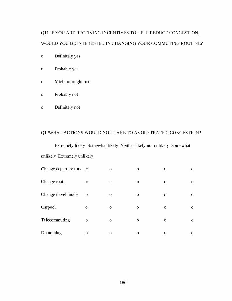
186
Q11 IF YOU ARE RECEIVING INCENTIVES TO HELP REDUCE CONGESTION,
WOULD YOU BE INTERESTED IN CHANGING YOUR COMMUTING ROUTINE?
o Definitely yes
o Probably yes
o Might or might not
o Probably not
o Definitely not
Q12WHAT ACTIONS WOULD YOU TAKE TO AVOID TRAFFIC CONGESTION?
Extremely likely Somewhat likely Neither likely nor unlikely Somewhat
unlikely Extremely unlikely
Change departure time o o o o o
Change route o o o o o
Change travel mode o o o o o
Carpool o o o o o
Telecommuting o o o o o
Do nothing o o o o o

187
Q13 WHICH OF THE FOLLOWING INCENTIVES WOULD MOTIVATE YOU TO
CHANGE YOUR TRAVEL HABITS TO REDUCE TRAFFIC CONGESTION?
Strongly agree Somewhat agree Neutral Somewhat disagree Strongly
disagree
Insurance discount o o o o o
Express lane access o o o o o
discounted parking o o o o o
Free/discounted tolls o o o o o
Discounted driver license renewal o o o o
o
Monetary reward o o o o o
Q14 DO YOU THINK DRIVING IS A RIGHT OR A PRIVILEGE?
o Driving is a right
o Driving is a privilege
o Not sure

188
Q15 DO YOU THINK IT IS GENERALLY A GOOD IDEA TO SUSPEND THE
DRIVING LICENSES OF CERTAIN DRIVERS?
o Strongly agree
o Somewhat agree
o Neutral
o Somewhat disagree
o Strongly disagree
Q16 HAVE YOU HEARD ABOUT CONNECTED VEHICLES TECHNOLOGY?
o Yes
o No
Q17 CONNECTED VEHICLE TECHNOLOGY ALLOWS THE RECORDING OF
REAL-TIME DATA ON VEHICLE MOVEMENT AND DRIVER PERFORMANCE.
DRIVERS COULD RECEIVE SCORES BASED ON THEIR DRIVING
PERFORMANCE. CONSIDER A TRAFFIC CONTROL STRATEGY THAT
PROVIDES DRIVERS ACCESS TO MAJOR HIGHWAYS BASED ON THEIR
DRIVING PERFORMANCE SCORES. FOR EXAMPLE, LOW-PERFORMING
DRIVERS COULD BE PROHIBITED FROM USING CERTAIN HIGHWAYS AT
CERTAIN TIME PERIODS. FOR MORE INFO, PLEASE WATCH THE
FOLLOWING VIDEO:

189
Q18 PLEASE RESPOND TO THE FOLLOWING STATEMENTS ABOUT THIS
TECHNOLOGY.
Strongly agree Somewhat agree Neither agree nor disagree Somewhat disagree
Strongly disagree
IT WILL MAKE MY TRAVEL SAFER o o o
o o
IT IS FAIR FOR ALL DRIVERS o o o o
o
IT WILL HELP ME IMPROVE MY DRIVING PERFORMANCE. o
o o o o
Q19 IF THIS TECHNOLOGY WERE DEPLOYED TODAY, WHAT WOULD YOUR
DRIVING SCORE BE?
o Excellent
o Very good
o Good
o Fair
o Poor

190
Q20 WOULD YOU SUPPORT THE DEPLOYMENT OF THIS TECHNOLOGY?
o Definitely yes
o Probably yes
o Probably not
o Definitely not
Q21 WHY WOULDN'T YOU SUPPORT THE DEPLOYMENT OF THIS
TECHNOLOGY?
▢ Privacy Concern
▢ Limit of route access
▢ It is impossible to be deployed
▢ Other
Q22 WHY WOULD YOU SUPPORT THE DEPLOYMENT OF THIS
TECHNOLOGY?
▢ Safety enhancement
▢ Faster commute
▢ Fairness (justice) among drivers

191
▢ Other
Q23 WHAT IS YOUR GENDER?
o Male
o Female
o Other
Q24 WHAT IS YOUR AGE GROUP?
o Under 16 years
o 16-20 years
o 21-24 years
o 25-29 years
o 30-34 years
o 35-39 years
o 40-49 years
o 50-60 years
o 60 years or older

192
Q25 WHAT IS YOUR RACE/ETHNICITY?
o White
o Hispanic or Latino
o Black or African American
o Asian
o American Indian or Alaska native
o Middle Eastern or North African
o Native Hawaiian or other Pacific Islander
o Other race or ethnicity
Q26 WHAT IS YOUR CURRENT MARITAL STATUS?
o Single, never married
o Married or in a domestic partnership
o Divorced
o Widowed
o Separated

193
Q27 HOW MANY CHILDREN DO YOU HAVE?
o Zero, I have no children
o One child
o Two children
o Three children
o More than three children
Q28 WHAT IS YOUR HIGHEST ACHIEVED LEVEL OF EDUCATION?
o Did not complete high school
o High school diploma
o Some college
o Bachelor's degree
o Master's degree
o Doctoral degree
Q29 WHAT IS YOUR CURRENT EMPLOYMENT STATUS?
o Employed full time (40 or more hours per week)
o Employed part time (up to 39 hours per week)
o Unemployed looking for work

194
o Unemployed not looking for work
o Retired
o Student
o Disabled
o Other
Q30 WHAT IS YOUR HOUSEHOLD INCOME?
o Less than $10,000
o $10,000 - $19,999
o $20,000 - $29,999
o $30,000 - $39,999
o $40,000 - $49,999
o $50,000 - $59,999
o $60,000 - $69,999
o $70,000 - $79,999
o $80,000 - $89,999
o $90,000 - $99,999
o $100,000 - $149,999
o More than $150,000

195
Q31 DO YOU LIVE AND/OR WORK IN AN URBAN AREA?
o Yes
o No
Q32 PLEASE ENTER YOUR 5-DIGIT ZIP CODE.

196
Appendix B
The Full Model
Coefficient Estimate Odds
Ratio 95% CI z value P-Value
Driving experience
(reference = less than 4 years)
4 - 10 years -0.71 0.49 (-1.23 , -
0.21)
-2.72 0.01
11 - 20 years -0.84 0.43 (-1.39 , -
0.32)
-3.11 0.00
More than 20 years -0.74 0.48 (-1.3 , -0.2) -2.63 0.01
Weekly commuting [days] 0.07 1.07 (0.01 , 0.14) 2.13 0.03
Number of tickets [last 5 years] 0.17 1.19 (-0.01 ,
0.36)
1.85 0.06
Points on DL (reference = no)
Yes 0.37 1.44 (-0.08 ,
0.83)
1.58 0.11
Congestion is a Commute Problem (reference= strongly disagree)
Somewhat disagree 0.44 1.55 (-0.12 , 1) 1.55 0.12
Neutral 0.74 2.09 (0.15 , 1.33) 2.46 0.01
Somewhat agree 0.63 1.89 (0.17 , 1.1) 2.69 0.01
Strongly agree 0.39 1.47 (-0.08 ,
0.85)
1.62 0.11
Willingness to change commuting routine (reference = extremely unlikely)
Somewhat unlikely 0.28 1.33 (-0.84 ,
1.44)
0.49 0.62
Neutral 0.12 1.13 (-0.9 , 1.19) 0.24 0.81
Somewhat likely 0.64 1.89 (-0.39 , 1.7) 1.21 0.23
Extremely likely 1.02 2.77 (-0.01 ,
2.09)
1.92 0.05
Change travel time
(reference = extremely unlikely)
Somewhat unlikely 0 1 (-0.7 , 0.69) 0 1
Neutral 0.88 2.41 (0.06 , 1.71) 2.11 0.03
Somewhat likely 0.38 1.46 (-0.27 ,
1.01)
1.16 0.25
Extremely likely 0.37 1.45 (-0.29 ,
1.02)
1.11 0.27
Change route
(reference = extremely unlikely)
Somewhat unlikely 0.6 1.83 (-0.35 ,
1.56)
1.24 0.21
Neutral -0.14 0.87 (-1.11 ,
0.83)
-0.28 0.78
Somewhat likely 0.16 1.18 (-0.69 ,
1.01)
0.38 0.7
Extremely likely -0.14 0.87 (-1 , 0.72) -0.31 0.76
Carpool
(reference = extremely unlikely)
Somewhat unlikely 0.21 1.24 (-0.15 ,
0.58)
1.14 0.25
Neutral 0.82 2.27 (0.38 , 1.27) 3.66 0.00
Somewhat likely 0.36 1.44 (-0.02 ,
0.74)
1.88 0.06
Extremely likely 0.19 1.21 (-0.31 , 0.7) 0.75 0.45
Free \ Discounted parking
(reference = extremely unlikely)
Somewhat unlikely 0.85 2.34 (0.04 , 1.68) 2.05 0.04
Neutral 0.96 2.62 (0.3 , 1.65) 2.82 0.00
Somewhat likely 0.86 2.36 (0.2 , 1.53) 2.54 0.01

197
Extremely likely 0.96 2.61 (0.29 , 1.65) 2.79 0.01
Free \ Discounted tolls
(reference = extremely unlikely)
Somewhat unlikely -1.02 0.36 (-1.91 , -
0.13)
-2.24 0.03
Neutral -0.73 0.48 (-1.5 , 0.01) -1.9 0.06
Somewhat likely -0.22 0.8 (-0.98 ,
0.51)
-0.59 0.56
Extremely likely -0.24 0.78 (-1.02 ,
0.51)
-0.62 0.53
DL suspension as punishment (reference=strongly disagree)
Somewhat disagree 0.64 1.9 (-0.82 ,
2.13)
0.86 0.39
Neutral 0.98 2.66 (-0.32 ,
2.32)
1.46 0.14
Somewhat agree 1.04 2.84 (-0.16 , 2.3) 1.67 0.09
Strongly agree 1.42 4.13 (0.22 , 2.67) 2.29 0.02
Connected vehicles familiarity
(reference = no)
Yes 0.3 1.35 (0 , 0.6) 1.97 0.05
Expected Score (reference=Excellent)
Poor -3.16 0.04 (-6.26 , -
0.83)
-2.53 0.01
Fair -1.58 0.21 (-2.36 , -
0.81)
-4.01 0.00
Good -1.18 0.31 (-1.56 , -0.8) -6.12 0.00
Very good -0.73 0.48 (-1.05 , -
0.42)
-4.58 0.00
Marital Status (reference=Divorced)
Married -0.09 0.91 (-0.69 ,
0.49)
-0.31 0.76
Separated 0.96 2.61 (-0.44 , 2.6) 1.27 0.2
Single -0.48 0.62 (-1.12 ,
0.14)
-1.5 0.13
Widowed 0.69 2 (-0.75 ,
2.37)
0.89 0.37
Number of children [years] 0.11 1.11 (-0.03 ,
0.25)
1.54 0.12
Household income (reference = < $50,000)
$50,000 - $99,999 0.25 1.28 (-0.04 ,
0.54)
1.68 0.09
$100,000 - $150,000 0.58 1.79 (0.16 , 1.01) 2.7 0.01
> $150,000 0.74 2.09 (0.28 , 1.21) 3.09 0.00
Outcome levels
Support | Do not Support
McFadden's R2 0.18
Nagelkerke R2 0.26
Log-likelihood -770.27
Akaike Information Criterion (AIC) 1644.55
Bayesian Information Criterion (BIC) 1725.43

198
Appendix C
The Univariate Model
Coefficient Estimate Odds
Ratio 95% CI z value P-Value
Driving experience
(reference = less than 4 years)
4 - 10 years -0.69 0.5 (-1.24, -0.16) -2.52 0.01
11 - 20 years -0.86 0.42 (-1.48 , -0.26) -2.75 0.01
More than 20 years -0.86 0.42 (-1.59 , -0.15) -2.34 0.02
Weekly commuting [days] 0.01 1.01 (-0.07 , 0.1) 0.34 0.73
Commute Distance
(reference = Less than 5 miles )
5 - 9 miles -0.21 0.81 (-0.63 , 0.2) -1.01 0.31
10 - 14 miles 0.11 1.12 (-0.31 , 0.53) 0.52 0.6
15 - 24 miles 0.26 1.3 (-0.17 , 0.7) 1.19 0.24
25 - 39 miles 0.13 1.14 (-0.39 , 0.66) 0.5 0.62
40 - 59 miles -0.18 0.83 (-0.86 , 0.51) -0.52 0.61
60 - 79 miles -0.17 0.84 (-1.24 , 0.91) -0.32 0.75
More than 80 miles 0.97 2.64 (-0.29 , 2.56) 1.37 0.17
Number of accidents [last 5 years] 0.03 1.03 (-0.16 , 0.23) 0.32 0.75
Number of tickets [last 5 years] 0.19 1.2 (-0.01 , 0.39) 1.83 0.07
Points on DL (reference = no)
Yes 0.41 1.51 (-0.05 , 0.9) 1.71 0.09
Congestion is a Commute Problem
(reference= strongly disagree)
Somewhat disagree 0.48 1.62 (-0.1 , 1.07) 1.62 0.1
Neutral 0.77 2.17 (0.15 , 1.41) 2.42 0.02
Somewhat agree 0.67 1.95 (0.16 , 1.17) 2.6 0.01
Strongly agree 0.36 1.43 (-0.16 , 0.87) 1.37 0.17
Willingness to change commuting routine
(reference = extremely unlikely)
Somewhat unlikely 0.33 1.4 (-0.85 , 1.56) 0.55 0.58
Neutral 0.27 1.31 (-0.84 , 1.42) 0.47 0.64
Somewhat likely 0.67 1.95 (-0.44 , 1.82) 1.17 0.24
Extremely likely 1.01 2.76 (-0.1 , 2.18) 1.76 0.08
Change travel time
(reference = extremely unlikely)
Somewhat unlikely 0.14 1.15 (-0.58 , 0.85) 0.38 0.71
Neutral 1.01 2.74 (0.17 , 1.85) 2.35 0.02
Somewhat likely 0.49 1.64 (-0.16 , 1.14) 1.49 0.14
Extremely likely 0.38 1.46 (-0.29 , 1.04) 1.11 0.27
Change mode
(reference = extremely unlikely)
Somewhat unlikely -0.04 0.96 (-0.48 , 0.4) -0.16 0.87

199
Neutral -0.11 0.89 (-0.59 , 0.37) -0.46 0.65
Somewhat likely -0.09 0.92 (-0.55 , 0.37) -0.37 0.71
Extremely likely -0.3 0.74 (-0.88 , 0.28) -1.01 0.31
Carpool
(reference = extremely unlikely)
Somewhat unlikely 0.35 1.41 (-0.07 , 0.76) 1.64 0.1
Neutral 0.89 2.43 (0.41 , 1.38) 3.6 0
Somewhat likely 0.42 1.51 (-0.02 , 0.85) 1.87 0.06
Extremely likely 0.3 1.35 (-0.28 , 0.88) 1.01 0.31
Telecommuting
(reference = extremely unlikely)
Somewhat unlikely -0.34 0.71 (-0.85 , 0.16) -1.33 0.18
Neutral -0.03 0.97 (-0.52 , 0.45) -0.14 0.89
Somewhat likely -0.07 0.93 (-0.54 , 0.39) -0.31 0.76
Extremely likely -0.36 0.7 (-0.8 , 0.08) -1.59 0.11
Do nothing
(reference = extremely unlikely)
Somewhat unlikely -0.11 0.9 (-0.56 , 0.35) -0.45 0.65
Neutral -0.22 0.8 (-0.61 , 0.17) -1.11 0.27
Somewhat likely -0.47 0.63 (-0.92 , -0.02) -2.04 0.04
Extremely likely 0 1 (-0.59 , 0.59) -0.01 0.99
Discounted Insurance
(reference = extremely unlikely)
Somewhat unlikely 0.04 1.04 (-1.28 , 1.36) 0.06 0.95
Neutral 0.22 1.25 (-1.01 , 1.44) 0.35 0.72
Somewhat likely 0.03 1.03 (-1.15 , 1.21) 0.06 0.95
Extremely likely 0.23 1.26 (-0.95 , 1.41) 0.39 0.7
Express Lane Access
(reference = extremely unlikely)
Somewhat unlikely 0.41 1.51 (-0.5 , 1.34) 0.88 0.38
Neutral 0.41 1.51 (-0.45 , 1.29) 0.93 0.35
Somewhat likely 0.53 1.71 (-0.31 , 1.38) 1.24 0.21
Extremely likely 0.69 1.99 (-0.18 , 1.56) 1.56 0.12
Free \ Discounted parking
(reference = extremely unlikely)
Somewhat unlikely 0.68 1.98 (-0.19 , 1.57) 1.53 0.13
Neutral 0.7 2.01 (-0.02 , 1.43) 1.89 0.06
Somewhat likely 0.69 1.98 (-0.03 , 1.41) 1.86 0.06
Extremely likely 0.71 2.02 (-0.03 , 1.45) 1.87 0.06
Free \ Discounted tolls
(reference = extremely unlikely)
Somewhat unlikely -0.98 0.38 (-1.96 , -0.02) -1.99 0.05
Neutral -0.87 0.42 (-1.71 , -0.05) -2.06 0.04
Somewhat likely -0.37 0.69 (-1.2 , 0.44) -0.87 0.38
Extremely likely -0.49 0.61 (-1.36 , 0.34) -1.14 0.25
Free \ Discounted DL renewal
(reference = extremely unlikely)
Somewhat unlikely 0.05 1.05 (-0.74 , 0.83) 0.12 0.91
Neutral 0.43 1.54 (-0.3 , 1.16) 1.17 0.24
Somewhat likely 0.5 1.66 (-0.21 , 1.21) 1.39 0.16
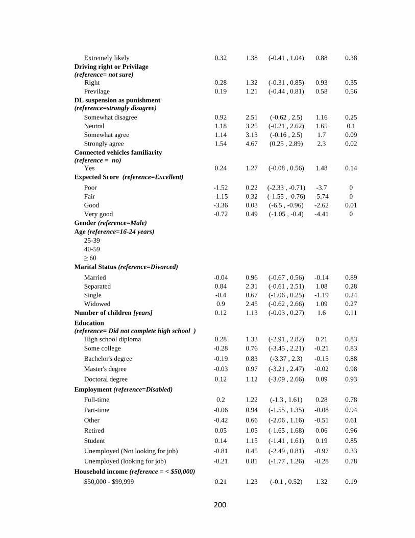
200
Extremely likely 0.32 1.38 (-0.41 , 1.04) 0.88 0.38
Driving right or Privilage
(reference= not sure)
Right 0.28 1.32 (-0.31 , 0.85) 0.93 0.35
Previlage 0.19 1.21 (-0.44 , 0.81) 0.58 0.56
DL suspension as punishment
(reference=strongly disagree)
Somewhat disagree 0.92 2.51 (-0.62 , 2.5) 1.16 0.25
Neutral 1.18 3.25 (-0.21 , 2.62) 1.65 0.1
Somewhat agree 1.14 3.13 (-0.16 , 2.5) 1.7 0.09
Strongly agree 1.54 4.67 (0.25 , 2.89) 2.3 0.02
Connected vehicles familiarity
(reference = no)
Yes 0.24 1.27 (-0.08 , 0.56) 1.48 0.14
Expected Score (reference=Excellent)
Poor -1.52 0.22 (-2.33 , -0.71) -3.7 0
Fair -1.15 0.32 (-1.55 , -0.76) -5.74 0
Good -3.36 0.03 (-6.5 , -0.96) -2.62 0.01
Very good -0.72 0.49 (-1.05 , -0.4) -4.41 0
Gender (reference=Male)
Age (reference=16-24 years)
25-39
40-59
≥ 60
Marital Status (reference=Divorced)
Married -0.04 0.96 (-0.67 , 0.56) -0.14 0.89
Separated 0.84 2.31 (-0.61 , 2.51) 1.08 0.28
Single -0.4 0.67 (-1.06 , 0.25) -1.19 0.24
Widowed 0.9 2.45 (-0.62 , 2.66) 1.09 0.27
Number of children [years] 0.12 1.13 (-0.03 , 0.27) 1.6 0.11
Education
(reference= Did not complete high school )
High school diploma
0.28 1.33 (-2.91 , 2.82) 0.21 0.83
Some college -0.28 0.76 (-3.45 , 2.21) -0.21 0.83
Bachelor's degree -0.19 0.83 (-3.37 , 2.3) -0.15 0.88
Master's degree -0.03 0.97 (-3.21 , 2.47) -0.02 0.98
Doctoral degree 0.12 1.12 (-3.09 , 2.66) 0.09 0.93
Employment (reference=Disabled)
Full-time 0.2 1.22 (-1.3 , 1.61) 0.28 0.78
Part-time -0.06 0.94 (-1.55 , 1.35) -0.08 0.94
Other -0.42 0.66 (-2.06 , 1.16) -0.51 0.61
Retired 0.05 1.05 (-1.65 , 1.68) 0.06 0.96
Student 0.14 1.15 (-1.41 , 1.61) 0.19 0.85
Unemployed (Not looking for job) -0.81 0.45 (-2.49 , 0.81) -0.97 0.33
Unemployed (looking for job) -0.21 0.81 (-1.77 , 1.26) -0.28 0.78
Household income (reference = < $50,000)
$50,000 - $99,999 0.21 1.23 (-0.1 , 0.52) 1.32 0.19

201
$100,000 - $150,000 0.51 1.67 (0.07 , 0.97) 2.23 0.03
> $150,000 0.58 1.78 (0.07 , 1.1) 2.18 0.03
Urbanity (reference=Yes) -0.08 0.93 (-0.37 , 0.21) -0.51 0.61
Outcome levels
Support | Do not Support

202
Appendix D
The Selection Model
Coefficient Estimate Odds
Ratio 95% CI z value P-Value
Commute Distance
(reference = Less than 5 miles )
5 - 9 miles -0.06 0.94 (-0.44 , 0.33) -0.29 0.771
10 - 14 miles 0.2 1.22 (-0.19 , 0.59) 0.99 0.32
15 - 24 miles 0.39 1.48 (-0.01 , 0.79) 1.93 0.054
25 - 39 miles 0.25 1.28 (-0.23 , 0.74) 1 0.319
40 - 59 miles -0.06 0.94 (-0.7 , 0.6) -0.18 0.858
60 - 79 miles -0.18 0.84 (-1.19 , 0.87) -0.34 0.737
More than 80 miles 1.1 3.01 (-0.13 , 2.67) 1.59 0.112
Points on DL (reference = no)
Yes 0.55 1.73 (0.11 , 1) 2.42 0.015
Willingness to change commuting routine
(reference = extremely unlikely)
Somewhat unlikely 0.62 1.86 (-0.53 , 1.81) 1.05 0.293
Neutral 0.51 1.66 (-0.56 , 1.61) 0.92 0.355
Somewhat likely 0.92 2.51 (-0.15 , 2.03) 1.67 0.094
Extremely likely 1.21 3.34 (0.13 , 2.32) 2.18 0.029
Change travel time
(reference = extremely unlikely)
Somewhat unlikely 0.14 1.15 (-0.56 , 0.83) 0.4 0.691
Neutral 1.02 2.78 (0.21 , 1.84) 2.47 0.014
Somewhat likely 0.48 1.62 (-0.16 , 1.11) 1.5 0.134
Extremely likely 0.32 1.37 (-0.34 , 0.96) 0.96 0.336
Change mode
(reference = extremely unlikely)
Somewhat unlikely -0.05 0.95 (-0.47 , 0.37) -0.23 0.822
Neutral -0.12 0.88 (-0.59 , 0.34) -0.52 0.605
Somewhat likely -0.1 0.9 (-0.55 , 0.34) -0.45 0.653
Extremely likely -0.33 0.72 (-0.89 , 0.24) -1.14 0.256
Carpool
(reference = extremely unlikely)
Somewhat unlikely 0.26 1.3 (-0.13 , 0.66) 1.3 0.194
Neutral 0.89 2.43 (0.42 , 1.36) 3.72 0
Somewhat likely 0.39 1.47 (-0.03 , 0.8) 1.82 0.069
Extremely likely 0.18 1.2 (-0.37 , 0.74) 0.64 0.524
Do nothing
(reference = extremely unlikely)
Somewhat unlikely -0.04 0.96 (-0.48 , 0.41) -0.16 0.873
Neutral -0.19 0.83 (-0.57 , 0.18) -0.99 0.322
Somewhat likely -0.42 0.66 (-0.85 , 0.01) -1.9 0.057
Extremely likely -0.01 0.99 (-0.57 , 0.56) -0.04 0.967
Discounted Insurance
(reference = extremely unlikely)
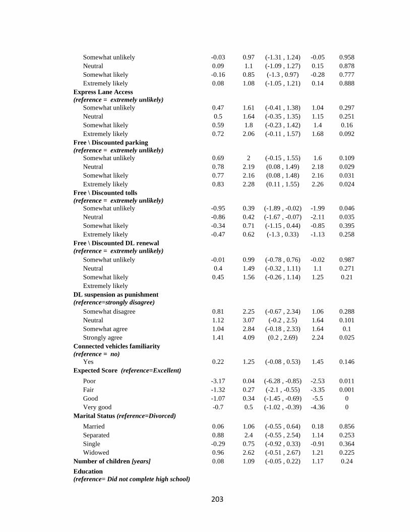
203
Somewhat unlikely -0.03 0.97 (-1.31 , 1.24) -0.05 0.958
Neutral 0.09 1.1 (-1.09 , 1.27) 0.15 0.878
Somewhat likely -0.16 0.85 (-1.3 , 0.97) -0.28 0.777
Extremely likely 0.08 1.08 (-1.05 , 1.21) 0.14 0.888
Express Lane Access
(reference = extremely unlikely)
Somewhat unlikely 0.47 1.61 (-0.41 , 1.38) 1.04 0.297
Neutral 0.5 1.64 (-0.35 , 1.35) 1.15 0.251
Somewhat likely 0.59 1.8 (-0.23 , 1.42) 1.4 0.16
Extremely likely 0.72 2.06 (-0.11 , 1.57) 1.68 0.092
Free \ Discounted parking
(reference = extremely unlikely)
Somewhat unlikely 0.69 2 (-0.15 , 1.55) 1.6 0.109
Neutral 0.78 2.19 (0.08 , 1.49) 2.18 0.029
Somewhat likely 0.77 2.16 (0.08 , 1.48) 2.16 0.031
Extremely likely 0.83 2.28 (0.11 , 1.55) 2.26 0.024
Free \ Discounted tolls
(reference = extremely unlikely)
Somewhat unlikely -0.95 0.39 (-1.89 , -0.02) -1.99 0.046
Neutral -0.86 0.42 (-1.67 , -0.07) -2.11 0.035
Somewhat likely -0.34 0.71 (-1.15 , 0.44) -0.85 0.395
Extremely likely -0.47 0.62 (-1.3 , 0.33) -1.13 0.258
Free \ Discounted DL renewal
(reference = extremely unlikely)
Somewhat unlikely -0.01 0.99 (-0.78 , 0.76) -0.02 0.987
Neutral 0.4 1.49 (-0.32 , 1.11) 1.1 0.271
Somewhat likely 0.45 1.56 (-0.26 , 1.14) 1.25 0.21
Extremely likely
DL suspension as punishment
(reference=strongly disagree)
Somewhat disagree 0.81 2.25 (-0.67 , 2.34) 1.06 0.288
Neutral 1.12 3.07 (-0.2 , 2.5) 1.64 0.101
Somewhat agree 1.04 2.84 (-0.18 , 2.33) 1.64 0.1
Strongly agree 1.41 4.09 (0.2 , 2.69) 2.24 0.025
Connected vehicles familiarity
(reference = no)
Yes 0.22 1.25 (-0.08 , 0.53) 1.45 0.146
Expected Score (reference=Excellent)
Poor -3.17 0.04 (-6.28 , -0.85) -2.53 0.011
Fair -1.32 0.27 (-2.1 , -0.55) -3.35 0.001
Good -1.07 0.34 (-1.45 , -0.69) -5.5 0
Very good -0.7 0.5 (-1.02 , -0.39) -4.36 0
Marital Status (reference=Divorced)
Married 0.06 1.06 (-0.55 , 0.64) 0.18 0.856
Separated 0.88 2.4 (-0.55 , 2.54) 1.14 0.253
Single -0.29 0.75 (-0.92 , 0.33) -0.91 0.364
Widowed 0.96 2.62 (-0.51 , 2.67) 1.21 0.225
Number of children [years] 0.08 1.09 (-0.05 , 0.22) 1.17 0.24
Education
(reference= Did not complete high school)
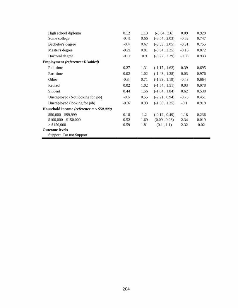
204
High school diploma
0.12 1.13 (-3.04 , 2.6) 0.09 0.928
Some college -0.41 0.66 (-3.54 , 2.03) -0.32 0.747
Bachelor's degree -0.4 0.67 (-3.53 , 2.05) -0.31 0.755
Master's degree -0.21 0.81 (-3.34 , 2.25) -0.16 0.872
Doctoral degree -0.11 0.9 (-3.27 , 2.39) -0.08 0.933
Employment (reference=Disabled)
Full-time 0.27 1.31 (-1.17 , 1.62) 0.39 0.695
Part-time 0.02 1.02 (-1.43 , 1.38) 0.03 0.976
Other -0.34 0.71 (-1.93 , 1.19) -0.43 0.664
Retired 0.02 1.02 (-1.54 , 1.51) 0.03 0.978
Student 0.44 1.56 (-1.04 , 1.84) 0.62 0.538
Unemployed (Not looking for job) -0.6 0.55 (-2.21 , 0.94) -0.75 0.451
Unemployed (looking for job) -0.07 0.93 (-1.58 , 1.35) -0.1 0.918
Household income (reference = < $50,000)
$50,000 - $99,999 0.18 1.2 (-0.12 , 0.49) 1.18 0.236
$100,000 - $150,000 0.52 1.69 (0.09 , 0.96) 2.34 0.019
> $150,000 0.59 1.81 (0.1 , 1.1) 2.32 0.02
Outcome levels
Support | Do not Support
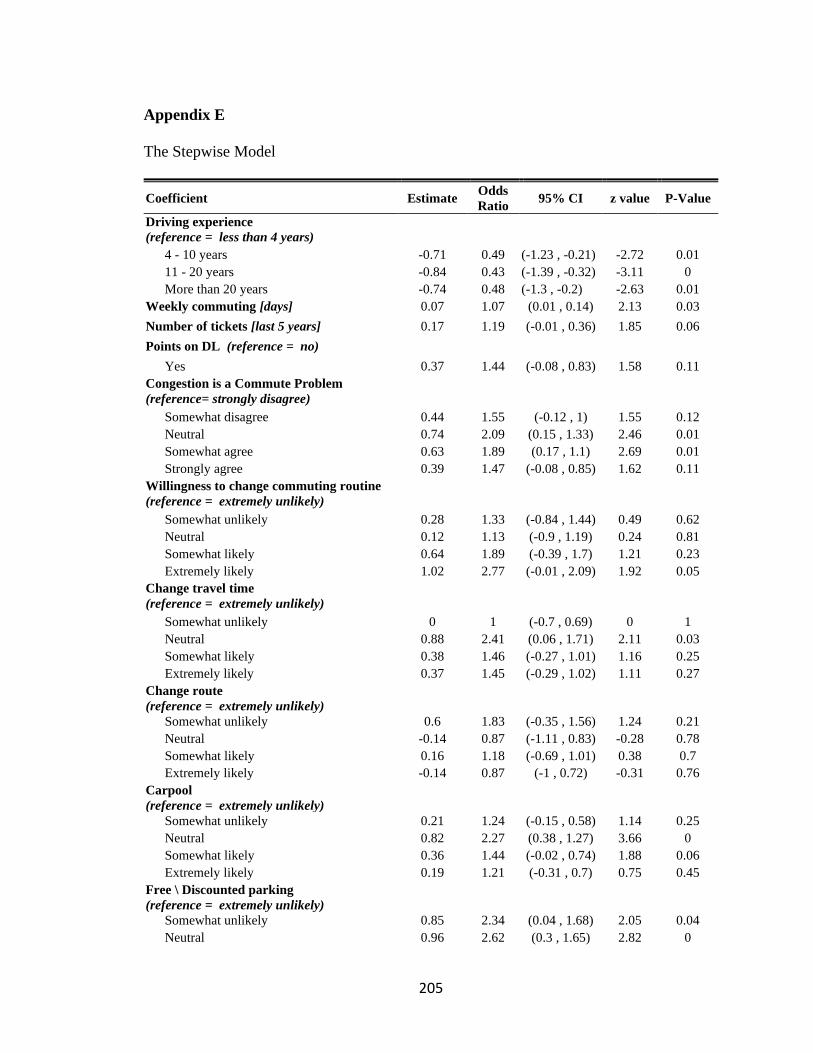
205
Appendix E
The Stepwise Model
Coefficient Estimate Odds
Ratio 95% CI z value P-Value
Driving experience
(reference = less than 4 years)
4 - 10 years -0.71 0.49 (-1.23 , -0.21) -2.72 0.01
11 - 20 years -0.84 0.43 (-1.39 , -0.32) -3.11 0
More than 20 years -0.74 0.48 (-1.3 , -0.2) -2.63 0.01
Weekly commuting [days] 0.07 1.07 (0.01 , 0.14) 2.13 0.03
Number of tickets [last 5 years] 0.17 1.19 (-0.01 , 0.36) 1.85 0.06
Points on DL (reference = no)
Yes 0.37 1.44 (-0.08 , 0.83) 1.58 0.11
Congestion is a Commute Problem
(reference= strongly disagree)
Somewhat disagree 0.44 1.55 (-0.12 , 1) 1.55 0.12
Neutral 0.74 2.09 (0.15 , 1.33) 2.46 0.01
Somewhat agree 0.63 1.89 (0.17 , 1.1) 2.69 0.01
Strongly agree 0.39 1.47 (-0.08 , 0.85) 1.62 0.11
Willingness to change commuting routine
(reference = extremely unlikely)
Somewhat unlikely 0.28 1.33 (-0.84 , 1.44) 0.49 0.62
Neutral 0.12 1.13 (-0.9 , 1.19) 0.24 0.81
Somewhat likely 0.64 1.89 (-0.39 , 1.7) 1.21 0.23
Extremely likely 1.02 2.77 (-0.01 , 2.09) 1.92 0.05
Change travel time
(reference = extremely unlikely)
Somewhat unlikely 0 1 (-0.7 , 0.69) 0 1
Neutral 0.88 2.41 (0.06 , 1.71) 2.11 0.03
Somewhat likely 0.38 1.46 (-0.27 , 1.01) 1.16 0.25
Extremely likely 0.37 1.45 (-0.29 , 1.02) 1.11 0.27
Change route
(reference = extremely unlikely)
Somewhat unlikely 0.6 1.83 (-0.35 , 1.56) 1.24 0.21
Neutral -0.14 0.87 (-1.11 , 0.83) -0.28 0.78
Somewhat likely 0.16 1.18 (-0.69 , 1.01) 0.38 0.7
Extremely likely -0.14 0.87 (-1 , 0.72) -0.31 0.76
Carpool
(reference = extremely unlikely)
Somewhat unlikely 0.21 1.24 (-0.15 , 0.58) 1.14 0.25
Neutral 0.82 2.27 (0.38 , 1.27) 3.66 0
Somewhat likely 0.36 1.44 (-0.02 , 0.74) 1.88 0.06
Extremely likely 0.19 1.21 (-0.31 , 0.7) 0.75 0.45
Free \ Discounted parking
(reference = extremely unlikely)
Somewhat unlikely 0.85 2.34 (0.04 , 1.68) 2.05 0.04
Neutral 0.96 2.62 (0.3 , 1.65) 2.82 0

206
Somewhat likely 0.86 2.36 (0.2 , 1.53) 2.54 0.01
Extremely likely 0.96 2.61 (0.29 , 1.65) 2.79 0.01
Free \ Discounted tolls
(reference = extremely unlikely)
Somewhat unlikely -1.02 0.36 (-1.91 , -0.13) -2.24 0.03
Neutral -0.73 0.48 (-1.5 , 0.01) -1.9 0.06
Somewhat likely -0.22 0.8 (-0.98 , 0.51) -0.59 0.56
Extremely likely -0.24 0.78 (-1.02 , 0.51) -0.62 0.53
Free \ Discounted DL renewal
(reference = extremely unlikely)
Somewhat unlikely 0.64 1.9 (-0.82 , 2.13) 0.86 0.39
Neutral 0.98 2.66 (-0.32 , 2.32) 1.46 0.14
Somewhat likely 1.04 2.84 (-0.16 , 2.3) 1.67 0.09
Extremely likely 1.42 4.13 (0.22 , 2.67) 2.29 0.02
DL suspension as punishment
(reference=strongly disagree)
Somewhat disagree 0.3 1.35 (0 , 0.6) 1.97 0.05
Neutral
Somewhat agree -3.16 0.04 (-6.26 , -0.83) -2.53 0.01
Strongly agree -1.58 0.21 (-2.36 , -0.81) -4.01 0
Connected vehicles familiarity
(reference = no)
-1.18 0.31 (-1.56 , -0.8) -6.12 0
Yes -0.73 0.48 (-1.05 , -0.42) -4.58 0
Marital Status (reference=Divorced)
Married -0.09 0.91 (-0.69 , 0.49) -0.31 0.76
Separated 0.96 2.61 (-0.44 , 2.6) 1.27 0.2
Single -0.48 0.62 (-1.12 , 0.14) -1.5 0.13
Widowed 0.69 2 (-0.75 , 2.37) 0.89 0.37
Number of children [years] 0.11 1.11 (-0.03 , 0.25) 1.54 0.12
Household income (reference = < $50,000)
$50,000 - $99,999 0.25 1.28 (-0.04 , 0.54) 1.68 0.09
$100,000 - $150,000 0.58 1.79 (0.16 , 1.01) 2.7 0.01
> $150,000 0.74 2.09 (0.28 , 1.21) 3.09 0
Outcome levels
Support | Do not Support