an initial overview of iwan modeling for mechanical...

SANDIA REPORTSAND2001-0811Unlimited ReleasePrinted March 2001

An Initial Overview of Iwan Modeling forMechanical Joints

Daniel J. Segalman

Prepared bySandia National LaboratoriesAlbuquerque, New Mexico 87185 and Livermore, California 94550

Sandia is a multiprogram laboratory operated by Sandia Corporation,a Lockheed Martin Company, for the United States Department ofEnergy under Contract DE-AC04-94AL85000.

Approved for public release; further dissemination unlimited.

Issued by Sandia National Laboratories, operated for the United States Departmentof Energy by Sandia Corporation.

NOTICE: This report was prepared as an account of work sponsored by an agencyof the United States Government. Neither the United States Government, nor anyagency thereof, nor any of their employees, nor any of their contractors,subcontractors, or their employees, make any warranty, express or implied, orassume any legal liability or responsibility for the accuracy, completeness, orusefulness of any information, apparatus, product, or process disclosed, or representthat its use would not infringe privately owned rights. Reference herein to anyspecific commercial product, process, or service by trade name, trademark,manufacturer, or otherwise, does not necessarily constitute or imply its endorsement,recommendation, or favoring by the United States Government, any agency thereof,or any of their contractors or subcontractors. The views and opinions expressedherein do not necessarily state or reflect those of the United States Government, anyagency thereof, or any of their contractors.

Printed in the United States of America. This report has been reproduced directlyfrom the best available copy.

Available to DOE and DOE contractors fromU.S. Department of EnergyOffice of Scientific and Technical InformationP.O. Box 62Oak Ridge, TN 37831

Telephone: (865)576-8401Facsimile: (865)576-5728E-Mail: [email protected] ordering: http://www.doe.gov/bridge

Available to the public fromU.S. Department of CommerceNational Technical Information Service5285 Port Royal RdSpringfield, VA 22161

Telephone: (800)553-6847Facsimile: (703)605-6900E-Mail: [email protected] order: http://www.ntis.gov/ordering.htm

mailto:[email protected]

mailto:[email protected]

SAND2001-0811Unlimited Release March 2001

An Initial Overview of Iwan Modeling

for Mechanical Joints

Daniel J. SegalmanStructural Mechanics and Vibration Control Division

Sandia National LaboratoriesP.O. Box 5800

Albuquerque, NM 87185-0847

ABSTRACT

The structural dynamics modeling of engineering structures must accommodate the energy dissipation due to microslip in mechanical joints. Given the nature of current hardware and software environments, this will require the development of constitutive models for joints that both adequately reproduce the important physics and lend themselves to efficient computational processes. The exploration of the properties of mechanical joints - either through fine resolution finite element modelling or through experiment - is itself an area of research, but some qualitative behavior appears to be established. The work presented here is the presentation of a formulation of idealized elements due to Iwan, that appears capable of reproducing the important joint properties as they are now understood. Further, methods for selecting parameters for that model by joining the results from experiments in regimes of small and large load are developed. The significance of this work is that a reduced order model is presented that is capable of reproducing the important qualitative properties of mechanical joints using only a small number of parameters.

Acknowledgments

The observations presented in this report grew out of an evolving understanding that could not have taken place without enthusiastic and helpful discussions with fellow Sandians: Jeffrey Dohner, Danny Gregory, David Smallwood, and Todd Simmermacher. Discussion with Danny Gregory and David Smallwood were made especially valuable by their insight into interpretation of experimental results, both their own and those found in the literature. Finally, credit has to be given to the managers, David Martinez, Jamie Moya, and Wendell Kawahara, who have given continuous funding and moral support for this research effort.

Contents

Introduction 1

Micro-slip at Joints 2

Dissipation Mechanisms 11

Asymptotic Form 14

Model Reduction 18

Discrete Models 19

Energy Dissipation Due to Harmonic Loading 23

Limit of Small Force 24

Large Force Response 33

Model Parameters 34

Conclusions 37

References 38

Appendix A: The Residual Slip Experiment 41

Appendix B: Significance of the Dissipation Parameter 45

Appendix C: Example Finite Element Calculation 49

Figures

Figure 1. Slip in a joint occurs in a subset of the contact patch. 10

Figure 2. The Goodman hypothesis is illustrated in a one-dimensional problem. 12

Figure 3. The geometry of Hertzian contact. 15

Figure 4. Iwan parallel-series systems (a) and series-parallel systems (b). 20

Figure 5. An augmented Iwan model is used to represent a mechanical joint. 22

Figure 6. Test case using non-sinusoidal applied force 29

Figure 7. Resulting time derivative of displacement u(t) 30

Figure 8. Instantaneous net force from all sliding Iwan elements. 31

Figure 9. Resulting dissipation rates are identical for both cases. 32

Mathematical Symbols

radius of contact region in Mindlin solution for Hertzian contact indicated in Figure 3. First used in Equation 15.

total contact area of an interface. First used in Equation 1.

the portion of the contact area undergoing slip. First used in Equation 1.

cross-sectional area in strip-slip calculation indicated in Figure 2. First used in Equation 3.

Euler beta function. First used in Equation 14.

radius of non-slip region in Mindlin solution for Hertzian contact indicated in Figure 3. First used in Equation 15.

proportionality coefficient between normal traction and distance along slip

length. First used in Equation 11.

proportionality coefficient between slip length and applied force. First used in

Equation 10.

proportionality coefficient between lateral displacement and distance from tip

of slip length. First used in Equation 12.

Young’s modulus in strip-slip calculation indicated in Figure 2. First used in Equation 3.

energy dissipation per cycle. First used in Equation 8.

amplitude of oscillatory force in harmonic loading. First used in Equation 5.

maximum applied force magnitude anticipated over a given history. First used

in Equation 36.

shear modulus. First used in Equation 17.

stiffness of the soft spring in the augmented Iwan model shown in Figure 5. First

used in Equation 52.

total stiffness of the contact patch. First used in Equation 38.

the spring stiffness of the Iwan elements in the networks indicated in Figures 4a and 5. First used in this sense in Equation 28.

a

AC

AS

A

B( )

c

Cp

CS

Cu

E

D

F0

FM

G

K1

KT

k

instantaneous length of the slip regime in strip-slip calculation indicated in Figure 2. First used in Equation 5.

normal traction in strip-slip calculation indicated in Figure 2. First used in Equation 3.

total normal force. First used in Equation 15.

average normal traction in contact region in Mindlin solution for Hertzian

contact indicated in Figure 3. First used in Equation 16.

local normal traction at location . First used in Equation 9.

multiplicative coefficient in power-law expression for population density of Iwan models. First used in Equation 45.

total displacement of augmented Iwan network in Figure 5. First used in Equation 52.

displacement in strip-slip calculation indicated in Figure 2. First used in Equation 3.

displacement of the parallel Iwan elements indicated in Figures 4a and 5. First used in this sense in Equation 27.

distance from free surface of slip domain. Indicated in Figures 2 and 3.

displacement of slider element whose “break free” force is at time , indicated in Figures 4a and 5. First used in this sense in Equation 28.

dimensionless distance from the tip of the slip region in Mindlin solution for Hertzian contact indicated in Figure 3. First used in Equation 17.

dimensionless distance from the tip of the slip region in Mindlin solution for Hertzian contact indicated in Figure 3. First used in Equation 17.

exponent in proportionality between normal traction and distance along slip length. First used in Equation 11.

exponent in proportionality between slip length and applied force. First used in Equation 21.

exponent in proportionality between lateral displacement and distance from tip of slip length. First used in this sense in Equation 21.

exponent in proportionality between coefficient of friction and normal traction. First used in this sense in Equation 23.

L t( )

N

P

p0

p x( ) x

R

U t( )

u x t,( )

u t( )

x

x φ t,( ) φ t

z

z

α

β

γ

γ

exponent in proportionality between dissipation per cycle and applied force. First used in this sense in Equation 26.

multiplicative coefficient in power-law expression for dissipation resulting from power-law form of population density. First used in this sense in Equation 47.

the nth moment of the population density:

friction coefficient in strip-slip calculation indicated in Figure 2. First used in Equation 3.

the population density of Iwan elements whose “break free” force is . First used in this sense in Equation 28.

the value of “break free” force is selected from the region of overlap between low-force experiments where dissipation data is available and high force experiments where softening data is available.

exponent in power-law expression for population density of Iwan models. First used in Equation 45.

γ

ϑ

Λn θ( ) Λn θ( ) ρ φ( )φn φd

0

θ

∫=

ν

ρ φ( ) φ

φ φ

χ

Introduction

Constitutive modeling of mechanical joints appears to be gaining increased interest, as

indicated by the occurrence of several recent and forthcoming workshops and symposia.

That interest would appear to be motivated by the availability of new computational and

experimental tools and the perception that the design process for many dynamic systems

can be made much more economic by increased reliance on predictive simulation.

This work is driven by the definition that predictive modeling is that which provides

reliable quantitative information without first requiring the construction of a prototype.

Even this is a matter of degree: Analysis of a design radically different from anything built

before requires much more prowess on the part of the analyst to be predictive than does

analysis of a design which is a small departure from that which has been built and tested.

Constitutive modeling of mechanical joints is an important part of predictive dynamic

modeling of jointed structures because the joints are often the dominant source of energy

dissipation and vibration damping in those structures. For very expensive components or

components that are safety critical, predictive dynamic modeling is necessary. Jointed

structures that fit those criteria include turbine blades and nuclear weapons. The intent of

this monograph is to present some ideas that should be directly applicable to the predictive

dynamic modeling of such structures for an important regime of excitation - that for which

the excitation is sufficient to cause significant energy dissipation but for which the

displacements are so minute as to make direct measurement of kinematics impossible.

This is the micro-slip regime.

Micro-slip at Joints

The notion of micro-slip at a joint is

illustrated in Figure 1, where a bolt is

used to connect two thick components.

There is presumed to be a large

prestress in the bolt and a

corresponding region of large normal

stress between the components in the

vicinity of the bolt. A tangential load will cause slip in some region where the normal

tractions are not so large as to prevent it. Because slip occurs in a small region, the

magnitude of slip displacement is small, and there is no gross slip at the joint; this

mechanism is usually described as “micro-slip”. The major complication in the analytic

prediction of energy dissipation associated with micro-slip is the calculation of the slip

region.

The term “micro-slip” is sometimes used interchangeably with the term “partial slip”, and

this practice has lead to occasional serious misunderstanding. The author would like to

suggest that the term “partial slip” should be used for all cases where the slip region is less

than the full contact patch - this is any case involving slip short of complete sliding:

(1)

where is the area of slip and is the total contact area. The term “micro-slip” should

be reserved for cases for which the contact area over which slip occurs is much less than

the total contact area:

No-Slip

Region of

Sliding

Region

Frictional

“Slip”Figure 1. Slip in a joint occurs in a subset of the contact patch.

0 A< S AC<

AS AC

(2)

throughout the history of interest.

This importance of this distinction becomes evident when one contrasts convergence

studies of micro-slip analysis - which most likely will involve extraordinarily small

meshing - with convergence studies of large partial slip.

Dissipation MechanismsEnergy dissipation at bolted joints has been associated with several distinct mechanisms.

This subject was investigated intently by Eric Ungar[1,2] in the early 1960’s with an

ingenious set of calculations and experiments, studying many factors including joint

spacing, joint tightness, flange material and surface finish. Ungar considered oscillatory

loads and examined several postulated dissipation mechanisms, computing for each the

manner in which energy dissipation would be expected to increase with load. Ungar found

that, though there were unknown parameters in those expressions, each mechanism

manifested a dissipation rate increasing as a distinct power of the amplitude of the applied

load. Ungar then examined experimental data, evaluating the slope of dissipation versus

applied force amplitude when plotted in a log-log manner. In those experiments, which

concerned thin plates bolted together, Ungar concluded that the dominant mechanism of

energy dissipation was air pumping between the plates in the vicinities of the bolted

connections. Part of the basis for that conclusion was the observation that the slope of the

log-log plot of dissipation versus force was on the order of 2.0, corresponding to viscous

dissipation. When the joints were loosened so that there could be significant macro-slip,

the slope of the log-log plots increased to 2.5. Ungar’s experiments focussed on

geometries then most relevant to aircraft bodies. These involved thin plates with

0 A< S AC«

significant bending compliance, and were qualitatively different from the problems of

interest here; but Ungar’s methods still have value to us. Ungar focused attention on use of

the dependence of energy dissipation on amplitude of applied force as a tool to identify

dissipation mechanisms.

Where thick sections are bolted together, energy dissipation is generally associated with

micro-slip near the bolt and corresponding frictional losses. Goodman[8] observed that

several particular calculations of systems that involve slip and Coulomb friction

manifested energy dissipation growing as force amplitude to the third power. He

generalized that result to that subset of systems of elastic components sharing a frictional

interface, held together by a normal force, and perturbed by an oscillatory tangential load

for whichthe region of slip increases linearly with the amplitude of tangential force. The

derivation will not be developed here, but the core elements are demonstrated by

consideration of a semi-infinite rod held in a semi-infinite vise, as shown in Figure 2. The

rod is assumed to be elastic and the normal traction applied by the vise is assumed to be

uniform. When the applied force is maximum in the cycle, the region of slip is also at its

F0sin(ωt)

L(F0)

Figure 2. The Goodman hypothesis is illustrated in a one-dimensional problem.

maximum, extending from the origin to location , where is the amplitude of the

oscillatory force. Within the region of slip, the equilibrium equation is:

(3)

where is Young’s modulus, is cross sectional area of the rod, is the

displacement of the rod at location , is the normal traction, and is the coefficient of

Coulomb friction. (No distinction is made between static and dynamic friction). Note,

Poisson contraction is ignored here. Beyond the slip region,

. (4)

Because Equation 3 is second order and is as yet un-specified, all three of the following

boundary conditions are required:

; ; and (5)

The solution at maximum extension is

(6)

for . (7)

The energy dissipation over a full cycle is

. (8)

This example problem illustrates each of the components that Goodman asserts in his

general derivation for problems of oscillatory tangential loads applied to linear objects

sharing a frictional interface:

L F0( ) F0

EAx

2

2

∂∂ u

2Nν=

E A u x( )

x N ν

u x( ) 0≡

L

u L( ) 0= u’ L( ) 0= u’ 0( ) F– 0 EA⁄=

L12---

F0

Nν-------=

u x( ) NνEA------- L x–( )2

= 0 x L< <

D 4 2Nν( )u x( ) xd

0

L F0( )

∫ 23---

F03

EA 2Nν( )2--------------------------= =

1. the region of slip increases linearly with amplitude of applied load;

2. and the energy dissipation is proportional to the third power of the amplitude of applied force.

Asymptotic FormNote that in general, in oscillatory loading, the energy dissipation over each cycle is

(9)

where is the normal traction at location . For the example elasticity problem

considered above the slip length, normal traction, and the slip displacement have the

forms:

, (10)

, and (11)

. (12)

The energy dissipation is

(13)

(14)

where is the Euler beta function[3].

For the example considered above, , , and (satisfying the

Goodman hypothesis).

Goodman used the problem of contacting spheres subject to small lateral slip to illustrate

his observation about frictional dissipation. That problem, having normal force P and

D 4 νp x( )u x( ) xd

0

L F0( )

∫=

p x( ) x

L CSF0=

p x( ) Cpxα

=

u x( ) Cu L x–( )β=

D 4νCpCu xα

L x–( )β xd

0

L F0( )

∫=

4νCpCuCSα β 1+ +

B α 1 β 1+,+( )[ ]F0α β 1+ +

=

B( )

α 0= β 2= α β 1+ + 3=

lateral force F0, contact radius a, and no-slip radius c, is illustrated in the following figure.

The coordinate from the free surface toward the slip/no-slip interface is indicated by x. For

that problem, whose solution was worked out by Mindlin[4] and Cattaneo[5]

independently, the closed form solutions are provided by Johnson[6]:

, (15)

, (16)

and ,(17)

where , is Poisson’s ratio, is shear modulus, and . Note

that is the distance from the slip/no-slip interface to location . For the case of micro-

slip (expressed in this case by ), the above expressions can be written:

P

P

c

a

x

Figure 3. The geometry of Hertzian contact.

F0

F0

ca--- 1

F0

νP-------–

1 2⁄

=

p x( ) p0 1 1xa---+

2–

1 2⁄=

u x( ) 3νP16Ga-------------- 2 µ–( ) 1

2π--- 1

1 z+-----------asin–

1 21

1 z+----------- 2

– 2

π---

11 z+----------- 1

11 z+----------- 2

–

12---

+

=

p0 2Pπa------= µ G z

a c–( ) x–c

-------------------------=

cz x

a c–( ) c 1«⁄

, (18)

, (19)

and

. (20)

So here we see that the slip length is again proportional to the lateral load. We also identify

, , and observe that again.

Experimental results are generally disappointing for the analyst. In general, the

experimentalists do find that micro-slip yields a power-law relationship between lateral

load and energy dissipation, but they tend to find exponents closer to 2.5 rather than 3.0.

(Johnson(1961) and Ungar(1967)). Various explanations have been offered, most of which

come down to the assertion that Coulomb friction may not be an adequate model for the

dissipation taking place in the slip region. Johnson (ibid) asserts that the true dissipation

involves metal plasticity not accounted for by Amonton’s law. Gaul (1997) suggests that

the calculation of dissipation in the region of small normal stresses requires direct

accounting for asperity to asperity interaction, resulting in a different kind of friction law.

Recent experiments at Sandia National Laboratories by Smallwood, Gregory and

Coleman (2000) suggest values between 2.6 and 2.9 for the power-law relationship

between lateral load and energy dissipation. The construction of low-order models both

for the case of slope 3.0 and for cases for slope less than 3.0 is discussed below.

There are various ways that the conditions of Goodman’s analysis can be weakened and

still yield a power-law relation between tangential load and dissipation. In particular,

a c–aF0

2νP----------=

p x( ) p0 x a⁄( )1 2⁄=

u x( ) νPGa------- 2 µ–( ) 2

π-------z

3 2⁄=

α 1 2⁄= β 3 2⁄= α β 1+ + 3=

α

and need not sum to . Further, the relationship between tangential load and the length

of the slip region need not be linear. If the slip region is related to the maximum amplitude

of the tangential load in the following manner,

(21)

then analysis such as that which leads to Equation 14 yields

. (22)

A more interesting case is that in which the pressure and displacement results of the

classical solutions are preserved, but that the friction law is altered. This exploration is

consistent with the observation that micro-slip occurs in regions of very low normal

traction where Amonton’s law might not be valid. It is anticipated that some other physics

apply in the regime of low normal tractions and that as the normal traction is increased

that behavior gradually converges into Coulomb friction. One model of friction in the

region of low pressure involves pressure dependent friction coefficients (Rabinowicz,

1995), the simplest of which is

. (23)

The dissipation becomes

. (24)

If we accept the portion of the Goodman assertion that and that ,

then we find that

. (25)

β 2

L F0γ∝

D F0γ α β 1+ +( )∝

ν p( ) ν0pp0----- γ

=

D 4ν0Cu Cp1 γ+

p0γ⁄( )Lα β 1+ +

Lαγ

=

α β+ 2= L CLF=

D F03 αγ+∝

If the friction law used above is a good approximation for reality when is a slightly

negative number, this result becomes valuable on two counts:

• the model supports the deviation of experiment from Goodman’s hypothesis in the

correct direction;

• the model predicts a different power-law relationship for each type of contact (spheri-

cal contact, plate contact, strip contact). We now have some predictions to test against

experiment.

Whether Equations 11, 12, 23 can adequately describe the physics of joint slip is still a

matter of research. Ideally, a continuum level (finite element) model, properly

accommodating all of the relevant physics could explain power-law dissipation relations

and determine the relevant parameters.

The above discussion has explored methods by which either analytic elasticity or finite

element tools can be employed to derive an expression for dissipation of the form

(26)

and methods for predicting appropriate values of the parameters and . We shall see

below that these quantities are enough to determine parameters for limited constitutive

models for jointed structures.

Model Reduction

Whatever physics hold in joint interfaces, detailed solution of those equations as part of

a finite element model for the whole structure would introduce hundreds of new

unknowns for each joint, each unknown associated with a nonlinear equation. Further,

γ

D AF0γ

=

A γ

capturing those degrees of freedom would be associated with extremely small elements,

dramatically reducing the characteristic time step of the problem. These limitations make

such an approach impractical. Instead, one strives to devise low order models - on the

order of tens of degrees of freedom - to represent the region of the structure surrounding

the joint. The small number of associated nonlinear equations should not substantially add

to the numerical difficulty of the problem.

The utility of a reduced order model depends substantially on the difficulty of deriving

parameters of the model. In general, it would be quite acceptable to devise a very fine

scale model of the joint and to use that fine scale model to perform a small number of

experiments sufficient to deduce the parameters of a lower order model. Alternatively, it

might be just acceptable to compile experimental data from which model parameters

could be deduced for each geometric and loading condition.

Discrete Models

Though one might be satisfied using a mesh of elements of characteristic length on the

order of tens of microns in order to understand or characterize a joint, it would be

impractical to incorporate this mesh into the larger one used to simulate that overall

structure of which the joint is a small part. Instead one attempts to represent the complex

joint problem with a reduced model of lumped parameters. The most common class of

model is that composed of springs and slider elements. Slider elements manifest the

properties of Coulomb friction:

(27)

u· = { 0 if f φ<

λ f( )sgn if f φ>

where is the force applied on the slider element, is the resulting displacement, is a

“break-free force”, and is a positive number selected to meet kinematic boundary

conditions. Such networks appear to have been studied first in connection with

constitutive modeling of metal plasticity, and it was in that connection that Iwan wrote his

most often cited paper [9] on parallel-series and series-parallel networks of springs and

sliders. Iwan derived analytic expressions for the stress-strain behavior of each sort of

network. Of particular interest is the special case of parallel-series networks where there

are an infinite number of spring-slider units and the stiffnesses of all the units are

identical, . Let be the population density of sliders of break-free force . After an

arbitrary displacement, the force on the system will be

(28)

where is the current displacement of sliders of species .

f u φ

λ

Figure 4. Iwan parallel-series systems (a) and series-parallel systems (b).

k1

φ1

φ1

φ2

φ3

φ4

k1

k2

k3

k4

Figure 4a

Figure 4b

u

u

F

Fk2

φ2

kN

φN

Figure 4b

k ρ φ( ) φ

F t( ) ρ φ( )k u t( ) x φ t,( )–[ ] φd0

∞

∫=

x φ t,( ) φ

Since solution of this problem requires calculating the evolution of over time for

each , we must specify initial conditions as well as evolution equations. Before lateral

loads are imposed on the structure,

at for all . (29)

The slider displacements, , are considered hidden variables; they might be

deduced, but they cannot be measured directly.

The force associated with an initial unidirectional displacement of the network is

. (30)

Iwan showed that the distribution density can be calculated from the force-displacement

curve of this initial deformation

. (31)

Sanliturk and Ewins [10] used the above reasoning to derive a corresponding finite

difference expression.

Where the initial force-displacement curve is unavailable, other methods must be

exploited. Gaul and Lenz[11] performed a series of dynamic experiments exploiting

resonance of a two mass system connected by a mechanical joint. Having only steady state

data, they selected from combinations of various mechanical elements - springs, dampers,

slider elements - to reproduce the mechanical properties of the joint as manifest in those

dynamic experiments with good success.

We now consider a parallel-series network such as Iwan investigated, each element

x φ t,( )

φ

x φ t,( ) 0= t 0= φ

x φ t,( )

F u( ) φρ φ( ) φ ku ρ φ( ) φd

ku

∞

∫+d

0

ku

∫=

k2ρ φ( )

u2

2

∂∂ F

ku φ=

=

having the same stiffness, but in series with a single, relatively soft spring (stiffness ).

In this model, the parallel Iwan model is meant to represent the contact region and the soft

spring is meant to represent the rest of the joint. Because the Iwan network is in series with

the soft spring, Equation 28 still applies. Now, however, the displacement, ,

associated with the Iwan system is a hidden variable. Only the net system displacement,

, and net applied load, , can be measured.

For the above and in what follows, it is convenient to define the moments of the

distribution as

. (32)

The dimension of is that of .

It is also worthwhile to note that the force necessary to cause full slip of the joint is

K1

Figure 5. An augmented Iwan model is used to represent a mechanical joint.

φ1

φ2

φ3

φ4

k

k

k

k

u(t) U(t)

F(t)

K1

u t( )

U t( ) F t( )

Λn θ( ) ρ φ( )φn φd

0

θ

∫=

Λn θ( ) θn

expressed both in terms of the first moment of and the normal load

(33)

thus at least this feature of can be determined experimentally.

Iwan’s Equation 30 for monotonic loading still holds for the augmented model of Figure

5. In terms of the moments, that expression becomes

. (34)

If one knew the density function, , the above integral equation could be solved for

in terms of .

Iwan’s Equation 31 also holds, but could be useful only where experiment yielded forces

such that the second derivative on the right hand side of that equation resulted in

meaningful values. This is particularly unlikely where applied loads are small. Another

difficulty with exploitation of this equation is that, in general, one does not know the

values of that correspond to each value of . More will be said on this issue later in this

monograph.

Energy Dissipation Due to Harmonic Loading

Here we are not restricted to actual sinusoidal loading, just that which increases

monotonically from a value of to and then decreases monotonically back to .

The energy dissipation associated with a cycle is four times that associated with the

motion from the origin to the extreme position and due to the work done by the sliding

elements

ρ

Λ1 ∞( ) νP=

ρ

F t( ) Λ1 ku t( )( ) ku t( ) Λ0 ∞( ) Λ0 ku t( )( )–[ ]+=

ρ u t( )

F t( )

u F

FA– FA FA–

. (35)

At this stage, the hidden state appearing above is the maximum displacement due to

the applied periodic load and is still an unknown.

Limit of Small ForceWe consider the limit of displacements due to very small loads - this is the region of

micro slip - characterized by the existence of a bound such that

(36)

for all times and that

(37)

where

. (38)

This is different from, but consistent with the condition that the applied load is much

less than the load necessary to cause macro-slip

. (39)

We now expand Equation 34 in terms of small and find

. (40)

D 4 φ uA φ k⁄–( )ρ φ( ) φd

0

kuA

∫=

4 uAΛ1 kuA( ) 1k---Λ2 kuA( )–=

uA

FM

F t( ) FM<

ρ φ( ) φ ρ φ( ) φd

FM KT⁄

∞

∫«d

0

FM KT⁄

∫

KT kΛ0 ∞( )=

F νP« Λ1 ∞( )=

ku

F t( ) ku t( )Λ0 ∞( ) O u2 χ+( )+=

KTu t( ) O u2 χ+( )+=

We can substitute this into our expression for energy dissipation due to harmonic loading

. (41)

where . We see that in the domain of micro-slip, it is only the behavior of

in the vicinity of which affects the dissipation per cycle. The constitutive

model constructed for the configuration shown in Figure 5 can be applied to arbitrary load

histories, and it would be desirable to deduce the parameters of this constitutive model

from simple experiments, such as that of harmonic loading.

Case of Smooth Distribution:

We consider the case of any distribution that is smooth near . For such

distributions, we employ a Taylor series

(42)

then

(43)

and

. (44)

The above supports the Goodman hypothesis that the dissipation in cyclic loadings will

be proportional to the cube of the peak loading force.

D F0( ) 4F0

KT------Λ

1

kF0

KT--------- 1

k---Λ2

kF0

KT--------- –≅

4k--- z φ–( )φρ φ( ) φd

0

z

∫=

z kF0 KT⁄=

ρ φ( ) φ 0=

φ 0=

ρ φ( ) ρ0 ρ1φ …+ +=

Λ1 β( ) ρ0β2

2⁄≅

Λ2 β( ) ρ0β3

3⁄≅

D2ρ0k

2

3--------------

F0

KT------

3≅

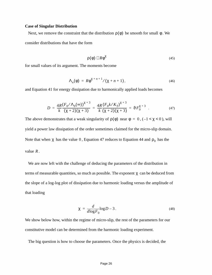
Case of Singular Distribution

Next, we remove the constraint that the distribution be smooth for small . We

consider distributions that have the form

(45)

for small values of its argument. The moments become

, (46)

and Equation 41 for energy dissipation due to harmonically applied loads becomes

. (47)

The above demonstrates that a weak singularity of near , ( ), will

yield a power law dissipation of the order sometimes claimed for the micro-slip domain.

Note that when has the value , Equation 47 reduces to Equation 44 and has the

value .

We are now left with the challenge of deducing the parameters of the distribution in

terms of measurable quantities, so much as possible. The exponent can be deduced from

the slope of a log-log plot of dissipation due to harmonic loading versus the amplitude of

that loading

. (48)

We show below how, within the regime of micro-slip, the rest of the parameters for our

constitutive model can be determined from the harmonic loading experiment.

The big question is how to choose the parameters. Once the physics is decided, the

ρ φ( ) φ

ρ φ( ) Rφχ≅

Λn φ( ) Rφχ n 1+ + χ n 1+ +( )⁄=

D4Rk

-------F0 Λ0 ∞( )⁄( )χ 3+

χ 2+( ) χ 3+( )----------------------------------------

4Rk

-------F0k KT⁄( )χ 3+

χ 2+( ) χ 3+( )----------------------------------- ϑF0

χ 3+= = =

ρ φ( ) φ 0= 1 χ 0< <–

χ 0 ρ0

R

χ

χF0logd

dDlog 3–=

exponent is fixed. The hard question is how to determine ( in the case ), ,

and . One strategy would be to devise some other class of experiment with the

intention that these new experiments would further identify the individual parameters that

go into making up . We consider an experiment in which a large force is applied to the

joint and then released:

• the elastic compliance of the overall joint drowns out the deflections due to interface

slip during extension

• after release, the residual displacement is due solely to interface mechanics

This suggests that experiments relating the residual deformation and the amplitude of the

applied load or the displacement during the loading portion of the experiment might help

resolve the problem of identifying the remaining parameters. As shown in Appendix A,

for the case where , the resulting residual deformation is related to the maximum

deformation by

(49)

where is the residual deformation and is the maximum loading. We see that the

parameters , , and group together in the same manner in this problem as they do in

the calculation of dissipation under oscillatory loading.

This suggests that the individual values of ( in the case ), , and do not

matter in the dissipation modeling of the joint; that what matters is the manner in which

these parameters come together to form the quantity . (Note that

the individual values of the parameters will make a difference in the values of the hidden

χ R ρ0 χ 0= k

KT

υ

χ 0=

uR14---

ρ0k2

KT3

-----------

FM2

=

uR FM

ρ0 k KT

R ρ0 χ 0= k KT

ϑ 4Rk

-------k KT⁄( )χ 3+

χ 2+( ) χ 3+( )-----------------------------------=

variables; those values will not be observable from macroscopic scale experiments.)

The above assertion is argued mathematically in Appendix B and supported by a

numerical experiment using parameters as indicated in the following table:

The number of elements and the number of time-steps is gross over-kill for the problem at

hand, but were selected in order to assure that the difference in the predictions of the two

cases was due only to the intrinsic mathematical difference due to selecting different

combinations of , , and that combine to the same value of . The imposed load in

this test case is a sum of sine functions of different period and amplitude

(50)

and is shown in Figure 6. This load was selected to be significantly different from a simple

harmonic loading. In particular, there are significant load reversals on each side of the

zero-crossings.

Table 1: Parameters of two Iwan Models

Fmax Iwan Elements

Time Steps ρ0 k KTResulting Dissipation

Case 1 1.0 50 2000 4.0 0.5 1000 6.66667E-10 2.74149E-10

Case 2 1.0 50 2000 2.0 2.0 2000 6.66667E-10 2.74159E-10

ϑ2ρ0k

2

3KT3

--------------=

R k KT ϑ

F t( ) 12--- t( ) 1

2--- 6t( )sin+

sin =

The resulting time derivatives of the hidden variable are shown in Figure 7. Because

the product of Case 1 is half that of Case 2, the displacements of Case 1 are double

those of Case 2.

Figure 6. Test case using non-sinusoidal applied force

F t( ) 12--- t( ) 1

2--- 6t( )sin+sin

=

t

F t( )

0 2 4 6 8-1

-0.5

0

0.5

1

u

ρ0k

The net force due to the slipping Iwan elements is shown in Figure 8. We see that the

forces of Case 1 are just about half of those of Case 2.

Figure 7. Resulting time derivative of displacement u(t)

u t( )

t

Case 1

Case 2

0 2 4 6 8-2.00e-03

-1.00e-03

0.00e+00

1.00e-03

2.00e-03

The instantaneous energy dissipation is that due to motion of the sliding elements. This

is the product of the forces in Figure 8 times the displacement rates of Figure 7. Those

dissipation rates are shown in Figure 9. The dissipation rates for Cases 1 and 2 are

identical and superpose.

Figure 8. Instantaneous net force from all sliding Iwan elements.

Case 2

0 2 4 6 8-8.00e-07

-3.00e-07

2.00e-07

7.00e-07

Case 1

t

Fsl

idin

g

We conclude from the above discussion that in the domain of small applied loads, the

distribution behaves as a fractional negative power of its argument. Further, though

the model parameters , , and are defined uniquely, we are free to select the model

parameters, , , and arbitrarily so long as

(51)

and the dissipative nature of the system will be preserved. Note that varying the values of

, , and does change the magnitudes of the hidden displacements and .

Note that the above discussion applies to the region of small applied forces, where clean

data on the force-displacement relationships is hard to obtain but where dissipation versus

amplitude data is available. It is in the correspondingly small values of that

Figure 9. Resulting dissipation rates are identical for both cases.

Cases 1 & 2

Dis

sip

atio

n R

ate

t0 2 4 6 8-1.00e-10

0.00e+00

1.00e-10

2.00e-10

3.00e-10

4.00e-10

ρ φ( )

χ υ K1

R k KT

4Rk

-------k KT⁄( )χ 3+

χ 2+( ) χ 3+( )----------------------------------- υ=

R k KT u xk{ }

φ ρ φ( )

behaves as a power of its argument.

Large Force ResponseIt is shown above how experiments involving small oscillatory loads can provide

information on for small values of its argument through consideration of dissipation.

Here, we see how estimates for for large values of its argument can be obtained

through considerations of a different sort.

One expects the force-displacement curve for large monotonic loading to look

something like that in the following figure. In the regime of small loads (micro-slip), the

curve is nearly linear and little information can be deduced from the curvature. More

importantly, in the region of small loads, there is no practical method to deduce from

the observable joint quantities, and . Though, in principle, one could solve the

following equation

(52)

ρ φ( )

ρ φ( )

u

F

Figure 10. Force-displacement curve for large monotonic loading

Large Partial Slip

Micro-Slip

u t( )

U F

u t( ) U t( ) F K1⁄–=

for , evaluation of that equation would involve looking for nearly in-perceptible

differences between experimental values.

The problem simplifies a bit in the region of large displacements - well beyond the

region of micro-slip. In that region, one could use the above equation to get realistic

values of from and . We may now plot versus and evaluate the curvature of

the plot numerically to estimate for large values of its argument via Equation 31.

Note that in these experiments is no longer a hidden variable.

Note also that the model parameter appears in Equation 31 and is still to be assigned a

unique value.

Model Parameters

Selecting Parameters

The model parameters and are defined uniquely in terms of dissipation experiments

at low amplitude. The parameter is uniquely determined from small amplitude force-

displacement experiments. The remaining parameters, , , and , can be chosen

arbitrarily to match the dissipation at small force amplitude so long as Equation 51 is

satisfied. This arbitrariness is disturbing. Also, it would be desirable to define over

the full range of its argument. These issues can be resolved in the following manner.

1. Set . This is equivalent to making the change of variables in Equations 28 and 31.

2. Equation 31 can now be used unambiguously to determine a plot of versus for

large values of .

3. Let be the minimum value of for which the above process yields reliable values

of .

u

u t( ) U F F u

ρ φ( )

u

k

χ υ

K1

R k KT

ρ φ( )

k 1= ρ φ( ) ρ φ k⁄( ) k2⁄=

ρ φ( ) φφ

φ φρ

4. Select so that matches the value obtained from Equation 31.

5. Use Equation 51 to determine .

6. Use for and use obtained from Equation 31 for .

Discretization of the Model

The continuous Iwan model is characterized by the two numbers and and the

function . Here we discuss how one may approximate the continuous Iwan model,

whose parameters can be determined by the methods above, by a finite system of discrete

Iwan elements.

Discretization of the continuous Iwan system is most economically done by using only

as many Iwan elements as necessary. Lets assume that the experiments we contemplate

simulating involve loads for which is an upper bound. One can employ Equation 30 to

plot versus for monotonically applied loads and thereby to find a corresponding .

The constitutive equation may now be evaluated numerically by breaking the domain of

integration into the two domains and . The Iwan model

becomes

. (53)

We now approximate the above integral by a summation over discrete points

R Rφχ

ρ φ( )

KT

ρ φ( ) Rφχ= φ φ< ρ φ( ) φ φ<

KT k

ρ φ( )

FM

F u uM

0 ∞,( ) 0 kuM,( ) kuM ∞,( )

F k u x φ( )–( )ρ φ( ) φ ku ρ φ( ) φd

kuM

∞

∫+d

0

kuM

∫=

k u x φ( )–( )ρ φ( ) φ u KT k ρ φ( ) φd

0

kuM

∫–+d

0

kuM

∫=

. (54)

When Equation 54 is substituted into Equation 53, one obtains

(55)

where dependence on time is shown explicitly and is the quantity in the brackets in

Equation 53.

Numerical experiments for the case , presented below, have been reasonably

successful with a uniform distribution of sample points. Slightly negative values of

might be well suited by a distribution consistent with some other quadrature strategy.

An example of the above strategy is presented in Appendix B.

ρ φ( ) ρ φ( )δ φ φj–( )∆φj∑≅

F t( ) k ρ φj( ) u t( ) xj t( )–[ ]∆φj u t( )KTˆ+∑=

KTˆ

χ 0=

χ

Conclusions

1. A number of plausible reasons can be put forth for why the Goodman analysis of micro-slip in joints fails quantitatively and yet is vindicated in predicting a power-law relationship between applied lateral force and energy dissipation.

2. Iwan elements do appear to be natural candidates for joint models since they possess the physical qualities of elasticity and slip associated with joint mechanics.

3. Distributions of Iwan elements can be devised that will reproduce the power-law behavior at small amplitude that is found experimentally.

4. Experimental data from dissipation measurements at small loads and force-displacement measurements at large load can be used to determine all the necessary model parameters.

5. Numerical simulation with the distributions of Iwan elements can be performed quickly and efficiently.

References

1. Ungar, Eric E., “Energy dissipation at structural joints; mechanisms and magnitudes”,

Technical Documentary Report No. FDL-TDR-64-98, Air Force Flight Dynamics

Laboratory, Wright-Patterson Air Force Base, Ohio, 1964.

2. Ungar, E.E., “The status of engineering knowledge concerning the damping of built-up

structures”, Journal of Sound and Vibration, 26, 1973, pp. 141-154.

3. Lebedev, N. N., Special Functions and Their Applications, rev. English ed. New York:

Dover, 1972.

4. Mindlin, R.D., “Compliance of elastic bodies in contact”, J. Appl. Mech., 16, 1949,

259-268.

5. Cattaneo, C., “Sul contatto di due corpi elasticiti: distribuzione locale degli sforzi”,

Rendiconti dell’ Accademia naxionale dei Lincei, 27, Ser. 6, 1938, p. 214

6. Johnson, K.L., Contact mechanics, Cambridge University Press, 1985

7. Johnson, K.L., ‘Energy dissiopation at spherical surfaces in contact transmitting

oscillating forces”, Journal of Mechanical Engineering Sciences, 3, 1961, p 362

8. Goodman, L. E., “A review of progress in analysis of interfacial slip damping”,

Structural Damping, papers presented at a colloquium on structural damping held at the

ASME annual meeting in Atlantic City, NJ, December, 1959, edited by Jerome E.

Ruzicka, pp. 35-48.

9. Iwan, W. D., “On a class of models for the yielding behavior of continuous composite

systems”, Journal of Applied Mechanics, 89, 1967, pp. 612-617.

10. Sanliturk, K. Y. and D. J. Ewins, “Modelling two-dimensional friction contact and its

application using harmonic balance method”, Journal of Sound and Vibration, 193,

1996, pp. 511-523.

11. Gaul, L. and J. Lenz, “Nonlinear dynamics of structures assembled by bolted joints”,

Acta Mechanica, 125, 1997, pp. 169-181.

12. Rabinowitcz, E., Friction and Wear of Materials, John Wiley and Sons, New York,

1995, pp 69-71.

13. Pierre, C., A. A. Ferri, and E. H. Dowell, “Multi-harmonic analysis of dry friction

damped systems using an incremental harmonic balance method”, Journal of Applied

Mechanics, 52, 1985, pp. 958-964.

14. Sanliturk, K. Y., M. Imregun, and D. J. Ewins, “Harmonic balance vibration analysis

of turbine blades with friction dampers”, Journal of Vibration and Acoustics, 119, 1997,

pp. 96-102.

15. Smallwood, D. O., D. L. Gregory, and R. G. Coleman, “Damping Investigations of a

Simplified Frictional Shear Joint”, Preceedings of the 71st Shock and Vibration

Symposium, Alexandria VA, Nov. 2000.

16. Menq, C.-H., J. Bielak, and J. H. Griffin, “The influence of microslip on vibratory

response, part 1: a new microslip model”, Journal of Sound and Vibration, 107, 1986,

pp. 279-293.

This Page Intentionally Left Blank

Appendix A: The Residual Slip Experiment

We next consider the slip captured after a monotonically applied force which achieves

its maximum at a value . Equation 30 provides the relationship between that applied

force and the resulting displacement . (Recall that is a hidden variable; ) The

distribution of slider displacement is

(A1)

where is the moment at which the applied load reaches its maximum. Of course, the

imposed displacement associated with the elasticity of the overall joint disappears when

the applied load is removed and a residual displacement associated with interface slip

remains. The problem is illustrated in the following figure.

FM

u1 u1 u1 1«

x φ t1,( ) u1 φ k⁄( ) for φ ku1<–=

x φ t1,( ) 0 for ku1 φ<=

t1

uR

U

F

Figure A1. The problem of residual deformation.

Let’s solve for in terms of the applied load.

At time , after the load is removed, there is no load in the soft spring and the residual

displacement is . At that time, the distribution of slider displacement is

. (A2)

The slip values for time and are shown in Figure A2.

Substituting zero-force into Equation 28, we find an expression to solve for in terms of

(A3)

uR

t2

uR

x φ t2,( ) uR φ k for φ k<⁄u1 uR–

2----------------- +=

x φ t2,( ) u1 φ k⁄( ) for ku1 uR–

2----------------- φ ku1< <–=

x φ t2,( ) 0 for ku1 φ<=

t1 t2

xφ

t,(

)

φ

x φ t1,( )

x φ t2,( )

φ x,( ) k2--- u1 uR–( ) 1

2--- u1 uR+( ),

=

φ ku1=

Figure A2. Slip distribution during the forward motion of the joint and after force on the joint has been released.

u1

uR

u1

uR

uRKT kuR φ+( )ρ φ( ) φ ku1 φ–( )ρ φ( ) φdφ

ku1

∫+d0

φ

∫=

where .

When we approximate for small , we may solve for in terms of

(A4)

For very small and ,

. (A5)

Finally, we exploit the assumption of small slip (Equation 40) to observe that

(A6)

so that residual displacement can be expressed in terms of the applied load

. (A7)

Note that the quantity in parenthesis is the same combination of parameters that occurs in

the expression for dissipation resulting from harmonic tangential loading.

φ k2--- u1 uR–( )=

ρ φ( ) ρ0= φ u1 uR

u1 uR–2

ρ0k-------- 4ρ0KTuR 2 ρ0kuR( )2

–[ ]+=

u1 uR

u1 2KTuR

ρ0k2

------------- 1 2⁄

=

u1 FM KT⁄=

uR

uR14---

ρ0k2

KT3

-----------

FM2

=

Appendix B: Significance of the Dissipation Parameter

In Equation 47, relates the rate of dissipation due to harmonic loading to a power of

the amplitude of the applied load. Here we establish, that where the “small force”

assumption is employed so that the distribution function can be represented

adequately by its behavior near zero (Equation 45) and by the integral defining

(Equation 38), it does not matter how the parameters , , and are chosen so long as

the correct ratio for is achieved. In the next appendix, it is shown

how to determine the appropriate values of from finite element calculation.

We consider two distinct Iwan systems. The first is characterized by the parameters ,

, and and the second by the parameters , , and . Re-using the scalars , ,

and , we assume the relationships

. (B1)

The symbols , , and are reused here because of the small size of the Greek alphabet

and have nothing to do with their earlier use in the body of this monograph.

Each system is subject to the identical load history where is always less than

some and the hidden displacements are expressed to first order as

(B2)

The integrands and range over and , respectively. Setting

(B3)

ϑ

ρ φ( )

KT

k KT R

ϑ 4Rk

-------k KT⁄( )χ 3+

χ 2+( ) χ 3+( )-----------------------------------=

ϑ

k

KT R k KT R α β

γ

KT αKT=

k βk=

R γR=

α β γ

F t( ) F t( )

FM

u t( ) F t( ) KT⁄= u t( ) F t( ) KT⁄=

φ φ 0 kuM,( ) 0 kuM,( )

φkuM----------

φkuM----------=

from which follows

. (B4)

We now relate the slider displacements and of the two systems. Say that

instantaneously the following holds

. (B5)

We shall show that the time derivatives of each of these quantities are such as to maintain

compliance with Equation B5. The sliders are either moving or not and we consider each

case individually. Say the slider at is not moving then

(B6)

and we see that also. On the other hand, say that the slider at is moving,

then

(B7)

and

. (B8)

Since the displacement of all sliders begin’s with the same initial value (zero), we see that

. (B9)

We now examine the instantaneous rate of dissipation

(B10)

φkuM

kuM----------φ β

α---φ= =

x φ t,( ) x φ t,( )

x φ t,( ) 1α---x φ t,( )=

φ x· φ t,( ) 0=( )

k u x φ t,( )– φ βα---k u x φ t,( )–

βα---φ k u x φ t,( )– φ<⇒<⇒<

x·φ t,( ) 0= φ

k u x φ t,( )– φ βα---k u x φ t,( )–

βα---φ k u x φ t,( )– φ=⇒=⇒=

x· φ t,( ) u· t( ) 1α---x· φ t,( )⇒ 1

α---u· t( ) x

·φ t,( )⇒ 1

α---x· φ t,( )= = =

x φ t,( ) 1α---x φ t,( )≡

d t( ) x· φ t,( )φρ φ( ) φd

0

kuM

∫ Ru· t( ) ψ χ· φ t,( )( )φ1 χ+

φd

0

kuM

∫= =

where is a characteristic function of its argument, defined as

. (B11)

Similarly,

. (B12)

The above asserts that the two systems will indistinguishable in their dissipation

properties so long as

. (B13)

Satisfaction of Equation B13 is equivalent to the assertion that the systems will be

indistinguishable so long as they are associated with the same value of

. (B14)

ψ χ· φ t,( )( )

ψ ξ( ) 0 when= ξ 0=

ψ ξ( ) 1 when= ξ 0≠

d t( ) x·φ t,( )φρ φ( ) φd

0

kuM

∫ Ru·

t( ) ψ χ·φ t,( )( )φ

1 χ+φd

0

kuM

∫= =

γβ---

βα--- 3 χ+

Ru· t( ) ψ χ· φ t,( )( )φ1 χ+

φd

0

kuM

∫ γβ---

βα--- 3 χ+

d t( )= =

γβ---

βα--- 3 χ+

1=

ϑ

ϑ 4R

k-------

k KT⁄( )χ 3+

χ 2+( ) χ 3+( )-----------------------------------

γβ--- β

α--- 3 χ+ 4R

k-------

k KT⁄( )χ 3+

χ 2+( ) χ 3+( )-----------------------------------

ϑ= = =

Appendix C: Example Finite Element Calculation

If one has a prototype of an isolated joint, one can perform harmonic experiments at

different amplitudes to obtain a linear plot of force versus displacement (from which

can be obtained) and a log-log plot of dissipation versus force amplitude (from which

and can be obtained). From and , one constructs an Iwan model in the manner

described in the body of this monograph.

Alternatively, one can devise a detailed finite element mesh for the joint and solve the

fine-scale contact problem assuming a reasonable friction law, usually Coulomb friction.

The following example calculations were performed using the Sandia finite element code

JAS on a mesh created with the help of the Sandia code CUBIT. The joint mesh is

indicated in Figures C1 through C3. Approximately three hundred thousand degrees of

freedom were employed in this model.

K1

χ

ϑ ϑ χ

Figure C1. A mesh of a simple lap joint. The rounded rods on the top and bottom are portions of rigid rollers pushing the laps together.

Figure C2. A magnified view of the mesh of the previous figure.

Vertical loads of 1.78 x108 dynes (400 pounds force) are applied by rollers to push the

laps together and the laps are then pulled apart under displacement control. The force

Figure C3. A further magnified view of the finite element mesh.

resulting displacements curve is plotted in the following figure.

The plot of dissipation versus applied force is shown in the following figure,

Figure C4. The force displacement curve can be matched reasonably well with a straight line. The slope of this line is .K1

displacement (cm.)

Fo

rce

(dyn

e)

0 1e-05 2e-050

2e+06

4e+06

6e+06

8e+06

Joint Force vs. Displacement

F 2.9x1011dyne

cm-----------u=

Having the two parameters and , we now have the necessary parameters to create

an appropriate Iwan model

Figure C5. Dissipation associated with monotonically applied force is used to deduce the dissipation ratio .ϑ

Applied Force (dyne)

Dis

sip

atio

n (

dyn

e cm

)

0 2e+06 4e+06 6e+060

0.05

0.1

Dissipationϑ 3.5x10

22– dyne cm

dyne3

--------------------=

K1 ϑ

Distribution

1 MS 9018 Central Technical Files, 9845-12 MS 0899 Technical Library, 96161 MS 0612 Review & Approval Desk,9612

For DOE/OSTI

1 MS 0841 Bickel, Thomas C 91001 MS 0824 Ratzel, Arthur C 91101 MS 0847 Morgan, Harold S 91201 MS 0824 Moya, Jaime 91301 MS 0827 McGlaun, J Michael 91401 MS 9042 Kawahara, Wendell 87251 MS 9042 Dawson, Dan 87251 MS 9042 Antoun, Bonnie 87251 MS 0557 Baca, Thomas J 91251 MS 0557 Gregory, Danny Lynn 91251 MS 0847 Martinez, David R. 91245 MS 0847 Dohner, Jeffery 91241 MS 0847 Smallwood, David 912410 MS 0847 Segalman, Daniel J. 9124

1 Prof. Lawrence BergmanUniv. of IllinoisAero/Astro Engr.Urbana, IL 61801

1 Prof. Alexander F. Vakakis Department of Mechanical

& Industrial Engineering 104 Mechanical Engineering Building,

MC-244 1206 West Green Street Urbana, IL 61801

1 Prof. Xiaomin Deng Department of Mechanical Engineering University of South Carolina Columbia, SC 29208

1 Prof. Lee PetersonUniversity of Colorado at BoulderCampus Box 429Boulder, CO 80309-0429

1 Prof. K.C. ParkUniversity of Colorado at BoulderCampus Box 429Boulder, CO 80309-0429

1 Dr. Marie LevineJet Propulsion Laboratory (JPL)Science and Technology

Development Section 4800 Oak Grove DrivePasadena, CA 91109-8099

1 Prof. Edward J. BergerDept. Mech. & Industrial Engr.University of CincinnatiPO Box 210072Cincinnati, OH 45221-0072

an initial overview of iwan modeling for mechanical...

Documents