an improved method for the identification and … improved meth… · an improved method for the...
TRANSCRIPT

An Improved Method for the Identification and Inversion
of Multi-Mode Rayleigh Surface Wave Dispersion Collected From Non-Uniform Arrays Utilizing A Moving Source
Approach
A Dissertation
Presented for the
Doctor of Philosophy Degree
The University of Memphis
Scott Stovall
May 2010

ii
Dedication
I would like to dedicate this dissertation to my wonderful wife Koreena who has and
still supports my pursuit of my education. You have stood by my side all these years, and
I greatly appreciate it. I love you.
iii
Acknowledgments
I would like to thank Dr. Shahram Pezeshk for his dedication and support throughout
my educational endeavor. You have been a great mentor and a friend and I will always
appreciate what you have helped me accomplished. Thank you.
I also would like to thank my committee members, Professors: David Arellano,
Charles Camp, Roger Meier, and Jose Pujol for all their help in making this dissertation
possible. I would like to express my gratitude for all you members have done for me.
Thank you.
I would like to thank all my family and friends whom have supported me through
during this long period. Your support is greatly appreciated and will never be forgotten.
I would also like to thank Rick Voyles and Robert Jordan from the machine shop.
Both of you have been instrumental in the success of all my field experiments. Without
you guys a lot of this would not have been possible. Thank you.
This material is based upon work supported by Tennessee Department of
Transportation (Project #: ED-08-22534-00) for funding this project. Any opinions, and
conclusions or recommendations expressed in this material are those of the author and do
not necessarily reflect the views of the Tennessee Department of Transportation.

iv
Abstract
Stovall, Scott. Ph.D. The University of Memphis, May 2005. An Improved Method for the Identification and Inversion of Multi-Mode Rayleigh Surface Wave Dispersion Collected From Non-Uniform Arrays Utilizing A Moving Source Approach. Major Professor: Shahram Pezeshk
An improved method using a moving source approach is utilized in the analysis of
Rayleigh surface waves for the accurate identification of higher mode propagation used
in inversion. Two non invasive surface wave methods, Multi- station Analysis of Surface
Waves (MASW) and Refraction Microtremor (ReMi) were used for the construction of
composite dispersion curves representing the relationship of Rayleigh phase velocity (VR)
with frequency. Multiple tests were executed with source offsets increasing with each
successive test in order to account for near field effects and higher mode attenuation
levels. The resulting dispersions were combined to form a composite dispersion which
effectively maps all participating modes of propagation. The inversion was executed
using a genetic algorithm (GA) which takes advantage of the Rayleigh forward problem.
The results show good ability to identify intermediate high and low velocity layers and
agree well with downhole results.

v
Table of Contents
Dedication………………………………………………………………………………..ii
Acknowledgments……………………………………………………………………….iii
Abstract……………………………………………………………………………….….iv
List of Tables……………………………………………………………………………viii
List of Figures…………………………………………………………………………….ix
CHAPTER 1. Introductio
Chapter 1. Introduction.................................................................................................... 1
1.1 Introduction ............................................................................................................. 1
1.2 Research Goal ......................................................................................................... 2
1.3 Dissertation overview ............................................................................................. 3
Chapter 2. Literature Review .......................................................................................... 4
2.1 Dynamic Soil Properties ......................................................................................... 4
2.2 Seismic Waves ........................................................................................................ 8
2.3 Plane Waves .......................................................................................................... 10
2.4 Surface Wave Dispersion ...................................................................................... 12
2.5 Rayleigh Waves in Homogeneous Media ............................................................. 15
2.6 Rayleigh Waves in Layered Media ....................................................................... 18
2.7 Rayleigh Waves in a Visco-elastic Heterogeneous Media ................................... 23
2.8 Rayleigh Wave Dispersion Relationship .............................................................. 24
2.9 Rayleigh Wave Modes .......................................................................................... 30
2.10 Rayleigh Wave Attenuation ................................................................................ 40

vi
2.11 Inversion ............................................................................................................. 42
Chapter 3. Rayleigh Surface Wave Measurements ..................................................... 46
3.1 Spectral Analysis of Surface Waves ..................................................................... 46
3.2 Multi-Channel Analysis of Surface Waves ........................................................... 48
3.3 Regression Line Slope Method ............................................................................. 49
3.4 Frequency Wavenumber Method .......................................................................... 53
3.5 Refreaction Microtremor ...................................................................................... 55
3.6 Source Methods .................................................................................................... 57
Chapter 4. Testing and Equipment ............................................................................... 59
4.1 MASW Testing and Equipment ............................................................................ 59
4.2 ReMi Testing and Equipment ............................................................................... 65
4.3 Downhole Testing and Equipment........................................................................ 67
Chapter 5. Signal Processing ......................................................................................... 76
5.1 Frequency Resolution ........................................................................................... 76
5.2 Welch’s Averaged Modified Periodogram ........................................................... 77
5.3 Coherency ............................................................................................................. 78
5.4 Apertures ............................................................................................................... 78
5.5 Spatial Aliasing ..................................................................................................... 81
5.6 Wavenumber Spectrum ......................................................................................... 84
5.7 Higher-Mode Resolution ...................................................................................... 92
5.8 Downhole Arrival Times .................................................................................... 102
5.9 Downhole Velocity Determination ..................................................................... 103

vii
Chapter 6. Experimental Results................................................................................. 108
6.1 Results for Covington, TN .................................................................................. 108
6.2 Results for Hayti, Missouri ................................................................................. 122
Chapter 7. Conclusions ................................................................................................. 133
7.1 Recommendations for Future Research .............................................................. 133
References ...................................................................................................................... 135
Appendix ........................................................................................................................ 170

viii
List of Tables
Table 1. Soil profile-Case 1 ............................................................................................ 25
Table 2. Soil profile-Case 2 ............................................................................................. 27
Table 3. Soil profile-Case 3 ............................................................................................. 28
Table 4. Soil profile-Case 4 ............................................................................................. 29
Table 5. Computed layer velocity as a function of source offsets, V1 = 785.7
ft/sec and V2 = 726 ft/sec. ............................................................................ 106
Table 6. Layer velocity as a function of source offsets, V1 = 1000 ft/sec and V2 =
726 ft/sec. ..................................................................................................... 106

ix
List of Figures
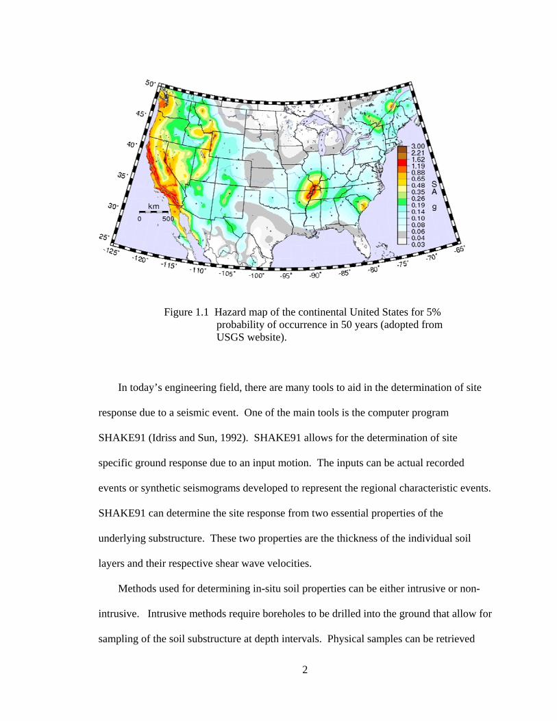
Figure 1.1 Hazard map of the continental United States for 5% probability of occurrence in 50 years (adopted from USGS website). ................................... 1
Figure 2.1 Hysteresis loop representing the stress-strain behavior of a soil undergoing cyclic loading. ............................................................................... 5
Figure 2.2 Backbone curve G plotted with maximum shear modulus Gmax. ................... 6
Figure 2.3 Modulus reduction curve. ................................................................................. 7
Figure 2.4 Particle motions caused by P and S body waves (from Kramer, 1996). ......... 9
Figure 2.5 Particle motion caused by Love and Rayleigh surface waves (from Kramer, 1996). ............................................................................................... 10
Figure 2.6 Plane waves of constant phase propagating in the direction of k. (Adopted from Johnson and Dudgeon, 1993). ............................................... 12
Figure 2.7 Supersposition of two harmonic waves close in frequency and wavenumber (solid line). The dashed curve is the envelope of the modulated wave (adopted from Pujol, 2003) ................................................ 13
Figure 2.8 Superposition of an infinite number of harmonic waves close in frequency and wavenumber. Maximum peaks values for envelope are indicated by the plus signs and the peak of the carrier wave indicated by the circles. Each subplot is a for a fixed value of t. All t values are equally spaced (from Pujol, 2003) ................................................................. 14
Figure 2.9 Relation between Poison’s ratio v and wave velocity propagation. (From Richart et al., 1970). ........................................................................... 17
Figure 2.10 Amplitude ratio vs. dimensionless depth for horizontal and vertical Rayleigh wave displacements for various values of Poisson’s ratio (From Richart et al., 1970). ........................................................................... 18
Figure 2.11 Rayleigh wave penetration depth as a function of frequency f for normalized displacements. ............................................................................. 25
Figure 2.12 Dispersion curve for normally dispersive medium (Case 1). ....................... 26
Figure 2.13 Dispersion curve for Case 2 soil profile with high velocity layer sandwiched between two lower velocity layers. ............................................ 27
Figure 2.14 Dispersion curve for Case 3 soil profile with low velocity layer sandwiched between two higher velocity layers. .......................................... 28

x
Figure 2.15 Dispersion curve for Case 4 soil profile with low velocity layer sandwiched between two higher velocity layers resulting in a jump in the dispersion curve. ...................................................................................... 30
Figure 2.16 Mutli-mode dispersion curves for Case 1. Modes 1 through 4 are represented by blue, green, red, and cyan open circles, respectively. ........... 32
Figure 2.17 Displacement eigenfunctions for first three modes of Case 1 at 40 Hz. .................................................................................................................. 33
Figure 2.18 Mutli-mode dispersion for Case 2. Modes 1 through 4 are represented by blue, green, red, and cyan open circles, respectively. ........... 35
Figure 2.19 Displacement eigenfunctions for first three modes of Case 2 at 40 Hz. .................................................................................................................. 36
Figure 2.20 Mutli-mode dispersion for Case 3. Modes 1 through 4 are represented by blue, green, red, and cyan open circles, respectively. ........... 37
Figure 2.21 Displacement eigenfunctions for first three modes of Case 3 at 40 Hz. .................................................................................................................. 38
Figure 2.22 Displacement eigenfunctions for first three modes of Case 3 at 85 Hz. .................................................................................................................. 38
Figure 2.23 Case 4 Mutli-mode dispersion. Modes 1 through 4 are represented by blue, green, red, and cyan open circles, respectively. .................................... 39
Figure 2.24 Displacement eigenfunctions for first three modes of Case 4 at 40 Hz. .................................................................................................................. 40
Figure 2.25 Displacement eigenfunctions for first three modes of Case 4 at mode jump. .............................................................................................................. 40
Figure 2.26 Geometric spreading function for interpreting geometric attenuation in a heterogeneous media. .............................................................................. 42
Figure 3.1 CSR (top) and CMP (bottom) testing procedures. (Adopted from Rix 2000). ............................................................................................................. 48
Figure 3.2 MASW array setup for uniform (top) and non-uniform (bottom) sensor spacing. ............................................................................................... 49
Figure 3.3 Phase difference as a function of distance (open circles) and unwrapped phase angles (solid circles). ........................................................ 51

xi
Figure 3.4 Dual mode phase unwrapping using RLS. Propagating wavenumbers are represented by solid lines and unwrapped phase angles by circles connected by solid line. ................................................................................. 52
Figure 3.5 Multi mode phase unwrapping using RLS. Propagating wavenumbers are represented by solid lines and unwrapped phase angles by circles connected by solid line. ................................................................................. 53
Figure 3.6 Steered response of a plane wave propagating with wavenumber k = 0.7854. ........................................................................................................... 55
Figure 3.7 p-f spectrum obtained from ReMi method using 24 receivers spaced 8 meters apart. ................................................................................................... 57
Figure 4.1 APS Model 400 ELECTRO-SEIS Shaker. ..................................................... 59
Figure 4.2 Force envelope for Model 400 Shaker. .......................................................... 60
Figure 4.3 APS Model 144 Dual-Mode Amplifier. ......................................................... 60
Figure 4.4 Hewlett Packard 33120A Function/Arbitrary Waveform Function Generator. ...................................................................................................... 61
Figure 4.5 SASW_Testing program developed inVEE Pro. ............................................ 62
Figure 4.6 Wilcox 731A Seismic Accelerometer. ........................................................... 62
Figure 4.7 Wilcox P31 Power Unit/Amplifier with optional gain and filter settings. .......................................................................................................... 63
Figure 4.8 CT-100C portable VXIbus mainframe with slotted VT1432A 16-channel 24-bit digitizer. ................................................................................. 64
Figure 4.9 Main Panel of SASW_Testing program. ........................................................ 64
Figure 4.10 Zoomed in view of a waveform plot for a 35-Hz signal. ............................. 65
Figure 4.11 Data acquisition Equipment. From left to right: Computer with VEE Pro software; 33120A Function/Arbitrary Waveform Function Generator; CT-100C portable VXIbus mainframe with slotted VT1432A 16-channel 24-bit digitizer; and 144 Dual-Mode Amplifier. ....... 65
Figure 4.12 4.5 Hz geophone. .......................................................................................... 66
Figure 4.13 DAQLink II with 12-volt battery and power cable. ..................................... 66
Figure 4.14 Vibrascope program displaying recorded traces. ......................................... 67

xii
Figure 4.15 Downhole testing procedure (top), recorded seismic energy traces (bottom). ........................................................................................................ 69
Figure 4.16 Typical VSP constructed from downhole data. ............................................ 70
Figure 4.17 Interval velocities resulting from VSP. ........................................................ 70
Figure 4.18 Shear-wave hammer system used to generate shear-waves. ........................ 71
Figure 4.19 BHG-2 Wall-Lock geophone system. ......................................................... 72
Figure 4.20 BHGC-4 Borehole geophone controller. ..................................................... 73
Figure 4.21 Data acquisition system for downhole testing. ............................................. 73
Figure 4.22 Front panel display of VEE Pro program for downhole testing. .................. 74
Figure 4.23 Zoomed-in view of single channel recording. .............................................. 75
Figure 5.1 Windowing functions with matching kernels for Rectangular (top), Bartlett (middle), and Hanning (bottom) windows. ....................................... 78
Figure 5.2 ASF for a linear array of length 102 ft. with uniform spacing of 3 ft. (solid line), non uniform array x = [0 2 4 7 10 14 20 26 34 42 52 62 72 87 102] ft. (dashed line). ........................................................................... 80
Figure 5.3 Coarray for 102-ft array with uniform 3-ft spacing. ....................................... 82
Figure 5.4 Coarray for 102-ft array with non uniform spacing. ...................................... 83
Figure 5.5 Array smoothing function for uniform and non-uniform arrays. ................... 83
Figure 5.6 Wavenumber spectrum for single mode propagation. .................................... 84
Figure 5.7 One-second window of synthetic time histories for individual Rayleigh wave mode propagation for each receiver in a non-uniform array. Frequency = 5 Hz with k = 0.2 (dashed) and k = 0.75 (solid). ............ 85
Figure 5.8 One-second window of synthetic time histories of mulit-mode, k1 = 0.2 and k2 = 0.75, Rayleigh wave propagation for frequency of 5 Hz for each receiver in a non-uniform array. ...................................................... 85
Figure 5.9 Wavenumber spectrum for multi-mode, k1 = 0.2 and k2 = 0.75, Rayleigh wave propagation for frequency of 5 Hz. ....................................... 86
Figure 5.10 Wavenumber spectrum for multi-mode, k1 = 0.2 and k2 = 0.5, and k3 = 0.75 Rayleigh wave propagation for frequency of 5 Hz. ........................... 87
Figure 5.11 Fourier amplitude spectrum for all experimental frequencies. ..................... 89
xiii
Figure 5.12 Fourier amplitude spectrum for experimental frequencies from 3.75 to 20 Hz. ......................................................................................................... 90
Figure 5.13 Coherency values for experimental frequencies. .......................................... 91
Figure 5.14 Wavenumber spectrum for experimental data (solid line) and synthetic data (dashed line) for 3.75 Hz, K = 0.013. ..................................... 92
Figure 5.15 Dispersion curve for 10-ft offset. ................................................................. 93
Figure 5.16 Wavenumber spectrum for experimental data (solid line) and synthetic data (dashed line) for 18.75 Hz, k = 0.178. .................................... 94
Figure 5.17 Wavenumber spectrum for experimental data (solid line) and synthetic data (dashed line) for 31.25 Hz, k = 0.337. .................................... 95
Figure 5.18 Wavenumber spectrum for experimental data (solid line) and synthetic data (dashed line) for 55 Hz, k = 0.636. ......................................... 95
Figure 5.19 Wavenumber spectrum for experimental data (solid line) and synthetic data (dashed line) for 80 Hz, k = 0.988. ......................................... 96
Figure 5.20 Wavenumber spectrum for experimental data (solid line) and synthetic data (dashed line) for 100 Hz, k = 1.255. ....................................... 96
Figure 5.21 Dispersion curve for 30-ft offset. ................................................................. 97
Figure 5.22 Wavenumber spectrums for frequencies of 27.5 to 45 Hz for 30-ft offset. ............................................................................................................. 98
Figure 5.23 Wavenumber spectrums for frequencies of 55 to 80 Hz for 30-ft offset. ............................................................................................................. 99
Figure 5.24 Wavenumber Spectrums for frequencies 90 to 100 Hz for 30-ft offset. ........................................................................................................... 100
Figure 5.25 Dispersion curve for 30-ft offset with suspected next-higher mode. ......... 101
Figure 5.26 Dispersion curve for 30-ft offset with suspected next two higher modes. .......................................................................................................... 101
Figure 5.27 Example downhole VSP with picked arrival times. ................................... 103
Figure 5.28 Downhole schematic. ................................................................................. 104
Figure 5.29 Downhole ray paths .................................................................................... 105
Figure 6.1 Tennessee Department of Transportation maintenance facility located in Covington, TN. ........................................................................................ 108
xiv
Figure 6.2 Downhole VSP and shear wave velocity chart for Covington, TN (adopted from Ge et al., 2007) ..................................................................... 109
Figure 6.3 Experimental dispersion curve for Covington, TN with 5-ft offset. ............ 110
Figure 6.4 Coherency values as a function of frequency for Covington, TN with 5-ft offset. .................................................................................................... 110
Figure 6.5 Experimental dispersion curve for Covington, TN with a 10-ft offset. ........ 111
Figure 6.6 Coherency values as a function of frequency for Covington, TN with a 10-ft offset. .................................................................................................. 111
Figure 6.7 Fourier amplitude spectrum for MASW test data (blue) and ground noise (red). ................................................................................................... 112
Figure 6.8 Experimental dispersion curve for Covington, TN with 30-ft offset. .......... 113
Figure 6.9 Coherency values as a function of frequency for Covington, TN with a 30-ft offset. .................................................................................................. 113
Figure 6.10 Experimental dispersion curve for Covington, TN with 60-ft offset. ........ 114
Figure 6.11 Coherency values as a function of frequency for Covington, TN with 60-ft offset. .................................................................................................. 115
Figure 6.12 Frequency-slowness spectrum obtained from ReMi for Covington, TN. ............................................................................................................... 116
Figure 6.13 Composite dispersion curves obtained from MASW (open circles) and ReMi (solid circles) for Covington, TN. ............................................... 117
Figure 6.14 Multi mode inversion of MASW/ReMi dispersion for Covington, TN site. Triangles represent experimental phase velocities. Theoretical phase velocities are represented by; 1. Red circles for fundamental mode, 2. Blue x for 2nd mode, 3. Green squares for 3rd mode and 4. Magenta plus signs for 4th mode. ................................................................ 119
Figure 6.15 Velocity profile comparison for Covington, TN site for 100 ft.. ................ 120
Figure 6.16 Velocity profile comparison for Covington, TN site for 165 ft.. ............... 121
Figure 6.17 Test site located near Hayti, Missouri. ...................................................... 122
Figure 6.18 Downhole VSP and shear wave velocity chart for Hayti, Missouri site. ............................................................................................................... 123
Figure 6.19 Experimental dispersion curve for Hayti, Missouri site with a 10-ft offset. ........................................................................................................... 124

xv
Figure 6.20 Coherency values as a function of frequency for Hayti, Missouri site with a 10-ft offset. ........................................................................................ 125
Figure 6.21 Experimental dispersion curve for Hayti, Missouri site with a 30-ft offset. ........................................................................................................... 125
Figure 6.22 Coherency values as a function of frequency for Hayti, Missouri site with a 30-ft offset. ........................................................................................ 126
Figure 6.23 Experimental dispersion curve for Hayti, Missouri site with a 60-ft offset. ........................................................................................................... 127
Figure 6.24 Coherency values as a function of frequency for Hayti, Missouri site with 60-ft offset. .......................................................................................... 127
Figure 6.25 Frequency-slowness spectrum obtained from ReMi for Hayti, Missouri site. ................................................................................................ 128
Figure 6.26 Composite dispersion curves obtained from MASW (open circles) and ReMi (solid circles) for Hayti, Missouri site. ....................................... 129
Figure 6.27 Multi mode inversion of MASW/ReMi dispersion for Hayti, Missouri site. Triangles represent experimental phase velocities. Theoretical phase velocities are represented by; 1. Red circles for fundamental mode, 2. Blue x for 2nd mode, 3. Green squares for 3rd mode and 4. Magenta plus signs for 4th mode. ........................................... 130
Figure 6.28 Velocity profile comparison to 90 ft. for the Hayti, Missouri site. ............ 131
Figure 6.29 Velocity profile comparison to 200 ft. for the Hayti, Missouri site. .......... 132
Figure A.1 Boring log for Covington, TN ..................................................................... 139
Figure A.2 Boring log for Covington, TN ..................................................................... 140
Figure A.3 Boring log for Covington, TN ..................................................................... 141
Figure A.4 Boring log for Covington, TN ..................................................................... 142
Figure A.5 Boring log for Hayti, Missouri .................................................................... 143
Figure A.6 Boring log for Hayti, Missouri .................................................................... 144
Figure A.7 Boring log for Hayti, Missouri .................................................................... 145
1
Chapter 1. Introduction
1.1 Introduction
For a structure to be built and stand the test of time it must have a solid foundation.
There are many natural disasters that can occur at any time and if not prepared for can
result in catastrophic failures. Over the past century engineers have become more aware
of the hazards associated with earthquakes and have been working diligently to best
prepare for them. One of the most studied hazards is the ground response resulting from
an earthquake. Many of today’s structures are not built on rock foundations and many
countries have found it necessary to build up land in order to provide adequate living
space. This creates significant risk levels in areas where seismic hazards are high.
Seismic hazard by definition is the study of expected ground motion due to an
earthquake event. For large scale zones these hazards are displayed in what is referred to
as hazards maps (Figure 1.1). Hazard maps display the earthquake ground motions for
various probabilities of occurrence and are used in building codes for seismic provisions.
These provisions incorporate hazard maps into the design of buildings and other
structures in order that they may withstand the effects of the ground motion induced by
the probable earthquake event. Hazard maps are constructed based on regional geology
and may not represent the actual conditions for a local site. Research has shown that the
upper 100 ft of the underlying soil structure has significant effect on site response due to
a seismic event (NEHRP, 2003).
2
Figure 1.1 Hazard map of the continental United States for 5% probability of occurrence in 50 years (adopted from USGS website).
In today’s engineering field, there are many tools to aid in the determination of site
response due to a seismic event. One of the main tools is the computer program
SHAKE91 (Idriss and Sun, 1992). SHAKE91 allows for the determination of site
specific ground response due to an input motion. The inputs can be actual recorded
events or synthetic seismograms developed to represent the regional characteristic events.
SHAKE91 can determine the site response from two essential properties of the
underlying substructure. These two properties are the thickness of the individual soil
layers and their respective shear wave velocities.
Methods used for determining in-situ soil properties can be either intrusive or non-
intrusive. Intrusive methods require boreholes to be drilled into the ground that allow for
sampling of the soil substructure at depth intervals. Physical samples can be retrieved
3
and tested in the laboratory to determine the soil properties. The boreholes can then be
cased and sensors placed at specific depths to record the arrival times of seismic waves
generated at the ground surface. A velocity profile of the underlying substructure can
then be produced from the recorded arrival times.
Non-intrusive methods use seismic energy propagating along the surface of the
ground to determine the underlying soil layers. Different techniques use different types
of wave energy arriving at sensors located along the ground to determine the in-situ soil
conditions. One of the most popular techniques is the Multi-channel Analysis of Surface
Waves (MASW). The MASW measures the frequency-dependent phase velocities of
Rayleigh surface waves propagating along the ground surface to construct a dispersion
curve. This dispersion curve is then inverted to determine soil properties such as layer
thicknesses and shear-wave velocities.
The MASW technique has become a popular method for soil velocity profiling and
has been shown to provide reliable results (Lai and Rix, 1998; Foti , 2000; Hebeler,
2001; Pezeshk and Zarrabi, 2005; and Boore and Asten, 2008). However, the MASW
method suffers at low frequencies due to high levels of ground noise and from the
presence of multi-mode Rayleigh wave propagation. Research has shown that when a the
soil substructure contains layers where the soil velocity is either higher or lower than the
layers above and below, higher mode Rayleigh surface waves have significant influence
on the resulting dispersion (Mooney and Bolt, 1966; Tokimatsu, 1992; and Lai and Rix,
1998). It is therefore imperative that all participating Rayleigh modes be identified for
reliable determination of in-situ soil conditions.

4
1.2 Research Goal
The goal of this research is to develop a method for the accurate identification of
higher mode Rayleigh surface waves for use in inversion in order to produce reliable
shear wave velocity profiles. A moving harmonic source approach is used to overcome
the problems associated with near-field effects as well as changes in attenuation as a
function of depth. By increasing the source offset, higher mode Rayleigh wave
participation can be seen in the resulting dispersion curve allowing for the identification
of individual propagating modes. The use of multiple modes in inversion helps to
minimize possible solutions to the Rayleigh eigen-problem.
In order to account for the poor signal-to-noise ratios at low frequencies resulting
from the Harmonic source, a combination of the Multichannel Analysis of Surface Waves
(MASW) method along with the Refraction Microtremor (ReMi) method is used to
construct composite dispersion curves to be used in the inversion process. The composite
dispersion curves allow for a much broader frequency range to be investigated for
Rayleigh wave dispersion.
A genetic algorithm is used for inversion to take advantage of the forward solution of
the Rayleigh eigen-problem and allows for a large search space for finding the optimum
solution. The end result is a multi-mode inversion of Rayleigh wave dispersion that
predicts the in-situ soil velocities of an underlying substructure.
1.3 Dissertation overview
This dissertation is organized into seven chapters containing individual sections
relating to specific topics of interest. Chapter 2 introduces some of the important
characteristics of Rayleigh wave propagation and the resulting theories involved in the
5
solution to the Rayleigh eigen-problem. The effects of multi-mode Rayleigh wave
propagation on dispersion are discussed along with the inversion technique used for the
determination of soil layer velocities. Chapter 3 discusses the methods used in the
measurement of Rayleigh surface wave dispersion. The Regression Line Slope (RLS),
Frequency-wavenumber (f-k), and Refreaction Microtremor (ReMi) methods are
discussed, and the accuracy of each method is addressed. Chapter 4 details the testing
procedures and needed equipment for the collection of experimental Rayleigh wave
dispersion along with the procedures used in downhole testing. Chapter 5 explores the
signal processing techniques used in the methods of Chapter 3 and indentifies important
experimental results needed for the achievement of the research goals. Chapter 6 displays
the results of both the experimental testing and inversion of the Rayleigh wave
dispersion. Comparison is made between the shear wave velocity profiles obtained from
downhole testing and that of the Rayleigh wave inversion results. In Chapter 7, the
conclusions of the research goals are discussed and recommendations for future research
are suggested.
6
Chapter 2. Literature Review
Rayleigh wave propagation is a complex problem governed by the in-situ conditions
within the underlying substructure. The waves themselves are a combination of multiple
seismic waves that interact due to reflections and refractions caused by layer interfaces.
The properties of the individual layers directly influence the dynamic response of the
seismic waves and the resulting propagation characteristics. The following chapter
discusses these properties and how they are used in the formulation of theoretical
Rayleigh wave propagation. Several techniques for the solution of the theoretical model
are discussed along with the method of inversion used for the determination of in-situ
shear-wave velocities.
2.1 Dynamic Soil Properties
One of the key areas in the study of geotechnical earthquake engineering is the site
response resulting from the cyclic loading of the underlying soil structure. The response
is mainly influenced by the properties of the soil commonly referred to as the dynamic
properties. These dynamic soil properties directly influence the behavior of seismic wave
propagation and the resulting site response. The mechanical behavior of soils is a
function of the strain magnitude experienced under specific stress conditions and can best
be understood from the hysteresis loop shown in Figure 2.1. A hysteresis loop charts the
relationship of induced strain as a function of applied stress under cyclic loading
conditions. The inclination of the hysteresis loop is controlled by the soil stiffness, which
is described by the tangent shear modulus at any point during the loading process. The
general inclination of the hysteresis loop can be approximated by averaging the values of
the tangent shear modulus over the entire loading process resulting in (Kramer, 1996)

7
secc
c
G τγ
= (2.1.1)
where τc and γc are the shear stress and shear strain amplitudes. Changes in strain
amplitude during loading result in changes to the hysteresis loop and subsequently the
secant shear modulus.
Figure 2.1 Hysteresis loop representing the stress-strain behavior of a soil undergoing cyclic loading.
By plotting the locus of points corresponding to the tips of the hysteresis loops for
different strain amplitudes, a curve known as the backbone curve can be plotted with
respect to strain amplitude (Figure 2.2). The slope of the curve measured at the origin
represents the largest value of the shear modulus (Gmax). When strain amplitude is zero,
G and Gmax are equal. As strain amplitude increases the ratio G / Gmax drops. This ratio is
Gtan
Gsecτ
γγc
τc
8
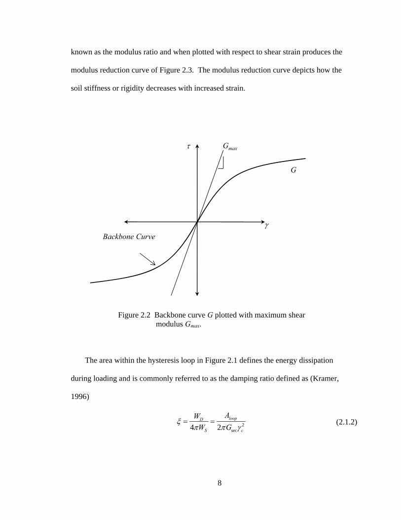
known as the modulus ratio and when plotted with respect to shear strain produces the
modulus reduction curve of Figure 2.3. The modulus reduction curve depicts how the
soil stiffness or rigidity decreases with increased strain.
Figure 2.2 Backbone curve G plotted with maximum shear modulus Gmax.
The area within the hysteresis loop in Figure 2.1 defines the energy dissipation
during loading and is commonly referred to as the damping ratio defined as (Kramer,
1996)
2
sec4 2loopD
S c
AWW G
ξπ π γ
= = (2.1.2)
Backbone Curve
τ
γ
Gmax
G

9
where WD is the dissipated energy, WS is the maximum strain energy, and Aloop is the area
of the hysteresis loop.
Figure 2.3 Modulus reduction curve.
From Equation (2.1.2) it can be inferred that as strain amplitude increases, Gsec will
decrease resulting in an increase in Aloop and thus an increase in damping with increased
strain. In seismology a dimensionless definition is given for energy dissipation known as
the quality factor Q (Aki and Richards, 1980):
1( )
2 ( )Q ω
ξ ω= (2.1.3)
It should be noted that both ξ and Q assume a material under linear stress-strain
conditions. Later sections will show how this dissipation of energy can have a dramatic
log γ
max
GG
1.0

10
effect on Rayleigh wave propagation. The dynamic soil property most used in site
response is the shear wave velocity defined as (Kramer, 1996)
SS
GVρ
= (2.1.4)
where VS is the shear wave velocity, ρ is the mass density and GS is the shear modulus.
The shear modulus is defined by
2(1 )SEG
v=
+(2.1.5)
where E is the elastic modulus and v is Poisson’s ratio. The shear wave velocity is used
as input for site response programs such as SHAKE91 (Idriss and Sun, 1992). SHAKE91
uses shear wave velocities along with shear modulus reduction and damping curves to
determine ground accelerations based on an equivalent linear elastic analysis.
The compression wave velocity is determined in a manner similar to that of VS
and is expressed as
2B SP
G GVρ+
= (2.1.6)
where GB is known as Lame’s constant. Lame’s parameters are typically identified as λ
and μ, however, to minimize confusion in later sections and maintain consistency GB and
GS, respectively, are used here.
Lame’s parameters are related to the elastic modulus and Poisson’s ratio. GS is
the shear modulus described above and GB is used to describe the effects of dilation on
tensile stress. GB is related to the bulk modulus by

11
2
3B SG K G= − (2.1.7)
where K is defined as
(1 ) 4(1 )(1 2 ) 3 S
v EK Gv v−
= −+ −
(2.1.8)
Inserting Equation (2.1.8) into (2.1.7) GB is expressed by
(1 )(1 2 )BvEG
v v=
+ −(2.1.9)
The above dynamic soil properties directly influence seismic wave propagation used
in the determination of in-situ soil conditions. This will become clear in the following
section, which discusses seismic wave propagation and the fundamental theories involved
for Rayleigh surface wave propagation.
2.2 Seismic Waves
Seismic waves are waves of energy the travel through the earth radiating outward
from their source. A source may be the sudden rupture of rock along a fault line, an
explosion, or any other force imparted in the earth. There are two types of seismic
waves: body and surface waves. Body waves travel in the interior of the earth as opposed
to surface waves that travel along the surface of the earth.
Body waves are composed of P and S waves. P waves, also known as primary or
compression waves, exhibit particle motion in the direction of propagation and mimic a
spring undergoing compression and dilation. S waves, also known as secondary or shear

12
waves, exhibit particle motions perpendicular to the direction of propagation. They can
be divided into SV and SH waves. SV waves are S waves associated with vertical particle
motion perpendicular to the direction of propagation and SH waves are those associated
with horizontal motion (Figure 2.4).
Figure 2.4 Particle motions caused by P and S body waves (from Kramer, 1996).
Surface waves are the result of the interaction of body waves at the surface and at
layer interfaces within the earth. Two types of surface waves of interest are Love and
Rayleigh waves. Love waves, first introduced by Love (1911), are formed from the
interaction of SH waves with a soft layer overlaying a stiffer material resulting in particle
motion that is transverse to the direction of propagation. Rayleigh waves, first introduced
by John Strutt, Lord of Rayleigh, in 1885, are formed from the interaction between P and
SV waves. The horizontal and vertical particle motions combine to form a surface wave

13
with elliptical particle motion in the direction of propagation. This elliptical motion is
the ground roll experienced during earthquakes (Figure 2.5). Rayleigh waves are
attractive because they travel along the surface allowing for the direct measurement of
their propagation characteristics.
Figure 2.5 Particle motion caused by Love and Rayleigh surface waves (from Kramer, 1996).
2.3 Plane Waves
Rayleigh surface wave techniques require that propagating surface waves have
specific characteristics in order for the techniques to be accurate. One of these
characteristics is that the waves be planar. Plane waves are constant frequency waves
14
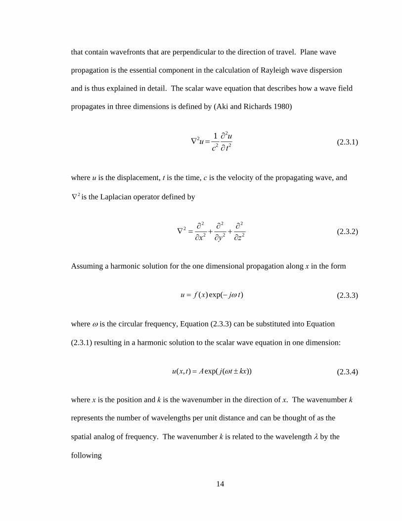
that contain wavefronts that are perpendicular to the direction of travel. Plane wave
propagation is the essential component in the calculation of Rayleigh wave dispersion
and is thus explained in detail. The scalar wave equation that describes how a wave field
propagates in three dimensions is defined by (Aki and Richards 1980)
2
22 2
1 uuc t
∂∇ =
∂ (2.3.1)
where u is the displacement, t is the time, c is the velocity of the propagating wave, and
2∇ is the Laplacian operator defined by
2 2 2
22 2 2x y z
∂ ∂ ∂∇ = + +
∂ ∂ ∂(2.3.2)
Assuming a harmonic solution for the one dimensional propagation along x in the form
( ) exp( )u f x j tω= − (2.3.3)
where ω is the circular frequency, Equation (2.3.3) can be substituted into Equation
(2.3.1) resulting in a harmonic solution to the scalar wave equation in one dimension:
( , ) exp( ( ))u x t A j t kxω= ± (2.3.4)
where x is the position and k is the wavenumber in the direction of x. The wavenumber k
represents the number of wavelengths per unit distance and can be thought of as the
spatial analog of frequency. The wavenumber k is related to the wavelength λ by the
following

15
2k πλ
= (2.3.5)
where λ is the length of the wave propagating along x and is thus termed the wavelength.
Planes of constant phase are perpendicular to the direction of propagation along x (Figure
2.6). If Equation (2.3.4) is a propagating wave, then planes of constant phase move by an
amount δx as time advances by an amount tδ so that
( , ) ( , )u x x t t u x tδ δ+ + = (2.3.6)
Equation (2.3.6) implies that if Equation (2.3.4) is planar then
0t k xωδ δ− = (2.3.7)
and therefore
x ct k
δ ωδ
= = (2.3.8)
where c is the velocity of the plane wave propagating along x. Surface wave
measurement techniques based on spectral analysis use the relationship of Equation
(2.3.8) for determining the phase velocity of propagating waves. However, it must be
understood that Equation (2.3.8) is only applicable to a single sinusoidal propagating
wave. For waves traveling with multiple frequencies and wavenumbers, the dispersion
characteristics must be accounted for.
16
Figure 2.6 Plane waves of constant phase propagating in the direction of k. (Adopted from Johnson and Dudgeon, 1993).
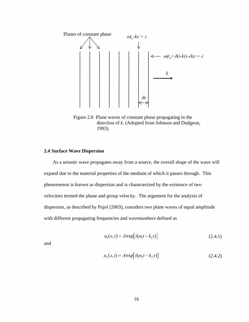
2.4 Surface Wave Dispersion
As a seismic wave propagates away from a source, the overall shape of the wave will
expand due to the material properties of the medium of which it passes through. This
phenomenon is known as dispersion and is characterized by the existence of two
velocities termed the phase and group velocity. The argument for the analysis of
dispersion, as described by Pujol (2003), considers two plane waves of equal amplitude
with different propagating frequencies and wavenumbers defined as
[ ]1 1 1( , ) exp ( )u x t A i t k xω= − (2.4.1)and
[ ]2 2 2( , ) exp ( )u x t A i t k xω= − (2.4.2)
k
δx
ωto-kx = c
ω(to+δt)-k(x-δx) = c
Planes of constant phase
17
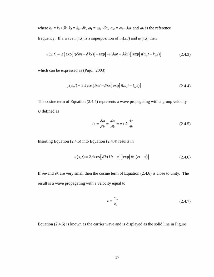
where k1 = ko+δk, k2 = ko−δk, ω1 = ωo+δω, ω2 = ωo−δω, and ωo is the reference
frequency. If a wave u(x,t) is a superposition of u1(x,t) and u2(x,t) then
[ ] [ ]( ) [ ]( , ) exp ( ) exp ( ) exp ( )o ou x t A i t kx i t kx i t k xδω δ δω δ ω= − + − − − (2.4.3) which can be expressed as (Pujol, 2003)
( ) [ ]( , ) 2 cos exp ( )o oy x t A t kx i t k xδω δ ω= − − (2.4.4) The cosine term of Equation (2.4.4) represents a wave propagating with a group velocity
U defined as
d dcU c kk dk dk
δω ωδ
= = = + (2.4.5)
Inserting Equation (2.4.5) into Equation (2.4.4) results in
( ) [ ]( , ) 2 cos exp ( )ou x t A k Ut x ik ct xδ= − −⎡ ⎤⎣ ⎦ (2.4.6)
If δω and δk are very small then the cosine term of Equation (2.4.6) is close to unity. The
result is a wave propagating with a velocity equal to
o
o
ckω
= (2.4.7)
Equation (2.4.6) is known as the carrier wave and is displayed as the solid line in Figure
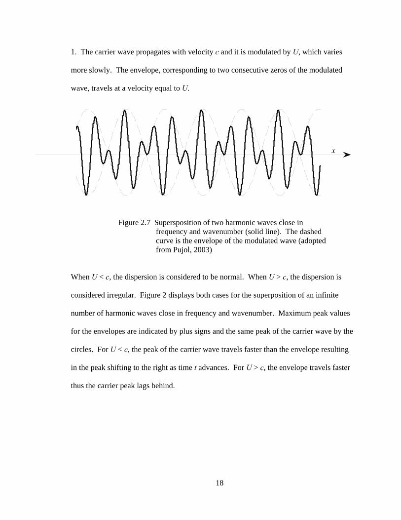
18
1. The carrier wave propagates with velocity c and it is modulated by U, which varies
more slowly. The envelope, corresponding to two consecutive zeros of the modulated
wave, travels at a velocity equal to U.
Figure 2.7 Supersposition of two harmonic waves close in frequency and wavenumber (solid line). The dashed curve is the envelope of the modulated wave (adopted from Pujol, 2003)
When U < c, the dispersion is considered to be normal. When U > c, the dispersion is
considered irregular. Figure 2 displays both cases for the superposition of an infinite
number of harmonic waves close in frequency and wavenumber. Maximum peak values
for the envelopes are indicated by plus signs and the same peak of the carrier wave by the
circles. For U < c, the peak of the carrier wave travels faster than the envelope resulting
in the peak shifting to the right as time t advances. For U > c, the envelope travels faster
thus the carrier peak lags behind.
x

19
Figure 2.8 Superposition of an infinite number of harmonic waves close in frequency and wavenumber. Maximum peaks values for envelope are indicated by the plus signs and the peak of the carrier wave indicated by the circles. Each subplot is a for a fixed value of t. All t values are equally spaced (from Pujol, 2003)
U < c U > c
t

20
For this research, harmonic waves of a individual frequency are generated
resulting in Rayleigh surface wave propagation that follows Equation (2.4.7). This
propagating velocity is known as the phase velocity and from this point will be defined as
RV
kω
= (2.4.8)
where VR is the Rayleigh phase velocity, ω is the frequency of propagation, and k is the
propagating wavenumber. Equation (2.4.8) is commonly referred to as the Rayleigh
dispersion relationship. The term dispersion is used due to the phase velocities
dependence on frequency. For Rayleigh wave measurement techniques, the phase
velocity is the property obtained from field experiments used for the construction of a
dispersion curve. The dispersion curve is used to show the relationship between phase
velocity and frequency of propagating Rayleigh waves, and is used in inversion for
determining in-situ shear-wave velocities. A detailed description of the dispersion curve
and its use is discussed in Section 2.8. The following three sections help to understand
the Rayleigh dispersion relationship by discussing the solution techniques used in
determining the Rayleigh secular function.
2.5 Rayleigh Waves in Homogeneous Media
Rayleigh waves, as discussed in Section 2.2, are surface waves generated from the
interaction of P and SV waves at a free surface. They were first studied in 1885 by Lord
Rayleigh and later described in detail by Lamb (1904). For Rayleigh waves traveling in
a semi-infinite homogeneous isotropic halfspace, the equation of motion in the absence of

21
body forces is described using Navier’s equation in vector notation defined as (Aki and
Richards 1980)
22
2( ) ( )B S SG G Gt
ρ ∂+ ∇ ∇⋅ + ∇ =
∂uu u (2.5.1)
where u is the particle displacement vector, t is the time, ρ is the halfspace density,
( )∇ ⋅ u denotes the divergence of u, 2∇ is the Laplacian operator of Equation (2.3.2), and
GS and GB are Lame’s elastic moduli described in Section 2.1. Lord Rayleigh showed
that for a semi-infinite, linear elastic, homogenous medium with a null stress boundary
condition at the free surface, a solution for the above condition is satisfied by
6 4 2 2 28 (24 16 ) 16( 1) 0K K Kα α− + − + − = (2.5.2)
where α and K are the velocity ratios of shear waves (VS), compression waves (VP), and
Rayleigh waves (VR) defined as
S
P
VV
α = (2.5.3)
R
S
VKV
= (2.5.4)
Equation (2.5.2) is cubic in K2 and real solutions exist for Poisson’s ratio values from 0.0
to 0.5 (Viktorov 1967). Figure 2.9 displays solutions of Equation (2.5.2) for ratios of
VR/VS and VP/VS. The results show that Rayleigh wave velocity within a homogeneous
medium is only slightly lower than that of the shear wave velocity where the compression
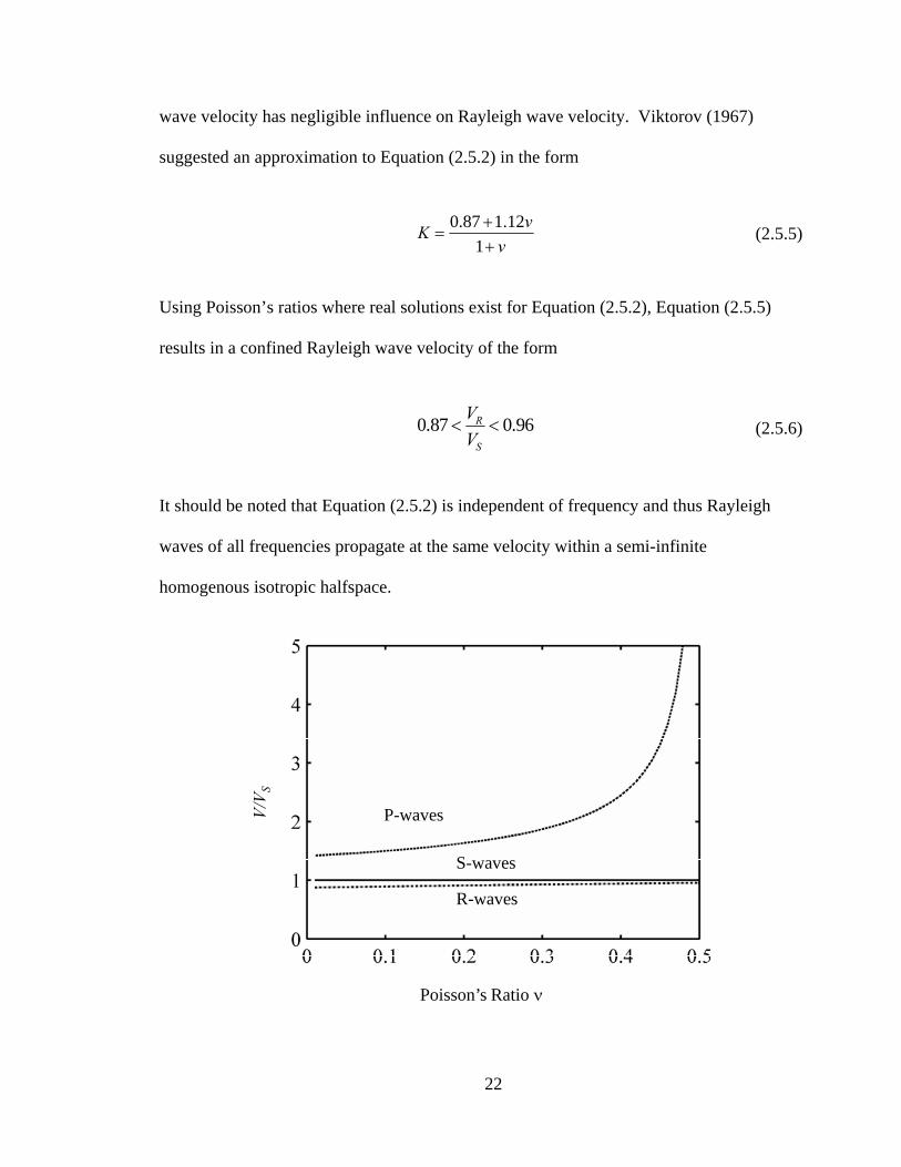
22
wave velocity has negligible influence on Rayleigh wave velocity. Viktorov (1967)
suggested an approximation to Equation (2.5.2) in the form
0.87 1.12
1vK
v+
=+
(2.5.5)
Using Poisson’s ratios where real solutions exist for Equation (2.5.2), Equation (2.5.5)
results in a confined Rayleigh wave velocity of the form
0.87 0.96R
S
VV
< < (2.5.6)
It should be noted that Equation (2.5.2) is independent of frequency and thus Rayleigh
waves of all frequencies propagate at the same velocity within a semi-infinite
homogenous isotropic halfspace.
P-waves
S-waves
R-waves
Poisson’s Ratio ν
V/V S

23
Figure 2.9 Relation between Poison’s ratio v and wave velocity propagation. (From Richart et al., 1970).
Richart et al. (1970) showed the variation of vertical and horizontal Rayleigh wave
displacements within an infinite homogenous isotropic medium to be
2
2
2( ) exp ( ) exp ( )
1
q sq sk kU z zk zk
sk kk
⎡ ⎤ ⎡ ⎤= − − + −⎢ ⎥ ⎢ ⎥⎣ ⎦ ⎣ ⎦+ (2.5.7)
2
2
2( ) exp ( ) exp ( )
1
qs q qkW z zk zk
s k k kk
⎡ ⎤ ⎡ ⎤= − − −⎢ ⎥ ⎢ ⎥⎣ ⎦ ⎣ ⎦+ (2.5.8)
where U(z) and W(z) are the vertical and horizontal displacements as a function of depth
z, k represents wavenumber, and the variables q and s are defined by
22 2
2 1q Kk
α= − (2.5.9)
22
2 1s Kk
= − (2.5.10)
By inserting values of K that satisfy Equation (2.5.2) into Equations (2.5.7) and (2.5.8),
the vertical and horizontal Rayleigh wave displacements as a function of depth can be
determined (Figure 2.10). The resulting horizontal and vertical components of
displacement are out of phase 90 degrees, with the vertical component larger than the
horizontal. This results in an elliptical-retrograde particle motion.

24
It can be seen that the Rayleigh wave displacements become quite negligible as
depth increases, thus material properties at some point will have little if no effect on wave
propagation. This leads to the assumption that a zone of influence exists within the
medium that directly controls wave propagation. This zone has been estimated to extend
to a depth equal to one-half to two-thirds of the wavelength (Sánchez-Salinero, 1987;
Hebeler, 2001). It is this zone of influence that is of special interest for higher mode
Rayleigh wave propagation (Section 2.9). While the preceding discussion helps to
explain some of the characteristics of Rayleigh wave propagation, it does not reflect the
typical conditions present in soils. Most soil substructures contain heterogeneities that
drastically influence Rayleigh wave propagation.
Figure 2.10 Amplitude ratio vs. dimensionless depth for horizontal and vertical Rayleigh wave displacements for various values of Poisson’s ratio (From Richart et al., 1970).
Amplitude at Depth zAmplitude at Surface
Dep
th z
Wav
elen
gth
25
2.6 Rayleigh Waves in Layered Media
For Rayleigh waves propagating in vertically heterogeneous media where the
mechanical properties are assumed to be depth dependent, Navier’s equations take the
following form (Aki and Richards, 1980)
2
22( ) ( ) 2SB
B S S z zdGdGG G G
dz dz z tρ∂ ∂⎡ ⎤+ ∇ ∇⋅ + ∇ + ∇⋅ + ×∇× + =⎢ ⎥∂ ∂⎣ ⎦
u uu u e u e u (2.6.1)
where ez is the unit vector in the direction perpendicular to the free surface and × denotes
the vector product. It can be seen from Equation (2.6.1) that if is there is no change in
Lame’s parameters GB and GS with respect to depth then Equation (2.6.1) becomes
Equation (2.5.1) representing an semi-infinite homogeneous isotropic medium. Aki and
Richards (1980) showed that by assuming a displacement field u(x,t) as
[ ]
[ ]
1 1
2
3 2
( , ( ), ) exp ( ( ) ): 0
( , ( ), ) exp ( ( ) )
u r z k i t k ruu i r z k i t k r
ω ω ω ω
ω ω ω ω
⎧ ⎫= ⋅ −⎪ ⎪
=⎨ ⎬⎪ ⎪= ⋅ ⋅ −⎩ ⎭
u (2.6.2)
where u1,u2, and u3 are the horizontal, transverse, and vertical components of the
displacement field u, i is an imaginary number, ω is the circular frequency of excitation, t
is the time, r is the direction of propagation, and k(ω) is the frequency dependent
wavenumber which is a multi-valued function, substitution of Equation (2.6.2) into
Equation (2.6.1) and writing in matrix form results in

26
[ ]
1 1
2 2
3 32 2
4 4
2
10 ( ) 0( )
( ) ( ) 10 0( ) 2 ( ) ( ) 2 ( )
( ) ( )( ) ( ) ( ) 0 0( ) 2 ( )
0 ( ) ( ) 0
S
B
B S B S
B
B S
kG z
r rk G z
r rd G z G z G z G zr rdz
k G zk z zr rG z G zz k
ω
ω
ωω ζ ω ρ
ω ρ ω
⎡ ⎤⎢ ⎥⎢ ⎥⎡ ⎤ ⎡ ⎤
−⎢ ⎥⎢ ⎥ ⎢ ⎥⎢ ⎥⎢ ⎥ ⎢ ⎥+ += ⋅⎢ ⎥⎢ ⎥ ⎢ ⎥⎢ ⎥⎢ ⎥ ⎢ ⎥−⎢ ⎥⎣ ⎦ ⎣ ⎦+⎢ ⎥⎢ ⎥−⎣ ⎦
(2.6.3)
Where
( )
( )
13 2
24 1
, ( ) , ( )
, ( ) , ( 2 ) ( )
S
B S B
d rr z k G k rd z
d rr z k G G k G rd z
ω ω ω
ω ω ω
⎡ ⎤= −⎢ ⎥⎣ ⎦⎡ ⎤= + +⎢ ⎥⎣ ⎦
(2.6.4)
and ζ(z) is a function of Lame’s parameters:
( )
( )( ) 4
2B S
SB S
G Gz G
G Gζ
+=
+(2.6.5)
By defining f(z) = [r1 r2 r3 r4]T and letting A(z) represent the 4× 4 matrix of
Equation(2.6.3), Equation (2.6.3) can be rewritten as a linear differential eigenvalue
problem
(z) ( ) ( )d z z
dz= ⋅
f A f (2.6.6)
with displacement eigenfunctions ( )1 , ( ),r z k ω ω and ( )2 , ( ),r z k ω ω and stress
eigenfunctions ( )3 , ( ),r z k ω ω and ( )4 , ( ),r z k ω ω subjected to the following boundary
conditions.

27
3 4( , ( ), ) 0, ( , ( ), ) 0 0( , ( ), ) 0
r z k r z k at zf z k as z
ω ω ω ωω ω
= = =→ → ∞
(2.6.7)
For given frequency values ω, specific wavenumber values for k(ω) result in non-
trivial solutions to Equation (2.6.6). These particular values for k(ω) represent the
eigenvalues and the corresponding solutions for rj(z,k(ω),ω) are the eigenfunctions. From
Equation (2.6.3), it can be seen that solutions to the eigenvalue problem are frequency
dependent and thus Rayleigh waves propagating in a layered medium are dispersive.
In its implicit form the Rayleigh dispersion equation is expressed as
[ ]( ), ( ), ( ), 0R B S iG z G z z kρ ω =F (2.6.8)
where ki denotes the the ith mode wavenumber resulting in a solution to the eigenvalue
problem where i = 1: M and M is the total number of possible modes. A solution to
Equation (2.6.8) can be achieved by many different techniques such as finite element,
finite difference, numerical integration, and spectral and boundary element methods.
One of the most common solution techniques is the Thomson-Haskell algorithm.
The algorithm constructs Equation (2.6.8) as the product of layered matrices relating the
displacement and stress components acting at layer interfaces. The roots found in using
the algorithm are the wavenumbers corresponding to the individual modes of
propagation. These wavenumbers are then used for the determination of the
displacement and stress eigenfunctions. However, the algorithm has show numerical
instability at high frequencies (Knopoff, 1964; Dunkin, 1965; Thrower, 1965; Schwab and
Knopoff, 1970; Watson, 1970; Abo-Zena 1979; and Harvey 1981).
28
Kennett (1974) first introduced the method of reflection and transmission
coefficients for the solution of the eigenvalue. It was later improved by Chen (1993) and
Hisada (1994). The method, which is similar to Thomson-Haskell, establishes the
Rayleigh dispersion equation from the construction of reflection and transmission
matrices for the determination of the normal modes in a multi-layered elastic half-space.
This method is very attractive due to its ability to model the constructive interfaces
leading to the formation of Rayleigh wave modes.
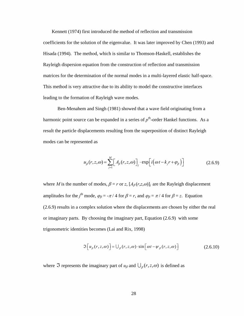
Ben-Menahem and Singh (1981) showed that a wave field originating from a
harmonic point source can be expanded in a series of pth-order Hankel functions. As a
result the particle displacements resulting from the superposition of distinct Rayleigh
modes can be represented as
( )1
( , , ) ( , , ) expM
jjj
u r z A r z i t k rβ β βω ω ω ϕ=
⎡ ⎤⎡ ⎤= ⋅ − +⎣ ⎦ ⎣ ⎦∑ (2.6.9)
where M is the number of modes, β = r or z, [Aβ (r,z,ω)]j are the Rayleigh displacement
amplitudes for the jth mode, ϕβ = -π / 4 for β = r, and ϕβ = π / 4 for β = z. Equation
(2.6.9) results in a complex solution where the displacements are chosen by either the real
or imaginary parts. By choosing the imaginary part, Equation (2.6.9) with some
trigonometric identities becomes (Lai and Rix, 1998)
( , , ) ( , , ) sin ( , , )u r z r z t r zβ β βω ω ω ψ ω⎡ ⎤ ⎡ ⎤ℑ = ⋅ −⎣ ⎦ ⎣ ⎦∪ (2.6.10)
where ℑ represents the imaginary part of uβ and ( , , )r zβ ω∪ is defined as

29
0.5
1 1( , , ) ( , , ) ( , , ) cos ( )
M M
i ji ji j
r z A r z A r z r k kβ β βω ω ω= =
⎧ ⎫⎡ ⎤⎡ ⎤ ⎡ ⎤= ⋅ ⋅ ⋅ −⎨ ⎬⎣ ⎦ ⎣ ⎦ ⎣ ⎦
⎩ ⎭∑∑∪ (2.6.11)
and ψβ is defined as
1 1
1
( , , ) sin4( , , ) tan
( , , ) cos4
M
iiiM
jjj
A r z k rr z
A r z k r
β
β
β
πωψ ω
πω
− =
=
⎡ ⎤⎛ ⎞⎡ ⎤ ⋅ ⋅ −⎢ ⎥⎜ ⎟⎣ ⎦ ⎝ ⎠⎢ ⎥=⎢ ⎥⎛ ⎞⎡ ⎤ ⋅ ⋅ +⎜ ⎟⎣ ⎦⎢ ⎥⎝ ⎠⎣ ⎦
∑
∑
(2.6.12)
If the wavefront in Equation (2.6.10) represents plane wave propagation, then
( , , ) constantt r zβω ψ ω⎡ ⎤− =⎣ ⎦ (2.6.13)
Differentiating Equation (2.6.13) with respect to time
( , , ) 0drr zr dt
βψω ω
∂− ⋅ =
∂(2.6.14)
results in an effective phase velocity
,
ˆ ( , , )( , , )
r
V r zr zβ
β
ωωψ ω
=⎡ ⎤⎣ ⎦
(2.6.15)
where ˆ ( , , )V r zβ ω denotes the effective Rayleigh phase velocity. Equation (2.6.15) is a
local quantity that depends on the spatial position where it is evaluated; therefore
individual components of ˆ ( , , )V r zβ ω will travel at different velocities. Lai and Rix
(1998) states that

30
( )
( ) ( ),
, ,
ˆˆr
r r
VVt
β ββ
β β
ω ψ
ψ ψ
⋅∂=
∂ ⋅(2.6.16)
is not in general equal to zero. This results in a Rayleigh wave train that accelerates as it
propagates along the surface. Understanding that ( ),rβψ is a local quantity and must be
integrated over r to obtain ( , , )r zβψ ω , an explicit form of the effective Rayleigh phase
velocity is given by
( ) ( )
( ) ( ) [ ]1 1
1 1
cos ( )ˆ ( , , ) 2
( ) cos ( )
M M
i ji ji j
M M
n m n mn mn m
A A r k kV r z
A A k k r k k
β β
β
β β
ω ω = =
= =
⎡ ⎤⎡ ⎤⋅ −⎢ ⎥⎣ ⎦⎢ ⎥= ⋅⎢ ⎥− ⋅ −⎢ ⎥⎣ ⎦
∑∑
∑∑
(2.6.17)
For a harmonic source FZ exp(iωt) located at the surface, the Rayleigh amplitudes
( , , )i
A r zβ ω⎡ ⎤⎣ ⎦ for each ith mode are related to the displacement eigenfunctions by
12
2
( , , )( , , ) ( , , )( , , )( , , )( , , ) 4 2
ir z s ii
iz i i i ii
r r k wA r z F r z kA r zr r k wA r z V U I r kβ
ω ωωω π
⎡ ⎤⎡ ⎤ ⋅⎡ ⎤ = = ⋅⎢ ⎥⎢ ⎥⎣ ⎦ ⋅ ⋅ ⋅ ⋅⎣ ⎦ ⎣ ⎦ (2.6.18)
where Fz is the amplitude of the harmonic point source, Vi and Ui are the phase and group
velocities for the ith mode of propagation, the subscript s denotes surface, and Ii is the first
Rayleigh integral associated with the ith mode of propagation defined by (Aki and
Richards, 1980)
2 21 2
0
1( , , ) ( ) ( , , ) ( , , )2i i i iI z k z r z k r z k dzω ρ ω ω
∞
⎡ ⎤= +⎣ ⎦∫
(2.6.19)

31
Lai and Rix (1998) showed that the solution of the Rayleigh dispersion equation in
an elastic medium can be computed using Green’s function and the concept of mode
superposition. They defined the displacement Green’s function as
( )ˆˆ ( , , ) ( , , ) exp ( , , )u r z r z i t r zβ β βω ω ω ψ ω⎡ ⎤= ⋅ −⎣ ⎦∪ (2.6.20)
where ˆ ( , , )r zβ ω∪ and ( , , )r zβψ ω are computed using Equations (2.6.11) and (2.6.12)
along with the modal amplitudes obtained from Equation (2.6.18). Letting Fz = 1 results
in
( ) ( ) ( ) ( ) ( )
( )( )
0.5
1 1 2 2
1 1
, , , , cos1ˆ ( , , )4 2
M M i j i s j s i jr
i j i j i i i j j j
r k z r k z r k z r k z r k kr z
r k k VU I V U Iω
π = =
⎧ ⎫⎡ ⎤−⎪ ⎪⎣ ⎦= ⎨ ⎬⎪ ⎪⎩ ⎭∑∑∪ (2.6.21)
( ) ( ) ( ) ( ) ( )
( )( )
0.5
2 2 2 2
1 1
, , , , cos1ˆ ( , , )4 2
M M i j i s s i jz
i j i j i i i j j j
r k z r k z r k z r kj z r k kr z
r k k VU I V U Iω
π = =
⎧ ⎫⎡ ⎤−⎪ ⎪⎣ ⎦= ⎨ ⎬⎪ ⎪⎩ ⎭∑∑∪ (2.6.22)
1 2
11
1 2
1
( , , ) ( , , ) sin4( )
( , , ) tan ( , , ) ( , , )cos
4( )
Mi s i
ii i i i i
r Mj s j
jj j j j j
r z k r z k k rk VU I
r z r z k r z kk r
k V U I
ω ω π
ψ ω ω ω π=−
=
⎡ ⎤⎛ ⎞⋅ ⋅ −⎢ ⎥⎜ ⎟⋅ ⎝ ⎠⎢ ⎥= ⎢ ⎥⎛ ⎞⋅ ⋅ −⎢ ⎥⎜ ⎟⋅ ⎝ ⎠⎢ ⎥⎣ ⎦
∑
∑
(2.6.23)
2 2
11
2 2
1
( , , ) ( , , ) sin4( )
( , , ) tan ( , , ) ( , , )cos
4( )
Mi s i
ii i i i i
z Mj s j
jj j j j j
r z k r z k k rk VU I
r z r z k r z kk r
k V U I
ω ω π
ψ ω ω ω π=−
=
⎡ ⎤⎛ ⎞⋅ ⋅ +⎢ ⎥⎜ ⎟⋅ ⎝ ⎠⎢ ⎥= ⎢ ⎥⎛ ⎞⋅ ⋅ +⎢ ⎥⎜ ⎟⋅ ⎝ ⎠⎢ ⎥⎣ ⎦
∑
∑
(2.6.24)

32
The previous four equations result is an expression for ˆ ( , , )u r zβ ω where the main factors
z, zs, and r are uncoupled. Equations (2.6.21) and (2.6.22) result in the definition of the
function (Lai and Rix, 1998)
ˆ( , , ) ( , , )r z r zβ βω ω= ∪G (2.6.25)
where ( , , )r zβ ωG is called the Rayleigh geometrical spreading function and will be
discussed further in Section 2.10. As it was show in the above relationships, Rayleigh
wave propagation in vertically heterogeneous media is a complex problem. If all
parameters are not accounted for, then the accuracy of inversion results will suffer.
2.7 Rayleigh Waves in a Visco-elastic Heterogeneous Media
In the preceding section, the Rayleigh eiegenproblem was approached by finding
solutions to Navier’s equations of motion in the form of harmonic displacements with
specific boundary conditions. It has been shown (Christensen, 1971; and Foti, 2000) that
elastic solutions to the Rayleigh eigenproblem can be adjusted to obtain solutions for the
visco-elastic case with identical boundary conditions. Equation (2.6.6) along with the
boundary conditions of Equation (2.6.7) are used with the replacement of the elastic
moduli GB and GS with the frequency dependent complex moduli GB*(ω) and GS
*(ω).
Solutions to the Rayleigh eigenproblem result in eigenvalues and eigfunctions that are
complex valued.
Lai and Rix (1998) developed a technique for the solution of the complex-valued
eigenproblem associated with a visco-elastic heterogeneous media. Their method

33
simultaneously determines the effective Rayleigh dispersion and attenuation curves along
with the displacement and stress eigenfunctions. The technique is based on the Cauchy
residue theorem of complex analysis, which takes advantage of the Rayleigh secular
function where the partial derivatives of the Rayleigh phase velocity with respect to the
medium parameters are computed using Hamilton’s variational principle. The algorithm
accounts for the inherent coupling between phase velocity and attenuation due to material
dispersion for both a weak and strongly dissipative media.
The preceeding solution techniques for the Rayleigh eigenvalue problem have shown
that k(ω) can be a multi-valued function of frequency. This is the effect of geometric
dispersion resulting from constructive interfaces within a heterogeneous medium.
Seismic rays can be reflected and/or refracted resulting in the existence of multiple
modes of propagation traveling at different phase velocities. Due to the superposition of
multiple modes of propagation, Rayleigh waves travel in wave trains with a velocity of
propagation known as the effective Rayleigh phase velocity. The effective phase velocity
can introduce uncertainties in experimental dispersion results along with inaccuracy in
the inversion process for determining in-situ soil properties. Therefore, it is important that
all participating Rayleigh modes be identified correctly on the dispersion curve used in
inversion.
2.8 Rayleigh Wave Dispersion Relationship
As discussed in Section 2.5, the variability of the frequency-dependent velocity is a
consequence of the dynamic soil properties encompassing some penetration zone. This
zone is directly related to the wavelength of propagation defined by

34
RV f λ= (2.8.1)
where VR is the Rayleigh phase velocity discussed in Section 2.4, f is the frequency, and
λ is the wavelength. For Rayleigh waves propagating in a homogeneous medium, the
velocity of propagation is constant. Therefore, for Equation (2.8.1) to hold true, as
frequency changes so must the wavelength. Rayleigh waves of low frequency will
propagate with longer wavelength resulting in greater depths of penetration. When a
medium contains multiple layers with varying dynamic properties, the velocity of
propagation will be controlled by the material properties in which the Rayleigh wave
penetrates as expressed in Equation (2.6.1) and displayed in Figure 2.11.
Figure 2.11 Rayleigh wave penetration depth as a function of frequency fi for normalized displacements.
When plotted, the dispersion relationship described above is referred to as a
dispersion curve. If the medium of Figure 2.11 is normally dispersive (i.e. soil velocity
Layer 1
Layer 2
Layer 3 f1 > f2 > f3
f1 , λ1 f2 , λ2 f3 , λ3
λ1 < λ2 < λ3

35
increases with depth as in Case 1 in Table 1) the resulting normally dispersive curve
would be represented by that of Figure 2.12.
Table 1 Soil profile-Case 1
Layer Thickness VS VP
1 2 300 600 2 4 425 850 3 8 550 1100
Half Space - 700 1400
Figure 2.12 Dispersion curve for normally dispersive medium
(Case 1).
0 10 20 30 40 50 60 70 80 90 100250
300
350
400
450
500
550
600
650
Frequency (Hz)
Phas
e Ve
loci
ty V
R
36
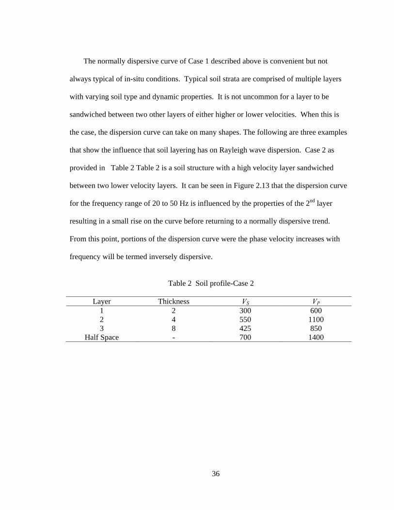
The normally dispersive curve of Case 1 described above is convenient but not
always typical of in-situ conditions. Typical soil strata are comprised of multiple layers
with varying soil type and dynamic properties. It is not uncommon for a layer to be
sandwiched between two other layers of either higher or lower velocities. When this is
the case, the dispersion curve can take on many shapes. The following are three examples
that show the influence that soil layering has on Rayleigh wave dispersion. Case 2 as
provided in Table 2 Table 2 is a soil structure with a high velocity layer sandwiched
between two lower velocity layers. It can be seen in Figure 2.13 that the dispersion curve
for the frequency range of 20 to 50 Hz is influenced by the properties of the 2nd layer
resulting in a small rise on the curve before returning to a normally dispersive trend.
From this point, portions of the dispersion curve were the phase velocity increases with
frequency will be termed inversely dispersive.
Table 2 Soil profile-Case 2
Layer Thickness VS VP
1 2 300 600 2 4 550 1100 3 8 425 850
Half Space - 700 1400

37
Figure 2.13 Dispersion curve for Case 2 soil profile with high velocity layer sandwiched between two lower velocity layers.
Case 3 is the inverse of Case 2 with a low velocity layer sandwiched between two
high velocity layers. The resulting dispersion curve reflects the low velocity layer as a
dip in the curve at 40 Hz and then is inversely dispersive up to 75 Hz where the curve
returns to a normal dispersive trend.
0 10 20 30 40 50 60 70 80 90 100250
300
350
400
450
500
550
600
650
Frequency (Hz)
Phas
e Ve
loci
ty V
R

38
Table 3 Soil profile-Case 3
Layer Thickness VS VP
1 2 425 850 2 4 300 600 3 8 550 1100
Half Space - 700 1400
Figure 2.14 Dispersion curve for Case 3 soil profile with low
velocity layer sandwiched between two higher velocity layers.
0 10 20 30 40 50 60 70 80 90 100300
350
400
450
500
550
600
650
Frequency (Hz)
Phas
e Ve
loci
ty V
R

39
The final example covers an important case where the dispersion curve is no longer
continuous. The soil profile of Case 4 in Table 4 is similar to that of Case 3 with the
exception that the low velocity layer has been further reduced in order achieve a
discontinuity in the dispersion curve. Figure 2.15 displays the resulting dispersion curve
and it can be seen that a jump occurs at approximately 90 Hz. Jumps in the dispersion
curve result when the medium properties within the zone of influence are no longer
governed by the fundamental mode of propagation (Lai and Rix, 1998). When a soil
profile contains either a high or low velocity layer sandwiched between two other layers,
higher Rayleigh modes can dominate the dispersion curve. The resulting curve requires a
mulit-mode analysis and inversion to be conducted in order for soil velocities to be
accurately determined.
Table 4 Soil profile-Case 4
Layer Thickness VS VP
1 2 425 850 2 4 220 440 3 8 550 1100
Half Space - 700 1400

40
Figure 2.15 Dispersion curve for Case 4 soil profile with low velocity layer sandwiched between two higher velocity layers resulting in a jump in the dispersion curve.
2.9 Rayleigh Wave Modes
As shown earlier in Section 2.6 the wavenumber k(ω) can be a multi-valued function
representing the total number of Rayleigh wave modes propagating within a specified
medium. These modes are solutions to Equation (2.6.6) that simultaneously satisfy the
free-surface boundary conditions and the decay of waves with depth. It has been shown
that higher mode Rayleigh waves can dominate the Rayleigh dispersion curve when
0 10 20 30 40 50 60 70 80 90 100200
250
300
350
400
450
500
550
600
650
Frequency (Hz)
Phas
e Ve
loci
ty V
R
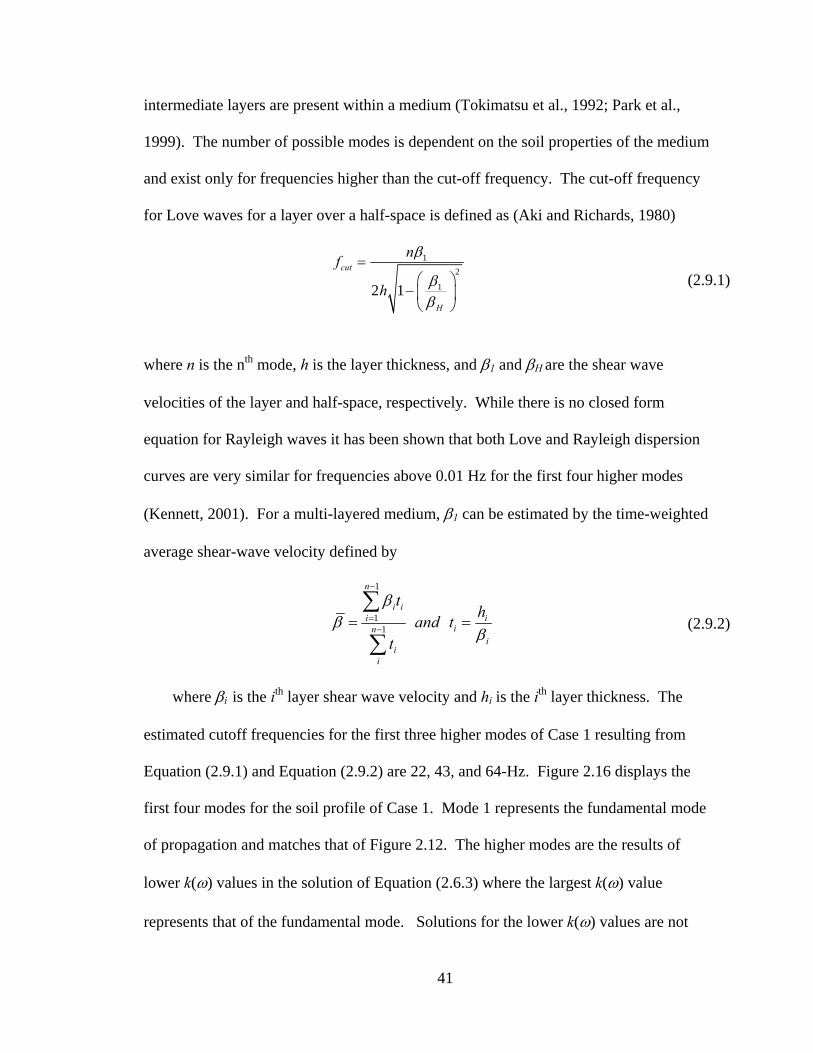
41
intermediate layers are present within a medium (Tokimatsu et al., 1992; Park et al.,
1999). The number of possible modes is dependent on the soil properties of the medium
and exist only for frequencies higher than the cut-off frequency. The cut-off frequency
for Love waves for a layer over a half-space is defined as (Aki and Richards, 1980)
1
2
12 1
cut
H
nf
h
β
ββ
=⎛ ⎞
− ⎜ ⎟⎝ ⎠
(2.9.1)
where n is the nth mode, h is the layer thickness, and β1 and βH are the shear wave
velocities of the layer and half-space, respectively. While there is no closed form
equation for Rayleigh waves it has been shown that both Love and Rayleigh dispersion
curves are very similar for frequencies above 0.01 Hz for the first four higher modes
(Kennett, 2001). For a multi-layered medium, β1 can be estimated by the time-weighted
average shear-wave velocity defined by
1
11
n
i ii i
ini
ii
thand t
t
ββ
β
−
=−= =
∑
∑ (2.9.2)
where βi is the ith layer shear wave velocity and hi is the ith layer thickness. The
estimated cutoff frequencies for the first three higher modes of Case 1 resulting from
Equation (2.9.1) and Equation (2.9.2) are 22, 43, and 64-Hz. Figure 2.16 displays the
first four modes for the soil profile of Case 1. Mode 1 represents the fundamental mode
of propagation and matches that of Figure 2.12. The higher modes are the results of
lower k(ω) values in the solution of Equation (2.6.3) where the largest k(ω) value
represents that of the fundamental mode. Solutions for the lower k(ω) values are not

42
possible below the cutoff frequency as seen in Figure 2.16.
Figure 2.16 Mutli-mode dispersion curves for Case 1. Modes 1 through 4 are represented by blue, green, red, and cyan open circles, respectively.
By definition, the wavenumber k is related to the wavelength λ in Equation (2.8.1) by
2kπλ =
(2.9.3)
As k changes so will λ resulting in longer wavelengths for smaller values of k. This
results in larger zones of penetration for modes with lower k values. Higher modes will
0 10 20 30 40 50 60 70 80 90 100250
300
350
400
450
500
550
600
650
700
750
Frequency (Hz)
Phas
e Ve
loci
ty V
R
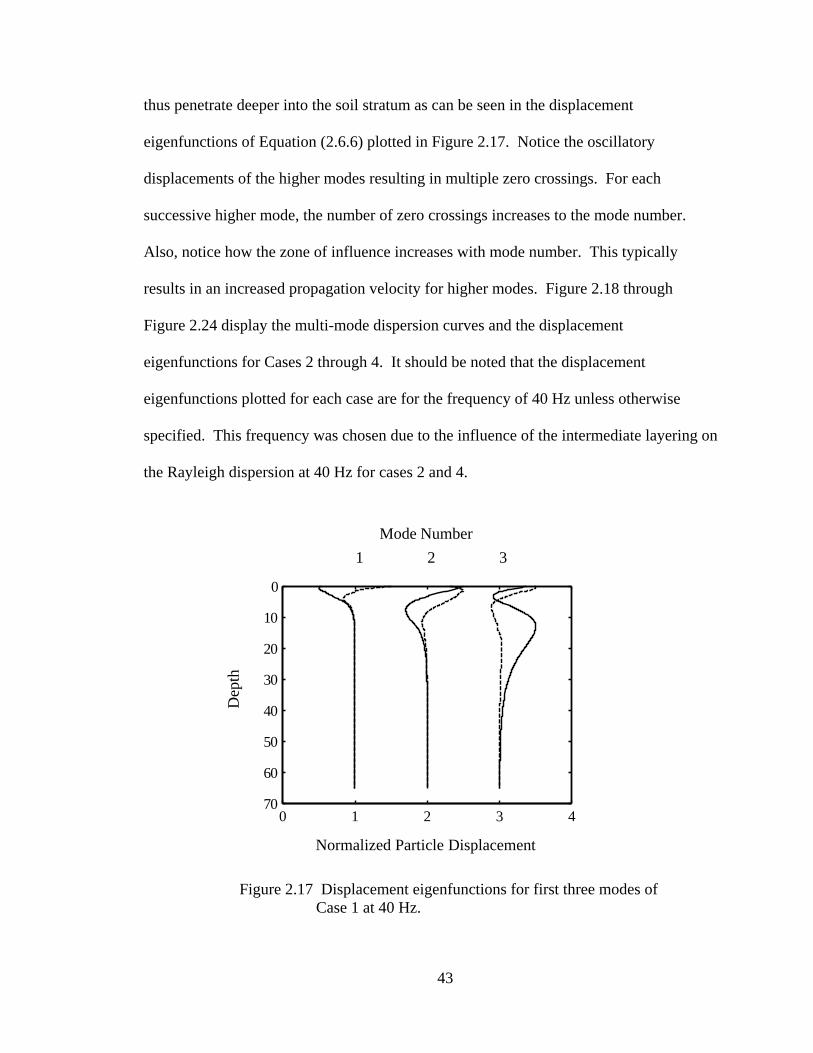
43
thus penetrate deeper into the soil stratum as can be seen in the displacement
eigenfunctions of Equation (2.6.6) plotted in Figure 2.17. Notice the oscillatory
displacements of the higher modes resulting in multiple zero crossings. For each
successive higher mode, the number of zero crossings increases to the mode number.
Also, notice how the zone of influence increases with mode number. This typically
results in an increased propagation velocity for higher modes. Figure 2.18 through
Figure 2.24 display the multi-mode dispersion curves and the displacement
eigenfunctions for Cases 2 through 4. It should be noted that the displacement
eigenfunctions plotted for each case are for the frequency of 40 Hz unless otherwise
specified. This frequency was chosen due to the influence of the intermediate layering on
the Rayleigh dispersion at 40 Hz for cases 2 and 4.
Figure 2.17 Displacement eigenfunctions for first three modes of Case 1 at 40 Hz.
Mode Number
Normalized Particle Displacement
1 2 3
Dep
th
0 1 2 3 4
0
10
20
30
40
50
60
70
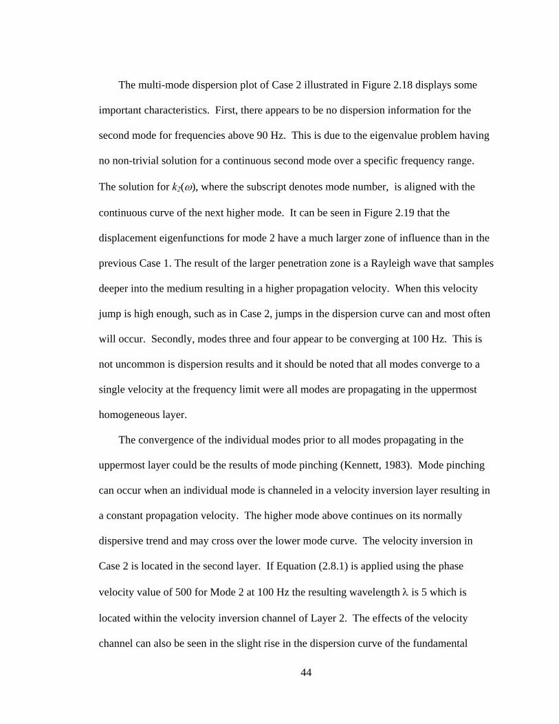
44
The multi-mode dispersion plot of Case 2 illustrated in Figure 2.18 displays some
important characteristics. First, there appears to be no dispersion information for the
second mode for frequencies above 90 Hz. This is due to the eigenvalue problem having
no non-trivial solution for a continuous second mode over a specific frequency range.
The solution for k2(ω), where the subscript denotes mode number, is aligned with the
continuous curve of the next higher mode. It can be seen in Figure 2.19 that the
displacement eigenfunctions for mode 2 have a much larger zone of influence than in the
previous Case 1. The result of the larger penetration zone is a Rayleigh wave that samples
deeper into the medium resulting in a higher propagation velocity. When this velocity
jump is high enough, such as in Case 2, jumps in the dispersion curve can and most often
will occur. Secondly, modes three and four appear to be converging at 100 Hz. This is
not uncommon is dispersion results and it should be noted that all modes converge to a
single velocity at the frequency limit were all modes are propagating in the uppermost
homogeneous layer.
The convergence of the individual modes prior to all modes propagating in the
uppermost layer could be the results of mode pinching (Kennett, 1983). Mode pinching
can occur when an individual mode is channeled in a velocity inversion layer resulting in
a constant propagation velocity. The higher mode above continues on its normally
dispersive trend and may cross over the lower mode curve. The velocity inversion in
Case 2 is located in the second layer. If Equation (2.8.1) is applied using the phase
velocity value of 500 for Mode 2 at 100 Hz the resulting wavelength λ is 5 which is
located within the velocity inversion channel of Layer 2. The effects of the velocity
channel can also be seen in the slight rise in the dispersion curve of the fundamental
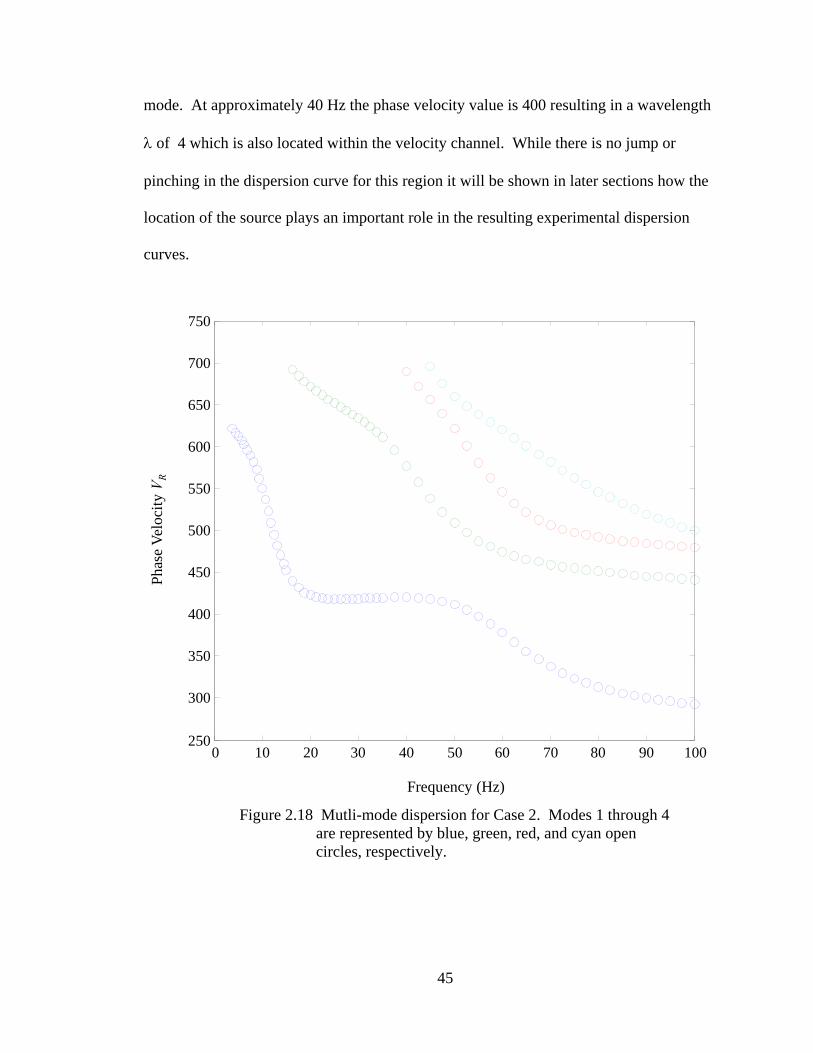
45
mode. At approximately 40 Hz the phase velocity value is 400 resulting in a wavelength
λ of 4 which is also located within the velocity channel. While there is no jump or
pinching in the dispersion curve for this region it will be shown in later sections how the
location of the source plays an important role in the resulting experimental dispersion
curves.
Figure 2.18 Mutli-mode dispersion for Case 2. Modes 1 through 4
are represented by blue, green, red, and cyan open circles, respectively.
0 10 20 30 40 50 60 70 80 90 100250
300
350
400
450
500
550
600
650
700
750
Frequency (Hz)
Phas
e Ve
loci
ty V
R

46
Figure 2.19 Displacement eigenfunctions for first three modes of Case 2 at 40 Hz.
The multi-mode dispersion plot of Case 3 in Figure 2.20 does not show any mode
jumps, but the first and second modes are close to converging at 85 Hz. At 40 Hz the
phase velocities for the first three modes are largely separated and the displacement
eigenfunctions of Figure 2.21 display large differences in their penetration depth. At 85-
Hz where Modes 1 and 2 come close to converging, the displacement eigenfunctions of
Figure 2.22 show similar penetration depths.
Figure 2.23 and Figure 2.24 display the multi-mode Rayleigh wave dispersion and
displacement eigenfuntions for Case 4. At 40 Hz, where the modes are greatly separated,
the resulting displacement eigenfunctions result in larger penetration depths at higher
modes. At 90 Hz where the jump in the dispersion is observed, the resulting
displacement eigenfunction for Mode 1 reflects a higher mode oscillating pattern with
0 1 2 3 4
0
20
40
60
80
Mode Number
Normalized Particle Displacement
1 2 3
Dep
th

47
multiple zero crossings (Figure 2.25). Notice the identical penetration depths for both
Modes 1 and 2.
Figure 2.20 Mutli-mode dispersion for Case 3. Modes 1 through 4 are represented by blue, green, red, and cyan open circles, respectively.
0 10 20 30 40 50 60 70 80 90 100250
300
350
400
450
500
550
600
650
700
750
Frequency (Hz)
Phas
e Ve
loci
ty V
R

48
Figure 2.21 Displacement eigenfunctions for first three modes of Case 3 at 40 Hz.
Figure 2.22 Displacement eigenfunctions for first three modes of Case 3 at 85 Hz.
0 1 2 3 4
0
10
20
30
40
50
60
Mode Number
Normalized Particle Displacement
1 2 3
Dep
th
Mode Number
Normalized Particle Displacement
1 2 3
Dep
th
0 1 2 3 4
0
5
10
15
20
25
30
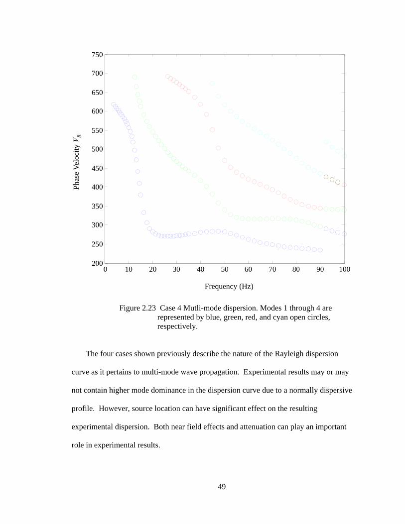
49
Figure 2.23 Case 4 Mutli-mode dispersion. Modes 1 through 4 are represented by blue, green, red, and cyan open circles, respectively.
The four cases shown previously describe the nature of the Rayleigh dispersion
curve as it pertains to multi-mode wave propagation. Experimental results may or may
not contain higher mode dominance in the dispersion curve due to a normally dispersive
profile. However, source location can have significant effect on the resulting
experimental dispersion. Both near field effects and attenuation can play an important
role in experimental results.
0 10 20 30 40 50 60 70 80 90 100200
250
300
350
400
450
500
550
600
650
700
750
Frequency (Hz)
Phas
e Ve
loci
ty V
R

50
Figure 2.24 Displacement eigenfunctions for first three modes of Case 4 at 40 Hz.
Figure 2.25 Displacement eigenfunctions for first three modes of Case 4 at mode jump.
Mode Number
Normalized Particle Displacement
1 2 3
Dep
th
0 1 2 3 4
0
10
20
30
40
50
Mode Number
Normalized Particle Displacement
1 2 3
Dep
th
0 1 2 3 4
0
5
10
15
20

51
2.10 Rayleigh Wave Attenuation
Attenuation, by definition, quantifies the amount of energy loss during propagation
of a seismic wave. There are two types of attenuation: intrinsic or material attenuation
caused by particle displacement resulting in energy dissipation as discussed in Section
2.1 and geometric attenuation, which is the loss of energy due to the spreading or
expansion of a seismic waves as they travel from a source.
Body and surface waves traveling along a free surface generated by a harmonic point
source differ in their geometric attenuation. Body waves attenuate at a rate proportional
to the distance r from the source as r-1 where surface waves attenuate at a rate of r-0.5
(Ewing et al., 1975). The lower attenuation rate of the surface waves compared to their
respective body waves makes surface waves ideal for site investigation requiring seismic
recording arrays of considerable length.
The above relationship for surface wave attenuation follows the principle of
conservation of energy and does not hold true for a non-homogeneous media (Lai and
Rix, 1998). Recalling the geometric spreading function ( , , )r zβ ωG from Section 2.6, Lai
and Rix showed that Rayleigh wave displacement fields are the result of the
superposition of multiple modes of propagation referred to as geometric dispersion.
Figure 2.26 displays the results for ( , , )r zβ ωG as a function of distance r from the source
for a homogeneous media and the four cases from Section 2.9 where z = 0 and ω = 40 Hz.
It is clear that for a heterogeneous media the geometric attenuation can be strongly
influenced by geometric dispersion resulting from media layering. Similar results for
geometric attenuation were also seen by Tokitmastu et al. (1992); Gucunski and Wood
(1991); and Lai and Rix (1998).
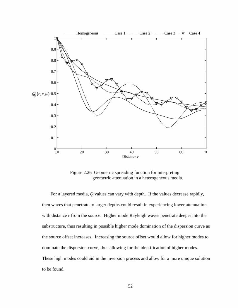
52
Figure 2.26 Geometric spreading function for interpreting geometric attenuation in a heterogeneous media.
For a layered media, Q values can vary with depth. If the values decrease rapidly,
then waves that penetrate to larger depths could result in experiencing lower attenuation
with distance r from the source. Higher mode Rayleigh waves penetrate deeper into the
substructure, thus resulting in possible higher mode domination of the dispersion curve as
the source offset increases. Increasing the source offset would allow for higher modes to
dominate the dispersion curve, thus allowing for the identification of higher modes.
These high modes could aid in the inversion process and allow for a more unique solution
to be found.
10 20 30 40 50 60 700
0.1
0.2
0.3
0.4
0.5
0.6
0.7
0.8
0.9
1
Homogeneous Case 1 Case 2 Case 3 Case 4
Distance r
( , , )r zβ ωG

53
2.11 Inversion
Inversion is the process of determining either an unknown input to a system or a set of
unknown system characteristics coupled to a system response. For the Rayleigh inverse
problem it is the system characteristics GB(z), GS(z), and ρ(z) that are unknown. The system
input is defined by the harmonic source and the system response by the Raleigh wave
dispersion curve.
Inverse problems often suffer from instability since they are not well-posed. Jacques
Hadamard, a French mathematician, defined a well-posed problem as one that models
physical phenomena with the following properties
a. A solution exists
b. The solution is unique
c. The solution depends continuously on the data
For the Rayleigh inverse problem, it is property “b” that is most often violated due to
either lack of sufficient information or problem constraints. Many solutions can exist for a
given dispersion that meets the minimum criteria for a solution. Additional information such
as material properties and layer geometry obtained from soil logs can help to reach a global
solution; however, this defeats the purpose of non-invasive techniques. This research
minimizes the problem of multiple solutions by mapping the higher modes of propagation
over a range of frequencies for inversion. The higher modal velocities provide the necessary
additional information for inversion to possibly achieve a unique solution.
The inversion of Rayleigh wave dispersion has been studied for over 50 years
(Thompson, 1950; Haskell, 1953; Nazarian, 1984; Horike, 1985; Tokimatsu, 1995; Lai and
Rix, 1998; Park et al., 1999; Zywicki, 1999; Hebeler, 2001; and Zarrabi 2005). While each

54
study has provided different methods for approaching the inverse problem, they all can be
viewed as either local or global search procedures.
Local searches initially guess a solution to a functional and then refine the solution
until convergence to a stationary point is achieved. An inherent limitation to local
techniques is that the functional must be smooth and that its derivatives both exist and are
continuous. It is also necessary that the initial guess be sufficiently close to the solution in
order to achieve convergence and then there is still no guarantee that a global solution has
been found.
Global searches take advantage of the entire solution space in order to achieve
convergence to a global solution. They are not constrained by initial guesses and do rely on
gradient-based methods. However they can require significantly more time to arrive at a
solution and thus are more expensive.
For this research the global search technique genetic algorithm (GA) is used based on
the research by Zarrabi (2005). The genetic algorithm is a search technique that utilizes the
mechanics of natural selection and genetics. The overall goal of the GA is to minimize an
objective function that represents the error between the theoretical and experimental Rayleigh
dispersion curves.
In genetic algorithms parlance, generations are the iterative steps used in determining
solutions to the objective function and selecting solutions based on their performance or
fitness. The variables associated with the selected solutions are transformed into binary
strings where crossover can occur. Crossover recombines the binary coding of selected
variables to produce an offspring to be used as a solution along with the original variables in
the next generation.
Mutation is the random alteration of an encoded variable and is performed so that the
probability of searching a particular subspace is never zero. The process continues until a
55
maximum number of generations is achieved or some minimum criterion for the objective
function is met.
The Rayleigh dispersion equation used in the objective function contains multiple
variables that result in an extremely large search space. Rix et al. (1991) showed that the
influences of the Poisson’s ratio and mass density on the Rayleigh dispersion equation are of
secondary importance. The parameters seldom change from their initial values and can be
considered constants; therefore, Equation (2.6.8) can be re-written as
[ ], 0R s =H VF (2.11.1)
where H is a vector representing the layer thicknesses and Vs is the vector representing the
layer shear-wave velocities. Equation (2.11.1) reduces the Rayleigh dispersion equation to
only two variable sets thus largely reducing the overall search space.
The forward solution to Equation (2.11.1) is achieved through computer code
developed by Rix and Lai (1999) based on the research methods of Lai and Rix (1998) and
Hisada (1994) from Section 2.6. For each generation of the GA, the objective function
calculates the error between the forward solution of Equation (2.11.1) and the experimental
Rayleigh dispersion by
exp theoR Rerror = −V V (2.11.2)
where expRV are the Rayleigh wave phase velocities obtained from experimental results, theo
RV
are the theoretical Rayleigh wave phase velocities from Equation (2.11.1), and is the
Euclidian norm. The GA is halted when a minimum of Equation (2.11.2) is met or when a
maximum number of pre-set generations is achieved.

56
The only alteration to the genetic algorithm from Zarrabi (2005) is the adjustment for
multiple mode dispersion. Equation (2.11.2) is evaluated in the same manner; however, the
theoretical Rayleigh wave velocities used are a composite of individual modal phase
velocities over their respective frequency ranges. Each mode is weighted equally so as to not
influence the results for a particular mode.
Rayleigh wave propagation is a complex problem involving combinations of
multiple-modes of propagation. In order for inversion to be accurate, correct
identification of higher-mode Rayleigh wave propagation is essential. The following
section will show the typical methods used for both the passive and active source
measurements of Rayleigh wave propagation for the determination of Rayleigh phase
velocity.

57
Chapter 3. Rayleigh Surface Wave Measurements
The theoretical relationships of Chapter 2 result in Rayleigh wave dispersion
calculations based on given soil parameters. However, as is often the case, it is the soil
parameters themselves that are unknown. Therefore, if the dispersion relating to the soil
conditions is known, then the parameters can be determined through an inversion process.
Surface wave techniques for the measurement of Rayleigh wave dispersion have
been researched for over 30 years. They have evolved from simple two-sensor methods
(Stoke et al., 1994) into vast multi-sensor arrays (Park et al., 1999). This chapter
describes in detail the different methods used for the determination of Rayleigh wave
dispersion using both active and passive source techniques.
3.1 Spectral Analysis of Surface Waves
The spectral analysis of surface waves (SASW) is a non-invasive method used for
the determination of low-strain in-situ soil conditions. The SASW method measures the
phase angles for the propagating surface plane waves at various points along an array of
receivers. These phase angles are then used to determine frequency-dependent phase
velocities. These frequency-dependent phase velocity measurements are the Rayleigh
wave dispersion discussed in Section 2.8.
Traditional SASW testing (Nazarian 1984; Nazarian and Stoke; 1984; and Stoke
1994) uses two receivers and a source, typically a sledge hammer or weight drop device.
The receivers are placed a certain distance apart, the source is activated, and the resulting
surface waves are recorded. Heisey (1982) suggested that the receiver spacing should be
greater than one-third and less than two wavelengths. However, as layer velocities are
unknown and the resulting wavelength can vary greatly as seen in Section 2.8, testing

58
with various receiver spacings results in more reliable measurements (Stoke 1994).
Stoke (1994) suggested a more appropriate relationship between receiver spacing and
wavelength to be one-half to three times the wavelength.
Two common testing procedures are used with the two receiver spacing technique
described above: common source/receiver (CSR) and common midpoint geometry
(CMP) . In the CSR method either the source or receivers are fixed in place while the
other is moved during testing (Figure 3.1 top). In the CMP method both the receivers and
the source are moved an equal distance about an imaginary centerline (Figure 3.1
bottom). Theoretically both methods should produce the same results if the medium is
horizontally homogeneous.
A spectrum analyzer is used to determine the phase difference recorded between
receivers. By using the principle of a rotating vector, the travel time between two
receivers can be determined by (Stoke 1994)
2 2Δ T Δt
fφ φπ π
= = (3.1.1)
where Δφ is the phase difference, T is the period, and f is the frequency of propagation. If
Δx is the distance between the two receivers, then the phase velocity can be determined
by
RxV
tΔ
= (3.1.2)

59
The term VR represents the Rayleigh wave phase velocity, which will be used throughout
the rest of this paper instead of surface wave velocity since Rayleigh waves are the focus
of the research.
Figure 3.1 CSR (top) and CMP (bottom) testing procedures. (Adopted from Rix 2000).
CL
Sensor
Source

60
One limitation of the SASW method is an inability to recognize multiple mode wave
propagation. The phase difference between the two receivers is assumed linear but, as
Section 2.6 points out, the propagating wave can be a superposition of multiple mode
waves resulting in an effective propagating phase velocity that may not be linear.
3.2 Multi-Channel Analysis of Surface Waves
The multi-channel analysis of surface waves (MASW) method utilizes an array of
receivers to determine phase change without having to move receivers. The length and
geometry of the array is dependent on the desired wavenumber k(ω) resolution and will
be discussed in more detail in Chapter 5. Two types of arrays are generally used:
uniform and non-uniform (Figure 3.2). Information gathered from uniform arrays limits
uncertainties in the processing of data where as non-uniform arrays allow for information
to be gathered over distances with fewer receivers. Later sections will show in more
detail how non-uniform arrays produce results that can lead to errors if the signal
processing theory is not well understood.
Figure 3.2 MASW array setup for uniform (top) and non-uniform (bottom) sensor spacing.
Sensor
Source

61
3.3 Regression Line Slope Method
The regression line slope method (RLS) for MASW uses the cross power method to
determine the phase difference between receivers (Zarrabi, 2005). The cross power
method first estimates the power spectral densities of each receiver along the array using
the discrete Fourier transform (DFT)
( )1
0( ) ( )exp
N
i i n nn
S s t j tω ω−
=
= −∑ (3.3.1)
where Si(ω) is the complex-valued power spectrum of the receiver located in the ith
position of the receiver array, ω is the circular frequency (equal to 2π f where f is the
propagating frequency), j is an imaginary number, and N is the total number of samples
recorded by the receiver. The cross power is then determined by array multiplying the
power spectrum of one receiver and the complex conjugate of the power spectrum of the
other receiver:
*( ) ( ) ( )
m nS S n mY S Sω ω ω= ⋅ (3.3.2)
where * denotes complex conjugate. The complex conjugate is applied so the phase
change between the two receivers is accounted for in the resulting complex value which
can then be determined from the following relationship
{ }{ }
1( )
( ) tan( )
m n
m n
S Smn
S S
Y
Y
ωφ ω
ω−
⎡ ⎤ℑ⎢ ⎥=⎢ ⎥ℜ⎣ ⎦
(3.3.3)
62
where ℑandℜ are the imaginary and real parts of the complex valued ( )m nS SY ω . This
process is repeated for each receiver in the array with respects to reference receiver m. If
the signal being recorded is a propagating monochromatic plane wave then the resulting
phase difference as a function of distance should result in a linear relationship whose
slope represents the wavenumber k(ω). Recalling from Section 2.3 that
2 f tkx
π ΔΔ
= (3.3.4)
and that the travel time from Section 3.1 is
2
Δtf
φπ
= (3.3.5)
the following relationship can be derived:
2
tx x f
ΔφΔ Δ πΔ
= (3.3.6)
From this it can be deduced that the slope is
kx
ΔφΔ
=
(3.3.7)
The resulting phase changes are plotted in (Figure 3.3) with respect to the distance
between the reference receiver m and all other individual receivers. It is apparent that the
initial phase differences (open circles) do not represent a constant slope. Recognizing
that Equation (3.3.7) is a function of the period T which is related to the wavelength λ as

63
RV fTλλ= =
(3.3.8)
if the array length is longer than the propagating wavelength λ then the corresponding
phase information recorded from the array, past the length of λ, will need to be
unwrapped by 2π. This can be conceptualized by the rotating vector completing one full
2π rotation where the phase begins to repeat itself. By applying a 2π unwrap to the phase
angles at jumps of π or greater, a constant slope can be achieved. This slope represents
the wavenumber k(ω) of propagation (solid circles).
Figure 3.3 Phase difference as a function of distance (open circles) and unwrapped phase angles (solid circles).
However, if the signal is a superposition of multiple modes, the unwrapping process
may result in the phase angles oscillating around a dominant mode of propagation
(Zywicki, 1999). Figure 3.4 displays the results of the RLS method when a signal
-15-13-11-9-7-5-3-113
0 20 40 60
2π4π
Δx
Δφ
λ
Phas
e Ang
le (r
ad)
Distance x From Source
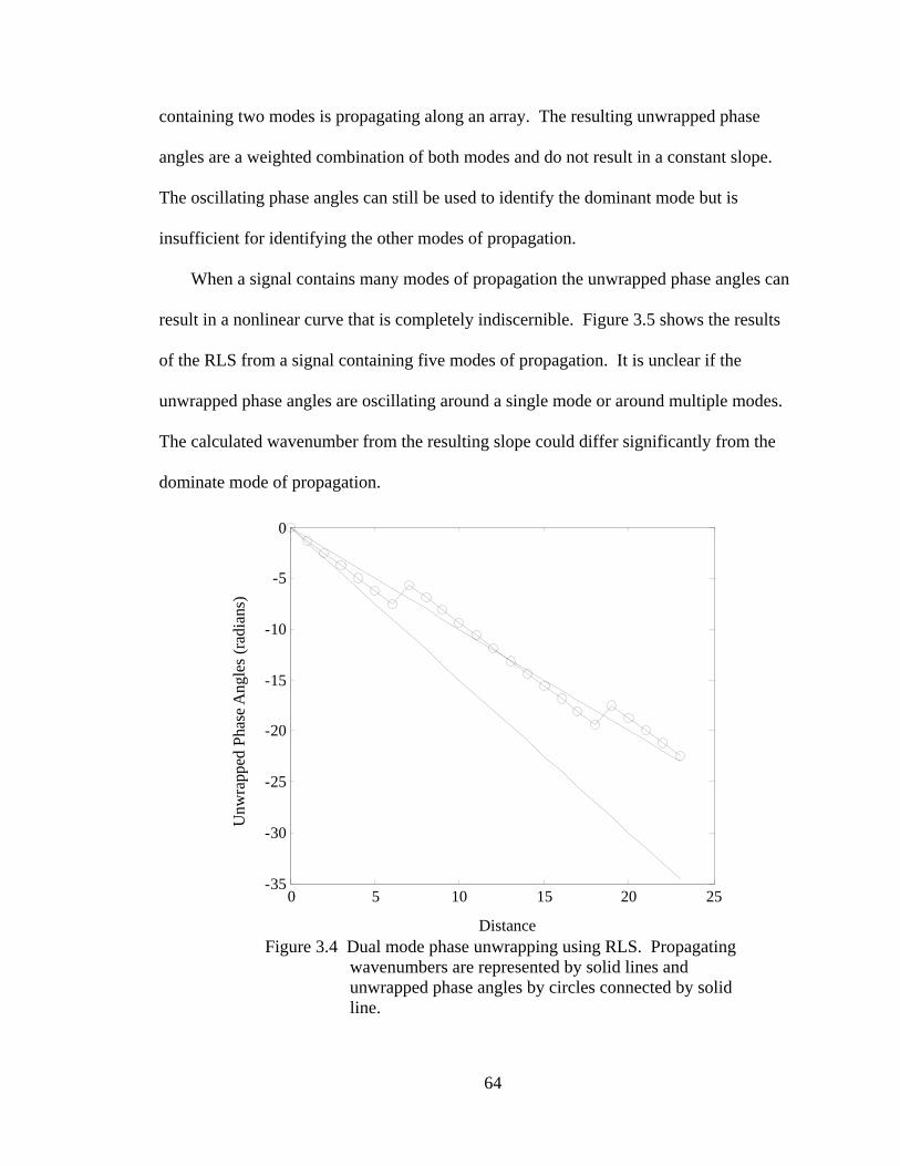
64
containing two modes is propagating along an array. The resulting unwrapped phase
angles are a weighted combination of both modes and do not result in a constant slope.
The oscillating phase angles can still be used to identify the dominant mode but is
insufficient for identifying the other modes of propagation.
When a signal contains many modes of propagation the unwrapped phase angles can
result in a nonlinear curve that is completely indiscernible. Figure 3.5 shows the results
of the RLS from a signal containing five modes of propagation. It is unclear if the
unwrapped phase angles are oscillating around a single mode or around multiple modes.
The calculated wavenumber from the resulting slope could differ significantly from the
dominate mode of propagation.
Figure 3.4 Dual mode phase unwrapping using RLS. Propagating
wavenumbers are represented by solid lines and unwrapped phase angles by circles connected by solid line.
0 5 10 15 20 25-35
-30
-25
-20
-15
-10
-5
0
Distance
Unw
rapp
ed P
hase
Ang
les (
radi
ans)

65
Figure 3.5 Multi mode phase unwrapping using RLS. Propagating wavenumbers are represented by solid lines and unwrapped phase angles by circles connected by solid line.
3.4 Frequency Wavenumber Method
The frequency-wavenumber (f-k) method has been used by several researchers
including Zywicki (1999), Foti (2000), Hebeler (2001), and Rix et al. (2001). The f-k
method is based on the technique known as beamforming as outlined in Johnson and
Dudgeon (1993). Beamforming is a type of spatial filtering that focuses an array’s signal
capturing abilities in a particular direction through the use of a steering vector. The
output of the f-k method is a steered response power with peaks in the power spectrum
representing the wavenumbers of the propagating plane waves and is defined by
0 5 10 15 20 25-35
-30
-25
-20
-15
-10
-5
0
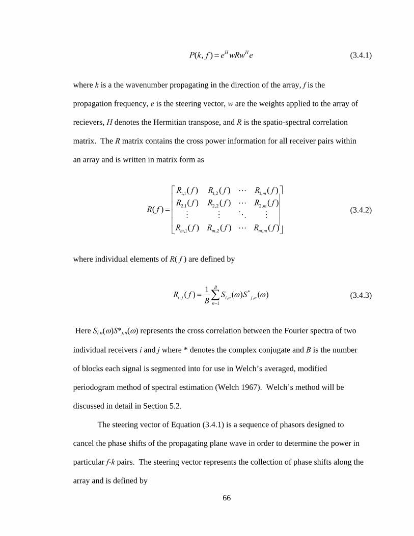
66
( , ) H HP k f e wRw e= (3.4.1)
where k is a the wavenumber propagating in the direction of the array, f is the
propagation frequency, e is the steering vector, w are the weights applied to the array of
recievers, H denotes the Hermitian transpose, and R is the spatio-spectral correlation
matrix. The R matrix contains the cross power information for all receiver pairs within
an array and is written in matrix form as
1,1 1,2 1,
2,1 2,2 2,
,1 ,2 ,
( ) ( ) ( )( ) ( ) ( )
( )
( ) ( ) ( )
m
m
m m m m
R f R f R fR f R f R f
R f
R f R f R f
⎡ ⎤⎢ ⎥⎢ ⎥=⎢ ⎥⎢ ⎥⎣ ⎦
(3.4.2)
where individual elements of R( f ) are defined by
*, , ,
1
1( ) ( ) ( )B
i j i n j nn
R f S SB
ω ω=
= ∑ (3.4.3)
Here Si,n(ω)S*j,n(ω) represents the cross correlation between the Fourier spectra of two
individual receivers i and j where * denotes the complex conjugate and B is the number
of blocks each signal is segmented into for use in Welch’s averaged, modified
periodogram method of spectral estimation (Welch 1967). Welch’s method will be
discussed in detail in Section 5.2.
The steering vector of Equation (3.4.1) is a sequence of phasors designed to
cancel the phase shifts of the propagating plane wave in order to determine the power in
particular f-k pairs. The steering vector represents the collection of phase shifts along the
array and is defined by

67
1
2
exp( )exp( )
( )
exp( )m
jkxjkx
e k
jkx
−⎡ ⎤⎢ ⎥−⎢ ⎥=⎢ ⎥⎢ ⎥−⎣ ⎦
(3.4.4)
where e is the phase shift vector associated with trial wavenumber k in the direction of
the receiver array and x1, x2, .. xm are the receiver locations in the array.
Shading can be applied through the use of a diagonal weighting matrix. Shading
can enhance the beamformer’s shape and reduce side lobe heights, resulting in better
frequency-wavenumber resolution. The weighting matrix is the collection of receiver
weights placed along the diagonal defined as
1 2( ) mw x diag x x x⎡ ⎤= ⎣ ⎦ (3.4.5)
Figure 3.6 displays a steered response for a Raleigh plane wave propagating with a
velocity of 305 ft/sec and a corresponding k value of 0.7854. The steered response
results in a wavenumber spectrum with the maximum energy located at the propagating
wavenumber.

68
Figure 3.6 Steered response of a plane wave propagating with wavenumber k = 0.7854.
3.5 Refreaction Microtremor
The Refraction Microtremor (ReMi) method, as described in Louie (2001), is used in
the determination of Rayleigh wave phase velocity determined from ambient noise and is
based on the p-τ transformation or slantstack (Thorson and Claerbout, 1985), The p-τ
transformation is defined as
( , ) ( , )x
A p A x t px dxτ τ= = +∫ (3.5.1)
where x is distance, t is time, τ is the intercept time, and p is the slope of the line
representing dt/dx, the inverse of apparent velocity in the direction of x. Equation (3.5.1)
maps a two dimensional sequence in space-time into another two dimensional sequence
in slowness-intercept time. In its discrete form Equation (3.5.1) is defined as
1
0
( , ) ( , )nx
oj
A p p ldp kdt A x jdx t idt pxτ τ−
=
= + = = = = = +∑
(3.5.2)
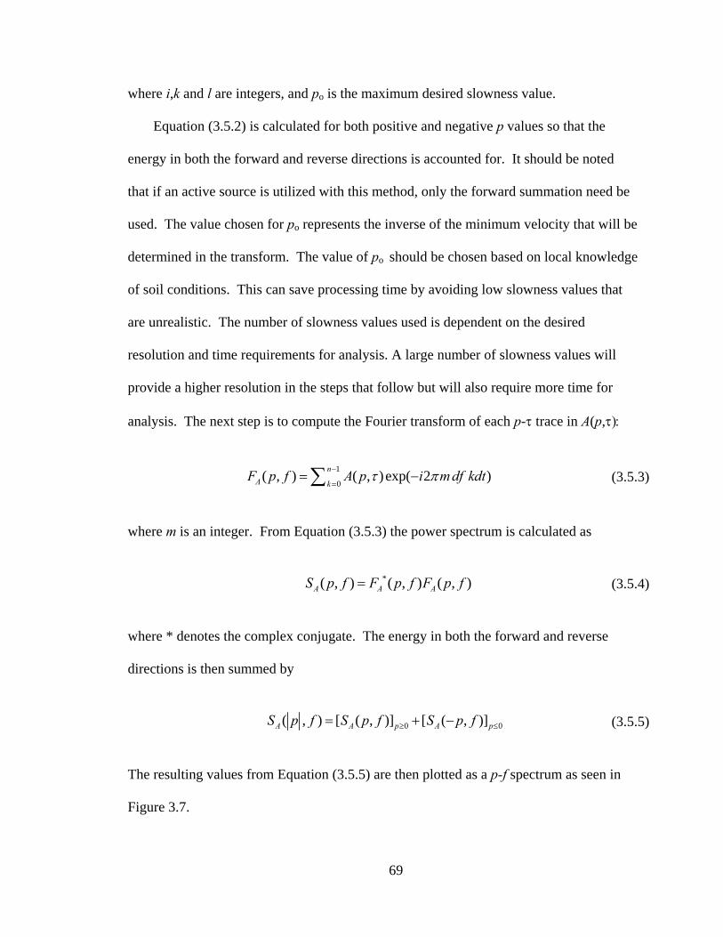
69
where i,k and l are integers, and po is the maximum desired slowness value.
Equation (3.5.2) is calculated for both positive and negative p values so that the
energy in both the forward and reverse directions is accounted for. It should be noted
that if an active source is utilized with this method, only the forward summation need be
used. The value chosen for po represents the inverse of the minimum velocity that will be
determined in the transform. The value of po should be chosen based on local knowledge
of soil conditions. This can save processing time by avoiding low slowness values that
are unrealistic. The number of slowness values used is dependent on the desired
resolution and time requirements for analysis. A large number of slowness values will
provide a higher resolution in the steps that follow but will also require more time for
analysis. The next step is to compute the Fourier transform of each p-τ trace in A(p,τ):
1
0( , ) ( , ) exp( 2 )n
A kF p f A p i m df kdtτ π−
== −∑ (3.5.3)
where m is an integer. From Equation (3.5.3) the power spectrum is calculated as
*( , ) ( , ) ( , )A A AS p f F p f F p f= (3.5.4)
where * denotes the complex conjugate. The energy in both the forward and reverse
directions is then summed by
0 0( , ) [ ( , )] [ ( , )]A A p A pS p f S p f S p f≥ ≤= + − (3.5.5)
The resulting values from Equation (3.5.5) are then plotted as a p-f spectrum as seen in
Figure 3.7.

70
The energy spectrum of Figure 3.7 displays the energy distribution for propagating
waves along the line of receivers in x as a function of slowness vs. frequency. The
squares plotted along the area of the spectrum where light green areas meets the dark blue
areas are considered the energy of the surface waves propagating most directly along the
line of receivers in x. The reason for this is that any surface wave contributing to the
energy spectrum propagating at angles oblique to the line of receivers in x will result in
lower slowness or higher apparent phase velocities. This raises an interesting question as
to what happens if there is no energy directly along the line. The chosen velocities would
then be overestimated by some amount. This can be overcome by creating a source at the
end of the line to ensure propagation along the line.
Figure 3.7 p-f spectrum obtained from ReMi method using 24 receivers spaced 8 meters apart.
Slow
ness
(sec
/m)
Frequency (Hz)
0.0 20.0
0.002

71
The energy band in the direction opposite to the normal dispersion is due to spatial
aliasing. Just as temporal sampled data results in a Nyquist frequency (see Section 5.1)
defining aliasing criteria, spatially sampled data results in a spatial Nyquist frequency due
to slowness wraparound. Care must be taken in choosing velocity values to the right of
the aliasing band due to possible spectral leakage. For this research velocities will not be
chosen beyond the spatial aliasing bands. The velocity information beyond the bands
will be supplied via the MASW method.
3.6 Source Methods
The Rayleigh waves recorded for the before-mentioned surface wave techniques
come from either passive or active sources. Passive sources are ideal due to the fact they
require less equipment and less physical effort. However, it should be understood that
the energy formed by the passive source comes from an active source somewhere in or on
the earth. The sources can be mini earthquakes, vehicle traffic, ocean tides, or any other
action that imparts force into or on the earth. Therefore, by labeling a source as either
active or passive is simply stating whether or not the recorded waves were generated by
the person or persons conducting the experiment.
Active sources are typically viewed as either an impulse or harmonic source. An
impulse source can be a sledge hammer, weight drop mechanism, or any other
mechanism that applies a dynamic point force of energy into the earth. Advantages of
point sources include multiple frequency generation with each application and trigger
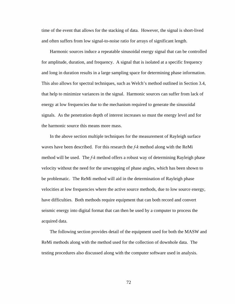
72
time of the event that allows for the stacking of data. However, the signal is short-lived
and often suffers from low signal-to-noise ratio for arrays of significant length.
Harmonic sources induce a repeatable sinusoidal energy signal that can be controlled
for amplitude, duration, and frequency. A signal that is isolated at a specific frequency
and long in duration results in a large sampling space for determining phase information.
This also allows for spectral techniques, such as Welch’s method outlined in Section 3.4,
that help to minimize variances in the signal. Harmonic sources can suffer from lack of
energy at low frequencies due to the mechanism required to generate the sinusoidal
signals. As the penetration depth of interest increases so must the energy level and for
the harmonic source this means more mass.
In the above section multiple techniques for the measurement of Rayleigh surface
waves have been described. For this research the f-k method along with the ReMi
method will be used. The f-k method offers a robust way of determining Rayleigh phase
velocity without the need for the unwrapping of phase angles, which has been shown to
be problematic. The ReMi method will aid in the determination of Rayleigh phase
velocities at low frequencies where the active source methods, due to low source energy,
have difficulties. Both methods require equipment that can both record and convert
seismic energy into digital format that can then be used by a computer to process the
acquired data.
The following section provides detail of the equipment used for both the MASW and
ReMi methods along with the method used for the collection of downhole data. The
testing procedures also discussed along with the computer software used in analysis.

73
Chapter 4. Testing and Equipment
The techniques described in Chapter 3 require that surface wave measurements be
collected for processing. Depending on the frequency range of interest, one technique
may offer more reliable measurements than another. The MASW methods offers good
signal-to-noise ratio for high frequencies but suffer at frequencies below 10 Hz (Hebeler,
2001). The ReMi method can fill this gap by using low frequency noise in its dispersion
calculations (Louie, 2001). For this research each site contained a borehole that was used
to find the in-situ shear-wave velocities and was used as a control test for the two non-
invasive methods. The following sections describe the testing procedures and equipment
used in both the invasive and non-invasive methods along with the collection of
downhole data.
4.1 MASW Testing and Equipment
In order to take advantage of the signal-to-noise ratio and sampling size offered by a
harmonic source, surface waves were generated using the APS Model 400 Electro-SEIS
Shaker (Figure 4.1). The Shaker has a weight of 160 lbs. and is capable of applying a
force (sine peak) up to 100 lb as shown in the force envelope plot of Figure 4.2. The
APS system can be used to generate either a single or a swept sine wave for frequencies
up to 200 Hz. The model is rated to 15 amperes, which is supplied by the APS Model
144 Dual-Mode Amplifier (Figure 4.3). The amplifier has a current output of 15 amperes
and a frequency range of 0 to 2000 Hz.

74
Figure 4.1 APS Model 400 ELECTRO-SEIS Shaker.
Figure 4.2 Force envelope for Model 400 Shaker.
Frequency Hz
Forc
e –
LB
1.0 10 10010
100
Free BodyZero Velocity Load
Free Body Maximum Power Into Load
Fixed Body Amplifier Limit

75
Figure 4.3 APS Model 144 Dual-Mode Amplifier.
Sinusoidal waves are generated using the Hewlett Packard 33120A
Function/Arbitrary Waveform Function Generator distributed by Agilent Technologies
(Figure 4.4). The 33120A can produce individual and swept sinusoidal waveforms
ranging from 100μHz to 15 MHz and is controlled via USB interface using the computer
software VEE Pro.
Figure 4.4 Hewlett Packard 33120A Function/Arbitrary Waveform Function Generator.

76
VEE Pro is a graphical language environment with built-in auto-detect functionality
for using Agilent instruments. The graphical user interface is user friendly and the
program contains a large library of signal processing tools. A program called
“SASW_Testing” was developed using VEE Pro to generate sinusoidal signals for a
range of frequencies over specified time periods. For this research each frequency was
generated for ten seconds. This duration was chosen so that a specific number of
windows could be applied using Welch’s method from Section 3.4. The program begins
by establishing all communication with the external devices (Figure 4.5). Once this is
accomplished, the program sends the waveform information to the waveform generator,
which then generates the signal and transmits the waveform to the 144 dual-mode
amplifier. The signal is then amplified and passed to the Shaker where harmonic
excitation commences.
As the Rayleigh waves generated by the shaker propagate they are recorded by an
array of 15 Wilcox 731A seismic accelerometers. The accelerometers are shown in
Figure 4.6 along with the metal base fabricated in-house to secure the sensors in the
ground. Each accelerometer is powered by the Wilcox P31 Power Unit/Amplifier
(Figure 4.7). The P31 is a ultra-low-noise power unit and amplifier with optional gain
and filter settings.
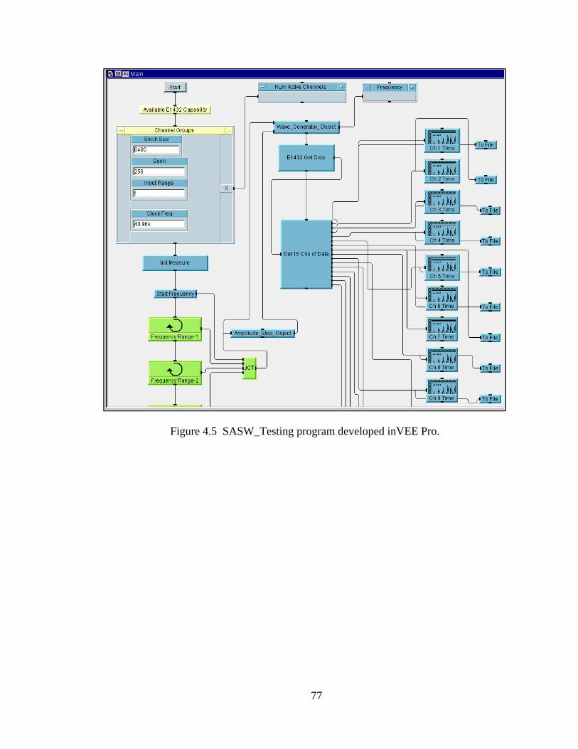
77
Figure 4.5 SASW_Testing program developed inVEE Pro.
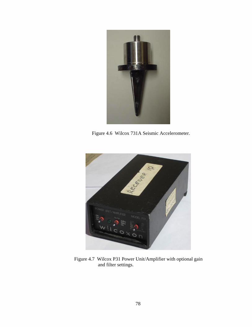
78
Figure 4.6 Wilcox 731A Seismic Accelerometer.
Figure 4.7 Wilcox P31 Power Unit/Amplifier with optional gain and filter settings.

79
The signals received by the accelerometers are recorded using the VT1432A 16-
channel 24-bit digitizer by VXI Technologies. It has a maximum sampling rate of 51,200
samples/sec. The VT1432A is controlled by the CT-100C portable VXIbus mainframe,
which is connected to a computer via USB port. The SASW_Testing program discussed
above simultaneously controls the CT-100C along with the waveform generator. The
VEE program was set up to pass the recorded information from the CT-100C for each
accelerometer to an individual ASCII file (Figure 4.5) and to display the current signal in
the display panel for viewing during testing (Figure 4.9). The main display panel
contains a waveform plot for each receiver in the array that allows for the signal to be
viewed during testing. A small display panel in the bottom right of the panel displays the
current frequency of excitation. Figure 4.10 shows a zoomed in view of a waveform plot
during testing. A typical setup of the data acquisition equipment is shown in Figure 4.11.
Figure 4.8 CT-100C portable VXIbus mainframe with slotted VT1432A 16-channel 24-bit digitizer.

80
Figure 4.9 Main Panel of SASW_Testing program.
Figure 4.10 Zoomed in view of a waveform plot for a 35-Hz signal.

81
Figure 4.11 Data acquisition Equipment. From left to right: Computer with VEE Pro software; 33120A Function/Arbitrary Waveform Function Generator; CT-100C portable VXIbus mainframe with slotted VT1432A 16-channel 24-bit digitizer; and 144 Dual-Mode Amplifier.
4.2 ReMi Testing and Equipment
The recording of surface waves for the ReMi method was accomplished using 24
4.5-Hz geophones (Figure 4.12). Geophones were used because the data acquisition
equipment with the ReMi method has a specific connection and cables designed for use
with geophones. However, geophones would still be the preferred choice due to the large
amount of wire that would be required for the accelerometers. The data was acquired
using the DAQLink II, 24-bit, 24-channel data acquisition box manufactured by
SeismicSources (Figure 4.13). Powered by a portable 12-volt battery, the DAQLink II is
small and extremely light (3 lbs) with a power consumption of less than 0.4 Watts per
channel, making it ideal for field testing. It has internal storage of up to 2GB of data and
standard output formats include SEG-Y, SEG-2, and ASCII. The DAQLink II can record
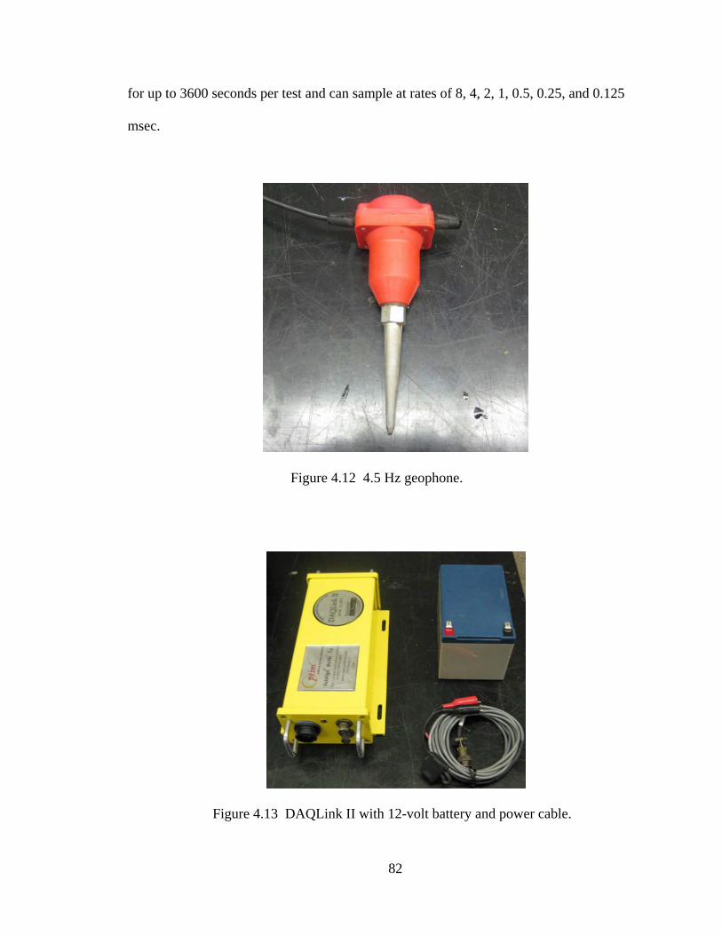
82
for up to 3600 seconds per test and can sample at rates of 8, 4, 2, 1, 0.5, 0.25, and 0.125
msec.
Figure 4.12 4.5 Hz geophone.
Figure 4.13 DAQLink II with 12-volt battery and power cable.

83
The collection of the seismic traces was handled using the computer software
program Vibrascope produced by Seismic Source. Vibrascope is a seismic data
acquisition system that allows the collection, viewing, and analysis of seismic traces.
Figure 4.14 displays the trace viewing screen incorporated into the Vibrascope program.
From this screen you can also choose to view the spectrum, seismic correlation, and noise
statistics of any or all of the traces. For this research the program was only used to record
the seismic traces. All other signal processing was conducted using the computer
program SeisOpt ReMi.
Figure 4.14 Vibrascope program displaying recorded traces.
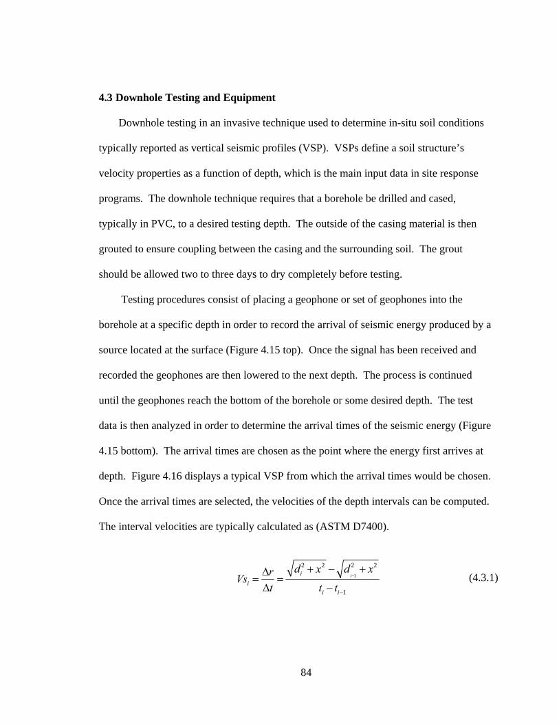
84
4.3 Downhole Testing and Equipment
Downhole testing in an invasive technique used to determine in-situ soil conditions
typically reported as vertical seismic profiles (VSP). VSPs define a soil structure’s
velocity properties as a function of depth, which is the main input data in site response
programs. The downhole technique requires that a borehole be drilled and cased,
typically in PVC, to a desired testing depth. The outside of the casing material is then
grouted to ensure coupling between the casing and the surrounding soil. The grout
should be allowed two to three days to dry completely before testing.
Testing procedures consist of placing a geophone or set of geophones into the
borehole at a specific depth in order to record the arrival of seismic energy produced by a
source located at the surface (Figure 4.15 top). Once the signal has been received and
recorded the geophones are then lowered to the next depth. The process is continued
until the geophones reach the bottom of the borehole or some desired depth. The test
data is then analyzed in order to determine the arrival times of the seismic energy (Figure
4.15 bottom). The arrival times are chosen as the point where the energy first arrives at
depth. Figure 4.16 displays a typical VSP from which the arrival times would be chosen.
Once the arrival times are selected, the velocities of the depth intervals can be computed.
The interval velocities are typically calculated as (ASTM D7400).
1
2 2 2 2
1
iii
i i
d x d xrVst t t
−
−
+ − +Δ= =
Δ −(4.3.1)

85
where Vsi is the interval shear wave velocity, Δr is the change in propagation length, Δt is
the change in arrival time, di is the depth of interval i, and ti is the arrival time of the
seismic energy at the ith depth. Equation (4.3.1) can introduce some error when the
source is located some distance from the borehole. This is discussed further in Section
5.9. The resulting interval velocities are then plotted as in Figure 4.17 to help identify
layers of intermediate velocity.
The choice of whether to use one or two geophones is up to the researcher.
Typically two geophones are placed in the borehole, one at di and the other at di-1. This
allows for both geophones to take advantage of the same energy source used for the
determination of Vsi. The proper selection of the arrival times is extremely important and
is discussed in detail in Section 5.8.
For this research the seismic energy was generated using an air-powered shear-wave
hammer system similar to that of Lui et al. (1996). The hammer is placed on a steel base
designed to couple with the ground and is then secured in place by positioning a vehicle
on top of the system (Figure 4.18).

86
Figure 4.15 Downhole testing procedure (top), recorded seismic
energy traces (bottom).
r1
r2r3
x
d1
d2
d3
Source
Borehole
t1 t2 t3
Oscilloscope

87
Figure 4.16 Typical VSP constructed from downhole data.
Figure 4.17 Interval velocities resulting from VSP.
0 0.05 0.1 0.15 0.2 0.25
0
20
40
60
80
100
Time (s)
Dep
th (f
t)
400 600 800 1000 1200 1400 1600
0
20
40
60
80
100
Dep
th (f
t)
Velocity (ft/s)

88
Figure 4.18 Shear-wave hammer system used to generate shear-waves.
The downhole vertical seismic profiles were collected using the BHG-2 Tri-Axial
10 Hz Wall-Lock Geophone system manufactured by Geostuff (Figure 4.19). The system
is capable of producing a tight friction lock against an encased borehole using a clamping
mechanism comprised of a steel leaf spring compressed by a motor-driven piston. The
clamping mechanism is controlled by the BHGC-4 Borehole Geophone Controller
Figure 4.20). The BHGC-4 uses toggle switches to control the clamping and releasing
actions for each BHG-2 geophone along with a power meter for monitoring current,
which indicates the clamping action and force.
Borehole
Hammer

89
Figure 4.19 BHG-2 Wall-Lock geophone system.
The seismic data recorded by the geophones in the borehole are transmitted through
wires connected to the BHGC-4 and passed along to the data acquisition system (Figure
4.21). The data acquisition system contains an AC/DC power unit, 16-channel amplifier
boards with eleven amplification settings ranging from 20 to 210, and the DT-9800 data
acquisition box manufactured by Data Translations. The DT-9800 converts analog
signals to digital form and communicates with the VEE Pro software. Sampling rates and
duration times are directly controlled from the VEE Pro panel. For this research data was
recorded at a sampling rate of 1500 points per second for a duration time of 3 seconds.

90
Figure 4.20 BHGC-4 Borehole geophone controller.
Figure 4.21 Data acquisition system for downhole testing.
Amplifier
DT-9800
Geophone Cables
Power Unit
Terminal

91
Figure 4.22 displays the front panel of the VEE Pro program used for the collection
of the downhole seismic traces. The panel displays all 16 channels with their
corresponding 3 second recorded windows. Figure 4.23 displays the zoomed-in view of a
signal recorded by a single channel. For this research two geophones were placed in the
borehole simultaneously at 5 ft intervals. The seismic traces recorded by the lower
geophone in the borehole are displayed in channels 1, 2 and 3 and the upper geophone in
channels 4, 5 and 6. Channels 7, 8, 9, 13, 14 and 15 are unused and the surface geophone
is displayed in channels 10, 11 and 12. The signal recorded at the surface is used for
checking the accuracy of the trigger mechanism used in the construction of the VSP.
Figure 4.22 Front panel display of VEE Pro program for downhole testing.
The trigger is displayed in channel 16 and is used for determining the exact time of
the hammer impact. Recording of all the traces begins prior to activation of the hammer
system and thus the hit time is required to properly align the traces for the construction of
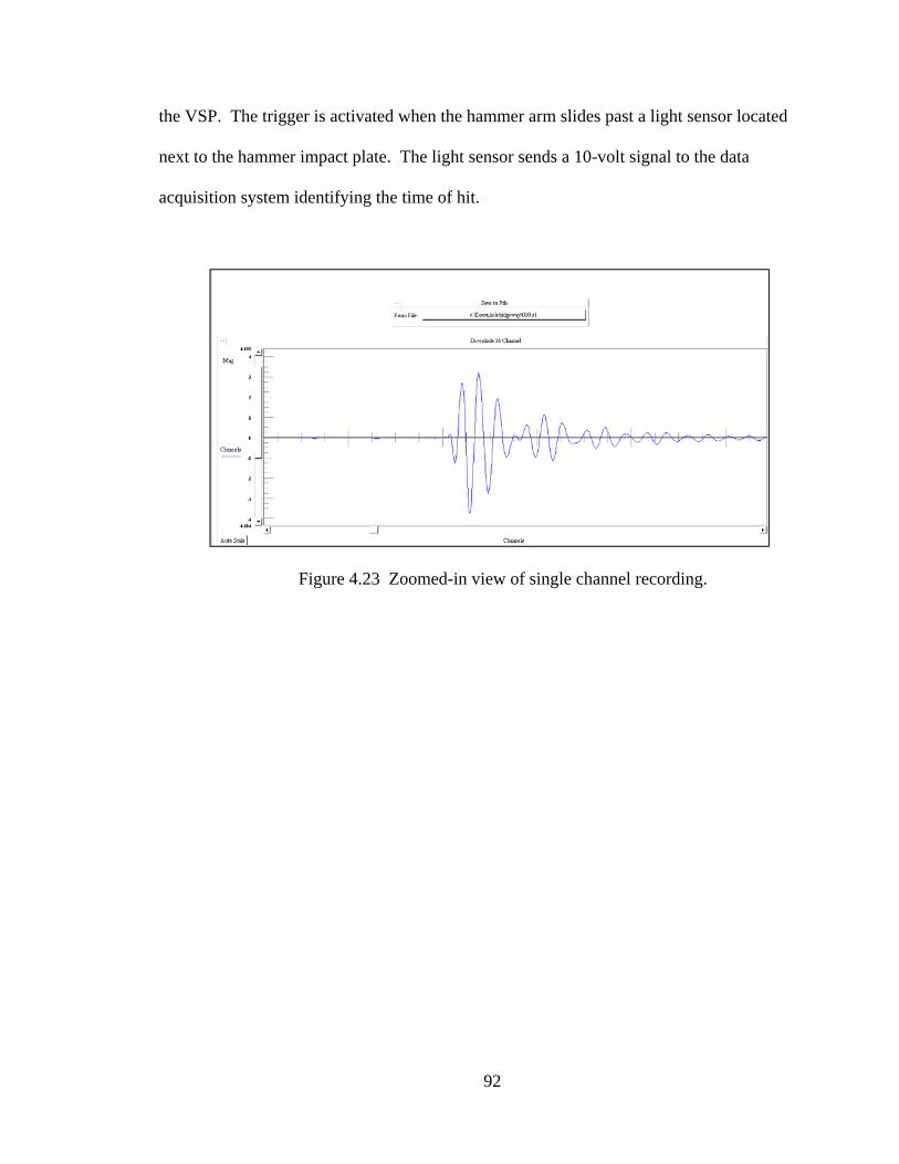
92
the VSP. The trigger is activated when the hammer arm slides past a light sensor located
next to the hammer impact plate. The light sensor sends a 10-volt signal to the data
acquisition system identifying the time of hit.
Figure 4.23 Zoomed-in view of single channel recording.

93
Chapter 5. Signal Processing
Chapter 4 discussed the procedures and equipment used in the collection of Rayleigh
surface wave data. The data collected by the instrumentation is a digitized sample of the
continuous signals recorded. These digitized copies are then used for the methods
described in Chapter 3. The following chapter discusses important signal processing
techniques, such as frequency resolution, aperture selection, coherency, spatial aliasing
and higher mode resolution, which need to be understood and followed in order for the
methods of Chapter 3 to produce reliable results to be used in inversion.
5.1 Frequency Resolution
Chapter 3 showed that MASW relies on phase information to determine Rayleigh
dispersion. This requires all collected data to be transformed from the time domain to the
frequency domain via the Discrete Fourier transform (DFT). Care must be taken when
extracting the information for frequencies that may not be represented by the DFT. The
DFT is defined as (Bracewell, 1965)
1
0
0,1,..... 1( ) ( )exp 2
0,1,..... 1
N v NvF v f jNNτ
τ πττ
−
=
= −⎛ ⎞= −⎜ ⎟ = −⎝ ⎠∑ (5.1.1)
Where
( ) ( )of f t tτ τ= + Δ (5.1.2)
Δt is the sampling interval, ( )of t tτ+ Δ is the sample at time τΔt adjusted from the initial
recording time to, N is the total number of samples and the quantity v/N is analogous to
frequency measured in cycles per sampling interval. From Equation (5.1.1) it can seen
94
that the individual frequency resolution in the DFT is directly controlled by the
relationship v/N where the total number of samples N is dependent on the sampling
interval Δt. If sampling intervals used in testing are not chosen appropriately, frequency
resolution can suffer.
Two problems arise when the sampling rate is not chosen properly. The first
problem is known as aliasing. Aliasing occurs when under-sampling causes a signal to
appear aliased into a signal of lower frequency content. The frequency limit where
aliasing occurs is governed by the Nyquist frequency, which is defined as
1
2 2s
nyff
t= =
Δ (5.1.3)
where fs sampling frequency, which is the inverse of the sampling interval Δt. The
Nyquist frequency establishes the maximum resolvable frequency due to the chosen
sampling frequency. Any frequency information collected beyond the Nyquist frequency
is considered aliased and should be considered unreliable.
The second problem is that the individual frequency step resolution may not allow
for a specific individual frequency to be obtained. Individual frequency resolution is
controlled by
sffN
Δ = (5.1.4)
where Δf is the frequency step. When a signal is transferred from the time domain to the
frequency domain via the DFT, information is only available for the frequencies that are
a multiple of Δf. All information pertaining to a specific frequency that is not a multiple

95
of Δf will be integrated into the next closest frequency step. This problem can be
overcome by padding the end of a signal with zero values prior to the application of the
DFT. This is done in order to increase the value of N and thus decrease the value of Δf.
For this research a sampling frequency of 640 points per second was selected along with
a 10 second recording window resulting in a frequency step of 0.1 Hz.
5.2 Welch’s Averaged Modified Periodogram
The f-k method of Section 3.4 applies Welch’s method in order to minimize variance
in the power spectrum estimates used in the calculation of spatio-spectral correlation
matrix. Welch’s method is a spectral averaging technique that partitions a time domain
signal into a specified number of overlapping segments. The overlapping segments are
then windowed and the discrete Fourier transform, Equation (3.3.1), is applied to each
window. Welch’s method then averages the DFT from each segment in order to
minimize variance in the power spectrum estimate.
When applying Welch’s method in Section 3.4 it is important that the correct number
of windows and window size be chosen. Just as sampling frequency is important to
frequency resolution so are the window choices. Recall that Welch’s method splits a
time domain signal into a specified number of overlapping segments. The size of the
overlap is user-defined but typical examples use a 50% overlap. The overlap used is due
to the fact that most window functions afford more influence to the center of the data set.
Figure 5.1 displays three common window functions along with their matching kernels.
The kernel is the inverse Fourier transform of the window and helps to indentify the
spectral leakage associated with the windowing function. The best window function to
use can depend on the information required from the data set. For this research the
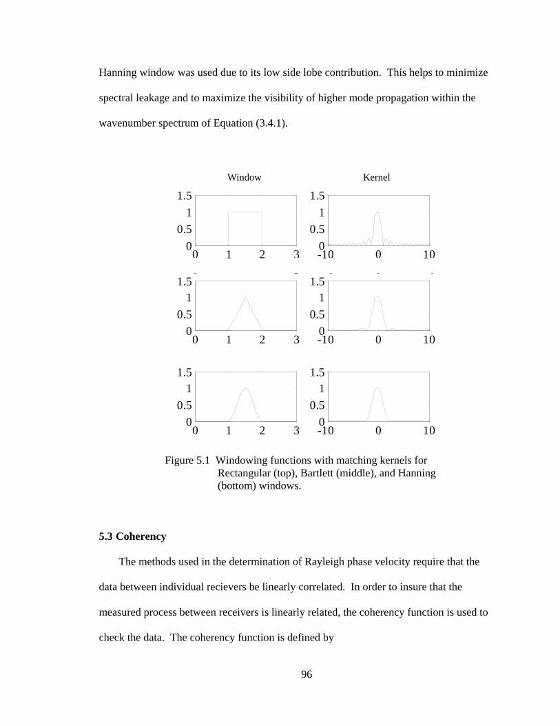
96
Hanning window was used due to its low side lobe contribution. This helps to minimize
spectral leakage and to maximize the visibility of higher mode propagation within the
wavenumber spectrum of Equation (3.4.1).
Figure 5.1 Windowing functions with matching kernels for Rectangular (top), Bartlett (middle), and Hanning (bottom) windows.
5.3 Coherency
The methods used in the determination of Rayleigh phase velocity require that the
data between individual recievers be linearly correlated. In order to insure that the
measured process between receivers is linearly related, the coherency function is used to
check the data. The coherency function is defined by
0 1 2 30
0.51
1.5
-10 0 100
0.51
1.5
0 1 2 30
0.51
1.5
-10 0 100
0.51
1.5
0 3 0 0 0
0 1 2 30
0.51
1.5
-10 0 100
0.51
1.5
Window Kernel
97
*
2( ) ( )
( )( ) ( )
m n S Sn m
m n
m m n n
S SS S
S S S S
Y Yf
Y Y
ω ωγ
ω ω= (5.3.1)
where Y is the cross power between receivers Sn and Sm from Equation (3.3.2) and the *
denotes the complex conjugate. If the data recorded at the individual recievers is exactly
linear related then Equation (5.3.1) results in a coherency value of 1. Low coherency
values can result from low signal-to-noise ratio, body-wave interference, and near-field
effects. For this research only coherency values of 0.90 and higher are accepted from the
MASW method.
5.4 Apertures
Due to the fact that propagating waves vary in space and time, sensor arrangements
have a significant influence on the ability of an array to capture propagating energy. It is
the arrangement of sensors within an array that determines the aperture used in the
collection of propagating energy. The two-dimensional Fourier transform of a spatial-
temporal signal s(x,t) can be written as (Johnson and Dudgeon, 1993)
( , ) ( , ) exp( )exp( )S k s x t j t jkx dxdtω ω∞ ∞
−∞ −∞
= −∫ ∫ (5.4.1)
where k is the wavenumber, ω is the circular frequency, x is the position, t is the time and
j is the imaginary number. Inserting the uniform plane wave equation
( , ) exp( ( ))o
os x t j t k xω= − (5.4.2)
98
into Equation (5.4.1) yields
( , ) exp( ( ) ) exp( ( ) )ooS k j t j k k x dxdtω ω ω
∞ ∞
−∞ −∞
= − − −∫ ∫ (5.4.3)
where ko and ωo represent a particular wavenumber and frequency. If unlimited temporal
and spatial data could be collected then the wave field of Equation (5.4.3) would be given
by the two-dimensional impulse function in f-k space as
( , ) ( ) ( )ooS k k k dkdω δ ω ω δ ω
∞ ∞
−∞ −∞
= − −∫ ∫ (5.4.4)
Equation (5.4.4) is an ideal smoothing kernel. In reality, experimental measurements are
neither perfect nor infinite in length. The finite wave field is therefore a convolution over
wavenumber between the Fourier transform of the field and the aperture smoothing
function
( , ) ( , ) ( )Z k S k W kω ω= (5.4.5)
where S(k,ω) is determined from the two-dimensional DFT and W(k) is defined as
1
0( ) ( ) exp( )
m
n nn
W k w x jkx−
=
= ∑ (5.4.6)
where w(x) is the aperture function, also termed applied weights, that help to control the
shape of the ASF and m is the total number of sensor locations. For the case of a single
plane wave propagating along x due to a source waveform s(t), the frequency-
wavenumber spectrum can be written as

99
( , ) ( ) ( )oZ k S W k kω ω= − (5.4.7)
From Equation (5.4.7) it can be seen that when k is equal to ko then
( , ) ( ) (0)oZ k S Wω ω= (5.4.8)
Along this path the output spectrum equals the signal spectrum. For all other values of k,
the signal spectrum is multiplied by a value less than one resulting in less power in a
particular f-k pair.
The ASF’s main lobe is used as a beam to point, algorithmically, the array’s spatial
filter toward desired f-k pairs. Plane waves of frequency f traveling along the array with
wavenumber k will result in peaks within the steered response power spectra. It is the
shape of the ASF that is most important when analyzing results from the f-k method. If a
linear array is used in the collection of data with uniformly spaced sensors, the resulting
ASF would look like a typical aperture function with a main lobe peak and small
decreasing side lobes as seen in Figure 5.2. If a non-uniform array is used, the ASF
suffers from higher side lobes resulting from aliasing effects from gaps within the
coarray.

100
Figure 5.2 ASF for a linear array of length 102 ft. with uniform spacing of 3 ft. (solid line), non uniform array x = [0 2 4 7 10 14 20 26 34 42 52 62 72 87 102] ft. (dashed line).
5.5 Spatial Aliasing
Spatial aliasing is the result of insufficient sampling along a space axis that results in
an aperture function becoming distorted. To avoid spatial aliasing in a particular
direction, the minimum spatial separation contained in the coarray must be (Zywicki,
1999)
minmin 2
d λ≤ (5.5.1)
where d is the minimum spatial separation and λ is the wavelength. Recalling Equation
(2.9.3) , the maximum wavenumber that can be contained in the wavefield without
aliasing is therefore
maxmin min
2kd
π πλ
= = (5.5.2)
Wavenumber k
101
where kmax is analogous to the Nyquist frequency. When uniform spacing is used, the
sampling rate is constant resulting in identifiable aliasing criteria within the ASF.
However, available space and equipment limits may not allow for a uniform spacing to
occur. Non-uniform arrays are designed so that a given array length can be achieved with
less sensors. A problem with non-uniform arrays is that they contain spatial gaps in their
coarray. These gaps results in uneven spatial sampling resulting in no true aliasing
present in the ASF. In cases where true aliasing lobes do not exist, large side lobes
demarcate aliasing criteria. It is these side lobes which are the focus of concern when
interpreting multiple-mode Rayleigh waves.
For spatial arrays, the lag domain is summarized by the coarray, which represents
all the spatial lags contained in an array. The coarray is defined as
1 1
( ) ( )S S
m nm n
C x xχ δ= =
= −∑∑ (5.5.3)
where xm and xn are the positions of individual sensors, χ is the lag distance between
sensors m and n, and S is the total number of sensors in the array. From Equation (5.5.3)
it can be seen that the zero lag will result in the highest coarray value, which equals the
total number of sensors in the array. For a uniform array this results in a linear decline in
coarray value with increasing lag. Figure 5.3 graphically displays the coarray for a 102-ft
array with uniform 3 ft spacing and Figure 5.4 displays the coarray for the 102-ft non-
uniform spacing array of Hebeler (2001). The uniform array contains larger values in the
coarray for individual lags than that of the non-uniform array, resulting in an ASF with
lower side lobe contributions (Figure 5.5).

102
The coarray can prove to be helpful when determining the optimal geometry for a
non-uniform array. The magnitude squared of the ASF is equal to the Fourier transform
of the coarray which is defined as (Johnson and Dudgeon, 1993)
2( ) ( ) exp( )W k c jkx
χχ= ∑ (5.5.4)
Once an array geometry is chosen, the resulting ASF can be determined from Equation
(5.5.4). This allows for an optimization procedure for determining an optimal ASF.
Figure 5.3 Coarray for 102-ft array with uniform 3-ft spacing.
By optimizing Equation (5.5.4) for a given array length with n number of sensors,
side lobe heights can be minimized, allowing for a more reliable identification of true
mode peaks in the steered response. The genetic algorithm discussed in Section 2.11 was
used to search for a non-uniform 15-sensor array of at least 100-ft that provided
-100 -50 0 50 100-10
0
10
20
30
40Coarray
Lag Distance (ft)
# of
Lag
s in
Coa
rray

103
minimum spectral leakage. The 100 ft minimum length was chosen due to the depth of
penetration desired. The actual depth of penetration a wavelet can achieve is not certain
until inversion is completed. Some researchers suggest the depth of penetration is
typically equal to one half or two thirds the wavelength (Ballard, 1964; Lai and Rix,
1998; Foti, 2000; and Hebeler, 2001). The results of the GA provided a non-uniform
array that matched those used in both previous studies from Hebeler (2001) and Zarrabi
(2005). Equation (5.5.5) displays the geometry of the 15-sensor non uniform array. The
resulting kmax value of Equation (5.5.2) is
[0 2 4 7 10 14 20 26 34 42 52 62 72 87 102] ftx = (5.5.5)
Figure 5.4 Coarray for 102-ft array with non uniform spacing.
-100 -50 0 50 100-10
-5
0
5
10
15
20y
Lag Distance (ft)
# of
Lag
s in
Coa
rray

104
Figure 5.5 Array smoothing function for uniform and non-uniform arrays.
5.6 Wavenumber Spectrum
The results of Equation (3.4.1) used in the f-k method to determine Rayleigh
phase velocity produce a wavenumber spectrum that displays the power in particular f-
k pairs. If a single-mode Rayleigh wave is propagating along the non-uniform array of
Equation (5.5.5) the resulting wavenumber spectrum would be that of Figure 5.6.
For multiple-mode propagation the resulting wavenumber spectrum should contain
multiple peaks located at the wavenumber k values of the propagating modes.
For this research, the f-k method was applied to synthetic multiple-mode Rayleigh
waveforms generated using Equation (2.3.4) with a duration of 10 seconds. Figure 5.7
displays a 5-Hz, 1-second window of the individual modal propagation at each sensor
-1.5 -1 -0.5 0 0.5 1 1.50
0.2
0.4
0.6
0.8
1
Wavenumber k
Nor
mal
ized
Pow
er
UniformNon Uniform

105
along the array. Figure 5.8 displays the waveform generated by the superposition of
the propagating modes.
Figure 5.6 Wavenumber spectrum for single mode propagation.
Figure 5.7 One-second window of synthetic time histories for
individual Rayleigh wave mode propagation for each receiver in a non-uniform array. Frequency = 5 Hz with k = 0.2 (dashed) and k = 0.75 (solid).
Wavenumber k
0 0.2 0.4 0.6 0.8 1-2
0
2 x = 0
0 0.2 0.4 0.6 0.8 1-2
0
2 x = 2
0 0.2 0.4 0.6 0.8 1-2
0
2 x = 4
0 0.2 0.4 0.6 0.8 1-2
0
2 x = 7
0 0.2 0.4 0.6 0.8 1-2
0
2 x = 10
0 0.2 0.4 0.6 0.8 1-2
0
2 x = 14
0 0.2 0.4 0.6 0.8 1-2
0
2 x = 20
0 0.2 0.4 0.6 0.8 1-2
0
2 x = 26
0 0.2 0.4 0.6 0.8 1-2
0
2 x = 34
0 0.2 0.4 0.6 0.8 1-2
0
2 x = 42
0 0.2 0.4 0.6 0.8 1-2
0
2 x = 52
0 0.2 0.4 0.6 0.8 1-2
0
2 x = 62
0 0.2 0.4 0.6 0.8 1-2
0
2 x = 72
0 0.2 0.4 0.6 0.8 1-2
0
2 x = 87
0 0.2 0.4 0.6 0.8 1-2
0
2 x = 102

106
Figure 5.8 One-second window of synthetic time histories of
mulit-mode, k1 = 0.2 and k2 = 0.75, Rayleigh wave propagation for frequency of 5 Hz for each receiver in a non-uniform array.
The resulting wavenumber spectra were then plotted to indentify the individual
modes of propagation for individual frequencies. Figure 5.9 displays the wavenumber
spectrum resulting from the application of the f-k method to the synthetic signals of
Figure 5.8. Two peaks are clearly defined at k values representing the propagating
wavenumber values of 0.2 and 0.75. For this result it appears that both modes are
equally dominant in the wavenumber spectrum. By adding a third mode of
propagation, k = 0.5, the wavenumber spectrum results in a clearly dominant mode of
propagation for k = 0.5 (see Figure 5.10). The propagating modes for k1 and k3 are
still clearly visible within the power spectrum, however, side lobe levels are increasing
to sizes larger than those of the true propagating modes.
0 0.2 0.4 0.6 0.8 1-2
0
2 x = 0
0 0.2 0.4 0.6 0.8 1-2
0
2 x = 2
0 0.2 0.4 0.6 0.8 1-2
0
2 x = 4
0 0.2 0.4 0.6 0.8 1-2
0
2 x = 7
0 0.2 0.4 0.6 0.8 1-2
0
2 x = 10
0 0.2 0.4 0.6 0.8 1-2
0
2 x = 14
0 0.2 0.4 0.6 0.8 1-2
0
2 x = 20
0 0.2 0.4 0.6 0.8 1-2
0
2 x = 26
0 0.2 0.4 0.6 0.8 1-2
0
2 x = 34
0 0.2 0.4 0.6 0.8 1-2
0
2 x = 42
0 0.2 0.4 0.6 0.8 1-2
0
2 x = 52
0 0.2 0.4 0.6 0.8 1-2
0
2 x = 62
0 0.2 0.4 0.6 0.8 1-2
0
2 x = 72
0 0.2 0.4 0.6 0.8 1-2
0
2 x = 87
0 0.2 0.4 0.6 0.8 1-2
0
2 x = 102

107
Figure 5.9 Wavenumber spectrum for multi-mode, k1 = 0.2 and k2 = 0.75, Rayleigh wave propagation for frequency of 5 Hz.
0 0.2 0.4 0.6 0.8 1 1.2 1.4 1.60
0.1
0.2
0.3
0.4
0.5
0.6
0.7
0.8
0.9
1
Wavenumber k
Nor
mal
ized
Pow
er

108
Figure 5.10 Wavenumber spectrum for multi-mode, k1 = 0.2 and k2 = 0.5, and k3 = 0.75 Rayleigh wave propagation for frequency of 5 Hz.
These large side lobes can be mistaken as propagating modes. Therefore, care must be
taken when choosing k values for true modal propagation. By modeling the wavenumber
response of a linear array the resulting side lobe contributions can be identified, thus
reducing the error in modal identification
When a recorded signal contains plane waves of a given frequency f and modal
wavenumbers ki, then the resulting wavenumber spectrum is a superposition of
propagating modes multiplied by a complex steering vector as described in Section 3.4.
0 0.2 0.4 0.6 0.8 1 1.2 1.4 1.60
0.1
0.2
0.3
0.4
0.5
0.6
0.7
0.8
0.9
1
Wavenumber k
Nor
mal
ized
Pow
er

109
This is best explained in complex notation by defining the temporal response of a
receiver from a multi-mode propagating plane wave as
[ ] [ ],1 1 ,( , ) exp ( ) exp ( )r r o r r M o M rs x t A j t K x A j t K xω ω= − + + − (5.6.1)
where xr is the position coordinate of receiver r in the array, t is the time, Ar,m is the
amplitude of the mth mode at reciever r, ωo is the circular frequency, Km is the
wavenumber of propagation for the mth mode, and M is the total number of propagating
modes. In summation form this reduces to
[ ],1
( , ) exp ( )M
i i m o m im
s x t A j t K xω=
= −∑ (5.6.2)
The cross power between receivers can then be calculated by
[ ] [ ], ,1 1
( , ) ( , )* exp ( ) exp ( )M M
c r c n o n c r m o m rn m
s x t s x t A j t K x A j t K xω ω= =
= − − −∑ ∑ (5.6.3)
where the * represents complex conjugate. Combining summations results in
[ ], ,1 1
( , ) ( , )* exp ( )M M
c r c n r m m r n cn m
s x t s x t A A j K x K x= =
= −∑∑ (5.6.4)
where the frequency dependence ωot in the exponential has been eliminated. Applying
the weighted steering vector of Section 3.4, the wavenumber spectrum can then be
calculated by
110
( ) [ ] ( ), ,1 1 1 1
( ) exp exp ( ) expN M M N
c c c n r m m r n c r rc n m r
P k w jkx A A j K x K x w jkx= = = =
= − −∑ ∑∑ ∑ (5.6.5)
where wc is the vector of applied weights for each receiver c, N is the total number of
receivers, and k is the range of wavenumbers used in the wavenumber spectrum. When
the summations are combined Equation (5.6.5) reduces to
[ ]( ), ,1 1 1 1
( ) exp ( ) ( )N N M M
c r c n r m m r n cc r n m
P k w w A A j K k x K k x= = = =
= − − −∑∑ ∑∑ (5.6.6)
From Equation (5.6.6) it can be determined that when an individual k is equal to
the true propagating wavenumbers K and n is equal to m the result of the exponential
component is equal to one. This results in Equation (5.6.6) retaining all the power from
Equation (5.6.4) at K. When n does not equal m the exponential value is less than one
resulting in a decrease in the cross power.
Equation (5.6.6) can therefore be used as a model for comparison between
theoretical and experimental results. An inversion of Equation (5.6.6) should determine
the true modal propagation values. However, Equation (5.6.6) assumes complete modal
participation in all receivers within an array, which is not necessarily the case in
experimental results.
There are three types of interference that influence the shape of the wavenumber
spectrum apart from the true modal propagation. The first is low-frequency noise
propagation. Low-frequency noise is a common occurrence in areas containing soft
sediments such as the Mississippi embayment. Figure 5.11 displays the Fourier
amplitude spectrum of a single receiver from a MASW experimental test site. The

111
spectrum contains sharp high-amplitude peaks for frequencies above 20 Hz providing
good signal-to-noise ratios for high frequencies. Below the 20-Hz frequency level the
signal to noise ratio becomes poor thus resulting in poor spectral resolution.
Figure 5.11 Fourier amplitude spectrum for all experimental frequencies.
A zoomed plot of the Fourier amplitude spectrum for frequencies ranging from 0 to
20 Hz can be seen in Figure 5.12. From this figure it can be seen that frequencies below
10 Hz are completely indistinguishable from one another. This is due mostly to the small
energy imparted by the source at low frequencies compared to that of the ground noise
levels. A plot of the coherency (see Section 5.3) between the receivers from the
20 40 60 80 100
0
2
4
6
8
10
12
14
16
Frequency (Hz)
Four
ier A
mpl
itude

112
experiment is plotted in Figure 5.13. It can be seen that for frequencies below 20 Hz the
coherency value begins to drop off sharply.
Figure 5.12 Fourier amplitude spectrum for experimental frequencies from 3.75 to 20 Hz.
The resulting 3.75-Hz wavenumber spectrum of the experimental test from Figure
5.11 through Figure 5.13 is plotted in Figure 5.14. The test results are compared to the
synthetic wavenumber spectrum obtained from Equation (5.6.6) using a single
propagating wavenumber K of 0.013. The experimental data results in a wavenumber
spectrum with a much higher power distribution over the majority of the spectrum. This
5 10 15 200
0.5
1
1.5
2
2.5
3
3.5
4
Frequency (Hz)
Four
ier A
mpl
itude

113
is most likely due to a poor signal-to-noise ratio that results in high side lobe
contribution.
Figure 5.13 Coherency values for experimental frequencies.
The high energy distribution could also be the result of body wave interference
caused by the source. When a source is close to an array and a shallow layer with high
impedance exists within the medium, body waves from the source can reflect and refract
off the layer and can have significant influence on receiver response. This could also
explain why the energy distribution is reflected at higher k values, resulting in lower
propagation speeds.
0 20 40 60 80 1000.4
0.5
0.6
0.7
0.8
0.9
1
1.1
Frequency (Hz)
Coh
eren
cy
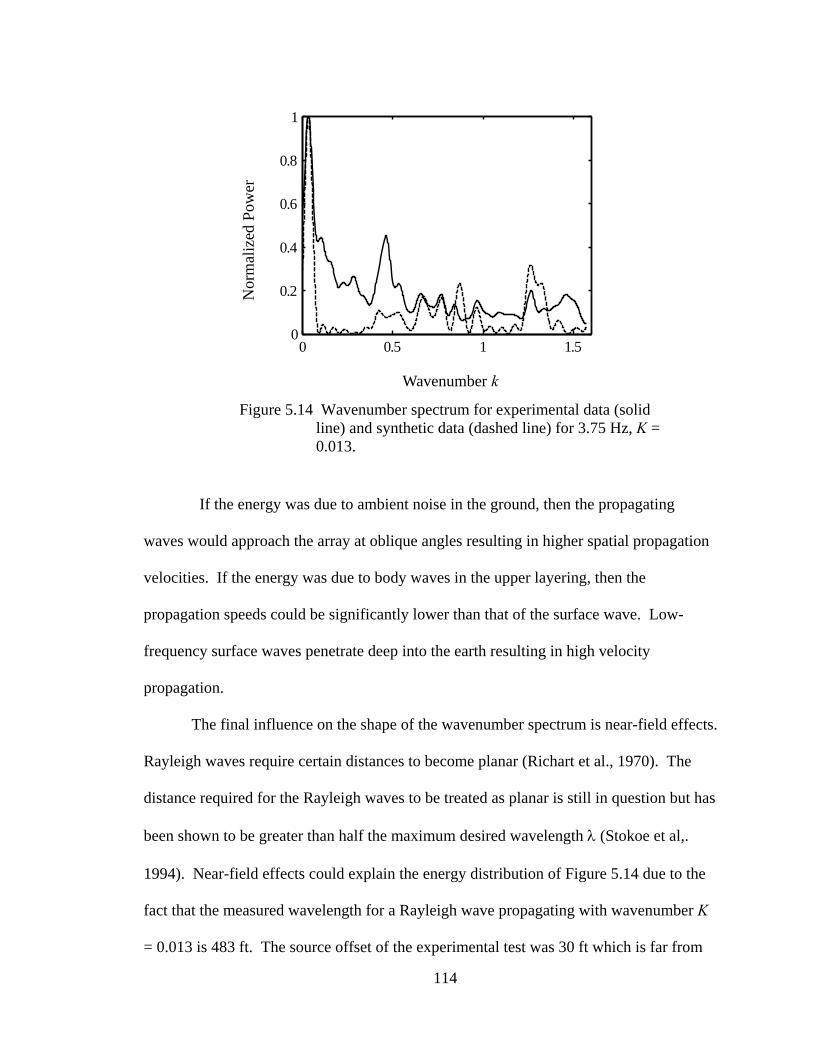
114
Figure 5.14 Wavenumber spectrum for experimental data (solid
line) and synthetic data (dashed line) for 3.75 Hz, K = 0.013.
If the energy was due to ambient noise in the ground, then the propagating
waves would approach the array at oblique angles resulting in higher spatial propagation
velocities. If the energy was due to body waves in the upper layering, then the
propagation speeds could be significantly lower than that of the surface wave. Low-
frequency surface waves penetrate deep into the earth resulting in high velocity
propagation.
The final influence on the shape of the wavenumber spectrum is near-field effects.
Rayleigh waves require certain distances to become planar (Richart et al., 1970). The
distance required for the Rayleigh waves to be treated as planar is still in question but has
been shown to be greater than half the maximum desired wavelength λ (Stokoe et al,.
1994). Near-field effects could explain the energy distribution of Figure 5.14 due to the
fact that the measured wavelength for a Rayleigh wave propagating with wavenumber K
= 0.013 is 483 ft. The source offset of the experimental test was 30 ft which is far from
Wavenumber k
Nor
mal
ized
Pow
er
0 0.5 1 1.50
0.2
0.4
0.6
0.8
1

115
one-half the wavelength. In fact the length of the source offset plus the array length is
less than one-third the wavelength.
5.7 Higher-Mode Resolution
One of the goals of this research was to clearly identify individual modes of
propagation for an accurate inversion of Rayleigh wave dispersion. As seen in the
section above accurate determination of higher-mode propagation can be a challenge
when other factors of wave propagation are involved. However, for typical dispersion
curves obtained from experimental results, the dominance of higher-mode wave
propagation is typically for frequencies above 30 Hz. Recalling the Fourier amplitude
spectrum of Figure 5.11, the MASW method with a harmonic source provides good high
frequency resolution above 20 Hz.
The main obstacle is in identifying the dominant mode’s true modal value. If a
MASW experiment was conducted for the site of Case 2 (Figure 2.18) the experimental
dispersion curve may result in a dominant higher mode for frequencies above 90 Hz. If a
multi-mode inversion was conducted and the frequencies above 90 Hz were associated
with the second mode, the results would be inaccurate due to the fact that the frequencies
above 90 Hz fall on the third mode.
The reason for higher-mode dominance within Rayleigh dispersion is not certain.
The two likely possibilities are attenuation and near-field effects. It was shown in
Section 2.8 that higher-mode Rayleigh waves penetrate deeper into a media. It is also
known that surface wave attenuation is most sensitive to shear wave dissipation (Kennett,
2001). If the quality factor Q for shear waves increases with depth, then at some
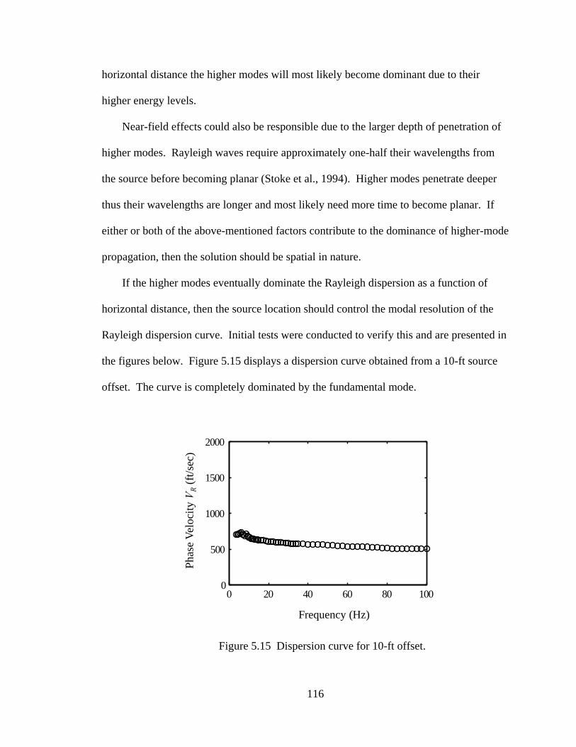
116
horizontal distance the higher modes will most likely become dominant due to their
higher energy levels.
Near-field effects could also be responsible due to the larger depth of penetration of
higher modes. Rayleigh waves require approximately one-half their wavelengths from
the source before becoming planar (Stoke et al., 1994). Higher modes penetrate deeper
thus their wavelengths are longer and most likely need more time to become planar. If
either or both of the above-mentioned factors contribute to the dominance of higher-mode
propagation, then the solution should be spatial in nature.
If the higher modes eventually dominate the Rayleigh dispersion as a function of
horizontal distance, then the source location should control the modal resolution of the
Rayleigh dispersion curve. Initial tests were conducted to verify this and are presented in
the figures below. Figure 5.15 displays a dispersion curve obtained from a 10-ft source
offset. The curve is completely dominated by the fundamental mode.
Figure 5.15 Dispersion curve for 10-ft offset.
0 20 40 60 80 1000
500
1000
1500
2000
Frequency (Hz)
Phas
e Ve
loci
ty V
R(f
t/sec
)

117
Figure 5.16 through Figure 5.19 display some of the wavenumber spectra used in the
construction of the dispersion curve. Each wavenumber spectrum is plotted along with
the synthetic spectrum based on Equation (5.6.6) for the k value of the main peak. It can
be seen that the synthetic spectrum matches well for the 18.75 and 31.25 Hz frequencies.
As the frequency increases, the width of the main lobe for the experimental data
increases. The reason for the increase in main lobe width is not certain but could be due
to propagating wavenumbers that are aligned close to one another. However, as source
offset distance increases, sharper more distinct peaks will begin to form in the
waevenumber spectrum.
Figure 5.21 displays the dispersion curve obtained using a 30-ft source offset. There
is clearly a higher mode jump for frequencies above 90 Hz. By investigating the
wavenumber spectra used in the construction of Figure 5.21 a hypothesis can be drawn as
to why the widening of the peaks occurs at higher frequencies.

118
Figure 5.16 Wavenumber spectrum for experimental data (solid line) and synthetic data (dashed line) for 18.75 Hz, k = 0.178.
Figure 5.17 Wavenumber spectrum for experimental data (solid line) and synthetic data (dashed line) for 31.25 Hz, k = 0.337.
Wavenumber k
Nor
mal
ized
Pow
er
0 0.5 1 1.50
0.2
0.4
0.6
0.8
1
Wavenumber k
Nor
mal
ized
Pow
er
0 0.5 1 1.50
0.2
0.4
0.6
0.8
1

119
Figure 5.18 Wavenumber spectrum for experimental data (solid line) and synthetic data (dashed line) for 55 Hz, k = 0.636.
Figure 5.19 Wavenumber spectrum for experimental data (solid
line) and synthetic data (dashed line) for 80 Hz, k = 0.988.
Wavenumber k
Nor
mal
ized
Pow
er
0 0.5 1 1.50
0.2
0.4
0.6
0.8
1
Wavenumber k
Nor
mal
ized
Pow
er
0 0.5 1 1.50
0.2
0.4
0.6
0.8
1

120
Figure 5.20 Wavenumber spectrum for experimental data (solid line) and synthetic data (dashed line) for 100 Hz, k = 1.255.
Figure 5.21 Dispersion curve for 30-ft offset.
As the frequency increases from 27.5 Hz a secondary peak begins to form to the left
of the main peak (Figure 5.22). This could be the formation of the next higher-mode but
Wavenumber k
Nor
mal
ized
Pow
er
0 0.5 1 1.50
0.2
0.4
0.6
0.8
1
0 20 40 60 80 1000
500
1000
1500
2000
Frequency (Hz)
Phas
e Ve
loci
ty V
R(f
t/sec
)

121
this is still not certain. This trend continues until 75 Hz when these assumed higher mode
peaks begin to rapidly diminish (Figure 5.23 and Figure 5.24). If these secondary peaks
were chosen as higher modes and added to the dispersion curve of Figure 5.21, the
resulting dispersion would look like that of Figure 5.25. If Figure 5.25 is accurate it
could then be assumed that the mode jump at 90 Hz must be the third or even higher
mode. However, care must be taken when associating secondary peaks with higher
modes. Side lobes resulting from spatial aliasing can produce the same effects when
chosen as secondary peaks.

122
Figure 5.22 Wavenumber spectrums for frequencies of 27.5 to 45 Hz for 30-ft offset.
0 0.5 1 1.50
0.5
127.5Hz
0 0.5 1 1.50
0.5
128.75Hz
0 0.5 1 1.50
0.5
130Hz
0 0.5 1 1.50
0.5
131.25Hz
Nor
mal
ized
Pow
er
0 0.5 1 1.50
0.5
137.5Hz
0 0.5 1 1.50
0.5
140Hz
0 0.5 1 1.50
0.5
142.5Hz
0 0.5 1 1.50
0.5
145Hz
Wavenumber k
Nor
mal
ized
Pow
er

123
Figure 5.23 Wavenumber spectrums for frequencies of 55 to 80 Hz for 30-ft offset.
0 0.5 1 1.50
0.5
155Hz
0 0.5 1 1.50
0.5
157.5Hz
0 0.5 1 1.50
0.5
160Hz
0 0.5 1 1.50
0.5
162.5Hz
Nor
mal
ized
Pow
er
0 0.5 1 1.50
0.5
172.5Hz
0 0.5 1 1.50
0.5
175Hz
0 0.5 1 1.50
0.5
177.5Hz
0 0.5 1 1.50
0.5
180Hz
Wavenumber k
Nor
mal
ized
Pow
er
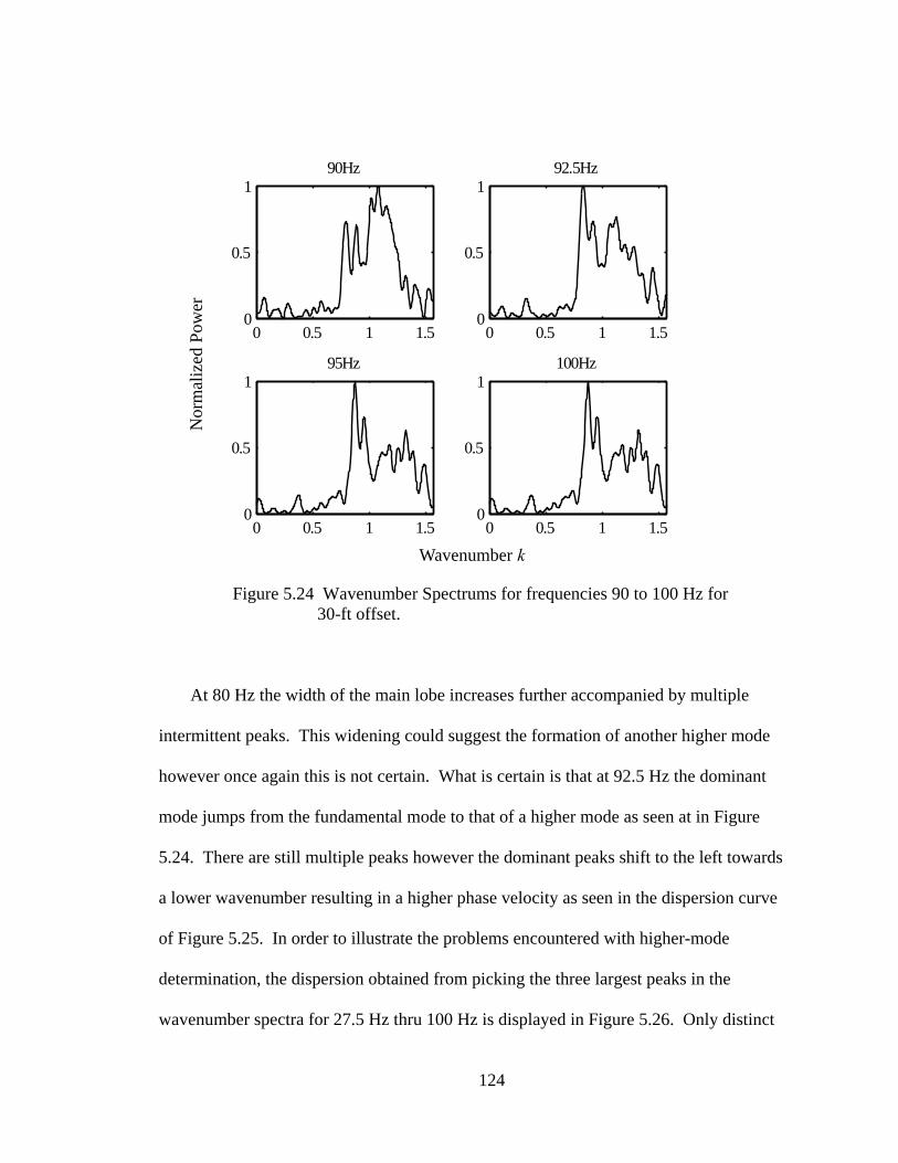
124
Figure 5.24 Wavenumber Spectrums for frequencies 90 to 100 Hz for
30-ft offset.
At 80 Hz the width of the main lobe increases further accompanied by multiple
intermittent peaks. This widening could suggest the formation of another higher mode
however once again this is not certain. What is certain is that at 92.5 Hz the dominant
mode jumps from the fundamental mode to that of a higher mode as seen at in Figure
5.24. There are still multiple peaks however the dominant peaks shift to the left towards
a lower wavenumber resulting in a higher phase velocity as seen in the dispersion curve
of Figure 5.25. In order to illustrate the problems encountered with higher-mode
determination, the dispersion obtained from picking the three largest peaks in the
wavenumber spectra for 27.5 Hz thru 100 Hz is displayed in Figure 5.26. Only distinct
0 0.5 1 1.50
0.5
190Hz
0 0.5 1 1.50
0.5
192.5Hz
0 0.5 1 1.50
0.5
195Hz
0 0.5 1 1.50
0.5
1100Hz
Wavenumber k
Nor
mal
ized
Pow
er

125
peaks were chosen whose magnitude was higher than 0.4. This value was chosen in
order that no peaks were associated with side lobes resulting from the ASF itself. It is
clear that the dispersion of Figure 5.26 offers no certainty as to the true modal phase
velocities.
Figure 5.25 Dispersion curve for 30-ft offset with suspected next-higher mode.
Figure 5.26 Dispersion curve for 30-ft offset with suspected next two higher modes.
Frequency (Hz)
Phas
e Ve
loci
ty V
R(f
t/sec
)
0 20 40 60 80 1000
500
1000
1500
2000
Frequency (Hz)
Phas
e Ve
loci
ty V
R(f
t/sec
)
0 20 40 60 80 1000
500
1000
1500
2000

126
The results of the above test do not produce a high level of confidence for the
identification of higher modes. The only information from the wavenumber spectrum
that can be used with any certainty is the dominant peak except in frequency ranges of
low coherency. For this research only the dominant peaks were used in the construction
of experimental dispersion curves. In order to identify as many modes as possible,
incremental source offsets were used. If the increased width of the main lobe is due to
either attenuation or near-field effects, changes in offset distance should result in changes
in the dominate mode of propagation. For near offsets the fundamental modes will most
likely control depending on the length of the array. This is due to the fact that the
wavelength of the fundamental mode is the shortest and should take less time to become
planar. However, if an array is long enough a higher mode could eventually dominate
over a majority of the array length thus resulting in a dominant higher mode within the
wavenumber spectrum. For a short array the higher mode may still be experiencing near-
field effects and thus explain the wide main lobe response in the wavenumber spectrum.
Once a higher mode becomes planar there should be a distinct split in the peaks that
represent the propagating modes.
The domination of the higher modes could be the result of higher Q values as a
function of depth. In Section 2.8, the response of displacement eigenfunctions was
plotted for individual modal values. It was shown that the majority of the energy
distribution for the fundamental mode was located near the surface. Higher modal energy
is distributed more evenly with depth and thus would attenuate less if Q values increased
with depth.
127
The results section will show that the determination of multiple modes for a given
frequency can be achieved through multiple source offsets. Each offset produces an
individual Rayleigh dispersion curve that is used in combination with all others obtained
at different source offsets. The resulting dispersion curve is a composite mapping of the
individual propagating modes as a function of frequency.
5.8 Downhole Arrival Times
The determination of soil velocities from downhole testing requires that arrival times
be picked from a VSP for use in calculating the interval velocities. Figure 5.27 displays
the chosen arrival times for an example VSP where the arrival times are depicted by a +
sign located at the beginning of the energy arrival. It is imperative that the arrival time be
chosen as close as possible to the first energy arrival in order to minimize error. If the
main peaks are chosen as the arrival times two errors are incurred. The first is the
velocity of the uppermost layer will be highly underestimated due to the resulting larger
denominator of Equation (4.3.1). The second error is incurred due to the signal shape
changing with depth. As depth increases the signal can pass through multiple layers that
result in the signal’s shape becoming altered. Signals at different depths can have
varying pulse widths with the main peak shifted significantly. Reflections from lower
layers can also cause significant disturbances in signals located in the layers above.
The cross correlation of signals can also be used to determine the time difference
between signal arrivals. By determining the time shift required to maximize the cross
correlation function, the velocity between the two intervals can then be determined by
dividing the depth interval by the time shift. This method can also produce large errors
when the signal shape of one depth interval does not match that of the other. Large peaks
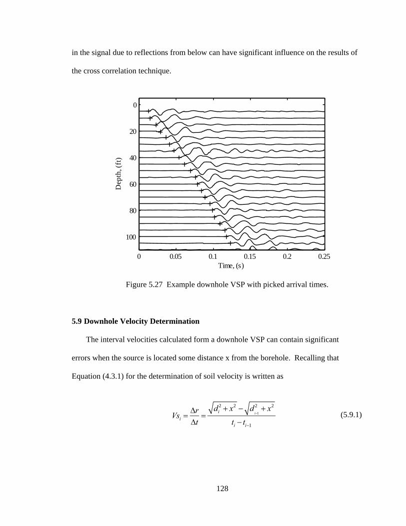
128
in the signal due to reflections from below can have significant influence on the results of
the cross correlation technique.
Figure 5.27 Example downhole VSP with picked arrival times.
5.9 Downhole Velocity Determination
The interval velocities calculated form a downhole VSP can contain significant
errors when the source is located some distance x from the borehole. Recalling that
Equation (4.3.1) for the determination of soil velocity is written as
1
2 2 2 2
1
iii
i i
d x d xrVst t t
−
−
+ − +Δ= =
Δ −(5.9.1)
0 0.05 0.1 0.15 0.2 0.25
0
20
40
60
80
100
Time, (s)
Dep
th, (
ft)

129
The numerator of Equation (5.9.1) simply calculates the difference in ray path distance ri
between the source and two receivers (Figure 5.28). This difference is then divided by
the change in arrival time for the determination of layer velocity.
Figure 5.28 Downhole schematic.
For shallow layers the propagating signal can spend significantly more time in one layer
than Equation (5.9.1) would suggest. To illustrate this consider a source located x = 5
feet from the borehole and the depth interval between sensors is 5 feet. If the arrival
time at the interface of Layers 1 and 2 is 0.00900 seconds and the arrival time at the
interface of Layers 2 and 3 is 0.014815 seconds then the resulting ray path difference
would be
1
2 2 2 2 2 2 2 22 10 5 5 5 4.1093r d x d x ftΔ = + − + = + − + = (5.9.2)
and the resulting velocity for Layer 2
r1
r2r3
x
d1
d2
d3
Source
Borehole
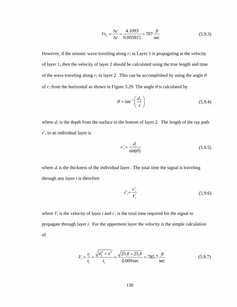
130
24.1093 707
0.005815 secr ftVst
Δ= = =
Δ (5.9.3)
However, if the seismic wave traveling along r2 in Layer 1 is propagating at the velocity
of layer 1, then the velocity of layer 2 should be calculated using the true length and time
of the wave traveling along r2 in layer 2. This can be accomplished by using the angle θ
of r2 from the horizontal as shown in Figure 5.29. The angle θ is calculated by
1 2tan dx
θ − ⎛ ⎞= ⎜ ⎟⎝ ⎠
(5.9.4)
where d2 is the depth from the surface to the bottom of layer 2. The length of the ray path
r`i in an individual layer is
`sin( )
ii
drθ
= (5.9.5)
where di is the thickness of the individual layer. The total time the signal is traveling
through any layer i is therefore
`` i
ii
rtV
= (5.9.6)
where Vi is the velocity of layer i and t`i is the total time required for the signal to
propagate through layer i. For the uppermost layer the velocity is the simple calculation
of
2 2
111
1 1
25 25785.7
0.009sec secd x ft ftr ftV
t t+ +
= = = = (5.9.7)
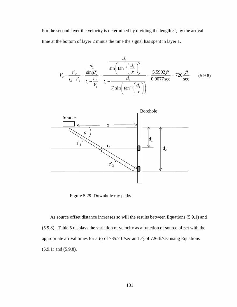
131
For the second layer the velocity is determined by dividing the length r`2 by the arrival
time at the bottom of layer 2 minus the time the signal has spent in layer 1.
2
1 22
22
1 12 12 2
11 11
sin tan` 5.5902sin( ) 726`` 0.0077sec sec
sin tan
dddxr ft ftV r dt t t t
V dVx
θ−
−
⎛ ⎞⎛ ⎞⎜ ⎟⎜ ⎟⎝ ⎠⎝ ⎠= = = = =
− − −⎛ ⎞⎛ ⎞
⎜ ⎟⎜ ⎟⎝ ⎠⎝ ⎠
(5.9.8)
Figure 5.29 Downhole ray paths
As source offset distance increases so will the results between Equations (5.9.1) and
(5.9.8) . Table 5 displays the variation of velocity as a function of source offset with the
appropriate arrival times for a V1 of 785.7 ft/sec and V2 of 726 ft/sec using Equations
(5.9.1) and (5.9.8).
r2
x
d2
SourceBorehole
d1
θ
r`2
r`1

132
Table 5. Computed layer velocity as a function of source offsets, V1 = 785.7 ft/sec and V2 = 726 ft/sec.
Source Offset
Distance (ft)
Arrival time
t1 (sec)
Arrival time
t2 (sec)
Equation (5.9.1) V2
(ft/sec)
Equation (5.9.8) V2
(ft/sec)
5 0.009000 0.014815 707 726 7 0.010949 0.016175 690 726 9 0.013104 0.017827 669 726
Table 6 presents how this error is further compounded with a high velocity in the
upper layer. The arrival times are adjusted for a V1 of 1000 ft/sec and V2 of 726 ft/sec
Table 6. Layer velocity as a function of source offsets, V1 = 1000 ft/sec and V2 = 726 ft/sec.
Source Offset
Distance (ft)
Arrival time
t1 (sec)
Arrival time
t2 (sec)
Equation (5.9.1) V2
(ft/sec)
Equation (5.9.8) V2
(ft/sec)
5 0.007071 0.01329 661 726 7 0.008602 0.01451 610 726 9 0.010296 0.01599 555 726
For a multiple layer case with equally spaced depth intervals Equation (5.9.8) can be
simplified to the following
1nn
n
rV for nt
= = (5.9.9)
1
11
nn
n iin
nrV V for nt
−
−
= − >∑ (5.9.10)
133
where Vn is the velocity at layer n, rn is the distance from the source to the sensor in layer
n, tn is the arrival time at layer n, Vi is the velocity of an individual layer above layer n.
Once the top layer velocity is determined from Equation (5.9.9) each successive layer
velocity can then be determined using Equation (5.9.10) . These equations can be easily
programmed into a computer algorithm or a spreadsheet for automatic calculation of
layer velocities.

134
Chapter 6. Experimental Results
6.1 Results for Covington, TN
The first site tested was at a Tennessee Department of Transportation maintenance
facility located in Covington, TN at coordinates 35°33'33.77" North by 89°36'58.14"
West (Figure 6.1). This site was chosen due to the existence of a 200-ft cased borehole
remaining from a previous research project (Pezeshk and Zarrabi, 2005). Both MASW
and ReMi tests were conducted.
Figure 6.1 Tennessee Department of Transportation maintenance facility located in Covington, TN.
The downhole velocity profile used for this test was adopted from Ge et al., (2007)
and is displayed in Figure 6.2. Ge et al., (2007) used a waveform matching technique for
the determination of the vertical seismic profile. The technique uses synthetic waveforms
generated from the method outlined by Wu, (1983) to match the experimental results
collected from downhole measurements.
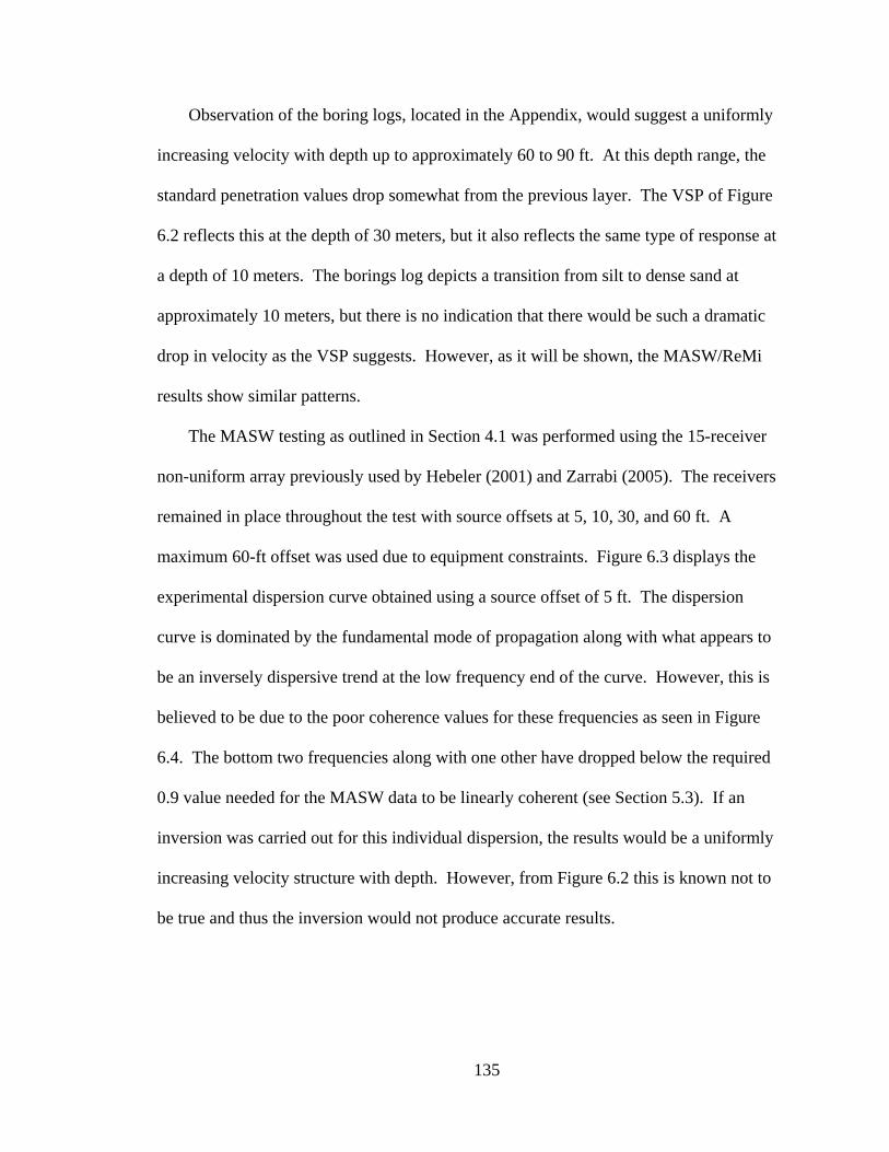
135
Observation of the boring logs, located in the Appendix, would suggest a uniformly
increasing velocity with depth up to approximately 60 to 90 ft. At this depth range, the
standard penetration values drop somewhat from the previous layer. The VSP of Figure
6.2 reflects this at the depth of 30 meters, but it also reflects the same type of response at
a depth of 10 meters. The borings log depicts a transition from silt to dense sand at
approximately 10 meters, but there is no indication that there would be such a dramatic
drop in velocity as the VSP suggests. However, as it will be shown, the MASW/ReMi
results show similar patterns.
The MASW testing as outlined in Section 4.1 was performed using the 15-receiver
non-uniform array previously used by Hebeler (2001) and Zarrabi (2005). The receivers
remained in place throughout the test with source offsets at 5, 10, 30, and 60 ft. A
maximum 60-ft offset was used due to equipment constraints. Figure 6.3 displays the
experimental dispersion curve obtained using a source offset of 5 ft. The dispersion
curve is dominated by the fundamental mode of propagation along with what appears to
be an inversely dispersive trend at the low frequency end of the curve. However, this is
believed to be due to the poor coherence values for these frequencies as seen in Figure
6.4. The bottom two frequencies along with one other have dropped below the required
0.9 value needed for the MASW data to be linearly coherent (see Section 5.3). If an
inversion was carried out for this individual dispersion, the results would be a uniformly
increasing velocity structure with depth. However, from Figure 6.2 this is known not to
be true and thus the inversion would not produce accurate results.

136
Figure 6.2 Downhole VSP and shear wave velocity chart for Covington, TN (adopted from Ge et al., 2007)
The source was then moved to a 10-ft offset and the MASW test was repeated. The
results were very similar to the 5-ft offset test with the only difference being a slight
change over the low frequencies (Figure 6.5). Once again the coherency values for the
lowest frequencies drop below the 0.9 threshold.
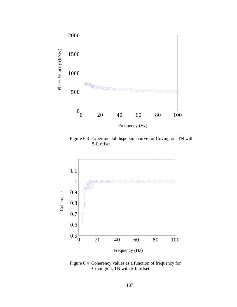
137
Figure 6.3 Experimental dispersion curve for Covington, TN with 5-ft offset.
Figure 6.4 Coherency values as a function of frequency for Covington, TN with 5-ft offset.
0 20 40 60 80 1000
500
1000
1500
2000
Frequency (Hz)
Phas
e Ve
loci
ty (f
t/sec
)
0 20 40 60 80 1000.5
0.6
0.7
0.8
0.9
1
1.1
Frequency (Hz)
Coh
eren
ce
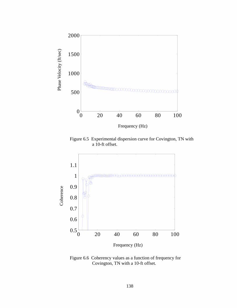
138
Figure 6.5 Experimental dispersion curve for Covington, TN with a 10-ft offset.
Figure 6.6 Coherency values as a function of frequency for Covington, TN with a 10-ft offset.
0 20 40 60 80 1000
500
1000
1500
2000
Frequency (Hz)
Phas
e Ve
loci
ty (f
t/sec
)
0 20 40 60 80 1000.5
0.6
0.7
0.8
0.9
1
1.1
Frequency (Hz)
Coh
eren
ce

139
The reason for the low coherence at low frequencies is most likely due to a poor
signal-to-noise ratio. The noise spectrum of an individual receiver is displayed in Figure
6.7. It can be seen that for frequencies below approximately 20 Hz the signal-to-noise
ratio begins to diminish rapidly.
Once the source was moved to a 30-ft offset, the dispersion curve began to reflect
higher-mode propagation as shown in Figure 6.8 along with the corresponding coherency
plot in Figure 6.9. At 90 Hz there is a jump in the dispersion curve from the fundamental
mode to that of a higher mode. The actual mode number is unknown and to assume that
it is the next higher mode would be careless as will be shown shortly. The coherence
values remain as they have been in the previous offsets with poor values at low
frequencies. Once the source offset is moved to 60-ft, better assumptions as to actual
mode number values can be made.
Figure 6.7 Fourier amplitude spectrum for MASW test data (blue) and ground noise (red).
10 20 30 40 50 60 70 80 90 100
50
100
150
200
250
Frequency (Hz)
Four
ier A
mpl
itude

140
Figure 6.8 Experimental dispersion curve for Covington, TN with 30-ft offset.
Figure 6.9 Coherency values as a function of frequency for Covington, TN with a 30-ft offset.
0 20 40 60 80 1000
500
1000
1500
2000
Frequency (Hz)
Phas
e Ve
loci
ty (f
t/sec
)
0 20 40 60 80 1000.5
0.6
0.7
0.8
0.9
1
1.1
Frequency (Hz)
Coh
eren
ce

141
Figure 6.10 displays the dispersion curve results for the MASW test with a 60-ft
offset. The resulting dispersion curve contains some key characteristics for
understanding the multiple mode dispersion relationship. Multiple-mode jumps appear in
the dispersion curve over specific frequency ranges. Recalling the dispersion curves
from the previous offset tests, it can be seen that as the source offset increases, higher
mode participation begins to dominate the dispersion curve. This would suggest that
either the higher modes need more time to develop, and thus are more susceptible to near
field effects, or higher modes attenuate at a lower rate than that of the fundamental mode.
This could result from higher Q values at the larger depths where higher modes penetrate.
Figure 6.10 Experimental dispersion curve for Covington, TN with 60-ft offset.
Another characteristic of the dispersion curve that is related to the higher mode
propagation is the rise in the curve at low frequencies. At approximately 10 Hz the curve
0 20 40 60 80 1000
500
1000
1500
2000
Frequency (Hz)
Phas
e Ve
loci
ty (f
t/sec
)

142
begins to become inversely dispersive until it reaches a peak at 15 Hz and then returns to
a normally dispersive trend. This effect is the result of simultaneous multiple-mode
propagation along the array and is referred to as the effective phase velocity as discussed
in Section 2.7. It is now clear from Figure 6.10 that the jump in the dispersion curve at
90 Hz was not the second mode. In fact it appears likely that the jump corresponds to the
fourth mode. Notice how the coherency values at the lower frequencies increased for the
60 ft offset (Figure 6.11). This would support the near-field theory that the lower
frequency, longer wavelengths need more time to develop and become planar.
Figure 6.11 Coherency values as a function of frequency for Covington, TN with 60-ft offset.
The ReMi method (see Section 3.5) was used to provide dispersion information for
the low frequencies where coherency values from the MASW method were below the 0.9
threshold. Twelve sensors were spaced eight meters apart in order to sample large
0 20 40 60 80 1000.5
0.6
0.7
0.8
0.9
1
1.1
Frequency (Hz)
Coh
eren
ce

143
wavelengths corresponding to low-frequency propagation. Only twelve sensors were used
due to spatial constraints. The ReMi method took advantage of the low-frequency noise
shown in the Fourier amplitude spectrum of Figure 6.7 for the construction of the p-f
spectrum shown in Figure 6.12. Slowness values are chosen along the bottom of the
energy spectrum in order to obtain values associated with the surface waves propagating
most directly along the array of receivers. The dispersion curves from both the MASW
and ReMi methods were combined to form a composite dispersion curve (Figure 6.13).
The composite dispersion curve should ensure that both the MASW and ReMi
dispersions agree well at their point of intersection. It is possible that energy may not
propagate directly along the line of receivers, especially if only ambient noise is used.
The resulting dispersion from the ReMi method could result in a curve that lies above
that of the MASW method. However this can be overcome by creating a source at the
end of the receivers to ensure energy propagation along the line.

144
Figure 6.12 Frequency-slowness spectrum obtained from ReMi for Covington, TN.
Inversion of the composite dispersion was carried out by the Genetic Algorithm of
Zarrabi (2005) using the forward method of Lai and Rix (1999). A system of 10 soil
layers was used in inversion where each layer thickness and its respective shear-wave
velocity were allowed to vary. Ten layers where chosen based on the layering
information from the boring log and the VSP of Figure 6.2. The results of the inversion
are displayed in Figure 6.14 with the corresponding velocity profile shown in Figure
6.15.
The composite experimental dispersion is represented by the triangular shapes and
the resulting multi-mode theoretical dispersion by the colored shapes. These results show
how volatile multi-mode dispersion can be. Notice the “mode pinching” (see Section
Frequency (Hz)
Slow
ness
(sec
/m)
0.0 20.0
0.01
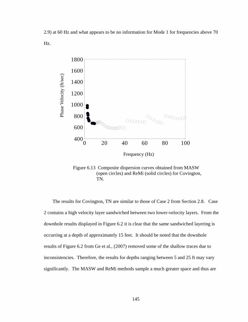
145
2.9) at 60 Hz and what appears to be no information for Mode 1 for frequencies above 70
Hz.
Figure 6.13 Composite dispersion curves obtained from MASW (open circles) and ReMi (solid circles) for Covington, TN.
The results for Covington, TN are similar to those of Case 2 from Section 2.8. Case
2 contains a high velocity layer sandwiched between two lower-velocity layers. From the
downhole results displayed in Figure 6.2 it is clear that the same sandwiched layering is
occurring at a depth of approximately 15 feet. It should be noted that the downhole
results of Figure 6.2 from Ge et al., (2007) removed some of the shallow traces due to
inconsistencies. Therefore, the results for depths ranging between 5 and 25 ft may vary
significantly. The MASW and ReMi methods sample a much greater space and thus are
0 20 40 60 80 100400
600
800
1000
1200
1400
1600
1800
Frequency (Hz)
Phas
e Ve
loci
ty (f
t/sec
)

146
more of an averaged result. However, the results should show similarities due to the slow
nature of soil deposits and the short 102 ft length of the MASW array.
A final remark should be made on the portion of the curve between 60 and 80 Hz.
While the experimental and theoretic values differ, it is believed that the theoretical
values represent effective phase velocities due to the presence of the multiple mode
propagation. If the source were to be moved further away, these effective velocities
would more than likely jump to a dominant mode. However, equipment constraints did
not allow for this to be confirmed.
The resulting shear wave velocity profiles of the downhole and MASW/ReMi
methods are compared in Figure 6.15 and Figure 6.16. Figure 6.15 displays the
comparison for the first 100 ft and Figure 6.16 for the entire 165 ft. Although the
borehole reaches to 200 ft, the results of the MASW/ReMi only penetrate to 165 ft. The
velocity profile from the MASW/ReMi methods reflects the high velocity layer at 15 feet
and matches the overall trend in the velocity profiles well. In fact, the velocity profile of
Figure 6.16 reflects the low velocity layer sandwiched at 90 ft. The 100-ft average shear
wave velocity as defined by Equation (3.5-1) in NEHRP (2003) results in 829 ft/sec from
the downhole method and 758 ft/sec from the MASW/ReMi methods, which results in
only a 9% difference.
The variability in the results of the GA is displayed by the error bars in both figures.
The error bars represent the standard deviation for all solutions found by the GA with
fitness values obtained from Equation (2.11.2) that are within 10% of the minimum
fitness reached. The variability for the first 100 ft is minimal with an average standard
deviation in shear-wave velocities of 40 ft/sec. This minimum variability in solutions is
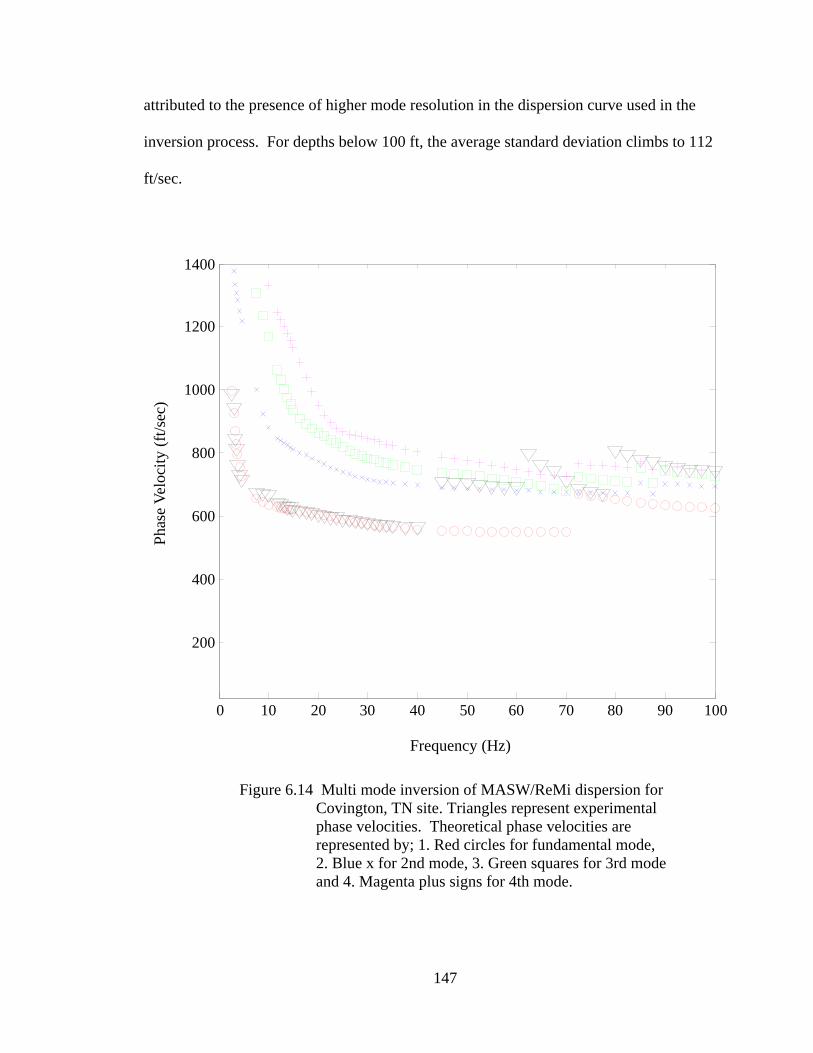
147
attributed to the presence of higher mode resolution in the dispersion curve used in the
inversion process. For depths below 100 ft, the average standard deviation climbs to 112
ft/sec.
Figure 6.14 Multi mode inversion of MASW/ReMi dispersion for Covington, TN site. Triangles represent experimental phase velocities. Theoretical phase velocities are represented by; 1. Red circles for fundamental mode, 2. Blue x for 2nd mode, 3. Green squares for 3rd mode and 4. Magenta plus signs for 4th mode.
0 10 20 30 40 50 60 70 80 90 100
200
400
600
800
1000
1200
1400
Frequency (Hz)
Phas
e Ve
loci
ty (f
t/sec
)

148
Figure 6.15 Velocity profile comparison for Covington, TN site for 100 ft..
0
5
10
15
20
25
30
35
40
45
50
55
60
65
70
75
80
85
90
95
100
0 500 1000 1500
MASW/ReMi Downhole
Dep
th (f
t)
Shear-wave Velocity (ft/sec)
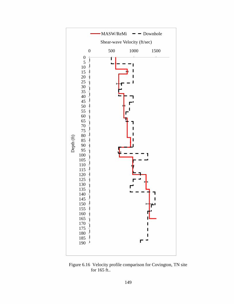
149
Figure 6.16 Velocity profile comparison for Covington, TN site for 165 ft..
05
101520253035404550556065707580859095
100105110115120125130135140145150155160165170175180185190
0 500 1000 1500
MASW/ReMi Downhole
Shear-wave Velocity (ft/sec)
Dep
th (f
t)

150
6.2 Results for Hayti, Missouri
The second site tested was located near Hayti, Missouri at coordinates 36°10'14.52“
North by 89°47'21.44" West (Figure 6.18). This site was chosen due to the presence of a
100-ft cased borehole used in consulting work. Both MASW and ReMi tests were
conducted along with a downhole test reaching 90 feet in depth.
Figure 6.17 Test site located near Hayti, Missouri.
The testing for all methods was the same as for the Covington site with the only
exception being that the source offsets were 10, 30, and 60 ft. Figure 6.18 displays the
VSP along with the resulting shear wave velocities obtained from the downhole
experiment. There is fair agreement between the VSP and the boring log located in the
Appendix. The log indicates distinct layer boundaries at depths of 10, 30, 45, 50, 60, 80,
and 90 ft. The VSP contains significant velocity changes at depths of 10, 30, 45, and 60

151
ft. Once again, there is the presence of inverse layering, which typically results in higher
mode Rayleigh wave propagation and dispersion curve fluctuation.
Figure 6.18 Downhole VSP and shear wave velocity chart for Hayti, Missouri site.
The dispersion curve for the 10-ft source offset contains what appears to be a large jump
in the dispersion curve at frequencies above 75 Hz (Figure 6.19). By inspecting the
coherency values in Figure 6.20, it can be seen that the values are all below the 0.9
threshold for frequencies above 75 Hz. It is unclear why the coherency was poor
especially since the site was a very quiet farmland with no farm equipment in use. By
inspecting the phase velocity value of the frequencies above 75 Hz, the resulting
400 600 800
0
10
20
30
40
50
60
70
80
90
0 0.1 0.2 0.3 0.4
0
10
20
30
40
50
60
70
80
90
Time (sec) Shear Wave Velocity (ft/sec)
Dep
th (f
t)
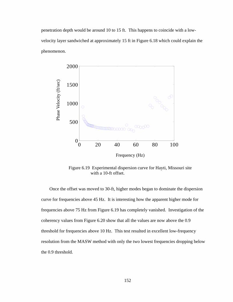
152
penetration depth would be around 10 to 15 ft. This happens to coincide with a low-
velocity layer sandwiched at approximately 15 ft in Figure 6.18 which could explain the
phenomenon.
Figure 6.19 Experimental dispersion curve for Hayti, Missouri site with a 10-ft offset.
Once the offset was moved to 30-ft, higher modes began to dominate the dispersion
curve for frequencies above 45 Hz. It is interesting how the apparent higher mode for
frequencies above 75 Hz from Figure 6.19 has completely vanished. Investigation of the
coherency values from Figure 6.20 show that all the values are now above the 0.9
threshold for frequencies above 10 Hz. This test resulted in excellent low-frequency
resolution from the MASW method with only the two lowest frequencies dropping below
the 0.9 threshold.
0 20 40 60 80 1000
500
1000
1500
2000
Frequency (Hz)
Phas
e Ve
loci
ty (f
t/sec
)

153
Figure 6.20 Coherency values as a function of frequency for Hayti, Missouri site with a 10-ft offset.
Figure 6.21 Experimental dispersion curve for Hayti, Missouri site with a 30-ft offset.
0 20 40 60 80 100
0.6
0.7
0.8
0.9
1
1.1
Frequency (Hz)
Coh
eren
ce
0 20 40 60 80 1000
500
1000
1500
2000
Frequency (Hz)
Phas
e Ve
loci
ty (f
t/sec
)

154
Figure 6.22 Coherency values as a function of frequency for Hayti, Missouri site with a 30-ft offset.
The 60-ft-offset test resulted in larger jumps in the dispersion curves as compared to
that of the 30-ft-offset test (Figure 6.23). There are also some significant scattering
effects at frequencies above 75 Hz. With the exception of a few low frequencies, all of
the coherency values of Figure 6.24 are above the 0.9 threshold, but only slightly. There
is also a small set of phase velocity values between 30 and 40 Hz that appear to be
effective phase velocities but it is not clear. The composite dispersion curve will shed
some light on this matter.
0 20 40 60 80 100
0.6
0.7
0.8
0.9
1
1.1
Frequency (Hz)
Coh
eren
ce
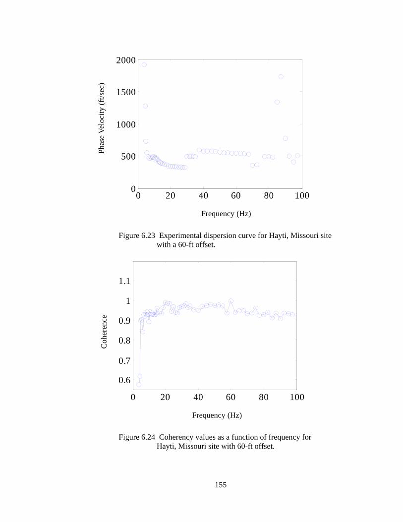
155
Figure 6.23 Experimental dispersion curve for Hayti, Missouri site with a 60-ft offset.
Figure 6.24 Coherency values as a function of frequency for Hayti, Missouri site with 60-ft offset.
0 20 40 60 80 1000
500
1000
1500
2000
Frequency (Hz)
Phas
e Ve
loci
ty (f
t/sec
)
0 20 40 60 80 100
0.6
0.7
0.8
0.9
1
1.1
Frequency (Hz)
Coh
eren
ce
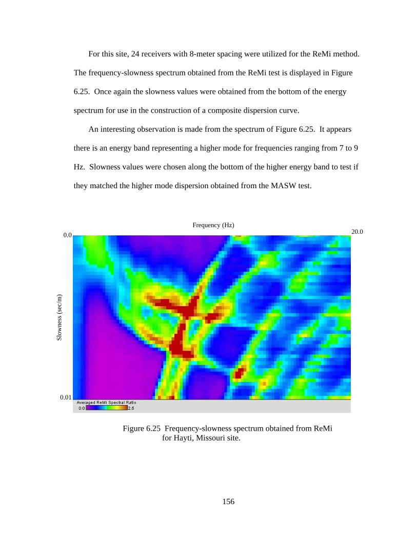
156
For this site, 24 receivers with 8-meter spacing were utilized for the ReMi method.
The frequency-slowness spectrum obtained from the ReMi test is displayed in Figure
6.25. Once again the slowness values were obtained from the bottom of the energy
spectrum for use in the construction of a composite dispersion curve.
An interesting observation is made from the spectrum of Figure 6.25. It appears
there is an energy band representing a higher mode for frequencies ranging from 7 to 9
Hz. Slowness values were chosen along the bottom of the higher energy band to test if
they matched the higher mode dispersion obtained from the MASW test.
Figure 6.25 Frequency-slowness spectrum obtained from ReMi for Hayti, Missouri site.
Frequency (Hz)
Slow
ness
(sec
/m)
0.0 20.0
0.01

157
The resulting composite dispersion from both the MASW and ReMi methods is
plotted in Figure 6.26, and includes the higher mode data from the upper energy band of
the frequency-slowness spectrum. Only points with coherency values clearly above the
0.9 threshold were used in the composite curve. Individual frequencies that did not meet
this requirement were not used.
Figure 6.26 Composite dispersion curves obtained from MASW (open circles) and ReMi (solid circles) for Hayti, Missouri site.
Inversion of the composite dispersion was carried out by the Genetic Algorithm of
Zarrabi (2005) using the forward method of Lai and Rix (1999). A system of 10 soil
layers was used in inversion where each layer thickness and its respective shear-wave
velocity were allowed to vary. Ten layers where chosen based on the layering
information from the boring log and the VSP of Figure 6.18. The results of the GA-based
Frequency (Hz)
Phas
e Ve
loci
ty (f
t/sec
)
0 20 40 60 80 1000
500
1000
1500
2000

158
inversion for the composite dispersion curve for the Missouri site are encouraging (Figure
6.27). It can be seen from the figure that all the points of both the MASW and the ReMi
dispersion match very well for all modes with the exception of the lowest frequency of
approximately 2 Hz. The higher mode ReMi dispersion matches the 3rd mode well for
frequencies between 7 and 9 Hz resulting in a high confidence in the ReMi method. The
results of the inversion are reflected in the shear wave velocity profile of Figure 6.28 for
the first 100 ft and in Figure 6.29 for depths to 200 ft. The 100-ft average shear wave
velocity from inversion is 625 ft/sec compared to 668 ft/sec for the downhole test. This
results in a 7% difference of Equation (3.5-1) in NEHRP (2003).
The error bars of Figure 6.28 are small for the shallow layers but begin to increase
below 90 ft. Below the 90 ft depth, the average standard deviation in shear-wave velocity
is 31 ft/sec. Beyond 90 ft, the average climbs to 150 ft/sec. This is could be due to the
inaccuracy involved from picking points along the p-f spectrum but is uncertain. The
higher mode participation from the ReMi method helps to minimize uncertainty for the
lower frequencies but only for the 7 to 9 Hz range. This range has a penetration depth of
approximately 90 ft. After the 90 ft penetration depth, only the fundamental mode
information contributes.

159
Figure 6.27 Multi mode inversion of MASW/ReMi dispersion for Hayti, Missouri site. Triangles represent experimental phase velocities. Theoretical phase velocities are represented by; 1. Red circles for fundamental mode, 2. Blue x for 2nd mode, 3. Green squares for 3rd mode and 4. Magenta plus signs for 4th mode.
0 10 20 30 40 50 60 70 80 90 100
200
400
600
800
1000
1200
1400
1600
1800
Frequency (Hz)
Phas
e Ve
loci
ty (f
t/sec
)
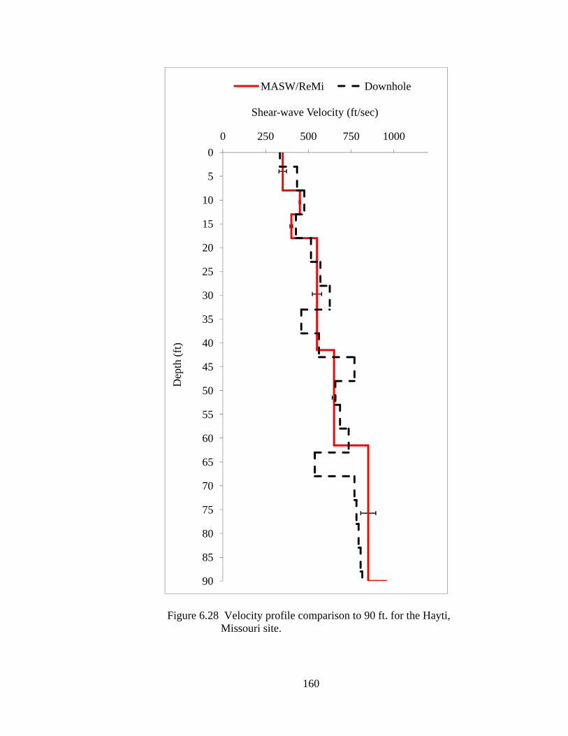
160
Figure 6.28 Velocity profile comparison to 90 ft. for the Hayti, Missouri site.
0
5
10
15
20
25
30
35
40
45
50
55
60
65
70
75
80
85
90
0 250 500 750 1000
MASW/ReMi Downhole
Shear-wave Velocity (ft/sec)
Dep
th (f
t)

161
Figure 6.29 Velocity profile comparison to 200 ft. for the Hayti, Missouri site.
05
101520253035404550556065707580859095
100105110115120125130135140145150155160165170175180185190195200
0 500 1000 1500 2000
MASW/ReMi Downhole
Shear-wave Velocity (ft/sec)
Dep
th (f
t)

162
Chapter 7. Conclusions
This study provided an improved procedure to identify multiple propagating
Rayleigh surface modes in MASW dispersion data. The improved procedure was tested
using two sites: Covington, TN and Hayti, Missouri. At those sites the procedure was
able to identify as many as four propagating modes. The moving source offset help to
overcome the problems associated with near field effects and possible lower attenuation
of higher mode propagation. By initially placing the source close to the array spread, the
fundamental mode can be mapped before higher mode propagation dominates the
dispersion curve. By moving the source to greater distances, the near-field effects can be
overcome and, as a result, higher modes identified and used in inversion.
The larger offsets also make it possible to use non-uniform arrays without the
concern of having to indentify multiple modes from smaller peaks within the
wavenumber spectrum. Multi-mode determination from the wavenumber spectrum can
lead to serious errors due to the lack of full modal participation at each receiver. By
increasing the offset, the higher modes are allowed to develop and become planar, which
allows for the accurate determination of their phase information.
The mapping of as many propagating modes as possible helps to eliminate possible
mistakes in the identification of individual modes. The inversion process is only as good
as the information it utilizes for finding the best solution; therefore, including higher
mode propagation in inversion allows for a minimum solution to be reached with little
variance between individual solutions.
163
Typical MASW procedures only provide soil profiling to around 100 ft due to the
lack of energy at low frequencies. The ReMi method has its strength at low frequencies
due to the high energy of low frequency noise propagating in the soft sediments of the
Mississippi embayment. The composite dispersion curves obtained from both the
MASW and ReMi methods allowed for a broader frequency range to be used in the
inversion process. This coupled with the higher mode resolution, provided the necessary
information to determine the shear wave velocity profiles to much greater depths than
normally possible with the MASW method alone.
The genetic algorithm used in the inversion process provided good results for both
sites when compared to downhole results. Typical inversion times are between 4 and 6
hours on a 3-GHz PC but can be much longer depending on the amount of layering
allowed and the criteria for termination. It should be noted that the Rayleigh surface
waves are not going to sample the same as the downhole method and the layering can be
simplified greatly for inversion purposes. The forward method used in the GA is a
helpful tool that can be utilized to fine-tune inversion results.
7.1 Recommendations for Future Research
In the above research a harmonic source was used to produce a continuous sinusoidal
input. This is extremely beneficial due to the fact that it provides a large data sample and
allows for spectral averaging techniques. However, recent research has shown that when
a source such as a sledge hammer is used, specific filters can be designed to identify the
individual propagating modes within a signal at specific receiver locations. This could be
very helpful in determining at what point along an array specific modes have formed and
to determine the attenuation rates associated with the individual modes.

164
More tests need to be conducted utilizing the ReMi method for the determination of
higher-mode phase velocities. The Missouri site offered a glimpse in to what could be a
very helpful strategy into mapping higher modes at very low frequencies. This would
allow for extremely large depths to be investigated with little effort. The ReMi method
utilizes a very small amount of equipment that is both portable and inexpensive compared
to other testing methods. By mapping the higher modes for low frequencies, the variation
in GA solutions could be minimized resulting in a more unique solution.
A sampling frequency of 640 points per second was used in this research for the
MASW method. While this provided a Nyquist frequency of 320 Hz, some of the
problems associated with high frequencies could be overcome by increasing the sampling
frequency to approximately 10 times the maximum frequency used. This would insure
maximum phase measurement resolution while also possibly enhancing the higher mode
visibility.

165
References
Abo-Zena, A. M. (1979). Dispersion function computations for unlimited frequency values, Geophys. J. R. Astr. Soc. 58, 91-105.
Aki, K. and P.G. Richards, (1980). Quantitative Seismology, Theory and Methods, 1, W.H. Freeman &Co., New York.
ASTM D7400-07. Standard Test Method for Downhole Seismic Testing. American Society of Testing Material Standards. West Conshohocken, Pennsylvania
Ballard, R.F. (1964). Determination of Soil Shear Moduli at Depth by In-Situ Vibratory Techneques, WES, Misc. Paper No.4-691.
Boore, D.M. and Asten, M.W. (2008). Comparison of Shear-Wave Slowness in the Santa Clara Valley, California, Using Blind Interpretations of Data from Invasive and Noninvasive Methods, Bulletin of the Seismological Society of America, 98 (4) pp. 1983–2003
Bracewell, R. (1965). The Fourier Transform and its Applications, McGraw-Hill Co.
Dunkin, J. W. (1965). Computational of modal solutions in layered elastic media at high frequencies, Bulletin of the Seismological Society of America. 55(2), 335-358.
Chen, X. (1993). A Systematic and Efficient Method of Computing Normal Modes for Multilayered Half Space.” Geophysics J. Int., Vol. 115, pp. 391-409.
Christensen, R.M. (1971). Theory of Viscoelasticity - An Introduction. Ed. Academic Press.
Ewing, W.M., Jardetzky, W.S., and Press, F. (1957). Elastic Waves in Layered Media, McGraw-Hill, 380p.
Foti, S. (2000). Multistation Methods for Geotechnical Characterization using Surface Waves, Ph.D.Dissertation, Politecnico di Torino.
Ge, J., Pujol, J., Peaeshk, S. and Stovall, S. (2007) Determination of Shallow Shear-Wave Velocity at Mississippi Embayment Sites Using Vertical Seismic Profiling Data, Bulletin of the Seismological Society of America. 97(2), 614-623.
Gucunski, N., and R. D. Wood (1991). Use of Rayleigh modes in interpretation of SASW test, Proc. of the 2nd Int. Conf. on Recent Advances in Geotechnical Earthquake Engineering and Soil Dynamics, Univ. of Missouri, Rolla, Mo., 2, 1399-1408.
Harvey, D. (1981). Seismogram synthesis using normal mode superposition: The locked mode approximation, Geophys. J. R. Astr. Soc., 66, 37-70.

166
Hebeler, G. L. (2001). Site characterization in Shelby County, Tennessee using advanced surface wave methods, Master’s Thesis, Georgia Institute of Technology.
Haskell, N.H. (1953). The Dispersion of Surface Waves in Multilayered Media , Bulletin of the Seismological Society of America, 43, pp. 17-34.
Heisey, J.S. (1982). Determination of In Situ Shear Wave Velocity from Spectral Analysis of Surface Waves, Master Thesis, The University of Texas at Austin.
Hisada, Y. (1994). An Efficient Method for Computing Green’s Functions for a LayeredHalf-Space with Sources and Receivers at Close Depths, Bulletin of the Seismological Society of America, 84(5), 1456-1472.
Hisada, Y. (1995). An Efficient Method for Computing Green’s Functions for a Layered Half-Space with Sources and Receivers at Close Depths (Part 2), Bulletin of the Seismological Society of America, 85(4), 1080-1093.
Horike, M. (1985). Inversion of Phase Velocity of Long-Period Microtremors to the S-Wave Velocity Structure Down to the Basement in Urbanized Areas, Journal of Phys. Earth, 33, pp. 59-96.
Idriss, I.M, and Sun, J.I., (1992) Users Manual for SHAKE91, Center for Geotechnical Modeling Department of Civil Environmental Engineering, University of California Davis.
Johnson, D.H., and D.E. Dudgeon, (1993). Array Signal Processing – Concepts and Techniques, PTR Prentice Hall, Inc., pp. 533.
Kennett, B.L.N. (1983),. Seismic wave propagation in a stratified media, Cambridge University Press.
Kennett, B.L.N. (2001). The Seismic Wavefield Volume 1: Introduction and Theoretical Development, Cambridge University Press.
Knopoff, L. (1952). On Rayleigh Wave Velocities, Bulletin of the Seismological Society of America, 42, pp. 307-308.
Lai, C. G., and G. J. Rix (1998). Simultaneous inversion of Rayleigh phase velocity and attenuation for near-surface site characterization”, Research Report, National Science Foundation and U.S. Geological Survey, Georgia Institute of Technology.
Lamb, H. (1904). On the Propagation of Tremors over the Surface of an Elastic Solid, Philisophical Transactions of the Royla Society, London, Ser. A, Vol. 203 pp. 1-42.
Liu, H., Maier, R.L., and Warrick, R.E. (1996), An Improved Air-Powered Impulsive Shear-Wave Source, Bulletin of the Seismological Society of America, 86, pp. 530-537.

167
Louie, J. N. (2001). Faster, better: shear-wave velocity to 100 meters depth from refraction microtremor arrays”, Bulletin of the Seismological Society of America. 91, 347–364.
Love A.E.H. (1911). Some problems of geodynamics, Cambridge Un. Press
Mooney, H.M., and Bolt, B.A. (1966), Dispersive Characteristics of the First Three Rayleigh Modes for a Single Surface Layer, Bulletin of the Seismological Society of America, 56, pp. 43-67.
Nazarian, S. (1984). In Situ Determination of Elastic Moduli of Soil Deposits and Pavement Systems by Spectral Analysis of Surface Waves Method, Ph.D. Dissertation, The University of Texas at Austin.
Nazarian, S. and K.H. II Stokoe, (1984). Use of Surface Waves in Pavement Evaluation, Transportation Research Record, 1070, pp. 132-144.
NEHRP, (2003). Recommendations and Provisions for Seismic Regulations for New Buildings and Other Structures, FEMA 450-1 Part 1: Provisions
Park, C.B., R.D. Miller, and J. Xia, (1999). Multimodal Analysis of High Frequency Surface Waves, The Symposium on the Application of Geophysics to Engineering and Environmental Problems, Conference Proceedings, March 14-18, Oakland, CA, 115-121.
Pezeshk, S., and M. Zarrabi (2005) A New Inversion Procedure for Spectral Analysis of Surface Waves Using a Genetic Algorithm, The Bulletin of the Seismological Society of America. 95(5), October 2005.
Rayleigh, Lord (1885). On Waves Propagated Along the Plane Surface of an Elastic Solid, London Mathematical Society Proc., 17, pp. 4-11
Richart F.E. Jr, Hall, J.R., and Woods R.D. (1970). Vibrations of Soils and Foundations, Prentice Hall, New Jersey.
Rix, G. J., K. H. Stokoe II, and J. M. Roesset (1991). Experimental study of factors affecting the spectral analysis of surface waves method, Research Report 1123-5, Center for Transportation Research, The University of Austin Texas.
Rix, G.J., and C.G. Lai, (1998). Simultaneous Inversion of Surface Wave Velocity and Attenuation, Geotechnical Site Characterization, Edited by P.K. Robertson and P.W. Mayne, 1, pp. 503-508, Proceedings of the First International Conference on Site Characterization – ISC ’98, Atlanta, Georgia, 19-22 April.
Rix, G. J., and C. G. Lai (1999). MATLAB forward solution, Free Computer Programs on the Website of Civil Engineering Department, Georgia Institute of Technology http://www.ce.gatech.edu/~grix/surface_wave.html
Rix, G.J. (2000). Site Characterization Using Surface Waves. Short Course Notes.

168
Rix, G.J., C.G. Lai, M.C. Orozco, G.L. Hebeler, and V. Roma, (2001). Recent Advances in Surface Wave Methods for Geotechnical Site Characterization, XV International Conference on Soil Mechanics and Geotechnical Engineering, Istanbul.
Sànchez-Salinero, I. (1987). Analytical Investigation of Seismic Methods Used for EngineeringApplications. Ph.D. Dissertation, The University of Texas at Austin, pp. 401.
Schwab, F., and L. Knopoff (1971). Surface waves on multilayered inelastic media, The Bulletin of the Seismological Society of America. 61(4), 893-912.
Stokoe, K.H., G.W. Wright, A.B. James, and M.R. Jose (1994). Characterization of Geotechnical Sites by SASW Method in Geophysical Characterization of Sites, Edited R. D. Woods, International Science Publisher, New Hampshire
Thomson, W.T. (1950). Transmission of Elastic Waves through a Stratified Solid, Journal of Applied Physics, 21, pp. 89-93.
Thorson, J. R., and J. F. Claerbout (1985). Velocity-stack and slant-stack stochastic inversion, Geophysics 50, 2727–2741.
Thrower, E. N. (1965). The Computation of the dispersion elastic waves in layered media, Journal of Sound Vibration, 2(3), 210-226.
Tokimatsu, K. Tamura, S., and H. Kojima, (1992). Effects of Multiple Modes on Rayleigh Wave Dispersion. Journal of Geotechnical Engineering, 118(10), October, pp. 1529-1543.
Tokimatsu, K., K. Shinzawa, and S. Kuwayama (1992). Use of Short Period Microtremors for VS Profiling, Journal of Geotechnical Engineering, 118(10), October, pp. 1544-1558.
Tokimatsu, K. (1995). Geotechnical Site Characterization Using Surface Waves, Proceedings, First International Conference on Earthquake Geotechnical Engineering IS-Tokyo ’95, Tokyo, Balkema, Rotterdam, pp. 1333-1368.
Viktorov I.A. (1967). Rayleigh and Lamb Waves: physical theory and applications, Plenum Press, New York
Watson, T. H. (1970). A note on fast computation of Rayleigh wave dispersion in the layered elastic half space, Bulletin of the Seismological Society of America. 60(1), 161-166.
Welch, P.D. (1967). The Use of Fast Fourier Transform for the Estimation of Power Spectra: A Method Based on Time Averaging Over Short, Modified Periodograms, IEEE Trans. Audio Electroacoustics, AU-15, pp.70-73.
Wu, R.C. (1983). Frequency Domain Computation of Synthetic Vertical Seismic Profiles, Master Thesis, Texas A&M University

169
Zarrabi, M (2005). A New Procedure for Estimation of Shear Wave Velocity Profiles Using Multi Station Spectral Analysis of Surface Waves, Regression Line Slope, and Genetic Algorithm Methods, Ph.D. Dissertation, The University of Memphis.
Zywicki, D.J. (1999). Advanced Signal Processing Methods Applied to Engineering Analysis of Seismic Surface Waves, Ph.D. Dissertation, Georgia Institute of Technology.
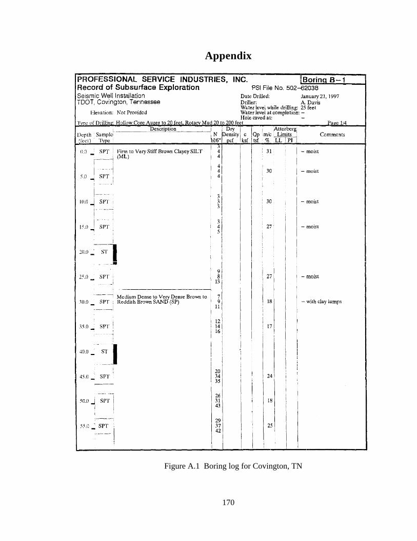
170
Appendix
Figure A.1 Boring log for Covington, TN

171
Figure A.2 Boring log for Covington, TN
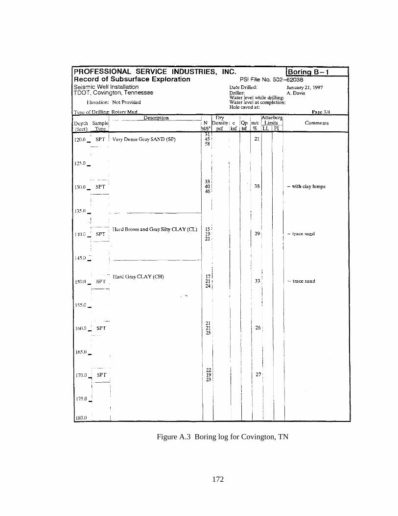
172
Figure A.3 Boring log for Covington, TN
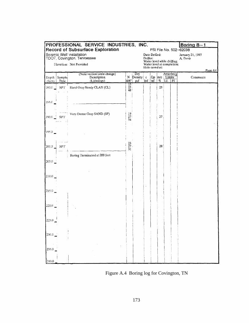
173
Figure A.4 Boring log for Covington, TN

174
Figure A.5 Boring log for Hayti, Missouri
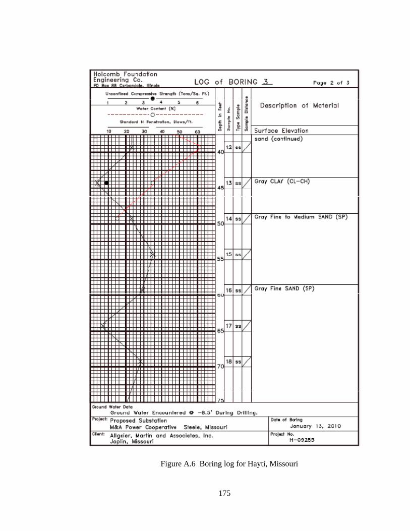
175
Figure A.6 Boring log for Hayti, Missouri

176
Figure A.7 Boring log for Hayti, Missouri