an improved method for simulation of vehicle vibration
TRANSCRIPT

University of Bath
PHD
An Improved Method for Simulation of Vehicle Vibration Using a Journey Database andWavelet Analysis for the Pre-Distribution Testing of Packaging
Griffiths, Katharine
Award date:2013
Awarding institution:University of Bath
Link to publication
Alternative formatsIf you require this document in an alternative format, please contact:[email protected]
Copyright of this thesis rests with the author. Access is subject to the above licence, if given. If no licence is specified above,original content in this thesis is licensed under the terms of the Creative Commons Attribution-NonCommercial 4.0International (CC BY-NC-ND 4.0) Licence (https://creativecommons.org/licenses/by-nc-nd/4.0/). Any third-party copyrightmaterial present remains the property of its respective owner(s) and is licensed under its existing terms.
Take down policyIf you consider content within Bath's Research Portal to be in breach of UK law, please contact: [email protected] with the details.Your claim will be investigated and, where appropriate, the item will be removed from public view as soon as possible.
Download date: 23. Feb. 2022

An Improved Method for Simulation of Vehicle Vibration
Using a Journey Database and Wavelet Analysis for the
Pre-Distribution Testing of Packaging
Volume 1 of 1
Katharine Rhiannon Griffiths
A thesis submitted for the degree of Doctor of Philosophy
University of Bath
Department of Mechanical Engineering
October 2012
COPYRIGHT
Attention is drawn to the fact that copyright of this thesis rests with the author. A
copy of this thesis has been supplied on condition that anyone who consults it is
understood to recognise that its copyright rests with the author and that they must
not copy it or use material from it except as permitted by law or with the consent
of the author.
This thesis may be made available for consultation within the University Library
and may be photocopied or lent to other libraries for the purposes of consultation.


i
ABSTRACT
Vehicle vibration is inherently random and non-stationary with a non-Gaussian
distribution. In addition, variations in vehicle parameters, product payloads and
distribution journeys mean that the characteristics of vibration are not identical for
all distribution journeys. Because vehicle vibration and shock are key causes of
damage during distribution, their simulation in pre-distribution testing is vital in
order to ensure that adequate protection is provided for transported products.
The established method set out in the current testing standards utilises a global set
of averaged accelerated power spectral density spectra to construct random
vibration signals. These signals are stationary with Gaussian distributions and,
therefore, do not fully represent actual vehicle vibration, only an average.
The aim of the investigation, reported on in this Thesis, was to create an improved
test regime for simulating vehicle vibration for pre-distribution testing of
packaging. This aim has been achieved through the construction of representative
tests and the creation of realistic simulations with statistical significance.
A journey database has been created, in which historic road profile data along with
a quarter vehicle model have been used to approximate a known vehicle’s
vibration on a specific distribution journey. Additionally, a wavelet decomposition
method, in which wavelet analysis is used to decompose the approximate vehicle
vibration in to a series of Gaussian approximations of varying amplitude and
spectral content, has been developed. Along with theoretical work, case studies
have been undertaken in order to validate the test regime.

ii

iii
ACKNOWLEDGEMENTS
First and foremost, I would like to acknowledge and give thanks to my academic
and industrial supervisors. Firstly, Dr Ben Hicks and Prof Patrick Keogh, at the
University Of Bath, for their guidance, advice, immense knowledge and
enthusiasm, and secondly, Mr David Shires, at Smithers Pira, for sharing with me
his extensive packaging testing expertise and supporting my research. The support
of all three not only made this Thesis possible, but made my experience during it
both enjoyable and memorable.
Thanks are also owed to Smithers Pira and the Engineering and Physical Sciences
Research Council, who funded this research. I’d further like to thank Smithers Pira
for providing me with access to their testing laboratory, and their laboratory
technicians, who generously gave their time to assist me, and who always provided
me a warm welcome.
I’d also like to acknowledge technicians Bernard Roe and Alan Jefferis, for their
support and quick response with the MAST rig; researchers Mansur Darlington,
Jason Matthews and Hamish McAlpine, for giving ‘trucking’ ago; and, researcher
Michael Schlotter, for sharing with me his Matlab knowledge. Without the help of
these few, this research would never have been finished.
I would also like to acknowledge the support and guidance given by my father, Dr
Stephen Griffiths, whose expertise and advice on all things ‘English’, coupled with
his patience, got me through the writing of this Thesis.
Finally, I would like to acknowledge and thank my Fiancé Sandy Hinxman, my
parents and my sisters for their continued encouragement since I decided to carry
out my PhD and their ongoing support, which enabled me to finish the Thesis.

iv

v
CONTENTS
1 INTRODUCTION ___________________________________________________ 18
1.1 Packaging and the Distribution Chain ____________________________________ 4
1.2 Pre-Distribution Packaging Testing ______________________________________ 6
1.2.1 Vehicle vibration and Distribution Vibration Testing _____________________________ 6
1.2.2 Current Method of Vibration Testing _________________________________________ 7
1.3 Creating an Improved Test Regime for Distribution Packaging Testing ________ 12
1.4 Research Methodology/Approach _____________________________________ 15
1.5 Structure of the Thesis _______________________________________________ 15
2 DISTRIBUTION AND PACKAGING _____________________________________ 18
2.1 The Purpose of Packaging ____________________________________________ 18
2.1.1 Ergonomics _____________________________________________________________ 19
2.1.2 Logistics ________________________________________________________________ 19
2.1.3 Sustainability ___________________________________________________________ 20
2.1.4 Safety _________________________________________________________________ 24
2.2 Marketing _________________________________________________________ 24
2.3 Categories of Packaging ______________________________________________ 25
2.3.1 Primary Packaging _______________________________________________________ 26
2.3.2 Distribution Packaging ____________________________________________________ 27
2.4 Packaging Materials and Their Uses ____________________________________ 30
2.4.1 Paper and Board _________________________________________________________ 31
2.4.2 Plastics ________________________________________________________________ 32
2.5 The Packaging Design Process _________________________________________ 34
2.6 The Distribution Cycle _______________________________________________ 36
2.6.1 Food and Drink Distribution ________________________________________________ 37
2.6.2 Variation in Transport Conditions ___________________________________________ 40
2.7 The Requirement of Packaging in the Distribution Chain ___________________ 41
2.8 The Testing Standards _______________________________________________ 46
2.8.1 Temperature and Humidity Testing __________________________________________ 46

vi
2.8.2 Pressure Testing ________________________________________________________ 47
2.8.3 Manual and Mechanical Handling Testing ____________________________________ 47
2.8.4 Compression Testing _____________________________________________________ 49
2.8.5 Vibration Testing ________________________________________________________ 49
2.8.6 ASTM Testing Standards __________________________________________________ 51
2.8.7 ISTA Testing Standards ___________________________________________________ 51
2.9 Concluding Remarks _________________________________________________ 53
3 VEHICLE VIBRATION _______________________________________________ 55
3.1 Terminology _______________________________________________________ 55
3.1.1 Statistical Properties _____________________________________________________ 55
3.1.2 Probability Density Function _______________________________________________ 57
3.1.3 Cumulative Distribution Function ___________________________________________ 57
3.1.4 Gaussian Distribution ____________________________________________________ 58
3.1.5 Calculating the PDF ______________________________________________________ 58
3.1.6 Ensemble Averages ______________________________________________________ 60
3.1.7 Stationary Vibration _____________________________________________________ 60
3.1.8 Root-Mean-Square ______________________________________________________ 61
3.1.9 The Fourier Transform____________________________________________________ 61
3.1.10 Power Spectral Density ___________________________________________________ 64
3.2 The Characteristics of Vehicle Vibration _________________________________ 64
3.3 The Non-Stationarity of Vehicle Vibration _______________________________ 65
3.4 Non-Gaussian Distribution of Vehicle Vibration ___________________________ 66
3.5 Vehicle Vibration Frequency Response __________________________________ 67
3.6 Vehicle Vibration’s Multiple Degrees of Freedom (MDOF) __________________ 69
3.7 The Factors That Influence Vehicle Vibration _____________________________ 71
3.8 Inputs ____________________________________________________________ 72
3.8.1 Surface Roughness ______________________________________________________ 73
3.8.2 Road Hazards ___________________________________________________________ 75
3.9 Variables __________________________________________________________ 77
3.9.1 Suspension _____________________________________________________________ 77
3.9.2 Spring-Leaf and Air Ride Suspension ________________________________________ 79
3.9.3 Tyres __________________________________________________________________ 82
3.9.4 Payload________________________________________________________________ 83

vii
3.9.5 Vehicle Mass ____________________________________________________________ 83
3.9.6 Vehicle Speed ___________________________________________________________ 84
3.9.7 Drive Quality ____________________________________________________________ 85
3.10 Measurement ______________________________________________________ 85
3.10.1 Continuous vs. Sampled Data Acquisition _____________________________________ 86
3.10.2 Sample Rate and Frequency Range __________________________________________ 89
3.10.3 Location of Accelerometers in the Vehicle ____________________________________ 90
3.10.4 Measurement Equipment _________________________________________________ 91
3.11 Simulating Vibration in Laboratory Environment __________________________ 92
3.12 Concluding Remarks ________________________________________________ 93
4 A REVIEW OF SIMULATION METHODS ________________________________ 95
4.1 A Critique of the Established Method ___________________________________ 95
4.1.1 Benefits of the Established Method ________________________________________ 100
4.1.2 Limitations of the Established Method ______________________________________ 100
4.2 Improved Methods of Simulation _____________________________________ 102
4.2.1 Time Replication ________________________________________________________ 102
4.2.2 Two Way Split Spectra ___________________________________________________ 103
4.2.3 Three Way Split Spectra __________________________________________________ 104
4.2.4 Shock on Random _______________________________________________________ 104
4.2.5 Kurtosis Control ________________________________________________________ 105
4.2.6 Modulated RMS Distribution ______________________________________________ 105
4.3 Concluding Remarks _______________________________________________ 106
5 AN EXPERIMENTAL COMPARISON OF THE DAMAGE CORRELATION OF
SIMULATION METHODS _______________________________________________ 108
5.1 Experimental Method ______________________________________________ 108
5.2 Design of the Scuff Rig ______________________________________________ 113
5.3 Quantifying the Level of Scuffing _____________________________________ 116
5.4 Validation and Repeatability of Scuffing Rig ____________________________ 118
5.5 Scuff Correlation between Simulation Methods _________________________ 118
5.6 Concluding Remarks _______________________________________________ 120

viii
6 EVALUATING THE NEED FOR MDOF TESTING ___________________________ 122
6.1 Evaluating the Need for Multi Axial Vibration Testing _____________________ 125
6.1.1 Experimental Methodology ______________________________________________ 126
6.1.2 Simulation Method _____________________________________________________ 126
6.1.3 Measuring Product Damage ______________________________________________ 128
6.1.4 Test Product Conditioning ________________________________________________ 129
6.2 Results ___________________________________________________________ 130
6.2.1 Comparison of the Different Packaging Configurations _________________________ 133
6.2.2 Comparison of SDOF and MDOF Simulation _________________________________ 134
6.2.3 Comparison of Time History and Gaussian Simulations ________________________ 134
6.2.4 Comparison of Simulation Methods with Accelerated Testing ___________________ 135
6.3 Discussion ________________________________________________________ 136
6.4 Concluding Remarks ________________________________________________ 137
7 TIME-FREQUENCY ANALYSIS ________________________________________ 139
7.1 Short Term Fourier Transform (STFT) __________________________________ 139
7.2 Wavelet Analysis __________________________________________________ 141
7.2.1 The Continuous Wavelet Transform (CWT) __________________________________ 145
7.2.2 Selecting a Mother Wavelet Function ______________________________________ 148
7.2.3 The Discrete Wavelet Transform (DWT) _____________________________________ 152
7.3 Comparison of Time-Frequency Analysis Techniques ______________________ 155
7.4 Concluding Remarks ________________________________________________ 158
8 A TIME-FREQUENCY APPROACH FOR SIMULATING VEHICLE VIBRATION _____ 160
8.1 The Wavelet Decomposition Method for Simulating Vehicle Vibration _______ 162
8.1.1 Evaluation of the Simulated Signal _________________________________________ 173
8.1.2 Wavelet Decomposition Method Pseudo Code _______________________________ 176
8.2 Illustrated Use of the Wavelet Decomposition Approach __________________ 179
8.2.1 Worked Example of the Ten Step Wavelet Decomposition Method_______________ 180
8.3 Evaluation of the Wavelet Decomposition Method _______________________ 187
8.4 Benefits and Limitations of the Wavelet Decomposition Method ____________ 189
8.5 Evaluating the Wavelet Decomposition Method using Damage Correlation ___ 191
8.5.1 Methodology __________________________________________________________ 191

ix
8.5.2 Evaluation of the Simulated Signal _________________________________________ 193
8.5.3 Results ________________________________________________________________ 197
8.5.4 Comparison of Results Using other Simulation Methods ________________________ 197
8.5.5 Simulating an Alternative Journey Using Wavelet Decomposition Method _________ 199
8.5.6 Comparison of Results ___________________________________________________ 199
8.6 Concluding Remarks _______________________________________________ 200
9 APPROXIMATING VEHICLE VIBRATION AND ROAD ROUGHNESS USING
COMPUTATIONAL VEHICLE MODELS _____________________________________ 202
9.1 Review of Vehicle Models ___________________________________________ 203
9.1.1 Full Vehicle Model ______________________________________________________ 203
9.2 Quarter Vehicle Model _____________________________________________ 204
9.3 Simulink Quarter Vehicle Model ______________________________________ 205
9.4 Using the Inverse Quarter Car Model to Approximate Road Profiles _________ 207
9.5 Quarter Vehicle Model Benefits and Limitations _________________________ 212
9.6 Sensitivity Analysis of the Quarter Vehicle Model ________________________ 214
9.6.1 Calculating a Vehicle’s Natural Frequencies __________________________________ 215
9.6.2 Vehicle Transmissibility __________________________________________________ 216
9.6.3 Suspension Stiffness _____________________________________________________ 218
9.6.4 Suspension Dampers ____________________________________________________ 220
9.6.5 Tyre Stiffness __________________________________________________________ 221
9.6.6 Tyre Damping __________________________________________________________ 222
9.6.7 Sprung Mass ___________________________________________________________ 222
9.6.8 Payload _______________________________________________________________ 224
9.7 Unsprung Mass ___________________________________________________ 225
9.8 Chapter Summary _________________________________________________ 226
10 CREATING A VIBRATION SIMULATION FOR A SPECIFIC DISTRIBUTION JOURNEY _
_______________________________________________________________ 229
10.1 Data Acquisition ___________________________________________________ 230
10.2 Collecting Vehicle Vibration Data to Approximate Road Profiles ____________ 232
10.3 Data Segmentation and Classification _________________________________ 233

x
10.4 Storing Data in the Journey Database __________________________________ 243
10.5 Populating the Journey Database _____________________________________ 244
10.6 Building a Journey _________________________________________________ 247
10.7 Creating a Vehicle Vibration Approximation _____________________________ 249
10.8 Concluding Remarks ________________________________________________ 253
11 AN IMPROVED TEST REGIME FOR VIBRATION TESTING OF DISTRIBUTION
PACKAGING _________________________________________________________ 255
11.1 Evaluating the Improved Test Regime __________________________________ 256
11.1.1 Constructing a Simulation Journey _________________________________________ 257
11.1.2 Comparison of Results ___________________________________________________ 261
11.1.3 Comparison using Wavelet decomposition __________________________________ 263
11.2 Concluding Remarks ________________________________________________ 265
12 CONCLUSIONS AND FUTURE RESEARCH _______________________________ 267
12.1 Research Question 1 ________________________________________________ 269
12.2 Research Question 2 ________________________________________________ 273
12.3 Contribution to Knowledge __________________________________________ 278
12.4 Future Research ___________________________________________________ 280
12.4.1 Further Experimental Work ______________________________________________ 281
12.4.2 Additional Data Acquisition _______________________________________________ 281
12.4.3 The use of MDOF Simulation _____________________________________________ 281
12.4.4 Development of the Computational Vehicle Model ___________________________ 282
12.4.5 The use of Accelerated Testing ____________________________________________ 282
APPENDIX I. PUBLICATIONS RESULTING FROM THIS WORK ___________________ 285
I.I. Journal Articles ______________________________________________________ 285
I.II. Conference Papers _________________________________________________ 285
APPENDIX II. REFERENCES ______________________________________________ 286
APPENDIX III. TESTING STANDARDS POWER SPECTRAL DENSITY PLOTS _________ 302
APPENDIX IV. ADDITIONAL INFORMATION ________________________________ 304
APPENDIX V. WAVELET DECOMPOSTION METHOD - MATLAB CODE ____________ 309

xi
TABLE OF FIGURES
Figure 1: Map indicating the rate of growth of exports between 2000-2008 (Skills 2008) _____________ 1
Figure 2: Example time domain vibration signal ______________________________________________ 8
Figure 3: Actual PSD and accelerated PSD for the vibration signal in Figure 2 ______________________ 9
Figure 4: Accelerated random vibration simulation constructed from the accelerated PSD in Figure 3 ___ 9
Figure 5: (a) MAST rig, (b) single axis vertical vibration table __________________________________ 10
Figure 6: Example primary, secondary and tertiary packaging (Hellstrom and Saghir, 2007) _________ 25
Figure 7: Examples of primary packaging __________________________________________________ 26
Figure 8: Example of secondary packaging for wine bottles____________________________________ 28
Figure 9: Examples of secondary packaging (a) Display ready packaging (b) Shelf ready packaging
(http://www.packaging-int.com) ________________________________________________________ 29
Figure 10: Examples of tertiary packaging _________________________________________________ 30
Figure 11:(a) World packaging consumption by material, 2003 (WPO, 2008) (b) UK Food primary
packaging by material, 2011 (Mintel, 2012) ________________________________________________ 31
Figure 12: Examples of paper and board packaging __________________________________________ 32
Figure 13: Examples of plastic packaging __________________________________________________ 34
Figure 14: Example of a consumer goods distribution cycle (Hellstrom and Saghir, 2007) ____________ 37
Figure 15: percentage of the UK’s food supply by region ______________________________________ 39
Figure 16: The distribution cycle and its possible hazards _____________________________________ 42
Figure 17: Examples of types of damage ((a) to (e) taken from (Bai, 2010)) ______________________ 44
Figure 18: Climatic chamber at Smither Pira (2012) __________________________________________ 47
Figure 19: Free fall drop machine (a) and horizontal impact machine (b) at Smithers Pira (2012)______ 48
Figure 20: Compression testing machine at Smithers Pira (2012) _______________________________ 49
Figure 21: Electro-hydraulic table (a), electro-magnetic table (b) and mechanical table (c) from Smithers
Pira (2012) __________________________________________________________________________ 50
Figure 22: Example vehicle vibration and the equivalent Gaussian vibration ______________________ 59
Figure 23: PDF of the vehicle and Gaussian vibration signals in Figure 22_________________________ 59
Figure 24: RMS acceleration distribution of one second segments (a) vehicle vibration (b) Gaussian
vibration ____________________________________________________________________________ 61
Figure 25: Example of signal aliasing______________________________________________________ 63
Figure 26: Comparison of PSD’s for the vertical vibration response of different vehicle types
(Chonhenchob et al, 2012) ______________________________________________________________ 69
Figure 27: Translational and rotational axis of MDOF response of vehicle floor ____________________ 70
Figure 28: Inputs, variables, measurements and responses of vehicle vibration ____________________ 72

xii
Figure 29: Vehicle vibration response to (a) Speed bump (b) Pavement kerb ______________________ 75
Figure 30: (a) Speed bump (b) Pavement kerb ______________________________________________ 76
Figure 31: Quarter vehicle model with (a) passive (b) semi-active, and (c) active suspension _________ 79
Figure 32: Examples of air ride (a) and leaf spring (b) suspension systems take from (Garcia-Romeu-
Martinez et al, 2008) __________________________________________________________________ 80
Figure 33: Average PSD for Air ride suspension vehicles showing the low 70% vibration and the high 30%
vibration (Singh et al, 2006) ____________________________________________________________ 81
Figure 34: Average PSD for leaf spring suspension vehicles showing the low 70% vibration and the high
30% vibration (Singh et al, 2006) ________________________________________________________ 82
Figure 35: Variation of vibration severities with vehicle velocity, RMS acceleration (g) averaged over 5
second intervals (Sek, 1996) ____________________________________________________________ 84
Figure 36: Example of time sampled data, 60s sample period (a) 10 second (b) 2 second sample size __ 87
Figure 37: RMS acceleration distribution of 1 second samples _________________________________ 88
Figure 38: Average PSD’s for full signal and sampled signals __________________________________ 89
Figure 39: Example use of the accelerated Gaussian equivalent method _________________________ 99
Figure 40: Vibration signal recorded on journey 1 __________________________________________ 102
Figure 41: Vibration signal recorded on journey 2 __________________________________________ 103
Figure 42: Screenshot of the SVS module computer system, showing real time (a) drive signal (b) PSD (c)
RMS acceleration distribution (d) PDF ___________________________________________________ 106
Figure 43: Time history for reference journey _____________________________________________ 109
Figure 44: Example of data sampling with window length (N) with an overlap of (N - 1) ___________ 110
Figure 45: RMS acceleration distribution for reference journey _______________________________ 110
Figure 46: Average PSD for reference journey _____________________________________________ 111
Figure 47: (a) – (c) Possible designs of test rig _____________________________________________ 114
Figure 48: Scuffing test rig schematic ____________________________________________________ 115
Figure 49: (a) Metal box with Ivorex card attached, with foam cushion (b) Cubic mass loaded in metal
box, (c) Inclined metal box fixed to vibration table, (d) 25kg mass with smooth ‘printed’ clay-coated
board with ‘sun 10’ flexo ink ___________________________________________________________ 116
Figure 50: Ivorex card with scuffing after simulation ________________________________________ 117
Figure 51: Percentage scuffing for the simulation techniques _________________________________ 119
Figure 52: Percentage variation in scuffing for each simulation method compared to time replication 119
Figure 53: Vertical, lateral and longitudinal vibration signal __________________________________ 123
Figure 54: PSD of the vertical, lateral and longitudinal vibration ______________________________ 124
Figure 55: Locations of accelerometers of the vehicle floor and rotational measurements __________ 126
Figure 56: Time history vertical vibration signal, Z1, Z2 and Z3 ________________________________ 127
Figure 57: Riverford home delivery tray and load example, used during testing __________________ 129
Figure 58: Single column unitized and four columns unitized _________________________________ 130
Figure 59: EBI and TBA (x103
mm2) for each simulation method and loading configuration _________ 132

xiii
Figure 60: EBI for each apple for (a) tray 5 and (b) tray (3) ___________________________________ 133
Figure 61: Comparison of the three different simulation techniques ____________________________ 135
Figure 62: Example application of the rectangular window for the STFT _________________________ 140
Figure 63: Mother wavelet functions _____________________________________________________ 143
Figure 64:Examples of a compressed and an expanded wavelet, with different translation parameters 144
Figure 65: Wavelet analysis time and frequency resolution ___________________________________ 145
Figure 66: Example of wavelet coefficients and how they are used to indicate changes within the
vibration signal ______________________________________________________________________ 147
Figure 67: (a-c) Comparison of Wavelet Transforms_________________________________________ 149
Figure 68: (d-f) Comparison of Wavelet Transforms _________________________________________ 150
Figure 69: Example of the DWT filter bank for n levels _______________________________________ 153
Figure 70: Example use of low pass and high pass filters with a cut off frequency of 50Hz __________ 154
Figure 71: Example vehicle vibration signal to carry out comparison of time-frequency analysis
techniques __________________________________________________________________________ 155
Figure 72: STFT of the signal given in Figure 71 ____________________________________________ 156
Figure 73: CWT of signal given in Figure 71 using the Morlet transform _________________________ 156
Figure 74: DWT of signal given in Figure 71 using Daubechie db6 ______________________________ 157
Figure 75: Flow chart illustrating the process of decomposing vibration signal using wavelet analysis 164
Figure 76: Comparison of original signal and its Gaussian equivalent ___________________________ 168
Figure 77: Example of the Gaussian envelope ______________________________________________ 169
Figure 78: Decomposed signal showing Gaussian and non-Gaussian parts of the signal ____________ 170
Figure 79: (a) Gaussian approximation and (b) non-Gaussian part of the signal __________________ 170
Figure 80: RMS acceleration distribution of Gaussian approximation of original signal _____________ 171
Figure 81: Original signal decomposition parts _____________________________________________ 171
Figure 82: Wavelet decomposition method simulated signal of original signal in Figure 76 _________ 173
Figure 83: RMS acceleration distribution of original signal and the simulated signal _______________ 174
Figure 84: PSD of the original signal and simulated signal ____________________________________ 175
Figure 85: Pseudo code flow diagram of wavelet decomposition method (level 1 iteration) _________ 177
Figure 86: Pseudo code flow diagram of wavelet decomposition method (level 2 iteration) _________ 178
Figure 87: Create simulation signal, from data segments, for use on vibration table _______________ 179
Figure 88: Home delivery vehicle with location of Saver 9x30 unit _____________________________ 179
Figure 89: Time history vibration signal __________________________________________________ 180
Figure 90: PSD calculated for the vibration signal __________________________________________ 181
Figure 91: RMS acceleration distribution _________________________________________________ 181
Figure 92: Simulated Gaussian signal ____________________________________________________ 182
Figure 93: Wavelet analysis of vehicle vibration signal ______________________________________ 182
Figure 94: Limiting Gaussian envelope to identify outliers ____________________________________ 183

xiv
Figure 95: Outliers identified using the Gaussian envelope ___________________________________ 183
Figure 96: ‘Gaussian’ and ‘non-Gaussian’ segments of the signal _____________________________ 184
Figure 97: Average PSD of the ‘Gaussian’ segment for each iteration (level 1) ___________________ 185
Figure 98: Wavelet decomposition method - simulation signal ________________________________ 187
Figure 99: Average PSD comparison of original vibration signal and simulation signal _____________ 188
Figure 100: RMS acceleration level distribution comparison of original and simulation signal _______ 188
Figure 101: Acceleration level distribution comparison of original and simulation signal ___________ 189
Figure 102: (a) Original vibration signal (b) Simulation signal using wavelet decomposition ________ 193
Figure 103: PSDs for original time history signal and simulated signal using wavelet decomposition _ 194
Figure 104: Error in simulated signal’s PSD by comparison to original vibration signal’s PSD ________ 195
Figure 105: RMS acceleration distribution for original time history signal and simulated signal using
wavelet decomposition _______________________________________________________________ 195
Figure 106: Segment one from wavelet decomposition method _______________________________ 196
Figure 107: Percentage level of scuff damage for different simulation approaches _______________ 198
Figure 108: Time history vehicle vibration signal ___________________________________________ 199
Figure 109: Quarter vehicle model ______________________________________________________ 205
Figure 110: Simulink quarter vehicle model _______________________________________________ 206
Figure 111: Simulink quarter vehicle model subsystem 1 from Figure 109 _______________________ 206
Figure 112: Simulink quarter vehicle model subsystem 2 from Figure 109 _______________________ 207
Figure 113: Simulink Inverse vehicle model _______________________________________________ 208
Figure 114: Simulink inverse quarter vehicle subsystem 1 ____________________________________ 208
Figure 115: Simulink inverse quarter vehicle subsystem 2 ____________________________________ 209
Figure 116: Example vehicle vibration ___________________________________________________ 210
Figure 117: Approximate road profile calculated using the inverse quarter vehicle model __________ 210
Figure 118: Approximate vehicle vibration calculated using the quarter vehicle model ____________ 210
Figure 119: Amplitude of error in the calculated vehicle vibration for time history vibration in ______ 211
Figure 120: PSD of original vehicle vibration and vehicle vibration simulated through vehicle model _ 211
Figure 121: Percentage error between original signal’s PSD and simulated signal’s PSD ___________ 212
Figure 122: Ford Luton box van transmissibility (X2/X0) ______________________________________ 218
Figure 123: Transmissibility for vehicles with varying suspension stiffness, KS ____________________ 219
Figure 124: Percentage error in natural frequency due to error in suspension stiffness, KS __________ 219
Figure 125: Sample Vibration signal for varying suspension stiffness, KS ________________________ 220
Figure 126: Transmissibility for varying suspension damping, CS ______________________________ 221
Figure 127: Transmissibility for varying tyre stiffness, KT _____________________________________ 222
Figure 128: Transmissibility for varying vehicle Mass, MV (kg) ________________________________ 223
Figure 129: Variation in first natural frequency relative to the variation in vehicle mass, MV ________ 223
Figure 130: Sample vibration signal for varying mass, MV____________________________________ 224
Figure 131: Transmissibility for varying unsprung mass, MT (kg) ______________________________ 225

xv
Figure 132: Vehicle response for varying unsprung mass, MT (kg) ______________________________ 226
Figure 133: Road types (a) Motorway (b)A road (c) B road (d) B road - Residential (e) Unclassified -
Country road (TAKEN FROM Google Streetview) ___________________________________________ 234
Figure 134: Classifications for spectral density of road height (Cebon, 1999) _____________________ 237
Figure 135: Vehicle vibration time history – sample 1 _______________________________________ 239
Figure 136: Approximate road profile of vehicle vibration in Figure 134 – sample 1 _______________ 240
Figure 137: Percentage RMS displacement distribution of one second segments of road profile (Figure
135) – sample 1 _____________________________________________________________________ 240
Figure 138: Comparison of the displacement PSD for the road profile (Figure 135) to the classification
limits – sample 1 _____________________________________________________________________ 241
Figure 139: Vehicle vibration time history – sample 2 _______________________________________ 241
Figure 140: Approximate road profile of vehicle vibration in Figure 138 – sample 2 _______________ 242
Figure 141: Percentage RMS displacement distribution of one second segments of road profile (Figure
139) – sample 2 _____________________________________________________________________ 243
Figure 142: Comparison of the displacement PSD for the road profile (Figure 139) to the classification
limits – sample 1 _____________________________________________________________________ 243
Figure 143: Hierarchical structure of ‘Journey Database’ data classification and storage ___________ 244
Figure 144: ‘Journey Database’ population ________________________________________________ 246
Figure 145: Building a journey __________________________________________________________ 249
Figure 146: Creating a vehicle vibration approximation ______________________________________ 253
Figure 147: The process of constructing a simulation using the improved test regime ______________ 255
Figure 148: Location of distribution journey and location where journey database data was collected. 257
Figure 149: Distribution journey around Shropshire and Staffordshire __________________________ 258
Figure 150: Time history vibration profile for Ford Transit van ________________________________ 258
Figure 151: Simulated vehicle vibration using journey database _______________________________ 261
Figure 152: RMS acceleration distribution for the original signal and simulated signal _____________ 262
Figure 153: PSDs for the original signal and the simulated signal ______________________________ 262
Figure 154: Simulated journey’s wavelet decomposition simulation signal _______________________ 263
Figure 155: RMS acceleration distribution of the original signal (Figure 149) and the simulated signal
(Figure 153)_________________________________________________________________________ 264
Figure 156: PSD of the original signal (Figure 149) and the simulated signal (Figure 153) ___________ 265
Figure 157: ASTM PSD plots for Truck with leaf spring suspension _____________________________ 302
Figure 158: Comparison of ISTA PSD plots for steal spring and air ride suspension trucks ___________ 303
Figure 159: Comparison of ISTA PSD plots for delivery vehicles & over the road trailers ____________ 303
Figure 160: Static load-deflection relationship of a bias-ply car tyre (Cebon,1999) ________________ 305
Figure 161: Static load-deflection relationship of a radial-ply car tyre (Cebon,1999) _______________ 305
Figure 162: British Standard classification of roads (BS7853, 1996) ____________________________ 306

xvi

xvii
TABLE OF TABLES
Table 1: Research Questions, objectives and corresponding Thesis chapters ...................................... 14
Table 2: Primary packaging examples .......................................................................................... 27
Table 3: Examples of possible forms of product damage ................................................................. 43
Table 4: Package types and appropriate ISTA distribution tests (ISTA, 2012) ..................................... 52
Table 5: Overall kurtosis for various distribution vibration records (Rouillard and Sek, 2010) ............... 67
Table 6: value of constant Csp, for varying road types (Ramji et al, 2004) .......................................... 74
Table 7: Results from a study carried out by (Garcia-Romeu-Martinez et al, 2008) on vibration levels in
Spain ...................................................................................................................................... 83
Table 8: RMS acceleration distribution with levels in order of test .................................................. 112
Table 9: PSD break points ........................................................................................................ 112
Table 10: Simulation methods with RMS acceleration levels and test durations ............................... 112
Table 11: DoD classification and rating index (Peleg, 1985) .......................................................... 128
Table 12: EBI calculation for different test regimes ...................................................................... 131
Table 13: Total bruise area for test regimes ............................................................................... 131
Table 14: Reduction in EBI between single column and unitized load configurations subjected to various
simulation methods ................................................................................................................ 134
Table 15: Increase in EBI from real time and established method simulations using SDOF and MDOF . 134
Table 16: Comparison of EBI between time history and Gaussian simulations for a single column ...... 135
Table 17: Comparison of time history the simulations with the accelerated Gaussian equivalent
simulations ............................................................................................................................ 136
Table 18: Kurtosis and RMS acceleration of decomposed signal parts ............................................ 172
Table 19: Kurtosis, RMS acceleration and duration of the signal parts from second level decomposition
............................................................................................................................................ 173
Table 20: Maximum and minimum acceleration levels for each simulation and the overall RMS
acceleration ........................................................................................................................... 174
Table 21: Statistics for each Gaussian approximation produced during the first level of iteration ....... 184
Table 22: Statistics for each Gaussian part from second level of iteration ....................................... 186
Table 23: RMS acceleration, kurtosis and duration of each signal segment ..................................... 192
Table 24: Kurtosis and RMS acceleration of the original and the simulated signal ............................ 194
Table 25: Test A percentage scuff damage using time replication and wavelet decomposition........... 197
Table 26: Test B percentage scuff damage using time replication and wavelet decomposition ........... 197

xviii
Table 27: Percentage scuff damage produced for the simulation methods....................................... 200
Table 28: Ford Luton box van parameters ................................................................................... 215
Table 29: Road classifications .................................................................................................... 235
Table 30: Values of S(κ0) in the corrected ISO standard (Cebon, 1999) ............................................ 237
Table 31: Road roughness classifications .................................................................................... 238
Table 32: Quantity of data available in the model journey database (in minutes) ............................. 245
Table 33: Speed classifications .................................................................................................. 248
Table 34: Vehicle model parameters .......................................................................................... 252
Table 35: Break down of distribution journey classification............................................................ 259
Table 36: Road classification of data in journey database ............................................................. 260
Table 37: Approximation of the vehicle parameters ...................................................................... 260
Table 38: RMS acceleration, kurtosis and minimum and maximum acceleration levels ...................... 261
Table 39: RMS acceleration, kurtosis and minimum and maximum acceleration levels ...................... 264
Table 40: Vertical stiffness of tyres (Cebon, 1999) ........................................................................ 304
Table 41: Damping coefficients for car tyres at different pressures (Cebon, 1999) ............................. 304
Table 42: Information on road segment duration and road class (part 1) ......................................... 307
Table 43: Information on road segment duration and road class (part 2) ......................................... 308

1
1 INTRODUCTION
From 1980 to 2008 the value of goods globally distributed rose from $1.87 trillion
to $17.63 trillion (Skills, 2008), with the value of exports from emerging
economies such as India and China more than tripling between 2000 to 2008.
Other regions such as Africa and South America also saw a dramatic increase in the
value of their exports. This growth in distribution is illustrated in Figure 1 which
shows the percentage increase in regional exports, ranging from 64% to 370+%.
Figure 1: Map indicating the rate of growth of exports between 2000-2008 (Skills 2008)
This global increase has generated many logistical challenges due to the extended
lengths and variations in distribution journeys (Robinson, 2006). These frequently
cover several countries with changeable atmospheric conditions, varying quality
transport routes and multiple modes of transport. The consequences are increases
in distribution costs and the increased risk of damage and loss of goods during
distribution.
Packaging, in its broadest sense, has been a key enabler in this growth of global
distribution (Goodwin and Young, 2011). This includes distribution packaging such
as shipping containers, stretch wrapping and pallet platforms, corrugated
fibreboard boxes, shrink-film bundles, plastic totes, unit packaging and primary
product packaging (Voortman, 2004). A primary advantage of distribution
packaging is that it unitizes loads, helping to facilitate and ease distribution.

2
Furthermore, it provides products with essential protection from hazards in
distribution, and it enables easy product identification. Whilst in many cases the
primary packaging is concerned more with marketing the product, it can also offer
invaluable protection from climatic and physical hazards, helping to prevent or
postpone product deterioration. The use of incorrectly designed and/or
inadequate packaging can result in substantial product damage and loss, and can
increase the costs associated with distribution. Twede and Harte (2011)
summarised the costs of inadequate packaging into five categories:
• Transport - added weight and space from excessive packaging increases fuel
consumption and the number of or size of distribution vehicles required.
• Storage - oversized packaging requires more warehouse space.
• Handling - the cost of which depends on the unit load, the larger/heavier
the unit load the higher the costs.
• Inventory control - is dependent on the ease of product identification.
• Customer service - relating to the quality of the product at its destination, its
ease of opening and saleability, reduce quality can lead to reduced sales
and/or lower product value.
While the risks associated with incorrect packaging have always been present, the
growing diversity of distribution has meant that, for a company, the repercussions
logistically, financially and with regard to their public reputation, are highly
increased.
In addition to financial factors, environmental issues relating to over or under
packaging are of increasing importance. Excessive packaging causes additional and
unnecessary energy and material usage during the distribution cycle (INCPEN,
2008). However, insufficient packaging can lead to excessive product damage and
waste (Olorunda and Tung, 1985). It has been recorded that approximately ten
times more energy goes in to the production of a product than its packaging
(Koojiman, 2000). Therefore, the negative environmental impact of product waste
resulting from inadequate packaging is considerably higher than the impact of

3
slightly over-packaging a product to ensure its protection. Hence, when designing a
packaging solution the life cycle of the product and packaging must be considered
in order to reach an optimal balance. For example, a recent study into packaging of
apples showed that each tonne of apples transported ‘loose’ in plastic reusable
containers generated 67 kg more product waste than apples transported in non-
biodegradable or biodegradable four packs. The energy used through the life cycle
of apples distributed loose was 2818 MJ/tonne compared with 3104 MJ/tonne and
2419 MJ/tonne for non-biodegradable and biodegradable four-packs respectively
(ERM, 2003).
According to the results of this study, the optimum packaging solution would not
use the least packaging (loose option), but would be the four pack biodegradable
option. This demonstrates the complexity of the packaged-product system and the
importance of considering the entire life cycle of a product when designing a
packaging solution.
Due to a lack of understanding of this complex balance, the food and drink sector
has been heavily scrutinised because of apparent ‘excessive’ packaging (INCPEN,
2008). Unfortunately, a major focus is put upon luxury or gift items such as boxes
of chocolates or Easter eggs where the primary packaging is as much a part of the
purchase as the product itself. A consequence of the increased focus on removing
or reducing packaging, is that very often the need for preserving and protecting
goods, in order to reduce waste and maintain product quality for customer
satisfaction and health and safety, is secondary or overlooked.
To meet the environmental challenges, many steps have already been taken in the
optimisation of food and drinks packaging, such as reducing packaging weight,
using recycled materials, using modified atmosphere packaging and improving seal
integrity in order to increase the shelf life of products (WRAP, 2011). These
include Kenco’s 97% reduction in packaging, by using pouches to provide refills for
their plastic jars (Kenco, 2012). Another example is the 75% reduction in the
packaging for fresh chicken obtained by removing the base plastic tray (WRAP,
2010b).

4
Other changes made include modifications to the product itself. These include: the
use of double strength cordial, to reduce the size of packaging by half (Tesco); and,
using milk bags instead of bottles, reducing the packaging by 75% (Sainsburys).
Notwithstanding such changes, there is still significant room for improvement
(WRAP, 2011). Hence, in 2005 the government led Courtauld Commitment was
established in the UK. For which the major UK supermarkets committed to
reducing packaging waste across the grocery industry and delivering absolute
reductions in packaging waste (WRAP, 2005). Phase two of the Commitment was
established in 2010, whereby the major UK supermarkets agreed to reduce
packaging by 10% within 3 years. Within the first year alone packaging was
reduced by 5.1% (WRAP, 2010).
As a consequence of these financial and environment challenges and
corresponding legislation, today’s packaging must be designed to be ‘just right’,
enabling product quality to be maintained in as economical and sustainable a
manner as possible. A key stage in the packaging design process is simulated
distribution testing (Hanlon et al, 1998). In order to optimise packaging – creating
a ‘just right’ solution - the intended distribution cycle needs to be considered in full
in order to evaluate the performance of a given packaging design.
1.1 Packaging and the Distribution Chain
The distribution cycle is a multi-staged process, which can be simplified to four
stages: the suppliers; distributers; organisation (e.g. supermarket); and, the
external customers (MacDonald, 1994). In reality the distribution cycle is far more
complex, with each of the stages being represented by a number of sub-stages.
Each can include multiple processes, packaging configurations, modes of transport
and environmental conditions.
Packaged product damage can occur at each stage of distribution. The subsequent
cost of this damage and the negative effect it may cause a company’s reputation is a
very real issue. A report for the food and beverage industry in USA stated that in
2005 the total cost of unsaleables equated to $2.05 billion US dollars, with 58% of

5
this being attributed to product damage during distribution. This equated to 1.05%
and 1.17% of the value of gross sales for manufacturers and distributors,
respectively (JIUSC, 2006).
There are a number of hazards that a packaged product may encounter during
distribution that may lead to product damage, resulting in unsaleable goods. The
packaged product’s response to these hazards can vary during each stage in the
distribution cycle. Paine and Paine (1992) summarised these hazards, which
include:
• Vehicle vibration and shock - acting on the packaged product during transit
which can lead to fatigue or stress damage.
• Compressive loads - over extended periods due to warehouse stacking and
mechanical or manual handling errors, this can lead to impact damage.
• Fluctuations in atmospheric conditions - such as humidity, temperature and
altitude, this can lead to loss of packaging integrity and accelerated product
deterioration.
• Interaction between packaged-products - such as impact and scuffing.
It is self evident that the variety and intensity of these hazards depends on the
distribution cycle, equipment used and the operators. It is also the case that each
class of product, such as electronics, food and drink and hazardous waste, will
require varying levels of protection depending upon the sensitivity to the
conditions experienced during distribution. For these reasons the design of
packaging for distribution is a complex task involving knowledge of the goods, the
distribution cycle and the performance of the packaging material.
With such a high value of unsaleable goods in USA’s food and beverage industry
alone ($2.05 billion), the value of providing a product with a just right packaging
solution, giving it adequate protection from the distribution environment, is
apparent. By subjecting a packaging solution to accurate pre-distribution testing of
the aforementioned hazards, this just right packaging solution, which optimises

6
material usage while providing adequate protection, can be created. This pre-
distribution testing acts as a key aspect in the packaging design process.
1.2 Pre-Distribution Packaging Testing
Pre-distribution packaging testing, used to ensure that a proposed packaging
solution is adequate, consists of a variety of atmospheric and dynamic tests, which
simulate a range of anticipated hazards likely to be encountered (Hanlon et al,
1998). Several organisations provide standard test regimes for distribution
packaging testing. These include but are not limited to: the International Safe
Transit Association (ISTA, 2010); the American Society for Testing and Materials
(ASTM, 2006); and, the International Standardisation Organisation (ISO, 2008);
with the most commonly used being the ISTA and ASTM tests. Each provides
details of how to perform physical and atmospheric tests, which have been
constructed using averaged data collected in the field (Singh et al, 2007). Of
particular importance is the mechanical/dynamic test used to simulate
distribution vibration and shock. The severity of which has a significant influence
on the volume and type of material used for protective packaging.
1.2.1 Vehicle vibration and Distribution Vibration Testing
The majority of mechanical damage in packaged products is attributed to vehicle
vibration and shock. This damage arises as a consequence of either fatigue due to
packaged-product resonance or the result of high level shock events (Garcia-
Romeu-Martinez et al, 2008). Both forms of damage are possible due to the
characteristically random non-stationary and non-Gaussian nature of vehicle
vibration (Sek, 1996).
In addition to this, vehicle vibration is also uncertain due to its sensitivity to
variations in vehicle parameters, such as: suspension type and stiffness; vehicle
mass and payload; tyre stiffness; and, driver style. Changes in these parameters
can affect the resonant frequencies, overall frequency content and severity of the
vibration (Garcia-Romeu-Martinez et al, 2008, Singh et al, 2006). Furthermore,

7
variations in road construction and condition can lead to changes in a vehicle’s
input excitation and hence can influence the vehicle’s response (Barchi et al, 2002).
The complexity of vehicle vibration means that no two distribution journeys will
produce exactly the same vibration profile. This has therefore made formulating a
universal distribution test difficult.
Kipp (2008a) discussed the attempt made to overcome this issue, ultimately
helping to build a test with statistical significance, meaning that the test can be said
to be representative of the given journey. This is done by creating a vibration test
simulation using the average of multiple journeys. This method underpins both the
ISTA and ASTM standards (ISTA, 2010; ASTM, 2006).
1.2.2 Current Method of Vibration Testing
The current method of vibration testing, set out in both the ISTA and ASTM
standards, formulates a random vibration simulation from a given Power Spectral
Density (PSD) spectrum.
A PSD is calculated as the product of a signal’s Fourier transform coefficients and
its complex conjugate. Therefore while the coefficients of a signal’s Fourier
transform are complex, containing both the signal’s magnitude and phase
information, the PSD contains only real values. The PSD is therefore a
representation of a signal’s power (vibration energy) within different frequency
bands.
To create a time domain simulation the given PSD must be inversed to find the
Fourier coefficients. As the phase information was lost in the construction of the
PSD, a random phase array must be applied to create complex Fourier coefficients.
When doing this it is assumed that the phase array is random and uniformly
distributed, ultimately resulting in a simulation signal with a normal distribution
i.e. has a Gaussian distribution (Sek, 1996).
Each of the testing standards give a set of PSD spectra which are representative of
a semi-trailer with an air ride suspension system, a semi-trailer with a leaf spring

8
suspension system and a pick-up and delivery vehicle on an ‘average’ distribution
journey. In addition, the ASTM standards provide three intensity levels at which
the test can be carried out, simulating gentle, moderated and harsh distribution
environments.
Distribution journeys are typically long in duration, simulating the full length of a
distribution journey in the laboratory is uneconomical and inefficient. Therefore
the PSDs used to create simulations are accelerated, creating a simulation with
increased amplitude and reduced duration that is equivalent to the actual
distribution journey. This increase in amplitude of the PSD is inversely
proportional to the decrease in test duration required (Shires, 2011). By creating
an accelerated test the duration of simulations is greatly reduced and so too are
the associated laboratory costs.
An example of the process is now given, whereby the PSD of the time domain
vibration signal in Figure 2, where g = 9.81 m/s2, is used to construct a simulation
signal. The shock events within the vibration signal are clearly visible along with
its varying intensity. These fluctuations in intensity make the vibration signal non-
stationary.
0 20 40 60 80 100 120 140 160-3
-2
-1
0
1
2
Time (seconds)
Acc
eler
atio
n (
g)
Figure 2: Example time domain vibration signal
The PSD corresponding to the signal in Figure 2 is presented in Figure 3. In
addition to the actual signal’s PSD, the accelerated version of the PSD is also given.

9
100
101
102
10-6
10-5
10-4
10-3
10-2
Frequency (Hz)
Po
wer
Sp
ectr
al D
ensi
ty (
g2/H
z)
Actual PSD
Accelerated PSD
Figure 3: Actual PSD and accelerated PSD for the vibration signal in Figure 2
The simulation signal, constructed from the accelerated PSD, is given in Figure 4. It
is clear that the duration of the simulation (30 seconds) is significantly less than
the original signal’s (160 seconds). The intensity of the simulation appears to be
constant and doesn’t fluctuate, unlike the original signal, where the acceleration
fluctuated significantly with time.
0 10 20 30-3
-2
-1
0
1
2
Time (seconds)
Acc
eler
atio
n (
g)
Figure 4: Accelerated random vibration simulation constructed from the accelerated PSD in Figure 3
Using this method to construct a vibration simulation, results in a simulation that
has the same overall frequency content and acceleration energy as the original
signal, but has a much shorter duration. Though, because the simulated signal is
constructed from averaged data it is both stationary and has a Gaussian

10
distribution. The simulation can therefore be considered an accelerated Gaussian
signal that is equivalent (in overall test intensity and power spectral density) to
the original signal, but can’t be considered an accurate representation of actual
vehicle vibration.
The final stage of constructing the simulation is carried out using a vibration table.
The user inputs the specified PSD and test duration into to the vibration table
controller and the controller creates the simulation through the inverse process,
and executes the simulation on the vibration table. Two examples of vibration
tables are given in Figure 5, where (a) is a hydraulic multi axis simulation table
(MAST rig) and (b) is a hydraulic single axis vertical vibration table.
Figure 5: (a) MAST rig, (b) single axis vertical vibration table
As previously mentioned, the PSD is an average representation of the signal, and
therefore when used to create a vibration signal, will construct an averaged signal,
which is hence Gaussian. Therefore by using this method it is assumed that the
original signal also has a Gaussian distribution. In reality vehicle vibration is highly
non-Gaussian; this assumption is therefore incorrect and leads to errors in the
accuracy of the simulation, with the more non-Gaussian the signals distribution the
greater the error. Secondly, as the PSD is assumed to represent the entire journey,
not an average, the vehicle vibration is considered to be stationary, e.g. the
vibration intensity is constant. The resulting simulation is therefore stationary. In
reality vehicle vibration is highly non-stationary. The consequence of these
(b) (a)

11
assumptions and the resulting inability to recreate realistic vibration can lead to
conservatism when considering packaging design.
The combination of increased global distribution and the ever-increasing
awareness of the need for environmental, social and economic sustainability,
requires packaging solutions to be designed ‘just right’. A key part of this involves
designing the packaging to meet the requirements of the specific product’s
distribution.
Unfortunately, as previously stated the current method of simulation makes
incorrect assumptions regarding vehicle vibration. This has led to recent criticism
regarding the appropriateness of the test method for simulation of vehicle
vibration during distribution. Consequently, this has led to a reduced confidence in
the test’s ability to meet the needs of the packaging testing industry (Rouillard and
Sek, 2000; Kipp, 2008a).
Aware of this issue, consultancies such as Smithers Pira, offer the ability to carry
out vibration data acquisition on a specified distribution route. This enables
vibration testing to be carried out using a more accurate representation of a given
distribution journey and environment. However, formulating test simulations in
this way is rare due to the associated time and cost inefficiencies. Additionally,
whilst it allows a simulation to be formulated from representative vibration data,
creating the simulation via the current method still produces an unrealistic
simulation.
For these reasons, and in order to improve packaging design, Smithers Pira have
identified a need for investigating new and improved methods for simulating
vehicle vibration, and creating a representative test that does not require onerous
data acquisition.
With a need for improved accuracy in testing, it is necessary to create a new and
improved vibration testing regime, that more realistically simulates vehicle
vibration in terms of the distribution environment, and provides a better
representation of vehicle vibration. Importantly, for a new test regime to be

12
operable in all existing laboratories, the simulation method adopted must be
compatible with all existing laboratory simulation table controllers. To achieve
this, the method must incorporate the PSD approach for constructing random
vibration simulations.
1.3 Creating an Improved Test Regime for Distribution
Packaging Testing
As has been previously stated there is a need to research and create an improved
vibration testing regime, that enables the creation of an accurate representation of
the intended distribution environment, and therefore reduce the need for
conservatism in packaging design. In meeting this need two challenges must be
addressed. The first is to accurately represent the intended distribution
environment, including the distribution journey and vehicle parameters. The
second involves the creation of a simulation method that enables the realistic
recreation of vehicle vibration and accounts for uncertainties.
Based on these challenges the aim of this thesis is to create an improved method
for simulating vehicle vibration for the testing of distribution packaging, with a
particular focus on building a representative test regime generated from an
understanding of road conditions and vehicle dynamics.
In accordance with the aim, and previously stated challenges, two Research
Questions are developed:
RQ1. How can the effect of a vehicle’s parameters and its journey
conditions on the vehicle’s vibration response be characterised?
RQ2 How can the simulation of vehicle vibration for packaging testing be
improved so as to create a more representative test regime?
In order to explore the research questions seven objectives have been developed:

13
1. Evaluate current packaging vibration test methods through comparison
with actual vehicle vibration in order to enable the identification of critical
parameters.
2. Review improved methods that have been proposed for vibration
simulation in order to establish their benefits and drawbacks.
3. Propose a more realistic test simulation which incorporates the key
characteristics of vehicle vibration.
4. Establish the key journey and vehicle parameters that characterise vehicle
vibration and propose a method to account for their influence on vehicle
vibration.
5. Create a database of vehicle vibration data and propose a method by
which this data can be used to approximate an alternative distribution
journey.
6. Create an improved test regime with an integrated vehicle model which
allows for the established variations in vehicle and journey parameters to
be considered.
Table 1 defines which objectives satisfy the Research Questions. The Thesis
chapters that relate to each objective are identified and the method by which each
objective will be achieved is discussed.
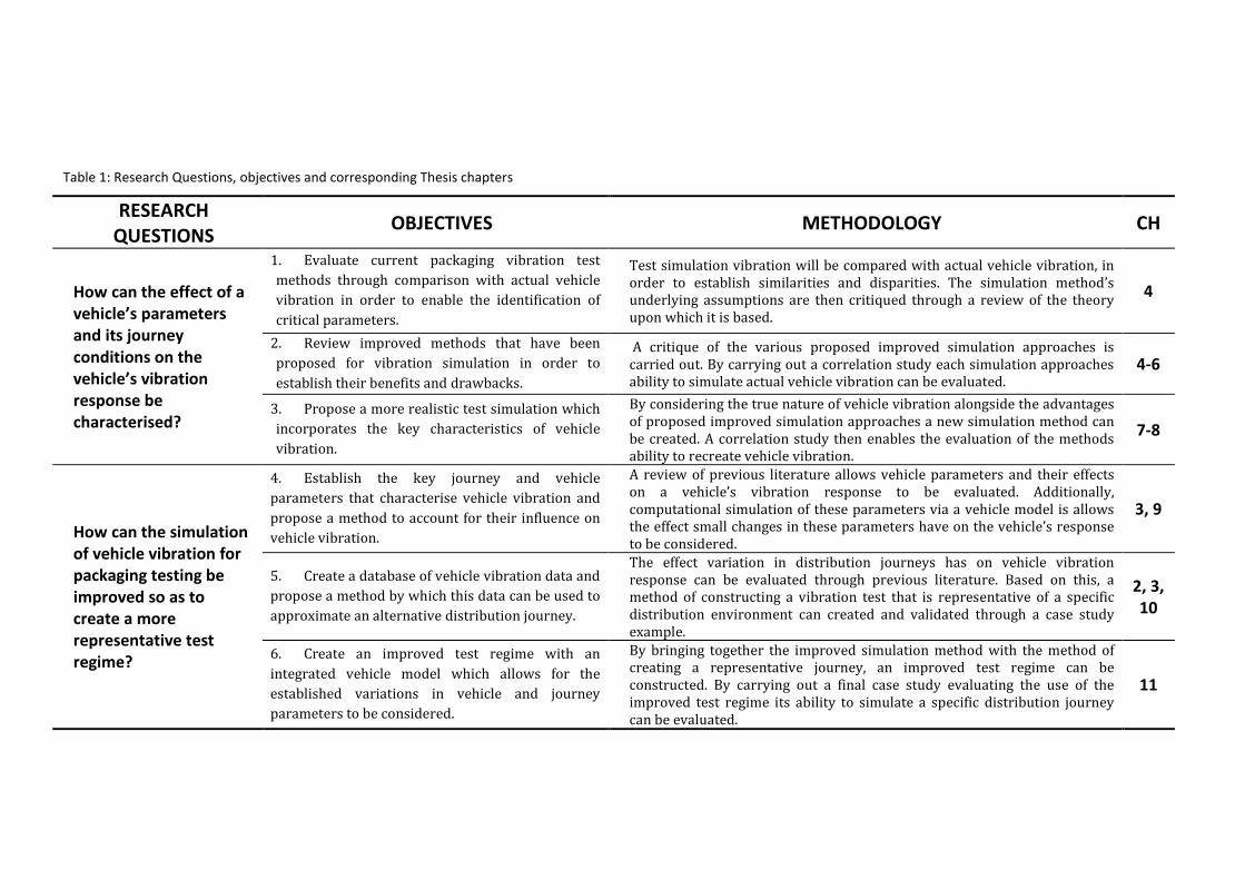
Table 1: Research Questions, objectives and corresponding Thesis chapters
RESEARCH
QUESTIONS OBJECTIVES METHODOLOGY CH
How can the effect of a
vehicle’s parameters
and its journey
conditions on the
vehicle’s vibration
response be
characterised?
1. Evaluate current packaging vibration test
methods through comparison with actual vehicle
vibration in order to enable the identification of
critical parameters.
Test simulation vibration will be compared with actual vehicle vibration, in order to establish similarities and disparities. The simulation method’s underlying assumptions are then critiqued through a review of the theory upon which it is based.
4
2. Review improved methods that have been
proposed for vibration simulation in order to
establish their benefits and drawbacks.
A critique of the various proposed improved simulation approaches is carried out. By carrying out a correlation study each simulation approaches ability to simulate actual vehicle vibration can be evaluated.
4-6
3. Propose a more realistic test simulation which
incorporates the key characteristics of vehicle
vibration.
By considering the true nature of vehicle vibration alongside the advantages of proposed improved simulation approaches a new simulation method can be created. A correlation study then enables the evaluation of the methods ability to recreate vehicle vibration.
7-8
How can the simulation
of vehicle vibration for
packaging testing be
improved so as to
create a more
representative test
regime?
4. Establish the key journey and vehicle
parameters that characterise vehicle vibration and
propose a method to account for their influence on
vehicle vibration.
A review of previous literature allows vehicle parameters and their effects on a vehicle’s vibration response to be evaluated. Additionally, computational simulation of these parameters via a vehicle model is allows the effect small changes in these parameters have on the vehicle’s response to be considered.
3, 9
5. Create a database of vehicle vibration data and
propose a method by which this data can be used to
approximate an alternative distribution journey.
The effect variation in distribution journeys has on vehicle vibration response can be evaluated through previous literature. Based on this, a method of constructing a vibration test that is representative of a specific distribution environment can created and validated through a case study example.
2, 3,
10
6. Create an improved test regime with an
integrated vehicle model which allows for the
established variations in vehicle and journey
parameters to be considered.
By bringing together the improved simulation method with the method of creating a representative journey, an improved test regime can be constructed. By carrying out a final case study evaluating the use of the improved test regime its ability to simulate a specific distribution journey can be evaluated.
11

15
1.4 Research Methodology/Approach
The methodology adopted in this Thesis included an extensive critiquing of both:
the established method of simulating vibration, set out in the current distribution
packaging testing standards; and, proposed improved approaches; through
empirical testing, establishing limitations and benefits of each method. This has
then been used to set the requirements for a new approach. The new approach is
then developed theoretically and verified through a case study.
In addition to this, an evaluation of distribution vehicle vibration, considering
both the vehicle and the journey is carried out, identifying the critical parameters
that shape the vehicle’s response. Using this information an improved method for
building representative simulations is developed. By combining this with the
improved simulation method a new improved test regime is presented. A final
case study is then used to validate this improved test regime.
1.5 Structure of the Thesis
In the first part of Chapter 2 the area of packaging is examined, including its
purpose, classification, the materials used in packaging and the theory behind the
packaging design process. The second part then details the process of distribution
and the distribution chain, highlighting potential hazards and indicating the need
for appropriate packaging solutions. With the need for packaging testing
emphasized, distribution packaging testing is then discussed. Included in this is
an overview of the complete testing cycle within current testing standards.
Chapter 3 focuses on the particular hazard of vehicle vibration. The nature of
vehicle vibration is described as well as its key characteristics. Following this, an
in-depth review of how a vehicle’s vibration response is defined by its parameters
such as speed, suspension, and mass is conducted.

16
An in-depth critique of the current method for vibration testing of distribution
packaging is provided in Chapter 4, followed by a review of proposed improved
simulation methods, including advantages and disadvantages of each method.
Alternatives are considered, including time-frequency analysis tools and multiple
degrees of freedom testing.
In Chapter 5 a case study, that uses the damage mechanism of scuffing to evaluate
each simulation methods’ ability to recreate vehicle vibration, is presented in
order to establish the most appropriate strategy.
Chapter 6 contains a review of the use of multiple degrees of freedom (MDOF)
simulation, previous studies are discussed and a case study evaluating the use of
MDOF compared with single degree of freedom testing is presented.
The use of time-frequency analysis techniques in place of Fourier analysis is
considered in Chapter 7. The advantages of each technique are then discussed.
Following the review of the current method and proposed improved simulation
approaches, Chapter 8 includes a new technique for vibration testing - Wavelet
decomposition. Here a detailed description of the proposed improved simulation
technique is given. An example application is then presented. A case study
evaluating the appropriateness of the Wavelet decomposition method is then
presented. Here a correlation study using the damage mechanism of scuffing is
carried out and the results are compared with those presented in Chapter 5 .
Chapter 9 considers the vehicle’s parameters that affect the shape of its vibration
response. The use of computational vehicle modelling to simulate a given
distribution vehicle’s vibration response from a road profile, is then presented,
along with an inverse vehicle model for predicting road roughness from vehicle
vibration. A sensitivity analysis on vehicle parameters is carried out and the
limitations of using the model are then considered.
Chapter 10 considers Research Question 2 and deals with the variation in journey
parameters. Following this, a method of decomposing a distribution journey and

17
constructing an equivalent simulation journey based on historical vibration data
stored is presented, leading to the proposition of a journey database.
In Chapter 11 the journey database and the wavelet decomposition method are
combined to create the improved test regime. A case study is then used to
demonstrate the appropriateness of the test regime.
A discussion and conclusions are then presented in Chapter 12 and areas of future
work are highlighted.

18
2 DISTRIBUTION AND PACKAGING
Packaging is fundamental to distribution. It has been a key facilitator in the global
distribution of goods. Through advances in packaging materials it has allowed for
extended distribution times and successful distribution through varying climatic
and physical conditions. The processes of packaging design are complex, so as to
meet several main requirements relating to: ergonomics, logistics, sustainability,
safety and marketing (Azzi et al, 2012). Furthermore, there are three different
categories of packaging: primary; secondary; and, tertiary; each of which fulfils a
different role in the distribution chain and can be manufactured from one of four
main packaging materials: glass; metal; plastic; and, cardboard.
The logistical requirements of packaging are there to ensure that the needs of the
complex process of distribution are met. This can consist of numerous stages and
hazards, all of which must be considered alongside the properties of the product
during the design process.
The requirements and common forms of packaging, the distribution cycle in the
context of the food and drink sector and the possible hazards throughout
distribution are discussed.
2.1 The Purpose of Packaging
Packaging design is a complex process that must account for the multiple needs of
the product, distributor, retailer and customer. Azzi et al (2012) identified five
main categories, the needs of which must be considered in order to create a
successful packaging solution. These categories include: ergonomics, logistics,
sustainability, safety and marketing. These overlap and are governed by various
legislation and standards. Consequently, this means that all categories must be
dealt with collectively during packaging design in order to achieve an appropriate
design solution.

19
2.1.1 Ergonomics
IEA (2003) define ergonomics as: ‘the scientific discipline concerned with the
understanding of the interactions among humans and other elements of a system,
and the profession that applies theory, principles, data, and methods to design in
order to optimize human well-being and overall system performance’.
In the distribution of goods there are many stages that include handling or lifting.
As a consequence, for health and safety and an efficient distribution system, the
ergonomics of the process must be considered. Aspects of packaging which affect
ergonomics during distribution, include weight, dimensions and material (Azzi et
al, 2012). International standards exists which impose limitations and guidelines
regarding lifting and carrying, pushing and pulling and handling of low loads at
high frequency. These include ISO 11228 parts 1-3 (ISO, 2009a; ISO, 2009b; ISO,
2009c).
The ergonomics of packaging also have to be considered in terms of the consumer.
In the UK 67,000 people visit hospital for a packaging related injury each year
(Winder et al, 2002). Many injuries occur whilst trying to open packaging. Much
research into the ‘openability’ of packaging has been carried out (Yoxall et al, 2006;
Voorbij and Steenbekkers 2002; Winder et al, 2002). Consideration for aspects
such as ‘openability’, the ability to grip the packaging and the packaged product’s
weight and dimensions, must be considered to ensure an ergonomic packaging
solution.
2.1.2 Logistics
Logistics apply to: ‘...the process of planning, implementing, and controlling the
efficient, effective flow and storage of goods, services and related information, from
the point of origin to the point of consumption, for the purpose of conforming to
customer requirements’ (CLM, 1998).
Logistics are concerned with the transportation, handling, storage and processing
of products from the manufacturer to the point of sale. A product’s packaging can

20
have a direct effect on logistical process efficiency and/or effectiveness. Therefore,
consideration of packaged product shape and size must be made to ensure efficient
use of distribution space.
Packaging must also meet the requirements of the distribution environment,
ensuring it offers the product adequate protection from hazards during
transportation and storage. Unitization is often used to help facilitate the logistical
process, allowing multiple packaged products to be transported and stored at once
so as to reduce handling (Rushton et al, 2010).
2.1.3 Sustainability
Sustainability involves: ‘meeting the needs of the present without compromising
the ability of future generations to meet their own needs’ (Brundtland, 1987)
Sustainability is often divided into three areas (Carter, 2008):
• Environmental - relating to material usage and waste.
• Social - how people interact with the packaging.
• Economic - the financial cost of packaging in terms of material, waste and
the logistical process.
In short, for a packaging solution to be sustainable it must use minimal material
that: is reusable or recyclable; meets the needs of the customer; and, helps
distribution in order to minimise financial costs.
Environmental
Of the three areas, environmental sustainability is the most publicly discussed,
with packaging being considered a major source of pollution in Europe (Bech-
Larsen, 1996). UK market research found that 74% of people interviewed believed
that companies should invest more in sustainable packaging (Mintel, 2012). This
growing public awareness along with a need to reduce packaging waste and a

21
greater increase in knowledge on the subject of sustainability, has led to the
introduction of directives and regulations including:
• Packaging and Packaging Waste Directive 94/62/EC (EPC, 1994)
Introduced by the European Commission in 1994, the directive endeavours to:
keep packaging volume and weight to a minimum while maintaining levels of
product safety, hygiene and acceptance; allow maximum possible reuse or
recovery of packaging; and, minimise the amount of noxious or hazardous
substances from packaging getting into emissions, ash or leachate from
incineration or landfill.
• Courtauld Commitment Phase1 and 2 (WRAP, 2005; WRAP, 2010)
The Courtauld Commitment was created to support the UK policy goal of a 'zero
waste economy' and to help towards the Climate Change Act objective to reduce
greenhouse gas emissions by 34% by 2020 and 80% by 2050. The major UK
supermarkets and some UK producers committed to Phase One of the agreement
in 2005 with the aim of designing out packaging waste growth by 2008, deliver
absolute reductions in packaging waste by 2010 and reducing food waste to
155,000 tonnes by March 2010.
As a result of these regulations there is a greater emphasis on packaging and waste
reduction. Therefore when designing a packaging solution its lifecycle needs to be
considered from manufacture to end use i.e. whether the packaging is reused, the
material is recycled, or, if it becomes waste, whether it goes to compost, landfill or
incineration. These options are now discussed.
• Reuse or return - in some cases the packaging used is in a condition where it
can be reused e.g. carrier bags can be reused by the customer or home
delivery plastic totes can be sent back for reuse. A specific example of
reusable packaging is fibreboard trays used to deliver products by
Riverford Organic (Riverford, 2012). One issue with this approach is that,
the reuse of the carrier bags or the return of the fibreboard boxes is the
customer’s responsibility and therefore much of this packaging is wasted.

22
• Recycle – for items such as glass and aluminium, recycling is considered the
best option. Recycling the material has major energy saving benefits when
compared with the processing of virgin or new material. It was stated by
DEFRA that in 2008 the UK recycled almost two-thirds of all packaging
amounting to 6.6 million tonnes. Within the EU-15 the amount of packaging
waste recycled increased from 46% to 62% between 1997 and 2008
(EUROSTAT, 2008).
• Compost – for materials that are biodegradable compost is the preferred
option rather than sending the waste to landfill. This is also the preferred
option for wasted food items such as fresh fruit and vegetables.
• Landfill – for the EU-15, between 1997 and 2008 the amount of packaging
waste that was sent to landfill decreased significantly from 48% to 29%
(EUROSTAT, 2008).
• Incineration – for energy recovery and generation has become slightly more
popular for the European packaging waste industry. In 1997 only 7% of the
EU-15 packaging waste was incinerated compared with 9% in 2011
(EUROSTAT, 2008).
Social
Social sustainability aims to ‘promotion a democratic, socially inclusive, cohesive,
healthy, safe and just society with respect for fundamental rights and cultural
diversity that creates equal opportunities and combats discrimination in all its
forms’, EUROPEN (2009).
Social sustainability relates to social well-being and the interaction of people with
packaging. In terms of packaging this can cover a multitude of areas including:
• conditions for workers producing, handling and distributing packaging
• protecting public health through protection from hazardous products and
product preservation

23
• preservation of the environment for people through reduced product waste
and the use of environmentally friendly packaging.
Economical
A good packaging design not only means that a product is well protected, but
additionally that it will facilitate efficient and economical distribution. Over
packaging leads to greater material costs, distribution weight and space, which in
turn leads to the use of more fuel and larger or additional vehicles. There are many
costs associated with distribution (Coles and Kirwan, 2011):
• Transport and storage – the size and weight of packaged products
ultimately affects the storage and transport requirements and hence the
cost. Larger items require more space for storage and larger and/or a
greater number of transport vehicles. Additionally, the heavier the load the
greater is the fuel consumption of a vehicle.
• Handling – handling costs are dependent on the unit load - the greater and
heavier the load the greater the cost.
• Inventory control – the packaged products need to be easily identifiable
thereby reducing the length of time the inventory takes.
• Customer service – the better the packaging protects the product, the better
its condition when it reaches the customer leading to a higher level of
customer satisfaction, more repeat business and less returns.
• Environmental impact – the costs associated with the materials used with
regards to manufacturing, preparation for reuse and disposal charges.
Each of these costs needs to be considered in order to create an economically
sustainable packaging solution.

24
2.1.4 Safety
Product safety and protection in terms of chemical, mechanical and biological
hazards and risks has, historically, been the key consideration in the packaging
design process (Hellstrom and Saghir, 2007). The process of distribution can be
long with multiple stages that can include a variety of transport modes,
geographical locations and varying climatic and physical conditions. It is critical
that packaging is designed to protect the product from hazards associated with
these conditions.
The food and drink industry is an area in which the benefit of packaging is
especially evident. Each year 40% of the UK’s food comes from imports, the
majority of which are fresh goods such as fruit, vegetables and meat (Office, 2008).
The delicate nature of these products makes them prone to distribution damage,
the likelihood of which is increased due to extended distribution journeys.
2.2 Marketing
For most products, primary packaging is an important marketing and promotional
tool for the product and the brand. It has been referred to as ‘the salesman on the
shelf’ (Pilditch, 1972). Today, with so much choice, a brand must ensure
prominence to the customer. In some cases the packaging is so critical that it
becomes part of the product. For example, WPO (2008) states that 48% of the
product cost for cola soft drink is in the packaging as it plays a key role in product
and brand identification. Packaging design is also important to consumers. A
survey revealed that 73% of those interviewed rely on packaging to help them
select products (Wells et al, 2007).
Meyers and Lubliner (1998) suggest that in order for a packaging solution to be a
successful marketing tool it must:
• make the product stand out among competitors

25
• identify the product and the brand
• make the product appealing
• communicate product attributes and information
• identify product specific factors such as varieties, flavours, sizes, etc
• enhance the product making it ergonomically appealing.
2.3 Categories of Packaging
In order to meet its numerous requirements, packaging is typically formed of
several layers, each of which serves a specific purpose. The types of packaging can
be divided into three categories: primary; secondary; or, tertiary. The latter two
form the distribution packaging. Hellstrom and Saghir (2007) provide an
illustrated explanation of distribution packaging and this is shown in Figure 6.
Figure 6: Example primary, secondary and tertiary packaging (Hellstrom and Saghir, 2007)

26
Here the primary packaging consists of a single container, which is then shrink-
wrapped in a fibreboard tray of six to form the secondary packaging. This is then
shrink-wrapped and palletised to form the tertiary packaging. The definition of
each is now given.
2.3.1 Primary Packaging
Primary packaging is that which is in direct contact with the product (Hellstrom
and Saghir, 2007). In Figure 7 examples of primary packaging and the materials
used are given.
Figure 7: Examples of primary packaging
Primary packaging forms a barrier between the product and any hazards in the
external environment (Levy, 1999). In the case of perishable goods, such as those

27
illustrated in Figure 7, this barrier is essential in preserving the product and
preventing degradation. This helps maintain the product’s integrity, quality and
safety, resulting in minimal product loss during the distribution process which can
take several weeks (Boonruang et al, 2012). Although the primary packaging
requires certain protective capabilities, for most products it is a major marketing
tool. Examples of primary packaging materials and their properties are given in
Table 2. For each an example product is given, the packaging type and material are
given along with its properties and reasons for use.
Table 2: Primary packaging examples
PRODUCT PACKAGING PROPERTIES
Wine bottle Glass bottle Chemically inert therefore it doesn’t react with the product.
Impermeable to gases, preventing oxidation. It is strong, durable
and transparent allowing the product to be well protected and
visible to the customer. Promotes an image of quality for the
product which is pleasing to the customer.
Coca-cola©
can
Aluminium Light weight. Impermeable to moisture, gas and light, preventing
damage and preserving the product. Allows for pressurisation,
preventing the product from going flat. Highly recyclable.
Box of
chocolates
Cardboard and
plastic (inner
tray)
Stiff, giving the packaging a rigid structure. Printable surface
enabling colourful packaging. Low cost packaging solution.
Versatile, therefore easy to form in to complex shapes and
structures. The plastic inner tray adds to the rigidity of the
package, it also prevents chocolates from damage by separating
and protecting them.
Apple four
pack
Plastic shrink-
wrapped
Carton board
tray
Protects the product from pests and moisture. Provides
regimented way of product stacking and storage which protects
products from surrounding products, preventing inter product
damage.
Packaged
meat
Plastic film Provides high shrinkage allowing it to collapse around product
shape. Excellent protective barrier properties preventing oxygen
and moisture damage. Extends product shelf life.
2.3.2 Distribution Packaging
Distribution packaging, sometimes referred to as logistic or transport packaging, is
used to preserve and protect products in distribution. Included in this category
are: shipping containers; interior protective packaging; and, any unitizing
materials (Marsh, 1997).

28
a. Secondary Packaging
The secondary packaging is a protective packaging that encases and unitizes the
primary packaged product. It helps to ease product handling, and maintain quality
and integrity of the primary packaged product by protecting it from both the
distribution environment and possible interactions with other products (Levy,
1999). The most common type of secondary packaging is the corrugated paper
board boxing, its quality and grade is dependent on the protection required.
Additional product protection is provided by: liners; flutes; and, cushioning
materials. These not only add additional protection during distribution, but also
give additional compressive strength, giving structural strength during stacking
and unitization (Hanlon et al, 1998). An illustrated example of secondary
packaging is given in Figure 8. The product being packaged is wine, the primary
packaging is the glass bottle, and the secondary packaging consists of a corrugated
paperboard box with internal flutes which prevent products from interacting with
each other, and provide additional structural strength enabling the stacking of
boxes.
Figure 8: Example of secondary packaging for wine bottles
In some cases, the secondary packaging forms part of the retail packaging. An
example of this is food items that are unitized in ‘shelf ready’ or ‘display ready’
packaging. Examples of which are given in Figure 9. In this case, whilst providing
protection to the primary packaged product and facilitating distribution, the

29
secondary packaging must also be preserved so that it is presentable for in store
display.
Figure 9: Examples of secondary packaging (a) Display ready packaging (b) Shelf ready packaging
(http://www.packaging-int.com)
Further types of secondary packaging include: shrink-wrapped trays used to
unitize packaged products and ease handling for the retailer; and, corrugated
board boxes which hold several items but do not form part of the sales packaging,
e.g. box used to hold six/twelve wine bottles.
b. Tertiary Packaging
Tertiary packaging eases product handling and transportation by unitizing
secondary packaged products, protecting them from transport and handling
hazards and adverse weather conditions (Ek et al, 2009). By the time the product
reaches the point of sale the majority of tertiary packaging has been removed,
consequently it tends not to form part of the sales or marketing strategy. In order
to help distribution, tertiary packaging can contain information regarding the
product, its point of origin or destination.
Typical forms of tertiary packaging include (Rushton et al, 2010):
• Pallets – where the packaged products are stored uniformly on top of the
pallet and are shrink-wrapped to give structural stability. Pallets allow the
(a) (b)

30
use of forklifts for mechanical handling without risking damage to the
product.
• Cage and box pallets – made of steel or plastic with high mesh sides to
contain the packaged products.
• Roll-cages - made from steel they consist of a mesh cage with shelves inside
to stack packaged products. These are often used during retail distribution
as they allow for mixed loads to be safely stored.
Figure 10: Examples of tertiary packaging
2.4 Packaging Materials and Their Uses
Material selection for packaging depends on the product need. This includes:
protection; preservation; presentation and decoration; and, economics (Twede and
Goddard, 1998). The percentage of packaging materials used by consumption for
the world and the UK is given in Figure 4 (a) and (b), respectively.

31
Figure 11:(a) World packaging consumption by material, 2003 (WPO, 2008) (b) UK Food primary
packaging by material, 2011 (Mintel, 2012)
For distribution packaging paper and board, and plastics are most commonly used.
These materials are now discussed with respect to their protective capabilities and
typical use.
2.4.1 Paper and Board
Paper and board materials are the most commonly used in packaging holding 39%
market share, with corrugated fibreboard box shipping containers forming 40% of
this (Twede and Goddard, 1998). Their popularity is due to rigidity, stacking
strength and ease of storage and distribution. Consequently they provide good
product protection. There is also the added benefit of its recyclability, though
strength degrades when recycled. There are several forms of paper packaging each
designed to have specific properties such as high strength or oil/water resistance
(Twede and Goddard, 1998).
Paperboard is less commonly used in primary food packaging, accounting for only
13%. Its poor barrier properties mean it is not suitable for use to protect
perishable goods from deterioration over the, sometimes, long duration
distribution cycles. It is more frequently used in dry food packaging prior to which
it is often treated in some way to improve its properties i.e. waxed, coated or
laminated (Marsh and Bugusu, 2007). Other forms of wood based packaging used
(a) (b)
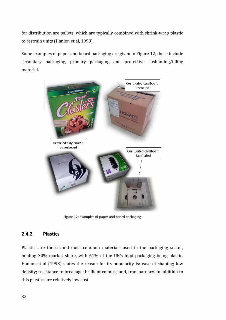
32
for distribution are pallets, which are typically combined with shrink-wrap plastic
to restrain units (Hanlon et al, 1998).
Some examples of paper and board packaging are given in Figure 12, these include
secondary packaging, primary packaging and protective cushioning/filling
material.
Figure 12: Examples of paper and board packaging
2.4.2 Plastics
Plastics are the second most common materials used in the packaging sector,
holding 30% market share, with 61% of the UK’s food packaging being plastic.
Hanlon et al (1998) states the reason for its popularity is: ease of shaping; low
density; resistance to breakage; brilliant colours; and, transparency. In addition to
this plastics are relatively low cost.

33
There are numerous types of plastic available, some widely used plastics are
discussed in (Marsh and Bugusu, 2007), they include:
• Polyethylene terephtalate (PET) – popular for use in food packaging
particularly carbonated beverage bottles. This is because it acts as a good
barrier between the product and external gases and moisture, and it has
good resistance to heat, oils, solvents and acids.
• Polyethylene (PE) – Polyethylene is the most widely used mass produced
plastic. Piringer and Baner (2008) discuss the three common forms of PE:
Low density PE (LDPE), linear LDPE (LLDPE) and high density PE (HDPE).
All of which have good chemical stability, but their mechanical properties
vary:
• LDPE – is used for films or bags due to its soft and flexible nature. It
also offers good transparency. It has a low softening and melting point
which also makes it good for heat sealing.
• LLDPE – is also used for films, but as it stiffer, tougher and has better
barrier properties than LDPE, the film can be made much thinner and
therefore less material is used. It also provides improved transparency
to LDPE.
• HDPE – is much stiffer, harder and stronger than LDPE but is much
less translucent. It is therefore commonly used to for packaging such
as milk bottles, bleach and detergent bottles, or, shampoo bottles. It is
also used in plastic totes or crates for distribution packaging (Figure
13).
• Polypropylene (PP) – is typically used for margarine tubs and
microwavable food trays and containers. It is a tough and flexible plastic
which is reasonably translucent. Additionally, it provides a good moisture
barrier, but poor oxygen barrier. It has a higher softening point than PE.

34
• Polystyrene (PS) – Hard, transparent, high brilliance, it has high resistance
to many chemicals, and good thermal and moisture resistance. It has a high
permeability to gases and is therefore typically used for short shelf life
products such as yoghurt pots or egg cartons. Expanded PS (EPS) is used as
a protective filler packaging on many products, such as electronic items, due
to its cushioning properties, its dimensional stability and its mouldability,
allowing it to be custom made to fit the product easily.
• Polyvinyl Chloride (PVC) – is heavy, stiff, ductile transparent and has
medium strength. It has excellent resistance to chemicals and is typically
used in medical and other non-food packaging, but is sometimes used in
films and bottles for food. It is easy to thermoform and is therefore used for
meat or pharmaceutical blister packaging.
Examples of types of plastic primary packaging were given previously in Figure 7.
Additional examples of plastic distribution packaging are given in Figure 13.
Figure 13: Examples of plastic packaging
2.5 The Packaging Design Process
The design process for packaging is generally accepted to comprise of six steps
(Marsh, 1997):

35
Step 1: Identification of product characteristics
The specification of the product needs to be defined such as its size, weight
and fragility, in order to understand the protective requirements of the
product.
Step 2: Identify marketing and distribution requirements
Details about the product distribution process including frequency, density,
units per container, modes of transport, distribution channels and any specific
handling or storage capabilities required of the packaging, are required.
Step 3: Identify environmental (dynamic and atmospheric) hazards
Evaluation of the distribution environment’s atmospheric and dynamic
conditions and hazards such as temperature and humidity fluctuations and
extremes, transit vibration and shock, handling errors and warehousing and
storage conditions.
Step 4: Consideration of packaging and packaging material
All packaging and unitization methods are considered allowing appropriate
material selection.
Step 5: Packaging specification generated
The specification allows a suitable packaging solution to be designed that
meets the needs of the product, including: the container; interior packaging
and, unitization packaging.
Step 6: Performance testing of packaging solution
An iterative approach is taken to the packaging design process so that the
packaging can be refined and retested until the appropriate level of protection
is obtained. In some cases it can prove more cost effective to redesign the
product rather than the packaging if the cost of damage to the product is

36
significant. Further to this, developing the product packing method to give
maximum protection and stability is also an important part of improving the
packaging design.
Throughout the design process all work should be documented. This includes a
specification detailing the identified requirements of the product-package and all
of the testing carried out.
The performance testing carried out in Step 6 is a vital part of the iterative design
process. By testing packaging prior to distribution, it is possible to ensure the
packaging provides suitable protection for the product, therefore minimising the
risk of product loss or damage during distribution.
2.6 The Distribution Cycle
To fully understand the possible hazards a packaged product will face during
distribution, the cycle of distribution needs to be evaluated from point of
production to the end consumer.
The conditions for distribution will vary depending on product complexity, place of
manufacture and end location. For the majority of products a general distribution
cycle can be followed. Figure 14 illustrates this simplified distribution cycle as
described by (Hellstrom and Saghir, 2007). This process takes the product from
the manufacturer, to one or multiple distribution centres, where the unit
packaging is broken down into the required orders, and then to the retail store and
end consumer.

37
Manufacturers Trans port Trans port
End
Consumer
Filling
Distribution
Centres Retail Outlets
Manufacturers Carriers Wholesalers Carriers Retail outlets
Receiv ing Picking
Warehousing Shipping
Warehousing Receiv ing Replenishing
Re-use/
Recycling
Figure 14: Example of a consumer goods distribution cycle (Hellstrom and Saghir, 2007)
Within Figure 14, the term ‘manufacturers’ represents the multi-facetted
production process. In some cases, such as in the manufacture of processed foods,
a number of products may be involved. These products will have been subjected to
their own process of distribution. In order to simplify the scope of this research,
which is concerned only with distribution and more specifically distribution
packaging, the process of manufacture and the processes prior to manufacture are
not considered.
Today, the fast moving consumer goods (FMCG) industry demands for readily
accessible stock. Therefore primary consolidation centres (PCCs) are used to
warehouse stock in order to ensure that, when needed, the stock at local (regional)
distribution centres (RDCs) can be replenished. This reduces lead times and lowers
distribution costs.
When products are received at the retail stores they are stripped of any additional
packaging and are shelved ready for purchase. Once purchased, products are then
transported to the consumer’s home either by a method of delivery or by the
consumer.
2.6.1 Food and Drink Distribution
The food and drink sector is one of the largest in the FMCG category. It covers a
diverse range of product types with varied requirements, making it a complex and

38
time critical industry in terms of distribution. A typical supermarket distribution
cycle has four key stages. These are:
Stage 1. Producer to the Primary consolidation Centre (PCC)
Within the UK and Europe the majority of distribution is carried out in road
vehicles. In cases where products are imported from greater distances e.g. Asia,
Africa or America, several vehicles and types of transport including air and/or
sea may form this distribution journey.
Stage 2. PCC to the Regional Distribution Centre (RDC)
When stock is required it is transported to the RDC from the PCC using large
road vehicles e.g. semi-trailers.
Stage 3. RDC to the retail store
The RDC replenishes the retail store stock. Again this transport is carried out
using road vehicles. These may be semi trailer vehicles for large stores where
large amounts of multiple products are required or, smaller delivery vehicles for
convenience or small size stores.
Stage4. Retail store to the customer’s home
Once purchased products are transported to the customer’s home via: the
customer using their own vehicle, on public transport or, on foot; or, home
delivery where the retail store delivers the product in delivery vehicles.
Just under half (48%) of food miles occur during Stage 4. This highlights the
significant distance products travel between the retail outlets and the customer’s
home (Steedman and Falk, 2009). The high proportion of food miles during this
final stage, together with the significant reduction in protective packaging, renders
products vulnerable to damage.
The remaining 52% of UK food vehicle miles are due to the transportation of food
through Stages 1, 2 and 3. Of this, approximately 12% are due to transportation of

39
food overseas prior to reaching the UK, 35% are due to transportation of food
within the UK and the remaining 5% of food vehicle miles are from the export of
food from the UK to overseas (Smith et al, 2005). When considering distribution
from the producer to the point of sale, 33% of the food vehicle miles, are overseas.
This overseas distribution accounts for 40% of the UK food supply, with 27% of
the UK’s food coming from EU countries and 13% from other non-EU countries,
including, but not limited to: USA, Brazil, China, India and New Zealand (Barling et
al, 2008). The distribution of the UK food supply source is indicated in Figure 15.
60%27%
13%
UK
EU Countries
Non- EU Countries
Figure 15: percentage of the UK’s food supply by region
The majority of this distribution is carried out by road, with the proportion of
distribution by rail, sea and air being insignificant by comparison. This is because
transport by road is significantly cheaper then air and sea. Unfortunately, the
conditions of road transport vary significantly between countries and therefore
products travelling from different regions will experience different conditions
during distribution.
With these numbers in mind it is clear that in many cases food will not only have
travelled many miles in order to reach the end consumer. It will also have been
subjected to varying transport modes and conditions relating to road types and
quality, and temperature and humidity extremes and fluctuations. How these
conditions vary between distribution journeys is now examined further.

40
2.6.2 Variation in Transport Conditions
Food distribution has been shown to be a global operation. It is therefore apparent
that the distance products travel and the conditions of distribution to which they
are subjected can vary significantly between products. Two key variants in
distribution are the condition of distribution routes and vehicles. For example,
Singh et al (2007) compare vehicle vibration on Indian roads to that presented in
the current testing standards which are based on North American roads. The study
showed that Indian roads produced more severe vibration than that simulated
through the testing standards. The measurements carried out in India were mainly
on paved roads classed as good. In reality, only 50% of Indian roads are paved, and
reportedly only 20% of these are in good condition. In addition, it is reported that
30% of India’s vehicle fleet is over 15 years old (ASIRT, 2004). Therefore, it is
highly likely that the vehicle vibration resulting from a given distribution route and
vehicle will be more intense than that recorded during this study. The variation in
Indian roads to North American roads, on which the current testing standards are
built, is further evident when it is considered that in 2007, 67.4% of North
American roads were paved and 87% of roads were considered to be in a good to
mediocre condition (AASHTO, 2009). Therefore, comparative to Indian roads,
North American roads are in a much better condition and would therefore most
likely provide less harsh distribution conditions.
Other factors which vary between countries are the day and night time
temperatures and humidity fluctuations. Excessive temperature and humidity can
lead to product damage and deterioration if not accounted for when designing the
packaging or selecting the distribution vehicle (Paull, 1999).
The variation in conditions highlighted, illustrates the complexity of distribution
and the numerous considerations that arise. It is therefore important that all
aspects of distribution are considered when choosing or designing appropriate
distribution packaging. This point is stressed by OECD (2002), which states that in
order to create effective and efficient global distribution the diversity in social and
geographical features between countries and their stages of economical

41
development, leading to widely divergent transport systems and operating
structures, needs to be considered.
By considering such aspects of a product’s distribution the requirement of its
packaging can be defined. The typical protective requirements of packaging during
the distribution cycle are now discussed.
2.7 The Requirement of Packaging in the Distribution Chain
Because of the variation in conditions of distribution between geographical
locations, it is essential that to ensure the preservation of product quality during
distribution, the intended distribution cycle and the hazards it may present, are
understood, from the producer to the end consumer. By doing this the
manufacturer, distributor and/or producer can package the product to meet the
needs of distribution (Van Zeebroek et al, 2007). This is true for all products,
whether they are being transported around the world or domestically.
Figure 16 shows the basic distribution cycle with the possible hazards faced at
each stage. Three main areas of distribution are considered, namely: packing and
unpacking; warehousing; and, transportation. The hazard groups identified for
these areas are highlighted in red, with some of the possible hazards then labelled
in green.

42
Fig
ure
16
: T
he
dis
trib
uti
on
cy
cle
an
d i
ts p
oss
ible
ha
zard
s

43
The damage caused by hazards during any one or more of these three stages can
manifest itself through product deterioration externally or internally. Some
forms of damage are described in Table 3 and some examples of the forms of
damage are illustrated in Figure 17.
Table 3: Examples of possible forms of product damage
CATEGORY HAZARD DAMAGE
Vibration
and shock
Fatigue Loss of structural integrity
Impacts
(product on
product and
product on
vehicle)
Cosmetic and product damage such as:
Bruising – reduce quality of fruit and vegetables, accelerate
deterioration
Rupturing – leading to product leakage
Scuffing – ink transfer or damage to products
packaging/product
Gas build up – from constantly shaking product i.e. in a
bottle of carbonated drink
Resonance
Loosen components – excessive vibration could cause
electrical wires to disconnect
Extravagate product damage – excessive vibration could
lead to fatigue damage in the product i.e. additional
bruising
Mishandling
Dropping
Impact damage could lead to cosmetic damage of bruising,
denting, rupturing of packaging which could itself cause
product deterioration or leakages
Forklift
damage
Piercing of external packaging compromising packaging’s
integrity
Piercing of products packaging leading to leakages
Bruising of products through impact
Over
stacking Compression
Lead to cosmetic damage to packaging through
compression which could also cause a loss of the
packaging’s structural integrity
Climatic
fluctuations
Excessive
temperatures
Overheating – cause product to melt or damage the
chemical makeup of the product
High temperatures – accelerate product deterioration
Excessive cold – cause product to freeze and become brittle
or change the chemical makeup of the product
High or low
humidity
High humidity- accelerate product deterioration
Excessive moisture can affect the structural integrity of the
packaging and additionally lead to cosmetic damage
Low humidity – product may dry out damaging the product
i.e. fresh flowers where dry conditions would cause the
flowers to wilt.

44
Figure 17: Examples of types of damage ((a) to (e) taken from (Bai, 2010))
The three main areas of distribution, along with the hazards present within each,
are now discussed.
� Packing/unpacking
Handling – Improper mechanical or manual handling can lead to product
damage and increase its susceptibility to damage through the rest of
the distribution cycle. For example, rough handling or dropping
products can lead to impact damage.
Packing – Incorrect loading of products into packaging can leave it vulnerable
to damage. Additionally, by packing products in mixed loads e.g.
fragile items with heavy items, can further increases the risk of
damage if items are not loaded in an appropriate manner or order.
� Warehousing
Climatic conditions – Subjecting packaged products to harsh climatic conditions
during warehousing can lead to product deterioration and damage,
particularly with fresh produce. Further to this, leaving packaging

45
exposed to adverse weather conditions or high humidity levels can
result in a loss of structural integrity and failure of the packaging.
Stacking – Excessive compressive force or incorrect stacking during
warehousing can lead to product damage and compromise the
structural strength and protective capabilities of packaging.
Handling – Mishandling during stacking can lead to severe product damage,
particularly in cases where products are dropped from great
heights. Mishandling when using forklifts can also lead to other
damage such as piercing or denting.
� Transportation
Vibration and shock – Vehicle vibration during transport, can lead to fatigue
damage of the packaged product, particularly when it is subjected to
lengthy distribution journeys or vibration at a resonant frequency.
Furthermore, shock events caused by road defects or large
displacements in the road surface can cause further product
damage.
Inadequate stacking – Improper loading of items in the distribution vehicle can
lead to excessive shaking, lateral movement or collapsing of stacked
items.
Climatic conditions - Environmental factors such as temperature and humidity
fluctuations can lead to product damage. Changes in temperature
can affect the properties of materials and can cause damage to items
which are temperature sensitive items, such as electronics.
Increased levels of humidity can also lead to mould and bacterial
growth. Moisture can also lead to degradation of fibreboard
packaging such as corrugated boxes, which lose their structural
integrity when wet.

46
It is important to consider the effects of minor damage that occurs during the
distribution process as its cumulative effect may lead to significant damage.
Because of this it is important that all events, including those of low and high
amplitude, should be simulated together in a realistic manner. Testing standards
exist for distribution packaging, which involve subjecting products to these
hazards in order to ensure its protective capabilities.
It is evident that there are many hazards to consider during distribution. The
distribution packaging, and in some cases primary packaging, must meet the
protective requirements of the products. Testing standards provide performance
tests with measured test levels to simulate these hazards to therefore ensure that
a packaging solution provides adequate protection to the product.
2.8 The Testing Standards
Although packaging has many objectives, during distribution its main purpose is
to protect and contain the product. To establish whether a packaging solution is
fit for purpose tests which simulate distribution hazards are carried out. Over the
years, a variety of testing standards have been created which specify test
intensities and testing regimes including both climatic and physical tests.
2.8.1 Temperature and Humidity Testing
There are two forms of temperature and humidity testing, referred to as ‘soak’
and ‘cycle’ tests. Testing is carried out in an isolated test chamber where the
temperature or humidity levels can be closely monitored and controlled.
‘Soak’ tests involve saturating the packaged-product at a particular temperature
or level of humidity and maintaining it for a set period of time. The ‘cycle’ tests
expose the packaged product to repetitive temperature and humidity
fluctuations. This is to simulate the climatic variations which products face during
distribution. ASTM D1469-08 provides test levels that simulate the anticipated

47
rapid changes in conditions. The severity of the tests carried out depends on the
level of assurance required. These tests
evaluate the susceptibility of the packaged
product to moisture or temperature
damage, assessing cosmetic, structural and
chemical damage.
These tests are carried out within either
climatic chambers or cabinets, such as that
shown in Figure 18. These climatic units are
capable of cycling between temperatures as
low as -80oC up to +150oC and relative
humidity from 5 to 95%
Figure 18: Climatic chamber at Smithers Pira
(2012)
2.8.2 Pressure Testing
Pressure/altitude testing is carried out on packages that are transported via
methods that may result in a change in atmospheric pressure. The test schedule
given in ASTM D1469-08 (Section I) covers low pressure (high altitude)
environments, e.g. transportation via aeroplane. ISTA also caters for pressure
testing on the ‘soak’ and ‘cycle’ methods to note the effects of constant low
pressure and varying pressure that may occur when multiple methods of
distribution are required.
2.8.3 Manual and Mechanical Handling Testing
Handling errors during distribution can cause substantial damage to a packaged
product, ISTA (2006) states that single containers, small packages and any
shipping containers that are manually handled up to a weight of 200 lb should be
tested for manual handling hazards. This involves subjecting the packaged-

48
product to drop tests at specified heights using different orientations, assessing
each face and edge for vulnerability to damage.
Mechanical handling tests are only carried out when mechanical handling is the
only anticipated method of handling. These tests are intended for large and heavy
shipping units, and unitized loads.
Both the mechanical and manual handling drop heights vary depending on the
level of assurance required and the weight of the package, the heavier the
package the lower the drop height. For example, in ISTA (2006) for packaging
with a mass less than 9.1 kg drop heights range from 229-610 mm, whilst for
packages with a mass between 45.4 kg and 90.7 kg, drop heights range from 104-
254 mm.
Drop and impact tests are carried out on either free fall drop machines or
mechanical impact machines, as required. Examples of both of these pieces of
equipment are given in Figure 19.
Figure 19: Free fall drop machine (a) and horizontal impact machine (b) at Smithers Pira (2012)
(a) (b)

49
2.8.4 Compression Testing
During warehouse storage packaged products are subjected to compression
loads. Both ASTM and ISTA have test schedules which simulate the loading a
package may suffer during storage. Compression tests include both ‘apply and
release’ and ‘apply and hold’ regimes. ISTA (2010) calculates the force applied
during testing.
Force (N) = Wt * (S-1) * F * 9.8 * 1.4 (1)
This is based on the weight (Wt) of the package, the total number of packaged
products in the stack (S), 9.8 is
representative of g and the duration for
which the package is stacked, (compensation
factor, F). For example, if the package is
stacked for longer than 48 hours then F is
equal to 3.
An example of a compression testing
machine in given in Figure 20, where a
guided steel plate is lowered on to the test
specimen and applies the specified load.
Figure 20: Compression testing machine at
Smithers Pira (2012)
2.8.5 Vibration Testing
There are two methods of vibration testing specified in the various standards. The
simplest is sinusoidal testing, referred to as the ‘resonance search and dwell’
method in ASTM D-999 and ISO standards. Using a simple sine wave the
frequency range of interest (from 3 to 100 Hz) is swept with constant amplitude
typically 0.25g - 0.5g, where g is 9.81 m/s2. During this the resonant frequencies
of the packaged product are identified. The packaged product is then forced to

50
vibrate at, and around, each of its resonant frequencies for a time, typically 15
minutes (Goodwin and Young, 2011). This technique is useful when considering
the response of the packaged product at resonance, but as a vibration test for
simulating vehicle vibration it is an over test due to excessive and unrealistic
vibration at the packaged product’s resonant frequency.
Today it is more common to use an accelerated random vibration test, which
creates a vibration signal based on an average power spectral density (PSD)
spectrum measured from actual vehicle vibration. This test was designed to
create a simulation that better represents the distribution environment. Test
acceleration is carried out based on the theory of fatigue, with the increase in test
amplitude being inversely proportional to the reduction in duration. The two
most common tests include the ASTM and ISTA standards.
There are three types of vibration simulation tables used to carry out vibration
testing. These include electro-hydraulic, which are the most commonly used with
the ISTA and ASTM standards; electro-magnetic, which are capable of high
frequency vibration (>2 kHz) but have a significantly reduced load capacity in
comparison to the electro-hydraulic tables; and, mechanical, this is the most basic
table and is only able to carry out cyclic vibration loading. Each of these tables is
illustrated in Figure 21.
Figure 21: Electro-hydraulic table (a), electro-magnetic table (b) and mechanical table (c) from
Smithers Pira (2012)

51
2.8.6 ASTM Testing Standards
The ASTM standard D4169 details the accelerated random vibration test method.
It presents several simplified PSD spectra for truck, air and rail transport, which
have been calculated using multiple field data and selecting appropriate break
points. The PSD used during testing is dependent on the transport vehicle and the
assurance level required, ranging from i to iii, maximum to minimum assurance.
The PSD spectra provided in D4169 for trucks with leaf spring suspension is
given in Appendix III, Figure 157. Following testing, acceptance of the package
and product is dependent on the selected criteria: product undamaged (i);
packaging intact (ii); or, both the packaging and product undamaged (iii).
The standards specify one spectral shape to be used for each type of vehicle e.g.
all semi trailers with leaf spring suspension. However, they do propose that if
adequate information about the shipping method and its environment is known,
the test should be altered to suit that environment. ASTM D7386 for single parcel
distribution provides a PSD for delivery vehicles.
Additional shock testing of the packaged product is also defined within D4169.
This test applies a shock level vibration to the packaged product for a dwell time
of 60, 40 or 30 minutes depending on the level of assurance. This dwell time is
split between the three axes with 50% of the duration applied along the vertical,
and the remaining 50% split between the lateral and longitudinal direction.
2.8.7 ISTA Testing Standards
The ISTA standards are built up in series test (ISTA, 2012):
Series 1. Integrity Tests –are used to evaluate the toughness and strength of
the packaged product without simulating the distribution
environment.
Series 2. Integrity Plus Tests – combine a mix of integrity tests with at least
one general simulation.

52
Series 3. General Simulation Tests – simulate the distribution environment
based on universal data. They contain standard sets of PSDs, drop
heights and atmospheric conditions.
Series 4. Enhanced Simulation Tests – similar to Series 3, they simulate the
distribution environment but additionally they include at least one
element of focused simulation. This allows the user to integrate test
levels based on a specific distribution environment.
The shape, weight and unitization of different packaged products can vary
significantly and what might be a suitable test for one configuration may not suit
all others. To simulate distribution realistically for different packaging types, each
series contains a number of test standards to suit different configurations. A
number of these packaging configurations and their available testing standards
are given in Table 4.
Table 4: Package types and appropriate ISTA distribution tests (ISTA, 2012)
TEST PACKAGE TYPE DESCRIPTION
1A, 2A,
3A, 4AB Weighing > 150 lb (70 kg)
A single uniform shaped shipment that is less than 150lb (68kg) i.e. corrugated board box. Typically transported in parcel carriers.
1B, 2B,
4AB Weighing > 150 lb (70 kg)
A single uniform shaped a shipment that is greater than 150lb (68kg).
1E, 3E,
4AB Unitized loads
A unit load of the same product i.e. palletised load. Typically transported in Semi Trailers.
2D, 3A,
4AB Considered flat
Specifies specific tests and package faces to carry out tests.
2E, 3A,
4AB Considered elongated
Specifies specific tests and package faces to carry out tests.
2F, 3B,
4AB Less-Than-Truckload (LTL) shipments
Non-uniform shipments i.e. mixed load of packaged-products shipped together
7C Reusable intermediate bulk containers
Plastic containers i.e. for transporting liquids
7A Open reusable transport containers < 60 lb (27 kg) Unitized for shipment on a pallet
Wood/plastic crates or trays that are stacked and unitized
7B Closed reusable transport containers for loads of 150lb (70kg) or less
Wood/plastic closed shipping containers
7D Thermal controlled transport packaging for parcel delivery system shipment
For products which require specific atmospheric conditions i.e. refrigerated or insulated packaging.

53
Each test contains a random vibration test specification similar to ASTM
standards. The random vibration testing in the ISTA standards specify one
spectral shape to be used for each type of vehicle. The PSDs provided in the ISTA
standards for leaf spring and air ride suspension semi-trailers and, over the road
and pick-up and delivery vehicles are provided in Appendix III, Figure 158 and
Figure 159, respectively. By comparison, the shape of the ISTA PSDs are more
detailed than those provided in the ASTM standard, showing more specifically the
definition between the three key resonant frequencies seen in vehicle vibration.
2.9 Concluding Remarks
It is evident that packaging plays a vital part in facilitating product distribution.
The introduction of global distribution has only made its role more important.
Already possessing a vital role, the requirements of packaging are further
expanded through the need for: safety; sustainability; ergonomics; and,
marketing. These requirements of packaging have been established throughout
this Chapter and their fundamental inter-dependency, in order to create a
successful packaging design, has been made apparent.
The importance of these requirements varies depending on the stage of
distribution. During transportation the protective requirement relating to
logistics and safety is critical. A particularly damaging hazard is that of vehicle
vibration and shock during the stages of transportation.
The specific character of vehicle vibration can vary significantly depending on the
type and quality of the roads and the country of travel. With 50% of the UKs food
being imported from overseas it is important to consider the transport routes a
packaged product will take in order to enable consideration of the modes and
conditions of transport. Because of the potential hazards arising during
transportation it can be argued that logistics and safety are most important at
these stages. Without their consideration the successful distribution of the
product would not be possible.

54
For the packaged product to meet its logistical requirements, it is essential that
the packaging provides adequate protection from distribution hazards, whilst
minimising weight and size and the material usage, thereby, enabling fast,
efficient and economic distribution. This logistical role is important for primary
packaging but is most important when considering the secondary and tertiary
distribution packaging. To ensure that the logistical needs of the product are met,
in particular the protective requirement, performance testing which simulates the
distribution environment is used.
The tests provided in the distribution packaging testing standards, provide
specific test conditions to use when evaluating the packaging. The vehicle
vibration tests, which simulate the vibration occurring during transportation, are
based on real data recorded on distribution journeys around North America. With
the aforementioned increase in global distribution and the variation in vehicle
vibration experienced within different regions due to: road type, road quality,
and, the condition of distribution vehicle’s used, the use of a single test (as
provided by the current testing standards) to represent all distribution journeys,
is inadequate. This is particularly true when considering the need for a just right
packaging solution, in order to provide: economic, efficient and sustainable
distribution, whilst ensuring product protection and quality is maintained.
In order to create a more representative vibration test regime, the characteristics
and variations in vehicle vibration need to be assessed. Therefore, Chapter 3
examines vehicle vibration and the aspects of distribution that shape a vehicle’s
vibration response.

55
3 VEHICLE VIBRATION
Vehicle vibration arises from the interaction between the vehicle and the road
surface. The severity of the vehicle’s vibration is dependent on several factors
relating to the system dynamics and the road surface roughness. The combination
of these factors results in a vibration response that is random, non-stationary and
non-Gaussian.
It is widely known that vehicle vibration and shock can cause significant product
damage in packaged product distribution (Lu el al, 2008; Chonhenchob et al,
2008). A vehicle’s vibration response can be greatly affected by small changes in
vehicle parameters or the road input. This sensitivity is difficult to predict. To
understand the sensitivity of a vehicle’s response to changes in vehicle dynamics,
such as: vehicle mass; suspension parameters; and, tyre stiffness, an
understanding of these parameters is required.
A full description of the key characteristics of a vehicle’s vibration response is
given, followed by an examination of the vehicle dynamics that govern it. By
examining these factors the requirements of the vibration testing of packaging
through consideration of the distribution vehicle’s dynamics is developed.
3.1 Terminology
Prior to discussing vehicle vibration, relevant definitions and theory covering
vibration signals and statistical distributions are summarised.
3.1.1 Statistical Properties
The central statistical moments describe the distribution of the variable, x.

56
( )mN
i
irth Xx
Ntmomentm ∑
=
−==1
1)(, (2)
where:
∑=
=N
i
ixN
X
1
1 (3)
is the mean value.
1. Central Mean ( )µ
The first order central statistical moment calculates the central mean of the data
and by definition is equal to zero.
2. Variance ( )2σ
Variance is the second order moment, the square root of which gives the standard
deviation, σ. The variance indicates the size of the spread of the distribution. If a
distribution is Normal and consequently Gaussian, then 68.2% of the distribution
will lie within σ1± , 95.4% within σ2± and 99.7% within σ3± of the mean.
3. Skew ( )γ
Skew is calculated with the third order moment. It is a measure of the symmetry of
the signal where a negative value indicates the distribution is skewed towards the
high values and a positive value indicate the distribution is skewed towards the
lower values. For a Normal (Gaussian) distribution, γ is equal to zero.
4. Kurtosis ( )k
The fourth order moment is kurtosis, which is a measure of the peakedness of a
distribution. The greater the kurtosis the more spiked is the centre of the
distribution. For a distribution centred on zero, this means that a greater portion
of the distribution is focused around the lower values.

57
Dodge (2008) states that ‘...the measures of kurtosis are a part of the measures of
form and characterise an aspect of the form of a given distribution. More precisely,
they characterise the degree of kurtosis of a distribution toward a normal
distribution... To test the kurtosis of a curve we use the coefficient of kurtosis’.
This coefficient of kurtosis is formed from the fourth statistical moment of a
distribution. Typically, and within this Thesis, the standardised kurtosis is used to
define the shape of a signals distribution independent of the unit of measurement.
This is calculated by dividing Equation 2 by the standard deviation raised to the
power four (σ4):
( )4
4
1
1
σ
∑=
−
=
N
i
i XxN
k (4)
A normal (Gaussian) distribution has a standardised kurtosis, k = 3.
3.1.2 Probability Density Function
The Probability Density Function (PDF), P(x), is the derivative of the CDF, F(x). It is
used to calculate the probability that a random variable will take on a specific
value or that it will fall within a particular range of values (Lutes and Sarkani,
2004):
( ) ( )xFdx
dxP =
(5)
Within vibration analysis the PDF is used to illustrate the spread and shape of a
signal’s distribution.
3.1.3 Cumulative Distribution Function
Lutes and Sarkani (2004), state that the cumulative distribution function (CDF) is
probably the most general way to describe the probabilities associated with a

58
given random variable. The CDF, F(x), is a measure of the probability that the
variable x will take on a value equal to or less than X.
∫ ∞−=≤Ρ=
xdPxXxF ξξ )()()( (6)
3.1.4 Gaussian Distribution
A vibration signal is said to have a Gaussian or Normal distribution when its PDF
follows a symmetric, bell shaped curve. The PDF of a vibration signal with a
Gaussian distribution can be defined by:
2
2
1
2
1)(
−−
= σµ
πσ
x
exP (7)
where μ is the mean value of the variable x and σ is its standard deviation.
3.1.5 Calculating the PDF
An example of a PDF is now given for a vehicle vibration signal (which is non-
Gaussian) and a random vibration signal with a Gaussian distribution. Both of
these vibration signals are illustrated in Figure 22.
The PDFs of both signals are then constructed by applying evenly spaced
acceleration level bands (e.g. -5g to 5g with 0.05g increments) to the signal and
finding the number of data points which fall within each band. By then comparing
the number of data points in each acceleration band to the overall number of
points the percentage distribution can be found. The PDFs for both signals are
shown for comparison in Figure 23.

59
0 10 20 30 40 50 60 70 80-1
-0.50
0.51
1.52
2.53
Time (seconds)
Acc
eler
atio
n (
g)
0 10 20 30 40 50 60 70 80-1
-0.50
0.51
1.52
2.53
Time (seconds)
Acc
eler
atio
n (
g)
Gaussian vibration
Vehicle vibration
Figure 22: Example vehicle vibration and the equivalent Gaussian vibration
-1 -0.5 0 0.5 1 1.50
1
2
3
4
5
6
Acceleration (g)
Pro
bab
ilit
y d
ensi
ty f
un
ctio
n(%
)
Vehicle vibration
Gaussian vibration
Figure 23: PDF of the vehicle and Gaussian vibration signals in Figure 22
The variation between the vehicle vibration and the Gaussian vibration can also be
expressed through its kurtosis. For the vehicle vibration k = 10 this is significantly
higher than the k = 3 for the Gaussian vibration. This variation between the two

60
PDFs is made apparent by the sharper peak and wider spread of acceleration levels
in the vehicle vibration’s PDF.
3.1.6 Ensemble Averages
An ensemble refers to a collection of samples x1(t), x2(t), x3(t), ... xn(t) which form a
random process x(t). The random process is formed from a number of samples,
which separately can be considered as independent processes, therefore having
their own statistical values (Newland, 1994).
3.1.7 Stationary Vibration
In the context of vibration the term ‘stationary’ refers to a signal’s ensemble
statistical properties being unchanged by any arbitrary shift along the time axis.
This implies that for any sample of the signal the measured statistical properties
will be unchanged.
When considering the definition of stationary in current research into vehicle
vibration, a signal can be termed stationary the root-mean-square (RMS) of its
acceleration remains constant. The stationarity of the vibration can therefore be
evaluated be measuring the RMS acceleration for fixed length segments of the
signal. If the RMS acceleration is constant the signal is said to be stationary, if the
RMS acceleration varies then the signal is non-stationary (Rouillard and Sek,
2010).
Vehicle vibration is inherently non-stationary due to variations in vehicle speed
and the road roughness (Rouillard and Sek, 2000). This non-stationarity is said to
be exacerbated further, in the long term, because of variations in the vehicle’s
dynamics and payload (Rouillard and Sek, 2001).
In Figure 22, the vehicle vibration is an example of a non-stationary signal and the
Gaussian signal is an example of a stationary signal. The stationarity of the two
signals can be seen in Figure 10 where the distribution of the RMS acceleration of
one second samples of both signals is given. For the vehicle vibration, the RMS

61
acceleration has a distribution spread over the acceleration range 0 – 0.25g, while
the Gaussian signals RMS acceleration distribution is constant at 0.12g.
0
10
20
30
40
50
60
0 0.05 0.1 0.15 0.2 0.25
Occ
urr
ence
(%
)
RMS one second samples (g)
0
10
20
30
40
50
60
70
80
90
100
0.07 0.12 0.17
Occ
urr
ence
(%
)
RMS one second samples (g)
Figure 24: RMS acceleration distribution of one second segments (a) vehicle vibration (b) Gaussian
vibration
3.1.8 Root-Mean-Square
The root-mean-square (RMS) refers to the square root of the mean of the squares
of the values of the variable x:
n
x
RMS
n
i
i∑== 1
2
(8)
The RMS can be used to identify the level of intensity of a vibration signal and as
previously mentioned can be used to identify whether the signal is stationary.
3.1.9 The Fourier Transform
Fourier analysis says that a periodic function may be synthesized as the sum of its
harmonic components (Newland, 1994). This therefore enables the frequency
components within the periodic function to be identified. The continuous Fourier
(a) (b)
RMS one second samples (g) RMS one second samples (g)

62
transform, for the frequency ωk, (X(ωk)), of a signal, x(t), can be calculated using
the Fourier integral (Wong, 2011):
dtetxXtki
k ∫∞∞−
−= ωω )()( (9)
Vibration data acquisition is carried out by measuring acceleration, force or
displacement at equally spaced time intervals over a finite period of time, resulting
in a discrete time series. The frequency coefficients of a discrete time series can be
calculated using the discretised version of the Fourier Transform (DFT). The DFT
is expressed as (Wong, 2011):
∑−
=
−=1
0
)/2(N
r
Nkrirk exX π
(10)
where Xk is the DFT of an input sequence xr, of length N. r is the current sample
being considered (0, 1, 2, ..., N-1) and k is the current frequency component being
considered (0 1, 2, ..., N-1).
The Inverse DFT (IDFT) is given by:
∑−
=
=1
0
)/2(1 N
r
Nkrikr eX
Nx π
(11)
For a time domain signal, x(t), with sample interval Δt, and finite duration NΔt, the
DFT at frequency fk Hz, can be found using the equation:
∑−
=
−=1
0
2)()(
N
r
rtkfirk etxfX
π (12)
where the DFT frequency, fk = k/NΔt Hz, and tr = rΔt.
In frequency analysis the rate at which a signal is sampled sets a limit as to the
maximum frequency that can be detected within that signal, this limitation is
referred to as Shannon sampling theorem (Shiavi, 2007). This means that for a
signal with a sampling frequency, fs = 1/Δt Hz, the highest frequency that can be
detected within that signal is fn = fs/2 Hz, where fn is often referred to as the

63
Nyquist frequency. When analysing a signal for frequencies greater than fn, the
frequency information becomes indistinguishable so that frequencies greater than
fn appear as false low frequencies, this is referred to as aliasing. An example of
aliasing is given in Figure 25. The figure illustrates a sine wave with frequency, f =
8 Hz. This sine wave is then sampled with fs = 10Hz, so that the maximum
frequency that can be detected is fn = 5 Hz, therefore aliasing will occur. Aliasing
will cause the 8 Hz sine wave to be detected as a sine wave with frequency, (f – fs),
hence a sine wave with frequency, f = -2 Hz.
-1
-0.5
0
0.5
1
0 0.2 0.4 0.6 0.8 1
Acc
eler
atio
n (
g)
Time (seconds)
8 Hz Sine wave 8 Hz sine wave sampled at fs = 10 Hz
8 Hz Sine wave identified as -2 Hz sine wave
Figure 25: Example of signal aliasing
The Shannon sampling theorem gives the DFT the inherent property: X(fN-k) = X(fk).
The DFT therefore forms a two-sided spectrum, with positive and negative
frequency values. For analysis purposes, typically, only the one sided spectrum is
required. To create the one sided spectrum, the Fourier spectrum, X(f), must be
truncated after the N/2th value.
To speed up the calculation of the DFT the Fast Fourier Transform (FFT)
computational algorithm is used. This efficiently calculates the DFT of a signal.
While the DFT requires N2 calculations, the FFT requires only Nlog2N calculations,
which significantly reduces the processing time and computational power required
to carry out the DFT (Newland, 1994).

64
3.1.10 Power Spectral Density
The power spectral density (PSD) spectrum ‘...shows how the different frequencies
contribute to the variation in the signal.’ (Shaivi, 2007). It does this by defining the
power content within each frequency band (Δf) of the signal (x(t)) enabling key
frequency components within a signal to be identified. Power is defined as the
acceleration squared (g2), where g = 9.81 m/s2, so that the PSD is g2/Hz.
Shiavi (2007) defines the equation for the PSD in two forms, firstly, as the Fourier
transform of the autocorrelation function:
∫ −= ττπ
π deRfS fti2)(2
1)( (13)
where the autocorrelation function is the cross-correlation of the signal, x(t) with
itself at time lag τ:
τττ dtxtxT
RT
∫ +=0
)()(1
)( (14)
Secondly, as a function of frequency:
NT
fXfXfS
)(*)()(
•= (15)
where, T = 1/Δt, is the sample period, is the sampling frequency, so that the
frequency bandwidth, Δf = 1/NΔt Hz. N is the number of data points within the
signal being analysed (length of the DFT) and X(f) is the Fourier spectrum of
length N.
3.2 The Characteristics of Vehicle Vibration
Excitation of the vehicle as it traverses over a rough road surface results in vehicle
vibration (Rouillard, 2007a; Rouillard and Sek, 2000). In addition to relatively
consistent variations in the road surface roughness, large deviations due to

65
hazards such as potholes or speed bumps are also present. The occurrence and
location of these are random in nature and are difficult to predict. Their presence
can lead to discrete high energy events in the vehicle’s response. The amplitude
and shape of the vehicle’s response is then further dependent on the vehicle’s
speed profile and parameters.
Although for different vehicles the amplitude and shape of the response will vary,
several key characteristics will remain. Firstly, as previously stated, all vehicle
vibration is random, non-stationary and of a non-Gaussian distribution. Secondly,
all vehicle vibration embodies three key resonant frequencies 1 - 5 Hz suspension
resonance, 10 - 15 Hz resonance of the unsprung mass or ‘wheel hop’ and 40 - 55
Hz structural resonance. The exact frequency of each depends on the vehicle’s
parameters (Singh et al, 2008; Rouillard and Sek, 2001).
A more in depth description of the key characteristics of vehicle vibration is now
given.
3.3 The Non-Stationarity of Vehicle Vibration
Vehicle vibration is highly non-stationary due to constant fluctuations in vehicle
speed and road roughness, and, in the long term, because of variations in a
vehicle’s dynamics and payload (Rouillard and Sek, 2000; Nei et al, 2008; Rouillard
and Sek, 2001). These changes result in vibration with a continually varying RMS
acceleration, as illustrated in Figure 24. The three main sources attributed to the
non-stationarity of vehicle vibration are:
• Fluctuations in road surface roughness - road surface roughness is random
and non-stationary (Bogsjo, 2006). This means that the severity of the
input due to road roughness will vary with time, ultimately affecting the
amplitude of the vehicle’s vibration response (Rouillard and Sek, 2005).
• Fluctuations in vehicle speed - throughout a journey a vehicle’s speed will
experience large fluctuations due to changes in speed restrictions and

66
smaller fluctuations due to changing acceleration levels. When combined
these result in a time variant vehicle response (Richards, 1990).
• Frequency or spectral non-stationarity - this third type of non-stationarity
arises from structural excitation of the vehicle’s modal frequencies. It is
noted as being rare in road vehicles due to ‘the relatively compliant
suspension systems and slack-free coupling mechanisms’ (Rouillard and Sek,
2005).
3.4 Non-Gaussian Distribution of Vehicle Vibration
The statistical distribution of vehicle vibration acceleration levels has been shown
on many occasions to be non-Gaussian (Otari et al, 2011; Garcia-Romeu-Martinez
and Rouillard, 2011). A combination of consistent variations in the road surface
roughness and large deviations due to road damage, traffic calming, kerbs, etc.,
results in a non-Gaussian road surface roughness, which ultimately results in a
vehicle response that is also non-Gaussian in character (Bruscella et al, 1999;
Bogjso et al, 2012)
When measuring the shape of the acceleration distribution for vehicle vibration,
the value of kurtosis is often used for comparison with the Gaussian. Rouillard and
Sek (2010) found that the kurtosis of vehicle vibration was much higher than the
kurtosis value of 3 which represents a Gaussian distribution (Rouillard, 2007b).
Their work showed the kurtosis varies between 5.5 and 14.7 for different vehicle
types, as shown in Table 5.
The deviation in the vibration distribution from the Gaussian profile tends to
manifests itself as a sharp peak at around zero and long tails. This is due to the
presences of discrete high level shock events and low level vibration (Lu et al,
2008). An equivalent Gaussian signal (meaning a random vibration signal with a
Gaussian distribution, with the same average RMS acceleration and frequency
content as the original vibration signal) would consist of a higher level of constant
vibration but would noticeably be missing the peak acceleration shock events.

67
Table 5: Overall kurtosis for various distribution vibration records (Rouillard and Sek, 2010)
ID VEHICLE TYPE AND LOAD ROUTE TYPE KURTOSIS
MA Utility vehicle (1 tonne capacity)
Load<5% capacity Suburban streets 8.8
MB Prime mover + semi trailer (Air ride susp.)
Load:90% capacity Country roads 9.7
MC Transport van (700 kg capacity)
Load 60% capacity Suburban streets 7.3
MD Transport van (700 kg capacity)
Load: 60% Capacity
Main suburban
highway 10.2
ME Transport van (700 kg capacity)
Load: 60% Capacity Motorway 8.2
MF Prime mover + semi trailer (Leaf spring susp.)
Load: <5% capacity Country roads 14.7
MG Tipper truck (16 tonne capacity, Air ride susp.)
Load: 25% capacity Country roads 5.5
MH Small flat bed truck (1 tonne capacity, leaf
spring susp.) Load: <5% capacity Suburban streets 8.4
MK Sedan car
Load: 1 passenger Suburban streets 12.0
This inherent non-Gaussian nature was also studied by Sek (1996), where the
amplitudes of peak vehicle vibration acceleration levels were compared with the
peak levels of the equivalent Gaussian signal. It was shown that for the vehicle
vibration, 99.7% of acceleration levels fell within the limits +/- 1.25g, whilst for the
equivalent Gaussian signal 99.7% of the data fell within the reduced limits of +/-
0.75g (where g = 9.81 m/s2), hence highlighting further the fundamentally non-
Gaussian nature of vehicle vibration.
It should be noted that within this Thesis vibration has been measured using
acceleration using the unit g = 9.81 m/s2.
3.5 Vehicle Vibration Frequency Response
The major frequencies contributing to the vibration of a vehicle generally fall
below 100 Hz, with the most significant of these below 50 Hz. Frequencies above
50Hz tend to be insignificant in comparison ( Vursavus and Ozguven, 2004; Peleg,
1985). A vehicle’s vibration response is typically measured within the range of 1

68
Hz to 200 or 250 Hz (Chonhenchob et al, 2012; Singh et al, 2006; Lu et al, 2008).
Within this range there are three key resonant frequencies:
1. Body resonance in the suspension system - this lies between 1 - 5 Hz, with
air ride suspension systems typically in the range 1 - 1.5 Hz and leaf spring
suspension systems 4 - 5 Hz (Garcia-Romeu-Martinez et al, 2008).
2. Resonance of the unsprung mass – i.e. the unsuspended part of the vehicle,
is typically in the range 10 - 20 Hz (Singh et al, 2007). Vehicle dynamists
refer to this resonance as ‘wheel hop’ which is typically around 12 Hz.
3. Resonance of the vehicle’s structure - has been found to be up to 100 Hz
(Suciu et al, 2012). More specifically, for semi trailer vehicles, this third
frequency lies between 40 - 55 Hz (Singh et al, 2007).
Changes in vehicle parameters can lead to changes in the vehicle’s resonant
frequencies. For example, the lower the sprung mass of the vehicle the higher the
first natural frequency. By reducing the suspension stiffness or tyre stiffness there
will be a reduction in the corresponding natural frequency (Rajamani, 2012). A
comparison of different vehicle types including: a passenger car (2 tonnes); pickup
truck (2.7 tonnes); two small delivery vans (3.9 tonnes); and, a freightliner (7.3
tonnes); illustrated the variation in vehicle frequency response. The results of the
study are shown in Figure 26.

69
Figure 26: Comparison of PSD’s for the vertical vibration response of different vehicle types
(Chonhenchob et al, 2012)
In Figure 26 the freightliner’s suspension resonant frequency is in the region of 3 -
4 Hz, whilst the suspension resonant frequency of the other smaller vehicles is
around 2 Hz. What is also apparent is the overall variation in the energy content,
with the Honda car having significantly lower energy content than the larger
vehicles.
3.6 Vehicle Vibration’s Multiple Degrees of Freedom (MDOF)
A vehicle’s response is defined by the road input and its parameters. The irregular
and asymmetric nature of these produces a six degree of freedom response at any
point on the vehicle floor. This includes three linear: vertical; longitudinal; and,
lateral; and, three rotational: pitch; roll; and, yaw. These are illustrated in Figure
27. Typically, the vertical vibration of the vehicle contains the most energy and
therefore has the most significant damage potential, this has been corroborated in
PSD (g2/Hz)
Frequency (Hz)

70
a number of studies (Singh et al, 2006; Singh et al, 1992; Singh et al, 2008;
Chonhenchob et al, 2012). Hence, historically, vibration testing of packaging has
been carried out using a single degree of freedom (SDOF) test that represents the
vertical motion of the vehicle floor. A further reason for this is the limitation of
many vibration tables and controllers, which are restricted to single or a partial set
of DOFs. However, multi axes rigs exist and it is thus possible to simulate the full
motion of the vehicle floor, at a point.
Longitudinal, x
Lateral, y
Vertical, z
Roll
Pitch
Yaw
Figure 27: Translational and rotational axis of MDOF response of vehicle floor
In contrast, Bernad et al (2010) argue that there may be a need for MDOF testing.
Bernard et al used operational modal analysis to compare the bending moments of
a stack with the vertical resonances. The study concluded that, as packaging is
primarily designed for compression strength, the effects of the lateral and
longitudinal vibration on the stack may consequently be significant, and lead to
either sliding and/or stack failure.
Singh et al (1992) considered the three translational degrees of freedom. When
comparing the energy of the vibration of each of the three axes it was clear that
below 20 Hz the vertical component was significantly greater than the longitudinal
or lateral. However, above 20 Hz, the energies along each of the axes were similar.
It was also noted that the more heavily laden a truck, the greater the amplitude of
the lateral and longitudinal vibration.
Singh et al (2008) also measured the RMS acceleration values of each of the
translational axis during a Less-Than-Truckload (LTL) shipment, these were

71
0.338g, 0.095g and 0.088g for the vertical, lateral and longitudinal axes,
respectively. This variation in intensity for each translational axis is agreed with by
Bernad et al (2011), where the RMS acceleration values were found to be 0.091g,
0.056g and 0.039g, respectively.
Contrary to the results shown in these studies, which use vibration measured on
North American roads, results from a study measuring vibration on Indian roads
showed that the lateral and longitudinal vibration was of greater significance. Here
the average RMS acceleration values were 0.138g and 0.063g for the lateral and
longitudinal vibration, respectively, and 0.151g for the vertical axis (Singh et al,
2007).
In a similar manner to the linear axes, Bernad et al (2011) also investigated the
rotational axes of vibration. The results showed that the pitch and roll components
of the measured vibration were much greater than the yaw component, with RMS
acceleration values of 0.94, 0.81 and 0.525 rad/s2, respectively. The pitching
motion had a spectral peak at around 2 Hz and both pitch and roll showed a
notable response at approximately 7 Hz. The roll motion showed a high frequency
content above 20 Hz with its peak value at around 36 Hz.
Whilst a vehicle’s vertical vibration may be greater in magnitude than its lateral
and longitudinal vibrations, previous studies have shown that the amplitude of the
latter two can become more significant depending on geographical location.
Although in comparison, vibration in the other axes may appear insignificant, their
combined affect at resonant frequencies could impact on product damage. It is
therefore necessary to evaluate the contribution to damage of the other axes.
3.7 The Factors That Influence Vehicle Vibration
Vehicle vibration results from the complex interaction between the road surface
and the vehicle. Vursavus and Ozguven (2004) determined that the road
roughness; distance travelled; vehicle speed; product packaging; and, vehicle
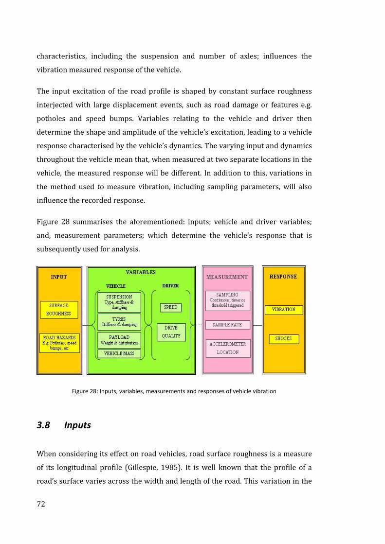
72
characteristics, including the suspension and number of axles; influences the
vibration measured response of the vehicle.
The input excitation of the road profile is shaped by constant surface roughness
interjected with large displacement events, such as road damage or features e.g.
potholes and speed bumps. Variables relating to the vehicle and driver then
determine the shape and amplitude of the vehicle’s excitation, leading to a vehicle
response characterised by the vehicle’s dynamics. The varying input and dynamics
throughout the vehicle mean that, when measured at two separate locations in the
vehicle, the measured response will be different. In addition to this, variations in
the method used to measure vibration, including sampling parameters, will also
influence the recorded response.
Figure 28 summarises the aforementioned: inputs; vehicle and driver variables;
and, measurement parameters; which determine the vehicle’s response that is
subsequently used for analysis.
Figure 28: Inputs, variables, measurements and responses of vehicle vibration
3.8 Inputs
When considering its effect on road vehicles, road surface roughness is a measure
of its longitudinal profile (Gillespie, 1985). It is well known that the profile of a
road’s surface varies across the width and length of the road. This variation in the

73
road profile is further increased by the presence of localized road damage or
hazards in the form of large deviations in the road surface. These are typically
random and rarely cover the width of the road. A combination of the surface
roughness, road damage and hazards are what shape the initial excitation of the
vehicle. Therefore from the outset, the vehicle’s response is random,
unpredictable.
3.8.1 Surface Roughness
It is universally accepted that the overall condition of roads varies significantly
between countries. A review of the percentage of paved roads – roads which have
been covered with a layer of material e.g. concrete, asphalt, bitumen, etc -
highlighted the lack of infrastructure in some of the world’s developing countries,
such as Bolivia and Kenya where only 7.9% and 14.3% of the roads are paved,
respectively (FAO, 2004). Evaluating a country’s road quality by the percentage of
paved roads is not a perfect indication of road quality due to anomalies, for
example Australia. Here the percentage of paved roads is relatively low due to the
size of the country and population distribution. Therefore, the percentage of paved
roads can act as a good indicator of the general conditions of distribution and
highlight the extremes of countries with a severe lack of infrastructure and that
therefore are more likely to provide harsh distribution conditions.
In section 2.6.2 the variation in road conditions in India was compared with that of
North America. Singh et al (2007) showed that in comparison with the PSD given
in the current ISTA standards, the amplitude of the PSD recorded on Indian roads
was 10 - 70 times higher in the frequency range of 1 – 5 Hz. This increased
intensity at the low frequency range will lead to much larger vertical displacement
of the vehicle, than that produced from the standards PSDs. This highlights the
variation in road roughness between countries, with Indian roads having many
more or larger road defects.
The roughness of roads in India was calculated by Ramji et al (2004) using the
spatial PSD, measuring the roads vertical displacement (m) in relation to the road
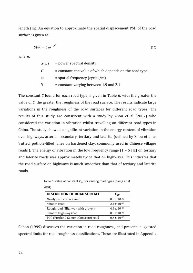
74
length (m). An equation to approximate the spatial displacement PSD of the road
surface is given as:
NCS −= ωω)( (16)
where:
)(ωS = power spectral density
C = constant, the value of which depends on the road type
ω = spatial frequency (cycles/m)
N = constant varying between 1.9 and 2.1
The constant C found for each road type is given in Table 6, with the greater the
value of C, the greater the roughness of the road surface. The results indicate large
variations in the roughness of the road surfaces for different road types. The
results of this study are consistent with a study by Zhou et al (2007) who
considered the variation in vibration whilst travelling on different road types in
China. The study showed a significant variation in the energy content of vibration
over highways, arterial, secondary, tertiary and laterite (defined by Zhou et al as
‘rutted, pothole-filled lanes on hardened clay, commonly used in Chinese villages
roads’). The energy of vibration in the low frequency range (1 – 5 Hz) on tertiary
and laterite roads was approximately twice that on highways. This indicates that
the road surface on highways is much smoother than that of tertiary and laterite
roads.
Table 6: value of constant Csp, for varying road types (Ramji et al,
2004)
DESCRIPTION OF ROAD SURFACE CSP
Newly Laid surface road 0.3 x 10-06
Smooth road 2.4 x 10-06
Rough road (Highway with gravel) 4.4 x 10-06
Smooth Highway road 0.5 x 10-06
PCC (Portland Cement Concrete) road 0.6 x 10-06
Cebon (1999) discusses the variation in road roughness, and presents suggested
spectral limits for road roughness classifications. These are illustrated in Appendix

75
IV, Figure 134. By superimposing a road’s surface profile displacement PSD onto
the limits the roughness of the profile can be evaluated.
3.8.2 Road Hazards
The road construction also has a bearing on the vehicle’s response, in terms of:
paving material; man-made hazards such as traffic calming measures (speed
bumps); kerbs or raised metal joints; and, road damage such as potholes. These
can cause potentially damaging high amplitude shock events, depending upon the
speed at which they are approached. Figure 29 shows the effect hazards have on a
vehicle’s response: (a) shows the response of a home delivery vehicle travelling at
15 mph over a speed bump when a peak acceleration of 2g was recorded and (b)
shows the same vehicle’s response when it mounted a kerb at 15 mph when a peak
acceleration of 0.85g was recorded. Figure 30 shows the related hazards. The
presence of hazards can greatly affect the overall response of the vehicle. It is
therefore evident that when creating a simulation test the condition of roads
throughout the distribution route needs to be taken into consideration.
0 1 2 3 4-2
-1
0
1
2
Time (Seconds)
Acc
eler
atio
n (
g)
0 1 2 3 4-1
-0.5
0
0.5
1
Time (Seconds)
Acc
eler
atio
n (
g)
Figure 29: Vehicle vibration response to (a) Speed bump (b) Pavement kerb

76
Figure 30: (a) Speed bump (b) Pavement kerb
Variation in road roughness also arises from the use of different construction
materials. This variation can be seen in one study where the PSDs determined from
travel on concrete Spanish roads produced much higher spectral peaks and
therefore a higher intensity vibration than the PSDs from travel on asphalt French
roads (Barchi et al, 2002). The difference between the two spectra was evident
with the first spectral peak at around 9 Hz varying from approximately 0.008
(m/s2)2/Hz on Spanish roads to 0.003 (m/s2)2/Hz on French roads. This difference
can also be seen at the second spectral peak at around 20 Hz where the Spanish
road’s peak is approximately 0.15 (m/s2)2/Hz, and, the peak for French roads is
0.11 (m/s2)2/Hz. This shows overall, that the Spanish concrete roads produced a
more severe journey.
Furthermore, another study compared a vehicle’s response on roads constructed,
respectively, of laterite (defined in the study as loose gravel on hardened clay,
commonly used in farm regions), concrete (highway) and asphalt (highway). The
results showed a significant difference in the amount of damage occurring to the
test product. For a 2 tonne truck travelling at 40 km/hr, the average product
damage on Laterite roads was 10%, on concrete 4.7% and on asphalt 2.0%
(Jarimopas et al, 2005). This demonstrates that the road profile of laterite roads is
much harsher than that of concrete or asphalt.
These studies highlight the fact that road surface roughness is not just
characterised by road condition, but rather, a number of factors pertaining to the
road’s construction, material and also additional hazards that can result in large
displacements of the road surface. Therefore, when estimating the intensity and

77
characteristics of vehicle vibration for a given distribution journey, the country of
distribution and the road types travelled on should be considered.
3.9 Variables
Whilst the intensity of the initial input to the vehicle is determined by the roads
travelled, the magnitude and shape of the vehicle’s response to that input is
characterised by the vehicle’s parameters such as the suspension system, tyre
dynamics and vehicle payload. The variations in vehicle parameters and their
effect on a vehicle’s response are now summarised.
3.9.1 Suspension
The suspension system is critical in protecting the vehicle from excessive shock
and vibration loading, which can cause damage and/or fatigue (Garret et al, 2001).
The vehicle’s suspension system has a significant effect on the vehicle’s handling
and ride comfort. Because of this, many distribution vehicle manufacturers build a
vehicle to suit the customer’s requirements. This means that suspension
characteristics can vary not only between vehicle types, but between similar
vehicles depending on their intended load. Any variation in suspension
characteristics will ultimately be seen in the vehicle’s vibration response. There
are three main categories of suspension system: passive, semi-active and active,
these have each been described by Jalili (2002) as:
• Passive
Passive suspension systems consist of a stiffness member (spring) of stiffness
Ks and a fixed rate damper, which dissipates vibration energy, with damping
rate CS. The performance of the passive system varies with frequency, with the
system having a limited frequency range. It therefore has an inherent
compromise on frequency isolation. Because of its fixed rate, the passive
suspension system’s performance is limited particularly when considering

78
broadband frequency range applications. Figure 31(a), illustrates a passive
suspension system within a quarter vehicle model.
• Active
By including an additional feedback controlled actuator, an active suspension
system with adaptable to different driving conditions is created. By measuring
the acceleration of the vehicle’s mass and the unsprung mass, the actuator
force can be controlled so as to minimise the force transferred to the vehicle
floor.
The computation requirements and the additional components of an active
suspension result in an expensive and complex system with high energy
consumption. Figure 31(c), illustrates a passive suspension system within a
quarter vehicle model.
• Semi-active
A Semi-active system bridges the gap between the capabilities, and the
limitations of the passive and the active suspension systems. Like the passive
system, it comprises of a damper and spring element but, in addition, it allows
for variation in its optimal frequency range, although by comparison to the
active system this is relatively limited.
Air ride suspension is a semi active system, whereby the stiffness member
consists of an air spring or hydro pneumatic system. Figure 31(b), illustrates a
passive suspension system within a quarter vehicle model.
In Figure 31, MV is a quarter of the vehicle mass, MT is a quarter of the unsprung
mass, KT is the tyre stiffness, and, x0, x1 and x2 are the vertical displacements of the:
road, unsprung mass and vehicle, respectively.

79
MV
MT
Ks Cs
x1
x2
x0
KT
MV
MT
Ks(t) Cs(t)
x1
x2
x0
KT
MV
MT
Ks Cs
x1
x2
x0
KT
U(t) Controller
Sensor
Sensor
Figure 31: Quarter vehicle model with (a) passive (b) semi-active, and (c) active suspension
The two most common forms of distribution vehicle suspension system, which are
both simulated in the current ASTM and ISTA standards are the passive spring leaf
or semi-active air ride suspension.
3.9.2 Spring-Leaf and Air Ride Suspension
The stiffness of the leaf spring suspension system remains fixed for all load
configurations. Therefore, when designing the suspension system, both the vehicle
mass and its mass when fully laden need to be considered. This limitation means
that the performance of a suspension system that is designed to attain and meet
the requirements of a suitable ride height (distance of the vehicle floor from the
road) for a fully laden vehicle will be greatly diminished. This will lead to a poor
ride quality when the vehicle is part loaded or empty. Additionally, constant
stiffness coupled with varied payload will cause variation in the vehicle’s resonant
frequency. As a way of improving ride quality in distribution vehicles,
manufacturers tend to design the suspension system to meet the requirements of
the load it is intended to carry. This means that suspension systems and their
characteristics not only vary between vehicle manufacturers and models, but also
between the individual vehicles themselves.
Damping within the spring leaf system is provided via either the spring friction
(typically flat leaf springs, with high Coulomb friction) or, through shock
absorbers with either fixed or variable damping depending on the system type

80
(Gillespie, 1985). An example of a leaf spring suspension system is given in Figure
32(b).
Semi-active air ride (air sprung) suspension is the main alternative to the passive
leaf spring system. It consists of a pressurized elastomeric bag, which lifts the
sprung mass of the vehicle. When the vehicle load varies, the pressure in the air
springs also varies so that the correct ride height of the vehicle is maintained.
Because the air spring’s stiffness varies proportionally to the vehicle mass, its
resonant frequency remains constant at all loads. Hydraulic shock absorbers are
used to provide the necessary damping as the air spring’s friction is too low to
satisfy the damping requirement (Gillespie, 1985). An example of a leaf spring
suspension system is given in Figure 32(a).
Air spring Leaf spring
Figure 32: Examples of air ride (a) and leaf spring (b) suspension systems take from (Garcia-Romeu-
Martinez et al, 2008)
The variation in ‘ride quality’ between the two suspension systems can be seen by
comparison of the PSD spectra provided in the current testing standards
(Appendix III: Figure 157, Figure 158 and Figure 159). The first spectral peak of
the air ride semi-trailer PSD is 0.009 g2/Hz, and it is 0.018 g2/Hz, for the steel
(a) (b)
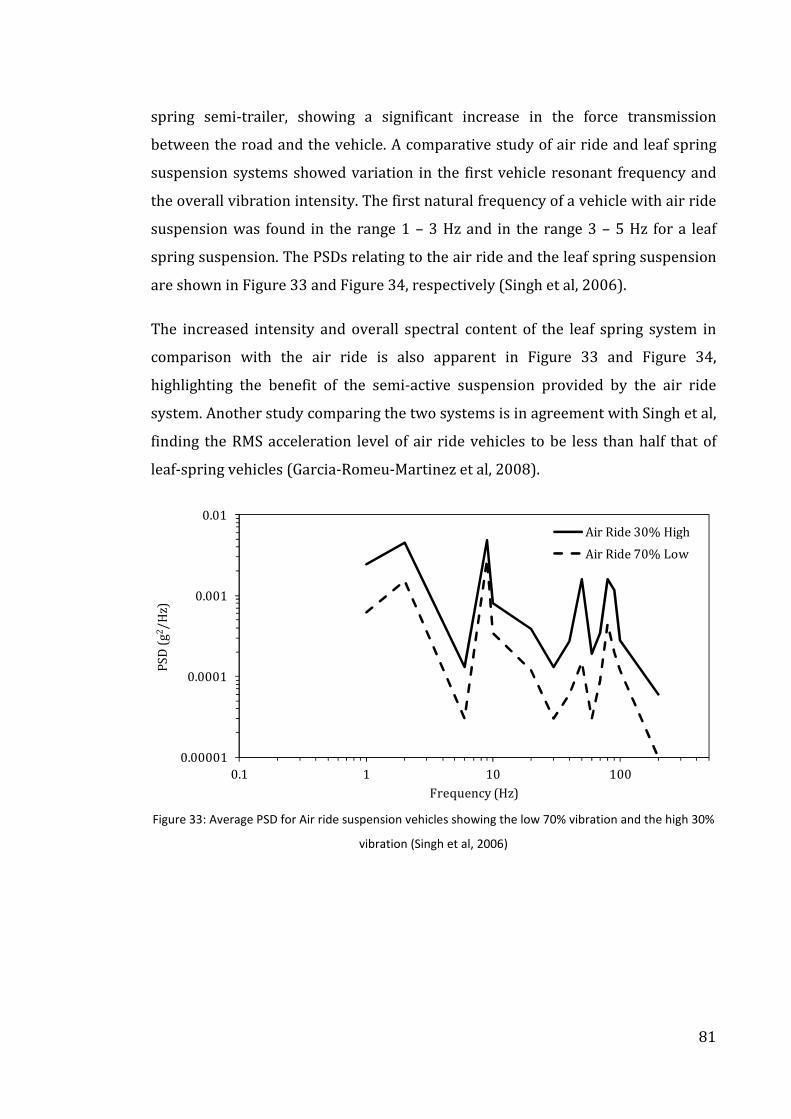
81
spring semi-trailer, showing a significant increase in the force transmission
between the road and the vehicle. A comparative study of air ride and leaf spring
suspension systems showed variation in the first vehicle resonant frequency and
the overall vibration intensity. The first natural frequency of a vehicle with air ride
suspension was found in the range 1 – 3 Hz and in the range 3 – 5 Hz for a leaf
spring suspension. The PSDs relating to the air ride and the leaf spring suspension
are shown in Figure 33 and Figure 34, respectively (Singh et al, 2006).
The increased intensity and overall spectral content of the leaf spring system in
comparison with the air ride is also apparent in Figure 33 and Figure 34,
highlighting the benefit of the semi-active suspension provided by the air ride
system. Another study comparing the two systems is in agreement with Singh et al,
finding the RMS acceleration level of air ride vehicles to be less than half that of
leaf-spring vehicles (Garcia-Romeu-Martinez et al, 2008).
0.00001
0.0001
0.001
0.01
0.1 1 10 100
PS
D (
g2/
Hz)
Frequency (Hz)
Air Ride 30% High
Air Ride 70% Low
Figure 33: Average PSD for Air ride suspension vehicles showing the low 70% vibration and the high 30%
vibration (Singh et al, 2006)

82
0.00001
0.0001
0.001
0.01
0.1
0.1 1 10 100
PS
D (
g2/
Hz)
Frequency (Hz)
Steel Spring 30% High
Steel Spring 70% Low
Figure 34: Average PSD for leaf spring suspension vehicles showing the low 70% vibration and the high
30% vibration (Singh et al, 2006)
3.9.3 Tyres
If imbalanced, tyre mass can cause undesirable vehicle vibration. These vibrations
are most apparent when travelling over 40 - 45 mph (Yokohoma, 2003). Tyre
misalignment can also cause a journey to be less smooth, leading to additional or
amplified vibrations.
Tyre stiffness can be affected by over or under inflation. The increases in stiffness
caused by over inflation results in a much harsher vibration response when
traversing over the road surface, particularly over large displacements as the tyres
are not able to isolate the effect of these as effectively. Over inflation of tyres
reduces traction which leads to reduced handling capabilities, and more severe
vibration response along all axes relative to the road. Cebon (1999) gives values of
tyre stiffness for different tyre constructions and pressures. The load, stiffness and
damping characteristics for different heavy vehicle tyre types, is given in Appendix
IV, Table 40.

83
The size of tyres can affect the ride quality. The smaller the diameter of the tyre,
the deeper the tyre will move into depressions and the quicker it will move over
obstructions in the road, leading to a rougher ride.
3.9.4 Payload
During a distribution journey, a vehicle’s payload can vary from being fully laden
to partially laden. This is particularly true in the case of home delivery or delivery
from a distribution centre to multiple stores. It is therefore important to consider
the effect that this change in payload has on the vehicle’s vibration response. Table
7 shows how increasing the payload decreases the average RMS value of the
vehicle’s vibration acceleration. This is expressed through the average RMS
acceleration level (Garcia-Romeu-Martinez et al, 2008). For the vehicle with an air
ride suspension, the added payload had the greatest effect between 0 - 40 km/hr
where the RMS acceleration decreased by 32%. For the vehicle with a spring-leaf
suspension, the added payload had the greatest effect between 40 - 70 km/hr
where a decrease of 26% was experienced.
Table 7: Results from a study carried out by (Garcia-Romeu-Martinez et al, 2008) on
vibration levels in Spain
VEHICLE PAYLOAD
RESULTING VIBRATION RMS ACCELERATION
(g) FOR EACH SPEED RANGE
0-40 km/hr 40-70 km/hr 70-110 km/hr
Air Ride (2 tonne) 0 Tonnes 0.068 0.087 0.093
Air Ride (2 tonne) 21 Tonnes 0.046 0.076 0.094
Spring-leaf (3 tonne) 0 Tonnes 0.212 0.238 0.254
Spring-leaf (3 tonne) 3 Tonnes 0.172 0.177 0.200
3.9.5 Vehicle Mass
Distribution vehicles range in size from a small family car to a large semi trailer.
The size of the intended distribution vehicle and its kerb weight will denote certain
other vehicle parameters, such as tyre pressure and suspension characteristics.
The effect of vehicle size and mass on its frequency response has been discussed in

84
section 3.5, where the variations between a standard car and small and medium
delivery vehicles, was evident. It has also been highlighted in the previous section
that a vehicle’s load level (payload) affects its vibration response.
3.9.6 Vehicle Speed
It has been observed in many studies that a vehicle’s speed greatly affects its
vibration response the higher the speed the greater the intensity of vibration
(Singh et al, 2008; Garcia-Romeu-Martinez et al, 2008; Rouillard 2008). This is
evident in Table 7, where the RMS acceleration was calculated for vehicles
travelling at different speeds (Garcia-Romeu-Martinez et al, 2008). The same
pattern can be seen in Figure 35, where the RMS acceleration measured in 5
second samples of a distribution journey and plotted against the vehicle’s speed
(Sek, 1996). There is a strong correlation between vehicle speed and RMS
acceleration, with the RMS acceleration increasing proportionally with speed up to
20 mph and between 40 to 60 mph. Between 20 to 40 mph, the RMS acceleration
remains approximately constant.
Figure 35: Variation of vibration severities with vehicle velocity, RMS acceleration (g) averaged over 5
second intervals (Sek, 1996)

85
A study by Lu et al (2010) also concluded that there was a positive correlation
between the RMS acceleration and vehicle speed, with the proportional increase in
the RMS acceleration being greater at lower speeds than higher speeds.
3.9.7 Drive Quality
Drive quality relates to the way in which the vehicle is driven. Poor drive quality is
the result of poor handling and driver errors such as hard braking, high speed
cornering and travelling over road hazards (e.g. speed bumps or potholes) at
speed. These can cause substantial shocks to the vehicle, amplify the effects of
adverse road conditions, and, can cause unnecessarily high rotational and linear
movement leading to excessive multi axis vibration of the vehicle. Human factors
and their effect on the vehicle response are extremely hard to determine, but
consideration of the variation in the quality of driving should be considered when
simulating a distribution journey. For instance, long duration distribution journeys
can cause driver fatigue. Studies have shown that driver fatigue results in slower
reaction times and low concentration. Driver fatigue can manifest itself through
poor driving or road traffic accidents (Hartley and Arnold, 1994; Philip et al, 1999).
3.10 Measurement
The previous sections have discussed the factors that affect and characterise the
vehicle’s response. In all of the experiments the response is measured using
accelerometers and data acquisition units. The measured response can be greatly
affected by: the type of sampling, whether continuous or timed or level triggered;
the rate at which data is sampled; and, the location in which the vibration is
measured.

86
3.10.1 Continuous vs. Sampled Data Acquisition
The most accurate way to capture a vehicle’s vibration response during a
distribution route is to acquire data continuously. By doing this, every event within
the distribution journey will be captured and can be analysed.
It has already been noted that vehicle vibration is highly unpredictable and if a
journey is repeated using a single distribution vehicle it will not be replicated
exactly, although the overall data averaged PSD is likely to be consistent. Since
distribution journeys are long in duration, the large quantity of data required to
accurately evaluate a single distribution route becomes apparent. For example, a
10 hour distribution journey with a sample frequency of 500 Hz, recording two
channels namely, the vertical vibration and the sample time, would require 360 Mb
of memory. If the GPS location and speed data are recorded every 5 seconds then
an additional 1.5 Mb is required. However, many data acquisition units used within
the distribution field are limited to a memory capacity which is much lower than
that required for this amount of data - for example, the Lansmont© Saver 9x30 has
a memory capacity of 128 Mb. Because of this limitation, data acquisition is
typically carried out using some form of data sampling, either, time triggered
sampling or trigger level sampling:
Time triggered sampling – where data are sampled at specified intervals for a
set period of time. There is no specified sample interval or size, both of which
have varied significantly across studies (Jarimopas et al, 2005), probably due to
data limitations and the length of the journey studied.
Trigger level sampling – data are monitored continuously and once a threshold
acceleration level is reached a sample of a set period is recorded. The choice of
acceleration threshold trigger also varies across studies depending on the type
and condition of the roads being monitored (Chonhenchob et al, 2012; Garcia-
Romeu-Martinez et al, 2008). The implication of using threshold trigger level
sampling is the possibility that the data will be biased towards higher
acceleration levels, and therefore the data appears more severe than might
actually be the case (Kipp, 2008a).

87
In some cases a combination of the two sampling techniques is used, but this can
also result in the data being biased towards the extreme vibration levels. It is
therefore wise to analyse the time and level triggered samples independently of
each other, using the level triggered samples to evaluate the extreme data and
treating the time sampled data as a means of evaluation (Rouillard and Lamb,
2008).
When using sampling, it is important that the sample rate, the sample size and/or
the trigger level are selected to suit the distribution environment being measured.
If the period between samples is too great, a poor representation of the
environment will be obtained. Parts (a) and (b) of Figure 36 illustrate the results of
time triggered sampling. Both have a sampling period of 60 seconds with different
sample sizes of 10 seconds and 2 seconds respectively. In both cases shock events
present in the full journey are missed out when sampling is used, this is
particularly true when using the 2 second sample size.
0 200 400 600 800 1000 1200 1400 1600 1800 2000-3
-2
-1
0
1
2
3
4
5
Time (seconds)
Acc
ele
rati
on
(g)
Continuous
Sample Period = 60s, Sample size = 10s
0 200 400 600 800 1000 1200 1400 1600 1800 2000-3
-2
-1
0
1
2
3
4
5
Time (seconds)
Acc
ele
rati
on
(g)
Continuous
Sample Period = 60s, Sample size = 2s
Figure 36: Example of time sampled data, 60s sample period (a) 10 second (b) 2 second sample size
(b)
(a)

88
This omission of critical vibration information is further evident in the RMS
acceleration distribution shown in Figure 37, where the shape of the RMS
acceleration distribution for the smaller sample size of 2 seconds does not show
good correlation with the RMS acceleration distribution of the continually sampled
data. This highlights the point that, by sampling at this rate, information in the
actual signal will be lost.
This shows that the higher sample size of 10 seconds gives a more accurate
representation of the full vibration signal, while a sample size of two seconds
produces a distribution that is focused around 0.1g with a much narrower spread
of data.
0 0.1 0.2 0.3 0.4 0.5 0.6 0.70
1
2
3
4
5
6
7
8
9
10
RMS (g)
Occ
ure
nce
(%
)
Sample Period = 60s, Sample Size = 2s
Sample Period = 60s, Sample Size = 10s
Continuous
Figure 37: RMS acceleration distribution of 1 second samples
The PSDs of the continually sampled signal and both alternative sample rates are
shown in Figure 38. Unlike the RMS acceleration distribution, neither PSD
produced using the two sample sizes follows the full vibration signal’s PSD exactly.
In this case the sample size of 2 seconds produces an underestimate of the signal,
while the sample size of 10 seconds, at points, overestimates the full signal’s PSD.
RMS acceleration (g)

89
100
101
102
10-6
10-5
10-4
10-3
10-2
10-1
Frequency (Hz)
Po
wer
Sp
ect
ral
Den
sity
(g2
/Hz)
Continuous
Sample Period = 60s, Sample Size = 2s
Sample Period = 60s, Sample Size = 10s
Figure 38: Average PSD’s for full signal and sampled signals
It is therefore apparent that continuous data sampling is the only sampling method
that will capture all events. Therefore, in order to create as accurate as possible a
representation of distribution vibration continuous sampling should be used. In
situations where this is not possible, Rouillard and Lamb (2008) state that in order
to produce an accurate statistical representation of a distribution journey, at least
1/8th of the journey data should be recorded at evenly spaced intervals, for
example, 2 seconds of data every 16 seconds.
3.10.2 Sample Rate and Frequency Range
The rate at which vibration data is sampled directly affects the frequency range
over which the signal can be analysed with the frequency being inversely
proportional to the sampling rate. In addition to this, when selecting a suitable
sampling rate, the issue of aliasing, where the signal being analysed becomes
distorted and false frequencies are detected, needs to be considered. Aliasing
occurs when frequency range exceeds the sample frequency. To eliminate aliasing,
the frequency range should be less than half the sampling frequency, this is often
referred to as the Nyquist or folding frequency (Smith, 1989).

90
The vibration range of interest for vehicle vibration is between 1 and 200 Hz,
therefore a sampling frequency of at least 400 Hz is required. This is consistent
with previous studies which have used a sampling frequency of 500Hz
(Chonhenchob et al, 2012), 651 Hz (Singh et al, 2007) and 1000 Hz (Garcia-Romeu-
Martinez et al, 2008).
3.10.3 Location of Accelerometers in the Vehicle
It is known that vertical vehicle vibration is most severe at the rear of the vehicle
on the kerb side (left hand side in the UK) (Zhou et al, 2007; Barchi et al, 2002;
Singh et al, 2007). This is consistent with overseas studies such as a study on
Indian roads which concluded that ‘….preliminary data collected showed that the
rear and kerb side location produced the highest levels of vertical vibration on most
highways that are generally two-lane, and have poor shoulders causing vehicles to go
over severe road imperfections’ (Singh et al, 2007).
The intensity of the vertical vibration can vary significantly depending on the
location in the vehicle. One study showed vibration at the rear of the vehicle was
14 times greater than at the front (Barchi et al, 2002). This difference is confirmed
by (Zhou et al, 2007) where the average RMS accelerations were found to be 1.91
m/s2 and 1.62 m/s2 at the rear and front of the vehicle, respectively. It is therefore
important that when recording vehicle vibration, the location of the accelerometer
is considered. If the position of the load is known, then the vibration at that point
should be measured or the worst case should be considered. Other studies have
measured the vibration at several points and presented it as an average (Bernad et
al, 2011) but whilst this allows all points in the vehicle to be considered, it may still
form an under test if loads are distributed unevenly across the vehicle floor.
In general, accelerometers are located in either two (front and rear) positions or,
three (front, middle and rear) positions. An exception to this was a study carried
out in Spain which measured the vibrations at the central span of the rear axle
(Garcia-Romeu-Martinez et al, 2008). Other setups have the accelerometers set at
100 mm from the right hand wall (Barchi et al, 2002; Berardinelli et al, 2004) and

91
200 mm from the right hand wall (Vursavus and Ozguven, 2004) - these tests were
carried out in Italy, Spain, France and Turkey where vehicles are driven on the
right hand-side of the road.
3.10.4 Measurement Equipment
In recent years, a large proportion of studies of vehicle vibration for the purpose of
distribution packaging testing have used a Lansmont© Saver data acquisition unit
(Singh et al, 2008; Singh et al, 2007; Singh et al, 2006; Chonhenchob et al, 2012).
This unit benefits from: being compact, with all equipment contained within the
unit; allowing fast transfer of data for analysis; and, being simple to use, with easy
selection of sampling and trigger levels. Since, as previously mentioned, the unit
has limited capacity memory (128 Mb), there must be compromise between
sampling rate, sample size and duration of recording, in order to ensure a full
distribution journey is recorded. Furthermore, as the unit contains a single tri-axial
accelerometer, vibration can only be measured at one location in the vehicle. This
is not an issue when a single axis of vibration at a set point is required, but when
the vehicle’s multi-axial motion is to be studied, then several units are required.
It follows that in order to create as accurate a representation of the distribution
journey as possible, the data acquisition equipment must fulfil the following
criteria:
• Move-ability of accelerometers – allows for data collection at any location
on the vehicle floor.
• Tri-axial and multiple single axis data recording – allows the vertical
vibration of the vehicle to be recorded in several positions at once and must
be flexible in allowing for tri axial data recording when required.
• High memory capacity –allows for continuous data collection on
potentially long duration distribution journeys, without the requirement for
data download during the journey.
• High speed data acquisition – allows for multiple channels of data to be
recorded together without affecting the acquisition rate.

92
• Non intrusive – being small and compact and not hinder loading and
unloading of the distribution vehicle.
3.11 Simulating Vibration in Laboratory Environment
Within the laboratory environment, vehicle vibration is simulated using either a
single axis, tri-axial or multi axes vibration table. The table controllers have the
capability of creating random vibration from a given PSD and more recently
developed controllers have the capability to carry out time replication of the
vehicle vibration. But, in many cases time history replication is usually an
additional software packaging and therefore not all new controllers have this.
Older controllers will not have the facility to carry out time replication, while older
test rigs may not have the capability.
One issue with current vibration controllers is that when reproducing time history
vibration they are limited to frequencies below 50 Hz (Kipp, 2001). In section 3.5,
it was stated that, for vehicle vibration, the frequency range of interest is from 1 Hz
to 200 Hz. Therefore when using time replication the frequencies above 50 Hz are
not represented in the simulation. Additionally, the vibration rigs are also limited
by the maximum stroke. On many vibration table, including those at Smithers Pira
and University of Bath, the maximum stroke is +- 75mm.
This means that when creating a new simulation method, these limitations must be
taken into account, so that the simulation method is created is usable on all
existing controllers. The simplest way to ensure the method is suitable is to:
1. Create a simulation method that incorporates random vibration simulated
from given PSDs.
2. Simulates vibration along only one axis at any one time.

93
3.12 Concluding Remarks
It is evident that the intensity and characteristics of vehicle vibration is influenced
by a number of journey and vehicle parameters. Furthermore, changes in these
parameters can have a significant effect on the vehicle’s response. When these
factors are considered, alongside the sensitivity of the vehicle’s dynamics, the
resulting vehicle vibration can be said to be highly varied and unpredictable.
Accounting for all of the various parameters is therefore important when
considering the simulation of a distribution cycle where numerous vehicle types
and geographic locations can be involved. One example is supermarket
distribution, where distribution vehicles can range from large heavy semi-trailers
to smaller delivery vans travelling between continents, countries or regions,
depending on the product. It is therefore apparent that in order to accurately
simulate vehicle vibration to test for the potential for product damage, the
experience of the packaged-product throughout each stage of the intended
distribution should be considered and accounted for. This includes road, vehicle
and driver characteristics.
This variation in vehicle vibration between vehicles types and distribution
journeys emphasizes the need for accurate data acquisition that reflects the
intended distribution. In order to recreate a journey as accurately and as
confidently as possible, continuous data acquisition should be used. If sampling is
used then careful consideration must be given to the sample interval and size.
Furthermore, it is clear that inadequate data acquisition or misplaced
measurement equipment can severely manipulate the measured vibration
amplitude and characteristics. It is therefore essential that when measuring vehicle
vibration the position of the packaged product and its loading are considered
ensuring as representative a measurement as possible.
Vibration in the vertical axis is the most dominant and therefore considered to
have the most damage potential. It is therefore often the case that only the vertical
vibration is considered. In reality any point on the vehicle floor is subjected to six

94
degrees of freedom in its movement. Previous work has shown vibration along the
other two linear axes – lateral and longitudinal; and, the rotational axes - pitch, roll
and yaw; to be less significant than the vertical. However, when considering the
loading arrangement of packaged products their effects can be more significant
and therefore the effect of the MDOF vibration on product damage should be
examined.
With an understanding of vehicle vibration, the established method set out in the
existing testing standards for simulating vehicle vibration for the purpose of
packaging testing, along with other suggested approaches, can now be evaluated.

95
4 A REVIEW OF SIMULATION METHODS
Kipp (2008b) posed the question: ‘How can we create meaningful random vibration
profiles for laboratory testing, while at the same time accounting for, and simulating
the effects of: varying amplitudes, different characteristics, and infrequently-
occurring large-amplitude motions?’.
This question has become more pertinent for two reasons in particular:
• increased pressure on packaging engineers to create optimal packaging
solutions that are sustainable - economically, environmentally and socially
• the evolving capabilities of computers and laboratory equipment which
make the use of more complex simulation methods possible, which has
enabled more in depth research into the behaviour and nature of vehicle
vibration.
More recent research has led to dissatisfaction with the established method which
is currently used to simulate vehicle vibration for packaging testing. This in turn
has resulted in the creation of a number of alternative simulation methods that are
seen to improve on the shortcomings of the established method.
An in depth review of both the established method, which underpins the ISTA and
ASTM standards, and, several alternative methods, proposed in the literature, has
been undertaken in order to establish their relative capabilities together with their
limitations.
4.1 A Critique of the Established Method
Post 1980’s, accelerated random vibration testing, utilising Gaussian signals
produced from PSDs (Accelerated Gaussian Equivalent Method), has been the
norm in distribution packaging testing and underpins both the ISTA and ASTM

96
vibration testing standards. The established method of building a simulation using
this method can be summarised as follows:
Step 1: Data from multiple distribution journeys is collected.
Step 2: The FFT is then used to convert the signals from the time to the frequency
domain. The DFT which underpins the FFT is given in Equation 12 and is
stated here for completeness.
rtkfiN
rrk etxfX
π2
1
)()(−
=∑=
The length of the DFT (the number of data points over which it is
calculated) denotes its frequency resolution so that the larger the DFT (N)
the higher the resolution, where the frequency resolution Δf = 1/(Ndt).
Step 3: The PSD is then calculated using Equation 15, which is the calculation of
the product of the DFT spectrum, X(f), with its conjugate (X*(f)) divided
the length of X(f), (N), multiplied by the sample interval (Δt).
)(*)()( fXfXN
tfS •
∆=
Step 4: The PSD spectra from multiple signals can then be averaged together, the
equation for which is given in (Garcia-Romeu-Martinez et al, 2008).
∑=
⋅=n
ii fS
nPSD
1
)(1
(17)
where n is the number of spectra being averaged so that i = 1,2,3,...,n.
Step 5: In order to reduce long test durations, tests are time compressed (test
accelerated). Test acceleration is carried out based on the representation
of accumulated damage, where damage can be measured as the stress
levels and the number of cycles leading to some critical level at which the
product fails. The stress level compared with the number of cycles to

97
failure (S - N) curve is used in most fatigue theory concepts. For most
specimens of a single material and configuration a large part of the S - N
curve can be approximated by the Basquin expression (Basquin, 1910):
K
rSfNm = (18)
where Nf is the fatigue life at stress level Sr, K is the slope factor of the
curve and m is the material constant, which is dependent on the material
being tested.
Using the Basquin expression in Equation 18, a relationship between test
duration and intensity (RMS acceleration) is constructed. This equation
can then be used to accelerate the test (Shires, 2011). The increase in test
intensity is inversely proportional to the reduction in test duration
following the power law. This is specified in the military standards (MOD,
1999).
K
Actual
dAccelerate
dAccelerate
Actual
RMS
RMS
T
T
= (19)
A widely adopted approach, and what it is assumed is used in the existing
test standards, is to set K at 2 and the time compression by five (Kipp,
2000).
Unfortunately, there is currently no accurate way to measure the amount
of accumulated damage or the rate at which it grows. Additionally,
different materials have different fatigue rates, with the fatigue rates of
samples of the same material varying due to differences in construction
and quality. Because packaging is typically constructed of several
materials each with a different fatigue life, the process of calculating
fatigue rate is further complicated. These limitations mean that by using
fatigue theory to accelerate the test it is necessary to assume that for each
product, each packaging system is identically constructed and that the
packaging system acts as a single material.

98
Step 6: A vibration signal can now be created using the accelerated average PSD.
This is done by firstly rearranging Equation 15 to find the magnitude of
the Fourier spectrum using the accelerated PSD.
NdtfSfX )()( =
Because when calculating the PSD the Fourier spectrum’s phase
information is lost, a random phase array must be applied to form the real
and imaginary parts of the spectrum. Following this Equation 11 for the
inverse DFT can be applied and a signal, of length N can be calculated. The
processes in step 6 are then repeated until a signal of the required length
(duration) is produced.
Rouillard (2007) states that the PSD ‘...does not contain information on
time-variant parameters such as possible variations in amplitude or
frequency or the time at which these variations occur. Furthermore, the
temporal averaging process inherent to the PSD cannot separate the effects
of transients within the signal'. Therefore when using this technique to
construct a time domain signal, the signal will always be stationary signal
with a normal (Gaussian) distribution.
Figure 39 gives an example of how the established method is used and illustrates
how the vehicle vibration (original signal) (a) varies from the simulated signal
(equivalent Gaussian signal) (c). The reduced spread of acceleration levels is
evident in the equivalent Gaussian signal with the defined shock events that were
present in the original signal now not present. Additionally, the PSD presented in
the testing standards (Figure 157 and Figure 158) is much simpler than the PSD
shown in Figure 39. This is due to the use of spectral smoothing reducing the
number of breakpoints used to define the spectral shape. This simplifies the shape
of the PSD, making it easier to compile spectra and reducing the computational
time required to run a simulation.

99
Figure 39: Example use of the accelerated Gaussian equivalent method
As previously discussed in section 3.7, accounting for the variations in distribution
journeys is increasingly important. As a consequence of this, ISTA introduced test
4AB. When enough information about the intended distribution is available, this
test allows the user to construct their own vibration PSD from historical data, so
that a more relevant vibration test to be produced (ISTA, 2010). It is important to
note that in order to create an accurate test with confidence, a large amount of
0 50 100 150 200-2
-1.5
-1
-0.5
0
0.5
1
1.5
2Original Vibration Signals
Time (seconds)
Acc
ele
rati
on
(g)
100
101
102
10-8
10-6
10-4
10-2
100
Frequency (Hz)
Po
wer
(g2
/Hz)
Average PSD
Accelerated PSD
0 10 20 30 40 50 60-2
-1.5
-1
-0.5
0
0.5
1
1.5
2
Time (seconds)
Acc
eler
atio
n (
g)
(c) Accelerated Gaussian Equivalent
(b) Average PSD and accelerated averaged PSD
(a) Original signal

100
journey vibration data is required. Therefore, data collection on the intended
distribution journey would need to be repeated several times to gain this
confidence. The more times the journey was repeated, the higher the statistical
significance of the resulting simulation.
4.1.1 Benefits of the Established Method
In section 3.7 the idea that no two distribution journeys will produce the same
vibration is presented. A key benefit of the established method is that it lends itself
easily to averaging. By creating a PSD from the vibration measured over several
journeys, an averaged PSD with statistical significance and hence confidence can
be produced (Kipp, 2001).
It would often be uneconomic and impractical to simulate the full duration of a
distribution journey when testing packaging. By using test acceleration, the
established method allows for a significant reduction of the test duration and the
associated costs.
Furthermore, the simple nature of the method makes it straightforward to
implement with the majority of laboratory controllers having the capabilities to
execute the method.
The established method has been in use for many years and although it is limited
in its ability to simulate shock induced damage or the complex variations in
modern distribution, these points are generally well known and can be
compensated for through conservative or over compensatory packaging design.
4.1.2 Limitations of the Established Method
Although there are benefits to the established method, it is subject to several
limitations relating to the method and its application in the testing standards.
A key limitation is the nature of the simulation the method produces. The non-
stationary and non-Gaussian nature of vehicle vibration has been discussed in

101
section 3.2. By simulating this vibration as stationary with a Gaussian distribution
the high level acceleration events, which give vehicle vibration its non-Gaussian
distribution, are absent. This means that the overall spread of acceleration levels
changes, with actual vehicle vibration tending to have a distribution with longer
tails and a sharper peak, while the simulated signal follows a bell shaped Normal
distribution.
Additionally, a constant RMS acceleration level is used throughout the test. For
actual vibration the RMS acceleration level will constantly fluctuate. Ultimately,
this means that key characteristics of vehicle vibration are not simulated in the
established method and hence the simulation produced is not an accurate
representation of vehicle vibration. Simulating vibration in this way may
manipulate fatigue damage or result in threshold level damage caused by high
level acceleration events being neglected. While this limitation is known and can
therefore be compensated for, the method cannot be used to optimise a packaging
solution.
Furthermore, the fatigue theory used to accelerate the tests is not designed for the
complex material construction of packaging and therefore may not be directly
applicable to its application. This could lead to inaccurate simulation of product
damage.
Whilst there are limitations regarding the method, the way in which it is applied in
the testing standards is also limited. The standards use universal PSDs to simulate
all semi-trailers with leaf spring suspension, or, all semi-trailers with air ride
suspension, therefore not accounting for the variations in vehicle dynamics
apparent between vehicles and payloads. Furthermore, using a single test to
represent all distribution journeys may lead to cases of both over and under
testing.

102
4.2 Improved Methods of Simulation
Many simulation methods have been proposed and developed to improve on the
limitations of the established method. These can be grouped under six headings:
time replication; two way split spectra; three way split spectra; shock on random;
kurtosis control; and, RMS modulation.
4.2.1 Time Replication
Used in the automotive transport sector, to test for noise, durability, vibration and
harshness, time replication testing requires the laboratory reproduction of a
continuous time domain vehicle vibration for a given distribution journey. This
allows for the complete recreation of the journey, which is therefore not
‘statistically compromised’ (Bernad et al, 2011).
Whilst this may be beneficial for automotive testing, past studies into distribution
vibration have shown that vibration intensities and characteristics vary between
journeys due to changes in vehicle parameters and road conditions (Garcia-
Romeu-Martinez et al, 2008). Therefore, using the time replication of a single
journey would not sufficiently represent all journeys. A comparison of two
journeys carried out on the same distribution route in the same vehicle is given in
Figure 40 and Figure 41. Whilst the overall RMS acceleration for each journey was
relatively similar at 0.197 and 0.207, respectively, the kurtosis of the signals varies
dramatically, from 18 to 50 due to the presence of extremely high level shock
events recorded on the second journey.
0 200 400 600 800 1000 1200 1400 1600 1800 2000-6-4-202468
10
Time(seconds)
Acc
eler
atio
n(g
)
Figure 40: Vibration signal recorded on journey 1

103
0 200 400 600 800 1000 1200 1400 1600 1800 2000 2200 2400-6-4-202468
10
Time(seconds)
Acc
ele
rati
on
(g)
Figure 41: Vibration signal recorded on journey 2
Whilst the first journey may underestimate the severity of the journey, the second
journey may be an over estimate. As a consequence there is a lack of confidence in
the use of either signal. In order for there to be some level of confidence, multiple
journeys on the distribution route must be recorded and evaluated, to approximate
an ‘average’ journey. The data acquisition requirement for this method is time
consuming and expensive and is therefore impractical for most products.
4.2.2 Two Way Split Spectra
Splitting the simulation PSD to form two spectra created from the lower and higher
amplitude portions of vibration was first proposed by Young et al (1998). The
method has further been used in a number of subsequent studies (Singh et al,
2006a; Chonhenchob et al, 2012). These studies created the two spectra based on
the 70% low data and 30% high level data. A different study took a ‘more stringent
approach’ and split the spectra 80-20% (Wallin, 2007).
This method partially alleviates the issues relating to the established method by
enabling testing to be carried out at a high acceleration level for a period of the
test. This goes some way towards recreating the high level data that is modulated
during. Additionally, it produces a signal that when considered as a whole is non-
stationary and non-Gaussian. In reality the simulated signal is Gaussian and
stationary for substantial periods of the total test. Importantly, the method is again
based on averaged data and therefore a moderated signal is still produced, with
the variation between high acceleration shock events and low level vibration not
simulated accurately.

104
4.2.3 Three Way Split Spectra
An advance on the two way split spectra, a three way split, has been proposed.
Here the signal is split into three parts leading to spectra of the lower 70%,
intermediate 25% and top 5% of data. Arguably, this approach allows for better
simulation of the overall vibration acceleration distribution and, in particular, the
higher level events (Kipp, 2008b). Although in essence it still produces Gaussian,
stationary signals for the greater part of the simulation.
Additionally, simulating all high level events consecutively could lead to unrealistic
predictions of product fatigue or threshold level damage.
4.2.4 Shock on Random
Shock on random combines the established method with shock superposition. A
PSD of the signal is used to create a random, stationary signal with a Gaussian
distribution, representing the average vibration. Shock events recorded from the
distribution journey are then integrated at random points within the signal,
thereby allowing a signal with a non-Gaussian distribution to be produced and the
high level shock events to be simulated (Kipp, 2001).
The benefit of this method is that it allows the input of realistic high level shock
events in a manner similar to how they occur during actual vehicle vibration,
therefore allowing for the impact that shock events have on product damage or on
the activation of product damage.
Although the method allows for the non-Gaussian nature of the signal to be
presented, the question of how many shocks and when they are imposed has to be
asked. In order to confidently recreate the shock events on a particular
distribution journey, it would be necessary to record vibration on several journeys
to ensure an accurate view of the distribution journey is obtained. This exercise
would be time consuming, costly and therefore inefficient.

105
4.2.5 Kurtosis Control
The established method produces a vibration signal with a kurtosis of 3. In section
3.4 the kurtosis of vehicle vibration was shown to be much higher. By applying
Kurtosis control, the amplitude of higher acceleration events can be increased,
resulting in a higher signal kurtosis. The generated signal would therefore have a
similar acceleration distribution to vehicle vibration, although the sequence is
statistically stationary. Van Baren (2005) describes a method of kurtosis control
entitled ‘Kurtosion’ where a simulated signal is formed based on a given PSD, RMS
acceleration and kurtosis parameter. The kurtosis parameter is used to increase
the spread of the simulated signals acceleration PDF.
4.2.6 Modulated RMS Distribution
The RMS acceleration distribution of a vehicle vibration can be seen in Figure
42(c). Here the highly non-stationary nature of the vibration is evident. RMS
modulation, randomly applies the statistical RMS acceleration distribution of the
original vibration signal to create a non-Gaussian and non-stationary simulation
signal constructed from short-time, stationary segments with a Gaussian
distribution (Rouillard, 2007b).
Rouillard and Sek (2010) presented the development of the Statistical Vibration
Synthesizer (SVS) module that can be incorporated into existing controllers and
simulation tables, to create a modulated RMS simulation. The module randomly
amplifies the table’s drive signal to match the RMS acceleration distribution of the
signal being simulated. A screen shot of the controller in use is provided in Figure
42. The computer system shows the real time: drive signal (a), PSD (b), RMS
acceleration distribution of the simulated signal (c), RMS acceleration level (c) and
the signal’s PDF (d).

106
Figure 42: Screenshot of the SVS module computer system, showing real time (a) drive signal (b) PSD (c)
RMS acceleration distribution (d) PDF
Results in Rouillard and Sek (2010) showed that the simulation produced through
the SVS module correlated well with the original signal.
The main limitation of this method is that of controller capability which limits the
speed at which the RMS acceleration level can be changed and hence the duration
for which it is held. Furthermore, an accurate measure of the RMS acceleration
distribution and the PSD that describes the distribution journey is required.
4.3 Concluding Remarks
In order to optimise a packaging solution, a high level of confidence in the method
of simulation is required. The established method of vibration testing for
distribution packaging creates a simulation that is based on the average frequency
and amplitude content of vehicle vibration. It then reduces test duration using an
acceleration method based on fatigue theory. This has been shown to result in a
simulation which, in contrast to vehicle vibration, is stationary with a Gaussian
a b
c
d

107
distribution, and therefore does not create a realistic simulation. Thus the
limitations of the established method can result in conservative packaging design.
Simulation approaches suggested in recent and past literature highlight the
inefficiencies of the established method and suggest methods of improvement.
Many of these approaches use the same theory as the established method, but in
addition utilise an improved statistical representation. This includes: the two way
split spectra; three way split spectra; RMS modulation; and, shock on random. All
of these approaches combine the established method with some form of additional
statistical consideration.
Unfortunately, although it is suggested that these improved approaches are
superior to the established method, there is little evidence of their benefits
through application in physical testing and therefore they lack the user confidence
that the established method possesses. In order to gain confidence in these
improved simulation methods and additionally evaluate their use, correlation
studies measuring actual product damage need to be carried out. The results of
such studies are presented in Chapter 5.

108
5 AN EXPERIMENTAL COMPARISON OF
THE DAMAGE CORRELATION OF
SIMULATION METHODS
The objective is to understand how the various simulation approaches previously
reviewed correlate with each other and with a benchmark time replicated journey.
For the purpose of the study a single damage mechanism of scuffing is considered.
Scuffing is used because it is generally accepted to be a cumulative form of damage.
Previous work by Shires and White (2011) have generated and validated a design
for a scuffing measurement rig. By measuring one overarching damage mechanism,
the process of calculating damage is simplified.
5.1 Experimental Method
A continuous time record for a reference journey was used as the benchmark of
this study, the damage produced by the time replication simulation was then
compared with the damage produced by simulations created using the following
simulation approaches:
• modulated RMS Distribution (Rouillard and Sek, 2010)
• two Way Split Spectra (Wallin, 2007)
• three Way Split Spectra (Kipp, 2008b)
• single Level PSD (established method non-time compressed)
• accelerated Single Level PSD (established method) – where K = 2 and time
compression of 5 (Kipp, 2000)
• accelerated Single Level PSD (established method) – where K = 4.7 and
time compression of 5

109
The reference journey was recorded on a Ford Luton Box van travelling at an
average speed of 64 km/hr (40 mph) along a 32 km mix of roads in the city of Bath,
UK (summary journey record shown in Figure 43). The data were sampled
continuously at a rate of 2000 Hz. The resulting vibration signal was then filtered
between 1 - 200 Hz.
0 200 400 600 800 1000 1200 1400 1600 1800-2
-1.5
-1
-0.5
0
0.5
1
1.5
2
2.5
3
Time (seconds)
Acc
eler
atio
n (
g)
Figure 43: Time history for reference journey
The distribution of the RMS acceleration for one second samples was calculated.
One second samples were taken from the signal with an overlap of N-1 data points,
where N is the number of data points in a one second sample. An example of the
sampling process is shown in Figure 44, where the first sample of length N
includes data points 1 to N, the frame is then moved to provide an overlap of (N-1)
so the second sample includes data points 2 to N+1. Overlapping the signal
samples allows any variations in the RMS acceleration to be captured, so that a
complete representation of the RMS acceleration distribution can be produced.

110
0 1 2 3 4 5 6 7 8 9 10 11 12 13 14 15 16 17 18 19 20-1
-0.50
0.51
Time (second)Acc
ele
rato
n (
g)
1— N
2— N+2
3— N+3
Data sample 1
Data sample 2
Data sample 3
Figure 44: Example of data sampling with window length (N) with an overlap of (N - 1)
The RMS acceleration distribution for the vibration signal in Figure 43 is displayed
in Figure 45, illustrating the percentage occurrence of RMS acceleration levels for
one second samples. The percentage occurrence of RMS acceleration intensities is
given in Table 8. The variation in the RMS acceleration distribution highlights the
non-stationarity of the time history signal.
0 0.1 0.2 0.3 0.4 0.5 0.6 0.70
5
10
15
20
25
RMS(g)
Occ
ure
nce
(%
)
Figure 45: RMS acceleration distribution for reference journey
The signal’s overall PSD, is then calculated as the average of each signal segment’s
PSD.
Sample number
RMS acceleration (g)

111
∑=
⋅=n
i
iPSDn
PSD
1
1 (20)
Where:
n = the number of signal segments, which is equal to the length of the signal
minus the overlap used (N – 1)
i = 1, 2, 3, ..., n
To simplify the PSD, it is described using a reduced number of points that
represent its overall shape. The average PSD for the signal is illustrated in Figure
46. The PSD breakpoints are given in Table 9.
100
101
102
10-6
10-5
10-4
10-3
10-2
Frequency (Hz)
PSD
(g
2/H
z)
Figure 46: Average PSD for reference journey

112
Table 8: RMS acceleration distribution with
levels in order of test
Table 9: PSD break points
RMS
ACCELERATION
(g)
RMS
ACCELERATION
OCCURENCE (%)
FREQUENCY
(Hz)
PSD
(g2/Hz) (x10
-5)
0.294 2.9 1 39.8
0.140 24.1 2 397
0.063 11.8 3 1020
0.178 17.7 5 75.0
0.449 0.6 8 23.4
0.626 0.6 10 56.3
0.410 0.6 15 89.2
0.217 9.4 20 12.0
0.1017 19.4 22 6.06
0.0247 11.8 30 2.02
35 10.0
50 8.80
70 2.50
80 0.502
90 0.237
100 0.496
150 0.108
200 0.194
Vibration tests were conducted using a Team servo hydraulic vibration testing
machine (Team Corporation, Burlington, USA) controlled by an M&P VibPilot
Controller (M&P International, Hannover, Germany). Tests were created using the
simulation techniques and the test conditions summarised in Table 10.
Table 10: Simulation methods with RMS acceleration levels and test durations
NO TEST METHOD
RMS ACCELERATION
(g)
DURATION
(Minutes)
1 Time Replication 0.17 30
2 Modulated RMS See Table 8 30
3 Two Way Split Spectra 80-20% 0.16 & 0.25 30
4 Three Way Split Spectra 75-20-5% 0.16, 0.22 and 0.39 30
5 Single Level PSD 0.17 30
6 Accelerated Single Level PSD (x5) K = 2 0.37 6
7 Accelerated Single Level PSD (x5) K = 4.7 0.23 6

113
5.2 Design of the Scuff Rig
The damage mechanism of scuffing was measured using a purpose built scuffing
device. The design and validation of the scuffing device has been described
previously (Shires and White, 2011). Details of the design and its validation are
also given here for completeness.
The principles sought in the design of a vibration response device are:
1. it should have a measurable response to vibration input, within the range of
vehicle vibration (1 – 200 Hz);
2. it should simulate a response to vibration seen in the distribution of
packaged goods such as scuffing or bruising;
3. its response to vibration should vary with both input intensity and input
duration in a repeatable and measurable way.
The device exploits the transfer of ink from a printed to a non printed surface as a
result of relative surface motion in response to vibration, which closely relates to
print scuffing in packaged goods distribution.
Parts (a) to (c) of Figure 47 illustrate the evolution of the rig design. A printed
sheet of board is mounted on mass W1 and an unprinted sheet of board on mass
W2. The masses are held together under pressure such that the printed and
unprinted boards are in contact. The masses are mounted on different stiffness
springs such that they move relative to each other in response to vibration. Figure
47(b) represents a simplification of the system in Figure 47(a) in that one mass is
rigidly coupled to the vibration input. However, both systems present two
concerns:
• They may be under-damped compared with packaged goods.
• They will be prone to complex off-axis vibration responses.

114
Off-axis vibration might be controlled by using linear guides, but these would
increase the design complexity, may inhibit system response to low vibration
levels and may present a design challenge in avoiding unwanted structural
resonances.
Replacing the springs with foam cushions increases system damping (and arguably
similar to cushioned packaged goods), but compressive creep in the contact
pressure cushion could result in change in contact pressure and poor repeatability.
The design in Figure 47(c) rotates Figure 47(b) by 45 degrees and replaces the
springs with a cushion material such that the contact pressure results from the
normal component of the test mass (the cushion above the weight applies only
slight pressure to prevent bouncing or chattering). The component of the mass
parallel to the inclined plane was matched to the cushion such that the mass and
cushion corresponded to an optimised cushion design (Goodwin and Young, 2011).
The system will be less prone to error from small levels of compressive creep in
the support cushion as the pressure is set by the mass.
A schematic of the device is shown in Figure 48 and images of the constructed
device are shown in parts (a) to (d) of Figure 49.
W1
1 W2
1 W2
1
W2
1
Cushion
Material
Test Samples
a
1a
b c (b)
Test sample
Cushion material
(a) (c)
Figure 47: (a) – (c) Possible designs of test rig

115
Cushion material is positioned in the box, as in Figure 48 so the mass responds to
vibration input in a manner similar to a packaged item with cushion shock
protection. A foam block polyethylene (PE), with a closed cell density of 75 kg/m3
was used to provide cushioning. The foam was selected based on the mass used to
optimise cushion performance (and the scuffing potential).
Cushion Material
Ivorex high white uncoated board
Mass
Smooth ‘printed’ clay-coated board with sun ‘blue 10’ flexo ink
Cushion Material
Closed metal lidded container
Metal frame (set at 450 to the horizontal)
Figure 48: Scuffing test rig schematic

116
Figure 49: (a) Metal box with Ivorex card attached, with foam cushion (b) Cubic mass loaded in metal
box, (c) Inclined metal box fixed to vibration table, (d) 25kg mass with smooth ‘printed’ clay-coated
board with ‘sun 10’ flexo ink
5.3 Quantifying the Level of Scuffing
Following a test, the degree of scuffing is measured by summing the total blue
content of all the pixels on the Ivorex card (Figure 50).
(c)
(b) (a)
45o
Ivorex high white uncoated board
Cushion
material
Mass
Closed metal
lidded container
Metal frame at 45o
Smooth ‘printed’ clay-
coated board with
‘sun 10’ flexo ink Mass
(d)

117
Figure 50: Ivorex card with scuffing after simulation
A computer program was used to count the blue pixels. This process was:
1. Scan the Ivorex card as a glossy photo with a resolution of 600 dpi.
2. Load scans on PC as a PDF and enlarge so that the entire PC screen is filled
with the scuff damaged area.
3. Crop the scanned image so that it includes only the 15 cm x 15 cm area that
was in contact with the mass.
4. Save cropped area as a Jpeg file.
5. Determine the percentage scuffing executed using Matlab code. The process
is:
a. Load the saved Jpeg file, automatically displaying the image as a
count for red, green and blue (rgb) for each pixel.
b. Sum the b count of all pixels to find the total blue value (B).
c. Calculate the percentage scuffing, which is the reduction in the total
blue pixel count (B) in proportion to the total blue pixel count for a
blank white Ivorex card of the same size (C).
Ivorex high
white uncoated
board
Ink transfer
from scuffing
damage

118
Scuffing=C
B1001 ×
− (21)
The level of blue ink transferred indicates the severity of the test i.e. the higher the
level of blue transferred the more severe the test (Shires and White, 2011).
5.4 Validation and Repeatability of Scuffing Rig
The rig was subject to a range of investigative tests to assess its response to
vibration intensity and vibration time and repeatability.
The scuff rig was checked for repeatability by repeating a test at one intensity and
duration ten times. The image analysis method was checked separately for
repeatability by scanning and analysing the same sample ten times. The test gave
repeatability better than 95% and the image analysis better than 99%.
The pattern ink transferred to the Ivorex board reflected localised pressure
variability from the machining of the adjacent parts. This pattern could be
eliminated by mounting the samples on resilient backing material, but the
progression of scuffing was substantially slower. For practical purposes the
scuffing pattern was therefore accepted, but this represented a possible barrier to
inter-laboratory repeatability.
5.5 Scuff Correlation between Simulation Methods
The high level of repeatability through use of the rig meant that each simulation
method was tested once only. Time replication (band 1, Figure 51) resulted in
0.59% additional blue as a result of scuffing. Both the modulated RMS (band 2,
Figure 51) and, the accelerated single level PSD with a time compression of 5 and K
= 2 (band 6, Figure 51), produced a similar level of damage to the time replication
with 0.56% and 0.64% respectively. The three way split spectra produced the
largest over test and the single level PSD produced the greatest under test at

119
0.81% and 0.1%, respectively. The variation in each test (simulation methods 2 – 7,
Table 10) with respect to time replication (simulation method 1, Table 10) is
shown in Figure 52.
Figure 51: Percentage scuffing for the simulation techniques
Figure 52: Percentage variation in scuffing for each simulation method compared to time replication

120
The results are consistent with the theoretical modelling of Shires (2011) who
predicted that single level (non-time compressed) tests would represent an under
test and that time compressed tests based on an assumed value of K = 2 would
have a much lower error than expected from a comparison of average journey and
test levels.
5.6 Concluding Remarks
The level of scuffing damage produced, varied between simulation techniques. The
simulation approaches that gave best correlation with the benchmark time
replication were the Modulated RMS and the established method using an
accelerated test with K = 2.
The greatest error in a test resulted from the single level, non-time compressed
approach and the single level time compressed test using a value for K = 4.7. These
produced a significant under test, resulting in 82% and 70% less scuffing than time
replication, respectively. Also of importance is the variation in scuffing produced
between the two accelerated tests where K = 2 and 4.7, respectively. This indicates
that the selection of K can induce significant errors in the packaging testing and
that therefore careful consideration of the value selected should be given.
The results suggest that by using a more complete decomposition of the signal e.g.
the RMS modulation method, rather than the two way or three way split spectra,
error in the simulation can be reduced, and therefore, a more accurate
representation of the vehicle vibration can be created. Both the two way and three
way split spectra tests resulted in significant error, this is because the two way
split test excluded the higher level events, and, the three way split over tested the
higher 5% of the signal.
Whilst many approaches have considered the variation in signal RMS acceleration,
they have not considered the variation in signal frequency content at difference
RMS acceleration levels. The frequency content of a signal can have a significant
effect on the product response due to resonance (section 3.5). Therefore, while the

121
RMS modulation approach produced a small amount of error (5% less scuffing
damage than the time replication) it may still be improved upon by considering the
variation in frequency content associated with the RMS acceleration levels.
Furthermore, each of these approaches considers only vibration with a Single
Degree of Freedom (SDOF), along the vertical axis. In reality vehicle vibration has
multiple degrees of freedom (MDOF). It is therefore necessary to consider the
effect of vibration along the additional linear axes and vibration around the
rotational axes, on product damage. A case study evaluating the need for MDOF
testing has been carried out.

122
6 EVALUATING THE NEED FOR MDOF
TESTING
The random and varying nature of a road surface means that vehicles and their
corresponding payloads experience MDOF vibration, including along three linear
axes: longitudinal (X); lateral (Y); and, vertical (Z); and, around three rotational
axes: pitch; roll; and, yaw. These are illustrated in Section 3.6, Figure 27.
Current packaging test standards – ISTA, ASTM, EU, BS, Chinese and Japanese etc;
simulate vehicle vibration using a SDOF in the vertical direction. The reasoning
behind this is that the acceleration along the vertical axis is generally much greater
and therefore considered to be more significant than in either the lateral,
longitudinal or rotational axes.
This assumption is supported by the empirical comparisons of vehicle linear tri-
axial vibration, given in section 3.6, which showed vibration acceleration to be
predominant along the vertical axis, with longitudinal and lateral vibration being
markedly less significant. This is most evident in the frequency range 1 – 20 Hz
(Singh et al, 2006). A recent study concluded that in the frequency range 1 – 10 Hz,
the neglected acceleration when using a vertical excitation only, was not
significant. However, above this range the additional acceleration from the
application of multiple axis vibration is significant (Bernard et al, 2011).
Figure 53 gives an example recording of the tri-axial vibration measured in a
delivery vehicle. It is evident that the magnitude of the vibration and shock along
the vertical axis is much greater than that along either the lateral or longitudinal
axes.

123
0 10 20 30 40 50 60 70 80 90 100 110-1
-0.5
0
0.5
1
1.5
Time (seconds)
Acc
eler
atio
n (
g)
0 10 20 30 40 50 60 70 80 90 100 110-1
-0.5
0
0.5
1
1.5
Time (seconds)
Acc
eler
atio
n (
g)
0 10 20 30 40 50 60 70 80 90 100 110-1
-0.5
0
0.5
1
1.5
Time (seconds)
Acc
eler
atio
n (
g)
Vertical
Lateral
Longitudinal
Figure 53: Vertical, lateral and longitudinal vibration signal
The acceleration power of the vibration on each axis is displayed in Figure 54
using the PSD of each signal. When comparing the PSDs the power within the
vibration (where power is measured as the vibration acceleration squared (g2))
along the vertical axis can be seen to be much greater than that along the lateral
and longitudinal axes, specifically in the range 1 - 20 Hz. Above this range the
variation in the power is less significant. Also evident in Figure 54 is the location of
the key frequencies for each of the axes. The vehicle has three predominant
resonant frequencies, which were discussed in section 3.5. The first of these can be
seen in Figure 54 at around 2 Hz, the second frequency is then visible in the

124
vibration of all three axes around 10 - 20 Hz, the discretisation of the spectra
makes the exact location of the peaks hard to specify exactly.
100
101
102
1E-6
1E-4
Frequency (Hz)
PSD
(g2
/Hz)
Vertical
100
101
102
1E-6
1E-4
Frequency (Hz)
PSD
(g2
/Hz)
Lateral
100
101
102
1E-6
1E-4
Frequency (Hz)
PSD
(g2
/Hz)
Longitudinal
Figure 54: PSD of the vertical, lateral and longitudinal vibration
Although the vibration power along the lateral and longitudinal axes appears
minor in comparison with that in the vertical axis, the total of their combined effect

125
should be considered as they may cause or accelerate damage when simulating the
vertical axis only.
Consider for example a loosely stacked product. In this situation the lateral and
longitudinal vibration may lead to stack instability, resulting in the load falling and
causing impact damage, or, being subjected to excessive sideways or rotational
movement. It is therefore important to consider the MDOF movement of a
distribution vehicle and whether or not single axis testing is appropriate for
approximating a distribution journey. A case study using the damage mechanism
of bruising is presented in order to evaluate the need for MDOF testing.
6.1 Evaluating the Need for Multi Axial Vibration Testing
During this study the necessity of MDOF testing has been evaluated, using the test
product of apples and the damage mechanism of bruising. This is a common form
of damage in fruit and has been used to evaluate vehicle vibration in previous
studies (Vursavus and Ozguven, 2004; Timm et al, 1996; Singh and Xu, 1993).
There are three aims to this study:
1. quantify and compare the damage caused to the test product under SDOF
and MDOF time replication simulation;
2. using the results from the time replication tests, analyse the ability of the
established method to recreate damage, using both SDOF and MDOF
testing;
3. evaluate the use of the established method with test acceleration, using
both SDOF and MDOF simulations, to recreate MDOF damage.
From these results a conclusion can be drawn as to whether or not MDOF testing is
required.

126
6.1.1 Experimental Methodology
Simulations were created using data collected from a Riverford Organic © home
delivery vehicle travelling around the cities of Bristol and Bath, UK, on both
residential B roads (30 mph) and national speed limit A roads (60 mph). The
vehicle used was a Ford Luton box van with a leaf spring suspension. Vertical
vibration was recorded via three accelerometers located on the vehicle floor, one
over the left hand side rear wheel and two on either side of the rear of the vehicle.
The locations of the three accelerometers were selected to enable the calculation of
the vehicle’s pitch and roll and are shown in Figure 55. Because the longitudinal,
lateral and yaw components are very small in comparison with the vertical, pitch
and roll components (Bernad et al, 2011), they have been ignored for the purpose
of this study.
150 mm
150 mm 2000 mm
1600 mm
1000 mm
Figure 55: Locations of accelerometers of the vehicle floor and rotational measurements
6.1.2 Simulation Method
Simulations were created using the following approaches:
1. Time history reproduction
2. Established method without test acceleration
3. Established method with test acceleration
Figure 56 shows the 30 minute time history signal used on the Multi-Axial
Simulation Table (MAST rig) to simulate the vertical vibration. For each test the
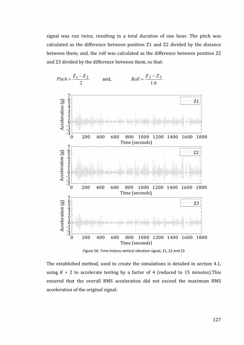
127
signal was run twice, resulting in a total duration of one hour. The pitch was
calculated as the difference between position Z1 and Z2 divided by the distance
between them; and, the roll was calculated as the difference between position Z2
and Z3 divided by the difference between them, so that:
2
21 Ζ−Ζ=Pitch and,
6.1
32 Ζ−Ζ=Roll
0 200 400 600 800 1000 1200 1400 1600 1800-3-2-101234567
Time (seconds)
Acc
eler
atio
n (
g)
0 200 400 600 800 1000 1200 1400 1600 1800-3-2-101234567
Time (seconds)
Acc
eler
atio
n (
g)
0 200 400 600 800 1000 1200 1400 1600 1800-3-2-101234567
Time (seconds)
Acc
eler
atio
n (
g)
Z3
Z2
Z1
Figure 56: Time history vertical vibration signal, Z1, Z2 and Z3
The established method, used to create the simulations is detailed in section 4.1,
using K = 2 to accelerate testing by a factor of 4 (reduced to 15 minutes).This
ensured that the overall RMS acceleration did not exceed the maximum RMS
acceleration of the original signal.

128
6.1.3 Measuring Product Damage
There are many mechanisms of damage for packaged-products e.g. scuffing,
denting or compressing, which can be described qualitatively, but cannot easily be
translated to a quantitative measure. To allow a more accurate evaluation of
different simulation techniques it is important to have a method of quantifying
product damage to remove subjectivity in the classification of the damage. For this
purpose the Equivalent Bruise Index (EBI) was used.
The EBI provides a method of doing this by classifying apple bruising by measuring
the diameter of bruises (Peleg, 1985). Thus, a numerical value can be given to the
level of specimen damage, which can then be used to compare the severity of
different simulation methods. This method was used in a previous study to
quantify damage to green Golden Delicious apples (Vursavus and Ozguven, 2004).
Using green rather than bi-coloured apples reduced the error in damage grading
(Leemans et al, 2002). In this study it is used on Granny Smith apples. To calculate
the EBI, the percentage of apples with bruising relating to each Degree of Damage
(DoD) is multiplied by the rating index (R) associated with that DoD shown in
Table 11.
∑=
=5
1
(%)l
l RDoDEBI (22)
where l equals 1 to 5, relating to the DoD’s given in Table 11.
Table 11: DoD classification and rating index (Peleg, 1985)
RATING
INDEX (R)
DEGREE OF
DAMAGE
(DoD)
SINGLE BRUISE
DIAMETER(mm)
EQUIVALENT DIAMETER OF
AGGREGATE BRUISES (mm)
0.0 None (1) 0.0 <12
0.1 Trace (2) <12 12 – 19
0.2 Slight (3) 12 – 19 19 – 25
0.7 Medium (4) 19 – 25 25 – 32
1.0 Severe (5) >25 >32

129
In addition to the EBI, the total area of bruising (Total Bruise Area (TBA)) for each
tray of apples is also determined.
6.1.4 Test Product Conditioning
The transport packaging used in this study was single walled corrugated trays
supplied by Riverford. Each case contains 42 apples. An example test tray can be
seen in Figure 57.
Figure 57: Riverford home delivery tray and load example, used during testing
Prior to testing, the apples were stored for 2 days in a room at ~16 deg C.
Afterwards, all apples were checked for bruising, the diameters of any bruises
were measured and the EBI was calculated for each tray. After testing all the trays
were stored for 5 days in a room at ~16 deg C, to allow any new bruising to
develop. After this time, each tray’s EBI was calculated. For each test a new tray of
42 apples weighing approximately 6 kg was used. For each of the six different
simulations three different packaging configurations were used: a single column
that is not shrink-wrapped; a single column of 5 trays shrink-wrapped (Figure 37);
and, 4 columns of 5 trays shrink-wrapped to simulate a unitized load. These three
packaging configurations were selected to provide insight into the effect that
different packaging configurations had on specimen response to MDOF vibration
and whether particular loading configurations may require MDOF testing.

130
Test specimen Test specimen
Figure 58: Single column unitized and four columns unitized
During testing, the test specimen was located within the uppermost layer of the
stack. Evidence from a previous study showed that the response of packaged
products to vibration is amplified upwards through the stack and that therefore
the top of the stack is subject to the most severe vibration (Berardinelli et al,
2004). All lower level trays were filled with 6 kg of potatoes to mimic the loading
of apples. In addition to the different stacking arrangements a test was undertaken
with a reduced number (eleven) of apples to simulate loose loading and therefore
simulate increased specimen movement. These trays were then packaged in the
same configuration as shown in Figure 57.
6.2 Results
The EBI calculated for each test tray is given in Table 12, where both the pre
testing and post testing EBI’s are stated. These were used to calculate the increase
in EBI. Similarly in Table 13, the pre testing Total Bruise Area (TBA), post testing
TBA and the increase in TBA are presented.
Throughout the different tests, the EBI varied from 19.2 for the SDOF time history
simulation to 56.9 for the MDOF Gaussian simulation.

131
The EBI calculated in Table 12 together with the TBA calculated in Table 13, are
presented in graphical form in Figure 59. This Figure shows the similarity between
the results using each method to calculate the damage.
Table 12: EBI calculation for different test regimes
TRAY
No CONFIGURATION TEST
PRE TEST
EBI
POST
TEST
EBI
INCREASE
IN EBI
1 Single Column –
Loose
SDOF time history 60.2 89.6 29.4
2 SDOF established
method 33.0 84.2 51.2
3
Single Column –
Shrink-wrapped
SDOF time history 39.8 66.6 26.8
4 SDOF established
method 51.6 101.8 50.2
5 MDOF time history 38.1 81.4 43.2
6 MDOF established
method 59.1 116.0 56.9
7
Four columns –
Unitized
SDOF time history 44.0 63.2 19.2
8 SDOF established
method 36.4 64.5 28.1
9 MDOF time history 34.1 64.3 30.2
10 MDOF established
method 31.8 88.2 56.4
Table 13: Total bruise area for test regimes
TRAY
No CONFIGURATION TEST
PRE TBA
(mm2)
POST
TBA
(mm2)
INCREASE
IN TBA
(mm2)
1 Single Column –
Loose
SDOF time history 5023 7225 2202
2 SDOF established
method 3079 6614 3535
3
Single Column –
Shrink-wrapped
SDOF time history 2697 4306 2488
4 SDOF established
method 3973 9278 5304
5 MDOF time history 3761 7797 4036
6 MDOF established
method 4731 10266 5536
7
Four columns –
Unitized
SDOF time history 2603 5091 1609
8 SDOF established
method 2818 4366 1548
9 MDOF time history 3367 6032 2665
10 MDOF established
method 2525 6916 4391

132
Figure 59: EBI and TBA (x103
mm2) for each simulation method and loading configuration
The EBI of the individual apples in tray 5 (MDOF time history) and tray 3 (SDOF
time history) is given in Figure 60 (a) and (b), respectively. There is a clear
variation in the apple EBI. This is due to their respective location within the tray,
with apples in the bottom layer suffering greater bruising than apples in the top
layer. To therefore get a clear overview of the bruising damage the EBI of all of the
apples within each tray is considered in order to reduce error in the calculation
that may arise due to the use of a sample of apples form each tray.

133
5 10 15 20 25 30 35 400
1
2
3
4
Apple number
EB
I
5 10 15 20 25 30 35 400
1
2
3
4
Apple number
EB
I
Mean EBI
EBI
Mean EBI
EBI
Figure 60: EBI for each apple for (a) tray 5 and (b) tray (3)
Because damage is being measured on a non uniform product, it is expected that
there will be error in the results, due to changes in the apple structure, firmness,
size, etc. Therefore, the results from this study can be used as a comparison of test
severity but cannot be used as an accurate measure of precise damage.
6.2.1 Comparison of the Different Packaging Configurations
The results show that by unitizing several columns of trays the level of product
damage is greatly reduced. This was true for the SDOF and MDOF time replication
and the SDOF established method. Application of the MDOF established method
produced high levels of damage in both configurations. This comparison is shown
in Table 14.
(a)
(b)

134
Table 14: Reduction in EBI between single column and unitized load configurations subjected to
various simulation methods
CONFIGURATION EBI SINGLE
COLUMN
EBI
UNITIZED
REDUCTION IN
EBI
Time History – SDOF 26.8 (3) 19.2 (7) 26%
Time History – MDOF 43.2 (5) 30.2 (9) 30%
Established method– SDOF 50.2 (4) 28.1 (8) 44%
Established method – MDOF 56.9 (6) 56.4 (10) 0%
6.2.2 Comparison of SDOF and MDOF Simulation
In addition to the variation of damage due to stack configurations, there is also a
sizeable increase in the level of damage recorded when using MDOF simulations in
comparison with those involving a SDOF. In both configurations single column and
unitized, the apples subjected to time history MDOF showed 60% more damage
(Table 15). The specimens subjected to SDOF and MDOF Gaussian simulations
varied from an increase of 13% for the single column to 100% increase for the four
column unitized load.
Table 15: Increase in EBI from real time and established method simulations using SDOF and MDOF
CONFIGURATION EBI FOR
SDOF
EBI FOR
MDOF
INCREASE
IN EBI
Time History - Single column unitized 26.8 (3) 43.2 (5) 61%
Established method - Single column unitized 50.2 (4) 56.9 (6) 13%
Time History - Four columns unitized 19.2 (7) 30.2 (9) 57%
Established Method - Four columns unitized 28.1 (8) 56.4 (10) 100%
6.2.3 Comparison of Time History and Gaussian Simulations
In general, the tests conducted using Gaussian signals tended to produce more
damage than those conducted using time history signals, with the variation
between the two being greatest when considering SDOF simulations.

135
Table 16: Comparison of EBI between time history and Gaussian simulations for a
single column
DEGREES OF
FREEDOM
EBI VARIATION
IN EBI TIME HISTORY GAUSSIAN
SDOF 26.8 (3) 50.2 (4) 87%
MDOF 43.2 (5) 56.9 (6) 32%
6.2.4 Comparison of Simulation Methods with Accelerated Testing
In comparison with the time history and the Gaussian simulations, the accelerated
tests produced significantly more specimen damage, as shown in Figure 61. It was
considered that this may be due to the test acceleration used i.e. time acceleration
of 4 and k = 2 create an over test.
0.0
20.0
40.0
60.0
80.0
100.0
120.0
140.0
Real time Gaussian Accelerated Gaussian
EBI
Figure 61: Comparison of the three different simulation techniques
To evaluate, additional testing was carried out where specimens were subjected to
two hours of time history simulation using SDOF and MDOF models. By then
comparing the time accelerated test results with those from the two hour test, the
test acceleration would be equivalent to a time acceleration of 8 and k = 3.
The results, of Table 17 show that with the increase in duration the damage also
increased to a level similar to that seen with the accelerated testing. This would
SDOF
MDOF
EB
I

136
suggest that a higher value of k is required for these apples. Therefore, these
results show some correlation in the use of accelerated Gaussian testing and actual
time history for specimen damage.
Table 17: Comparison of time history the simulations with the accelerated
Gaussian equivalent simulations
DEGREES OF
FREEDOM
TIME HISTORY EBI ACCELERATED
GAUSSIAN EBI 1 HOUR 2 HOUR
SDOF 26.8 (3) 62.5 89.5
MDOF 43.2 (5) 89.9 91.1
6.3 Discussion
Specimens placed in the more stable load of four unitized columns incurred
noticeably less damage. During testing, the single column configuration showed
visually more movement, with additional sway movement that had not occurred in
the more stable four column arrangement. Although there was additional
movement, the percentage increase in damage between the two packaging
configurations was similar.
There were three aims for the study, each of these is now defined and discussed.
1. Quantify and compare the damage caused to the test product under SDOF and
MDOF time replication simulation.
In both loading configurations the time replication simulation using MDOF
produced a significantly higher level of damage, with the EBI for the MDOF
increasing by 61% for the single column and 57% for the unitized load
configuration. This indicates that if time replication testing were used, a SDOF
approach would result in an under test of the packaging.
2. Using the results from the time replication tests, analyse the ability of the
established method to recreate damage, using both SDOF and MDOF testing.

137
When comparing the established method without test acceleration results
with the corresponding time replication tests it can be seen that the
established method produced an over test in all cases. On comparing the
results from the SDOF established method simulation to the MDOF time
replication simulation it can be seen that similar levels of damage were
recorded in both cases. Although the SDOF established method simulation
appears to produce additional damage not seen in the SDOF time history, it
does tend to produce a comparative level of damage to what would be caused
by the actual vehicle movement (MDOF time history).
3. Evaluate the use of the established method with test acceleration, using both
SDOF and MDOF simulations, to recreate MDOF damage.
Initial testing, using the established method with test acceleration of 4 and k =
2, showed that, on average, more damage occurred than when using the MDOF
time replication. Thus it provided a severe over test. However, when
comparing the damage with that produced from the time history simulations
of a longer duration (two hours instead of one hour) with corresponding test
acceleration of 8 and k = 3, the damage produced by both the SDOF and MDOF
accelerated Gaussian signals was similar to that of the MDOF time history.
6.4 Concluding Remarks
From the testing it can be concluded that the MDOF simulation produced more
damage than the SDOF, in all cases. This suggests that simulating only the vertical
vibration of the vehicle provides a significant under test. What is also interesting to
note is that the SDOF established method simulated a similar level of product
damage to that of the MDOF time history simulation in both load configurations.
Furthermore, the significance of MDOF vibration was found to be dependent on
packaging configuration, with a less stable configuration being most affected by the
MDOF movement. The results from this testing suggest that when designed

138
correctly, a single axis vibration simulation can represent MDOF vibration of a
distribution vehicle.
This study also indicated that the degree of test acceleration and the value of k are
product dependent. Therefore, in order to carry out test acceleration with
confidence the appropriate acceleration and value of k must be known. However,
establishing the correct value of k for a particular packaged product would require
significant test time and evaluation.
Therefore, the improved simulation approach presented in this Thesis will be
designed, at present, for SDOF vertical axis application without test acceleration.
It is noted that as testing was carried out on a single product, the results cannot be
directly transferred for all products, though it does provide a good guide. In the
case of food and drink distribution, where products are packaged in a more
protective manner than the apples used in this study, thereby minimising the
movement between products, the additional damage caused by movement in axes
other than the vertical would be greatly reduced by comparison.

139
7 TIME-FREQUENCY ANALYSIS
Analysing a non-stationary and non-Gaussian vibration signal using only a
frequency domain technique, such as Fourier transforms, does not account for the
events within the signal that make it non-stationary or non-Gaussian. Rather, it will
represent the signal as an average. Consequently, any simulation produced based
on this information, will be stationary and have a Gaussian distribution. Thus, it
will not be representative of the true nature of vehicle vibration. This leads to
errors in the simulation and a need for conservatism in packaging design to
account for this.
By using an analysis technique that identifies and illustrates changes in the
frequency domain with respect to time, features characteristic of a signal’s non-
stationary and non-Gaussian nature can be detected. Three techniques: Short Term
Fourier Transform (STFT); the continuous wavelet transform (CWT); and, the
discrete wavelet transform (DWT) are discussed.
7.1 Short Term Fourier Transform (STFT)
The STFT, also known as the Gabor Transform, applies the DFT to continuous
sections of a signal, allowing that signal’s frequency content to be analyzed over
localities in time. The equation for the STFT is given by:
{ } dtetwtxXtxSTFT ti
mωτωτ −∞
∞−−=≡ ∫ )()(),()( (23)
where X(τ, ω) is the Short term Fourier Transform for the series of windowed
function, x(t)w(t - τ), of the subject function, x(t), at a localized time point, τm = mτo
where τo is the time spacing between successive DFT calculations and m is an
integer 1 to the number of DFT calculations required, this is dependent on the
length of x(t). The Fourier Transform of the windowed function for τ and ω is then
determined.

140
When the STFT is used in this Thesis a rectangular window of length N is used,
which surrounds the time point τ. An example of the application of the rectangular
window is given in Figure 62 (a) to (d), in this example N is equivalent to one
second and there is zero overlap between windowed function. The rectangular
window in (b) is applied to the function x(t) in (a), the resulting windowed
functions for τ1 and τ2 are then given in (c) and (d), respectively.
0 1 2 3 4 5 6 7 8 9 10-1
-0.5
0
0.5
1
Time (seconds)
Acc
eler
atio
n (
g)
0 1 2 3 4 5 6 7 8 9 100
1
Time (seconds)
Acc
eler
atio
n (
g)
τ1 τ2
0 1 2 3 4 5 6 7 8 9 10-1
-0.5
0
0.5
1
Time (seconds)
Acc
eler
atio
n (
g)
0 1 2 3 4 5 6 7 8 9 10-1
-0.5
0
0.5
1
Time (seconds)
Acc
eler
atio
n (
g)
0.5
x(t)w(t-τ2)
x(t)w(t-τ1)
Rectangular window
x(t)
Figure 62: Example application of the rectangular window for the STFT
The temporal resolution afforded by the STFT means that variations in the
frequency domain can be seen over time. Although the technique uses a stationary
(a)
(b)
(c)
(d)

141
signal processing method, because of the sliding window the overall technique is
non-stationary (Akansu and Haddad, 2001).
Gabor (1945) observed that ‘...although we can carry out the analysis with any
degree of accuracy in the time direction or in the frequency direction, we cannot
carry it out simultaneously in both beyond a certain limit’.
The limitation of this is that a compromise between time and frequency resolution
is required (Mallat, 1999). Therefore, in order to improve frequency resolution, the
time over which the frequency content is calculated needs to be increased, leading
to a reduction in the temporal resolution and vice versa. This relationship exists
for all transforms. However, the STFT has the additional limitation that the
resolution is fixed throughout the signals frequency range. For vehicle vibration,
where the predominant frequencies are low, having high frequency resolution at
low frequencies is important. Additionally, discrete transient events, also prevalent
in vehicle vibration, mean that high frequency events tend to occur over short-time
periods and therefore high temporal resolution is required at high frequencies.
Although the STFT allows for some improvement in the representation of vehicle
vibrations, it is of limited use. To ensure all events are captured correctly, a
transform that allows resolution variation is required.
7.2 Wavelet Analysis
Daubechies (1992) states that ‘the wavelet transform is a tool that cuts up data,
functions or operators into different frequency components, and then studies each
component with a resolution matched to its scale’.
Wavelet analysis is used in many applications because of its effectiveness when
detecting variations in signals. It is used in the decomposition of both
electrocephalagraph (EEG) and electrocardiogram (ECG) signals to identify
transients with respect to both the time and frequency domain (Adeli et al, 2003;
Sahambi, 1997). Further applications include fault diagnostics in mechanical

142
machinery and crack identification in structures (Liew and Wang, 1998; Jing and
Liangsheng, 2000).
Wavelet analysis enables the identification of a signal’s frequency content with
respect to time. It does this by continually comparing the signal to a number of
wavelet functions of varying length and frequency. The correlation between the
function and the signal is then expressed through a coefficient. The higher the
value of the coefficient, the better is the correlation between the signal and the
function at the given frequency.
The wavelet functions are all formed from a single base mother wavelet (ψ(t)). The
variation in the time frame (length) and frequency of the wavelet functions is then
obtained by expanding and compressing this mother wavelet.
Common mother wavelets include: Daubechies db2, db6 and db10 (Daubechies,
1990), where the numerical value refers to the number of vanishing moments;
Haar; Morlet; and, Mexican Hat, each of which are real or complex functions. These
mother wavelets are illustrated in Figure 63 (Addison, 2002).

143
0 1 2 3-2
-1
0
1
2db2 Wavelet
0 5 10
-1
-0.5
0
0.5
1
db6 Wavelet
0 5 10 15
-1
-0.5
0
0.5
1db10 Wavelet
-10 -5 0 5 10-1
-0.5
0
0.5
1Morlet Wavelet
0 0.5 1-2
-1
0
1
2Haar Wavelet
-10 -5 0 5 10-0.5
0
0.5
1Mexican Hat Wavelet
Figure 63: Mother wavelet functions
The degree of expansion or compression of the mother wavelet is determined by a
scaling parameter, a, which is inversely proportional to the frequency. A
translation parameter, b, then determines the location (time) of the analysis. So
that the wavelet function with translation, b, and scaling parameter, a (ψa,b(t)) can
be defined as:
−=
a
bt
atba ψψ
||
1)(, (24)
The term a-1/2 normalises the energy within the wavelet across the different
scales, keeping the energy of each wavelet function ψa,b(t) equal to that of the
mother wavelet function ψ(t).
Examples of a compressed wavelet, and an expanded wavelet, being compared to a
vibration signal are given in Figure 64. The scale (a1) of the compressed wavelet is
lower than the scale (a2) of the expanded wavelet. Additionally, they both have
different translation parameters (b1 and b2).

144
-0.5
0
0.5
1
Expanded wavelet (a2) Compressed wavelet (a1) a1 < a2
0 50 100 150 200 250 300 350 400 450 500-1
Position (b1) Position (b2)
Window length, L2 Window length, L1
Figure 64:Examples of a compressed and an expanded wavelet, with different translation parameters
In Figure 64, it is apparent that the expanded wavelet’s window length (L2) is
much larger than that of the compressed wavelet (L1). This means that the
expanded wavelet will carry out analysis over a larger time frame and will
therefore have a lower temporal resolution than that of the compressed wavelet.
This compression and expansion of the wavelet allows the resolution of the
analysis to vary. This is a benefit of wavelet analysis over STFT, as it enables a
lower frequency resolution but a higher temporal resolution when analysing high
frequencies (low scales), and conversely, it affords a higher frequency resolution
but lower temporal resolution at low frequencies (high scales).
This property of wavelets is useful when analysing signals such as vehicle
vibration, where low frequency vibration tends to be predominant and continual
throughout the signal, while high frequency events tend to occur over short
durations. This change in resolution and how it relates to the time and frequency
resolution has been expressed in Figure 65. In the figure it is apparent that as the
frequency of the wavelet increases, the scale (a) and the frequency resolution
decreases, but the time resolution increases.

145
Fre
qu
en
cy
Time
To analyse high frequencies the wavelet com-
presses, reducing the time over which the
analysis is carried out and hence increasing
the time resolution at high frequencies W
av
ele
t co
mp
ress
ion
—S
cale
(a
) d
ecr
ease
s
low frequency resolution and
high time resolution. When ana-
lysing high frequency informa-
tion.
High frequency resolution and low
time resolution. When analysing
low frequency information.
Figure 65: Wavelet analysis time and frequency resolution
7.2.1 The Continuous Wavelet Transform (CWT)
When using a real wavelet function, the continuous wavelet transform (CWT) is
found by calculating the convolution of the complex conjugate of the wavelet
transform (ψa,b(t)) and the time domain signal (x(t)) using the equation:
( ) ( ) ( ) ( ) ( )dtttxa
dta
bttx
aabCabCWT bax ∫∫
∞∞−
∞∞−
=
−=≡ ,
11,, ψψψ (25)
Where C(b,a) is the wavelet coefficient at position b and scale a. Typically a
discretised version of the CWT is used:
( ) ( ) ( )∑ ∑= =
−=≡
S
a
L
bx
a
bttx
aabCabCWT
1 1
1,, ψψ
(26)

146
where the wavelet coefficients are calculated for a number of scales a = 1,2,3,..., S, at
positions b = 1,2,3,..., L, where S is a limiting number of scales and L is the length of
the signal.
Note that if the wavelet function is complex, then the wavelet coefficients are found
as the convolution of the time domain signal with the complex conjugate of the
wavelet function.
The wavelet coefficients for an example vibration signal are illustrated in Figure
66. The real Morlet mother function, which is discussed later in this chapter, has
been used in the CWT equation (Equation 25) to calculate the absolute wavelet
coefficients. Where scales, a, used are all integer values from 1 to 128 and
positions b, are all integer values from 1 to 4100, where one second is equivalent
to 1500 data points. Changes in coefficients have been identified, a description of
the events within the signal they relate to and the information they provide the
user, has been given.
From Figure 66 the variation in the signal’s frequency content throughout the
range of scales can be seen. With low frequency components being present
throughout the length of the signal and higher frequency events tending to only
appear for short time frames. Shock events within the signal are clearly seen
within the wavelet analysis as high value coefficients.

0 500 1000 1500 2000 2500 3000 3500 4000-1
-0.75-0.5
-0.250
0.250.5
0.751
Time (seconds)
Acc
eler
atio
n (
g)
time (or space) b
scal
es a
500 1000 1500 2000 2500 3000 3500 4000 1
8
15
22
29
36
43
50
57
64
71
78
85
92
99
106
113
120
127
50
100
150
200
Position (b)
Position (b)
2
1.5
1
0.5
Ab
solu
te c
oef
fici
en
t v
alu
e C
(b,a
)
Scal
e (a
) A
ccel
erat
ion
(g
)
Areas of high accel-
eration in the signal are identified by high value coefficients at
the frequencies which are present
Higher value coeffi-
cients at low scales indicate high fre-quency content
Fre
qu
en
cy (
Hz)
Low
High
Time (seconds) = bΔt
Frequency (Hz) = central frequency (ωo)/(aΔt)
Areas where the coefficients are relatively similar indicate vibration that is relatively stationary with similar a frequency content.
Figure 66: Example of wavelet coefficients and how they are used to indicate changes within the vibration signal

148
7.2.2 Selecting a Mother Wavelet Function
As there are many mother wavelet functions the most appropriate one for use with
vehicle vibration signal analysis needs to be selected. To examine the variation
between the different wavelet mother functions, CWT has been used to analyse a
vehicle vibration signal, using the mother functions illustrated in Figure 63. The
vehicle vibration used is taken from part of a journey recorded on the Ford Luton
home delivery vehicle. The results from the different analyses are displayed in
Figure 67 and Figure 68. These demonstrate the variation in the appropriateness
of the different wavelet mother functions, for identify different features within a
signal. The results show quite clearly that both Daubechie’s db10 and, the Morlet
mother function, are the most suitable for analysing the vibration signal as they
detect the variations in frequency content more precisely. The Haar, Mexican hat
and Daubechie’s db2 mother functions, do not illustrate the variation in the
frequency content at each position clearly. Indicating that when considering using
a CWT within a new simulation technique either: Daubechie’s db10; db6; or, the
Morlet mother function should be used.

149
Figure 67: (a-c) Comparison of Wavelet Transforms

150
Figure 68: (d-f) Comparison of Wavelet Transforms

151
In order to identify and capture features within a signal using wavelet analysis, the
mother wavelet selected should identify the key features of the signal being
analysed.
Nei et al (2008) states that the Morlet function has relatively high performance for
both time and frequency resolution. Because in this application wavelet analysis is
being used to identify short duration transients in the signals, high resolution in
the time domain is important. Furthermore, Lin (2001) successfully used the
Morlet wavelet to identify impulses within a signal. A key feature of vehicle
vibration is discrete high level shock events (similar to impulses), and, in Figure
67, the Morlet transform managed to clearly identify variations in the frequency
content of the example vehicle vibration signal. Therefore the Morlet transform is
appropriate for use in this study.
The Morlet function is a complex wavelet, its equation is given by:
−−
−=2
24
22
1)(
t
tieeet
o
o
ωω
πψ (27)
Where ωo is the central frequency of the mother wavelet and the second term in
the brackets is the correction term, this corrects for the non-zero mean of the
complex sinusoid of the first term. From Equation 27 it can be seen that the Morlet
wavelet is a complex wave (e-iωt) masked by a Gaussian envelope (e-t^2/2).
When using the Morlet wavelet to analyse real signals, such as vehicle vibration,
only the real part of the Morlet wavelet is required (Tang et al, 2010). The equation
for the real Morlet wavelet is:
)cos(
1)( 2
2
4tet o
t
ωπ
ψ−
=
(28)
where ω0 ≥ 5. This is because when ω0 is greater than or equal to 5 the error in the
mean from zero is negligible and therefore the correction term in Equation 27 is no

152
longer required. From this point, when referring to the Morlet wavelet, the real
Morlet wavelet is being considered.
7.2.3 The Discrete Wavelet Transform (DWT)
Whilst the CWT affords many advantages, it also suffers some limitations. In
particular Akansu and Haddad (2001) state that, ‘…the continuous wavelet
transform suffers from two drawbacks: redundancy and impracticality’. The
redundancy issue arises from the overlapping of data when using the CWT and the
extensive computation time and power make the CWT impractical in many
situations. The Discrete Wavelet Transform (DWT) addresses these issues by
sampling the CWT scales (a), thereby reducing the number of scales and hence
reducing the computing time and removing redundancy. The scale (a) and
translation (b) parameters then become j
oaa −= and o
j
o kbab −= , respectively,
where j = 1,2,3,..., J and k = 1,2,3,..., K and a > 1 and b > 0:
( ) ( )oj
o
j
okj kbtaat −= ψψ 2/
, (29)
For the DWT the ao = 2 and bo = 1. This gives the equation for calculating the DWT
as:
( ) ( ) ( ) ( )dttxktkDWTbaDWT jjjj ∫+∞
∞−−− −== 222,2, ψ (30)
The signal is then decomposed into J levels. At each level the DWT separates the
signal into two parts using a high pass and low pass filter. A high pass filter retains
frequency information above the cut off frequency, fc and attenuates frequency
information below fc. Conversely, the low pass filter retains the frequency
information below fc and attenuates frequency information above fc. The cut off
frequency, fc = fs/2j, where fs = 1/Δt, and is the signal’s sampling frequency.
When using the DWT, at each level (j) the result from the high pass filter is stored
and the result from the low pass filter is then filtered further. The process
continues until the limiting number of levels (J) is reached, this filtering process is
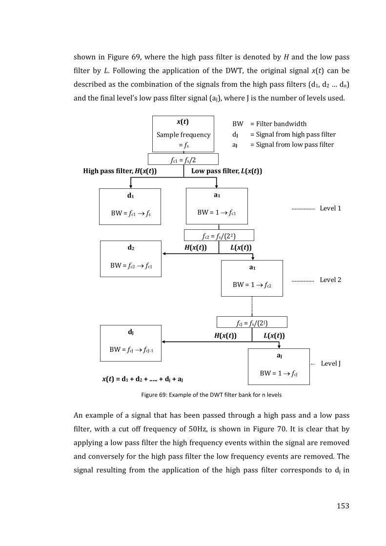
153
shown in Figure 69, where the high pass filter is denoted by H and the low pass
filter by L. Following the application of the DWT, the original signal x(t) can be
described as the combination of the signals from the high pass filters (d1, d2 … dn)
and the final level’s low pass filter signal (aJ), where J is the number of levels used.
High pass filter, H(x(t))
d1
Low pass filter, L(x(t))
x(t)
Sample frequency
= fs
fc1 = fs/2
BW = fc1 → fs
H(x(t)) L(x(t))
fc2 = fs/(22)
H(x(t)) L(x(t))
fcJ = fs/(2J)
Level 1
Level 2
Level J
a1
BW = 1 → fc1
d2
BW = fc2 → fc1 a1
BW = 1 → fc2
dJ
BW = fcJ → fcJ-1 aJ
BW = 1 → fcJ
BW = Filter bandwidth
dJ = Signal from high pass filter
aJ = Signal from low pass filter
x(t) = d1 + d2 + ..... + dj + aJ
Figure 69: Example of the DWT filter bank for n levels
An example of a signal that has been passed through a high pass and a low pass
filter, with a cut off frequency of 50Hz, is shown in Figure 70. It is clear that by
applying a low pass filter the high frequency events within the signal are removed
and conversely for the high pass filter the low frequency events are removed. The
signal resulting from the application of the high pass filter corresponds to dj in

154
Figure 69 and the signal resulting from the application of the low pass filter
corresponds to aj.
0 0.2 0.4 0.6 0.8 1 1.2 1.4 1.6 1.8 2-0.4
-0.2
0
0.2
0.4
Time (seconds)
Acc
eler
atio
n (
g)
0 0.2 0.4 0.6 0.8 1 1.2 1.4 1.6 1.8 2-0.4
-0.2
0
0.2
0.4
Time (seconds)
Acc
eler
atio
n (
g)
0 0.2 0.4 0.6 0.8 1 1.2 1.4 1.6 1.8 2-0.4
-0.2
0
0.2
0.4
Time (seconds)
Acc
eler
atio
n (
g)
Highpass filter @ 50Hz
Lowpass filter @ 50Hz
Signal 1-250Hz
Figure 70: Example use of low pass and high pass filters with a cut off frequency of 50Hz
Nei et al (2008) used the discrete wavelet transform (DWT) with J = 8, to create a
method of shock superposition for vibration testing, thus an 8 level DWT was
carried out. The study found that the signal’s discrete shock events were visible
within levels 3 – 5. It was therefore recommended that when creating a simulation
signal, short time segments within the signal should be amplified within the
frequency range covered in levels 3 - 5, enabling a more accurate representation of
both the amplitude and frequency variations throughout the signal. It was also
recommended that the location and frequency of these amplified events, within the
signal, be determined by their appearance and positioning within actual vehicle
vibration.

155
7.3 Comparison of Time-Frequency Analysis Techniques
The signal in Figure 71 has been used to compare STFT, CWT and DWT analysis
techniques. The signal was recorded in an empty Ford Luton box van during a
home delivery journey in the city of Bath, UK. It has a sample time of 0.000585
seconds and has been passed through a band pass filter of range 1 - 250 Hz.
The STFT analysis of the signal is displayed in Figure 72. This was calculated using
the following properties:
• Size of FFT: 211
• STFT Segment size: 211
• Sample frequency: 1710 Hz
• Overlap of segments: 0
0 10 20 30 40 50 60-2
-1
0
1
2
Time (seconds)
Acc
ele
rati
on
(g
)
Figure 71: Example vehicle vibration signal to carry out comparison of time-frequency analysis
techniques
The CWT and the DWT evaluations are displayed in Figure 73 and Figure 74,
respectively. These analyses were carried out using the Matlab Wavelet Toolbox.
The CWT was undertaken using the Morlet mother function and 128 scales, whilst
the DWT was carried out using the Daubechies db6 mother wavelet function and
was decomposed to 12 levels.

156
10 20 30 40 500
200
400
600
800
Time (seconds)
Fre
qu
ency
(H
z)
0 10 20 30 40 50 60-2
0
2
Time (seconds)
Acc
eler
ati
on
(g)
-140
-120
-100
-80
-60
-40
-20
Figure 72: STFT of the signal given in Figure 71
Scale of colors from MIN to MAX
Position (b)
Sca
le (
a)
1 8
15 22 29 36 43 50 57 64 71 78 85 92 99
106113120127
0 10 20 30 40 50 60-2
0
2
0
2
-2
0
10 20 30 40 50 60 Time (seconds)
Figure 73: CWT of signal given in Figure 71 using the Morlet transform

157
-0.5-0.25
00.25
0.5d10
0.5
-2-1.5
-1-0.5
00.5
11.5
2s
-0.5-0.25
-00.25
0.5d1
-0.5-0.25
00.25
0.5d2
-0.5-0.25
00.25
0.5d3
2 4 6 8
x 104
-0.5-0.25
00.25
0.5d4
-0.5-0.25
00.25
0.5d5
-0.5-0.25
00.25
0.5d6
0.52 4 6 8
x 104
-0.5
-0.5-0.25
00.25
0.5d7
-0.5-0.25
00.25
0.5d8
-0.5
2 4 6 8-0.5
-0.250
0.250.5
d9
-0.5
-0.5-0.25
00.25
0.5d11
-0.5-0.25
00.25
0.5d12
2 4 6 8
x 104
-0.5-0.25
00.25
0.5a12
Figure 74: DWT of signal given in Figure 71 using Daubechie db6
By analysing vehicle vibration using a time-frequency technique it is possible to
identify variations in the signal’s intensity and frequency content over time. This
allows for transients within the signal to be identified. In both Figure 72 and Figure
73, the high acceleration transient events, present in the signal in Figure 71 at
approximately 47 and 58 seconds, are quite clearly visible. This is particularly true
when considering the result from the continuous wavelet analysis, where high
value coefficients are visible at these time points, throughout the full range of
scales (1 to 128).
The DWT benefits from a reduced requirement of computational time and
capabilities when compared with the CWT. This makes the DWT useful when
evaluating vehicle vibration. Unfortunately, the DWT does suffer from some
limitations. Firstly, the frequency resolution of the DWT is much lower than that of

158
the CWT due to the reduced number of levels used. Therefore, by using the CWT a
more detailed view of the frequency variations in the signal can be obtained.
7.4 Concluding Remarks
The ability of time-frequency analysis techniques to identify transients and varying
frequency content in vehicle vibration has been presented. It has been shown that
whilst the STFT identifies variation in the signal, it is limited in resolution. This
prevents it from fully recognising the short-time transient events present in
vehicle vibration and also the accurate variation in frequency content variation. In
contrast, the varying time and frequency resolution afforded by the CWT enables
these events to be more accurately described.
The use of CWT is desirable in the analysis of non-stationary and non-Gaussian
signals, such as vehicle vibration. Whilst the CWT is appropriate for analysing the
signal and identifying variations in the frequency content and amplitude, its use
within an approach for simulating vehicle vibration, is not so straight forward. This
is mainly due to the way in which it analyses the signal. When inverting the CWT
the original time history signal is returned, this therefore presents no obvious way
in which several vibration signals can be considered in parallel to create an
average representative simulation. Additionally it does not allow for the signal to
be represented in a manner that is useable on most simulation rigs.
Vehicle vibration is unpredictable and highly unrepeatable. A key benefit of the
established method is that it lends itself to journey averaging, enabling the
inclusion of data from several journeys, giving the resulting simulation statistical
significance. Additionally, this method also lent itself to application on existing
laboratory simulation controllers, and, facilitated test acceleration. It is therefore
apparent that while the CWT alone cannot be used to form a simulation approach,
it can be used in conjunction with the established method to create a more suitable
simulation approach.

159
Because of this, a new approach of simulating vehicle vibration, that utilises the
CWT, has been developed.

160
8 A TIME-FREQUENCY APPROACH FOR
SIMULATING VEHICLE VIBRATION
It is apparent that in order to identify signal transients when analyzing a non-
stationary and non-Gaussian signal, a time-frequency analysis method should be
adopted. In section 7.3, it was recognized that time-frequency wavelet analysis,
provides the most suitable method for identifying these signal transients.
In section 4 the RMS modulation approach, developed by (Rouillard and Sek,
2010), was evaluated. A random non-stationary vehicle vibration can be described
as a sequence of zero-mean Gaussian segments. This allows the signal to be defined
by a series of RMS acceleration levels and ‘vibration doses’ (durations) (Rouillard,
2007a). The resulting simulation has a varying RMS acceleration characterized by
a given statistical distribution. This method evolved from previous work, which
evaluated the non-stationary and non-Gaussian characteristics of vehicle vibration,
with particular attention to the statistical content of vehicle vibration signals
(Rouillard, 2007a; Rouillard and Sek, 2000).
In the correlation study, presented in section 5, the RMS modulation method was
shown to correlate well with vertical vibration time replication, producing only a
small error (5% under test), when considering the damage mechanism of scuffing.
As the RMS acceleration varies the signal’s average PSD is uniformly scaled.
Therefore while the method simulates the RMS acceleration distribution of a signal
it does not account for variations in frequency content. By not accounting for the
change in frequency content at different RMS acceleration levels, important
frequency responses seen in time replication may be missed and this therefore
may be a source of error.
It has been concluded, that by creating a simulation approach that analyzes the
change in spectral shape along with the RMS acceleration distribution, a more

161
accurate representation of vehicle vibration can be formed. In order to analyse the
change in spectral shape over time a time-frequency analysis tool based on the
wavelet transform may be used.
Because the CWT retains the signal’s information, when inversed it reproduces the
original time-domain signal. Because of this, used independently, it only presents a
more appropriate method of analyzing a signal to identify transient events.
Therefore, it does not offer a suitable method of producing a simulation which is
both usable on existing controllers and is statistically significant e.g. create a
simulation from multiple and averaged data so that it contains events that are
likely to occur in real life. This limitation, along with consideration of the work
carried out by Rouillard and Sek (2010), has led to the construction of a simulation
approach which employs a combination of time-frequency and frequency analysis
tools.
The method presented uses an iterative approach to decompose a non-stationary
signal, with a non-Gaussian distribution, in to approximately stationary and
Gaussian parts of varying amplitude and duration. Each of these parts can be
represented as a PSD and duration. By then applying these parts at random, a
simulation signal, that has a similar RMS acceleration distribution, kurtosis, and
average PSD to the original signal, can be formed. By incorporating the use of
frequency analysis, the resulting simulation is usable on existing laboratory
controllers, and has the potential for both signal averaging and test acceleration, if
required.
A detailed explanation of the development of the wavelet decomposition method is
now given, followed by a worked example of the method.

162
8.1 The Wavelet Decomposition Method for Simulating
Vehicle Vibration
The wavelet decomposition method involves a two-level iterative approach. At
each stage wavelet analysis is used to decompose a vibration signal into two parts:
that which falls within a Gaussian envelope (low level vibration) and that which
exceeds the Gaussian envelope (high level vibration). These two parts are referred
to respectively, as the Gaussian approximation and the non-Gaussian part.
On the first iteration the original vibration signal is decomposed, on proceeding
iterations, the non-Gaussian part resulting from the previous iteration is then
decomposed.
Once a limiting number of iterations M have occurred, or the non-Gaussian part
produced has a kurtosis below an acceptable value, the first level of iterations
stops and the final non-Gaussian part becomes the M+1th Gaussian approximation.
In order to then refine each of the Gaussian approximations, the distribution of
each (1 to M+1) is evaluated. If an approximation’s kurtosis is above an acceptable
value, a second level of iteration takes place. This second level of iteration is used
to reduce the size of the signal parts, enabling the creation of smaller more
stationary parts with distributions closer to Gaussian.
At the end of the iterative process, the signal has been decomposed in to a number
of parts that have approximately Gaussian distributions, which when
reconstructed together would reform the original vibration signal.
Because each part is approximately stationary with an approximately Gaussian
distribution, they can each be defined relatively accurately by their PSD and
duration. A simulation signal can then be created by randomly simulating each
part. When simulated together, the parts form a simulation signal that is non-
stationary and non-Gaussian with the same average PSD, average RMS acceleration
and duration as the original signal.

163
A flow diagram illustrating the wavelet decomposition method is given in Figure
75. A detailed explanation of each step is then given.

164
YES
NO
NO
Calculate the PSD
and RMS for the
Gaussian segment
If m < M
Non-Gaussian =
Vibration Signal
m+1
Else
Non-Gaussian =
Gaussian M+1
Separate signal ‘Gaussian, m’
and ‘non-Gaussian, m’
‘Gaussian’ part
Measure the kurtosis
Kurtosis, k <= accept-
able level?
Calculate the PSD
and RMS for the
Gaussian segment
Find outlying
segments
Wavelet analysis of
vibration signal
Vibration Signal m Where : m = 1,2,...,M
Calculate the PSD of
the vibration signal Construct Gaussian
equivalent signal
Wavelet analysis of
Gaussian equivalent
signal
Build envelope of
max and min
Gaussian scales
LEVEL1
LEVEL 2
1 2
3 3
4
6
7
8
9
9
5
Repeat steps 1-8 For s = 1,2,3,...,S
For each ‘Gaussian’
part m = 1-M
‘non-Gaussian’
part
Measure the
kurtosis
Kurtosis, k <= ac-
ceptable level?
m = m+1
YES
Non-Gaussian m = Gaussian m+1
M = m
Apply each PSD
at random for the
corresponding
duration creating
a simulation
signal
10
Simulated signal
0 100 200 300 400 500 600-1.5
-1
-0.5
0
0.5
1
1.5
Time (seconds)
Acc
ele
rati
on
(g)
Figure 75: Flow chart illustrating the process of decomposing vibration signal using wavelet analysis

165
Matlab has been used to construct a code for creating simulations using the
wavelet decomposition method. The associated code is included in Appendix V.
In the first level of iteration (Figure 75) M iterations take place, where m = 1, 2, 3,
… M, represents the current iteration number. The value of M is decided by one of
two factors, either:
1. M = a limiting number of iterations, e.g. a maximum 3 iterations are
carried out.
2. Or, M = the number of iterations until the high level vibration part, that
exceeds the Gaussian envelope, has k <= the acceptable limit.
Step 1 of the wavelet decomposition method calculates the average PSD (Sm(f)) for
the vibration signal. When:
• For the first iteration (m = 1), the vibration signal, y1(t) = original vibration
signal
• For any subsequent iterations (1 < m ≤ M), the vibration signal, ym(t) = the
non-Gaussian part, yNGm-1(t).
The average Fourier spectrum, Ym(f), can be calculated using an adaption of
Equation 12. In order to find the DFT, Ym(fk), of a non-periodic signal, ym(t), the DFT
would need to be calculated over the entire signal so that the sample size N would
be equal to the length of the signal. To therefore reduce the size of the DFT, an
average DFT for the signal is calculated. This is done by calculating the DFT for
each segment of the signal (length N data points) as it falls within a window. In
order to get the most accurate average, windowed segments should overlap by N-1
data points, giving the equation:
∑ ∑−
=
−
=
−+=1
0
1
0
)2()(
1)(
Q
q
N
r
rtkfieqtrtmy
QkfmY
π (31)
where:

166
fk = kΔf, DFT frequency (Hz)
k = 0, 1, 2, ..., N
tNf
∆=∆
1, frequency bandwidth (Hz)
ym(tr + tq) is the input signal at position (tr + tq).
tr = rΔt= 0, 1, 2, ..., N-1
tq = qΔt = 0, 1, 2, ... Q-1, the time point to move sampling window to.
Q = Number of data points in the signal (ym(t)) – (N-1) = number of signal
segments of length N averaged to form the average DFT. (N-1) is the overlap of
segments used.
Because of aliasing of frequencies above the Nyquist frequency, fN (as discussed in
section 3.1.9), the DFT frequency, fk represents the frequencies:
>
∆
−∆
≤∆=
2
12N
kHzttN
k
NkHz
tN
k
fk
To remove the negative frequencies the Fourier spectrum Ym(f), has been
truncated after the (N/2)th value, creating a one-sided spectrum of only positive
frequencies.
The average PSD is then calculated from the average Fourier spectrum (Garcia-
Romeu-Martinez, 2008):
2)(
2)( fY
N
tfS my
∆=
(32)
Where Ym(f) is now the one sided Fourier spectrum and the multiplication of 2
compensates for using the one-sided spectrum of length N/2.

167
Step 2 creates a signal from the PSD, Sy(f), this signal has the same average PSD,
overall RMS acceleration and duration as the vibration signal. But because the
signal is constructed from average data, it will ultimately be stationary (it will have
a constant RMS acceleration), and it will have a Gaussian distribution. Therefore
the simulation signal produced from the PSD will have the same average frequency
distribution as the original signal and the same overall RMS acceleration, but it will
not recreate the non-stationary nature and the non-Gaussian distribution of the
original vehicle vibration. Hence why a signal simulated from the PSD is referred to
in this Thesis as the equivalent Gaussian signal.
A Gaussian signal is created by inverting Equation 32 and utilising Equation 13 for
the inverse DFT. Firstly, the PSD is inverted giving the one sided Fourier spectrum:
iPye
t
NfSfXOnesided
∆=
2
)())((
(33)
Because when calculating the PSD, the signal’s phase information is lost, a random
phase, between 0 and 2π must be added to form the complex one sided Fourier
spectrum (X(f)).
jPhaseefXfXOnesided )())(( = (34)
Where:
Phase = a random phase array.
The two sided DFT (Xm(f)), is then constructed by concatenating the one sided
Fourier spectrum with its complex conjugate (X*(f)) .
A time domain signal segment of time length NΔt can then be constructed by
applying the inverse DFT.

168
In order to then obtain a time domain signal with the same duration as the original
vibration signal (ym(t)), L, the process in step two needs to be repeated n times,
where:
tN
Ln
∆=
The resulting n signal segments are concatenated to form a time domain signal
xm(t), of duration L, the same duration as ym(t). An example of a vibration signal
and its equivalent Gaussian signal is given in Figure 76.
0 100 200 300 400 500 600-2
-1
0
1
2
3
Time (seconds)
Acc
eler
atio
n (
g)
Gaussian Equivalent
Original Signal
Figure 76: Comparison of original signal and its Gaussian equivalent
Step 3, wavelet analysis is performed on both the vibration signal and the
equivalent constructed signal. The CWT (Equation 25) is used with the Morlet
mother wavelet function, ψ defined by Equation 28, to calculate the wavelet
coefficients of both signals, Xm(t) and Ym(t).
( ) ( ) dta
bttx
aabX mm
−= ∫ ψ
1,
(35)
A ‘Gaussian’ envelope is then constructed from the maximum and minimum
coefficient values at each scale (a) of the constructed signal’s wavelet coefficients:
)),(max()( iBXiMax m=
)),(min()( iBXiMin m=

169
where:
i = 1, 2, …, A
A is the total number of scales
B = all positions, b.
An example of the Gaussian envelope is given in Figure 77. In Step 4, this envelope
is compared with the vibrations signal’s wavelet coefficients for all positions (b),
and in Step 5 any coefficients that exceed the Gaussian envelope’s maximum or
minimum values are identified, these coefficients are termed outliers.
1 6 11 16 21 26 31 36 41 46 51 56 61-2
-1.5
-1
-0.5
0
0.5
1
1.5
22
Scale (a)
Wav
elet
Co
effi
cien
t V
alu
e
Figure 77: Example of the Gaussian envelope
Step 6, the segments surrounding positions that exceed the envelope are then
extracted from the vibration signal. The size of the segment is determined by the
frequency resolution required. As vehicle vibration is typically analysed within 1 –
200 Hz, a minimum segment size of one second is desirable to reduce calculation
errors.
Figure 78 shows the results of the decomposition of the vibration signal shown in
Figure 76, using a segment size of one second and a frequency resolution of 64
scales.

170
0 100 200 300 400 500 600-2
-1
0
1
2
3
Time (seconds)
Acc
eler
atio
n (
g)
Gaussian
non-Gaussian
Figure 78: Decomposed signal showing Gaussian and non-Gaussian parts of the signal
Both the low amplitude vibration (Gaussian approximation) and the high
amplitude vibration (non-Gaussian part) have been concatenated and are shown
separately in Figure 79 parts (a) and (b), respectively.
0 50 100 150 200 250-2
-1
0
1
2
3
Acc
ele
rati
on
(g)
Gaussian
Time (seconds)
0 50 100 150 200 250 300 350-2
-1
0
1
2
3
Time (seconds)
Acc
eler
atio
n (
g)
Non-Gaussian
Figure 79: (a) Gaussian approximation and (b) non-Gaussian part of the signal
(a)
(b)

171
While the extreme high level events have been removed from the Gaussian
approximation, its non-Gaussian distribution and non-stationary nature is still
evident. The RMS acceleration distribution of the Gaussian approximation is given
in Figure 80. The wide spread of the distribution demonstrates its non-stationary
nature.
0 0.1 0.2 0.30
2
4
6
8
10
RMS (g)
Occ
ure
nce
(%
)
Figure 80: RMS acceleration distribution of Gaussian approximation of original signal
Step 7, once decomposed, the kurtosis of the non-Gaussian part of the signal is
calculated. In this example the kurtosis of the Gaussian approximation and non-
Gaussian part is 6.7 and 13.3, respectively. Therefore the iterative process is
repeated.
Two further iterations have been carried out (M = 3). Figure 81 shows the
Gaussian approximations produced through this decomposition. In total the signal
has been decomposed in to M + 1 parts, where m = 1 to 3 are Gaussian
approximations through the iteration process and m = 4, is the remaining non-
Gaussian part.
0 50 100 150 200 250-2
-1
0
1
2
3
Time (seconds)
Acc
eler
atio
n (
g)
0 20 40 0 20 0 50 100 150 200 250
Figure 81: Original signal decomposition parts
m = 2 m = 3 m = 4 m = 1
Time (seconds)
Acc
ele
rati
on
(g
)
RMS acceleration (g)

172
The kurtosis and overall RMS acceleration of each of the four parts is given in
Table 18. The RMS acceleration of each Gaussian approximation increases with
each iteration (m). The kurtosis of the first and last iteration, are highest because,
on the first decomposition, the signal’s extremely low intensity vibration events
are captured within the Gaussian envelope. Similarly, the last part (m = 4) contains
all of the high level shock events that exceed the Gaussian envelope, therefore
resulting in a high kurtosis.
Table 18: Kurtosis and RMS acceleration of decomposed signal parts
PART (m) KURTOSIS (k) OVERALL RMS
ACCELERATION (g)
1 6.8 0.11
2 5.4 0.15
3 4.5 0.17
4 12.4 0.25
In Step 8, the kurtosis of each of the Gaussian approximations is calculated. If the
kurtosis for an approximation exceeds the acceptable level, then that
approximation is decomposed further, using a second level of iteration that repeats
Steps 1 – 7. If the kurtosis is below the acceptable level the segment is not
decomposed further.
The second level of decomposition was carried out using a limiting number of 2
iterations per Gaussian approximation. Each part is referenced with its first level of
iteration (m) and second level of iteration (s) iteration, in the form m,s. In total the
signal was decomposed into eleven parts.
Further decomposing the signal reduced the kurtosis of Gaussian approximations,
and enabled a wider spread RMS acceleration distribution to be created, which
better represented the original vibration signal. The kurtosis, RMS acceleration
and duration of all parts from the second level of iteration, are given in Table 19.

173
Table 19: Kurtosis, RMS acceleration and duration of the signal parts from second level
decomposition
PART
NO
FIRST LEVEL
ITERATION
(m)
SECOND LEVEL
ITERATION (s)
KURTOSIS
(k)
OVERALL RMS
ACCELERATION
(g)
DURATION
(seconds)
1 1 1 6.3 0.05 92
2 1 2 4.2 0.09 48
3 1 3 4.9 0.13 133
4 2 1 3.3 0.11 2
5 2 2 5.4 0.15 44
6 3 1 4.1 0.13 3
7 3 2 4.4 0.17 19
8 4 1 5.9 0.15 77
9 4 2 5.2 0.19 14
10 4 3 9.3 0.19 5
11 4 4 10.4 0.29 162
In Step 9 the PSD of each Gaussian approximation has been calculated and in step
10 each PSD has been applied at random for the corresponding duration, to create
a simulation signal that represents the original vibration signal. The wavelet
decomposition signal (simulated signal) for this example is shown in Figure 82.
The variation in intensity is in marked contrast to that produced when using the
single level PSD approach, which is used in Step 2 with an example in Figure 76.
0 100 200 300 400 500 600-1.5
-1
-0.5
0
0.5
1
1.5
Time (seconds)
Acc
eler
atio
n (
g)
Figure 82: Wavelet decomposition method simulated signal of original signal in Figure 76
8.1.1 Evaluation of the Simulated Signal
A comparison between the maximum and minimum acceleration levels for each of:
the original signal; the signal produced using the single level PSD approach; and,
the simulated signal from the wavelet decomposition method, is given in Table 20.

174
Table 20: Maximum and minimum acceleration levels for each simulation and the overall RMS
acceleration
SIGNAL
MAXIMUM
ACCELERATION
(g)
MINIMUM
ACCELERATION
(g)
OVERALL RMS
ACCELERATION
(g)
KURTOSIS
(k)
Original Signal 3.83 -2.66 0.18 16.2
Signal level PSD 0.81 0.89 0.18 3.0
Simulated Signal 1.24 -1.22 0.18 5.0
The simulated signal improves on the single level PSD by providing more extreme
maximum and minimum acceleration levels, that better match those of the original
signal. As the wavelet decomposition method uses averaging, the magnitude of the
maximum and minimum acceleration levels is less than that of the original signal.
The maximum and minimum acceleration of the simulated signal could be
modified to better match those of the original signal by carrying out a further level
of iteration, enabling the production of smaller signal parts. But, consideration
should be given to the minimum part length allowed, so that an over test is not
created through the simulation of high level vibration events that are extremely
unlikely to occur during distribution.
The RMS acceleration distribution for one second samples of the simulated signal
has been calculated and is presented in Figure 83, alongside the RMS acceleration
distribution of the original signal.
0 0.05 0.1 0.15 0.2 0.25 0.3 0.35 0.4 0.45 0.50
5
10
15
RMS (g)
Occ
ure
nce
(%
)
Simulated Signal
Original Signal
Figure 83: RMS acceleration distribution of original signal and the simulated signal
RMS acceleration (g)

175
As defined in section 3.1.7, for a signal to be stationary it must have a constant RMS
acceleration. In Figure 83 it is clear that the amplitude of the simulated signal’s
RMS acceleration varies significantly, indicating that the signal is non-stationary.
The spread of the distribution does not match that of the original signal and
appears to be more concentrated than the original at particular levels. The
concentration around 0.27g to 0.29g is caused by the simulation of part 4,4, which
contains all of the high level events from the signal. To reduce the size of part 4,4,
and hence increase the spread of the RMS acceleration distribution above 0.2g, a
smaller segment size during decomposition would be required. Unfortunately,
reducing the segment size introduces further limitations which are discussed later.
Also apparent is the exclusion of RMS acceleration levels below 0.05g in the
simulated signal’s distribution, which is caused by averaging used when creating
the Gaussian signals. This part of the distribution could be better simulated better
by the use of further iteration to reduce the size of Gaussian parts.
The average PSD of both the simulated signal and the original signal are given in
Figure 84. The close match between the two signals is evident, showing that
overall, the simulated signal represents well the original signal’s frequency content
and amplitude.
100
101
102
10-6
10-5
10-4
10-3
Frequency (Hz)
Po
we
r S
pe
ctra
l D
ensi
ty (
g2/H
z)
Simulated Signal
Original Signal
Figure 84: PSD of the original signal and simulated signal
With the wavelet decomposition method now detailed, a pseudo code flow
diagram and a worked example are now given.

176
8.1.2 Wavelet Decomposition Method Pseudo Code
The ten steps corresponding with Figure 75 and the steps previously discussed
have been illustrated using a pseudo code flow diagram, given in Figure 85, Figure
86 and Figure 87.
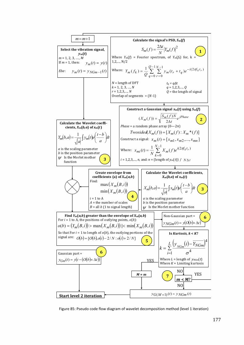
177
Calculate the Wavelet coefficients, Xm(b,a) of xm(t)
a is the scaling parameter b is the position parameter
Is the Morlet mother function
3 ( ) ( ) dta
bttx
aabX mm
−= ∫ ψ
1,
ψ
Create envelope from coefficients (a) of Xm(a,b)
Find:
i = 1 to A A = the number of scales
B = all b (1 to signal length)
4
( )( )( )( )iBX
iBX
m
m
,min
,max
Select the vibration signal, ym(t)
m = 1, 2, 3, ...., M
If m = 1, then:
Else : )()( 1 tyty NGmm −=
)()( tytym =
Calculate the signal’s PSD, Sm(f)
Where Ym(f) = Fourier spectrum, of Ym(fk) for, k =
1,2,..., N/2
Where:
N = length of DFT
k = 1, 2, 3, ..., N r = 1,2,3,..., N
Overlap of segments = (N-1)
1 2)(
2)( fY
N
tfS mm
∆=
∑ ∑−
=
−
=
−+=1
0
1
0
)2()(
1)(
Q
q
N
r
tfiqrmkm
rkettyQ
fYπ
tq = qΔt q = 1,2,3,..., Q
Q = the length of signal
Construct a Gaussian signal xm(t) using Sm(f)
Phase = a random phase array (0—2π)
Construct a signal:
Where:
i = 1,2,3,..., n, and: n = (length of ym(t)) /
2 jPhasem
m et
NfSfX
∆=
2
)())((
],...,,[)( 21 mnmmm xxxtx =
∑−
==
1
0
)2()(
1)(
N
k
tfimmi
rkefXN
txπ
)](*:)([))(( fXfXfXTwosided mmm =
tN ∆
Calculate the Wavelet coeffi-
cients, Xm(b,a) of xm(t)
a is the scaling parameter b is the position parameter
Is the Morlet mother
function 3
( ) ( ) dta
btty
aabY mm
−= ∫ ψ
1,
ψ
Find Ym(a,b) greater than the envelope of Xm(a,b)
For i = 1 to A, the positions of outlying points, o(b):
So that For i = 1 to l ength of o(b), the outlying portions of the
signal are:
5
( )( ) ( )( ) ( )( )iBXiBXiBYbo mmm ,min||,max,)( <>=
( ) ( ) ( ) ( ) ]/2:/2,[ NioNiobObO +−=
YES
m < M?
Non-Gaussian part =
( )( )tbOytNGmy ∆×=)(
1+=mm
)()()1( tNGmytMGy =+
Is Kurtosis, k < K?
Where L = length of yNGm(t) Where K = Limiting kurtosis
( )( )44
1 σ
NGmL
i
Yiyk NGm
−∑==
YES NO
Gaussian part =
( )( )( )tbOtytyGm ∆×−=)(
Start level 2 iteration
M = m
NO
6
6
7
Figure 85: Pseudo code flow diagram of wavelet decomposition method (level 1 iteration)

178
Is Kurtosis, k < K?
Where L = length of ym(t)
Where K = Limiting kurtosis
( )( )44
1 σ
NGmL
i
Yiyk NGm
−∑==
Start level 2 iteration
NO
YES
Calculate the signal’s PSD, Sm(f)
Where Ym(f) = Fourier spectrum, of Ym(fk) for, k = 1,2,..., N/2
Where:
N = length of DFT k = 1, 2, 3, ..., N
r = 1,2,3,..., N Overlap of segments = (N -1)
1 2
,, )(2
)( fYN
tfS smsm
∆=
∑ ∑−
=
−
=
−+=1
0
1
0
)2(,, )(
1)(
Q
q
N
r
tfiqrsmksm
rkettyQ
fYπ
tq = qΔt q = 1,2,3,..., Q
Q = the length of signal
Construct a Gaussian signal xm(t) using Sm(f)
Phase = a random phase array (0—2π)
Construct a signal:
Where:
i = 1,2,3,..., n, and: n = (length of ym,s(t)) /
2 jPhasesm
sm et
NfSfX
∆=
2
)())((
,,
∑−
==
1
0
)2(,, )(
1)(
N
k
tfismsim
rkefXN
txπ
)](*:)([))(( ,,, fXfXfXTwosided smsmsm =
tN ∆
],...,,,[)( ,3,2,1,, snmsmsmsmsm xxxxtx =
s = 1, 2, 3, ...., S If s = 1, then:
Else:
)()(, tyty Gmsm =
)()( 1,, tyty sNGmsm −=
If m = 1, segment = 1
Else
segment = segment
Calculate the Wavelet coefficients, Xm(b,a) of xm(t)
a is the scaling parameter b is the position parameter
Is the Morlet mother function
3
( ) ( ) dta
bttx
aabX smsm
−= ∫ ψ,,
1,
ψ
Create envelope from coefficients (a) of Xm(a,b)
Find:
i = 1 to A A = the number of scales
B = all b (1 to signal length)
4
( )( )( )( )iBX
iBX
sm
sm
,min
,max
,
,
Calculate the Wavelet coeffi-cients, Xm(b,a) of xm(t)
a is the scaling parameter b is the position parameter
Is the Morlet mother function
3
( ) ( ) dta
btty
aabY smsm
−= ∫ ψ,,
1,
ψ
Find Ym(a,b) greater than the envelope of Xm(a,b)
For i = 1 to A, the positions of outlying points, o(b):
So that For i = 1 to l ength of o(b), the outlying portions of the
signal are:
5 ( )( ) ( )( ) ( )( )iBXiBXiBYbo smsmsm ,min||,max,)( ,,, <>=
( ) ( ) ( ) ( ) ]/2:/2,[ NioNiobObO +−=
YES
s < S?
Non-Gaussian part =
( )( )tbOyty sNGm ∆×=)(,
)()( ,)1,( tyty sNGmsmG =+
YES NO
Gaussian part =
( )( )( )tbOtyty sGm ∆×−=)(,
PROCESS DATA SEGMENTS
S = s
NO
6
6
7
Is Kurtosis, k < K?
Where L = length of ym(t)
Where K = Limiting kurtosis
( )( )44
,
1
,
σ
sNGmL
i
Yiyk
sNGm−
∑==
Ym(t) = Ym,1(t)
1+= ss
8
Figure 86: Pseudo code flow diagram of wavelet decomposition method (level 2 iteration)

179
Store: PSDs, RMS levels, durations
for each segment:
),(
),(
),( )(
sm
sm
sm
T
RMS
fS
9
Apply PSDs of segments
in random order creati ng
time domain signals of
segment duration.
As in Step 2.
So that a simulation
signal , xSIM(t), is created.
10
n
iy
RMS
n
ism
sm
∑== 1
2),(
),(
)(
PROCESS DATA SEGMENTS
Figure 87: Create simulation signal, from data segments, for use on vibration table
8.2 Illustrated Use of the Wavelet Decomposition Approach
To illustrate the proposed method and its relevance, an example vehicle vibration
from a supermarket home delivery vehicle is used. The data was collected using a
Lansmont Saver 9x30 field data recorder. This was located on the floor of the
vehicle above the kerb side rear tyre, as this is the position that tends to receive
the worst case vibration (Figure 88).
Figure 88: Home delivery vehicle with location of Saver 9x30 unit

180
The vibration from the journey was measured in one minute samples with zero
spacing to allow for continuous data sampling. A four minute portion of the
journey was used to form an example of the analysis process. The time history
vertical vibration signal is shown in Figure 89.
0 20 40 60 80 100 120 140 160 180 200 220 240-2
-1
0
1
2
3
4
Time (seconds)
Acc
eler
atio
n (
g)
Figure 89: Time history vibration signal
8.2.1 Worked Example of the Ten Step Wavelet Decomposition
Method
The nine steps of the wavelet decomposition method are presented respect to the
vibration signal given in Figure 89.
Step 1 - Calculating the PSD: The signal’s PSD, given in Figure 90, illustrates the
average frequency content of the signal.

181
100
101
102
10-6
10-5
10-4
10-3
10-2
Frequency (Hz)
Po
we
r (g
2/
Hz)
PSD (g2/H
z)
Figure 90: PSD calculated for the vibration signal
The RMS acceleration distribution of one second samples of the signal is given in
Figure 91, the variation in the RMS acceleration distribution indicates that the
signal is non-stationary.
0 0.1 0.2 0.3 0.4 0.5 0.6 0.7 0.8 0.90.90
5
10
15
20
25
30
RMS (g)
Dis
trib
uti
on
(%
)
Figure 91: RMS acceleration distribution
Step 2 - Constructing a Gaussian equivalent signal: By taking the signal’s PSD
(Figure 90) and applying a random phase array, a Gaussian signal with the
equivalent power content of the original signal is constructed (Figure 92).
RMS acceleration (g)

182
0 20 40 60 80 100 120 140 160 180 200 220 240-2
-1
0
1
2
3
4
Time (seconds)
Acc
eler
atio
n (
g)
Figure 92: Simulated Gaussian signal
Step 3 - Perform wavelet analysis on vibration signals: The Morlet mother
function is used to carry out wavelet analysis. A scalogram indicating the variation
in the vibration signal’s wavelet coefficients is given in Figure 93. The wavelet
coefficients for the Gaussian signal are also calculated.
Time (or Space) b
Scal
es a
0.5 1 1.5 2 2.5 3 3.5 4
x 105
1 5 9
13172125293337414549535761
0 2 4 6 8 10
x 10-5
Figure 93: Wavelet analysis of vehicle vibration signal
Step 4 - Create Gaussian envelope: By finding the maximum and minimum
wavelet coefficients for each scale (a) a filter can be created. This filter of the
maximum and minimum Gaussian signal coefficients is shown in Figure 94.

183
1 6 11 16 21 26 31 36 41 46 51 56 61-2
-1.5
-1
-0.5
0
0.5
1
1.5
22
Scale (a)
Wa
ve
let
Co
eff
icie
nt
Va
lue
Figure 94: Limiting Gaussian envelope to identify outliers
Step 5 - Compare vibration signal’s wavelet coefficients with the Gaussian
envelope: The envelope containing the maximum and minimum Gaussian signal
wavelet coefficients are compared with the vibration signal’s wavelet coefficients.
Coefficients that exceed the envelope are identified as points in Figure 95.
0 20 40 60 80 100 120 140 160 180 200 220 24016
1116212631364146515661
Time (Seconds)
Sca
le (
a)
Figure 95: Outliers identified using the Gaussian envelope
Step 6 – Remove non-Gaussian segments from the vibration signal: Segments
of the signal surrounding the position (b) of the outlying coeffient are extracted.
Here a segment length of one second has been used to allow for accurate frequency
content calculations down to 1 Hz. Figure 96 indicates the segments of the
vibration signal extracted to form the non-Gaussian part, with the remaining parts
forming the Gaussian approximation.

184
0 20 40 60 80 100 120 140 160 180 200 220 240-2
-1.5-1
-0.50
0.51
1.52
2.53
3.54
Time (seconds)
Acc
ele
rati
on
(g)
'non-Gaussian'
'Gaussian'
Figure 96: ‘Gaussian’ and ‘non-Gaussian’ segments of the signal
Step 7 - Evaluate the non-Gaussian signal part: The kurtosis of the Gaussian
approximation is 6.5. In this example a limiting value of k = 4 has been set. Because
the kurtosis exceeds this, the iteration process Steps 1-6 are repeated with the non-
Gaussian part being used as the vibration signal.
The process is repeated until all the data fits within a Gaussian approximation or a
limiting number of iterations is reached. For this example, M = 3.
Step 8 - Evaluate the Gaussian approximations: The original vibration signal has
therefore been decomposed into four Gaussian approximations, during the first
level of iteration. The duration, overall RMS acceleration and kurtosis for each part
is given in Table 21.
Table 21: Statistics for each Gaussian approximation produced
during the first level of iteration
ITERATION
NUMBER
DURATION
(Seconds)
RMS
ACCELERATION (g)
KURTOSIS,
k
1 86 0.082 6.5
2 45 0.154 4.6
3 20 0.166 4.2
4 89 0.251 12.5
While the values of kurtosis for segments 2 and 3 are relatively close to that for a
Gaussian distribution (kurtosis of 3), the kurtosis of segments 1 and 4 are not. In

185
particular, segment 4 has a much higher kurtosis of 12.5. The reasoning for this is
that segment 4 (the fourth Gaussian approximation) is actually formed from the
final non-Gaussian part, from the first level of iterations. It therefore contains all of
the shock events from within the original signal and their surrounding vibration,
which did not fit within a Gaussian approximation. If the original signal contains
high level shock events, the wavelet decomposition method will always result in
one final Gaussian approximation that is highly non-Gaussian, this is a limitation of
the method and is discussed further in section 8.4.
The PSD of each part is given in Figure 97. The variation in spectral shape between
the four segments is noticeable, particularly in the shape of the second spectral
peak at around 15 Hz.
100
101
102
10-7
10-6
10-5
10-4
10-3
10-2
Frequency (Hz)
Po
we
r (g
2/H
z)
Segment 1
Segment 2
Segment 3
Segment 4
Figure 97: Average PSD of the ‘Gaussian’ segment for each iteration (level 1)
Because the kurtosis of each Gaussian approximation exceeds the liming value of 4,
each segment is subjected to a second level of iteration to decompose it into
smaller parts with distributions closer to Gaussian.
Steps 1-7 are repeated for a specified number of iterations (S = 2) or, until the non-
Gaussian part is approximately Gaussian (k < 4).
Frequency (Hz)
PS
D (
g2/
Hz)

186
For this simulation, two iterations are made during the second level of
decomposition because of the reduced data set being used (four minute duration).
Carrying out further iterations would create undesirable small duration data
segments, which would present a problem due to the limitations of laboratory
controllers for simulating vibration for such short durations.
The second level of iteration resulted in eight Gaussian segments. The duration,
RMS acceleration and kurtosis relating to the vibration segments are given in Table
22. As with the first level of iteration, whilst the majority of segments have a
kurtosis relatively close to the Gaussian value of 3, the final segment (8) has a
much higher kurtosis. This is again due to the final segment containing all of the
shock events from within the original signal and is a limitation of the wavelet
decomposition method. This is discussed further in Section 8.4
Table 22: Statistics for each Gaussian part from second level of iteration
PART
NO
1ST LEVEL
ITERATION
(m)
2ND LEVEL
ITERATION
(s)
DURATION
(Seconds)
RMS
ACCELERATION
(g)
KURTOSIS
(k)
1 1 1 41 0.037 5.2
2 2 2 5 0.113 3.7
3 3 1 40 0.108 4.2
4 4 2 5 0.130 4.0
5 1 1 39 0.156 4.6
6 2 2 20 0.166 4.2
7 3 1 9 0.164 5.6
8 4 2 81 0.259 12.2
Step 9 - Convert each segment into PSD and RMS acceleration value: In order to
create a simulation, the PSD for each segment has been calculated.
Step 10 - Create a simulation signal: To create a simulation signal, each
segment’s PSD is applied in a random order and an equivalent signal is created.
The resulting simulation signal is shown in Figure 98. Overall, this is both non-
Gaussian and non-stationary.

187
0 20 40 60 80 100 120 140 160 180 200 220 240-2
-1
0
1
2
3
4
Time (seconds)
Acc
ele
rati
on
(g
)
Figure 98: Wavelet decomposition method - simulation signal
8.3 Evaluation of the Wavelet Decomposition Method
By applying the wavelet decomposition method to a non-Gaussian and non-
Stationary vibration signal, it is possible to decompose the signal and represent it
as a series of stationary Gaussian parts. To assess the appropriateness of the
method, comparisons between the PSD, RMS acceleration distribution and
acceleration distribution, of the original vibration signal (Figure 89) and the
simulation signal (Figure 98) are given in Figure 99, Figure 100 and Figure 101,
respectively.
From these results, it can be deduced that the power distribution of the simulated
signal shows good correlation with the power distribution of the original signal.
The RMS acceleration distribution of the simulated signal correlated well with the
original signal in the range 0 - 0.3g. But above 0.3g it did not recreate the
distribution. By increasing the number of iterations made during the second level
of decomposition, and/or reducing segment size, a more accurate representation
of the RMS acceleration distribution could be gained. By carrying out relatively low
resolution decomposition (i.e. a low number of iterations) there will still be an
aspect of signal averaging and therefore the method will produce a slightly
moderated simulation. Following the second level of iteration this stage the
kurtosis of most segments was approximately 4, but for others (such as segment 8)
Time (seconds)
Acc
ele
rati
on
(g
)

188
the kurtosis was much higher. These segments could therefore benefit from
further analysis. In this example, a limit to the number of segments was imposed so
as to avoid skewing the results of the process by creating too small a segment size
for accurate frequency analysis.
100
101
102
10-6
10-5
10-4
10-3
10-2
Frequency (Hz)
PSD
(g2
/Hz)
Original signal
Simulated signal
Figure 99: Average PSD comparison of original vibration signal and simulation signal
0 0.1 0.2 0.3 0.4 0.5 0.6 0.7 0.8 0.9 10
2
4
6
8
10
12
14
16
18
20
22
24
26
28
30
RMS (g)
Dis
trib
uti
on
(%
)
Orignal Signal
Wavelet Approximation
Figure 100: RMS acceleration level distribution comparison of original and simulation signal
RMS acceleration (g)

189
-1 -0.5 0 0.5 10
5
10
15
20
25
Acceleration (g)
Dis
trib
uti
on
(%
)
Wavelet Approximation
Original Signal
Figure 101: Acceleration level distribution comparison of original and simulation signal
8.4 Benefits and Limitations of the Wavelet Decomposition
Method
Being usable on existing controllers is a key requirement of any new simulation
method. The wavelet decomposition method produces a simulation that recreates
a vehicle vibration’s non-stationary and non-Gaussian nature, in a manner that can
be applied to existing controllers. The wavelet decomposition method represents a
signal as a series of PSDs of varying duration. These PSDs can be applied at random
on any existing simulation table controller, to create a series of random vibration
segments, which together build a non-stationary and non-Gaussian representation
of the original signal.
The series of Gaussian approximations, resulting from a signal’s decomposition,
are assumed to be stationary with a Gaussian distribution. Segment 4, from the
first level of decomposition shown in Table 21, has a kurtosis of 12.5, this means
that it has a non-Gaussian distribution. Additionally, the short duration, high
acceleration shock events interspersing the vibration, make the segment non-
stationary. Further iteration of this segment may result in several parts that have a
distribution closer to Gaussian, but due to the nature of vehicle vibration the final

190
Gaussian approximation, which contains the discrete high level shock events, will
always exist.
Whilst the nature of the vibration limits the accuracy of the Gaussian
approximations, the segment size used in the decomposition of the signal also has
an effect. To enable accurate frequency analysis of each Gaussian approximation, a
minimum segment size used for decomposition needs to be enforced. For the
purpose of analyzing vehicle vibration it is suggested that when decomposing a
signal, the minimum size of any segment removed from the signal is one second.
This then allows for frequency analysis from 1 Hz. This limit on the minimum
segment size means that when analysing signals high amplitude shock events of
sometimes millisecond duration, will be incorporated within a segment with much
lower amplitude vibration. These segments will have highly non-Gaussian
distributions, thereby strengthening the limitation that the wavelet decomposition
method will always produce one Gaussian approximation that is highly non-
Gaussian.
Although the aforementioned limitation exists, the wavelet decomposition method
offers much improvement on the current established method, by allowing the non-
stationary and non-Gaussian nature of actual vehicle vibration to be simulated.
Furthermore, due to the complexity of the wavelet decomposition method, a large
memory capacity is required. This is particularly true for long duration
distribution journeys where it may be more appropriate to divide a journey into
parts for analysis. Limitations in computing capacity can limit the frequency
resolution of the wavelet analysis, which is defined by the number of scales used.
The fewer scales used, the low is the frequency resolution and therefore the less
definition in the signal decomposition.
Although there are limitations to this method, the results of this study have shown
that the wavelet decomposition method can be used to decompose a non-Gaussian,
non-stationary vehicle vibration into stationary parts each with an approximately
Gaussian distribution.

191
Furthermore, the use of PSDs in creating the simulation means that it is easily
adaptable for test acceleration using the existing approach.
8.5 Evaluating the Wavelet Decomposition Method using
Damage Correlation
Correlation studies are an important part of validating a simulation method, as
they allow a method to be validated using real measured damage. Therefore, to
evaluate the ability of the wavelet decomposition method for simulating vehicle
vibration, a damage correlation study using the damage mechanism of scuffing has
been carried out using the same time history presented in Figure 43, section 5. The
damage produced using the wavelet decomposition method was then compared
with the damage produced by other simulation approaches.
In order to further validate the method, an additional vibration time history of a
more severe distribution journey is also evaluated. The damage produced using
both vibration profiles shows good correlation between the wavelet
decomposition method and the time history replication.
8.5.1 Methodology
Testing was carried out using the vehicle vibration signal defined in section 5. The
vibration signal time history, RMS acceleration distribution and PSD are illustrated
in Figure 43, Figure 45 and Figure 46, respectively.
Wavelet decomposition has been carried out in Matlab using the code provided in
Appendix V. During the first level of decomposition the time history signal was
decomposed into 12 parts, which were further decomposed in to a maximum of 3
parts. In total, the signal was decomposed into 21 parts. The RMS acceleration,
kurtosis and duration of each part is presented in Table 23.

192
Table 23: RMS acceleration, kurtosis and duration of each signal segment
SEGMENT KURTOSIS,
K
RMS
ACCELERATION (g)
DURATION
(Seconds)
1 4.9 0.150 495
2 4.4 0.235 59
3 3.2 0.249 2
4 3.2 0.260 3
5 3.7 0.270 13
6 3.3 0.303 4
7 3.1 0.255 2
8 13.5 0.335 21
9 5.0 0.130 525
10 4.2 0.221 11
11 4.8 0.262 4
12 4.6 0.223 4
13 3.3 0.218 12
14 4.1 0.279 43
15 4.9 0.148 489
16 4.4 0.237 60
17 3.3 0.250 8
18 3.6 0.268 16
19 3.3 0.303 4
20 3.6 0.235 3
21 13.2 0.338 21
By randomly applying each the PSD of each segment, for the appropriate duration,
the simulated signal shown in Figure 102 (b) was produced.

193
0 200 400 600 800 1000 1200 1400 1600 1800-2
-1
0
1
2
3
4
Time (seconds)
Acc
eler
atio
n (
g)
0 200 400 600 800 1000 1200 1400 1600 1800-2
-1
0
1
2
3
4
Time (seconds)
Acc
eler
atio
n (
g)
Simulated signal
Original signal
Figure 102: (a) Original vibration signal (b) Simulation signal using wavelet decomposition
The scuff rig defined in section 5.1 was used to evaluate the accuracy of the
Wavelet decomposition method and to allow comparison with other simulation
approaches.
Testing was carried out twice using two samples of smooth printed clay-coated
board with sun ‘blue 10’ flexo graphic ink. The first sample, sample A, was from the
batch produced during the testing carried out in section 5.5, therefore the scuff
damage produced during test A can be compared with the results in section 5. The
second sample, sample B, was produced using a slightly different consistency of
sun ‘blue 10’ ink and cannot therefore be compared with previous results.
8.5.2 Evaluation of the Simulated Signal
Although the simulated signal does not fully resemble the original signal, it does
replicate some of the variation in acceleration levels which are characteristic of
vehicle vibration. A comparison of the overall kurtosis and RMS acceleration of the
original signal and the simulated signal is given in Table 24. The error between the
overall RMS acceleration is 0.002g, which is relatively small and would therefore
(a)
(b)

194
suggest good correlation between the overall amplitude of the two signals. The
simulated signal has a kurtosis of 5.6, which signifies a non-Gaussian distribution.
The kurtosis of the original signal is 7.4. The variation between the two is due to
averaging in the wavelet decomposition method.
Table 24: Kurtosis and RMS acceleration of the
original and the simulated signal
SIGNAL KURTOSIS,
k
RMS
ACCELERATION (g)
Original 7.4 0.158
Simulated 5.6 0.156
The PSD of the original signal and the simulated signal is given in Figure 103.
100
101
102
10-10
10-8
10-6
10-4
10-2
Frequency (Hz)
PS
D (
g2/H
z)
Original signal
Simulated signal
Figure 103: PSDs for original time history signal and simulated signal using wavelet decomposition
The shape of the simulated signal’s PSD correlates with the original vibration
signal’s PSD, with only a small amount of error between the two, this error is
presented in Figure 104. Only the frequency range 1 - 30 Hz is shown as the error
in frequencies above this is comparatively low. The error in the PSD is greatest in
the low frequency range (1 – 10 Hz), this is because the power within the low
frequency range is much greater than that at higher frequencies. Therefore as a

195
percentage, the error within the low frequency range is much smaller than that at
higher frequencies.
0 5 10 15 20 25 30-2
-1
0
1
2
3
4x 10
-3
Frequency (Hz)
Err
or
in P
SD (
g2/H
z)
Figure 104: Error in simulated signal’s PSD by comparison to original vibration signal’s PSD
The RMS acceleration distribution for one second samples of both the original
signal and the simulated signal are given in Figure 105.
0 0.1 0.2 0.3 0.4 0.50
5
10
15
20
25
30
35
40
RMS (g)
Occ
ure
nce
(%
)
Original
Simulated
Figure 105: RMS acceleration distribution for original time history signal and simulated signal using
wavelet decomposition
Frequency (Hz)
Err
or
in P
SD
(g
2/
Hz)
RMS acceleration (g)
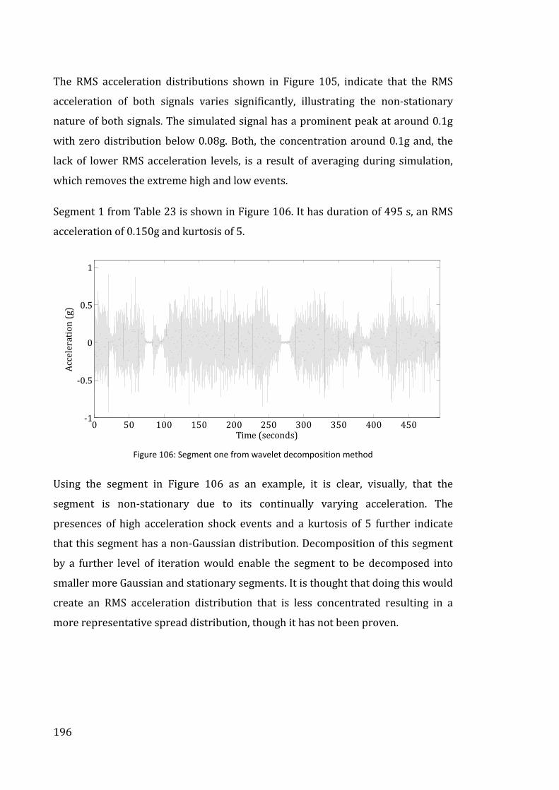
196
The RMS acceleration distributions shown in Figure 105, indicate that the RMS
acceleration of both signals varies significantly, illustrating the non-stationary
nature of both signals. The simulated signal has a prominent peak at around 0.1g
with zero distribution below 0.08g. Both, the concentration around 0.1g and, the
lack of lower RMS acceleration levels, is a result of averaging during simulation,
which removes the extreme high and low events.
Segment 1 from Table 23 is shown in Figure 106. It has duration of 495 s, an RMS
acceleration of 0.150g and kurtosis of 5.
0 50 100 150 200 250 300 350 400 450-1
-0.5
0
0.5
1
Time (seconds)
Acc
eler
atio
n (
g)
Figure 106: Segment one from wavelet decomposition method
Using the segment in Figure 106 as an example, it is clear, visually, that the
segment is non-stationary due to its continually varying acceleration. The
presences of high acceleration shock events and a kurtosis of 5 further indicate
that this segment has a non-Gaussian distribution. Decomposition of this segment
by a further level of iteration would enable the segment to be decomposed into
smaller more Gaussian and stationary segments. It is thought that doing this would
create an RMS acceleration distribution that is less concentrated resulting in a
more representative spread distribution, though it has not been proven.

197
8.5.3 Results
The percentage of scuff damage produced from a time replication simulation and
wavelet decomposition method is shown for Test A in Table 25, and, for Test B in
Table 26.
Table 25: Test A percentage scuff damage using time replication and wavelet decomposition
TEST
(A)
SIMULATION
APPROACH
PERCENTAGE
SCUFFING
INCLUSION OF
5% ERROR
VARIATION
FROM TIME
REPLICATION MAX MIN
1 Time Replication 0.60% 0.63% 0.57% -
2 Wavelet Decomposition
Method 0.56% 0.59% 0.53% -7%
Table 26: Test B percentage scuff damage using time replication and wavelet decomposition
TEST
(B)
SIMULATION
APPROACH
PERCENTAGE
SCUFFING
INCLUSION OF
5% ERROR
VARIATION
FROM TIME
REPLICATION MAX MIN
1 Time Replication 0.71% 0.75% 0.67% -
2 Wavelet Decomposition
Method 0.80% 0.84% 0.76% 13%
8.5.4 Comparison of Results Using other Simulation Methods
The resulting level of scuff damage, using sample A, is presented in Figure 107 with
the results from the previous correlation study.
The results show good correlation between the first and second time replication
simulation with, 0.59% and 0.60% scuff damage, respectively. The level of scuff
damage produced using the wavelet decomposition method correlates well with
both time replication tests with the error in the level of scuff damage being 5% and
7%, respectively.
When compared with the other simulation approaches, the wavelet decomposition
method shows the highest correlation with the modulated RMS approach.

198
0.60.56
0.590.56
0.64
0.81
0.27
0.18
0.1
0.00
0.10
0.20
0.30
0.40
0.50
0.60
0.70
0.80
0.90
Per
cen
tage
Scu
ffin
g (%
)
Results from Test A
Results fromprevious study
Figure 107: Percentage level of scuff damage for different simulation approaches
Overall, the samples used in Test B produced a higher level of scuff damage in both
tests. This was due to the change in consistency of the ink used. When compared to
Test A, Test B produced a slight over test of 13%.
In both tests, the wavelet decomposition method was shown to correlate well with
vertical vibration time replication, with Test A producing a slight under test of 7%,
and Test B producing a slight over test of 13%.
The level of damage produced from the wavelet decomposition method in Test A
correlated well with the RMS modulation approach. However, the results in Test B
correlated better with the accelerated PSD where the time was compressed by 5
and k = 2, producing over tests of 13% and 14%, respectively.
This variation in results could be due to test errors as it was shown by Shires et al
(2010) that the scuff rig had a confidence limit of 95% with an error margin of 5%.
This error is typically produced by the method of measuring the scuffing. This
variation in the over and under test may therefore be due to test error. To evaluate

199
the method further, the Wavelet decomposition method has been used to simulate
an additional journey. The results from this testing are now presented.
8.5.5 Simulating an Alternative Journey Using Wavelet
Decomposition Method
To further validate the use of the wavelet decomposition method, additional
analysis and experimentation has been carried out on an additional, more severe
journey. The time history vehicle vibration is given in Figure 108. Using the
wavelet decomposition method, a simulation signal was produced.
0 200 400 600 800 1000 1200 1400 1600 1800-3
-2
-1
0
1
2
3
Time (seconds)
Acc
eler
atio
n (
g)
Figure 108: Time history vehicle vibration signal
8.5.6 Comparison of Results
The percentage scuff damage produced using the wavelet decomposition method and time replication
of the time history, is shown in
Table 27. In Test C the wavelet decomposition method correlates well with the
time replication with only 8% error in the level of scuff damage. Similar to Test B,
the wavelet decomposition method produced an over test in comparison with the
time replication simulation.

200
Table 27: Percentage scuff damage produced for the simulation methods
TEST
(C)
SIMULATION
APPROACH
PERCENTAGE
SCUFFING
INCLUSION OF
5% ERROR
VARIATION
FROM TIME
REPLICATION MAX MIN
1 Time Replication 1.15% 1.21% 1.09% -
2 Wavelet Decomposition
Method 1.24% 1.30% 1.18% 8%
8.6 Concluding Remarks
Throughout this chapter the wavelet decomposition method has been explained in
detail and the process of producing a simulation has been described. It has been
shown, through theoretical evaluation, that by simulating the original signal as a
series of Gaussian approximations of varying RMS acceleration and spectral
content, the method manages to recreate part of the signal’s non-stationarity and
non-Gaussian distribution.
The wavelet decomposition method has been proven for both example time
histories to correlate well with time replication simulation. In Test A the
percentage error in damage correlated well with RMS modulation, in Tests B and C
the percentage error correlated better with the single level PSD where the time
was compressed by 5 and k = 2.
In two out of the three simulations the wavelet decomposition method produced a
slight over test in comparison to the single axis time history replication.
When considering vehicle vibration, which is known to be highly non-stationary
and non-Gaussian, being able to distinguish points within the signal which make it
so, is beneficial within the analysis process. By making use of time-frequency
analysis, the wavelet decomposition method is able to decompose a non-Gaussian
and non-stationary signal into its approximately Gaussian and stationary parts.
Shown here and within sections 8.2 and 8.3 is that the simulation produced
through the random synthesis of these parts is, overall, non-stationary in both the

201
time (evident in the varying RMS acceleration distribution) and frequency domain
(evident in the changing shape of the PSD) and, has a non-Gaussian distribution
(evident in the measure of kurtosis). This allows a signal's characteristics in the
time and frequency domain to be considered together, which is in contrast to the
established method.
The example given in this study has shown how the wavelet decomposition
method is used to create a simulation representative of actual vehicle vibration.
However, the RMS acceleration distribution of the simulated signal deviated from
that of the original signal. If the Gaussian approximations, produced during the
second level of iteration, were decomposed further, it is possible that a simulated
signal with an RMS acceleration distribution, matching better that of the original
signal, could be formed, though this has not been proven.
Through theoretical work, the wavelet decomposition method’s ability to replicate
the statistical content of vehicle vibration has been examined and proven. In order
to evaluate the method’s appropriateness in recreating the extent of product
damage during distribution, a correlation study measuring damage has been
carried out and is now discussed.

202
9 APPROXIMATING VEHICLE VIBRATION
AND ROAD ROUGHNESS USING
COMPUTATIONAL VEHICLE MODELS
The use of a vehicle model to approximate a vehicle’s vibration response to that of
a given road profile in order to create a representative test for distribution
packaging was first proposed by Rouillard (2008). In this chapter a simplified
quarter vehicle model and a known road profile were used to calculate the
vehicle’s response. Doing so allows for variations in: the vehicle’s payload;
suspension; tyre stiffness; and, speed; to be accounted for when producing a
simulation test.
Over the last two decades various vehicle models have been proposed which vary
in detail and complexity, including quarter car, half car and full vehicle models
(Rajamani, 2012; Pacejka, 2006). Vehicle models are constructed from an array of
mass-spring-dampers placed in series and in parallel which model the vehicle’s
suspension and tyre systems. The complexity of these vehicle models varies
depending on the accuracy and detail of the model and information required from
it. Specialised computer programs exist for the simulation of vehicles, including:
Adams©, which is a multi-body dynamic simulation program enabling the user to
construct complex vehicle models for vehicle simulation and optimisation;
Vehiclesim©, which is a programme that specialises in vehicle simulation; and,
Mathworks Simulink©, which contains toolboxes from which the user can
construct a vehicle model.
For the purpose of this work, the vehicle model is only required to simulate the
vehicle movement and not to optimise the model, additionally the model must be
compatible with Matlab programming. Therefore Simulink has been used to create
vehicle models. Both the full vehicle and quarter vehicle models are now discussed.

203
9.1 Review of Vehicle Models
For the purpose of this research, both the full car model and quarter car model
have been considered. The benefits and limitations of each are discussed, in order
to provide reasoning behind the use of either for the purpose of generating a
simulation regime for packaging distribution. An appropriate vehicle model has
then been developed for the purpose of creating an improved simulation regime
and also for the purpose of generating road roughness profiles from vehicle
vibration data.
9.1.1 Full Vehicle Model
A full vehicle model is the most complete, allowing the user to approximate the full
motion of the vehicle along all of its linear and rotational axes. The complexity of
this model is dependent on the detail of the vehicle. For instance, in contrast to a
car, which has a single body, a semi-trailer (where a coupling system connects the
driver’s cabin and trailers) has more degrees of freedom and constraints making it
much more complex. This can be seen in the vehicle models shown in Cheng and
Cebon (2008) and Miege and Cebon (2005).
For the purpose of this study, where the input to the vehicle model is the vertical
displacement of the road profile, the lateral, longitudinal and yaw components of
the vehicle cannot be considered. Therefore by using a full vehicle model to
simulate the vehicle’s vibration response, vibration in only the vertical, pitch and
roll axes can be calculated to evaluate an MDOF response of the vehicle. In order to
do this accurately, the road roughness must be provided for each point of vehicle
contact with the road and must be in phase. Incorrect recording of the road
profiles or timing of their application can lead to great errors in the calculation of
the vehicle’s pitch and roll.
As only the vertical vibration of the vehicle is considered in the established method
and the wavelet decomposition method, only the vertical component of the vehicle
model used is required.

204
For this purpose, the main benefit of the full vehicle model is that it allows the
vibration response across the vehicle body to be calculated, thus enabling the
consideration of load position and distribution on the vehicle floor. This in turn
would allow for a vibration tests to be constructed suiting the position of the load
within the vehicle.
The variability in parameters and movement in load and position is hard to predict
and therefore, by using the full vehicle model, uncertainties in the vibration
response can exist.
9.2 Quarter Vehicle Model
Rather than consider each wheel and suspension connection separately, the
vehicle is represented as two mass-spring-damper systems with the average
parameter values for the unsprung mass and suspension and tyre system, and, a
quarter of the vehicle mass. The simplicity of the model means that the varied
response across the vehicle cannot be calculated, only a vehicle average.
The quarter vehicle model is shown in Figure 109. It comprises of two mass-
spring-damper systems in parallel, these correspond to the sprung mass
(suspended vehicle), MV, and unsprung mass (wheel system), MT. Both of the
masses are constrained to move only vertically, with displacements x2, and x1,
respectively. The vertical input to the tyre from the road surface is x0. The
suspension stiffness and damping parameters are denoted by KS and CS,
respectively, and the tyre stiffness and damping is denoted by KT and CT,
respectively. By generating the equations of motion for the quarter vehicle model it
is possible to estimate the vehicle’s response to a given road input.

205
Mv
Mt
CS KS
KT CT
x2(t)
x1(t)
x0(t)
Figure 109: Quarter vehicle model
For the quarter vehicle model given in Figure 109 the equations of motion are
derived as:
1121
.
2
.
2
..
)()( FgMxxKxxCxM VSSV ==−+−+ (36)
2010
.
1
.
212
.
1
.
1
..
)()()()( FgMxxKxxCxxKxxCxM TTTSST ==−+−+−+−+ (37)
Incorporating a quarter vehicle model within a new test regime removes the need
for in situ vibration data acquisition and therefore significantly reduces data
collection times.
9.3 Simulink Quarter Vehicle Model
A quarter vehicle model has been constructed using a Simulink block diagram. The
model and its subsystems are shown in Figure 110, Figure 111 and Figure 112. The
input to the model is a vector of the road’s vertical displacement at each sample
time (dt). The output is then the vehicle’s vertical acceleration of the sprung mass
(ddx2). Tyre damping (CT) has not been included in the vehicle models.

206
Figure 110: Simulink quarter vehicle model
Figure 111: Simulink quarter vehicle model subsystem 1 from Figure 110

207
Figure 112: Simulink quarter vehicle model subsystem 2 from Figure 110
9.4 Using the Inverse Quarter Car Model to Approximate
Road Profiles
In addition to approximating the vehicle response, the inverse of the vehicle model
can be used to approximate a road profile from vehicle vibration. This can be done
by inverting the vehicle’s equations of motion making the relevant parameters the
subject:
1
.122
.
2
..
xC
gMxKxKxCxM
S
VSSSV =−−++
(38)
0
0
.
11
.
212
.
1
.
1
..
)()(x
K
gMxCxKxCxxKxxCxM
T
TTTTSST =−−++−+−+
(39)

208
By using the inverse model, a vehicle vibration profile from a specific distribution
route can be used to approximate the vibration profile of any other vehicle
travelling along that distribution route. This allows for a change in distribution
vehicle and/or payload to be accounted for without the need for additional in-situ
data acquisition.
A Simulink model which solves Equations 38 and 39 has been created, to allow the
calculation of an approximate road profile. The structure of the model and its
subsystems is given in Figure 113, Figure 114 and Figure 115, respectively.
Figure 113: Simulink Inverse vehicle model
Figure 114: Simulink inverse quarter vehicle subsystem 1

209
Figure 115: Simulink inverse quarter vehicle subsystem 2
When using the model the initial conditions for each of the parameters are set as
zero, so that when time, t = 0:
( )
02
22
2 ===dt
dxd
dt
dxx
( )0
2
11
1 ===dt
dxd
dt
dxx
00
0 ==dt
dxx
These assumptions lead to errors in the resulting road profile approximation. This
error dissipates with time. An example of the error induced by calculating a road
profile from a given vehicle vibration (Figure 116) using the inverse vehicle model
the approximate road profile is calculated (Figure 117), the quarter vehicle model
is then used to calculate the approximate vehicle vibration (Figure 118). The error
arising between the original vehicle vibration and the approximated vibration
calculated using the vehicle model, is shown in Figure 119.

210
0 10 20 30 40 50 60 70 80 90 100-1.25
-1
-0.75
-0.5
-0.25
0
0.25
0.5
0.75
1
1.25
Time (seconds)
Acc
eler
atio
n (
g)
Figure 116: Example vehicle vibration
0 10 20 30 40 50 60 70 80 90 100-0.075
-0.05
-0.025
0
0.025
0.05
0.075
Time (seconds)
Dis
pla
cem
ent
(m)
Figure 117: Approximate road profile calculated using the inverse quarter vehicle model
0 10 20 30 40 50 60 70 80 90 100-1.25
-1
-0.75
-0.5
-0.25
0
0.25
0.5
0.75
1
1.25
Time (seconds)
Acc
eler
atio
n (
g)
Figure 118: Approximate vehicle vibration calculated using the quarter vehicle model
In Figure 119 a large initial error is visible, this is caused by the approximation of
the initial conditions leading to a significant over approximation causing an over
shoot in the approximated vehicle’s response, though this error dissipates, after
which the error is insignificantly low.

211
10-3
10-2
10-1
100
101
102
-8
-7
-6
-5
-4
-3
-2
-1
0
1
2
Time (seconds)
Acc
ele
rati
on
(g)
Figure 119: Amplitude of error in the calculated vehicle vibration for time history vibration in
The PSD for both the original vibration and that simulated by the quarter vehicle
model, are given in Figure 120. The simulated vibration’s PSD correlates well with
the original signal’s PSD.
1 10 100 20010
-6
10-5
10-4
10-3
Frequency (Hz)
PSD
(g2
/Hz)
SimulatedVibration
OriginalVibration
Figure 120: PSD of original vehicle vibration and vehicle vibration simulated through vehicle model
The error between the original and the simulated signals’ PSDs is given Figure 121.
The error in the low frequency range (1 -10 Hz) is extremely low. Above 30 Hz the
error is significantly higher, with the highest error, of approximately 35%, at
approximately 74 Hz.
Frequency (Hz)
PS
D (
g2/
Hz)
Time (seconds)
Err
or
in a
cce
lera
tio
n (
g)

212
1 10 100 200-10
0
10
20
30
40
Frequency (Hz)
Per
cen
tage
Err
or
(%)
PercentageError
Figure 121: Percentage error between original signal’s PSD and simulated signal’s PSD
The simulated signal showed good correlation with the original signal. The model
is therefore suitable for use in the journey database. Though consideration of the
initial error should be given and this part of the signal removed before further
analysis.
9.5 Quarter Vehicle Model Benefits and Limitations
Although basic, the quarter vehicle model has a number of benefits. Firstly, unlike
the full vehicle model, where several road profile inputs are required, the quarter
vehicle model only requires one. This not only simplifies the process of road profile
data collection but also reduces the computational power required to calculate the
vehicle motion. Secondly, by only having one output, the memory requirement is
significantly reduced compared with that of the full vehicle model. Thirdly, fewer
vehicle parameters are required and, by using the average of the vehicle
parameters, the significance of possible errors in the calculation of individual
vehicle parameters is reduced.
Whilst there are benefits to using a quarter vehicle model, there are also several
limitations that must be considered. The simplicity of the quarter vehicle model
requires the following assumptions to be made:
Frequency (Hz)
Pe
rce
nta
ge
err
or
(%)

213
• Vehicle parameters are deterministic - In reality vehicle parameters can vary
due to: manufacture tolerances; vehicle age; vehicle condition; the distribution
payload; and, the varied and complex interaction of the vehicle with the road
surface. For instance, spring stiffness and damping can differ from the
manufacturer’s value as a result of wear or production tolerances. Additionally,
it is now common for suspension characteristics on vehicles to be designed
specifically for the product they are carrying, resulting in parameters varying
between vehicles.
In the quarter vehicle model, the tyre’s contact with the road surface is
modelled as a point which is in continual contact with the road surface. In
reality the way in which the tyres interact with the road is much more complex.
The constant change in contact area and surface pressure, along with
uncertainties in the static pressure and extend of the wear of tyres, can lead to
stochastic variations in the tyre stiffness that are difficult, if not impossible, to
predict.
Vehicle mass can also vary significantly due to loading and unloading of
products. Additionally, the placement of products in the vehicle for distribution
can lead to variations in vehicle response across the vehicle floor. By using a
quarter vehicle model these variations are either difficult or impossible to
consider.
• The vehicle is symmetrical – Because the quarter vehicle model uses parameter
averages, a uniform load is assumed throughout the vehicle. It is rarely the case
that the vehicle’s centre of gravity will fall directly in the centre of the vehicle
and, the suspension system have the same characteristics left to right and front
to back. Therefore, in reality, the vehicle’s response varies across the vehicle
floor, with the vibration at the rear on the kerb side of the vehicle typically
being the most severe.
• Limited to low frequency range estimation - The quarter vehicle model allows
the calculation of the first and second natural frequencies, arising from the
suspension and wheel system, respectively. The third natural frequency, caused

214
by the structural floor/body of the vehicle, cannot be simulated through a
quarter vehicle model. In order to evaluate this third natural frequency a more
complex model would be required, for which further vehicle parameters
pertaining to the vehicle’s construction would be required. Typically, this
frequency falls within the range 50 – 60 Hz, with a much smaller modal
participation factor than the first two frequencies. It is therefore considered to
have little effect on product damage. The repercussions of this are evident when
a vehicle’s vibration response during a specific distribution journey is used to
approximate another vehicle’s response on that same journey. The low
frequency content of the approximated vehicle response will reflect that of the
simulated vehicle, whilst the high frequency content will not be considered and
therefore will reflect that of the original vehicle. The significance of this depends
on the frequency response of the packaged product being evaluated.
9.6 Sensitivity Analysis of the Quarter Vehicle Model
In order to be able to simulate a vehicle’s vibration response to different road
inputs, the vehicle’s parameters are required. As stated earlier, the assumption
that the parameters are deterministic is not correct. Therefore, it is likely that
errors will arise in the simulated vehicle response due to the incorrect selection of
vehicle parameters. In some cases the use of incorrect parameters has little or no
effect on the vehicle response, but, in other cases these errors can be large and may
significantly alter the simulated response. It is therefore necessary to assess the
effect that errors in parameters have on the estimated response. For the purpose
of this study the Ford Luton Box van from a previous study is used as an example
vehicle, with the correct vehicle parameters assumed to be those shown in Table
28.

215
Table 28: Ford Luton box van parameters
PARAMETER VALUE
MV Vehicle Mass 600 kg
MT Unsprung Mass 50 kg
KS Suspension Stiffness 95 kN/m
CS Suspension Damping 250 Ns/m
KT Tyre Stiffness 285 kN/m
CT Tyre Damping 60 Ns/m
Two measures can be used to evaluate the magnitude of the error: the vehicle’s
natural frequencies; and, the vehicle’s transmissibility. The method of calculating
both the natural frequencies and the transmissibility is now detailed.
9.6.1 Calculating a Vehicle’s Natural Frequencies
The vehicle’s first two undamped natural frequencies, relating to the suspension
and wheel systems, can be found from the Eigen values of the equations of motion
(Equations 36 and 37).
Firstly, the free vibration of the system needs to be considered, where F1 = F2 = 0,
and x1 and x2 are assumed to have the same frequency and expressed in the
complex form:
ti
eXtxω
11 )( = (40)
tieXtx ω
22 )( = (41)
Substituting Equations 40 and 41 into Equations 36 and 37 gives:
[ ] 0)( 211
2 =−+− ti
SV eXXKXM ωω
(42)
[ ] 0)( 1222
2 =−++− ti
STT eXXKXKXM ωω (43)
In matrix format, Equations 42 and 43, can be expressed as:
( )( ) 0
2
1
2
2
=
++−−
−+−
X
X
KKMK
KKM
TSTS
SSV
ωω
(44)

216
Rearranging Equation 44 in to the format [K]{X}= ω2[M]{X} gives:
( )( )
=
+−
−
2
12
2
1
X
X
M
M
X
X
KKK
KK
T
V
TSS
SS ω
(45)
By multiplying both sides of Equation 44 by the inverse of the mass matrix, [M]-1
the equation can be put in the form of the characteristic determinant Ι− λA ,
where:
[ ] [ ]KMA
1−=
+−
−
=
TSS
SS
V
T
VTKKK
KK
M
M
MMA
0
01
and, 2ωλ =
From the characteristic determinant the Eigen values and therefore the natural
frequencies (in Rad/s) can be found, where:
21
2 ωω =n or 22ω (46)
Using the parameters in Table 27, the first and second natural frequency for the
Ford Luton box van were found to be 2.4 Hz and 17.5 Hz, respectively.
9.6.2 Vehicle Transmissibility
Transmissibility measures the energy transferred between the input of a system
and its output. Using the Equations 36 and 37, the transmissibility can be
calculated for the vehicle displacement (x2) in relation to the road profile
displacement (x0). Rearranging Equations 36 and 37 and substituting in Equations
40 and 41, gives:
0)()( 12
2 =+−++− XiCKXiCKM SSSSV ωωω
(47)

217
( ) OTTSSTTSS XiCKXiCKKMXiCK ωωωω +=+++−++− 1
2
2 )()(
(48)
Using matrix multiplication, the transmissibility between the displacement of the
vehicle, 2X , and the input 0X , can be found:
[ ]{ }( )
+
=
01
2 0 =XB
XiCKX
X
cb
ba
TT ω (49)
Multiplying each side by the inverse of matrix B gives:
( )
+
−
−
−=
02
1
2 01
XiCKab
bc
bacX
X
TT ω
(50)
( )
+
++−+
++++−
+−+++−++−=
02
2
2221
2
0
)()(
)()(...
)())((
1
XiCKiCKMiCK
iCKiCKKM
iCKiCKKMiCKMX
X
TTSSVSS
SSSSTT
SSSSTTSSV
ωωωωωωω
ωωωωω
The transmissibility of the vehicle is therefore found from:
( )
2
0
2
bac
iCKb
X
X TT
−
+−=
ω
( ) ( )( ) ( )222222
222
0
2
)())(( TTVSVSTTVS
TSSTTSTS
KMMiCMKMKMK
CCKiCKiCKK
X
X
−++−−−
−++=
ωωωωωω
ωωω (51)
The transmissibility for the Ford Luton box van has been calculated and is given in
Figure 122, where the peaks in the transmissibility can be seen at the first and
second natural frequencies.

218
100
101
102
10-4
10-2
100
102
Frequency (Hz)
Tra
nsm
issi
bil
ity
rat
io (
X2
/X0
)
Figure 122: Ford Luton box van transmissibility (X2/X0)
9.6.3 Suspension Stiffness
The vehicle’s suspension system acts to isolate the vehicle’s structure from
undesirable shock and vibration during transit. This protects the occupants and
load from exposure to high level shock events and excessive vibration, and,
protects the vehicle from excessive fatigue damage, without negatively affecting
the vehicle’s handling and stability.
The suspension stiffness can vary depending on the vehicle mass. Heavier vehicles
require a stiffer suspension and therefore, for example, a semi-trailer will have a
much stiffer suspension than a delivery van. Although a value for the suspension
stiffness may be given by the manufacturer, or, estimated depending on vehicle
type and payload, the stiffness may still vary depending on: the age of the vehicle;
manufacturer’s tolerances; or, vehicle alterations due to its special use. Therefore,
when simulating a vehicle the possible error in suspension stiffness and its effect
on the simulated response needs to be considered.
Figure 123 illustrates how changes in the suspension stiffness affect the vehicle
transmissibility. It can be concluded that the stiffer the suspension, the higher the
transmissibility ratio, particularly around the natural frequency. Increasing the
suspension stiffness also increases the vehicles natural frequencies.

219
10-1
100
101
102
10-4
10-2
100
102
104
Frequency (Hz)
Tra
nsm
issi
bil
ity
rat
io (
X2/X
0)
KS=57 kN/m
KS=114 kN/m
KS=171 kN/m
KS=228 kN/m
KS=285 kN/m
KS=342 kN/m
KS=399 kN/m
KS=456 kN/m
KS=513 kN/m
KS=570 kN/m
Figure 123: Transmissibility for vehicles with varying suspension stiffness, KS
The error in both the first and second natural frequencies with respect to error in
the suspension stiffness is proportional to an order six polynomial, where the
constants are determined by the vehicle’s parameters.
40%
60%
80%
100%
120%
140%
0% 50% 100% 150% 200% 250%
Variation in Suspension Stiffness (Ks) (%)
Err
or
in N
atu
ral
Fre
qu
en
cy (
%)
NF2
NF1
(KS) (%)
Figure 124: Percentage error in natural frequency due to error in suspension stiffness, KS
An example of the change in vibration response for varying suspension stiffness is
shown in Figure 125, where 100% is equivalent to 95 kN/m.

220
10 10.1 10.2 10.3 10.4 10.5-4
-3
-2
-1
0
1
2
3
4
5
Time (Seconds)
Acc
eler
atio
n (
g)
20%
40%
60%
80%
100%
120%
140%
160%
180%
200%
Figure 125: Sample Vibration signal for varying suspension stiffness, KS
Figure 125 indicates that the greater the suspension stiffness, the more severe the
vibration response, due to the suspension system not isolating the input excitation
as effectively. Therefore, it can be concluded that error in the approximation of the
suspension stiffness can lead to relatively significant error in the simulated vehicle
response and hence, careful consideration should be given to the value of the
suspension stiffness used in the vehicle model.
9.6.4 Suspension Dampers
In the suspension system, dampers are used to dissipate any high energy vibration
occurring at and around the suspension’s natural frequency, ensuring that high
energy shock events caused by large displacements in the road surface are not
transferred to the vehicle. The effect of varying the vehicle’s damping on the
transmissibility is illustrated in Figure 126. When the suspension damping is
increased, the transmissibility peak at the suspension’s natural frequency is
reduced.

221
10-1
100
101
102
10-4
10-2
100
102
104
Frequency (Hz)
Tra
nsm
issi
bil
ity
rat
io (
X2/X
0)
CS=50 Ns/m
CS=100 Ns/m
CS=150 Ns/m
CS=200 Ns/m
CS=250 Ns/m
CS=300 Ns/m
CS=350 Ns/m
CS=400 Ns/m
CS=450 Ns/m
CS=500 Ns/m
Figure 126: Transmissibility for varying suspension damping, CS
When modelling a vehicle, as with the suspension stiffness, it is difficult to
calculate the exact suspension damping, CS, value. Therefore it is likely that when
modelling a vehicle errors in the calculation will occur. When considering the
percentage error in the transmissibility at both the first and second natural
frequencies in relation the percentage error in CS, the error relationship is a
polynomial of order six where the values are dependent on the values of the
parameters used.
9.6.5 Tyre Stiffness
Whilst the suspension removes the low frequency high amplitude events, the tyres
remove high frequency low amplitude events, providing a more comfortable ride.
(Garret et al, 2001). The tyres are inflated to a pressure at which they are able to
support the static and dynamic loading of the vehicle. The higher the pressure the
stiffer is the tyre and the more is the energy transmitted to the vehicle and as a
result the more severe is the vibration. The effect of varying vehicle stiffness is
illustrated using the transmissibility plot in Figure 127.

222
10-1
100
101
102
10-4
10-2
100
102
104
Frequency (Hz)
Tra
nsm
issi
bil
ity
rat
io (
X2/X
0)
KT
=57 kN/m
KT
=114 kN/m
KT
=171 kN/m
KT
=228 kN/m
KT
=285 kN/m
KT
=342 kN/m
KT
=399 kN/m
KT
=456 kN/m
KT
=513 kN/m
KT
=570 kN/m
Figure 127: Transmissibility for varying tyre stiffness, KT
9.6.6 Tyre Damping
The level of damping provided by the tyres is relatively low and therefore often
neglected (Wong, 1993). A tyre’s damping rate is also difficult to calculate due to
constant changes in the tyre’s shape, its road contact area and its stiffness. As a
result, most vehicle models omit the tyre damping from calculations. In the quarter
car model used in this study the tyre damping has been accounted for using a low
nominal value with variations in this value having minimal effect on the vehicle
response.
9.6.7 Sprung Mass
Altering a vehicle’s mass affects its first natural frequency. This is typically in the
range 1 – 5 Hz and arises due to resonance in the suspension system. Altering a
vehicle’s mass also affects the amplitude of its peak transmissibility. The variation
in the transmissibility curve for the example vehicle is illustrated in Figure 128.
The frequency of the first natural frequency is inversely proportional to the vehicle
mass, whilst the amplitude of the transmissibility at the natural frequency is

223
proportional. Also evident, is that the vehicle’s mass affects the amplitude of the
transmissibility at the second natural frequency, with it being inversely
proportional to the mass, but it does not affect the frequency.
10-1
100
101
102
10-4
10-3
10-2
10-1
100
101
102
Frequency (Hz)
Tra
nsm
issi
bil
ity
rat
io (
X2/X
0)
MV
=120 kg
MV
=240 kg
MV
=360 kg
MV
=480 kg
MV
=600 kg
MV
=720 kg
MV
=840 kg
MV
=960 kg
MV
=1080 kg
MV
=1200 kg
Figure 128: Transmissibility for varying vehicle Mass, MV (kg)
The relationship between vehicle mass and the first natural frequency is illustrated
in Figure 129. It can be said that the higher the mass (Mv) the less is the effect a
change in the mass will have on the natural frequency.
-80 -60 -40 -20 0 20 40 60 80 100
-40
-20
0
20
40
60
80
100
120
Error in vehicle sprung mass (%)
Ch
ang
e in
na
tura
l fr
eq
uen
cy (
%)
Figure 129: Variation in first natural frequency relative to the variation in vehicle mass, MV

224
To consider how a change in vehicle mass affects a vehicle’s response, the quarter
vehicle model has been used to carry out a comparison of vehicle responses to a
given road input. Figure 130, shows a two second sample from the vibration
response. There is a clear variation in the vehicle’s response, with a lower vehicle
mass corresponding to greater amplitude of the vibration acceleration.
10 10.1 10.2 10.3 10.4 10.5 10.6 10.7 10.8 10.9 11-15
-10
-5
0
5
10
15
20
Time (Seconds)
Acc
eler
atio
n (
g)
20%
40%
60%
80%
100%
120%
140%
160%
180%
200%
Figure 130: Sample vibration signal for varying mass, MV
9.6.8 Payload
Vehicle payload can vary significantly between items of distribution, for example, a
shipment of a high density product such as cola will have a significantly higher
mass than a shipment of a less dense product such as potato crisps. Further
variation in payload may occur during the distribution journey if several
shipments are distributed on one route. The observable variation in vehicle
response for varying vehicle mass, shown in Figure 130, highlights the importance
of ensuring the correct payload is modelled.
The centre of mass of a vehicle will vary depending on the vehicle payload. Whilst
the vehicle is empty, the centre of mass will not be located in the centre of the
vehicle but will be positioned towards the front of the vehicle, where the engine is
located. The effect of this can be accounted for in a full vehicle model and to some
extent in the half vehicle model. However, with the quarter vehicle model, an

225
evenly distributed load is considered and as a result an average vibration is
produced.
9.7 Unsprung Mass
A vehicle can be separated into two defined masses: the sprung mass (MV), which
accounts for all elements of the vehicle supported by the suspension e.g. the
structural body of the vehicle; and, the unsprung mass (MT), which includes all
elements of the suspension system, the wheels and anything else that is connected
to but not supported by these.
Variations in the unsprung mass have a significant effect on the second natural
frequency. This is evident in the vehicle’s transmissibility, shown in Figure 131,
where an increase in the unsprung mass results in the amplification of the
transmissibility peak and a decrease of the second natural frequency. Also evident,
is the minimal effect that changes in the unsprung mass have on the first natural
frequency and hence the low frequency response range of the vehicle (1 - 5 Hz).
10-1
100
101
102
10-4
10-3
10-2
10-1
100
101
102
Frequency (Hz)
Tra
nsm
issi
bil
ity
rat
io (
X2/X
0)
MT
=10 kg
MT
=20 kg
MT
=30 kg
MT
=40 kg
MT
=50 kg
MT
=60 kg
MT
=70 kg
MT
=80 kg
MT
=90 kg
MT
=100 kg
Figure 131: Transmissibility for varying unsprung mass, MT (kg)

226
Further analysis of the unsprung mass, in relation to the vehicle response is shown
in Figure 132. This shows the vehicle’s vibration response over a one second
period when the unsprung mass is, respectively: 20% of the actual value; the actual
value; and, twice the actual value. In the transmissibility plots, the second natural
frequency at each of these values can be seen to be approximately +30 Hz, 17 Hz
and 11 Hz, respectively.
10 10.1 10.2 10.3 10.4 10.5 10.6 10.7 10.8 10.9 11-4
-3
-2
-1
0
1
2
3
44
Time (Seconds)
Acc
ele
rati
on
(g)
20%
100%
200%
Figure 132: Vehicle response for varying unsprung mass, MT (kg)
The existence of these frequencies is evident in the corresponding vehicle
response, with the lower unsprung mass evidently having a much higher
prominent frequency.
This highlights the potential problems that can occur when the unsprung mass
used in the simulation is different from the actual mass. Because the unsprung
mass is typically small in comparison with the vehicle’s ‘sprung’ mass,
proportionally, the effect of errors in its calculation can have a large impact on the
predicted vehicle response.
9.8 Chapter Summary
For the purpose of this study an approximation of the vertical vibration response
at a point on a vehicle, and conversely, the vertical displacement of the road

227
surface, is required. It was therefore decided that a quarter vehicle model would be
adequate.
The 2 degree of freedom quarter vehicle model has then been presented and the
equations of motion on which it is built have been stated. The quarter vehicle
model was constructed using Mathworks Simulink©, so that the model could be
integrated into the Matlab programming used to create vibration simulations.
The simplicity of the quarter vehicle model means that static values must be given
to the vehicle’s parameters. In reality, these parameters are complex and dynamic
in nature and therefore, considering them as static values can generate errors in
the calculated results.
To evaluate both the effect of changes in vehicle parameters and the effect of
potential errors in the estimation of a vehicle’s parameters on the calculated
vehicle response, a sensitivity analysis of the quarter vehicle model was carried
out. This analysis showed that:
• Increasing the suspension stiffness, increased the frequency of the vehicle’s
first and second natural frequency and also increased the severity of the
vehicle response.
• Increasing the suspension damping reduced the severity of the vehicle’s
vibration response.
• Increasing the tyre stiffness resulted in an increase in the frequency of the
first and second natural frequency and increased the amplitude of the
vehicle response.
• Alterations to the tyre stiffness had little effect on the overall response due
to its comparatively low value.
• Increasing the vehicle mass, increased the frequency of the first natural
frequency, but, reduced the amplitude of the vibration response.

228
• Increasing the unsprung mass increased the frequency of the second
natural frequency and reduced the vehicle’s response at frequencies around
and above the second natural frequency.
The sensitivity analysis has highlighted the need for careful consideration of
vehicle parameters and vehicle load in order to minimise error in the calculated
vehicle response.

229
10 CREATING A VIBRATION SIMULATION
FOR A SPECIFIC DISTRIBUTION
JOURNEY
The relationship between a vehicle’s vibration response and its parameters is
presented in the sensitivity analysis of the quarter vehicle model in Chapter 9.
Changes to these parameters, including: suspension stiffness and damping; vehicle
mass; payload; and, tyre stiffness; can alter the position of the vehicle’s natural
frequencies and noticeably alter the severity and nature of a vehicle’s response.
In section 4.1 the current testing standards are presented. They utilise a standard
data set to simulate all distribution journeys and therefore do not account for
journey and vehicle variability. This results in significant differences in the
vibration simulation leading to under or over testing of packaged products.
To create a vibration simulation that more accurately represents the nature of the
intended distribution, representative vibration data is required. In the ISTA
Standards, tests created to account for the actual distribution environment are
called ‘focused tests’ which can be used if the representative data is available
(ISTA, 2012). The inclusion of focused testing in the current standards emphasise
the importance of accounting for the intended distribution environment in order to
create accurate simulation tests.
The collection of vibration data covering all possible distribution routes and
vehicles is uneconomical and time inefficient. Therefore, an alternative method of
generating a more representative simulation, without the need for additional in-
situ data collection, is required.
The solution proposed in this study, is to construct a database of historical road
profile information collected during in-situ data acquisition. This historical data

230
can then be used to approximate an alternative distribution journey. An
approximation of a given distribution vehicle’s response to the road profile, is then
calculated using a quarter vehicle model, like that discussed in sections 9.2 and 9.3.
By simulating the distribution vibration using the journey database and the
quarter vehicle model, both the intended distribution vehicle and journey can be
considered without the need for costly and time consuming in-situ data collection.
The previous chapter discussed the creation of the vehicle model and this chapter
presents the concept of a journey database for storing road profile data.
10.1 Data Acquisition
A key component of the journey database is the acquisition of road profile data,
which is required in order to populate the database. Three methods of data
acquisition have been identified. These are:
• Using a Profilometer
A profilometer is ‘…a "rolling straight-edge" that measures a pavement's
longitudinal profile. As the unit is pushed along a roadway, it provides a trace
of the road profile as well as locates, measures and records any bumps or
depressions in the pavement surface...’ (Transportation, 2001). Modern
profilometers measure the road surface displacement using a laser mounted
vertically on a vehicle. An integrated accelerometer is then used to correct for
the vehicle’s vertical movement. They have been used in conjunction with
computational quarter vehicle models to evaluate ride roughness (Sun et al,
2001). With access to a profilometer, road profile data can be collected
during distribution journeys or during normal travel.
• Using Archived Road Profile Data
Profilometers are used in many countries to monitor the condition of roads.
In the UK this information is used to classify road condition. Unfortunately,

231
access to this data in the UK is not possible, although other countries such as
Australia, store this data (Sek, 1996). With access to this data, road profiles
can be sourced without the need for data collection.
A British Standard, BS7853, exists which provides displacement PSD spectra
relating to varying severity of road roughness (BS7853, 1996). These spectra
are shown in Figure 162, Appendix IV. They illustrate the displacement
power (m3/cycles) variation with Spatial frequency, n (cycles/m). Each line
indicates a different road type, from: A, the smoothest; up to H, the roughest;
allowing a random road profile to be produced based on historical data
average. By constructing a road profile based on a single displacement PSD,
the average vehicle response on a road type can be produced.
The limitation of using averaged data is that large discrepancies such as
potholes and road damage will not be replicated. This method lends itself to
use with the established method for simulating vehicle vibration.
• Inverse Vehicle Model
With the use of a computational vehicle model, historical vehicle vibration
data can be converted into approximate road profiles. The journey speed
information is then used to convert the road profiles to the spatial domain, so
as not to limit the use of the road profile data for future journey
approximations. Although this method enables database population without
the need for additional data collection, using an inverse model means that
assumptions about the vehicle are made, which can induce errors in the road
profile approximation. A detailed description of the vehicle model used is
given in Chapter 9 along with possible sources of error and their magnitude
and effect on the calculated vehicle vibration response.
The data collection method used is dependent upon a number of factors, including:
access to equipment; access to historical road profile data or vehicle vibration
data; and, the accuracy required.

232
During this study, the inverse quarter vehicle model was used, because:
• access to equipment was limited to accelerometers, therefore a profilometer
could not be used;
• historical vehicle vibration data was readily available;
• high accuracy of the vehicle vibration was required.
Therefore, although the displacement PSDs presented in the British Standards
would provide the quickest method of obtaining road profile data, they do not
provide an accurate representation of the large deviations apparent in the road
profile which cause shock events. The acquisition of vehicle vibration data and the
integration of the inverse quarter vehicle model into the journey database are now
described.
10.2 Collecting Vehicle Vibration Data to Approximate Road
Profiles
In order to use the inverse vehicle model, vehicle vibration data is required. To
enable accurate measurement of the entire distribution journey, data was acquired
continuously. The vibration was measured using single axis B&K ICP
accelerometers which were hardwired to a National Instruments wireless DAQ (NI
9234) unit. Due to the large amount of vibration data collected, a wireless network
connection was set up to transfer the vibration signal to a laptop computer for
storage. In parallel with this, the vehicle’s GPS location and speed profile were
recorded using a wireless I-GOT-U GPS device.
The vehicle vibration was stored on the laptop using Labview’s specially designed
‘Data Assistant’. The signals were then analysed using Matlab.
Once filtered, the vibration data collected can be converted to an approximate road
profile using the inverse quarter vehicle model defined in section 9.4. The road
profile produced via this method is an approximation of the actual road profile and

233
not an exact match because of potential errors in the vehicle parameters used and
the assumptions made when using the quarter vehicle model, as explained in
section 9.5.
10.3 Data Segmentation and Classification
Once a road profile is obtained, the data must be suitably segmented, categorised
and stored within the database.
Data Segmentation
The requirement for efficient and accurate use of the database creates the need for
road profile information to be easily selected and accessible. To facilitate this, road
profile data is decomposed into segments based on the type of road. Examples of
UK road classifications are: motorways, A-roads, B-roads and unclassified roads.
Examples of these different road types are shown in Figure 133, where the
variation in the condition and construction of roads can be seen. Shown are
examples of a Motorway (A), A-road (B), B-road (C), B-road residential road (D)
and an unclassified road - country road (E). Road types A to D are paved whereas
the country road (E) is not. There is a visible increase in the roughness of the road
surface for the unpaved road. Because motorways and A-roads act as major
arterial roads and are therefore subject to heavy use, they are maintained on a
regular basis.

234
Figure 133: Road types (a) Motorway (b)A road (c) B road (d) B road - Residential (e) Unclassified -
Country road (TAKEN FROM Google Streetview)
By evaluating the GPS data acquired with a vibration signal, the road types
throughout a journey can be identified. This allows changes in road type
throughout the journey to be identified. Therefore, the vibration signal can then be
segmented based on road type. An overview of the segmenting process is now
given.
1. The address for each GPS co-ordinate is found using a Google map URL
command.

235
2. Using phrase and character recognition, the road type at each GPS location is
determined.
3. A numerical value is then given to each GPS point based on the road type. The
classifications are given in Table 29.
Table 29: Road classifications
ROAD TYPE NUMERICAL VALUE
Motorway 1
A-road 2
B-road 3
Road 4
Street, Hill 5
Way, Walk, Drive, Vale, Place, Close, Terrace, Avenue, Lane,
Grove, End 6
Unclassified (unrecognised address) 7
4. For all GPS locations where no address is found, the locations before and after
that points are checked. If the locations are the same e.g. both road type 5, then a
road type 5 is assigned to that GPS location. If the locations are different, then the
user must decided, based on the previous and following road types, which road
type to prescribe.
5. For each location where there is a change in the road type i.e. moving from
motorway to A-road, the corresponding time stamp is found.
6. The time stamp for the start and end point of each road type is used to
segment the vibration signal at the corresponding point. This results in the
creation of a number of vibration signal segments. In order to accurately segment
the vibration signal, the GPS unit and Vibration DAQ unit, must be calibrated to the
same time.
7. The segments are then saved as individual data files.
Alternatively, if the GPS data is not available, the route taken can be analysed along
with the journey time. This enables the distance travelled on different road types
to be approximated.

236
Once the vibration signal has been segmented based on road type, the condition of
the road on each segment needs to be considered.
Data Classification
The condition of roads can vary significantly within a country and between
countries, due to age, construction, maintenance and frequency of use. One of the
issues relating to the Accelerated PSD approach is that it assumes the road quality
on all journeys is the same, making it likely to produce an inaccurate simulation. It
is therefore wise to classify road profile data based on the road condition, enabling
journeys to be constructed based on a higher level of detail, thereby giving greater
accuracy in journey approximations.
A visual assessment of the journey could enable a basic judgement about the
condition of each road. However, if this information is not available, then roads can
be classified based on the severity of their displacement PSD.
To calculate the displacement PSD, the road profile must first be converted from
the time to the spatial domain. This is done by multiplying the signal’s time
information by the corresponding vehicle speed acquired with the GPS data,
resulting in the vertical road displacement (m) with respect to distance (m). The
displacement PSD can then be found using Equation 52.
It should be noted that, typically, the vehicle speed is sampled every 5 seconds and
the vehicle’s vertical vibration sampled less than every 0.002s. It is therefore
possible that some small amount of error will be introduced by calculating the
spatial road profile in this manner. Therefore this method will provide an overall
assessment of the road condition, but, this should not be considered an accurate
representation of the road surface roughness.
The roughness of the road surface can then be classified by comparing the
calculated displacement PSD with limiting spectra defined for different road
conditions. Cebon (1999) provides maximum and minimum spectra defining the
classification of road roughness from very good to very poor condition. These

237
spectra were taken from a proposal for an ISO standard for road roughness. The
equation used to calculate these limiting spectra is given as:
( )( )
( )
= −
−
2
0
0
1
0
0
n
u
n
u
u
S
S
S
κκ
κ
κκ
κκ
1
1
0
0
>
≤
κκκκ
(52)
where Su(κ) is the displacement PSD limit, n1 = 3, n2 = 2.25, κ0 = 1/(2π) cycles/m
and the limiting values of Su(κ0) are given in Table 30.
Table 30: Values of S(κ0) in the corrected ISO standard
(Cebon, 1999)
ROAD CLASS S(κκκκ0) (X10-6
) (m3/cycle)
Very good 2 – 8
Good 8 – 32
Average 32 – 128
Poor 128 – 512
Very poor 512 – 2048
The resulting spectral limits are illustrated in Figure 134. By comparing the
displacement PSDs of road segments with these limits, the severity of each road
segment can be evaluated and classified as appropriate.
Very Poor
Poor
Average
Good
Very Good
Excellent
Extremely
damaged
Figure 134: Classifications for spectral density of road height (Cebon, 1999)

238
Each road classification has been assigned a numerical value. These are given in
Table 31.
Table 31: Road roughness classifications
NUMERICAL
CLASSIFICATION
ROAD
CLASS
1 Excellent
2 Very good
3 Good
4 Average
5 Poor
6 Very poor
7 Extremely damaged
A limitation of using the displacement PSD is that the data is averaged. This means
that the large deviations in the road surface which cause shock events are not
included. DfT (2012), states that a pothole is road damage greater than 40mm
deep. If events of this magnitude are present within the road roughness profile
then they may not be accounted for and could result in unrealistic damage.
Therefore, in order to account for these events, the RMS displacement distribution
for 1m segments of road should also be evaluated.
The process of road classification can be described as follows:
1. The displacement PSD, overall RMS displacement, RMS displacement
distribution for 1 metre samples and kurtosis are calculated.
2. The displacement PSD is then compared with the limits given in Figure
134 and the road segments are then graded dependent upon where they fall
within the limits. This is done by:
a. Calculate the area under the road roughness displacement PSD
b. Calculate the area under each ISO road roughness limit for the
corresponding spatial frequency range
c. Find which limits the road roughness falls between and classify the
road condition accordingly.

239
3. The overall RMS displacement, RMS displacement distribution, high
displacement events and kurtosis are then stored as a reference for each road
segment.
An example of the classification process is given for the vertical vibration time
history in Figure 135. This journey was on a residential road (road type 5)
travelling at 30 mph. The road was newly paved and therefore in very good
condition.
0 10 20 30 40 50 60
-1.25
-1
-0.75
-0.5-0.25
0
0.25
0.5
0.75
11.25
Time (seconds)
Acc
eler
atio
n (
g)
Figure 135: Vehicle vibration time history – sample 1
The inverse quarter vehicle model has been used to approximate the
corresponding road profile. The road profile calculated is given in Figure 136. The
smoothness of the road is evident in the relatively low vertical displacement of the
road’s roughness.

240
0 10 20 30 40 50 60
-0.03
-0.02
-0.01
0
0.01
0.02
0.03
Time (seconds)
Dis
pla
cem
ent
(m)
Figure 136: Approximate road profile of vehicle vibration in Figure 135 – sample 1
After converting the time history road profile into a spatial road profile (using the
average speed of 30 mph), the RMS displacement distribution for 1m segments of
the road surface was calculated and the displacement PSD for the road was also
calculated. These are shown in Figure 137 and Figure 138 respectively. The RMS
distribution highlights the low vertical displacement of the road surface and hence
the smoothness of the road.
0 0.0025 0.005 0.0075 0.01 0.0125 0.0150
10
20
30
40
50
RMS road displacement (m)
Occ
ure
nce
(%
)
Figure 137: Percentage RMS displacement distribution of one second segments of road profile (Figure
136) – sample 1

241
The displacement PSD for the road profile was calculated and compared to the
classification limits given in Figure 134. The road profile for the given road can be
classed as very good, using the classification method set out.
10-2
10-1
100
101
102
10-10
10-5
100
Spatial Frequency (cycles/m)
Dis
pla
cem
ent
PSD
(m
3/c
ycl
es)
Figure 138: Comparison of the displacement PSD for the road profile (Figure 136) to the classification
limits – sample 1
To provide a comparison of a very good classification road to an average, the road
profile corresponding to a second vehicle vibration time history (Figure 139) has
been calculated and evaluated. The road profile is given in Figure 140.
0 10 20 30 40 50 60
-1.25
-1
-0.75
-0.5
-0.25
0
0.25
0.5
0.75
1
1.25
Time (seconds)
Acc
eler
atio
n (
g)
Figure 139: Vehicle vibration time history – sample 2
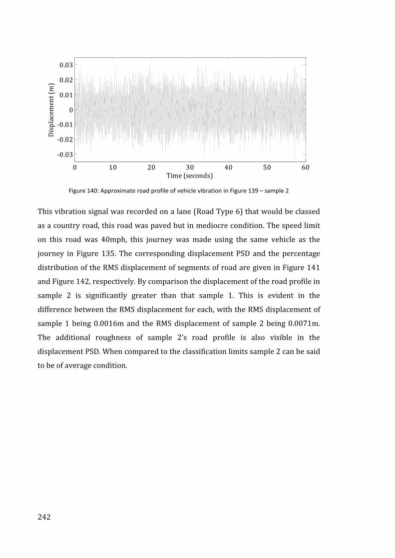
242
0 10 20 30 40 50 60
-0.03
-0.02
-0.01
0
0.01
0.02
0.03
Time (seconds)
Dis
pla
cem
ent
(m)
Figure 140: Approximate road profile of vehicle vibration in Figure 139 – sample 2
This vibration signal was recorded on a lane (Road Type 6) that would be classed
as a country road, this road was paved but in mediocre condition. The speed limit
on this road was 40mph, this journey was made using the same vehicle as the
journey in Figure 135. The corresponding displacement PSD and the percentage
distribution of the RMS displacement of segments of road are given in Figure 141
and Figure 142, respectively. By comparison the displacement of the road profile in
sample 2 is significantly greater than that sample 1. This is evident in the
difference between the RMS displacement for each, with the RMS displacement of
sample 1 being 0.0016m and the RMS displacement of sample 2 being 0.0071m.
The additional roughness of sample 2’s road profile is also visible in the
displacement PSD. When compared to the classification limits sample 2 can be said
to be of average condition.
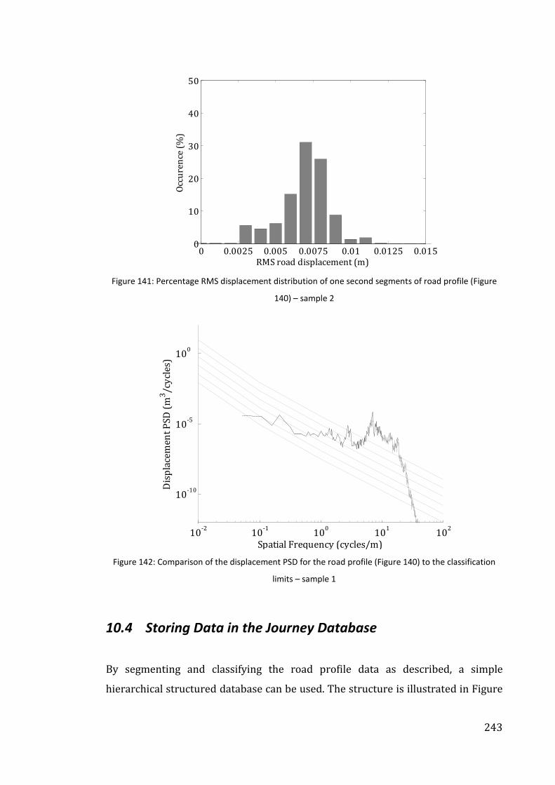
243
0 0.0025 0.005 0.0075 0.01 0.0125 0.0150
10
20
30
40
50
RMS road displacement (m)
Occ
ure
nce
(%
)
Figure 141: Percentage RMS displacement distribution of one second segments of road profile (Figure
140) – sample 2
10-2
10-1
100
101
102
10-10
10-5
100
Spatial Frequency (cycles/m)
Dis
pla
cem
ent
PSD
(m
3/c
ycl
es)
Figure 142: Comparison of the displacement PSD for the road profile (Figure 140) to the classification
limits – sample 1
10.4 Storing Data in the Journey Database
By segmenting and classifying the road profile data as described, a simple
hierarchical structured database can be used. The structure is illustrated in Figure

244
143. This structure allows the user to easily and efficiently select the right road
profile information to use for future journey simulations. The highlighted example
shows the selection of a UK motorway road profile that is in good condition.
America
( N orth )
CountryCountryCountryCountry
User
selects
speed
M ’ way A Roads B Roads Road
road conditionroad conditionroad conditionroad condition
Speed
Very
Good Good
GPS data
Speed
limit
~70mph
etc …….UK
Average Poor Very
Poor
Street/Hill Misc Unclassified
Figure 143: Hierarchical structure of ‘Journey Database’ data classification and storage
10.5 Populating the Journey Database
A method of populating the journey database, which brings together the aspects
discussed in section 10.1, 10.2, 10.3 and 10.4, is illustrated in
Figure 144. This diagram illustrates several key stages in the population process
including:
1. Data collection – vehicle vibration data and the related GPS data is acquired
during in-situ data collection;

245
2. Inverse vehicle model – an approximate road profile is then obtained via an
inverse vehicle model, using the vehicle’s vibration profile as the input;
3. Creating a spatial road profile – by combining the speed profile with the
calculated road profile a spatial approximation of the road profile can be
calculated;
4. Data classification – road profiles are segmented, based on road type e.g.
motorway, A-road, B-road, etc (numerical reference given in Table 29).
These segments are then classified further, based on the road segment’s
condition (numerical reference given in Table 31);
5. Journey database – once classified, the road profiles are stored within the
database from which a simulation journey can be built.
For the purpose of this Thesis a model journey database has been constructed,
using vibration data acquired on home delivery vehicles. The quantity of data
within this model database is given in Table 32, based on road type and condition.
Due to the nature of the distribution journeys data was acquired on, no motorway
data has been collected.
Table 32: Quantity of data available in the model journey database (in minutes)
ROAD TYPE
ROAD CONDITION
1 2 3 4 5 6 7 TOTAL TIME BY ROAD
TYPE (minutes)
1 0 0 0 0 0 0 0 0
2 0 1 2 22 0 0 0 25
3 0 0 0 15 36 0 0 50
4 3 23 37 84 26 0 0 173
5 5 31 101 54 74 2 0 266
6 7 19 120 45 17 0 0 208
7 5 15 4 3 1 0 12 41
Total Time
road condition
(minutes)
19 88 265 223 154 2 12 Total time =
762 minutes

246
Figure 144: ‘Journey Database’ population
247
10.6 Building a Journey
In order to build a journey using the ‘Journey Database’, information on the
intended distribution route is required. This can be achieved using one of the
following options:
Option one: GPS information for the route including speed profile from a previous
journey;
Option two: distribution route map with road speed limits;
Option three: estimates of the distance on each road type with intended speeds.
To enable the use of option one, a programme designed using Matlab was created.
This programme requires the user to input the GPS data from the journey and
produces a breakdown of the time spent on particular road types together with
speed of travel. This method is described by the following steps:
1. GPS data is imported into Matlab, with the address of each GPS point being
found using its longitudinal and lateral co-ordinates.
2. Character recognition is used to identify specific names relating to road types.
3. A numerical value is allocated to each GPS point or journey location based on
the road type.
4. A second numerical value is allocated based on the speed of the vehicle at
each GPS point.
5. An assessment is made as to the severity (roughness) of the road profile
required. This can be done using regional or national statistics on the quality
of roads. ONS (2011a) and ONS (2011b) rate the condition of roads by region
in the UK based on a traffic light scale, where green relates to roads in good
condition and red relates to roads that require maintenance.

248
6. The numerical road type values, selected roughness, along with the distance
are then used to select the appropriate road profile segments to build an
approximate spatial road profile of the journey.
7. The average speed data for each road type segment is then used to convert
the road profile into a displacement time signal, resulting in an approximation
of the distribution journey’s road profile.
Table 33: Speed classifications
SPEED (km/hr) NUMERICAL
VALUE
1 - 5 1
5 – 10 2
10 – 20 3
20 – 30 4
30 – 40 5
40 – 50 6
50 - 60 7
60 – 70 8
70 – 80 9
80 – 90 10
90 - 100 11
100 + 12
Figure 145 illustrates the process of building an approximation of the distribution
journey’s road profile. There are four key stages highlighted in the diagram:
1. Data collection – the GPS data or the journey data is recorded.
2. Journey Evaluation – deconstruct the distribution journey to find the distance
travelled on each road type.
3. Building a journey – the journey evaluation data is then used to select
appropriate road profile segments from the journey database which
approximate the distribution journey’s road profile.
4. Account for speed – using either the speed profile information from the
journey data or speed limits, the spatial road profile approximation is
converted to displacement versus time.

249
Figure 145: Building a journey
10.7 Creating a Vehicle Vibration Approximation
The road profile approximation from section 10.6 can be used as an input into a
quarter vehicle model of the intended distribution vehicle in order to produce an
approximation of the vehicle’s vibration response. Creation of an approximation
of the vehicle’s vibration response is a three stage process, which is described
below and presented schematically in Figure 146.
1. Find or calculate vehicle parameters - The vehicle parameters for the
distribution vehicle need to be found. These are: sprung mass (MV); unsprung
mass (MT); suspension stiffness (KS); suspension damping (CS); tyre stiffness
(KT); and, tyre damping (CT). If the specific vehicle’s parameters are not
directly available, they can be approximated using one of three methods:

250
a. Parameter approximation - using only the vehicle’s sprung mass and
unsprung mass (these are typically specified by the manufacturer), the
remaining vehicle parameters can be approximated using an estimate of
the vehicle’s natural frequencies.
The suspension and tyre stiffness KS and KT can be approximated by
considering each as part of a SDOF mass spring damper system with an
external force, F = 0 and no damping (C = 0). The equation of motion for a
SDOF system can be defined as:
FKxxCxMV =++−...
(53)
where x can be defined as Xe-iωt (Equation 40). By then rearranging
Equation 53, the following relationships for approximating the suspension
and tyre stiffness, can be found:
2
1ωVs MK = and 2
2ωTT MK = (54)
where ω1 = 2πf1 and ω2 = 2πf2 where f1 and f2 are the first and second
natural frequency, these are typically in the ranges 1 – 5 Hz and 10 – 15 Hz,
respectively.
By again considering the free vibration of the system (F = 0), an
approximate value of the suspension damping coefficient (CS) can be found
as the roots of the characteristic equation:
02 =++−M
K
M
Cωω
M
K
M
C
M
C−
±=2
22ω
When ωMMKCC 24 == the system is critically damped. The suspension
damping, CS, can then be defined as:

251
CSVS CKMC ξξ == 4 (55)
where ξ is the damping ratio, with a value between 0 to 1.
Because of the assumptions made when approximating the vehicle
parameters this way, an iterative approach should be used in order to
refine parameter values to ensure sensible results.
b. Vehicle database – Previously used vehicle data that is stored within a
database allows the user to select a representative vehicle. Example
vehicle parameters used in previous studies are given in Table 34. These
parameter values provide a basis for the vehicle database.
For the purpose of this Thesis vehicle parameters have been estimated using
method a, parameter approximation.
2. Build distribution vehicle model – The vehicle parameters are then used to
create a quarter vehicle model in Matlab.
3. Calculate approximation of vehicle vibration response - By running the road
profile through the quarter vehicle model, the approximate vehicle response
can be determined.

252
Table 34: Vehicle model parameters
VEHICLE
QUARTER
TRUCK
(Cebon,
1993)
QUARTER
CAR
(Verros et
al, 2005)
FULL CAR
(Sun and Cui,
2001)
HALF CAR
(Gao et al,
2007)
QUARTER
CAR
(Gobbi et al,
2006)
UPPER-LOWER
LIMITS
(Gobbi et al,
2006)
HALF CAR
(Gopala and
Narayanan,
2008)
HALF SEMI
TRAILER
(Law and Zhu,
2005)
MV (kg) 3,900 375 1,200 1,794.4 229 - 730 3,930 (Cab)
15,700 (Trailer)
MT (kg) 484 60 125 87.15 (Front)
140.4 (Rear) 31 -
40 (Front)
35.5 (Rear)
220 (Front)
1,500 (Middle)
1,000 (Rear)
KS(kN/m) 878 15 50
66.8244
(Front)
18.615 (Rear)
25 0-80 19.96 (Front)
17.5 (Rear)
2,000 (Front)
4,600 (Middle)
5,000 (Rear)
CS (Ns/m) 17,500 1,425 6,000 18,615 1,000
0-5,000 (Passive)
0-700,000
(Active)
1,290 (Front)
1,620 (Rear)
5,000 (Front)
30,000 (Middle)
40,000 (Rear)
KT (kN/m) 1,490 200 400 101.115 120 0-700 175.5 (Front)
175 (Rear)
1,730 (Front)
3,740 (Middle)
4,600 (Rear)
CT (Ns/m) 1,755 7 - - - 0-50,000 -
1,200 (Front)
3,900 (Middle)
4,300 (Rear)
Pitch Inertia (m4) - - 2,100 3,443.05 - - 1,230 -
Roll Inertia (m4) - - 1,800 - - - - -

253
Figure 146: Creating a vehicle vibration approximation
10.8 Concluding Remarks
The journey database has been proposed as a method of creating representative
vehicle vibration profiles, to simulate a specific distribution journey and vehicle.
The three main aspects of the database have been discussed, these are: database
population, data classification and journey simulation.
Three methods of data acquisition were presented. Of these, two methods
allowed the accurate reproduction of the road surface roughness, these were:
using a profilometer and using a inverse quarter vehicle model to approximate
road profile from vehicle vibration.
During this Thesis the inverse vehicle model method has been presented.
Although the method allows the non-Gaussian and non-stationary nature of the

254
road surface roughness to be presented, there are certain limitations pertaining
to the use of the quarter vehicle model. Many of these limitations have been
discussed previously in section 9 and relate to the error in simulating dynamic
parameters as static values and additionally to approximation of these
parameters. In many cases the exact suspension and vehicle dynamics are not
known and therefore an approximation has to be made. The effect of errors, in the
approximation of parameters, on the calculated vehicle response was evaluated in
section 9.6.
The calculated road profiles are stored within the database. To enable simple and
efficient selection, the road profiles are segmented and categorised based on the
road type and condition. Road types are defined through the GPS data from the
journey and the condition of the road is classified based on the displacement PSD
and the RMS displacement distribution.
To then enable the simulation of a journey, either the GPS data or an
approximation of road type and duration is used to assimilate data from the
journey database. By classifying road profiles within the database by severity a
more representative road profile can be built to suit the region of distribution’s
road conditions.
With a road profile approximating the distribution journey, the quarter vehicle
model is used to simulate the distribution vehicle. The inclusion of the vehicle
model enables the consideration of the actual distribution vehicle’s dynamics.
Altogether, this creates a vehicle vibration signal that is representative of the
actual distribution journey and vehicle.
The concept of the journey database has been defined. In order to evaluate its
ability approximate distribution journey vibration accurately, a case study, using
a worked example is required.

255
11 AN IMPROVED TEST REGIME FOR
VIBRATION TESTING OF DISTRIBUTION
PACKAGING
By combining the journey database with the wavelet decomposition method, a
complete test regime for simulating vehicle vibration for the testing of distribution
packaging can be constructed. The process of constructing a simulation using the
improved test regime is illustrated in Figure 147.
User inputted data
Wavelet decomposition method
Journey Database
Identify the distribution journey and vehicle
Including: 1. Vehicle parameters and payload 2. Route information
Construct a representative journey
Build quarter vehicle model
Simulated vehicle vibration
Apply the wavelet decomposition method
Vehicle vibration test simulation
Figure 147: The process of constructing a simulation using the improved test regime

256
There are three key stages involved in the improved test regime, these are:
1. User inputted data – In order to create a test simulation the user must enter
information regarding the distribution journey and vehicle, as explained in
sections 10.6 and 10.7.
2. Journey database – A simulated vehicle response is then constructed using
the journey database, by:
a. Using the journey information to construct an approximation of the
road profile for the distribution journey.
b. The vehicle information is used to construct a quarter vehicle model
of the distribution vehicle, whereby an approximation of the
vehicle’s response to the road profile can be constructed.
3. Wavelet decomposition method – A vibration test simulation is then created
from the approximate vehicle vibration by applying the wavelet
decomposition method.
11.1 Evaluating the Improved Test Regime
The journey database has been proposed as a method of creating a representative
vehicle vibration profile for a given distribution journey and vehicle. In order to
illustrate and evaluate the appropriateness of the journey database an example
database has been used to construct a simulation based on a known distribution
vehicle and journey. Once constructed, this simulation will be compared with a
measured vibration profile from an actual distribution journey. Following this the
wavelet decomposition method will be used to construct a test simulation using
the vehicle vibration produced from the journey database. This will then be
compared to the original vehicle vibration, evaluating the appropriateness of the
improved test regime.

257
11.1.1 Constructing a Simulation Journey
The example distribution journey used in this study is that of a home delivery
journey around parts of Staffordshire and Shropshire, UK. The simulated
distribution journey was then created using vibration data measured on a
distribution journey around Bath, UK. These areas are highlighted on the map
given in Figure 148.
Figure 148: Location of distribution journey and location where journey database data was collected.
The distribution journey being simulated is then illustrated in Figure 149. The
distribution vehicle that was used during the data collection in Bath, UK was a Ford
Luton box van shown in Figure 88. The delivery vehicle used on the home delivery
journey to be simulated was a Ford Transit short wheel base van.

258
Figure 149: Distribution journey around Shropshire and Staffordshire
The vibration profile of the Ford Transit, on the distribution journey given in
Figure 149 is given in Figure 150.
0 500 1000 1500 2000 2500 3000 3500 4000 4500 5000-3
-2
-1
0
1
2
3
Time (seconds)
Acc
erel
atio
n (
g)
Figure 150: Time history vibration profile for Ford Transit van
The GPS data from the distribution journey was analysed using the specially
designed Matlab code. The distance travelled on each of the road classifications
was found, together with the speeds at which the vehicle travelled. This
information is presented in Table 35.

259
Ta
ble
35
: B
rea
k d
ow
n o
f d
istr
ibu
tio
n j
ou
rne
y c
lass
ific
ati
on

260
An approximate distribution journey was then constructed from the journey
database, which contained vibration data from distribution journeys around Bath,
in the Ford Luton box van. Information on the different road segments that were
used to build a distribution journey is given in Table 36 and in Table 42 and Table
43. This information includes the road type, condition, the average expected speed
and the duration of the vibration segment.
Table 36: Road classification of data in journey database
ROAD ROAD
TYPE CONDITION
EXPECTED
SPEED (km/hr)
University 5 Good 32
Bathwick Hill 4 Poor – Heavily potholed 48
City 4 Good 48
Wells Way 4 Average 48
Oldfield Park 5 Good 40
Oldfield Student 5 Average 32
Lower Bristol Road 3 Good 48
NSL (A4) 2 Good 80
Penn Hill Road 4 Good – Traffic calming 48
Weston 3 Poor 48
Royal Cresent 6 Very poor – Cobbled road 32
Lansdown 4 Good 48
Camden 5 Average – Traffic calming 32
Snow Hill 4 Good 32
Into City 4 Good 48
The parameters for both the Ford Luton Box van and the Ford Transit van have
been approximated based on the measured frequency response and manufacturer
quoted vehicle masses. These are given in Table 37, for a quarter vehicle.
Table 37: Approximation of the vehicle parameters
PARAMETER FORD LUTON BOX
VAN (35OL)
FORD TRANSIT
(SWB) VAN
Sprung mass (kg) 604 438
Unsprung mass (kg) 50 45
Suspension Stiffness (kN/m) 149 117
Suspension Damping (kNs/m) 4 3
Tyre Stiffness (kN/m) 387 348

261
The vehicle vibration profile built using the journey database, to approximate the
actual distribution journey, was then inputted into an inverse quarter vehicle
model of the Ford Luton box van, to produce an approximate road profile. This
road profile was then inputted into a quarter vehicle model of the Transit van to
produce a test simulation. The resulting vehicle vibration profile, approximated
from the vehicle model is given in Figure 151.
0 1000 2000 3000 4000 5000 6000-7
-6
-5
-4
-3
-2
-1
0
1
2
3
4
5
6
Time (seconds)
Acc
eler
atio
n (
g)
Figure 151: Simulated vehicle vibration using journey database
11.1.2 Comparison of Results
The overall RMS acceleration, kurtosis, and maximum and minimum acceleration
level for both the original vehicle vibration signal and the simulated signal have
been compared in Table 38. The RMS acceleration of the simulated signal is higher
than the original with 6% error. Additionally, the kurtosis of the simulated signal is
also higher than the original due to the variation in peak accelerations.
Table 38: RMS acceleration, kurtosis and minimum and maximum acceleration levels
Journey RMS
ACCELERATION (g)
Kurtosis,
k
Maximum (g) Minimum
(g)
Original 0.1410 19 4 -2.4
Simulated 0.1489 31 6 -6.4
The RMS acceleration distributions of one second samples for the original and
simulated signal are illustrated in Figure 152. The distribution appears similar,
particularly above 0.15g. This shows good correlation between the two signals.

262
0 0.05 0.1 0.15 0.2 0.25 0.3 0.35 0.4 0.45 0.5 0.55 0.60
5
10
15
20
25
30
35
RMS (g)
Occ
ure
nce
(%
)
Orignal signal
Simulated signal
Figure 152: RMS acceleration distribution for the original signal and simulated signal
In Figure 153, the PSDs for both the original signal and the simulated signal are
also shown to have good correlation.
100
101
102
10-6
10-5
10-4
10-3
10-2
Frequency (Hz)
PSD
(g2
/Hz)
Original Journey
Simulated Journey
ISTA Pick up and delivery vehicle
Figure 153: PSDs for the original signal and the simulated signal
Whilst the simulated signal’s PSD does not match the original signals perfectly, the
overall shape and amplitude is similar. Because of variations in road profiles, the
assumed static vehicle parameters and the constant fluctuations in vehicle speed, it
RMS acceleration (g)

263
would be difficult, if not impossible, to simulate a perfect match in the spectral
shape.
For reference purposes, the PSD provided in the ISTA standards for the vehicle
type relating to that used in this study, has been illustrated on Figure 153. This PSD
shows a much higher frequency component in the low frequency range (1 – 7 Hz)
and overall does not show good correlation to the actual vehicle vibration’s PSD.
11.1.3 Comparison using Wavelet decomposition
The simulated vehicle vibration, created using the journey database, has been
evaluated using the wavelet decomposition method. The simulation signal
produced is illustrated in Figure 154. The signal’s non-stationarity is evident.
0 500 1000 1500 2000 2500 3000 3500 4000 4500 5000 5500 6000-1.5
-1
-0.5
0
0.5
1
1.5
Time (seconds)
Acc
eler
atio
n (
g)
Figure 154: Simulated journey’s wavelet decomposition simulation signal
In Table 38, the signal’s RMS acceleration, kurtosis and maximum and minimum
acceleration levels, are displayed alongside the original signals. The overall RMS
acceleration is similar with only 3.5% error. The simulated signal’s kurtosis
signifies that the signal has a non-Gaussian distribution. The peak acceleration
levels of the simulated signal are lower than the original signal’s, this is due to
averaging when creating the signal.

264
Table 39: RMS acceleration, kurtosis and minimum and maximum acceleration levels
Journey RMS
ACCELERATION
(g)
Kurtosis Maximum
(g)
Minimum
(g)
Original 0.1410 19 4 -2.4
Wavelet decomposition of simulated 0.1460 7.5 1.5 -1.4
The RMS acceleration distribution using one second samples for both signals, is
displayed in Figure 155. It can be seen that the simulated signal’s RMS acceleration
distribution correlated very well with the original signals distribution.
0 0.05 0.1 0.15 0.2 0.25 0.3 0.35 0.4 0.45 0.5 0.55 0.60
5
10
15
20
25
30
35
RMS (g)
Occ
ure
nce
(%
)
Orignal signal
Simulated signal
Figure 155: RMS acceleration distribution of the original signal (Figure 150) and the simulated signal
(Figure 154)
The PSD of the simulated signal has also been compared with the original signal’s
PSD, this is illustrated in Figure 156. Although there is some disparity in the two
spectra, the spectral peaks, in both spectra are similar, therefore the simulated
signal provides a good representation of the original vehicle vibration.
RMS acceleration (g)

265
100
101
102
10-6
10-5
10-4
10-3
Frequency (Hz)
PSD
(g2
/Hz)
Original signal
Simulated signal
Figure 156: PSD of the original signal (Figure 150) and the simulated signal (Figure 154)
11.2 Concluding Remarks
Within this chapter, the improved test regime has been presented and
demonstrated using a case study. The improved test regime includes: the journey
database, which uses both the inverse quarter vehicle model and the quarter
vehicle model; and, the wavelet decomposition simulation method.
In section 11.1.1 the journey database has been used to construct a representative
vibration signal (Figure 151) for the specified distribution journey and vehicle
(Figure 150). The simulated vibration has then been compared to the actual
vibration signal, acquired during the distribution journey. It was found that the
simulated signal match relatively well with the actual vibration signal, showing
good correlation with its PSD and RMS acceleration distribution. This example
therefore proves that the journey database can be used to construct a
representative vibration profile. To further validate the journey database
additional journey simulations are required.
Some discrepancies were seen within the journey database’s simulated vibration
signal. This was due to the presence of some high amplitude shock events within
the journey database data. This could be removed by using lower sampling rates or
filtering signals between a smaller bandwidth (currently 1 – 200 Hz is used).

266
Discrepancies between the actual vehicle vibration and the simulated vibration
signals may also exist due to errors in the approximation of vehicle parameters.
Following the construction of a representative journey, the wavelet decomposition
method was used to create a simulation for laboratory use (Figure 154). This
simulated signal was compared to the original distribution journey (Figure 150)
and was found to correlate well, with the spectral peaks of the simulated signal’s
PSD being at similar frequencies and amplitudes as the actual vehicle vibration’s
spectral peaks. Additionally, the RMS acceleration distribution of the simulated
signal closely matched that of the actual vehicle vibration.
The wavelet decomposition method was also used in section 8.2 and section 8.5 to
construct simulations. In both of these examples the PSD of the simulated vibration
correlated well with that of the original vibration. But, in both examples, the RMS
acceleration distribution of the simulated signal did not correlate as well as the
simulation produced in this example. In both of the previous examples fewer
iterations were carried out during the decomposition, hence a less detailed
decomposition occurred. It is evident from the improvement in the correlation of
the simulated signal in this example with the original signal, that increasing the
number of iterations can improve the accuracy of the simulated signal.

267
12 CONCLUSIONS AND FUTURE
RESEARCH
The aim of this Thesis was to create an improved method for simulating vehicle
vibration for the testing of distribution packaging, with a particular focus on
building a representative test regime generated from an understanding of road
conditions and vehicle dynamics. A key constraint in the formulation of the new
test regime was that the approach used to simulate the vibration must be usable on
all existing laboratory controllers. The need for this research has been highlighted
through the review of current literature and the evaluation of the established
method.
To begin with, a comprehensive description of packaging enabled its importance to
be conceptualised. It was concluded that, for distribution packaging, meeting the
logistical and safety needs of the product/s is vital in creating a successful
packaging solution. This is because distribution packaging not only facilitates
distribution, but also provides the product with the necessary protection from the
distribution environment. To support and expand on this conclusion, a detailed
review of the distribution cycle and all its stages was presented. Vehicle vibration
and shock, during distribution, were highlighted as key contributors to product
damage. With an understanding of the damage potential, an overview of pre-
distribution tests for packaging and the commonly used standards was presented,
covering: drop/impact testing; climatic testing; compression testing; and, vibration
testing.
Combining the protective requirements of the packaging solution with the need for
sustainability, forces the need for the optimisation of packaging. In order to do this
with confidence there is a need for accurate pre-distribution testing of packaging.
Focusing on the specific hazard of vehicle vibration and shock, the key
characteristics of vehicle vibration were defined. This in turn enabled a detailed

268
critique of the established method of pre-distribution vibration testing, identifying
the benefits and limitations of the method. Limitations included: the inaccurate
representation of vehicle vibration as stationary with a Gaussian distribution; the
use of global data to represent all journeys and vehicles; and, using a method of
test acceleration not intended for distribution testing.
To eliminate the limitations of the current method, a review of improved
simulation approaches, suggested in current literature, was carried out. A
correlation study evaluating the ability of each of the approaches to recreate
product damage was also completed. This showed that the modulated RMS
approach correlated most closely with a benchmark time replication vertical
vibration simulation.
The need for MDOF simulation was considered and a case study measuring
product damage was performed. This revealed that in the majority of loading
configurations SDOF testing was adequate.
Alternative methods of signal analysis, using both the time and frequency domain,
were analysed in order to evaluate their ability to capture the characteristics of
vehicle vibration. This analysis highlighted the variation in the frequency content
of the signal over time. The findings from this research were then used to construct
a new and improved simulation method, referred to as wavelet decomposition.
This method was created with the specific intent that it would be usable on
existing laboratory controllers. Therefore the method enables a simulation to be
defined as a series of stationary segments with Gaussian distributions, allowing
each to be simulated from its PSD. When simulated in series, these segments then
create a signal that is non-stationary and has a non-Gaussian distribution.
A correlation study was used to evaluate its effectiveness, with the results of this
study showing that the wavelet decomposition method correlated closely with
time history vertical vehicle vibration.
Following this, focus was drawn to the issue of global data sets in the current
testing standards. A method for constructing a more representative simulation,

269
referred to as, the journey database, was then presented and evaluated in a final
case study.
By combining the wavelet decomposition method with the journey database, a new
improved pre-distribution vibration test regime was created.
The Research Questions developed in section 1.4 and how they have each been
addressed are now considered.
12.1 Research Question 1
How can the effect of a vehicle’s parameters and its journey
conditions on the vehicle’s vibration response be characterised?
Prior to answering this Research Question the characteristics of vehicle vibration
had to be found. In this Thesis, vehicle vibration has been shown to be random,
highly non-stationary and to have a non-Gaussian distribution. With this known,
the first research question could be addressed.
The solution to this problem was to create an improved simulation method using
time-frequency analysis. The method, referred to as wavelet decomposition, uses
the Continuous Wavelet Transform (CWT) to decompose a vehicle vibration signal
in to a number of approximately Gaussian parts (Gaussian approximations).
Each of the Gaussian approximations can then be defined by its PSD and duration.
A simulation signal is then formed by randomly applying each of the PSD for the
corresponding duration. This results in a simulation signal that overall is non-
stationary with a non-Gaussian distribution.
By simulating vehicle vibration using the wavelet decomposition method, the
signal’s non-stationary nature and its non-Gaussian distribution can be simulated,
with the additional advantage, that by simulating each Gaussian approximation

270
based on its PSD, the method is adaptable for: existing controllers; test
acceleration; and, signal averaging.
Three key objectives were set in order to address this Research Question. These
are now discussed.
• Objective 1 - Evaluate current packaging vibration test methods through
comparison with actual vehicle vibration in order to enable the identification of
critical parameters.
To evaluate the current pre-distribution vibration test for packaging, referred to
as the established method, both the techniques used within the method and the
resulting simulation were analysed. Consequently it was shown that, using a
frequency domain analysis technique and subsequently describing vehicle
vibration using the average PSD, false assumptions about the nature and
characteristics of vehicle vibration are made, namely, that it is stationary with a
Gaussian distribution. Further, the method of test acceleration to reduce duration,
which is based on fatigue theory, was also shown to make false assumptions about
the nature of vehicle vibration. These include the assumptions that: it is a single
level vibration; that all components of the packaged product have a single fatigue
rate; and, that product damage is due to fatigue failure and not threshold level
damage.
By then using the established method to simulate vehicle vibration, the resulting
signal differs from the actual vehicle vibration both visually and statistically. The
established method produces a Gaussian signal and therefore the high level
discrete shock events, apparent in actual vehicle vibration, do not appear in the
simulation. Furthermore, the simulated signal is also stationary.
Although the established method made many false assumptions and had
limitations, it use of signal averaging and its allowance for the averaging of
multiple signals, enabled the simulation to have statistical significance.
Furthermore, the established method has gained user confidence through its use
in past testing, and, can be applied to most current laboratory controllers.

271
It was therefore concluded that in order to accurately simulate vehicle vibration,
the simulation technique should account for the signal’s non-stationary and non-
Gaussian nature, whilst still enabling the produced simulation to benefit from
statistical significance and hence confidence in the simulation produced. It was
also deduced that in order to gain user confidence in any new simulation
approach, correlation studies to measure product damage are required.
• Objective 2 – Review improved methods that have been proposed for
vibration simulation in order to establish their benefits and drawbacks.
Improved simulation approaches that have been proposed in previous studies,
were described. These included; time replication; shock on random; two way and
three way split spectra; RMS modulation; and, kurtosis control. It was concluded
that, whilst in theory each of these methods offered improvements on the
established method, in order to fully evaluate their ability to simulate the damage
caused by vehicle vibration, a correlation study using a specific damage
mechanism should be performed.
A case study was carried out to enable a comparison of the level of damage
produced using each approach. The damage mechanism of scuffing was evaluated
and a specially designed rig was used to quantify the damage.
Results from this study showed that the RMS modulation approach correlated best
with the time history simulation. This was an anticipated outcome because the
RMS modulation method enabled the non-stationary and non-Gaussian nature of
the vehicle vibration to be simulated, using the signals statistical distribution.
The use of SDOF testing to simulate the MDOF vehicle movement was evaluated. A
study measuring the damage mechanism of bruising was carried out. The
difference in the level of bruise damage between SDOF and MDOF tests for
different load configurations was measured. Results from this study led to the
conclusion that, in the majority of product load configurations, SDOF vibration
testing along the vertical axis was sufficient for modelling product damage.

272
• Objective 3 - Propose a more realistic test simulation which incorporates the
key characteristics of vehicle vibration.
It is apparent that, in order to simulate vehicle vibration as realistically and
accurately as possible its inherent non-stationarity and non-Gaussian nature
should be accounted for.
The RMS modulation approach appeared to best recreate/match the vehicle
vibration with confidence. It incorporates the RMS acceleration distribution and
hence the signal non-stationarity, and, by creating a simulation signal constructed
from randomly ordered Gaussian signal segments of varying RMS acceleration, is
compatible with existing controllers.
All of the improved simulation methods discussed incorporated Fourier analysis to
evaluate the frequency content of vehicle vibration. By doing this the spectral
shape for the frequency content throughout the signal was constant, based on the
signal average. In reality, as with the signal’s RMS acceleration, the spectral shape
may vary over time.
It was recognised that by using a time-frequency analysis technique, changes in the
spectral shape could be identified. The Short Time Fourier Transform (STFT),
Continuous Wavelet Transform (CWT) and Discrete Wavelet Transform (DWT)
were considered and it was concluded that the CWT was the most appropriate for
use in detecting changes in the spectral shape.
Whilst using wavelet analysis allowed for the spectral shape to be considered, it
did not present a suitable method for creating an overall simulation approach. It
was concluded it was necessary to create a simulation method which was
compatible with existing controllers, which incorporated the benefits of the
established method together with the improved simulation approaches. To ensure
this, the use of Fourier analysis within the simulation method was also required.
With the requirements of the improved simulation approach identified, the
Wavelet decomposition method was then created.

273
The Wavelet decomposition method allows for the RMS acceleration distribution
of the signal to be simulated along with the change in spectral shape. This is
important as certain vibration events may excite different frequencies. By not
simulating the change in spectral content, the additional energy at these
frequencies may be missed and hence any additional damage caused by these
would not be seen during testing.
To evaluate the appropriateness of the Wavelet decomposition method a
correlation study, using the scuffing rig, was carried out. By using this rig the
results from the study could be compared with the previous results, from other
improved simulation approaches.
The result showed that the Wavelet decomposition method correlated well with
time history single axis simulation. In two out of three cases, the Wavelet
decomposition method produced approximately 10-13% more damage than the
time replication. The third case resulted in approximately 8% less damage than
time replication.
By comparison, MDOF simulation created slightly more product damage than
SDOF simulation. Therefore, by using a simulation method that provides a slight
over test in comparison with SDOF time replication, the small amount of additional
damage seen in MDOF vibration can be accounted for.
12.2 Research Question 2
How can the simulation of vehicle vibration for packaging
testing be improved so as to create a more representative test
regime?
It was established that vehicle vibration was caused by the vehicle traversing the
rough road surface. The vehicle’s response was then further characterised by the
vehicle dynamics. The sensitivity of the vehicle’s response to changes in its

274
dynamics resulted in vehicle vibration that is highly variable and unpredictable.
Therefore, in order to define the nature and characteristics of vehicle vibration, the
effect that changes in the vehicle dynamics and the initial road input have on the
measured response, needed to be analysed. Ultimately, this allows the importance
of changes in these parameters to be assessed.
The solution to this Research Question was to create a database of road profile
data, which could be used in conjunction with a quarter vehicle model, of the
intended distribution vehicle, to calculate an approximation of the vehicle
vibration during a specific distribution route.
To build the journey database road profile information was determined from
vehicle vibration data was using an inverse quarter vehicle model. The GPS data,
collected during the vibration data acquisition, was used to segment the road
profiles based on road type. Each road segment could then be further classified by
evaluating its road roughness.
A method for simulating a journey was presented. Whereby, the GPS data for the
intended distribution journey is evaluated in order to estimate the distance
travelled on different road types, including: motorways; A-roads; B-roads; and,
country lanes. Using this information, a road profile can be constructed by
extracting relevant segments of data, stored within the journey database.
Once an approximation of the road profile is constructed, it can be used, along with
the approximate vehicle speed, to simulate the specified vehicle’s vertical vibration
response.
The objectives set to answer this research question are now addressed.
• Objective 4 - Establish the key journey and vehicle parameters that
characterise vehicle vibration and propose a method to account for their
influence on vehicle vibration.
In order to identify the vehicle and journey parameters that shape a vehicle’s
response, a review of previous experimental work that has been reported on in the

275
literature was carried out. Firstly, the road roughness input was evaluated. This
included taking into account: road type; the presence of hazards; and, the
geographical location. Road roughness is not globally consistent, but varies from
country to country and region to region. Furthermore, the presence of hazards was
shown to cause high level shock events in vehicle vibration and the random
occurrence of these events meant that they are highly unpredictable. Road types
and road construction were also shown to affect the road roughness, with asphalt
roads providing a much smoother ride than laterite (unpaved) or concrete roads.
This highlighted the need for the consideration of a distribution journey’s location
and the road types traversed, when creating a simulation test and further
demonstrated the significant error induced by the use of a global data set.
Vehicle parameters that further shape a vehicle’s vibration response were then
considered, including: suspension stiffness and damping; tyre stiffness and
damping; vehicle (sprung) mass; the vehicle unsprung mass; and, payload. The
relationship between variations in these parameters was then further investigated
using a theoretical quarter vehicle model. By analysing these parameters, the
importance of their consideration when simulating a distribution vehicle’s
vibration was made apparent. Seemingly small changes in vehicle parameters
affected the vehicle’s natural frequencies and transmissibility of vibration and
hence ultimately, affected the shape of the vehicle’s response. Incorrect simulation
of the vehicle’s response, may lead to under or over excitation of the packaged
product which consequently, will lead to the inaccurate assessment of damage.
Although the vehicle’s parameters can vary during distribution, static values can
be estimated.
Vehicle speed is another parameter that can greatly affect the severity of the
vehicle’s vibration, where the greater the speed the more severe is the vibration.
Whilst small fluctuations in the vehicle’s speed will occur continuously, the vehicle
average speed can be predicted based on legal speed limits and vehicle speed
restrictions.

276
Whilst all of the parameters so far mentioned can be predicted, the quality of the
driving is not easily determined as this is dependent on individual driver
behaviour.
Finally, with the effect of journey and vehicle parameters determined, the method
by which the vehicle vibration was acquired and measured was then considered. It
was found that vehicle vibration was not consistent across the vehicle floor, with
some locations providing more severe vibration than others. This meant that when
acquiring vehicle vibration, the position at which it is measured must be
considered. Additionally, the method by which the data is acquired, whether
continuously or through sampling, and, the rate at which it is acquired were shown
to affect the measured vibration.
The conclusion was that, whilst an improved simulation method increased the
accuracy of the way in which the vibration was simulated, without consideration of
the intended distribution journey and the distribution vehicle’s parameters, the
confidence in the vibration simulation provided was limited. Therefore, in order to
increase the confidence in the overall improved test regime, consideration of these
parameters must be made.
• Objective 5 - Create a database of vehicle vibration data and propose a
method by which this data can be used to approximate an alternative distribution
journey.
Following the review of vehicle and journey parameters, it was evident that
differences between journeys and vehicles can lead to significant variations in
their vibration responses. This therefore meant that the use of a global data set to
simulate all vehicles and journeys was not appropriate when accuracy in
simulation is required. Because of this, it was decided that in order to create an
overall improved test regime, it was necessary to predict a particular vehicle’s
response and a given distribution journey.
Constraints on time and finance meant that data collection for each distribution
journey was not a viable option. It was therefore decided, that to account for

277
journey variations when simulating vibration, a database of road profile
information that can be used to build a representative road profile for a given
distribution journey would be created. The journey database provided a method
that was not time consuming through reducing the amount of data acquisition
required.
The database was populated using an inverse quarter vehicle model to
approximate road profiles from a given vehicle’s measured vibration. The
approximate road profile of a journey was then segmented using the GPS data from
the journey on which the vibration was acquired. This enabled the road profile to
categorise based on the road type. These road profile segments were then further
classified by measuring each segments road roughness.
This meant that when considering the vehicle vibration for a given distribution
journey and vehicle a representative vehicle vibration could be calculated using a
quarter vehicle model and a road profile built to approximate the distribution
journey.
• Objective 6 - Create an improved test regime with an integrated vehicle
model which allows for the established variations in vehicle and journey
parameters to be considered.
Whilst the journey database enabled the creation of a road profile to approximate
the intended distribution journey, a computational quarter vehicle model was then
enabled the simulation of the intended distribution vehicle’s vibration response.
This enabled the vehicle parameters for a particular distribution vehicle to be
considered.
The journey database and vehicle model, together with the wavelet decomposition
method, have provided an overall improved test regime. This enabled the
construction of representative vehicle vibration simulations, improving the
accuracy of the established method’s simulation approach and data selection.
A case study was carried out, whereby, a given distribution vehicle’s vibration on a
given distribution route was simulated using the improved test regime. Firstly, the

278
journey database was used to construct an approximate vehicle vibration based on
the distribution vehicle and the GPS data of the distribution route. The
approximated vehicle’s vibration was compared to the actual measured vibration
signal and showed good correlation, matching well the actual vehicle’s RMS
acceleration distribution and average PSD.
A simulation was then produced using the wavelet decomposition method and the
journey database’s approximated vehicle vibration. The simulation also correlated
well with the actual vehicle vibration.
This study showed that the improved test regime could be used to simulate a given
distribution journey and vehicle.
12.3 Contribution to Knowledge
This Thesis has presented a new and improved method for simulating vehicle
vibration for the pre-distribution testing of packaging. This test regime consists of
two major components:
• The journey database
The journey database allows for the creation of a simulation that is representative
of a given distribution journey and vehicle. Both the method of populating the
database and the method of creating a journey have been presented.
1. Populating the journey database:
a. An inverse quarter vehicle model has been developed so that the road
profile for a given vehicle vibration, can be approximated.
b. Road profiles are segmented using the journey’s GPS data to identify
changes in road type e.g. motorway, A-road, B-road, etc.
c. The displacement PSD relating to each road profile segment is then
used to classify the segment’s roughness severity.

279
2. Building a simulation journey:
a. Deconstructing the intended distribution journey to identify the
distance travelled on each road type.
b. Constructing an approximate road profile from the journey database,
based on the intended journey’s road types and severity.
c. Calculate an approximate vehicle vibration for the intended journey
and vehicle, using a quarter vehicle model of the distribution vehicle
and the approximate road profile.
• The wavelet decomposition method
The wavelet decomposition method allows the representative vehicle vibration,
calculated from the journey database, to be converted into a test simulation.
Wavelet analysis is used to decompose a signal into a series of Gaussian
approximations. By randomly simulating each approximation using its PSD and
duration, a simulation signal can be created. Similar to vehicle vibration, the
simulated signal is non-stationary with a non-Gaussian distribution. By
constructing the simulation from Gaussian segments, and simulating only the
vertical vibration, the wavelet decomposition method meets the key constraints
associated with existing controllers.
Vehicle vibration is highly non-stationary and has a non-Gaussian distribution.
Therefore, applying the wavelet decomposition method will inevitably result in
one segment that is highly non-stationary and has a non-Gaussian distribution.
This segment will contain the vibration signal’s high amplitude shock events. To
ensure the wavelet decomposition method is usable for all existing controllers, this
segment must be assumed to be stationary and to have an approximately Gaussian
distribution, allowing it to be simulated from its PSD. This assumption means that
the extreme high level shock events present within this segment will be averaged
out and therefore not simulated. This is the main limitation of the wavelet
decomposition method.

280
It should be noted that, because the wavelet decomposition method allows a signal
to be decomposed into relatively small segments, the effect of averaging on the
intensity of each segment will be significantly less than the effect of averaging on
the existing method, where averaging is applied to the signal as a whole.
A further benefit of the wavelet decomposition method is that it allows for test
acceleration, by accelerating the PSD of each segment, removing the need for long
and arduous simulations.
12.4 Future Research
Several areas of future research have been highlighted. These include:
1. To further build confidence in the overall test regime further experimental
work is required.
2. In order to create a more concise and complete journey database and to allow
the more accurate creation of an approximate road profile, further data is
required.
3. As tri-axial and multi-axial simulation tables become more readily available, it
may be more appropriate to simulate vehicle vibration in more than one axis.
Therefore, further work evaluating the need for MDOF and how it should be
implemented within the test regime, would be required. This includes the
implications for the vehicle model and how these would be addressed.
5. In addition, the desirability of test acceleration to reduce test duration, points
to the need for evaluation of a suitable method of test acceleration that can be
applied to the wavelet decomposition method. Each of these aspects is now
discussed.

281
12.4.1 Further Experimental Work
The ability of both the wavelet decomposition method and the journey database to
create improved simulations has been shown through case studies. In order to
present a rounded view of the work a case study evaluating both in tandem is
required.
Additional correlation studies using products each with a known overriding
damage mechanism, should be carried out in order to further demonstrate the
accuracy of the wavelet decomposition method and thereby build confidence in the
technique.
12.4.2 Additional Data Acquisition
The current journey database is very limited and can therefore only be used to
simulate distribution journeys within the UK that are carried out on limited road
types and conditions. Therefore, in order to allow for more accurate
representations of distribution journeys a more comprehensive journey database
is required. Therefore further data acquisition is required to populate the journey
database, this should include road profile data from different regions and
countries, to account for variations in geographical locations.
12.4.3 The use of MDOF Simulation
The use of MDOF simulation has been discussed and evaluated in this Thesis. The
conclusions were that SDOF simulation was sufficient to evaluate product damage
during distribution, as long as products were packed in a uniform, stable
configuration. The restriction of many existing controllers to the use of single axis
testing has been a cause of limitation to the method of simulation. But, with
increase in tri-axial and multi-axial simulation rigs, the option for MDOF testing is
becoming more viable. Therefore, further research into the effect of MDOF
vibration, simulating different combinations of axes e.g. tri-axial or vertical, pitch

282
and roll, would be beneficial in the further development of the simulation test
regime.
The addition of MDOF testing also requires the evaluation of the Wavelet
decomposition method in a multi axial configuration, and additionally, the
consideration of how the multi axial vibration data is measured when calculated
using the journey database and vehicle model.
A further requirement is the need to create a full vehicle model so that all axes can
be simulated. This brings with it further complications such as additional
parameter information requirements, such as: vehicles inertia and mass
distribution.
12.4.4 Development of the Computational Vehicle Model
It has been mentioned that the use of MDOF vibration simulation would require
the development of a full vehicle model.
Additionally, the quarter vehicle model could be further developed. This would
allow for a more accurate simulation of the intended vehicle. This might include
accounting for: tyre and suspension dynamics and variation, or, load fluctuations;
this would increase the accuracy of the simulated vehicle vibration.
12.4.5 The use of Accelerated Testing
The established method uses test acceleration based on fatigue theory (section
4.1). The use of this method for accelerating the wavelet decomposition method
needs to be examined. Additionally, alternative methods of test acceleration should
also be evaluated, with damage correlation studies used to evaluate their
appropriateness. Some examples of alternative test acceleration methods are now
given.
• Use only the most severe amplitudes observed, hence cutting out some of the
testing duration

283
Vibration, below a certain amplitude, is assumed to cause negligible damage to the
specimen and therefore can be removed from the test profile so as to reduce
duration. This may seem a valid way of reducing test duration, but it does not
consider the effects that the low amplitude vibration may have on the specimen
once it has been damaged or ‘compromised’ by the high level vibration.
In future work this assumption should be tested using correlation studies in its
evaluation.
• Find the conditions which lead to rapid damage and test at those levels, this
again removes some of the test duration
This is similar to that of the sine sweep test. The specimen is subjected to the range
of frequencies from the measured environment at which it resonates for an
extended period of time. This could be done by locating the frequency range over
which the transmissibility is greater than one, creating a test simulation using only
frequencies in that range.
This method of test acceleration would lead to an unrealistic simulation, since it
subjects the specimen to the worst possible conditions it could experience, for an
extended period of time. In reality, it may only be subject to such conditions for a
very limited amount of time and hence, its effect would not be so great.
• Increase the frequency of the applied vibrations, hence 'compacting' the test.
Farrar et al (1999) gives the following example of the use of this method ‘…a
component subjected to a low-frequency shipboard vibration environment say 20 H.
sinusoidal. If the first mode of the component of interest were, for example, 300 Hz,
then, depending on damping, an increase of a factor of 10 in the test frequency,
without an amplitude change, would reduce the total test time by the same factor.
Increasing the magnitude of the input signal appropriately could be used to further
compress the test time….’
‘Increasing vibration amplitude above the normal levels leading to a reduction in
testing time’ and ‘Use only the most severe amplitudes observed, hence cutting out

284
some of the testing duration’, are the most viable methods, as they both accelerate
the tests whilst still providing a semi realistic simulation of the distribution
environment. Both of these would need comparison with real-time simulation to
see how accurate they are for use.

285
APPENDIX I. PUBLICATIONS RESULTING
FROM THIS WORK
I.I. Journal Articles
K. Griffiths, D. Shires, W. White, Prof. P. S. Keogh, Dr B. J. Hicks (2012) Correlation
Study Using Scuffing Damage to Investigate Improved Simulation Techniques for
Packaging Vibration Testing. Packaging, Technology and Science. published online:
2nd July 2012
I.II. Conference Papers
K. R Griffiths, B. J. Hicks, P. S. Keogh, D. Shires (2010) Investigating the Suitability of
Testing Standards for Simulating Vehicle Vibrations during Supermarket Home
Delivery. 17th IAPRI World Conference on Packaging. Tianjin, China. October 12th -
16th
K. R Griffiths , P. S. Keogh, B. J. Hicks (2011) Simulating the Transport Environment
for Packaging Testing Using a Multi Degree of Freedom Method. ISTA Transport
Packaging Forum 2011. Florida, USA. April 18th-21st

286
13 APPENDIX II. REFERENCES
AASHTO (2009) Rough Roads Ahead: Fix it Now or Pay for it Later [Online].
Available: http://roughroads.transportation.org/RoughRoads_FullReport.pdf.
[Accessed: 8th September 2012].
Addison, P. (2002) The Illustrated Wavelet Transform Handbook. IoP Publishing
Ltd. (Accessed 22nd May 2012).
Adeli, H., Z. Zhou & N. Dadmehr (2003) Analysis of EEG Records in an Epileptic
Patient using Wavelet Transform. Journal of Neuroscience Methods, 123, 69 - 87.
Akansu, A. & R. Haddad (2001) Multiresolution Signal Decomposition: Transforms,
Subbands, Wavelets: Transforms, Subbands, and Wavelets. Elsevier Academic Press.
London, UK.
Association for Safe International Road Travel (ASIRT) (2004) Road Travel Report
India [Online]. Available: www.asirt.org.
ASTM (2006) Standard Practice for Performance Testing of Shipping Containers
and Systems ASTM D4169 – 09. Philadelphia, USA: ASTM.
Azzi, A., D. Battini, A. Persona & F. Sgarbossa (2012) Packaging Design: General
Framework and Research Agenda. Packaging, Technology and Science. Online 31st
January 2012
Bai, R. (2010) Lenovo Packaging Specification 45J5387 - Packaging Cosmetic
Requirements. Lenovo Corporation
Barchi, G. L., A. Berardinelli, A. Guarnieri, L. Ragni & C. T. Fila (2002) Damage to
Loquats by Vibration-simulating Intra-state Transport. Biosystems Engineering, 82,
305 - 312.

287
Barling, D., R. Sharpe & T. Lang. (2008) Re-Thinking Britain's Food Security
[Online]. Available: http://www.soilassociation.org/. The soil Association.
[Accessed: 10th June 2012].
Basquin, O. H. (1910) The Exponential Law of Endurance Testing. Proceedings of
American Society for Testing and Materials, 19, 625 - 630.
Bech-Larsen, T. (1996) Danish Consumers' Attitudes to the Functional and
Environmental Characteristics of Food Packaging. Journal of Consumer Policy, 19,
339 - 363.
Berardinelli, A., V. Donati, A. Giunchi, A. Guarnieri & L. Ragni (2004) Damage to
pears caused by simulated transport. Journal of Food Engineering, 66, 219 - 226.
Bernad, C., A. Laspalas, D. Gonzalez, E. Liarte & M. A. Jimenez (2010) Dynamic
Study of Stacked Packaging Units by Operational Modal Analysis. Packaging,
Technology and Science, 23, 121 - 133.
Bernad, C., A. Laspalas, D. Gonzalez, L. Nunez & F. Buil (2011) Transport Vibration
Laboratory Simulation; On the Necessity of Multiaxis Testing. Packaging,
Technology and Science, 24, 1 - 14.
Bhave, S. (2010) Mechanical Vibrations Theory and Practice. India: Dorling
Kindersley.
Bogsjo, K. (2006) Development of Analysis Tools and Stochastic Models of Road
Profiles Regarding Their Influence on Heavy Vehicle Fatigue. Vehicle System
Dynamics: International Journal of Vehicle Mechanics and Mobility, 44, 780 - 790.
Bogsjo, K., K. Podrorski & I. Rychlik (2012) Model for Road Surface Roughness.
Vehicle System Dynamics, 50(5), 725 - 747
Boonruang, K., V. Chonhenchob, S. P. Singh, W. Chinsirikul & A. Fuongfuchat (2012)
Comparison of Various Packaging Films for Mango Export. Packaging, Technology
and Science, 25, 107 - 118.

288
Brundtland. (1987) Our Common Future: the report on the World Commission on
Environment and Development. Oxford: The Brundtland Commission.
Bruscella, B., V. Rouillard, & M. Sek (1999) Analysis of Road Surface Profiles.
Journal Transport Engineering, 125(1), 55 – 59.
BS7853 (1996) Mechanical Vibration: Road Surface Profiles Reporting of Measured
Data. British Standards. BS 7853:1996
Cabinet Office Strategy Unit (COSU) (2008) Food Matters Towards a Strategy for
the 21st Century [Online]. Available: http://www.cabinetoffice.gov.uk-
/strategy/work_areas/food_policy.aspx.
Carter, C. R. & D. S. Rogers (2008) A framework of sustainable supply chain
management: moving toward new theory. International Journal of Physical
Distribution and Logistics Management, 38 (5), 360 – 87.
Cebon, D. (1999) Handbook of Vehicle-Road Interaction. lisse, Abingdon. Swets &
Zeitlinger
Cheng, C. & D. Cebon (2008) Improving Roll Stability of Articulated Heavy Vehicles
using Active Semi-Trailer Steering. Vehicle System Dynamics, 46, 373 - 388.
Chonhenchob, V., S. P. Singh, J. J. Singh, J. Stallings & G. Grewal (2012) Measurement
and Analysis of Vehicle Vibration for Delivering Packages in Small-Sized and
Medium-Sized Trucks and Automobiles. Packaging, Technology and Science, 25, 31
- 38.
Chonhenchob, V., S. Sittipod, D. Swasdee, P.Rachtanapun, S. P. Singh & J. Singh
(2009) . Effect of Truck Vibration during Transport on Damage to Fresh Produce
Shipments in Thailand. Journal of Applied Packaging Research, 3 (1), 27 - 38.
Coles, R. & M. J. Kirwan (2011) Food and Beverage Packaging Technology. Blackwell
Publisher Ltd.

289
Council of Logistics Management (CLM) (1998) What's it All About?. Oak Brook, IL,
USA.
Daubechies, I. (1990) The Wavelet Transform, Time-frequency Localization and
Signal Analysis. IEEE Transaction on Information Theory. 23 (5) 961 - 1005
Daubechies, I. (1992) Ten Lectures on Wavelets. CBMS-NSE Regional Conference
Series. Capital City Press.
Department for Environment, Food and Rural Affairs. (DEFRA) (2011) Food
Statistics Pocketbook [Online]. Available: http://www.defra.gov.uk/statistics-
/files/defra-stats-foodfarm-food-pocketbook-2011.pdf. York, UK. [Accessed: 23rd
July 2012].
Department for Transport (DfT) (2012) Prevention and a Better Cure: Potholes
Review [Online]. Available: http://www.dft.gov.uk/publications/pothole-review/.
London, UK. [Accessed: 15th September 2012].
Department for Transport (DfT) (2010) Road Lengths (miles) by Road Type and
Region and Country in Great Britain, Annual. London, UK.
Ek, M., G. Gellerstedt & G. Henriksson (2009) Paper Products Physics and
Technology. Pulp and Paper Chemistry and Technology.
ERM (2003) Environmental Resources Management, Streamlined LCA study of
apple packaging systems. Marks & Spencer Plc.
EUROPEN (2009) Packaging in the Sustainability Agenda: A Guide for Corporate
Decision Makers. EUROPEN.
EUROSTAT (2008) Packaging waste data 2008, 1000 tonnes. Statistical Office of
the European Union. [Accessed: 10th June 2012].
FAO (2004) Globalization of Food Systems in Developing Countries: Impact on
Food Security and Nutrition. In FAO Food and Nutrition Paper. Rome.
290
Farrar, C. R., T. A. Duffey, P. J. Cornwell & M. T. Bement (1999) A Review of Methods
for Developing Accelerated Testing Criteria. Proceedings of the 17th International
Modal Analysis Conference, 3727, 608
Gabor, D. (1945) Theory of Communication, Part I: The Analysis of Information.
Journal of the Institution of Electrical Engineers - Part III: Radio and Communication
Engineering, 93 (26), 429 - 441
Garcia-Romeu-Martinez, M.-A., S. P. Singh & V.-A. Cloquell-Ballester (2008)
Measurement and Analysis of Vibration Levels for Truck Transport in Spain as a
Function of Payload, Suspension and Speed. Packaging Technology and Science, 21,
439 - 451.
Garcia-Romeu-Martinez, M. A. & V. Rouillard (2011) On the Statistical Distribution
of Road Vehicle Vibrations. Packaging, Technology and Science, 24, 451 - 467.
Garret, T. K., W. Steeds & N. Newton (2001) The Motor Vehicle. Elsevier
Butterworth-Heineman.
Gillespie, T. D. (1985) Measuring Road Roughness and its Effects on User Cost and
Comfort. American Society for Testing and Materials. (Accessed: 1th June 2012).
Goodwin, D. & D. Young (2011) Protective Packaging for Distribution. Pennsilvania,
USA. DEStech Publications, Inc.
Hanlon, J. F., R. J. Kelsey & H. E. Forcinio (1998) Handbook of Package Engineering.
Technomic Publishing Company, Inc.
Harrison, M. (2004) Vehicle Refinement: Controlling Noise and Vibration in Road
Vehicles. Oxford, UK: Butterworth-Heinemann.
Hartley, L. R., P. K. Arnold (1994) Indicators of Fatigue in Truck Drivers. Applied
Ergonomics, 25(3), 143 - 156.
Hellstrom, D. & M. Saghir (2007) Packaging and Logistics Interactions in Retail and
Supply Chains. Packaging, Technology and Science, 20, 197 - 216.

291
IEA (2003) IEA Triennial Report, 2001-2003. Santa Monica, CA, USA.
INCEPN (2008) Packaging in Perspective, Advisory Committee on Packaging.
INCEPN.
ISO (2008) ISO BS EN 60068-2-6: Environmental Testing. In Part 2-6: Tests – Test
Fc: Vibration (Sinusoidal).
ISO (2009) ISO 11228 Ergonomics. Manual Handling. In Part 3: Handling of low
loads at high. ISO.
ISO (2009b) ISO 11228. Ergonomics. Manual Handling. In Part 2: Pushing and
pulling. ISO.
ISO (2009c) ISO 11228. Ergonomics. Manual Handling. In Part 1: Lifting and
carrying. ISO.
ISTA (2012) Guidlines for Selecting and Using ISTA Test Procedures and Projects.
East Lansing, Michigan, USA.
ISTA (2010) Resource Book 2010. East Lansing, MI, USA.
Jalili, N. (2002) The Mechanical Systems Design Handbook Modelling, Measurement
and Control; Chapter 12: Semi-Active Suspension Systems. USA. CRC Press LLC.
Jarimopas, B., S. P. Singh & W. Saengnil (2005) Measurement and Analysis of Truck
Transport Vibration Levels and Damage to Packaged Tangerines during Transit.
Packaging Technology and Science, 18, 179 - 188.
Jing, L. & Q. Liangsheng (2000) Feature Extraction Based on Morlet Wavelet and its
Application for Mechanical Fault Diagnosis. Journal of Sound and Vibration, 234,
135 - 148.
Joint Industry Unsaleables Steering Committee (JIUSC) (2006) 2006 Unsaleables
Benchmark Report. http://www.gmaonline.org.

292
Kenco (2012) Terracycle - Out Smart Waste [Online]. Available: http://www-
.terracycle.co.uk/en-UK/brigades/the-kenco-eco-refill-brigade-r.html. [Accessed:
10th July 2012].
Kipp, W. I. (2000) (updated 2008). Vibration Testing Equivalence - How Many
Hours of Testing Equals How Many Miles of Transport. In ISTA Conference 2000.
ISTA.
Kipp, W. (2001) Accelerated Random Vibraiton With Time history Shock for
improved Laboratory Simulation. In IoPP Annual Members Meeting. San Jose,
California.
Kipp, W. (2008a) Environmental Data Recording, Analysis and Simulation of
Transport Vibrations. Packaging, Technology and Science, 21, 437 - 438.
Kipp, W. (2008b) Random Vibration Testing Of Packaged-Products: Considerations
For Methodology Improvement. In IAPRI World Conference on Packaging. Bangkok,
Thailand. ISTA.
Koojiman, J. (2000) Environmental impact of packaging – performance in the
household.
Law. S. S. & X.Q. Zhu (2005) Bridge dynamic responses due to road surface
roughness and braking of vehicle. Journal of Sound and Vibration. 282. 805 – 830.
Leemans, V., H. Magin, M. F. Destain, (2002) On-line fruit grading according to their
external quality using machine vision. Biosystems Engineering. 83, 397 – 404.
Levy, G. M. (1999) Packaging, Policy and Environment. Aspen Publishers Inc.
Liew, K. M. & Q. Wang (1998) Application of Wavelet Theory for Crack
Identification in Structures. 124, 152 - 157.
Lin, J. (2001) Feature Extraction of Machine Sound Using Wavelet and its
Application in Fault Diagnosis. NDT & E International, 34.

293
Lu, F., Y. Ishikawa, H. Kitazawa & T. Satake (2010) Effect of Vehicle Speed on Shock
and Vibration Levels in Truck Transport. Packaging, Technology and Science, 23,
101 - 109.
Lu, F., Y. Ishikawa, T. Shiina & T. Satake (2008) Analysis of Shock and Vibration in
Truck Transport in Japan. Packaging Technology and Science, 21, 479 - 489.
Lutes, L. D. & S. Sarkani. (2004) Random Vibrations: Analysis of Structural and
Mechanical Systems. Oxford, UK: Butterworth-Heinemann.
Macdonald, J. (1994) Quality in Retail and Distribution. The TQM Magazine, 6, 11 -
14.
Mallat, S. (1999) A Wavelet Tour of Signal Processing. Elsevier Academic Press.
Marsh, K. & B. Bugusu (2007) Food Packaging - Roles, Materials and Environmental
Issues. Journal of Food Science 72, 39 - 55.
Marsh, K. S. (1997) The Wiley Encyclopaedia of Packaging Technology. 2nd Edition.
Wiley. New York, USA.
Meyers, H. M. & M. J. Lubliner. (1998) The Marketer's Guide to Sucessful Packaging
Design. Chicago, usa. NTC Business Books.
Miege, A. J. P. & D. Cebon (2005) Optimal Roll Control of an Articulated Vehciel:
Theory and Model Validation. Vehicle System Dynamics, 43, 867 - 893.
Mintel (2012) Food and Drink Packaging Trends - UK, January 2012. London, UK.
MoD (1999) Defence Standard 00-35, Part 5: Induced Mechanical Environments;
Ministry of Defence
Nei, D., N. Nakamura, P. Roy, T. Orikasa, Y. Ishikawa, H. Kitazawa & T. Shiina (2008)
Wavelet Analysis of Vibration and Shock on the Truck Bed. Packaging, Tehcnology
and Science, 21, 491 - 499.

294
Newland, D. E. (1994) An Introduction to Random Vibrations, Spectral and Wavelet
Analysis. England: Longman Scientific and Technical.
OECD. (2002) Transport Logistics: Shared Solutions to Common Challenges. OECD.
Office of National Statistics (ONS) (2011a). Percentage of Unclassified Roads
Where Maintenance Should be Considered by Region, England: 2006/06 to
2010/11. Department for Transport. London, UK.
Office of National Statistics (ONS) (2011b). Road Condition Indicator (RCI) Scores
by Percentage of Classified Roads, by Local Authority, England: 2006/07 to
2010/11. Department for Transport. London, UK.
Olorunda, A. O. & M. A. Tung (1985) Simulated Transit Studies on Tmatoes; Effects
of Compressive Load, Container, Vibration and maturity on Mechanical Damage.
International Journal of Food Science and Technology, 20, 669 - 678.
Otari, S., S. Odof, J. B. Nolot, P. Vasseur, J. Pellot, N. Krajka & D. Erre (2011)
Statistical Characterization of Acceleration Levels of Random Vibrations during
Transport. Packaging, Technology and Science, 24, 177 - 188.
Pacejka, H. B. (2006) Tyre and Vehicle Dynamics. 2nd Edition. Oxford, UK.
Butterworth-Heinemann.
Paine, F. A. & Paine, H. Y. (1992) A Handbook of Food Packaging. Blackie Academic
and Professional.
Paull, R. E. (1999) Effect of Temperature and Relative Humidity on Fresh
Commodity Quality. Postharvest Biology and Technology, 15(3), 263 - 277.
Peleg, K. (1985) Produce-handling, Packaging and Distribution. Haifa, Israel:
Department of Argicultural Engineering Technology.
Philip, P., J. Taillard, M. A. Quera-Salva, B. Bioulac & T. Akerstedt (1999) Simple
Reation Time, Duration of Driving and Sleep Deprivation in Young Versus Old
Automobile Drivers. Journal of Sleep Research, 8, 9 - 14.

295
Pilditch, J. (1972) The Silent Salesman. London: Business Books Ltd. Packaging
Systems. Environmental Resources Management.
Piringer, O. G., Baner, A. L. (2008) Plastic Packaging: Interactions with Food and
Pharmaceuticals. 2nd Edition. Wiley.
Pollock, D. S. G. (1999) Handbook of Time Series Analysis, Sisgnal Processing and
Dynamics. Elsevier.
Rajamani, R. (2012) Vehicle Dynamics and Control. 2nd Edition. New York, USA:
Springer.
Ramji, K., A. Gupta, V. H. Saran, V. K. Goel & V. Kumar (2004) Road Roughness
Measurements Using PSD Approach. Journal of the Institution of Engineers (India),
85, 193 - 201.
Rao, T., G. Rao, K. Rao & A. Purushottam (2010) Analysis of Passive and Semi Active
Controller Suspension Systems for Ride Comfort in an Omnibus Passing Over a
Speed Bump. International Journal of Research and Reviews in Applied Sciences, 5.
Richards, D. P. (1990) A Review of Analysis and Assessment Methodologies for
Road Transportation Vibration and Shock Data. Environmental Engineering, 3.
Riverford (2012) Packaging [Online]. Available: http://www.riverfordenviron-
ment.co.uk/. [Accessed: 16th June 2012].
Robinson, G. (2006) Globalization of the Packaging Supply Chain. In Dimensions 06.
San Antonio, Texas: ISTA.
Rouillard, V. (2007a) On the Non-Gaussian Nature of Random Vehicle Vibrations.
In Proceedings of the World Congress on Engineering. London, UK.
Rouillard, V. (2007b) The synthesis of road vehicle vibrations based on the
statistical distribution of segment lengths. In 5th Australasian Congress on Applied
Mechanics. Brisbane, Australia.

296
Rouillard, V. (2008) Generating Road Vibration Test Schedules from Pavement
Profiles for Packagin Optimization. Packaging Technology and Science, 21, 501 -
514.
Rouillard, V. & M. Lamb (2008) On the Effects of Sampling Parameters When
Surveying Distribution Vibrations. Packaging Technology and Science, 21, 467 -
477.
Rouillard, V. & M. Sek (2010) Synthesizing Nonstationary, Non-Gaussian Random
Vibrations. Packaging, Technology and Science, 23, 423 - 439.
Rouillard, V. & M. A. Sek (2000) Monitoring and Simulating Non-stationary
Vibrations for Package Optimization. Packaging Technology and Science, 13, 149 -
156.
Rouillard, V. & M. A. Sek (2001) Simulation of Non-Stationary Vehicle Vibrations.
Proceedings of the Institution of Mechancial Engineers - Part D - Journal of
Automobile Engineering, 215(10), 1069 - 1075.
Rouillard, V. & M. A. Sek (2005) The Use of Intrinsic Mode Functions to
Characterise Shock and Vibration in the Distribution Environment. Packaging
Technology and Science, 18(1), 39 - 51.
Rushton, A., P. Croucher & P. Baker. (2010) The Handbook of Logistics and
Distribution Management. Kogan Page Limited.
Sahambi, J. S. (1997) Using Wavlet Transforms for ECG Characterization, An on-line
Digital Signal Processing System. Engineering in Medicine and Biology Magazine,
16, 77 - 83.
Sainsburys, First Full Range of Milk Bags to Hit UK Supermarkets [Online].
Available: http://www.j-sainsbury.co.uk/media/latest-stories/2010/20100811-
first-full-range-of-milk-bags-to-hit-uk-supermarkets/. [Accessed: 28th August
2012].

297
Saskatchewan Highways and Transportation (SHT) (2001) Standard Test
Procedures Manual [Online]. Available: http://www.highways.gov.sk.ca-
/indexstp/.
Sek, M. A. (1996) A modern technique of Transportation Simulation for Package
Performance Testing. Packaging Technology and Science, 9, 327 - 343.
Shiavi, R. (2007) Introduction to Applied Statistical Signal Analysis: Guide to
Biemedical and Electrical Engineering Applications. Third Edition. Elsevier, 201 -
228
Shires, D. (2011) On the time compression (test acceleration) of broadband
random vibration tests. Packaging Technology and Science, 4, 75 - 82.
Shires, D. & W. White. 2011. The Comparison of Different Vibration Test
Methodologies. In Transport Packaging Forum, ed. ISTA. Florida, USA: ISTA.
Singh, B. N. & A. K. Tiwari (2006) Optimal Selection of Wavelet Basis Function
Applied to ECG Signal Denoising. Digital Signal Processing, 16, 257 - 287.
Singh, J., S. P. Singh & E. Joneson (2006) Measurement and Analysis of US Truck
Vibration for Leaf Spring and Air Ride Suspension and Development of Tests to
Simulate These Conditions. Packaging, Technology and Science, 19, 309 - 323.
Singh, S. P., J. R. Antle & G. G. Burgess (1992) Comparison Between Lateral,
Longitudinal and Vertical Vibration Levels in Commercial Truck Shipments.
Packaging, Technology and Science, 5, 71 - 75.
Singh, S. P., E. Joneson, J. Singh & G. Grewal (2008) Dynamic Analysis of Less-than-
truckload Shipments and Test Method to Simulate This Environment. Packaging
Technology and Science, 21, 453 - 466.
Singh, S. P., A. P. S. Sandhu, J. Singh & E. Joneson (2007) Measurement and Analysis
of Truck and Rail Shipping Environment in India. Packaging Technology and
Science, 20, 381 - 392.

298
Singh, S. P. & M. Xu (1993) Bruising in Apples as a Function of Truck Vibration and
Packaging. Applied Engineering in Agriculture, 9, 455 - 460.
Skills (2008) UK Trade performance: Patterns in UK and Global Trade Growth. In
BIS Economics Paper No. 8.
Smith, A., P. Watkiss, G. Tweddle, A. McKinnon, M. Browne, A. Hunt, C. Treleven, C.
Nash & S. Cross. (2005) The Validity of Food Miles as an Indicator of Sustainable
Development. DEFRA. http://archive.defra.gov.uk/evidence/economics/foodfarm-
/reports/documents/foodmile.pdf
Smith, J. D. (1989) Vibration, Measurement and Analysis. UK: Butterworth & Co Ltd.
Smithers Pira (2012) Distribution and Environmental Testing Facilities and
Equipement. Smithers Pira. Leatherhead, UK
Steedman, P. & T. Falk. (2009) From A to B: A Snapshot of the UK Distribution
System. Food Ethics Council.
Suciu, C. V., T. Tobiishi & R. Mouri (2012) Modelling and Simulation of a Vehicle
Suspension with Variable Damping Versus the Excitation Frequency. Journal of
Telecommunications and Information Technology, 1, 83 - 89.
Sun, L., Z. Zhang & J. Ruth (2001) Modelling Indirect Statistics of Surface
Roughness. Journal of Transportation Engineering, March/April, 105 - 111.
Tang, B., Liu, W., Song, T. (2010) Wind Turbine Fault Diagnosis Based on Morlet
Wavelet Transformation and Wigner-Ville Distribution. Renewable Energy. 35,
2862-2866.
Tesco. Eco-Friendly Packaging [Online]. Available: http://www.tesco.com/-
greenerliving/greener_tesco/what_tesco_is_doing/
Thomson, W. T. (1983) Theory of Vibration with Applications. 2nd Edition. London.
Allen & Unwin
299
Timm, E. J., G. K. Brown & P. R. Armstrong (1996) Apple Damage in Bulk Bins
During Semi-Trailer Transport. Applied Engineering in Agriculture, 12, 369 - 377.
Twede, D. & R. Goddard (1998) Packaging Materials. Surrey, UK: Pira International.
Twede, D. & B. Harte (2011) Food and Beverage Packaging Technology. Wiley.
Van Baren, P. (2005) The Missing Knob on your Random Vibration Controller.
Sound and Vibration. October.
Van Zeebroek, M., V. Van Linden, H. Ramon, J. De Baerdemaeker, B. M. Nicolai & E.
Tijskens (2007) Impact Damage of Apples During Transport and Handling.
Postharvest Biology and Technology, 45, 157 - 167.
Voorbij, A. I. M. & L. P. A. Steenbekkers (2002) The Twisting Force of Aged
Consumers When Opening a Jar. Applied Ergonomics, 33, 105 - 109.
Voortman, C. (2004) Global Logistics Management. Cape Town, South Africa: Juta
and Co Ltd.
Vursavus, K. F. Ozguven (2004) Determining the Effects of Vibration Parameters
and Packaging Method on Mechanical Damage in Golden Delicious Apples. 311 -
320. Cukurova University, Faculty of Agriculture, Department of Agricultural
Machinery.
Wallin, B. (2007) Developing a Random Vibration Profile Standard. In IAPRI
Symposium. Windsor, UK: ISTA.
Wang, Y. S. (2009) Sound Quality Estimation for Nonstationary Vehicle Noise
Based on Discrete Wavelet Transform. Journal of Sound and Vibration, 324, 1124 -
1140.
Ward, J. (2012) Road Maintenance Review International Comparison. The
Chartered Institution of Highways and Transportation.

300
Wells, L. E., H. Farley & G. A. Armstrong (2007) The Importance of Packaging
Design for Own-Label Food Brands. International Journal of Retail and Distribution
Management, 35, 677 - 690.
Winder, B., K. Ridgway, A. Nelson & J. Baldwin (2002) Food and Drink Packaging:
Who is Complaining and Who Should Be Complaining. Applied Ergonomics, 33, 433
- 438.
Wong, M. W. (2011) Discrete Fourier Analysis. Springer Basel
World Packaging Organisation (WPO) (2008) Market Statistics and Future Trends
in Global Packaging [Online]. Available: http://www.worldpackaging.org-
/publications/documents/market-statistics.pdf. [Accessed: 12th September 2012].
WRAP (2005) Courtauld Commitment [Online]. WRAP. http://www.wrap.org.uk-
/content/courtauld-commitment-1. [Accessed: 10th June 2012]
WRAP (2010) Courtauld Commitment 2 Targets, Progress and Benefits [Online].
Available: http://www.wrap.org.uk/content/courtauld-commitment-2-0.
[Accessed: 10th June 2012]
WRAP (2011) Fruit and Vegetable Resource Map: Mapping fruit and vegetable
waste through the retail and wholesale supply chain [Online]. Available:
http://www.wrap.org.uk/content/resource-maps-fruit-and-vegetable-sector.
WRAP. (2010b) Packaging Optimisation for Whole, Fresh Chicken [Online].
Available: http://www.wrap.org.uk/content/packaging-optimisation-whole-fres-
h-chicken London, UK.
Xiang, M., R. Eschke (2004) Modelling of the Effects of Continual Shock Loads in the
Transport Process. Packaging, Technology and Science, 17, 31 - 35.
Yokohoma. (2003) Technical Service Bulletin – Tyre Balance, Vehicle Ride and
Vibrations [Online]. Available: http://www.yokohamatire.com/assets/docs/tsb_-
TireBalance_12803.pdf

301
Young, D., R. Gordon & B. Cook. (1998) Quantifying the Vibration Environment for
a Small Parcel System. In TransPack 97, 157 - 171. Herndon, VA: IoPP.
Yoxall, A., R. Janson, S. R. Bradbury, J. Langley, J. Wearn & S. Hayes (2006)
Openability: Producing Design Limits for Consumer Packaging. Packaging,
Technology and Science, 19, 219 - 225.
Zhou, R., S. Su, L. Yan & Y. Li (2007) Effect of transport vibration levels on
mechanical damage and physiological responses of Huanghua pears. Postharvest
Biology and Technology, 46, 20 - 28.
European Parliament and Council (EPC) (1994) Packaging and Packaging Waste
Directive 94/62/EC.

302
APPENDIX III. TESTING STANDARDS
POWER SPECTRAL DENSITY PLOTS
100
101
102
10-6
10-4
10-2
100
Frequency (Hz)
Po
wer
Sp
ectr
al D
ensi
ty (
g2/H
z)
Level I
Level II
Level III
Figure 157: ASTM PSD plots for Truck with leaf spring suspension

303
1 10 100 20010
-5
10-4
10-3
10-2
10-1
Frequency (Hz)
Po
wer
Sp
ectr
al D
ensi
ty (
g2/H
z)
Steel Spring Truck
Air Ride Truck
Figure 158: Comparison of ISTA PSD plots for steal spring and air ride suspension trucks
100
101
102
10-6
10-5
10-4
10-3
10-2
10-1
Frequency (Hz)
Po
wer
Sp
ectr
al D
ensi
ty (
g2/H
z)
Pick up and Delivery Vehicle
Over the Road Trailer
Figure 159: Comparison of ISTA PSD plots for delivery vehicles & over the road trailers

304
APPENDIX IV. ADDITIONAL INFORMATION
Table 40: Vertical stiffness of tyres (Cebon, 1999)
TYRE
INFLATION
PRESSURE
(kPa(psi))
LOAD
(kN)
STIFFNESS (kN/m) DAMPING
COEFFICIENT
(kNs/m) STATIC DYNAMIC*
Tractor tyre
11-36 (4-ply)
82.7 (12) 6.67 357.5 379.4 2.4
8.0 357.5 394.0 2.6
9.34 - 423.2 3.4
110.3 (20) 6.67 379.4 394.0 2.1
8.0 386.7 437.8 2.5
9.34 394.0 423.2 2.5
Tractor tyre
7.5-16 (6-ply)
138 (20) 3.56 175.1 218.9 0.58
4.45 175.1 233.5 0.66
4.89 182.4 248.1 0.80
193 (28) 3.56 218.9 233.5 0.36
4.45 226.2 262.7 0.66
4.89 255.4 277.3 0.73
Terra tyre
26X12-12 (2-ply)
15.5 (2.25) 1.78 51.1 - 0.47
27.6 (4) 1.78 68.6 - 0.49
* Average Non-rolling dynamic stiffness
Table 41: Damping coefficients for car tyres at different pressures
(Cebon, 1999)
TYRE
INFLATION
PRESSURE
(kPa(psi))
DAMPING
COEFFICIENT
(kNs/m)
Bias-ply
5.60 X 13
103.4 (15) 4.59
137.9 (20) 4.89
172.4 (25) 4.52
206.9 (30) 4.09
241.3 (35) 4.09
Radial-ply
165 X 13
103.4 (15) 4.45
137.9 (20) 3.68
172.4 (25) 3.44
206.9 (30) 3.43
241.3 (35) 2.86

305
Figure 160: Static load-deflection relationship of a bias-ply car tyre (Cebon, 1999)
Figure 161: Static load-deflection relationship of a radial-ply car tyre (Cebon,1999)

306
Figure 162: British Standard classification of roads (BS7853, 1996)

307
Ta
ble
42
: In
form
ati
on
on
ro
ad
se
gm
en
t d
ura
tio
n a
nd
ro
ad
cla
ss (
pa
rt 1
)

308
Ta
ble
43
: In
form
ati
on
on
ro
ad
se
gm
en
t d
ura
tio
n a
nd
ro
ad
cla
ss (
pa
rt 2
)

309
APPENDIX V. WAVELET DECOMPOSTION
METHOD - MATLAB CODE
Contents
• 1. Original Vibration File Information
• 2. Create Journey Segments To Reduce Processing Time
• 3. Level 1 Iteration
• 3.a. CWT of Vibration Signal
• 3.b. Create Gaussian Stationary Signal From PSD
• 3.c. CWT of Simulated Signal
• 3.d. Create Gaussian Envelope
• 3.e. Apply Gaussian Envelope to Vibration Signal
• 3.f. Remove Outlying Segments from Vibration Signal;
• 4. Calculate PSD for each segment;
• 5. Level 2 Iteration
• 5.a. CWT of Vibration Signal
• 5.b. Create Gaussian Stationary Signal From PSD
• 5.c. CWT of Simulated Signal
• 5.d. Create Gaussian Envelope
• 5.e. Apply Gaussian Envelope to Vibration Signal
• 5.f. Remove Outlying Segments from Vibration Signal;
• 6. Create the Simulation
• 6.a. For Each Part Calculate PSD
• 6.b. Evaluate Segment Statistics
• 6.c. For Each Part Calculate a Gaussian Stationary Signal From PSD
• 6.d. Randomise Order of Parts to Create Simulation Signal;
1. Original Vibration File Information
% data = Vehicle vibration signal labelled;
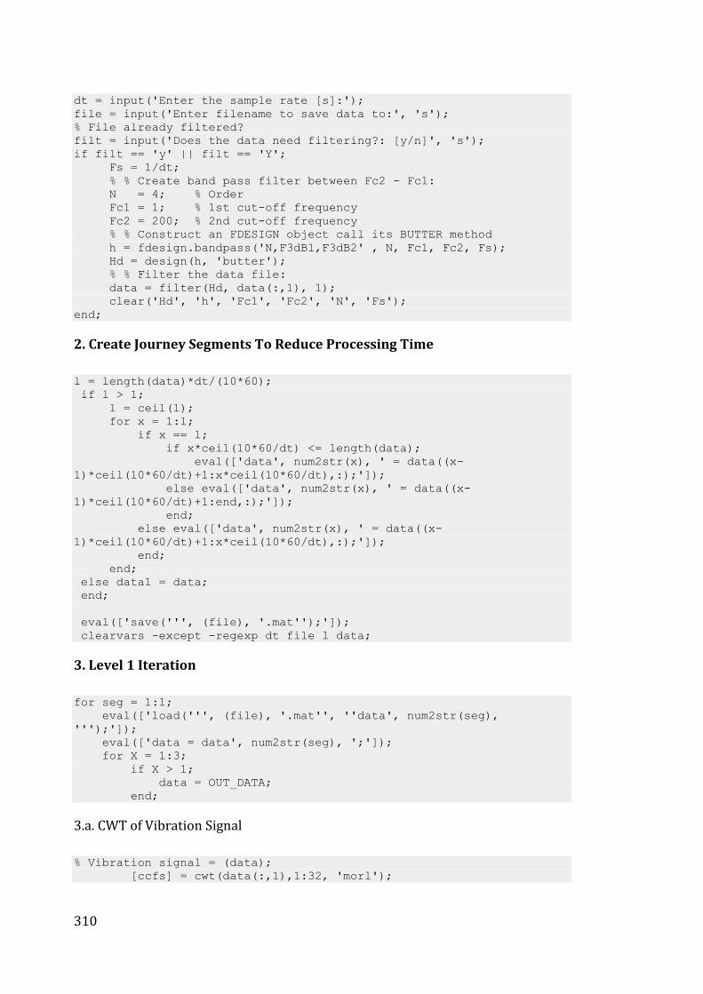
310
dt = input('Enter the sample rate [s]:'); file = input('Enter filename to save data to:', 's'); % File already filtered? filt = input('Does the data need filtering?: [y/n]', 's'); if filt == 'y' || filt == 'Y'; Fs = 1/dt; % % Create band pass filter between Fc2 - Fc1: N = 4; % Order Fc1 = 1; % 1st cut-off frequency Fc2 = 200; % 2nd cut-off frequency % % Construct an FDESIGN object call its BUTTER method h = fdesign.bandpass('N,F3dB1,F3dB2' , N, Fc1, Fc2, Fs); Hd = design(h, 'butter'); % % Filter the data file: data = filter(Hd, data(:,1), 1); clear('Hd', 'h', 'Fc1', 'Fc2', 'N', 'Fs'); end;
2. Create Journey Segments To Reduce Processing Time
l = length(data)*dt/(10*60); if l > 1; l = ceil(l); for x = 1:l; if x == l; if x*ceil(10*60/dt) <= length(data); eval(['data', num2str(x), ' = data((x-1)*ceil(10*60/dt)+1:x*ceil(10*60/dt),:);']); else eval(['data', num2str(x), ' = data((x-1)*ceil(10*60/dt)+1:end,:);']); end; else eval(['data', num2str(x), ' = data((x-1)*ceil(10*60/dt)+1:x*ceil(10*60/dt),:);']); end; end; else data1 = data; end; eval(['save(''', (file), '.mat'');']); clearvars -except -regexp dt file l data;
3. Level 1 Iteration
for seg = 1:l; eval(['load(''', (file), '.mat'', ''data', num2str(seg), ''');']); eval(['data = data', num2str(seg), ';']); for X = 1:3; if X > 1; data = OUT_DATA; end;
3.a. CWT of Vibration Signal
% Vibration signal = (data); [ccfs] = cwt(data(:,1),1:32, 'morl');

311
3.b. Create Gaussian Stationary Signal From PSD
% PSD of signal; lnfft = 2^11; [p,f] = cpsd(data(:,1),data(:,1),[],(lnfft-1),lnfft,(1/dt)); n = round(length(data)*dt); % Find how many seconds needed signal = []; % Vector to store signal for ni = 1:n; a = p(1:end-1,:) .* ((lnfft)/(2*dt)); a = sqrt(a); phase = 2*pi*rand(size(a)); % Random phases in [0 2*pi] Y = a.*exp(j*phase); % Complex vector for ifft % Replicate complex conj Y = [conj(Y(2:end,:));0;flipud((Y(2:end,:)))]; Y = [0;Y]; % Give it zero mean s = (ifft(Y)); % Inverted transform signal = [signal;s]; % Put together = signal end;
3.c. CWT of Simulated Signal
% CWT of simulated signal (signal); [ccfs_G] = cwt(signal,1:32, 'morl');
3.d. Create Gaussian Envelope
% Find the max and min coefficient values in each scale: gmax = max(ccfs_G,[],2); gmin = min(ccfs_G,[],2); clear('-regexp', 'ccfs_G');
3.e. Apply Gaussian Envelope to Vibration Signal
PKLOCS = []; % Find outliers: for i = 1:32; [colm, row] = find(ccfs(i,:) > gmax(i,:) | ccfs(i,:) < gmin(i,:)); PKLOCS = [PKLOCS,row]; end; % Create vector to store all locations exceeding limits of envelope PTS = sort(unique(PKLOCS))'; clear('-regexp', 'PKLOCS'); data = [(1:1:length(data))', (1:1:length(data))', data];
3.f. Remove Outlying Segments from Vibration Signal;
hsize = (2^11)/2; OUT_DATA = []; % Store outlying portions of data i = 1; % For first point set i = 1 while i <= length(PTS)-1; if i > 1; ptx = pt1;

312
end; pt1 = PTS(i,:); pt2 = PTS(i+1,:); % When considering the 1st outlier: if i == 1; % If PTS i : PTS i+1 < hsize points between considered; if pt2-pt1 <= 2*hsize; % if pt1 < hsize, data segment is taken from the start of the signal if pt1 <= hsize; % if pt1 < length(data) – hsize, pt1-hsize : pt1+hsize points removed % If pt1 > length(data) – hsize, pt1-hsize : end are removed; if pt1 <= length(data)-hsize; OUT_DATA = [OUT_DATA; data(1:pt1+hsize,:)]; % All the points greater than pt1 are found; p = find(PTS > pt1); % the new i is calculated as the next point in the series; i = p(1,:); % the old pt1 is stored as ptx for the next iteration; ptx = pt1; else OUT_DATA = [OUT_DATA; data(1:PTS(end,:),:)]; break; % End if length data reached; end; % Where i = 1, pt2-pt1 < hsize and pt1 > hsize; else if pt1 <= length(data)-hsize; OUT_DATA = [OUT_DATA; data((pt1-hsize):pt1+hsize,:)]; p = find(PTS > pt1); if isempty(p) == 0; i = p(1,:); ptx = pt1; else break; end; else OUT_DATA = [OUT_DATA; data(pt1-hsize:PTS(end,:),:)]; break; end; end; % If pt2-pt1 > hsize, skip to next point else i = i+1; end; % When i > 1; else if pt2-pt1 <= 2*hsize; % if pt1 is close to the beginning of the signal (i.e.less than hsize); if pt1 < hsize; % and if pt1 is close to the end; if pt1 <= length(data)- hsize; if pt1 < ptx + 2*hsize; n = (ptx + hsize); else n = pt1 - hsize; end; OUT_DATA = [OUT_DATA; data(n+1:pt1+hsize,:)]; p = find(PTS > pt1); i = p(1,:); ptx = pt1; % When pt1 is less than hsizee from the end signal;

313
else OUT_DATA = [OUT_DATA; data(pt1:PTS(end,:),:)]; i = length(data); break; end; % when pt1 is not close to beginning of signal or close to the end; else if pt1 <= length(data)-hsize; if pt1 < ptx + 2*hsize; n = (ptx + hsize); else n = pt1-hsize; end; OUT_DATA = [OUT_DATA; data((n+1):pt1+hsize,:)]; p = find(PTS > pt1); if isempty(p) == 0; i = p(1,:); ptx = pt1; else break; end; % If close to end take end of signal and break; else if pt1 < ptx + 2*hsize; n = (ptx + hsize); else n = pt1-hsize; end; OUT_DATA = [OUT_DATA; data(n+1:PTS(end,:),:)]; i = length(data); break; end; end; else i = i+1; end; end; end; % Put gen_vib segments that are less than half a second back into the % out_data (sample size deemed too small); dif = diff(OUT_DATA(:,1)); ptz = find(dif > 1 & dif < 2*hsize); if isempty(ptz) ~= 1; ptz = [ptz; data(end,1)]; for z = 1:length(ptz); if z < length(ptz); p1 = OUT_DATA(ptz(z,:),1)+1; p2 = OUT_DATA((ptz(z,:)+1),1)-1; OUT_DATA = [OUT_DATA; data(p1:p2,:)]; else p1 = OUT_DATA(ptz(z-1,:)+1,1)+1; p2 = data((ptz(z,:)),1); if p2-p1 < 2*hsize; OUT_DATA = [OUT_DATA; data(p1:p2,:)]; end; end; end; end; OUT_DATA = sortrows(OUT_DATA,1); % Find low level vibration = Gaussian Approximation:

314
eval([(file), '_L1_', num2str(X), ' = data;']); eval([(file), '_L1_', num2str(X), ' (OUT_DATA(:,1),:) = [];']); if data < ceil(1/dt); OUT_DATA = [OUT_DATA; data]; OUT_DATA = sortrows(OUT_DATA,1); eval([(file), '_L1_', num2str(X), ' = [];']); end; data = OUT_DATA; OUT_DATA = OUT_DATA(:,3); eval(['',(file), '_L1_', num2str(X), ' = ', (file), '_L1_', num2str(X), '(:,3);']); eval(['save(''', (file), '.mat'', ''-regexp'', ''', (file), '_L'', ''-append'');']); clear('-regexp', 'ccfs_', '_L1'); end; % Save data files and save last non-Gaussian (OUT_DATA) as the l+1 Gaussian approximation and renumber data parts so that non are repeated: eval(['', (file), '_L1_', num2str(X+1), ' = OUT_DATA;']); eval(['save(''', (file), '.mat'', ''-regexp'', ''', (file), '_L'', ''-append'');']); no = X+1; eval(['load(''', (file), '.mat'', ''-regexp'', ''', (file), '_L1_'');']); for X = 1:4; eval(['', (file), '_L1s_', num2str(((no)*(seg-1))+X), ' = ', (file), '_L1_', num2str(X), ';']); end; eval(['save(''', (file), '.mat'', ''-append'', ''-regexp'', ''', (file), '_L1_'');']); clear -regexp _L1_ data OUT_DATA signal; end; % TOTAL Number of segments: seg = seg*(X);
4. Level 2 Iteration
% I is the number of iterations of each of the data samples carried out. % Maximum number of segments per data sample = I+1; iter = 0; for X = 1:seg; iter = iter+1 for I = 1:4; if I == 1; eval(['load(''', (file), '.mat'', ''', (file), '_L1s_', num2str(X), ''');']); eval(['data = ', (file), '_L1s_', num2str(X), '(:,1);']); if isempty(data) == 1; break; else data = data; end; eval(['clear(''', (file), '_L1s_', num2str(X), ''');']); else

315
eval(['load(''', (file), '.mat'', ''', (file), '_L2_', num2str(X), '_', num2str(I-1), ''');']); eval(['length_predata = length(', (file), '_L2_', num2str(X), '_', num2str(I-1), ');']); eval(['clear(''', (file), '_L2_', num2str(X), '_', num2str(I-1), ''');']); eval(['data = OUT_DATA(:,3);']); if length(data) == length_predata; break; end; end;
4.a. CWT of Vibration Signal
% Vibration signal = Gaussian approximation from 1st iteration = (data); [ccfs] = cwt(data(:,1),1:32, 'morl'); eval(['save(''', (file), '.mat'', ''-append'', ''ccfs'');']); clear -regexp ccfs;
4.b. Create Gaussian Stationary Signal From PSD
% PSD of signal; lnfft = 2^11; [p,f] = cpsd(data(:,1),data(:,1),[],(lnfft-1),lnfft,(1/dt)); n = round(length(data)/lnfft); % Find how many seconds needed signal = []; for ni = 1:n; a = p .* ((lnfft)/(2*dt)); a = sqrt(a); phase = 2*pi*rand(size(a)); % Random phases in [0 2*pi] Y = a.*exp(j*phase); % Complex vector for ifft Y = [Y;flipud(conj(Y))]; % Replicate complex conj Y = [0;Y]; % Give it zero mean s = ifft(Y); % Invertedtransform signal = [signal;s]; % Put together to create signal end;
4.c. CWT of Simulated Signal
% CWT of simulated signal (signal); [ccfs_G] = cwt(signal,1:32, 'morl'); % Find the max and min coefficient values in each scale: eval(['gmax = max(ccfs_G,[],2);']); eval(['gmin = min(ccfs_G,[],2);']);
4.d. Create Gaussian Envelope
% Find the max and min coefficient values in each scale: clear -regexp ccfs eval(['load(''', (file), '.mat'', ''ccfs'');']);
4.e. Apply Gaussian Envelope to Vibration Signal

316
PKLOCS = []; % Find outliers: for i = 1:32; [colm, row] = find(ccfs(i,:) > gmax(i,:) | ccfs(i,:) < gmin(i,:)); PKLOCS = [PKLOCS,row]; end; PTS = sort(unique(PKLOCS))'; ccfs = []; eval(['save(''', (file), '.mat'', ''-append'', ''ccfs'');']); clear -regexp ccfs signal; data = [(1:1:length(data))', (1:1:length(data))', data];
4.f. Remove Outlying Segments from Vibration Signal;
hsize = (2^11)/2; OUT_DATA = []; % Store outlying portions of data % For first point set i = 1: i = 1; while i <= length(PTS)-1; if i > 1; ptx = pt1; end; pt1 = PTS(i,:); pt2 = PTS(i+1,:); % When considering the 1st outlier; if i == 1; % If PTS i : PTS i+1 < hsize all points between considered; if pt2-pt1 <= 2*hsize; % if the pt1 < hsize, data segment from start of the signal; if pt1 <= hsize; % if pt1 < length(data) – hsize, pt1-hsize : pt1+hsize removed; If pt1 > length(data) – hsize, pt1-hsize : end are removed; if pt1 <= length(data)-hsize; OUT_DATA = [OUT_DATA; data(1:pt1+hsize,:)]; % All the points greater than pt1 are found; p = find(PTS > pt1); % the new i is calculated as the next point in the series; i = p(1,:); % the old pt1 is stored as ptx for the next iteration; ptx = pt1; else OUT_DATA = [OUT_DATA; data(1:PTS(end,:),:)]; break; % length(data) reached end; end; % Where i = 1, pt2-pt1 < hsize and pt1 > hsize; else if pt1 <= length(data)-hsize; OUT_DATA = [OUT_DATA; data((pt1-hsize):pt1+hsize,:)]; p = find(PTS > pt1); if isempty(p) == 0; i = p(1,:); ptx = pt1; else break; end; else OUT_DATA = [OUT_DATA; data(pt1-hsize:PTS(end,:),:)];

317
break; end; end; % If pt2-pt1 > hsize, skip to next point; else i = i+1; end; % If i > 1 else if pt2-pt1 <= 2*hsize; % if pt1 and pt2 are close; % if pt1 is close to the beginning of the signal; if pt1 < hsize; % and if pt1 is close to the end; if pt1 <= length(data)- hsize; if pt1 < ptx + 2*hsize; n = (ptx + hsize); else n = pt1 - hsize; end; OUT_DATA = [OUT_DATA; data(n+1:pt1+hsize,:)]; p = find(PTS > pt1); i = p(1,:); ptx = pt1; % When pt1 < length(signal) –hsize, take the data to the end; else OUT_DATA = [OUT_DATA; data(pt1:PTS(end,:),:)]; i = length(data); break; end; % when pt1 is not close to beginning of signal or close to end; else if pt1 <= length(data)-hsize; if pt1 < ptx + 2*hsize; n = (ptx + hsize); else n = pt1-hsize; end; OUT_DATA = [OUT_DATA; data((n+1):pt1+hsize,:)]; p = find(PTS > pt1); if isempty(p) == 0; i = p(1,:); ptx = pt1; else break; end; % If close to end take to the end of signal and break; else if pt1 < ptx + 2*hsize; n = (ptx + hsize); else n = pt1-hsize; end; OUT_DATA = [OUT_DATA; data(n+1:PTS(end,:),:)]; i = length(data); break; end; end; else i = i+1; end; end; end; % Put segments from Gaussian approximation (low level vibration) less than half a second back in out_data; if isempty(OUT_DATA) == 0;

318
dif = diff(OUT_DATA(:,1)); ptz = find(dif > 1 & dif < 2*hsize+1); if isempty(ptz) == 0; ptz = [ptz; data(end,1)]; for z = 1:length(ptz); if z < length(ptz); p1 = OUT_DATA(ptz(z,:),1)+1; p2 = OUT_DATA((ptz(z,:)+1),1)-1; OUT_DATA = [OUT_DATA; data(p1:p2,:)]; else p1 = OUT_DATA(ptz(z-1,:)+1,1)+1; p2 = data((ptz(z,:)),1); if p2-p1 < 2*hsize+1; OUT_DATA = [OUT_DATA; data(p1:p2,:)]; end; end; end; else ptz = []; end; OUT_DATA = sortrows(OUT_DATA,1); OUT_DATA = unique(OUT_DATA, 'rows'); end; % Find and plot the Gaussian Approximation vibration; eval([(file), '_L2_', num2str(X), '_', num2str(I), ' = data;']); if isempty(OUT_DATA) == 0; OUT_DATA = unique(OUT_DATA, 'rows'); eval([(file), '_L2_', num2str(X), '_', num2str(I), ' (OUT_DATA(:,1),:) = [];']); eval(['len = length(', (file), '_L2_', num2str(X), '_', num2str(I), ');']); end; if len < lnfft; % < ceil(1/dt); OUT_DATA = [OUT_DATA; data]; OUT_DATA = sortrows(OUT_DATA,1); OUT_DATA = unique(OUT_DATA,'rows'); eval([(file), '_L2_', num2str(X), '_', num2str(I), ' = [];']); end; data = OUT_DATA; % Save data as Gaussian approximations, if length > 0; eval(['l = length(', (file), '_L2_', num2str(X), '_', num2str(I), ');']); if l > 0; eval(['', (file), '_L2_', num2str(X), '_', num2str(I), '= ', (file), '_L2_', num2str(X), '_', num2str(I), '(:,3);']); end; eval(['save(''', (file), '.mat'', ''-regexp'', ''', (file), '_L2_'', ''-append'');']); end; % Save all segments and save final OUT_DATA as the X + 1 data file; eval(['', (file), '_L2_', num2str(X), '_', num2str(I+1), ' = OUT_DATA;']); eval(['save(''', (file), '.mat'', ''-regexp'', ''', (file), '_L2_'', ''-append'');']); clear -regexp OUT_DATA; eval(['clear(''-regexp'', ''ccfs_'', ''', (file), '_L2'');']); clear -regexp PKLOCS; eval(['', (file), '_L1s_', num2str(X), ' = [];']);

319
eval(['save(''', (file), '.mat'', ''-append'', ''', (file), '_', num2str(X), ''');']); end;
6. Create the Simulation
x = 1; PSD = []; RMS = []; KURTOSIS = []; DURATION = []; for X = 1:seg; for I = 1:5; eval(['load(''', (file), '.mat'', ''', (file), '_L2_', num2str(X), '_', num2str(I), ''');']); eval(['data = ', (file), '_L2_', num2str(X), '_', num2str(I), ';']); if isempty(data) == 0; if size(data,2) > 1; data = data(:,3); end; eval(['clear(''-regexp'', ''', (file), '_L2_'');']);
6.a. For Each Part Calculate PSD
lnfft = 2^11; if length(data) > 2050; olap = 2^11-1; else olap = 0; end; [p,f] = cpsd(data,data,[],olap,lnfft,(1/dt)); PSD = [PSD, [x;p]];
6.b. Evaluate Segment Statistics
rms = norm(data) / sqrt(length(data)); RMS = [RMS; x, rms]; k = kurtosis(data); KURTOSIS = [KURTOSIS; x, k]; duration = length(data) * dt; DURATION = [DURATION; x, duration];
6.c. For Each Part Calculate a Gaussian Stationary Signal From PSD
% Inverted PSD to create signal; n = round(length(data)*dt); % Find how many seconds needed n = round(n*(1/dt)/lnfft); eval(['signal_', num2str(x), ' = [];']); for ni = 1:n; a = p(1:end-1,:) .* ((lnfft)/(2*dt)); a = sqrt(a); phase = 2*pi*rand(size(a)); % Random phases in [0 2*pi]

320
Y = a.*exp(j*phase); % Complex vector for ifft % Replicate complex conj Y = [conj(Y(2:end,:));0;flipud((Y(2:end,:)))]; Y = [0;Y]; % Give it zero mean s = (ifft(Y)); % Inverted transform % Put together to create signal for each Gaussian approximation part; eval(['signal_', num2str(x), ' = [signal_', num2str(x), ';s];']); end; eval(['save(''', (file), '.mat'', ''-append'', ''signal_', num2str(x), ''');']); x = x+1; end; end; end; x = x-1; % Save files; eval(['save(''', (file), '.mat'', ''-append'', ''x'', ''RMS'', ''KURTOSIS'', ''DURATION'', ''f'', ''PSD'');']); clearvars -except -regexp PSD x f dt lnfft signal file; % Create spline for simplified PSD for each segment; xx = [1:1:5, 7, 10, 12, 15, 17, 20:5:50, 60, 80, 100, 150, 200, 250]; figure(100); hold on; col = lines(x); for i = 1:x; eval(['yy', num2str(i), ' = spline(f, PSD(2:end, i), xx);']); eval(['loglog(xx, yy', num2str(i), ', ''color'', col(i,:));']); end; eval(['save(''', (file), '.mat'', ''-append'', ''-regexp'', ''yy'', ''xx'');']);
6.d. Randomise Order of Parts to Create Simulation Signal
% signal = simulation signal; % dt = simulation signal dt; Nofiles = x; nf = randperm(Nofiles); signal = []; for i = 1:Nofiles; eval(['load(''', (file), '.mat'', ''signal_', num2str(nf(:,i)), ''');']); eval(['signal = [signal; signal_', num2str(nf(:,i)), '];']); end; % Plot simulation signal; figure(65); plot((0:(1/dt):(length(signal)-1)*(1/dt))', signal); eval(['save(''', (file), '.mat'', ''signal'', ''-append'');']);
Published with MATLAB® 7.11