An Improved Frequent

Pattern Mining Algorithm

Using Suffix Tree & Suffix

Automata

MD. SABBIR AHMED Reg. No. : 10101020

MOHAMMAD RIAJUR RAHMAN Reg. No. : 10101006

MD. MOTAHER HOSSAIN Reg. No. : 10101024

MD. KHALID HASAN Reg. No. : 10101025

Submitted in partial fulfillment of the degree of

Bachelor of Science, with Honours at University of Asia Pacific, Dhaka,

Bangladesh.

29 May, 2014

DECLARATION

We, hereby, declare that the work presented in this thesis is the outcome of the

investigation performed by us under the supervision of Md. Shiplu Hawlader, Lecturer,

Department of Computer Science and Engineering, University of Asia Pacific. We also

declare that no part of this thesis and thereof has been or is being submitted elsewhere

for the award of any degree or diploma.

Signature Signature

MD. SABBIR AHMED

Candidate

MOHAMMAD RIAJUR RAHMAN

Candidate

Countersigned

Md. Shiplu Hawlader

Supervisor

Signature Signature

MD. MOTAHER HOSSAIN

Candidate

MD. KHALID HASAN

Candidate

APPROVAL

The Thesis Report " An Improved Frequent Pattern Mining Algorithm Using Suffix Tree

& Suffix Automata" submitted by MD. SABBIR AHMED, Reg.NO.10101020;

MOHAMMAD RIAJUR RAHMAN, Reg.NO.10101006; MD. MOTAHER HOSSAIN,

Reg.NO.:10101024, MD.KHALID HASAN, Reg.NO.:10101025 students of Spring-2010,

to the Department of Computer Science & Engineering, University of Asia Pacific, has

been accepted as satisfactory for the partial fulfillment of the requirements for the

degree of Bachelor of Science in Computer Science & Engineering and approved as to

its style and contents.

Approved as to the style & contents by

Md. Firoz Mridha

Assistant Professor

Department of Computer Science & Engineering,

University of Asia Pacific

Dr. Md. Shahriar Rahman

Assistant Professor

Department of Computer Science & Engineering,

University of Asia Pacific

Md. Akhtaruzaman Adnan

Lecturer

Department of Computer Science & Engineering,

University of Asia Pacific

ACKNOWLEDGEMENTS

First of all, thanks to Almighty Allah for giving us the potency and energy to complete

this thesis successfully.

We want to express out gratefulness towards our thesis supervisor Md. Shiplu Hawlader

for his valuable advices and important suggestions. His regular and active supervision

and erudite directions from the beginning to the end were the driving forces for the

successful completion of the research work.

We would like to convey our thankfulness to all of our teachers at the Department of

Computer Science and Engineering, University of Asia Pacific. Discussions with many

of them have helped us tremendously in improving the quality of our work. We also

thank the department for providing us with resources which were necessary for the

preparation of the thesis. And last but not the least, we would like to express thanks to our parents and family

members for their tremendous support and inspiration.

ABSTRACT

As with the advancement of the IT technologies, the amount of accumulated data is also

increasing. It has resulted in large amount of data stored in databases, warehouses and

other repositories. Thus the Data mining comes into picture to explore and analyze the

databases to extract the interesting and previously unknown patterns and rules known

as association rule mining. Association Rule Mining is used to Finding frequent patterns,

associations, correlations, or causal structures among sets of items or objects in

transaction databases, relational databases, and other information repositories. Many

algorithms have been proposed from last many decades for solving frequent pattern

mining. Among different approaches to solve frequent pattern mining, a relatively new

one is an improved frequent pattern mining algorithm using suffix tree & suffix automata.

Previous researches we found which were based on prefix tree. In this paper, we have

proposed a new frequent pattern mining algorithm which based on suffix tree & suffix

automata. Experimental results on synthetic datasets show that the proposed algorithm

provides better accuracy compared to previous algorithms.

Contents

1 Introduction 1

1.1 Motivation ……………………………………………………………………… 3

1.2 Aims & Objectives ……………………………………………………………. 4

1.3 Outlines of This Thesis ………………………………………………………. 4

2 Data Mining 5

2.1 Basic Concept ……………………………………………………………………… 5

2.2 Data Mining Applications …………………………………………………….. 6

2.3 The Primary Methods of Data Mining ………………………………………. 8

3 Basic Concepts of Association Rule Mining 9

3.1 Definition ………………………………………………………………………. 10

3.2 Rule Evaluation Metrics ……………………………………………………… 10

3.3 Basic Concepts ……………………………………………………………….. 11

3.4 Observations ………………………………………………………………….. 12

3.5 Association Model ……………………………………………………………. 12

3.6 Problem of Association Rules ………………………………………………. 12

4 Literature Review 13

4.1 The Apriori Algorithm .…….. ………………………………………………... 13

4.1.1 The Apriori Algorithm in a Nutshell …………………………………. 14

4.1.2 The Apriori Algorithm: Pseudo code………………………………… 15

4.1.3 Setting ……………………………………………………….…………. 15

4.1.4 Limitations ……………………………………………………………... 16

4.1.5 The Apriori Algorithm: Example ……………………………….…….. 17

4.1.6 Methods to Improve Apriori’s Efficiency ………………………….... 22

4.1.7 Principle ……………………………………………………………….. 23

4.1.8 Flow chart of Apriori Algorithm …..…………………………..……… 24

4.1.9 Hash based method of Apriori Algorithm ………………..…………. 24

4.1.10 Graph based approach ……………………………………………... 25

4.1.11 Performance …………………………………………………………. 25

4.1.12 Problem ………………………………………………………………. 26

4.1.13 Discussion …………………………………………………………… 26

4.2 FP-Growth Algorithm ………………………………………………………… 27

4.2.1 Preprocessing …….…………………………………………………… 28

4.2.2 Applications ….…………………….………………………………….. 29

4.2.3 FP-Growth Method: Construction of FP-Tree …………………….... 30

4.2.4 Mining the FP-Tree by Creating Conditional (sub) pattern bases .. 30

4.2.5 FP-Growth Method: An Example…………………………………….. 31

4.2.6 Advantages of FP-Growth ………………………………..………….. 33

4.2.7 Disadvantages of FP-Growth ……………………………...………… 33

4.2.8 Why Frequent Pattern Growth Fast ……………………..………….. 33

4.3 Prefix Tree……………………………………………………………………… 34

4.4 Suffix Tree……………………………………………………………………… 34

4.4.1 Definition……………………………………………………………….. 35

4.4.2 Applications……………………………………………………………. 36

4.4.3 Functionality…………………………………………………………… 36

4.5 Related Work………………………………………………………………….. 38

5 The Proposed Algorithm 39

5.1 Suffix Tree …………………………………………………………………….. 39

5.2 Ukkonen's algorithm………………………………………………………….. 40

5.3 Suffix automata……………………………………………………………….. 40

5.4 Algorithm………………………………………………………………………. 41

5.5 Procedure……………………………………………………………………… 41

6 Performances Analysis 46

6.1 Complexity Analysis………………………………………………………….. 46

6.2 Environments of Experiments………………………………………………. 46

7 Conclusion 50

7.1 Future Trends…………………………………………………………………. 51

References 52

List of Tables

1-1 Example of Frequent Pattern………………………………………………….. 3

3-1 Definition of Association Rule…………………………………………………. 10

3-2 Example of Support & Confidence……………………………………………. 11

4-1 Apriori Example…………………………………………………………………. 17

4-2 FP-Growth Example……………………………………………………………. 31

4-3 Mining the FP-Tree by creating conditional (sub) pattern bases………….. 32

6-1 Complexity Analysis……………………………………………………………. 46

List of Figures

2-1 Data mining is the core of Knowledge discovery process………………….. 6

2-2 Data mining applications in2008……………………………………………… 7

4-1 First step of Apriori Algorithm…………..……………………………………… 18

4-2 Second step of Apriori Algorithm ……………………………………………... 19

4-3 Third step of Apriori Algorithm…...……………………………………………. 20

4-4 Principle of Apriori Algorithm …………………………………………………. 23

4-5 Flow chart of Apriori Algorithm.……………………………………………….. 24

4-6 Transaction database (left), item frequencies (middle), and reduced

transaction database with items in transactions sorted descending

W.R.T. their frequency (right)…………………………………………………..

29

4-7 An FP-Tree that registers compressed, frequent pattern information…….. 32

5-1 Example of Suffix Tree…………………………………………………………. 39

5-2 Figure 5-2: (a) A deterministic finite automation A and (b) a deterministic

automation recognizing ∑*L(A) where transitions labeled with φ are

failure transitions………………………………………………………………...

40

5-3 Contraction of Build Tree………………………………………………………. 43

5-4 Frequent Pattern is B(2)……………………………………………………….. 44

5-5 Frequent Pattern is A(2)……………………………………………………….. 44

5-6 Frequent Pattern is D(3), DA(2), DB(2)………………………………………. 44

5-7 Frequent Pattern is C(3), CD(3), CB(2), CA(2), CDA(2)……………………. 45

6-1 Comparison between Apriori, FP-Growth, CP-Tree & Proposed Algorithm

on T10I4D100K Data……………………………………………………………

48

6-2 Comparison between Apriori, FP-Growth, CP-Tree & Proposed Algorithm

on Mushroom Data Set…………………………………………………………

49

Chapter 1

Introduction

Data mining has enticed a great deal of attention in the information industry and in

society as a whole in recent years, due to the extensive availability of huge amounts of

data and the ensuing need for turning such data into useful information and knowledge.

The information and knowledge gained can be used for applications ranging from

market analysis, fraud detection, and customer retention, to production control and

science exploration.

Data mining offers to extracting or “mining” knowledge from large amounts of data. The

term is actually a misnomer. Remember that the mining of gold from rocks or sand is

referred to as gold mining rather than rock or sand mining. Thus, data mining should

have been more appropriately named “knowledge mining from data,” which is

unfortunately somewhat long. “Knowledge mining,” a shorter term may not reflect the

emphasis on mining from large amounts of data. Nevertheless, mining is a sprightly

term characterizing the process that finds a small set of precious nuggets from a great

deal of raw material. Thus, such a misnomer that carries both “data” and “mining”

became a popular choice. Many other terms carry a similar or slightly different meaning

to data mining, such as knowledge mining from data, knowledge extraction, data/pattern

analysis, data archaeology, and data dredging. Many people treat data mining as a

synonym for another popularly used term, Knowledge Discovery from Data, or KDD.

KDD applications deliver measurable benefits, including reduced cost of doing

business, enhanced profitability, and improved quality of service. Therefore Knowledge

Discovery in Databases has become one of the most active and exciting research areas

in the database community.

Cluster analysis or clustering is the task of grouping a set of objects in such a way that

objects in the same group (called a cluster) are more similar (in some sense or another)

to each other than to those in other groups (clusters). It is a main task of empiric data

mining, and a common technique for statistical data analysis, used in many fields,

including machine learning, pattern recognition, image analysis, information retrieval,

and bioinformatics.

Cluster analysis itself is not one specific algorithm, but the general task to be solved. It

can be achieved by various algorithms that differ significantly in their notion of what

constitutes a cluster and how to efficiently find them. Popular notions of clusters include

groups with small distances among the cluster members, dense areas of the data

space, intervals or particular statistical distributions. Clustering can therefore be

formulated as a multi-objective optimization problem. The appropriate clustering

algorithm and parameter settings depend on the individual data set and intended use of

the results. Cluster analysis as such is not an automatic task, but an iterative process

of knowledge discovery or interactive multiple objective optimization that involves trial

and failure. It will often be necessary to modify data reprocessing and model

parameters until the result achieves the desired properties. So, the goal of clustering is

to determine the intrinsic grouping in a set of unlabeled data. [2]

Frequent pattern mining has been a focused theme in data mining research for over a

decade. Abundant literature has been dedicated to this research and tremendous

progress has been made, ranging from efficient and scalable algorithms for frequent

item-set mining in transaction databases to numerous research frontiers, such as

sequential pattern mining, structured pattern mining, correlation mining, associative

classification, and frequent pattern-based clustering, as well as their broad applications.

Frequent pattern mining was first proposed by Agrawal et al. (1993) for market basket

analysis in the form of association rule mining. It analyses customer buying habits by

finding associations between the different items that customers place in their “shopping

baskets”. For instance, if customers are buying milk, how likely are they going to also

buy cereal (and what kind of cereal) on the same trip to the supermarket? Such

information can lead to increased sales by helping retailers do selective marketing and

arrange their shelf space. [3]

Frequent pattern is an intrinsic and important property of data-sets. Foundation for

many essential data mining tasks, some are given below:

Association, correlation, and causality analysis.

Sequential, structural (e.g., sub-graph) patterns.

Pattern analysis in spatiotemporal, multimedia, time series, and stream data.

Classification: discriminative, frequent pattern analysis.

Cluster analysis: frequent pattern-based clustering.

Data warehousing: iceberg cube and cube-gradient.

Semantic data compression: fascicles.

Broad applications.

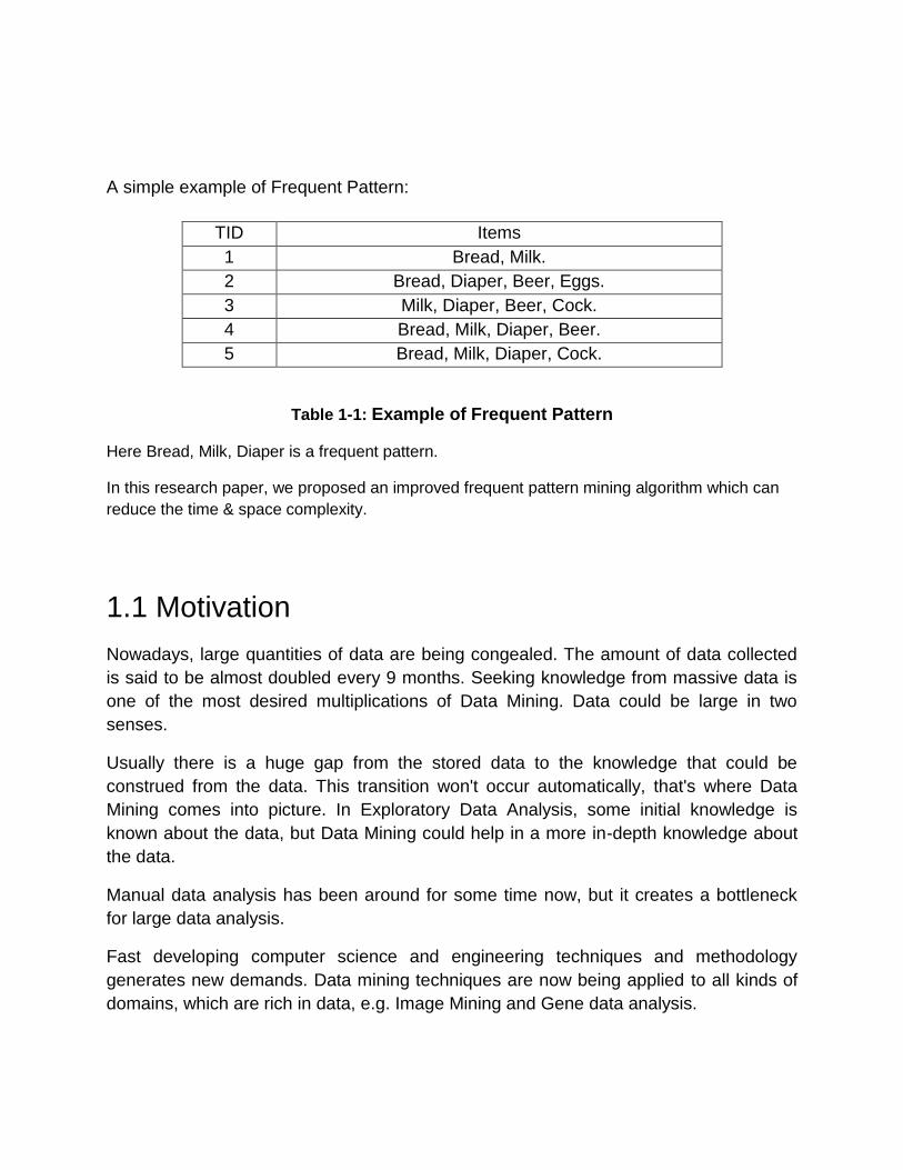
A simple example of Frequent Pattern:

TID Items

1 Bread, Milk.

2 Bread, Diaper, Beer, Eggs.

3 Milk, Diaper, Beer, Cock.

4 Bread, Milk, Diaper, Beer.

5 Bread, Milk, Diaper, Cock.

Table 1-1: Example of Frequent Pattern

Here Bread, Milk, Diaper is a frequent pattern.

In this research paper, we proposed an improved frequent pattern mining algorithm which can

reduce the time & space complexity.

1.1 Motivation

Nowadays, large quantities of data are being congealed. The amount of data collected

is said to be almost doubled every 9 months. Seeking knowledge from massive data is

one of the most desired multiplications of Data Mining. Data could be large in two

senses.

Usually there is a huge gap from the stored data to the knowledge that could be

construed from the data. This transition won't occur automatically, that's where Data

Mining comes into picture. In Exploratory Data Analysis, some initial knowledge is

known about the data, but Data Mining could help in a more in-depth knowledge about

the data.

Manual data analysis has been around for some time now, but it creates a bottleneck

for large data analysis.

Fast developing computer science and engineering techniques and methodology

generates new demands. Data mining techniques are now being applied to all kinds of

domains, which are rich in data, e.g. Image Mining and Gene data analysis.

Data mining also face some challenges: Increasing data dimensionality and data size,

various forms of data, new types of data like streaming data and multimedia data,

Efficiency in data access and Information search methods, intelligent upgrade and

integration methods. [4]

1.2 Aims & Objectives

Many frequent pattern mining algorithm exist for generating frequent pattern itemsets.

After studying these algorithms we found that these algorithms have a limitation which is

scanning the database in multiple times. So, it took more space & time for generating

frequent pattern itemsets. Our aim is to develop a new algorithm which will scan the

database at beginning time. As a result it reduces time & space complexity. For

implementing our algorithm we use suffix tree (ukkonen’s) which reduces the time

complexity and for reducing space complexity we use suffix automata.

Our main objective is to develop some algorithm like apriori, fp-tree, ukkonen’s which

results the frequent pattern mining itemsets. Then compare these previous implemented

algorithms with our proposed algorithm.

1.3 Outline of the Thesis

The rest of the chapters are organized as follows. Chapter 2 presents Basic Concepts

of Data Mining and its applications. In Chapter 3, Basic Concepts of Association Rule

Mining. In Chapter 4, Literature Review with Apriori Algorithm, FP-Growth Algorithm &

basic concepts about Proposed Algorithm. In Chapter 5, The Proposed Algorithm has

been described clearly. In Chapter 6 contains the Performance Analysis. Finally,

Chapter 7 contains Conclusion & the Future Work of the new Algorithm.

Chapter 2

Data Mining

With the increase in Information Technology, the size of the databases created by the

organizations due to the availability of low-cost storage and the evolution in the data

capturing technologies is also increasing. These organization sectors include retail,

petroleum, telecommunications, utilities, manufacturing, transportation, credit cards,

insurance, banking and many others, extracting the valuable data, it necessary to

explore the databases completely and efficiently. Knowledge discovery in databases

(KDD) helps to identifying precious information in such huge databases. This valuable

information can help the decision maker to make accurate future decisions.

2.1 Basic Concept

This is the important part of KDD. Data mining generally involves four classes of task;

classification, clustering, regression, and association rule learning. Data mining refers to

discover knowledge in huge amounts of data. It is a scientific discipline that is

concerned with analyzing observational data sets with the objective of finding

unsuspected relationships and produces a summary of the data in novel ways that the

owner can understand and use. Data mining as a field of study involves the merging of

ideas from many domains rather than a pure discipline the four main disciplines [15],

which are contributing to data mining include:

Statistics: it can provide tools for measuring significance of the given data,

estimating probabilities and many other tasks (e. g. linear regression).

Machine learning: it provides algorithms for inducing knowledge from given data

(e. g. SVM).

Data management and databases: since data mining deals with huge size of

data, an efficient way of accessing and maintaining data is necessary.

Artificial intelligence: it contributes to tasks involving knowledge encoding or

search techniques (e. g. neural networks).

Figure 2-1: Data mining is the core of Knowledge discovery process. [16]

2.2 Data Mining Applications

Data mining has become an essential technology for businesses and researchers in

many fields, the number and variety of applications has been growing gradually for

several years and it is predicted that it will carry on to grow. A number of the

business areas with an early embracing of DM into their processes are banking,

insurance, retail and telecom. More lately it has been implemented in

pharmaceutics, health, government and all sorts of e-businesses.

Figure 2-2: Data mining applications in2008 [17].

One describes a scheme to generate a whole set of trading strategies that take into

account application constraints, for example timing, current position and pricing [18].

The authors highlight the importance of developing a suitable back testing

environment that enables the gathering of sufficient evidence to convince the end

users that the system can be used in practice. They use an evolutionary

computation approach that favors trading models with higher stability, which is

essential for success in this application domain.

Apriori algorithm is used as a recommendation engine in an E-commerce system.

Based on each visitor‘s purchase history the system recommends related, potentially

interesting, products. It is also used as basis for a CRM system as it allows the

company itself to follow-up on customer‘s purchases and to recommend other

products by e-mail[19].

A government application is proposed by [20]. The problem is connected to the

management of the risk associated with social security clients in Australia. The

problem is confirmed as a sequence mining task. The action ability of the model

obtained is an essential concern of the authors. They concentrate on the difficult

issue of performing an evaluation taking both technical and business interestingness

into account.

2.3 The Primary Methods of Data Mining

Data mining addresses two basic tasks: verification and discovery. The verification

task seeks to verify user’s hypotheses. While the discovery task searches for

unknown knowledge hidden in the data. In general, discovery task can be further

divided into two categories, which are descriptive data mining and predicative data

mining.

Descriptive data mining describes the data set in a summery manner and presents

interesting general properties of the data. Predictive data mining constructs one or

more models to be later used for predicting the behavior, of future data sets.

There are a number of algorithmic techniques available for each data mining tasks,

with features that must be weighed against data characteristics and additional

business requirements. Among all the techniques, in this research, we are focusing

on the association rules mining technique, which is descriptive mining technique,

with transactional database system. This technique was formulated by [21] and is

often referred to as market-basket problem.

Chapter 3

Basic Concepts of Association Rule

Mining

Association rules are one of the major techniques of data mining. Association rule

mining finding frequent patterns, associations, correlations, or causal structures among

sets of items or objects in transaction databases, relational databases, and other

information repositories [13]. The volume of data is increasing dramatically as the data

generated by day-to-day activities. Therefore, mining association rules from massive

amount of data in the database is interested for many industries which can help in many

business decision making processes, such as cross-marketing, Basket data analysis,

and promotion assortment. The techniques for discovering association rules from the

data have traditionally focused on identifying relationships between items telling some

aspect of human behaviour, usually buying behaviour for determining items that

customers buy together. All rules of this type describe a particular local pattern. The

group of association rules can be easily interpreted and communicated.

Association Rule was first proposed by Agrawal et al in 1993. It is an important data

mining model studied extensively by the database and data mining community. It

assumes all data are categorical. It has no good algorithm for numeric data. Initially

used for Market Basket Analysis to find how items purchased by customers are related.

Many studies have been conducted to address various conceptual, implementation, and

application issues relating to the association rules mining task. Researcher in

application issues focuses on applying association rules to a variety of application

domains. For example: Relational Databases, Data Warehouses, Transactional

Databases, and Advanced Database Systems (Object-Relational, Spatial and

Temporal, Time-Series, Multimedia, Text, Heterogeneous, Legacy, Distributed, and

WWW) [22].

3.1 Definition

Let us consider an item-set, as like below:

TID Items

1 Bread, Milk.

2 Bread, Diaper, Beer, Eggs.

3 Milk, Diaper, Beer, Cock.

4 Bread, Milk, Diaper, Beer.

5 Bread, Milk, Diaper, Cock.

Table 3-1: Definition of Association Rule

An implication expression of the form X →Y, where X and Y are item-sets

Example: {Milk, Diaper} → {Beer}.

3.2 Rule Evaluation Metrics

Support (s)

Fraction of transactions that contain both X and Y. Which is expressed:

(Day) = P(X U Y)

Confidence (c)

Measures how often items in Y appear in transactions that contain X.

Which is expressed: Day = P (Y|X) = P(X U Y) / P (X).

Suppose computer & Game CD a Movie DVD with minimum confidence and support

Support, s, probability that a transaction contains {Computer, Game CD,

Movie DVD}

Confidence, c, conditional probability that a transaction having {Computer,

Game CD} also contains Movie DVD.

Example:

Transaction ID Items Bought

2000 A,B,C

1000 A,C

4000 A,D

5000 B,E,F

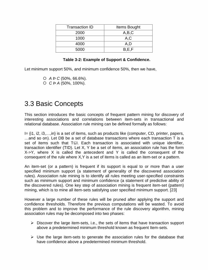
Table 3-2: Example of Support & Confidence.

Let minimum support 50%, and minimum confidence 50%, then we have,

A Þ C (50%, 66.6%). C Þ A (50%, 100%).

3.3 Basic Concepts This section introduces the basic concepts of frequent pattern mining for discovery of interesting associations and correlations between item-sets in transactional and relational database. Association rule mining can be defined formally as follows: I= {i1, i2, i3,…,in} is a set of items, such as products like (computer, CD, printer, papers, …and so on). Let DB be a set of database transactions where each transaction T is a

set of items such that T⊆I. Each transaction is associated with unique identifier, transaction identifier (TID). Let X, Y be a set of items, an association rule has the form X->Y, where X is called the antecedent and Y is called the consequent of the consequent of the rule where X,Y is a set of items is called as an item-set or a pattern. An item-set (or a pattern) is frequent if its support is equal to or more than a user specified minimum support (a statement of generality of the discovered association rules). Association rule mining is to identify all rules meeting user-specified constraints such as minimum support and minimum confidence (a statement of predictive ability of the discovered rules). One key step of association mining is frequent item-set (pattern) mining, which is to mine all item-sets satisfying user specified minimum support. [23] However a large number of these rules will be pruned after applying the support and confidence thresholds. Therefore the previous computations will be wasted. To avoid this problem and to improve the performance of the rule discovery algorithm, mining association rules may be decomposed into two phases: Discover the large item-sets, i.e., the sets of items that have transaction support

above a predetermined minimum threshold known as frequent Item-sets.

Use the large item-sets to generate the association rules for the database that have confidence above a predetermined minimum threshold.

The overall performance of mining association rules is determined primarily by the first step. The second step is easy. After the large item-sets are identified, the corresponding association rules can be derived in straight forward manner. Our main consideration of the thesis is First step i.e. to find the extraction of frequent item-sets.

3.4 Observations All the above rules are binary partitions of the same item-set. Rules originating from the same item-set have identical support but

Can have different confidence Thus, we may decouple the support and confidence requirements. [5]

3.5 Association Model

I ={i1, i2, ...., in} a set of items

J = P(I ) set of all subsets of the set of items, elements of J are called item-sets

Transaction T: T is subset of I

Data Base: set of transactions

An association rule is an implication of the form : X-> Y, where X, Y are disjoint

subsets of I (elements of J )

3.6 Problem of Association Rules

Find rules that have support and confidence greater than user specified minimum

support and minimum confidence.

Chapter 4

Literature Review

This chapter presents basic Apriori & FP-Growth algorithm with principles, generating

process, limitation, pseudo code etc.

4.1 The Apriori Algorithm Frequent pattern mining is a heavily researched area in the field of data mining with wide range of applications. Mining frequent patterns from large scale databases has emerged as an important problem in data mining and knowledge discovery community. A number of algorithms have been proposed to determine frequent pattern. Apriori algorithm is the first algorithm proposed in this field. With the time a number of changes proposed in Apriori to enhance the performance in term of time and number of database passes. In this paper three different frequent pattern mining approaches (Record filter, Intersection and Proposed Algorithm) are given based on classical Apriori algorithm. In these approaches Record filter approach proved better than classical Apriori Algorithm, Intersection approach proved better than Record filter approach and finally proposed algorithm proved that it is much better than other frequent pattern mining algorithm. In last we perform a comparative study of all approaches on dataset of 2000 transaction.

The Apriori Algorithm is an influential algorithm for mining frequent item-sets for Boolean association rules. [6]

Apriori is an algorithm for frequent item set mining and association rule learning over transactional databases. It proceeds by identifying the frequent individual items in the database and extending them to larger and larger item sets as long as those item sets appear sufficiently often in the database. The frequent item sets determined by Apriori can be used to determine association rules which highlight general trends in the database: this has applications in domains such as market basket analysis. [7]

Frequent pattern are patterns that appear in a dataset frequently. For example, a set of

items, such as milk and bread that appear frequently together in a transaction data set

is a frequent item set. Frequent patterns are prevalent in real-life data, such as sets of

items bought together in a superstore. Frequent pattern mining has been successfully

applied to association rule mining, pattern-based classification, clustering, finding

correlated items, and has become an essential data mining task. [24]

Frequent item sets play an essential role in many data mining tasks that try to find

interesting patterns from databases. The original motivation for searching frequent

pattern came from the need to analyze so called supermarket transaction data, that is,

to examine customer behavior in terms of the purchased products. Frequent Pattern

describe how often items are purchased together. Since their introduction in 1993 by

Agrawal et al. [25], the frequent item set and association rule mining problems have

received a great deal of attention. Within the past decade, hundreds of research papers

have been published. We present a new algorithms or improvements on existing

algorithms to solve these mining problems more efficiently. In this chapter, we explain

the basic frequent item set mining problems.

4.1.1 The Apriori Algorithm in a Nutshell

Find the frequent item-sets: the sets of items that have minimum support

A subset of a frequent item-set must also be a frequent item-set

i.e., if {AB} is a frequent item-set, both {A} and {B} should be a frequent item-set

Iteratively find frequent item-sets with cardinality from 1 to k (k-item-

set) Use the frequent item-sets to generate association rules.

4.1.2 The Apriori Algorithm: Pseudo code

The pseudo code for the algorithm is given below for a transaction database, and a

support threshold of. Usual set theoretic notation is employed; though note that is a

multi-set.

Join Step: Ck is generated by joining Lk-1with itself

Prune Step: Any (k-1)-item-set that is not frequent cannot be a subset of a

frequent k-item-set

Pseudo-code:

Ck: Candidate item-set of size k

Lk: frequent item-set of size k

L1 = {frequent items};

For (k = 1; Lk! =∅ ; k++) do begin

Ck+1 = candidates generated from Lk; for each transaction t in database

do

Increment the count of all candidates in Ck+1 that are contained in t

Lk+1 = candidates in Ck+1 with min_support end

Return ∪k Lk;

4.1.3 Setting

Apriori is designed to operate on databases containing transactions (for example,

collections of items bought by customers, or details of a website frequentation). Other

algorithms are designed for finding association rules in data having no transactions

(Winepi and Minepi), or having no timestamps (DNA sequencing). Each transaction is

seen as a set of items (an item-set). Given a threshold, the Apriori algorithm identifies

the item sets which are subsets of at least transactions in the database.

Apriori uses a "bottom up" approach, where frequent subsets are extended one item at

a time (a step known as candidate generation), and groups of candidates are tested

against the data. The algorithm terminates when no further successful extensions are

found.

Apriori uses breadth-first search and a Hash tree structure to count candidate item sets

efficiently. It generates candidate item sets of length from item sets of length K-1. Then

it prunes the candidates which have an infrequent sub pattern. According to the

downward closure lemma, the candidate set contains all frequent k-length item sets.

After that, it scans the transaction database to determine frequent item sets among the

candidates.

4.1.4 Limitations

Apriori, while historically significant, suffers from a number of inefficiencies or trade-offs,

which have spawned other algorithms. Candidate generation generates large numbers

of subsets (the algorithm attempts to load up the candidate set with as many as

possible before each scan). Bottom-up subset exploration (essentially a breadth-first

traversal of the subset lattice) finds any maximal subset S only after all 2|s| -1of its

proper subsets.

Later algorithms such as Max-Miner try to identify the maximal frequent item sets

without enumerating their subsets, and perform "jumps" in the search space rather than

a purely bottom-up approach. [8]

4.1.5 The Apriori Algorithm: Example

Consider a database, D, consisting of 9 transactions.

TID List of Items

T100 I1, I2, I5

T100 I2, I4

T100 I2, I3

T100 I1, I2, I4

T100 I1, I3

T100 I2, I3

T100 I1, I3

T100 I1, I2 ,I3, I5

T100 I1, I2, I3

Table 4-1: Apriori Example

Suppose min. support count required is 2 (i.e. min-sup = 2/9 = 22 % )

Let minimum confidence required is 70%.

We have to first find out the frequent item-set using Apriori algorithm.

Then, Association rules will be generated using min. support & min. confidence.

Step1: Generating 1-item-set Frequent Pattern

Figure 4-1: First step of Apriori Algorithm

The set of frequent 1-item-sets, L1, consists of the candidate 1-item-sets

satisfying minimum support.

In the first iteration of the algorithm, each item is a member of the set of

candidate.

Step2: Generating 2-item-set Frequent Pattern

Figure 4-2: Second step of Apriori Algorithm.

To discover the set of frequent 2-item-sets, L2, the algorithm uses L1 Join L1 to

generate a candidate set of 2-item-sets, C2.

Next, the transactions in D are scanned and the support count for each candidate

item-set in C2 is accumulated (as shown in the middle table).

The set of frequent 2-item-sets, L2, is then determined, consisting of those

candidate 2-item-sets in C2 having minimum support.

Note: We haven’t used Apriori Property yet.

Step3: Generating 3-item-set Frequent Pattern

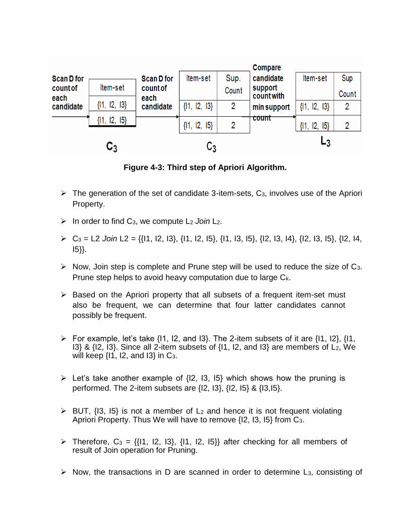
Figure 4-3: Third step of Apriori Algorithm.

The generation of the set of candidate 3-item-sets, C3, involves use of the Apriori

Property.

In order to find C3, we compute L2 Join L2.

C3 = L2 Join L2 = {{I1, I2, I3}, {I1, I2, I5}, {I1, I3, I5}, {I2, I3, I4}, {I2, I3, I5}, {I2, I4,

I5}}.

Now, Join step is complete and Prune step will be used to reduce the size of C3.

Prune step helps to avoid heavy computation due to large Ck.

Based on the Apriori property that all subsets of a frequent item-set must

also be frequent, we can determine that four latter candidates cannot

possibly be frequent.

For example, let’s take {I1, I2, and I3}. The 2-item subsets of it are {I1, I2}, {I1, I3} & {I2, I3}. Since all 2-item subsets of {I1, I2, and I3} are members of L2, We will keep {I1, I2, and I3} in C3.

Let’s take another example of {I2, I3, I5} which shows how the pruning is

performed. The 2-item subsets are {I2, I3}, {I2, I5} & {I3,I5}.

BUT, {I3, I5} is not a member of L2 and hence it is not frequent violating Apriori Property. Thus We will have to remove {I2, I3, I5} from C3.

Therefore, C3 = {{I1, I2, I3}, {I1, I2, I5}} after checking for all members of result of Join operation for Pruning.

Now, the transactions in D are scanned in order to determine L3, consisting of

those candidates 3-item-sets in C3 having minimum support.

Step 4: Generating 4-item-set Frequent Pattern

The algorithm uses L3 Join L3 to generate a candidate set of 4-item-sets, C4.

Although the join results in {{I1, I2, I3, I5}}, this item-set is pruned since its subset

{{I2, I3, I5}} is not frequent.

Thus, C4 = φ, and algorithm terminates, having found all of the frequent items.

This completes our Apriori Algorithm.

These frequent item-sets will be used to generate strong association rules (where

strong association rules satisfy both minimum support & minimum confidence).

Step 5: Generating Association Rules from Frequent

Item-sets

Procedure:

For each frequent item-set “l”, generate all nonempty subsets of l.

For every nonempty subset s of l, output the rule “s (l-s)” if

support_count(l) / support_count(s) >= min_conf where min_conf is

minimum confidence threshold.

Back To Example:

We had L = {{I1}, {I2}, {I3}, {I4}, {I5}, {I1,I2}, {I1,I3}, {I1,I5}, {I2,I3}, {I2,I4}, {I2,I5},

{I1,I2,I3}, {I1,I2,I5}}.

Let’s take l = {I1,I2,I5}.

It’s all nonempty subsets are {I1,I2}, {I1,I5}, {I2,I5}, {I1}, {I2}, {I5}.

Let minimum confidence threshold is , say 70%. The resulting association rules are shown below, each listed with its confidence.

R1: I1 ^ I2 I5

Confidence = sc{I1,I2,I5}/sc{I1,I2} = 2/4 = 50% R1 is Rejected.

R2: I1 ^ I5 I2

Confidence = sc{I1,I2,I5}/sc{I1,I5} = 2/2 = 100% R2 is Selected.

R3: I2 ^ I5 I1

Confidence = sc{I1,I2,I5}/sc{I2,I5} = 2/2 = 100% R3 is Selected.

R4: I1 I2 ^ I5

Confidence = sc{I1,I2,I5}/sc{I1} = 2/6 = 33%

R4 is Rejected.

R5: I2 I1 ^ I5

Confidence = sc{I1,I2,I5}/{I2} = 2/7 = 29%

R5 is Rejected.

R6: I5 I1 ^ I2

Confidence = sc{I1,I2,I5}/ {I5} = 2/2 = 100%

R6 is Selected.

In this way, We have found three strong association rules.

4.1.6 Methods to Improve Apriori’s Efficiency

Hash-based item-set counting: A k-item-set whose corresponding hashing bucket

count is below the threshold cannot be frequent.

Transaction reduction: A transaction that does not contain any frequent k-item-

set is useless in subsequent scans.

Partitioning: Any item-set that is potentially frequent in DB must be frequent in at

least one of the partitions of DB.

Sampling: mining on a subset of given data, lower support threshold + a method

to determine the completeness.

Dynamic item-set counting: add new candidate item-sets only when all of their

subsets are estimated to be frequent.

4.1.7 Principle

Downward closure property.

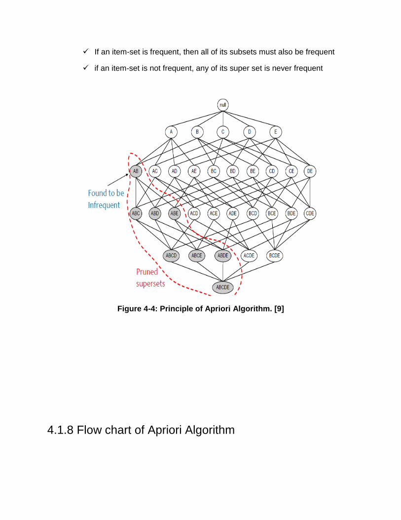
If an item-set is frequent, then all of its subsets must also be frequent

if an item-set is not frequent, any of its super set is never frequent

Figure 4-4: Principle of Apriori Algorithm. [9]

4.1.8 Flow chart of Apriori Algorithm

Figure 4-5: Flow chart of Apriori Algorithm. [10]

4.1.9 Hash based method of Apriori Algorithm

Repeat //for each transaction of the database

{

D = { set of all possible k-item-sets in the ith transaction}

For each element of D

{

Find a unique integer uniq_int using the hash function for k-item-set

Increment freq[uniq_int]

}

Increment trans_pos

//Moves pointer to next transaction until end_of_file

For (freq_ind=0; freq_ind<length_of_the_array(two_three_freq[]); freq_ind++)

{

if (freq[freq_ind] >= required support)

mark the corresponding k-item-set

}

}

4.1.10 Graph based approach

Procedure FrequentItemGraph (Tree, F)

{

scan the DB once to collect the frequent 2-itemsets

and their support ascending;

add all items in the DB as the header nodes

for each 2-itemset entry (top down order) in freq2list

do

if (first item = item in header node) then

create a link to the corresponding header node i=3

for each i-item-sets entry in the tree

do

call buildsubtree (F)

end }

Procedure buildsubtree (F)

If (first i-1 item-set = item-sets in their respective header nodes) then

create a link to the corresponding header node i=i+1

repeat buildsubtree (F)

end }

4.1.11 Performance

To assess the relative performance of the algorithms for discovering large sets, we

performed several experiments on an IBM RS/6000 530H workstation with a CPU clock

rate of 33 MHz, 64 MB of main memory, and running AIX 3.2. The data resided in the

AIXle system and was stored on a 2GB SCSI3.5" drive, with measured sequential

throughput of about 2 MB/second. [11]

We give an overview of the AIS [12] and SETM [13] algorithms against which we

compare the performance of the Apriori and Apriori Tid algorithms.

We then describe the synthetic datasets used in the performance evaluation and show

the performance results. Finally, we describe how the best performance features of

Apriori and Apriori Tid can be combined into an Apriori Hybrid algorithm and

demonstrate its scale-up properties.

4.1.12 Problem

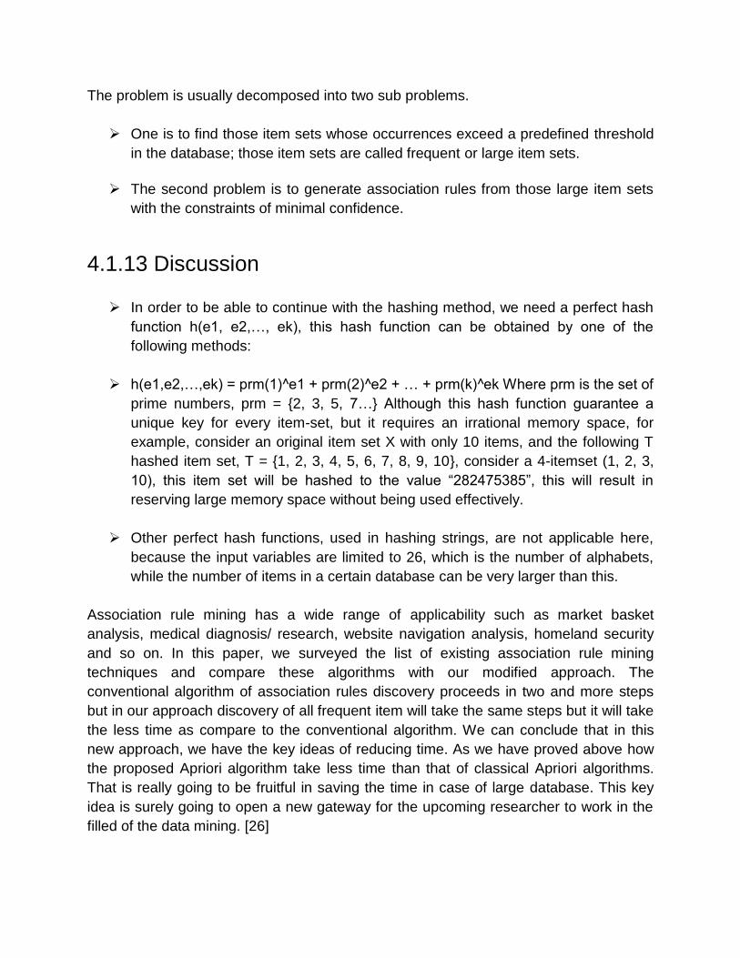
The problem is usually decomposed into two sub problems.

One is to find those item sets whose occurrences exceed a predefined threshold

in the database; those item sets are called frequent or large item sets.

The second problem is to generate association rules from those large item sets

with the constraints of minimal confidence.

4.1.13 Discussion

In order to be able to continue with the hashing method, we need a perfect hash

function h(e1, e2,…, ek), this hash function can be obtained by one of the

following methods:

h(e1,e2,…,ek) = prm(1)^e1 + prm(2)^e2 + … + prm(k)^ek Where prm is the set of

prime numbers, prm = {2, 3, 5, 7…} Although this hash function guarantee a

unique key for every item-set, but it requires an irrational memory space, for

example, consider an original item set X with only 10 items, and the following T

hashed item set, T = {1, 2, 3, 4, 5, 6, 7, 8, 9, 10}, consider a 4-itemset (1, 2, 3,

10), this item set will be hashed to the value “282475385”, this will result in

reserving large memory space without being used effectively.

Other perfect hash functions, used in hashing strings, are not applicable here,

because the input variables are limited to 26, which is the number of alphabets,

while the number of items in a certain database can be very larger than this.

Association rule mining has a wide range of applicability such as market basket

analysis, medical diagnosis/ research, website navigation analysis, homeland security

and so on. In this paper, we surveyed the list of existing association rule mining

techniques and compare these algorithms with our modified approach. The

conventional algorithm of association rules discovery proceeds in two and more steps

but in our approach discovery of all frequent item will take the same steps but it will take

the less time as compare to the conventional algorithm. We can conclude that in this

new approach, we have the key ideas of reducing time. As we have proved above how

the proposed Apriori algorithm take less time than that of classical Apriori algorithms.

That is really going to be fruitful in saving the time in case of large database. This key

idea is surely going to open a new gateway for the upcoming researcher to work in the

filled of the data mining. [26]

Use hashing techniques to find the efficient frequent 2-item-sets in order to reduce the

time and memory requirements to build a graphical structure.

4.2 FP-Growth Algorithm

One of the currently fastest and most popular algorithms for frequent item set mining is

the FP-growth algorithm [27]. It is based on a prefix tree representation of the given

database of transactions (called an FP-tree), which can save considerable amounts of

memory for storing the transactions. Our thesis work is based on FP-Growth Algorithm

a Suffix tree representation.

The basic idea of the FP-growth algorithm can be described as a recursive elimination

scheme: in a preprocessing step delete all items from the transactions that are not

frequent individually, i.e., do not appear in a user-specified minimum number of

transactions. Then select all transactions that contain the least frequent item (least

frequent among those that are frequent) and delete this item from them.

On return, remove the processed item also from the database of all transactions and

start over, i.e., process the second frequent item etc. In these processing steps the

prefix tree, which is enhanced by links between the branches, is exploited to quickly find

the transactions containing a given item and also to remove this item from the

transactions after it has been processed.

The FP-Growth Algorithm is an alternative way to find frequent item-sets without using candidate generations, thus improving performance. For so much it uses a divide-and-conquer strategy. The core of this method is the usage of a special data structure named frequent-pattern tree (FP-tree), which retains the item-set association information.

In simple words, this algorithm works as follows: first it compresses the input database creating an FP-tree instance to represent frequent items. After this first step it divides the compressed database into a set of conditional databases, each one associated with one frequent pattern. Finally, each such database is mined separately. Using this strategy, the FP-Growth reduces the search costs looking for short patterns recursively and then concatenating them in the long frequent patterns, offering good selectivity.

In large databases, it’s not possible to hold the FP-tree in the main memory. A strategy to cope with this problem is to firstly partition the database into a set of smaller databases (called projected databases), and then construct an FP-tree from each of these smaller databases.

4.2.1 Preprocessing

Similar to several other algorithms for frequent item set mining, like, for example,

Apriori, FP-growth preprocesses the transaction database as follows: in an initial scan

the frequencies of the items (support of single element item-sets) are determined. All

infrequent items—that is, all items that appear in fewer transactions than a user-

specified minimum number—are discarded from the transactions, since, obviously, they

can never be part of a frequent item set.

In addition, the items in each transaction are sorted, so that they are in descending

order W.R.T. their frequency in the database. Although the algorithm does not depend

on this specific order, experiments showed that it leads to much shorter execution times

than a random order. An ascending order leads to a particularly slow operation in my

experiments, performing even worse than a random order.

This preprocessing is demonstrated in Table 5-1, which shows an example transaction

database on the left. The frequencies of the items in this database, sorted descendingly,

are shown in the middle of this table. If we are given a user specified minimal support of

3 transactions, items f and g can be discarded. After doing so and sorting the items in

each transaction descending W.R.T. their frequencies we obtain the reduced database

shown in Table 5-1 on the right.

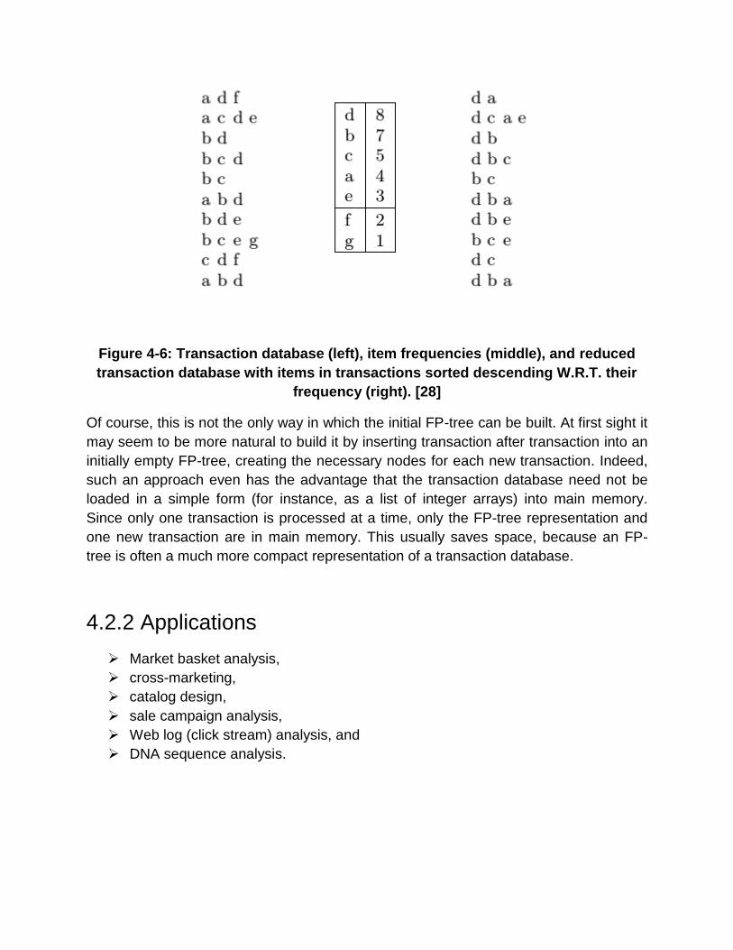
Figure 4-6: Transaction database (left), item frequencies (middle), and reduced

transaction database with items in transactions sorted descending W.R.T. their

frequency (right). [28]

Of course, this is not the only way in which the initial FP-tree can be built. At first sight it

may seem to be more natural to build it by inserting transaction after transaction into an

initially empty FP-tree, creating the necessary nodes for each new transaction. Indeed,

such an approach even has the advantage that the transaction database need not be

loaded in a simple form (for instance, as a list of integer arrays) into main memory.

Since only one transaction is processed at a time, only the FP-tree representation and

one new transaction are in main memory. This usually saves space, because an FP-

tree is often a much more compact representation of a transaction database.

4.2.2 Applications

Market basket analysis,

cross-marketing,

catalog design,

sale campaign analysis,

Web log (click stream) analysis, and

DNA sequence analysis.

4.2.3 FP-Growth Method: Construction of FP-Tree

First, create the root of the tree, labeled with “null”.

Scan the database D a second time. (First time we scanned it to create 1-itemset

and then L).

The items in each transaction are processed in L order (i.e. sorted order).

A branch is created for each transaction with items having their support count

separated by colon.

Whenever the same node is encountered in another transaction, we just

increment the support count of the common node or Prefix.

To facilitate tree traversal, an item header table is built so that each item points to

its occurrences in the tree via a chain of node-links.

Now, the problem of mining frequent patterns in database is transformed to that of

mining the FP-Tree.

4.2.4 Mining the FP-Tree by Creating Conditional (sub)

pattern bases

Steps:

Start from each frequent length-1 pattern (as an initial suffix pattern).

Construct its conditional pattern base which consists of the set of prefix paths in

the FP-Tree co-occurring with suffix pattern.

Then, Construct its conditional FP-Tree & perform mining on such a tree.

The pattern growth is achieved by concatenation of the suffix pattern with the

frequent patterns generated from a conditional FP-Tree.

The union of all frequent patterns (generated by step 4) gives the required

frequent item-set.

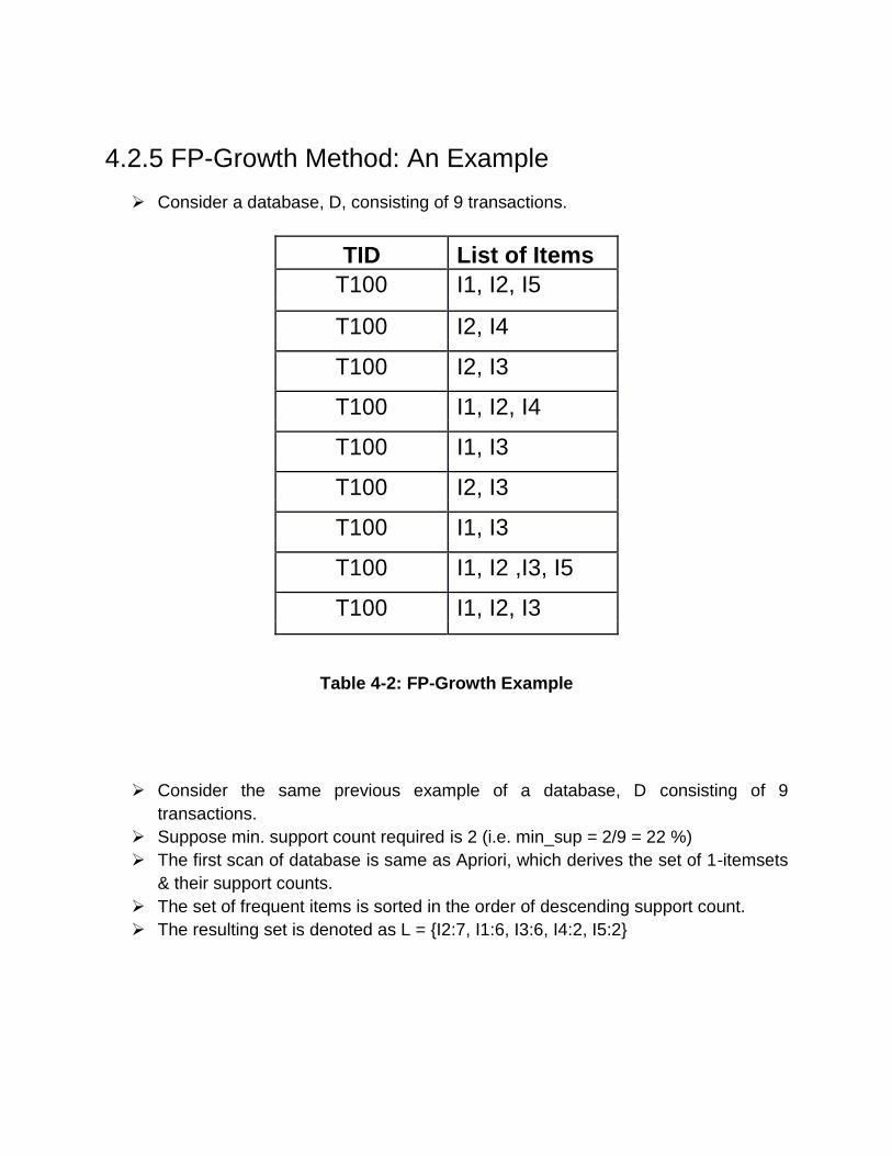
4.2.5 FP-Growth Method: An Example

Consider a database, D, consisting of 9 transactions.

TID List of Items

T100 I1, I2, I5

T100 I2, I4

T100 I2, I3

T100 I1, I2, I4

T100 I1, I3

T100 I2, I3

T100 I1, I3

T100 I1, I2 ,I3, I5

T100 I1, I2, I3

Table 4-2: FP-Growth Example

Consider the same previous example of a database, D consisting of 9

transactions.

Suppose min. support count required is 2 (i.e. min_sup = 2/9 = 22 %)

The first scan of database is same as Apriori, which derives the set of 1-itemsets

& their support counts.

The set of frequent items is sorted in the order of descending support count.

The resulting set is denoted as L = {I2:7, I1:6, I3:6, I4:2, I5:2}

FP-Growth Method: Construction of FP-Tree

Figure 4-7: An FP-Tree that registers compressed, frequent pattern information

[45]

Item Conditional pattern base Conditional

FP-Tree

Frequent pattern generated

I5 {(I2 I1: 1),(I2 I1 I3: 1)} <I2:2 , I1:2> I2 I5:2, I1 I5:2, I2 I1 I5: 2

I4 {(I2 I1: 1),(I2: 1)} <I2: 2> I2 I4: 2

I3 {(I2 I1: 1),(I2: 2), (I1: 2)} <I2: 4, I1: 2>,<I1:2> I2 I3:4, I1, I3: 2 , I2 I1 I3: 2

I2 {(I2: 4)} <I2: 4> I2 I1: 4

Table 4-3 : Mining the FP-Tree by creating conditional (sub) pattern bases

4.2.6 Advantages of FP-Growth

Only 2 pass over data-set.

“Compresses” data-set.

No candidate generation.

Much faster than Apriori.

4.2.7 Disadvantages of FP-Growth

FP-Tree may not fit in memory.

FP-Tree is expensive to build.

4.2.8 Why Frequent Pattern Growth Fast

Performance study shows

FP-growth is an order of magnitude faster than Apriori, and is also faster than

tree-projection

Reasoning

No candidate generation, no candidate test

Use compact data structure

Eliminate repeated database scan

Basic operation is counting and FP-tree building

4.3 Prefix Tree

In computer science, a trie, also called digital tree and sometimes radix tree or prefix

tree (as they can be searched by prefixes), is an ordered tree data structure that is used

to store a dynamic set or associative array where the keys are usually strings. Unlike a

binary search tree, no node in the tree stores the key associated with that node;

instead, its position in the tree defines the key with which it is associated. All the

descendants of a node have a common prefix of the string associated with that node,

and the root is associated with the empty string. Values are normally not associated

with every node, only with leaves and some inner nodes that correspond to keys of

interest.

The term trie comes from retrieval. This term was coined by Edward Fredkin. However,

other authors pronounce it /ˈtraɪ/ "try", in an attempt to distinguish it verbally from

"tree".[29] [30]

In the example shown, keys are listed in the nodes and values below them. Each

complete English word has an arbitrary integer value associated with it. A trie can be

seen as a deterministic finite automaton without loops. Each finite language is

generated by a trie automaton, and each trie can be compressed into a DAFSA.

It is not necessary for keys to be explicitly stored in nodes. (In the figure, words are

shown only to illustrate how the trie works.)

Though tries are most commonly keyed by character strings, they don't need to be. The

same algorithms can easily be adapted to serve similar functions of ordered lists of any

construct, e.g., permutations on a list of digits or shapes. In particular, a bitwise trie is

keyed on the individual bits making up a short, fixed size of bits such as an integer

number or memory address.

4.4 Suffix Tree

In computer science, a suffix tree (also called PAT tree or, in an earlier form, position

tree) is a compressed trie containing all the suffixes of the given text as their keys and

positions in the text as their values. Suffix trees allow particularly fast implementations

of many important string operations.

The construction of such a tree for the string S takes time and space linear in the length

of S. Once constructed, several operations can be performed quickly, for instance

locating a substring in S, locating a substring if a certain number of mistakes are

allowed, locating matches for a regular expression pattern etc. Suffix trees also

provided one of the first linear-time solutions for the longest common substring problem.

These speedups come at a cost: storing a string's suffix tree typically requires

significantly more space than storing the string itself.

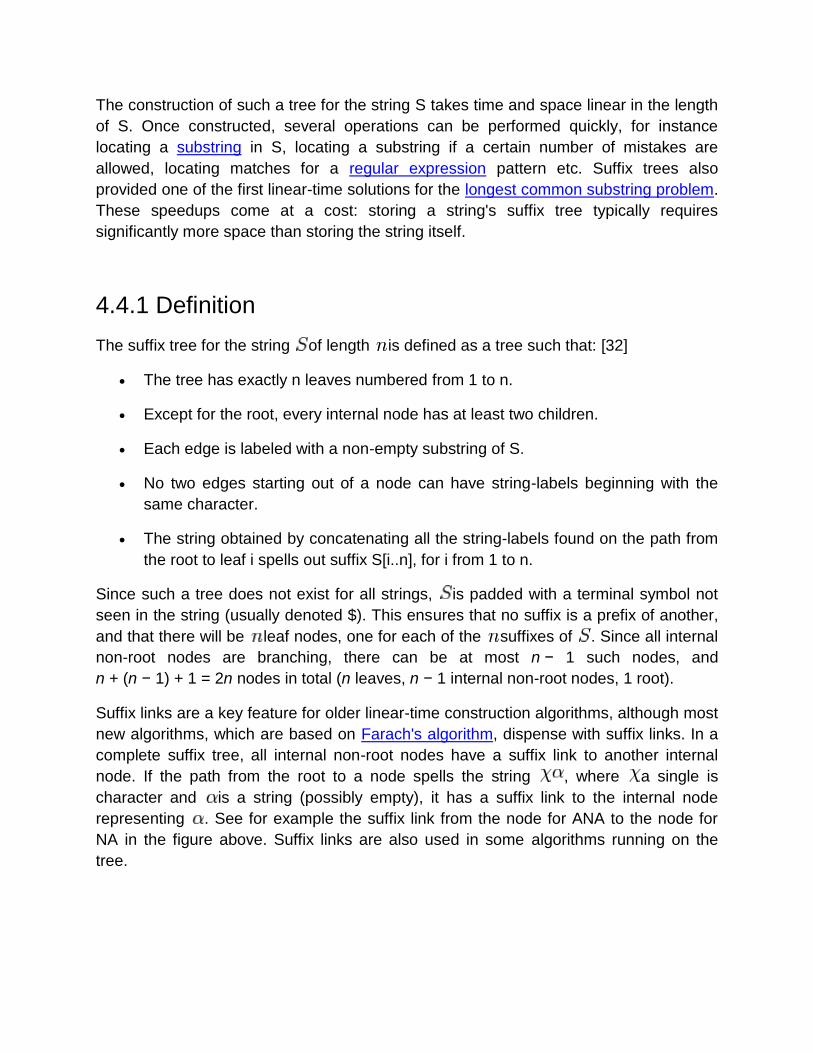
4.4.1 Definition

The suffix tree for the string of length is defined as a tree such that: [32]

The tree has exactly n leaves numbered from 1 to n.

Except for the root, every internal node has at least two children.

Each edge is labeled with a non-empty substring of S.

No two edges starting out of a node can have string-labels beginning with the

same character.

The string obtained by concatenating all the string-labels found on the path from

the root to leaf i spells out suffix S[i..n], for i from 1 to n.

Since such a tree does not exist for all strings, is padded with a terminal symbol not

seen in the string (usually denoted $). This ensures that no suffix is a prefix of another,

and that there will be leaf nodes, one for each of the suffixes of . Since all internal

non-root nodes are branching, there can be at most n − 1 such nodes, and

n + (n − 1) + 1 = 2n nodes in total (n leaves, n − 1 internal non-root nodes, 1 root).

Suffix links are a key feature for older linear-time construction algorithms, although most

new algorithms, which are based on Farach's algorithm, dispense with suffix links. In a

complete suffix tree, all internal non-root nodes have a suffix link to another internal

node. If the path from the root to a node spells the string , where a single is

character and is a string (possibly empty), it has a suffix link to the internal node

representing . See for example the suffix link from the node for ANA to the node for

NA in the figure above. Suffix links are also used in some algorithms running on the

tree.

4.4.2 Applications

Suffix trees can be used to solve a large number of string problems that occur in text-

editing, free-text search, computational biology and other application areas. Primary

applications include: [33]

String search, in O(m) complexity, where m is the length of the sub-string (but

with initial O(n) time required to build the suffix tree for the string)

Finding the longest repeated substring

Finding the longest common substring

Finding the longest palindrome in a string

Suffix trees are often used in bioinformatics applications, searching for patterns in DNA

or protein sequences (which can be viewed as long strings of characters). The ability to

search efficiently with mismatches might be considered their greatest strength. Suffix

trees are also used in data compression; they can be used to find repeated data, and

can be used for the sorting stage of the Burrows–Wheeler transform. Variants of the

LZW compression schemes use suffix trees (LZSS). A suffix tree is also used in suffix

tree clustering, a data clustering algorithm used in some search engines. [34]

4.4.3 Functionality

A suffix tree for a string of length can be built in time, if the letters come from

an alphabet of integers in a polynomial range (in particular, this is true for constant-

sized alphabets). [35] For larger alphabets, the running time is dominated by first sorting

the letters to bring them into a range of size ; in general, this takes

time. The costs below are given under the assumption that the alphabet is constant.

Assume that a suffix tree has been built for the string of length , or that a

generalized suffix tree has been built for the set of strings of

total length . You can:

Search for strings:

Check if a string of length is a substring in time. [36]

Find the first occurrence of the patterns of total length as

substrings in time.

Find all occurrences of the patterns of total length as

substrings in time.

Search for a regular expression P in time expected sub linear in . [ 37]

Find for each suffix of a pattern , the length of the longest match

between a prefix of and a substring in in time. This is

termed the matching statistics for .

Find properties of the strings:

Find the longest common substrings of the string and in

time.

Find all maximal pairs, maximal repeats or super maximal repeats in

time.

Find the Lempel–Ziv decomposition in time.

Find the longest repeated substrings in time.

Find the most frequently occurring substrings of a minimum length in

time.

Find the shortest strings from that do not occur in , in time,

if there are such strings.

Find the shortest substrings occurring only once in time.

Find, for each , the shortest substrings of not occurring elsewhere in

in time.

The suffix tree can be prepared for constant time lowest common ancestor retrieval

between nodes in time.[11] One can then also:

Find the longest common prefix between the suffixes and in

.

Search for a pattern P of length m with at most k mismatches in

time, where z is the number of hits.[13]

Find all maximal palindromes in ,[14] or time if gaps of length are

allowed, or if mismatches are allowed.[15]

Find all tandem repeats in , and k-mismatch tandem repeats in

.

Find the longest substrings common to at least string in for in

time.

Find the longest palindrome substring of a given string (using the suffix trees of

both the string and its reverse) in linear time. [38]

4.5 Related Work

Mining of frequent itemsets is an important phase in association mining which discovers

frequent itemsets in transactions database. It is the core in many tasks of data mining

that try to find interesting patterns from datasets, such as association rules, episodes,

classifier, clustering and correlation, etc [43]. Many algorithms are proposed to find

frequent itemsets, but all of them can be catalogued into two classes: candidate

generation or pattern growth.

Apriori [44] is a representative the candidate generation approach. It generates length

(k+1) candidate itemsets based on length (k) frequent itemsets. The frequency of

itemsets is defined by counting their occurrence in transactions. FP-growth, is proposed

by Han in 2000, represents pattern growth approach, it used specific data structure (FP-

tree), FP-growth discover the frequent itemsets by finding all frequent in 1-itemsets into

condition pattern base , the condition pattern base is constructed efficiently based on

the link of node structure that association with FP-tree. FP-growth does not generate

candidate itemsets explicitly.

Chapter 5

The Proposed Algorithm

In this paper we proposed a frequent pattern mining algorithm using suffix automata,

which is a modified algorithm of the Ukkonen’s Algorithm.

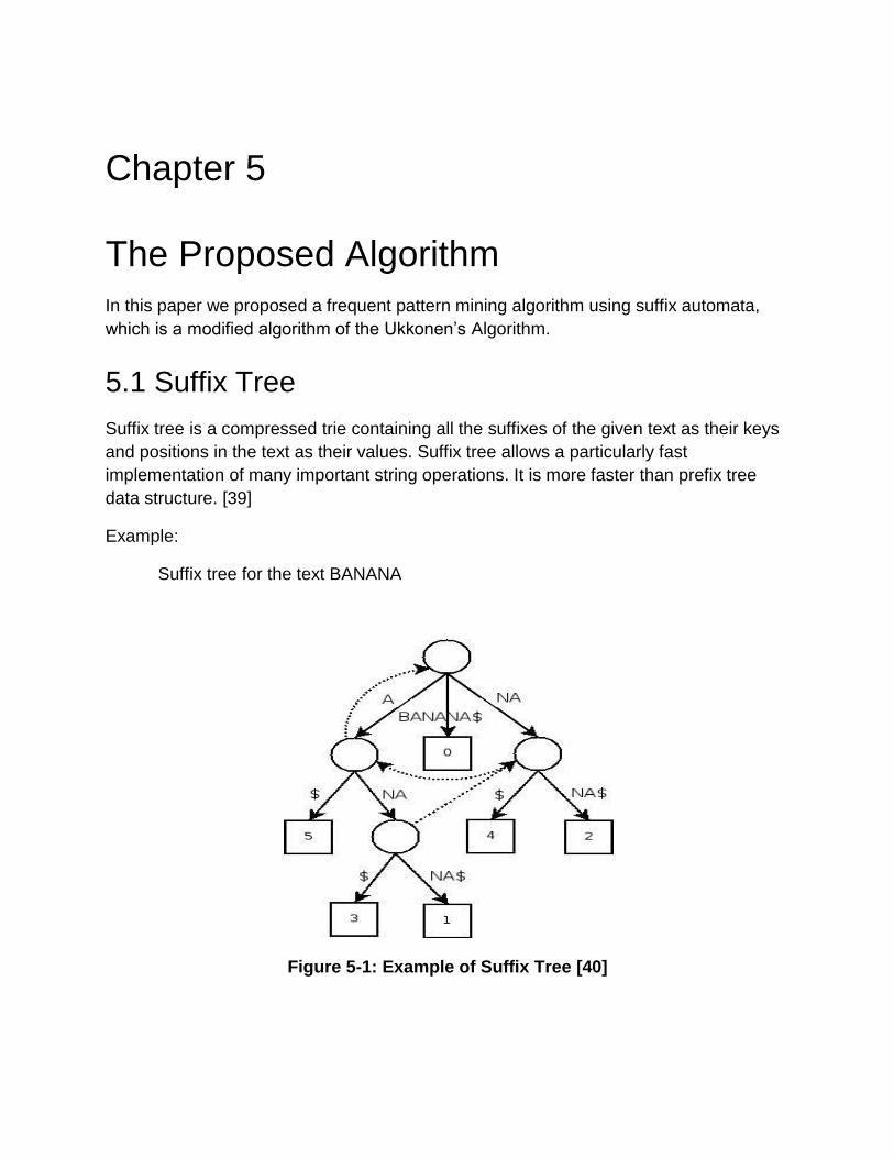
5.1 Suffix Tree

Suffix tree is a compressed trie containing all the suffixes of the given text as their keys

and positions in the text as their values. Suffix tree allows a particularly fast

implementation of many important string operations. It is more faster than prefix tree

data structure. [39]

Example:

Suffix tree for the text BANANA

Figure 5-1: Example of Suffix Tree [40]

5.2 Ukkonen's algorithm

In computer science, Ukkonen's algorithm is a linear-time, online algorithm for

constructing suffix trees, proposed by Esko Ukkonen in 1995.

The algorithm begins with an implicit suffix tree containing the first character of the

string. Then it steps through the string adding successive characters until the tree is

complete. This order addition of characters gives Ukkonen's algorithm its "on-line"

property. Earlier algorithms proceeded backward from the last character to the first one,

let it be from the longest to the shortest suffix or from the shortest to the longest

suffix.[3] The naive implementation for generating a suffix tree requires O(n2) or even

O(n3) time, where n is the length of the string. By exploiting a number of algorithmic

techniques, Ukkonen reduced this to O(n) (linear) time, for constant-size alphabets, and

O(n log n) in general. [41]

5.3 Suffix automata

Suffix automata and factor automata are efficient data structures for representing the full

index of a set of strings. They are minimal deterministic automata representing the set

of all suffixes or substrings of a set of strings. The suffix automation of a string u is the

minimal deterministic finite automation recognizing the set of suffixes of u. Its size is

linear in the length of u, n.

Figure 5-2: (a) A deterministic finite automation A and (b) a deterministic

automation recognizing ∑*L(A) where transitions labeled with φ are failure

transitions.

More precisely , its number of states between n & 2n-1 and its number of transitions

between n+1 & 3n-2. This automation can be obtained by minimizing the suffix trie of u.

A crucial advantage of suffix automata is that , unlike suffix trees they do not require the

use of compact transitions for the size to be linear to |u|. [42]

5.4 Algorithm

Create prefix paths for a particular suffix node. This is done by gathering all the paths containing a particular suffix node. Any path that ends with this suffix is examined.

Using the prefix path tree determine whether the suffix is frequent. This is done by adding the support counts associated with the node and if the number is greater than or equal to the min_sup (minimum support) the node is frequent. If the node isn’t frequent the analysis ends for this suffix.

Convert the prefix paths into a conditional FP-tree.

I. Update the support counts along the prefix paths to reflex the actual number of transactions containing the item-set

II. Truncate the prefix paths by removing the nodes of the chosen suffix

III. Remove items that may no longer be frequent (if the support count of a particular node is less than min_sup it is no longer frequent and should be pruned).

IV. Repeat I →III for all prefix paths for the chosen suffix.

Repeat Steps 1-3 for all suffix nodes to determine the frequent item-set for the dataset.

5.5 Procedure

Step 1: Given word sequence to be searched is tokenized first.

Step 2: Initialized n to 1

Search the nodes of root for first token

If there is a match

Performs step3

Else

If n is last node of root+1

Return search failed

Else

Increment n and again search with next node of root

Step 3: Consider only the level 1 nth node sub tree

Compare next token with level 2 first node

Do{

If there is a match

I. Perform depth first search traversal on the tree comparing with

remaining tokens

II. Applying k- mismatch retrieve the documents that contain the word

sequence

Else

If all the level 1 nth node sub tree nodes are traversed word

sequence is not present

Else

Apply k- mismatch, perform DFS traversal and compare with

the next token

}

While all the tokens of word are not completed or entire level 1 nth node sub tree

nodes are not traversed.

Example:

Let, Minimum Support 2

T1- CDAB

T2-CDB

T3-CDA

Build Tree

Figure 5-3: Contraction of Build Tree

B-1

9

CD-3

5

Root

1

B-2

2

A-2

6

B-1

7

D-3

4 B-1

10

A-2

3

B-1

12

B-1

11

A-2

8

Sub-tree of B

Figure 5-4: Frequent Pattern is B(2).

Sub-tree of A

Figure 5-5: Frequent Pattern is A(2).

Sub-tree of D

Figure 5-6: Frequent Pattern is D(3), DA(2), DB(2).

B-2

2

A-2

2

B-1

10

D-3

4

B-1

7

D-3

4

A-2

6 A-2

6

B-2

7

B-1

11

B-1

11

Sub-tree of CD

Figure 5-7: Frequent Pattern is C(3), CD(3), CB(2), CA(2), CDA(2).

B-2

14

B-1

16

A-2

15

D-3

13

C-3

5 B-1

9

A-2

8

B-1

12

CD-3

5

A-2

8

B-1

9

B-1

12

Chapter 6

Performances Analysis

This chapter presents results and performance comparison with this algorithm and

some previous algorithms. Before the performance analysis complexity analysis will be

discussed briefly.

6.1 Complexity Analysis

As described before, we see that naive implementation for generating a suffix tree or a

prefix tree requires O(n^2) time, where n is the length of the string. But we use

Ukkonen’s algorithms techniques which reduce the time complexity to O(n) time.

[39][41][29][30]

Data structure Time complexity

Suffix (naïve) O(n^2)

Prefix O(n^2)

Suffix(Ukkonen) O(n)

Table 6-1: Complexity Analysis

6.2 Environments of Experiments All the experiments are performed on a Intel ® Core™ Duo CPU 2.93GHz PC machine with 2GB main memory, running on Microsoft Windows 7. All the programs are written in Java. Notice that we do not directly compare our absolute number of runtime with those in some published reports running on the RISC workstations because different machine architectures may differ greatly on the absolute runtime for the same algorithms. Instead, we implement their algorithms to the best of our knowledge based on the published reports on the same machine and compare in the same running environment. Please also note that run time used here means the total execution time, that is, the period between input and output, instead of CPU time measured in the experiments in some literature. We feel that run time is a more comprehensive measure since it takes the total running time consumed as the measure of cost, whereas CPU time considers only the cost of the CPU resource. The experiments are pursued on both synthetic and real data sets. The synthetic data sets which we used for our experiments

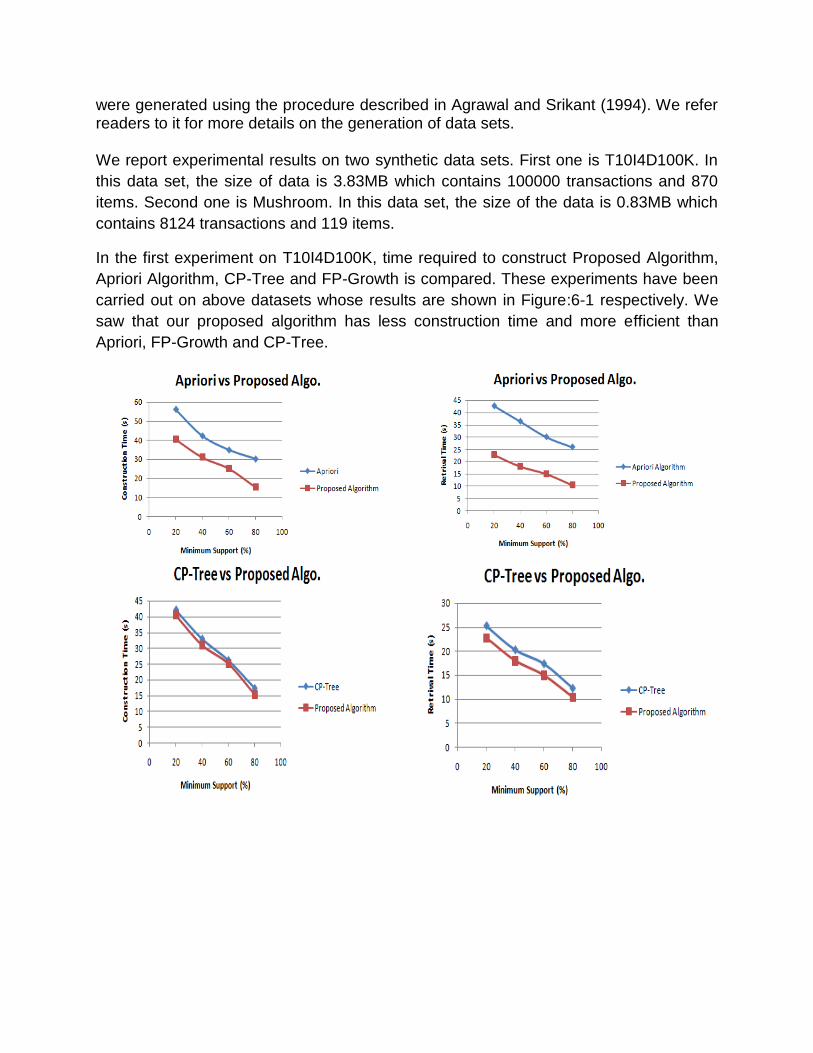
were generated using the procedure described in Agrawal and Srikant (1994). We refer readers to it for more details on the generation of data sets. We report experimental results on two synthetic data sets. First one is T10I4D100K. In

this data set, the size of data is 3.83MB which contains 100000 transactions and 870

items. Second one is Mushroom. In this data set, the size of the data is 0.83MB which

contains 8124 transactions and 119 items.

In the first experiment on T10I4D100K, time required to construct Proposed Algorithm,

Apriori Algorithm, CP-Tree and FP-Growth is compared. These experiments have been

carried out on above datasets whose results are shown in Figure:6-1 respectively. We

saw that our proposed algorithm has less construction time and more efficient than

Apriori, FP-Growth and CP-Tree.

Figure 6-1: Comparison between Apriori, FP-Growth, CP-Tree & Proposed

Algorithm on T10I4D100K Data.

In the second experiment on Mushroom, time required to construct Proposed Algorithm,

Apriori Algorithm, CP-Tree and FP-Growth is compared. These experiments have been

carried out on above datasets whose results are shown in Figure:6-2 respectively. We

saw that our proposed algorithm has less construction time and more efficient than

Apriori, FP-Growth and CP-Tree.

Figure 6-2: Comparison between Apriori, FP-Growth, CP-Tree & Proposed

Algorithm on Mushroom Data Set.

Chapter 7

Conclusion

Mining frequent item-sets for the association rule mining from the large transactional

database is a very crucial task. There are many approaches that have been discussed;

nearly all of the previous studies were using Apriori approach and FP-Tree approach for

extracting the frequent item-sets, which have scope for improvement. Thus the goal of

this research was to find a scheme for pulling the rules out of the transactional data sets

considering the time and the memory consumption. This chapter summarizes the work

done in this thesis and then the future scope is given.

In this thesis, we considered the following factors for creating our new scheme, which

are the time and the memory consumption, these factors are affected by the approach

for finding the frequent item-sets. Work has been done to develop an algorithm which is

an improvement over Apriori and FP-tree with using an approach of improved Apriori

and FP-Tree algorithm for a transactional database. According to our observations, the

performances of the algorithms are strongly depends on the support levels and the

features of the data sets (the nature and the size of the data sets). Therefore we

employed it in our scheme to guarantee the time saving and the memory in the case of

sparse and dense data sets. It is found that for a transactional database where many

transaction items are repeated many times as a super set in that type of database

maximal Apriori (improvement over classical Apriori) is best suited for mining frequent

item-sets. The item-sets which are not included in maximal super set are treated by FP-

tree for finding the remaining frequent item-sets. Thus this algorithm produces frequent

item-sets completely. This approach doesn’t produce candidate item-sets and building

FP-tree only for pruned database that fit into main memory easily. Thus it saves much

time and space and considered as an efficient method as proved from the results. For

both data sets the running time and memory consumption of our new scheme

outperformed Apriori. Whereas the running time of our scheme performed well over the

FP-growth on the collected data set at the lower support level where probability of

finding maximal frequent item-sets is large and at higher lever running time is

approximately same as the FP-Tree. The memory consumption is also approximately

same as the FP-Tree at higher support and performed well at lower support.

The main contributions of this Thesis:

We can summarize the main contribution of this research as follows:

• To study and analyze various existing approaches to mine frequent item-sets.

• To devised a new better scheme than classical Apriori and FP-tree alone using

maximal Apriori and FP-tree as combined approach for mining frequent item-sets.

7.1 Future Trends

There are a number of future work directions based on the work presented in this thesis.

Using constraints can further reduce the size of item-sets generated and

improve mining efficiency.

This scheme was applied in retailer industry application, trying other

industry is an interesting field for future work.

This scheme use Maximal Apriori and FP-Tree. We can use other

combination to improve this approach.

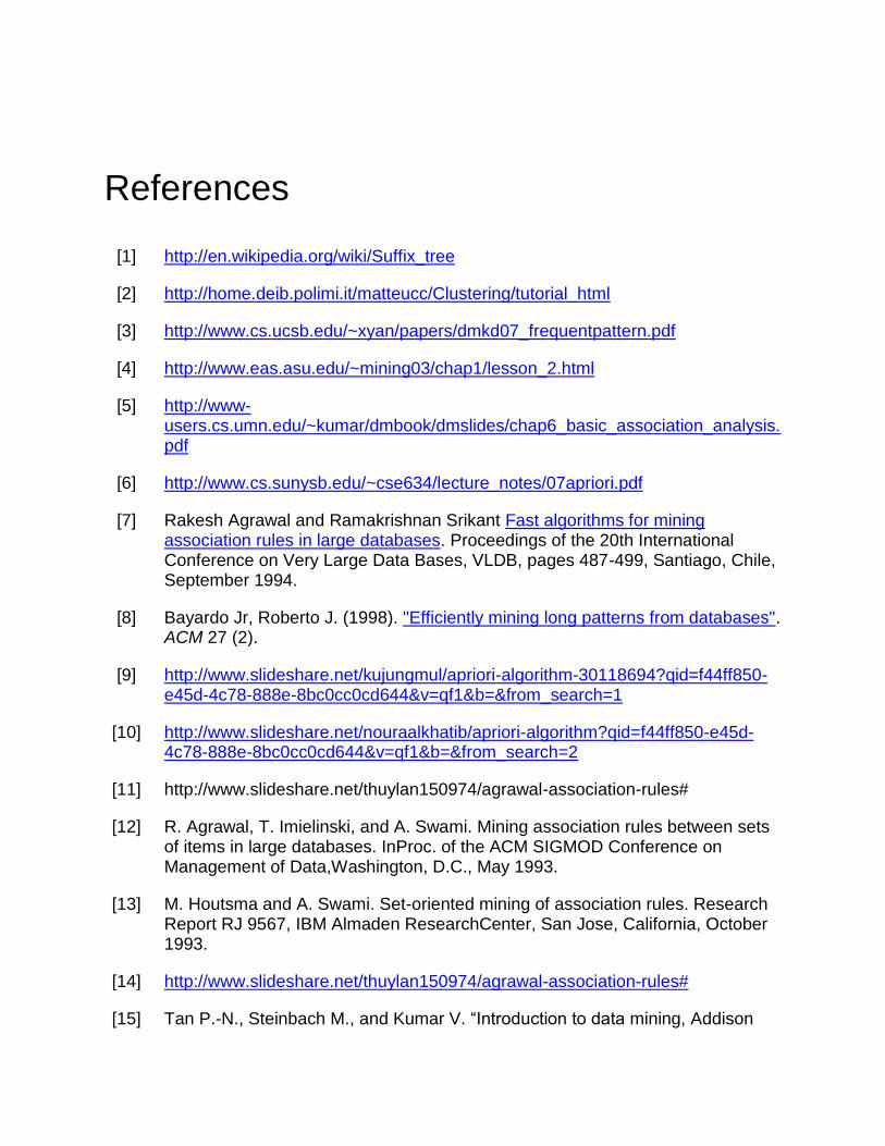
References

[1] http://en.wikipedia.org/wiki/Suffix_tree

[2] http://home.deib.polimi.it/matteucc/Clustering/tutorial_html

[3] http://www.cs.ucsb.edu/~xyan/papers/dmkd07_frequentpattern.pdf

[4] http://www.eas.asu.edu/~mining03/chap1/lesson_2.html

[5] http://www-users.cs.umn.edu/~kumar/dmbook/dmslides/chap6_basic_association_analysis.pdf

[6] http://www.cs.sunysb.edu/~cse634/lecture_notes/07apriori.pdf

[7] Rakesh Agrawal and Ramakrishnan Srikant Fast algorithms for mining association rules in large databases. Proceedings of the 20th International Conference on Very Large Data Bases, VLDB, pages 487-499, Santiago, Chile, September 1994.

[8] Bayardo Jr, Roberto J. (1998). "Efficiently mining long patterns from databases". ACM 27 (2).

[9] http://www.slideshare.net/kujungmul/apriori-algorithm-30118694?qid=f44ff850-e45d-4c78-888e-8bc0cc0cd644&v=qf1&b=&from_search=1

[10] http://www.slideshare.net/nouraalkhatib/apriori-algorithm?qid=f44ff850-e45d-4c78-888e-8bc0cc0cd644&v=qf1&b=&from_search=2

[11] http://www.slideshare.net/thuylan150974/agrawal-association-rules#

[12] R. Agrawal, T. Imielinski, and A. Swami. Mining association rules between sets of items in large databases. InProc. of the ACM SIGMOD Conference on Management of Data,Washington, D.C., May 1993.

[13] M. Houtsma and A. Swami. Set-oriented mining of association rules. Research Report RJ 9567, IBM Almaden ResearchCenter, San Jose, California, October 1993.

[14] http://www.slideshare.net/thuylan150974/agrawal-association-rules#

[15] Tan P.-N., Steinbach M., and Kumar V. “Introduction to data mining, Addison

Wesley Publishers”. 2006

[16] http://www.ijsce.org/attachments/File/v2i3/C0753062312.pdf

[17] http://www. kdnuggets. Com

[18] Fayyad U. M., Piatetsky-Shapiro G. and Smyth, P. “Data mining to knowledge discovery in databases, AI Magazine”. Vol. 17, No. 3, pp. 37-54, 1996

[19] Data mining Concepts and Techniques” by By Jiawei Han, Micheline Kamber, Morgan Kaufmann Publishers, 2006

[20] Luo D., Cao L., Luo C., Zhang C., and Wang W. “Towards business interestingness in actionable knowledge discovery”. IOS Press, Vol.177, pp. 101–111, 2008.

[21] Aggrawal.R, Imielinski.t, Swami.A. “Mining Association Rules between Sets of Items in Large Databases”. In Proc. Int’l Conf. of the 1993 ACM SIGMOD Conference Washington DC, USA

[22] Luo D., Cao L., Luo C., Zhang C., and Wang W. “Towards businessinterestingness in actionable knowledge discovery”. IOS Press, Vol.177, pp. 101–111, 2008

[23] Toivonen.H. “Sampling large databases for association rules”. In Proc. Int’l Conf. Very Large Data Bases (VLDB), Sept. 1996, Bombay, India, pages 134–145.

[24] Goswami D.N. et. al. / (IJCSE) International Journal on Computer Science and Engineering Vol. 02, No. 04,2010, 942-947

[25] Agrawal, R., Imielinski, T., and Swami, A. N. 1993. Mining association rules between sets of items in large databases. In Proceedings of the 1993 ACM SIGMOD International Conference on Management of Data, 207-216

[26] Goswami D.N. et. al. / (IJCSE) International Journal on Computer Science and Engineering Vol. 02, No. 04, 2010, 942-947

[27] J. Han, H. Pei, and Y. Yin. Mining Frequent Patterns without Candidate Generation. In: Proc. Conf. on the Management of Data (SIGMOD’00, Dallas, TX). ACM Press, New York, NY, USA 2000

[28] http://www.borgelt.net/papers/fpgrowth.pdf

[29] Franklin Mark Liang (1983). Word Hy-phen-a-tion By Com-put-er (Doctor of

Philosophy thesis). Stanford University. Archived from the original on 2010-05-19. Retrieved 2010-03-28

[30] Knuth, Donald (1997). "6.3: Digital Searching". The Art of Computer Programming Volume 3: Sorting and Searching (2nd ed.). Addison-Wesley. p. 492. ISBN 0-201-89685-0

[31] Baeza-Yates, Ricardo A.; Gonnet, Gaston H. (1996), "Fast text searching for regular expressions or automaton searching on tries", Journal of the ACM 43 (6): 915–936, doi:10.1145/235809.235810

[32] Barsky, Marina; Stege, Ulrike; Thomo, Alex; Upton, Chris (2008), "A new method for indexing genomes using on-disk suffix trees", CIKM '08: Proceedings of the 17th ACM Conference on Information and Knowledge Management, New York, NY, USA: ACM, pp. 649–658

[33] Allison, L. "Suffix Trees". Retrieved 2008-10-14

[34] First introduced by Zamir & Etzioni (1998).

[35] Barsky, Marina; Stege, Ulrike; Thomo, Alex; Upton, Chris (2009), "Suffix trees for very large genomic sequences", CIKM '09: Proceedings of the 18th ACM Conference on Information and Knowledge Management, New York, NY, USA: ACM

[36] Farach, Martin (1997), "Optimal Suffix Tree Construction with Large Alphabets", 38th IEEE Symposium on Foundations of Computer Science (FOCS '97), pp. 137–143.

[37] Giegerich, R.; Kurtz, S. (1997), "From Ukkonen to McCreight and Weiner: A Unifying View of Linear-Time Suffix Tree Construction", Algorithmica 19 (3): 331–353, doi:10.1007/PL00009177

[38] Zamir, Oren; Etzioni, Oren (1998), "Web document clustering: a feasibility demonstration", SIGIR '98: Proceedings of the 21st annual international ACM SIGIR conference on Research and development in information retrieval, New York, NY, USA: ACM, pp 46-54.

[39] http://en.wikipedia.org/wiki/Suffix_tree

[40] http://en.wikipedia.org/wiki/File:Suffix_tree_BANANA.svg

[41] http://en.wikipedia.org/wiki/Ukkonen%27s_algorithm

[42] http://www.cs.nyu.edu/~mohri/pub/nfac.pdf

[43] S. Rao, R. Gupta, “Implementing Improved Algorithm Over APRIORI Data Mining Association Rule Algorithm”, International Journal of Computer Science

And Technology , pp. 489-493 , Mar. 2012

[44] R. Srikant, “Fast algorithms for mining association rules and sequential patterns,” UNIVERSITY OF WISCONSIN, 1996.

[45] J. Han, J. Pei, and Y. Yin. Mining frequent patterns without candidate generation. SIGMOD’ 00.