Wright State University Wright State University

CORE Scholar CORE Scholar

Browse all Theses and Dissertations Theses and Dissertations

2011

An Exploratory Study of Mixed-Width Aisle Layouts for Order An Exploratory Study of Mixed-Width Aisle Layouts for Order

Picking in Distribution Centers Picking in Distribution Centers

Corinne H. Mowrey Wright State University

Follow this and additional works at: https://corescholar.libraries.wright.edu/etd_all

Part of the Operations Research, Systems Engineering and Industrial Engineering Commons

Repository Citation Repository Citation Mowrey, Corinne H., "An Exploratory Study of Mixed-Width Aisle Layouts for Order Picking in Distribution Centers" (2011). Browse all Theses and Dissertations. 508. https://corescholar.libraries.wright.edu/etd_all/508

This Thesis is brought to you for free and open access by the Theses and Dissertations at CORE Scholar. It has been accepted for inclusion in Browse all Theses and Dissertations by an authorized administrator of CORE Scholar. For more information, please contact library-corescholar@wright.edu.

AN EXPLORATORY STUDY OF MIXED-WIDTH AISLE LAYOUTS

FOR ORDER PICKING IN DISTRIBUTION CENTERS

A thesis submitted in partial fulfillment

of the requirements for the degree of

Master of Science in Engineering

By

CORINNE H. MOWREY

B.S., The Ohio State University, 2004

2011

Wright State University

WRIGHT STATE UNIVERSITY

SCHOOL OF GRADUATE STUDIES

October 19, 2011

I HEREBY RECOMMEND THAT THE THESIS PREPARED UNDER MY SUPERVISION BY

Corinne H. Mowrey ENTITLED An exploratory study of mixed-width aisle layouts for order

picking in distribution centers BE ACCEPTED IN PARTIAL FULFILLMENT OF THE

REQUIREMENTS FOR THE DEGREE OF Master of Science in Engineering.

Pratik Parikh, Ph.D.

Thesis Director

Thomas Hangartner, Ph.D.

Chair

Department of Biomedical, Industrial and Human Factors Engineering

College of Engineering and Computer Science

Committee on Final Examination

Pratik Parikh, Ph.D.

Xinhui Zhang, Ph.D.

Yan Liu, Ph.D.

Andrew Hsu, Ph.D.

Dean, School of Graduate Studies

iii

Abstract

Mowrey, Corinne H., M.S.Egr., Department of Biomedical, Industrial and Human Factors

Engineering. Wright State University, 2011. An exploratory study of mixed-width aisle

layouts for order picking in distribution centers.

Order picking is arguably the most expensive operational activity for a distribution center

(DC), constituting upwards of 50% of total operating costs. Designing an optimum order picking

system (OPS) for a DC depends on several system parameters, such as aisle layout, storage system

configuration, storage policy, picking method, and picking strategy. From an aisle layout standpoint,

traditional DCs utilize either entirely wide or entirely narrow aisles in their picking systems. Wide

aisles allow pickers to pass each other, reducing blocking and requiring fewer pickers. However, the

space required for wide-aisle systems is high. Narrow aisles utilize less space than wide aisles, but are

less efficient because of the high likelihood of congestion experienced by pickers. Space required for

the picking area and labor required to perform picking are two significant costs for a DC’s OPS.

Traditional approaches focus on minimizing either space or minimizing labor rather than integrating

the two objectives. We propose a variation to the traditional orthogonal aisle designs where both wide

and narrow aisles are mixed within the system, anticipating that the mixed-width aisles may provide a

compromise between space and labor. We develop analytical models for space and travel time for

systems that employ randomized storage and traversal routing policies. We illustrate the use of these

models by developing a cost-based optimization model to determine the optimal aisle configuration

for specific OPSs. The objective of this model is to minimize the total system cost which was divided

into two components, space and labor. Results indicate that mixed-aisles appear to be optimal for

certain OPSs with randomized storage and traversal routing, with the resulting savings in total cost

being as high as $48,000 over pure wide aisle systems. Additional benefits may be realized by using

mixed-width aisles for other storage policies, such as class-based, and for semi-automated systems,

both of which need further research.

iv

Contents

1. Introduction .................................................................................................................................... 1

2. Related Research ............................................................................................................................ 4

3. Mixed-Width Aisle Configurations ................................................................................................ 7

4. Analytical Space Model ............................................................................................................... 11

4.1. Unused Space ....................................................................................................................... 14

5. Throughput Model ........................................................................................................................ 17

5.1. Effect of Picker Blocking on Picker Throughput ................................................................. 20

6. Model for Optimal Aisle Configuration ....................................................................................... 23

7. Experiment Design and Results .................................................................................................... 26

7.1. Managerial Insights .............................................................................................................. 31

8. Summary and Future Research ..................................................................................................... 32

References ............................................................................................................................................ 34

v

List of Figures

Figure 1: Mixed-width aisle system ....................................................................................................... 2

Figure 2: Illustration of Rule 1, where s = 32, a = 4, and r = 3 .............................................................. 9

Figure 3: Illustration of Rule 2, where s = 40, a = 4, and r = 1 ............................................................ 10

Figure 4: Mixed-width aisle configuration (lw < s/a)............................................................................ 11

Figure 5: Mixed-width aisle systems and comparisons ........................................................................ 13

Figure 6: Space comparison (r = 1, lw = 2) ........................................................................................... 15

Figure 7: The effect of r on E[T] and (s = 1,000, a = 20) ................................................................. 19

Figure 8: Blocking for less than full aisle configurations (s = 400, a = 10, k = 50) ............................. 21

vi

List of Tables

Table 1: Notations used in the analytical models ................................................................................... 8

Table 2: Parameter values used in experimentation ............................................................................. 27

Table 3: Parameter values for s = 400, a = 10, = 2,500 system ........................................................ 27

Table 4: Detailed cost comparison for s = 400, a = 10, = 2,500 system ........................................... 28

Table 5: Optimal aisle width configuration for s = 400, I = 30 system ................................................ 29

Table 6: Optimal aisle width configuration for s = 1,000, I = 30 system ............................................. 30

Table 7: Space cost sensitivity of optimal aisle width configuration for s = 1,000, = 2,500 ............ 30

vii

ACKNOWLEDGEMENTS

This thesis was made possible through the help and assistance of several individuals who, in

one way or another, contributed and extended their valuable time and energy in the preparation and

completion of this research.

I am truly thankful to have the opportunity to work with my thesis advisor, Dr. Pratik Parikh.

His unfailing faith in this work and my abilities has inspired me to work through all obstacles and

persistently look at all sides of a problem.

I would like to thank Dr. Russell Meller from the University of Arkansas and Dr. Kevin Gue

from Auburn University for their initial insights, design ideas, and continued collaboration.

I would also like to thank my committee members, Dr. Yan Liu and Dr. Xinhui Zhang for

their time and guidance.

I would like to thank my parents for their never ending support. I owe all that I am to all that

they have done. Thank you for all your sacrifices, advice, and your living examples of truth, faith, and

love.

Last, but not least, I would like to thank my husband and daughter for their continuous

support and understanding as I spent countless days, nights, and weekends working toward this

degree. Your patience was undeserved at times, but always appreciated!

1

1. Introduction

A vital operation in a distribution center (DC) is order picking, or the fulfillment of customer

orders by retrieving customer requested items from storage locations. Order picking is arguably the

most expensive operational activity constituting upwards of 50% of a DC’s total operating costs

(Tompkins et al., 2003). In the ongoing quest to maximize profits, decision makers would naturally

look to their order picking system (OPS) for any opportunity to increase efficiency and lower costs.

One such opportunity, which ultimately leads to a cost effective OPS, comes in the form of an

optimally designed picking area.

Designing an optimum OPS for a DC depends on several system parameters, such as aisle

layout, storage system configuration, storage policy, picking method, and picking strategy. From an

aisle layout standpoint, traditional DCs utilize either entirely wide or entirely narrow aisles in their

picking systems. Wide aisles allow pickers to pass each other, reducing blocking and requiring fewer

pickers to meet the required system throughput (orders/hour or items/hour). The space required for

wide-aisle systems is, however, relatively high. Narrow aisles utilize less space than wide aisles, but

are less efficient because of the high likelihood of congestion experienced by pickers. Space required

for the picking area and labor required to perform picking are two significant costs for a DC’s OPS.

Traditional approaches focus on minimizing either space where the cost of land is high, or

minimizing labor where the cost of land is low rather than integrating the two objectives.

2

In the past few years alternate aisle arrangements have been proposed that improve upon the

traditional layout of the picking area. The Fishbone and Flying-V layouts designed by Gue and Meller

(2009) potentially offer higher throughput or reduced costs by adding non horizontal (or vertical)

cross aisles. These designs are beneficial to unit-load warehouses where only one item is picked

during a pick tour, but do not offer significant improvements when picking a batch of orders resulting

in multiple items per pick tour. For such OPS, we propose a variation to the traditional orthogonal

aisle designs where both wide and narrow aisles are mixed within the system (see Figure 1). This

specific layout incorporates both narrow and wide aisle sections in a single aisle. Could an aisle

layout of this nature prove to be cost effective? We anticipate that the mixed-width aisles may

provide a good compromise between space and labor; i.e., less blocking compared to pure narrow

aisles due to the ability of pickers to pass each other in the wide sections and less space compared to

pure wide aisles due to the inclusion of narrow sections.

Through this research we evaluate the potential savings in total cost that could be realized

through the use of mixed-aisles. Our research is of significance to OPS designers and managers

because it not only provides general analytical models that can be used to determine optimal aisle

width (whether wide, narrow, or mixed), but it also helps compare the three alternatives to identify

the optimal aisle-width.

D

Wide Narrow

Pick-Point

Figure 1: Mixed-width aisle system

3

The remainder of this thesis is organized as follows. We begin by reviewing existing research

in Section 2 and develop rules to identify feasible mixed-width aisle configurations in Section 3. In

Sections 4 and 5, we discuss our analytical space and throughput models. We present an optimization

model and a solution approach for identifying the optimal aisle configuration in Section 6. Section 7

discusses our experiment results and offers managerial insights. We summarize our findings in

Section 8.

4

2. Related Research

Extensive research has been performed in the area of order picking system design and

operation. Rouwenhorst et al. (2000) discussed order picking design and control problems in terms of

long, medium, and short term decisions such as sorting systems for long term, layout, equipment and

workforce capacity for medium term, and workforce assignment for short term. In the situation where

the probability of visiting every aisle for one or more picks is close to 1.0, traversal routing policy is

close to optimal under randomized storage policy (Petersen and Aase, 2004). Roodbergen and Vis

(2006) developed a model, which optimized the layout for a warehouse’s order picking area while

minimizing the average distance a picker traveled. This model was based on fixed routing policies

and found that for high pick densities, the traversal routing policy was best suited for layouts with an

even number of aisles. The review article by Gu et al. (2007) identified order picking planning

problems relating to batching, routing and sequencing, and sorting and provided various decision

support models and solution algorithms to aid in the design process. De Koster et al. (2007) indicated

that most current research points to travel as the component which takes up the majority of a picker’s

time, and as such, continued to discuss layout designs, storage assignments, zoning, batching and

routing methods in terms of minimizing distances. Roodbergen et al. (2008) considered systems

which utilized cross-aisles and developed a model that minimized a picker’s travel distance by

optimizing the layout of one or more blocks of parallel aisles. This model was developed for systems

which employed a randomized storage policy and a traversal routing policy.

5

A critical factor that could affect the total travel time is picker congestion, typically modeled

as picker blocking. Blocking is attributed to either the inability of the pickers to pass each other in the

aisle (because the aisles are narrow) or not being able to pick at a pick-column when someone else is

picking there. The former is referred to as in-the-aisle blocking, while the latter is referred to as pick-

column blocking. Gue et al. (2006) focused on how varying pick densities affected in-the-aisle

blocking in a picking system that was comprised of pure narrow aisles. They found that as the pick

density increased, or picking became busier, congestion decreased. Skufca (2005) considered the

problem of in-the-aisle blocking and derived an analytical expression to estimate this blocking via a

continuous loop where k workers traveled at an infinite speed and picked at most one stock keeping

unit (SKU).

Parikh and Meller (2009) developed analytical models which estimated picker blocking in

systems with aisles wide enough for passing. They considered two cases, deterministic pick time

(where only one SKU is picked at a pick-column) and non-deterministic pick time (where one or

more SKUs are picked at a pick-column), and concluded that blocking is significantly less in wide

aisles than in narrow aisles. For narrow aisles with non-deterministic pick time, Parikh and Meller

(2010) indicated that blocking experienced by pickers could actually be a concern as the system gets

busier.

Hong et al. (2010) analyzed the impacts of batch picking on picker blocking for narrow aisle

systems. Their study looked at both single pick and multiple pick scenarios and found that the high

variation in number of picks in each aisle, which was attributed to picking one or more items at a

given pick column, led to significant picker blocking as compared to picking a single item at each

pick column. Building upon earlier models, Parikh and Meller (2010) derived a travel time model for

semi-automated systems, which were defined as OPSs that employed person on-board order picking

equipment (e.g., an order picker truck). To illustrate its significance, the model was used in a cost-

based optimization model to recommend the height of a one-pallet-deep storage system. Recently,

6

Wallace-Finney and Parikh (2011) developed a cost based model, which optimized aisle-width for a

specific system configuration in both manual and semi-automated systems. Results showed a

preference for wide aisles when cost of labor and required throughput were high and a preference for

narrow aisles when cost of space and number of storage locations were high.

While current literature discusses optimal storage and travel policies, very little literature

exists that addresses optimal aisle width, and none addresses the notion of mixed-width aisles within

a single picking area. We expect to fill this gap by proposing this novel aisle configuration and

developing analytical models for space and travel-time. Additionally, we present an optimization

model to determine the optimal mixed-width aisle configuration for given system parameters, thus

creating a valuable tool for decision makers to utilize in order to better design picking areas.

7

3. Mixed-Width Aisle Configurations

A mixed-width aisle configuration is characterized by two variables: the ratio of wide-aisle

sections to narrow-aisle sections (r) and the number of consecutive pick columns in a wide-aisle

section (lw). We define a section in terms of consecutive pick-columns with the same width. Both r

and lw help in determining a repeatable pattern that defines the aisle layout. For example, given a

system where the total number of pick columns (s) is 40 and the number of aisles (a) is 4 (10 pick

columns per aisle), the combination of r = 1 and lw = 10 would produce a wide-narrow-wide-narrow

aisle configuration. If r = 0.333, then the aisle configuration would be 1 wide aisle followed by 3

narrow aisles. Following this logic, a system with r = lw = 0 would translate to all narrow aisles, while

a system with r = ∞ and lw = s would translate to all wide aisles in the picking area. Table 1

summarizes the notation used in our model.

8

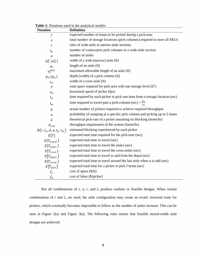
Table 1: Notations used in the analytical models

Notation Definition

𝐼 expected number of items to be picked during a pick-tour

𝑠 total number of storage locations (pick columns) required to store all SKUs

𝑟 ratio of wide-aisle to narrow-aisle sections

𝑙𝑤 number of consecutive pick columns in a wide-aisle section

𝑎 number of aisles

𝑎𝑤𝑤 (𝑎𝑤

𝑛 ) width of a wide (narrow) aisle (ft)

𝑎𝑙 length of an aisle (ft)

𝑎𝑙𝑚𝑎𝑥 maximum allowable length of an aisle (ft)

𝑝𝑑 (𝑝𝑤 ) depth (width) of a pick column (ft)

𝑐𝑤 width of a cross aisle (ft)

𝑆 total space required for pick area with one storage level (ft2)

𝑣ℎ horizontal speed of picker (fps)

𝑡𝑝 time required by each picker to pick one item from a storage location (sec)

𝑡𝑤 time required to travel past a pick-column (sec) = 𝑝𝑤

𝑣ℎ

𝑘 actual number of pickers required to achieve required throughput

𝑢 probability of stopping at a specific pick column and picking up to 5 times

𝜆 theoretical pick-rate of a picker assuming no blocking (items/hr)

𝛬𝑟𝑒𝑞 throughput requirement of the system (items/hr)

𝐵 𝑟, 𝑙𝑤 , 𝑘, 𝑢, 𝑡𝑝 : 𝑡𝑤 estimated blocking experienced by each picker

𝐸 𝑇 expected total time required for the pick-tour (sec)

𝐸 𝑇𝑡𝑟𝑎𝑣𝑒𝑙 expected total time to travel (sec)

𝐸 𝑇𝑎𝑖𝑠𝑙𝑒𝑠 expected total time to travel the aisles (sec)

𝐸 𝑇𝑐𝑟𝑜𝑠𝑠 expected total time to travel the cross-aisles (sec)

𝐸 𝑇𝑑𝑒𝑝𝑜𝑡 expected total time to travel to and from the depot (sec)

𝐸 𝑇𝑐𝑖𝑟𝑐𝑙𝑒 expected total time to travel around the last aisle when a is odd (sec)

𝐸 𝑇𝑝𝑖𝑐𝑘 expected total time for a picker to pick I items (sec)

𝐶𝑠 cost of space ($/ft)

𝐶𝑘 cost of labor ($/picker)

Not all combinations of s, a, r, and lw produce realistic or feasible designs. When certain

combinations of r and lw are used, the aisle configuration may create an erratic traversal route for

pickers, which eventually becomes impossible to follow as the number of aisles increase. This can be

seen in Figure 2(a) and Figure 3(a). The following rules ensure that feasible mixed-width aisle

designs are achieved:

9

Rule 1: If 𝑟 ≠ 1, then lw must be an integer multiple of 𝑠

𝑎.

Rule 2: If 𝑟 = 1, then lw may be an integer multiple or even factor of 𝑠

𝑎.

Rule 1 ensures that sections of wide aisles and subsequent sections of narrow aisles must be whole

aisles when the aisle configuration is not composed of 50% wide aisles and 50% narrow aisles (i.e.,

𝑟 ≠ 1). This can be visualized in Figure 2, which illustrates both feasible and infeasible systems

when r = 3 ≠ 1. According to Rule 1, lw must then be a multiple of s/a = 32/4 = 8, which is not the

case in Figure 2(a). As a result, the layout of the picking area progressively worsens as the number of

aisles increases until the picker’s path is ultimately obstructed. In Figure 2(b), where lw = 8, the travel

path is well-defined and unobstructed for pickers to easily traverse through the picking area.

?

(a) Infeasible System (lw = 6 ≠ sa )

(b) Feasible System (lw = 8 = sa )

Figure 2: Illustration of Rule 1, where s = 32, a = 4, and r = 3

Rule 2 allows for mixed-widths within an aisle only when r = 1; i.e. the configuration is 50% wide

aisle and 50% narrow aisles. Figure 3 illustrates both feasible and infeasible systems when r = 1.

According to Rule 2, lw should be an integer multiple or even factor of s/a = 40/4 = 10. In Figure 3(a),

lw = 6 ≠ factor of 10 and so the layout of the picking area progressively worsens as the number of

aisles increases until the picker’s path is blocked. In Figure 3(b), lw = 2 = factor of 10, resulting in a

clear travel path which is easily traveled by the picker.

10

?

?

(a) Infeasible System (lw = 6)

(b) Feasible System (lw = 2; even factor of 𝑠 𝑎 )

Figure 3: Illustration of Rule 2, where s = 40, a = 4, and r = 1

The above two rules provide a quick way to identify feasible designs and serve as inputs to the

analytical models presented next.

11

4. Analytical Space Model

The analytical space model we develop in this section can be used for both single-width and

mixed-width aisle configurations. Figure 4 illustrates a mixed-width aisle configuration along with

the parameters used in our space calculation. An expression to determine the unused space, which

results as pick-columns need to be offset in mixed-width aisles, is presented later in this section.

D

Unused

space

al

w

wa n

wa

cw

pw

pd

½ pd Figure 4: Mixed-width aisle configuration (lw < s/a)

The total space (S) required for a single-width system (e.g., pure narrow or wide) is the sum

of the space requirements for aisles, racks, and cross-aisles. The simplest approach to calculating the

total space is to define the system’s length and depth, and calculate the picking area as the product of

these two dimensions. The elements that compose the system’s length include rack depth (pd) and

12

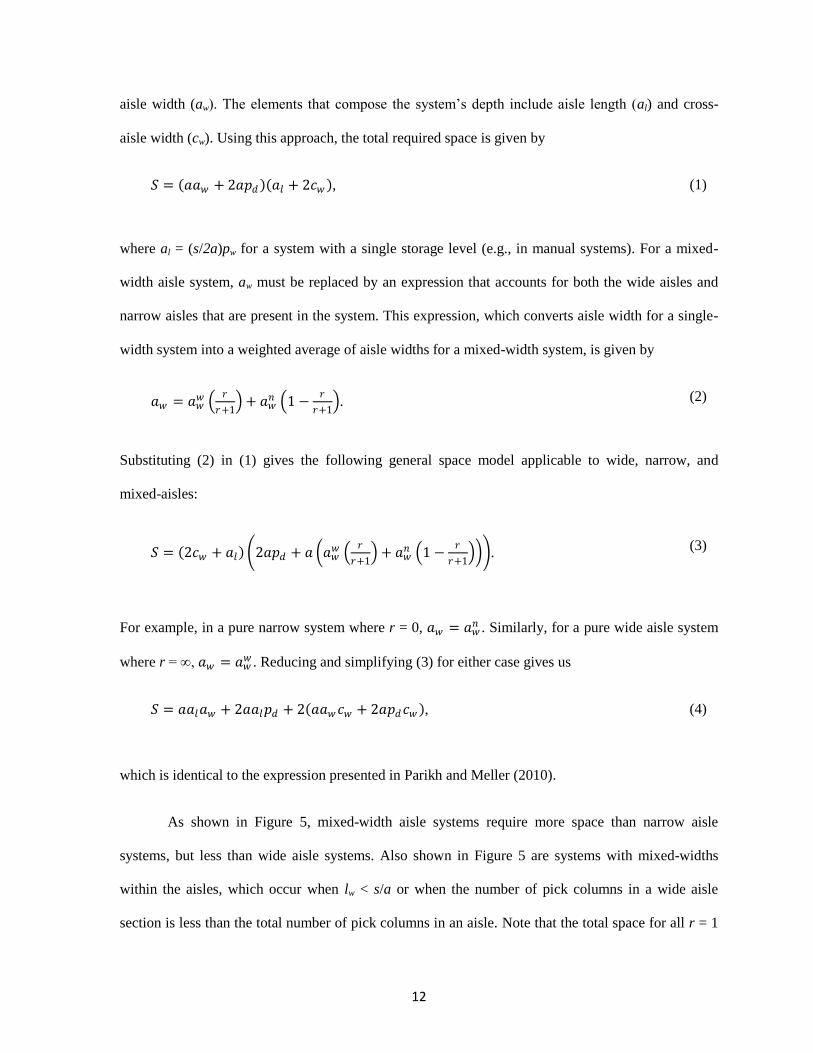
aisle width (aw). The elements that compose the system’s depth include aisle length (al) and cross-

aisle width (cw). Using this approach, the total required space is given by

𝑆 = 𝑎𝑎𝑤 + 2𝑎𝑝𝑑 𝑎𝑙 + 2𝑐𝑤 , (1)

where al = (s/2a)pw for a system with a single storage level (e.g., in manual systems). For a mixed-

width aisle system, aw must be replaced by an expression that accounts for both the wide aisles and

narrow aisles that are present in the system. This expression, which converts aisle width for a single-

width system into a weighted average of aisle widths for a mixed-width system, is given by

𝑎𝑤 = 𝑎𝑤𝑤

𝑟

𝑟+1 + 𝑎𝑤

𝑛 1 −𝑟

𝑟+1 . (2)

Substituting (2) in (1) gives the following general space model applicable to wide, narrow, and

mixed-aisles:

𝑆 = 2𝑐𝑤 + 𝑎𝑙 2𝑎𝑝𝑑 + 𝑎 𝑎𝑤𝑤

𝑟

𝑟+1 + 𝑎𝑤

𝑛 1 −𝑟

𝑟+1 .

(3)

For example, in a pure narrow system where r = 0, 𝑎𝑤 = 𝑎𝑤𝑛 . Similarly, for a pure wide aisle system

where r = ∞, 𝑎𝑤 = 𝑎𝑤𝑤 . Reducing and simplifying (3) for either case gives us

𝑆 = 𝑎𝑎𝑙𝑎𝑤 + 2𝑎𝑎𝑙𝑝𝑑 + 2 𝑎𝑎𝑤𝑐𝑤 + 2𝑎𝑝𝑑𝑐𝑤 , (4)

which is identical to the expression presented in Parikh and Meller (2010).

As shown in Figure 5, mixed-width aisle systems require more space than narrow aisle

systems, but less than wide aisle systems. Also shown in Figure 5 are systems with mixed-widths

within the aisles, which occur when lw < s/a or when the number of pick columns in a wide aisle

section is less than the total number of pick columns in an aisle. Note that the total space for all r = 1

13

mixed-width (lw < s/a) aisle systems is identical regardless of the value of lw. As seen in (3), space is

impacted by r and is independent of lw, with the following exception: mixed-widths (lw < s/a) result in

offset racks, and offset racks increase the length of the picking area by half a pick column depth, pd

(see Figure 4). Due to offset racks, the space required for system with r = 1 and mixed-widths

(lw < s/a) is larger than mixed-width systems with whole aisles (lw = s/a).

r = 0

r = 0.33

r = 1

r = 3

r

r = 1

(a) System representation

(b) System space comparison (s = 1,000, a = 20)

Figure 5: Mixed-width aisle systems and comparisons

Modifying (3) to account for offset racks in systems with mixed-width (lw < s/a) aisles, as shown in

Figure 4, gives us

𝑆 = 2𝑐𝑤 + 𝑠

2𝑎 𝑝𝑤 2𝑎𝑝𝑑 + 𝑎 𝑎𝑤

𝑤 𝑟

𝑟+1 + 𝑎𝑤

𝑛 1 −𝑟

𝑟+1 + 0.5𝛼𝑝𝑑 ,

(5)

where 𝛼 is a binary parameter that may be expressed as

𝛼 = 1, if 𝑙𝑤 < 𝑠

𝑎 ,

0, if 𝑙𝑤 ≥ 𝑠𝑎 .

40000

42000

44000

46000

48000

50000

52000

54000

56000

58000

60000

0 5 10 15 20

Sp

ace,

S (f

t2)

r

∞1/31 3 4

*

lw < s/a

14

Offsetting the racks, however, results space that is unused by racks or aisles. This concept of

unused space is unique to mixed-width (lw < s/a) aisle systems and is explored in the next section.

4.1. Unused Space

Unused space occurs in systems with mixed-width (lw < s/a) aisles and is found behind the

narrow section pick columns on the first and last aisle. This was illustrated in Figure 4, which showed

a system where s = 40, a = 4, r = 1, and lw = 2.

Unused space is the product of half the pick column depth, 𝑝𝑑 2 , the pick column width, pw,

and half the number of pick columns in an aisle, 𝑠 2𝑎 (Figure 4). When the number of aisles in a

system is odd and the number of pick columns on each side of an aisle are odd, the number of offset

pick columns that create unused space is one less than half the number of pick columns in an aisle. To

account for this, a binary parameter is used to subtract a “half pick column” from the equation. The

unused space for a mixed-width aisle system (with lw < s/a) can be calculated as

𝑆𝑢𝑛𝑢𝑠𝑒𝑑 = 𝑠

4𝑎− 0.5𝛽 𝑝𝑤𝑝𝑑 , (6)

where 𝛽 is a binary parameter that may be expressed as

𝛽 = 1, 𝑖𝑓 𝑎 is odd and 𝑠 2𝑎 is odd,

0, otherwise.

Since unused space only appears in the first and last aisle, it appears that for an r = 1 system, the most

unused space would be seen in layouts with a low number of aisles, and unused space would then

decrease as the total number of aisles increases. This leads us to the following theorem.

15

Theorem 1: The percentage of unused space for an r = 1 system converges to 0 as the number of

aisles approaches infinity.

Proof: The percentage of unused space for an r = 1 system is given by dividing equation (6) by the

total system space, S, and then multiplying by 100. We then take the limit of this modified equation,

as the number of aisles approaches infinity, as follows:

lim𝑎→∞

% 𝑆𝑢𝑛𝑢𝑠𝑒𝑑 = lim𝑎→∞

𝑠

4𝑎− 0.5𝛽 𝑝𝑤𝑝𝑑

𝑆× 100

≈ lim𝑎→∞

𝑠

4𝑎 𝑆= 0. ∎

The above fact is experimentally supported in Figure 6.

(a) Total space

(b) Unused space

Figure 6: Space comparison (r = 1, lw = 2)

Figure 6(a) shows the relationship between the number of aisles in a system and the total amount of

space required for a mixed-width system, where r = 1 and lw = 2. Notice the slight dip in the required

space for a < 10 aisles. Initially, as the number of aisles increases, the total required space decreases.

This is because the reduction in aisle length leads to a substantial decrease in the overall depth of the

0

10

20

30

40

50

60

70

0 10 20 30 40 50

Sp

ace,

S(1

00

0ft

2)

Number of aisles, a

s = 200

s = 400

s = 600

s = 800

s = 1000

0

1

2

3

4

5

6

200 400 600 800 1000

Un

use

d S

pac

e, f

t2

Total Pick-Columns, S

a = 1

a = 2

a = 4a = 5

a = 10a = 20a = 100

16

system as compared to the increase in aisle length that is attributed to the addition of aisles. As the

number of aisles increase, the reduction in system depth due to the reduction in aisle length becomes

minimal in comparison to the addition in length due to the additional aisles. Figure 6(b) indicates the

corresponding percentage of unused space, which tends to 0 as the number of aisles increases.

Having developed the analytical space model, we now focus on estimating the total amount

of time each picker spends traversing the picking area in a single pick tour.

17

5. Throughput Model

The number of pickers (k) required to satisfy the required throughput for a system (req) is

based on both the throughput of each picker as well as the blocking experienced by each picker. The

throughput generated by each picker, assuming that no blocking or idle time is experienced, is

referred to here as the theoretical pick rate () and is given by

𝜆 =3600𝐼

𝐸 𝑇 items/hr. (7)

The expected total time required is the sum of the expected total travel time and the expected time to

pick I items.

𝐸 𝑇 = 𝐸 𝑇𝑡𝑟𝑎𝑣𝑒𝑙 + 𝐸 𝑇𝑝𝑖𝑐𝑘 , where 𝐸 𝑇𝑝𝑖𝑐𝑘 = 𝐼𝑡𝑝 . (8)

The estimated travel time, 𝐸 𝑇𝑡𝑟𝑎𝑣𝑒𝑙 , associated with the pick tour is based on the travel path

followed by a picker through the aisles. The travel path is broken into four parts as follows: (i) travel

through the aisles, (ii) travel through the cross-aisles, (iii) travel to and from the depot, and (iv) time

to circle back toward the depot when the system has an odd number of aisles. For a manual system

with randomized storage policy and traversal routing, 𝐸 𝑇𝑡𝑟𝑎𝑣𝑒𝑙 can be estimated through

expressions (9) - (13), which generalize the expressions presented in Parikh and Meller (2010). The

binary parameter 𝛾, expressed as

18

𝛾 = 1, if number of aisles 𝑎 is odd0, otherwise

is used in the total time calculation to ensure that E[Tcircle] is included only when the number of aisles

is odd. Total travel time is thus expressed as

𝐸 𝑇𝑡𝑟𝑎𝑣𝑒𝑙 = 𝐸 𝑇𝑎𝑖𝑠𝑙𝑒𝑠 + 𝐸 𝑇𝑐𝑟𝑜𝑠𝑠 + 𝐸 𝑇𝑑𝑒𝑝𝑜𝑡 + 𝛾𝐸 𝑇𝑐𝑖𝑟𝑐𝑙𝑒 . (9)

We estimate E[Taisles] and E[Tcross] based on the number of aisles (a), the length of an aisle

(al), the cross-aisle width (cw), and the walking speed of the picker (vh); similar to Parikh and Meller

(2010). That is,

𝐸 𝑇𝑎𝑖𝑠𝑙𝑒𝑠 =𝑎𝑙𝑎

𝜈ℎ and (10)

𝐸 𝑇𝑐𝑟𝑜𝑠𝑠 =𝑐𝑤 𝑎 + 1

𝜈ℎ . (11)

The travel time to and from the depot is based on the number of aisles (a), the depth of a pick column

(pd), the single aisle width (aw), and the walking speed of the picker (vh) which is similar to Parikh

and Meller (2010). Substituting (2) for aw to account for mixed-width aisles gives

𝐸 𝑇𝑑𝑒𝑝𝑜𝑡 = 2 𝑎𝑤

𝑤 𝑟

𝑟 + 1 + 𝑎𝑤𝑛 1 −

𝑟𝑟 + 1 𝑎 − 1 + 2𝑝𝑑 𝑎 − 1

𝜈ℎ . (12)

When picking systems have an odd number of aisles, pickers exit the last aisle on the

opposite side than the depot is located, thus requiring them to return to the depot via circling around

19

the last aisle. The additional travel time required to circle around the last aisle is captured by E[Tcircle]

and is given by

𝐸 𝑇𝑐𝑖𝑟𝑐𝑙𝑒 =𝑎𝑙 + 2 𝑎𝑤

𝑤 𝑟

𝑟 + 1 + 𝑎𝑤𝑛 1 −

𝑟𝑟 + 1 + 2𝑝𝑑 + 𝑐𝑤

𝜈ℎ ,

(13)

where (2) is substituted for aw to account for mixed-width aisles.

Figure 7 illustrates that the expected total travel time required for a pick-tour increases as r

increases. We had earlier indicated that as r increases the total required space increases (see Figure

5(b)). Intuitively, both these observations make sense. Recall that r = 0 for pure narrow systems and

r=∞ for pure wide systems. As r increases, the system increases in size, thus increasing the amount of

time to travel through the system. Expression (7) indicates that the theoretical pick rate is inversely

proportional to the total travel time, as shown in Figure 7, and so as r increases, decreases. Based on

total system space and travel time, Figure 5 and Figure 7, maximum benefits can be realized when

r<5.

Figure 7: The effect of r on E[T] and (s = 1,000, a = 20)

It is worth noting that picker productivity could be reduced due to blocking, which we discuss

next.

80.0

80.5

81.0

81.5

82.0

82.5

83.0

83.5

84.0

84.5

0.356

0.358

0.360

0.362

0.364

0.366

0.368

0.370

0.372

0.374

0 5 10 15 20

,it

ems/

ho

ur

E[T

] (h

r)

r

∞1/3 1 3 4

E[T]

20

5.1. Effect of Picker Blocking on Picker Throughput

A picker may experience one of two types of blocking: pick-column blocking and in-the-aisle

blocking. Pick-column blocking occurs when two or more pickers need to pick at the same location.

In-the-aisle blocking is only experienced in narrow aisles and occurs when one or more pickers are

unable to pass someone who is actively picking (Parikh and Meller, 2009). When a picker is blocked,

they experience idle time and as a result are less productive. Because blocking is prominent in high-

throughput systems, its productivity-reducing effect must be accounted for when calculating a

system’s actual throughput. We developed a generic simulation model that can simulate any of the

three aisle-widths, pure wide, pure narrow, and mixed, to estimate the average blocking experienced

by pickers.

Blocking for mixed-width aisle systems is dependent on five factors: the ratio of wide to

narrow sections (r), the number of consecutive pick columns in a wide section (lw), the number of

pickers in the system (k), the pick-density (u), and the pick time to walk time ratio (tp:tw). We refer the

reader to Parikh and Meller (2009) for the procedure to estimate u for the given expected number of

items picked during a pick tour (I) and the total number of pick columns for a system (s).

Our simulation model uses concepts similar to those previously researched on blocking where

the picking area was modeled as one circular aisle (Gue et al., 2006; Parikh and Meller, 2009). In the

simulation, pickers alternate between wide aisles and narrow aisles as defined by lw and r. Blocking

per picker was measured both in the narrow and wide aisle sections and represented as

𝐵 𝑟, 𝑙𝑤 , 𝑘, 𝑢, 𝑡𝑝 : 𝑡𝑤 .

21

Figure 8: Blocking for less than full aisle configurations (s = 400, a = 10, k = 50)

Figure 8 shows blocking curves for varying lw values for a system where s = 400, a = 10, and

k = 50. For this system, lw = 40 results in full aisles of a single width and all others result in mixed-

widths (𝑙𝑤 < 𝑠 𝑎 ) within an aisle. When lw = 2 (= 4), wide aisle sections are very small (Figure 1),

allowing pickers a very limited opportunity to pass before entering a narrow section. This limited

opportunity reduces the effect of passing in wide aisles and behaves more similar to a pure narrow

system, hence the higher blocking. This phenomenon is shown in Figure 8, where we see the highest

blocking for lw = 2, followed by lw = 4 and then lw = 10, 20, and 40. The largest lw values (lw = 40, 20,

and 10) show blocking curves which are virtually identical where the two smallest lw values (lw = 4

and 2) show significantly higher blocking. We interpret this to mean that the actual number of pickers

needed to meet a required throughput would be the same for lw = 40, 20, and 10 with potentially

higher numbers of pickers needed for lw = 4 and 2. We conclude from this that the lowest cost will

favor higher lw values for this system configuration.

Recall from Section 4 that all mixed-widths (lw < s/a) for a system have the same required

total space. Also recall that total space for mixed-width (lw < s/a) aisles is larger than the total system

4

6

8

10

12

14

16

18

20

22

24

26

28

0 0.1 0.2 0.3 0.4 0.5

% o

f T

ime

Eac

h P

ick

er i

s B

lock

ed

Pick Density = I/s

lw=2

lw=4

lw=10

lw=20

lw=40

lw = 2

lw = 4

lw = 10

lw = 20

lw = 40

22

space required for mixed-width (lw = s/a) aisles due to offset racks. If lw = 40, 20, and 10 all have the

same number of pickers, and lw = 40 has the smallest required system space, then we can conclude

that lw = 40 will have the lowest total system cost. Generalizing this for all system configurations, we

conclude that for systems where r = 1, whole aisle configurations, (lw = s/a) will always be the

optimum configuration (even though it might not be the optimum r value for the system).

Having determined that whole aisle configurations are optimal, we can develop the

optimization model for determining the aisle layout that minimizes the total system cost.

23

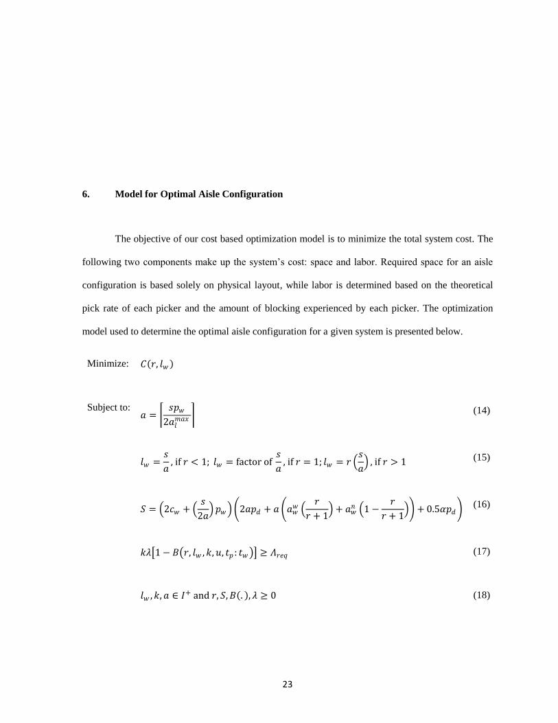
6. Model for Optimal Aisle Configuration

The objective of our cost based optimization model is to minimize the total system cost. The

following two components make up the system’s cost: space and labor. Required space for an aisle

configuration is based solely on physical layout, while labor is determined based on the theoretical

pick rate of each picker and the amount of blocking experienced by each picker. The optimization

model used to determine the optimal aisle configuration for a given system is presented below.

Minimize: 𝐶 𝑟, 𝑙𝑤

Subject to: 𝑎 =

𝑠𝑝𝑤

2𝑎𝑙𝑚𝑎𝑥 (14)

𝑙𝑤 =𝑠

𝑎, if 𝑟 < 1; 𝑙𝑤 = factor of

𝑠

𝑎, if 𝑟 = 1; 𝑙𝑤 = 𝑟

𝑠

𝑎 , if 𝑟 > 1

(15)

𝑆 = 2𝑐𝑤 +

𝑠

2𝑎 𝑝𝑤 2𝑎𝑝𝑑 + 𝑎 𝑎𝑤

𝑤 𝑟

𝑟 + 1 + 𝑎𝑤

𝑛 1 −𝑟

𝑟 + 1 + 0.5𝛼𝑝𝑑

(16)

𝑘𝜆 1 − 𝐵 𝑟, 𝑙𝑤 , 𝑘, 𝑢, 𝑡𝑝 : 𝑡𝑤 ≥ 𝛬𝑟𝑒𝑞 (17)

𝑙𝑤 , 𝑘, 𝑎 ∈ 𝐼+ and 𝑟, 𝑆, 𝐵 . , 𝜆 ≥ 0 (18)

24

The decision variables for this model are r and lw. The objective of the model is to minimize the total

system cost C(r, lw), which is the sum of the cost of space and the cost of labor. That is

𝐶 𝑟, 𝑙𝑤 = 𝑆𝐶𝑠 + 𝑘𝐶𝑘 .

Through (14) we ensure that the number of aisles in the system does not exceed the maximum

allowable length. Through (15) we ensure that optimal lw designs are considered by limiting lw to

whole aisle values. The total space required for a system is calculated in (16). Constraint (17)

guarantees that the required throughput for the system is met, where B(.) is determined using the

simulation model for estimating blocking discussed earlier. Constraints (18) indicate bounds on the

decision variables in the discussion.

To solve the optimization model presented above, we present a formal solution procedure to

determine the most cost-effect system layout. For all feasible r values, where 𝑎

𝑟+1 is a positive integer,

follow the steps below:

Step 1: Calculate the number of aisles in the picking area, using 𝑎 = 𝑠𝑝𝑤

2𝑎𝑙 , where 𝑎𝑙 ≤ 𝑎𝑙

𝑚𝑎𝑥 .

Step 2: Estimate the total travel time, 𝐸 𝑇 , using (8).

Step 3: Calculate the theoretical pick rate (𝜆) using (7).

Step 4: Calculate the theoretical number of pickers required from the theoretical pick rate where

𝑘𝑡ℎ𝑒𝑜 =𝛬𝑟𝑒𝑞

𝜆.

Step 5: Estimate the percentage of time each picker is blocked, 𝐵 𝑟, 𝑙𝑤 , 𝑘, 𝑢, 𝑡𝑝 : 𝑡𝑤 , using the

simulation model discussed earlier.

25

Step 6: Calculate the actual throughput, 𝛬𝑎𝑐𝑡 = 𝜆𝑘𝑡ℎ𝑒𝑜 1 − 𝐵 𝑟, 𝑙𝑤 , 𝑘, 𝑢, 𝑡𝑝 : 𝑡𝑤 . If 𝛬𝑎𝑐𝑡 < 𝛬𝑟𝑒𝑞 ,

then set the new theoretical number of pickers to 𝑘𝑡ℎ𝑒𝑜 = 𝑘𝑡ℎ𝑒𝑜 + 1 and repeat Steps 5 and 6

until 𝛬𝑎𝑐𝑡 ≥ 𝛬𝑟𝑒𝑞 .

Step 7: Calculate the total required space (𝑆) as defined by (16).

Step 8: Calculate total system cost (labor and space).

We now present results of our experiments to illustrate the use of our proposed analytical and

optimization models.

26

7. Experiment Design and Results

The optimization model presented earlier was used to determine the optimal aisle

configuration for specific system parameters. Table 2 lists the levels and values of all the parameters

used in our experiments. Approximately 810 experiments were conducted for a manual system with

randomized storage and traversal routing.

The total number of possible r values for a given number of aisles (a) is equal to a + 1.

However, for the sake of experimentation, we did not include any r values which did not result in a

definitive repeatable pattern without interruptions, where the first aisle width was opposite of the last

aisle width (i.e. unless pure widths, those beginning wide should have ended narrow). For example, a

repeatable pattern for a = 10 and r = 0.25 would be NNNNWNNNNW, while a non-repeatable

pattern for r = 1.5 would be NWWNWWNWWN. For s = 1,000, we evaluated 5 r values (3 where

applicable), which identified the quartiles and included pure narrow (r = 0) and wide (r = ∞). The

same r values were evaluated for s = 400 with the exception of a = 10. For a = 10 (s = 400) we

evaluated 7 values for r (i.e., 0, 0.1111, 0.25, 1, 4, 9, and ∞) with uninterrupted repeatable patterns.

The results are presented in the following tables. It is worth noting that our optimal solutions were

derived considering only repeatable patterns; non-repeatable patterns exist, but we did not consider

those in our search for the optimal aisle-width in this exploratory study.

27

Table 2: Parameter values used in experimentation

Parameter Levels Values Evaluated

I 1 30

s 2 400, 1,000

a 3 2, 10, 20

req 3 1,000, 2,500, 3,750 (items/hour)

CS 3 1, 10, 25 ($/ft2)

CK 3 20,000, 30,000, 50,000 (annual loaded $/picker)

r 5 0, 0.25, 1, 4, ∞

lw 1 2, 4, 10, 20,…, s/a for r ≤ 1 or r(s/a) for r > 1

Table 3 shows the parameter values generated for each evaluated r configuration for a system

where s = 400, a = 10, and = 2,500. These parameters include total system space, total estimated

time, the theoretical pick rate of each picker, the blocking experienced by each picker, and the total

number of pickers required to meet the required system throughput considering blocking.

Table 3: Parameter values for s = 400, a = 10, = 2,500 system

r lw S

(ft2)

E[T]

(sec)

(items /hr) B(.) k

N 0 18,000 714.4 151.2 12.60% 19

0.25 40 19,200 719.8 150.0 11.06% 19

1 40 21,000 727.9 148.4 9.29% 19

4 160 22,800 736.0 146.7 3.76% 18

W 400 24,000 741.4 145.7 0.56% 18

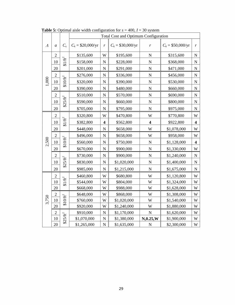
Table 4 shows a detailed cost comparison for each evaluated r configuration for a system

where s = 400, a = 10, and = 2,500. Where optimal, mixed-width aisles showed cost savings of

$1,200 to $48,000 over pure wide aisles. This translated into a 0.1% to 3.8% cost savings

improvement in comparison to pure wide systems with the same system parameters. These cost

savings could be classified as low to moderate. We speculate that mixed-width aisles might be more

suitable for a class based storage policy where higher demand items would be stored in wide aisle

28

sections and lower demand items would be stored in narrow aisle sections; this is discussed further in

Section 8. Mixed-width aisle configurations were optimal in systems where s = 400 and 1,000 for

both 2,500 and 3,750 throughputs. For all other combinations, pure narrow or pure wide

configurations were optimal. In many cases, multiple r values required the same number of pickers to

meet the required throughput. In these situations, the r value with the least amount of space was

always optimum. Table 5 and Table 6 show the optimal aisle configuration as well as the total system

cost for s = 400 and 1,000 systems respectively. Table 7 shows the space cost sensitivity of the

optimal aisle width configuration for an s = 1,000 system.

Table 4: Detailed cost comparison for s = 400, a = 10, = 2,500 system

R Space Cost

(x1,000)

Ck = $20,000 / yr Ck = $30,000 / yr Ck = $50,000 / yr

Labor Cost

(x1,000) Total Cost

(x1,000)

Labor Cost

(x1,000) Total Cost

(x1,000)

Labor Cost

(x1,000) Total Cost

(x1,000)

N

Cs =

$1/f

t2 $18 $380 $398 $570 $588 $950 $968

0.25 $19 $380 $399 $570 $589 $950 $969

1 $21 $380 $401 $570 $591 $950 $971

4 $23 $360 $383 $540 $563 $900 $923

W $24 $360 $384 $540 $564 $900 $924

N

Cs =

$10/f

t2 $180 $380 $560 $570 $750 $950 $1,130

0.25 $192 $380 $572 $570 $762 $950 $1,142

1 $210 $380 $590 $570 $780 $950 $1,160

4 $228 $360 $588 $540 $768 $900 $1,128

W $240 $360 $600 $540 $780 $900 $1,140

N

Cs =

$2

5/f

t2 $450 $380 $830 $570 $1,020 $950 $1,400

0.25 $480 $380 $860 $570 $1,050 $950 $1,430

1 $525 $380 $905 $570 $1,095 $950 $1,475

4 $570 $360 $930 $540 $1,110 $900 $1,470

W $600 $360 $960 $540 $1,140 $900 $1,500

29

Table 5: Optimal aisle width configuration for s = 400, I = 30 system

Total Cost and Optimum Configuration

a Cs Ck = $20,000/yr r Ck = $30,000/yr r Ck = $50,000/yr r 1

,00

0

2

$1

/ft2

$135,600 W $195,600 N $315,600 N

10 $158,000 N $228,000 N $368,000 N

20 $201,000 N $291,000 N $471,000 N

2

$1

0/f

t2 $276,000 N $336,000 N $456,000 N

10 $320,000 N $390,000 N $530,000 N

20 $390,000 N $480,000 N $660,000 N

2

$2

5/f

t2 $510,000 N $570,000 N $690,000 N

10 $590,000 N $660,000 N $800,000 N

20 $705,000 N $795,000 N $975,000 N

2,5

00

2

$1/f

t2 $320,800 W $470,800 W $770,800 W

10 $382,800 4 $562,800 4 $922,800 4

20 $448,000 N $658,000 W $1,078,000 W

2

$10/f

t2 $496,000 N $658,000 W $958,000 W

10 $560,000 N $750,000 N $1,128,000 4

20 $670,000 N $900,000 N $1,330,000 W

2

$25/f

t2 $730,000 N $900,000 N $1,240,000 N

10 $830,000 N $1,020,000 N $1,400,000 N

20 $985,000 N $1,215,000 N $1,675,000 N

3,7

50

2

$1/f

t2 $460,800 W $680,800 W $1,120,800 W

10 $544,000 W $804,000 W $1,324,000 W

20 $668,000 W $988,000 W $1,628,000 W

2

$10/f

t2 $648,000 W $868,000 W $1,308,000 W

10 $760,000 W $1,020,000 W $1,540,000 W

20 $920,000 W $1,240,000 W $1,880,000 W

2

$2

5/f

t2 $910,000 N $1,170,000 N $1,620,000 W

10 $1,070,000 N $1,380,000 N,0.25,W $1,900,000 W

20 $1,265,000 N $1,635,000 N $2,300,000 W

30

Table 6: Optimal aisle width configuration for s = 1,000, I = 30 system

Total Cost and Optimum Configuration

a Cs Ck = $20,000/yr r Ck = $30,000/yr r Ck = $50,000/yr r

1,0

00

2

$1

/ft2

$250,800 W $350,800 N $550,800 N

10 $280,500 N $400,500 N $640,500 N

20 $303,500 N $433,500 N $693,500 N

2

$1

0/f

t2 $601,000 N $711,000 N $931,000 N

10 $645,000 N $765,000 N $1,005,000 N

20 $695,000 N $825,000 N $1,085,000 N

2

$2

5/f

t2 $1,172,500 N $1,282,500 N $1,502,500 N

10 $1,252,500 N $1,372,500 N $1,612,500 N

20 $1,347,500 N $1,477,500 N $1,737,500 N

2,5

00

2

$1/f

t2 $550,800 W $800,800 W $1,300,800 W

10 $611,300 4 $891,300 4 $1,451,300 4

20 $690,750 1 $1,010,750 1 $1,650,750 1

2

$10/f

t2 $921,000 N $1,191,000 N $1,731,000 N

10 $985,000 N $1,275,000 N $1,855,000 N

20 $1,095,000 N $1,425,000 N $2,085,000 N

2

$25/f

t2 $1,492,500 N $1,762,500 N $2,302,500 N

10 $1,592,500 N $1,882,500 N $2,462,500 N

20 $1,747,500 N $2,077,500 N $2,737,500 N

3,7

50

2

$1/f

t2 $810,800 W $1,190,800 W $1,950,800 W

10 $894,000 W $1,314,000 W $2,154,000 W

20 $998,000 W $1,468,000 W $2,408,000 W

2

$10/f

t2 $1,201,000 N $1,611,000 N $2,408,000 W

10 $1,325,000 N $1,782,000 0.25 $2,640,000 W

20 $1,455,000 N $1,964,000 0.25 $2,930,000 W

2

$2

5/f

t2 $1,772,500 N $2,182,500 N $3,002,500 N

10 $1,932,500 N $2,392,500 N $3,312,500 N

20 $2,107,500 N $2,617,500 N $3,637,500 N

Table 7: Space cost sensitivity of optimal aisle width configuration for s = 1,000, = 2,500

Ck

=

$50,0

00/y

r Cs ($/ft2)

Aisles 1 2 3 4 5 6 7 8 9 10

2 W W W W W W W W N N

10 4 4 4 4 N N N N N N

20 1 1 1 1 1 1 N N N N

31

7.1. Managerial Insights

The above experimental study has helped us to derive managerial insights when configuring

aisles for OPSs. Wallace-Finney and Parikh (2011) found that system size (s), space cost (CS), and

required throughput (req) all had high degrees of influence, with conflicting directions of patterns

(wide to narrow vs. narrow to wide), on determining optimal aisle width. This suggests that the

optimum aisle configuration could change should the system size change due to aggregation or

disaggregation of storage locations, the throughput change due to growth or decline, or the cost of

land fluctuate due to inflation or recession. Decision makers should make sure their projections of

these values are strong in order to ensure a robust OPS design.

Our evaluation of the mixed-width aisle combinations, in conjunction with pure wide and

narrow under randomized storage and traversal routing, suggest the following:

Mixed-aisles are more desirable for system that require a larger number of storage locations

Mixed-aisles are more desirable for systems with a larger number of aisles

Mixed-aisles are least desirable at lower throughputs

Mixed-aisles are least desirable at higher space costs

Mixed-aisles are least desirable at lower labor costs

32

8. Summary and Future Research

The main contributions of this paper are the introduction of the mixed-width aisle layout as

an option to the OPS design process, and the corresponding analytical models for space and travel

time. Our derived models are general enough for evaluating pure narrow and wide aisles as well. The

travel time model was developed for a traversal routing policy which is best suited for systems that

employ a randomized storage policy.

To illustrate the use of these models, and analyze the potential benefits of a mixed-width aisle

system, we developed a cost-based optimization model to determine the optimal aisle configuration

for specific OPSs. The objective of this model was to minimize the total system cost which was

divided into two components, space and labor. Results indicated that while mixed-aisles are optimal

for certain systems with randomized storage and traversal routing, cost improvements over pure wide

aisle systems appear to be limited to 4% or less (up to $48,000) for systems where I = 30. These

savings may not be viewed as considerable; however the absolute savings in dollars appear to be

substantial for some of these configurations.

While further examination of varying values of I may produce higher cost savings, future

research into the use of mixed-width aisles should consider other OPSs such as semi-automated

systems that employ a person-onboard truck. Additional investigation into other storage policies is

required to fully understand the benefits of mixed-width aisle layouts. For example, an OPS with a

class based storage policy, wherein wide aisles are used for Class A items and narrow aisles for Class

33

B and C items, may result in additional benefits. The traversal routing policy may then be suboptimal

for class based storage. Consequently, an appropriate routing policy (such as modified traversal with

aisle skipping) would need to be used, for which a new travel-time model needs to be developed to

estimate the theoretical throughput of pickers. Furthermore, a new blocking model for estimating

average picker blocking would need to be developed. Doing so will allow the evaluation of the full

potential of mixed-width aisles for order picking in distribution centers.

34

References

De Koster, R., Le-Duc, T., and Roodbergen, K. J. (2007). Design and control of warehouse order

picking: a literature review. European Journal of Operational Research, 182 (2), 481-501.

Gu, J., Goetschalckx, M., and McGinnis, L. F. (2007). Research on warehouse operation: A

comprehensive review. European Journal of Operational Research, 177, 1-21.

Gue, K. R., and Meller, R. D. (2009). Aisle configurations for unit-load warehouses. IIE

Transactions, 41, 171-182.

Gue, K. R., Meller, R. D., and Skufca, J. D. (2006). The effects of pick density on order picking areas

with narrow aisles. IIE Transactions, 38 (10), 859-868.

Hong, S., Johnson, A. L., and Peters, B. A. (2010). Analysis of picker blocking in narrow-aisle batch

picking. Progress in Material Handling Research, 366-378.

Parikh, P. J., and Meller, R. D. (2010). A note on worker blocking in narrow-aisle order picking

systems when pick time is non-deterministic. IIE Transactions, 42 (6), 392-404.

Parikh, P. J., and Meller, R. D. (2010). A travel-time model for a person-onboard order picking

system. European Journal of Operational Research, 200, 385-394.

Parikh, P. J., and Meller, R. D. (2009). Estimating picker blocking in wide-aisle order picking

systems. IIE Transactions, 41, 232-246.

Petersen, C. G., and Aase, G. (2004). A comparison of picking, storage, and routing policies in

manual order picking. International Journal of Production Economics, 92, 11-19.

35

Roodbergen, K. J., and Vis, I. F. (2006). A model for warehouse layout. IIE Transactions, 38 (10),

799-811.

Roodbergen, K. J., Sharp, G. P., and Vis, I. F. (2008). Desiging the layout structure of manual order

picking areas in warehouses. IIE Transactions, 40 (11), 1032-1045.

Rouwenhorst, B., Reuter, B., Stockrahm, V., van Houtum, G. J., Mantel, R. J., and Zijm, W. H.

(2000). Warehouse design and control: Framework and literature review. European Journal

of Operational Research, 122, 515-533.

Skufca, J. D. (2005). k Workers in a Circular Warehouse: A Random Walk on a Circle, without

Passing. Society for Industrial and Applied Mathematics, 47 (2), 301-314.

Tompkins, J. A., White, J. A., Bozer, Y. A., and Tanchoco, J. A. (2003). Facilities Planning (3rd ed.).

New York, NY: Wiley.

Wallace-Finney, S. and Parikh, P. J. (2011). Determining the optimal aisle-width for order picking in

distribution centers. in review with European Journal of Operational Research.