an experimental study of a table-top doppler effect simulation · an experimental study of a...
TRANSCRIPT

Project Number: GSI - 0812
An Experimental Study of a Table-Top
Doppler Effect Simulation
A Major Qualifying Report submitted to
the faculty of Worcester Polytechnic Institute
in partial fulfillment of the requirements for
the Degree of Bachelor of Science
by
_____________________
Robert Lowry
_____________________
Caleb Teske
Keywords:
1. Experiment
2. Doppler
3. Simulation
_______________________________
Frederick L. Hutson, Co-Advisor
_______________________________
Germano S. Iannacchione, Co-Advisor

Table of Contents ACKNOWLEDGEMENTS ............................................................................................................................. I
ABSTRACT ................................................................................................................................................ II
EXECUTIVE SUMMARY ............................................................................................................................ III
1. INTRODUCTION .................................................................................................................................... 1
1.1 OVERVIEW OF PREVIOUS PROJECT................................................................................................................. 1
2. BACKGROUND ...................................................................................................................................... 7
2.1 GENERAL DOPPLER EFFECT ......................................................................................................................... 7 2.2 DOPPLER EFFECT FOR UNIFORM CIRCULAR MOTION ........................................................................................ 9 2.3 DERIVATION OF DOPPLER EFFECT FOR TILTED PLATFORM IN UNIFORM CIRCULAR MOTION ................................... 12
2.3.1 Special Cases .............................................................................................................................. 16 Special Case 1: ................................................................................................................................................. 16 Special Case 2: ................................................................................................................................................. 17 Special Case 3: ................................................................................................................................................. 18
3. METHODOLOGY ................................................................................................................................. 20
3. 1 DESIGN AND FABRICATION ....................................................................................................................... 23 3.1.1 The Motor Mount ....................................................................................................................... 23 3.1.2 The Motor Stand ........................................................................................................................ 27 3.1.3 The Arm ...................................................................................................................................... 29 3.1.4 Assembly .................................................................................................................................... 31 3.1.5 Other Design Considerations ...................................................................................................... 32
3.2 EXPERIMENTAL PROCEDURE ...................................................................................................................... 34 3.2.1 Laboratory Preparation .............................................................................................................. 34 3.2.2 Computer Preparation ............................................................................................................... 36
3.2.2.1 Configuring Spectrum Lab ................................................................................................................... 40 3.2.2.2 Configuring Logger Pro ........................................................................................................................ 44
3.2.3 Final Preparations ...................................................................................................................... 49 3.2.4 Acquisition of Doppler Data ....................................................................................................... 51 3.2.5 Acquisition of Supplemental Angular Velocity Data................................................................... 52
4. RESULTS ............................................................................................................................................. 53
4.1 DOPPLER TESTING RESULTS ....................................................................................................................... 54 4.2 ANGULAR VELOCITY TESTING RESULTS ........................................................................................................ 57
5. CONCLUSIONS .................................................................................................................................... 59
6. RECOMMENDATIONS ......................................................................................................................... 61
BIBLIOGRAPHY ....................................................................................................................................... 63
APPENDIX A – COMPLETE RESULTS OF DOPPLER TEST ........................................................................... 64

Table of Figures
FIGURE 1 - DOPPLER EXPERIMENT CONCEPT USING FRICTIONLESS CART ON TRACK...................................................... 2 FIGURE 2 - EXPERIMENTAL SETUP FOR DOPPLER EFFECT EXPERIMENT AS OF JANUARY 2009 .......................................... 3 FIGURE 3 – SAMPLE SPECTRUM LAB SCREENSHOT FROM PREVIOUS IQP GROUP.......................................................... 4 FIGURE 4 - CLOSE-UP OF HIGHEST BUZZER FREQUENCY FROM FIGURE 3 ................................................................... 5 FIGURE 5 - SCHEMATIC SIDE VIEW (A) AND TOP VIEW (B) OF EXPERIMENTAL SETUP .................................................... 9 FIGURE 6 – SCHEMATIC GEOMETRY FOR CALCULATING APPROACHING/RECEDING SPEEDS .......................................... 10 FIGURE 7 - SCHEMATIC SIDE VIEW OF EXPERIMENTAL SETUP USED FOR DERIVATION ................................................. 12 FIGURE 8 - SCHEMATIC OBLIQUE VIEW OF ROTATIONAL PLANE WITH ANGLE Θ INTRODUCED ....................................... 13 FIGURE 9 - SCHEMATIC SIDE VIEW OF EXPERIMENTAL SETUP SHOWING POSITION VECTORS L AND L₀ ............................ 14 FIGURE 10 - SIDE VIEW OF CONFIGURATION FOR SPECIAL CASE 1 .......................................................................... 16 FIGURE 11 - SIDE VIEW OF CONFIGURATION FOR SPECIAL CASE 2 .......................................................................... 17 FIGURE 12 - SIDE VIEW OF CONFIGURATION FOR SPECIAL CASE 3 .......................................................................... 18 FIGURE 13 - COMPLETED MOTOR MOUNT AND HOUSING ................................................................................... 24 FIGURE 14 - VIBRATION ISOLATION PAD USED FOR MOTOR MOUNT (LEFT) AND ALTERED VIBRATION ISOLATOR USED FOR
HOUSING (RIGHT) ............................................................................................................................. 25 FIGURE 15 - COMPLETED MOTOR STAND (BEFORE INSTALLING MOTOR MOUNT AND HOUSING) ................................. 29 FIGURE 16 - CLOSE-UP IMAGE OF SPINNING ARM .............................................................................................. 29 FIGURE 17 - COMPLETED SPINNING ARM ......................................................................................................... 31 FIGURE 18 - COMPLETED DOPPLER MACHINE WITH ARM ATTACHED ...................................................................... 32 FIGURE 20 - VOLUME ADJUSTMENT: STEP 1 ..................................................................................................... 36 FIGURE 21 - VOLUME ADJUSTMENT: STEP 2 ..................................................................................................... 37 FIGURE 22 - VOLUME ADJUSTMENT: STEP 3 ..................................................................................................... 38 FIGURE 23 - VOLUME ADJUSTMENT STEP 4 ...................................................................................................... 39 FIGURE 24 - SPECTRUM LAB INTERFACE ........................................................................................................... 40 FIGURE 25 - SPECTRUM LAB CONFIGURATION: PART 1 ....................................................................................... 41 FIGURE 26 - SPECTRUM LAB CONFIGURATION: STEP 2 ........................................................................................ 42 FIGURE 27 - SPECTRUM LAB DISPLAY FEATURES ................................................................................................ 43 FIGURE 28 - PROPER SETUP OF VERNIER LABPRO .............................................................................................. 44 FIGURE 29 - LOGGER PRO SOFTWARE CONFIGURATION: PART 1 ........................................................................... 45 FIGURE 30 - LOGGER PRO SOFTWARE CONFIGURATION PART 2 ............................................................................ 46 FIGURE 31 - LOGGER PRO CONFIGURATION: STEP 3 ........................................................................................... 47 FIGURE 32 - LOGGER PRO CONFIGURATION: STEP 4 ........................................................................................... 47 FIGURE 33 - LOGGER PRO CONFIGURATION: STEP 5 ........................................................................................... 48 FIGURE 34 - LOGGER PRO CONFIGURATION: STEP 6 ........................................................................................... 49 FIGURE 35 - SPECTRUM LAB SCREENSHOT OF BUZZER TEST .................................................................................. 50 FIGURE 36 - DOPPLER MACHINE TESTS AND CONFIGURATIONS ............................................................................. 51 FIGURE 37 - SCREENSHOT OF DATA RECORDED BY PREVIOUS GROUP ..................................................................... 55 FIGURE 38 - SCREENSHOT OF NEW DATA WITH DOPPLER MACHINE AT 0 DEGREE TILT ANGLE ..................................... 55 FIGURE 39 - SCREENSHOT OF NEW DATA WITH DOPPLER MACHINE AT 90 DEGREE TILT ANGLE ................................... 56 FIGURE 40 – RESULTS FROM TEST OF ANGULAR VELOCITY (REV/MIN) VS. BUZZER DISTANCE FROM CENTER OF ARM (CM)
WITH LINEAR TRENDLINE SHOWN .......................................................................................................... 58 FIGURE 41 - MICROPHONE 1/TEST 1 .............................................................................................................. 65 FIGURE 42 - MICROPHONE 2/TEST 1 .............................................................................................................. 66 FIGURE 43 - MICROPHONE 3/TEST 1 .............................................................................................................. 67 FIGURE 44 - MICROPHONE 1/TEST 2 .............................................................................................................. 68 FIGURE 45 - MICROPHONE 2/TEST 2 .............................................................................................................. 69 FIGURE 46 - MICROPHONE 3/TEST 2 .............................................................................................................. 70 FIGURE 47 - MICROPHONE 1/TEST 3 .............................................................................................................. 71 FIGURE 48 - MICROPHONE 2/TEST 3 .............................................................................................................. 72

FIGURE 49 - MICROPHONE 3/TEST 3 .............................................................................................................. 73 FIGURE 50 - MICROPHONE 1/TEST 4 .............................................................................................................. 74 FIGURE 51 - MICROPHONE 2/TEST 4 .............................................................................................................. 75 FIGURE 52 - MICROPHONE 3/TEST 4 .............................................................................................................. 76 FIGURE 53 - MICROPHONE 1/TEST 5 .............................................................................................................. 77 FIGURE 54 - MICROPHONE 2/TEST 5 .............................................................................................................. 78 FIGURE 55 - MICROPHONE 3/TEST 5 .............................................................................................................. 79 FIGURE 56 - MICROPHONE 1/TEST 6 .............................................................................................................. 80 FIGURE 57 - MICROPHONE 2/TEST 6 .............................................................................................................. 81 FIGURE 58 - MICROPHONE 3/TEST 6 .............................................................................................................. 82 FIGURE 59 - MICROPHONE 1/TEST 7 .............................................................................................................. 83 FIGURE 60 - MICROPHONE 2/TEST 7 .............................................................................................................. 84 FIGURE 61 - MICROPHONE 3/TEST 7 .............................................................................................................. 85 FIGURE 62 - MICROPHONE 1/TEST 8 .............................................................................................................. 86 FIGURE 63 - MICROPHONE 2/TEST 8 .............................................................................................................. 87 FIGURE 64 - MICROPHONE 3/TEST 8 .............................................................................................................. 88 FIGURE 65 - MICROPHONE 1/TEST 9 .............................................................................................................. 89 FIGURE 66 - MICROPHONE 2/TEST 9 .............................................................................................................. 90 FIGURE 67 - MICROPHONE 3/TEST 9 .............................................................................................................. 91 FIGURE 68 - MICROPHONE 1/TEST 10 ............................................................................................................ 92 FIGURE 69 - MICROPHONE 2/TEST 10 ............................................................................................................ 93 FIGURE 70 - MICROPHONE 3/TEST 10 ............................................................................................................ 94

I
Acknowledgements
During the course of the semester, we had a lot of problems to solve in a short
period of time. Thankfully, we had plenty of help from some various people on and off
campus and we would like to recognize those individuals properly.
First and foremost, we would like to thank our advisors, Fred Hutson and
Germano Iannacchione, for agreeing to take on an extra project with very short notice.
Our project team was given complete creative control over the design and manufacture of
the Doppler device and we received some great feedback from both advisors. Each had
their own ideas on ways we could improve our design and our testing methods. We both
enjoyed the laid back attitude and helpful insight of our advisors, as well as the timelines
that were provided early on in the semester. This kept us pointed in the right direction
and gave us a clear picture of what needed to be done and when. So thank you Fred and
Germano for helping us get the equipment we needed and putting up with our occasional
tardiness. You guys both made this project a lot of fun to work on.
Next we would like to thank Alexi Girgis, a long-time friend and graduate student
at WPI. Alexi was asked to help with the derivation of the Doppler effect for the case of
our device and to familiarize us with a vector graphics software program which allowed
us to draw some lovely figures for our derivation. We know that Alexi is extremely busy
and by no means obligated to help us so we would like to thank him very much for his
assistance.
We would also like to thank Christine Drew in the library. As usual, Christine was
great when we needed to find some relevant literature to look at. Her skill as a reference
librarian has saved us and probably many other students from hours of wandering around
hopelessly searching for the right book. She is a great person to know at this school and
we thank her for pointing us in the right directions.
Finally, we would like to thank everyone who had to listen to our buzzers while
we were testing for this project. We know that those buzzers are extremely annoying and
hard to listen to so if you happened to be subjected to that at any point during the
semester, thank you for your patience and understanding.

II
Abstract
This project was created as an extension of a previous IQP. The main goals were
to improve the design of an existing Doppler effect simulator and to be able to produce
reliable data such that this device can be used in the future for freshman laboratory
experiments. To meet these goals, the prototype model was completely redesigned to
improve stability, balance, and overall performance. With this new device, a battery of
systematic tests was carried out in which each controllable variable was isolated. The
results of these tests indicated that if more time is dedicated to completing a full analysis
of all data, this device could indeed be used as an exciting new way to demonstrate the
Doppler effect.

III
Executive Summary
The two most important questions that needed to be answered during the semester
were „What improvements can be made on a prototype model of a spinning Doppler
effect simulator?‟ and „Can repeatable data be generated, analyzed and synthesized for
the creation of an undergraduate laboratory experiment?‟
The motivation for this project was the continuance of a previous IQP from 2008.
This IQP group aimed to create a fun, interesting new experiment to demonstrate a well-
known physics concept and encouraged participation by keeping students engaged with
hands-on activities.
In fourteen weeks, the Doppler device was reconstructed with new materials, and
subjected to numerous tests under constantly changing conditions. Laboratory testing of
the new device during that period showed remarkable improvement in signal clarity and a
decrease in both vibration and audible noise inherent in the system. One factor that has a
potential to skew any test results is the reflection of sound waves of the solid walls and
floors of Olin Hall. Additionally, a set of Doppler equations that govern the situation
created in this experiment were derived from known Doppler cases.
Overall, testing demonstrated the fundamental soundness of the new Doppler
device. Work should continue steadily on this project to push it towards becoming a
usable laboratory experiment. When considering the advancement of this project, the
following actions are recommended:
Obtain an independent confirmation of equation derivations from a reputable source
Perform a full observational and mathematical analysis of Spectrum Lab results
Characterize the properties of the resonant and harmonic frequencies of the buzzer
when subjected to different configurations of the Doppler device
Make any additions or clarifications to the design or experimental procedure that could
not be made during the semester
Find a professor or someone that is a professional in the field of pedagogy and get some
expert suggestions on how to create clear and meaningful laboratory exercises using the
new Doppler device
1
1. Introduction
The Doppler effect experiment was developed as part of an IQP by the Physics
Production Corporation-a group of five WPI undergraduate students- and was presented
in January 2009. This group began to assemble a creative physics “toolbox” to help new
students grasp introductory physics concepts. The main goal of this IQP was to remodel
the freshmen level laboratories of the WPI Physics Department with these new “tools”
created for the physics “toolbox”. Another objective of this IQP was to create these tools
in a way that would be “innovative and exciting for the students” (Pydynkowski, Lessard,
Perry, McGinley, & Jones, 2009).
The tools created in Ongoing Advancement of the Physics Toolbox were intended
to lay a foundation that could be improved upon by future WPI project teams as well as
enhance the current state of the Physics Department. These tools are “far different than
anything that has been seen by freshman taking the introductory Physics classes thus far.”
(Pydynkowski, Lessard, Perry, McGinley, & Jones, 2009) The group, lead by Kyle
Pydynkowski, chose to design these experiments in a unique manner to “capture the
attention of the students who otherwise would not be interested in an introductory level
physics course.” (Pydynkowski, Lessard, Perry, McGinley, & Jones, 2009)
1.1 Overview of previous project
Kyle Pydynkowski and Konrad Perry were responsible for creating Physics
laboratories that could be used in any of the freshman Physics courses. Pydynkowski was
in charge of designing the device that would be used to carry out such experiments. The
goal of creating a lab such as the Doppler experiment was to present a well-known
concept in a new and interesting way and to encourage student attendance and
participation. This particular experiment was intended to engage all of the students
present for the lab session. The topic of the lab should also complement the lectures and
existing curriculum of the professors that teach the courses. In their report, Pydynkowski
and Perry state that “Every student should have an equal amount of work to do so that all
the students have an opportunity to learn.” (Pydynkowski, Lessard, Perry, McGinley, &
Jones, 2009)

2
The original concept for the Doppler lab involved using a frictionless cart on a
track. The cart would have a string attached to one end and hanging mass attached to the
end of the string. A pulley would be used to redirect the mass and use gravity to move the
cart along the track. A microphone would also be attached to the cart and was pointed in
the direction of a speaker and a position sensor at the opposite end of the track. A
program called Data Studio would then be used to emit a sound with a single waveform.
The configuration for this original idea is shown in Figure 1 below.
Figure 1 - Doppler Experiment Concept Using Frictionless Cart on Track
The microphone input could then be analyzed with a program called Spectrum
Lab. So the idea was to drop hanging mass and simultaneously release the cart while the
microphone records the sound coming from the speaker. Theoretically, students should
be able to visualize the Doppler effect and use the data to find the velocities and
frequencies of the speaker and microphone from the Doppler equations that are discussed
in Chapter 2.
However, this IQP group soon realized that in order to detect and record Doppler
effects, the cart would have had to be moving at a much faster speed than they
anticipated. Even though the group recommended this as a good way to show the Doppler
effect, the idea was adapted to be usable in the space provided in the WPI physics labs.
After realizing that the original design was impractical, the team decided to create
a lab that used some type of variation of the Doppler effect. After some brainstorming,

3
the group decided to create a spinning Doppler machine. The idea came from Astronomy
and is analogous to the rotation of a galaxy or a star. One can analyze the spectrum of
light emitted from a star in orbit, and just as easily analyze the spectrum of sound emitted
from a buzzer spinning around in a circle. The basic experimental setup for the Doppler
effect experiment can be seen in Figure 2 below.
Figure 2 - Experimental Setup for Doppler Effect experiment as of January 2009
An AC electric rotating motor is mounted in a square wooden box on top of a
piece of plywood. A long wooden arm is then mounted on the motor and fastened to the
motor mount with washers and screws. Buzzers were duct taped to each end of the arm
and connected to a 9V battery which was also duct taped to the arm several inches from
each from the buzzers. The motor was wired to an auto transformer or Variac which
allows the user to manually adjust the speed of the motor. A microphone is then placed
just outside the spinning radius of the arm and used to receive the sound being emitted by
the buzzers. The microphone is wired into a computer which runs a program called
Spectrum Lab. This software can be used for spectrum analysis of the incoming sound.
The spectrum can then be displayed in numerous ways depending on user preference. The
default display plots frequency on the horizontal axis and amplitude on the vertical axis.
A vertically-scrolling waterfall display can also be used to plot the resulting spectrum
4
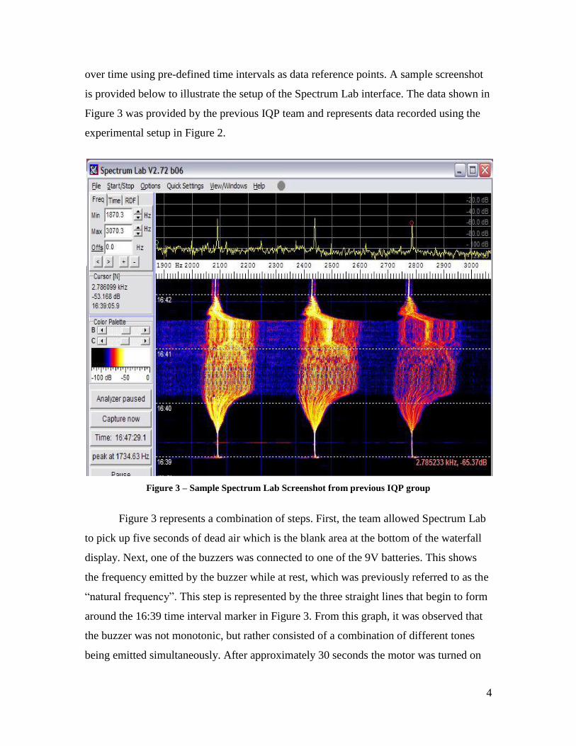
over time using pre-defined time intervals as data reference points. A sample screenshot
is provided below to illustrate the setup of the Spectrum Lab interface. The data shown in
Figure 3 was provided by the previous IQP team and represents data recorded using the
experimental setup in Figure 2.
Figure 3 – Sample Spectrum Lab Screenshot from previous IQP group
Figure 3 represents a combination of steps. First, the team allowed Spectrum Lab
to pick up five seconds of dead air which is the blank area at the bottom of the waterfall
display. Next, one of the buzzers was connected to one of the 9V batteries. This shows
the frequency emitted by the buzzer while at rest, which was previously referred to as the
“natural frequency”. This step is represented by the three straight lines that begin to form
around the 16:39 time interval marker in Figure 3. From this graph, it was observed that
the buzzer was not monotonic, but rather consisted of a combination of different tones
being emitted simultaneously. After approximately 30 seconds the motor was turned on

5
and slowly increased to an appropriately fast speed to record the Doppler effect. This can
be seen in Figure 3 above where the three frequencies begin to widen. Once the spectral
lines spread to their widest point, this indicates that the motor is at the maximum speed
for that time period. After less than one minute, the motor was slowly tilted toward the
microphone to a ninety degree angle. This can also be seen in Figure 3 around the 16:41
marker as the spectrum appears to intensify at a central frequency which looks much like
the spectrum for the buzzer at rest. This result is to be expected since the distance
between the buzzer and the microphone remains constant. At the top of Figure 3, around
the 16:43 marker, the motor was turned off and the rest frequency of the buzzer can be
seen again. Figure 4, below, isolated one of the buzzer frequencies and zoomed in to
show a close-up image of the same steps.
Figure 4 - Close-Up of Highest Buzzer Frequency from Figure 3

6
Although a proof of concept was established with this demonstration, the Doppler
effect experiment was never put into a laboratory format or tested by students due to lack
of time. However, the IQP team stated that “In the upcoming years of this ongoing IQP, a
lab could be made quite easily from the ideas and findings of this experiment.”
(Pydynkowski, Lessard, Perry, McGinley, & Jones, 2009) One recommendation the team
made for future project groups was that a louder buzzer would improve the system and
allow the microphone to detect the sound from farther away. Using a louder buzzer and
placing the microphone further away reduces noise in the system that can be created by
the sound of the motor running, as well as the wind noise created by the spinning arm.
Another recommendation was to find a buzzer with a single resonant frequency instead of
the multiple resonant frequencies that were shown in Figure 3. The harmonic frequencies
of the buzzer complicate the spectral analysis. A buzzer with a single resonant frequency
will show the exact same effects, but will be much cleaner and easier to analyze in
Spectrum Lab. The previous group also stated that there were some problems with
ordering the parts, so our group took that as a recommendation to get all the necessary
parts ordered soon enough to leave us sufficient time in the lab to perform tests. It is the
opinion of Pydynkowski and Perry that “Having this machine is a terrific starting point to
implement a laboratory experiment that has never been done before here at WPI. With
the use of the Doppler machine and the knowledge that was gained by this inaugural
Physics Production Company an educational laboratory experiment is within reach with
only a little more effort.” (Pydynkowski, Lessard, Perry, McGinley, & Jones, 2009)
7
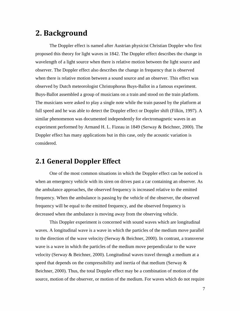
2. Background
The Doppler effect is named after Austrian physicist Christian Doppler who first
proposed this theory for light waves in 1842. The Doppler effect describes the change in
wavelength of a light source when there is relative motion between the light source and
observer. The Doppler effect also describes the change in frequency that is observed
when there is relative motion between a sound source and an observer. This effect was
observed by Dutch meteorologist Christophorus Buys-Ballot in a famous experiment.
Buys-Ballot assembled a group of musicians on a train and stood on the train platform.
The musicians were asked to play a single note while the train passed by the platform at
full speed and he was able to detect the Doppler effect or Doppler shift (Filkin, 1997). A
similar phenomenon was documented independently for electromagnetic waves in an
experiment performed by Armand H. L. Fizeau in 1849 (Serway & Beichner, 2000). The
Doppler effect has many applications but in this case, only the acoustic variation is
considered.
2.1 General Doppler Effect
One of the most common situations in which the Doppler effect can be noticed is
when an emergency vehicle with its siren on drives past a car containing an observer. As
the ambulance approaches, the observed frequency is increased relative to the emitted
frequency. When the ambulance is passing by the vehicle of the observer, the observed
frequency will be equal to the emitted frequency, and the observed frequency is
decreased when the ambulance is moving away from the observing vehicle.
This Doppler experiment is concerned with sound waves which are longitudinal
waves. A longitudinal wave is a wave in which the particles of the medium move parallel
to the direction of the wave velocity (Serway & Beichner, 2000). In contrast, a transverse
wave is a wave in which the particles of the medium move perpendicular to the wave
velocity (Serway & Beichner, 2000). Longitudinal waves travel through a medium at a
speed that depends on the compressibility and inertia of that medium (Serway &
Beichner, 2000). Thus, the total Doppler effect may be a combination of motion of the
source, motion of the observer, or motion of the medium. For waves which do not require

8
a medium, such as light, only the relative difference in velocity between the observer and
the source needs to be considered.
The most generalized form of the Doppler effect is given in terms of the resonant
frequency and the appropriate velocity components. The observed frequency f is related
to the emitted frequency of the source f₀ by the equation:
1 𝑓 = 𝑓₀ 𝑣 + 𝑣𝑟
𝑣 + 𝑣𝑠 ,
where ν is the velocity of waves in the medium, νs is the velocity of the source relative to
the medium and νr is the velocity of the receiver relative to the medium. In the case of a
stationary receiver (or microphone), the equation reduces to:
2 𝑓 = 𝑓₀ 𝑣
𝑣 + 𝑣𝑠 ,
where νs is positive when the source is moving away from the observer, and negative
when moving towards the observer. These equations assume that the source is directly
approaching or receding from the observer.

9
2.2 Doppler Effect for Uniform Circular Motion
A slightly more complex case of the Doppler effect involves a source in uniform
circular motion and a stationary receiver. During the literature review, an article was
discovered in a volume of Physics Teacher, a popular science journal. This article was
written by a group that conducted an experiment with a similar spinning Doppler
machine. In this experiment, a microphone was placed in the path of a spinning arm with
a buzzer attached. Images of the schematics for the experimental setup are shown below
in Figure 5.
Figure 5 - Schematic Side View (a) and Top View (b) of Experimental Setup
10
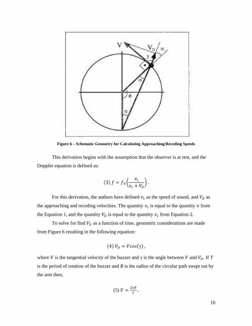
Figure 6 – Schematic Geometry for Calculating Approaching/Receding Speeds
This derivation begins with the assumption that the observer is at rest, and the
Doppler equation is defined as:
3 𝑓 = 𝑓₀ 𝑣𝑠
𝑣𝑠 + 𝑉𝐷 .
For this derivation, the authors have defined 𝑣𝑠 as the speed of sound, and 𝑉𝐷 as
the approaching and receding velocities. The quantity 𝑣𝑠 is equal to the quantity 𝑣 from
the Equation 1, and the quantity 𝑉𝐷 is equal to the quantity 𝑣𝑠 from Equation 2.
To solve for find 𝑉𝐷 as a function of time, geometric considerations are made
from Figure 6 resulting in the following equation:
4 𝑉𝐷 = 𝑉𝑐𝑜𝑠 γ ,
where 𝑉 is the tangential velocity of the buzzer and γ is the angle between 𝑉 and 𝑉𝐷. If T
is the period of rotation of the buzzer and R is the radius of the circular path swept out by
the arm then,
(5) 𝑉 =2𝜋𝑅
𝑇 ,

11
Substituting this value of 𝑉 will result into Equation 4 will result in a new
expression for 𝑉𝐷, which takes the form:
6 𝑉𝐷 =2𝜋𝑅cos(γ)
𝑇 .
From the angles in Figure 6, it is found that 𝜃 + 2𝛼 = 𝜋 and 𝛼 + 𝛾 = 𝜋/2.
Solving for 𝛾 gives the result 𝛾 = 𝜃/2. For a constant 𝑉,𝜃 = 2𝜋𝑡/𝑇, making 𝛾 = 𝜋𝑡/𝑇.
Substituting this back into Equation 6 gives:
7 𝑉𝐷 =2𝜋𝑅
𝑇cos
πt
𝑇 .
Substituting this expression back into Equation 3 will lead to the new form of the
Doppler equation:
8 𝑓 = 𝑓𝑜 𝑣𝑠
𝑣𝑠 +2𝜋𝑅𝑇 cos
πt𝑇
.
This Derivation was borrowed from The Doppler Effect of a Sound Source
Moving in a Circle (Saba & Antonio da S. Rosa, 2003). The next step is to generalize this
approach further by moving the microphone away from the path of the arm to a random
point in space and allowing the rotational plane to vary by 90 degrees. These subtle
changes in geometry make this problem much more complex.

12
2.3 Derivation of Doppler Effect for Tilted Platform in Uniform Circular Motion
Figure 7 - Schematic Side View of Experimental Setup Used for Derivation
Previous experiments involving the Doppler effect have focused on particular
geometries but do not account for the tilt angle of the device β. Here the observed
frequency of the Doppler shift is derived for a random value of β and a random
microphone position. The knowledge gained from the literature review provided the
necessary background information to attempt this derivation. First consider a rotated
coordinate system defined by the transformation,
9 𝐱 ′
𝐲 ′
𝐳 ′
= cos β 0 sin β
0 1 0−sin β 0 cos β
𝐱 𝐲𝐳 .
For this case, the 𝐲 unit vector does not change and only the 𝐱 ′and 𝐳 ′component
need to be considered,
(10) 𝐱 ′ = cos β 𝐱 + sinβ 𝐳 ,
11 𝐳 ′ = − sin β 𝐱 + cos β 𝐳 .

13
Figure 8 - Schematic Oblique View of Rotational Plane with Angle θ Introduced
The arm is rotating with scalar angular velocity about the 𝐳 ′axis.
12 ω =dθ
dt ,
such that the vector angular velocity is given by:
13 𝛚 = ω 𝐳 ′ = ω − sin β 𝐱 + cos β 𝐳 .
The vector location of the buzzer, with respect to the point of rotation, is given in
terms of the rotational position of the arm, θ, which is measured from the 𝐱 ′ axis.
14 𝒓 = R sin θ 𝐲 + R cosθ 𝐱 ′.
Substituting Equation 10 into Equation 14 leads to the result:
15 𝒓 = R sin θ 𝐲 + R cosθ 𝐱 cos β + 𝐳 sinβ .
This result is then simplified to:
16 𝒓 = 𝑅 cos θ cos β 𝐱 + sin θ 𝐲 + cosθ sin β 𝐳 .

14
Figure 9 - Schematic Side View of Experimental Setup Showing Position Vectors L and L₀
The relevant quantity to determine the Doppler shift is the component of the
buzzer velocity along the vector 𝐋, which runs from the microphone to the buzzer. This is
given as the following dot product:
17 VD = 𝐋 ∙ 𝐯 =𝐋 ∙ 𝐯
𝐋 ,
where
18 𝐋 =𝐋
𝐋 .
Already having defined the quantities 𝝎 and 𝒓, it is a simple matter to determine
the vector velocity of the buzzer:
19 𝐯 = 𝝎 × 𝒓 .
Taking the cross product results in the following expression for 𝐯:
20 𝐯 = 𝑅𝜔
𝐱 𝐲 𝐳 − sin β 0 cos βcos θ sin θ sin β cos θ
,
= 𝑅𝜔 – cos β sin θ 𝐱 + sin2 β cos θ + cos2 β cos θ 𝐲 − sin β sin θ 𝐳 ,

15
21 𝐯 = Rω − cos β sin θ 𝐱 + cos θ 𝐲 − sin β sin θ 𝐳 .
The vector 𝐋 is the sum of a vector 𝑳0, from the microphone to the center of the
arm,
22 𝐋0 = L 𝐱 + h − ℓ 𝐳 ,
and the vector location 𝒓 determined above, such that:
23 𝑳 = 𝑳0 + 𝒓.
Substituting Equations 16 and 22 into Equation 23 and simplifying gives the
following expression for 𝐋:
24 𝐋 = L + R cos β cos θ 𝐱 + R sin θ 𝐲 + h − ℓ + R sin β cos θ 𝐳 .
The magnitude of 𝐋 is then calculated as follows:
𝐋 2 = L2 + R2 cos2 β cos2 θ + 2LR cos β cos θ + R2 sin2 θ
+ h − ℓ 2 + R2 sin2 β cos2 θ + 2 h − ℓ R sin β cos θ ,
= L2 + R2 + h − ℓ 2 + 2R cos θ L cos β + h − ℓ sin β ,
25 𝐋 = L2 + R2 + h − ℓ 2 + 2R cos θ L cos β + h − ℓ sin β 1
2 .
The dot product in the expression for VD is then:
𝐋 ∙ 𝐯 = −Rω cos β sin θ L + R cos β cos θ + Rω cos θ R sin θ + −Rω sin β sin θ h − ℓ + R sin β cos θ ,
𝐋 ∙ 𝐯 = −LRω cos β sin θ − R2ω cos2 β sin θ cos θ + R2ω cos θ sin θ− Rω h − ℓ sin β sin θ − R2ω sin2 β sin θ cos θ ,
𝐋 ∙ 𝐯 = R2ω cos θ sin θ 1 − 1 − LRω cos β sin θ − Rω h − ℓ sin β sin θ ,
26 𝐋 ∙ 𝐯 = −Rω sin θ L cos β + h − ℓ sin β .
At last, a solution is reached and the final expression for VD is found to be:
27 VD =−Rω sin θ L cos β + h − ℓ sin β
L2 + R2 + h − ℓ 2 + 2R cos θ L cos β + h − ℓ sin β 1
2 .

16
It can be seen from Equation 27 that moving the microphone out of the path of the
arm and allowing the plane of rotation to be changed has resulted in a complex solution
for the approaching and receding velocities. This is to be expected when two extra
degrees of freedom are introduced to a system. Although the math seemed to work out
perfectly, the team needed a way to confirm the results.
2.3.1 Special Cases
Since no independent verification has been received regarding the validity of the
derived quantities from the previous section, three special cases were considered.
Checking the Doppler equations for these cases and comparing them with the expected
results should indicate whether or not the derivation makes sense. The three special cases
are configured as follows:
1) Doppler device spinning flat ( β = 0 ) with the plane of rotation at the same height as
the microphone ( h = ℓ ).
2) Doppler device spinning at 90 degrees ( β =π
2 ) with the point of rotation a distance R
above the microphone ( h = ℓ + R ).
3) Doppler device spinning at 90 degrees (β =π
2 ) with the point of rotation at the same
height as the microphone ( h − ℓ = 0).
Special Case 1:
Figure 10 - Side View of Configuration for Special Case 1

17
Substituting β = 0 and h = ℓ + R into Equation 27 and solving for vD yields:
vD,1 =−R ω sin θ L
L2 + R2 + 2LR cos θ 1
2 .
It is clear that vD,1 is zero for θ = 0, π both conceptually and from the expression
above.
The cases θ = ±π
2 result in the following form for vD,1 ±
π
2 :
vD,1 ±π
2 =
∓R ω L
L2 + R2 1
2 .
One can verify this result by using the following expressions for 𝐋 and 𝐯:
𝐋 = L 𝐱 ± R 𝐲 , 𝐯 = ∓ R ω 𝐱 , and directly computing vD,1.
vD,1 ±π
2 =
𝐋 ∙ 𝐯
𝐋 =
∓R ω L
L2 + R2 1
2 .
Special Case 2:
Figure 11 - Side View of Configuration for Special Case 2

18
Substituting β =π
2 and h = ℓ + R into Equation 27 and solving for vD yields:
vD,2 =−R2ω sin θ
L2 + 2R2 1 + cos θ 1
2 .
When θ = 0, π, at the top and bottom positions, it is clear that VD,2 = 0. The cases
θ = ± π2 result in the following form for vD,2 ±
π
2 :
vD,2 ±π
2 =
∓R2ω
L2 + 2R2 1
2 .
Again, one can verify this result by using the following expressions for 𝐋 and 𝐯:
𝐋 = L 𝐱 + R 𝐳 ± R 𝐲 , 𝐯 = ∓R ω 𝐳 ,
and directly computing vD,2, in the same manner as Special Case 1.
vD,2 ±π
2 =
𝐋 ∙ 𝐯
𝐋 =
∓ R2 ω 𝐲
L2 + 2R2 1
2
Special Case 3:
Figure 12 - Side View of Configuration for Special Case 3

19
Substituting β =π
2 and h − ℓ = 0 into Equation 27 and solving for vD yields:
vD,3 =−Rω Lsin θ cos
π2
0
L2 + R2 + h − ℓ 2 + 2R cos θ L cosπ2
0
12
= 0 .
It is clear, conceptually, that in this configuration, at all points of rotation, the
velocity of the buzzer is perpendicular to 𝐋.
Due to time constraints, an independent confirmation of this derivation is still
needed. However, these special cases were setup as a way to check the results of the
derivation. The equation was expected to reduce in a certain way for each case, and in
each case, the derived equation behaves as predicted, implying that these results make
sense.

20
3. Methodology
The purpose of this project was to improve upon the design of the old Doppler
effect machine created by five undergraduate students at WPI in 2008. This machine was
intended for use in a freshman-level laboratory experiment to simulate the acoustic
Doppler effect. Due to lack of time, and what must have certainly been a tight schedule,
the previous group created a rough model of a spinning Doppler machine, which was a
great starting point for future groups. However, since their model was indeed rough, this
project aimed to create a new device with the hope of making the system more reliable so
accurate data could be gathered. In order to create a reliable system, detailed research was
conducted to learn more about the components that make up this system. Once more
information was gained about the individual parts of the machine and how their
performance could affect Doppler simulation, the machine could be rebuilt and new data
could be collected. A literature search was also conducted to find out if any similar
experiments had been used elsewhere, and if so, what was done to assure the accuracy of
the data collection. A set of goals for the semester were created and listed below,
followed by the strategies employed by our team to solve this problem. Finally, a
description of the design considerations for each component of this machine is also
included.
Expectations/Goals for Semester:
Complete a full review of work done by previous project group
Perform a comprehensive literature review to learn more about the Doppler effect
and the different ways in which Doppler shifting can be observed
Research all components of the Doppler machine and analyze their effectiveness
Rebuild the spinning Doppler device created by the previous group
Test this new device under as many configurations as possible including: varying
motor speed, varying the radius of the buzzer from the center of the spinning arm,
and varying the angle at which the entire device is tilted
Reduce or eliminate all non-buzzer noises in the signal to allow for optimal data
collection

21
Gather reliable Doppler effect data using our rebuilt machine and Spectrum Lab
and interpret this data for laboratory use
Come up with a set of equations that describe the Doppler effect in several
different cases: general Doppler effect, circular Doppler effect, and a combination
of angled and circular Doppler effect
In order to accomplish these goals, there were several strategies that were
employed. Below is a list of the strategies used to accomplish the goals stated above. The
numbers below correspond to the numbers above in the list of expectations and goals.
Strategies for meeting Expectations/Goals:
Read the IQP provided to us by Fred Hutson and learn as much as possible about
the previous model of this machine to gain a better understanding of how
everything works together
The literature review was completed by speaking with Christine Drew in the
library. Christine helped the team locate a few documents that proved very useful.
Other literature in the form of Physics text books was obtained from Alexi Girgis
Information was obtained on the internet regarding the construction and
components of the old Doppler machine
After the parts were researched, several weeks were spent gathering materials and
assembling the new and improved Doppler machine
To test the machine, many hours needed to be spent acquiring data in the lab.
Since experiments are constantly going on during the semester, the team had to
work around the existing lab schedule
Noise will be eliminated by making a more stable machine with a balanced
spinning arm and a level base to secure the machine to the pedestals in the lab.
Replacing the old polytonic buzzer with a new monotonic buzzer will also help
reduce noise
A series of 10 tests was devised to gather a wide range of Doppler effect data.
These tests were intended to provide a complete data set and cover a variety of
possible experimental configurations

22
To derive the Doppler equations for a point in space away from an angled sound
source in uniform circular motion, a night was spent consulting with Physics
graduate student Alexi Girgis. New Doppler equations were derived based on an
old form of the equation
Creating lists of goals and strategies for accomplishing these goals helped to keep
the research focused. These lists also helped to motivate the design and testing processes.
This allowed group members to narrow down research efforts to obtain only relevant
material and waste as little time as possible in the search for applicable information.

23
3. 1 Design and Fabrication
The final device is made of several sections that together provide the adaptability
necessary for a critical laboratory experiment. The sections were constructed one at a
time and are essentially independent of each other. This allows for easy repair and
redesign of the sections.
The required features of the device included: easy placement on a table or lab
bench pedestal, one degree of freedom to vary the angle of rotation from 0 to 90 degrees
from vertical, and a variable buzzer radius. To achieve the desired features, three sections
were devised and constructed: the motor mount, the motor stand, and the arm. In this
section, a detailed description of the materials and design considerations for the Doppler
machine is provided.
3.1.1 The Motor Mount
The previous project had surrounded the motor on all sides with a wooden box
made from plywood, which in principle worked well. This box was reconstructed out of
1” x 5” pine, with a 4” square interior space. The bottom was left open, and the motor
was suspended from the top of the box and secured to plate made of Plexiglas. Plexiglas
was chosen for its ease of manufacturability and transparency. The motor came equipped
with #8-32 x 11/16” screws attached to the ends of the housing for easy mounting (see
Figure 13 on next page).

24
Figure 13 - Completed Motor Mount and Housing
The vibrations produced by the motor were heuristically determined to be a result
of the motor mount not absorbing, but amplifying vibration noise. In the previous project
the motor was held in place with metal straps which allowed for lateral vibration and
collision with the motor mount walls. The spinning arm for the project was not going to
be a precision device, and chances were that the center of mass would not be perfectly
on-axis. The motor mount needed to absorb as much of the vibration from the motor and
from the arm as possible. Pliable rubber pieces installed at various stages of the
construction provided a means for these vibrations to be absorbed. With built in
compliance the vibrations could be kept close to their sources and hopefully not
transmitted through the device, as this could cause the addition of unwanted audible
noises.
Rubber compliance was added in two places between the axel and the bottom of
the motor mount to remove noise. Vibration isolators, #8-32 stand-offs made of rubber
encased around a nut just above the head of a screw, provided a mounting mechanism
that at some point in its length had a cross section made entirely of rubber. This allowed
the motor to swing around inside the motor mount with its off-axis center of mass. This
concept was then applied to the entire motor mount box, where vibration pads were
added underneath the corners of the motor mount. This would allow any vibrations that

25
were transmitted through the last rubber isolators or produced by the cooling system to be
absorbed before they reached the motor stand. These pads were acquired from Grainger
Industrial Supply in Worcester. Below is a sample of the type of pads that were used to
absorb vibration.
Figure 14 - Vibration Isolation Pad Used for Motor Mount (Left) and altered Vibration Isolator Used
for Housing (Right)
Later in the design process many arms were experimented with, and it was found
that the motor was not going to spin at full speed with an arm long enough to have a large
range of radial variability for the buzzer. Since the motor was running under speed, it was
overcoming great resistance from the arm and produced heat. Heat was to be expected
but the high temperature shut off should not be reached during the course of a fifty
minute lab.
The arm with the most resistance was chosen to do a cooling test. The motor was
turned on until the high temperature limit was reached, and then allowed to cool down for
ten minutes. Each trial consisted of running from this warmed up state to the high
temperature limit. The Plexiglas had no holes for air, and the motor mount had three 3/8”
holes near the bottom. The vibration pads created an opening below the motor mount
walls, about 3/8” by 1 1/2” centered on each side. The run time was less than ten
minutes, which was not long enough for a proper auditory lab test to be performed.
To remedy this issue, computer fans were added to the sides of the motor mount
for increased cooling. A 6-Volt AC/DC adapter from Radio Shack was installed to

26
provide power for the computer fans. Originally, two fans were installed in an IN/OUT
configuration which blew air across the housing of the motor, perpendicular to the axel
and the cooling holes in the motor housing. This helped increase the runtime to fourteen
minutes, which was still inadequate. A third fan was added, and they were all configured
to blow out, thus drawing all air in through the bottom and out the sides. Run time did not
improve from here.
The original 1/15th
horse power (HP) motor spun at 3000 revolutions per minute
(rpm), but this was not the case with the arm attached. Since this speed was visually
estimated to be less than 500 rpm, there was a significant amount of heat from resistance.
A different motor with 1/40th
HP motor was installed with the same configuration. The
power output was less and the standard speed was 1550 rpm, so when forced to run at
near 500 rpm, this motor was under less stressful conditions. A time test was performed
with the same rigorous arm and manually aborted at 135 minutes, well longer than the
target length of fifty minutes. At this point the 1/15th
HP motor was retired.
The mounting needed to be adjusted for the smaller motor because of a different
standoff configuration. The larger motor had four screws evenly placed around the top,
while the smaller motor had only two. With only two screws, the rubber allowed the
motor to swing violently. The smaller motor had the same two screws in the same
position on the bottom of the motor, to which the remaining two vibration isolators were
added. A copy of the piece of Plexiglas which holds the top of the motor to the top
surface of the motor mount box was made for the bottom of the motor. The upper piece
was 5 1/2” square, but the lower piece needed to be approximately 3.9” square to fit
inside the box. This lower piece was attached firmly inside and this plate provided further
stabilization for the motor. However, the location of the plate cut off the air flow to the
fans. The cooling holes in the motor housing were drawn onto the bottom Plexiglas and a
near circle was removed so air could rush into the bottom of the motor or around the
bottom of the housing. The space between the vibration pads along the bottom of the
motor mount walls was heightened to about 5/8” to increase air flow. Cooling was again
verified to be fifty minutes and then canceled.
In order to accurately measure the rotation of the motor, a Vernier Rotary Motion
device was added to the side of the motor mount. Two plastic pulley wheels were

27
fashioned to belt the axle of the motor to the axle of the sensor. The pulley ratio was
measured with dial calipers to be 1.4401, with the sensor spinning faster than the device.
The results of tests done with this sensor can be seen in Section 4.2.
The new motor mount reduced the noise and vibration when tested with the
original arm, and the device ran much smoother than the previous model. Also, at this
point a run time of longer than one lab period was achieved, which was a big step
forward.
3.1.2 The Motor Stand
The motor mount could sit on a table and function properly, but needed to be
affixed to something that would allow it to be secured to a lab pedestal and tilted to up to
90 degrees. A piece of 3/4” seven lap plywood was chosen to do the job. The plywood
would need to hinge and be able to be stopped anywhere during its motion. The
construction was designed from the lab bench up.
A rectangle of plywood formed the base from which everything else would grow.
Thinner plywood was laminated to the sides to create a pocket under the machine that
was 7/8” tall and 10 1/2” wide. Aluminum strips were screwed into the bottom edges of
the pocked to create a lip which would slip over 5mm lip of the lab bench pedestal. One
half of a vibration isolation square was added to the four corners of the aluminum so that
the device could also be used while sitting on a table. Two handles were added at the
extremes of the plywood, centered vertically, so that the device could be picked up and
slid left to right onto the pedestal. Three #10-24 thumb screws were installed into bottom
mounted T-nuts capped with push nuts covered with 1/10” adhesive backed felt as
mounting screws to pin the device to the pedestal. Each hole was topped with a #10 flat
washer attached with superglue around the hole. This allowed for a simple and quick way
to securely mount a flat plywood sandbox from which a second movable plain rotate.
A square with 11” sides was cut from the same plywood stock and used for the
motor mount to be fixed to. This square was centered and then left justified on the
rectangular stand. To allow for wires to pass underneath, two strips of the same plywood
were cut about 2” wide and fixed to stand where the top and bottom most reaches of the

28
square would be. These acted as a foundation to elevate the square. A notch was cut in
the front strip to allow the wires to pass through the middle and out to make it to the top
of the square and to the motor mount. These strips were covered with 1/10” rubber gasket
material and secured with masking tape. This runner would help to quiet any potential
noise between the square and the stand. The two were connected with a pair of 2 1/2”
hinges indented 1/2” from the sides. A handle was added to the end grain of the top edge
of the square for easy angular adjustment.
The motion of the square was created by affixing a pair of lid slides to the left and
right of the forward section of the square. They were placed so that the maximum reach
of the arm was marginally past 90 degrees. The screws that allow the device to slide were
replaced with thumb screws for easy adjustment. To assist with the measurement of the
tilt angle, a protractor was created from 1/8” Plexiglas and mounted to the side of the
forward foundation strip so that the bottom of the square was a reference line and the
pivot point was along the axis of the hinges. A store-bought protractor was used to mark
multiples of five degrees from 0 to 90. The square now had the capability to move
through the desired range of motion and be measured.
The terminals were exposed for easy working, but were dangerously exposed.
Previously the terminals were covered with duct tape. In the new design, the electrical
panel was positioned in the upper right hand corner of the stand and surrounded with
Plexiglas for safety. The 6V adapter and the 110V motor cable were plugged in under the
Plexiglas and the wires were run under the square and out through the notch and up to the
top of the square. A picture of the finished motor stand without the motor mount attached
is shown in Figure 15 on the next page.
29
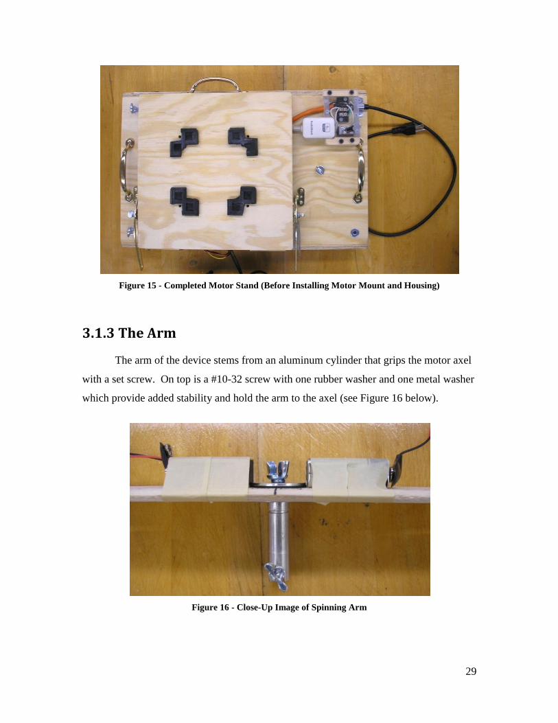
Figure 15 - Completed Motor Stand (Before Installing Motor Mount and Housing)
3.1.3 The Arm
The arm of the device stems from an aluminum cylinder that grips the motor axel
with a set screw. On top is a #10-32 screw with one rubber washer and one metal washer
which provide added stability and hold the arm to the axel (see Figure 16 below).
Figure 16 - Close-Up Image of Spinning Arm

30
Originally the arm was made of 1/4” x 2” Balsa, but a Plexiglas disk idea came up
to challenge it. By removing the incident edge of the spinning blade, a disk would
hopefully remove unwanted air resistance. A 10” x 1/4” Plexiglas disk was fabricated,
but the speeds at which it spun were dangerous and concerning. The main difference with
the Plexiglas over the Balsa was the density. The high density of the Plexiglas coupled
with the high angular speed meant that a small displacement lead to wild vibrations. The
Balsa was so light that if the center of mass of the arm was not exactly on-axis then the
resulting vibrations were not as dramatic. To make the disk feasible, its design, as well as
the load placed on top of it, would have to be perfectly balanced, and the effort of
keeping the center of mass that precise with moving wires and buzzers was not practical.
The disk was eventually abandoned in favor of the blade shaped arm.
The blade went through several iterations before a final width and length were
selected. When an arm with a 6” radius was tested, the speed was similar to the
dangerous disks, so an arm of sufficient length and mass was necessary. If the arm was
too long, it could cause the motor to overheat. The ideal length was found to be around
30” and the arm was cut accordingly. Assuming the device is mounted to a lab pedestal,
this allows just enough room to tilt the device to 90 degrees and spin the arm without the
hitting the table. The edges of the blade were tapered at a slight angle as a way to reduce
air resistance.
Once the shape of the arm was chosen, a buzzer was mounted near each end of
the arm to serve as the sound source for Doppler simulation. The buzzers were purchased
from http://www.digikey.com/ and have a resonant frequency of 4500 ± 500 Hz. To add
another degree of freedom to the system, the idea arose to allow the buzzers to slide up
and down the length of the arm. For this purpose, thin grooves were cut along the center
line of the arm on either side of the center of rotation. The buzzers were fixed to small
rectangular sliding pieces of Plexiglas that transport the buzzers along the arm length.
Two thumb screws were installed on each buzzer slide so the position of the buzzers may
be fixed at a desired location. The arm was then marked with units of inches on one side
and centimeters on the other side for easy measurement. Two 9V batteries were taped
around the center of rotation and wire leads were installed to connect the batteries to the
buzzers. Figure 17 on the next page shows the completed arm.
31
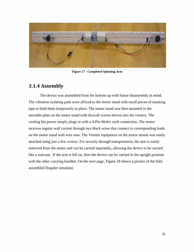
Figure 17 - Completed Spinning Arm
3.1.4 Assembly
The device was assembled from the bottom up with future disassembly in mind.
The vibration isolating pads were affixed to the motor stand with small pieces of masking
tape to hold them temporarily in place. The motor stand was then mounted to the
movable plate on the motor stand with drywall screws driven into the corners. The
cooling fan power simply plugs in with a 4-Pin Molex style connection. The motor
receives regular wall current through two black wires that connect to corresponding leads
on the motor stand with wire nuts. The Vernier equipment on the motor mount was easily
attached using just a few screws. For security through transportation, the arm is easily
removed from the motor and can be carried separately, allowing the device to be carried
like a suitcase. If the arm is left on, then the device can be carried in the upright position
with the other carrying handles. On the next page, Figure 18 shows a picture of the fully
assembled Doppler simulator.

32
Figure 18 - Completed Doppler Machine with Arm Attached
3.1.5 Other Design Considerations
During the design portion of the project, many different ideas were investigated in
hopes of creating the ideal lab instrument. Some of these ideas worked to our advantage,
while some ideas failed completely. Two particularly interesting ideas arose concerning
alternate methods of powering the buzzers.
The first idea involved sliding contacts, which would allow the batteries to be
taken off the arm, reducing weight and air resistance. This concept was similar in theory
to how a bumper car is powered. The fender washer on the bottom of the arm was
isolated from the other metallic components of the hardware that connects the arm to the
axel of the motor. Two contacts were produced from the 9V battery and were run up to
the top of the motor mount. The common was allowed to rub against the aluminum shaft,
while the hot was allowed to rub against the fender washer. In this configuration, the
motor and most of the hardware was considered at 0V, while the fender washer on the

33
bottom was charged with 9V. A wire was attached under the top common washer and the
bottom hot washer, and the lower wire was moved to the top through a small hole. These
wires were attached to the same terminal device that connected to the 9V batteries,
essentially producing a battery on the arm that was not actually there. The wires that
would rub against the washers were 18 gage steel wire, bent in the direction of motion.
The sliding contact idea was sound, and several consumer extension cord storage devices
use the concept to make a variable length extension cord. In practice it worked well, and
after some adjustment the connection was continuous and unwavering. The major
problem was that the grinding of the metal against metal was producing too much noise,
and had become louder than the motor and the air resistance of the blade. This idea could
still be refined to reduce noise with the benefit of lower wind resistance and higher blade
velocity.
The other idea that came up was suggested by two WPI graduate students. These
gentlemen referred us to the PowerStream Power Supplies and Chargers website at
http://www.powerstream.com/. This company sells batteries that can be molded to
different shapes to meet different conditions. These batteries are about the size of a stick
of gum and weigh much less than a 9V battery. However, research indicated that one of
these batteries would only power a buzzer for 5-15 minutes depending on the model. So
although these batteries are rechargeable, the frequency at which recharging would be
necessary is not convenient. Therefore, this idea was abandoned until battery technology
advances to a point where it would be more practical in this application.
This device is sturdy and well built, and many considerations were made to
guarantee its effectiveness. However, due to time constraints, the design of the device
was eventually frozen to move forward with data collection. Therefore, anyone that
becomes involved with this project in the future should always be thinking of ways to
improve upon the current design.

34
3.2 Experimental Procedure
Preparing the laboratory and setting up the computer to acquire data for this
experiment requires the users to prepare the laboratory space and the computers before
beginning any actual testing.
Before this experiment can be used as part of a physics course at WPI, the
behavior of the Doppler device had to be characterized in all of its possible
configurations. In order to do this, a systematic battery of tests was devised that would
isolate all variables in the Doppler equation. Observing the behavior of the device in this
manner allowed the team to see how each individual variable affects the observed sound
output, as recorded by the microphones.
3.2.1 Laboratory Preparation
In order to gather the best possible data, some basic preparation needs to be done
in the lab. Of the three labs that were used throughout the semester, the best results for
this experiment were recorded in OH117. It is recommended that this room be used for
any future applications of this project as it is larger than the labs on the second floor. The
larger room reduces noise that can be caused by the reflection of sound waves off the
walls, as well as the ceiling and floor.
The first thing that should be done is to slide the Doppler device onto a pedestal at
one of the lab stations and fasten the base securely to the surface by using the three
thumb screws that have been built into the base. This will assure that the machine is flat
against the top of the pedestal and provide stability to help eliminate vibrations when the
motor is running. Then plug the machine in to an outlet. Each of these pedestals has its
own power supply so there should be no problem finding an available plug to use. Also,
connect the cooling fans to the power supply using the 4-pin connector.
Once the Doppler device is setup, a microphone must be connected to the
computer, or multiple computers if desired, and positioned appropriately to receive the
incoming sound from the buzzers. The majority of data taken in OH117 was gathered
with three microphones, each farther away from the source than the next. The pedestals
on the lab stations are ideal for placing the microphones as they raise the microphones

35
high enough off the table to be approximately level with the Doppler machine when not
tilted. One microphone was placed closer to the machine and raised up on boxes to make
it level with the others. A photo of the laboratory setup with the three microphones was
taken and is shown belowto demonstrate one possible configuration for this experiment.
Figure 19 - Table-Top View of Microphone Positioning Used for Data Collection (from Left to Right:
Microphone 1, 2, 3)
The microphones were numbered one through three, with number one being
closest to the source and number three farthest away. In Figure 11, from left to right,
microphones one, two, and three can be seen in testing configuration. Of course, this is
only one possible arrangement of microphones. Microphones may be placed around the
room wherever there is a computer station, which means data can be collected from
anywhere in the lab. Raising the microphones off the table-top improves signal clarity
since the amplitude of the buzzer is weaker when measured below the arm. Make sure
that the microphone is not set to “Mute”. There is a small switch on the front of the
microphone boom that allows the user to turn the microphone off and on. The up position

36
is “Mute”, and the down position is “On”. To further improve clarity in the signal, try to
clear as much material off the lab tables as possible and rearrange the computers so that
nothing is in the path from the microphone to the buzzer.
3.2.2 Computer Preparation
Once the microphones are in position and the Doppler machine is properly
secured and powered, the next portion of preparation for this experiment is to make sure
the computer or computers being used for testing are properly configured. This is a very
important procedure and it is crucial to assure that all computers operate with the same
settings.
Begin by logging on to the computers that will be used. After logging in, first
make sure the sound settings on the computer are properly adjusted. To change the sound
settings double click the speaker icon in the bottom-right hand corner of the desktop as
demonstrated in Figure 20 below.
Figure 20 - Volume Adjustment: Step 1

37
If the master volume is muted in the “Volume Control” window, uncheck the
“Mute All” Box. Most of the computers will default to maximum volume but
occasionally the master volume is muted for some reason, so it is wise to check before
continuing. From the “Volume Control” window, select “Options” and then select
“Properties” as shown in the Figure 21 below.
Figure 21 - Volume Adjustment: Step 2

38
In the Properties window under “Adjust Volume For”, select “Recording” and
then click “OK” to close the window (refer to Figure 22).
Figure 22 - Volume Adjustment: Step 3

39
This brings up the “Recording Control” window which should now display the
volume level for the microphone. Make sure this is set at maximum volume and close the
window (see Figure 23).
Figure 23 - Volume Adjustment Step 4
Performing this check prior to testing will assure that the volume of the incoming
signal is audible. If the volume level of the microphone is too low, it is possible that the
Spectrum Lab software will be unable to detect the signal.

40
3.2.2.1 Configuring Spectrum Lab
Once the equipment is setup and the computer is adjusted, the user can open
Spectrum Lab. The user should now be looking at a blank Spectrum Lab window that
looks like this:
Figure 24 - Spectrum Lab Interface

41
Spectrum Lab is software that acts as an audio analyzer, data recorder, and much
more. The first thing users should do is select the “Quick Settings” drop-down menu and
click “Restore all „Factory‟ Settings” (see Figure 25 below).
Figure 25 - Spectrum Lab Configuration: Part 1
Then click “Yes” in the pop-up box that follows. This will return you to the main
window of Spectrum Lab. Occasionally, if Spectrum Lab runs for too long, the results
become unreliable and restoring the default settings each time before testing should
eliminate this problem, as well as ensure that all computers have the same configuration.

42
The frequency range is displayed across the horizontal axis while the amplitude is
shown on the vertical axis. This range can be adjusted by entering the desired minimum
and maximum values into the text-boxes in the top-left corner of Spectrum Lab (refer to
Figure 26 below).
Figure 26 - Spectrum Lab Configuration: Step 2
When entering a value, wait a few seconds for the software to redraw the screen
before you move the cursor out of that box, otherwise, the program will just revert back
to the last value that was entered. The frequency of the buzzers used for testing can be
easily detected between 4000 and 5000 Hertz. Closer resolution can also be achieved to
view results in more detail.
Over time, the grey area will begin to fill in with the recorded sound spectrum.
The time is marked every 60 seconds by a dashed line horizontally across the screen.
When a sound is received by the microphone, it is displayed in the frequency versus
amplitude graph at the top of the screen, while the time-based results are recorded and
shown in the Waterfall display directly below. An image of these features is provided in
Figure 27 on the next page.

43
During the course of the testing for this project, it was noted that many computers
did not have Spectrum Lab installed. When a location is selected in which to perform this
experiment, it is recommended that most current version of Spectrum Lab be installed on
all computers in that lab. This will allow for students at any station to record their own
data sets. It should also be noted that Spectrum Lab is not currently compatible with
Windows Vista. If the school should happen to upgrade the lab computers before this
issue is resolved, an alternative program would need to be found.
Figure 27 - Spectrum Lab Display Features

44
3.2.2.2 Configuring Logger Pro
This section of the experiment is optional, but should be implemented if time
permits. During the final three weeks of the semester, an innovative feature was added on
to the Doppler device which allows users to measure the angular velocity of the spinning
arm. Although this contraption is not constructed from the highest quality parts, the
accuracy of these results indicates that the new Doppler device is precise enough to
generate reliable angular velocity data. Using the Logger Pro software, users can observe
the change in angular velocity as the buzzers are moved to different positions along the
arm.
If it is decided that appropriate time can be allotted to making these
measurements, continue reading through this section for a step-by-step tutorial on how to
configure the Logger Pro software for rotary motion. If this portion on the experiment is
not going to be used, skip to the next section entitled Other Considerations.
Begin by plugging the Vernier LabPro into an outlet and the plug the Rotary
Motion Device into the port labeled DIG/SONIC 1 on the Vernier LabPro (Figure 28,
below).
Figure 28 - Proper Setup of Vernier LabPro
45
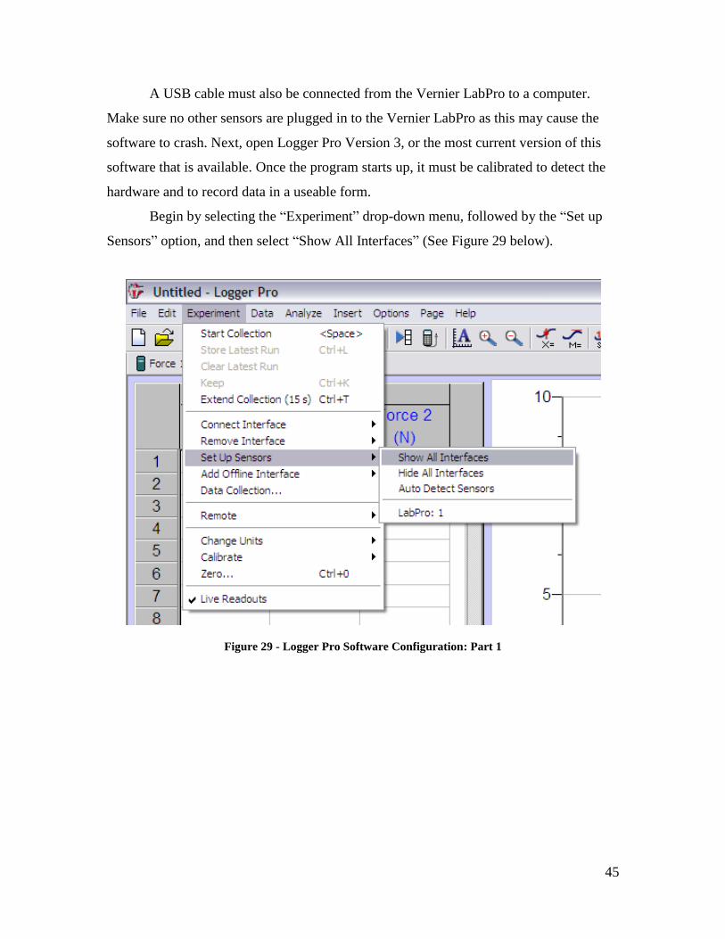
A USB cable must also be connected from the Vernier LabPro to a computer.
Make sure no other sensors are plugged in to the Vernier LabPro as this may cause the
software to crash. Next, open Logger Pro Version 3, or the most current version of this
software that is available. Once the program starts up, it must be calibrated to detect the
hardware and to record data in a useable form.
Begin by selecting the “Experiment” drop-down menu, followed by the “Set up
Sensors” option, and then select “Show All Interfaces” (See Figure 29 below).
Figure 29 - Logger Pro Software Configuration: Part 1

46
Next, click on the box labeled “DIG/SONIC1”, select “Choose Sensor...”, and
then pick “Rotary Motion” from the list of sensors. This step is shown in Figure 30
below.
Figure 30 - Logger Pro Software Configuration Part 2
Once the computer has detected the Rotary Motion sensor, the program will
return you to the “Show All Interfaces” window again. The next step is to select the
desired units. To do this, again click the box labeled “DIG/SONIC1” and select “rev” to
change the units to revolutions (See Figure 31 at top of next page).
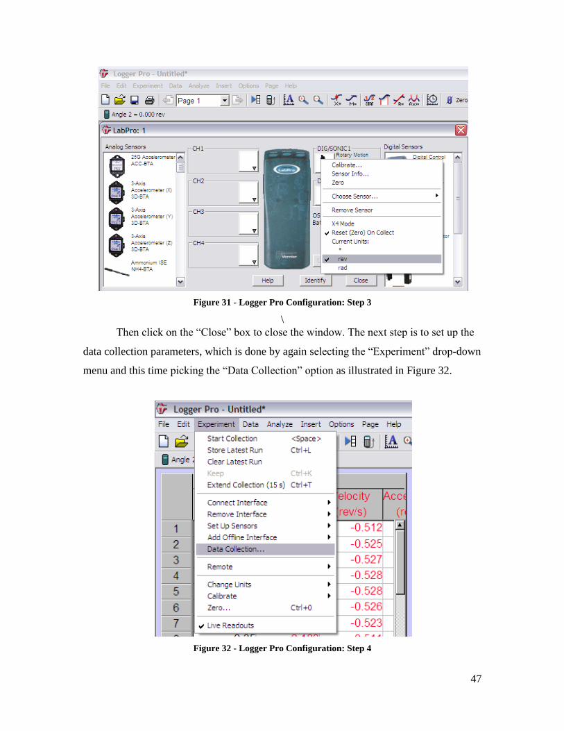
47
Figure 31 - Logger Pro Configuration: Step 3
\
Then click on the “Close” box to close the window. The next step is to set up the
data collection parameters, which is done by again selecting the “Experiment” drop-down
menu and this time picking the “Data Collection” option as illustrated in Figure 32.
Figure 32 - Logger Pro Configuration: Step 4

48
From the “Data Collection” menu, users can adjust the Sampling Rate and the
desired duration of the test. Enter a value of 100 in the box labeled “samples/second”,
and enter the desired time in the box labeled “Length”. These quantities are highlighted
in Figure 33 below.
Figure 33 - Logger Pro Configuration: Step 5
Selecting a Sampling Rate higher than 100 samples per second may cause the
computer to freeze and cost valuable lab time, especially if Spectrum Lab is also running
in the background. Click the “Done” box once these values are selected. This will bring
the user back to the original Logger Pro window. At this point, the Doppler machine
should be switched on and allowed to reach maximum velocity before collecting data.
Once the maximum velocity is achieved, click the green button labeled “Collect”, and the
computer will record the data (refer to Figure 34 at top of next page).

49
Figure 34 - Logger Pro Configuration: Step 6
Occasionally the computers will lag and 30 seconds of data collection will take 60
seconds of real time, but aside from taking slightly longer than expected, the results will
generally finish with no problems. Once the collection is finished, the data sets will be
listed in columns on the left-hand side of the window and graphs of the angular velocity
and angular displacement will be displayed to the right of the data sets. Rotary motion
data may be gathered in conjunction with the Doppler data while the buzzer is operating,
or alternatively, the data can be gathered separately while the buzzer is silent.
3.2.3 Final Preparations
The final task before recording any data is to warm up the buzzer. Only one of the
two mounted buzzers needs to be turned on to collect data. The other is essentially a
counterweight, and must be set at the same distance from the center of the arm as the
other buzzer. Failure to do this will cause instability in the rotation of the arm. The buzzer
that is to be used for testing needs to be warmed up for approximately two to three
minutes or until the frequency becomes approximately constant over time. To activate the
buzzer, connect the wire leads to the 9V battery on the arm. As the buzzer begins to emit
sound, users can observe as the resonant frequency or “steady state” is approached. This
state will be represented by a straight vertical line in the Waterfall display of Spectrum
Lab. Before the buzzer reaches this steady frequency, it tends to deviate slowly so be sure
to allow proper warm up time for the buzzer. A buzzer that is properly warmed up should
look similar to the sample image shown in Figure 35 on the next page.

50
Figure 35 - Spectrum Lab Screenshot of Buzzer Test
Anything color that can be seen that is not a vertical line in this image is noise is
the system. This happens to be a screenshot of the data from the microphone that was
closest to the buzzer. Due to the high pitch of this buzzer, extra noise is inevitable from
this close range, however reliable results can still be captured.
As a final caveat to users of this machine, it is highly recommended that you wear
some sort of ear protection when participating in this experiment. The frequency of the
tone emitted by this buzzer is very high pitched and absolutely obnoxious to listen to for
any extended period of time. The Physics Department is advised to provide ear plugs to
any students involved in this procedure. The Mechanical Engineering Department has
spare ear plugs that could probably be acquired for use in Olin Hall. A high quality set of
headphones would also suffice. Also, bear in mind that the buzzers can be heard
throughout the hallways of the building, so do everyone a favor and keep the doors shut
while the buzzers are operating.

51
3.2.4 Acquisition of Doppler Data
The laboratory and computers should now be completely setup and Doppler data
can now be gathered from the machine. For testing purposes, 10 different tests were
performed and for each test three microphones were used in the configuration shown
previously in Figure 19. Each test combined different configurations of buzzer positions
on the arm, angular velocity, and degree of tilt of the device. Additionally, the use of
three microphones allowed the group to record the spectrum as a function of distance
from the sound source for each of the 10 tests. By using three microphones at different
positions, the number of tests is essentially reduced from 30 to 10, as multiple data sets
can be collected simultaneously. The test configurations are listed and described in the
chart below.
Test
Number
Doppler Machine Status Buzzer Position
(cm)
Angle of Tilt
(degrees)
1 NOT SPINNING
(Buzzer Test Only)
34cm 90
2 SPINNING 12cm 0
3 SPINNING 12cm 45
4 SPINNING 12cm 90
5 SPINNING 25cm 0
6 SPINNING 25cm 45
7 SPINNING 25cm 90
8 SPINNING 34cm 0
9 SPINNING 34cm 45
10 SPINNING 34cm 90
Figure 36 - Doppler Machine Tests and Configurations
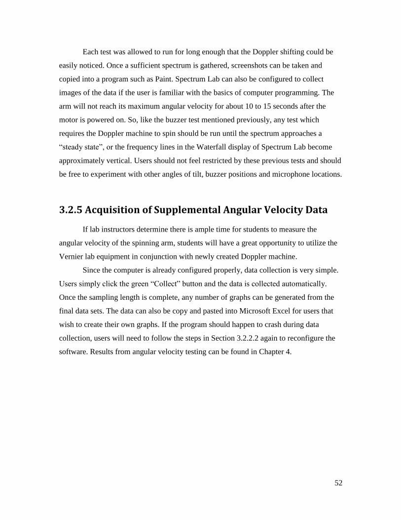
52
Each test was allowed to run for long enough that the Doppler shifting could be
easily noticed. Once a sufficient spectrum is gathered, screenshots can be taken and
copied into a program such as Paint. Spectrum Lab can also be configured to collect
images of the data if the user is familiar with the basics of computer programming. The
arm will not reach its maximum angular velocity for about 10 to 15 seconds after the
motor is powered on. So, like the buzzer test mentioned previously, any test which
requires the Doppler machine to spin should be run until the spectrum approaches a
“steady state”, or the frequency lines in the Waterfall display of Spectrum Lab become
approximately vertical. Users should not feel restricted by these previous tests and should
be free to experiment with other angles of tilt, buzzer positions and microphone locations.
3.2.5 Acquisition of Supplemental Angular Velocity Data
If lab instructors determine there is ample time for students to measure the
angular velocity of the spinning arm, students will have a great opportunity to utilize the
Vernier lab equipment in conjunction with newly created Doppler machine.
Since the computer is already configured properly, data collection is very simple.
Users simply click the green “Collect” button and the data is collected automatically.
Once the sampling length is complete, any number of graphs can be generated from the
final data sets. The data can also be copy and pasted into Microsoft Excel for users that
wish to create their own graphs. If the program should happen to crash during data
collection, users will need to follow the steps in Section 3.2.2.2 again to reconfigure the
software. Results from angular velocity testing can be found in Chapter 4.

53
4. Results
Developing reliable results for this experiment proved to be difficult due to the
number of variables that affect the signal that is observed by users in Spectrum Lab.
Minor variations in computer and laboratory configurations can have dramatic
consequences on data collection, and therefore, completely skew results.
When testing during C Term 2009, it took the team a full seven weeks to develop
a comprehensive set of tests that could be used to analyze all variables in the Doppler
equation individually. In Section 3.2.4, a list of tests was shown and these tests combined
the different buzzer positions and angular velocities with different angles of tilt. By
testing in this manner, and using three microphones simultaneously, a full data set was
collected.
During the preliminary stages of these tests, several problems were encountered
that brought data collection to a standstill while the issues were resolved. In an attempt to
gather data more conveniently, two laptops were brought to the lab and setup with the
proper software. However, as the team would soon learn, Spectrum Lab is not currently
compatible with Windows Vista. When testing was performed in the anechoic chamber in
the attic of Olin Hall, the laptops recorded very weak signals that would only be heard
when the buzzer was passing directly in front of the microphone. The conclusion reached
from this test was that the anechoic chamber was absorbing all sound that was not
directed straight into the microphone. This was a costly assumption as this implied that
the laboratory walls and floors were reflecting a majority of the sound waves and echoing
back into the room, causing extra harmonic frequencies to be picked up by Spectrum Lab.
In reality, the only thing that was wrong was that the laptop had Microsoft Vista and the
signal is not processed correctly, resulting in inconclusive results.
Another problem that arose was during testing of the buzzers. A test of the
directionality of the sound from the buzzer was performed by holding a microphone at
different distances from the top, bottom, and side of the buzzer housing. To add to this
problem, a laptop with Microsoft Vista was being used to record results. This test
indicated that the buzzer was four times as loud from the top as the bottom, and three
times as loud from the top as the side. This test also lent credibility to the theory that the

54
anechoic Chamber was absorbing stray sound and the microphone was only picking up
short bursts of sound.
Once these issues were resolved, all tests were performed again using Microsoft
XP as the operating system. These tests provided the most reliable results which are
detailed in the next sections.
4.1 Doppler Testing Results
The tests used for gathering Doppler data were described in Section 3.2.4.
Performing the tests in this systematic manner allows for isolation of each variable of the
Doppler equations. As a result of these 10 tests, and using three microphones for each
test, 30 screenshots were collected from Spectrum Lab. These screenshots represent
different buzzer positions, different angles of tilt, and various receiver distances from the
source. While more data could be collected for other angles and other buzzer positions,
the results for any angles between 0 and 45 degrees will most likely turn out to resemble
a mix of the results from the testing at 0 degrees and the testing at 45 degrees. Assuming
that assumption is correct, the results for angles from 45 to 90 degrees would be some
combination of the results from testing at 45 degrees and testing at 90 degrees. Following
this same logic, adjusting the buzzer position would have similar consequences on the
resulting spectra. Hence, these 30 data sets provided a generous sample size and
sufficient information to draw some conclusions from. The full results of these tests can
be found in Appendix A.
One of the goals of this project was to improve the signal quality by reducing
noise and vibrations in the system. Figure 37 on the next page shows the data that was
collected by the previous group.
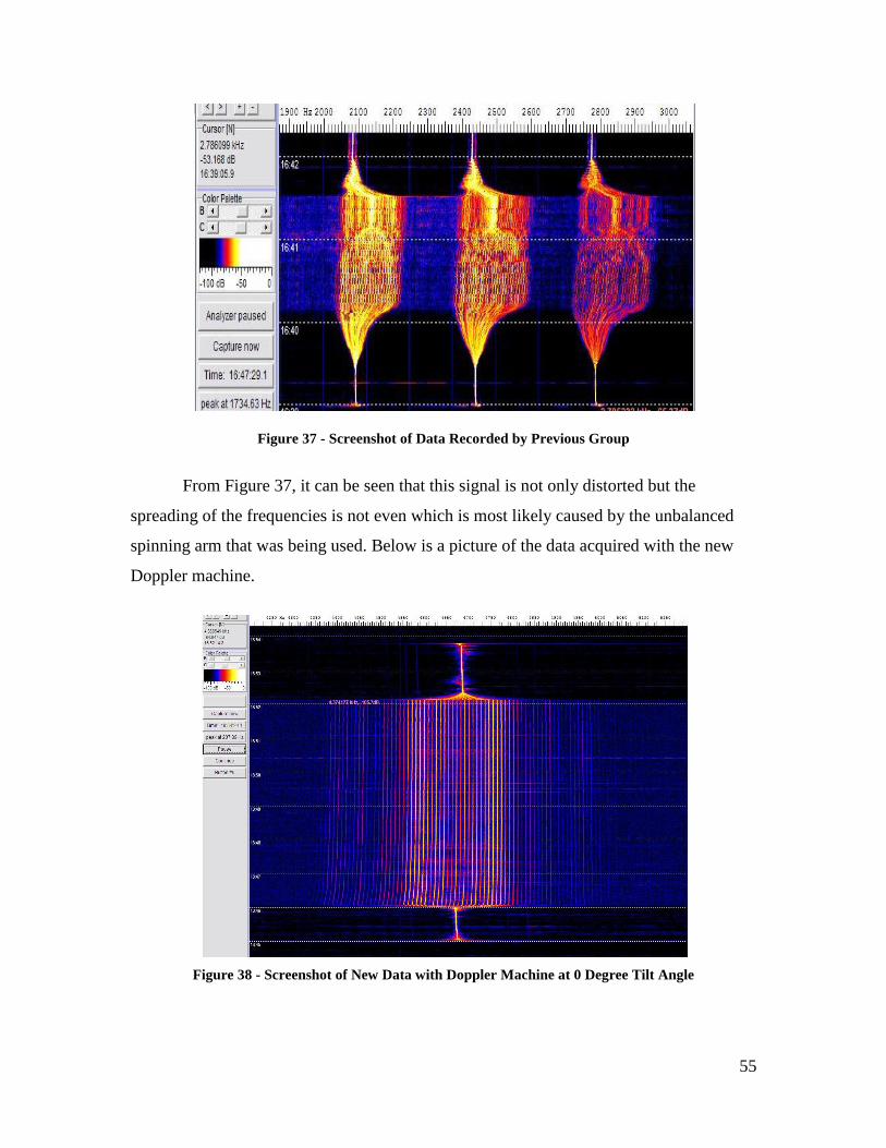
55
Figure 37 - Screenshot of Data Recorded by Previous Group
From Figure 37, it can be seen that this signal is not only distorted but the
spreading of the frequencies is not even which is most likely caused by the unbalanced
spinning arm that was being used. Below is a picture of the data acquired with the new
Doppler machine.
Figure 38 - Screenshot of New Data with Doppler Machine at 0 Degree Tilt Angle

56
The image in Figure 38 is simply much better looking and easier to interpret. The
spreading of frequencies happens very smoothly and the shifting is approximately even in
both directions. This indicates that, if nothing else, the new design was well balanced and
less prone to vibration, which in turn eliminated noise from the vibration of the machine.
The tapered edges on the new spinning arm also help the blade move through the air with
less resistance which reduces noise even further. Another sample is provided below that
shows one test which requires the machine to be tilted.
Figure 39 - Screenshot of New Data with Doppler Machine at 90 Degree Tilt Angle
Again, the smooth spreading of the frequencies is observed as well as a smooth
convergence when the machine is decelerating. However, this is an interesting result.
Consider a case where the receiver is directly in the center of the spinning arm rather than
outside the circular path. From this position, the relative velocity between the source and
the receiver are constant since the buzzer is at a fixed distance from the receiver. This
implies that there should be no Doppler shifting with the microphone in this position.
Figure 31 shows test results from a microphone that was in the center of the spinning
arm, but placed at the other end of the lab and separated by about 25 feet. The interesting
thing about this image is that it does show Doppler shifting, but, the harmonic
frequencies are most intense in the range of the rest frequency of the buzzer. This is a

57
great result and implies that the machine is functioning properly and the computers are
working.
In an attempt to confirm this result, we took a microphone and held it as close as
possible to the center of the spinning arm. This test did show some Doppler shifting, but
the intense center frequencies were more intense and more tightly grouped around the
resonant frequency of the buzzer. This phenomenon is assumedly caused by the reflection
of sound waves off the walls. It is believed that running this test in the anechoic chamber
would reduce the reflection and produce a result that showed approximately no Doppler
shifting. This test once again confirmed that, at the very least, the machine well balanced
and functioning properly, rotating at a constant speed. At best, these results are extremely
accurate if you discount the signal variations caused by reflection in the room.
4.2 Angular Velocity Testing Results
Performing these tests takes very little time once preparations are made and the
experiment is completely set up. The manner in which the Vernier equipment is fastened
to the motor mount allows for some error in the measurements. Also, using a rubber band
as the belt for the gears could cause additional error as the rubber band might slip slightly
during rotation. However, from observing this testing in progress, there did not appear to
be any significant problems due to these factors and a tolerance of five percent was
recorded. The graph in Figure 40 on the next page shows the results of the testing of
angular velocity versus buzzer distance from the center of the arm. A trend line was
included to emphasize the accuracy of these measurements.

58
Figure 40 – Results from Test of Angular Velocity (rev/min) vs. Buzzer Distance from Center of Arm
(cm) with Linear Trendline Shown
From this graph, the relationship between angular velocity and buzzer distance
from the center of the arm is seen to be approximately linear. This gives further weight to
the notion that the Vernier equipment is indeed properly attached, despite its humble
appearance, and that the rubber band provides adequate friction to be used as a belt for
the gears. Data was recorded in increments of two centimeters until the entire arm length
had been completed. The graphs from these individual tests are hard to analyze due to the
high sample rate that was used. Despite this fact, the data was stored and calculations
were made of the average angular velocity for each point. This raw data had to be scaled
by a factor of 1.44 to account for the gear ratios. An Excel spreadsheet containing all data
acquired during this testing has been included with the final submission of this report as a
supplementary document.
300
350
400
450
500
550
600
650
1217222732
An
gula
r V
elo
city
[re
v/m
in]
Buzzer Distance from Center of Arm [cm]
Angular Velocity vs Buzzer Radius
Angular Velocity ± 5%

59
5. Conclusions
These results are a vast improvement over the limited data that was provided from
the previous group, and this machine was capable of generating repeatable data. In
addition, the Vernier equipment was utilized which combined existing lab equipment
with the new Doppler machine and allowed for a completely new set of data to be
collected.
In the future, full spectral analysis needs to be done to determine the exact
characteristics and properties of the harmonic frequencies. Once that is completed, a
general formula needs to be derived to calculate the expected frequency of all harmonics.
Investigating the harmonic properties of this system should allow a project team to
synthesize the results and help create a laboratory experiment.
Also, testing needs to be carried out in an isolated environment. The results of
isolation testing should reduce the current results to the expected result in which there is
no Doppler shifting when tilted at 90 degrees. If that result can be achieved in either the
anechoic chamber or outside that would imply that this device is ideally designed and
functioning exactly as it was intended to function.
Once all this information is gathered, a student participating in this experiment
should be able to calculate the speed of rotation of the arm, the distance of the source
from the receiver, or given the rest frequency of the buzzer, the expected frequency shift
can be calculated. Characterizing the properties of all the harmonic vibrations in this
system is certainly beyond the scope of freshman level physics courses at WPI. However,
this device can still be used to show the basic properties of the Doppler effect, as well as
introducing the basic concept of harmonic vibrations. Along with the Spectrum Lab
software, students can observe the data collection process in real-time and watch the
spectra change as the experiment configurations are altered. This interactive hands-on
approach may appeal to certain students and encourage them to pursue their interests in
physics.
For a freshman level lab course, this should provide more than enough activity to
fill up the lab session if time is managed properly. Also, this allows instructors to pose a
number of different problems to students in which they solve for a certain variable given

60
the value of another variable. One of the main goals was to create a fun new lab that
would get everyone actively involved in the experiment, and show an old concept in a
new light. Research indicates that once the data has been more thoroughly analyzed and
characterized, this experiment could definitely become a fun and effective new way to
teach students about the Doppler effect.

61
6. Recommendations
Throughout the semester, substantial progress was made on this project. The
Doppler machine was completely redesigned with minimal noise and vibration, and tests
were performed that resulted in higher quality, repeatable results. Since these results
represent only a portion of total data collection in an ongoing project, there are several
ways in which this experiment could be improved when considering future work.
When selecting component parts to use on the Doppler machine, various
manufacturers were contacted for advice about how to choose the best parts for this
particular experiment. During one phone conversation with a sales representative from
Floyd Bell Inc. Sound Solutions, the suggestion was made that this experiment should be
done with a lower frequency buzzer to achieve more dramatic and noticeable Doppler
shifting. This theory was not corroborated by any testing as there was not sufficient time
to order the new parts. However, in the future, this is certainly something to consider, and
Floyd Bell Inc. has a variety of different buzzers that are slightly more expensive, but
much higher quality than the current buzzers. For more information visit their website at
http://www.floydbell.com/.
The one feature of the old Doppler device that was not included in the new design
was the use of the Variac to control the speed of the motor. Sliding the buzzers up and
down the length of the arm will change the weight distribution and cause the arm to spin
faster when the buzzers are closer to the center. However, with a Variac in the system,
the user has more precise control over the motor speed. Therefore, it is recommended that
a new Variac be purchased and included in the new Doppler machine.
The next recommendation is that alternate environments should be used to collect
some data. The labs in Olin Hall have very solid walls and it is believed that a large
percentage of the sound signal is being reflected back into the room, thus increasing the
number of harmonic frequencies observed in the spectrum. To determine the actual
impact of the reflection of the sound spectrum, a computer should be installed in the attic
in Olin Hall and more testing should be done in the anechoic chamber. This chamber
should theoretically absorb all sound waves that are not incident on the receiver, thus
allowing for the acquisition of a raw sound signal with no interference from reflected

62
waves. From these results, an observer should be able to compare the difference in
signals from the two environments. The anechoic chamber is rather small though, which
does not allow for any long range testing. For this purpose, a room with a much greater
volume such as a large hall would most likely help eliminate echoing. Attempting this
test outside could certainly be useful and would definitely reduce echoing, but this can
only be done if a laptop can be installed with the proper software and configured
correctly.
Finally, the last thing that could be done to improve this experiment is to purchase
some high quality microphones. The microphones that were provided by the school and
used for testing performed surprisingly well for the price, but spending some extra money
for microphones that are more sensitive may be the final way to improve signal quality. It
is not known what affect a new microphone would have on the results, but it is
recommended that the feasibility and cost effectiveness of this issue be investigated.
The recommendations given here should be used as a guideline of possible ways
in which to improve upon this project. That is not to say that there are no other
improvements that could be made, as there may be other ways to improve the Doppler
machine and the experimental setup. However, from the research conducted over the
previous semester, it is believed that these are the best actions to take in moving forward
with this research and making this experiment usable as an undergraduate lab.

63
Bibliography
Filkin, D. (1997). Stephen Hawking's Universe: The Cosmos Explained. Basic Books.
Girgis, A. M. (2009, April 13). Doppler Effect Mathematics and the Inkscape Vector
Graphics Software. (C. Teske, Interviewer) Worcester, MA.
Pydynkowski, K., Lessard, B., Perry, K., McGinley, J., & Jones, B. (2009). Ongoing
Advancement of the Physics Toolbox. Interdisciplinary Qualifying Project, Worcester.
Saba, M. M., & Antonio da S. Rosa, R. (2003). The Doppler Effect of a Sound Source
Moving in a Circle. The Physics Teacher , 41.
Serway, R. A., & Beichner, R. J. (2000). Physics For Scientists and Engineers (5th
Edition ed.). Orlando, Florida, United States Of America: Saunders College Publishing.

64
Appendix A – Complete Results of Doppler Test
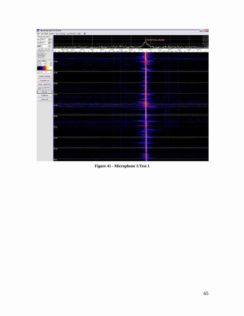
65
Figure 41 - Microphone 1/Test 1

66
Figure 42 - Microphone 2/Test 1

67
Figure 43 - Microphone 3/Test 1
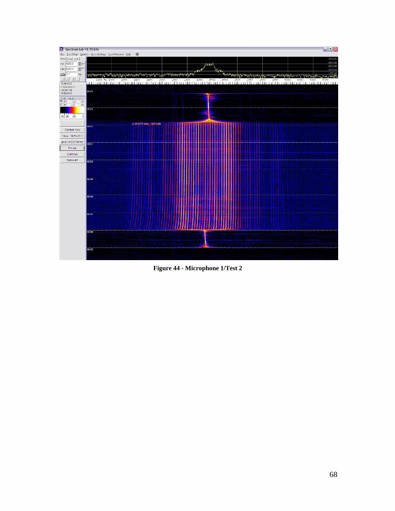
68
Figure 44 - Microphone 1/Test 2
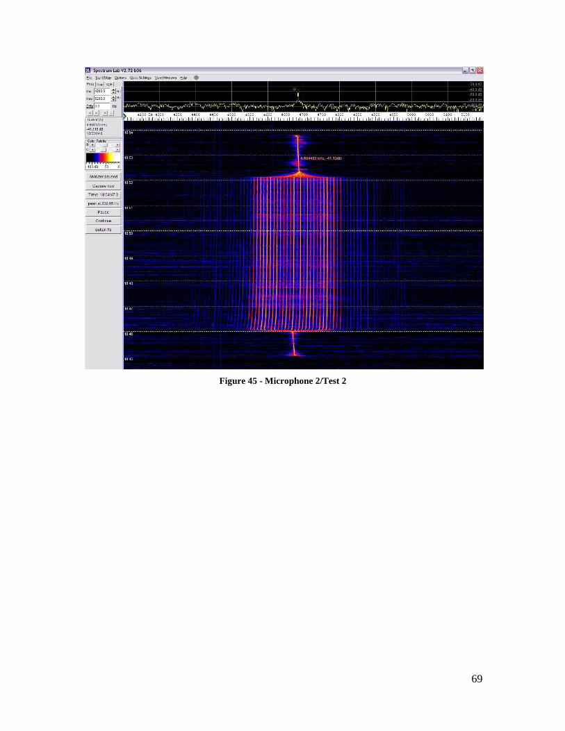
69
Figure 45 - Microphone 2/Test 2

70
Figure 46 - Microphone 3/Test 2

71
Figure 47 - Microphone 1/Test 3

72
Figure 48 - Microphone 2/Test 3

73
Figure 49 - Microphone 3/Test 3

74
Figure 50 - Microphone 1/Test 4

75
Figure 51 - Microphone 2/Test 4
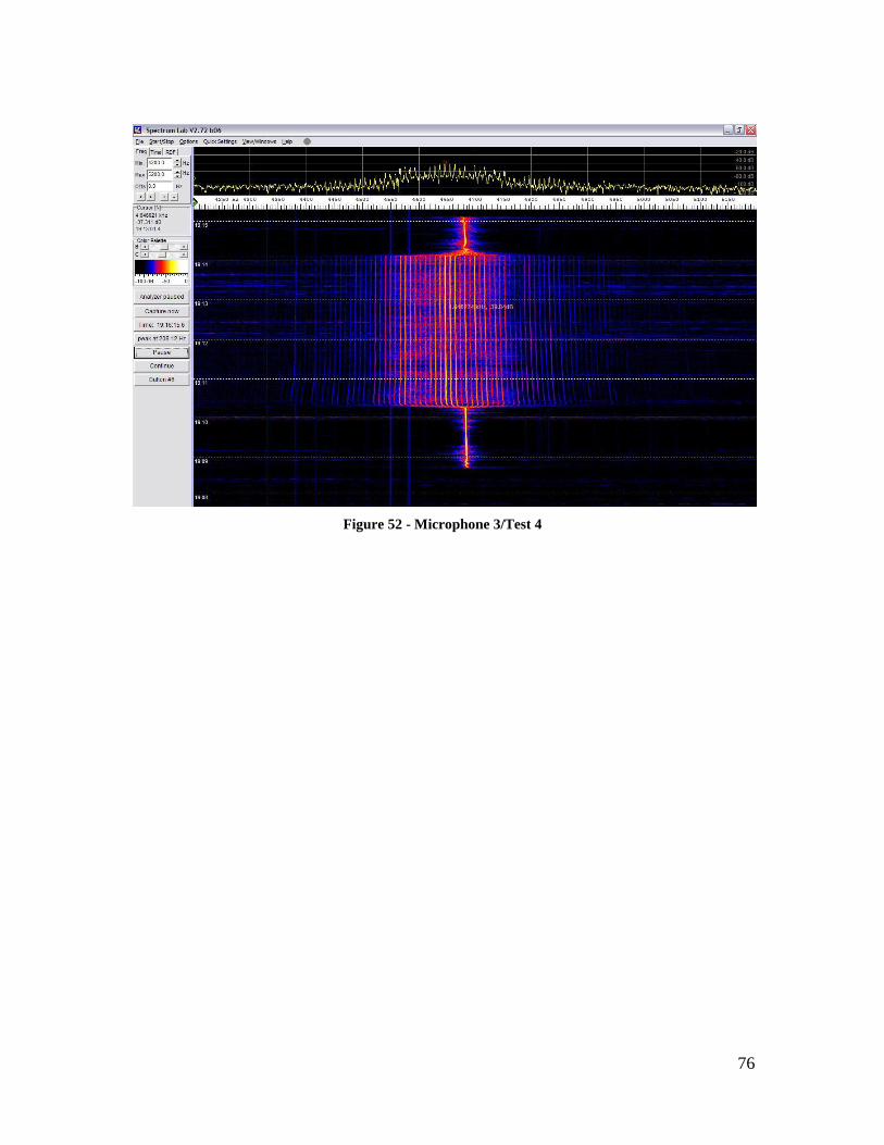
76
Figure 52 - Microphone 3/Test 4

77
Figure 53 - Microphone 1/Test 5

78
Figure 54 - Microphone 2/Test 5
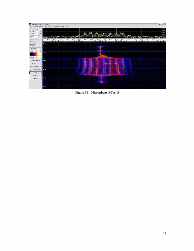
79
Figure 55 - Microphone 3/Test 5

80
Figure 56 - Microphone 1/Test 6

81
Figure 57 - Microphone 2/Test 6

82
Figure 58 - Microphone 3/Test 6

83
Figure 59 - Microphone 1/Test 7

84
Figure 60 - Microphone 2/Test 7

85
Figure 61 - Microphone 3/Test 7

86
Figure 62 - Microphone 1/Test 8

87
Figure 63 - Microphone 2/Test 8

88
Figure 64 - Microphone 3/Test 8

89
Figure 65 - Microphone 1/Test 9

90
Figure 66 - Microphone 2/Test 9

91
Figure 67 - Microphone 3/Test 9

92
Figure 68 - Microphone 1/Test 10

93
Figure 69 - Microphone 2/Test 10

94
Figure 70 - Microphone 3/Test 10