an experimental investigation of hot water and …infohouse.p2ric.org/ref/43/42473.pdfunc-hrr...
TRANSCRIPT

REPORT 1\10. 290
by Paul T. Imhoff, Cass T. Miller, Angela Frizzell, Laura A. Vancho, Simon N. Gleyzer, l taru Qkuda, and John F. ‘McBride
Department o f Environmental Sciences and Engineering University of North Carolina a t Chapel Hill
January 1995


UNC-HRR 1-95-290
AN EXPERIMENTAL INVESTIGATION OF HOT WATER AND COSOLVENT FLUSHING FOR REMEDIATION OF NAPL-CONTAMINATED AQUIFERS
Paul T. Imhoff Research Assistant Professer
Cass T. Miller Associate Professor
Angela Frizzell and Laura A. Vancho Research Assistants
Simon N. Gleyzer and Itaru Okuda Post-Doctoral Research Associates
John F. McBride Research Assistant
Department of Environment a1 Sciences and Engineering The University of North Carolina Chapel Hill, North Carolina 27599
The research on which this report is based was financed in part by the United States Department of the Interior, Geological Survey, through The North Carolina Water Re- sources Research Institute.
Contents of the publication do not necessarily reflect the views and policies of the United States Department of Interior, nor does mention of trade names or commercial products constitute their endorsement by the United States Government.
WRRI P r o j e c t No, 70117 Agreement No. 14-08-0001-G2037
USGS P r o j e c t No. 12 (FY ' 9 2 ) January 1995

One hundred fifty copies of this report were printed at a cost of $1,351.50 or $9.01 per copy.

Acknowledgements
This work was performed within the Department of Environmental Sciences and Engi-
neering of the School of Public Health at the University of North Carolina at Chapel
Hill. We thank Mr. Randall Goodman and Mr. Cliff Burgess for their assistance in de-
signing and fabricating the laboratory experimental devices.
.. 11


Abstract
Pump-and-treat is the most commonly used method for removing contaminants
from groundwater but has proven ineffective in the case of nonaqueous phase liquids
(NAPLs). Two methods that have been used to enhance recovery of crude oil, hot wa-
ter and alcohol flooding, were investigated in the laboratory as a means of enhancing
the dissolution and recovery of NAPLs in groundwater. A ubiquitous NAPL, tetra-
chloroethylene (PCE), was chosen for recovery in this investigation.
In investigating hot water flooding, the temperature-dependence of several fluid prop-
erties was first evaluated over the range from 5°C to 40°C. Among fluid properties, the
most substantial variations with temperature were seen in PCE diffusivity and aque-
ous and PCE phase viscosity: PCE diffusivity increased by 162%) while the aqueous
and PCE phase viscosities increased by 51% and 31% respectively. PCE solubility was
shown experimentally to have a minimum value near 20°C (225 mg/l), which is sub-
stantially higher than the majority of published values. Steady-state dissolution experi-
ments were then conducted in a jacketed, 2.5-cm internal diameter by 1-cm long column,
with both glass beads and a natural coastal sand as packing material. Mass transfer rate
coefficients increased with temperature and with NAPL saturation; the mass transfer
rate coefficient increased by a factor of two as temperatures rose from 5°C to 40°C. A
comparison of the results with existing dimensionless correlations for mass transfer in
porous media elucidated the role of diffusivity and the Schmidt Number (Sc) in such
models. Overall, the data suggest that addition of heated water to a pump-and-treat
system could yield greater recoveries of dissolved PCE than with conventional methods,
... 111


although the improvement is not dramatic over the temperature range studied. How-
ever, heated water is expected to be much more beneficial for NAPLs with lower boiling
points.
A second promising approach for enhanced remediation of NAPL-cont aminated aquifers
is the use of chemical cosolvents to enhance the effciency of conventional pump-and-
treat remediation, Miscible cosolvents such as alcohol promote dissolution of NAPLs
into the aqueous phase; reduce interfacial tension between NAPLs and water, thus en-
hancing NAPL mobilization; and may alter physical properties that control or influence
subsurface contaminant transport and fate processes. Methanol is an attractive cosol-
vent because it is readily available) inexpensive, and mutually miscible with water and
many NAPLs. For these reasons it was selected for study for the remediation of PCE-
contaminated porous media.
The PCE/methanol/water system was studied to evaluate the effect of methanol con-
centration on interfacial tension, equilibrium phase composition, and phase density.
When volumetric methanol concentrations in the aqueous phase increased from 0% to
SO%, interfacial tension between the NAPL and aqueous phases decreased by 73%, aque-
ous phase PCE solubility increased from 225 mg/l to 9140 mg/l in an approximately
log-linear fashion) and the equilibrium NAPL phase densities changed by less than 1%.
Methanol predominately partitions into the aqueous phase and does not promote NAPL
swelling and uncontrolled mobilization of free-phase NAPL. A subsequent experiment
evaluated the effectiveness of a 60% methanol/40%water mixture on the removal of
residual PCE from a glass bead medium. Because of the reduction in interfacial tension,
this mixture resulted in the mobilization of 12% of the PCE from the column. Subse-
quent removal of PCE with the methanol/water mixture was by dissolution, and mea-
sured mass transfer rate coefficients for a portion of the medium were within a factor of
1v


five of predictions from existing correlations. The data suggest that flooding with meth-
anol/water mixtures significantly decreases the number of pore volumes required to re-
move NAPLs from contaminated aquifers.
V


Table of Contents
Page
.. Acknowledgements . . . . . . . . . . . . . . . . . . . . . . . 11
... Abstract . . . . . . . . . . . . . . . . . . . . . . . . . . . . . 111
List of Figures . . . . . . . . . . . . . . . . . . . . . . . . . . xii
List of Tables . . . . . . . . . . . . . . . . . . . . . . . . . . . xv
Summary and Conclusions . . . . . . . . . . . . . . . . . . . xvii
Recommendations . . . . . . . . . . . . . . . . . . . . . . . xx
1 Thermally EnhancedNAPLDissolution . . . . . . . 1
1.1 Background . . . . . . . . . . . . . . . . . . . . . . 1
1.1.1 Introduction . . . . . . . . . . . . . . . . . . . . . . . 1
1.1.2 Thermal Techniques for Enhanced Oil Recovery . . . . . . . . 2
1.1.3 Thermal Techniques for Remediation of Contaminated
A q u i f e r s . . . . . . . . . . . . . . . . . . . . . . . . . 3
vi


1.1.4 Summary of Thermal Techniques . . . . . . . . . . . . . . 6
1.2 ExperimentalMethods . . . . . . . . . . . . . . . . . 7’
1.2.1 Materials . . . . . . . . . . . . . . . . . . . . . . . . 7’
1.2.2 Temperature Control . . . . . . . . . . . . . . . . . . . 8
1.2.3 Interfacial Tension . . . . . . . . . . . . . . . . . . . . 9
1.2.4 Dissolution . . . . . . . . . . . . . . . . . . . . . . . . 10
1.2.4.1 C o l u m n Des ign . . . . . . . . . . . . . . . . . . 10
1.2.4.2 Sampling . . . . . . . . . . . . . . . . . . . . . 13
1.2.4.3 UV Spectrophotometry . . . . . . . . . . . . . . . 15
1.3 Results . . . . . . . . . . . . . . . . . . . . . . . . 16
1.3.1 Solubility . . . . . . . . . . . . . . . . . . . . . . . . 16
1.3.2 PhaseDensity . . . . . . . . . . . . . . . . . . . . . . 17’
1.3.3 Interfacial Tension . . . . . . . . . . . . . . . . . . . 18
1.3.4 Viscosity . . . . . . . . . . . . . . . . . . . . . . . . . 21
1.3.5 Molecular Diffusion Coefficient . . . . . . . . . . . . . . . 22
vii


1.3.6 Dissolution . . . . . . . . . . . . . . . . . . . . . . . . 22
2.9.6.1 Mass Transfer Rate Coeficient . . . . . . . . . . . . 22
j.S.6.2 Modeling . . . . . . . . . . . . . . . . . . . . . . 27
1.4 Discussion . . . . . . . . . . . . . . . . . . . . . . . 40
1.4.1 Physical and Chemical Properties . . . . . . . . . . . . . . 40
1.4.2 Mobilization . . . . . . . . . . . . . . . . . . . . . . . 41
1.4.3 Dissolution . . . . . . . . . . . . . . . . . . . . . . . . 42
2 Alcohol Flushing . . . . . . . . . . . . . . . . . 44
2.1 Background . . . . . . . . . . . . . . . . . . . . . . 44
2.1.1 Introduction . . . . . . . . . . . . . . . . . . . . . . . 44
2.1.2 Alcohol Flooding for Enhanced Oil Recovery . . . . . . . . . 44
2.1.3 Remediation of Contaminated Aquifers by Alcohol Flooding . . 47
2.1.4Summary . . . . . . . . . . . . . . . . . . . . . . . . 49
2.2 Experimental Methods . . . . . . . . . . . . . . . . . 50
2.2.1 Overview . . . . . . . . . . . . . . . . . . . . . . . . 50
... Vlll


2.2.2 Materials . . . . . . . . . . . . . . . . . . . . . . . . 51
2.2.3 Equilibrium Phase Partitioning: Generator Columns . . . . . 52
2.2.4 Equilibrium Phase Partitioning: Batch Experiments . . . . . . 57
2.2.4.1 Sample Collection and Dilution . . . . . . . . . . . 58
2.2.4.2 Gas Chromatograp hie Analysis . . . . . . . . . . . . 59
2.2.4.3 Calibration Standards . . . . . . . . . . . . . . . 60
2.2.4.4 Karl Fischer Coulometric Titrations . . . . . . . . . 61
2.2.5 Equilibrium Phase Partitioning: Titrations . . . . . . . . . .
2.2.6 Phase Density . . . . . . . . . . . . . . . . . . . . . . 62
61
2.2.7 Interfacial Tension . . . . . . . . . . . . . . . . . . . . 63
2.2.8 Mobilization and Dissolution . . . . . . . . . . . . . . . . 63
2.3.1 Phase Partitioning . . . . . . . . . . . . . . . . . . . . 67
2.3.1.1 PCE Solubility in Methanol/Water Mixtures: Data . . . 67
2.3.1.2 PCE Solubility in Methanol/Water Mixtures: Model . . . 73
ix


2.3.1.3 Methanol Solubility in Nonaqueous Phase . . . . . . . 74
2.3.1.4 Water Content in Nonaqueous Phase . . . . . . . . . 75
2.8.1.5 Ternary Phase Diagram: Data . . . . . . . . . . . . 76
2.3.1.6 Ternary Phase Diagram: Model Predictions . . . . . . 79
2.3.2 Phases Density . . . . . . . . . . . . . . . . . . . . . . 82
2.3.3 Interfacial Tension . . . . . . . . . . . . . . . . . . . . 86
2.3.4 Viscosity . . . . . . . . . . . . . . . . . . . . . . . . . 88
2.3.5 Molecular Diffusion Coefficient . . . . . . . . . . . . . . . 88
2.3.6 Mobilization . . . . . . . . . . . . . . . . . . . . . . . 93
2.3.7 Dissolution . . . . . . . . . . . . . . . . . . . . . . . . 96
2.3.8 Mass Transfer Rate Coefficient . . . . . . . . . . . . . . . 99
2.4 Discussion e e e e e * e . . 107
2.4.1 Physical and Chemical Properties . . . . . . . . . . . . . .
2.4.2 Mobilization . . . . . . . . . . . . . . . . . . . . . . . 108
2.4.3 Dissolution . . . . . . . . . . . . . . . . . . . . . . . . 110
107
X


References . . . . . . . . . . . . . . . . . . 113
xi


List of Figures
1 Construction of mass transfer column . . . . . . . . . . . . . . . . . . . 11
2 Emplacement of NAPL residual . . . . . . . . . . . . . . . . . . . . . 12
3 Sampling from column . . . . . . . . . . . . . . . . . . . . . . . . . . . 14
4 Variation of PCE water solubility with temperature . . . . . . . . . . . . . 17
5 PCE and aqueous phase density . . . . . . . . . . . . . . . . . . . . . 19
6 Effect of temperature on PCE/water interfacial tension . . . . . . . . . . . 20
7 Viscosity of PCE and aqueous phases . . . . . . . . . . . . . . . . . . . 21
8 Molecular diffusion coefficient of PCE in water . . . . . . . . . . . . . . . 23
9 Mass transfer rate coefficient versus temperature for glass bead
experiments . . . . . . . . . . . . . . . . . . . . . . . . . . . . . . 27
10 Mass transfer rate coeEcient versus R e for glass bead experiments . . . . . . 28
11 Mass transfer rate coefficient versus temperature for Camp Lejeune
experiments . . . . . . . . . . . . . . . . . . . . . . . . . . . . . . 29
12 Mass transfer rate coefficient versus Re for Camp Lejeune experiments . . . . 30
xii


13 Comparison of measured Sh with predicted Sh from existing correlations. . . 32
14 Comparison of measured S ~ / S C ' . ~ with predicted S ~ / S C ' * ~ from existing
correlations. . . . . . . . . . . . . . . . . . . . . . . . . . . . . . 36
15 Maximum potential mass flux of PCE for representative conditions using
equations (6) and (7). . . . . . . . . . . . . . . . . . , . . . . . . . 43
16 Experimental setup using generator columns . . . . . . . . . . . . . . . 56
17 Schematic of experimental apparatus investigating enhanced remediation
with alcohol flushing. . . . . ,. . . . . . . . . . . . . . . . . . . . . 65
18 Data from a generator column experiment showing concentration
measurements from two columns in series over time. . . . . . . . . . . . . 68
19 PCE solubility in methanol/water mixtures. Error bars as so small as not
to be visible. . . . . . . . . . . . . . . . . . . . . . . . . . . . . . 74
20 PCE/methanol/water ternary diagram. Axes units are % mole fraction. . . . 78
21 PCE/methanol/water ternary diagram. Solid tie lines are experimental;
dashed tie lines are predicted from UNIQUAC. Units are % mole fraction. . . 83
22 Pure and batch-equilibrated NAPL densities. . . . . . . . . . . . . . . . 85
23 Aqueous phase densities at 22°C. . . . . . . . . . . . . . . . . . . . . 87
... Xlll


24 Interfacial tension between aqueous and nonaqueous phases as a function of
methanol volume fraction. Error bars are so small as not to be visible. . , . . 89
25 Viscosity of methanol/water mixturesfrom FZick [1991]. . . . . . . . . . . 91
26 Predicted diffusion coefficients of PCE in methanol/water mixtures. . . , . . 94
27 Distribution of PCE volumetric fraction and porosity in column. PCE
volumetric fraction is shown before and after displacement by water. . . . . 95
28 Distribution of PCE volumetric fraction and porosity in column. PCE
volumetric fraction is shown before and after methanol/water flush. . . . . . 97
29 Effluent PCE concentration versus pore volumes. . . . . . . . . . . . . . 98
30 PCE saturation versus time for x = 7.25 cm. . . . . . . . . . . . . . . . 101
31 Mass transfer rate coefficient versus changing PCE volumetric fraction for
sampling locations x = 1.75, 2.25, 2.75, and 3.25 cm. . . . . . . . . . . . 103
32 Comparison of predicted Sh from several correlations for NAPL dissolution
with the best-fit model from the 60% methanol/water dissolution
experiment. . . . . . . . . . . . . . . . . . . . . . . . . . . . . . 105
33 Predicted KI for PCE for representative conditions using equations (23) and
(24). . . . . . . . . . . . . . . . . . . . . . . . . . . . . . . . . 111
34 Maximum potential mass flux of PCE for representative conditions using
equations (23) and (24). . . . . . . . . . . . . . . . . . . . . . . . . 112
xiv


List of Tables
1 Properties of chemicals used in experiments . . . . . . . . . . . . . . . . 8
2 Mediaproperties . . . . . . . . . . . . . . . . . . . . . . . . . . . . 8
3 Measured C(L) and computed KT with 95% confidence intervals . . . . . . . 26
4 Mass transfer correlations . . . . . . . . . . . . . . . . . . . . . . . . 31
5 Parameter values used in mass transfer correlations . . . . . . . . . . . . . 33
6 Results of nonlinear regression . . . . . . . . . . . . . . . . . . . . . . 38
7 Results of linear regression . . . . . . . . . . . . . . . . . . . . . . . 39
8 Effect of temperature variation between 50C and 40°C on properties . . . . . 40
9 Measured PCE solubility in methanol/water mixtures at 20°C . . . . . . . . 69
10 Literature values of PCE aqueous solubility . . . . . . . . . . . . . . . .
11 Methanol concentrations in batch-equilibrated nonaqueous phase samples . . .
12 Nonaqueous phase water content . . . . . . . . . . . . . . . . . . . . .
13 Pure and batch-equilibrated NAPL densities at 20°C . . . . . . . . . . . .
70
75
76
84
xv


14 Aqueous phase densities at 22°C . Error bars are so small as not be be
visible . . . . . . . . . . . . . . . . . . . . . . . . . . . . . . . . 86
15 Batch-equilibrated interfacial tensions . . . . . . . . . . . . . . . . . . . 88
16 Viscosity of methanol/water mixtures from Flick 119911 . . . . . . . . . . . 90
17 Predicted diffusion coefficients of PCE from Wilke and Chang [1955] . . . . . 93
18 Effects of methanol increase from 0% to 60% methanol fraction on
properties . . . . . . . . . . . . . . . . . . . . . . . . . . . . . . . 107
xvi


Summary and Conclusions
1. A laboratory study was performed to investigate the utility of hot water and alcohol
flooding on the enhanced remediation of NAPL-contaminated aquifers. A ubiqui-
tous NAPL, tetrachloroethyene (PCE), was chosen as a representative contaminant.
2. Among fluid properties, the most substantial variations with temperature were seen
in PCE diffusivity and aqueous and PCE phase viscosity: PCE diffusivity increased
by 162%, while the aqueous and PCE phase viscosities decreased by 51% and 31%
respectively, for temperatures between 5°C to 40°C. PCE solubility was shown ex-
perimentally to have a minimum value near 20°C (225 mg/l), which is substantially
higher than the majority of published values.
3. Mass transfer rate coefficients were measured for the PCE/water system as a func-
tion of temperature, and increased by less than a factor of two as temperatures in-
creased from 5°C to 40°C. The mass transfer rate coefficient was found to vary with
approximately the square root of diffusivity, which is attained by the inclusion of
S C * * ~ in the mass transfer model. The best-fit value for the exponent of Sc was
.
0.48. The dependency of Sh on Sc has not been previously demonstrated for the
dissolution of NAPL ganglia, although it was postulated by previous investigators.
4. The addition of heated water increased the maximum potential mass flux for PCE
dissolution by a factor of two as the temperature increased from 5°C to 60°C. This
increase is not large, and in many situations may not be justified given the added
expense of heating water.
xvii


5. Methanol was investigated as a cosolvent for the removal of PCE from the sub-
surface. The PCE/methanol/water system was studied to evaluate the effect of
methanol concentration on interfacial tension, equilibrium phase composition, and
phase density. When volumetric methanol concentrations in the aqueous phase in-
creased from 0% to 60%) interfacial tension between the nonaqueous and aqueous
phases decreased by 73%) aqueous phase PCE solubility increased from 225 mg/l to
9140 mg/l in an approximately log-linear fashion, and the equilibrium nonaqueous
phase density changed by less than one percent.
6. The phase partitioning behavior of the PCE/methanol/water system was predicted
using UNIQUAC (Abrums and Pruusnitz, 1975). The predictions were in reason-
able agreement with experimental data, suggesting that such models may be used in
lieu of extensive experimentation to predict the phase partitioning behavior of other
NAPL/alcohol/water systems.
7. Methanol predominately partitions into the aqueous phase and does not promote
NAPL swelling. Thus, it is not expected to have as dramatic an effect on NAPL
mobilization as other alcohols which strongly partition into the nonaqueous phase.
In certain situations uncontrolled mobilization of free-phase NAPL is undesirable.
8. A 60% methanol/water mixture was used to remediate a glass bead porous medium
contaminated with PCE at residual saturation. The addition of methanol to the
system resulted in the mobilization of 12% of the residual PCE from the column.
The remaining PCE was dissolved from the column at a significantly faster rate
than with water alone: only 30 pore volumes were required for remediation, while
a water flood would have required approximately 1000.
xviii


9. The mobilization of residual PCE during the 60% methanol/water flood was due
to two factors: a reduction in the interfacial forces holding trapped PCE droplets
within the porous medium, and an increase in the density difference between PCE
and the aqueous phase. PCE at relatively high residual saturation located above
fine microlayers in the porous medium was readily mobilized.
10. A unique x-ray system was used to nondestructively measure the changing amount
of PCE in the porous medium during the alcohol flood. Using these measurements,
mass transfer rate coefficients were determined for PCE dissolution into a 60%
methanol/water mixture. Predictions for mass transfer rate coefficients from ex-
isting correlations were within a factor of five of data measured in the upper portion
of the column.
11. The addition of methanol increased the maximum potential mass flux for PCE dis-
solution by one order of magnitude as the methanol volumetric fraction increased
from 0% to 60%. This dramatic improvement in mass flux is due to the increase in
aqueous phase PCE solubility.
12. Alcohol flooding using methanol shows considerable promise for remediating NAPL-
contaminated aquifers.
xix


Recommendat ions
The need to obtain improved technologies for remediating NAPL-contaminated
aquifers has led to investigation of many enhanced remediation techniques. This study
has illustrated the limitations of hot water flooding over the temperature range from
5°C to 40°C and the benefits of flooding a PCE-contaminated porous medium with a
methanol/water mixture. Clearly, of the two techniques studied, alcohol flooding shows
more promise for the remediation of sites contaminated with PCE. However, for other
NAPLs with lower boiling points and for situations of rate-limited mass transfer, hot wa-
ter flooding may still be an effective technology.
The next steps are: (1) study the effect of heated water on the dissolution and mo-
bilization of NAPLs with lower boiling points; (2) better quantify the effect of methanol
or other alcohols on the mobilization of residual NAPLs; (3) study the interaction of al-
cohol and hot water flooding with heterogeneity, both of NAPL residual and soil struc-
ture, in two-dimensional laboratory experiments and with computer simulation; and (4)
compare the utility of alcohol and hot water flooding with surfactant or steam flooding.
This additional work, especially the investigation of heterogeneity using two-dimensional
laboratory experiments and computer simulation, will enable a better assessment of the
utility of these methods for field applications.
xx


1 Thermally Enhanced NAPL Dissolution
1.1 Background
1.1.1 Introduction
Conventional technologies for remediating contaminated aquifers are often ineffective
and excessively expensive. From a technological and economical point of view, it is clear
that there is a need for more efficient remediation methods. Therefore, development and
implementation of innovative treatment technologies for hazardous waste site remedia-
tion is an important problem.
Recently, different technologies have been suggested for enhancing the remediation of
contaminated aquifers, many of which have been used for years for enhanced recovery
of oil in petroleum engineering. To a certain extent, the knowledge, techniques and field
experiences gained in the oil industry are applicable to the problem of subsurface reme-
diation. In this report, results are summarized from an investigation of two techniques
for remediating sites contaminated with nonaqueous phase liquids (NAPLs) at residual
saturation below the water table: thermally enhanced remediation (or hot water flood-
ing), and alcohol flooding. Both techniques have been suggested for enhanced recovery
of oil in petroleum engineering. We begin by reviewing relevant investigations utilizing
thermal techniques in the petroleum literature and subsurface hydrology. Results are
then presented from a study of heated water on enhanced remediation. In the second
part of this report the investigation of alcohol flooding for enhanced remediation is dis-
cussed.
1

1.1.2 Thermal Techniaues for Enhanced Oil Recoverv
The removal of oil from subsurface strata using hot water and steam has been studied
within the petroleum industry for a number of years. Beginning with an early field test
reported by Stoval [1934], the use of steam and hot water for enhanced oil recovery has
progressed and become increasingly popular. Several recent reviews of investigations
and implementations of thermal methods in petroleum engineering have been reported
( B u e r g e r e t al., 1985; Boberg, 1988; Baibakov and Garushev, 1989).
Willman e t al. 119611 found that oil recovery by steam injection was always greater
than recovery by cold or hot water injection, and that using steam or hot water is of
greatest advantage with heavier oils, since there are significant viscosity reductions as
the temperature is increased. He demonstrated in laboratory experiments that steam in-
jection achieved greater oil recoveries than water floods and required less injected liquid
for these recoveries. Vobelc and Pryor 119721 conducted steam injection experiments on a
vertical column containing residual oil. The rates of oil recovery were between 66% and
84% immediately following steam breakthrough.
Edmondson [1965] conducted experiments with oils of viscosities 20 cp and 70 cp at
38°C. At 149"C, the oils had viscosities of 1.5 cp and 2.5 cp, respectively. He noted that
in flooding experiments at 149"C, piston-like displacement occurred with very little oil
produced after water breakthrough. Edmondson 119651 attributed the differences in wa-
terf'lood behavior of the two oils to differences in interfacial tension. In both the investi-
gation of Willman et al.
effect on the relative permeability ratio.
219611 and Edmondson [1965], temperature had a significant
2

Several researchers have tried to investigate the changes in the relative permeabilities of
oil and water with temperature (McCaflery, 1972; Lo and Mungan, 1973; Sufi e t al.,
1982; Quettier and Corre, 1988). However, results obtained from these investigations
have been contradictory.
1.1.3 Thermal Techniques for Remediation of Contaminated Aquifers
To a certain extent, the knowledge and techniques for thermal recovery of oil developed
in petroleum engineering are applicable to the problem of steam and hot water treat-
ment for subsurface remediation. There are, however, significant differences. Enhanced
oil recovery and aquifer remediation have two different goals: in enhanced oil recovery
the objective is to remove all large oil banks, while for aquifer remediation the objective
is to remove essentially all separate phase contaminant, even small amounts trapped at
residual saturation which result in aqueous phase concentrations below the maximum
contaminant level permitted. Because of these differing objectives, studies of enhanced
oil recovery neglect many processes which are import ant in contaminant remediation.
These include, for example, dissolution and transport of the organic contaminants in the
aqueous phase, and partitioning of the contaminant between the solid phase, aqueous
phase, and nonaqueous or oil phase (Hunt et al. 1988a and 1988b; Miller e t al., 1990;
Fukta et ak., 1992a and 1992b; Davis and Lien, 1993). These partitioning processes be-
tween phases may be rate limited.
The research efforts of Davis and Lien [1993] were focused on the use of moderately
hot water for enhancing the displacement of light oily wastes from sands. The oils filled
wat er-wet sand columns before displacement with heated water. Displacement experi-
ments were conducted over the range of 10°C to 50°C, with increases in oil recovery of
I
3

approximately 17% to 22% over this range. The main mechanism for the improvement
in oil recovery was the reduction of the oil viscosity.
A series of experiments conducted with trichloroethylene (TCE), a bicomponent mixture
of benzene and toluene, and a multicomponent gasoline demonstrated the feasibility of
steam injection for effective recovery of separate phase liquid contaminants ( H u n t e t aZ.,
1988b). While the NAPL could not be displaced from the column at water velocities up
to 15 m/day, steam was shown to displace the NAPL as a slug just ahead of the steam
condensation front, at injection velocities equivalent to 1.5 m/day. The temperature and
pressure data indicated multiphase flow behavior within the steam zone. Water flooding
following steam flooding demonstrated that contaminant removal was nearly complete.
The experimental results showed that only approximately one pore volume of steam was
required to achieve cleanup. Theoretical analysis of energy requirements showed that
steam displacement is economically attractive.
A series of one- and two-dimensional experiments were completed including the steam
displacement of TCE, a benzene-toluene mixture, and gasoline (S teward and UdeZZ, 1989;
Base l and UdebZ, 1989; Basel and Udell, 1991). Steward and Udell [1989] showed that
unlike isothermal processes where flow fingering and channeling phenomena limit the
mass transfer rates, the movement of the steam zone is controlled by temperature gra-
dients and mediurn heat capacities. Thus preferential channeling of steam is expected
to be of lesser importance. The stability of the condensation front was enhanced due
to heat losses from incipient fingers. Rather than small-scale fingering phenomena found
during the injection of a gas into a saturated porous media, only large-scale steam tongues
on the order of large scale heterogeneities are found during steam injection ( B a s e l and
Udell, 1989). For hydrocarbon compounds with lower vapor pressures than decane, the
distillation front would move with a velocity less than that of the steam condensation
4

front ( Y u a n and UdeZZ, 1993). This condition would be typical for the removal of a com-
pound such as diesel fuel, which is relatively nonvolatile. More volatile compounds such
as gasoline have been observed to form a liquid bank ahead of the steam condensation
front (Hunt e t aZ., 1988b).
The details of a numerical simulator developed for the purpose of modeling the steam re-
mediation process and validation of one-dimensional steam injection experiments (Hunt
e t al., 198813) were given by Fakta e t aZ. [1992a and 1992bl. A simple criterion was de-
rived for the optimal removal of NAPLs by steam displacement as a function of fluids
and porous medium characteristics. It was shown that the efficiency of the steam dis-
placement process depends on the NAPL vapor pressure at the steam temperature and
on the NAPL residual saturation. The results of this study indicate that NAPLs hav-
ing boiling points less than about 175°C may be efficiently removed as a separate phase
by steam injection. The displacement of NAPLs with boiling points above about 175°C
may not be as efficient as displacement of NAPLs with lower boiling points, although the
rate of removal is still much larger than with water and air injection methods.
Field studies were performed to verify the controllability of the movement of the steam
zone and to examine the effectiveness of steam injection to recover contarninants from
a spill site (UdeZZ, 1992). In this field experiment, steam was injected below the water-
table at a site in Livermore, California, contaminated with gasoline. After 24 days of
continuous steam injection, the data of cross-hole electrical three-dimensional tomogra-
phy indicated great success. Results from this study suggest that control over the move-
ment of the steam condensation front can be maintained if the large-scale permeability
field is known.
5 I

Western Research Institute developed the Contained Recovery of Oily Wastes (CROW)
process by adapting technology used for secondary petroleum recovery and for primary
production of heavy oil and tar sand bitumen (United States EPA, 1992). Steam and
hot-water displacement were used to move accumulated oily wastes and water to produc-
tion wells for aboveground treatment. Steam was injected below the deepest penetration
of organic liquids, while hot water was injected above the impermeable soil regions to
heat and mobilize the oil waste accumulations. This technology was tested both in the
laboratory and at pilot-scale at a wood-treatment site in Minnesota. Removal of NAPLs
in the pilot test were the same as that predicted by laboratory studies.
1.1.4 Summary of Thermal Techniques
The laboratory experiments and field scale results presented above indicate that ther-
mal methods can be technologically effective for removal of NAPLs from the subsurface.
These investigations have also shown that steam and hot water flooding involve several
complex processes. An important process which was not investigated in a systematic
manner is the effect of heated water on the rate of mass transfer from NAPLs at resid-
ual saturation. Hot water flushes of contaminated aquifer materials will not remove all
NAPLs by displacement; instead, trapped droplets will remain at residual saturation,
although the heated water will enhance the dissolution process. In addition, although
steam flooding will likely displace most NAPLs present, on the edges of the injection
zone water heated to temperatures much lower than the boiling point will exist and may
be in contact with NAPLs at residual saturation. In this region heated water will have
an important effect on NAPL dissolution. The focus of this investigation was to quantify
the effect of heated water on the rate of mass transfer for NAPLs at residual saturation,
4
6

as well as to determine any impact of heated water on mobilization of trapped NAPL
droplets .
,
1.2 Experimental Methods
1.2.1 Materials
The NAPL used in experiments was tetrachloroethylene (PCE), a denser-than-water
chlorinated solvent (HPLC grade, Sigma Chemical Co., Milwaukee, WI; and spectro
grade, Eastman Kodak Co., Rochester, NY). Methanol (HPLC grade, Mallinckrodt Spe-
cialty Chemicals Co., Paris, KY) was used as a solvent for aqueous PCE samples, and
methylene chloride (spectranalyzed grade, Fisher Scientific, Pittsburgh, PA) was used for
PCE extractions. Properties of these three chemicals are listed in Table 1. The water
used in all experiments was distilled and deionized to 50,000 ohm resistance (Mega-Pure
System, models D2 and MPllA, Corning Medical and Scientific, Corning, NY). For col-
umn experiments, the water was also deaerated by boiling, then stored under vacuum.
The two types of media used in experiments were glass beads and a natural coastal sand
referred to as the Camp Lejeune sand. The sand was gathered from well borings at the
Camp Lejeune Marine Corps Base in eastern North Carolina. The glass beads (size 50-
80 mesh, U.S. sieve, McMaster-Can Supply Company, Atlanta, GA) are slightly coarser
than the Camp Lejeune sand, but have a similar particle size distribution. Properties
of each medium are listed in Table 2. Both the beads and the sand are characterized by
very low total organic carbon (TOC) content, thereby minimizing sorption effects.
7

Table 1. Properties of chemicals used in experiments.
Property
Specific gravity' Dynamic viscositya (mPa s) Aqueous solubility' (mg/l) Boiling point ("C)
PCE Methanol Methylene Reference
1,623 0.791 1.327 L i d e 119901 0.93' 0.45 0.55b L i d e [1990] 220' miscibled 13,455e see notes 121 65 40 Lide [1990]
Chloride
Table 2. Media properties.
Particle density, p.
d50 is the median particle diameter. Uniformity coefficient = d60/d10
1.2.2 Temperature Control
Most of the experiments were conducted at multiple temperatures. Mass transfer and
solubility experiments were conducted with jacketed glassware and a water bath (series
8

9500, PolyScience Co., Niles, IL, adjustable to 0.l"C) that allowed for temperature con-
trol under a fume hood. Other experiments were performed at 10°C, 20°C and 40°C
in a constant temperature room (model ESI 4-5 WR, Environmental Specialties, Inc.,
Raleigh, NC), with an accuracy rating of f0.5"C.
1.2.3 Interfacial Tension
A ring-type tensiometer (model 70545, Central Scientific Company, Inc., Fairfax, VA)
was used to measure the interfacial tension (IFT) between PCE and water. Measure-
ments were made under both instantaneous and equilibrium conditions. Instantaneous
measurements were taken immediately after introduction of the two pure phases, while
equilibrium measurements were taken after the mixture had aged for at least 48 hours
on a mechanical shaker, allowing both phases to reach their mutual solubility limits. A
correction factor (ASTM, 1991) was applied to instrument readings.
.. Previous experience 'had shown a time-dependency in the equilibrium results. When
multiple readings were taken on a single sample, tension values increased with time and
number of readings, eventually leveling off. The time required to reach the plateau was
reduced by conditioning the tensiometer ring, or immersing it in water for an hour or
more before use. The ring-conditioning step preceded surface tension and instantaneous,
as well as equilibrium, IFT samples.
The surface tension of water, a known quantity, was also measured to estimate the ac-
curacy of the method. However, the error in surface tension cannot be directly applied
to IFT results, because of a difference in measurement methods. The tensiometer ring
was pushed down through the PCE-water interface and pulled up through the air-water
9

surface. Measured surface tensions were all low, with differences between measured and
literature values ranging from 0.5% at 40°C to 5.7% at 10°C.
1.2.4 Dissolution
1.2.4.1 Column Design
internal diameter jacketed column with Teflon plunger tips, attached to 2-mm internal
The column used in dissolution experiments was a 2.5-cm
diameter Teflon tubing (model 5819, Ace Glass, Inc., Vineland, NJ) . The plunger tips
were inset with glass frits, The porous medium was packed in the column to a depth
of about 1 cm for mass transfer, or 5 cm for solubility experiments. Teflon valves and
fittings (Omnifit USA, New York, NY) were used with the column. A variable-speed sy-
ringe pump (Model 22, Harvard Apparatus, South Natick, MA) was used to pump fluids
through the packed column.
Before the column was constructed, a nylon filter with 0.2-pm pores (NylaAo filter #66602,
Gelman Sciences, Inc., Ann Arbor, MI) was glued to the face of one plunger tip with a
solvent-resistant, silicone-based sealant (RTV sealant, #730, Dow Corning Corp., Mid-
land, MI). The filter and seal were then wetted and tested for air-entry at a specified
pressure. For each type of media, the required pressure, in cm of water, was determined
from air-water preslure-saturation curves. The lowest pressure required to bring the
system to minimum water content was about 60-em water for glass beads, and 100-em
water for the Camp Lejeune sand. Following the method of Wilson e t al.
applying a safety factor of two, water pressures used for the air-entry test were 120-cm
water for glass bead experiments and 200-cm water for Camp Lejeune sand experiments.
[1989] and
The initial arrangement of the column is shown in Figure 1. Between the nylon filter
and the packed bed, a glass fiber disc (grade G6, Fisher Scientific, Pittsburgh, PA) was
10

used to protect the nylon filter and to maintain a hydraulic connection between layers.
On the opposite end of the packed bed were two woven stainless steel screens: first a
fine-mesh screen to prevent loss of the fine fraction of the medium, then a coarse-mesh
~
Plunger tip with glass frit
screen for support (mesh sizes 30 and 150, Small Parts, Inc., Miami, FL). The glass frit
was removed from the second plunger tip.
Figure 1. Construction of mass transfer column.
Glass column: 2.5-em I.D., jacketed Teflon tubing and
fittings
The first step in creating a residual NAPL saturation (Sn) was to displace most of the
water in the initially water-saturated bed with PCE (Figure 2). With the nylon filter
above the packed bed, PCE was pumped at a rate of 0.05 ml/min upward through the
column . The water-wet filter allowed the passage of water but not PCE out of the packed
bed. System pressure, monitored with a manometer, was allowed to rise as high as the
11

Figure 2. Emplacement of NAPL residual.
I
I o s w l
hl K ...... ...... '=' . . . . . I
I
Nylon filter Screens
d c
filter test pressure corrected to cm PCE. Generally, water flow from the column ceased
before the target pressure was reached. The PCE pumping was stopped at this point.
Following the inatration step, water was pumped through the column in the opposite
direction (downward) to flush out the excess PCE. Generally, a maximum flow rate of
18 ml/min was used, and five to ten pore volumes (PV) of water were flushed through.
(For MT9, rates of up to 50 ml/min were used, for a total of 36 PV.) The column was
then inverted, and the plunger tip and tubing that had been in contact with separate
phase PCE were replaced with an unmodified plunger tip and clean tubing.
Solubility experiments and some of the mass transfer experiments (MT4 and MT6) were
conducted at S, M 0.25, which resulted from the preceding steps. For experiments MT9
12

through MT12, however, a lower residual saturation was produced by dissolving a por-
tion of the PCE before sampling. To dissolve the NAPL, water was pumped through the
column in alternating directions, at flow rates of 2 to 10 ml/min. Total water volumes
ranged from 2 to 4 liters.
1.2.4.2 Sampling
effluent PCE concentration, temperature, flow rate, packed bed dimensions, and final
S,. Flow volumes, and thus dissolution, were minimized in mass transfer experiments in
order to assume constant S, over the duration of the experiment.
Column experiments were designed to allow the measurement of
The main elements of the sampling apparatus are shown in Figure 3. Temperature was
controlled with the jacketed column, a jacketed beaker (#5340, 600 ml, Ace Glass, Inc.,
Vineland, NJ), and the constant temperature bath. Fluid temperatures were monitored
with thermocouples at column inlet and outlet points.
Flow rates were controlled with the syringe pump. A rate of 1.0 ml/min was used for
solubility experiments, corresponding to an interstitial velocity of about 6.5 m/d. For
mass transfer, all experiments were run at a rate of 5 ml/min (42 to 51 m/d for glass
beads, 37 to 40 m/d for Camp Lejeune sand).
Effluent samples were drawn directly from the effluent tubing with a syringe (250-p1
Gastight, Hamilton Co,, Reno, NV). Initially, a standard syringe needle 5-cm long was
directed into the tubing outside of the column, with the result that the effluent had, in
some cases, changed temperature by the time it reached the needle. In order to elim-
inate the temperature change as a source of error in concentration measurements, the
method was modified for later experiments. For MT11, MT12 and solubility experi-
ments, an extra-long syringe needle (about 14 cm) inserted through a Teflon septum was
13

Figwe 3. Sampling from column.
Thermocouple or sampling needle
Nylon filter Screens
Thermocouple Jacketed beaker
used to collect samples from within 1 cm of the packed bed, where the intended temper-
ature was sustained. Samples were not filtered, since the temperature change en route
to the filter could cause dissolved NAPL to condense and be erroneously removed from
the sample. Six to ten effluent samples were collected at each temperature, with the ex-
ception of one series of only three samples. Samples of 0.25 ml were injected into 3 ml of
methanol in 4-ml glass vials, and sealed with Teflon septa. PCE concentrations were an-
alyzed with a UV spectrophotometer within. 24 hours after sample preparation. Equip-
ment blanks were drawn from the influent water, using a procedure similar to that for
effluent samples.
Problems with flow rate were encountered in two of the experiments. In MT11, at 20°C
and 40°C, the flow rate was visibly slow while the first two to three samples were drawn,
then increased to the correct rate. Similarly during MT9 sampling at 5"C, water leaked
14

from the packed bed around the plunger tips, effectively decreasing the flow rate. A slow
flow rate would result in increased PCE concentrations in the effluent.
At the end of each mass transfer experiment, the PCE remaining in the column was ex-
tracted with methylene chloride to determine the final Sn. Six to eight samples of &-
luted extract were analyzed for PCE concentration with a UV spectrophotometer. Sn
was calculated from the concentration of PCE per volume of solvent, the volume of sol-
vent added to the column, and packed bed porosity. A test of the method, using a col-
umn spiked with a known volume of PCE, produced an estimate of Sn correct to within
two percent of the actual value.
Finally, to determine the loss of NAPL over the course of the experiment, the mass of
PCE which was elluted from the column was added to the final extracted volume to
compute the initial Sn. As a percentage of the volume of PCE initially present in the
packed bed, losses ranged from 1.4% (MT4) to 5.2% (MT11). Thus, the average Sn val-
ues for the experiments were relatively constant.
1.2.4.9 UV Spectrophotometry PCE concentrations in fluid samples were analyzed
with a UV spectrophotometer (models U-2000 and U-3300, Hitachi Instruments, Inc.,
Danbury, CT). Methanol-based samples were analyzed at a wavelength of 225 nanome-
ters (nm) with reference to a baseline of water. Methylene chloride-based samples were
analyzed against a methylene chloride reference at a wavelength of 240 nm.
Standard solutions of the same fluids were analyzed along with the samples to calibrate
UV absorbance values to PCE concentration. F’resh standards were prepared for each
round of analysis. The linear correlation between absorbance and PCE concentration
15

was determined by regression of the standard absorbances. The coefficients of multi-
ple determination for calibration curves were consistently above 0.99, and were usually
above 0.999.
1.3 Results
1.3.1 Solubility
Measured values of solubility (CB) are shown in Figure 4. Each experimental concen-
tration shown is an average of six to nine samples. Three of the points are from a mass
transfer experiment that produced concentrations at the solubility limit. That experi-
ment, MT8, was run with the Camp Lejeune sand at a PCE residual saturation of about
0.25 and a flow rate of 5 ml/min.
Other researchers’ results are presented for comparison. The commonly cited figures of
about 150 mg/l at 20°C are represented by Horvath [1982], who fitted a polynomial
equation to a group of previously published experimental data. More recently, organic
solubilities in water were measured by Stephenson [1992]. Stephenson’s [1992] results
are in better agreement with the magnitude of this study’s results. A value of 225 mg/l
was measured as part of the alcohol flooding portion of this study (reported in Table 9),
which is supportive of the value reported here.
Instead of continuously increasing with temperature, PCE solubility has a minimum
around 20°C (about 225 mg/l). Solubility at 5°C (240 mg/l) is slightly higher than at
40°C (235 mg/l). These values were used in calculations of mass transfer rate coeffi-
cient s.
16

Figure 4. Variation of PCE water sollubility with temperature.
W 0 n
400 I Horvath (1 982)
Stephenson (1 993)
Experiment SO&, with 95% C.I.
Experiment MTB, with 95% C.I.
300 -I- - -
100 0 20 40 60 80
Temperature ("C) .
1.3.2 Phase Density
The variation of water density with temperature is well-known. For this study, densities
were taken from Weast 119851 and are shown in Figure 5.
PCE density was estimated from a regression equation developed by the American In-
stitute of Chemical Engineers (AIChE, 1985). The density correlation, fitted to four
17

experimental data sources, is accurate to within three percent between the temperatures
of 250.80"K and 620.00"K (-22.35"C and 346.85"C). This correlation is
where pn is the PCE phase density (kmol/m3), T is temperature (OK), A = 1.3170, B =
0.32758, C = 620.00, and D = 0.35630. This correlation is also plotted in Figure 5.
1.3.3 Interfacial Tension
Average values of equilibrium and instantaneous IFT are shown in Figure 4. Instanta-
neous sample averages were based on five tension readings; equilibrium sample averages
were taken from the last six to fourteen readings in a series of measurements.
In addition to the measurements, IFT was estimated by three empirical methods: A n t o n o v
[1907], D o n a h u e a n d Bar te l l [1952], and Girifalco and Good 119571. The method of
D o n a h u e and Bar te l l [1952] is restricted to temperatures near 25°C. L y m a n , e t al.
cite the superior theoretical basis of the Girifalco and Good [1957] approach, but recom-
mend A n t o n o v I19071 for utility and accuracy. Using Antonov ' s E19071 rule, L y m a n , e t
al. [1982] found a low average error for hydrocarbons, especially those with low solu-
bilities. In Figure 6, mutually saturated fluids were assumed when using the empirical
methods of A n t o n o v 119071 and Donahue and Bar te l l [1952].
[1982]
18

Figure 5. PCE and aqueous phase density.
* x- >f-A-x-x-x-x-x-x-x-x-x~
40 60 80 0 20 Temperature ("e)
Experimental results by other researchers are also shown in Figure 6. Demond's f19881
measurement was made by a pendant drop method, several hours after the two fluids
were introduced. The measurement methods used by Girifulco and Good [1957] and
USCG 119781 were not reported by the authors.
An inverse relationship between IFT and temperature was predicted by empirical cor-
relations, but was not confirmed by the experimental results. The variability among the
19

Figure 6. Effect of temperature on PCE/water interfacial tension.
-- Girifalco 8t Good correlation _ - _ . Donahue 8t Bartell correlation f Published values
40
- 2 , * Girifako&Gwd,
1957 - - -2.
f Demond, 19W. \ - fUSCG, 1978 (Jj . -2.
-2, \ \ \
- u Equilibrium measurements with 95% C.I. 0 Instantaneous measurements with 95% C.I.
I I I I I I I
Temperature ("C) 80
30 0 20 40 60
experimental averages is less than one percent. Thus, the thermal variation in PCE/water
IFT is small, and the role of IFT in thermal flushing is insignificant in this range of tem-
peratures.
20

Figure 7'. Viscosity of PCE and aqueous phases.
a -0 1
U .- v) 0 0 cn 5
- \ - - - -
- - - - - 0.5 - - - - - -
- - 0.0 I I I I I I I
0 20 40 60 80 Temperature ("C)
1.3.4 Viscosity
The variation of aqueous phase viscosity with temperature is well-known and was taken
from Weast [1985]. These data are plotted in Figure 7.
PCE viscosity was estimated from a regression equation developed by the American In-
stitute of Chemical Engineers (AIChB, 1985). The viscosity correlation, fitted to six
21

experimental data sources, is accurate to within ten percent, between the temperatures
of 250.80"K and 567.79"K (-22.35"C and 294.64"C). Although the error associated with
viscosity seems high, the results agree to within 1.3% with experimental viscosity data
by McGovern [1943] for the temperature range of interest. The AIChE [1985] correla-
tion is
B . T p = exp(A + - + ClnT)
where p is viscosity (Pa sec), T is temperature (OK), A = -1.9780, B = 555.00, and
C = -1,2216. This correlation is also shown on Figure 7.
1.3.5 Molecular Diffusion Coefficient
The greatest temperature variability among the fluid properties occurs for the diffusivity
of PCE in water. Figure 8 shows D,, estimated from the empirical correlation of n n
and Cabus [1975], reported in Reid et al. [1987]. Reid e t al. [1987] reported errors less
than ten percent with the f i n and Culus [1975] method.
1.3.6 Dissolution
1.8.6. I Muss Transfer Rate Coefficient
MT10, MT12, MT9, and MT11) each yielded data at three temperatures for a total
of eighteen data sets. MT4, MT6, MT10, and MT12 were conducted in the glass bead
Six mass transfer experiments (MT4, MT6,
22

Figure 8. Molecular diffusion coefficient of PCE in water,
a, 0
a,
.- E
6 S 0 a 3 .- G n
0 20 40 60 80
Temperature ("C)
medium, with S n = 0.25 for MT4 and MT6 and S, = 0.11 for MT10 and MT12. MT9
and M T l l were conducted in the Camp Lejeune sand with S, = 0.10 for MT9 and
S, = 0.14 for MT11. Effluent concentrations of PCE in the water phase were measured
for each experiment, with at least two and at most nine measurements of the effluent
concentration made at each temperature. Individual measurements were used in subse-
quent analysis for KT, the mass transfer rate coefficient. Here K;" = unakl , where ana
23

is the specific interfacial area defined as una = A,, /V, A,, is the interfacial area be-
tween the nonaqueous and aqueous phases, V is the aqueous-phase volume of the porous
medium, and kz is the mass transfer coefficient. The mass transfer rate coefficient can
also be defined in terms of the bulk volume of the porous medium, Kz = +(l - S,)K;".
To determine .KT from the data, an analytical expression taken from Miller e t al.
was used, which is applicable for steady-state dissolution and transport
[1990]
where v, is the mean pore velocity of the aqueous phase, Dl(= rDm + ap,) is the longi-
tudinal dispersion coefficient, r is the tortuosity, D, is the molecular diffusion coefficient
of the solute in the aqueous phase, L is the length of porous medium, and cq is the lon-
gitudinal dispersivity. The aqueous-phase velocity was computed based on the average
column porosity and PCE saturation
Q 21, =
Sn) (4)
where Q is the volumetric flow rate through the column, A is the cross-sectional mea of
the packed bed, and 4 is the porosity. For any one set of experiments comprising data at
three temperatures v, was constant.
24

r was calculated from an adapted form of the Millington-Quirk model (Mi l l i ng ton and
Quirk: [1961]
while CY^ was specified as 1.5d50, where d50 is the median particle diameter. This was
based upon the findings of other investigators who measured values of a[ between (1 -
2)dp (see Figure 7-4'of Bear , 1979), where dp is a representative particle diameter.
Effluent PCE concentrations [C(L)] and fitted K;" are summarized in Table 3 for all
eighteen experiments. In general, the poorest precision occurred where the fewest sam-
ples were collected, e.g., the data for MT4 at 20°C and MT9 at 40°C which were based
on two and four samples, respectively. The large confidence intervals on the reported K;"
for MTl l at 40°C illustrates the sensitivity of KZ to large C(L)/Cs values, even with
precise measurement of C(L). The largest value of C(L)/Cs was 0.94.
Results for the glass bead experiments are plotted in Figures 9 and 10. Over the tem-
perature range from 5°C to 40"C, K;" increased by a factor of 2.16 (MT4), 2.11 (MT6),
1.30'(MT10), and 2.56 (MT12). In agreement with other investigators, including MiEZer
e t al. [1990], P o w e r s e t al. 119921, and Imho$ et al. [1994a], K; increased with Re =
v,p,dp/p,, the Reynolds number. However, the variation in Re has a slightly differ-
ent implication for this work. The researchers listed varied Re by changing the aqueous
phase flow rate. In this study, the flow rate was constant, so differences in Re were due
primarily to changes in viscosity with temperature. K;" also increased with S,, which
was also observed by other investigators.
25

Table 3. Measured C(L) and computed K; with 95% confidence intervals.
Experiment
Glass Beads: MT4
MT6
MTlO
MT12
Camp Lejeune Sand MT9
MT11
5°C
107.9 f 3.7 3050 rfr 140 116.6 f 6.6 3340 f 280 67.2 f 8.7 1440 f 220 50.5 f 6.5 1000 f 150
109.0 f 21.5 2170 f 570 59.9 f 6.7 1100 f 150
117.2 f 24.8 3920 rfr 1280 129.1 f 11.4 4490 f 640 67.5 f 14.3 1620 f 430 86.9 f 5.2 2150 f 170
58.4 f 11.6 1090 f 260 99.5 f 12.9 2370 f 430
40°C
168 f 1.0 6580 f 82 175.2 f 5.5 7060 f 490 81.9 f 1.6 1880 f 48 105.8 f 2.3 2560 f 78
140.3f 25.3 3300 f 1070 212.3 f 6.6 9840 f 1150
Data from the Camp Lejeune sand are shown in Figures 11 and 12. Trends in these data
are less clear than those associated with data from the glass bead experiments. This
may be due to errors in measured flow rates, which could have caused elevated C(L) and
K;" values at three of the six points, i.e., MT9 at 5"C, and M T l l at 20°C and 40°C. De-
spite these possible errors and the scatter in the data, K,* increases with temperature,
S,, and Re, just as in the data from the glass bead experiments.
I
26

Figure 9. Mass transfer rate coefficient versus temperature for glass bead experiments.
8000
6000 - r
h U 4000 'v
G- 2000
O *
1 I I I
- 0 MT4; Sn=0.25 0 -
- - 0 - Mass Transfer Experiments
0 MT6; Sn = 0.25 0 MTlO; Sn = 0.11 A MT12; Sn = 0.11
- - - -
- - 0 -
0 - - -
0 -
- 0 - - A
A 0
0
- - - - 0 - - A - - -
I I I I
1.9.6.2 Modelinq
been formulated to describe steady-state mass transfer in saturated porous media (MilEeT
e t al., 1990; Powers et al., 1992; Imho$ e t al., 1994a). Following the approach of Pow-
ers e t al.
existing models by plotting Sh = Kldp/Dm versus Re for each, shown in Figure 13.
A number of empirical models, listed in Table 4, have recently
[1992] and Imho$ e t al. [1994a], experimental data were compared to the
27

Figure IO. Mass transfer rate coeBcieni versus Re for glass bead experiments.
0 MT4; Snz0.25 0 MT6; Sn = 0.25
MTlO; S n = 0.11
A MT12; S n = 0.11
4000 L 2000
' . I 0 0
A
CJ
A
0
0
A
4
i 0 0.05 0.1 0.15 0.2 0.25
Re
The models have been modified for purposes of comparison, where necessary. Powers e t
ab.
form listed in the table was modified for consistency with other models. Parker e t al.
[1991] did not specify a model but found that their mass transfer results were under-
estimated by the correlation of Miller et al. [1990] by an average factor of 2.9 ( P o w -
em e t ab., 1992). The model listed in Table 4 is an estimated representation of the data
from Parker e t al. [1991]. Imho$e t al. [1994a] and Powers et al. [1992] defined the
119921 computeh. Re using the superficial rather than the interstitial velocity. The
.*
28

Figure 11. Mass trans€er rate coefficient versus temperature for Camp Eejeune experi- ments.
12000 I I I I I I- 4
Mass Transfer Experiments
8000 'T;
0 10 20 30 40 50
Temperature ("C)
mass transfer rate coefficient in terms of the bulk volume of the porous medium rather
than the aqueous-phase volume. The correlation of Miller e t al. [1990] and Parker e t
al. [1991] and the data reported here were modified to be in agreement with this defi-
nition. Finally, the model attributed to Geller [1990] was put in the dimensionless form
presented by Imho$ e t al. [1994a].
29

Figure 12. Mass transfer rate coefficient versus Re for Camp Lejeune experiments.
12000
0 MTQ; Sn = 0.10 0 MT11; Sn=0.14
8000 - 7-
2 U -
4000
0.16 0 0.04 0.08 0.12
RE?
Sh was predicted from each correlation using a selected set of conditions applicable to
each investigation. The conditions chosen were those which most closely resembled ex-
periments MTlO and MT12 (S, = 0.11, 6, = 0.04, d p = 0.0277 cm) from this study.
Ranges of valid Re are given in Table 4; other parameters used in individual models are
listed in Table 5.
30

Table 4. Mass transfer correlations.
Reference
Geller [1990], estimated by Imhof et ai. [1994a]
Miller et al. [1990]
Parker et al. [1991], taken from Power3 et al. [1992]
Power3 et al. [1994]
Imhofet ul. [1994a]
Correlation Valid Conditions
0 < 8, < 0.037 0006 < Re < 0.013
0.016 < 6, < 0.0 0.0015 < Re < 0.1
0.02 < 6, < 0.03 0.1 < Re < 0.2
0 < 6, < 0.065 0.012 < (4 - 6n)Re < 0.2
0 < 6 , < 0.04 0.0012 < Re < 0.021 1.4 < xpi/dp < 18
a where zf is the distance into the region of residual NAPL
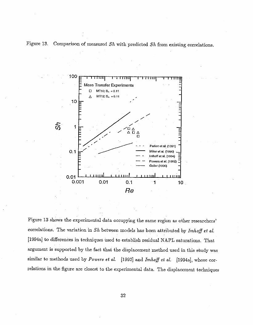
Figure 13, Comparison of measured Sh with predicted Sh from existing correlations.
100
10
0.1
0.01 0. 001 0.01 0.1 1 10
Re
Figure 13 shows the experimental data occupying the same region as other researchers’
correlations. The variation in Sh between models has been attributed by Imho$ e t al.
[1994a] to differences in techniques used to establish residual NAPL saturations. That
argument is supported by the fact that the displacement method used in this study was
similar to methods used by Powers e t al. [1994a], whose cor- [1992] and Imho$ e t al.
relations in the figure are closest to the experimental data. The displacement techniques
32

d .rl
b n,
M O z z W z 0 Od
S ? 3 0
co z 0
n E!
2- %?
V
0
33

were intended to imitate the NAPL-emplacement processes occurring in real groundwa-
ter systems. In contrast, Parker e t al. [1991] and Miller e t al. [1990] stirred NAPL
with their porous media to create NAPL residual, possibly creating smaller, more spher-
ical NAPL blobs ( P o w e r s e t al., 1992). The technique used by Gekber [1990] resem-
bled the displacement methods except that residual NAPL occupied only a part of the
porous medium in her experiments. Consequently, her work required a complex, multi-
dimensional method of analysis to account for lower dissolution rates (Imhofl e t aZ.,
1994a).
Also apparent in Figure 13 is a discrepancy in the trend of data from this study and
that from other investigations. Sh decreases with increasing R e in this study, but in-
creases with increasing Re in other studies. The reason for the opposing trends is found
in Sh. None of the existing models was based on temperature-variant data, so variations
in Sh are due prim&ly to KI. For data from this investigation, Sh is controlled not
only by Kr, which increases by about loo%, but also by D,, which increases by 162%
over the temperature range used in the experiments. In the isothermal models repre-
sented in the figure, D, is constant, or varies only slightly with different compounds.
The diffusivity is a key factor in theoretical models of interfacial mass transfer. Mass
transfer by diffusion done is represented by the stagnant film model, in which the mass
transfer coefficient is directly proportional to diffusivity, whereas models incorporating
advective as well as diffusive processes predict that Kl is proportional to D, to a power
less than one, frequently 0.5. In dimensionless form, these translate to Sh cc 5’cO.O for
purely diffusional mass transfer, and Sh 0; SCO.~ for combined diffusion and advective
processes.
34

Miller e t al. [1990] included Scon5 in their model, advocating the combined effects of
advective and diffusive transport, but their use of relatively D,-invariant data precluded
its validation. As was seen in Figure 8, the variation in D m with temperature can be
substantial: between 5°C and 40°C, D m decreases by 83%.
Given the sensitivity of the data from this study to D m , a more appropriate compari-
son to existing correlations would include Sc. In Figure 14, the model predictions are
modified by SC' .~ , b'ased on the estimated D m values given in Table 5. The trends of
the experimental data are brought into closer agreement with previous works, suggesting
that Sh is a function of Sc. The contrasting trends of Figures 13 and 14 indicate that
the exponent of Sc is probably close to 0.5.
In order to determine the relationship between Sh and Sc, a dimensionless model was fit
to the experimental data. Because of the small number of data, the number of fitted pa-
rameters was kept to a minimum, and only the simplest power-law form was considered.
The model employed was of the form used by Miller e t al. [1990]:
where p ' s are parameters to be estimated or fitted, and Sh* = K;d,/D,. Since the two
media types were similar in size and because of the uncertain quality of the sand results,
additional measures of media geometry, such as those used by Geller [1990] and Powers
e t al. [1992], were not of primary relevance to this study. Similarly, since transient dis-
solution and dissolution fronts were not pertinent to this study, initial NAPL conditions
35

Figure 14, Comparison of measured S ~ / S C O * ~ with predicted Sh/Sc0p5 from existing cor- relations.
Re
used by Gebker [1990] and the x f / d , grouping used by Imho$ e t al.
included.
[1994a] were not
Fixed values for exponents and pz were chosen, based on their counterparts in the
existing models, so that only the remaining two parameters were fitted. The software
36

package SYSTAT [1988] was used to fit 60 and p 3 , using both linear and nonlinear re-
gression. Linear regression was used by first linearizing (6) with a logarithmic trans-
formation. Because of uncertainty in the quality of data using the Camp Lejeune sand,
only the twelve measured Kf from the glass bead experiments were used. In both re-
gression analyses the squared residual for each data point was weighted with its esti-
mated standard deviation in the least squares regression.
Results of the model analyses are summarized in Tables 6 and 7. Most values for 6 3 lie
between 0.4 and 0.8. Using R2 as a measure of the quality of the fit, the data are best
approximated with the highest exponents on R e (0.75) and 0, (1.0). However, any com-
bination of specified parameters produces an acceptable fit. Recognizing the limits of
the data set (a small number of data and limited replicates), it makes sense to choose a
model on the basis of preferred values for p1 and ,&, rather than on statistical superior-
ity alone.
An exponent of ,& = 0.75 was selected for Re, both because of the good regression re-
sults and for its agreement with other researchers. Both Mibber e t al.
e t ab. [1994a] proposed this or a similar value. Powers e t ab.
exponent of 0.736 for Re when Sh was posed as a function of only Re and 8, (not their
[1990] and h h o $
[1992] found a best-fit
preferred model).
For ,&, a value of 0.9 was chosen. Again, this value brought good results in regression
analysis and has some support in the literature. A similar value of 0.87 appears in the
model by Imhoff e t ab. [1994a]; Powers e t al. [1994], in a transient dissolution model,
found optimal values for the 8, exponent ranging from 0.750 to 0.960, depending on
porous media characteristics. Although the experimental data of this study were from
steady-state experiments, the lower NAPL saturation levels represented in half of the
. 1 37

Table 6. Results of nonlinear regression.
Specified Parameters
P1 0.33
0.50
0.60
0.75
P 3
0.44 0.60 0.90 1.00 0.44 0.60 0.90 1 .oo
': 0.44 0.60 0.90 1.00 0.44 0.60 0.90 1.00
Fitted Parameters with 95% Confidence Intervals
P O
0.26 f 0.87 4.61 f 5.76 10.05 f 7.17 12.93 4 8,35 2.33 f 3.68 3.59 f 4.24 7.80 f 5.38 10.03 f 6.47 2.02 f 3.09 3.10 f 3.54 6.72 f 4.57 8.63 f 5.60 1.62 f 2.37 2.48 f 2.70 5.37 f 3.59 6.89 f 4.53
P 3
0.60 =t 0.52 0.29 f 0.17 0.28 f 0.10 0.28 f 0.09 0.37 f 0.21 0.36 f 0.16 0.36 f 0.09 0.36 f 0.09 0.41 f 0.21 0.41 f 0.16 0.41 f 0.09 0.41 f 0.09 0.48 f 0.20 0.48 f 0.15 0.48 f 0.09 0.48 f 0.09
Adjusted R2
0.899 0.968 0.989 0.991 0.950 0.972 0.990 0.991 0.953 0.973 0.990 0.991 0.957 0.976 0.991 0.991
data set were established by dissolution of a higher initial saturation. Consequently, the
NAPL saturation element of the transient dissolution correlation is relevant to this work. ,
With the chosen values of p1 and P 2 , the regression results for the nonlinear fit (with
95% confidence intervals) are
P o = 5.369 f 3.594
P 2 = 0.479 f 0.091 (7)
38

Table 7. Results of linear regression.
Specified Parameters
PI
0.33
0.50
0.60
0.75
P 3
0.44 0.60 0.90 1 .oo 0.44 0.60 0.90 1 .oo 0.44 0.60 0.90 1 .oo 0.44 0.60 0.90 1 .oo
Fitted Parameters with 95% Confidence Intervals
~~
W O )
0.79 f 2.11 1.23 f 1.69 2.06 f 1.08 2.34 f 0.97 0.54 f 2.03 0.99 f 1.62 1.82 f 1.04 2.09 f 0.96 0.40 f 1.98 0.84 f 1.58 1.67 f 1.02 1.95 f 0.95 0.18 f 1.91 0.62 f 1.51 1.45 f 0.99 1.73 & 0.95
P 3
0.31 f 0.29 0.31 f 0.23 0.31 f 0.15 0.31 f 0.13 0.39 f 0.28 0.39 f 0.22 0.39 f 0.14 0.39 f 0.13 0.44 f 0.27 0.44 f 0.22 0.44 f 0.14 0.44 f 0.13 0.51 f 0.26 0.51 f 0.21 0.51 f 0.14 0.51 f 0.13
Using linear regression on the transformed model
Po = 1.455 f 0.995
,f?z = 0.506 f 0.137
Adjusted R2
0.989 0.995 0.999 0.999 0.992 0.996 0.999 0.999 0.993 0.996 0.999 0.999 0.994 0.997 0.999 0.999
Of the two models, the nonlinear form is slightly more robust: although the R2 value
is slightly lower, confidence intervals are narrower for the nonlinear than for linear re-
39

gression. The normal probability plots of the standardized residuals are reasonably lin-
Property Change
Density (water) -1% Density (PCE) -3% Viscosity (water) -57% Viscosity (PCE) -31% Diffusivity (PCE in water) +162% Interfacial tension 33% Solubility (PCE in water) -2%
em for both cases, so neither approach can be invalidated on that basis. In either case,
model analysis predicts an exponent for Sc of approximately 0.5 for the glass bead ex-
periment s.
Source
AIChE [1985] AIChE [1985] AIChE [1985] AIChE [1985]
Tyn and Calus [1975] measured measured
1.4 Discussion
1.4.1 Physical and Chemical Properties
The effect of temperature variation between 5°C and 40°C on physical and chemical
properties of PCE was determined by laboratory investigation and from an examination
of the scientific literature. These results are summarized in Table 8.
Over the range of temperatures studied, the viscosity and diffusivity were the only prop-
erties which were significantly affected. The viscosity of both water and PCE decreased
by 57% and 31% respectively, while the molecular diffusivity of PCE in water increased
40

by 162%. These properties affected the rate of mass transfer as was demonstrated in
the effect of temperature on the mass transfer rate coefficient. However, because tem-
perature over this range did not significantly alter the PCE/water interfacial tension,
mobilization of residual PCE droplets due to increases in water temperature was not ex-
pected.
1.4.2 Mobilization
The mobility of trapped PCE droplets is dependent upon interfacial, viscous and grav-
itational or buoyancy forces. Interfacial forces act to trap droplets within the porous
structure, while viscous and gravitational forces act to mobilize droplets in the direc-
tion of the groundwater velocity (viscous) or gravity (buoyancy for heavier-than-water
droplets). To assess the importance of these forces on mobilization, investigators com-
monly examine two dimensionless groupings: the Capillary nurnber, Ca = 'u,p,/o,,, the
ratio of viscous to interfacial forces; and the Bond number, Bo = ( p , - p,)gc$/4o,,, the
ratio of gravity to interfacial forces. Here, va is the pore-water velocity of the aqueous
phase, Q,, is the IFT between the nonaqueous and aqueous phases, pn and Pa are the
nonaqueous and aqueous-phase densities, g is the gravitational acceleration, and dp is
a representative grain diameter for the porous medium. Mobilization of residual NAPL
may occur if Ca and/or Bo are increased above critical values.
Based upon the changes in physical properties associated with temperature changes be-
tween 5°C and 40"C, neither of these dimensionless numbers will be changed signifi-
cantly. For this reason, pumping heated water within a PCE-contaminated aquifer is
not expected to mobilize PCE residual. This conclusion is consistent with observations
in the mass transfer experiments, where no PCE droplets were observed to mobilize from
the column.
I 41

1.4.3 Dissolution
Over the temperature range from 5°C to 40°C, the heated water had a very small ef-
fect on the solubility limit of PCE in the aqueous phase, but a significant effect on the
rate of PCE dissolution. The measured mass transfer rate coefficients were within the
range of values predicted from existing correlations. However, to correctly account for
the trend of Sh* with Re, it was necessary to include Sc in the mass transfer model: the
diffusivity of PCE in water is significantly affected by temperature, and with the excep-
tion of the correlation of Miller e t al. 119901 other models assumed a linear dependence
of K,* on D,, From this study it was determined that for dissolution of residual PCE
Sh* is proportional to ScO.', which is equivalent to 0: Dg5.
The maximum potential enhancement of PCE dissolution due to heated water is illus-
trated by examining the maximum potential mass flux, KTC,, as a function of tem-
perature. (Actual mass flux per unit aqueous-phase volume of the porous medium is
K,*(C, - C). The maximum potential mass flux is an upper bound.) The maximum
potential mass flux is plotted versus temperature in Figure 15, where K; was estimated
from equations (6) and (7), and C, taken from measured solubilities. The mass flux in-
creases by a factor of two as the temperature increases from 5°C to 60°C. This improve-
ment in the mass flux is due primarily to the increase in K;. This increase is not large,
and in many situations may not be justified given the added expense of heating water.
However, for other NAPLs where C, is more significantly affected by temperature hot
water flooding may still be an effective technology.
42

Figure 15. Maximum potential mass flux of PCE for representative conditions using equations (6) and (7).
60
om Q- 20
0
I I I I
/ wa= 1 m/day
e = 0.04
0 20 40 60
Temperature (" C)
43

2 Alcohol Flushing
2.1 Background
2.1.1 Introduction
Recently, it has been suggested that surfactants, alcohols, and mixtures of these chem-
icals may be effective for in situ treatment of aquifers contaminated with hazardous or-
ganic compounds. These technologies 'were originally developed in the petroleum indus-
try, and several reviews have been written on this work (Reed and Bealy , 1977; Lake,
1983). To set the background for this investigation, the literature on alcohol flooding in
the petroleum industry is reviewed below. This is followed by a review of the work to
date using alcohol flooding for remediation of contaminated aquifers.
2.1.2 Alcohol Flooding - for Enhanced Oil Recovery
The interest in miscible alcohol flooding in the oil industry increased after the appear-
ance of papers by Pausell E19531 and Gat l in and Slobod [1960]. These authors found in
a series of laboratory experiments that recovery of oil displaced by concentrated alcohol
solutions was close to 100%. Gat l in and Slobbod [1960], Tuber e t al.
and Csaszar [1962] obtained oil recovery rates close to 100% for naphtha, Soltrol, and
Kendx in sand columns, using iso-propanol alone or a combination of methanol with ei-
119611 and Rolm
ther iso-propanol or n-butanol.
44

Tuber et ul.
was probably impractical because of the high cost of alcohols and the relatively large
moun t of alcohol necessary for significant improvement in oil recovery. In this research,
Tuber et al.
in a nearly piston-like fashion. This investigation used iso-propanol (IPA) and tertiary
butyl alcohol (TBA). The authors studied equilibrium phase behavior for two ternary
systems: IPA/Brine/Soltrol and TBA/Brine/Soltrol. It was shown that an essential first
step in any investigation of alcohol flooding is the determination of the phase diagram,
complete with tie lines and plait point. As a result of the study of phase behavior for
these two systems, Taber et al. [1961] predicted and then experimentally demonstrated
that two kinds of alcohol displacement exist. In the first type (TBA/Brine/Soltrol), the
nonaqueous (or oil) phase dominates as miscibility is approached and, therefore, remains
continuous throughout the flood. In the second type, the aqueous phase dominates as
miscibility is approached; therefore, the nonaqueous phase passes through a residual sat-
[1961] ‘reported that the commercial application of alcohol-slug processes
[1961] defined the essential characteristics of a system of slugs behaving
uration state before miscibility is achieved. The behavior of these kinds of systems is
characterized by a plait point location on the binodal curve. The following relationships
were also studied: recovery versus alcohol slug size, recovery versus initial oil satura-
tion, phase viscosity versus alcohol concentration, and relative penneabilities of stabi-
lized banks. d
Several researchers have attempted to simulate alcohol flooding ( Wuchman, 1963; Dono-
hue, 1963). The experimentally determined phase behavior effects were incorporated
into numerical models developed by these authors. The following conclusions were drawn
on the basis of these studies: (1) It is possible to simulate the basic features of alcohol
displacement in porous media by means of suitably designed numerical models; (2) A
theoretically sound method of selecting the immovable oil and water fractions is to base
45

these upon the relative permeability data; (3) Numerical models can more closely repro-
duce experiment al data when they incorporate nonequilibrium effect s.
In the field of physical chemistry, research has shown that alcohols can dissolve signifi-
cant quantities of oil in water ( D e Visser e t al., 1977 Knickerboker e t al., 1979). How-
ever, this process is not efficient in dissolving heavier oils (Bellocq e t al., 1981). Alco-
hols with longer chains, such as butanol, pentanol, or hexanol, are more effective, but
less soluble in water. To solubilize these heavier oils, a surfactant must be added (Rouz-
Desgranges et al., 1981).
&arson e t al. [1982] formulated the primary mechanisms of residual oil recovery by al-
cohol flooding. These mechanisms include solubilization, interfacial tension (IFT) reduc-
tion, and swelling of the nonaqueous phase. As the rate of solubilization or dissolution
of oil into the aqueous phase increases, oil can be produced in the aqueous phase. The
most effective mode for oil recovery is the achievement of complete miscibility. In prac-
tice, this condition is difficult to achieve using a finite volume alcohol slug, since the dis-
persive mixing at the alcohol front may dilute alcohol to a lower concentration, and the
alcohol slug may disappear with travel distance. In the two-phase flow region, increasing
alcohol concentration leads to a decrease of IFT between the aqueous and nonaqueous
phases. This reduction in IFT causes an improvement of the displacement process or oil
mobilization. Tuber 119691 stated that swelling of oil interacting with alcohol is one of
the main mechanisms contributing to enhanced oil recovery. Swelling occurs when the
alcohol preferentially partitions into the oil phase rather than into water. In general,
higher molecular weight alcohols tend to partition preferentially into the oil phase (Tuber
et al., 1961; Holm and Csaszar, 1962, Lam e t al., 1983). As the oil phase swells it be-
comes easier to displace and may mobilize.
46

Lam et ab.
rium and nonequilibriurn conditions. An oil globule is displaced when the IFT is reduced
[1983] studied mobilization of residual oil by an alcohol slug under equilib-
to an extent that the pressure gradient created by motion of the continuous phase is suf-
ficient to overcome the capillary forces holding the globule in place (Tuber, 1969; Mel-
rose and Brandner, 1974; Abrums, 1975). Two different classes of experiments were
performed by Lum e t al. [1983] to determine the sensitivity of swollen residual oil dis-
placement to the capillary number. The oil globules had been swollen by mass transfer
from a continuous phase flowing too slowly to displace the drop. A set of experiments
was performed on an oil drop that initially contained 15 wt% of n-propanol and some
water, with the oil phase composition on the binodal curve. Surprisingly, slightly swollen
globules required a larger capillary number for mobilization than the original droplet.
Thus, the capillary number required for mobilization can go through maximum as the
volume of the oil droplet increases, due to the complexity of pore and globule geometry.
A small increase in the volume of a residual oil globule disconnected from other adjacent
drops is likely to make the drop more difficult to mobilize; however, large increases in
swollen globule volume (greater than 15%) will tend to increase the mobility of the glob-
ule, making it much easier to displace. The last statement is very important for practi-
cal applications, since it indicates a threshold value for the amount of alcohol required
for efficient oil recovery. 1
2.1.3 Remediation of Contaminated Aquifers by Alcohol Flooding
Removal of residual NAPLs from contaminated ground waters 'is in many ways analo-
gous to oil recovery from subsurface reservoirs. The effects of solubilization, IFT reduc-
tion, and NAPL swelling can be examined using similar techniques.
47

It is well recognized that the nature of the solvent has an impact on the solubility of or-
ganic contaminants (Yalkowsky, 1986; Gupte and Dunner, 1987; Pinal et al., 1990).
These authors have investigated the theoretical and experimental aspects of alcohol co-
solvency on hydrophobic organic chemical solubility. It has been shown that increas-
ing the alcohol volume fraction in water/alcohol systems increases hydrophobic organic
chemical solubility in an essentially log-linear manner. Several theoretical approaches
have become available over the past decade for dealing with oily contaminant solubil-
ity in solvent mixtures. Among these are the following: the UNIQUAC/UNIFAC mod-
els (fiedenslund et al., 1975; Prausnita et al., 1980), the log-linear model ( YuZkowsky
1986), and the three-sufi equation method (Williams and Amidon, 1984). Application
of the solubility parameter theory to mixed solvents was discussed in a review by Barton
[1975]. The results of these investigations showed the possible approaches for choosing
the most effective combination of alcohols for different mixtures of contaminants (Pinal
et al., 1990).
Zenon El9861 studied the feasibility of in situ alcohol treatment for hydrocarbon con-
taminated soils. Zenon I19861 used short-chain alcohols (methanol, ethanol, iso-propanol)
to increase the dissolution of 1,2,3-trichlorobenzene (TCB) in water. Concentrations as
high as 30% to 50% alcohol were required to increase TCB solubility by a factor of ten
or more, Iso-propanol was found to be more efficient than ethanol or methanol.
The authors of recent experimental investigations (Boyd , 1991; Brandes, 1992; Put-
WaTdhan, 1992; Brundes and Parley, 1993) concluded that alcohol flooding was a promis-
ing technology for removing residual NAPLs from ground water. These researchers con-
ducted a set of laboratory experiments at 23°C with isopropyl (IPA), and tert-butanol
(TBA) alcohols, and with the NAPLs trichloroethylene (TCE) and tetrachloroethylene
48

(PCE). Ternary phase diagrams were determined experimentally for the following sys-
tems: (1) IPA/TCE/water, (2) TBA/TCE/water, and (3) TBA/PCE/water. A ternary
diagram for the system IPA/PCE/water was estimated by the UNIFAC method. The
IFT of these systems were estimated using the method developed by Fu et ul. [1986].
The water and alcohol flooding experiments were conducted to evaluate the effective-
ness of using different alcohols at different concentrations. Based on their experimental
results, Bran& and Furley I19931 concluded the following: (1) 100% recovery of resid-
ual TCE can be achieved by using one pore volume of a solution of 70% (by volume)
TBA or IPA and 30% water. (2) Use of IPA for displacement of residual PCE is ineffec-
tive. Relatively effective removal of PCE ( 90% recovery) can be accomplished using one
pore volume of a solution of 70% (by volume) TBA and 30% water. (3) The cause of the
more effective displacement of residual NAPL by TBA is the preferential partitioning of
this alcohol into the nonaqueous phase. The swelling of the NAPL phase leads to the
formation of a high saturation NAPL bank. (4) The experimental data demonstrated
significant reduction in NAPL phase density for long chain alcohols such as TBA. ( 5 ) All
experimental results are consistent with predictions based on analysis of the correspond-
ing ternary diagrams.
1
2.1.4 Summary
The review of experimental data presented above demonstrates that alcohol flooding is a
complex process which includes mass transfer and alteration of physico-chemical proper-
ties of nonaqueous and aqueous phases. Although many features of this process are now
known, significant questions remain. These include: Where NAPL and aqueous pha-
ses remain immiscible during an alcohol flood, what effect does the alcohol have on the
49

rate of NAPL dissolution? Is mobilization of NAPL residual during an alcohol flood pre-
dictable in real porous media, where the soil structure may be complex and the distri-
bution of NAPL residual nonuniform? Given the importance of ternary phase diagrams
for representing the behavior of NAPL/water/alcohol systems and the effort required in
measuring them experimentally, how accurate are predictive methods? The intent of this
investigation was to address each of these questions.
2.2 Experimental Methods
5
2.2.1 Overview
To investigate alcohol flooding on enhanced aquifer remediation, the PCE/methanol/
water system was selected for study. The importance of PCE as a groundwater contam-
inant was discussed earlier. Methanol was chosen as a representative alcohol because
(1) it is relatively inexpensive, (2) once diluted to small concentrations in groundwater
it is readily biodegradable, and (3) it is representative of a class of alcohols which do
not significantly partition into NAPLs and thus will not enhance NAPL migration due
to swelling of NAPL droplets. Because of the potential difficulty in controlling NAPL
movement in the subsurface (e.g., denser than water NAPLs may sink to lower regions of
the aquifer) alcohols which do not enhance NAPL mobility are preferred in some situa-
tions.
The experimental study began with an examination of the effect of a select range of
methanol/water volumetric fractions (O'%, 20%, 40%, and 60% 'methanol by volume) on
the system behavior: phase equilibria, phase density, and interfacial tension. A ternary
50

phase diagram was generated from the experimental data, and then compared with the-
oretical predictions. With the physical and chemical properties from these experiments
coupled with existidg data for viscosity and molecular diffusivity from the literature, the
system was well-characterized. Finally, a column experiment was performed to measure
the effect of a methanol/water mixture on the dissolution and mobilization of residual
PCE in a porous medium. Analysis of data from this experiment made use of the physi-
cal and chemical properties measured earlier.
2.2.2 Materials
All chemicals were HPLC grade and were used without further purification. Alcohols
were purchased from Fisher Scientific, and PCE from Aldrich Chemical Company. Wa-
ter was deionized and distilled in our laboratory as described earlier. Hydranal-Coxdomat/
CG cathode solution and Hydrand-Coulomat/AG anode solution for Karl Fischer titra-
tions were purchased from Reidel-deHaen through Fisher Scientific.
All glassware was washed with Alconox laboratory detergent and tap water, rinsed with
tap water, soaked overnight in 1.0 N HCI solution, rinsed thoroughly (at least three
times) with tap, followed by deionized, distilled water, and oven-dried at 102-105°C.
Glassware used in experimental measurements of interfacial tension was submerged over-
night in a warm solution of dichromate in sulfuric acid, rinsed thoroughly with tap, fol-
lowed by deionized, distilled water, and drip-dried on clean filter paper in a reasonably
dust-free environment, as per ASTM Designation D 971-91 (ASTM, 1991).
All liquid measurements were made using volumetric pipets, volumetric flasks, or Hamil-
ton Gas-tight syringes, depending on the volume desired.
51

2.2.3 Eauilibrium Phase Partitioning: Generator Columns
In order to describe the equilibrium conditions of a PCE/methanol/water system, it is
necessary to measure the equilibrium concentrations of PCE, water and methanol in
both the nonaqueous and aqueous phases. Two different experimental techniques were
used to create nonaqueous-aqueous phase solutions which were in equilibrium: batch-
contacting experiments and experiments using generator columns.
Liquid-liquid equilibria have traditionally been achieved by bat ch-contacting. Fixed vol-
umes of solute and solvent are combined in a flask or mixing vessel and shaken (shake-
flask batch) or magnetically stirred (stir-flask batch) at a controlled temperature. The
equilibration period is typically followed by a stabilization period during which solute
particulates or colloidal dispersions are separated out of the bulk solvent phase, which
is then sampled and analyzed by an appropriate technique. Mutual solubilities may be
determined by sampling both equilibrated phases of a binary mixture.
Discrepancies in published solubility data illustrate problems with bat ch-contacting tech-
niques, particularly when the goal is to saturate water with a hydrophobic organic com-
pound. Because many organic compounds are only sparingly soluble in water, their con-
centrations may be drastically affected by colloidal or particulate suspensions, by losses
due to solute volatilization, and by adherence to the surfaces of transfer vessels. Mi-
croemulsion formation may be promoted by turbulent mixing practices typically em-
ployed in shake-flask batch methods to enhance mass transfer. More gentle contacting
by slow stirring may reduce (but not necessarily eliminate) emulsification, but only at
the expense of expediency: Equilibration periods as long as several weeks are not un-
common (Barrie Webster e t al., 1989). Extended mixing periods may increase the po-
tential for volatilization losses. In addition, several replicates over time are necessary
52

to confirm equilibrium. Batch results obtained even by the same researchers confirm
the dependence of solubility data on experimental conditions including the methods of
equilibration (vigorous shaking or gentle stirring) and solvent-excess solute separation
(gravity-settling, filtration, or centrifugation) (Bharath e t ak., 1984). Solubility data are
also sensitive to variations within a given method (equilibration time, settling time, filter
pore size, centrifugation speed, etc.).
Continuous flow-through methods resolve many of the problems associated with batch
techniques. A solid support with a large surface mea such as glass beads, diatomaceous
silica, or a chromatographic media, is coated with the analyte and packed into a column.
The solvent flows through the column, is dispersed through the packed bed, and contacts
the solute at a rate sufficiently slow to prohibit emulsion formation and ensure liquid-
liquid equilibrium. The large solute-solvent interfacial area within the porous bed pro-
motes rapid equilibration even at moderate flow rates.
The generator column technique is a continuous flow-through process introduced in the
1970s (Veith a n d Coms tock , 1975). Recently, it has become the preferred method for
the aqueous dissolution of hydrophobic chemicals (May e t al., 1978; D e V o e e t al., 1981;
Wusik: e t al., 1983; Bi l l i ng ton e t al., 1987) and has also been applied to measurements
of vapor pressure and octanol/water partition coefficients ( D e V o e e t al,, 1981; Wasik e t
al., 1983).
The advantages of generator columns over batch methods for preparing aqueous solu-
tions saturated with hydrophobic organic compounds are presented in detail in the lit-
erature (May e t al., 1978; D e V o e e t al., 1981; Wasik e t al., 1983; Bi l l ing ton e t al.,
1987). These include
1. equilibration is rapid;
53

2. colloidal or particulate suspensions are absent;
3. exposure to the atmosphere is minimized;
4. column surfaces become equilibrated with the saturated solution, minimizing ad-
sorption;
5 . large volumes of saturated solutions can be generated continuously;
6. analyte requirements and waste generation are minimal;
7. the necessary equipment is inexpensive and readily available;
8. columns are reusable; the support can even be cleaned and coated with a different
analyt e;
9. columns may be placed in series, either to confirm equilibrium using a single solute,
or to equilibrate a particular solvent with a number of analytes; and
10. once the apparatus is assembled, varying external parameters such as temperature,
flow rate, or the composition of the feed solution is a simple task.
PCE aqueous solubility was measured by the continuous flow-through generator columns
at 20°C. The techniques employed for the generator columns were in accordance with
those published by the National Bureau of Standards (DeVoe e t al., 1981) with a few
minor modifications. 5-ml borosilicate volumetric pipets served as the generator columns.
Each pipet consisted of two sections 6.0 mm in outside diameter connected by an en-
larged bulb section, with an outside diameter of approximately 9.0 mm. The volumetric
pipets were shortened such that the total column length was approximately 25 cm. The
54

section with a 6.0-mm outside diameter located below the bulb section was packed with
120/140 mesh glass beads manufactured by Cataphote, Inc. The beads, held in place by
glass wool plugs, provided an inert support for the stationary NAPL phase, 12-15 cm in
length.
The pipets, glass beads, and glass wool plugs were silanized to deactivate all internal
column surfaces by pre-treating with Glass-Treat, a silanizing agent manufactured by
Alltech Associates containing dimet hyl-dichloro-silane. The surfaces were then rinsed
with anhydrous methyl alcohol purchased from Fisher Scientific, and air-dried under a 1
chemical fume hood. The ends of the columns were wrapped with Teflon tape and fit-
ted with Teflon ferrules and stainless steel Swagelock fittings. The upper (outlet) end
of one column was connected to the lower (inlet) end of the second column with a Z-
shaped section of stainless steel tubing, approximately 35 cm in length. The tubing was
seated with stainless steel ferrules into the Swagelock fittings at the column ends. Stain-
less steel tubing connected the outlet of the second column to a stoppered 500-ml vac-
uum flask, vented to a carbon trap to collect fluid waste and harmful vapors. The com-
bined pore volume of two generator columns in series was estimated to be in the range of
2.5 ml. Figure 16 is a schematic of the generator column setup.
Because PCE solubility is expected to increase markedly in more concentrated cosolvent
mixtures, two larger packed coh"s were added in front of the generator columns to
provide adequate PCE for dissolution for cosolvent mixtures with large methanol/water
fractions. The columns, manufactured by Ace Glass Co., Inc., were each 50 ml in vol-
ume, threaded at both ends, and supplied with screw-in end caps and Teflon frits with
glass plate inserts. The large columns were packed wet under PCE by pumping in PCE
upflow from a Harvard Apparatus Infusion-22 syringe pump equipped with a Hamilton
100-ml Gastight syringe, while pouring 120/140 mesh glass beads through a funnel at
55

Figure 16. Experimental setup using generator columns
Glass columns packed with glass beads, PCE, and water
Sample port #l
to waste
C U \ I Pipets packed with
Syringe Pump glass beads, PCE, and water (Generator Columns) [water and methanol solution)
the top of the column. After packing and loading with PCE, the columns were flushed
by pumping water down-flow through the column, pushing out a front of dense, free
phase PCE, and leaving the packed bed residually saturated with PCE. Teflon tubing
was used to connect the columns in series and to flow solvent, supplied by a Hamilton
Gastight 100-ml glass syringe through the system.
The solvent used in the generator column experiments consisted of aqueous mixtures of
methanol, including O%, 20%, 40%, and 60% methanol by volume. The flow rate was
maintained between 0.5 and 1.0 ml per minute. Preliminary experiments confirmed that
flow rate had no significant effect on the results within the range of flow rates employed.
The effluent reservoir was maintained at an elevation such that pressures within the
columns were always above atmospheric. Samples were extracted from the efffuent of
56

the generator columns. Two of the nuts in the Swagelock crosses at the top of each gen-
erator column were fitted with Teflon-lined silicone septa and used as sampling ports.
Hamilton 1-ml Gastight syringes were used to collect several 1-ml samples, alternat-
ing between the two generator columns in series. The samples were filtered with a 0.2-
pm nylon syringe filter housed in a stainless steel Fisher Scientific syringe holder. The
samples were immediately diluted into 9 ml of isopropanol, dispensed earlier into pre-
weighed 11.1-ml borosilicate screw-top vials. The diluted samples were then dispensed
into Hewlett Packard 2-ml autosampler vials and crimp-sealed until analysis by gas chro-
matography. Samples were analyzed using the same equipment and procedures as were
employed when analyzing bat ch-equilibrated samples.
Nonfiltered samples were also collected and analyzed during preliminary experiments,
PCE concentrations from samples collected using the two techniques did not differ in a
statistically significant manner, indicating that there were a minimal number of colloidal
particles larger than 0.2 pm in solution. Data reported below are only from filtered sam-
ples.
2.2.4 Equilibrium Phase Partitioning: Batch Experiments
Because it was impossible to sample the nonaqueous phase in generator column exper-
iments, batch experiments were also performed to measure equilibrium concentrations
of PCE, water and methanol in both nonaqueous and aqueous phases. Equal volumes
(approximately 30 ml each) of PCE and aqueous solutions of methanol, including 0%,
20%, 40%, 60% percent methanol by volume, were batch-equilibrated by the shake-flask
method in 50-ml Erlenmeyer flasks at 20°C. Two batch flasks were prepared at each
57

methanol/water fraction. The flasks were continuously shaken on a Junior Orbital Au-
toshaker at 100 revolutions per minute (rpm), with periodic inversion and vigorous shak-
ing by hand for a minimum of 12 hours before sampling. To minimize leakage and volatile
losses, the flasks were completely filled and sealed with threaded screw-caps wrapped
with Teflon tape.
In order to maintain the aqueous phase at a known methanol concentration, the aqueous
phases were periodically replaced with fresh methanol/water solutions. Equilibrium was
confirmed by at least two consecutive measurements of PCE in the aqueous phase over
time that agreed within experimental error.
2.2.4.1 Sample Collect ion and Dilut ion
from the shaker, inverted, and the phases allowed to separate until no turbidity was ob-
served in either phase. The flasks were then vented by puncturing the Teflon-lined sil-
icone septa with U-shaped sections of stainless steel tubing, approximately 1.6 mm in-
ternal diameter and 300 mm in length, to equalize pressure during sampling. Ten 1-ml
Before sampling, the flasks were removed
samples of the nonaqueous phase were first withdrawn from each flask using 1-ml Hamil-
ton Gas-tight syringes and diluted into 9-ml of isopropanol (IPA) in 11.1-ml borosilicate
vials with open-top screw caps and Teflon-lined silicone septa. These samples were used
to determine the methanol concentration in the nonaqueous phase.
5-ml Hamilton Gas-tight syringes were then used to collect 5-ml samples of each aqueous
phase, which were filtered with a 0.2-pm nylon syringe filter housed in a stainless steel
Fisher Scientific syringe holder. Samples were filtered to remove colloidal or particu-
late suspensions, which may have resulted during batch contacting. The filtered samples
were diluted into 5-ml of IPA in 11.1-ml borosilicate vials. The aqueous phase samples
were used to determine the PCE and methanol concentration within the aqueous phase.
58

The flasks were refilled by topping off with fresh methanol/water solutions, the septa
were replaced, and the flasks resealed and returned to the shaker for future sampling.
Pasteur pipets were used to quickly dispense the diluted samples of each phase into 2-
ml Hewlett Packard GC autosampler vials, which were crimp-sealed with minimal head
space to minimize volatility losses before analysis.
A second set of samples was collected from the nonaqueous phase of each flask for deter-
mination of the water content. At least five 1-ml samples of the nonaqueous phase were
extracted from each flask using 1-ml Hamilton Gas-tight syringes. Sample masses were
determined by weighing the syringe immediately before and after sampling. Nonaqueous
phase samples batch-equilibrated with methanol/water mixtures were also transported
to a Hoechst Celanese Reidel-deHaen Laboratory for independent analysis of water con-
tent.
,!?.2.4.,!? Gas Chromatoqraphic Analusis
matograph with Hewlett Packard 7673A Automatic Sampler Tower and HPChem Sta-
tion were used to determine PCE and methanol concentrations within the aqueous and
nonaqueous phase samples. The gas chromatograph was equipped with a Flame Ioniza-
tion Detector (FID) and a Supelco Carbopack 3% SP 1500 packed column, 80/120 mesh,
3.2-mm internal diameter and 304.8 cm in length. The flame was maintained by a flow
of 20 PSI hydrogen gas and 36 PSI compressed air. The carrier gas was Helium at ap-
proximately 20 ml/min with Nitrogen as the make-up gas at approximately 10 ml/min
to maintain a total column head pressure of 30-40 PSIG. 1.0-pl samples of the diluted
A Hewlett Packard Model 5890A gas chro-
aqueous or nonaqueous phase samples were automatically injected by the autosampler
with two sample washes, two sample pumps and eight solvent washes of IPA between
samples to eliminate carry-over peaks from previous samples.
59

The temperature program used for sample analysis began with an initial temperature
of 100°C for three minutes to separate the early-eluting alcohols, followed by a ten de-
nute temperature ramp to 190°C. The ramp was then retarded to 1.5 degrees per
minute to a find temperature of 202°C. The final temperature ramp was necessary to
flatten the baseline while the PCE peak emerged.
The HPChem Station permitted post-run manipulation of the data including re-integration
and threshold alterations.
2.2.4.3 Calibration Standards Standards of known concentrations of PCE in meth-
anol/water mixtures and methanol in PCE were used to develop calibration curves from
which sample concentrations were determined. The gas chromatograph peak area was a
linear function of concentration for both PCE and methanol over the entire range of con-
centrations studied. All regressions had R2 values greater than 0.995, with typical values
of greater than 0.999.
The standards were prepared by successive volumetric dilutions of concentrated stock
solutions. The standards were diluted in an identical manner as the samples, and stan-
dards were analyzed periodically during sample analyses. To account for instrument
drift, data from standards bordering each subset of data were combined to evaluate that
subset. Dilution blanks were also used throughout sampling analysis to monitor poten-
tial carry-over due to high concentrations and column overload.
60

2.2.4.4 Karl Fischer Coulometric Titrations A Fischer Coulomatic Titrimeter Model
447 was used to measure the water content of samples collected from the nonaqueous
phase. In the presence of sulfur dioxide, an organic nitrogen base, and an alcohol, wa-
ter was consuxned by a stoichiometric reaction with iodine. The instrument automati-
cally titrated the sample to dryness by generating iodine coulometrically from Karl Fis-
i
cher Hydrmal reagents. At the endpoint, a trace excess of highly conductive free iodine
caused a sharp decrease in cell resistance, detected amperometrically by a dual platinum
electrode. Sample water content was automatically calculated based on the electrical
charge required to produce the iodine needed to complete the titration.
Karl Fischer Titrations were conducted in accordance with ASTM Designation E 203-92
(ASTM, 1992) and the manufacturer’s User’s Manual for the Fisher Coulamatic Titra-
tor Model 447. The, cathode and anode compartment vents were fitted with Drier-Rite
tubes to prevent the intrusion of atmospheric moisture into the otherwise closed titration
vessel.
2.2.5 Equilibrium Phase Partitioning: Titrations
The solubility curve in ternary phase diagrams corresponds to the entire set of combina-
tions of the three components which bounds regions where two phases exist. The use of
ternary phase diagrams for illustrating phase partitioning in three component systems
is described in detail below. The titration method is used to help define points on the
solubility curve.
In the titration method one of the components of a ternary system is added in small in-
crements to a binary mixture containing the remaining two components in separate pha-
61

ses. The titration continues to miscibility defining a ternary composition that represents
a point on the solubility curve (Sayer, 1991). L
A clean, pre-weighed 50-ml Erlenmeyer flask with a threaded, open-top screw cap and
Teflon-lined silicone septum was used as the titration vessel, To minimize volatility losses
and the release of noxious vapors, the vessel remained sealed during the titrations ex-
cept for a small hole punched through the septum through which the tips of the burette
and the volumetric pipets could be inserted. 1.0-ml deionized, distilled water and 0.1-ml
PCE were pipetted into the titration vessel, forming two separate phases. A 10-ml glass
burette accurate to 0.05 ml was inserted into the vessel through the hole in the septum.
The binary mixture was then slowly titrated with methanol until a single miscible phase
formed with no turbidity. The volume of methanol titrated and the final mass of the
vessel were recorded. PCE and water were added in 0.1- and 1.0-ml increments, respec-
tively, to form various binary mixtures which were then titrated with gentle swirling to
miscibility with the cosolvent methanol. Masses were recorded following each addition of
PCE or water and at the titration endpoint. For each titration, the volume of methanol
titrated was recorded.
2.2.6 Phase Densitv
Mass per volume measurements were used to determine equilibrated phase densities.
Following batch equilibration as previously described, ten ml of NAPL were pipetted
into each of seven pre-weighed 10-ml volumetric flasks and their masses recorded. Sam-
ple masses were calculated by difference. This procedure was repeated for each batch-
equilibrated system studied for a total of thirty-five nonaqueous phase samples. A simi-
lar technique was applied to the aqueous phase: Depending on the total volume of PCE-
equilibrated methanol/water remaining after batch equilibration, three to six pre-weighed
62

50-ml volumetric flasks were carefully filled and weighed. Sample masses were deter-
mined by difference. The procedure was repeated for each PCE/methanol/water batch
system studied. ,,
2.2.7 Interfacial Tension
Interfacial tension between the nonaqueous and aqueous phases was measured instanta-
neously and following batch equilibration by the Downward Thrust Ring Method using a
Du Nouy Interfacial Tensiometer CSC No. 70545, in accordance with the manufacturer’s
User’s Manual and ASTM Designation D 971-91 (ASTM, 1991). At least five instanta-
neous and twenty equilibrated measurements were made for each methanol/water frac-
tion studied. The instrument was calibrated against a known weight and its accuracy
confirmed by comphing experimental measurements of the surface tension of water to
values cited in the ASTM Standard Method. The values obtained experimentally fell
well within the acceptable range. The platinum-iridium ring was conditioned by soaking
it in the aqueous-methanol mixture to be tested before introducing it to the sample it-
self. The ring was cleaned between samples by methanol-flaming in the oxidizing portion
of a Bunsen Burner flame.
2.2.8 Mobilization and Dissolution
A series of column experiments were conducted to study the flow and transport pro-
cesses associated with the removal of trapped PCE ganglia by flushing with a methanol/
water mixture. The procedures followed were similar to those developed by Imho$ e t al.
63

[1994a] for a water/trichloroethylene system. These experiments provided data for as-
sessing the effect of the methanol/water mixture on both mobilization and dissolution of
PCE ganglia.
Glass beads identical to those used in the heated water experiments were used as the
porous medium. The column was made of glass and was 27-cm long with a 2.5-cm inter-
nal diameter. A Teflon plunger covered with a fine nylon screen was used at the top of
the column, At the bottom of the column, a similar Teflon plunger was covered with a
coarse stainless steel screen overlaid by a fine Teflon screen, and served as the support-
ing and sealing mechanism. Glass beads were packed underwater by slowly pouring the
beads through a plekiglass tube fitted with a wire mesh screen on one end. The momen-
tum of the falling beads was reduced by the screen before falling through a two to three
centimeter layer of water. Glass beads were added in lifts of approximately five centime-
ters and each lift rodded throughout before additional beads were added.
Once packed with glass beads, the column was mounted and vertically aligned between
an x-ray source and detector used for the nondestructive measurement of porosity and
PCE saturation (McBride and Miller, 1994). Figure 17 presents a schematic of the ex-
perimental setup used in this study. The x-ray source-detector system provided radia-
tion attenuation data used to calculate q5 and S, as a function of vertical location; the
collimated radiation beam was 5 mm by 5 rnm in cross section and provided an average
measurement covering 25% of the horizontal column cross-section at each vertical sarn-
pling location. The random errors associated with these measurements were as follows:
estimated standard error was 0.0018 for q5 and 0.0037 for S,. Measurements of this pre-
cision at a vertical resolution of 5 mm have not been reported to our knowledge for any
cosolvent -enhanced remedi at ion experiments.
64

Figure 17. Schematic of experimental apparatus investigating enhanced remediation with alcohol flushing.
er
Sampling pwt Waste
To permit a visual confirmation of liquid flow through the transparent column walls and
tubing, spectrophotometric grade PCE was mixed with a small amount of dye, oil-red 0,
both purchased from Sigma Chemical Company. The dye permitted visual observations
of PCE mobilization as well as the development of a dissolution front, the region over
which active dissolution was occurring. (Samples of the dyed and pure PCE were pre-
pared and analyzed with gas chromatography and indicated that the dye had negligible
influence on PCE solubility.)
0.9 pore volumes (PV) of PCE, denser than water, was then pumped upwards to achieve
a gravitationally-stable displacement of water from the column. The displacement was
stopped before the invading PCE reached the top of the column. After the injection of
PCE, the flow was reversed and water was pumped downward from the top of the col-
umn. PCE was displaced by 4.1 PV of water at a flow rate of 1.76 m/day followed by
65

an additional 4.9 PV of water at a flow rate of 3 m/day. The disappearance of red PCE
drops from the outflow indicated that displacement of PCE by water was complete and
residual PCE saturation was achieved. After PCE displacement, an x-ray scan of the
column was made to determine the residual PCE saturation along the column.
The methanol/water mixture (60% methanol 40% water by volume) was introduced
through the top of the column with a peristaltic pump. The reappearance of red PCE
drops in the column outflow indicated that a significant amount of PCE was mobilized
and then displaced by the methanol/water solution. The pumping of the methanol/
water solution (approximately 2.1 PV) was continued at a flow rate of 1.76 m/day un-
til red PCE drops disappeared from the outflow. :I
After displacement of the additional amount of separate-phase PCE by the methanol/
water solution, PCE dissolution into the methanol/water mixture becaxne the domi-
nant process during alcohol-enhanced remediation. Because the outflow Teflon tubing
contained sorbed PCE, the tubing was replaced for the solubilization stage of the ex-
periment (Figure 17). To capture the arrival and passage of the PCE dissolution front,
a programmed series of x-ray scans were performed within a subregion of the column.
The number of repeat scans and the length of the subregion were chosen based upon the
analysis of the initial PCE saturation profile and estimates of the dissolution front veloc-
ity assuming equilibrium mass transfer. Effluent liquid samples were collected from the
sampling port (Figure 17) equipped with a three-way valve. Three 0.8-ml samples were
obtained at each sampling time by using a Hamilton gas-tight syringe. Each 0.8-ml was
diluted in 1-mL iso-propanol alcohol and immediately sealed in 2-ml vials.
The samples of the effluent liquid were combined with calibration standards of known
PCE concentration (samples with known concentrations of PCE, methanol, iso-propanol
66

and water) and analyzed by gas chromatography. The same equipment and procedures
used for analysis of aqueous phase samples in the equilibrium phase partitioning experi-
ments were employed here.
2.3 Results
2.3.1 Phase Partitioning
2,8,1 .l PCE Solubilitv in Methanol/ Water Mixtures: Data Data from the gener-
ator columns are described first. Effluent concentrations from both generator columns
were measured through time for the four different methanol/water fractions. As the
aqueous phase flows through the generator columns contacting PCE, phase equilibrium
will be reached: the PCE concentration within the aqueous phase stabilizes and remains
constant through time and space (distance traveled through serial columns). For this
study, equilibrium was considered established when measured PCE concentrations in the
effluent from both columns agreed within experimental error and remained consistent
over time through several data pairs.
7
Figure 18 shows raw data from a generator column solubility experiment where the mo-
bile phase was 40% methanol and 60% water. The data in this figure illustrate a typical
trend: sample concentrations rise to a plateau where the concentration stabilizes before
tapering off as the PCE in the column becomes depleted.
The initial concentration increase in Figure 18 represents the column conditioning stage
of the process. Early concentrations are low due to adsorption to internal column sur-
faces. As the mobile aqueous phase equilibrates with the column and the stationary
67

Figure 18. ' Data from a generator column experiment showing concentration measure- ments from two columns in series over time.
1500
1450
1400
60 1350
0 20 40
Sample Number
phase (PCE), the effluent concentration begins to stabilize. The resultant plateau rep-
resents the saturation concentration. Eventually, exit concentrations begin to decline as
the stationary phase becomes depleted.
As discussed previously, shake-flask batch and generator column techniques were em-
ployed to measure PCE solubility in methanollwater mixtures. Data obtained by both
techniques are presented in Table 9.
68

Table 9. Measured PCE solubility in methanol/water mixtures at 20°C.
Aqueous Phase Methanol
0 0.2 0.4 0.6
(volume fraction)
Generat or Columns Shake-Flask Mean PCE Sample Number Mean PCE Sample
Concentration Std. Dev. of Concentration Std. Dev. (mg/l) (mg/l) Samples (mg/l) (mg/l) 225.44 1.25 20 211.88 1.42 453.20 3.31 32 455.22 2.05
1465.67 9.84 36 1467.59 14.22 8986.44 35.64 25 9135.34 22.54


The discrepancies between PCE solubility values found in the literature, the inherent
problems associated with batch contacting, the scarcity of empirical data, and the lack
of explicit methodology to support the validity of such data make the reliability of pub-
lished solubilities for PCE in water questionable. To date, this study is the only one
known to apply the preferred generator column technique to the measurement of PCE
aqueous solubility. The mean aqueous phase PCE solubilities determined in this study
by batch contacting and generator columns are statistically different: the hypothesis
that the means are the same is rejected at a significance level of 0.001. Because greater
confidence is placed in the generator column technique, the best estimate from this study
of PCE solubility in an aqueous phase with no methanol is that reported above for the
generat or column.
Saturation concentrations of PCE in 20% and 40% methanol/water solutions measured
by batch and by column studies agree within one sample standard deviation, indicat-
ing that batch and generator column results did not differ significantly for these meth-
anol/water fractions. Better agreement is expected between the two techniques for the
intermediate methanol/water fractions, where volatile losses will be less important in
the batch experiments, and where problems of depletion of the solute in the generator
columns is not yet critical. For the 60% methanol/water solution, the hypothesis that
the mean PCE concentrations determined from the two techniques are the same is re-
jected at a significance level of 0.001.
PCE concentrations in 60% methanol/water obtained by batch-contacting were con-
siderably higher than those measured from generator columns. As discussed earlier, a
common problem associated with batch techniques that would cause a positive error is
the presence of colloidal solute suspensions. That such suspensions are the cause of the
discrepancy in these data is unlikely for several reasons, First, the formation of stable
71

emulsion decreases with solute hydrophobicity as the cosolvent fraction in the aqueous
phase is increased. Second, sampling precautions were employed to eliminate this poten-
tial error. These include phase separation by gravity md sample filtration through a 0.2-
pm NylaAo filter. Finally, if the aqueous phase samples contained PCE emulsions, large
deviations would occur between sample concentrations depending on the amount of free-
phase solute, if any, collected in each sample. This tell-tale deviation was not observed
between batch samples. In fact, the sample standard deviation for the 60% methanol
run was considerably lower for batch samples than for generator column samples.
The larger deviation obtained by the generator column technique, coupled with a signifi-
cantly lower mean value and smaller sample size, makes the 60% generator column data
suspect. Longer column conditioning times were necessary to equilibrate the column
and the stationary phase with the mobile phase. PCE dissolution during conditioning
coupled with dramatic increase in PCE solubility in the 60% methanol/water fraction
made it difficult to supply an adequate mass of solute to establish and maintain equilib-
rium concentrations. Of all the sample concentrations measured, only a few were stable
enough to potentially represent equilibrium. After a brief stabilization period, sample
concentrations began to plummet as the PCE supply became depleted. Whether or not
equilibrium was ever truly attained is questionable. The challenges encountered here
suggest that the continuous flow-through generator column technique may be inappropri-
ate for solubility determinations in which the solute is moderately soluble in the solvent
under study. The method is deemed superior to batch techniques, however, for saturat-
ing water with slightly soluble compounds, as demonstrated by a comparative evaluation
of the data for PCE aqueous solubility.
72

2.9.1 .2 PCE Solubilitv in Methanol/ Water Mixtures: Model
drophobic organic chemicals in aqueous cosolvent mixtures have been approximated by a
log-linear solubility equation
The solubilities of hy-
zogc, = logC, + f a
where C , and C, represent the so ld .-2s of the organic in the cosoIJent mixture and
water, respectively; f is the volume fraction of cosolvent; and a is the slope of a plot of
log(C,/C,) versus cosolvent volume fraction (Rubino e t al., 1984, Rubino and YalrEowsrEy,
1985).
The measured solubilities, obtained by batch (60% methanol/water) and by column
techniques (O%, 20%, 40%), are plotted in Figure 19 with the line predicted by the pro-
posed solubility equation. These data were chosen for regression because they were the
most reliable from the two experimental techniques used. The log-linear solubility equa-
tion gives an acceptable fit to the measured values, but predicts considerably higher val-
ues than those measured for PCE solubility in 20% and 40% methanol/water. A simple
exponential regression of the experimental data, presented in Figure 19, yields R2 =
0.959. As only one ternary system was studied in this investigation, an evaluation of the
merit of any predictive equation or its applicability to other systems is speculative and
would be inappropriate based on such limited data.
73

Figure 19. PCE solubility in methanol/water mixtures. Error bars as so small as not to be visible.
0.0 0.2 0.4
Methanol Fraction by Volume (Aqueous Phase)
2.3.1.9 Methanol Solubilitv in Nonaqueous Phase
define the equilibrium compositions of the nonaqueous phase for the methanol/water
fractions greater than zero. It was physically impossible to remove sufficient nonaque-
ous phase from the generator columns for sample analysis. Nonaqueous phase samples,
Batch studies were necessary to
74

Table 11. Methanol concentrations in batch-equilibrated nonaqueous phase samples.
Aqueous Phase Mean Methanol Met hmol Concentration
(volunle fraction) (mg/l)
Sample Std. Dev.
(mg/l) 0.2 0.4 0.6
Number of
Samples 1540.48 2.83 1616.02 4.33 3159.17 14.46
24 18 I
batch-equilibrated with 20%, 40%, 60% methanol/water mixtures were analyzed to de-
termine equilibrium concentrations of methanol. The results are summarized in Ta-
ble ll.
Nonaqueous phase methanol increases only slightly when the methanol/water fraction in
the aqueous phase is doubled from 20% to 40%, but the 50% increase from 40% to 60%
methanol/water nearly doubles nonaqueous phase methanol.
2.3.1.4 Water Content in Nonaqueous Phase Karl Fischer coulometric titrations
were used to determine nonaqueous phase water content. The results are presented in
Table 12. Nonaqueous phase water content increases with increasing methanol/water
fraction, which is consistent with increasing methanol concentration within the nonaque-
ous phase. The largest increases for both water and methanol are observed for the 60%
methanol/water solution. As methanol nonaqueous phase partitioning increases, the co-
solvent carries more- water with it into the nonaqueous phase.
The measured nonaqueous phase water content for the system containing no methanol
(;.e., PCE equilibrated with pure water) was confirmed by independent researchers at a
75

Table 12. Nonaqueous phase water content.
I Aqueous Phase Methanol
(volume fraction) 0
0.2 0.4 0.6
Mean Water Sample Number Content Std. Dev. of
(ppm by mass) (mg/l) Samples 55.70 0.28 17 57.09 0.56 10 58.80 0.64 10 68.10 0.44 10
division of Hoechst Celanese, specializing in water content determinations by Karl Fis-
cher Titration. These experts reported a value of 55.7 +/- 1 ppm water in PCE. This in-
dependent measurement served as a check on the experimental techniques followed here.
2.9.1.5 Ternarg Phase Diaqram: Data Ternary diagrams are used to graphically
describe equilibrium in ternary systems. They are particularly useful when the compo-
nents form immiscible mixtures because phase equilibria and overall compositions can
be defined simultaneously. They are typically used in chemical and petroleum engineer-
ing in the development of extraction or recovery processes. For example, in enhanced
oil recovery by surfactant- or alcohol-flooding, ternary phase diagrams represent two-
phase systems of oil, water, and surfactant or alcohol. It is logical to extend the use of
ternary phase diagrams to the proposed recovery of groundwater contaminants by cosol-
vent flooding.
In a ternary diagr&, each apex of an equilateral triangle represents a pure component.
Conventionally, the water apex appears at the left, the nonaqueous or water immiscible
component on the right, and the apex at the top is reserved for a cosolvent or a com-
ponent that is mutually soluble in both of the other two components. The sides of the
76

triangle represent binary mixtures of the components they connect (Le., the component
at the opposite apex is absent); the interior points represent all possible ternary compo-
sit ions.
A solubility curve forms the boundary between miscibility and immiscibility. All ternary
compositions designated by points that fall below the curve represent equilibrium be-
tween and within two immiscible phases. All points located above the curve represent
stable compositions of a single miscible phase. Within the immiscible region, a ternary
mixture is defined by two equilibrium phase compositions, represented by the endpoints
of the tie lines passing through the overall composition point. Tie lines connect the com-
position points of immiscible phases at equilibrium. .e
To generate the ternary phase diagram for the PCE/methanol/water system, concen-
tration data from the Karl Fischer titrations, cosolvent titrations, and from batch and
generator column solubility studies were converted to mole fractions, normalized to one
hundred, and compiled into the ternary diagram shown in Figure 20. Nonaqueous phase
concentrations were taken from the batch contacting experiments, while aqueous phase
concentrations came from both the batch contacting experiments (60% methanol/water
fraction only) and the generator column experiments (O%, 20%, and 40% methanol/
water fraction). Data near the methanol apex came from the cosolvent titrations.
L
From the diagram, the partitioning behavior of the cosolvent methanol is obvious. Two
immiscible phases persist throughout nearly all of the compositions possible in the PCE/
methanol/water ternary system. The crest of the solubility curve approaches the meth-
anol apex, indicating that high methanol concentrations (greater than 80% methanol
by volume) axe required to achieve miscibility. The tie lines slope downward toward the
PCE apex, indicating preferential partitioning of methanol into the aqueous phase. In
77

Figure 20. PCE/methanol/water ternary diagram. Axes units are % mole fraction.
the enhanced oil recovery literature, this type of phase diagram is referred to as plait
point-right or shrinking oil phase. If we follow a path of incremental additions of metha-
nol to an immiscible mixture of PCE and water, the NAPL phase shrinks, relative to the
overall composition, until it is consumed by the expanding aqueous phase as the system
reaches miscibility.
78

2.9.1.6 Ternaru Phase Diagram: Model Predictions A macroscopic phase equilib-
rium is generally determined by two factors: (1) a mass balance (conservation) require-
ment, and (2) a thermodynamic chemical equilibrium requirement. Mass conservation
simply means that nothing leaves the flask. The thermodynamic chemical equilibria re-
quires the chemical potentials of the components to be the same across the phases.
The chemical potential of a chemical species i in phase a is expressed as
where p;' is the standard chemical potential, X;" is the mole fraction, and riff is the ac-
tivity coefficient. Raoult's convention of the standard state, i.e. a chemical at the pure
liquid state and at the temperature of interest, is adopted here. The system is in equilib-
rium with respect to the chemical species i when the chemical potential in phase a, pi",
is identical to the chemical potential in phase p, pia. This requirement yields
which suggests that the concentration (mole fraction) of the chemical species i in the
phase p, X i B , can be calculated as long as Xi*, ria and "yip are known. This idea can
be extended to multi-component, multi-phase systems.
79

The activity coefficient is determined by how a molecule interacts with the surrounding
molecular environment. Therefore, the activity coefficient can be expressed as a function
of composition, X i , nature of the chemicals, temperature, and pressure. There are many
mathematical models predicting activity coefficients. These include Margules, van Lam,
scat chard-Hildebrand, Wilson, T-K-Wilson, ASOG, NRTL, UNIQUAC and UNIFAC
( Walace, 1985). The UNIQUAC (Universal Quasi-Chemical) model (Abrams and Praus-
nitz, 1975) was used in this study. From these models it is evident that ^/i is a nonlinear
function of several variables including the mole fraction, X i , the nature of the chemicals,
and temperature.
Once the activity coefficients are expressed (approximated) in mathematical form, it
is possible to select the mole fractions, X i , for all phases and species so that the con-
straints for thermodynamic equilibria and mass conservation are satisfied. From a chem-
ist's point of view, this selection is the search for the lowest free energy state. This op-
timization is not as simple as it first appears, since the activity coefficients are strongly
dependent on the mole fractions in a nonlinear fashion.
The PCE/methanol/water system exists as either two phases or one phase, depending
on the amount of methanol, PCE, and water in the system. In the case of a two-phase
system, a partition coefficient, Ki, can be defined as
Defining zi as the mole fraction of species i in the entire two-phase system and w as the
fraction of the total material (mole basis) that is present in the first phase, the material
80

balance becomes
zi = w x i a + (1 - w)X;P
Inserting the partition coefficient into (13),
For specified z; equations (14) represent mass conservation requirements for each species.
In addition to these three equations, a fourth equation representing mass conservation
for the entire mixture was considered
Equation (15) was recommended by Pruusnitz et al.
ment
[1980] and is based on the require-
81

C X ” X x p = O i
with
n .
and Ki defined by (12). For specified zi, the system of four equations (three equations
(14) PIUS (15)) and four unknowns ( X F C E , X z a t e r , X z e t h a n o l , and w ) was solved numer-
ically using the Newton-Raphson technique. In this solution strategy Ki was computed
from (12) using activity coefficients estimated from UNIQUAC (based on the mole frac-
tions of the three species in each phase), thus enforcing thermodynamic chemical equi-
librium. Equations (14) and (15) enforced mass conservation. This optimization was
carried out for the PCE/methanol/water system. The predictions are compared with the
experimental results in Figure 21 and are in reasonable agreement. However, the pre-
dicted methanol concentration in the FCE phase was higher than measured. The reason
for this discrepancy is not clear.
2.3.2 Phases Density
Composition changes brought about by alcohol partitioning are inevitably accompanied
by changes in the physical properties of the phases. The consequences of these changes
could critically impact the use of cosolvents in enhanced groundwater remediation. For
82

Figure 21. PCE/methanol/water ternary diagram. Solid tie lines are experimental; dashed tie lines are predicted from UNIQUAC. Units are % mole fraction.
t
Methanol
. . ' . . ' . . .
example, a nonaqueous phase which becomes less dense because of alcohol flushing may
more easily be mobilized upward through the groundwater.
Pure and bat ch-equilibrated nonaqueous phase densities for various methanol/water frac-
tions are given in Table 13. These data are presented graphically in Figure 22. Similar
data for aqueous phase densities are given in Table 14 and Figure 23.
83

L
Table 13, Pure and batch-equilibrated NAPL densities at 20°C.
Aqueous Phase Batch-Equilibrated Sample Methanol NAPL Density Std. Dev.
(volume fraction) (dml ) (g/9
0 1.6137 0.0036 0.2 1.6128 0.0042 0.4 1.6116 0.0030 0.6 1.6094 0.0043 0.8 1.6052 0.0046
Number of
Samples 7 7 7 7 7
Nonaqueous phase density decreases slightly with increasing methanol/water fraction in
the aqueous phase due to the increasing proportions of methanol and water dissolved in
the NAPL. Because methanol does not partition favorably into the nonaqueous phase,
NAPL density changes are minimal. Cosolvents that preferentially partition into the
NAPL phase demonstrate larger density reductions (Brandes, 1992). NAPL swelling
due to cosolvent partitioning could potentially cause free-phase mobilization of NAPL
trapped in porous media and has been successfully employed in enhanced oil recovery.
Although the objectives of the oil industry and the remediation specialist are similar,
they deviate in some critical aspects. Uncontrolled mobilization of a groundwater con-
taminant could prove disastrous. In the case of a DNAPL, swelling and mobilization
could expedite downward migration, making it harder and more expensive to recover.
Theoretically, DNAPL density reductions could curb downward migration, but no ev-
idence has been offered to date that the resultant migration could be accurately pre-
dicted and controlled, or that mobilized DNAPL could be effectively recovered in the
field. Although statistically significant, it is unlikely that the density changes observed
in this study between pure and batch-equilibrated PCE would have a significant impact
on PCE subsurface migration.
84

Figure 22. Pure and bat&-equilibrated NAPL densities.
0.0 0.2 0.4 0.6 0.8 1 .o Methanol Fraction by Volume
(Aqueous Phase)
Aqueous phase densities change more significantly with the addition of methanol to the
system: the aqueous phase density decreases by almost 12% as the methanol/water vol-
umetric content increases from 0% to 80%. Density changes of this magnitude will af-
fect the transport of the alcohol mixture in the subsurface, as the lighter methanol/
water mixture will tend to rise above denser, native groundwater. This effect must be
accounted for in any remediation effort.
85

Table 14. Aqueous phase densities at 22°C. Error bars are so small as not be be visible.
Aqueous Phase Methanol
(volume fraction) 0
0.2 0.4 0.6 0.8
Bat ch-Equilibrated Sample Number
(g/ml) (g/U Samples 0.9982 0.0007 3 0.9704 0.0007 3 0.9420 0.0003 5 0.9083 0.0007 5 0.8837 0.0008 5
Aqueous Phase Density Std. Dev. of
2.3.3 Interfacial Tension
A second physical property which may change in alcohol flooding is the interfacial ten-
sion (IFT) between the nonaqueous and aqueous phases. Potential IFT reductions af-
fected by the addition of cosolvents are appealing to remediation strategists, since reduc-
tions in IFT enhance the mobility of NAPLs. IFT reductions, in addition to enhanced
solubilities, are probably the most promising aspects of the use of cosolvents in ground-
water remediation.
Interfacial tension (IFT) measurements for the PCE/methanol/water system, given in
Table 15, show a significant decrease with increasing methanol/water fraction. Figure 24
shows that a power-law model provides an acceptable fit to the data, yielding R2 =
0.9997.
The large IFT reduction realized by the addition of just 20% methanol suggests that the
cosolvent methanol may lead to mobilization of PCE residual even at low to moderate
concentrations. With reduced IFT, smaller viscous and buoyancy forces are required to
86

Figure 23. Aqueous phase densities at 22°C.
0.0 0.2 0.4 0.6 0.8 1 .o Methanol Fraction by Volume
(Aqueous Phase)
mobilize NAPL droplets. Other alcohols exhibiting greater partitioning into the non-
aqueous phase, but similar reduction in IFT, would lead to much more significant mobi-
lization.
87

Aqueous Phase Batch-Equilibrated Sample Number Methanol IFT Std. Dev. of
(volume fraction) (dynes/cm) (dynes/cm) Samples 0 44.5 0.08 25
0.2 27.0 0.10 20 0.4 18.6 0.16 21 0.6 11.9 0.09 20 0.8 5.9 0.05 20 i
2.3.4 Viscosity
Aqueous phase viscosity may change during alcohol flooding. Because reliable data ex-
ist for the viscosity of methanol/water mixtures, this parameter was not measured. In-
stead, viscosities are listed in Table 16 for methanol/water mixtures as reported by Flick
[1991], and are shown graphically in Figure 25.
2.3.5 Molecular Diffusion Coefficient
The molecular diffusion coefficient of a NAPL in the aqueous phase will be altered by a
cosolvent. An increase in the molecular diffusion coefficient will result in a faster rate of
mass transfer from the NAPL into the aqueous phase. Thus, in order to accurately pre-
dict the rate of PCE dissolution during a methanollwater cosolvent flush, it is important
to quantify the effect of methanol on the PCE molecular diffusion coefficient within the
aqueous phase.
88

Figure 24. IntedaciaJ tension between aqueous and nonaqueous phases as a function of methanol volume fraction, Error bars axe so small as not to be visible.
L 0
0.0 0.2 0.4 0.6 0.8 1 .o Methanol Volume Fraction
(Aqueous Phase)
Diffusion in mixed solvent systems has been studied by Holmes e t al.
and Cusiclc [1967], Kett and Anderson [1969], and Lefier and Cullinan [1970]. Be-
cause of the existence of reliable relations to predict the diffusion coefficient (Reid e t ak.,
1987), two were selected to estimate the effect of methanol on the molecular diffusion co-
efficient of PCE in the aqueous phase: the Wilke-Chang (Wilke and Chang, 1955) and
Leffler-Cullinan equations (Lefier and Cullinan, 1970).
[1962], Cullinan
89

Table 16. Viscosity of methanol/water mixtures from Flick [1991].
Aqueous Phase Methanol
(volume fraction) 0
0.1235 0.2433 0.3595 0.4711 0.5771 0.6769 0.7698 0.8550 0.9319 1.0000
Aqueous Phase Viscosity
(centipoise) 0.89 1.18 1.41 1.55 1.58 1.57 1.40 1.22 1.01 0.79 0.55
90

Figure 25. Viscosity of methawol/water mixtures from Flick: [1991].
1.6
1.2
0.8
0.4 1 1 1 1 1 1 1 1 1
0.0 0.2 0.4 0.6 0.8 1 .o Methanol Fraction by Volume
(Aqueous Phase)
91

where D I B = infinite dilution diffusion coefficient of A in B (cm2/sec)
K m = association factor for m n
Mm = molecular weight of m (g/mole) with K,,Mm = XiKjMj j =i i f A - ,
VA = molar volume of A at the normal boiling point (cm3/mol)
T = temperature ( O K )
p = viscosity {centipoise)
subscripts A, B, and”, represent species A, species B, and mixture
In using these relations, viscosity data were taken from Noda e t ak. [1982], infinite dilu-
tion diffusion coefficients estimated from Wilke-Chang or taken from Haydulc and Laudie
[1974], and the molar volume of PCE at the normal boiling point computed from the
critical volume using the Tyn and Calus method (Reid e t al., 1987). The association
factor was taken as 2.6 for water and 1.9 for methanol Reid et ab., [1987]. Predicted dif-
fusion coefficients for PCE in the aqueous phase are shown in Table 17 and Figure 26.
The molecular diffusion coefficient decreases with increasing met hanol/water fraction up
to a methanol/water fraction of 40% and then increases with increasing methanol/water
fraction. This behavior is a result of the variation of viscosity with methanollwater frac-
tion. The diffusion coefficient is strongly dependent on the viscosity. Over the entire
range of methanol/water fractions, the diffusion coefficient changes by at most a factor
of two.
92

Table 17. Predicted diffusion coefficients of PCE from Wilke and Chang [1955].
2.3.6 Mobilization
Aqueous Phase Methanol
(volume fraction) 0.0
0.107 0.221 0.269 0.398 0.482 0.619 0.679 0.736 0.848 0.902 0.919 0.960 1 .o
Molecular Diffusion Coefficient
(1 0-5 cm2/sec) 1.018 0.825 0.688 0.651 0.601 0.607 0.672 0.729 0.806 1.038 1.240 1.305 1.550 1.907
The experiment using a 60% methanol/water mixture to remediate a glass bead porous
medium contaminated with PCE provided valuable data on the effect of a methanol/
water mixture on NAPL mobilization and dissolution. In the presentation of this data,
the initial conditions within the column before initiation of the methanol/water flush axe
discussed first.
Figure 27 shows the distribution of porosity and the PCE volumetric fraction before and
after water displacement. The PCE volumetric fraction is the fraction of the total col-
umn volume occupied by PCE. The trend of decreasing initial PCE volumetric content
with vertical column location was a result of the PCE emplacement procedure. PCE
93

Figure 26. Predicted diffusion coefficients of PCE in methanollwater mixtures.
3 2.OE-5
1.5E-5 Leffler-Cullinan Method
t 1 .OE-5 m
m m m
m m
5 . 0 E - 6 ~ 0.0 0.2 0.4 0.6 0.8 1 .o
Methanol Fraction by Volume (Aqueous Phase)
was pumped upward from the bottom; because PCE is denser than water the difference
in pressure between the PCE and water was greatest at the bottom of the column and
smallest at the the leading edge of the invading PCE. After flushing the column with
water from the top boundary, the distribution of residual PCE no longer showed any
trend with vertical position.
94

Figure 27. Distribution of PCE volunetric fraction and porosity in column. PCE volu- metric fraction is shown before and after displacement by water.
Volume fraction 0.00 0.10 0.20 0.30 0.40 0.50
n, 0 - E 2 rc
n
0
10
20
J r - Porosity - Initial PCE volumetric content - e-. Residual PCE after 9.0 PV of water
30
Although the final PCE residual showed no systematic trend, it was not very uniform.
PCE volumetric content varied between approximately 0.125 and 0.05 in the lower 24 cm
of the column. Careful visual observations indicated that the saw-tooth shape of the
PCE residual occurred in the vicinity of fine sand microlayers: larger PCE residuals oc-
curred above the fine layers and smaller PCE residuals occurred below them. The loca-
tion of the fine layers were indicated by slightly smaller porosities. From Figure 27, large
95

PCE residuals were observed to occur immediately above locations where small porosi-
ties were measured.
After flushing the column with 10.0 PV of water, the column was flushed with 2.1 PV of
a 60% methanol/water mixture. During this flush residual PCE droplets were mobilized
from the column and observed in the column effluent. No additional PCE droplets were
observed to leave the column after this flush.
A subsequent x-ray scan revealed that the injection of the methanol/water solution re-
sulted in the mobilization of 12 f 1% of the initial PCE residual. The methanol in-
creased the aqueous-phase viscosity from 0.89 cp to approximately 1.50 cp, decreased
the nonaqueous-aqueous phase interfacial tension from 44.9 dynes/cm to 11.9 dynes/cm,
and increased the density difference between the nonaqueous and aqueous phases from
0.615 g / d to 0.701 g / m l . PCE mobility is enhanced in this situation as interfacial forces
trapping PCE droplets are reduced and viscous and gravity forces enhanced. The distri-
bution of PCE before and after mobilization is shown in Figure 28. Much of the PCE
which was mobilized came from column locations where PCE residuals were elevated due
to underlying fine layers.
2.3.7 Dissolution
After no additional PCE mobilization was observed, effluent PCE concentrations were
measured as the 60% methanol/water mixture was pumped downward through the col-
umn. These data are shown in Figure 29. Effluent PCE concentrations were at the sol-
ubility limit until approximately 20 PV, after which they decreased rapidly. Nonequilib-
rium dissolution is indicated by the tailing of the data after 20 PV. This condition per-
sisted for approximately 10 PV. The tailing of the PCE concentration front at the end of
96

Figure 28. Distribution of PCE volumetric fraction and porosity in column. PCE volu- metric fraction is shown before and after methanol/water flush.
30 1
Volume fraction
0.00 0.10 0.20 0.30 0.40 0.50
- Porosity - Residual PCE After 9.0 PV of Water - Q - Residual PCE after 21 W of 60% Methanol/Water
the experiment confirmed that dissolution of the residual PCE into the methanol/water
solution was occurring under nonequilibrium conditions.
The effect of the methanol/water mixture on remediation can be seen by comparing the
number of pore volumes required for PCE removal in this experiment with that required
for a water flush. Assuming local equilibrium between residual PCE and water, over
97
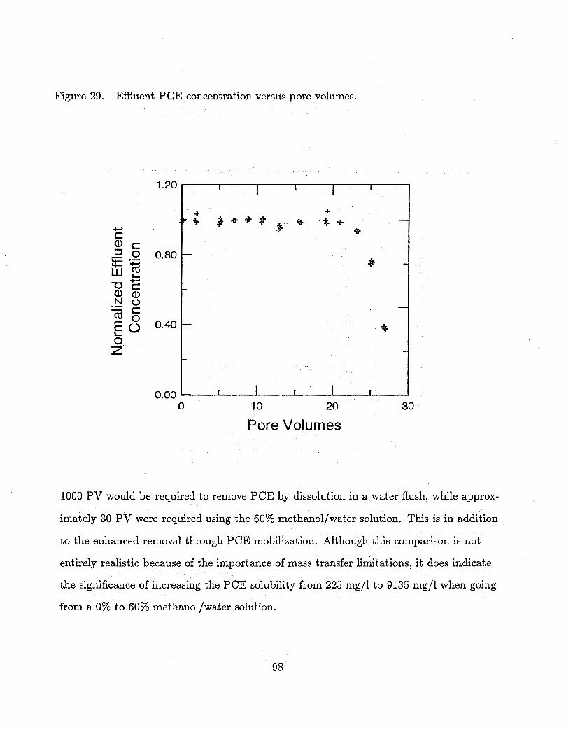
Figure 29. Effluent PCE concentration versus pore volumes.
0.00 I I I I I
0 10 20 30
Pore Volumes
1000 PV would be required to remove PCE by dissolution in a water flush, while approx-
imately 30 PV were required using the 60% methanol/water solution. This is in addition
to the enhanced removal through PCE mobilization. Although this comparison is not
entirely realistic because of the importance of mass transfer li&tations, it does indicate
the significance of increasing the PCE solubility from 225 mg/l to 9135 mg/l when going
from a 0% to 60% methanol/water solution.

2.3.8 Mass Transfer Rate Coefficient
To quantify the rate of mass transfer associated with the dissolution of PCE in the meth-
anol/water mixture, the importance of additional mass transfer mechanisms must be as-
sessed. As a methanol/water mixture moves into a region with residual PCE, the meth-
anol and water may partition into the PCE ganglia. According to the data obtained in
batch experiments for the methanol/water/PCE system, the equilibrium concentration
of methanol in PCE was less than 0.2% by volume for a 60% methanol/water mixture.
In addition, the partitioning of water into PCE was negligible. Thus, these additional
mass transfer processes can be neglected in the analysis of column experiments.
Following the procedure of Imho$ e t aE. [1994a], the PCE saturation and effluent PCE
concentrations can be used to compute the mass transfer rate coefficient for PCE disso-
lution, Kz, at various locations along the column:
where Kz is the mass transfer rate coefficient; x is the distance.from inlet; t is the time;
S, is the PCE saturation; Cs is the equilibrium PCE concentration in the aqueous phase;
99

C(0, t ) and C(L, t ) are PCE concentrations at the inlet and outlet of the porous medium,
respectively; p n is the NAPL phase density; 4 is the porosity; and U is the Darcy flux of
the aqueous phase.
Equations (20) and (21) were obtained by simplification of the advection-dispersion-
dissolution equation (Imhoget al., 1994a). As stated in equations (20) and (21), K1 is a
function of parameters measured experimentally: 4(x), C(0, t ) or C(Z, t ) , and aS,/at(z, t) .
The profile of PCE saturation versus time obtained by using x-ray attenuation measure-
ments for x ,= 7.25 cm is shown in Figure 30 for illustration. PCE saturation began to
decrease at approximately three hours after beginning the 60% methanol/water flush
and then decreased in an almost linear fashion until at 16 hours PCE saturation was
below the detection limit. Polynomials varying in degree from three to seven were fit
to the saturation versus time data at each column location, and the derivative of these
polynomials was used to estimate aS,/at(x,t). In Figure 30 the fitted polynomial was of
the seventh degree.
The mass transfer coefficient, Kl, can be calculated by using the PCE concentration
at either the column inlet (20) or outlet (21). Comparison of K l calculated by the two
equations permits an examination of the effect of any mass balance error on computed
K1: the s u m of the first two terms in the denominator of equations (20) and (21) are
calculated values of C(x,t), and differences in these calculated values represent mass bal-
ance errors (or errors in estimated C(x,t)) associated with x-ray measurement of PCE
saturations within the column.
Errors in computing KI arise from several sources: +(x), aS,/at(x,t), and C(z,t). 1mho.f
e t al. [1994a] performed an error analysis which indicated that for the majority of the
100

Figure 30. PCE saturation versus time for x = 7.25 cm.
W 0 CL
0.20
0.1 5
0.10
0.05
0.00
1 I 1 I 1 I 1
Polynomial Fit
+ Data
0 5 10 15 20
Time (hrs)
data the largest source of error in Kl arises from errors in computed C(x,t). For this
reason, an estimate for the error in Kl can be made from
IKI equation (20) - KZ equation(21) I Kt equation (20)
estimated percent error in Kl =
101

If the estimated percent error in K I is large, then the determination of C(x,t) is in er-
ror and has a significant effect on Kl. Only those values of Ki computed from (20) were
used for which the estimated percent error is less than 20%-
The programmed series of x-ray measurements during PCE dissolution were performed
only for the upper 12.5 cm of the column. Using equations (20) and (21), Ki could be
computed only for these column locations. In this case, C(0,t) is the inlet PCE con-
centration which was taken as zero, and C(L,t ) corresponds to the PCE concentration
12.5 cm below the column inlet. Although this concentration was not measured, it could
be inferred from the x-ray measurements: when x-ray measurements indicated that PCE
saturation was not changing at x = 12.5 em, C(12.5,t) C,. Mass transfer was not
occurring because of dissolution, which would happen only if the aqueous-phase PCE
concentration was at the solubility limit. Once PCE saturations began to decrease at
x = 12.5 cm, C(12.5,t) was unknown and equation (21) could not be used to estimate
Kl was computed using equations (20) and (21) for the locations x = 1.75 cm through
z = 3.25 cm and are shown as a function of changing Sn in Figure 31. Data are shown
for which the estimated error in K1 is less than 20%; sensitivity analyses indicated that
fitted models for Kl were insensitive to the value of the error norm at or below this value.
Kl were computed for other column locations, but equation (22) could not be used to
estimate the error for these data since C(12.5,t) was unknown for the times when ac-
tive mass transfer was occurring in these regions. Thus, the greatest confidence could be
placed in data at locations x = 1.75 em through x = 3.25 cm, and only these data were
used in regression analyses.
102

w e 31, Mass transfer sate coefficient versus changing PCE volumetric fraction for sampling locations x = 1.75, 2.25, 2.75, and 3.25 cm.
k-
80
40
- 0 0.00 0.01 0.02 0.03 0.04
e n
The data were put in dimensionless form and power-law models including Sh, Re, Sc,
and 6 , were fit to the data. The model used here was
103

This is the same model used earlier for flushing with heated water. In this experiment
the Darcy flux was kept constant and only 6, was varied: thus, R e changed minimally
during the experiment. Therefore, for the regression analyses, values of PI and
chosen based on the work of other investigators: a value of 0.75 was chosen for p1 and
0.5 for p 3 . 0.75 was chosen because of similar values successfully fitted in earlier investi-
were
gations (see discussion earlier for flushing with heated water). 0.5 was selected because
this was the recommended value from the experiments with heated water.
Nonlinear regression was used to fit the data to equation (23) with the selected values
for p1 and P 3 using SYSTAT [1988]. The best-fit parameters with 95% confidence inter-
vals are
Po = 0.41 f 0.27
pz = 0.57 f 0.16 (24)
The value of P 2 is smaller than values fitted by other investigators for transient dissolu-
tion: 0.87 was reported by Imho$ et al. [1994a], while Powers e t al. [1994] reported
values ranging from 0.75 to 0.96, depending on porous media characteristics. p 2 is clos-
est to the value of 0.60 reported by Milker et al. [1990], but those data were for steady-
state dissolution and not the transient dissolution of NAPL ganglia. The low value of pz is due to the influence of the two data points at the largest 6, shown in Figure 31; more
data for 6, 2 0.03 may yield a different exponent.
To evaluate P o , Sh is plotted versus 6, in Figure 32 for the model fitted here and for
those from other investigations using conditions in this work. The correlations of Imhofl
104

et al.
fered by a factor of two between their experiments and this study. The model shown
from ImRofl et a&.
bypassing associated with dissolution fingers occurred (.&mho$ et al.
[1994a] and Powers et al. E19941 were modified to include SC' *~ , since SC'*~ dif-
[1994a] is for conditions near the inlets to their columns before flow
1994b).
Figure 32. Comparison of predicted Sh from several correlations for NAPL dissolution with the best-fit model from the 60% methanol/water dissolution experiment.
~
10.00
Miller et al. (1 990 )
lmhoff et ai. (1 994a), model 4 with x ,/d = 7, modified to include Sco.'
Powers et al. (1994), modified to include SCO.~
60% methanoywater experiment
- - - - - - - -
- -
0.01 ' I I I I I I I 1 0.00 0.02 0.04 0.06 0.08
n e
105

The data from the 60% methanol/water experiment are approximately twice as small as
that predicted from the correlation of P o w e r s et al.
prediction from Imh et al.
Mdker e t al.
most similar to those employed by Powers e t al. [1994a], and
these correlations were expected to be in closest agreement with results from this work.
[1994], five times smaller than the
[1994a], and nine times smaller than the prediction from
[1990]. The procedures for creating the NAPL residual in this study axe
[1994] and Imho$ et al.
One explanation for the differences in mass transfer between the experiment reported
here and the experiments of Powers e t al.
ferences in the initial residual PCE. After PCE invasion the average PCE volumetric
content between x = 1.75 cm and x = 3.25 cm was 0.11, However, NAPL volumetric
contents before displacement were always greater than 0.25 in the experiments of P o w -
ers e t ab. [1994]. The smaller invasion NAPL saturations in
this study suggest that NAPL invaded fewer, smaller pores at the very top of the column
than in the other studies (Powers et al., 1994; Imho$ e t al., 1994). After NAPL dis-
placement with a water flood, a larger fraction of the trapped NAPL ganglia occupied
large pores than in other investigations. Thus for the same NAPL volumetric content,
NAPL dissolution in this study may have occurred from a smaller number of ganglia
[1994] and Imho$ et al. [1994a] may be dif-
[1994] and Imho$ e t al.
that were larger in size than in other investigations. Fewer, larger ganglia would have
a smaller total area for mass transfer and result in smaller dissolution rates for the same
NAPL volumetric content.
This explanation for the differences in observed mass transfer rates is plausible. The ef-
fect of methanol on IFT is not accounted for in the models for Kl and also may have in-
fluenced the dissolution rate. Further research is required to quantify the effect of NAPL
emplacement procedure and changes in IFT on NAPL dissolution. Even noting these
106

differences the data reported here are within a factor of five of predictions from correla-
tions developed by experimenters for similar porous media and somewhat similar NAPL
emplacement procedures and in one case within a factor of two.
2.4 Discussion
2.4.1 Physical and Chemical Properties
All of’the important physical and chemical properties of the PCE/methanol/water sys-
tem were measured or taken from reliable literature sources. The effects of methanol on
physical and chemical properties of the PCE/methanol/water system are summarized in
Table 18.
Table 18. Effects of methanol increase from 0% to 60% methanol fraction on properties.
Property
PCE solubility in aqueous phase MeOH solubility in nonaqueous phase Water content in nonaqueous phase Density (nonaqueous phase) Density (aqueous phase) Interfacial tension Viscosity (aqueous phase) Diffusivity (PCE in aqueous phase)
Change
+3960% 3159 mg/l
+22% -0.3% -9% -73% +72% -41%
Source
measured measured measured measured measured measured
Flick: [1991] predicted from
Wilke and Chang [1955]
107

Methanol was found not to partition significantly into the PCE unless methanol concen-
trations were large enough that the PCE became completely miscible with the aqueous
phase (methanol volumetric fractions 2 80%). Thus, an alcohol flush using methanol
in a PCEcontaminated aquifer is not expected to swell the PCE. However, methanol
did significantly afFect the viscosity of the aqueous phase, the interfacial tension between
the aqueous phase and PCE, the diffusivity of PCE, and the PCE solubility. There was
a small effect on the density difference between the nonaqueous and aqueous phases.
These latter effects will increase potential mobilization of trapped PCE droplets, alter
the mass transfer rate coefficient for dissolution, and reduce the number of pore volumes
required for remediation because of the increased PCE solubility. These effects were ob-
served in the enhanced remediation experiment described in the preceding section.
The UNIQUAC model was examined for predicting the phase partitioning behavior of
the PCE/methanol/water system. The relatively good predictions of this model suggest
that it may be useful for evaluating the partitioning behavior of other NAPL/water/
alcohol systems.
2.4.2 Mobilization
The addition of the 60% methanol/water mixture to the column resulted in the mobi-
lization of 28% of the PCE residual. The methanol increased the aqueous phase viscosity
from 0.89 cp to approximately 1.50 cp, decreased the nonaqueous-aqueous phase inter-
facial tension from 44.9 dynes/cm to 11.9 dynes/cm, and increased the density differ-
ence between the nonaqueous and aqueous phases from 0.615 g/ml to 0.701 g/ml. PCE
mobility is enhanced in this situation as interfacial forces trapping PCE droplets are re-
duced, and viscous and gravity forces enhanced.
108

As discussed earlier, investigators commonly examine two dimensionless groupings to as-
sess the relative importance of these forces: the Capillary number, Ca = va,ua/una, the
ratio of viscous to interfacial forces; and the Bond number, Bo = (pn - pa)gdg/4una, the
ratio of gravity to interfacial forces. In this experiment, the addition of the 60% meth-
anol/water mixture increased Ca from 1.7 x
0.0097 (based on dpl = d50 = 0.0277 cm). The increase in Ca is not the likely cause
of PCE mobilization, since experiments in glass bead media by Morrow e t al. [1988]
indicate that viscous forces mobilize residual oil only for Ca 2 1.0 x lo-*. However,
PCE mobilization due to small increases in Bo was observed by Morrow et al.
For similar increases in B o they observed decreases in oil saturation that, within exper-
imental error, were in agreement with the results from the 60% methanol/slash water
experiment.
to 6.3 x and Bo from 0.0026 to
[1988].
The significant PCE mobilization observed in the methanol/water experiment is likely
due to the effect of microlayering on the creation of high PCE residuals. As water im-
bibed it may have bypassed PCE in the coarser media immediately above fine layers,
trapping PCE islands consisting of many pores. Large pores and clusters of large pores
surrounded by smaller pores have been observed to retain all of their nonwetting phase
in imbibition experiments (Chatzis et al., 1984). This mechanism would result in higher
levels of PCE residual immediately above fine layers, which is consistent with the x-ray
measurements. Higher levels of PCE residual suggest larger PCE ganglia, which may be
more easily mobilized (Ng e t ai., 1978).
Further work is required to better quantify the effect of changes in Bo on buoyancy-
driven mobilization of NAPL ganglia. However, it is clear from this experiment that
flushing with a methanol/water mixture may enhance downward migration of NAPL
109

ganglia. Remediation of NAPL-contaminated sites with methanol/water mixtures must
account for this possibility.
2.4.3 Dissolution
The methanol/water mixture affected both the rate of PCE dissolution and the solu-
bility limit of PCE in the aqueous phase. The measured mass transfer rate coefficients
were within a factor of two of predictions from an existing correlation, suggesting that
the dimensionless groupings used in these models adequately account for the effect of the
methanol/water mixture on the physical and chemical properties affecting mass transfer.
Assuming that this is true, Kl can be predicted with equations (23) and (24) for rep-
resentative conditions and methanol/water fractions not used in this experiment. Pre-
dieted Kl are shown in Figure 33. For methanol volumetric fractions from 0% to 80% Kl
does not change by more than 25%.
The maximum potential enhancement of PCE dissolution due to a methanol/water mix-
ture is illustrated by plotting the maximum potential mass flux, KlC,, versus methanol/
water fraction. This is shown in Figure 34, where Ki was estimated from equations (23)
and (24), and C, taken from measured solubilities. The maximum potential mass flux
increases by one order of magnitude as the methanol/water fraction increases from 0%
to 60%. This dramatic improvement in the mass flux is due to the increase in aqueous
phase PCE solubility. This effect was demonstrated in the enhanced remediation exper-
iment, where the number of pore volumes required for cleanup was decreased from over
1000 to approximately 30 by the use of the 60% methanol/water mixture.
110

Figure 33. Predicted Ka for PCE ~ Q S representative conditions using equations (23) and (24).
1 1 1 I I I I I I
- - -
-
-
-
- I I I I I I I I I
80
70
60
50
40
U = 1.76 dday
e = 0.02 n
@ = 0.37
0.0 0.2 0.4 0.6 0.8 1 .o Methanol Fraction by Volume
(Aqueous Phase)
111

Figure 34. Maximum. potential mass flux of PCE for representative conditions using equations (23) and (24).
1000
100
10 0.0 0.2 0.4 0.6 0.8 1 .o
Methanol Fraction by Volume (Aqueous Phase)
112

References
Abrams, A. October 1975. The Influence of Fluid Viscosity, Interfacial Tension, and Flow Velocity on Residual Oil Saturation Left by Waterflood. Society of Petroleum Engineers Journal. :437447.
Abrams, D. S., and J. M. Prausnitz. 1975. Statistical Thermodynamics of Liquid Mix- tures: A New Expression for the Excess Gibbs Energy of Partly or Completely Mis- cible Systems. AIChE Journal. 21:116-128.
American Institute of Chemical Engineers. 1985. Data Compilation Tables of Properties of Pure Compounds. New York: AIChE.
American Society for Testing and Materials. 1991. Standard Test Method for Interfacial Tension of Oil Against Water by the Ring Method. Annual Book of ASTM Stan- dards, Designat on D 971-91, 15.04:300-302.
American Society for Testing and Materials. 1992. Standard Test Method for Water Us- ing Karl Fischer Reagent. Annual Book of ASTM Standards, Designation E203-92. 15.05~264-272.
Antonov, G. N. 1907. Tension at the Limit of Two Layers. J. Russ. Phys. Chem. SOC. 93:342.
Baibakov, N. K., and A. R. Garushev. 1989. Thermal Methods of Petroleum Production. New York: Elsevier.
Banerjee, S., S. H. Ydkowsky, and S. C. Valvani. 1980, Water Solubility and Octanol/ Water Partition Coefficients of Organics. Limitations of the Solubility-Partition Co- efficient Correlation. Environmental Science & Technology. 14( 10):1227-1229.
1989. Methods for Dissolving Hydrophobic Compounds in Water: Interactions with Dissolved Organic Matter. In Aquatic Humic Substances. American Chemical Soci- ety.
I Barrie Webster, G. R., M. R. Servos, G. G. Choudhry, L. Sarna, and D. C. G. Muir.
Barton, A. F. M. 1975. Chemical Reviews. 75:731-753.
Basel, M. D., and K. S. Udell. 1989. Two-Dimensional Study of Steam Injection into Porous Media. Multiphase Transport in Porous Media. ASME HTD-127.
Basel, M. D., and K. S. Udell. 1991. Effect of Heterogeneities on the Shape of Condensa- tion Fronts in Porous Media. Heat !l!ransfer in Geophysical Media. ASME HTD-172.
Bear, J. 1979. In Hydraulics of Groundwater. New York: McGraw-Hill, p. 567.
113

Bellocq, A. M., D. Bourbon, and B. Lemanceau. 1981. Thermodynamic, Interfacial and Structure Properties of Alcohol-Brine-Hydrocarbon Systems. J. Disp. Sci. Tech , 2:227.
Bharath, A,, C. Mallard, D. Om, G. Qzburn, and A. Smith. 1984. Problems in Deter- mining the Water Solubility of Compounds. Bul l e t in of Env i ronmen ta l Con tamina- t i o n and Toxicology. 33:133-137.
Billington, J. W., G. Huang, F. Szeto, W. Y. Shiu, and D. Mackay. 1987. Preparation of Aqueous Solutions of Sparingly Soluble Organic Substances: I. Single Component Systems. Env i ronmen ta l Toxicology & Chemis t ry . 7:117-124.
Boberg, T. C. 1988. T h e r m a l Methods of Oil Recovery. New York: John Wiley.
Boyd, G. R. 1991. Factors Influencing Nonaqueous Phase Liquid Removal from Ground Water by Alcohol Flooding. Ph.D. Dissertation, Clemson University, Clemson, SC.
Brandes, D. 1992. Effect of Phase Behavior on Residual Dense Nonaqueous Phase Liq- uid Displacement from Porous Media by Alcohol Flooding, M.S. Thesis, Clemson University, Clemson, SC.
Brandes, D., and K. J. Farley. November-December,l993. Importance of Phase Behav- ior on the Removal of Residual DNAPLs from Porous Media by Alcohol Flooding. Journa l of W a t e r Env i ronmen t Research. 65(7):869-878. .
Buerger, J., P. Sourieu, and M. Combarnaus. 1985. T h e r m a l Methods of Oil Recovery. Paris: Gulf Publishing.
Chatzis, I., M. S. Kuntamukkula, and N. R. Morrow. 1984. Blob-Size Distribution as a Function of Capillary Number in Sandstones. Dallas, TX: Society of Petroleum Engineering of AIME.
Coca, J., and R. Diaz. 1980. Extraction of Furfural from Aqueous Solutions with Chlori- nated Hydrocarbons. Journal of Chemical Engineering Data. 25( 1):80-83.
Cullinan, H. T. Jr., and M. R. Cusick. 1967. A Predictive Theory for Diffusion in Mixed Solvents. AIChE Journal. 13:1171-1174.
Davis, E. L., and B. K. Lien. May 1993. Laboratory Study on the Use of Hot Water to Recover Light Oily Wastes from Sands. Ada, OK: US EPA Robert S. Kerr Environ- mental Research Laboratory.
De Visser, C. G., G. Perron, and J. E. Desnoyers. 1977. The Heat Capacities and Expan- cibilities of Tert-Butyl Alcohol-Water Mixtures from 6 to 65 C. Canad ian Journa l of Ch emis tr y . 55: 8 5 6-862.
1
Demond, A. H. 1988. Capillarity in Two-Phase Liquid Flow of Organic Contaminants in Groundwater, Ph.D. Dissertation, Stanford University, Stanford, C A.
114

DeVoe, H., M. M. Miller, and S. P. Wasik. 1981. Generator Columns and High Pressure Liquid Chromotography for Determining Aqueous Solubilities and Octanol Water Partition Coefficients. Journal of Research of the National Bureau of Standards. 86( 4):361-366.
Donahue, J. D., and F. E. Bartell. 1952. The Boundary Tension at Water-Organic Liq- uid Interfaces. J. Phys. Chem. 56:480-484.
Donohue, D. A. T. 1963. A Mathematical Model to Simulate the Recovery of Water and Oil from Porous Media by the Injection of Solvents, Ph.D. Dissertation, The Penn- sylvania State University, University Park, PA.
DuPont de Nemours and Company, I. 1966. Solvent Properties Comparison Chart.
Edmondson, T. A. May 1965. Effect of Temperature on Waterflooding. Journal of Cana- dian Petroleum Technology. :236-242.
Ethyl Corp. 1958. Chlorinated Solvents. Report ICD-1006(58).
Falta, R. W., K. Pruess, I. Javandel, and P. A. Witherspoon. February 1992a. Numerical Modeling of Steam Injection for the Removal of Nonaqueous Phase Liquids from the Subsurface, 1. Numerical Formulation. Water Resources Research. 28(2):433449.
Falta, R. W., K. Pruess, I. Javandel, and P. A. Witherspoon. February 1992b. Numerical Modeling of Steam Injection for the Removal of Nonaqueous Phase Liquids from the Subsurface, 2. Code Validation and Application. Water Resources Research.
28(2):451-465. J:
Flick, E. W. ed. 1991. In Industrial Solvents Handbook.. 4th Edition. Park Ridge, NJ: Noyes Data Corp. 930 p.
Fredenslund, A,, R. L. Jones, and J. M. Prausnitz. 1975. Group-Contribution Estimation of Activity Coefficients in Nonideal Liquid Mixtures. American Institute of Chemical Engineers. 21 (6) : 1086-1 099.
Fu, J., B. Li, and 2. Wang. 1986. Estimation of Fluid-Fluid Interfacial Tensions of Multi- Component Mixtures. Chemical Engineering Science. 41:2673-2679.
Gatlin, C., and R. L. Slobod. 1960. The Alcohol Slug Process for Increasing Oil Recov- ery. AIME. 219:46-53.
Geller, J. T. 1990. Dissolution of Non-Aqueous Phase Organic Liquids in Porous Media, Ph.D. Dissertation, University of California-Berkeley, Berkeley, CA.
Girifalco, L. A., and R. J. Good. 1957. A Theory for the Estimation of Surface and In- terfacial Energies, 1: Derivation and Application. Journal of Physical Chemistry. 61:904.
Gladis, G. P. 1960. Chemical Engineering Progress. 56( 10):43-51.
115

t
Gupte, P. A., and R. P. Danner. 1987. Prediction of Liquid-Liquid Equilibria with UNI- FAC A Critical Evaluation. Indus t r ia l and Engineering Chemis t ry . 26:2036-2042.
Hayduk, W., and H. Laudie. 1974. Prediction of Diffusion Coefficients for Nonelectrolytes in Dilute Aqueous Solutions. A m e r i c a n Ins t i t u t e of Chemical Engineers. 20(3):611- 615.
Holm, L. W., and A. K. Csaszar. 1962. Oil Recovery by Solvents Mutually Soluble in Oil and Water. Society of P e t r o l e u m Engineers Journal. 2:129-144.
Holmes, J. T., D. R. Olander, and C. R. Wilke. 1962. Diffusion in Mixed Solvents. AIChE Journal . 8:646-649.
Horvath, A. L. 1982. Halogenated Hydrocarbons Solubili ty-Miscibil i ty w i th W a t e r . New York: Marcel Dekker.
Hunt, J. R., N. Sitai, and K. S. Udell. 1988a. Nonaqueous Phase Liquid Transport and Cleanup 2. Experimental Studies. W a t e r Resources Research. 24(8):1247-1258.
Hunt, J. R., N. Sitar, and K. S. Udell. 198813. Nonaqueous Phase Liquid Transport and Cleanup 1. Analysis of Mechanisms. W a t e r Resources Research. 24(8):1247-1258,
Imhoff, P. T., P. R. Jaff6, and G. F. Pinder. 1994a. An Experimental Study of Complete Dissolution of a Nonaqueous Phase Liquid in Saturated Porous Media. W a t e r R e - sources Research. 30(2):307-320.
Imhoff, P. T., C. T. Miller, and G. P. Thyrum. 1994b. Dissolution Fingering During the Solubilization of Nonaqueous Phase Liquids in Saturated Porous Media, submit ted W a t e r Resources Research.
Kett, T. K., and D. K. Anderson. 1969. Multicomponent Diffusion in Nonassociating, Nonelectrolytes Solutions. Journa l of Physical Chemis t ry . 75:1262-1267.
Knickerbocker, B. M., C. V. Pesheck, L. E. Scriven, and H. T. Davis. 1979. Phase Be- havior of Alcohol-Hydrocarbon-Brine Mixtures. Journa l of Physical Chemistry . 83( 15) ~1984-1990.
Lake, L. W. 1983. Enhanced Oil Recovery f o r Independen t Producers. Dallas, TX: South- ern Methodist University.
Lam, A. C., R. S. Schechter, and W. D. Wade. Oct 1983. Mobilization of Residual Oil under Equilibrium and Nonequilibrium Conditions. SPEJ. :781-790.
Larson, R. G., H. T. Davis, and L. E. Scriven. 1982. Elementary Mechanisms of Oil Re- covery by Chemical Methods. J o u r n a l of Pet ro leum Technology, 34:243-258.
Leffler, J., and H. T. Cullinana Jr. 1970. Variation of Liquid Diffusion Coefficients with Composition, Dilute Ternary Systems. Industr ial and Engineering Chemis t ry Funda- m e n t als . 9: 88-93.
116

Lide, D. R. ed. 1990. CRC Handbook: of Chemistry and Physics. Boston: CRC Press.
Lo, H. Y., and N. Mungan. Effect of Temperature on Water-Oil Relative Permeabilities in Oil-Wet and Water-Wet Systems. In SPE of AIME, 48th Annual Fall Meeting.
Lyman, W. J., W. F. Reehl, and D. H. Rosenblatt. 1982. Handbook of Chemical Property Estimation Methods: Environmental Behavior of Organic Compounds. New York: McGraw-Hill.
May, W. E., S. P. Wasik, and D. K. Freeman. 1978. Determination of the Aqueous Sol- ubility of Polynuclear Aromatic Hydrocarbons by a Coupled Column Liquid Chro- matographic Technique. Analytical Chemistry. 50( 1) :175-179.
McBride, J. F., and C. T. Miller. 1994. Measurement of Phase Fkactions in Porous Me- dia by Using X Rays 2. Applications. submitted Water Resources Research. .
McCaffery, F. G. 1972. Measurement of Interfacial Tensions and Contact Angles at High Temperature and Pressure. Journal of Canadian Petroleum Technology. :26-32.
McGovern, E. W. 1943. Chlorohydrocarbon Solvents. Ind. Eng. Chem. 35:1230-1239.
Melrose, J . C., and C. F. Branden. 1974. Role of Capillary Forces in Determining Mi- croscopic Displacement Efficiency for Oil Recovery. Journal of Canadian Petroleum Technology. 13(1):13.
Miller, C. T., M. M. Poirier-McNeill, and A. S. Mayer. 1990. Dissolution of Trapped Nonaqueous Phase Liquids: Mass Transfer Characteristics. Water Resources Re- search. 26( 11):2783-2796.
Millington, R. J., and J. P. Quirk. 1961. Permeability of Porous Solids. Transactions of the Faraday Society. 57:1200-1207.
Moiseeva, L. M., G. G. Stepanova, and A. N. Pukhonto. 1977. Solubility of Tetrachloro- ethylene in Aqueous Electrolyte Solutions. Khim. Prom. 6:435-437.
Montgomery, J. H. 1991. Tetrachloroethylene. In Groundwater Chemicals Field Guide.
Morrow, N. R., I. Chatzis, and J. J. Taber. August 1988. Entrapment and Mobilization
MI: Lewis Publishers.
of Residual Oil in Bead Packs. SPE Reservoir Engineering. :927-934.
Ng, K. M., H. T. Davis, and L. E. Scriven. 1978. Visualization of Blob Mechanics in Flow Through Porous Media. Chemical Engineering Science. 33:1009-1017.
Noda, K., M. Ohashipnd K. Ishida. 1982. Viscosities and Densities at 298.15 K for Mix- tures of MEthanol, Acetone and Water. Journal of Chemical Engineering Data. 27:326-328.
117

Parker, J. C., A. K.,Katyal, J. J. Kaluarachchi, R. J. Lenhard, T. J. Johnson, K. Jayara- man, K. Unlu, and J. L. Zhu. 1991. Modeling Multiphase Organic Chemical Trans- port in Soils and Ground Water, Report EPA/600/2-91/042, U.S. Environmental Protection Agency, Washington, D. C.
Patwardhan, S. 1992. Effect of Alcohol Concentration on Efficiency of Alcohol Flood in Groundwater Remediation, M.S. Thesis, Clemson University, Clemson, SC.
Pausell, W. G. 1953. The Effect of Mutually Miscible Intermediate Phase on Immisci- ble Fluid Displacement in a Porous Medium, M.S. Thesis, University of Oklahoma, Norman, OK.
Pinal, R., P. S. Rao, L. S. Lee, and P. V. Cline. 1990. Cosolvency of Partially Miscible Organic Solvents on the Solubility of Hydrophobic Organic Chemicals. E n v i r o n m e n - t a l Science & Technology. 24(5):639-647.
Powers, S. E., L. M. Abriola, and W. J. Weber Jr. 1992. An Experimental Investigation of Nonaqueous Phase Liquid Dissolution in Saturated Subsurface Systems - Steady State Mass Transfer Rates. W a t e r Resources Research. 28(10):2691-2705.
Powers, S. E., L. M. Abriola, and W. J. Weber Jr. 1994. An Experimental Investigation of Nonaqueous Phase Liquid Dissolution in Saturated Subsurface Systems - Tran- sient Mass Transfer Rates. W a t e r Resources Research. 30(2):321-332.
Prausnitz, J., T. Anderson, E. Grens, C. Eckert, R. Hsieh, and J. O'Connell. 1980. Com-3 p u t e r Calculations f o r Mult icomponent Vapor-Liquid and Liquid-Liquid Equilibria. Englewood Cliffs, NJ: Prentice-Hall.
Quittier, L., and B. Corre. February 1988. Hot-Water Steamflood Laboratory Experi- ments under Reservoir Conditions. Society of P e t r o l e u m Engineers Reservoir Eng i - nee ring. ; 149-1 5 7.
Reed, R. L., and R. N. Healy. 1977. Improved Oil Recovery by Sur fac tan t and P o l y m e r
Reid, R. C., J. M. Prausnitz, and B. E. Poling. 1987. T h e Propert ies of Gases and L iq -
Flooding. NY: Academic Press.
uids. New York: McGraw-Hill.
Row-Desgrandes, G. A,, A. H. Roux, J. P. Groilier, and A. Vialard. 1981. Apparent Molar Heat Capacities of Microemulsion. Journa l of Colloid a n d Interface Science. 84:536.
Rubino, J. T., J. Blanchard, and S. H. Yalkowsky. 1984. J. Paren t . Sei . Technol. 38:215- 221.
Rubino, J. T., and S. H. Yalkowsky. 1985. J. Parent . Sci . Technol. 39:106-111.
Sayar, A. A. 1991. Liquid-Liquid Equilibria of Some Water + 2-Propanol + Solvent Ternaries. J o u r n a l of Chemical Engineering Data. 36( 1):61-65.
118

Sconce, J. S. ed. 1962. Chlorine: Its Manufacture, Properties and Uses. NY: Reinhold Publishing Corp.
Schwille, F. 1988. Dense Chlorinated Solvents in Porous and Fractured Media. Chelsea, MI: Lewis Publishers, Inc.
Stephenson, R. M, 1992. Mutual Solubilities: Water-Ketones, Water-Ethers, and Water- Gasoline- Alcohols. Jo urn aE of Ch e mi cal Engineering Data. 3 7: 80-95.
Steward, L. D. Jr., and K. S. Ude11..1989. Multiphase Transport in Porous Media.
Stoval, S. L. August 13, 1934. Recovery of Oil from Depleted Sands by Means of Dry Steam. Oil Weekly. 73:17-24.
SYSTAT Incorporated; 1988. SYSTAT, The System for Statistics. Evanston, IL.
Sufi, A. H., H. J. Ramey Jr., and W. E. Brigham. 1982. Temperature’s Effect on Rela- tive Permeabilities of Oil-Water Systems. In SPE of AIME, 57th Annual Fall Tech- nical Conference and Exhibition.
c
Taber, J. J. 1969. Dynamic and Static Forces Required to Remove a Discontinuous Oil Phase from Porous Media Containing Both Oil and Qater. SPE Journal. 2:3-12.
Taber, J. J., I. S. K. Kamath, and R. R. Reed. 1961. Mechanism of Alcohol Displace- ment of Oil from Porous Media. Society of Petroleum Engineers Journal. 1:195-212.
Tyn, M. T., and W. F. Calus. 1975. Temperature and Concentration Dependence of Mu- tual Diffusion Coefficients of Some Binary Liquid Systems. Journal of Chemical and Engineering Data. 20(310-316).
Udell, K. S. 1992. Technologies of Contaminant Removal: Thermally Enhanced Removal of the Oily Phase. In Subsurface Restoration Conference. pp. 51-53.
United States Environmental Protection Agency. November, 1992. The Superfund Inno- vative Technology Evaluation Program. Cincinnati, OH: Risk Reduction Engineer- ing Laboratory.
U.S. Coast Guard. 1978. CHRIS Hazardous Chemical Data. Washington, D.C.: U.S. Government Printing Office.
Veith, G. D., and V. M. Comstock. 1975. Apparatus for Continuously Saturating Water with Hydrophobic Organic Chemicals. J. Fish. Res. Board Can. 32:1849-1851.
Volek, C. W., and J. A. Pryor. 1972. Steam Distillation Drive-Brea Field, California. Journal of Petroleum Technology. 242399-906.
Wachman, C. 1963. A Mathematical Theory for the Displacement of Oil and Water by Alcohol. In Presented a t the 24th Technical Conference on Petroleum Production at
119

T h e Pennsy lvan ia S t a t e Universi ty , Minera l Industr ies E z p e r i m e n t S t a t i o n Circular No. 66. pp. 27.
Walace, S. M. 1985. P h a s e Equilibria in Chemical Engineering. Stoneham, MA: Butter- worth.
Wasik, S. P., M. M. Miller, Y. B. Tewari, W. E. May, W. J. Sonnefeld, H. DeVoe, and W. H. Zoller. 1983. Determination of the Vapor Pressure, Aqueous Solubility, and Octanol/Water Partition Coefficient of Hydrophobic Substances by Coupled Gener- ator Column/Liquid Chromotographic Methods. Residue Reviews. 85:2942.
Weast, R. C. ed. 1985. Handbook of C h e m i s t r y and Physics. 65th Edition. Cleveland, OH: CRC Press.
Wilke, C. R., and P. Chang. 1955. Correlation of Diffusion Coefficients in Dilute Solu- tions. A m e r i c a n Ins t i t u t e of Chemcia l Engineering Journal. 1:264-270.
Williams, N. A,, and G. L. Amidon. 1984. Excess Free Energy Approach to the Estima- tion of Solubility in Mixed Solvent Systems - I. Theory. Journa l of PharmaceuticaZ Sciences. 73( 1):9-13.
Willman, B. T., V. V. Valeroy, G. W. Runberg, Cornelius A. L., and L. W. Powers. July 1961. Laboratory Studies of Oil Recovery by Steam Injection. J o u r n a l of Pet ro leum Technology. :681-690.
Wilson, J. L., S. H. Conrad, W. R. Mason, W. Peplinksi, and E. Hagan. 1989. Labora- tory Investigation of Residual Organics from Spills, Leaks, and the Disposal of Haz- ardous Wastes in Groundwater. Ada, OK: Robert S. Kerr Laboratory, U S . Environ- mental Protection Agency.
Wright, W. H., and J. M. Schaffer. 1932. Anthelmintic Properties. Am, J . Hyg. 16(2):325- 428.
Yalkowsky, S. H. 1986. Project Completion Report, CR 812581-01. Ada, OK: U. S. Envi- ronmental Protection Agency.
Yuan, 2. G., and K. S. Udell. March 1993. Steam Distillation of a Single Component Hy- drocarbon Liquid in Porous Media. In t e rna t iona l Journa l of Heat and M a s s Trans- f e T. 36 (4) : 88 7-897.
Zenon Environmental Inc. November 1986. A Study of Enhanced Dissolution for the In Situ Remediation of Dense Non-Aqueous Phase Liquid (DNAPL) Chemicals in the Subsurface. Environmental Canada.
120