an existence result for singular liouville equations on compact ... …daruiz/investigacion/slides...
TRANSCRIPT

Introduction to the problem The result Case 1 Case 2
An existence result for singular Liouvilleequations on compact surfaces.
David Ruiz
Departamento de Análisis Matemático (Universidad de Granada, Spain)
joint work with Andrea Malchiodi (SISSA).

Introduction to the problem The result Case 1 Case 2
The problem
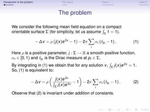
We consider the following mean field equation on a compactorientable surface Σ (for simplicity, let us assume
´Σ
1 = 1).
−∆v = ρ(j(x)e 2v − 1
)− 2π
∑i
αi (δpi − 1) . (1)
Here ρ is a positive parameter, j : Σ→ R a smooth positive function,αi ∈ [0,1) and δpi is the Dirac measure at pi ∈ Σ.
By integrating in (1) we obtain that for any solution v ,´
Σj(x)e 2v = 1.
So, (1) is equivalent to:
−∆v = ρ
(j(x)e 2v´Σ
j(x)e 2v − 1)− 2π
∑i
αi (δpi − 1) . (2)
Observe that (2) is invariant under addition of constants.
Introduction to the problem The result Case 1 Case 2
The problem
We consider the following mean field equation on a compactorientable surface Σ (for simplicity, let us assume
´Σ
1 = 1).
−∆v = ρ(j(x)e 2v − 1
)− 2π
∑i
αi (δpi − 1) . (1)
Here ρ is a positive parameter, j : Σ→ R a smooth positive function,αi ∈ [0,1) and δpi is the Dirac measure at pi ∈ Σ.
By integrating in (1) we obtain that for any solution v ,´
Σj(x)e 2v = 1.
So, (1) is equivalent to:
−∆v = ρ
(j(x)e 2v´Σ
j(x)e 2v − 1)− 2π
∑i
αi (δpi − 1) . (2)
Observe that (2) is invariant under addition of constants.

Introduction to the problem The result Case 1 Case 2
Motivation from physicsThis equation arises from physical models such as the abelianChern-Simons-Higgs theory and the Electroweak theory. In thisframework, the points pi represent vortexes.
J. Hong, Y. Kim, P. Y. Pac, Phys. Rev. Lett. 1990.
R. Jackiw and E. J. Weinberg, Phys. Rev. Lett. 1990.
C. H. Lai (ed.), Selected Papers on Gauge Theory of Weak andElectromagnetic Interactions, World Scientific, Singapore, 1981.
G. Dunne, Self-dual Chern-Simons Theories, Lecture Notes inPhysics, Springer-Verlag 1995.
G. Tarantello, Self-Dual Gauge Field Vortices: An AnalyticalApproach, PNLDE 72, Birkhäuser Boston, 2007.
Y. Yang, Solitons in Field Theory and Nonlinear Analysis,Springer Monographs in Mathematics, 2001.

Introduction to the problem The result Case 1 Case 2
Motivation from conformal geometry
This problem is also related to the Kazdan-Warner problem when allαi = 0. The case αi 6= 0 refers to metrics with constant curvature butwhere pi is a conical point of Σ.
S.Y.A. Chang and P. C. Yang, Acta Math. 1987.
C. C. Chen and C.S. Lin, CPAM 2003.
J. Kazdan and F. Warner, Ann. of Math. 1974.
A. Malchiodi, review, DCDS to appear (available in his site).
G. Tarantello, review, DCDS 2010.
T. Aubin, Nonlinear Analysis on Manifolds. Monge-AmpèreEquations, Springer-Verlag, 1982.

Introduction to the problem The result Case 1 Case 2
A change of variablesLet wi be a solution of the problem:
−∆w = δpi − 1. (3)
Clearly, wi (x) ∼ −12π log |x − pi | for x close to pi . By making the
change of variables u = v + 2π∑
i αiwi , we pass to the problem:
−∆u = ρ
(h(x)e 2u´Σ
h(x)e 2u − 1). (4)
Here h(x) = j(x)e−4π∑
i αi wi . Observe that, close to pi ,h(x) ∼ |x − pi |2αi .
Equation (4) is the Euler-Lagrange equation for the functionalIρ : H1(Σ)→ R,
Iρ(u) =
ˆΣ
|∇u|2 + ρ(
2ˆ
Σ
u − logˆ
Σ
h(x)e2u). (5)

Introduction to the problem The result Case 1 Case 2
The energy functional
Iρ(u) =
ˆΣ
|∇u|2 + ρ(
2ˆ
Σ
u − logˆ
Σ
h(x)e2u). (6)
Recall the Moser-Trudinger inequality
logˆ
Σ
e2u ≤ 14π
ˆΣ
|∇u|2 + 2ˆ
Σ
u + C; u ∈ H1(Σ), (7)
J. Moser, A sharp form of an inequality by N.Trudinger, Indiana U.M. J. 1971.
L. Fontana, Sharp borderline Sobolev inequalities on compactRiemannian manifolds, Comm. Math. Helvetici 1993.
Then Iρ is bounded from below if ρ ≤ 4π. If ρ < 4π, the functional isalso coercive and there exists a minimum.
Moreover, if ρ > 4π, Iρ(ϕλ)→ −∞ as λ→ +∞, where:
ϕλ(x) = log(
λ
1 + λ2dist(x , x0)2
), x0 6= pi .

Introduction to the problem The result Case 1 Case 2
The previous choice is not casual: indeed, the functions defined in R2:
U(x) = log(
λ
1 + λ2|x − x0|2
), λ > 0, x0 ∈ R2,
are the unique entire solutions of the problem:
−∆U(x) = 4e2U(x), x ∈ R2
with e2u ∈ L1(R2).
W. Chen and C. Li, Classification of Solutions of Some NonlinearElliptic Equations, Duke Math. J. 1991.
Here we will consider ρ > 4π and look for critical points of Iρ by usingmin-max techniques.

Introduction to the problem The result Case 1 Case 2
The result
TheoremTake 0 = α0 < α1 ≤ α2 ≤ . . . αk . Assume ρ ∈ (4π,8π), ρ 6= 4π(1 + αi )for any i.Assume also that either Σ is not homeomorphic to a sphere orρ /∈ (4π(1 + αk−1),4π(1 + αk )).Then problem (1) has a solution.
The cases ρ = 4πk , ρ = 4π(k + αi ) are intrinsically more delicate.Existence results are given, for αi = 0, in:
S.Y.A. Chang and P. C. Yang, Prescribing Gaussian curvature onS2, Acta Math. 1987.
C. C. Chen and C. S. Lin, Topological degree for a mean fieldequation on Riemann surfaces, CPAM 2003.

Introduction to the problem The result Case 1 Case 2
For αi 6= 0 there seems to be some advance too:
C.-S. Lin, preprint.
The second condition may look technical. However, there holds:
TheoremAssume that k = 1, Σ = S2, ρ ∈ (4π,4π(1 + α)). If j(x) = 1, then (1)does not admit any solution.
D. Bartolucci, C.S. Lin and G. Tarantello, DCDS 2010.

Introduction to the problem The result Case 1 Case 2
The proof
Our approach is variational, and is based on the study of the topologyof the sublevels:
I−Mρ = u ∈ H1 : Iρ(u) ≤ −M,
for M large enough.
W. Ding, J. Jost, J. Li and G. Wang, Existence results for meanfield equations, AIHP 1999.
Z. Djadli, Existence result for the mean field problem on Riemannsurfaces of all genuses, Comm. Contemp. Math. 2008.
Z. Djadli and A. Malchiodi, Existence of conformal metrics withconstant Q-curvature, Ann. of Math. 2008.

Introduction to the problem The result Case 1 Case 2
Case 1: ρ ∈ (4π(1 + αk),8π).
Proposition
Assume h : Σ→ R with 0 ≤ h(x) ≤ C0. Let Ω1,Ω2 be two subsets ofΣ with dist(Ω1,Ω2) ≥ δ0 > 0, and fix γ0 > 0. Then, for any ε > 0 thereexists a constant C = C(C0, ε, δ0, γ0) such that
logˆ
Σ
h(x)e2u ≤ C +1
8π − ε
ˆΣ
|∇u|2 + 2ˆ
Σ
u.
for all functions u ∈ H1(Σ) satisfyingˆ
Ωj
h(x)e2u
ˆΣ
h(x)e2u≥ γ0, j = 1,2. (8)
W. Chen and C. Li, Prescribing Gaussian curvatures on surfaceswith conical singularities, J. Geom. Anal. 1991.

Introduction to the problem The result Case 1 Case 2
As a consequence we have that for any un ∈ H1 such thatIρ(un)→ −∞,
heunˆheun
δx
for some x ∈ Σ. This provides us with a continuous map:
Ψ : I−Mρ → Σ,
for M large enough.

Introduction to the problem The result Case 1 Case 2
Moreover, for λ > 0 large we define Φλ : Σ→ I−Mρ as:
Φλ[x0](x) = log[
λ
1 + λ2|x − x0|2(1+αk )
]for x in a neighborhood of x0.Again, those functions correspond to the unique entire solutions ofthe problem
−∆u = 4(1 + αk )2|x − x0|2αk e2u.
J. Prajapat and G. Tarantello, On a class of elliptic problems inR2: Symmetry and Uniqueness results, PRSE 2001.
In order to compute that indeed Iρ(Φλ[x0]) < −M for any x0 ∈ Σ weuse strongly that ρ > 4π(1 + αk ).

Introduction to the problem The result Case 1 Case 2
Topological properties of sublevels
We can compute the composition:
ΣΦλ−→ I−M
ρΨ−→ Σ.
It is possible to show that Ψ Φλ → Id as λ→ +∞. So, thecomposition is Ψ Φλ is homotopycally equivalent to the identity.
In other words, I−Mρ dominates Σ. In such case, it is known that
cat LS
(Φλ(Σ), I−M
ρ
)≥ cat LS
(Σ).
In particular, Φλ(Σ) is not contractible in I−Mρ for any λ large enough.
O. Cornea, G. Lupton, J. Oprea and D. Tanré, Lusternik-Schnirelmann category, Math. Surveys and Monographs vol103, AMS, 2003.

Introduction to the problem The result Case 1 Case 2
The min-max argument
Choose M ′ > M > 0 and λ > 0 such that Φλ(Σ) is not contractible inI−Mρ and Φλ(Σ) ⊂ I−M′
ρ .
Take C = tu : t ∈ [0,1], u ∈ Φλ(Σ). Clearly, Φλ(Σ) = ∂C iscontractible in C. Define:
Γ = h : H1(Σ)→ H1(Σ) homeomorphism : h|∂C = Id,
c = infγ∈Γmaxu∈C Iρ γ(u).
Observe that for any γ ∈ Γ, ∂C is contractible in γ(C).
By the previous topological argument, c ≥ −M > −M ′ ≥ Iρ|∂C .Therefore, there exists a (PS) sequence at level c.
Unfortunately, we do not know whether Iρ satisfies the (PS) conditionor not!

Introduction to the problem The result Case 1 Case 2
Existence for almost all values of ρ
By using the so-called "monotonicity trick", we obtain that for almostall values of ρ ∈ (4π(1 + αk ),8π), there exists a bounded (PS)sequence.
L. Jeanjean, On the existence of bounded Palais-Smalesequences and applications..., PRSE 1999.
L. Jeanjean and J. F. Toland, Bounded Palais-Smalemountain-pass sequences, CRAS 1998.
M. Struwe, On the evolution of harmonic mappings ofRiemannian surfaces, Comment. Math. Helv. 1985.
Once the sequence is bounded, we can pass to a weak limit, and thishappens to be a strong limit and a solution of our problem.

Introduction to the problem The result Case 1 Case 2
Compactness of solutions
The following result holds:
TheoremLet un solve (4) with ρ = ρn → ρ0 and assume that ρ0 6= 4kπ,ρ0 6= 4π(k + α) for any k ∈ N. Suppose that
´Ω
eui ≤ C1 for somefixed C1 > 0. Then un is uniformly bounded from above on Σ;
D. Bartolucci and G. Tarantello, Liouville type equations withsingular data and their application ...,Comm. Math. Phys. 2002.
Y. Y. Li, Harnack type inequality: The method of moving planes,Comm. Math. Phys. 1999.
From that we conclude that un converges to a certain u ∈ H1, andthat u is a solution of (4) with ρ = ρ0.

Introduction to the problem The result Case 1 Case 2
Case 2: ρ ∈ (4π(1 + αi),4π(1 + αi+1))
In this case it seemed impossible to us to define a map Φλ : Σ→ I−Mρ
as before. The problem appears when defining Φλ[pj ], j > i .A result that may explain why is the following:
TheoremLet B be the unit ball of R2. Then, for any u ∈ H1(B) radial, thereholds:
logˆ
B|x |2αe2u ≤ 1
4(1 + α)π
ˆB|∇u|2 + 2
B
u + C.
J. Dolbeault, M. J. Esteban and G. Tarantello, A weightedMoser-Trudinger inequality and its relation to ..., Ann. Sc. Norm.Sup. Pisa Cl. Sci 2008.
That makes one think that now sublevels will not contain functionsconcentrated around some pi .

Introduction to the problem The result Case 1 Case 2
TheoremFix ρ ∈ (4π,8π). There exists M > 0 and a map β : I−M
ρ → Σ suchthat for any ε > 0
logˆ
Σ
|x − p|2αe2u ≤ 14π(1 + α)− ε
ˆΣ
|∇u|2 + 2ˆ
Σ
u + Cε,
for any u ∈ I−Mρ with β(u) = p.
Actually the map β applies to f = heu´heu . Let us define:
A = f ∈ L1(Σ), f (x) > 0 a.e.,ˆ
Σ
f = 1,
σ : Σ×A → (0,+∞),
where σ = σ(x , f ) is chosen such that (for some C > 0 large):ˆ
Bx (σ)
f =
ˆBx (Cσ)c
f .

Introduction to the problem The result Case 1 Case 2
A barycenter mapLet us define T : Σ×A → (0,+∞),
T (x , f ) =
ˆBx (σ(x,f ))
f .
Both σ and T are continuous.
There exists τ = τ(C) > 0 such that
maxx∈ΣT (x , f ) > 2τ ∀ f ∈ A.
By Nash embedding Theorem, we can assume that Σ ⊂ RN
isometrically. Let us define:
η : I−Mρ → RN , η(u) =
ˆΣ
[T (x , f )− τ ]+xˆ
Σ
[T (x , f )− τ ]+.
Observe that the set where the integrand is nonzero is very small forM large. We now simply define β(u) as the projection of η(u) onto Σ.

Introduction to the problem The result Case 1 Case 2
That map β defined in that way is somehow a barycenter of u. Inparticular, if u ∈ H1(B) is radial, β(u) = 0.
Now we would need to show that if β(u) = p, then
logˆ
Σ
|x − p|2αe2u ≤ 14π(1 + α)− ε
ˆΣ
|∇u|2 + 2ˆ
Σ
u + Cε.
The proof of that is quite technical and will be skipped in this talk.

Introduction to the problem The result Case 1 Case 2
Therefore, we can use the barycenter map:
β : I−Mρ → Σ \ pi+1, . . .pk
for M large enough. By using a deformation retract, we can define:
Ψ : I−Mρ → Σ \
(∪k
j=i+1Bpj (δ)),
for small δ fixed. Moreover, we can also define:
Φλ : Σ \(∪k
j=i+1Bpj (δ))→ I−M
ρ ,
Φλ[x0](x) = log[
λ
1 + λ2|x − x0|2(1+αi+1)
]So, we can repeat the whole procedure provided that Σ \ ∪k
j=i+1Bpj (δ)is not contractible.

Introduction to the problem The result Case 1 Case 2
Thank you for your attention!