an examination of momentum strategies in commodity futures markets
TRANSCRIPT

AN EXAMINATION OF
MOMENTUM STRATEGIES
IN COMMODITY FUTURES
MARKETS
QIAN SHENANDREW C. SZAKMARY*SUBHASH C. SHARMA
Commodity futures and equity markets differ in several importantrespects. Nevertheless, it was found that momentum profits in commodi-ties are highly significant for holding periods as long as 9 months,and returns to momentum strategies are roughly equal in magnitudeto those that have been reported in stocks. The profits documented aretoo large to be subsumed by transactions costs. Although the momen-tum strategies appear to be quite risky, their profitability cannot be fullyaccounted for in the context of a market factor model. Further, it is shownthat momentum profits eventually reverse if positions are maintainedlong enough after portfolio formation. © 2007 Wiley Periodicals, Inc.Jrl Fut Mark 27:227–256, 2007
*Correspondence author, Department of Finance, Robins School of Business, University ofRichmond, Richmond, VA 23173; e-mail: [email protected]
Received January 2006; Accepted April 2006
■ Qian Shen is an Assistant Professor in the Department of Economics, Finance andOSM in the School of Business at Alabama A&M University in Normal, Alabama.
■ Andrew C. Szakmary is an Associate Professor in the Department of Finance at RobinsSchool of Business at the University of Richmond in Richmond, Virginia.
■ Subhash C. Sharma is a Professor in the Department of Economics at Southern IllinoisUniversity at Carbondale in Carbondale, Illinois.
The Journal of Futures Markets, Vol. 27, No. 3, 227–256 (2007)© 2007 Wiley Periodicals, Inc.Published online in Wiley InterScience (www.interscience.wiley.com).DOI: 10.1002/fut.20252

228 Shen, Szakmary, and Sharma
Journal of Futures Markets DOI: 10.1002/fut
1The long horizon contrarian strategies have been examined by DeBondt and Thaler (1985, 1987),and Conrad and Kaul (1998) in U.S. markets, and by Richards (1997) in an international context.The momentum literature is reviewed in more detail below.
INTRODUCTION AND LITERATURE REVIEW
In recent years, many published studies have reported that relativelysimple trading strategies based on past cross-sectional stock returnsyield significant future abnormal returns. Both long-horizon (3–5 year)contrarian strategies that rely on return reversals, and intermediate hori-zon (1–12 month) momentum strategies based on return continuations,have been shown to be surprisingly profitable.1
Findings regarding the momentum strategies appear to be particu-larly robust with respect to different methodological approaches, peri-ods, and countries examined. Jegadeesh and Titman (1993) were thefirst to report significant intermediate horizon momentum profits in theU.S. stock market. Using a different methodological approach, Conradand Kaul (1998) nevertheless report similar findings. Conrad and Kaul,as well as Grundy and Martin (2001) show that the momentum strate-gies work in all subperiods they examine, being consistently profitable inthe U.S. stock market since the 1920s. Similarly, Jegadeesh and Titman(2001) find that in the 1990–1998 period (which was not included intheir original 1993 article) momentum strategies continue to be prof-itable to about the same degree as earlier; that is, the best strategies earnabnormal returns of approximately 1% per month, before trading costsare considered. Rouwenhorst (1998) examines individual stock returnsin 12 European markets, and finds momentum effects that are similar tothose documented in the U.S. Indeed, Chan, Hameed, and Tong (2000)provide statistically significant evidence of momentum profits even whenstrategies are implemented with international stock market indicesrather than individual stocks.
The causes of momentum and/or contrarian profits have been thesubject of considerable debate. Broadly speaking, three primary explana-tions have been advanced in the literature. The first is that the momen-tum profits simply represent fair compensation for risk. As Korajczyk andSadka (2004) note, the consensus in the literature is that risk factors failto completely explain intermediate horizon momentum profits in stocks.For example, Fama and French (1996) concede that their three-factorasset-pricing model does not explain returns to momentum portfolios.Similarly, Grundy and Martin (2001) confirm that the momentum strat-egy’s average profitability cannot be explained as a reward for bearing thedynamic exposure to the three factors of the Fama and French model,

Momentum Strategies 229
Journal of Futures Markets DOI: 10.1002/fut
2Another risk-based explanation of momentum profits is Chordia and Shivakumar’s (2002) claimthat momentum profits in U.S. stocks can be accounted for by exposure to macroeconomic risk fac-tors. However, Griffin, Ji, and Martin (2003) subsequently demonstrate that this linkage does notexist in an international context. Further, Cooper, Gutierrez, and Hameed (2004) show that Chordiaand Shivakumar’s macroeconomic multifactor model is not robust to common screens used to miti-gate microstructure-induced biases such as the removal of high trading-cost stocks or the skippingof time between formation and holding periods.
nor by exposure to industry factors.2 Nevertheless, some studies (e.g.,Conrad & Kaul, 1998) have indicated momentum profits could be a by-product of certain stocks being riskier than others in some unknown way,and thus having higher expected returns. This is because momentumstrategies take long (short) positions in stocks with high (low) pastreturns; if these past returns are high (low) because of unknown system-atic risk factors, then the same stocks should continue to earn relativelyhigh (low) returns in future periods. If this interpretation is correct, thenmomentum profits can be consistent with market efficiency.
Conrad and Kaul (1998) argue that the cross-sectional variationin the mean returns of individual securities plays an important rolein their profitability, and could potentially account for the profitabilityof momentum strategies. However, recent findings cast doubt on theConrad and Kaul hypothesis. If momentum profits were due primarily tocross-sectional differences in mean returns, then past winners (losers)should continue to be superior (inferior) performers indefinitely into thefuture, but Jegadeesh and Titman (2001) find that momentum portfolio(winners minus losers) returns are positive only during the first 12 monthsof portfolio formation. Taking a different tack, Chen and Hong (2002)and Jegadeesh and Titman (2002) decompose momentum profits, andargue that the profitability of momentum strategies is mostly due to timeseries dependence in realized returns rather than cross-sectional variationin expected returns.
Another explanation for the success of momentum strategies thathas been advanced in the literature is that market prices are drivenby irrational agents. Jegadeesh and Titman (1993) initially suggestedthat individual stock momentum might be driven by investor underreac-tion to firm-specific information. Furthermore, Chan, Jegadeesh, andLakonishok (1996) show that stock prices underreact to earnings newsand momentum profits concentrate on the subsequent earningsannouncements. In addition, several studies have introduced behavioralmodels that can explain the success of momentum strategies to at leastsome extent. Daniel, Hirshleifer, and Subrahmanyam (1998) develop atheory based on investor overconfidence and on changes in confidence

230 Shen, Szakmary, and Sharma
Journal of Futures Markets DOI: 10.1002/fut
resulting from biased self-attribution of investment outcomes. Their the-ory implies that investors overreact to private information signals andunderreact to public information signals. Barberis, Shlefier, and Vishny(1998) present a model based on psychological evidence and produce awide range of over- and underreaction values. Hong, Lim, and Stein(2000) find that momentum strategies work better among stocks withlow analyst coverage when holding firm size fixed. In addition, the effectof analyst coverage is greater for stocks that are past losers than it is forpast winners.
A final view suggested in several recent studies is that the momen-tum profits that have been documented in stocks are illusory. Korajczykand Sadka (2004) and Lesmond, Schill and Zhou (2004) both find thatonce the direct and indirect transactions costs associated with imple-menting momentum strategies are taken into account, it is doubtful thatthese strategies would have yielded abnormal returns in the stock marketprior to the recent decimalization of stock price quotes.
The purpose of this study is to conduct a comprehensive examina-tion of momentum strategies in commodity futures markets, using aresearch design that is typical of momentum studies applied to stockreturns. Because this is the first study that explicitly examines momen-tum strategies outside of equity markets—commodity futures differ fromstocks in important ways—this study makes a useful contribution to theliterature.
Regarding the differences between stocks and commodity futures,three considerations, in particular, stand out. First, the relatively lowtransactions costs in futures markets imply that momentum strategiescan be implemented at much lower cost than in the stock market.Numerous studies have estimated trading costs in futures markets; see,for example, Followill and Rodriguez (1991), Laux and Senchack (1992),Fleming, Ostdiek, and Whaley (1996), and Locke and Venkatesh (1997).All of these studies agree that effective bid-ask spreads in virtually allfutures are less than $40 per contract; in most cases, they are consider-ably less. The most accurate study to date is almost certainly that ofLocke and Venkatesh (1997). They obtained proprietary data from theChicago Mercantile Exchange (CME) and directly calculated averagecustomer transactions costs from the futures trade register for 12 differentcommodities over the period January 1, 1992, through June 30, 1992.Their results are partially reproduced in the second column of Table I.Based on the Locke and Venkatesh estimates of effective bid-askspreads, and assuming additional transactions costs of $10 per contractto reflect a typical discount broker commission that a representative

Momentum Strategies 231
Journal of Futures Markets DOI: 10.1002/fut
TABLE I
Estimated Round-Turn Transactions Costs in Futures Markets, January 1, 1992, through June 30, 1992
Effective Other Average Transactionsbid-ask transaction futures Contract Contract costs as % of
Commodity spreada costs price multiplier valueb contract valuec
Live Hogs 7.30 10 59.1180 400 $23,647 0.073Pork Bellies 10.32 10 34.7100 400 13,884 0.146Live Cattle 3.07 10 74.8270 400 29,931 0.044Lumber 15.92 10 236.6500 110 26,032 0.100Feeder Cattle 9.42 10 78.9580 500 39,479 0.049
aDirect estimates from Locke and Venkatesh (1997, Table II, p. 240).bEquals Average Futures Price � Contract Multiplier.cEquals (effective Bid-Ask Spread � Other Transactions Costs)�Contract Value.
investor might pay when trading multiple contracts, we calculate totalround-turn transactions costs as a percentage of contract value for thosefive CME commodities that are also included in our study. These esti-mates range from a low of 0.044% of notional contract value for LiveCattle futures to a high of 0.146% for Pork Bellies.
It is instructive to compare these estimates of transaction costs infutures to previously published estimates of round-turn transaction costsin stocks prior to the decimalization of stock quotes in early 2001. Thelatter range from 0.56% of transaction value for large institutionalinvestors buying S&P 500 stocks (Fleming et al., 1996) to greater than4% for trades in small capitalization/low price stocks (Bhardwaj & Brooks,1992; Stoll & Whaley, 1983). Given these transactions costs, it is hardlysurprising that Korajczyk and Sadka (2004) find that certain equallyweighted momentum strategies that look good on paper are difficult orimpossible to profitably implement in practice. Indeed, Lesmond et al.(2004) go further. They show that stocks used in momentum strategiesare disproportionately drawn from among stocks with high trading costs,and that it is doubtful that any such strategies are profitable in the stockmarket once transactions costs are fully and properly tallied.
An additional issue is that the implementation of momentum strate-gies requires a zero-cost trading strategy, whereby securities that are pre-dicted to earn relatively poor returns are sold short, with proceeds fromthese short sales used to finance the purchase of securities expected toearn superior returns. In futures markets, taking a short position (i.e.,contractually agreeing to deliver the underlying commodity at a futuredate) is as easy as taking a long position; there are no special restrictions

232 Shen, Szakmary, and Sharma
Journal of Futures Markets DOI: 10.1002/fut
on short positions, and transactions costs associated with them are iden-tical to those on long positions. In contrast, short-sellers in stock mar-kets generally do not receive use of (or interest on) the short-sale pro-ceeds, and the uptick rule prevents short sales whenever the latestrecorded transaction price is below the previously recorded price. Giventhat the majority of momentum strategy returns in the stock market areapparently generated by return continuation among poorly performingstocks, these short-sale constraints have a significant impact (Lesmondet al., 2004). Thus, in sum, it is clearly not an exaggeration to say thatthe ease of implementing momentum strategies, and transactions costsassociated with doing so, are orders of magnitude less in commodityfutures markets than in stock markets, and it is thus important to inves-tigate if momentum strategies work in commodities.
The third reason why examining momentum strategies in commodi-ty futures markets is likely to yield useful insights is that returns on com-modity futures are likely to have very different time-series properties.Unlike stocks, commodity futures prices are not driven by analystrecommendations or corporate earnings announcements. Moreover,commodities may have very dissimilar exposures to macroeconomicshocks. In the 1970s, for example, when inflation was high, stocks per-formed poorly, but the prices of most commodities rose by more thangeneral inflation would have warranted. On these grounds, also, webelieve that finding momentum profits in commodity futures couldtherefore point to broader, more general factors, as opposed to earningssurprises, institutional constraints, or other features unique to the stockmarket, as the ultimate causes of the momentum phenomenon.
The balance of the article is organized as follows. In the next section,the sample used, and the methodology for constructing unit value indicesis described. This is followed by a description of the basic momentum testsand results in the third section. Then the risk associated with momentumstrategies, as well as other tests designed to distinguish among alternativeexplanations for the causes of momentum profits in commodity futuresmarkets is the focus for the fourth section. A Conclusion is presented inthe last section of the article.
DATA AND CONSTRUCTION OF UNIT VALUE INDICES
From the Commodity Research Bureau (CRB) historical data CD, dailyclosing prices, trading volume, and open interest is extracted for 28 com-modity futures markets. In each case, the nearby contract is used, rolling

Momentum Strategies 233
Journal of Futures Markets DOI: 10.1002/fut
3This issue does not arise for trading volume or open interest, because the CRB reports total volumeand open interest across all contracts currently traded, i.e., volume and open interest are not specificto one expiration month.
over to the next contract on the last day of the month before contractexpiration. To avoid distortions caused by contract rollovers, we ensurethat percentage price changes are always calculated using data from thesame contract; thus, on rollover days prices are extracted for both thenearby and first-deferred contracts.3 Once a series of daily returns(adjusted for rollover) for each commodity have been obtained, we con-struct a daily unit value index from the daily returns.
For the purpose of constructing series used to measure formation-period returns for momentum strategies, we convert the data for each com-modity to a monthly frequency by sampling the daily unit value indexes onthe last trading day of each calendar month (although, when constructingmonthly volume and open interest measures, we average the daily volumeand open interest values within each calendar month). However, seriesused for the measurement of holding period returns are constructed differ-ently. This is primarily because some of the contracts included in thisstudy have price limits, whereby the maximum allowable price fluctuationper day is limited by the exchange. On days when price limits are reached,trading effectively shuts down, and traders must wait until the limits areno longer binding before trading activity resumes. Clearly, the implemen-tation of a momentum strategy requiring monthly rebalancing will beinhibited if some markets are closed due to price limits.
To ensure that the results we report are not an artifact of price limitsand that our strategies can actually be implemented, holding periodreturns are measured using a dataset from which price limit days areremoved. Specifically, we identify price limit days for each commodityfrom return and trading volume data, and we create a second monthlyunit value index for each commodity, which is sampled on the first day ofeach calendar month that is not a limit day. Thus, throughout the studywe use unadjusted monthly unit value indices (which are sampled on thelast day of each month) in the formation period to generate trading sig-nals, and the adjusted unit values to compute returns during the holdingperiod, which starts the following month. This procedure ensures thatthere is at least a 1-day lag between the generation of trading signals andthe taking of positions, and that both entry and exit trades are delayeduntil price limits are no longer binding.
The commodities in this study are traded on several differentexchanges, and have different start dates. We include all futures markets

234 Shen, Szakmary, and Sharma
Journal of Futures Markets DOI: 10.1002/fut
4In addition, we exclude the Commodity Research Bureau (CRB) Index futures; both because trad-ing volume in this market has been very thin and because, unlike all of the other markets includedin the study, the CRB index futures are cash-settled (i.e., the underlying “commodity” is a publishedindex that cannot be physically delivered).
carried on the CRB CD that have at least 10 years of available data; how-ever, we exclude financial futures (i.e., those on stock indices, bonds,interest rates, or currencies) because these are likely to have very differ-ent market dynamics and because we wish to focus this study on marketsthat have not been previously examined in a momentum context.4 Eightof the commodities included in our study begin on July 1, 1959. Ninebegin sometime in the 1960s, six in the 1970s, and the remaining fivecommodities start in 1980 or later. The last trading day for each com-modity is December 31, 2003. Table II lists the 28 sample commodities,along with their ticker symbols and start dates. We also provide in Table II,for each commodity futures market, summary statistics related tomean returns to long positions, standard deviation, skewness, excesskurtosis, minimum and maximum of returns, and, finally, average dailytrading volume broken down by time period (entire sample, prior toDecember 31, 1981, and after December 31, 1981). The trading volumefigures reported in Table II are not specific to the nearby contract, as thisinformation is not reported on the CRB CD. Rather, the figures are interms of the notional dollar value of contracts for all maturity months,defined as total number of contracts traded times nearby futures pricetimes contract multiplier.
The results in Table II are of most interest in revealing the large dif-ferences in volatility and trading volume among the 28 commodities.Although monthly return standard deviations range from 2.39% (fordomestic sugar) to 13.91% (Natural Gas), there are few obvious patternsor linkages between seemingly related markets. For example, the stan-dard deviation for world sugar is 5 times as high as for domestic sugar,the standard deviations for both silver and platinum are nearly twice ashigh as for gold, and hog futures (Lean Hogs, Pork Bellies) appear to beconsiderably more volatile than cattle futures. We should also note thatfew of these markets exhibit normality in their monthly returns.Although return skewness is positive in some markets and negative inothers, all of the return series have positive excess kurtosis, indicatingthat most of these markets, similar to other financial markets, have fat-tailed distributions. Indeed, Jarque–Bera (Jarque & Bera, 1987) tests(not reported) reject the normality assumption at the 5% level for allbut two of the commodities (the exceptions are lumber and natural gas,

TA
BL
E I
I
Sum
mar
y S
tati
stic
s
Exc
ess
retu
rns
on lo
ng p
osit
ions
Avg.
tra
ding
vol
ume
($ m
illi
ons)
Sym
bol
Com
mod
ity
Sta
rt D
ate
MS
DS
kew
ness
Kur
tosi
sM
inim
umM
axim
umO
vera
llP
re-1
981
Post
-198
1
BO
Soy
bean
Oil
07/0
1/19
590.
0030
0.08
610.
8953
3.32
62�
0.30
100.
4187
157.
2664
.94
251.
69C
-C
orn
07/0
1/19
59�
0.00
430.
0613
0.88
716.
2665
�0.
2104
0.42
2140
6.13
174.
8864
2.63
CC
Coc
oa07
/01/
1959
�0.
0007
0.08
840.
4539
1.46
21�
0.34
600.
4189
52.5
216
.17
89.7
0C
LC
rude
Oil
03/3
0/19
830.
0060
0.09
36�
0.05
802.
2742
�0.
3670
0.37
1020
92.2
9N
A20
92.2
9C
TC
otto
n07
/01/
1959
�0.
0009
0.05
79�
0.20
191.
5373
�0.
2418
0.19
6515
9.01
66.3
125
3.82
FC
Fee
der
Cat
tle11
/30/
1971
0.00
050.
0508
�0.
5813
3.28
39�
0.22
720.
1708
72.1
746
.24
84.1
6G
CG
old
12/3
1/19
74�
0.00
340.
0549
0.15
416.
6527
�0.
2771
0.31
8211
55.9
872
8.94
1293
.48
HG
Cop
per
Hig
h G
rade
11/0
1/19
69�
0.00
080.
0768
�0.
1722
4.38
49�
0.46
230.
3330
161.
9373
.18
211.
01H
OH
eatin
g O
il11
/14/
1978
0.00
460.
0912
0.36
562.
6833
�0.
3131
0.44
2161
5.24
64.1
669
4.57
HU
Gas
olin
e12
/03/
1984
0.00
990.
0976
0.52
702.
3467
�0.
2975
0.41
1868
9.74
NA
689.
74JO
Ora
nge
Juic
e02
/01/
1967
0.00
080.
0908
1.31
406.
7254
�0.
2909
0.56
8422
.30
8.53
31.6
3K
CC
offe
e08
/01/
1972
0.00
110.
1100
0.78
661.
8853
�0.
2701
0.45
1921
5.61
68.1
127
8.74
KW
Whe
at, N
o. 2
Win
ter
01/0
5/19
700.
0007
0.06
791.
0646
10.1
210
�0.
3476
0.51
3786
.72
46.0
310
8.91
LBLu
mbe
r10
/01/
1969
�0.
0049
0.08
520.
0638
0.58
06�
0.26
330.
3236
30.4
528
.75
31.4
0LC
Live
Cat
tle11
/30/
1964
0.00
370.
0529
�0.
2627
2.57
76�
0.22
630.
2159
337.
3120
1.04
443.
63LH
*Li
ve/L
ean
hogs
a02
/28/
1966
0.00
420.
0806
�0.
2217
1.37
97�
0.28
170.
3030
156.
8388
.21
206.
48N
GN
atur
al G
as04
/04/
1990
�0.
0001
0.13
910.
2529
0.01
90�
0.28
720.
3767
1450
.11
NA
1450
.11
O-
Oat
s07
/01/
1959
�0.
0059
0.07
981.
0868
8.85
95�
0.27
940.
6345
7.56
3.78
11.4
1P
AP
alla
dium
01/0
3/19
77�
0.00
030.
1088
0.69
549.
2693
�0.
4988
0.73
777.
242.
138.
40P
BP
ork
Bel
lies
11/1
5/19
64�
0.00
290.
1079
�0.
2019
2.17
82�
0.58
750.
4106
101.
3010
9.79
94.6
8P
LP
latin
um03
/04/
1968
�0.
0041
0.09
42�
3.06
8229
.734
7�
0.94
970.
3814
47.2
515
.27
67.3
6R
RR
ough
Ric
e08
/20/
1986
�0.
0091
0.08
670.
8889
4.63
77�
0.33
470.
4319
6.71
NA
6.71
S-
Soy
bean
s07
/01/
1959
0.00
010.
0739
0.34
497.
8908
�0.
4283
0.46
7210
38.8
758
1.88
1391
.99
SB
Sug
ar #
11/W
orld
01/0
4/19
61�
0.00
280.
1270
0.31
712.
0659
�0.
5236
0.49
2212
7.40
57.7
319
3.91
SE
Sug
ar #
14/D
om.
07/0
7/19
87�
0.00
090.
0239
0.23
523.
5606
�0.
1018
0.09
3012
.85
NA
12.8
5S
IS
ilver
03/1
2/19
67�
0.00
340.
1067
�1.
7642
39.5
975
�1.
1570
0.78
3440
0.18
211.
9752
7.07
SM
Soy
bean
Mea
l07
/01/
1959
0.00
320.
0844
0.16
378.
1150
�0.
5057
0.48
9621
9.77
67.6
737
5.33
W-
Whe
at, N
o. 2
Sof
t07
/01/
1959
�0.
0038
0.06
681.
1137
11.1
672
�0.
3406
0.56
1719
8.76
112.
1628
7.33
Not
e.D
olla
r tr
adin
g vo
lum
e is
the
notio
nal v
alue
of c
ontr
acts
for
all m
atur
ity m
onth
s tr
aded
on
an a
vera
ge d
ay, d
efine
d as
tota
l tra
ding
vol
ume
�fu
ture
s pr
ice
�co
ntra
ct m
ultip
lier.
a We
switc
h to
Lea
n H
ogs
in p
lace
of L
ive
Hog
s on
Nov
. 1, 1
996.

236 Shen, Szakmary, and Sharma
Journal of Futures Markets DOI: 10.1002/fut
5To facilitate return calculations over longer horizons and for consistency with other studies, wedefine the monthly return as ln(UVt�UVt�1), where UV is the unit value index of a particular futurescontract at the end of month t, constructed as previously described. Given this log definition of thereturn, it is possible to obtain a return that is less than �100%, as is the case for the minimum valuefor silver futures reported in Table II.6Margins in futures markets can be posted using Treasury Bills. Consequently, the “return” as wecalculate it is an excess return that would be earned by an investor who uses no leverage (i.e., postsT-bills with a market value equal to the full contract value of the futures contract) and takes a longposition.
the two with the lowest excess kurtosis).5 In terms of average tradingvolume, there is an even larger degree of variation among these mar-kets, ranging from over 2,092 million dollars per day in crude oil allthe way down to 6.71 million dollars daily in rough rice. The large dif-ferences in trading volume across markets underscore the need forrobustness checks in which strategies are implemented with differentsubsets of the 28 commodities. If one considers market impact costs,it is not clear that trading volume in some of these markets is sufficientto profitably implement in practice some strategies that look goodon paper.
BASIC MOMENTUM TESTS AND RESULTS
We conduct basic momentum tests as follows. At the end of eachcalendar month, from July 1959 to December 2003, we rank all eligi-ble commodities independently on the basis of past holding periodreturns, where the return for each commodity in each month is mea-sured as the log percentage change in the unit value index relative tothe reference month.6 We form 10 different formation periods J, whereJ ranges from 1 month to 60 months. Based on each commodity’s pastreturns, we then group it into one of three portfolios (P1 to P3), whereP1 consists of past “winners” (top one third of commodities, based onformation-period return) and P3 of past “losers” (bottom one thirdof commodities). We then measure K-period holding period returnsfor each commodity using a different unit value series, which is sam-pled on the first trading day of each calendar month that is not a pricelimit-impacted day.
To test the significance of momentum profits in each portfolio,we use t-statistics that are asymptotically distributed as N(0, 1), under thenull hypothesis that the true profits are zero. Because in general we useoverlapping data, we correct our standard errors for heteroskedasticity

Momentum Strategies 237
Journal of Futures Markets DOI: 10.1002/fut
7The use of unadjusted average P1 � P3 returns, along with Newey and West standard errors toassess statistical significance, has been criticized in some studies on the grounds that there may be adownward bias in small samples in computing the P1 � P3 returns, and because statistical infer-ences may be invalid if the returns are not normally distributed. Mostly, however, these issues pertainto assessing the profitability of long-horizon contrarian strategies, which are not the main focus ofour study. Nevertheless, following Richards (1997), we conducted a bootstrap experiment on a sam-ple of 18 commodities for the 1982–2003 period. Briefly, the procedure consisted of a temporallyrandom resampling of the monthly logarithmic returns in our dataset 1000 times, and then compar-ing the mean returns resulting from the momentum strategies applied to the actual data to thoseobtained using the randomized data. Heeding the warning of Jegadeesh and Titman (2002), we con-ducted each resampling without replacement, and we preserved the contemporaneous relations inthe monthly data across commodities. The results of this exercise (not reported) revealed no evi-dence of substantial bias in calculating mean P1 � P3 returns at any horizon, and gave no indicationthat the inferences based on Newey and West standard errors were misleading.
and autocorrelation using the Newey and West (1987) adjustment. Inevery case, the number of lags used in the adjustment equals the numberof months of overlap.7
To provide an initial indication of the robustness of returns tomomentum strategies, their performance is examined in two separatetime periods, the pre-1981 (July 1959–December 1981) and post-1981(January 1982–December 2003) subperiods of approximately equallength. The year 1981 represents a convenient break point between aperiod of generally rising inflation (1960–1981) and falling inflation(1982–2003). Further, Irwin and Yoshimaru (1999) argue that invest-ments in managed futures funds (which combine investors’ moneys forthe purpose of speculating in futures and options markets) have explodedsince the early 1980s, growing from $200 million in 1980 to $19 billionin 1994, and that these funds tend to engage in positive feedback tradingstrategies. Fung and Hsieh (1997) also show that trend-following strate-gies dominate among CTA (Commodity Trading Advisor) funds. If moretraders are pursuing trend-following strategies, we might intuitivelyexpect momentum profits to be lower in our second subperiod.
To begin the analysis, we first implement strategies for which thelength of the formation period and the future holding period is identical,i.e., J � K. Similar in spirit to Jegadeesh and Titman’s (1993, 2001)approach, we divide our sample commodities into three portfolios basedon their past returns, and P1 � P3 is the difference in realized profitsbetween winner and loser portfolios, i.e., profits accruing to a strategy oftaking long positions in past relative winners and short positions in pastlosers. Table III summarizes average realized profits for momentumstrategies implemented with all commodities in the entire sample period,as well as broken down by pre- versus post-1981. Table III also reports

TA
BL
E I
II
Ave
rage
Mom
entu
m P
rofit
s fo
r A
ll S
ampl
e C
omm
odit
ies
Pane
l A: E
ntir
e sa
mpl
e pe
riod
Pane
l B: P
re-1
981
peri
odPa
nel C
: Pos
t-19
81 p
erio
d
J/K
P1
P2
P3
P1
�P
3P
1P
2P
3P
1�
P3
P1
P2
P3
P1
�P
3
1 m
onth
0.00
68�
0.00
16�
0.00
510.
0118
0.00
81�
0.00
03�
0.00
310.
0113
0.00
54�
0.00
28�
0.00
700.
0124
(3.2
268)
**(�
.867
8)(�
2.59
68)*
*(5
.160
2)**
(2.4
58)*
(�.1
01)
(�1.
0094
)(3
.451
1)**
(2.1
011)
*(�
1.49
46)
(�2.
974)
**(3
.853
2)**
2 m
onth
s0.
0097
0.00
01�
0.01
070.
0204
0.01
640.
0018
�0.
0102
0.02
650.
0031
�0.
0016
�0.
0112
0.01
43(2
.482
6)*
(.02
27)
(�2.
8491
)**
(5.2
038)
**(2
.490
7)*
(.38
88)
(�1.
6678
)(4
.507
9)**
(.75
5)(�
.541
1)(�
2.57
89)*
(2.8
192)
**
3 m
onth
s0.
0142
�0.
0029
�0.
0131
0.02
730.
0217
0.00
56�
0.01
470.
0364
0.00
71�
0.01
10�
0.01
120.
0183
(2.4
56)*
(�.6
532)
(�2.
5292
)*(4
.874
)**
(2.1
969)
*(.
7496
)(�
1.78
19)
(4.1
992)
**(1
.221
7)(�
2.34
74)*
(�1.
7869
)(2
.638
2)**
6 m
onth
s0.
0158
0.00
39�
0.02
450.
0403
0.03
330.
0099
�0.
0161
0.04
94�
0.00
090.
0001
�0.
0293
0.02
83(1
.450
9)(.
4127
)(�
2.23
47)*
(3.8
46)*
*(1
.915
6)(.
6268
)(�
.929
8)(3
.155
9)**
(�.0
742)
(.00
84)
(�2.
2705
)*(2
.072
9)*
9 m
onth
s0.
0171
0.01
14�
0.03
470.
0519
0.04
410.
0317
�0.
0243
0.06
84�
0.00
66�
0.00
37�
0.03
660.
0301
(.95
49)
(.74
91)
(�2.
1127
)*(3
.336
8)**
(1.5
126)
(1.2
376)
(�.9
699)
(3.2
195)
**(�
.328
4)(�
.237
9)(�
1.87
06)
(1.3
689)
12 m
onth
s0.
0014
0.01
14�
0.02
240.
0238
0.03
480.
0556
�0.
0136
0.04
84�
0.02
36�
0.02
33�
0.01
75�
0.00
62(.
0578
)(.
5068
)(�
.997
9)(1
.159
2)(.
8565
)(1
.534
3)(�
.394
2)(1
.553
9)(�
.941
1)(�
1.04
17)
(�.6
606)
(�.2
313)
24 m
onth
s�
0.05
290.
0082
0.01
25�
0.06
540.
0178
0.11
660.
0875
�0.
0698
�0.
0609
�0.
0571
�0.
0371
�0.
0238
(�.9
876)
(.17
89)
(.26
77)
(�1.
5311
)(.
2067
)(1
.794
3)(1
.271
2)(�
1.30
46)
(�1.
8232
)(�
1.29
32)
(�.6
393)
(�.4
091)
36 m
onth
s�
0.04
03�
0.00
530.
0117
�0.
0520
0.10
390.
1283
0.21
32�
0.10
93�
0.07
29�
0.04
92�
0.11
120.
0383
(�.5
191)
(�.0
813)
(.15
15)
(�.9
362)
(.82
4)(1
.364
6)(2
.104
6)*
(�1.
3009
)(�
2.16
63)*
(�.8
719)
(�1.
5063
)(.
5654
)
48 m
onth
s0.
0138
�0.
0291
�0.
0048
0.01
850.
2907
0.12
740.
3326
�0.
0419
�0.
0920
�0.
0408
�0.
1555
0.06
35(.
1276
)(�
.304
2)(�
.039
8)(.
2727
)(1
.933
5)(.
7862
)(2
.155
6)*
(�.3
013)
(�1.
7542
)(�
.771
3)(�
2.62
92)*
*(.
8749
)
60 m
onth
s0.
0272
�0.
0183
0.01
210.
0151
0.45
040.
2542
0.53
49�
0.08
46�
0.12
55�
0.03
71�
0.18
330.
0578
(.17
47)
(�.1
444)
(.06
76)
(.17
71)
(2.1
159)
*(1
.420
9)(2
.729
8)**
(�.5
121)
(�1.
8953
)(�
.869
3)(�
4.05
69)*
*(.
7107
)
Not
e.T
he ta
ble
prov
ides
mea
ns o
f hol
ding
per
iod
(K)
retu
rns
for
vario
us p
ortfo
lios.
The
P1
port
folio
s co
ntai
n co
mm
oditi
es r
anke
d in
the
top
third
, acr
oss
all 2
8 co
mm
oditi
es, i
n te
rms
offo
rmat
ion
perio
d (J
) re
turn
, the
P2
port
folio
s co
mm
oditi
es r
anke
d in
the
mid
dle
third
, and
the
P3
port
folio
s co
mm
oditi
es r
anke
d in
the
botto
m th
ird. F
igur
es in
par
enth
eses
are
t-st
atis
tics
base
d on
New
ey a
nd W
est (
1987
) st
anda
rd e
rror
s.
*,**
Sig
nific
ance
at t
he 5
% a
nd 1
% le
vels
, res
pect
ivel
y.

Momentum Strategies 239
Journal of Futures Markets DOI: 10.1002/fut
8A negative return to a momentum strategy that buys past winners and sells past losers naturallyimplies a corresponding positive return to a contrarian strategy that buys past losers and sells pastwinners.
the t-statistics in parentheses for testing the statistical significance of theaverage profits (losses).
Panel A in Table III contains the realized profits for our entire sam-ple period. These results show that momentum strategies with forma-tion and holding periods of up to 9 months earn significant positiveabnormal returns. If we divide the total holding period returns bythe length of the holding period, then it appears that the intrinsicprofitability is highest at the shortest horizons, e.g., 1–2 months. Thet-statistics are also greatest at these horizons, but they do remain highlysignificant out through 9 months. These findings, both in terms of themagnitude of momentum profits and their significance, are similar towhat have been reported in equity markets by Jegadeesh and Titmanand others, although the horizon over which momentum strategies areprofitable appears to be slightly shorter than when momentum strategiesare implemented with individual stocks. In this respect, our findingsmore closely parallel Chan, Hameed, and Tong’s (2000) study ofmomentum effects in international stock market indexes. We should alsonote that, in contrast to findings in equity markets, our results show nofirm evidence of long-horizon contrarian profits. Although P1 � P3returns do tend to be negative at 24- and 36-month horizons, indicatingthat contrarian strategies are profitable, these findings are not statisticallysignificant.8
Panels B and C in Table III report profits from two subsample peri-ods: pre- and post-1981. Not surprisingly, in light of the fact that the firstperiod was characterized by rising inflation and commodity prices, andthe second period by the opposite effects, we see that in panel B, theprofits in general (for all portfolios and horizons) tend to be higher thanin panel C. Generally, at shorter horizons during the pre-1981 period,the past winner portfolios post significantly positive subsequent returnswhile the past losers show only small losses. Conversely, post-1981, thepast winners earn only small positive returns, while the past losers showsignificant losses in the postformation period. However, momentumstrategies that simultaneously take long positions in past relative winnersand short positions in past losers (P1 � P3) are significantly profitable inboth periods, although the profitability appears lower, and slightly lesssignificant, post-1981. Another difference appears to be that, in the pre-1981 period, the significance of the momentum profits extends out to
240 Shen, Szakmary, and Sharma
Journal of Futures Markets DOI: 10.1002/fut
9Consistent with momentum studies in the stock market, the past winners and losers are defined inrelative rather than absolute terms; thus, in Table III, the one third of commodities that had thehighest returns over some past formation period are grouped into the P1 portfolio (i.e., the winnerscategory) even if some (or all) of these commodities had negative returns. We also implementedmomentum strategies using an alternate procedure whereby, to be placed in the P1 (P3) portfolio, acommodity had to rank in the top (bottom) one third during the formation period and had to have apositive (negative) FP return in an absolute sense. Although this alternate strategy generally result-ed in slightly higher P1 � P3 mean returns for formation and holding periods of 9 months or less,the results (not reported) are not materially different from those in Table III.
formation and holding periods of 9 months, whereas post-1981 the sig-nificance ends after 6 months.9
We next examine whether momentum profits persist when thestrategies are implemented only with various subsets of the 28 commodi-ties used in Table III. Aggregate subset results, i.e., results for winner� loser (P1 � P3) portfolios only, are reported in Table IV. We examinethe following subsets of commodities. First, we implement the momen-tum strategies across 25 commodities from which full carry markets havebeen excluded (EFC). In the three full carry markets that are excluded(all precious metals), the underlying commodities are easily and cheaplystorable, and the futures price approximately equals the spot price multi-plied by one plus the periodic interest rate. In the remaining non-fullcarry markets (i.e., energy, foodstuffs, grains/oilseeds, and livestock/meats), storing and delivering the underlying commodity are not neces-sarily cheap, supply and/or demand are seasonal, and the futures pricecan fluctuate much more freely relative to the spot price. Next, we exam-ine momentum strategies across 20 markets with relatively high tradingvolume (HV), where the momentum strategies are much more likely tobe implementable on a large scale in practice. This subset excludes theeight commodities with the lowest overall trading volumes reported inTable II, i.e., cocoa, orange juice, lumber, oats, palladium, platinum,rough rice, and domestic sugar. With these exclusions, each remainingcommodity has average daily trading volume of at least 72.17 milliondollars overall, $46.03 million pre-1981, and $84.16 million post-1981.The last subset we examine (HVEFC) represents the intersection of theEFC and HV subsets, i.e., a group of 18 commodities that exclude bothfull carry markets and those with low trading volume.
The results in Table IV indicate that the profitability of momentumstrategies remains significant when these strategies are implementedwith only subsets of commodities, but the results are sensitive to theparticular sets with which they are implemented. Comparing the resultsin panel A of Table IV with those in panel A of Table III, the only note-worthy difference appears to be that, for the HV and HVEFC subsets,

TA
BL
E I
V
Ave
rage
Agg
rega
te P
rofit
s of
Mom
entu
m S
trat
egie
s Im
plem
ente
d W
ith
Sub
grou
ps o
f C
omm
odit
ies
Pane
l A: E
ntir
e sa
mpl
e pe
riod
Pane
l B: P
re-1
981
peri
odPa
nel C
: Pos
t-19
81 p
erio
d
J/K
EF
CH
VH
VE
FC
EF
CH
VH
VE
FC
EF
CH
VH
VE
FC
1 m
onth
0.01
170.
0117
0.01
140.
0109
0.01
260.
0120
0.01
250.
0108
0.01
08(4
.904
4)**
(4.4
311)
**(4
.121
9)**
(3.1
657)
**(3
.302
8)**
(3.1
231)
**(3
.790
9)**
(2.9
569)
**(2
.710
5)**
2 m
onth
s0.
0216
0.02
000.
0216
0.02
910.
0316
0.03
390.
0143
0.00
850.
0095
(5.4
660)
**(4
.383
5)**
(4.5
766)
**(5
.045
3)**
(4.4
849)
**(4
.803
6)**
(2.7
109)
**(1
.530
0)(1
.577
4)
3 m
onth
s0.
0263
0.02
640.
0234
0.03
630.
0461
0.04
290.
0165
0.00
670.
0040
(4.5
373)
**(3
.926
7)**
(3.3
447)
**(4
.185
6)**
(4.3
351)
**(4
.154
8)**
(2.1
771)
*(0
.898
6)(0
.454
0)
6 m
onth
s0.
0412
0.03
730.
0347
0.05
190.
0577
0.05
540.
0275
0.01
470.
0118
(3.7
896)
**(3
.161
9)**
(2.8
096)
**(3
.132
1)**
(3.2
253)
**(3
.007
9)**
(2.0
201)
*(1
.006
7)(0
.756
1)
9 m
onth
s0.
0434
0.03
220.
0262
0.06
300.
0441
0.04
050.
0198
0.01
450.
0082
(2.7
118)
**(1
.703
6)(1
.335
4)(2
.838
7)**
(1.4
917)
(1.3
444)
(0.8
930)
(0.6
327)
(0.3
367)
12 m
onth
s0.
0114
�0.
0117
�0.
0183
0.03
66�
0.00
49�
0.00
95�
0.01
77�
0.02
30�
0.02
82(0
.546
1)(�
0.49
16)
(�0.
7296
)(1
.136
7)(�
0.12
46)
(�0.
2376
)(�
0.67
05)
(�0.
8189
)(�
0.92
34)
24 m
onth
s�
0.09
11�
0.10
36�
0.11
99�
0.11
08�
0.15
69�
0.18
39�
0.03
77�
0.01
86�
0.02
81(�
2.08
16)*
(�1.
7389
)(�
2.05
40)*
(�1.
8503
)(�
1.54
72)
(�1.
8841
)(�
0.66
28)
(�0.
2948
)(�
0.44
25)
36 m
onth
s�
0.06
48�
0.05
61�
0.06
28�
0.12
19�
0.12
63�
0.12
430.
0153
0.04
320.
0197
(�1.
1431
)(�
0.77
56)
(�0.
8263
)(�
1.39
94)
(�1.
0179
)(�
0.92
72)
(0.2
100)
(0.5
055)
(0.2
132)
48 m
onth
s0.
0262
0.05
360.
0491
�0.
0296
0.09
850.
0972
0.04
480.
0060
�0.
0360
(0.3
659)
(0.5
799)
(0.4
890)
(�0.
2211
)(0
.535
8)(0
.524
4)(0
.522
5)(0
.055
5)(�
0.31
01)
60 m
onth
s0.
0664
0.06
600.
0695
�0.
0612
0.08
120.
1245
0.08
550.
0035
�0.
0508
(0.6
557)
(0.6
111)
(0.5
911)
(�0.
3889
)(0
.456
1)(0
.805
6)(0
.911
4)(0
.023
1)(�
0.32
90)
Not
e.T
he t
able
pro
vide
s m
eans
of
hold
ing
perio
d (K
) re
turn
s fo
r w
inne
r �
lose
r (P
1�
P3)
por
tfolio
s fo
r m
omen
tum
str
ateg
ies
impl
emen
ted
with
var
ious
sub
grou
ps o
f co
mm
odity
futu
res.
The
EF
C,
HV,
and
HV
EF
C g
roup
ings
rep
rese
nt,
resp
ectiv
ely,
25
com
mod
ities
tha
t ex
clud
e fu
ll ca
rry
mar
kets
, 20
com
mod
ities
with
rel
ativ
ely
high
tra
ding
vol
ume,
and
18
high
-vo
lum
e co
mm
oditi
es e
xclu
ding
full
carr
y m
arke
ts. F
igur
es in
par
enth
eses
are
t-st
atis
tics
base
d on
New
ey a
nd W
est (
1987
) st
anda
rd e
rror
s.
*,**
Sig
nific
ance
at t
he 5
% a
nd 1
% le
vels
, res
pect
ivel
y.

242 Shen, Szakmary, and Sharma
Journal of Futures Markets DOI: 10.1002/fut
the time horizon for significant profitability of momentum strategiesis limited to 6 months or less. However, when focusing on the post-1981 period in panel C of the two tables, we find momentum strate-gies that are restricted to high volume commodities earn lower returnseven at short horizons. At 2-, 3-, and 6-month horizons, momentumprofits are no longer significant, post-1981, for the HV and HVEFCsubsets, while for all commodities and the EFC subset they remain sig-nificant at these horizons. At the 1-month horizon, however, momen-tum profits remain significant (at the 1% level) for every subset weexamine in the post-1981 period. In general, the results in Table IVindicate that the key distinction among commodities is trading volumerather than full carry status. Consequently, throughout the remainderof the study, our robustness checks concentrate on ascertaining howresults differ between strategies that are implemented with the full setof 28 commodities and those that are implemented only with theHV subset.
The momentum tests conducted in Tables III and IV are similar inspirit to those that have been conducted in stocks, and demonstrate thatsimilar strategies work in commodity futures markets. However, if wewere to tailor a strategy to exploit momentum in commodity futures effi-ciently, it would almost certainly employ a shorter holding period thanmomentum strategies applied to stocks. In the latter environment, givenrelatively high transactions costs and longer persistence in returns, itmakes sense to limit portfolio reformation to once every 6–12 months. Incontrast, in commodity futures, most markets have monthly or bimonthlyexpiration cycles and only the nearby contracts tend to be liquid. If con-tracts must be rolled over anyway (and transactions costs incurred) every1–2 months, it makes little sense to limit reformation of positions toonce every 6–12 months. Consequently, to provide a better indication ofthe profit potential of momentum strategies in commodities, we nextfocus on 1-month holding periods. Table V reports mean returns andNewey and West t-statistics associated with momentum strategies inwhich the formation period varies from 1 to 12 months, but where theportfolios are held for only one month after their formation. As before,each month the P1 portfolios contain commodities in which a long posi-tion is taken (i.e., in the top third in terms of formation-period return),the P2 portfolios contain those commodities in which no position istaken, and the P3 portfolios contain those commodities in which a shortposition is taken (i.e., those in the bottom third in terms of formation-period return). We report results for all three portfolios as well as theP1 � P3 momentum portfolio, for the entire sample, and the pre- and

TA
BL
E V
Ave
rage
Pro
fits
of M
omen
tum
Str
ateg
ies,
One
-Mon
th H
oldi
ng P
erio
ds
Form
atio
nPa
nel A
: Ent
ire
sam
ple
peri
odPa
nel B
: Pre
-198
1 pe
riod
Pane
l C: P
ost-
1981
per
iod
peri
odP
1P
2P
3P
1�
P3
P1
P2
P3
P1
�P
3P
1P
2P
3P
1 �
P3
Mom
entu
m s
trat
egie
s im
plem
ente
d w
ith
all
28
com
mod
itie
s
1 m
onth
0.00
68�
0.00
16�
0.00
510.
0118
0.00
81�
0.00
03�
0.00
310.
0113
0.00
54�
0.00
28�
0.00
700.
0124
(3.2
268)
**(�
.867
8)(�
2.59
68)*
*(5
.160
2)**
(2.4
58)*
(�.1
01)
(�1.
0094
)(3
.451
1)**
(2.1
011)
*(�
1.49
46)
(�2.
974)
**(3
.853
2)**
2 m
onth
s0.
0070
�0.
0001
�0.
0070
0.01
390.
0112
�0.
0007
�0.
0064
0.01
760.
0027
0.00
04�
0.00
750.
0102
(3.1
521)
**(�
.088
9)(�
3.61
58)*
*(5
.964
7)**
(3.1
071)
**(�
.256
6)(�
2.18
46)*
(5.2
564)
**(1
.067
3)(.
2396
)(�
3.01
68)*
*(3
.156
1)**
3 m
onth
s0.
0078
�0.
0026
�0.
0057
0.01
350.
0093
�0.
0004
�0.
0054
0.01
470.
0063
�0.
0050
�0.
0060
0.01
23(3
.636
6)**
(�1.
5821
)(�
2.99
80)*
*(5
.910
5)**
(2.5
657)
*(�
.132
)(�
1.83
24)
(4.1
474)
**(2
.755
4)**
(�2.
6026
)**
(�2.
5027
)*(4
.274
9)**
6 m
onth
s0.
0039
0.00
21�
0.00
660.
0105
0.00
820.
0020
�0.
0067
0.01
49�
0.00
030.
0023
�0.
0064
0.00
61(1
.779
6)(1
.320
8)(�
3.40
69)*
*(4
.631
8)**
(2.1
878)
*(.
7766
)(�
2.19
87)*
(4.1
958)
**(�
.129
0)(1
.174
6)(�
2.72
6)**
(2.1
901)
*
9 m
onth
s0.
0043
0.00
21�
0.00
670.
0110
0.00
710.
0023
�0.
0057
0.01
280.
0016
0.00
18�
0.00
770.
0093
(1.9
367)
(1.2
056)
(�3.
4965
)**
(4.6
231)
**(1
.885
6)(.
8032
)(�
1.90
45)
(3.5
291)
**(.
6630
)(.
9747
)(�
3.18
19)*
*(2
.990
9)**
12 m
onth
s0.
0053
0.00
12�
0.00
670.
0121
0.00
730.
0035
�0.
0065
0.01
380.
0035
�0.
0011
�0.
0069
0.01
03(2
.357
5)*
(.69
45)
(�3.
4440
)**
(5.1
661)
**(1
.891
1)(1
.258
)(�
2.10
64)*
(3.9
289)
**(1
.419
6)(�
.617
3)(�
2.88
85)*
*(3
.361
2)**
Mom
entu
m s
trat
egie
s im
plem
ente
d w
ith
20 h
igh-
vol
ume
com
mod
itie
s
1 m
onth
0.00
730.
0004
�0.
0044
0.01
170.
0089
0.00
26�
0.00
370.
0126
0.00
58�
0.00
17�
0.00
500.
0108
(3.0
959)
**(.
2202
)(�
2.04
35)*
(4.4
311)
**(2
.324
1)*
(.77
72)
(�1.
1231
)(3
.302
8)**
(2.0
733)
*(�
.776
6)(�
1.87
05)
(2.9
569)
**
2 m
onth
s0.
0088
0.00
01�
0.00
530.
0141
0.01
440.
0001
�0.
0067
0.02
110.
0031
0.00
01�
0.00
400.
0070
(3.4
885)
**(.
0418
)(�
2.50
24)*
(5.1
966)
**(3
.488
5)**
(.01
65)
(�2.
0498
)*(5
.318
4)**
(1.0
921)
(.04
92)
(�1.
4501
)(1
.926
9)
3 m
onth
s0.
0085
�0.
0007
�0.
0050
0.01
350.
0121
0.00
19�
0.00
690.
0189
0.00
50�
0.00
33�
0.00
300.
0080
(3.3
673)
**(�
.376
8)(�
2.34
58)*
(4.9
054)
**(2
.827
)**
(.62
48)
(�2.
0812
)*(4
.454
8)**
(1.8
420)
(�1.
4872
)(�
1.15
43)
(2.3
188)
*
6 m
onth
s0.
0049
0.00
31�
0.00
490.
0098
0.00
990.
0038
�0.
0066
0.01
65�
0.00
010.
0024
�0.
0031
0.00
30(1
.937
3)(1
.713
4)(�
2.24
39)*
(3.6
246)
**(2
.280
1)*
(1.3
26)
(�1.
9785
)*(4
.022
1)**
(�.0
412)
(1.0
868)
(�1.
1322
)(.
8807
)
9 m
onth
s0.
0049
0.00
27�
0.00
410.
0091
0.00
930.
0031
�0.
0048
0.01
410.
0007
0.00
24�
0.00
340.
0041
(1.9
21)
(1.4
579)
(�1.
942)
(3.2
947)
**(2
.101
5)*
(.99
44)
(�1.
5277
)(3
.413
5)**
(.24
75)
(1.1
276)
(�1.
2075
)(1
.132
5)
12 m
onth
s0.
0064
0.00
08�
0.00
390.
0103
0.00
810.
0039
�0.
0043
0.01
240.
0047
�0.
0021
�0.
0035
0.00
82(2
.449
4)*
(.46
68)
(�1.
8386
)(3
.900
3)**
(1.8
087)
(1.2
807)
(�1.
3045
)(3
.089
6)**
(1.7
36)
(�1.
0505
)(�
1.30
53)
(2.3
957)
*
Not
e.F
igur
esin
par
enth
eses
are
t-st
atis
tics
base
d on
New
ey a
nd W
est (
1987
) st
anda
rd e
rror
s.
*,**
Sig
nific
ance
at t
he 5
% a
nd 1
% le
vels
, res
pect
ivel
y.

244 Shen, Szakmary, and Sharma
Journal of Futures Markets DOI: 10.1002/fut
10In a recent study, George and Hwang (2004) estimate returns to a momentum-like strategy inwhich the formation-period criterion is a security’s nearness to its 52-week high, and claim that thiscriterion dominates and improves upon the forecast power of past returns for future returns. Weapplied their trading rule to the commodity data used in this study, and found that the profitabilityof this nearness to the 52-week high strategy for forecasting 1-month returns was similar to, thoughslightly below, the profitability of traditional momentum strategies.11Jegadeesh and Titman (1993) report that momentum profits in stocks are seasonal. In January, thestrategies earn significant negative returns, but mean profitability is positive in all other months.Consequently, we also tested for monthly seasonality in aggregate returns to 1-, 2-, 3- and 6-monthformation-period momentum strategies. We found no evidence of monthly seasonality in the returnsgenerated by these strategies in commodity futures markets.
post-1981 periods. We also segregate our results by whether the momen-tum strategies are implemented with all 28 commodities, or with a subsetof 20 high-volume commodities.
For the full 1959–2003 sample period in panel A, the results inTable V strongly indicate that, for any length formation period used tomeasure past returns, momentum strategies are quite profitable, earningexcess returns of about 1% per month or slightly more when used with-out leverage. Regardless of whether the strategies are implemented withall commodities or only within the HV subset, performance tends to beslightly better for the shorter (1–3 month) formation periods, but forboth sets and all formation periods, the P1 � P3 returns are significantlypositive at the 1% level. We observe similar results for the pre-1981period in panel B, but in the post-1981 period (panel C), we observesome differences in the results depending on whether or not we limitimplementation of momentum strategies to the HV subset. For allformation-period lengths post-1981, momentum profits are lower (andless significant) if we limit implementation to the HV subset wheretransactions costs are likely to be lower. In the case of shorter 1–3 monthformation periods, the momentum portfolios have monthly excessreturns in the 1.02–1.24% range when implemented with all commodi-ties, but these drop to 0.70–1.08% when restricted to HV commodities,and in a few cases the momentum profits are no longer significant.10,11
DISTINGUISHING AMONG ALTERNATIVEEXPLANATIONS FOR THE PROFITABILITYOF MOMENTUM STRATEGIES
Thus far we have examined the mean returns accruing to momentumstrategies, and we have demonstrated that the profitability of thesestrategies is fairly robust over time and to the set of commodities withwhich they are implemented. We next explore whether the momentum

Momentum Strategies 245
Journal of Futures Markets DOI: 10.1002/fut
12We chose the 2-month formation-period momentum strategy for further analysis because it wasthe best-performing specification in the pre-1981 period. On this basis, one can interpret the post-1981 results from this specification as an out-of-sample test, somewhat ameliorating data miningconcerns.
profits can be attributed to risk premia, or if they are better explained asarising from behavioral causes. Recall that the momentum strategies wehave implemented involve simultaneously taking long positions in com-modity futures that have had relatively high returns (to long positions)over some previous interval, and short positions in those markets thathave had relatively low returns. We therefore begin our risk assessmentby comparing the total risk (as measured by the standard deviation andhigher moments of the return distribution) associated with the returns torepresentative momentum strategies to those of a “control” strategy inwhich, each month, equal numbers of commodities are assigned to longand short portfolios randomly, rather than on the basis of their pastreturns. To obtain an empirical distribution of mean returns, return stan-dard deviations and higher moments, we construct the control portfolios1000 times, and compare the moments of momentum strategy returns tothe entire distribution of control portfolios obtained using the 1000replications.
The moments of P1 � P3 1-month holding period returns resultingfrom 2-month formation-period momentum strategies are reported inpanel A of Table VI. As in Table V, we report results for the entire sample,pre- and post-1981, and we report results for implementation with allcommodities and with HV commodities only.12 As a basis for comparison,in panel B of Table VI, we report the empirical distributions for the mean,standard deviation, skewness, excess kurtosis, and Sharpe ratio across1000 replications in which, each month, one third of commodities withavailable returns that month are randomly assigned to the P1 (long) port-folio and one third of commodities to the P3 (short) portfolio.
The mean returns to the momentum strategies examined in Table VIhave been reported previously; the main findings of interest pertain to thehigher moments of the momentum strategy returns. The results clearlyshow that the 2-month FP momentum strategy produces very high returnstandard deviations when compared with control strategies in which com-modities are assigned to portfolios randomly. For example, when themomentum strategy is implemented with all 28 commodities over theentire sample period, the standard deviation of monthly returns is found tobe 0.0538, as compared to a median (50th percentile) standard deviationfor control strategies of 0.0418 when implemented with a similar universe

TA
BL
E V
I
Sum
mar
y S
tati
stic
s an
d B
oots
trap
Res
ults
for
Mon
thly
Ret
urns
to
a R
epre
sent
ativ
e M
omen
tum
Str
ateg
y
Str
ateg
ies
impl
emen
ted
wit
h al
l com
mod
itie
sS
trat
egie
s im
plem
ente
d w
ith
HV
com
mod
itie
s on
ly
Ent
ire
sam
ple
Pre
-198
1 pe
riod
Post
-198
1 pe
riod
Ent
ire
sam
ple
Pre
-198
1 pe
riod
Post
-198
1 pe
riod
Pane
l A: P
1�
P3
Res
ults
for
a 2-
mon
th fo
rmat
ion
peri
od m
omen
tum
str
ateg
yM
ean
Ret
urn
0.01
390.
0176
0.01
020.
0141
0.02
110.
0070
SD
0.05
380.
0547
0.05
270.
0626
0.06
490.
0595
Ske
wne
ss�
0.01
630.
0717
�0.
1321
0.01
94�
0.16
020.
1878
Kur
tosi
s0.
4289
0.52
160.
2923
0.83
281.
3664
0.28
40M
inim
um�
0.14
64�
0.13
41�
0.14
64�
0.23
83�
0.23
83�
0.17
05M
axim
um0.
1847
0.18
360.
1847
0.20
830.
2083
0.18
57S
harp
e ra
tio0.
8958
1.11
230.
6716
0.78
051.
1254
0.41
00
Pane
l B: P
1�
P3
Res
ults
(ac
ross
100
0 re
plic
atio
ns)
whe
n co
mm
odit
ies
are
assi
gned
to
port
foli
os r
ando
mly
eac
h m
onth
Mea
n R
etur
n:
P�
0.00
5�
0.00
40�
0.00
75�
0.00
55�
0.00
60�
0.00
82�
0.00
63P
�0.
025
�0.
0033
�0.
0055
�0.
0043
�0.
0041
�0.
0062
�0.
0047
Mdn
0.00
010.
0000
0.00
000.
0000
0.00
000.
0001
P�
0.97
50.
0034
0.00
570.
0041
0.00
410.
0063
0.00
48P
�0.
995
0.00
450.
0086
0.00
560.
0049
0.00
860.
0058
SD
:P
�0.
005
0.03
850.
0413
0.03
250.
0429
0.04
620.
0356
P�
0.02
50.
0393
0.04
240.
0333
0.04
350.
0475
0.03
71M
dn0.
0418
0.04
620.
0365
0.04
700.
0522
0.04
08P
�0.
975
0.04
460.
0506
0.04
030.
0503
0.05
720.
0449
P�
0.99
50.
0456
0.05
200.
0415
0.05
130.
0583
0.04
65

Ske
wne
ss:
P�
0.00
5�
0.61
74�
0.70
62�
1.05
18�
0.74
75�
0.77
68�
1.34
76P
�0.
025
�0.
4485
�0.
5334
�0.
7704
�0.
5729
�0.
6385
�0.
8735
Mdn
0.00
720.
0195
�0.
0020
�0.
0209
�0.
0143
�0.
0169
P�
0.97
50.
4143
0.52
940.
7399
0.49
080.
6280
0.63
93P
�0.
995
0.57
130.
6835
1.00
330.
6271
0.80
221.
1551
Kur
tosi
s:P
�0.
005
0.20
46�
0.02
33�
0.30
060.
4851
0.22
28�
0.24
31P
�0.
025
0.46
460.
1880
�0.
1267
0.72
510.
4476
�0.
1095
Mdn
1.32
780.
9986
0.94
131.
8129
1.67
090.
7950
P�
0.97
53.
1959
2.70
055.
1335
4.11
163.
7533
5.88
98P
�0.
995
4.33
643.
8290
9.32
955.
2998
4.99
869.
5156
Sha
rpe
ratio
:P
�0.
005
�0.
3267
�0.
5453
�0.
5248
�0.
4330
�0.
5945
�0.
5442
P�
0.02
5�
0.27
74�
0.40
12�
0.41
26�
0.30
83�
0.41
74�
0.40
87M
dn0.
0056
0.00
15�
0.00
270.
0022
�0.
0032
0.01
07P
�0.
975
0.28
150.
4448
0.39
350.
3068
0.43
760.
4150
P�
0.99
50.
3843
0.60
610.
5120
0.37
210.
5723
0.52
75
Not
e.P
anel
Are
port
s m
onth
ly r
etur
n su
mm
ary
stat
istic
s fo
r P
1 �
P3
mom
entu
m p
ortfo
lios,
whi
ch ta
ke lo
ng p
ositi
ons
in p
ast w
inne
r an
d sh
ort p
ositi
ons
in p
ast l
oser
com
mod
ities
. Pan
el B
prov
ides
key
dis
trib
utio
n po
ints
for
each
sum
mar
y st
atis
tic a
cros
s 10
00 b
oots
trap
ped
repl
icat
ions
in w
hich
com
mod
ities
are
ass
igne
d to
the
P1
and
P3
port
folio
s ra
ndom
ly. T
he r
epor
ted
Sha
rpe
ratio
s ar
e an
nual
ized
. HV
�th
e hi
gh-v
olum
e su
bset
of c
omm
oditi
es; P
�pe
rcen
tiles
of t
he e
mpi
rical
dis
trib
utio
ns.

248 Shen, Szakmary, and Sharma
Journal of Futures Markets DOI: 10.1002/fut
13One additional finding that emerges from the results in Table VI is that the inferences made basedon Newey and West (1987) standard errors in Table V may be conservative. For example, considerthe 0.0070 mean return obtained when implementing the 2-month FP momentum strategy usinghigh-volume commodities in the post-1981 period. Over 1000 replications with random portfolioassignment, the maximum return obtained is 0.0065, and (as reported in Table VI) the 99.5 per-centile level is 0.0058. Thus, using an empirical distribution of returns obtained by assigningcommodities to the P1 and P3 portfolios randomly each month, a monthly momentum strategyreturn of 0.0070 appears to be significantly positive at the 1% level. However, based on theNewey-West t-statistic of 1.9269 in Table V, panel C, we would not quite judge the profitability ofthe 2-month FP momentum strategy, implemented with HV commodities in the post-1981 period,to be significant at even the 5% level.
of commodities over the same sample period. Indeed, over 1000 replica-tions, the 99.5th percentile standard deviation for the control strategies isonly 0.0456, implying that the standard deviation of returns associatedwith the momentum strategy is significantly greater than the control strat-egy at the 1% level. When the tests are repeated with high volume com-modities and/or for subperiods of our sample, the same conclusionemerges: the return standard deviation of the momentum strategies isalways larger than the 99.5 percentile standard deviation observed for thecontrol strategy over 1000 replications.
The results for the skewness and kurtosis of returns arising from themomentum strategy are generally inconclusive. Depending on the periodand the set of commodities, the skewness of the momentum strategyreturns are sometimes lower and sometimes higher than the median ofthose arising from control portfolios, but never significantly different.On the other hand, the excess kurtosis of the momentum returns is uni-formly lower than the median of the controls, but it is significantly lowerin only one case (entire sample, all commodities).
It is clear from Table VI that both the mean return, and the standarddeviation of returns, is significantly higher for the 2-month FP momen-tum strategy than for a matching control strategy in which long andshort positions are assigned randomly.13 The question remains, however,whether the higher risk of the momentum strategy completely accountsfor its profitability. One (admittedly crude) way to address this issue is tocompare the Sharpe ratio arising from the momentum strategy, bothto the distribution of Sharpe ratios arising from 1000 replications of thecontrol strategy and to the Sharpe ratios realized by other asset classesover similar historical periods. We report the Sharpe ratios, which wedefine in annual terms as Sharpe � (12m� ), where m is the meanmonthly excess return and s is the standard deviation of monthly excessreturns for both the 2-month FP momentum strategy and for the con-trols in Table VI. These results show that, with one exception, the
112s

Momentum Strategies 249
Journal of Futures Markets DOI: 10.1002/fut
14The monthly returns and risk-free rates necessary to calculate Sharpe ratios for these asset classeswere obtained from DataStream. We acknowledge that the January 1982 through October 2003period, overall, was unusually kind to stocks and bonds. The Sharpe ratios associated with returnson these asset classes would be lower if measured over a longer historical interval.
Sharpe ratio of the momentum strategy returns exceeds the 99.5 per-centile of the controls. The one exception, however, is the interestingcase whereby we focus on HV commodities in the post-1981 period; herethe observed Sharpe ratio of the momentum returns fails to significantlyexceed the Sharpe ratio associated with random portfolio assignment(albeit it just barely falls short at the 5% level assuming a two-tailed test).In a broader context, the Sharpe ratios generated by the 2-month FPmomentum strategy appear attractive but not outlandish. For example,between January 1982 and December 2003, the Sharpe ratio of themomentum strategy implemented with all commodities was 0.6716, and0.4100 with implementation restricted to HV commodities. During thisperiod, the Sharpe ratio of the S&P 500 Index (assuming reinvested div-idends) was 0.5510; the Sharpe ratios associated with U.S. dollar returnson the EAFE (Europe, Australia, Far East) Index of foreign stocks, andwith long term (10� years to maturity) U.S. Treasury bonds were 0.2835and 0.5656, respectively.14
To obtain further insight into the profitability and risks associatedwith momentum strategies, we disaggregate returns on a commodity-by-commodity basis for the 2-month FP momentum strategy. For each com-modity, we calculate the mean return and standard deviation of returnsin those months when it is assigned to portfolio P1, portfolio P2, and toportfolio P3, the difference in means between those months when it is inP1 versus when it is in P3, and a t-statistic for a two-tailed test of thenull hypothesis that the difference in means equals zero. In addition, foreach commodity, we compute a ratio of the variance of returns when thecommodity is in the P1 or P3 portfolios (i.e., when a position is taken inthe commodity) to the variance when the commodity is in the P2 portfo-lio with no position taken in it. This variance ratio has an F distributionwith Ni1 � 1 and Ni2 � 1 degrees of freedom in the numerator anddenominator, respectively, where Ni1 is the number of calendar monthsin which commodity i is held in either the P1 or P3 (past winner or loser)portfolio and Ni2 is the number of months the commodity i is in theP2 (no position) portfolio. These results (not reported, but available fromthe authors upon request) show that 24 out of 28 commodities exhibitpositive P1� P3 returns, thus indicating that the efficacy of the momen-tum strategy is widespread, and the profitability does not arise from

250 Shen, Szakmary, and Sharma
Journal of Futures Markets DOI: 10.1002/fut
15These findings underscore an important point that we have not made previously, i.e., that thehugely significant profitability of momentum strategies reported in Tables III–V arises from thepooling of results across markets. If we were to examine the profitability of momentum trading ruleson a commodity-by-commodity basis using a smaller cross-section of markets (as most previousstudies of trend-following trading rules have done), the results would likely be far less conclusivethan what are reported in this study.
outsize returns in just one or two markets. We note, however, that foronly 5 out of 28 individual commodities is the P1 � P3 return signifi-cantly positive at the 5% level or better.15 The high risk of the momen-tum strategy is also apparent from these results. The standard deviationsin holding period returns are greater for most commodities when FPreturns are in the top or bottom third than when FP returns are in themiddle third. Variance ratio tests formally confirm this observation:These exceed one for 24 of the 28 commodities. They are significantlygreater than one for 18 commodities, and significantly less than one foronly two. Thus, it seems that a momentum strategy leads one to takepositions in many commodities at precisely those times when returns aremore volatile.
It is clear from the results in Table VI and the disaggregation resultsdiscussed above that momentum strategies have relatively elevated levelsof total risk. What is not clear is the extent to which the risk is systemat-ic in nature. To address this issue, we examine the monthly returnsaccruing to a 2-month formation-period momentum strategy within thecontext of three different systematic risk models. As an initial step, weconsider a market factor model, whereby we posit that systematic risk ineach commodity arises from covariance with a commodity market index,and proceed as follows. First, we construct an open interest-weightedcommodity market return series from the data we have obtained on the28 commodities examined in our study. In each calendar month, theexcess return on this index is:
(1)
where Rit is the log return to a long position in commodity i in month t,n is the total number of commodities with available data in month t, andOIit is the total dollar open interest in all futures contracts of commodityi in month t, computed as the number of contracts open for deliverytimes the price of the nearby contract times the contract multiplier.Next, we run the following regression for each commodity:
(2)Rit � ai � bi CMRt � eit
CMRt � an
i�1wit Rit,�wit �
OIit
an
i�1OIit

Momentum Strategies 251
Journal of Futures Markets DOI: 10.1002/fut
16Two issues arise from using the residuals of regression (2) as a measure of risk-adjusted returns.First, we implicitly assume that commodity betas are stable over time. Unlike in stocks, where betaswould be expected to fluctuate due to changes in capital structure, new product launches, mergers,divestitures, etc., we believe this assumption is reasonable in the context of this study. Second, inthe spirit of Conrad and Kaul (1998), the inclusion of a constant term in regression (2), combinedwith our focus on P1 � P3 returns, allows for an additional cross-sectional risk adjustment based ondifferences in long-run mean returns across commodities.
where the variables are as defined previously. To conserve space, we donot report coefficient estimates arising from estimating regression (2) forthe 28 commodities in our study. We do find, however, that the open-interest weighted commodity market return appears to be an importantfactor driving the returns on individual commodities. For 23 of the com-modities, the slope coefficient in regression (2) is significantly positive atthe 5% level or better. For 11 commodities, the R2 of the regressionexceeds 0.20, and for another 11, the R2 is between 0.03 and 0.20.
For each commodity, we save the residuals resulting from estimatingregression (2), interpreting them as a measure of risk-adjusted returns.16
We then implement momentum strategies which use raw returns in theformation period (i.e., to generate signals indicating which commoditiesto take long or short positions in) but use these risk-adjusted returns in asubsequent holding period to see if the momentum strategies still gener-ate profits after accounting for systematic risk related to commoditymarket returns. The results of this exercise (not reported, but availableon request) indicate that the risk-adjusted returns are consistently lowerthan the equivalent unadjusted returns reported in Table V, for everytime period and for both definitions of the universe of commodities withwhich the momentum strategies are implemented. The difference, how-ever, between the risk-adjusted and unadjusted returns is only about0.15–0.25 percentage points of the monthly return. Consequently,the risk-adjusted returns are still significant in most cases. For theentire sample and the pre-1981 period, regardless of whether themomentum strategies are implemented with all commodities or HVcommodities, the risk-adjusted 1-month momentum profits are signifi-cantly positive for any formation period. In the post-1981 period, afterrisk-adjustment, momentum strategies remain significantly positive for1–3 month formation periods.
We recognize that a one-factor model may not capture all of thesystematic components of risk in commodity futures markets. Conse-quently, we attempted to supplement our one factor model in two addi-tional ways. First, we added the three Fama and French (1993) factors toour commodity market return factor, e.g., the excess (stock) market

252 Shen, Szakmary, and Sharma
Journal of Futures Markets DOI: 10.1002/fut
return, book-to-market, and size factors (these were downloaded fromProfessor French’s Web site at Dartmouth College, Dartmouth, NH).Next, we instead added three factors alleged by Bessembinder and Chan(1992) to be strongly related to commodity futures returns. This latterset consists of the 3-month T-bill yield, the default premium (Moody’sBAA long-term corporate bond yield minus AAA yield), and the dividendyield on the S&P 500 index; data on these series were downloaded fromthe St. Louis Federal Reserve’s FRED II database and from DataStream.In both cases, we added monthly factor realizations to regression (2) andreran them with these additional independent variables. These results(not reported) indicated that neither the Fama–French factors nor theBessembinder and Chan factors appear to have any appreciable relationto commodity future returns during our sample period. For example, ofthe 84 additional coefficients estimated by adding the Fama–Frenchfactors (28 markets � 3 coefficients each), only eight were significant (at5% or better). Similarly, only 13 of 84 of the Bessembinder and Chanfactor coefficients were significant. Given these results, we do notbelieve that these models adequately delineate systematic risk in com-modities, and we did not pursue risk-adjustment of futures returns basedon them.
To provide further evidence regarding whether momentum profitsarise from risk premia or from behavioral considerations, followingJegadeesh and Titman (2001), we next examine month-by-month returnsaccruing to a representative momentum strategy, assuming positions aremaintained for 30 months after portfolio formation. As explained in theintroduction, if momentum profits arise primarily from cross-sectionaldifferences in mean returns across securities (or commodity futures mar-kets in our case), then we would expect P1 � P3 momentum portfoliosto earn positive returns indefinitely into the future. If, on the other hand,momentum profits arise from behavioral causes, then provided positionsare maintained for long periods, we would expect positive profits earnedin early months to become zero or even negative (i.e., revert) in subse-quent periods. We examine this issue in Figure 1, which provides cumu-lative mean returns to a 2-month FP momentum strategy, by month afterportfolio formation. Regardless if we examine the cumulative return rela-tion for the entire sample period or for either subperiod, the cumulativemomentum profits peak at 11 months after portfolio formation. After the11th month, returns tend to be negative, so that by the 29th month afterformation, the cumulative returns to the momentum portfolios are onlyaround 1%. The main difference across the three periods we examine isthe size of cumulative profits in the 11th month (and, thus the magnitude
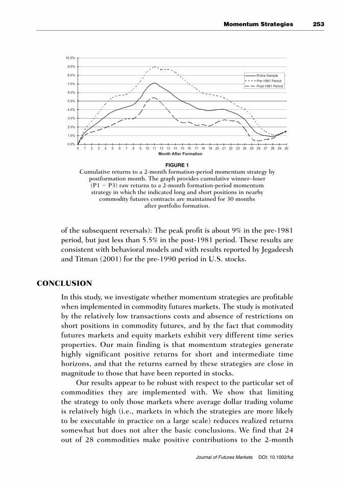
Momentum Strategies 253
Journal of Futures Markets DOI: 10.1002/fut
FIGURE 1Cumulative returns to a 2-month formation-period momentum strategy by
postformation month. The graph provides cumulative winner–loser (P1 � P3) raw returns to a 2-month formation-period momentum strategy in which the indicated long and short positions in nearby
commodity futures contracts are maintained for 30 months after portfolio formation.
Entire Sample
Month After Formation0 1 2 3 4 5 6 7 8 9 10 11 12 13 14 15 16 17 18 19 20 21 22 23 24 25 26 27 28 29 30
10.0%
9.0%
8.0%
7.0%
6.0%
5.0%
4.0%
3.0%
2.0%
1.0%
0.0%
Pre-1981 Period
Post-1981 Period
of the subsequent reversals): The peak profit is about 9% in the pre-1981period, but just less than 5.5% in the post-1981 period. These results areconsistent with behavioral models and with results reported by Jegadeeshand Titman (2001) for the pre-1990 period in U.S. stocks.
CONCLUSION
In this study, we investigate whether momentum strategies are profitablewhen implemented in commodity futures markets. The study is motivatedby the relatively low transactions costs and absence of restrictions onshort positions in commodity futures, and by the fact that commodityfutures markets and equity markets exhibit very different time seriesproperties. Our main finding is that momentum strategies generatehighly significant positive returns for short and intermediate timehorizons, and that the returns earned by these strategies are close inmagnitude to those that have been reported in stocks.
Our results appear to be robust with respect to the particular set ofcommodities they are implemented with. We show that limitingthe strategy to only those markets where average dollar trading volumeis relatively high (i.e., markets in which the strategies are more likelyto be executable in practice on a large scale) reduces realized returnssomewhat but does not alter the basic conclusions. We find that 24out of 28 commodities make positive contributions to the 2-month

254 Shen, Szakmary, and Sharma
Journal of Futures Markets DOI: 10.1002/fut
formation-period momentum strategy. We also show throughout the arti-cle that our results are reasonably robust with respect to the periodexamined (although post-1981 profits, albeit still generally significant,are lower then pre-1981). The robustness of our basic findings acrosstwo very different subperiods suggests that our findings are not solelyattributable to data-snooping biases.
Given the nature of futures markets, where contracts maturefrequently, even longer-term positions must generally be rolled over (andgenerate trading costs) on a monthly basis. Consequently, one questionthat arises is whether the momentum strategies examined here would beprofitable if implemented in real markets. In our judgment, given the esti-mates in Table I, it is extremely unlikely that transactions costs eliminatethe momentum profits documented in this study. Consider the 1-monthholding period strategies applied only to high-volume commodities asreported in Table V, in the post-1981 period during which the returns tothese strategies have been somewhat lower. For the more promisingstrategies that use relatively short formation periods, these returns stillexceed 0.70% per month. Suppose transactions costs, on average, arein the upper-end of the range for the commodities listed in Table I. Astrategy that takes long positions in $10,000,000 worth of commodities(in terms of total contract value) and simultaneous short positions in adifferent set of commodities with the same total contract value, and doesnot require positions to be rolled-over during the 1-month holding period,would incur two sets of transactions costs totaling at most .3% of the$10,000,000 contract value. Moreover, given the relatively high dollartrading volumes in the high-volume subset of commodities, the marketimpact effects of purchasing a total of $10,000,000 contract value ofseven commodities ($1,428,571 per commodity) would be negligible.Thus, even after transactions costs, the strategies simulated here, usedwithout leverage, would earn excess returns (above the T-bill returnsearned on margin deposits) in the range of 0.4%–0.8% per month.
We believe a slightly stronger case can be made that the profitabilityof momentum strategies in commodity futures markets is at least partly dueto risk premia. We show that these strategies lead to significantly higherstandard deviations of realized returns than when long and short posi-tions are assigned randomly, probably because they tend to take positionsin particular commodities precisely at those times when returns in thosecommodities are most volatile. Moreover, the Sharpe ratios earned by arepresentative momentum strategy, while attractive relative to thoseearned on control portfolios, are not out of line with Sharpe ratiosobserved on other asset classes in the post-1981 period. However, when

Momentum Strategies 255
Journal of Futures Markets DOI: 10.1002/fut
we examine the returns to commodity futures in the context of factormodels and implement momentum strategies with risk-adjusted returns,we find that only a relatively small portion of the returns to momentumstrategies can be attributed to systematic risk exposure. In addition,we show that returns to a representative momentum strategy peak11 months after portfolio formation and subsequently reverse. AsJegadeesh and Titman (2001) argue, this last result is most consistentwith behavioral explanations of the momentum phenomenon.
BIBLIOGRAPHY
Barberis, N. C., Shleifer, A., & Vishny, R. W. (1998). A model of investor senti-ment. Journal of Financial Economics, 49, 307–343.
Bessembinder, H., & Chan, K. (1992). Time-varying risk premia and fore-castable returns in futures markets. Journal of Financial Economics, 32,169–194.
Bhardwaj, R. K., & Brooks, L. D. (1992). The January anomaly: Effects of lowshare price, transaction costs, and bid-ask bias. Journal of Finance, 47,553–576.
Chan, K., Hameed, A., & Tong, W. (2000). Profitability of momentum strategiesin the international equity markets. Journal of Financial and QuantitativeAnalysis, 35, 153–172.
Chan, L. K. C., Jegadeesh, N., & Lakonishok, J. (1996). Momentum strategies.Journal of Finance, 51, 1681–1713.
Chen, J., & Hong, H. (2002). Discussion of momentum and autocorrelation instock returns. Review of Financial Studies, 15, 565–573.
Chordia, T., & Shivakumar, L. (2002). Momentum, business cycle, and time-varying expected returns. Journal of Finance, 57, 985–1019.
Conrad, J., & Kaul, G. (1998). An anatomy of trading strategies. Review ofFinancial Studies, 11, 489–519.
Cooper, M. J., Gutierrez, R. C., Jr., & Hameed, A. (2004). Market states andmomentum. Journal of Finance, 59, 1345–1365.
Daniel, K., Hirshleifer, D., & Subrahmanyam, A. (1998). Investor psychologyand security market under- and overreactions. Journal of Finance, 53,1839–1886.
DeBondt, W. F. M., & Thaler, R. (1985). Does the stock market overreact?Journal of Finance, 40, 793–808.
DeBondt, W. F. M., & Thaler, R. (1987). Further evidence of investor overreac-tion and stock market seasonality. Journal of Finance, 42, 557–581.
Fama, E. F., & French, K. R. (1993). Common risk factors in the returns onstocks and bonds. Journal of Financial Economics, 33, 3–56.
Fama, E. F., & French, K. R. (1996). Multifactor explanation of asset pricinganomalies. Journal of Finance, 51, 55–84.
Fleming, J., Ostdiek, B., & Whaley, R. E. (1996). Trading costs and the relativerates of price discovery in stock, futures, and options markets. Journal ofFutures Markets, 16, 353–387.

256 Shen, Szakmary, and Sharma
Journal of Futures Markets DOI: 10.1002/fut
Followill, R. A., & Rodriguez, A. J. (1991). The estimation and determinants ofbid-ask spreads in futures markets. Review of Futures Markets, 10, 1–11.
Fung, W., & Hsieh, D. A. (1997). Survivorship bias and investment style in thereturns of CTAs. Journal of Portfolio Management, 23, 30–41.
George, T. J., & Hwang, C. Y. (2004). The 52-week high and momentum invest-ing. Journal of Finance, 59, 2145–2176.
Griffin, J. M., Ji, X., & Martin, J. S. (2003). Momentum investing and businesscycle risk: Evidence from pole to pole. Journal of Finance, 58, 2515–2547.
Grundy, B. D., & Martin, J. S. (2001). Understanding the nature of the risks andthe source of the rewards to momentum investing. Review of FinancialStudies, 14, 29–78.
Hong, H., Lim, T., & Stein, J. C. (2000). Bad news travels slowly: Size, analystcoverage, and the profitability of momentum strategies. Journal of Finance,55, 265–295.
Irwin, S. H., & Yoshimaru, S. (1999). Managed futures, positive feedback trad-ing, and futures price volatility. Journal of Futures Markets, 19, 759–776.
Jarque, C. M., & Bera, A. K. (1987). A test for normality of observations andregression residuals. International Statistical Review, 55, 163–172.
Jegadeesh, N., & Titman, S. (1993). Returns to buying winners and sellinglosers: Implications for stock market efficiency. Journal of Finance, 48,65–91.
Jegadeesh, N., & Titman, S. (2001). Profitability of momentum strategies: Anevaluation of alternative explanations. Journal of Finance, 56, 699–721.
Jegadeesh, N., & Titman, S. (2002). Cross-sectional and time-series determi-nants of momentum returns. Review of Financial Studies, 15, 143–157.
Korajczyk, R. E., & Sadka, R. (2004). Are momentum profits robust to tradingcosts? Journal of Finance, 59, 1039–1082.
Laux, P. A., & Senchack, A. J., Jr. (1992). Bid-ask spreads In financial futures.Journal of Futures Markets, 12, 621–634.
Lesmond, D. A., Schill, M. J., & Zhou, C. (2004). The illusory nature ofmomentum profits. Journal of Financial Economics, 71, 349–380.
Locke, P. R., & Venkatesh, P. C. (1997). Futures market transaction costs.Journal of Futures Markets, 17, 229–245.
Newey, W. K., & West, K. D. (1987). A simple positive definite, heteroscedas-tocity and autocorrelation consistent covariance matrix. Econometrica, 55,703–708.
Richards, A. J. (1997). Winner-loser reversals in national stock market indices:Can they be explained? Journal of Finance, 52, 2129–2144.
Rouwenhorst, K. G. (1998). International momentum strategies. Journal ofFinance, 53, 267–284.
Stoll, H. R., & Whaley, R. E. (1983). Transaction costs and the small firm effect.Journal of Financial Economics, 12, 57–80.