an evaluation of the measurement requirements for an in ...mln/ltrs-pdfs/nasa-96-tm110218.pdf · 0...

0

NASA Technical Memorandum 110218

An Evaluation of the MeasurementRequirements for an In-Situ Wake VortexDetection System

Henri D. Fuhrmann and Eric C. StewartLangley Research Center, Hampton, Virginia

May 1996

National Aeronautics andSpace AdministrationLangley Research CenterHampton, Virginia 23681-0001

NASA

1

Abstract

Results of a numerical simulation are presented todetermine the feasibility of estimating the location andstrength of a wake vortex from imperfect in-situmeasurements. These estimates could be used toprovide information to a pilot on how to avoid ahazardous wake vortex encounter. An iterativealgorithm based on the method of secants was used tosolve the four simultaneous equations describing thetwo-dimensional flow field around a pair of parallelcounter-rotating vortices of equal and constantstrength. The flow field information used by thealgorithm could be derived from measurements fromflow angle sensors mounted on the wing-tips of thedetecting aircraft and an inertial navigation system.The study determined the propagated errors in theestimated location and strength of the vortex whichresulted from random errors added to theoreticallyperfect measurements. The results are summarized ina series of charts and a table which make it possible toestimate these propagated errors for many practicalsituations. The situations include several generator-detector airplane combinations, different distancesbetween the vortex and the detector airplane, as well asdifferent levels of total measurement error.

Nomenclature

bdet span of the detecting aircraft, ft.bgen span of the generating aircraft, ft.bsep separation distance between the

vortex pair, ft.C numerical method cost function (see

Eqn. 7), deg.M Measurement magnitude of flow field

values (see eqn. 8), deg.r radius from the center of a vortex to the

point of calculation (eqn. 3A), ft.R radius from the center of a vortex

dipole to the point of calculation, ft.

AN EVALUATION OF THE MEASUREMENT REQUIREMENTS FOR AN IN-SITU WAKE VORTEXDETECTION SYSTEM

Henri D. FuhrmannEric C. Stewart

NASA Langley Research CenterHampton, Virginia 23681-0001

Vgen velocity of the generating aircraft, ft./sec.Vdet velocity of the detecting aircraft, ft./sec.vθ tangential velocity component at radius

(r) of a vortex, ft./sec.v horizontal velocity component of

the vortex flow field (eqn. 4), ft./sec. ordeg.

videal theoretical horizontal velocitycomponent of vortex flow field, ft./sec.

Wgen weight of the generating aircraft, lb.w vertical velocity component of the

vortex flow field (eqn. 3), deg.wideal theoretical vertical velocity component

of vortex flow field, ft./sec.y horizontal position of the detecting

aircraft, ft.z vertical position of the detecting aircraft,

ft.α angle of attack at one wing tip due to

one vortex, radiansβ angle of sideslip on one wing tip due to

one vortex, radians∆α differential angle of attack across span of

detector airplane due to vortex, deg.∆β differential sideslip angle across span of

detector airplane due to vortex, deg.ε∆α Error for ∆α flow field value, deg.ε∆β Error for ∆β flow field value, deg.εw Error for (w) flow field value, deg.εv Error for (v) flow field value, deg.εtotal Total flow field error (see eqn. 5), deg.Γ circulation strength of the vortex, ft.2/

sec.φ roll angle of the detecting aircraft, deg.ρ air density, slug/ft3.)θ angle from the center of a vortex to a

point of calculation, deg.Subscriptsi=1, 2, or 3 indicating the right wing tip, left wing

tip, and centerline respectively.

2

j=1 or 2 indicating the right and left vortexrespectively.

ideal theoretical value with no measurementerror

c calculated value based on estimatedvortex parameters

Abbreviations:FAA Federal Aviation AdministrationIFR Instrument Flight RuleIMC Instrument Meteorological Conditionsmax maximum value

Introduction

Recent studies have highlighted the costly airlinedelays at major airports due to limited airport capacityand air traffic congestion.1 One factor contributing tothese delays is the longitudinal spacing requirementbetween aircraft on approach to landing imposed bythe Federal Aviation Administration (FAA) inInstrument Meteorological Conditions (IMC). Thesespacing requirements were defined so as to reduce thelikelihood of hazardous wake vortex encounters byaircraft during takeoff and on approach to landing.Recognizing these separation requirements as a sourceof air traffic delays, the FAA has prompted areevaluation of these standards. If the separationdistances can safely be reduced a reduction in airportcongestion and delays would ensue. A reduction inseparation requirements is estimated to have apotential billion dollar a year savings for the nation’sairlines.2 Reduction of the spacing requirements,however, must be approached cautiously as severalrecent airplane incidents have been attributed to wakevortex disturbances.3

In the past, much effort was devoted to reducing thevortex hazard by modifying geometry or procedures ofthe airplane generating the vortex so as to attenuate thevortex to a level deemed safe4. However, none of thesemodifications have yet been shown to be practical5.More recently NASA has been studying means toincrease airport capacity by predicting or sensingweather conditions when it will be safe to reduce thespacing requirements. An Aircraft Vortex SpacingSystem (AVOSS) has been proposed which will usemeasurements of weather conditions to predict whenvortices will have decayed to a safe level or blown outof the approach corridor6. Although the AVOSS system

will use ground-based measurements, air-bornemeasurements could also be useful. Airborne detectionschemes may take the form of a modified windsheardetection system using Doppler RADAR7, or aerosolmotion and velocity determination via Light Detectionand Ranging (LIDAR). An alternate system using flowangle sensors and an inertial navigation system hasbeen suggested. This study evaluates the concept ofsuch a system to see if it could be sensitive enough toprovide the pilot with information to allow evasivemaneuvers to be executed.

Exploratory test flights have demonstrated thepossibility of detecting wake vortices at substantiallateral distances with simple, low-cost wing tip flowmonitoring devices.8 Though no attempt to locate thevortex pair or to determine the vortex strength wasperformed in this study, the results show that adequatedetection and maneuver time may be available.

Further analysis by Stewart9 of this joint FAA/NASAflight test has revealed that flow angles alone are notsufficient for a unique determination of detectingaircraft location with respect to a vortex pair as hadbeen previously theorized10. Additional informationderived from inertial velocity measurements is alsoneeded. With these measurements vortex velocitiesand velocity gradients can be determined.

Assuming the correct model of the vortex flow field isknown, the strength and location of a wake vortex canbe determined using exact measurements of thevelocities and velocity gradients in the flow field.However, if the model is not correct or if themeasurements are not perfect, the estimated locationand strength of the wake vortex will be in error. Theprimary purpose of this paper is to determine howerrors in the measurements propagate into errors in theestimated strength and location values determined forthe wake vortex. With this information, the allowablemeasurement error can be determined for such asystem to be feasible. The measurement error is acombination of instrumentation noise, atmosphericturbulence, and contamination due to aircraft motion.

The question of the correctness of the mathematicalmodel of the wake vortex will not be addressed herein.For this paper, simulated data with known amounts oferror will be used to evaluate the error propagationrelationships using an iterative algorithm developed

3

for this study. The axes of the airplane are assumed tobe aligned with the axes of the wake vortex allowing forthe two-dimensional problem to be studied here. Thealgorithm is described and typical convergence ratesare presented for different trajectories andmeasurement errors. The results are summarized in aseries of charts and a table which make it possible toestimate these propagated errors for many practicalsituations. The situations include several generator-detector airplane combinations, different distancesbetween the vortex and the detector airplane, as well asdifferent levels of total measurement error.

Theory

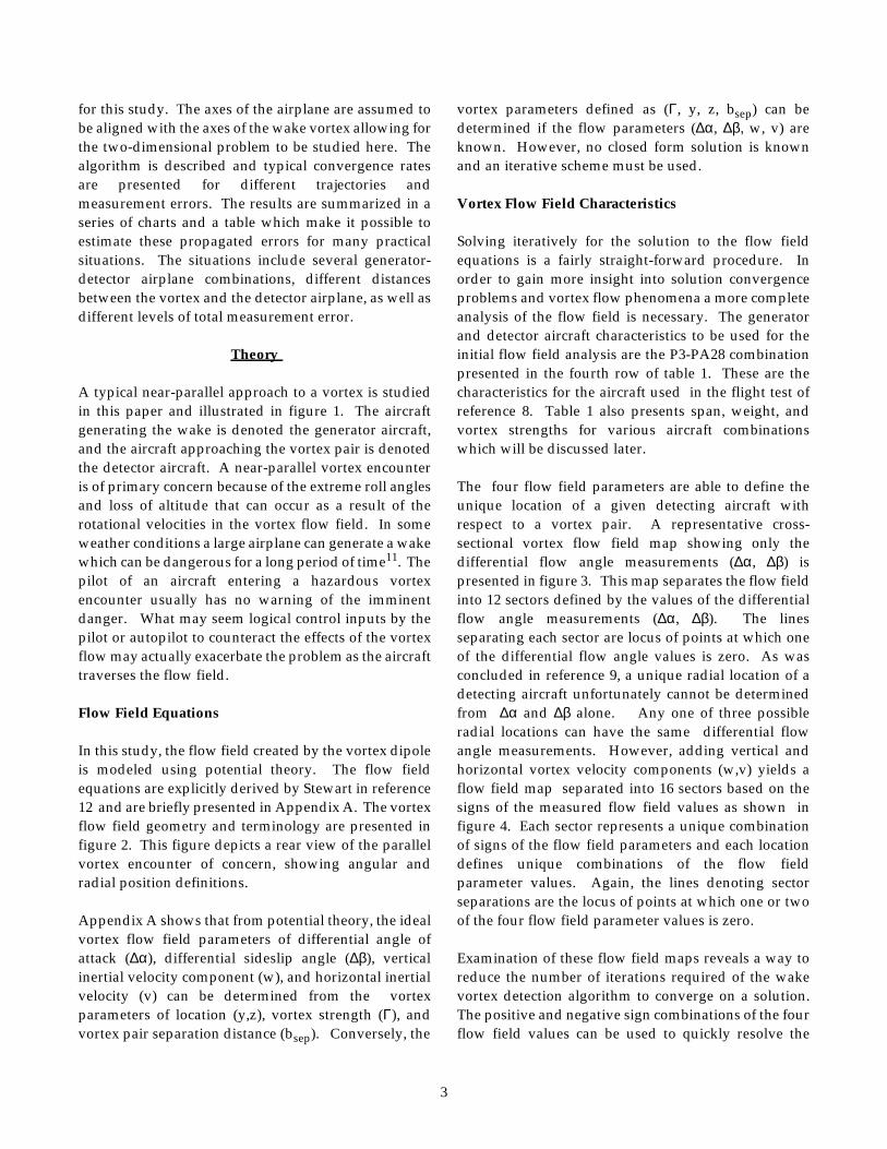
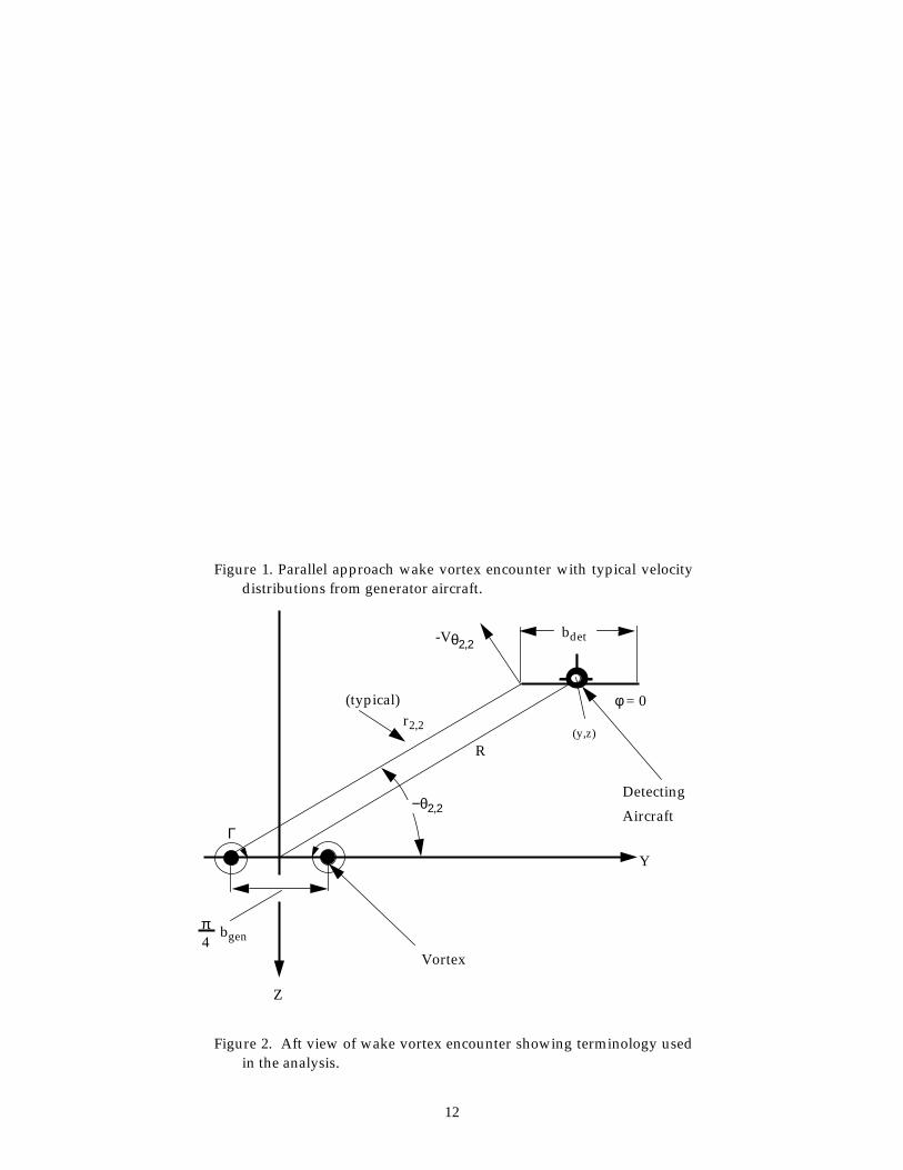
A typical near-parallel approach to a vortex is studiedin this paper and illustrated in figure 1. The aircraftgenerating the wake is denoted the generator aircraft,and the aircraft approaching the vortex pair is denotedthe detector aircraft. A near-parallel vortex encounteris of primary concern because of the extreme roll anglesand loss of altitude that can occur as a result of therotational velocities in the vortex flow field. In someweather conditions a large airplane can generate a wakewhich can be dangerous for a long period of time11. Thepilot of an aircraft entering a hazardous vortexencounter usually has no warning of the imminentdanger. What may seem logical control inputs by thepilot or autopilot to counteract the effects of the vortexflow may actually exacerbate the problem as the aircrafttraverses the flow field.

Flow Field Equations

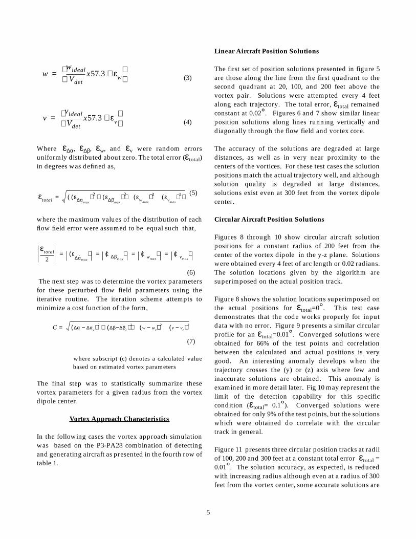
In this study, the flow field created by the vortex dipoleis modeled using potential theory. The flow fieldequations are explicitly derived by Stewart in reference12 and are briefly presented in Appendix A. The vortexflow field geometry and terminology are presented infigure 2. This figure depicts a rear view of the parallelvortex encounter of concern, showing angular andradial position definitions.

Appendix A shows that from potential theory, the idealvortex flow field parameters of differential angle ofattack (∆α), differential sideslip angle (∆β), verticalinertial velocity component (w), and horizontal inertialvelocity (v) can be determined from the vortexparameters of location (y,z), vortex strength (Γ), andvortex pair separation distance (bsep). Conversely, the

vortex parameters defined as (Γ, y, z, bsep) can bedetermined if the flow parameters (∆α, ∆β, w, v) areknown. However, no closed form solution is knownand an iterative scheme must be used.

Vortex Flow Field Characteristics

Solving iteratively for the solution to the flow fieldequations is a fairly straight-forward procedure. Inorder to gain more insight into solution convergenceproblems and vortex flow phenomena a more completeanalysis of the flow field is necessary. The generatorand detector aircraft characteristics to be used for theinitial flow field analysis are the P3-PA28 combinationpresented in the fourth row of table 1. These are thecharacteristics for the aircraft used in the flight test ofreference 8. Table 1 also presents span, weight, andvortex strengths for various aircraft combinationswhich will be discussed later.

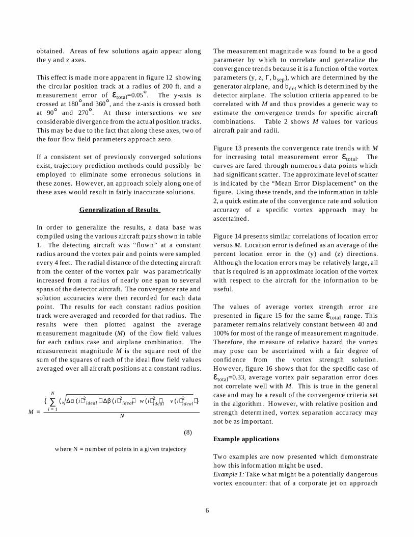
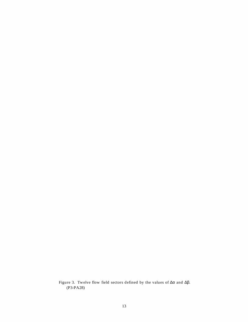
The four flow field parameters are able to define theunique location of a given detecting aircraft withrespect to a vortex pair. A representative cross-sectional vortex flow field map showing only thedifferential flow angle measurements (∆α, ∆β) ispresented in figure 3. This map separates the flow fieldinto 12 sectors defined by the values of the differentialflow angle measurements (∆α, ∆β). The linesseparating each sector are locus of points at which oneof the differential flow angle values is zero. As wasconcluded in reference 9, a unique radial location of adetecting aircraft unfortunately cannot be determinedfrom ∆α and ∆β alone. Any one of three possibleradial locations can have the same differential flowangle measurements. However, adding vertical andhorizontal vortex velocity components (w,v) yields aflow field map separated into 16 sectors based on thesigns of the measured flow field values as shown infigure 4. Each sector represents a unique combinationof signs of the flow field parameters and each locationdefines unique combinations of the flow fieldparameter values. Again, the lines denoting sectorseparations are the locus of points at which one or twoof the four flow field parameter values is zero.

Examination of these flow field maps reveals a way toreduce the number of iterations required of the wakevortex detection algorithm to converge on a solution.The positive and negative sign combinations of the fourflow field values can be used to quickly resolve the

4

angular location of a detecting aircraft with respect tothe vortex pair. This sector location method was usedto provide initial estimates of the solution parameters(y, z). However, the existence of a vortex was notconsidered to be established until a converged solutionwas obtained using the iterative algorithm.

Wake Vortex Location Algorithm

The wake vortex detection and location algorithm iscomposed of (1) an initialization routine, (2) vortex flowfield equations module, and (3) an iterative scheme forconverging on the estimate of the vortex parameters.This algorithm is explained in more detail in appendixB.

The code was compiled and run on various systems.The results of this study are from a SUN IPX with afixed computational power of 28.5 MIPS or 4.2MFLOPS.

Error Evaluation Procedure

This section describes the procedure used to evaluatethe effects of measurement error on the accuracy of thevortex parameter solution. The detecting airplane was

assumed to be traveling in the same general direction asthe axis of the wake vortex but with small velocities inthe plane perpendicular to the axis. The span (bdet),velocity (Vdet), and roll attitude (φ) of the detectingaircraft are taken to be known quantities. For simplicityin this study, the roll angle of the detecting aircraft isfixed at zero.

The first step was to calculate a series of ideal flow fieldvalues (∆αideal, ∆βideal, wideal, videal) along a giventrajectory with an assumed set of vortex parameters.This assumed set of vortex parameters was retained forcomparison with estimated vortex parameters.

The second step was to add random errors to the idealflow field parameters as shown in the followingequations.

(1)

(2)

∆α ∆αideal ε∆α+=

∆β ∆βideal ε∆β+=

Table 1: Aircraft pairs and characteristics (Vgen=Vdet=200 ft./sec.)

Aircraft Pairs(Generator-Detector)

bgen-bdetft.

Wgen-Wdetlb.

Γgenft2./sec.

737-737 94.8 - 94.8 114,000 - 114,000 3840

MD11-MD80 169.5 - 108 430,000 - 128,000 8075

747-737 211 - 94.8 574,000 - 114,000 8659

P3-PA28 100.3 - 34.5 95,500 - 2,200 2494

757-Citation 124.8 - 53.5 198,000 - 20,000 5050

757-737 124.8 - 94.8 198,000 - 114,000 5050

757-C182 124.8 - 40 198,000 - 3,500 5050

757-Corporate Jet 124.8 - 43.8 198,000 - 18,000 5050

757(heavy)-Corporate jet 124.8 - 43.8 217,348 - 18,000 5543

MD11(mod)-MD80 169.5 - 108 395,044 - 128,000 7418

5

(3)

(4)

Where ε∆α, ε∆β, εw, and εv were random errorsuniformly distributed about zero. The total error (εtotal)in degrees was defined as,

(5)

where the maximum values of the distribution of eachflow field error were assumed to be equal such that,

(6) The next step was to determine the vortex parametersfor these perturbed flow field parameters using theiterative routine. The iteration scheme attempts tominimize a cost function of the form,

(7)

where subscript (c) denotes a calculated valuebased on estimated vortex parameters

The final step was to statistically summarize thesevortex parameters for a given radius from the vortexdipole center.

Vortex Approach Characteristics

In the following cases the vortex approach simulationwas based on the P3-PA28 combination of detectingand generating aircraft as presented in the fourth row oftable 1.

wwideal

Vdetx57.3 εw+

=

vvideal

Vdetx57.3 εv+

=

εtotal ε∆αmax( ) 2 ε∆βmax

( ) 2 εwmax( ) 2 εvmax

( ) 2+ + +( )=

εtotal

2ε

∆α̇max

( ) ε∆βmax( ) εwmax

( ) εvmax( )= = = =

C ∆α ∆αc−( ) 2∆β ∆− βc( ) 2

w wc−( ) 2v vc−( ) 2+ + +=

Linear Aircraft Position Solutions

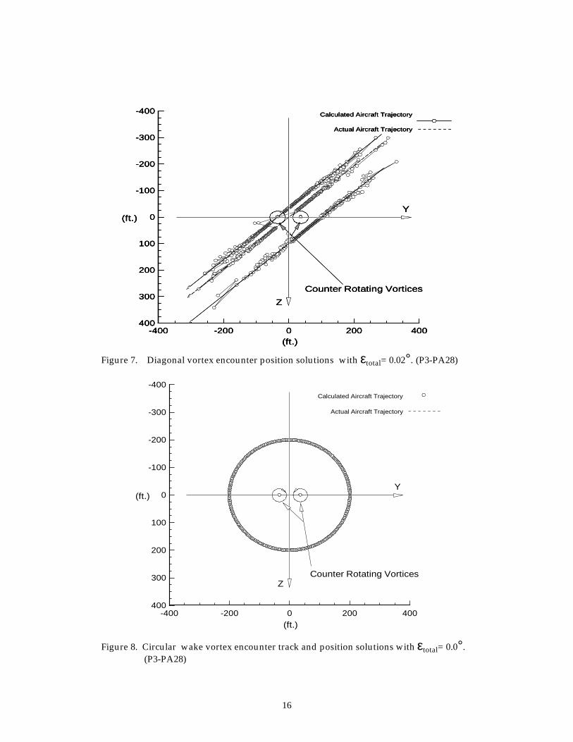
The first set of position solutions presented in figure 5are those along the line from the first quadrant to thesecond quadrant at 20, 100, and 200 feet above thevortex pair. Solutions were attempted every 4 feetalong each trajectory. The total error, εtotal remainedconstant at 0.02°. Figures 6 and 7 show similar linearposition solutions along lines running vertically anddiagonally through the flow field and vortex core.

The accuracy of the solutions are degraded at largedistances, as well as in very near proximity to thecenters of the vortices. For these test cases the solutionpositions match the actual trajectory well, and althoughsolution quality is degraded at large distances,solutions exist even at 300 feet from the vortex dipolecenter.

Circular Aircraft Position Solutions

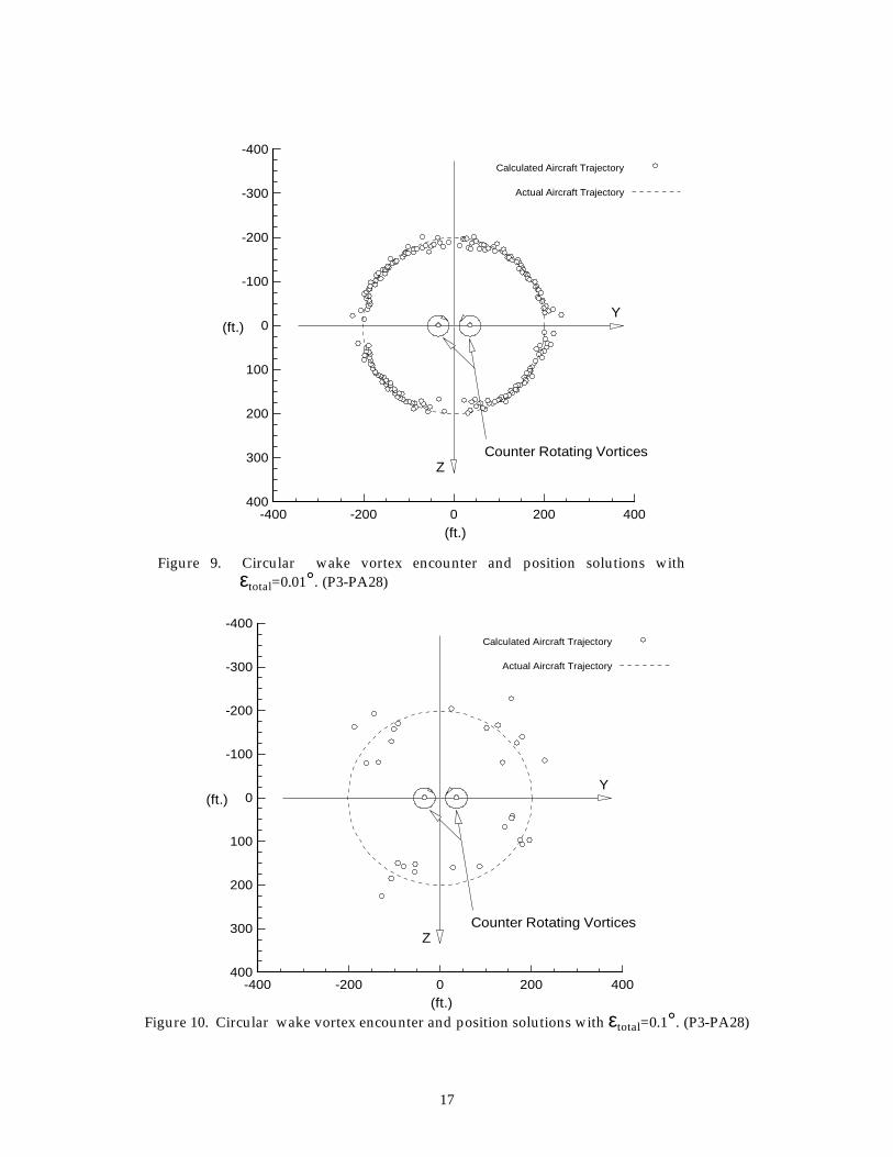
Figures 8 through 10 show circular aircraft solutionpositions for a constant radius of 200 feet from thecenter of the vortex dipole in the y-z plane. Solutionswere obtained every 4 feet of arc length or 0.02 radians.The solution locations given by the algorithm aresuperimposed on the actual position track.

Figure 8 shows the solution locations superimposed onthe actual positions for εtotal=0°. This test casedemonstrates that the code works properly for inputdata with no error. Figure 9 presents a similar circularprofile for an εtotal=0.01°. Converged solutions wereobtained for 66% of the test points and correlationbetween the calculated and actual positions is verygood. An interesting anomaly develops when thetrajectory crosses the (y) or (z) axis where few andinaccurate solutions are obtained. This anomaly isexamined in more detail later. Fig 10 may represent thelimit of the detection capability for this specificcondition (εtotal= 0.1°). Converged solutions wereobtained for only 9% of the test points, but the solutionswhich were obtained do correlate with the circulartrack in general.

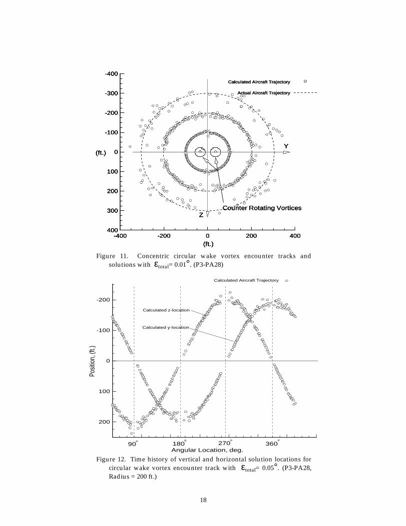
Figure 11 presents three circular position tracks at radiiof 100, 200 and 300 feet at a constant total error εtotal =0.01°. The solution accuracy, as expected, is reducedwith increasing radius although even at a radius of 300feet from the vortex center, some accurate solutions are

6

obtained. Areas of few solutions again appear alongthe y and z axes.

This effect is made more apparent in figure 12 showingthe circular position track at a radius of 200 ft. and ameasurement error of εtotal=0.05°. The y-axis iscrossed at 180°and 360°, and the z-axis is crossed bothat 90° and 270°. At these intersections we seeconsiderable divergence from the actual position tracks.This may be due to the fact that along these axes, two ofthe four flow field parameters approach zero.

If a consistent set of previously converged solutionsexist, trajectory prediction methods could possibly beemployed to eliminate some erroneous solutions inthese zones. However, an approach solely along one ofthese axes would result in fairly inaccurate solutions.

Generalization of Results

In order to generalize the results, a data base wascompiled using the various aircraft pairs shown in table1. The detecting aircraft was “flown” at a constantradius around the vortex pair and points were sampledevery 4 feet. The radial distance of the detecting aircraftfrom the center of the vortex pair was parametricallyincreased from a radius of nearly one span to severalspans of the detector aircraft. The convergence rate andsolution accuracies were then recorded for each datapoint. The results for each constant radius positiontrack were averaged and recorded for that radius. Theresults were then plotted against the averagemeasurement magnitude (M) of the flow field valuesfor each radius case and airplane combination. Themeasurement magnitude M is the square root of thesum of the squares of each of the ideal flow field valuesaveraged over all aircraft positions at a constant radius.

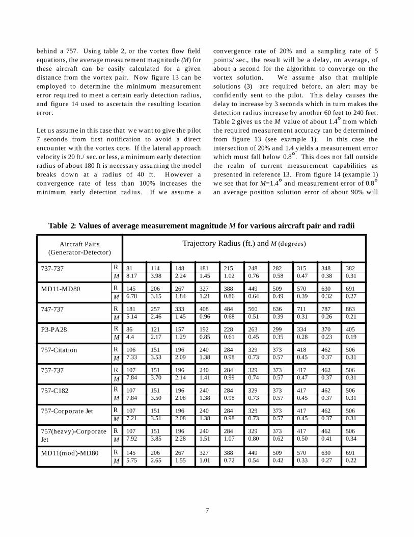
The measurement magnitude was found to be a goodparameter by which to correlate and generalize theconvergence trends because it is a function of the vortexparameters (y, z, Γ, bsep), which are determined by thegenerator airplane, and bdet which is determined by thedetector airplane. The solution criteria appeared to becorrelated with M and thus provides a generic way toestimate the convergence trends for specific aircraftcombinations. Table 2 shows M values for variousaircraft pair and radii.

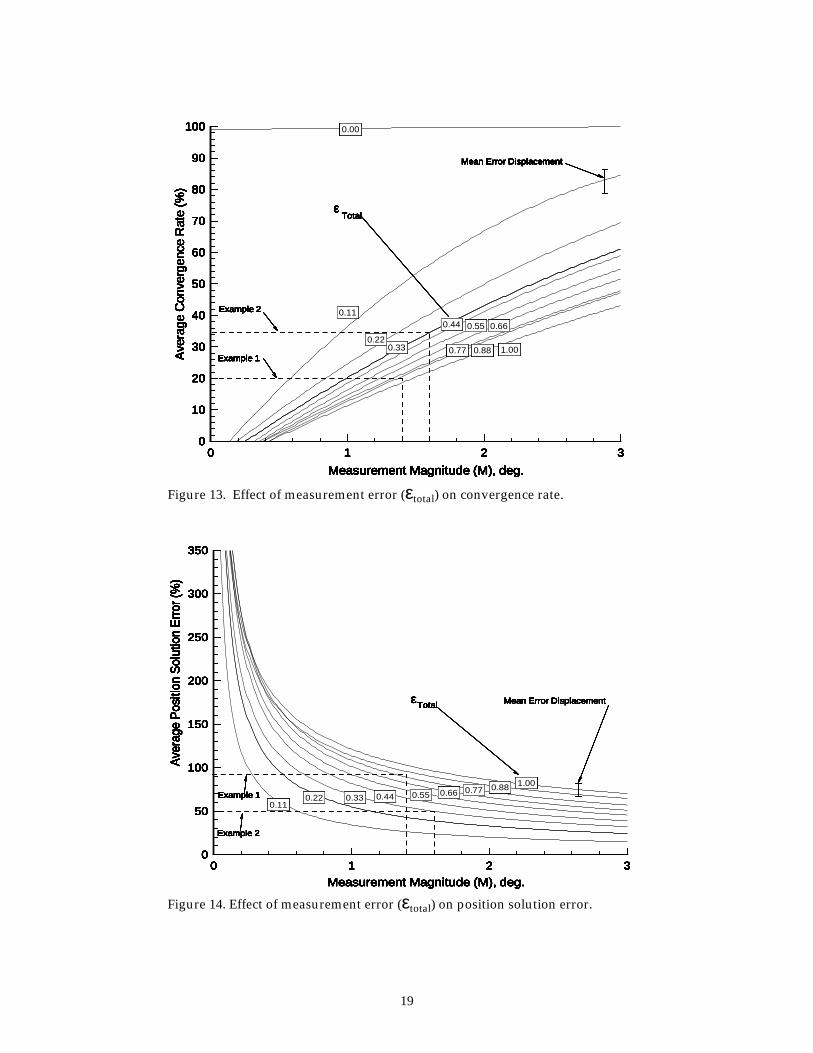
Figure 13 presents the convergence rate trends with Mfor increasing total measurement error εtotal. Thecurves are fared through numerous data points whichhad significant scatter. The approximate level of scatteris indicated by the “Mean Error Displacement” on thefigure. Using these trends, and the information in table2, a quick estimate of the convergence rate and solutionaccuracy of a specific vortex approach may beascertained.

Figure 14 presents similar correlations of location errorversus M. Location error is defined as an average of thepercent location error in the (y) and (z) directions.Although the location errors may be relatively large, allthat is required is an approximate location of the vortexwith respect to the aircraft for the information to beuseful.

The values of average vortex strength error arepresented in figure 15 for the same εtotal range. Thisparameter remains relatively constant between 40 and100% for most of the range of measurement magnitude.Therefore, the measure of relative hazard the vortexmay pose can be ascertained with a fair degree ofconfidence from the vortex strength solution.However, figure 16 shows that for the specific case ofεtotal=0.33, average vortex pair separation error doesnot correlate well with M. This is true in the generalcase and may be a result of the convergence criteria setin the algorithm. However, with relative position andstrength determined, vortex separation accuracy maynot be as important.

Example applications

Two examples are now presented which demonstratehow this information might be used.Example 1: Take what might be a potentially dangerousvortex encounter: that of a corporate jet on approach

(8)

where N = number of points in a given trajectory

M

∆α i( ) 2ideal ∆β i( ) 2

ideal w i( ) ideal2 v i( ) ideal

2+ + +( )i 1=

N

∑{ }

N=

7

behind a 757. Using table 2, or the vortex flow fieldequations, the average measurement magnitude (M) forthese aircraft can be easily calculated for a givendistance from the vortex pair. Now figure 13 can beemployed to determine the minimum measurementerror required to meet a certain early detection radius,and figure 14 used to ascertain the resulting locationerror.

Let us assume in this case that we want to give the pilot7 seconds from first notification to avoid a directencounter with the vortex core. If the lateral approachvelocity is 20 ft./sec. or less, a minimum early detectionradius of about 180 ft is necessary assuming the modelbreaks down at a radius of 40 ft. However aconvergence rate of less than 100% increases theminimum early detection radius. If we assume a

convergence rate of 20% and a sampling rate of 5points/sec., the result will be a delay, on average, ofabout a second for the algorithm to converge on thevortex solution. We assume also that multiplesolutions (3) are required before, an alert may beconfidently sent to the pilot. This delay causes thedelay to increase by 3 seconds which in turn makes thedetection radius increase by another 60 feet to 240 feet.Table 2 gives us the M value of about 1.4° from whichthe required measurement accuracy can be determinedfrom figure 13 (see example 1). In this case theintersection of 20% and 1.4 yields a measurement errorwhich must fall below 0.8°. This does not fall outsidethe realm of current measurement capabilities aspresented in reference 13. From figure 14 (example 1)we see that for M=1.4° and measurement error of 0.8°an average position solution error of about 90% will

Table 1: Values of average measurement magnitudeM for various aircraft pair and radii

Aircraft Pairs(Generator-Detector)

Trajectory Radius (ft.) andM (degrees)

737-737 818.17

1143.98

1482.24

1811.45

2151.02

2480.76

2820.58

3150.47

3480.38

3820.31

MD11-MD80 1456.78

2063.15

2671.84

3271.21

3880.86

4490.64

5090.49

5700.39

6300.32

6910.27

747-737 1815.14

2572.46

3331.45

4080.96

4840.68

5600.51

6360.39

7110.31

7870.26

8630.21

P3-PA28 864.4

1212.17

1571.29

1920.85

2280.61

2630.45

2990.35

3340.28

3700.23

4050.19

757-Citation 1067.33

1513.53

1962.09

2401.38

2840.98

3290.73

3730.57

4180.45

4620.37

5060.31

757-737 1077.84

1513.70

1962.14

2401.41

2840.99

3290.74

3730.57

4170.47

4620.37

5060.31

757-C182 1077.84

1513.50

1962.08

2401.38

2840.98

3290.73

3730.57

4170.45

4620.37

5060.31

757-Corporate Jet 1077.21

1513.51

1962.08

2401.38

2840.98

3290.73

3730.57

4170.45

4620.37

5060.31

757(heavy)-CorporateJet

1077.92

1513.85

1962.28

2401.51

2841.07

3290.80

3730.62

4170.50

4620.41

5060.34

MD11(mod)-MD80 1455.75

2062.65

2671.55

3271.01

3880.72

4490.54

5090.42

5700.33

6300.27

6910.22

RM

RM

RM

RM

RM

RM

RM

RM

RM

RM

2

8

result. In summary, given the convergence raterequired for early detection and avoidance, ameasurement requirement and resulting solution errorcan be determined.

Example 2: Conversely, the avoidance time which can beprovided the pilot can be estimated from themeasurement error and allowable convergence rate. Ifone can measure the vortex flow with an accuracy of0.33° (εtotal=0.33) and tolerate a 50% error in thesolution location, then they can detect a vortex with ameasurement magnitude (M) of 1.6° (fig. 14 example 2).This would have a convergence rate of approximately35% (fig. 13). If one assumes a 747-737 combination ofaircraft, this would correspond to a detection range ofabout 322 ft. (table 2). Assuming a closure rate of 20 feetper second, this would allow a pilot about 16 seconds toreact from first alarm.

False Solutions

The probability that turbulence will cause the algorithmto converge on a false solution should be small. In otherwords, the algorithm should not ordinarily convergefor measured values that do not have the uniquesignature of a vortex flow field. In this way the codewould act as a filter against false alarms.

Algorithm testing on random turbulent flow fieldmeasurements showed that the code produces a falsesolution on turbulent values only 0.2% of the time.That is, the algorithm will “accidently” converge on asolution for a vortex flow field when given randomturbulence measurement on average two out of every1000 sampled points. This rate is probably acceptable ifseveral consistent and consecutive solutions arerequired before an alarm is issued.

Concluding Remarks

A numerical simulation has been made to study thefeasibility of using in-situ measurements to determinethe location and strength of a wake vortex. Simulatedmeasurements with different levels of noise or errorwere used to estimate the vortex location and strengthusing an iterative algorithm. The algorithm is intendedfor a pilot alarm which should be effective for slowencounter rates such as those which occur in near-parallel vortex encounters on landing approach. Thespecific conclusions of the present study are as follows:

1) The algorithm can provide reasonable estimates ofvortex location and strength using simulatedmeasurements with moderate amounts of error.

2) The quality of the estimates of the vortexcharacteristics and location decrease with increasingmeasurement error and distance from the vortex. Thequality of the estimates was also poor in near proximityto the vortex pair.

3) The convergence rate of the algorithm decreasedwith increasing distance and error.

4) There are regions of the vortex field in which thevortex estimates are degraded independent of distanceform the vortex.

5) The algorithm produces very few false solutions insimulated random turbulence and thus provides aneffective filter against false alarms.

6) Tables and graphs are presented for severalcontemporary airplanes which provide a rapid meansto estimate requirements for measurement error toachieve a specified convergence rate and solutionaccuracy.

7) The concept appears to provide the possibility ofdetecting, locating, and estimating the strength of avortex at a distance which could provide a pilot withample time to make an evasive maneuver for near-parallel encounters.

References

1. Page, Richard: The Wake Vortex Problem Revisited. Inproceedings for Radio Technical Commission forAeronautics Annual Assembly and TechnicalSymposium, December 1989.

2. Baart, Douglas; Monk, Helen; and Schweiker, Mary:Airport Capacity and Delay Analyses. U.S. Department ofTransportation/Federal Aviation Administration,DOT/FAA/CT-TN91/18, April 1991.

3. Warwick, Graham: “FAA Questions 757 VortexSeparation.” Flight International, January 18, 1994.

4. Rossow, Vernon J.: Prospects for Alleviation of HazardPosed by Lift-Generated Wakes. Proceedings of Aircraft

9

Appendix A: Flow Field Equations

The assumptions used in the testing of the detectionalgorithm are: (1) the vortices remain parallel to each otherand the ground plane, (2) strength is constant with time (nodecay), (3) the vortex strength (Γ) and separation (bsep) aregiven by eqns. 1A and 2A respectively which are derivedassuming an elliptical lift distribution, (4) the effect of thedetecting aircraft on the vortex flow field is assumed to benegligible, and (5) the longitudinal axis of the detectingaircraft is assumed to be parallel to the vortex pair.

The 2-dimensional vortex flow field geometry andterminology used herein are presented in figure 2. Thisfigure depicts a rear view of the parallel vortex encounter ofconcern, showing angular and radial position definitions.

(1A)

(2A)

(3A)

The tangential velocity component (equation 3A) of the jth

vortex is resolved into vertical and horizontal velocities atthe location of the ith wing-tip of the detecting aircraft.These velocity components are then used to calculate thevortex induced angle of attack αi,j and angle of sideslip βi,jusing a small angle approximation.

(4A)

(5A)

Where the subscript (i) being either the number1 or 2 representing the right or left wing tiprespectively, and (j) is the number 1 or 2referring to the right or left vortex.

Γ 4π

Wgen

ρ Vgen bgen× × =

vθi j,

Γ2πr i j,

=

bsepπ4

bgen×=

αi j,

vθi j,Vdet

{ } θi j, φ θi j, φsinsin−coscos{ }=

βi j,

vθi j,Vdet

{ } θi j, φ θi j, φsincos+cossin{ }=

Wake Vortices Conference, DOT/FAA/SD-92/1.1 orDOT-VNTSC-FAA-92-7.1, Washington, D.C. October29-31, 1991.

5. Dunham, R. E., Jr.: Unsuccessful Concepts for AircraftWake Vortex Minimization. Wake Vortex Minimization,NASA SP-409, 1977, pp. 221-249.

6. Hinton, D. A.: Aircraft Vortex Spacing System(AVOSS) Conceptual Design. NASA TM 110184, August1995.

7. Nespor, J. D., Hudson, B., Stegall, R. L., andFreedman, J. E.: Doppler Radar Detection of Vortex HazardIndicators. Proceedings of Aircraft Wake VorticesConference, DOT/FAA/SD-92/1.1 or DOT-VNTSC-FAA-92-7.1, Washington, D.C. October 29-31, 1991.

8. Branstetter, J. R.; Hastings, E. C.; and Patterson, J. C.Jr.: Flight Test to Determine Feasibility of a ProposedAirborne Wake Vortex Detection Concept. DOT/FAA/CT-TN 90/25, NASA TM 102672, April 1991.

9. Stewart, Eric C.: A Comparison of Airborne Wake VortexDetection Measurements with Values Predicted from SimpleTheory. NASA TP 3125, November 1991.

10. Bilanin, Alan J.; Milton, Teske E.; and Curtiss,Howard C. Jr.: Feasibility of an Onboard Wake VortexAvoidance System. NASA CR 187521, April 1987.

11. Olsen, Goldburg, and Rogers, Aircraft WakeTurbulence, and its Detection, 1990.

12. Stewart, Eric C.: Flight-Test Evaluation of a Direct-Measurement Airborne Wake-Vortex Detection Concept.Proceedings of Aircraft Wake Vortices Conference,DOT/FAA/SD-92/1.1 or DOT-VNTSC-FAA-92-7.1,Washington, D.C. October 29-31, 1991.

13. Scott, M. A.; Strain, N. A.; Lee, C. C.: FlightEvaluation of a Stagnation Detection Hot-Film Sensor.AIAA Paper 92-4085, August, 1992.

14. Burden, Richard L.; and Faires, J. Douglas:Numerical Analysis. PWS Publishing Company, Boston,1993.

10

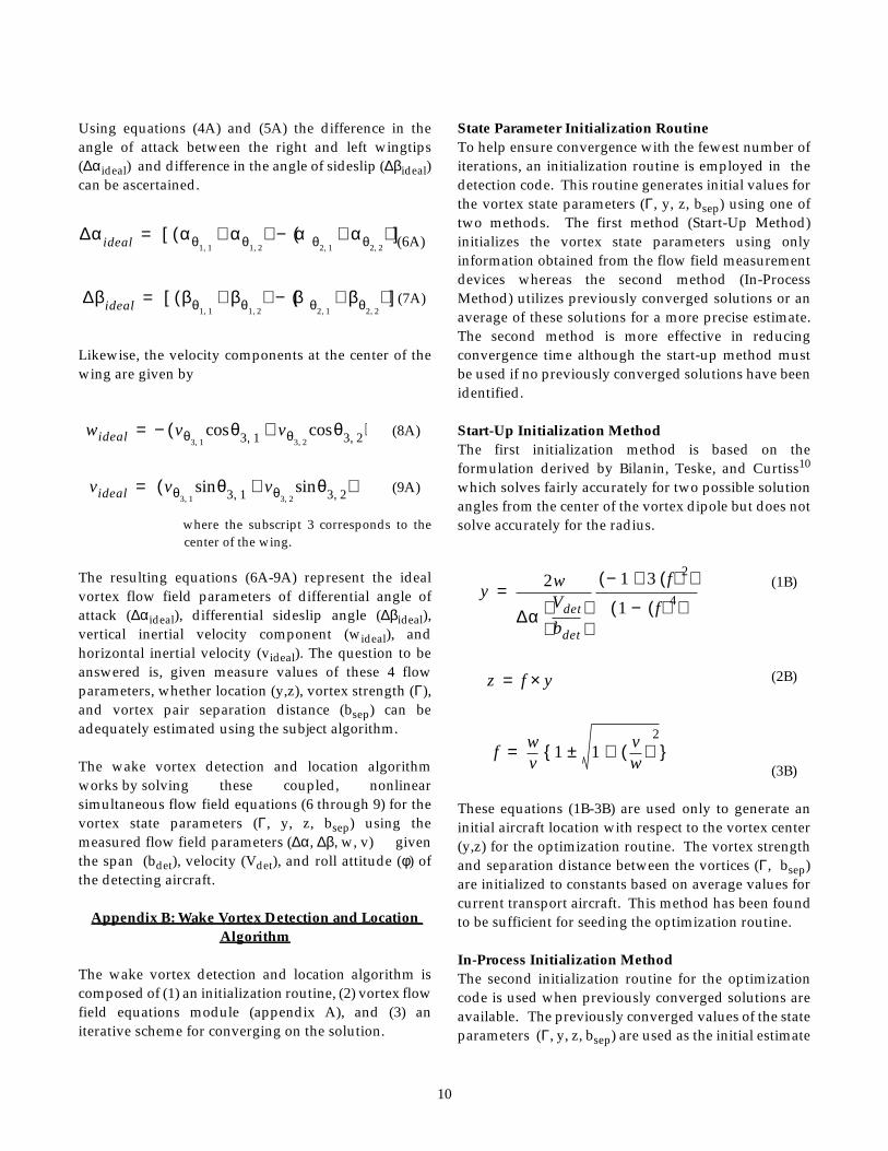
Using equations (4A) and (5A) the difference in theangle of attack between the right and left wingtips(∆αideal) and difference in the angle of sideslip (∆βideal)can be ascertained.

(6A)

(7A)

Likewise, the velocity components at the center of thewing are given by

(8A)

(9A)

where the subscript 3 corresponds to thecenter of the wing.

The resulting equations (6A-9A) represent the idealvortex flow field parameters of differential angle ofattack (∆αideal), differential sideslip angle (∆βideal),vertical inertial velocity component (wideal), andhorizontal inertial velocity (videal). The question to beanswered is, given measure values of these 4 flowparameters, whether location (y,z), vortex strength (Γ),and vortex pair separation distance (bsep) can beadequately estimated using the subject algorithm.

The wake vortex detection and location algorithmworks by solving these coupled, nonlinearsimultaneous flow field equations (6 through 9) for thevortex state parameters (Γ, y, z, bsep) using themeasured flow field parameters (∆α, ∆β, w, v) giventhe span (bdet), velocity (Vdet), and roll attitude (φ) ofthe detecting aircraft.

Appendix B: Wake Vortex Detection and LocationAlgorithm

The wake vortex detection and location algorithm iscomposed of (1) an initialization routine, (2) vortex flowfield equations module (appendix A), and (3) aniterative scheme for converging on the solution.

∆αideal αθ1 1,αθ1 2,

+( ) αθ2 1,αθ2 2,

+( )−[ ]=

∆βideal βθ1 1,βθ1 2,

+( ) βθ2 1,βθ2 2,

+( )−[ ]=

wideal vθ3 1,θ3 1,cos vθ3 2,

θ3 2,cos+( )−=

videal vθ3 1,θ3 1,sin vθ3 2,

θ3 2,sin+( )=

State Parameter Initialization RoutineTo help ensure convergence with the fewest number ofiterations, an initialization routine is employed in thedetection code. This routine generates initial values forthe vortex state parameters (Γ, y, z, bsep) using one oftwo methods. The first method (Start-Up Method)initializes the vortex state parameters using onlyinformation obtained from the flow field measurementdevices whereas the second method (In-ProcessMethod) utilizes previously converged solutions or anaverage of these solutions for a more precise estimate.The second method is more effective in reducingconvergence time although the start-up method mustbe used if no previously converged solutions have beenidentified.

Start-Up Initialization MethodThe first initialization method is based on theformulation derived by Bilanin, Teske, and Curtiss10

which solves fairly accurately for two possible solutionangles from the center of the vortex dipole but does notsolve accurately for the radius.

(1B)

(2B)

(3B)

These equations (1B-3B) are used only to generate aninitial aircraft location with respect to the vortex center(y,z) for the optimization routine. The vortex strengthand separation distance between the vortices (Γ, bsep)are initialized to constants based on average values forcurrent transport aircraft. This method has been foundto be sufficient for seeding the optimization routine.

In-Process Initialization MethodThe second initialization routine for the optimizationcode is used when previously converged solutions areavailable. The previously converged values of the stateparameters (Γ, y, z, bsep) are used as the initial estimate

y2w

∆αVdet

bdet

1− 3 f( ) 2+( )

1 f( ) 4−( )=

z f y×=

fwv

1 1vw

( )2

+±{ }=

11

for subsequent iterations. This method becomesoperative only after an initial convergence on a solutionhas been obtained.

Solver RoutineThis routine is a general purpose routine to solve a setof non-linear simultaneous equations. It uses aniterative procedure based on the method of Secants andis used to solve for the vortex state parameters given themeasured flow field values. The routine utilizes thesame vortex flow field model as that used to generatethe simulated measurement data. It minimizes the sumof the squares of the difference between the measuredvalues of the flow field parameter and the flow fieldparameters calculated from the estimated vortex stateparameters (equation 7). It estimates better values ofthe state parameters at each iteration by a 4-dimensional intercept and slope calculated using asecant approximation (reference 14).

When the values of the state parameters are such thatthe cost function of equation 7 is within a specifiedtolerance, the algorithm converges. If the algorithmbecomes caught in a local minimum, or if a setmaximum number of iterations is exceeded, then thealgorithm does not converge on a solution. No othersolver routines were used, however, other numericalmethod schemes may prove more efficient and effectivethan the nonlinear method of Secants scheme. Thesemethods were not examined in this paper.

12

Figure 1. Parallel approach wake vortex encounter with typical velocitydistributions from generator aircraft.

Figure 2. Aft view of wake vortex encounter showing terminology usedin the analysis.

Z

Y

Γ

R

r2,2(y,z)

φ = 0

bdet

bgen4π

−θ2,2

-V θ2,2

Vortex

Detecting

Aircraft

(typical)

13

Figure 3. Twelve flow field sectors defined by the values of ∆α and ∆β.(P3-PA28)

14

Figure 4. Sixteen flow field sectors defined by the values of ∆α, ∆β, w,and v. (P3-PA28)

15

Figure 5. Horizontal vortex encounter position solutions with εtotal= 0.02°.(P3-PA28)

Figure 6. Vertical vortex encounter position solutions with εtotal= 0.02°.(P3-PA28)

-400 -200 0 200 400

-400

-300

-200

-100

0

100

200

300

400

Calculated Aircraft Trajectory

Actual Aircraft Trajectory

Y

Z

(ft.)

(ft.)

Counter Rotating Vortices

-400 -200 0 200 400

-400

-300

-200

-100

0

100

200

300

400



Y

Z

(ft.)

(ft.)


-400 -200 0 200 400

-400

-300

-200

-100

0

100

200

300

400



Y

Z

(ft.)

(ft.)


-400 -200 0 200 400

-400

-300

-200

-100

0

100

200

300

400



Y

Z

(ft.)

(ft.)


-400 -200 0 200 400

-400

-300

-200

-100

0

100

200

300

400



Y

Z

(ft.)

(ft.)


-400 -200 0 200 400

-400

-300

-200

-100

0

100

200

300

400



Y

Z

(ft.)

(ft.)


16

Figure 7. Diagonal vortex encounter position solutions with εtotal= 0.02°. (P3-PA28)

Figure 8. Circular wake vortex encounter track and position solutions with εtotal= 0.0°.(P3-PA28)

-400 -200 0 200 400

-400

-300

-200

-100

0

100

200

300

400



Y

Z

(ft.)

(ft.)


-400 -200 0 200 400

-400

-300

-200

-100

0

100

200

300

400



Y

Z

(ft.)

(ft.)


-400 -200 0 200 400

-400

-300

-200

-100

0

100

200

300

400



Y

Z

(ft.)

(ft.)


-400 -200 0 200 400

-400

-300

-200

-100

0

100

200

300

400



Y

Z

(ft.)

(ft.)


-400 -200 0 200 400

-400

-300

-200

-100

0

100

200

300

400



Y

Z

(ft.)

(ft.)


-400 -200 0 200 400

-400

-300

-200

-100

0

100

200

300

400



Y

Z

(ft.)

(ft.)


17

Figure 9. Circular wake vortex encounter and position solutions withεtotal=0.01°. (P3-PA28)

Figure 10. Circular wake vortex encounter and position solutions with εtotal=0.1°. (P3-PA28)

-400 -200 0 200 400

-400

-300

-200

-100

0

100

200

300

400



Y

Z

(ft.)

(ft.)


-400 -200 0 200 400

-400

-300

-200

-100

0

100

200

300

400



Y

Z

(ft.)

(ft.)


-400 -200 0 200 400

-400

-300

-200

-100

0

100

200

300

400



Y

Z

(ft.)

(ft.)


-400 -200 0 200 400

-400

-300

-200

-100

0

100

200

300

400



Y

Z

(ft.)

(ft.)


-400 -200 0 200 400

-400

-300

-200

-100

0

100

200

300

400



Y

Z

(ft.)

(ft.)


-400 -200 0 200 400

-400

-300

-200

-100

0

100

200

300

400



Y

Z

(ft.)

(ft.)


18

Figure 11. Concentric circular wake vortex encounter tracks andsolutions with εtotal= 0.01°. (P3-PA28)

Figure 12. Time history of vertical and horizontal solution locations forcircular wake vortex encounter track with εtotal= 0.05°. (P3-PA28,Radius = 200 ft.)

-400 -200 0 200 400

-400

-300

-200

-100

0

100

200

300

400



Y

Z

(ft.)

(ft.)


-400 -200 0 200 400

-400

-300

-200

-100

0

100

200

300

400



Y

Z

(ft.)

(ft.)


-400 -200 0 200 400

-400

-300

-200

-100

0

100

200

300

400



Y

Z

(ft.)

(ft.)


-200

-100

0

100

200


90 180 270 360

Calculated z-location

Calculated y-location

Posit

ion,

(ft.)

Angular Location, deg.

19

Figure 13. Effect of measurement error (εtotal) on convergence rate.

Figure 14. Effect of measurement error (εtotal) on position solution error.

0 1 2 30

10

20

30

40

50

60

70

80

90

100 0.00

0.110.44 0.55 0.66

0.77 0.88 1.00Ave

rage

Con

verg

ence

Rat

e (%

)

Mean Error Displacement

εTotal

Example 10.33

0.22

Measurement Magnitude (M), deg.

Example 2

0 1 2 30

10

20

30

40

50

60

70

80

90

100 0.00

0.110.44 0.55 0.66

0.77 0.88 1.00Ave

rage

Con

verg

ence

Rat

e (%

)


εTotal

Example 10.33

0.22


Example 2

0 1 2 30

10

20

30

40

50

60

70

80

90

100 0.00

0.110.44 0.55 0.66

0.77 0.88 1.00Ave

rage

Con

verg

ence

Rat

e (%

)


εTotal

Example 10.33

0.22


Example 2

0 1 2 30

10

20

30

40

50

60

70

80

90

100 0.00

0.110.44 0.55 0.66

0.77 0.88 1.00Ave

rage

Con

verg

ence

Rat

e (%

)


εTotal

Example 10.33

0.22


Example 2

0 1 2 30

10

20

30

40

50

60

70

80

90

100 0.00

0.110.44 0.55 0.66

0.77 0.88 1.00Ave

rage

Con

verg

ence

Rat

e (%

)


εTotal

Example 10.33

0.22


Example 2

0 1 2 30

10

20

30

40

50

60

70

80

90

100 0.00

0.110.44 0.55 0.66

0.77 0.88 1.00Ave

rage

Con

verg

ence

Rat

e (%

)


εTotal

Example 10.33

0.22


Example 2

0 1 2 30

10

20

30

40

50

60

70

80

90

100 0.00

0.110.44 0.55 0.66

0.77 0.88 1.00Ave

rage

Con

verg

ence

Rat

e (%

)


εTotal

Example 10.33

0.22


Example 2

0 1 2 30

10

20

30

40

50

60

70

80

90

100 0.00

0.110.44 0.55 0.66

0.77 0.88 1.00Ave

rage

Con

verg

ence

Rat

e (%

)


εTotal

Example 10.33

0.22


Example 2

0 1 2 30

10

20

30

40

50

60

70

80

90

100 0.00

0.110.44 0.55 0.66

0.77 0.88 1.00Ave

rage

Con

verg

ence

Rat

e (%

)


εTotal

Example 10.33

0.22


Example 2

0 1 2 30

10

20

30

40

50

60

70

80

90

100 0.00

0.110.44 0.55 0.66

0.77 0.88 1.00Ave

rage

Con

verg

ence

Rat

e (%

)


εTotal

Example 10.33

0.22


Example 2

0 1 2 30

10

20

30

40

50

60

70

80

90

100 0.00

0.110.44 0.55 0.66

0.77 0.88 1.00Ave

rage

Con

verg

ence

Rat

e (%

)


εTotal

Example 10.33

0.22


Example 2

0 1 2 30

10

20

30

40

50

60

70

80

90

100 0.00

0.110.44 0.55 0.66

0.77 0.88 1.00Ave

rage

Con

verg

ence

Rat

e (%

)


εTotal

Example 10.33

0.22


Example 2

0 1 2 30

50

100

150

200

250

300

350

Mean Error DisplacementεTotal

0.110.22 0.33 0.44 0.55 0.66 0.77 0.88 1.00

Ave

rage

Pos

ition

Sol

utio

n E

rror

(%)


Example 1

Example 2

0 1 2 30

50

100

150

200

250

300

350


0.110.22 0.33 0.44 0.55 0.66 0.77 0.88 1.00

Ave

rage

Pos

ition

Sol

utio

n E

rror

(%)


Example 1

Example 2

0 1 2 30

50

100

150

200

250

300

350


0.110.22 0.33 0.44 0.55 0.66 0.77 0.88 1.00

Ave

rage

Pos

ition

Sol

utio

n E

rror

(%)


Example 1

Example 2

0 1 2 30

50

100

150

200

250

300

350


0.110.22 0.33 0.44 0.55 0.66 0.77 0.88 1.00

Ave

rage

Pos

ition

Sol

utio

n E

rror

(%)


Example 1

Example 2

0 1 2 30

50

100

150

200

250

300

350


0.110.22 0.33 0.44 0.55 0.66 0.77 0.88 1.00

Ave

rage

Pos

ition

Sol

utio

n E

rror

(%)


Example 1

Example 2

0 1 2 30

50

100

150

200

250

300

350


0.110.22 0.33 0.44 0.55 0.66 0.77 0.88 1.00

Ave

rage

Pos

ition

Sol

utio

n E

rror

(%)


Example 1

Example 2

0 1 2 30

50

100

150

200

250

300

350


0.110.22 0.33 0.44 0.55 0.66 0.77 0.88 1.00

Ave

rage

Pos

ition

Sol

utio

n E

rror

(%)


Example 1

Example 2

0 1 2 30

50

100

150

200

250

300

350


0.110.22 0.33 0.44 0.55 0.66 0.77 0.88 1.00

Ave

rage

Pos

ition

Sol

utio

n E

rror

(%)


Example 1

Example 2

0 1 2 30

50

100

150

200

250

300

350


0.110.22 0.33 0.44 0.55 0.66 0.77 0.88 1.00

Ave

rage

Pos

ition

Sol

utio

n E

rror

(%)


Example 1

Example 2

0 1 2 30

50

100

150

200

250

300

350


0.110.22 0.33 0.44 0.55 0.66 0.77 0.88 1.00

Ave

rage

Pos

ition

Sol

utio

n E

rror

(%)


Example 1

Example 2

0 1 2 30

50

100

150

200

250

300

350


0.110.22 0.33 0.44 0.55 0.66 0.77 0.88 1.00

Ave

rage

Pos

ition

Sol

utio

n E

rror

(%)


Example 1

Example 2

20

Figure 15. Effect of measurement error (εtotal) on average vortex strength (Γ)solution error.

Figure 16. Variance of separation distance (bsep) with measurement magnitude(M). εtotal= 0.33°

0 1 2 30

50

100

150Γ

Sol

utio

n E

rror

(%)


Ave

rage

0.00

0.110.22 0.33 0.44 0.55 0.66 0.77 1.000.88

εTotal


0 1 2 30

50

100

150Γ

Sol

utio

n E

rror

(%)


Ave

rage

0.00

0.110.22 0.33 0.44 0.55 0.66 0.77 1.000.88

εTotal


0 1 2 30

50

100

150Γ

Sol

utio

n E

rror

(%)


Ave

rage

0.00

0.110.22 0.33 0.44 0.55 0.66 0.77 1.000.88

εTotal


0 1 2 30

50

100

150Γ

Sol

utio

n E

rror

(%)


Ave

rage

0.00

0.110.22 0.33 0.44 0.55 0.66 0.77 1.000.88

εTotal


0 1 2 30

50

100

150Γ

Sol

utio

n E

rror

(%)


Ave

rage

0.00

0.110.22 0.33 0.44 0.55 0.66 0.77 1.000.88

εTotal


0 1 2 30

50

100

150

0 1 2 30

50

100

150

0 1 2 30

50

100

150

0 1 2 30

50

100

150

0 1 2 30

50

100

150

0 1 2 30

50

100

150

0 1 2 30

50

100

150Γ

Sol

utio

n E

rror

(%)


Ave

rage

0.00

0.110.22 0.33 0.44 0.55 0.66 0.77 1.000.88

εTotal


0 1 2 30

50

100

150

200

250

300

Sol

utio

n E

rror

(%)

Ave

rage

bse

p


an evaluation of the measurement requirements for an in ...mln/ltrs-pdfs/nasa-96-tm110218.pdf · 0...

Documents